Embed Size (px)
Citation preview

Random Forest Estimationof the Ordered Choice Model∗
Michael Lechner† and Gabriel Okasa‡
SEW-HSGSwiss Institute for Empirical Economic Research
University of St.Gallen, Switzerland
July 5, 2019
Abstract
In econometrics so-called ordered choice models are popular when interest is in the estimationof the probabilities of particular values of categorical outcome variables with an inherent ordering,conditional on covariates. In this paper we develop a new machine learning estimator based on therandom forest algorithm for such models without imposing any distributional assumptions. Theproposed Ordered Forest estimator provides a flexible estimation method of the conditional choiceprobabilities that can naturally deal with nonlinearities in the data, while taking the ordering infor-mation explicitly into account. In addition to common machine learning estimators, it enables theestimation of marginal effects as well as conducting inference thereof and thus providing the sameoutput as classical econometric estimators based on ordered logit or probit models. An extensivesimulation study examines the finite sample properties of the Ordered Forest and reveals its goodpredictive performance, particularly in settings with multicollinearity among the predictors and non-linear functional forms. An empirical application further illustrates the estimation of the marginaleffects and their standard errors and demonstrates the advantages of the flexible estimation comparedto a parametric benchmark model.
Keywords: Ordered choice models, random forests, probabilities, marginal effects, machine learning.
JEL classification: C14, C25, C40.
∗A previous version of the paper was presented at research seminars of the University of St.Gallen. We thank participants,in particular Francesco Audrino, Daniel Goller and Michael Knaus for helpful comments. The usual disclaimer applies.†Michael Lechner is also affiliated with CEPR, London, CESifo, Munich, IAB, Nuremberg, and IZA, Bonn.Email: [email protected]‡Email: [email protected]
arX
iv:1
907.
0243
6v1
[ec
on.E
M]
4 J
ul 2
019
1 Introduction
Many empirical models deal with categorical dependent variables which have an inherent ordering.
In such cases the outcome variable is measured on an ordered scale such as level of education defined by
primary, secondary and tertiary education or income coded into low, middle and high income level. Fur-
ther examples include survey outcomes on self-assessed health status (bad, good, very good) or political
opinions (do not agree, agree, strongly agree) as well as various ratings and valuations. Moreover, even
sports outcomes resulting in loss, draw and win are part of such modelling framework (e.g. Goller, Knaus,
Lechner, and Okasa, 2018). So far, the ordered probit or ordered logit model represent workhorse models
in such cases. More generally, standard econometric modelling in this setup is based on a smooth, in-
creasing link function which is typically a cumulative distribution function. Its argument is a linear index
that models the observable covariates, in order to obtain enough structure for deriving the expectations
of the choice probabilities conditional on covariates. This hinges on unknown coefficients (and possibly
other parameters) that need to be estimated (e.g. Wooldridge, 2010). If the link function is chosen to be
the cdf of the logistic or normal distribution, the ordered logit or the ordered probit model results, respec-
tively (Cameron and Trivedi, 2005). Generally, in econometrics, the interest is not only in the predicted
choice probabilities conditional on the covariates, but also in a relation how these probabilities vary with
changing values of a specific covariate, while holding the others constant. In the framework of discrete
choice models (i.e. Greene and Hensher, 2010), the respective quantities of interest are mean marginal
effects (effects averaged over the sample) or marginal effects at mean (effects evaluated at the means of
covariates). The main advantage of these models is the ease of estimation, usually done by maximum like-
lihood. However, the major disadvantage are the strong parametric assumptions which are imposed for
convenience rather than derived from any substantive knowledge about the application. Unfortunately,
the desired marginal effects are sensitive to these assumptions. Although there is a large literature on
how to generalize these assumptions in case of binary choice models (Matzkin, 1992; Ichimura, 1993;
Klein and Spady, 1993), or multinomial (unordered) choice models (Lee, 1995; Fox, 2007), limited work
has been done for ordered choice models (Lewbel, 2000; Klein and Sherman, 2002; also see Stewart, 2005
for an overview).
In this paper, we exploit recent advances in the machine learning literature to build an estimator
for predicting choice probabilities as well as marginal effects together with inference procedures when
the outcome variable has an ordered categorical nature, while preserving to some extent also the com-
putational ease. The proposed Ordered Forest estimator improves on the classical ordered choice models
such as ordered logit and ordered probit models by allowing ex-ante flexible functional forms as well as
allowing for a large covariate space. The latter is a feature of many machine learning methods, but is
typically absent from standard econometrics. Additionally, the Ordered Forest advances also machine
learning methods with the estimation of marginal effects and the inference thereof, a feature of many
parametric models, but generally missing in the machine learning literature. Hence, the contribution
is twofold. First, with respect to the literature on parametric estimation of the ordered choice models,
the Ordered Forest represents a flexible estimator without any parametric assumptions, while providing
essentially the same information as an ordered parametric model. Second, with respect to the machine
learning literature, the Ordered Forest achieves more precise estimation of ordered choice probabilities,
while adding estimation of marginal effects as well as statistical inference thereof.
The proposed estimator is based on the classical random forest algorithm and makes use of linear
combinations of cumulative predictions of respective ordered categories, conditional on covariates. Such
predictions obtained by random forest have been shown to be asymptotically normal (Wager and Athey,
1

2018). Thus, linear combinations of such predictions share this property as well and hence allow for
conducting statistical inference. Beyond obtaining these theoretical guaranties, we also investigate the
predictive performance of the estimator by comparing it to classical and other competing methods via
Monte Carlo simulation study as well as in real datasets. Furthermore, an empirical example demonstrates
the estimation of the marginal effects and the associated inference procedure. Moreover, a free software
implementation of the Ordered Forest estimator has been developed in GAUSS and is available online and
on ResearchGate. Additionally, an R-package will be submitted to the CRAN repository as well.
This paper is organized as follows. Section 2 discusses the related literature concerning machine
learning methods for the estimation of ordered choice models. Section 3 reviews the random forest
algorithm and its theoretical properties. In Section 4 the Ordered Forest estimator is introduced including
the estimation of the conditional choice probabilities, marginal effects and the inference procedure. The
Monte Carlo simulation is presented in Section 5. Section 6 shows an empirical application. Section
7 concludes. Further details regarding estimation methods, the simulation study and the empirical
application are provided in Appendices A, B and C, respectively.
2 Literature
In econometrics, the ordered probit and ordered logit models are widely used when there are ordered
response variables (McCullagh, 1980). These models build on the latent regression model assuming an
underlying continuous outcome Y ∗i as a linear function of regressors Xi with unknown coefficients β,
while assuming that the latent error term ui follows the standard normal or the logistic distribution.
Furthermore, the ordered discrete outcome Yi represents categories that cover a certain range of the
latent continuous Y ∗i and is determined by unknown threshold parameters αm. Formally, in the case of
the ordered logit the latent model is defined as:
Y ∗i = X ′iβ + ui, (ui | Xi) ∼ Logistic(0, π2/3) (2.1)
with threshold parameters α1 < α2 < ... < αM such that:
Yi = m if αm−1 < Y ∗i ≤ αm for m = 1, ...,M, (2.2)
where the coefficients and the thresholds are commonly estimated via maximum likelihood with the delta
method or bootstrapping used for inference. The above latent model is also often motivated by the
quantity of interest, i.e. the conditional choice probabilities which are given by:
P [Yi = m | Xi = x] = Λ(αm −X ′iβ
)− Λ
(αm−1 −X ′iβ
), (2.3)
where the link function Λ(·) is the logistic cdf mapping the real line onto the unit interval. Thus, the
estimated probabilities are bounded between 0 and 1. The marginal effects are further given as partial
derivative of the probabilities in 2.3:
∂P [Yi = m | Xi = x]
∂xk=
[λ(αm−1 −X ′iβ
)− λ(αm −X ′iβ
)]βk, (2.4)
where xk is the k-th element of Xi and βk is the corresponding coefficient, while λ(·) being the logistic
pdf.
2

Although such models are relatively easy to estimate, they impose strong parametric assumptions
which hinder the flexibility of these models. Apart from the assumptions about the distribution of the
error term, further functional form assumptions are being imposed. As is clear from (2.1), the coefficients
β are constant across the outcome classes which is often labelled as the parallel regression assumption
(Williams, 2016). This inflexibility affects both the estimation of the choice probabilities as well as the
estimation of marginal effects. For these reasons, generalizations of these models have been proposed in
the literature in order to relax some of the assumptions. An example of such models is the generalized
ordered logit model (McCullagh and Nelder, 1989), where the parallel regression assumption is abandoned.
Hence, M−1 models are being estimated simultaneously and the coefficients are free to vary across all M
outcome classes. Boes and Winkelmann (2006) provide an excellent overview of several other generalized
parametric models. However, all of these models retain some of the distributional assumptions which
limit their modelling flexibility.
Besides the standard econometric literature on parametric specifications of ordered choice models (for
an overview see Agresti, 2002), a new strand of literature devoted to relaxing the parametric assumptions
by using novel machine learning methods is emerging. Particularly, the tree-based methods have gained
considerable attention. Although the classical CART algorithms introduced by Breiman (1984) are very
powerful in both regression as well as in classification (see Loh, 2011 for a review), there is a need
for adjustment when predicting ordered response. In the case of regression, the discrete nature of the
outcome is not being taken into account and in the case of classification, the ordered nature of the
outcome is not being taken into account. For these reasons, a strand of the literature focused particularly
on adjustments towards ordered classification rather than regression which excludes the estimation of the
conditional probabilities as is the case in the parametric ordered choice models. For example, Kramer,
Widmer, Pfahringer, and De Groeve (2000) propose a simple procedure based on the Structural CART
algorithm (see Kramer, 1996) constructing a distance-sensitive classification learner. Particularly, the
learner is based on a regression tree and applies specific processing rules to force the outcome into one of
the ordinal classes. In this fashion, the continuous predicted values in each leaf are rounded to the nearest
ordinal class or similarly, the tree is forced to predict class values in each node, and thus the leaf values
result in valid classes by choosing either rounded mean, median, or mode. Another approach suggested in
the literature is to modify the splitting criterion directly. In particular, the usage of alternative impurity
measures as opposed to the Gini coefficient in case of classification trees have been suggested, namely the
generalized Gini criterion (Breiman, 1984) or the ordinal impurity function (Piccarreta, 2008). Both of
these measures put higher penalty on misclassification the more distant the predicted category is from the
true one. It follows that the above methods focus on estimating ordered classes rather than estimating
ordered class probabilities, as is the focus of this paper.
The above ideas, however, have not been much used in practice. The reason might be the well-known
drawbacks of single trees which suffer from unstable splits and a lack of smoothness (Hastie, Tibshirani,
and Friedman, 2009). This is due to the path-dependent nature of trees which makes it difficult to find
the ’best’ tree. A natural extension of the CART algorithms is the random forest first introduced by
Breiman (2001). The method comprises of bagged trees, whereas in the tree-growing step, only a random
subset of covariates is considered for the next split. This has been shown to help to decorrelate the trees
and improve the prediction accuracy (Hastie et al., 2009). Hence, random forest appears to be a better
choice also for nonparametric estimation of conditional probabilities of ordered responses thanks to a
better predictive performance and a lower variance in comparison to the standard CART algorithms.
3
However, the random forest algorithm as well as CART is primarily suitable for either regression or
classification exercises. As such, appropriate modifications of the standard random forest algorithm are
desired in order to predict conditional probabilities of discrete outcomes while taking the ordering nature
into account. Hothorn, Hornik, and Zeileis (2006b) propose a random forest algorithm building on their
conditional inference framework for recursive partitioning which can also deal with ordered outcomes.
The difference to standard regression forests lies in a different splitting criterion using a test statistic
where the conditional distribution at each split is based on permutation tests (for details see Strasser
and Weber (1999) and Hothorn et al. (2006b)). Their proposed ordinal forest regression assummes an
underlying latent continuous response Y ∗i as is the case in standard ordered choice models. Hothorn
et al. (2006b) define a score vector s(m) ∈ RM , with m = 1, ...,M observed ordered classes. This
scores reflect the distances between the classes. The authors suggest to set the scores as midpoints of
the intervals of Y ∗i which define the classes. As the underlying Y ∗i is unobserved, such a suggestion
results in s(m) = m and ordinal forest regression collapses to a standard forest regression as pointed
out by Janitza, Tutz, and Boulesteix (2016). However, although the tree building step coincides, the
prediction step differs as the estimates are the choice probabilities calculated as the proportions of the
respective outcome classes falling into the same leaf instead of averages of the outcomes. Then in the
forest, the conditional choice probabilities P [Yi = m | Xi = x] are estimated by taking the averages
of the choice probabilities produced by each tree, i.e. the same aggregation scheme as in a regression
forest. Janitza et al. (2016) perform also a simulation study to test the robustness of the suggested
score values by setting s(m) = m2, but do not find any significant differences to simple s(m) = m. In
this case, the implicit assumption is that the class widths, i.e. the adjacent intervals of the continuous
outcome variable Y ∗i determining the descrete outcome Yi are of the same length. This, however, does not
have to hold in general and these intervals might not follow any particular pattern. In order to address
this issue, Hornung (2019a) proposes an ordinal forest method, which optimizes these interval widths by
maximizing the out-of-bag (OOB) prediction performance of the forests. However, on the contrary to
the approach of Hothorn et al. (2006b), the forest algorithm used is based on the forest as developed
by Breiman (2001), while the primary target is to predict the ordinal class and the choice probabilities
are obtained as relative frequencies of trees predicting the particular class. This approach could be
regarded as semiparametric as it uses the nonparametric structure of the trees and assumes a particular
parametric distribution (standard normal) within the optimization procedure. Hornung (2019a) shows
better prediction performance of such ordinal forests which optimize the class widths of Y ∗i in comparison
to the conditional forests. Without the optimization step, the author denotes such forest as the naive
ordinal forest. A more detailed description of the conditional as well as the ordinal forest is provided in
Appendix A.2 and A.3, respectively.
While both of the discussed approaches take the ordering information of the outcomes into account,
they focus mainly on prediction and variable importance without considering estimation of the marginal
effects or the associated inference for the effects which are a fundamental part of the classical econometric
ordered choice models. In addition, although both of these methods demonstrate good predictive perfor-
mance, none of them provides theoretical guarantees with regards to the distribution of these predictions.
Further, it is worth to mention that in practice both methods suffer from considerable computational
costs. In case of the conditional forest, the additional permutation tests that need to be performed to
evaluate the test statistic at each split result in a considerably longer computation time. For the ordinal
forest, the additional optimization step for the class widths requires a prior estimation of a large number
of forests (1000 by default) which also leads to a substantially longer computation time (see Tables 22
and 23 in Appendix B.3 for further details).
4
There is also a strand of literature which is concerned with the estimation of ordered outcome models
in high-dimensional settings based on regularization methods. Examples of this approach include penal-
ized ordered outcome models by Wurm, Rathouz, and Hanlon (2017) who make use of a standard ordered
logit/probit regression while introducing an elastic net penalization term. Harrell (2015) describes a cu-
mulative logit model with a ridge type of penalty. Archer, Hou, Zhou, Ferber, Layne, and Gentry (2014)
implement the GMIFS (generalized monotone incremental forward stagewise) algorithm for penalized
ordered outcome models which is similar to the Lasso type penalty. However, although the penalized
models can deal with high dimensions, when the true model is relatively ’sparse’, they are not per se
nonparametric unless a large number of polynomials and interactions of available covariates is generated
prior to estimation. As such, these models are closer to global nonparametric approaches, whereas the
tree-based methods such as random forests can be regarded as local nonparametric methods and do not
require any specific pre-processing of the data. Even though the penalized approaches also address the
ordinality of the outcome variable, due to the above mentioned conceptual differences the remainder of
this paper focuses on the forest-based methods.
3 Random Forests
Random forests as introduced by Breiman (2001) became quickly a very popular prediction method
thanks to its good prediction accuracy, while being relatively simple to tune. Further advantages of
random forests as a nonparametric technique are the high degree of flexibility and ability to deal with
large number of predictors, while coping better with the curse of dimensionality problem in comparison to
classical nonparametric methods such as kernel or local linear regression (see for example Racine (2008)).
Random forests are based on bootstrap aggregation, i.e. the so-called bagging of single regression (or
classification) trees where the covariates considered for each next split within a tree are selected at random.
More precisely, the random forest algorithm draws a bootstrap sample Z∗i of size N from the available
training data for b = 1, ..., B bootstrap replications. For each bootstrapped sample, a random-forest tree
Tb is grown by recursive partitioning until the minimum leaf size is reached. At each of the splits, m
out of p covariates chosen at random are considered. After all B trees are grown in this fashion, the
regression random forest estimate of the conditional mean E[Yi | Xi = x] is the ensemble of the trees:
RFB
(x) =1
B
B∑b=1
Tb(x) with Tb(x) =1
| {i : Xi ∈ Lb(x)} |∑
{i:Xi∈Lb(x)}
Yi, (3.1)
where Lb(x) denotes a leaf containing x. Single trees, if grown sufficiently deep, have a low bias, but
fairly high variance. By averaging over many single trees with randomly choosing the set of observations
and split covariates, the variance of the estimator is being reduced substantially. First, the variance
reduction is achieved through bagging. The higher the number of bootstrap replications, the lower the
variance. Second, the variance is further reduced through the random selection of covariates. The lower
is the number of considered covariates for a split, the more is the correlation between the trees reduced
and consequently, the bigger is the variance reduction of the average (Hastie et al., 2009).
Another attractive feature of random forests is the weighted average representation of the final
estimate of the conditional mean E[Yi | Xi = x]. As such we can rewrite the random forest prediction as
5

follows:
RFB
(x) =
N∑i=1
wi(x)Yi, (3.2)
where the weights are defined as:
wb,i(x) =1({Xi ∈ Lb(x)})| Lb(x) |
with wi(x) =1
B
B∑b=1
wb,i(x). (3.3)
As such the forest weights wi(x) are again an average over all single tree weights. These tree weights
capture if the training example Xi falls into the leaf Lb(x) scaled by the size of that leaf. Notice,
that the weights are locally adaptive. Intuitively, random forests resemble the classical nonparametric
kernel regression with an adaptive, data-driven bandwidth and with limited curse of dimensionality.
Additionally, one can show that in the regression case, the random forest estimate as defined in (3.1) is
equivalent to the weighting estimate defined in (3.2). This weighting perspective of random forests has
been firstly suggested by Hothorn, Lausen, Benner, and Radespiel-Troger (2004) and Meinshausen (2006)
in the scope of survival and quantile regression, respectively. Recently, Athey, Tibshirani, and Wager
(2019) point out the usefulness of the random forest weights in various estimation tasks. In this spirit,
we will later on in Section 4.3 use the forest induced weights explicitly for inference as has been recently
suggested by Lechner (2019).
Despite the huge popularity of random forests, little is known about their statistical properties, which
prevents valid inference. For this reason, there have been some efforts towards establishing asymptotic
properties of random forests (Meinshausen, 2006; Biau, 2012; Scornet, Biau, and Vert, 2015; Mentch and
Hooker, 2016). However, a major step towards formally valid inference has been done in a recent work by
Wager (2014) and Wager and Athey (2018) who prove consistency and asymptotic normality of random
forest predictions, under some modifications of the standard random forest algorithm. These modifica-
tions concern both the tree-building procedure as well as the tree-aggregation scheme. First, the tree
aggregation is now done using subsampling without replacement instead of bootstrapping. Second, the
tree building procedure introduces the major and crucial condition of so-called honesty as first suggested
by Athey and Imbens (2016). A tree is honest, if it does not use the same responses for both, placing
splits and estimating the within-leaf effects. This can be achieved by double-sample trees, which split the
random subsample of training data Zi into two disjoint sets of the same size, while the one is used for
placing splits and the other one for estimating the effects. Furthermore, for the consistency it is essential
that the size of the leaves L of the trees becomes small relative to the sample size as N gets large1.
This is achieved by introducing some randomness in choosing the splitting variables. Particularly, each
covariate receives a minimum amount of positive chance of a split. Such constructed tree is then said to
be a random-split tree. Additionally, the trees are required to be α-regular, meaning that after each split,
both of the child nodes contain at least a fraction α of the training data (specifically, α ≤ 0.2 is required).
Lastly, trees have to be symmetric in a sense that the order of the training data is independent of the
predictor output. Overall, apart from subsampling and honesty the above conditions are not particularly
binding and do not fundamentally deviate from the standard random forest. Then, after assumming some
additional regularity conditions2 such as i.i.d. sampling and an appropriate scaling of the subsample size
sN the random forest predictions can be shown to be (pointwise) asymptotically Gaussian and unbiased.
1Wager and Athey (2018) point out that the leaves need to be relatively small in all dimensions of the covariate space. Thisimplies that the high-dimensional settings are not considered and hence the theoretical asymptotic results might not holdin such settings.
2For a detailed description of the conditions as well as of the proof, see Wager and Athey (2018).
6

4 Ordered Forest Estimator
The general idea of the Ordered Forest estimator is to provide a flexible alternative for estimation
of ordered choice models that can deal with a large-dimensional covariate space. As such, the main
goal is the estimation of conditional ordered choice probabilities, i.e. P [Yi = m | Xi = x] as well as
marginal effects, i.e. the changes in the estimated probabilities in association with changes in covariates.
Correspondingly, the variability of the estimated effects is of interest and therefore a method for conduct-
ing statistical inference is provided as well. The latter two features go beyond the traditional machine
learning estimators which focus solely on the prediction exercise, and complement the prediction with
the same econometric output as the traditional parametric estimators.
4.1 Conditional Choice Probabilities
The main idea of the estimation of the ordered choice probabilities by a random forest algorithm lies
in the estimation of cumulative, i.e. nested probabilities based on binary indicators. As such, for an i.i.d
random sample of size N(i = 1, ..., N), consider an ordered outcome variable Yi ∈ {1, ...,M} with ordered
classes m. Then the binary indicators are given as Ym,i = 1(Yi ≤ m) for outcome classes m = 1, ...,M−1.
First, the ordered model is transformed into multiple overlapping binary models which are estimated by
random forests yielding the predictions for the cumulative probabilities, i.e Ym,i = P [Ym,i = 1 | Xi = x].
Second, the estimated cumulative probabilities are differenced to isolate the respective class probabilities
Pm,i = P [Yi = m | Xi = x]. Hence the estimate for the conditional probability of the m-th ordered class
is given by subtracting two adjacent cumulative probabilities as Pm,i = Ym,i − Ym−1,i. Formally, the
proposed estimation procedure can be described as follows:
1. Create M − 1 binary indicator variables such as
Ym,i = 1(Yi ≤ m) for m = 1, ...,M − 1. (4.1)
2. Estimate regression random forest for each of the M − 1 indicators.
3. Obtain predictions Ym,i = P [Ym,i = 1 | Xi = x] =∑N
i=1 wm,i(x)Ym,i.
4. Compute probabilities for each class
P1,i = Y1,i (4.2)
Pm,i = Ym,i − Ym−1,i for m = 2, ...,M (4.3)
PM,i = YM,i = 1 (4.4)
Pm,i = 0 if Pm,i < 0 (4.5)
Pm,i =Pm,i∑M
m=1 Pm,i
for m = 1, ...,M, (4.6)
where equation (4.2) defines the probability of the lowest value of the ordered outcome variable. This
follows directly from the random forest estimation as the created indicator variable Y1,i describes the
very lowest value of the ordered outcome classes and as such, no modification of its predicted value is
necessary to obtain a valid probability prediction. Equation (4.3) makes use of the cumulative (nested)
7

probability feature. As such, the predicted values of two subsequent binary indicator variables Ym,i are
subtracted from each other to isolate the probability of the higher order class. Equation (4.4) is given
by construction as follows from the indicator function (4.1) that all values of Yi fullfil the condition for
m = M and from the fact that cumulative probabilities must add up to 1. Line (4.5) ensures that the
computed probabilities from (4.3) do not become negative. This might occasionally happen especially
if the respective outcome classes comprise of very few observations. This issue is well-known also from
the generalized ordered logit model where the parallel regression assumption is relaxed (see McCullagh
and Nelder (1989), p. 155). However, even though it is possible in theory, growing honest trees seems
to largely prevent this from happening in practice. Lastly, in case if negative predictions should occur
and thus being set to zero, (4.6) defines a normalization step to ensure that all class probabilities sum
up to 1. Notice, that such an approach requires estimation of M − 1 forests in the training data, which
might appear to be computationally expensive. However, given that most empirical problems involve a
rather limited number of outcome classes (usually not exceeding 10 distinct classes) and the relatively fast
estimation of standard regression forest3 without any additional permutation test nor optimization steps
needed as is the case for the conditional or the ordinal forests, respectively, the here proposed procedure
shall be computationally advantageous (see Tables 22 and 23 in Appendix B.3).
4.2 Marginal Effects
After estimating the conditional choice probabilities, it is of interest to investigate how the estimated
probabilities are associated with covariates, i.e. how the changes in the covariates translate into changes
in the probabilities. Typical measures for such relationships in standard nonlinear econometrics are
the marginal, or, partial effects. Thus, for nonlinear models, including ordered choice models, two
fundamental measures are of common interest, mean marginal effects and marginal effects at the mean
of the covariates4. These quantities are feasible also in the case of the Ordered Forest estimator. Due to
the character of the ordered choice model, the marginal effects on all probabilities of different values of
the ordered outcome classes are estimated, i.e. P [Yi = m | Xi = x]. In the following, let us define the
marginal effect for an element xk of Xi as follows:
MEk,mi (x) =
∂P [Yi = m | Xki = xk, X−ki = x−k]
∂xk, (4.7)
with Xki and X−ki denoting the elements of Xi with and without the k-th element, respectively5. Next,
let us define the marginal effect for categorical variables as a discrete change in the following way:
MEk,mi (x) = P [Yi = m | Xk
i =⌈xk⌉, X−ki = x−k]− P [Yi = m | Xk
i =⌊xk⌋, X−ki = x−k], (4.8)
where d·e and b·c denote rounding up and down to the nearest integer value, respectively. Notice, that
in the case of a binary variable this leads to the respective probabilities being evaluated at⌈xk⌉
= 1
and⌊xk⌋
= 0 as is usual for ordered choice models. From the above definitions of marginal effects, we
obtain the desired quantity of interest, i.e. the marginal effect at mean by evaluating MEk,mi (x) at the
population mean of Xi, for which the sample mean is a natural proxy. The mean marginal effect is
obtained by taking sample averages of MEk,mi (x), i.e. 1
N
∑Ni=1MEk,m
i (x).
3The computational speed of the regression forests depends on many tuning parameters, of which the number of bootstrapreplications, i.e. grown trees is the most decisive one.
4One can evaluate the marginal effect at any arbitrarily chosen value. The default option is usually the mean or the median.5As a matter of notation, capitals denote random variables, whereas small letters refer to the particular realizations of therandom variable.
8

Having formally defined the desired marginal effects, the next issue is the estimation of these effects.
For the case of binary and categorical covariates Xk, this appears straightforward as the estimated Or-
dered Forest model provides predicted values for all probabilities at all values xk. As such, the estimate
MEk,m
i (x) of marginal effects defined in equation (4.8) remains as a difference of the two conditional
probabilities estimated by the Ordered Forest. However, it is less obvious for continuous variables, where
derivatives are needed. As the estimates of the choice probabilities are averaged leaf means, the marginal
effect is not explicit and not differentiable. In the nonparametric literature Stoker (1996) and Powell and
Stoker (1996), among others, are directly concerned with estimating average derivatives. However, these
methods lack convenience of estimation and have thus not been widely adopted by empirical researchers
(the issues range from estimation difficulty, possibly non-standard distribution of the estimator, to am-
biguous choices of nuisance parameters). Therefore, we approximate the derivative by a discrete analogue
based on the definition of a derivative as follows:
MEk,m
i (x) =P [Yi = m | Xk
i = xkU , X−ki = x−k]− P [Yi = m | Xki = xkL, X−ki = x−k]
xkU − xkL(4.9)
=Pm,i(x
kU )− Pm,i(xkL)
xkU − xkL, (4.10)
where xkU , xkL are (arbitrarily) chosen to be larger (xkU ) and smaller (xkL) than xk by 0.1 standard
deviation of xk, while ensuring that the support of xk is respected. Hence, the approximation targets the
marginal change in the value of the covariate Xki . Notice, that such an estimation of marginal effects is
much more demanding exercise than solely predicting the choice probabilities. Therefore, it is expected
that considerably more subsampling iterations are needed for a good performance.
4.3 Inference
The asymptotic results of Wager and Athey (2018) regarding the consistency and normality of
random forest predictions hold also when dealing with binary outcomes. Then, the estimate is the
conditional probability, as is the case for the Ordered Forest algorithm, namely P [Ym,i = 1 | Xi = x].
As such, valid statistical inference can be done in respect to the probability estimate, too. This is of
importance as the Ordered Forest estimator relies heavily on such estimates. Particularly, the Ordered
Forest makes use of linear combinations of the probability estimates made by the random forest for both
the conditional probabilities as well as for the marginal effects. Hence, the final Ordered Forest estimates
for the probabilities and the marginal effects, based on a forest algorithm respecting the conditions
discussed in Section 3, inherit the consistency and normality properties.
The here proposed method for conducting approximate inference of the estimated marginal effects
utilizes the weight-based representation of random forest predictions and adapts the weight-based infer-
ence proposed by Lechner (2019) for the case of the Ordered Forest estimator (see also Lechner (2002)
and Imbens and Abadie (2006) for related approaches). The main condition for conducting weight-based
inference is to ensure that the weights and the outcomes are independent. This is achieved through sam-
ple splitting where one half of the sample is used to build the forest, and thus to determine the weights,
and the other half to estimate the effects using the respective outcomes. Notice that this condition goes
beyond honesty as defined in Wager and Athey (2018) as this requires not only estimating honest trees
but estimating honest forest as a whole. This comes, however, at the expense of the efficiency of the esti-
mator as less data are effectively used. Nevertheless, the simulation evidence in Lechner (2019) suggests
9
that this efficiency loss is small, if present at all6.
Since the Ordered Forest estimator is based on differences of random forest predictions for adjacent
outcome categories, also the covariance term enters the variance formula of the final estimator7 as op-
posed to the modified causal forests developed in Lechner (2019). Further, the estimation of marginal
effects is based on differences of single Ordered Forest predictions which also needs to be taken into
account8. Let us first rewrite the marginal effects in terms of weighted means of the outcomes as follows:
MEk,m
i (x) =Pm,i(x
kU )− Pm,i(xkL)
xkU − xkL
=1
xkU − xkL·
([N∑i=1
wi,m(xkU )Yi,m −N∑i=1
wi,m−1(xkU )Yi,m−1
]−
[N∑i=1
wi,m(xkL)Yi,m −N∑i=1
wi,m−1(xkL)Yi,m−1
])
=1
xkU − xkL·
([N∑i=1
wi,m(xkU )Yi,m −N∑i=1
wi,m(xkL)Yi,m
]−
[N∑i=1
wi,m−1(xkU )Yi,m−1 −N∑i=1
wi,m−1(xkL)Yi,m−1
])
=1
xkU − xkL·
(N∑i=1
wi,m(xkUxkL)Yi,m −N∑i=1
wi,m−1(xkUxkL)Yi,m−1
),
where wi,m(xkUxkL) = wi,m(xkU ) − wi,m(xkL), and wi,m−1(xkUxkL) = wi,m−1(xkU ) − wi,m−1(xkL) are
the new weights defining the marginal effect. As such the quantity of interest for inference becomes the
variance of the above expression given as:
V ar
(ME
k,m
i (x)
)= V ar
(1
xkU − xkL·
(N∑i=1
wi,m(xkUxkL)Yi,m −N∑i=1
wi,m−1(xkUxkL)Yi,m−1
))
= V ar
(∑Ni=1 wi,m(xkUxkL)Yi,m
xkU − xkL
)+ V ar
(∑Ni=1 wi,m−1(xkUxkL)Yi,m−1
xkU − xkL
)
− 2 · Cov
(∑Ni=1 wi,m(xkUxkL)Yi,m
xkU − xkL;
∑Ni=1 wi,m−1(xkUxkL)Yi,m−1
xkU − xkL
),
which suggests the following estimator for the variance9:
ˆV ar
(ME
k,m
i (x)
)=
N
N − 1· 1
(xkU − xkL)2·
·
(N∑i=1
(wi,m(xkUxkL)Yi,m −
1
N
N∑i=1
wi,m(xkUxkL)Yi,m
)2
+
N∑i=1
(wi,m−1(xkUxkL)Yi,m−1 −
1
N
N∑i=1
wi,m−1(xkUxkL)Yi,m−1
)2
− 2 ·N∑i=1
(wi,m(xkUxkL)Yi,m −
1
N
N∑i=1
wi,m(xkUxkL)Yi,m
)·(wi,m−1(xkUxkL)Yi,m−1 −
1
N
N∑i=1
wi,m−1(xkUxkL)Yi,m−1
)),
where for the marginal effects at the mean of the covariates the weights wi,m(xkUxkL) and the scaling
factor 1/(xkU−xkL)2 are evaluated at the respective sample means, whereas for the mean marginal effects
the average of the weights 1N
∑Ni=1 wi,m(xkUxkL) and of the scaling factor 1/( 1
N
∑Ni=1(xkU − xkL))2 is
used. Notice also the fact that the scaling factor drops out in the case of categorical covariates. Ac-
6The so-called cross-fitting to avoid the efficiency loss as suggested by Chernozhukov, Chetverikov, Demirer, Duflo, Hansen,Newey, and Robins (2018) does not appear to be applicable here as the independence of the weights and the outcomeswould not be ensured.
7One could avoid the covariance term with an additional sample split, which might, however, further lead to a decreasedefficiency of the estimator.
8Notice, that for outcome classes m = 1 and m = M , the variance formula simplifies substantially.9Here, we estimate the variance with sample counterparts. An alternative approach, as in Lechner (2019), would be to firstapply the law of total variance and, second, estimate the conditional moments by nonparametric methods. However, due tothe presence of the covariance term the conditioning set contains 2 variables which causes the convergence rate to decreaseand hence such variance estimation might even result in less precise estimates, depending on the sample size.
10

cording to the simulation study in Lechner (2019) the weight-based inference in case of modified causal
forests tends to be rather conservative for the individual effects and rather accurate for aggregate effects.
The results from the here conducted empirical applications resemble this pattern where inference for the
marginal effects at the mean of the covariates is more conservative in comparison to inference for the
mean marginal effects throughout all datasets (see Appendix C.3).
5 Monte Carlo Simulation
In order to investigate the finite sample properties of the proposed Ordered Forest estimator, we
perform a Monte Carlo simulation study comparing competing estimators for ordered choice models based
on the random forest algorithm. As a parametric benchmark, we take the ordered logistic regression.
The considered models are specifically the following: (i) ordered logit (McCullagh, 1980), (ii) naive
ordinal forest (Hornung, 2019a), (iii) ordinal forest (Hornung, 2019a), (iv) conditional forest (Hothorn
et al., 2006b), and (v) Ordered Forest (Lechner and Okasa, 2019). Within the simulation study the
Ordered Forest estimator is analyzed more closely to study the finite sample properties of the estimator
depending on the particular forest building schemes and the way the ordering information is being taken
into account. Regarding the former we study the Ordered Forest based on the standard random forest as
in Breiman (2001), i.e. with boostrapping and without honesty as well as based on the modified random
forest as in Wager and Athey (2018), i.e. with subsampling and with honesty. Regarding the latter we
study an alternative approach for estimating the conditional choice probabilities which could be labelled
as a ’multinomial’ forest. In that case, the ordering information is not being taken into account and
the probabilities of each category are estimated directly. The details of this approach are provided in
Appendix A.1. Given this, the Ordered Forest estimator should perform better than the multinomial
forest in terms of the prediction accuracy thanks to the incorporation of additional information from the
ordering of the outcome classes.
Table 1: General Settings of the Simulation
Monte Carlo
observations in training set 200 (800)observations in testing set 10000replications 100covariates with effect 15trees in a forest 1000randomly chosen covariates
√p
minimum leaf size10 5
General settings regarding the sample size, the number of replications, as well as forest-specific
tuning parameters for the Monte Carlo simulation are depicted in Table 1. Furthermore, a detailed
description of the software implementation of the respective estimators as well as the software specific
tuning parameters are discussed in Appendix B.3.
10Due to the conceptual differences of the conditional forests, an alternative stopping rule ensuring growing deep trees ischosen. See details in Appendix B.3.
11

5.1 Data Generating Process
In terms of the data generating process, we built upon an ordered logit model as defined in (2.1) and
(2.2). As such we simulate the underlying continuous latent variable Y ∗i as a linear function of regressors
Xi, while drawing the error term ui from the logistic distribution. Then, the continuous outcome Y ∗i is
discretized into an ordered categorical outcome Yi based on the threshold parameters αm. The thresholds
are determined beforehand according to fixed threshold quantiles αqm of a large sample of N = 1000000
observations of the latent Y ∗i from the very same DGP to reflect the realized outcome distribution and then
used afterwards in the simulations as a part of the deterministic component. Furthermore, the intercept
term is fixed to zero, i.e. β0 = 0 and thus the thresholds are relative to this value of the intercept. As a
result, such DGP captures the probability of the latent variable Y ∗i falling into a particular class given
the location defined by the deterministic component of the model together with its stochastic component
(Carsey and Harden, 2013).
In simulations of the data generating process, different numbers of possible discrete classes are
considered, particularly M = {3, 6, 9} which corresponds to the simulation set-up used in Janitza et al.
(2016) and Hornung (2019a). Further, both equal class widths, i.e. equally spaced threshold parameters
αm, as well as randomly spaced thresholds, while still preserving the monotonicity of the discrete outcome
Yi, are considered. For the latter, the threshold quantiles are drawn from the uniform distribution, i.e.
αqm ∼ U(0, 1) and ordered afterwards. For the former, the threshold quantiles are equally spaced between
0 and 1 depending on the number of classes. The β coefficients are specified as having fixed coefficient
size, namely β1, ..., β5 = 1, β6, ..., β10 = 0.75 and β11, ..., β15 = 0.5 as is also the case in Janitza et al.
(2016) and Hornung (2019a). Moreover, an option for nonlinear effects is introduced, too. As such, the
coefficients of covariates are no longer linear, but are given by a sine function sin(2Xi) as for example in
Lin, Li, and Sun (2014), which is hard to model as opposed to other nonlinearities such as polynomials
or interactions. The set of covariates Xi is drawn from the multivariate normal distribution with zero
mean and a pre-specified variance-covariance matrix Σ, i.e. Xi ∼ N (0,Σ), where Σ is specified either as
an identity matrix and as such implying zero correlation between regressors, or it is specified to have a
specific correlation structure between regressors11 as follows:
ρi,j =
1 for i = j
0.8 for i 6= j; i, j ∈ {1, 3, 5, 7, 9, 11, 13, 15}
0 otherwise ,
which is inspired by the correlation structure from the simulations in Janitza et al. (2016) and Hornung
(2019a). Further, an option to include additional variables with zero effect is implemented as well. As
such, another 15 covariates are added to the covariate space with β16 = ... = β30 = 0 from which 10 are
again drawn from the normal distribution with zero mean and unit variance, i.e. Xci,0 ∼ N (0, 1) and 5 are
dummies drawn from the binomial distribution, i.e. Xdi,0 ∼ B(0.5). As the performance of the Ordered
Forest estimator in high-dimensional settings is of particular interest, due to yet not fully understood
theoretical properties in such settings, we include an option for additionally enlarging the covariate space
with 1000 zero effect covariates Xi,0 ∼ N (0, 1), effectively creating a setting with p >> N . In the
high-dimensional case the ordered logit is excluded from the simulations for obvious reasons. Overall,
considering all the possible combinations for specifying the DGP, we end up with 72 different DGPs12.
11Note that with a too high multicollinearity, the ordered logit model breaks down. With restricting the level of multi-collinearity, the logit model can be still reasonably compared to the other competing methods.
12For the low-dimensional setting we have n = 4 options for the DGP settings, out of which we can choose from none to all of
12

For all of them we simulate a training dataset of size N = 200 and a testing dataset of size N = 10000
for evaluating the prediction performance of the considered methods, where the large testing set enables
us to reduce the prediction noise and corresponds to the setup used in Janitza et al. (2016) and Hornung
(2019a) as well. Further, we focus more closely on the simulation designs corresponding to the least and
the most complex DGPs for which we simulate also a training set of size N = 800. The former DGP
(labelled as simple DGP henceforth) corresponds exactly to an ordered logit model as in (2.1) with equal
class widths, uncorrelated covariates with linear effects and without any additional zero effect variables.
The latter DGP (labelled as complex DGP henceforth) features random class widths, correlated covariates
with nonlinear effects and additional zero effect variables. For each replication, we estimate the model
on the training set and evaluate the predictions on the testing set, for all tested methods.
5.2 Evaluation Measures
In order to properly evaluate the prediction performance we use two measures of accuracy, namely
the mean squared error (MSE) and the ranked probability score (RPS). The former evaluates the error
of the estimated conditional choice probabilities as a squared difference from the true values of the
conditional choice probabilities. Given our simulation design, we know these true values, which are given
as in equation (2.3). Hence, we can define the Monte Carlo average MSE as:
AMSE =1
R
R∑j=1
1
N
N∑i=1
1
M
M∑m=1
(P [Yi,j = m | Xi,j = x]− P [Yi,j = m | Xi,j = x]
)2
,
where j refers to the j-th simulation replication, while R being the total number of replications. The
second measure, the RPS as developed by Epstein (1969) is arguably the preffered measure for the
evaluation of probability forecasts for ordered outcomes as it takes the ordering information into account
(Constantinou and Fenton, 2012). The Monte Carlo average RPS can be defined as follows:
ARPS =1
R
R∑j=1
1
N
N∑i=1
1
M − 1
M∑m=1
(P [Yi,j ≤ m | Xi,j = x]− P [Yi,j ≤ m | Xi,j = x]
)2
,
where on the contrary to the MSE, the difference between the cumulative choice probabilities is measured.
The RPS can be seen as a generalization of the Brier Score (Brier, 1950) for multiple, ordered outcomes.
As such, it measures the discrepancy between the predicted cumulative distribution function and the true
one. The estimated cdf can be computed based on the predicted probabilities for each ordered class m of
observation i, whereas the true cdf is based on the true probabilities. Note that in the case of empirical
data, as opposed to the simulation data, the true cdf boils down to a step function going from 0 to 1
at the true class value of the ordered outcome Yi for the particular observation i. As such, the more
the predicted probabilities are concentrated around the true value, the lower the ARPS and hence the
better the prediction. Nevertheless, although the ordering information is taken into account, the relative
distance between the classes is not reflected (Janitza et al., 2016).
them, whereby the ordering does not matter, we end up with 16 possible combinations as given by the formula∑n
r=0
(nr
),
each for 3 possible numbers of outcome classes resulting in 48 different DGPs. For the high-dimensional setting we haven = 3 options as the additional noise variables are always considered. This for all 3 distinct numbers of outcome classesyields 24 different DGPs.
13
5.3 Simulation Results
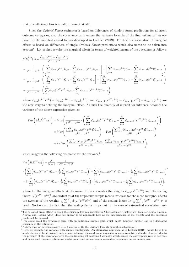
For the sake of brevity, here we focus mainly on the simulation results obtained for the simple and
for the complex DGP, while the results for all 72 DGPs are provided in Appendix B.2. Figures 1 and 2
summarize the results for the low-dimensional setting for the simple and the complex DGP, respectively.
Similarly, Figures 3 and 4 present the results for the simple and the complex DGP for the high-dimensional
setting. The upper panels of the figures show the ARPS, the preferred accuracy measure, whereas the
lower panels show the AMSE as a complementary measure. Within the figures the transparent boxplots in
the background show the results for the smaller sample size along with the bold boxplots in the foreground
showing the results for the bigger sample size. From left to right the figures present the results for 3, 6 and
9 outcome classes, respectively. The figures compare the prediction accuracy of the ordered logit, naive
forest, ordinal forest, conditional forest, Ordered Forest and the multinomial forest, where the asterisk (∗)
denotes the honest version of the last two forests considered. Further tables with more detailed results
and statistical tests for mean differences in the prediction errors are listed in Appendix B.1.
Figure 1: Simulation Results: Simple DGP & Low Dimension
Note: Figure summarizes the prediction accuracy results based on 100 simulation replications. The upper panel contains theARPS and the lower panel contains the AMSE. The boxplots show the median and the interquartile range of the respectivemeasure. The transparent boxplots denote the results for the small sample size, while the bold boxplots denote the resultsfor the big sample size. From left to right the results for 3, 6, and 9 outcome classes are displayed.
In the low-dimensional setting with the simple DGP it is expected that the ordered logistic regression
should perform best in terms of both the AMSE as well as the ARPS. Indeed, we do observe this results
in Figure 1 as the ordered logit model performs unanimously best out of the considered models, reaching
almost zero prediction error. Among the flexible forest-based estimators, the proposed Ordered Forest
belongs to those better performing methods in terms of both accuracy measures. The honest versions of
the forests lack behind what points at the efficiency loss due to the additional sample splitting. Overall,
14
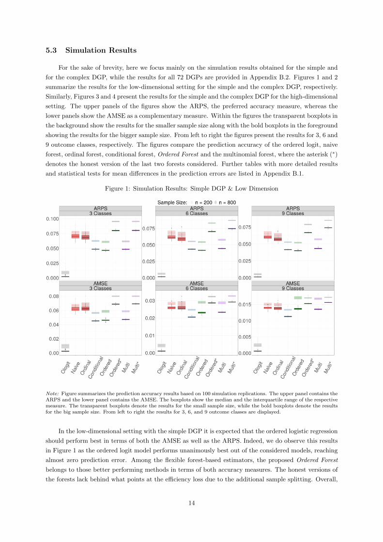
the ranking of the estimators stays stable with regards to the number of outcome categories. Additional
pattern common to all estimators is the lower prediction error and increased precision with growing
sample size.
Figure 2: Simulation Results: Complex DGP & Low Dimension
Note: Figure summarizes the prediction accuracy results based on 100 simulation replications. The upper panel contains theARPS and the lower panel contains the AMSE. The boxplots show the median and the interquartile range of the respectivemeasure. The transparent boxplots denote the results for the small sample size, while the bold boxplots denote the resultsfor the big sample size. From left to right the results for 3, 6, and 9 outcome classes are displayed.
In the case of the complex DGP, the performance of the flexible forest-based estimators is expected
to be better in comparison to the parametric ordered logit. This can be seen in Figure 2 as the ordered
logit lacks behind the majority of the flexible methods in both accuracy measures. The somewhat higher
prediction errors of the naive and the ordinal forest compared to the other forest-based methods might
be due to their different primary target which are the ordered classes instead of the ordered probabilities
as is the case for the other methods. In this respect the conditional forest exhibits considerably good
prediction performance. The Ordered Forest outperforms the competing forest-based estimators in terms
of the ARPS throughout all outcome class scenarios and also in terms of the AMSE in two scenarios, being
outperformed only by the conditional forest in case of 9 outcome classes. Interestingly, the multinomial
forest performs very well across all scenarios. However, it is consistently worse than the Ordered Forest
with bigger discrepancy between the two the more outcome classes are considered. This points to the
value of the ordering information and the ability of the Ordered Forest to utilize it in the estimation.
With regards to the sample size, we observe the same pattern as in Figure 1.
15
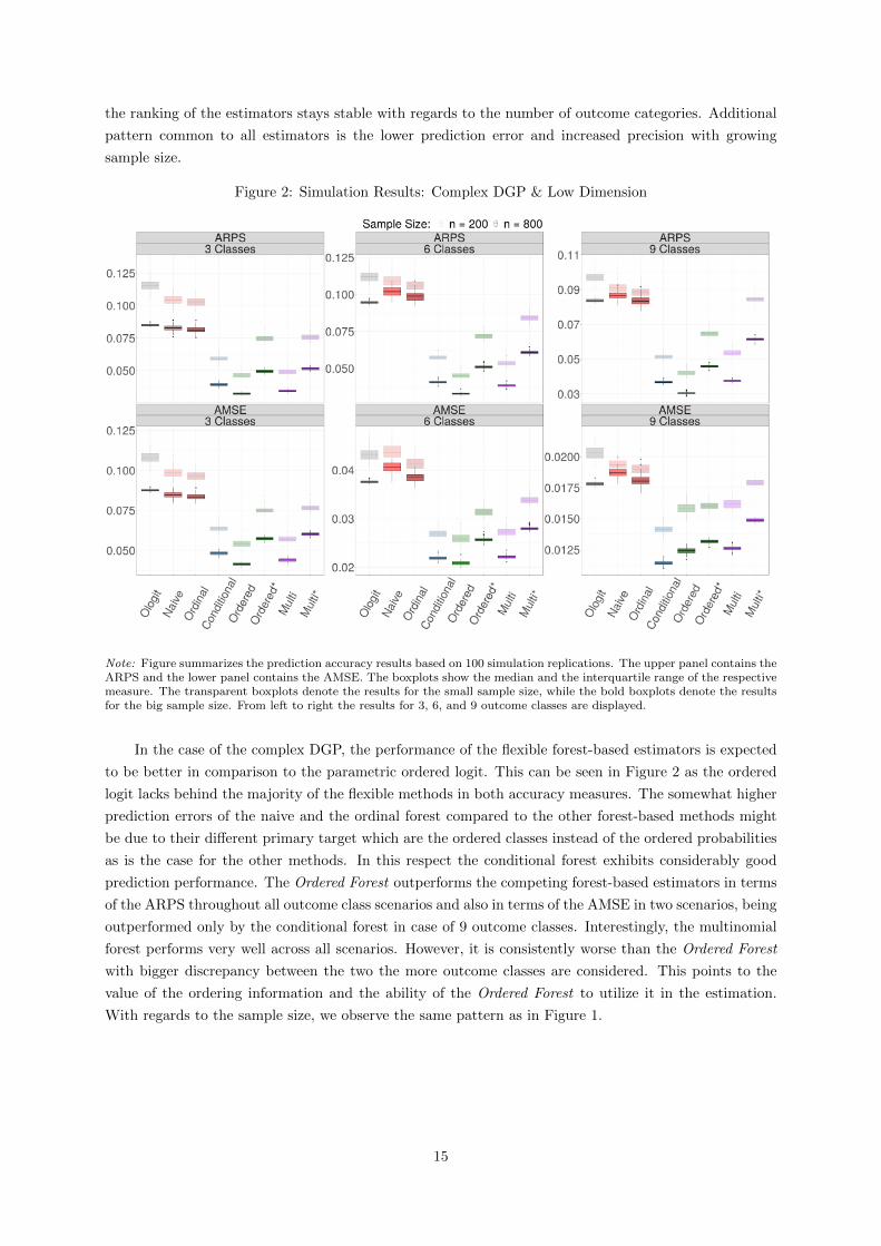
Figure 3: Simulation Results: Simple DGP & High Dimension
Note: Figure summarizes the prediction accuracy results based on 100 simulation replications. The upper panel contains theARPS and the lower panel contains the AMSE. The boxplots show the median and the interquartile range of the respectivemeasure. The transparent boxplots denote the results for the small sample size, while the bold boxplots denote the resultsfor the big sample size. From left to right the results for 3, 6, and 9 outcome classes are displayed.
Considering the high-dimensional setting for the case of the simple DGP, we see in Figure 3 that the
Ordered Forest slightly lacks behind the other methods, except the scenarios with 3 outcome classes. In
comparison, the conditional forest performs best in terms of the ARPS as well as in terms of the AMSE.
Also the naive and the ordinal forest exhibit better performance compared to the previous simulation
designs. However, it should be noted that the overall differences in the magnitude of the prediction errors
are much lower within this simulation design as compared to the previous designs. Further, taking a
closer look at the ARPS results of the multinomial forest we clearly see that in the simple ordered design
the ignorance of the ordering information really harms the predictive performance of the estimator the
more outcome classes are considered. Additionally, it is interesting to see that the performance gain due
to a bigger sample size seems to be much less for the honest version of the forests in the high-dimensional
setting as opposed to the low-dimensional setting.
16
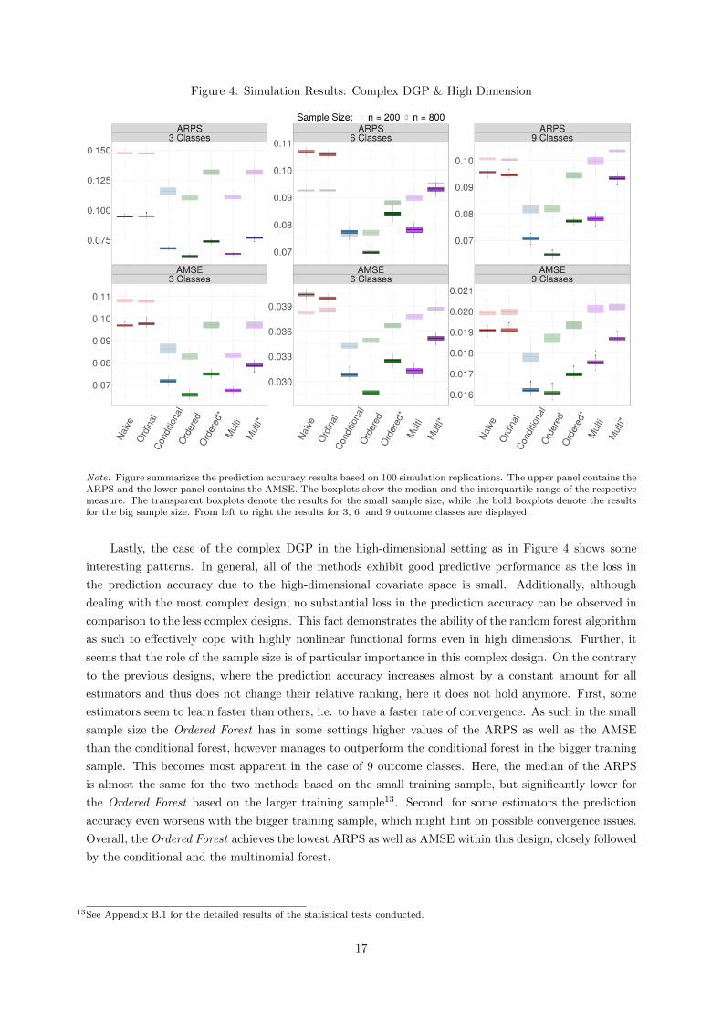
Figure 4: Simulation Results: Complex DGP & High Dimension
Note: Figure summarizes the prediction accuracy results based on 100 simulation replications. The upper panel contains theARPS and the lower panel contains the AMSE. The boxplots show the median and the interquartile range of the respectivemeasure. The transparent boxplots denote the results for the small sample size, while the bold boxplots denote the resultsfor the big sample size. From left to right the results for 3, 6, and 9 outcome classes are displayed.
Lastly, the case of the complex DGP in the high-dimensional setting as in Figure 4 shows some
interesting patterns. In general, all of the methods exhibit good predictive performance as the loss in
the prediction accuracy due to the high-dimensional covariate space is small. Additionally, although
dealing with the most complex design, no substantial loss in the prediction accuracy can be observed in
comparison to the less complex designs. This fact demonstrates the ability of the random forest algorithm
as such to effectively cope with highly nonlinear functional forms even in high dimensions. Further, it
seems that the role of the sample size is of particular importance in this complex design. On the contrary
to the previous designs, where the prediction accuracy increases almost by a constant amount for all
estimators and thus does not change their relative ranking, here it does not hold anymore. First, some
estimators seem to learn faster than others, i.e. to have a faster rate of convergence. As such in the small
sample size the Ordered Forest has in some settings higher values of the ARPS as well as the AMSE
than the conditional forest, however manages to outperform the conditional forest in the bigger training
sample. This becomes most apparent in the case of 9 outcome classes. Here, the median of the ARPS
is almost the same for the two methods based on the small training sample, but significantly lower for
the Ordered Forest based on the larger training sample13. Second, for some estimators the prediction
accuracy even worsens with the bigger training sample, which might hint on possible convergence issues.
Overall, the Ordered Forest achieves the lowest ARPS as well as AMSE within this design, closely followed
by the conditional and the multinomial forest.
13See Appendix B.1 for the detailed results of the statistical tests conducted.
17
In addition to the four main simulation designs discussed above, we also inspect all 72 different
DGPs (see Appendix B.2) to analyze the performance and the sensitivity of the respective estimators to
the particular features of the simulated DGPs. Let us first consider the low-dimensional case. Here, the
first observation we make is the robustness of the ordered logit to small deviations from the simple DGP.
As such, the prediction performance of the ordered logit does not worsen much if either noise variables,
randomly spaced thresholds, or a limited multicollinearity is introduced within the DGP at a time. How-
ever, the prediction performance further worsens if these features are introduced combined. Nevertheless,
the ordered logit predictions deteriorate substantially in all DGPs which include nonlinear effects, both
separately as well as combined with other features. On the contrary, all forest-based estimators do well
in these DGPs and clearly outperform the ordered logit. This points to the ability of random forests to
naturally deal with nonlinear functional forms. Among the forest-based estimators the Ordered Forest
outperforms the other methods particularly if the nonlinear effects are accompanied by multicollinearity
of regressors as such as well as together with additional noise variables or randomly spaced thresholds
(see DGPs 9, 12, 15 in Table 9, DGPs 25, 28, 31 in Table 10, and DGPs 41, 44, 47 in Table 11). Overall,
the Ordered Forest and the conditional forest turn out to be more robust to different DGPs in terms of
the prediction performance than the naive and the ordinal forest. The above results are homogeneous in
respect to the number of outcome classes which corresponds also to the finding in the simulation study
of Hornung (2019a). Thus, the number of outcome classes does not influence the relative performance of
the considered estimators.
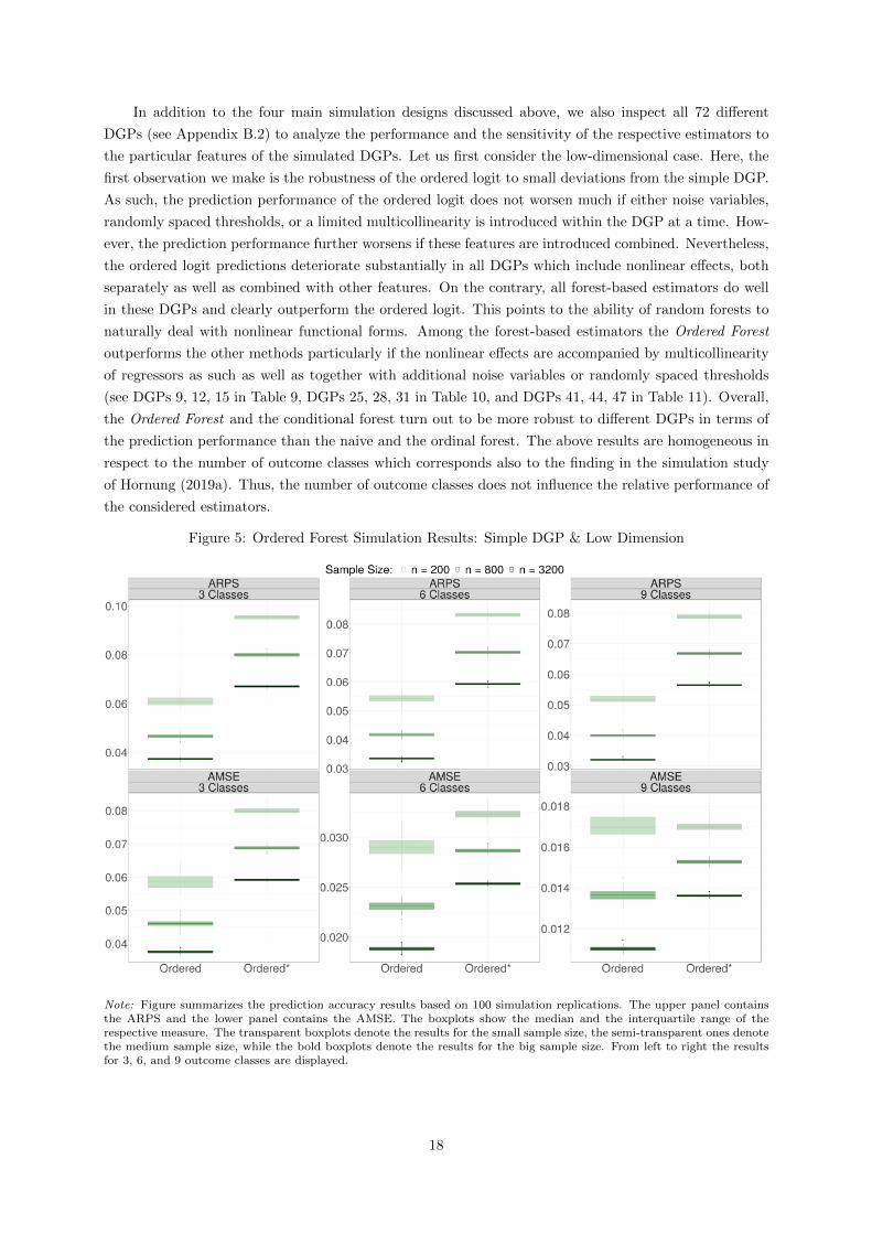
Figure 5: Ordered Forest Simulation Results: Simple DGP & Low Dimension
Note: Figure summarizes the prediction accuracy results based on 100 simulation replications. The upper panel containsthe ARPS and the lower panel contains the AMSE. The boxplots show the median and the interquartile range of therespective measure. The transparent boxplots denote the results for the small sample size, the semi-transparent ones denotethe medium sample size, while the bold boxplots denote the results for the big sample size. From left to right the resultsfor 3, 6, and 9 outcome classes are displayed.
18

Next, considering the high-dimensional case, we again observe a good prediction accuracy of the
forest-based methods when dealing with nonlinear effects as such. When these are combined with ran-
domly spaced thresholds the naive and the ordinal forest achieve better accuracy than the other methods.
However, if the randomly spaced thresholds are introduced without additional nonlinearities the condi-
tional forest outperforms the other methods. Further, the Ordered Forest exhibits again good performance
when dealing with multicollinearity and outperforms the other estimators in this respect as well as com-
bined with the randomly spaced thresholds (see DGPs 51, 55 in Table 12, DGPs 59, 63 in Table 13,
and DGPs 67, 71 in Table 14). For the case of multicollinearity combined with nonlinearities, both the
Ordered Forest and the conditional forest achieve good prediction accuracy and one cannot discriminate
between the two methods. Possibly, a bigger sample size would be needed in order to do so, as we have
seen in the case of the complex DGP above. Lastly, similarly to the low-dimensional case, we do not
observe any substantial differences in the relative prediction performance in respect to the number of
outcome classes. In general, both in the low-dimensional as well as in the high-dimensional case, the
honest version of the Ordered Forest achieves consistently lower prediction accuracy. It seems that in
small samples the increase in variance due to honesty prevails the reduction in bias of the estimator.
Figure 6: Ordered Forest Simulation Results: Complex DGP & Low Dimension
Note: Figure summarizes the prediction accuracy results based on 100 simulation replications. The upper panel containsthe ARPS and the lower panel contains the AMSE. The boxplots show the median and the interquartile range of therespective measure. The transparent boxplots denote the results for the small sample size, the semi-transparent ones denotethe medium sample size, while the bold boxplots denote the results for the big sample size. From left to right the resultsfor 3, 6, and 9 outcome classes are displayed.
In order to further investigate the impact of the honesty feature in bigger samples as well as the
convergence of the Ordered Forest, we quadruple the size of the training set once again and repeat the
main simulation for the Ordered Forest and its honest version with N = 3200 observations. As in the
main analysis Figures 5 and 6 show the simulation results for the simple and the complex DGP in the
low-dimensional case, while Figures 7 and 8 present the results of the two DGPs in the high-dimensional
19

setting. Within the tables the transparent boxplots denote the smallest sample size (N = 200), the
semi-transparent boxplots show the medium sample size (N = 800), while the bold boxplots indicate the
results for the biggest sample size (N = 3200). Similarly to the above, the upper panels of the figures
show the ARPS and the lower panels show the AMSE, whereas the results for 3, 6, and 9 outcome classes
are displayed fom left to right. More detailed results are included in Table 8 in Appendix B.1.
Figure 7: Ordered Forest Simulation Results: Simple DGP & High Dimension
Note: Figure summarizes the prediction accuracy results based on 100 simulation replications. The upper panel containsthe ARPS and the lower panel contains the AMSE. The boxplots show the median and the interquartile range of therespective measure. The transparent boxplots denote the results for the small sample size, the semi-transparent ones denotethe medium sample size, while the bold boxplots denote the results for the big sample size. From left to right the resultsfor 3, 6, and 9 outcome classes are displayed.
The first observation we make is the convergence of both versions of the estimator in all considered
scenarios (obviously based on three data points only). With growing sample size the prediction errors get
lower and the precision increases. However, the rate of convergence seems to be slower than the parametric√N rate. Clearly, this is the price to pay for the additional flexibility of the estimator. Interestingly,
the convergence in MSE appears to be slightly slower for the high-dimensional case in comparison to
the low-dimensional case, pointing to the theoretically limited scope of the curse of dimensionality of the
forests. Generally, we also see somewhat higher prediction errors in the high-dimensional compared to
the low-dimensional settings. With regards to the honesty feature, we observe the same pattern as in
the smaller sample sizes, namely slightly lower prediction accuracy for the honest version of the Ordered
Forest in all four simulation designs. The loss in the prediction accuracy due to honesty appears to be
roughly constant across the considered scenarios, while in some cases, such as the complex DGP in low
dimension (Figure 6), the difference in the prediction error gets smaller with bigger sample size. However,
in other cases, such as the simple DGP in high dimension (Figure 7), this difference gets larger. Hence,
even in the biggest sample the additional variance dominates the bias reduction. However, for a prediction
exercise honesty is an optional choice, while if inference is of interest, honesty becomes binding.
20

Figure 8: Ordered Forest Simulation Results: Complex DGP & High Dimension
Note: Figure summarizes the prediction accuracy results based on 100 simulation replications. The upper panel containsthe ARPS and the lower panel contains the AMSE. The boxplots show the median and the interquartile range of therespective measure. The transparent boxplots denote the results for the small sample size, the semi-transparent ones denotethe medium sample size, while the bold boxplots denote the results for the big sample size. From left to right the resultsfor 3, 6, and 9 outcome classes are displayed.
Finally, it should be noted that there is no ’one fits all’ estimator and the choice of the particular
method should be carefully done and guided by particular aspects of the estimation problem at hand.
Nevertheless, the conducted simulation study provides an evidence for a good predictive performance of
the new Ordered Forest estimator in the estimations of various ordered choice models.
6 Empirical Applications
In this section we explore the performance of the Ordered Forest estimator based on real datasets14
previously used in Janitza et al. (2016) and Hornung (2019a). First, we compare our estimator in terms
of the prediction accuracy to all the estimators used in the above Monte Carlo simulation. Second, we
compare the Ordered Forest estimator also in terms of estimating marginal effects to the parametric
ordered logit model. We do not consider the other forest based estimators here as these do not provide
marginal effects estimation. Table 2 summarizes the datasets and the descriptive statistics are provided
in Appendix C.1.
14The here proposed algorithm has been already applied and is in use for predicting match outcomes in football, see Golleret al. (2018) and SEW Soccer Analytics for details.
21

Table 2: Description of the Datasets
Datasets Summary
Dataset Sample Size Outcome Class Range Covariates
Wine Quality 4893 Quality Score 1 (moderate) - 6 (high) 11Mammography 412 Visits History 1 (never) - 3 (over year) 5Nhanes 1914 Health Status 1 (excellent) - 5 (poor) 26Vlbw 218 Physical Condition 1 (threatening) - 9 (optimal) 10Support Study 798 Disability Degree 1 (none) - 5 (fatal) 15
6.1 Prediction Accuracy
Similarly to Hornung (2019a) we evaluate the prediction accuracy based on a repeated cross-validation
in order to reduce the dependency of the results on the particular training and test sample splits. As such
we perform a 10-fold cross-validation on each dataset, i.e. we randomly split the dataset in 10 equally
sized folds and use 9 folds for training the model and 1 fold for validation. This process is repeated such
that each fold serves as a validation set exactly once. Lastly, we repeat this whole procedure 10 times
and report average accuracy measures. The results of the cross-validation exercise for the ARPS as well
as the AMSE are summarized in Figures 9 and 10, respectively. Similarly as for the simulation results
Appendix C.2 contains more detailed statistics.
Figure 9: Cross-Validation: ARPS
Note: Figure summarizes the prediction accuracy results in terms of the ARPS based on 10 repetitions of 10-fold cross-validation for respective datasets. The boxplots show the median and the interquartile range of the respective measure.
22

The main difference in evaluating the prediction accuracy in comparison to the simulation study
is the fact that we do not observe the outcome probabilities, but only the realized outcomes. This
affects the computation of the accuracy measures as mentioned in Section 5.2 and it can be expected
that the prediction errors are somewhat higher in comparison to the simulation data, which is also
the case here. Overall, the results imply a substantial heterogeneity in the prediction accuracy across
the considered datasets. On the one hand, the parametric ordered logit does well in small samples
(vlbw) whereas the forest-based methods are somewhat lacking behind. This is not surprising as a lower
precision in small samples is the price to pay for the additional flexibility. On the other hand, in the
largest sample (winequality) the ordered logit is clearly the worst performing method and all forest-based
methods perform substantially better. With respect to the Ordered Forest estimator we observe relatively
high prediction accuracy for three datasets (mammography, supportstudy, winequality) and relatively low
prediction accuracy for two datasets (nhanes, vlbw) in comparison to the competing methods. The good
performance in the winequality and the supportstudy dataset is expected due to the large samples available.
In case of the mammography dataset, even when smaller in sample size, the Ordered Forest maintains the
good prediction performance, with its honest version doing even better. The worse performance for the
vlbw dataset might be due to the small sample size. However, the honest version of the Ordered Forest
performs rather well. The relatively poor performance in the case of the nhanes dataset comes rather
at surprise as the sample size is large. Nevertheless, here the differences among all estimators are very
small in magnitude, in fact the smallest among the considered datasets.
Figure 10: Cross-Validation: AMSE
Note: Figure summarizes the prediction accuracy results in terms of the AMSE based on 10 repetitions of 10-fold cross-validation for respective datasets. The boxplots show the median and the interquartile range of the respective measure.
23

6.2 Marginal Effects
In order to analyze the relationship between the covariates and the predicted choice probabilities we
estimate the marginal effects for the Ordered Forest and compare these to the marginal effects estimated
by the ordered logit. We estimate both common measures for marginal effects, i.e. the mean marginal
effects as well as the marginal effects at covariate means. The main difference between the ordered logit
and the Ordered Forest is the fact that the Ordered Forest does not use any parametric link function in
the estimation of the marginal effects and as such does not impose any functional form on these estimates.
As a result, the Ordered Forest does neither fix the sign of the marginal effects estimates nor revert it
exactly once within the class range as is the case for the ordered logit (the so-called ’single crossing’
feature, see i.e. Boes and Winkelmann (2006) or Greene and Hensher (2010)) but rather estimates these
in a data-driven manner. Nevertheless, the Ordered Forest, same as the ordered logit, still ensures that
the marginal effects across the class range sum up to zero (being more likely to be in the highest class
must imply being less likely to be in the lowest class). As such the Ordered Forest not only enables a
more flexible estimation of the choice probabilities but also of the marginal effects. Table 3 compares the
mean marginal effects estimated by the Ordered Forest and the ordered logit for the winequality dataset,
whereas Appendix C.3 contains the mean marginal effects and the marginal effects at mean for all the
other datasets. The winequality dataset is particularly suitable for such comparison as it contains only
continuous covariates which are natural for evaluation of the marginal effects and has also a sufficiently
large sample size with well represented outcome classes. Table 3 contains the estimated effects for each
outcome class of each covariate together with the associated standard errors, t-values, p-values as well as
conventional significance levels for both the Ordered Forest as well as the ordered logit.
Table 3: Mean Marginal Effects: Wine Quality Dataset
Dataset Ordered Forest Ordered Logit
Variable Class Effect Std.Error t-Value p-Value Effect Std.Error t-Value p-Value
alcohol 1 0.0000 0.0001 0.4559 0.6484 -0.0017 0.0005 -3.5943 0.0003 ***
2 -0.0023 0.0021 -1.0701 0.2846 -0.0125 0.0023 -5.4096 0.0000 ***
3 -0.0582 0.0055 -10.5215 0.0000 *** -0.0612 0.0105 -5.8009 0.0000 ***
4 0.0189 0.0063 2.9994 0.0027 *** 0.0163 0.0031 5.2566 0.0000 ***
5 0.0341 0.0059 5.7334 0.0000 *** 0.0450 0.0077 5.8232 0.0000 ***
6 0.0075 0.0076 0.9865 0.3239 0.0141 0.0026 5.4111 0.0000 ***
chlorides 1 0.0011 0.0058 0.1924 0.8474 0.0023 0.0055 0.4147 0.6784
2 0.2323 0.0653 3.5565 0.0004 *** 0.0166 0.0398 0.4167 0.6769
3 1.1824 0.3295 3.5882 0.0003 *** 0.0811 0.1945 0.4169 0.6768
4 0.0187 0.5868 0.0319 0.9745 -0.0216 0.0518 -0.4175 0.6763
5 -1.3851 0.4807 -2.8816 0.0040 *** -0.0596 0.1431 -0.4166 0.6770
6 -0.0495 0.5009 -0.0988 0.9213 -0.0187 0.0449 -0.4166 0.6769
citric 1 0.0007 0.0003 2.7474 0.0060 *** -0.0004 0.0010 -0.4410 0.6592
acid 2 -0.0210 0.0077 -2.7142 0.0066 *** -0.0031 0.0070 -0.4429 0.6578
3 -0.0766 0.0376 -2.0340 0.0420 ** -0.0151 0.0340 -0.4429 0.6578
4 0.0541 0.0393 1.3771 0.1685 0.0040 0.0091 0.4420 0.6585
5 0.0444 0.0307 1.4465 0.1480 0.0111 0.0250 0.4432 0.6576
6 -0.0017 0.0186 -0.0936 0.9255 0.0035 0.0079 0.4428 0.6579
density 1 0.0182 0.0363 0.5027 0.6152 1.7954 0.4504 3.9861 0.0001 ***
2 0.8623 0.3202 2.6927 0.0071 *** 13.0220 1.9652 6.6264 0.0000 ***
3 9.7099 1.8904 5.1363 0.0000 *** 63.5943 8.4039 7.5672 0.0000 ***
4 -1.4862 2.7180 -0.5468 0.5845 -16.9605 2.5147 -6.7447 0.0000 ***
5 -7.8099 2.5273 -3.0902 0.0020 *** -46.7731 6.2827 -7.4447 0.0000 ***
6 -1.2944 2.4755 -0.5229 0.6010 -14.6781 2.1808 -6.7305 0.0000 ***
Continued on next page
24
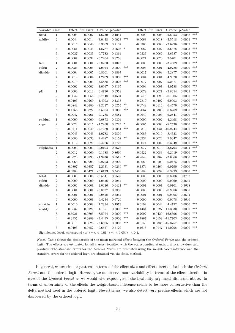
Variable Class Effect Std.Error t-Value p-Value Effect Std.Error t-Value p-Value
fixed 1 0.0003 0.0002 1.6239 0.1044 -0.0009 0.0003 -2.8953 0.0038 ***
acidity 2 0.0044 0.0014 3.0448 0.0023 *** -0.0063 0.0018 -3.5518 0.0004 ***
3 0.0015 0.0040 0.3669 0.7137 -0.0306 0.0083 -3.6996 0.0002 ***
4 -0.0081 0.0043 -1.8787 0.0603 * 0.0082 0.0022 3.6578 0.0003 ***
5 0.0027 0.0035 0.7782 0.4364 0.0225 0.0062 3.6587 0.0003 ***
6 -0.0007 0.0034 -0.2204 0.8256 0.0071 0.0020 3.5701 0.0004 ***
free 1 -0.0001 0.0001 -0.8283 0.4075 -0.0000 0.0000 -3.4689 0.0005 ***
sulfur 2 -0.0026 0.0005 -4.9064 0.0000 *** -0.0003 0.0001 -4.9288 0.0000 ***
dioxide 3 -0.0004 0.0005 -0.8601 0.3897 -0.0017 0.0003 -5.2877 0.0000 ***
4 0.0019 0.0004 4.2409 0.0000 *** 0.0004 0.0001 4.9370 0.0000 ***
5 0.0010 0.0003 3.5888 0.0003 *** 0.0012 0.0002 5.2571 0.0000 ***
6 0.0002 0.0002 1.0017 0.3165 0.0004 0.0001 4.9788 0.0000 ***
pH 1 0.0006 0.0012 0.4736 0.6358 -0.0079 0.0021 -3.8654 0.0001 ***
2 0.0042 0.0056 0.7548 0.4504 -0.0575 0.0093 -6.1905 0.0000 ***
3 -0.0403 0.0269 -1.4993 0.1338 -0.2810 0.0402 -6.9903 0.0000 ***
4 -0.0848 0.0380 -2.2337 0.0255 ** 0.0749 0.0116 6.4570 0.0000 ***
5 0.1156 0.0322 3.5904 0.0003 *** 0.2067 0.0303 6.8269 0.0000 ***
6 0.0047 0.0261 0.1785 0.8584 0.0649 0.0103 6.2841 0.0000 ***
residual 1 0.0000 0.0000 0.0873 0.9304 -0.0009 0.0002 -4.2498 0.0000 ***
sugar 2 -0.0028 0.0015 -1.7960 0.0725 * -0.0065 0.0008 -8.2530 0.0000 ***
3 -0.0111 0.0040 -2.7989 0.0051 *** -0.0319 0.0031 -10.2244 0.0000 ***
4 0.0046 0.0043 1.0783 0.2809 0.0085 0.0010 8.4523 0.0000 ***
5 0.0080 0.0033 2.4287 0.0152 ** 0.0234 0.0024 9.9347 0.0000 ***
6 0.0012 0.0029 0.4226 0.6726 0.0074 0.0009 8.3949 0.0000 ***
sulphates 1 -0.0003 0.0003 -0.9104 0.3626 -0.0072 0.0019 -3.8794 0.0001 ***
2 -0.0012 0.0069 -0.1688 0.8660 -0.0522 0.0083 -6.2919 0.0000 ***
3 -0.0570 0.0293 -1.9436 0.0519 * -0.2548 0.0362 -7.0366 0.0000 ***
4 0.0066 0.0293 0.2263 0.8209 0.0680 0.0109 6.2475 0.0000 ***
5 0.0807 0.0357 2.2631 0.0236 ** 0.1874 0.0269 6.9790 0.0000 ***
6 -0.0288 0.0471 -0.6123 0.5403 0.0588 0.0092 6.3993 0.0000 ***
total 1 -0.0000 0.0000 -0.5841 0.5592 0.0000 0.0000 0.8906 0.3732
sulfur 2 -0.0000 0.0000 -1.0456 0.2957 0.0000 0.0000 0.9069 0.3645
dioxide 3 0.0002 0.0001 2.0326 0.0421 ** 0.0001 0.0001 0.9101 0.3628
4 -0.0001 0.0001 -0.8627 0.3883 -0.0000 0.0000 -0.9086 0.3636
5 -0.0001 0.0001 -0.9828 0.3257 -0.0001 0.0001 -0.9095 0.3631
6 0.0000 0.0001 0.4234 0.6720 -0.0000 0.0000 -0.9078 0.3640
volatile 1 0.0010 0.0008 1.2894 0.1973 0.0198 0.0044 4.4792 0.0000 ***
acidity 2 0.0532 0.0129 4.1351 0.0000 *** 0.1434 0.0127 11.3030 0.0000 ***
3 0.6921 0.0805 8.5974 0.0000 *** 0.7002 0.0420 16.6696 0.0000 ***
4 -0.3955 0.0889 -4.4495 0.0000 *** -0.1867 0.0159 -11.7703 0.0000 ***
5 -0.3015 0.0826 -3.6505 0.0003 *** -0.5150 0.0335 -15.3757 0.0000 ***
6 -0.0493 0.0752 -0.6557 0.5120 -0.1616 0.0147 -11.0298 0.0000 ***
Significance levels correspond to: ∗ ∗ ∗. < 0.01, ∗ ∗ . < 0.05, ∗. < 0.1.
Notes: Table shows the comparison of the mean marginal effects between the Ordered Forest and the ordered
logit. The effects are estimated for all classes, together with the corresponding standard errors, t-values and
p-values. The standard errors for the Ordered Forest are estimated using the weight-based inference and the
standard errors for the ordered logit are obtained via the delta method.
In general, we see similar patterns in terms of the effect sizes and effect direction for both the Ordered
Forest and the ordered logit. However, we do observe more variability in terms of the effect direction in
case of the Ordered Forest as we would also expect given the flexibility argument discussed above. In
terms of uncertainty of the effects the weight-based inference seems to be more conservative than the
delta method used in the ordered logit. Nevertheless, we also detect very precise effects which are not
discovered by the ordered logit.
25

In particular, inspecting variables such as alcohol, volatile acidity, free sulfir dioxide or residual
sugar, both methods estimate comparable effects both in terms of the effect size as well as effect direction
with the difference of the Ordered Forest achieving a lower precision for the effects of the outer classes.
This might be in general due to lack of data for these outer classes (for class 1 only 20 data points are
available). Contrarily, in case of the variable density, even though the effect direction and the precision
are in line with the above, the ordered logit seems to overshoot the effect sizes quite substantially, most
probably due to the parametric extrapolation in comparison to the Ordered Forest which does not allow
any extrapolation by definition as the estimation of the effects respects the support of the covariates
and thus the Ordered Forest estimates the effects of an order of magnitude lower. Further, for variables
such as chlorides and citric acid the Ordered Forest identifies relevant effects which are not discovered
by the ordered logit. Particularly for chlorides, also the effect sizes are a bit larger and the turnaround
of the effect direction is shifted to a higher class. As such the effect stays positive for the first four
classes whereas the ordered logit forces the switch already after the third class. In addition, we observe
also variables such as total sulfur dioxide for which both of the methods find no evidence for relevant
effects, at most evidence for a zero effect. This might be due to collinearity issues with variable free sulfur
dioxide which takes up the whole effect of sulfur dioxide. Lastly, for some of the variables, namely fixed
acidity and pH the estimated effects differ substantially between the Ordered Forest and the ordered
logit. Overall, however, the main advantage of the estimation of the marginal effects by the Ordered
Forest stems from a more flexible, data-driven approximation of possible nonlinearities in the functional
form.
7 Conclusion
In this paper, we develop and apply a new machine learning estimator of the econometric ordered
choice models based on the random forest algorithm. The Ordered Forest estimator is a flexible alternative
to parametric ordered choice models such as the ordered logit or ordered probit which does not rely on any
distributional assumptions and provides essentially the same output as the parametric models, including
the estimation of the marginal effects as well as the associated inference. The proposed estimator utilizes
the flexibility of random forests and can thus naturally deal with nonlinearities in the data and with
a large-dimensional covariate space, while taking the ordering information of the categorical outcome
variable into account. Hence, the estimator flexibly estimates the conditional choice probabilities without
restrictive assumptions about the distribution of the error term, or other assumptions such as the single
index and constant threshold assumptions as is the case for the parametric ordered choice models (see
Boes and Winkelmann (2006) for a discussion of these assumptions). Further, the estimator allows also
the estimation of the marginal effects, i.e. how the estimated conditional choice probabilities vary with
changes in covariates. The weighted representation of these effects enables the weight-based inference as
suggested by Lechner (2019). The fact that the estimator comprises of linear combinations of random
forest predictions ensures the theoretical guarantees of Wager and Athey (2018). Additionally, a free
software implementation of the Ordered Forest estimator is available in GAUSS and also an R-package
will be submitted to the CRAN repository to enable the usage of the method by applied researchers.
The performance of the Ordered Forest estimator is studied and compared to other competing es-
timators in an extensive Monte Carlo simulation as well as using real datasets. The simulation results
suggest good performance of the estimator in finite samples, including also high-dimensional settings.
The advantages of the machine learning estimation compared to a parametric method become apparent
when dealing with multicollinearity and highly nonlinear functional forms. In such cases all of the con-
26
sidered forest-based estimators perform better than the ordered logit in terms of the prediction accuracy.
Among the forest-based estimators the Ordered Forest proposed in this paper performs well throughout
all simulated DGPs and outperforms the competing methods in the most complex simulation designs.
The empirical evidence using real datasets supports the findings from the Monte Carlo simulation. Ad-
ditionally, the estimation of the marginal effects as well as the inference procedure seems to work well in
the empirical examples.
Despite the attractive properties of the Ordered Forest estimator, many interesting questions are
left open. Particularly, a further extension of the Monte Carlo simulation to study the sensitivity of the
Ordered Forest in respect to tuning parameters of the underlying random forest as well as in respect to
different simulation designs would be of interest. Similarly, the performance of the estimator with and
without honesty for larger sample sizes should be further investigated. Also, the optimal choice of the size
of the window for evaluating the marginal effects would be worth to explore. Additionally, a theoretical
framework for the used weight-based inference would be valuable, in particular the specific conditions
needed for the weights to yield a consistent estimator of standard errors. Lastly, it would be of great
interest to see more real data applications of the Ordered Forest estimator, especially for large samples.
27

References
Agresti, Alan. Categorical Data Analysis. Vol. 45. 1. 2002, xv, 710 p. ST –Categorical data analysis.
Archer, Kellie J., Jiayi Hou, Qing Zhou, Kyle Ferber, John G. Layne, and Amanda E. Gentry. “Ordinal-
gmifs: An R package for ordinal regression in high-dimensional data settings”. In: Cancer Informatics
13 (2014), pp. 187–195.
Athey, Susan and Guido W. Imbens. “Recursive Partitioning for Heterogeneous Casaul Effects”. In:
Proceedings of the National Academy of Sciences 113.27 (2016), pp. 1–43.
Athey, Susan, Julie Tibshirani, and Stefan Wager. “Generalized random forests”. In: Annals of Statistics
47.2 (2019), pp. 1179–1203.
Biau, Gerard. “Analysis of a Random Forests Model”. In: Journal of Machine Learning Research 13
(2012), pp. 1063–1095.
Boes, Stefan and Rainer Winkelmann. “Ordered response models”. In: Modern Econometric Analysis:
Surveys on Recent Developments. 2006, pp. 167–181.
Breiman, L. “Random Forests”. In: Machine Learning 45.1 (2001), pp. 5–32.
Breiman, Leo. Classification and regression trees. 1984.
Brier, Glenn W. “Verification of Forecasts Expressed in Terms of Probability”. In: Monthly Weather
Review 78.1 (1950), pp. 1–3.
Cameron, A. Colin and Pavin K. Trivedi. Microeconometrics: methods and applications. Cambridge uni-
versity press. 2005.
Carsey, Thomas M. and Jeffrey J. Harden. Monte Carlo simulation and resampling methods for social
science. Sage Publications, 2013, pp. 1–294.
Chernozhukov, Victor, Denis Chetverikov, Mert Demirer, Esther Duflo, Christian Hansen, Whitney
Newey, and James Robins. “Double/debiased machine learning for treatment and structural param-
eters”. In: Econometrics Journal 21.1 (2018), pp. C1–C68.
Constantinou, Anthony Costa and Norman Elliott Fenton. “Solving the problem of inadequate scoring
rules for assessing probabilistic football forecast models”. In: Journal of Quantitative Analysis in
Sports 8.1 (2012).
Epstein, Edward S. “A Scoring System for Probability Forecasts of Ranked Categories”. In: Journal of
Applied Meteorology 8.6 (1969), pp. 985–987.
Fox, Jeremy T. “Semiparametric estimation of multinomial discrete-choice models using a subset of
choices”. In: RAND Journal of Economics 38.4 (2007), pp. 1002–1019.
Goller, Daniel, Michael C. Knaus, Michael Lechner, and Gabriel Okasa. “Predicting Match Outcomes in
Football by an Ordered Forest Estimator”. In: Economics Working Paper Series No.1811 (2018).
Greene, William H. and David A. Hensher. Modeling ordered choices: A primer. 2010, pp. 1–365.
Harrell, Frank E. “Regression modeling strategies: with applications to linear models, logistic and ordinal
regression, and survival analysis”. In: Springer (2015), p. 533.
— rms: Regression Modeling Strategies. 2019.
Hastie, Trevor, Robert Tibshirani, and Jerome Friedman. “The Elements of Statistical Learning”. In:
Elements 1 (2009).
Hornung, Roman. “Ordinal Forests”. In: Journal of Classification (2019).
— ordinalForest: Ordinal Forests: Prediction and Variable Ranking with Ordinal Target Variables. 2019.
Hothorn, Torsten, Peter Buhlmann, Sandrine Dudoit, Annette Molinaro, and Mark J. Van Der Laan.
“Survival ensembles”. In: Biostatistics 7.3 (2006), pp. 355–373.
28
Hothorn, Torsten, Kurt Hornik, and Achim Zeileis. “Unbiased recursive partitioning: A conditional in-
ference framework”. In: Journal of Computational and Graphical Statistics 15.3 (2006), pp. 651–674.
Hothorn, Torsten, Berthold Lausen, Axel Benner, and Martin Radespiel-Troger. “Bagging survival trees”.
In: Statistics in Medicine 23.1 (2004), pp. 77–91.
Ichimura, Hidehiko. “Semiparametric least squares (SLS) and weighted SLS estimation of single-index
models”. In: Journal of Econometrics 58.1-2 (1993), pp. 71–120.
Imbens, Guido W and Alberto Abadie. “Large Sample Properties of Matching Estimators for Average
Treatment Effects”. In: Econometrica 74.1 (2006), pp. 235–267.
Janitza, Silke, Gerhard Tutz, and Anne Laure Boulesteix. “Random forest for ordinal responses: Pre-
diction and variable selection”. In: Computational Statistics and Data Analysis 96 (2016), pp. 57–
73.
Klein, Roger W. and Robert P. Sherman. “Shift restrictions and semiparametric estimation in ordered
response models”. In: Econometrica 70.2 (2002), pp. 663–691.
Klein, Roger W. and Richard H. Spady. “An Efficient Semiparametric Estimator for Binary Response
Models”. In: Econometrica 61.2 (1993), p. 387.
Kramer, Stefan. “Structural Regression Trees”. In: AAAI-96 Proceedings (1996), pp. 812–819.
Kramer, Stefan, Gerhard Widmer, Bernhard Pfahringer, and Michael De Groeve. “Prediction of Ordinal
Classes Using Regression Trees *”. In: Fundamenta Informaticae 34 (2000), pp. 1–15.
Lechner, Michael. “Modified Causal Forests for Estimating Heterogeneous Causal Effects”. In: CEPR
Discussion Paper No. DP13430 (2019).
— Program heterogeneity and propensity score matching: An application to the evaluation of active labor
market policies. 2002.
Lee, Lung fei. “Semiparametric maximum likelihood estimation of polychotomous and sequential choice
models”. In: Journal of Econometrics 65.2 (1995), pp. 381–428.
Lewbel, Arthur. “Semiparametric qualitative response model estimation with unknown heteroscedasticity
or instrumental variables”. In: Journal of Econometrics 97.1 (2000), pp. 145–177.
Lin, Zhongjian, Qi Li, and Yiguo Sun. “A consistent nonparametric test of parametric regression func-
tional form in fixed effects panel data models”. In: Journal of Econometrics 178.PART 1 (2014),
pp. 167–179.
Loh, Wei-Yin. “Classification and regression trees”. In: WIREs Data Mining Knowl Discov 1 (2011),
pp. 14–23.
Matzkin, Rosa L. “Nonparametric and Distribution-Free Estimation of the Binary Threshold Crossing
and The Binary Choice Models”. In: Econometrica 60.2 (1992), pp. 239–270.
McCullagh, P and J A Nelder. Generalized Linear Models, Second Edition. 1989, p. 500.
McCullagh, Peter. “Regression Models for Ordinal Data”. In: Journal of the Royal Statistical Society.
Series B. 42.2 (1980), pp. 109–142.
Meinshausen, Nicolai. “Quantile Regression Forests”. In: Journal of Machine Learning Research 7 (2006),
pp. 983–999.
Mentch, Lucas and Giles Hooker. “Quantifying Uncertainty in Random Forests via Confidence Intervals
and Hypothesis Tests”. In: Journal of Machine Learning Research 17.1 (2016), pp. 1–41.
Piccarreta, Raffaella. “Classification trees for ordinal variables”. In: Computational Statistics 23.3 (2008),
pp. 407–427.
Powell, James L. and Thomas M. Stoker. “Optimal bandwidth choice for density-weighted averages”. In:
Journal of Econometrics 75.2 (1996), pp. 291–316.
R Core Team. R: A Language and Environment for Statistical Computing. Vienna, Austria, 2018.
29

Racine, Jeffrey S. “Nonparametric Econometrics: A Primer”. In: Foundations and Trends R© in Econo-
metrics 3.1 (2008), pp. 1–88.
Scornet, Erwan, Gerard Biau, and Jean Philippe Vert. “Consistency of random forests”. In: Annals of
Statistics 43.4 (2015), pp. 1716–1741.
Stewart, Mark B. “A comparison of semiparametric estimators for the ordered response model”. In:
Computational Statistics and Data Analysis 49.2 (2005), pp. 555–573.
Stoker, Thomas M. “Smoothing bias in the measurement of marginal effects”. In: Journal of Econometrics
72.1-2 (1996), pp. 49–84.
Strasser, Helmut and Christian Weber. “On the asymptotic theory of permutation statistics”. In: Math-
ematical Methods of Statistics 8 (1999), pp. 220–250.
Strobl, Carolin, Anne-Laure Boulesteix, Thomas Kneib, Thomas Augustin, and Achim Zeileis. “Condi-
tional variable importance for random forests.” In: BMC bioinformatics 9 (2008), p. 307.
Strobl, Carolin, Anne-Laure Boulesteix, Achim Zeileis, and Torsten Hothorn. “Bias in random forest
variable importance measures: illustrations, sources and a solution.” In: BMC bioinformatics 8 (2007),
p. 25.
Tibshirani, Julie, Susan Athey, Stefan Wager, Rina Friedberg, Luke Miner, and Marvin Wright. grf:
Generalized Random Forests (Beta). 2018.
Wager, Stefan. “Asymptotic theory for random forests”. In: arXiv preprint arXiv:1405.0352 (2014).
Wager, Stefan and Susan Athey. “Estimation and Inference of Heterogeneous Treatment Effects using
Random Forests”. In: Journal of the American Statistical Association (2018), pp. 1228–1242.
Williams, Richard. “Understanding and interpreting generalized ordered logit models”. In: Journal of
Mathematical Sociology 40.1 (2016), pp. 7–20.
Wooldridge, Jeffrey M. Econometric Analysis of Cross Section and Panel Data. 2010.
Wright, Marvin N. and Andreas Ziegler. “ranger : A Fast Implementation of Random Forests for High
Dimensional Data in C++ and R”. In: Journal of Statistical Software 77.1 (2017), pp. 1–17.
Wurm, Michael J., Paul J. Rathouz, and Bret M. Hanlon. “Regularized Ordinal Regression and the
ordinalNet R Package”. In: arXiv preprint arXiv:1706.05003 (2017), pp. 1–42.
30

A Other Machine Learning Estimators
A.1 Multinomial Forest
Considering the Ordered Forest estimator a possible modification for models with categorical outcome
variable without an inherent ordering appears to be straightforward. Instead of estimating cumulative
probabilities and afterwards isolating the respective class probabilities, we can estimate the class proba-
bilities Pm,i = P [Yi = m | Xi = x] directly. As such the binary outcomes are now constructed to indicate
the particular outcome classes separately. Then the random forest predictions for each class yield the con-
ditional choice probabilities which need to be afterwards normalized to sum up to 1. Formally, consider
(un)ordered categorical outcome variable Yi ∈ {1, ...,M} with classes m and sample size N(i = 1, ..., N).
Then, the estimation procedure can be described as follows:
1. Create M binary indicator variables such as
Ym,i = 1(Yi = m) for m = 1, ...,M. (A.1)
2. Estimate regression random forest for each of the M indicators.
3. Obtain predictions Ym,i = P [Ym,i = 1 | Xi = x] =∑N
i=1 wm,i(x)Ym,i.
4. Compute probabilities for each class
Pm,i = Ym,i for m = 1, ...,M (A.2)
Pm,i =Pm,i∑M
m=1 Pm,i
for m = 1, ...,M, (A.3)
where the equation (A.2) defines the probabilities of all M classes and subsequent equation (A.3) ensures
that the probabilities sum up to 1 as this might not be the case otherwise. Similarly to the Ordered
Forest estimator, also the multinomial forest is a linear combination of the respective forest predictions
and as such also inherits the theoretical properties stemming from random forest estimation as described
in Section 3.
A.2 Conditional Forest
The conditional forest as discussed in Section 2 is grown with the so-called conditional inference
trees. The main idea is to provide an unbiased way of recursive splitting of the trees using a test statistic
based on permutation tests (Strasser and Weber, 1999). To describe the estimation procedure, consider
an ordered categorical outcome Yi ∈ (1, ...,M) with ordered classes m and an sample size N(i = 1, ..., N).
Further, define binary case weights wi ∈ {0, 1} which determine if the observation is part of the current
leaf. Then, the algorithm developed by Hothorn et al. (2006b) can be described as follows:
1. Test the global null hypothesis of independence between any of the P covariates and the outcome,
for the particular case weights, given a bootstrap sample Zb. Afterwards, select the p-th covariate
Xi,p with the strongest association with the outcome Yi, or stop if the null hypothesis cannot be
31

rejected. The association is measured by a linear statistic T given as:
Tp(Zb, w) =
N∑i=1
wigp(Xi,p)h(Yi), (A.4)
where gp(·) and h(·) are specific transformation functions.
2. Split the covariate sample space Xp into two disjoint sets I and J with adapted case weights
wi1(Xi,p ∈ I) and wi1(Xi,p ∈ J ) determining the observations falling into the subset I and J ,
respectively. Then, the split is chosen by evaluating a two-sample statistic as a special case of A.4:
T Ip (Zb, w) =
N∑i=1
wi1(Xi,p ∈ I)h(Yi) (A.5)
for all possible subsets I of the covariate sample space Xp.
3. Repeat steps 1 and 2 recursively with modified case weights.
Hence, the above algorithm distinguishes between variable selection (step 1) and splitting rule (step 2),
while both relying on the variations of the test statistic Tp(Zb, w). In practice, however, the distribution
of this statistic under the null hypothesis is unknown and depends on the joint distribution of Yi and
Xi,p. For this reason, the permutation tests are applied to abstract from the dependency by fixing the
covariates and conditioning on all possible permutations of the outcomes. Then, the conditional mean
and covariance of the test statistic can be derived and the asymptotic distribution can be approximated
by Monte Carlo procedures, while Strasser and Weber (1999) proved its normality. Finally, variables and
splits are chosen according to the lowest p-value of the test statistic Tp(Zb, w) and T Ip (Zb, w), respectively.
Besides the permutation tests, the choice of the tranformation functions gp(·) and h(·) is important
and depends on the type of the variables. For continuous outcome and covariates, identity transformation
is suggested. For the case of an ordinal regression which is of interest here, the transformation function
is given through the score function s(m). If the underlying latent Y ∗i is unobserved, it is suggested
that s(m) = m and thus h(Yi) = Yi. Hence, in the tree building the ordered outcome is treated as a
continuous one (Janitza et al., 2016). Then, however, the leaf predictions are the choice probabilities
computed as proportions of the outcome classes falling within the leaf, instead of fitting a within leaf
constant. The final conditional forest predictions for the choice probabilities are the averaged conditional
tree probability predictions. Such obtained choice probabilities are analyzed in the Monte Carlo study
in Section 5.
A.3 Ordinal Forest
In the following, the algorithm for the ordinal forest as developed by Hornung (2019a) is described.
To begin with, consider an ordered categorical outcome Yi ∈ (1, ...,M) with ordered classes m and sample
size N(i = 1, ..., N). Then, for a set of optimization forests b = 1, ..., Bsets:
1. Draw M−1 uniformly distributed variables Db,m ∼ U(0, 1) and sort them according to their values.
Further, set Db,1 = 0 and Db,M+1 = 1.
2. Define a score set Sb,m = {Sb,1, ..., Sb,M} with scores constructed as Sb,m = Φ−1(Db,m+Db,m+1
2
)for
m = 1, ...,M , where Φ(·) is the cdf of the standard normal.
32
3. Create a new continuous outcome Zb,i = (Zb,1, ..., Zb,N ) by replacing each class value m of the
original ordered categorical Yi by the m-th value of the score set Sb,m for all m = 1, ...,M .
4. Use Zb,i as dependent variable and estimate a regression forest RFSb,mwith Bprior trees.
5. Obtain the out-of-bag (OOB) predictions for the continuous Zb,i and transform them into predic-
tions for Yi as follows: Yb,i = m if Zb,i ∈]Φ−1(Db,m,Φ
−1(Db,m+1)]
for all i = 1, ..., N .
6. Compute a performance measure for the given forest RFSb,mbased on some performance function
of type f(Yi, Yb,i).
After estimating Bsets of optimization forests, take Sbest of these which achieved the best performance
according to the performance function. Then, construct the final set of uniformly distributed variables
D1, ..., DM+1 as an average of those from Sbest for m = 1, ...,M +1. Finally, form the optimized score set
Sm = {S1, ..., SM} with scores constructed as Sm = Φ−1(Dm+Dm+1
2
)for m = 1, ...,M . The continuous
outcome Zi = (Z1, ..., ZN ) is then similarly as in the optimization procedure constructed by replacing each
m value of the original outcome Yi by the m-th value of the optimized score set Sm for all m = 1, ...,M .
Finally, estimate the regression forest RFfinal using Zi as the dependent variable. On one hand, the class
prediction of such an ordinal forest is one of the M ordered classes which has been predicted the most by
the respective trees of the forest. On the other hand, the probability prediction is obtained as a relative
frequency of trees predicting the particular class. Such predicted choice probabilities are analyzed in the
conducted Monte Carlo study in Section 5. Further, the so-called naive forest corresponds to the ordinal
forest with omitting the above described optimization procedure.
B Simulation Study
B.1 Main Simulation Results
In the following Tables 4, 5, 6, 7 and 8 are summarized the simulation results presented in Section
5.3 in the main text. Each table specifies the particular simulation design as follows: the column Class
indicates the number of outcome classes, Dim. specifies the dimension, DGP characterizes the data
generating process as defined in the main text and Statistic contains summary statistics of the simu-
lation results. In particular, the mean of the respective accuracy measure and its standard deviation.
Furthermore, rows t-test and wilcox-test contain the p-values of the parametric t-test as well as the non-
parametric Wilcoxon test for the equality of means between the results of the Ordered Forest and all the
other methods. The alternative hypothesis is that the mean of the Ordered Forest is less than the mean
of the other method to test if the Ordered Forest achieves significantly lower prediction error than the
other considered methods.
33

B.1.1 ARPS: Sample Size = 200
Table 4: Simulation results: Accuracy Measure = ARPS & Sample Size = 200
Simulation Design Comparison of Methods
Class Dim. DGP Statistic Ologit Naive Ordinal Cond. Ordered Ordered* Multi Multi*
3 Low Simple mean 0.0097 0.0765 0.0755 0.0625 0.0609 0.0954 0.0619 0.0954st.dev. 0.0042 0.0056 0.0055 0.0018 0.0020 0.0011 0.0019 0.0012t-test 1.0000 0.0000 0.0000 0.0000 0.0000 0.0002 0.0000wilcox-test 1.0000 0.0000 0.0000 0.0000 0.0000 0.0000 0.0000
3 Low Complex mean 0.1156 0.1044 0.1028 0.0593 0.0466 0.0748 0.0491 0.0760st.dev. 0.0047 0.0039 0.0038 0.0023 0.0026 0.0028 0.0024 0.0027t-test 0.0000 0.0000 0.0000 0.0000 0.0000 0.0000 0.0000wilcox-test 0.0000 0.0000 0.0000 0.0000 0.0000 0.0000 0.0000
3 High Simple mean 0.1135 0.1139 0.1112 0.1140 0.1180 0.1139 0.1179st.dev. 0.0009 0.0010 0.0009 0.0008 0.0006 0.0008 0.0006t-test 1.0000 0.7676 1.0000 0.0000 0.7268 0.0000wilcox-test 0.9999 0.8438 1.0000 0.0000 0.7191 0.0000
3 High Complex mean 0.1476 0.1474 0.1156 0.1102 0.1316 0.1110 0.1317st.dev. 0.0013 0.0010 0.0041 0.0029 0.0031 0.0029 0.0031t-test 0.0000 0.0000 0.0000 0.0000 0.0287 0.0000wilcox-test 0.0000 0.0000 0.0000 0.0000 0.0272 0.0000
6 Low Simple mean 0.0062 0.0687 0.0665 0.0554 0.0544 0.0833 0.0577 0.0872st.dev. 0.0020 0.0048 0.0050 0.0012 0.0014 0.0009 0.0016 0.0010t-test 1.0000 0.0000 0.0000 0.0000 0.0000 0.0000 0.0000wilcox-test 1.0000 0.0000 0.0000 0.0000 0.0000 0.0000 0.0000
6 Low Complex mean 0.1122 0.1093 0.1058 0.0574 0.0452 0.0719 0.0536 0.0842st.dev. 0.0040 0.0045 0.0044 0.0017 0.0020 0.0022 0.0021 0.0024t-test 0.0000 0.0000 0.0000 0.0000 0.0000 0.0000 0.0000wilcox-test 0.0000 0.0000 0.0000 0.0000 0.0000 0.0000 0.0000
6 High Simple mean 0.0974 0.0972 0.0951 0.0983 0.1012 0.0998 0.1016st.dev. 0.0006 0.0006 0.0006 0.0005 0.0004 0.0005 0.0004t-test 1.0000 1.0000 1.0000 0.0000 0.0000 0.0000wilcox-test 1.0000 1.0000 1.0000 0.0000 0.0000 0.0000
6 High Complex mean 0.0927 0.0927 0.0766 0.0772 0.0882 0.0898 0.0952st.dev. 0.0006 0.0005 0.0020 0.0016 0.0014 0.0018 0.0006t-test 0.0000 0.0000 0.9878 0.0000 0.0000 0.0000wilcox-test 0.0000 0.0000 0.9887 0.0000 0.0000 0.0000
9 Low Simple mean 0.0054 0.0653 0.0629 0.0528 0.0519 0.0789 0.0569 0.0850st.dev. 0.0018 0.0042 0.0042 0.0012 0.0014 0.0009 0.0017 0.0009t-test 1.0000 0.0000 0.0000 0.0000 0.0000 0.0000 0.0000wilcox-test 1.0000 0.0000 0.0000 0.0000 0.0000 0.0000 0.0000
9 Low Complex mean 0.0973 0.0912 0.0887 0.0515 0.0421 0.0647 0.0537 0.0845st.dev. 0.0031 0.0033 0.0032 0.0015 0.0016 0.0019 0.0018 0.0017t-test 0.0000 0.0000 0.0000 0.0000 0.0000 0.0000 0.0000wilcox-test 0.0000 0.0000 0.0000 0.0000 0.0000 0.0000 0.0000
9 High Simple mean 0.0921 0.0918 0.0900 0.0931 0.0959 0.0955 0.0964st.dev. 0.0006 0.0006 0.0006 0.0005 0.0003 0.0004 0.0003t-test 1.0000 1.0000 1.0000 0.0000 0.0000 0.0000wilcox-test 1.0000 1.0000 1.0000 0.0000 0.0000 0.0000
9 High Complex mean 0.1007 0.1004 0.0817 0.0819 0.0945 0.0997 0.1036st.dev. 0.0007 0.0007 0.0020 0.0017 0.0015 0.0019 0.0006t-test 0.0000 0.0000 0.7875 0.0000 0.0000 0.0000wilcox-test 0.0000 0.0000 0.8473 0.0000 0.0000 0.0000
Notes: Table reports the average measures of the RPS based on 100 simulation replications for the sample size of 200observations. The first column denotes the number of outcome classes. Columns 2 and 3 specify the dimension and the DGP,respectively. The fourth column Statistic shows the mean and the standard deviation of the accuracy measure for all methods.Additionally, t-test and wilcox-test contain the p-values of the parametric t-test as well as the nonparametric Wilcoxon testfor the equality of means between the results of the Ordered Forest and all the other methods.
34

B.1.2 AMSE: Sample Size = 200
Table 5: Simulation results: Accuracy Measure = AMSE & Sample Size = 200
Simulation Design Comparison of Methods
Class Dim. DGP Statistic Ologit Naive Ordinal Cond. Ordered Ordered* Multi Multi*
3 Low Simple mean 0.0103 0.0669 0.0682 0.0565 0.0587 0.0800 0.0587 0.0800st.dev. 0.0044 0.0041 0.0044 0.0015 0.0022 0.0009 0.0016 0.0010t-test 1.0000 0.0000 0.0000 1.0000 0.0000 0.3900 0.0000wilcox-test 1.0000 0.0000 0.0000 1.0000 0.0000 0.2614 0.0000
3 Low Complex mean 0.1081 0.0985 0.0965 0.0637 0.0543 0.0752 0.0572 0.0768st.dev. 0.0039 0.0034 0.0029 0.0020 0.0026 0.0021 0.0022 0.0019t-test 0.0000 0.0000 0.0000 0.0000 0.0000 0.0000 0.0000wilcox-test 0.0000 0.0000 0.0000 0.0000 0.0000 0.0000 0.0000
3 High Simple mean 0.0923 0.0931 0.0908 0.0930 0.0952 0.0926 0.0952st.dev. 0.0008 0.0013 0.0009 0.0009 0.0007 0.0007 0.0007t-test 1.0000 0.2408 1.0000 0.0000 0.9980 0.0000wilcox-test 1.0000 0.5433 1.0000 0.0000 0.9977 0.0000
3 High Complex mean 0.1081 0.1079 0.0863 0.0828 0.0970 0.0834 0.0971st.dev. 0.0012 0.0009 0.0028 0.0019 0.0021 0.0020 0.0021t-test 0.0000 0.0000 0.0000 0.0000 0.0264 0.0000wilcox-test 0.0000 0.0000 0.0000 0.0000 0.0364 0.0000
6 Low Simple mean 0.0043 0.0284 0.0283 0.0248 0.0291 0.0324 0.0287 0.0327st.dev. 0.0014 0.0012 0.0018 0.0007 0.0010 0.0005 0.0008 0.0005t-test 1.0000 1.0000 0.9998 1.0000 0.0000 0.9958 0.0000wilcox-test 1.0000 1.0000 1.0000 1.0000 0.0000 0.9953 0.0000
6 Low Complex mean 0.0433 0.0438 0.0413 0.0270 0.0260 0.0314 0.0274 0.0339st.dev. 0.0014 0.0017 0.0014 0.0008 0.0011 0.0009 0.0010 0.0008t-test 0.0000 0.0000 0.0000 0.0000 0.0000 0.0000 0.0000wilcox-test 0.0000 0.0000 0.0000 0.0000 0.0000 0.0000 0.0000
6 High Simple mean 0.0352 0.0352 0.0347 0.0361 0.0361 0.0360 0.0361st.dev. 0.0003 0.0004 0.0004 0.0004 0.0004 0.0003 0.0004t-test 1.0000 1.0000 1.0000 0.8112 0.9994 0.6394wilcox-test 1.0000 1.0000 1.0000 0.8788 0.9989 0.6579
6 High Complex mean 0.0383 0.0386 0.0343 0.0350 0.0367 0.0378 0.0387st.dev. 0.0003 0.0004 0.0006 0.0005 0.0005 0.0005 0.0004t-test 0.0000 0.0000 1.0000 0.0000 0.0000 0.0000wilcox-test 0.0000 0.0000 1.0000 0.0000 0.0000 0.0000
9 Low Simple mean 0.0025 0.0150 0.0149 0.0134 0.0170 0.0170 0.0168 0.0172st.dev. 0.0008 0.0005 0.0007 0.0004 0.0006 0.0003 0.0005 0.0002t-test 1.0000 1.0000 1.0000 1.0000 0.5492 0.9993 0.0040wilcox-test 1.0000 1.0000 1.0000 1.0000 0.3269 0.9985 0.0003
9 Low Complex mean 0.0203 0.0194 0.0190 0.0142 0.0159 0.0161 0.0162 0.0179st.dev. 0.0006 0.0006 0.0005 0.0003 0.0005 0.0003 0.0004 0.0003t-test 0.0000 0.0000 0.0000 1.0000 0.0006 0.0000 0.0000wilcox-test 0.0000 0.0000 0.0000 1.0000 0.0004 0.0000 0.0000
9 High Simple mean 0.0180 0.0181 0.0178 0.0189 0.0185 0.0188 0.0185st.dev. 0.0002 0.0002 0.0002 0.0002 0.0002 0.0002 0.0002t-test 1.0000 1.0000 1.0000 1.0000 1.0000 1.0000wilcox-test 1.0000 1.0000 1.0000 1.0000 1.0000 1.0000
9 High Complex mean 0.0200 0.0200 0.0178 0.0187 0.0193 0.0201 0.0202st.dev. 0.0002 0.0002 0.0003 0.0003 0.0003 0.0003 0.0002t-test 0.0000 0.0000 1.0000 0.0000 0.0000 0.0000wilcox-test 0.0000 0.0000 1.0000 0.0000 0.0000 0.0000
Notes: Table reports the average measures of the MSE based on 100 simulation replications for the sample size of 200observations. The first column denotes the number of outcome classes. Columns 2 and 3 specify the dimension and the DGP,respectively. The fourth column Statistic shows the mean and the standard deviation of the accuracy measure for all methods.Additionally, t-test and wilcox-test contain the p-values of the parametric t-test as well as the nonparametric Wilcoxon testfor the equality of means between the results of the Ordered Forest and all the other methods.
35

B.1.3 ARPS: Sample Size = 800
Table 6: Simulation results: Accuracy Measure = ARPS & Sample Size = 800
Simulation Design Comparison of Methods
Class Dim. DGP Statistic Ologit Naive Ordinal Cond. Ordered Ordered* Multi Multi*
3 Low Simple mean 0.0023 0.0701 0.0685 0.0484 0.0466 0.0799 0.0483 0.0803st.dev. 0.0009 0.0043 0.0045 0.0007 0.0009 0.0008 0.0008 0.0008t-test 1.0000 0.0000 0.0000 0.0000 0.0000 0.0000 0.0000wilcox-test 1.0000 0.0000 0.0000 0.0000 0.0000 0.0000 0.0000
3 Low Complex mean 0.0849 0.0828 0.0813 0.0394 0.0323 0.0495 0.0344 0.0516st.dev. 0.0009 0.0024 0.0026 0.0012 0.0009 0.0013 0.0010 0.0012t-test 0.0000 0.0000 0.0000 0.0000 0.0000 0.0000 0.0000wilcox-test 0.0000 0.0000 0.0000 0.0000 0.0000 0.0000 0.0000
3 High Simple mean 0.1055 0.1055 0.1017 0.1044 0.1136 0.1047 0.1136st.dev. 0.0007 0.0007 0.0006 0.0005 0.0004 0.0005 0.0003t-test 0.0000 0.0000 1.0000 0.0000 0.0000 0.0000wilcox-test 0.0000 0.0000 1.0000 0.0000 0.0001 0.0000
3 High Complex mean 0.0944 0.0949 0.0681 0.0616 0.0738 0.0635 0.0770st.dev. 0.0007 0.0010 0.0010 0.0010 0.0010 0.0009 0.0011t-test 0.0000 0.0000 0.0000 0.0000 0.0000 0.0000wilcox-test 0.0000 0.0000 0.0000 0.0000 0.0000 0.0000
6 Low Simple mean 0.0015 0.0619 0.0595 0.0435 0.0417 0.0702 0.0443 0.0748st.dev. 0.0005 0.0037 0.0039 0.0006 0.0007 0.0007 0.0006 0.0006t-test 1.0000 0.0000 0.0000 0.0000 0.0000 0.0000 0.0000wilcox-test 1.0000 0.0000 0.0000 0.0000 0.0000 0.0000 0.0000
6 Low Complex mean 0.0947 0.1020 0.0986 0.0408 0.0330 0.0510 0.0384 0.0608st.dev. 0.0009 0.0031 0.0031 0.0009 0.0007 0.0010 0.0008 0.0012t-test 0.0000 0.0000 0.0000 0.0000 0.0000 0.0000 0.0000wilcox-test 0.0000 0.0000 0.0000 0.0000 0.0000 0.0000 0.0000
6 High Simple mean 0.0905 0.0898 0.0874 0.0905 0.0978 0.0940 0.0995st.dev. 0.0006 0.0005 0.0004 0.0003 0.0002 0.0004 0.0002t-test 0.6597 1.0000 1.0000 0.0000 0.0000 0.0000wilcox-test 0.8939 1.0000 1.0000 0.0000 0.0000 0.0000
6 High Complex mean 0.1069 0.1060 0.0774 0.0698 0.0840 0.0781 0.0931st.dev. 0.0007 0.0007 0.0010 0.0009 0.0010 0.0013 0.0011t-test 0.0000 0.0000 0.0000 0.0000 0.0000 0.0000wilcox-test 0.0000 0.0000 0.0000 0.0000 0.0000 0.0000
9 Low Simple mean 0.0013 0.0603 0.0570 0.0417 0.0400 0.0668 0.0432 0.0741st.dev. 0.0004 0.0032 0.0035 0.0006 0.0006 0.0006 0.0007 0.0006t-test 1.0000 0.0000 0.0000 0.0000 0.0000 0.0000 0.0000wilcox-test 1.0000 0.0000 0.0000 0.0000 0.0000 0.0000 0.0000
9 Low Complex mean 0.0837 0.0867 0.0836 0.0368 0.0305 0.0459 0.0375 0.0614st.dev. 0.0009 0.0023 0.0027 0.0008 0.0006 0.0008 0.0006 0.0009t-test 0.0000 0.0000 0.0000 0.0000 0.0000 0.0000 0.0000wilcox-test 0.0000 0.0000 0.0000 0.0000 0.0000 0.0000 0.0000
9 High Simple mean 0.0857 0.0847 0.0826 0.0860 0.0927 0.0920 0.0949st.dev. 0.0005 0.0005 0.0004 0.0003 0.0002 0.0004 0.0001t-test 1.0000 1.0000 1.0000 0.0000 0.0000 0.0000wilcox-test 1.0000 1.0000 1.0000 0.0000 0.0000 0.0000
9 High Complex mean 0.0956 0.0947 0.0708 0.0648 0.0773 0.0781 0.0933st.dev. 0.0006 0.0007 0.0007 0.0006 0.0007 0.0011 0.0009t-test 0.0000 0.0000 0.0000 0.0000 0.0000 0.0000wilcox-test 0.0000 0.0000 0.0000 0.0000 0.0000 0.0000
Notes: Table reports the average measures of the RPS based on 100 simulation replications for the sample size of 800observations. The first column denotes the number of outcome classes. Columns 2 and 3 specify the dimension and the DGP,respectively. The fourth column Statistic shows the mean and the standard deviation of the accuracy measure for all methods.Additionally, t-test and wilcox-test contain the p-values of the parametric t-test as well as the nonparametric Wilcoxon testfor the equality of means between the results of the Ordered Forest and all the other methods.
36

B.1.4 AMSE: Sample Size = 800
Table 7: Simulation results: Accuracy Measure = AMSE & Sample Size = 800
Simulation Design Comparison of Methods
Class Dim. DGP Statistic Ologit Naive Ordinal Cond. Ordered Ordered* Multi Multi*
3 Low Simple mean 0.0025 0.0618 0.0624 0.0451 0.0461 0.0688 0.0472 0.0691st.dev. 0.0009 0.0032 0.0036 0.0006 0.0010 0.0006 0.0007 0.0006t-test 1.0000 0.0000 0.0000 1.0000 0.0000 0.0000 0.0000wilcox-test 1.0000 0.0000 0.0000 1.0000 0.0000 0.0000 0.0000
3 Low Complex mean 0.0875 0.0848 0.0834 0.0482 0.0414 0.0574 0.0439 0.0602st.dev. 0.0008 0.0020 0.0020 0.0011 0.0010 0.0011 0.0011 0.0010t-test 0.0000 0.0000 0.0000 0.0000 0.0000 0.0000 0.0000wilcox-test 0.0000 0.0000 0.0000 0.0000 0.0000 0.0000 0.0000
3 High Simple mean 0.0866 0.0870 0.0840 0.0861 0.0920 0.0861 0.0920st.dev. 0.0005 0.0007 0.0005 0.0005 0.0003 0.0004 0.0003t-test 0.0000 0.0000 1.0000 0.0000 0.5234 0.0000wilcox-test 0.0000 0.0000 1.0000 0.0000 0.4713 0.0000
3 High Complex mean 0.0969 0.0977 0.0717 0.0656 0.0749 0.0675 0.0789st.dev. 0.0006 0.0008 0.0009 0.0010 0.0009 0.0009 0.0011t-test 0.0000 0.0000 0.0000 0.0000 0.0000 0.0000wilcox-test 0.0000 0.0000 0.0000 0.0000 0.0000 0.0000
6 Low Simple mean 0.0010 0.0260 0.0260 0.0206 0.0231 0.0287 0.0234 0.0292st.dev. 0.0003 0.0010 0.0014 0.0003 0.0005 0.0002 0.0003 0.0002t-test 1.0000 0.0000 0.0000 1.0000 0.0000 0.0000 0.0000wilcox-test 1.0000 0.0000 0.0000 1.0000 0.0000 0.0000 0.0000
6 Low Complex mean 0.0376 0.0406 0.0384 0.0219 0.0208 0.0257 0.0221 0.0280st.dev. 0.0003 0.0010 0.0009 0.0004 0.0004 0.0004 0.0004 0.0003t-test 0.0000 0.0000 0.0000 0.0000 0.0000 0.0000 0.0000wilcox-test 0.0000 0.0000 0.0000 0.0000 0.0000 0.0000 0.0000
6 High Simple mean 0.0333 0.0332 0.0325 0.0339 0.0350 0.0343 0.0353st.dev. 0.0002 0.0002 0.0001 0.0001 0.0001 0.0001 0.0001t-test 1.0000 1.0000 1.0000 0.0000 0.0000 0.0000wilcox-test 1.0000 1.0000 1.0000 0.0000 0.0000 0.0000
6 High Complex mean 0.0404 0.0399 0.0308 0.0287 0.0325 0.0313 0.0352st.dev. 0.0002 0.0002 0.0003 0.0003 0.0004 0.0004 0.0003t-test 0.0000 0.0000 0.0000 0.0000 0.0000 0.0000wilcox-test 0.0000 0.0000 0.0000 0.0000 0.0000 0.0000
9 Low Simple mean 0.0006 0.0140 0.0138 0.0113 0.0136 0.0153 0.0135 0.0156st.dev. 0.0002 0.0004 0.0006 0.0002 0.0003 0.0001 0.0002 0.0001t-test 1.0000 0.0000 0.0121 1.0000 0.0000 1.0000 0.0000wilcox-test 1.0000 0.0000 0.0241 1.0000 0.0000 1.0000 0.0000
9 Low Complex mean 0.0178 0.0187 0.0181 0.0114 0.0124 0.0132 0.0126 0.0149st.dev. 0.0001 0.0004 0.0005 0.0002 0.0003 0.0002 0.0002 0.0001t-test 0.0000 0.0000 0.0000 1.0000 0.0000 0.0000 0.0000wilcox-test 0.0000 0.0000 0.0000 1.0000 0.0000 0.0000 0.0000
9 High Simple mean 0.0171 0.0171 0.0167 0.0179 0.0179 0.0184 0.0181st.dev. 0.0001 0.0001 0.0001 0.0001 0.0001 0.0001 0.0001t-test 1.0000 1.0000 1.0000 0.9803 0.0000 0.0000wilcox-test 1.0000 1.0000 1.0000 0.9670 0.0000 0.0000
9 High Complex mean 0.0191 0.0191 0.0162 0.0161 0.0170 0.0176 0.0187st.dev. 0.0001 0.0001 0.0001 0.0001 0.0001 0.0001 0.0001t-test 0.0000 0.0000 0.0000 0.0000 0.0000 0.0000wilcox-test 0.0000 0.0000 0.0000 0.0000 0.0000 0.0000
Notes: Table reports the average measures of the MSE based on 100 simulation replications for the sample size of 800observations. The first column denotes the number of outcome classes. Columns 2 and 3 specify the dimension and the DGP,respectively. The fourth column Statistic shows the mean and the standard deviation of the accuracy measure for all methods.Additionally, t-test and wilcox-test contain the p-values of the parametric t-test as well as the nonparametric Wilcoxon testfor the equality of means between the results of the Ordered Forest and all the other methods.
37

B.1.5 ARPS & AMSE: Sample Size = 3200
Table 8: Simulation results: Accuracy Measure = ARPS/AMSE & Sample Size = 3200
Simulation Design ARPS AMSE
Class Dim. DGP Statistic Ordered Ordered* Ordered Ordered*
3 Low Simple mean 0.0373 0.0670 0.0376 0.0591st.dev. 0.0004 0.0005 0.0005 0.0004t-test 0.0000 0.0000wilcox-test 0.0000 0.0000
3 Low Complex mean 0.0285 0.0415 0.0243 0.0336st.dev. 0.0004 0.0005 0.0003 0.0004t-test 0.0000 0.0000wilcox-test 0.0000 0.0000
3 High Simple mean 0.0956 0.1069 0.0798 0.0872st.dev. 0.0003 0.0002 0.0002 0.0002t-test 0.0000 0.0000wilcox-test 0.0000 0.0000
3 High Complex mean 0.0498 0.0620 0.0557 0.0653st.dev. 0.0004 0.0005 0.0005 0.0005t-test 0.0000 0.0000wilcox-test 0.0000 0.0000
6 Low Simple mean 0.0335 0.0593 0.0188 0.0253st.dev. 0.0004 0.0004 0.0002 0.0001t-test 0.0000 0.0000wilcox-test 0.0000 0.0000
6 Low Complex mean 0.0255 0.0367 0.0162 0.0197st.dev. 0.0003 0.0004 0.0002 0.0002t-test 0.0000 0.0000wilcox-test 0.0000 0.0000
6 High Simple mean 0.0825 0.0923 0.0314 0.0335st.dev. 0.0002 0.0002 0.0001 0.0000t-test 0.0000 0.0000wilcox-test 0.0000 0.0000
6 High Complex mean 0.0526 0.0656 0.0264 0.0292st.dev. 0.0004 0.0004 0.0002 0.0001t-test 0.0000 0.0000wilcox-test 0.0000 0.0000
9 Low Simple mean 0.0321 0.0565 0.0110 0.0136st.dev. 0.0003 0.0003 0.0001 0.0001t-test 0.0000 0.0000wilcox-test 0.0000 0.0000
9 Low Complex mean 0.0244 0.0350 0.0098 0.0110st.dev. 0.0002 0.0003 0.0001 0.0001t-test 0.0000 0.0000wilcox-test 0.0000 0.0000
9 High Simple mean 0.0783 0.0875 0.0165 0.0172st.dev. 0.0002 0.0002 0.0000 0.0000t-test 0.0000 0.0000wilcox-test 0.0000 0.0000
9 High Complex mean 0.0559 0.0697 0.0145 0.0160st.dev. 0.0004 0.0004 0.0001 0.0001t-test 0.0000 0.0000wilcox-test 0.0000 0.0000
Notes: Table reports the average measures of the RPS and MSE based on 100 simulationreplications for the sample size of 3200 observations. The first column denotes the numberof outcome classes. Columns 2 and 3 specify the dimension and the DGP, respectively. Thefourth column Statistic shows the mean and the standard deviation of the accuracy measurefor all methods. Additionally, t-test and wilcox-test contain the p-values of the parametrict-test as well as the nonparametric Wilcoxon test for the equality of means between theresults of the Ordered Forest and the honest version of the Ordered Forest.
38

B.2 Complete Simulation Results
Tables 9 to 20 below summarize the simulation results for all 72 different DGPs, complementing the
main results presented in Section 5.3. Each table specifies the particular simulation design as follows:
the first column DGP provides the identifier for the data generating process. Columns 2 to 5 specify the
particular characteristics of the respective DGP, namely if the DGP features additional noise variables
(noise), 15 in the low-dimensional case and 1000 in the high-dimensional case, nonlinear effects (nonlin),
multicollinearity among covariates (multi), and randomly spaced thresholds (random). The sixth column
Statistic contains summary statistics of the simulation results. In particular, the mean of the respective
accuracy measure (mean) and its standard deviation (st.dev.). Furthermore, rows t-test and wilcox-test
contain the p-values of the parametric t-test as well as the nonparametric Wilcoxon test for the equality
of means between the results of the Ordered Forest and all the other methods. The alternative hypothesis
is that the mean of the Ordered Forest is less than the mean of the other method to test if the Ordered
Forest achieves significantly lower prediction error than the other considered methods.
39

B.2.1 ARPS: Low Dimension with 3 Classes
Table 9: Simulation Results: Accuracy Measure = ARPS & Low Dimension with 3 Classes
Simulation Design Comparison of Methods
DGP noise nonlin multi random Statistic Ologit Naive Ordinal Cond. Ordered Ordered* Multi Multi*
1 7 7 7 7 mean 0.0097 0.0765 0.0755 0.0625 0.0609 0.0954 0.0619 0.0954st.dev. 0.0042 0.0056 0.0055 0.0018 0.0020 0.0011 0.0019 0.0012t-test 1.0000 0.0000 0.0000 0.0000 0.0000 0.0002 0.0000wilcox-test 1.0000 0.0000 0.0000 0.0000 0.0000 0.0000 0.0000
2 3 7 7 7 mean 0.0216 0.0840 0.0832 0.0738 0.0754 0.1041 0.0763 0.1041st.dev. 0.0054 0.0046 0.0048 0.0015 0.0016 0.0013 0.0016 0.0013t-test 1.0000 0.0000 0.0000 1.0000 0.0000 0.0001 0.0000wilcox-test 1.0000 0.0000 0.0000 1.0000 0.0000 0.0001 0.0000
3 7 3 7 7 mean 0.0904 0.0715 0.0726 0.0688 0.0681 0.0824 0.0672 0.0824st.dev. 0.0045 0.0031 0.0033 0.0021 0.0022 0.0013 0.0020 0.0013t-test 0.0000 0.0000 0.0000 0.0132 0.0000 0.9988 0.0000wilcox-test 0.0000 0.0000 0.0000 0.0070 0.0000 0.9976 0.0000
4 7 7 3 7 mean 0.0097 0.1236 0.1194 0.0316 0.0297 0.0449 0.0297 0.0493st.dev. 0.0031 0.0079 0.0079 0.0015 0.0015 0.0013 0.0014 0.0013t-test 1.0000 0.0000 0.0000 0.0000 0.0000 0.4099 0.0000wilcox-test 1.0000 0.0000 0.0000 0.0000 0.0000 0.3721 0.0000
5 7 7 7 3 mean 0.0104 0.0730 0.0698 0.0611 0.0594 0.0942 0.0607 0.0948st.dev. 0.0035 0.0072 0.0066 0.0017 0.0020 0.0015 0.0021 0.0016t-test 1.0000 0.0000 0.0000 0.0000 0.0000 0.0000 0.0000wilcox-test 1.0000 0.0000 0.0000 0.0000 0.0000 0.0000 0.0000
6 3 3 7 7 mean 0.1052 0.0772 0.0781 0.0763 0.0768 0.0863 0.0759 0.0862st.dev. 0.0066 0.0025 0.0030 0.0021 0.0020 0.0011 0.0019 0.0011t-test 0.0000 0.1612 0.0004 0.9717 0.0000 0.9998 0.0000wilcox-test 0.0000 0.1979 0.0004 0.9589 0.0000 0.9996 0.0000
7 3 7 3 7 mean 0.0221 0.1349 0.1321 0.0344 0.0335 0.0502 0.0353 0.0569st.dev. 0.0064 0.0060 0.0057 0.0013 0.0011 0.0021 0.0013 0.0022t-test 1.0000 0.0000 0.0000 0.0000 0.0000 0.0000 0.0000wilcox-test 1.0000 0.0000 0.0000 0.0000 0.0000 0.0000 0.0000
8 3 7 7 3 mean 0.0196 0.0750 0.0753 0.0669 0.0694 0.0938 0.0699 0.0940st.dev. 0.0056 0.0036 0.0040 0.0017 0.0019 0.0010 0.0018 0.0010t-test 1.0000 0.0000 0.0000 1.0000 0.0000 0.0412 0.0000wilcox-test 1.0000 0.0000 0.0000 1.0000 0.0000 0.0339 0.0000
9 7 3 3 7 mean 0.1116 0.1204 0.1170 0.0486 0.0401 0.0706 0.0422 0.0722st.dev. 0.0030 0.0077 0.0075 0.0022 0.0021 0.0025 0.0021 0.0024t-test 0.0000 0.0000 0.0000 0.0000 0.0000 0.0000 0.0000wilcox-test 0.0000 0.0000 0.0000 0.0000 0.0000 0.0000 0.0000
10 7 3 7 3 mean 0.0905 0.0703 0.0693 0.0673 0.0668 0.0808 0.0672 0.0809st.dev. 0.0047 0.0042 0.0042 0.0023 0.0023 0.0013 0.0023 0.0013t-test 0.0000 0.0000 0.0000 0.0650 0.0000 0.0923 0.0000wilcox-test 0.0000 0.0000 0.0000 0.0862 0.0000 0.0921 0.0000
11 7 7 3 3 mean 0.0111 0.1299 0.1284 0.0312 0.0295 0.0428 0.0298 0.0463st.dev. 0.0042 0.0115 0.0121 0.0017 0.0017 0.0014 0.0016 0.0015t-test 1.0000 0.0000 0.0000 0.0000 0.0000 0.0868 0.0000wilcox-test 1.0000 0.0000 0.0000 0.0000 0.0000 0.0901 0.0000
12 3 3 3 7 mean 0.1297 0.1232 0.1209 0.0639 0.0483 0.0809 0.0512 0.0819st.dev. 0.0051 0.0058 0.0055 0.0024 0.0025 0.0028 0.0023 0.0027t-test 0.0000 0.0000 0.0000 0.0000 0.0000 0.0000 0.0000wilcox-test 0.0000 0.0000 0.0000 0.0000 0.0000 0.0000 0.0000
13 3 3 7 3 mean 0.0915 0.0682 0.0697 0.0675 0.0689 0.0764 0.0677 0.0764st.dev. 0.0063 0.0022 0.0024 0.0020 0.0020 0.0011 0.0019 0.0011t-test 0.0000 0.9877 0.0036 1.0000 0.0000 1.0000 0.0000wilcox-test 0.0000 0.9813 0.0032 1.0000 0.0000 1.0000 0.0000
14 3 7 3 3 mean 0.0235 0.1219 0.1194 0.0319 0.0312 0.0468 0.0324 0.0524st.dev. 0.0068 0.0052 0.0050 0.0015 0.0014 0.0020 0.0014 0.0021t-test 1.0000 0.0000 0.0000 0.0012 0.0000 0.0000 0.0000wilcox-test 1.0000 0.0000 0.0000 0.0008 0.0000 0.0000 0.0000
15 7 3 3 3 mean 0.1118 0.1222 0.1204 0.0482 0.0396 0.0688 0.0411 0.0712st.dev. 0.0042 0.0087 0.0092 0.0024 0.0025 0.0026 0.0024 0.0026t-test 0.0000 0.0000 0.0000 0.0000 0.0000 0.0000 0.0000wilcox-test 0.0000 0.0000 0.0000 0.0000 0.0000 0.0000 0.0000
16 3 3 3 3 mean 0.1156 0.1044 0.1028 0.0593 0.0466 0.0748 0.0491 0.0760st.dev. 0.0047 0.0039 0.0038 0.0023 0.0026 0.0028 0.0024 0.0027t-test 0.0000 0.0000 0.0000 0.0000 0.0000 0.0000 0.0000wilcox-test 0.0000 0.0000 0.0000 0.0000 0.0000 0.0000 0.0000
Notes: Table reports the average measures of the RPS based on 100 simulation replications for the sample size of 200 observations with 3outcome classes. Columns 1 to 5 specify the DGP identifier and its features, namely 15 additional noise variables (noise), nonlinear effects(nonlin), multicollinearity among covariates (multi), and randomly spaced thresholds (random). The sixth column Statistic shows the meanand the standard deviation of the accuracy measure for all methods. Additionally, t-test and wilcox-test contain the p-values of the parametrict-test as well as the nonparametric Wilcoxon test for the equality of means between the results of the Ordered Forest and all the other methods.
40
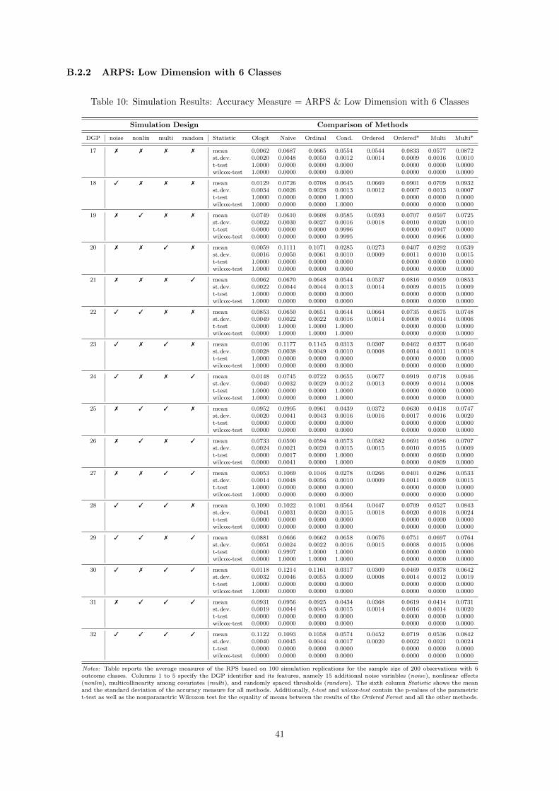
B.2.2 ARPS: Low Dimension with 6 Classes
Table 10: Simulation Results: Accuracy Measure = ARPS & Low Dimension with 6 Classes
Simulation Design Comparison of Methods
DGP noise nonlin multi random Statistic Ologit Naive Ordinal Cond. Ordered Ordered* Multi Multi*
17 7 7 7 7 mean 0.0062 0.0687 0.0665 0.0554 0.0544 0.0833 0.0577 0.0872st.dev. 0.0020 0.0048 0.0050 0.0012 0.0014 0.0009 0.0016 0.0010t-test 1.0000 0.0000 0.0000 0.0000 0.0000 0.0000 0.0000wilcox-test 1.0000 0.0000 0.0000 0.0000 0.0000 0.0000 0.0000
18 3 7 7 7 mean 0.0129 0.0726 0.0708 0.0645 0.0669 0.0901 0.0709 0.0932st.dev. 0.0034 0.0026 0.0028 0.0013 0.0012 0.0007 0.0013 0.0007t-test 1.0000 0.0000 0.0000 1.0000 0.0000 0.0000 0.0000wilcox-test 1.0000 0.0000 0.0000 1.0000 0.0000 0.0000 0.0000
19 7 3 7 7 mean 0.0749 0.0610 0.0608 0.0585 0.0593 0.0707 0.0597 0.0725st.dev. 0.0022 0.0030 0.0027 0.0016 0.0018 0.0010 0.0020 0.0010t-test 0.0000 0.0000 0.0000 0.9996 0.0000 0.0947 0.0000wilcox-test 0.0000 0.0000 0.0000 0.9995 0.0000 0.0966 0.0000
20 7 7 3 7 mean 0.0059 0.1111 0.1071 0.0285 0.0273 0.0407 0.0292 0.0539st.dev. 0.0016 0.0050 0.0061 0.0010 0.0009 0.0011 0.0010 0.0015t-test 1.0000 0.0000 0.0000 0.0000 0.0000 0.0000 0.0000wilcox-test 1.0000 0.0000 0.0000 0.0000 0.0000 0.0000 0.0000
21 7 7 7 3 mean 0.0062 0.0670 0.0648 0.0544 0.0537 0.0816 0.0569 0.0853st.dev. 0.0022 0.0044 0.0044 0.0013 0.0014 0.0009 0.0015 0.0009t-test 1.0000 0.0000 0.0000 0.0000 0.0000 0.0000 0.0000wilcox-test 1.0000 0.0000 0.0000 0.0000 0.0000 0.0000 0.0000
22 3 3 7 7 mean 0.0853 0.0650 0.0651 0.0644 0.0664 0.0735 0.0675 0.0748st.dev. 0.0049 0.0022 0.0022 0.0016 0.0014 0.0008 0.0014 0.0006t-test 0.0000 1.0000 1.0000 1.0000 0.0000 0.0000 0.0000wilcox-test 0.0000 1.0000 1.0000 1.0000 0.0000 0.0000 0.0000
23 3 7 3 7 mean 0.0106 0.1177 0.1145 0.0313 0.0307 0.0462 0.0377 0.0640st.dev. 0.0028 0.0038 0.0049 0.0010 0.0008 0.0014 0.0011 0.0018t-test 1.0000 0.0000 0.0000 0.0000 0.0000 0.0000 0.0000wilcox-test 1.0000 0.0000 0.0000 0.0000 0.0000 0.0000 0.0000
24 3 7 7 3 mean 0.0148 0.0745 0.0722 0.0655 0.0677 0.0919 0.0718 0.0946st.dev. 0.0040 0.0032 0.0029 0.0012 0.0013 0.0009 0.0014 0.0008t-test 1.0000 0.0000 0.0000 1.0000 0.0000 0.0000 0.0000wilcox-test 1.0000 0.0000 0.0000 1.0000 0.0000 0.0000 0.0000
25 7 3 3 7 mean 0.0952 0.0995 0.0961 0.0439 0.0372 0.0630 0.0418 0.0747st.dev. 0.0020 0.0041 0.0043 0.0016 0.0016 0.0017 0.0016 0.0020t-test 0.0000 0.0000 0.0000 0.0000 0.0000 0.0000 0.0000wilcox-test 0.0000 0.0000 0.0000 0.0000 0.0000 0.0000 0.0000
26 7 3 7 3 mean 0.0733 0.0590 0.0594 0.0573 0.0582 0.0691 0.0586 0.0707st.dev. 0.0024 0.0021 0.0020 0.0015 0.0015 0.0010 0.0015 0.0009t-test 0.0000 0.0017 0.0000 1.0000 0.0000 0.0660 0.0000wilcox-test 0.0000 0.0041 0.0000 1.0000 0.0000 0.0809 0.0000
27 7 7 3 3 mean 0.0053 0.1069 0.1046 0.0278 0.0266 0.0401 0.0286 0.0533st.dev. 0.0014 0.0048 0.0056 0.0010 0.0009 0.0011 0.0009 0.0015t-test 1.0000 0.0000 0.0000 0.0000 0.0000 0.0000 0.0000wilcox-test 1.0000 0.0000 0.0000 0.0000 0.0000 0.0000 0.0000
28 3 3 3 7 mean 0.1090 0.1022 0.1001 0.0564 0.0447 0.0709 0.0527 0.0843st.dev. 0.0041 0.0031 0.0030 0.0015 0.0018 0.0020 0.0018 0.0024t-test 0.0000 0.0000 0.0000 0.0000 0.0000 0.0000 0.0000wilcox-test 0.0000 0.0000 0.0000 0.0000 0.0000 0.0000 0.0000
29 3 3 7 3 mean 0.0881 0.0666 0.0662 0.0658 0.0676 0.0751 0.0697 0.0764st.dev. 0.0051 0.0024 0.0022 0.0016 0.0015 0.0008 0.0015 0.0006t-test 0.0000 0.9997 1.0000 1.0000 0.0000 0.0000 0.0000wilcox-test 0.0000 1.0000 1.0000 1.0000 0.0000 0.0000 0.0000
30 3 7 3 3 mean 0.0118 0.1214 0.1161 0.0317 0.0309 0.0469 0.0378 0.0642st.dev. 0.0032 0.0046 0.0055 0.0009 0.0008 0.0014 0.0012 0.0019t-test 1.0000 0.0000 0.0000 0.0000 0.0000 0.0000 0.0000wilcox-test 1.0000 0.0000 0.0000 0.0000 0.0000 0.0000 0.0000
31 7 3 3 3 mean 0.0931 0.0956 0.0925 0.0434 0.0368 0.0619 0.0414 0.0731st.dev. 0.0019 0.0044 0.0045 0.0015 0.0014 0.0016 0.0014 0.0020t-test 0.0000 0.0000 0.0000 0.0000 0.0000 0.0000 0.0000wilcox-test 0.0000 0.0000 0.0000 0.0000 0.0000 0.0000 0.0000
32 3 3 3 3 mean 0.1122 0.1093 0.1058 0.0574 0.0452 0.0719 0.0536 0.0842st.dev. 0.0040 0.0045 0.0044 0.0017 0.0020 0.0022 0.0021 0.0024t-test 0.0000 0.0000 0.0000 0.0000 0.0000 0.0000 0.0000wilcox-test 0.0000 0.0000 0.0000 0.0000 0.0000 0.0000 0.0000
Notes: Table reports the average measures of the RPS based on 100 simulation replications for the sample size of 200 observations with 6outcome classes. Columns 1 to 5 specify the DGP identifier and its features, namely 15 additional noise variables (noise), nonlinear effects(nonlin), multicollinearity among covariates (multi), and randomly spaced thresholds (random). The sixth column Statistic shows the meanand the standard deviation of the accuracy measure for all methods. Additionally, t-test and wilcox-test contain the p-values of the parametrict-test as well as the nonparametric Wilcoxon test for the equality of means between the results of the Ordered Forest and all the other methods.
41

B.2.3 ARPS: Low Dimension with 9 Classes
Table 11: Simulation Results: Accuracy Measure = ARPS & Low Dimension with 9 Classes
Simulation Design Comparison of Methods
DGP noise nonlin multi random Statistic Ologit Naive Ordinal Cond. Ordered Ordered* Multi Multi*
33 7 7 7 7 mean 0.0054 0.0653 0.0629 0.0528 0.0519 0.0789 0.0569 0.0850st.dev. 0.0018 0.0042 0.0042 0.0012 0.0014 0.0009 0.0017 0.0009t-test 1.0000 0.0000 0.0000 0.0000 0.0000 0.0000 0.0000wilcox-test 1.0000 0.0000 0.0000 0.0000 0.0000 0.0000 0.0000
34 3 7 7 7 mean 0.0112 0.0693 0.0672 0.0609 0.0638 0.0855 0.0704 0.0901st.dev. 0.0028 0.0027 0.0027 0.0012 0.0012 0.0007 0.0013 0.0006t-test 1.0000 0.0000 0.0000 1.0000 0.0000 0.0000 0.0000wilcox-test 1.0000 0.0000 0.0000 1.0000 0.0000 0.0000 0.0000
35 7 3 7 7 mean 0.0706 0.0573 0.0572 0.0555 0.0567 0.0669 0.0590 0.0698st.dev. 0.0023 0.0026 0.0027 0.0014 0.0015 0.0009 0.0016 0.0007t-test 0.0000 0.0220 0.0445 1.0000 0.0000 0.0000 0.0000wilcox-test 0.0000 0.0788 0.2389 1.0000 0.0000 0.0000 0.0000
36 7 7 3 7 mean 0.0052 0.1057 0.1047 0.0277 0.0263 0.0396 0.0303 0.0601st.dev. 0.0014 0.0046 0.0056 0.0009 0.0009 0.0010 0.0010 0.0014t-test 1.0000 0.0000 0.0000 0.0000 0.0000 0.0000 0.0000wilcox-test 1.0000 0.0000 0.0000 0.0000 0.0000 0.0000 0.0000
37 7 7 7 3 mean 0.0054 0.0627 0.0608 0.0518 0.0511 0.0774 0.0558 0.0835st.dev. 0.0019 0.0036 0.0035 0.0012 0.0014 0.0009 0.0016 0.0010t-test 1.0000 0.0000 0.0000 0.0001 0.0000 0.0000 0.0000wilcox-test 1.0000 0.0000 0.0000 0.0002 0.0000 0.0000 0.0000
38 3 3 7 7 mean 0.0806 0.0607 0.0608 0.0606 0.0629 0.0695 0.0661 0.0715st.dev. 0.0036 0.0016 0.0018 0.0013 0.0012 0.0008 0.0014 0.0007t-test 0.0000 1.0000 1.0000 1.0000 0.0000 0.0000 0.0000wilcox-test 0.0000 1.0000 1.0000 1.0000 0.0000 0.0000 0.0000
39 3 7 3 7 mean 0.0086 0.1122 0.1102 0.0301 0.0295 0.0443 0.0408 0.0710st.dev. 0.0017 0.0036 0.0041 0.0009 0.0008 0.0012 0.0011 0.0017t-test 1.0000 0.0000 0.0000 0.0000 0.0000 0.0000 0.0000wilcox-test 1.0000 0.0000 0.0000 0.0000 0.0000 0.0000 0.0000
40 3 7 7 3 mean 0.0106 0.0663 0.0646 0.0586 0.0615 0.0820 0.0679 0.0866st.dev. 0.0028 0.0026 0.0026 0.0011 0.0012 0.0008 0.0012 0.0007t-test 1.0000 0.0000 0.0000 1.0000 0.0000 0.0000 0.0000wilcox-test 1.0000 0.0000 0.0000 1.0000 0.0000 0.0000 0.0000
41 7 3 3 7 mean 0.0897 0.0929 0.0897 0.0417 0.0356 0.0596 0.0424 0.0776st.dev. 0.0017 0.0037 0.0038 0.0014 0.0013 0.0015 0.0014 0.0018t-test 0.0000 0.0000 0.0000 0.0000 0.0000 0.0000 0.0000wilcox-test 0.0000 0.0000 0.0000 0.0000 0.0000 0.0000 0.0000
42 7 3 7 3 mean 0.0701 0.0565 0.0564 0.0545 0.0556 0.0657 0.0579 0.0685st.dev. 0.0025 0.0024 0.0024 0.0015 0.0014 0.0008 0.0016 0.0007t-test 0.0000 0.0006 0.0010 1.0000 0.0000 0.0000 0.0000wilcox-test 0.0000 0.0028 0.0066 1.0000 0.0000 0.0000 0.0000
43 7 7 3 3 mean 0.0051 0.1034 0.1025 0.0273 0.0258 0.0394 0.0298 0.0593st.dev. 0.0015 0.0040 0.0045 0.0008 0.0007 0.0010 0.0009 0.0014t-test 1.0000 0.0000 0.0000 0.0000 0.0000 0.0000 0.0000wilcox-test 1.0000 0.0000 0.0000 0.0000 0.0000 0.0000 0.0000
44 3 3 3 7 mean 0.1018 0.0956 0.0933 0.0534 0.0432 0.0673 0.0550 0.0873st.dev. 0.0035 0.0031 0.0031 0.0013 0.0016 0.0017 0.0019 0.0021t-test 0.0000 0.0000 0.0000 0.0000 0.0000 0.0000 0.0000wilcox-test 0.0000 0.0000 0.0000 0.0000 0.0000 0.0000 0.0000
45 3 3 7 3 mean 0.0763 0.0587 0.0588 0.0582 0.0605 0.0664 0.0638 0.0684st.dev. 0.0040 0.0019 0.0018 0.0014 0.0012 0.0007 0.0011 0.0006t-test 0.0000 1.0000 1.0000 1.0000 0.0000 0.0000 0.0000wilcox-test 0.0000 1.0000 1.0000 1.0000 0.0000 0.0000 0.0000
46 3 7 3 3 mean 0.0084 0.1079 0.1066 0.0292 0.0286 0.0432 0.0391 0.0699st.dev. 0.0021 0.0034 0.0040 0.0008 0.0007 0.0012 0.0012 0.0017t-test 1.0000 0.0000 0.0000 0.0000 0.0000 0.0000 0.0000wilcox-test 1.0000 0.0000 0.0000 0.0000 0.0000 0.0000 0.0000
47 7 3 3 3 mean 0.0881 0.0915 0.0887 0.0411 0.0352 0.0588 0.0414 0.0765st.dev. 0.0017 0.0039 0.0041 0.0014 0.0012 0.0014 0.0014 0.0016t-test 0.0000 0.0000 0.0000 0.0000 0.0000 0.0000 0.0000wilcox-test 0.0000 0.0000 0.0000 0.0000 0.0000 0.0000 0.0000
48 3 3 3 3 mean 0.0973 0.0912 0.0887 0.0515 0.0421 0.0647 0.0537 0.0845st.dev. 0.0031 0.0033 0.0032 0.0015 0.0016 0.0019 0.0018 0.0017t-test 0.0000 0.0000 0.0000 0.0000 0.0000 0.0000 0.0000wilcox-test 0.0000 0.0000 0.0000 0.0000 0.0000 0.0000 0.0000
Notes: Table reports the average measures of the RPS based on 100 simulation replications for the sample size of 200 observations with 9outcome classes. Columns 1 to 5 specify the DGP identifier and its features, namely 15 additional noise variables (noise), nonlinear effects(nonlin), multicollinearity among covariates (multi), and randomly spaced thresholds (random). The sixth column Statistic shows the meanand the standard deviation of the accuracy measure for all methods. Additionally, t-test and wilcox-test contain the p-values of the parametrict-test as well as the nonparametric Wilcoxon test for the equality of means between the results of the Ordered Forest and all the other methods.
42

B.2.4 ARPS: High Dimension with 3 Classes
Table 12: Simulation Results: Accuracy Measure = ARPS & High Dimension with 3 Classes
Simulation Design Comparison of Methods
DGP noise nonlin multi random Statistic Naive Ordinal Cond. Ordered Ordered* Multi Multi*
49 3 7 7 7 mean 0.1135 0.1139 0.1112 0.1140 0.1180 0.1139 0.1179st.dev. 0.0009 0.0010 0.0009 0.0008 0.0006 0.0008 0.0006t-test 1.0000 0.7676 1.0000 0.0000 0.7268 0.0000wilcox-test 0.9999 0.8438 1.0000 0.0000 0.7191 0.0000
50 3 3 7 7 mean 0.0896 0.0899 0.0901 0.0903 0.0907 0.0901 0.0907st.dev. 0.0008 0.0010 0.0008 0.0007 0.0007 0.0007 0.0006t-test 1.0000 0.9997 0.9840 0.0002 0.9973 0.0004wilcox-test 1.0000 1.0000 0.9929 0.0000 0.9989 0.0000
51 3 7 3 7 mean 0.1534 0.1529 0.0827 0.0766 0.1082 0.0867 0.1134st.dev. 0.0011 0.0012 0.0024 0.0025 0.0029 0.0024 0.0026t-test 0.0000 0.0000 0.0000 0.0000 0.0000 0.0000wilcox-test 0.0000 0.0000 0.0000 0.0000 0.0000 0.0000
52 3 7 7 3 mean 0.1253 0.1252 0.1224 0.1248 0.1296 0.1250 0.1296st.dev. 0.0013 0.0013 0.0010 0.0009 0.0007 0.0009 0.0007t-test 0.0011 0.0115 1.0000 0.0000 0.1664 0.0000wilcox-test 0.0013 0.0140 1.0000 0.0000 0.1515 0.0000
53 3 3 3 7 mean 0.1299 0.1300 0.1048 0.1016 0.1200 0.1021 0.1202st.dev. 0.0011 0.0012 0.0034 0.0027 0.0026 0.0027 0.0025t-test 0.0000 0.0000 0.0000 0.0000 0.0674 0.0000wilcox-test 0.0000 0.0000 0.0000 0.0000 0.0494 0.0000
54 3 3 7 3 mean 0.0997 0.0996 0.0999 0.0998 0.1004 0.0997 0.1004st.dev. 0.0012 0.0013 0.0012 0.0012 0.0011 0.0011 0.0012t-test 0.5772 0.8438 0.3065 0.0000 0.6432 0.0000wilcox-test 0.6792 0.9705 0.2427 0.0000 0.7183 0.0000
55 3 7 3 3 mean 0.1678 0.1667 0.0862 0.0836 0.1167 0.0906 0.1195st.dev. 0.0015 0.0013 0.0026 0.0030 0.0029 0.0029 0.0029t-test 0.0000 0.0000 0.0000 0.0000 0.0000 0.0000wilcox-test 0.0000 0.0000 0.0000 0.0000 0.0000 0.0000
56 3 3 3 3 mean 0.1476 0.1474 0.1156 0.1102 0.1316 0.1110 0.1317st.dev. 0.0013 0.0010 0.0041 0.0029 0.0031 0.0029 0.0031t-test 0.0000 0.0000 0.0000 0.0000 0.0287 0.0000wilcox-test 0.0000 0.0000 0.0000 0.0000 0.0272 0.0000
Notes: Table reports the average measures of the RPS based on 100 simulation replications for the sample size of 200 observationswith 3 outcome classes. Columns 1 to 5 specify the DGP identifier and its features, namely 1000 additional noise variables (noise),nonlinear effects (nonlin), multicollinearity among covariates (multi), and randomly spaced thresholds (random). The sixth columnStatistic shows the mean and the standard deviation of the accuracy measure for all methods. Additionally, t-test and wilcox-testcontain the p-values of the parametric t-test as well as the nonparametric Wilcoxon test for the equality of means between the resultsof the Ordered Forest and all the other methods.
43

B.2.5 ARPS: High Dimension with 6 Classes
Table 13: Simulation Results: Accuracy Measure = ARPS & High Dimension with 6 Classes
Simulation Design Comparison of Methods
DGP noise nonlin multi random Statistic Naive Ordinal Cond. Ordered Ordered* Multi Multi*
57 3 7 7 7 mean 0.0974 0.0972 0.0951 0.0983 0.1012 0.0998 0.1016st.dev. 0.0006 0.0006 0.0006 0.0005 0.0004 0.0005 0.0004t-test 1.0000 1.0000 1.0000 0.0000 0.0000 0.0000wilcox-test 1.0000 1.0000 1.0000 0.0000 0.0000 0.0000
58 3 3 7 7 mean 0.0762 0.0762 0.0765 0.0773 0.0772 0.0776 0.0773st.dev. 0.0006 0.0006 0.0006 0.0005 0.0005 0.0004 0.0004t-test 1.0000 1.0000 1.0000 0.9803 0.0000 0.7833wilcox-test 1.0000 1.0000 1.0000 0.9838 0.0000 0.7449
59 3 7 3 7 mean 0.1336 0.1327 0.0747 0.0675 0.0968 0.0912 0.1152st.dev. 0.0008 0.0010 0.0013 0.0016 0.0015 0.0016 0.0017t-test 0.0000 0.0000 0.0000 0.0000 0.0000 0.0000wilcox-test 0.0000 0.0000 0.0000 0.0000 0.0000 0.0000
60 3 7 7 3 mean 0.0845 0.0845 0.0826 0.0857 0.0880 0.0872 0.0883st.dev. 0.0005 0.0005 0.0006 0.0004 0.0003 0.0004 0.0003t-test 1.0000 1.0000 1.0000 0.0000 0.0000 0.0000wilcox-test 1.0000 1.0000 1.0000 0.0000 0.0000 0.0000
61 3 3 3 7 mean 0.1091 0.1088 0.0891 0.0885 0.1026 0.1010 0.1105st.dev. 0.0009 0.0008 0.0025 0.0021 0.0018 0.0023 0.0010t-test 0.0000 0.0000 0.0547 0.0000 0.0000 0.0000wilcox-test 0.0000 0.0000 0.0626 0.0000 0.0000 0.0000
62 3 3 7 3 mean 0.0658 0.0659 0.0660 0.0669 0.0665 0.0672 0.0666st.dev. 0.0006 0.0006 0.0006 0.0006 0.0006 0.0005 0.0005t-test 1.0000 1.0000 1.0000 1.0000 0.0006 0.9998wilcox-test 1.0000 1.0000 1.0000 1.0000 0.0000 1.0000
63 3 7 3 3 mean 0.1167 0.1163 0.0682 0.0606 0.0872 0.0820 0.1052st.dev. 0.0007 0.0008 0.0014 0.0016 0.0015 0.0018 0.0015t-test 0.0000 0.0000 0.0000 0.0000 0.0000 0.0000wilcox-test 0.0000 0.0000 0.0000 0.0000 0.0000 0.0000
64 3 3 3 3 mean 0.0927 0.0927 0.0766 0.0772 0.0882 0.0898 0.0952st.dev. 0.0006 0.0005 0.0020 0.0016 0.0014 0.0018 0.0006t-test 0.0000 0.0000 0.9878 0.0000 0.0000 0.0000wilcox-test 0.0000 0.0000 0.9887 0.0000 0.0000 0.0000
Notes: Table reports the average measures of the RPS based on 100 simulation replications for the sample size of 200 observationswith 6 outcome classes. Columns 1 to 5 specify the DGP identifier and its features, namely 1000 additional noise variables (noise),nonlinear effects (nonlin), multicollinearity among covariates (multi), and randomly spaced thresholds (random). The sixth columnStatistic shows the mean and the standard deviation of the accuracy measure for all methods. Additionally, t-test and wilcox-testcontain the p-values of the parametric t-test as well as the nonparametric Wilcoxon test for the equality of means between the resultsof the Ordered Forest and all the other methods.
44

B.2.6 ARPS: High Dimension with 9 Classes
Table 14: Simulation Results: Accuracy Measure = ARPS & High Dimension with 9 Classes
Simulation Design Comparison of Methods
DGP noise nonlin multi random Statistic Naive Ordinal Cond. Ordered Ordered* Multi Multi*
65 3 7 7 7 mean 0.0921 0.0918 0.0900 0.0931 0.0959 0.0955 0.0964st.dev. 0.0006 0.0006 0.0006 0.0005 0.0003 0.0004 0.0003t-test 1.0000 1.0000 1.0000 0.0000 0.0000 0.0000wilcox-test 1.0000 1.0000 1.0000 0.0000 0.0000 0.0000
66 3 3 7 7 mean 0.0721 0.0720 0.0724 0.0732 0.0730 0.0739 0.0731st.dev. 0.0006 0.0005 0.0006 0.0005 0.0004 0.0004 0.0004t-test 1.0000 1.0000 1.0000 0.9959 0.0000 0.8717wilcox-test 1.0000 1.0000 1.0000 0.9991 0.0000 0.9308
67 3 7 3 7 mean 0.1268 0.1260 0.0713 0.0648 0.0926 0.0979 0.1175st.dev. 0.0008 0.0009 0.0013 0.0013 0.0014 0.0017 0.0015t-test 0.0000 0.0000 0.0000 0.0000 0.0000 0.0000wilcox-test 0.0000 0.0000 0.0000 0.0000 0.0000 0.0000
68 3 7 7 3 mean 0.0904 0.0902 0.0884 0.0915 0.0941 0.0937 0.0946st.dev. 0.0006 0.0006 0.0005 0.0005 0.0003 0.0004 0.0003t-test 1.0000 1.0000 1.0000 0.0000 0.0000 0.0000wilcox-test 1.0000 1.0000 1.0000 0.0000 0.0000 0.0000
69 3 3 3 7 mean 0.1031 0.1028 0.0838 0.0838 0.0967 0.1024 0.1061st.dev. 0.0007 0.0007 0.0021 0.0017 0.0016 0.0016 0.0005t-test 0.0000 0.0000 0.4695 0.0000 0.0000 0.0000wilcox-test 0.0000 0.0000 0.5044 0.0000 0.0000 0.0000
70 3 3 7 3 mean 0.0706 0.0707 0.0710 0.0718 0.0716 0.0724 0.0717st.dev. 0.0007 0.0007 0.0006 0.0006 0.0005 0.0005 0.0006t-test 1.0000 1.0000 1.0000 0.9903 0.0000 0.8186wilcox-test 1.0000 1.0000 1.0000 0.9983 0.0000 0.8723
71 3 7 3 3 mean 0.1246 0.1238 0.0704 0.0636 0.0911 0.0966 0.1153st.dev. 0.0007 0.0008 0.0014 0.0013 0.0014 0.0016 0.0018t-test 0.0000 0.0000 0.0000 0.0000 0.0000 0.0000wilcox-test 0.0000 0.0000 0.0000 0.0000 0.0000 0.0000
72 3 3 3 3 mean 0.1007 0.1004 0.0817 0.0819 0.0945 0.0997 0.1036st.dev. 0.0007 0.0007 0.0020 0.0017 0.0015 0.0019 0.0006t-test 0.0000 0.0000 0.7875 0.0000 0.0000 0.0000wilcox-test 0.0000 0.0000 0.8473 0.0000 0.0000 0.0000
Notes: Table reports the average measures of the RPS based on 100 simulation replications for the sample size of 200 observationswith 9 outcome classes. Columns 1 to 5 specify the DGP identifier and its features, namely 1000 additional noise variables (noise),nonlinear effects (nonlin), multicollinearity among covariates (multi), and randomly spaced thresholds (random). The sixth columnStatistic shows the mean and the standard deviation of the accuracy measure for all methods. Additionally, t-test and wilcox-testcontain the p-values of the parametric t-test as well as the nonparametric Wilcoxon test for the equality of means between the resultsof the Ordered Forest and all the other methods.
45
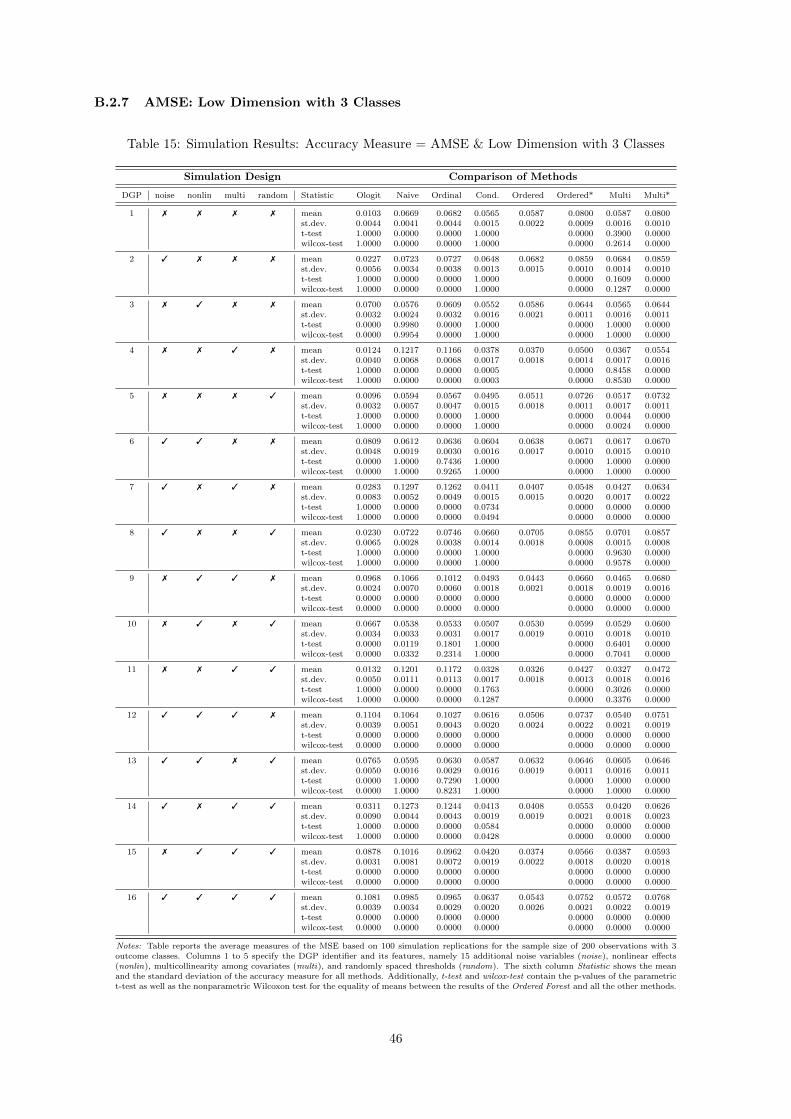
B.2.7 AMSE: Low Dimension with 3 Classes
Table 15: Simulation Results: Accuracy Measure = AMSE & Low Dimension with 3 Classes
Simulation Design Comparison of Methods
DGP noise nonlin multi random Statistic Ologit Naive Ordinal Cond. Ordered Ordered* Multi Multi*
1 7 7 7 7 mean 0.0103 0.0669 0.0682 0.0565 0.0587 0.0800 0.0587 0.0800st.dev. 0.0044 0.0041 0.0044 0.0015 0.0022 0.0009 0.0016 0.0010t-test 1.0000 0.0000 0.0000 1.0000 0.0000 0.3900 0.0000wilcox-test 1.0000 0.0000 0.0000 1.0000 0.0000 0.2614 0.0000
2 3 7 7 7 mean 0.0227 0.0723 0.0727 0.0648 0.0682 0.0859 0.0684 0.0859st.dev. 0.0056 0.0034 0.0038 0.0013 0.0015 0.0010 0.0014 0.0010t-test 1.0000 0.0000 0.0000 1.0000 0.0000 0.1609 0.0000wilcox-test 1.0000 0.0000 0.0000 1.0000 0.0000 0.1287 0.0000
3 7 3 7 7 mean 0.0700 0.0576 0.0609 0.0552 0.0586 0.0644 0.0565 0.0644st.dev. 0.0032 0.0024 0.0032 0.0016 0.0021 0.0011 0.0016 0.0011t-test 0.0000 0.9980 0.0000 1.0000 0.0000 1.0000 0.0000wilcox-test 0.0000 0.9954 0.0000 1.0000 0.0000 1.0000 0.0000
4 7 7 3 7 mean 0.0124 0.1217 0.1166 0.0378 0.0370 0.0500 0.0367 0.0554st.dev. 0.0040 0.0068 0.0068 0.0017 0.0018 0.0014 0.0017 0.0016t-test 1.0000 0.0000 0.0000 0.0005 0.0000 0.8458 0.0000wilcox-test 1.0000 0.0000 0.0000 0.0003 0.0000 0.8530 0.0000
5 7 7 7 3 mean 0.0096 0.0594 0.0567 0.0495 0.0511 0.0726 0.0517 0.0732st.dev. 0.0032 0.0057 0.0047 0.0015 0.0018 0.0011 0.0017 0.0011t-test 1.0000 0.0000 0.0000 1.0000 0.0000 0.0044 0.0000wilcox-test 1.0000 0.0000 0.0000 1.0000 0.0000 0.0024 0.0000
6 3 3 7 7 mean 0.0809 0.0612 0.0636 0.0604 0.0638 0.0671 0.0617 0.0670st.dev. 0.0048 0.0019 0.0030 0.0016 0.0017 0.0010 0.0015 0.0010t-test 0.0000 1.0000 0.7436 1.0000 0.0000 1.0000 0.0000wilcox-test 0.0000 1.0000 0.9265 1.0000 0.0000 1.0000 0.0000
7 3 7 3 7 mean 0.0283 0.1297 0.1262 0.0411 0.0407 0.0548 0.0427 0.0634st.dev. 0.0083 0.0052 0.0049 0.0015 0.0015 0.0020 0.0017 0.0022t-test 1.0000 0.0000 0.0000 0.0734 0.0000 0.0000 0.0000wilcox-test 1.0000 0.0000 0.0000 0.0494 0.0000 0.0000 0.0000
8 3 7 7 3 mean 0.0230 0.0722 0.0746 0.0660 0.0705 0.0855 0.0701 0.0857st.dev. 0.0065 0.0028 0.0038 0.0014 0.0018 0.0008 0.0015 0.0008t-test 1.0000 0.0000 0.0000 1.0000 0.0000 0.9630 0.0000wilcox-test 1.0000 0.0000 0.0000 1.0000 0.0000 0.9578 0.0000
9 7 3 3 7 mean 0.0968 0.1066 0.1012 0.0493 0.0443 0.0660 0.0465 0.0680st.dev. 0.0024 0.0070 0.0060 0.0018 0.0021 0.0018 0.0019 0.0016t-test 0.0000 0.0000 0.0000 0.0000 0.0000 0.0000 0.0000wilcox-test 0.0000 0.0000 0.0000 0.0000 0.0000 0.0000 0.0000
10 7 3 7 3 mean 0.0667 0.0538 0.0533 0.0507 0.0530 0.0599 0.0529 0.0600st.dev. 0.0034 0.0033 0.0031 0.0017 0.0019 0.0010 0.0018 0.0010t-test 0.0000 0.0119 0.1801 1.0000 0.0000 0.6401 0.0000wilcox-test 0.0000 0.0332 0.2314 1.0000 0.0000 0.7041 0.0000
11 7 7 3 3 mean 0.0132 0.1201 0.1172 0.0328 0.0326 0.0427 0.0327 0.0472st.dev. 0.0050 0.0111 0.0113 0.0017 0.0018 0.0013 0.0018 0.0016t-test 1.0000 0.0000 0.0000 0.1763 0.0000 0.3026 0.0000wilcox-test 1.0000 0.0000 0.0000 0.1287 0.0000 0.3376 0.0000
12 3 3 3 7 mean 0.1104 0.1064 0.1027 0.0616 0.0506 0.0737 0.0540 0.0751st.dev. 0.0039 0.0051 0.0043 0.0020 0.0024 0.0022 0.0021 0.0019t-test 0.0000 0.0000 0.0000 0.0000 0.0000 0.0000 0.0000wilcox-test 0.0000 0.0000 0.0000 0.0000 0.0000 0.0000 0.0000
13 3 3 7 3 mean 0.0765 0.0595 0.0630 0.0587 0.0632 0.0646 0.0605 0.0646st.dev. 0.0050 0.0016 0.0029 0.0016 0.0019 0.0011 0.0016 0.0011t-test 0.0000 1.0000 0.7290 1.0000 0.0000 1.0000 0.0000wilcox-test 0.0000 1.0000 0.8231 1.0000 0.0000 1.0000 0.0000
14 3 7 3 3 mean 0.0311 0.1273 0.1244 0.0413 0.0408 0.0553 0.0420 0.0626st.dev. 0.0090 0.0044 0.0043 0.0019 0.0019 0.0021 0.0018 0.0023t-test 1.0000 0.0000 0.0000 0.0584 0.0000 0.0000 0.0000wilcox-test 1.0000 0.0000 0.0000 0.0428 0.0000 0.0000 0.0000
15 7 3 3 3 mean 0.0878 0.1016 0.0962 0.0420 0.0374 0.0566 0.0387 0.0593st.dev. 0.0031 0.0081 0.0072 0.0019 0.0022 0.0018 0.0020 0.0018t-test 0.0000 0.0000 0.0000 0.0000 0.0000 0.0000 0.0000wilcox-test 0.0000 0.0000 0.0000 0.0000 0.0000 0.0000 0.0000
16 3 3 3 3 mean 0.1081 0.0985 0.0965 0.0637 0.0543 0.0752 0.0572 0.0768st.dev. 0.0039 0.0034 0.0029 0.0020 0.0026 0.0021 0.0022 0.0019t-test 0.0000 0.0000 0.0000 0.0000 0.0000 0.0000 0.0000wilcox-test 0.0000 0.0000 0.0000 0.0000 0.0000 0.0000 0.0000
Notes: Table reports the average measures of the MSE based on 100 simulation replications for the sample size of 200 observations with 3outcome classes. Columns 1 to 5 specify the DGP identifier and its features, namely 15 additional noise variables (noise), nonlinear effects(nonlin), multicollinearity among covariates (multi), and randomly spaced thresholds (random). The sixth column Statistic shows the meanand the standard deviation of the accuracy measure for all methods. Additionally, t-test and wilcox-test contain the p-values of the parametrict-test as well as the nonparametric Wilcoxon test for the equality of means between the results of the Ordered Forest and all the other methods.
46

B.2.8 AMSE: Low Dimension with 6 Classes
Table 16: Simulation Results: Accuracy Measure = AMSE & Low Dimension with 6 Classes
Simulation Design Comparison of Methods
DGP noise nonlin multi random Statistic Ologit Naive Ordinal Cond. Ordered Ordered* Multi Multi*
17 7 7 7 7 mean 0.0043 0.0284 0.0283 0.0248 0.0291 0.0324 0.0287 0.0327st.dev. 0.0014 0.0012 0.0018 0.0007 0.0010 0.0005 0.0008 0.0005t-test 1.0000 1.0000 0.9998 1.0000 0.0000 0.9958 0.0000wilcox-test 1.0000 1.0000 1.0000 1.0000 0.0000 0.9953 0.0000
18 3 7 7 7 mean 0.0083 0.0294 0.0292 0.0272 0.0311 0.0337 0.0310 0.0341st.dev. 0.0021 0.0007 0.0010 0.0005 0.0006 0.0003 0.0005 0.0003t-test 1.0000 1.0000 1.0000 1.0000 0.0000 0.9791 0.0000wilcox-test 1.0000 1.0000 1.0000 1.0000 0.0000 0.9805 0.0000
19 7 3 7 7 mean 0.0245 0.0216 0.0222 0.0207 0.0257 0.0237 0.0240 0.0237st.dev. 0.0007 0.0009 0.0009 0.0006 0.0009 0.0004 0.0008 0.0004t-test 1.0000 1.0000 1.0000 1.0000 1.0000 1.0000 1.0000wilcox-test 1.0000 1.0000 1.0000 1.0000 1.0000 1.0000 1.0000
20 7 7 3 7 mean 0.0065 0.0600 0.0568 0.0238 0.0259 0.0299 0.0263 0.0356st.dev. 0.0017 0.0019 0.0023 0.0008 0.0009 0.0007 0.0008 0.0007t-test 1.0000 0.0000 0.0000 1.0000 0.0000 0.0006 0.0000wilcox-test 1.0000 0.0000 0.0000 1.0000 0.0000 0.0002 0.0000
21 7 7 7 3 mean 0.0043 0.0283 0.0282 0.0248 0.0291 0.0324 0.0289 0.0327st.dev. 0.0014 0.0013 0.0015 0.0007 0.0009 0.0005 0.0007 0.0005t-test 1.0000 1.0000 1.0000 1.0000 0.0000 0.9689 0.0000wilcox-test 1.0000 1.0000 1.0000 1.0000 0.0000 0.9661 0.0000
22 3 3 7 7 mean 0.0273 0.0223 0.0228 0.0220 0.0263 0.0242 0.0249 0.0243st.dev. 0.0015 0.0007 0.0008 0.0005 0.0007 0.0004 0.0006 0.0003t-test 0.0000 1.0000 1.0000 1.0000 1.0000 1.0000 1.0000wilcox-test 0.0000 1.0000 1.0000 1.0000 1.0000 1.0000 1.0000
23 3 7 3 7 mean 0.0114 0.0607 0.0580 0.0258 0.0266 0.0319 0.0305 0.0396st.dev. 0.0030 0.0014 0.0017 0.0007 0.0007 0.0008 0.0008 0.0007t-test 1.0000 0.0000 0.0000 1.0000 0.0000 0.0000 0.0000wilcox-test 1.0000 0.0000 0.0000 1.0000 0.0000 0.0000 0.0000
24 3 7 7 3 mean 0.0088 0.0306 0.0296 0.0274 0.0306 0.0346 0.0310 0.0350st.dev. 0.0023 0.0010 0.0011 0.0005 0.0006 0.0004 0.0006 0.0004t-test 1.0000 0.6721 1.0000 1.0000 0.0000 0.0000 0.0000wilcox-test 1.0000 0.3992 1.0000 1.0000 0.0000 0.0000 0.0000
25 7 3 3 7 mean 0.0374 0.0396 0.0377 0.0234 0.0256 0.0292 0.0254 0.0315st.dev. 0.0007 0.0016 0.0013 0.0008 0.0011 0.0008 0.0009 0.0007t-test 0.0000 0.0000 0.0000 1.0000 0.0000 0.9637 0.0000wilcox-test 0.0000 0.0000 0.0000 1.0000 0.0000 0.9567 0.0000
26 7 3 7 3 mean 0.0245 0.0215 0.0224 0.0207 0.0256 0.0236 0.0241 0.0237st.dev. 0.0008 0.0007 0.0009 0.0006 0.0008 0.0004 0.0007 0.0005t-test 1.0000 1.0000 1.0000 1.0000 1.0000 1.0000 1.0000wilcox-test 1.0000 1.0000 1.0000 1.0000 1.0000 1.0000 1.0000
27 7 7 3 3 mean 0.0060 0.0587 0.0560 0.0236 0.0254 0.0297 0.0262 0.0355st.dev. 0.0015 0.0017 0.0019 0.0007 0.0009 0.0007 0.0009 0.0007t-test 1.0000 0.0000 0.0000 1.0000 0.0000 0.0000 0.0000wilcox-test 1.0000 0.0000 0.0000 1.0000 0.0000 0.0000 0.0000
28 3 3 3 7 mean 0.0416 0.0396 0.0384 0.0271 0.0272 0.0312 0.0280 0.0338st.dev. 0.0014 0.0012 0.0009 0.0006 0.0009 0.0008 0.0008 0.0006t-test 0.0000 0.0000 0.0000 0.8880 0.0000 0.0000 0.0000wilcox-test 0.0000 0.0000 0.0000 0.8212 0.0000 0.0000 0.0000
29 3 3 7 3 mean 0.0292 0.0239 0.0240 0.0231 0.0268 0.0255 0.0261 0.0256st.dev. 0.0016 0.0009 0.0008 0.0005 0.0007 0.0003 0.0005 0.0003t-test 0.0000 1.0000 1.0000 1.0000 1.0000 1.0000 1.0000wilcox-test 0.0000 1.0000 1.0000 1.0000 1.0000 1.0000 1.0000
30 3 7 3 3 mean 0.0115 0.0618 0.0580 0.0242 0.0246 0.0306 0.0285 0.0375st.dev. 0.0029 0.0018 0.0020 0.0006 0.0006 0.0007 0.0008 0.0006t-test 1.0000 0.0000 0.0000 0.9999 0.0000 0.0000 0.0000wilcox-test 1.0000 0.0000 0.0000 0.9999 0.0000 0.0000 0.0000
31 7 3 3 3 mean 0.0378 0.0394 0.0375 0.0236 0.0256 0.0295 0.0256 0.0317st.dev. 0.0008 0.0014 0.0013 0.0007 0.0009 0.0007 0.0008 0.0006t-test 0.0000 0.0000 0.0000 1.0000 0.0000 0.6494 0.0000wilcox-test 0.0000 0.0000 0.0000 1.0000 0.0000 0.6416 0.0000
32 3 3 3 3 mean 0.0433 0.0438 0.0413 0.0270 0.0260 0.0314 0.0274 0.0339st.dev. 0.0014 0.0017 0.0014 0.0008 0.0011 0.0009 0.0010 0.0008t-test 0.0000 0.0000 0.0000 0.0000 0.0000 0.0000 0.0000wilcox-test 0.0000 0.0000 0.0000 0.0000 0.0000 0.0000 0.0000
Notes: Table reports the average measures of the MSE based on 100 simulation replications for the sample size of 200 observations with 6outcome classes. Columns 1 to 5 specify the DGP identifier and its features, namely 15 additional noise variables (noise), nonlinear effects(nonlin), multicollinearity among covariates (multi), and randomly spaced thresholds (random). The sixth column Statistic shows the meanand the standard deviation of the accuracy measure for all methods. Additionally, t-test and wilcox-test contain the p-values of the parametrict-test as well as the nonparametric Wilcoxon test for the equality of means between the results of the Ordered Forest and all the other methods.
47

B.2.9 AMSE: Low Dimension with 9 Classes
Table 17: Simulation Results: Accuracy Measure = AMSE & Low Dimension with 9 Classes
Simulation Design Comparison of Methods
DGP noise nonlin multi random Statistic Ologit Naive Ordinal Cond. Ordered Ordered* Multi Multi*
33 7 7 7 7 mean 0.0025 0.0150 0.0149 0.0134 0.0170 0.0170 0.0168 0.0172st.dev. 0.0008 0.0005 0.0007 0.0004 0.0006 0.0003 0.0005 0.0002t-test 1.0000 1.0000 1.0000 1.0000 0.5492 0.9993 0.0040wilcox-test 1.0000 1.0000 1.0000 1.0000 0.3269 0.9985 0.0003
34 3 7 7 7 mean 0.0046 0.0155 0.0154 0.0144 0.0176 0.0175 0.0175 0.0178st.dev. 0.0011 0.0004 0.0004 0.0003 0.0004 0.0002 0.0003 0.0002t-test 1.0000 1.0000 1.0000 1.0000 0.9697 0.9696 0.0011wilcox-test 1.0000 1.0000 1.0000 1.0000 0.9359 0.9544 0.0003
35 7 3 7 7 mean 0.0123 0.0110 0.0114 0.0107 0.0147 0.0121 0.0137 0.0121st.dev. 0.0004 0.0004 0.0005 0.0004 0.0006 0.0003 0.0005 0.0003t-test 1.0000 1.0000 1.0000 1.0000 1.0000 1.0000 1.0000wilcox-test 1.0000 1.0000 1.0000 1.0000 1.0000 1.0000 1.0000
36 7 7 3 7 mean 0.0044 0.0333 0.0321 0.0148 0.0168 0.0185 0.0175 0.0222st.dev. 0.0010 0.0008 0.0009 0.0004 0.0005 0.0005 0.0005 0.0003t-test 1.0000 0.0000 0.0000 1.0000 0.0000 0.0000 0.0000wilcox-test 1.0000 0.0000 0.0000 1.0000 0.0000 0.0000 0.0000
37 7 7 7 3 mean 0.0026 0.0152 0.0154 0.0136 0.0173 0.0172 0.0170 0.0175st.dev. 0.0009 0.0005 0.0006 0.0003 0.0006 0.0002 0.0004 0.0002t-test 1.0000 1.0000 1.0000 1.0000 0.8591 1.0000 0.0034wilcox-test 1.0000 1.0000 1.0000 1.0000 0.7952 1.0000 0.0032
38 3 3 7 7 mean 0.0136 0.0112 0.0115 0.0111 0.0144 0.0122 0.0137 0.0122st.dev. 0.0006 0.0003 0.0004 0.0003 0.0004 0.0002 0.0003 0.0002t-test 1.0000 1.0000 1.0000 1.0000 1.0000 1.0000 1.0000wilcox-test 1.0000 1.0000 1.0000 1.0000 1.0000 1.0000 1.0000
39 3 7 3 7 mean 0.0066 0.0335 0.0323 0.0159 0.0167 0.0192 0.0200 0.0242st.dev. 0.0012 0.0006 0.0007 0.0005 0.0005 0.0006 0.0005 0.0004t-test 1.0000 0.0000 0.0000 1.0000 0.0000 0.0000 0.0000wilcox-test 1.0000 0.0000 0.0000 1.0000 0.0000 0.0000 0.0000
40 3 7 7 3 mean 0.0046 0.0152 0.0152 0.0142 0.0175 0.0172 0.0173 0.0174st.dev. 0.0011 0.0004 0.0005 0.0003 0.0004 0.0002 0.0003 0.0002t-test 1.0000 1.0000 1.0000 1.0000 1.0000 0.9998 0.9655wilcox-test 1.0000 1.0000 1.0000 1.0000 1.0000 0.9999 0.9525
41 7 3 3 7 mean 0.0190 0.0198 0.0192 0.0127 0.0158 0.0156 0.0152 0.0170st.dev. 0.0004 0.0007 0.0007 0.0004 0.0006 0.0004 0.0005 0.0003t-test 0.0000 0.0000 0.0000 1.0000 0.9652 1.0000 0.0000wilcox-test 0.0000 0.0000 0.0000 1.0000 0.9503 1.0000 0.0000
42 7 3 7 3 mean 0.0125 0.0112 0.0117 0.0108 0.0147 0.0122 0.0138 0.0122st.dev. 0.0004 0.0004 0.0007 0.0003 0.0005 0.0002 0.0005 0.0002t-test 1.0000 1.0000 1.0000 1.0000 1.0000 1.0000 1.0000wilcox-test 1.0000 1.0000 1.0000 1.0000 1.0000 1.0000 1.0000
43 7 7 3 3 mean 0.0043 0.0335 0.0324 0.0149 0.0167 0.0187 0.0176 0.0225st.dev. 0.0013 0.0007 0.0009 0.0005 0.0005 0.0005 0.0005 0.0004t-test 1.0000 0.0000 0.0000 1.0000 0.0000 0.0000 0.0000wilcox-test 1.0000 0.0000 0.0000 1.0000 0.0000 0.0000 0.0000
44 3 3 3 7 mean 0.0208 0.0198 0.0193 0.0143 0.0159 0.0164 0.0162 0.0181st.dev. 0.0007 0.0006 0.0005 0.0003 0.0006 0.0004 0.0005 0.0003t-test 0.0000 0.0000 0.0000 1.0000 0.0000 0.0001 0.0000wilcox-test 0.0000 0.0000 0.0000 1.0000 0.0000 0.0000 0.0000
45 3 3 7 3 mean 0.0130 0.0110 0.0113 0.0108 0.0142 0.0118 0.0134 0.0118st.dev. 0.0006 0.0003 0.0003 0.0003 0.0004 0.0003 0.0003 0.0002t-test 1.0000 1.0000 1.0000 1.0000 1.0000 1.0000 1.0000wilcox-test 1.0000 1.0000 1.0000 1.0000 1.0000 1.0000 1.0000
46 3 7 3 3 mean 0.0070 0.0335 0.0325 0.0166 0.0173 0.0200 0.0204 0.0250st.dev. 0.0016 0.0005 0.0007 0.0004 0.0005 0.0005 0.0005 0.0004t-test 1.0000 0.0000 0.0000 1.0000 0.0000 0.0000 0.0000wilcox-test 1.0000 0.0000 0.0000 1.0000 0.0000 0.0000 0.0000
47 7 3 3 3 mean 0.0192 0.0203 0.0198 0.0130 0.0159 0.0158 0.0153 0.0173st.dev. 0.0004 0.0007 0.0007 0.0004 0.0006 0.0004 0.0005 0.0003t-test 0.0000 0.0000 0.0000 1.0000 0.6681 1.0000 0.0000wilcox-test 0.0000 0.0000 0.0000 1.0000 0.5336 1.0000 0.0000
48 3 3 3 3 mean 0.0203 0.0194 0.0190 0.0142 0.0159 0.0161 0.0162 0.0179st.dev. 0.0006 0.0006 0.0005 0.0003 0.0005 0.0003 0.0004 0.0003t-test 0.0000 0.0000 0.0000 1.0000 0.0006 0.0000 0.0000wilcox-test 0.0000 0.0000 0.0000 1.0000 0.0004 0.0000 0.0000
Notes: Table reports the average measures of the MSE based on 100 simulation replications for the sample size of 200 observations with 9outcome classes. Columns 1 to 5 specify the DGP identifier and its features, namely 15 additional noise variables (noise), nonlinear effects(nonlin), multicollinearity among covariates (multi), and randomly spaced thresholds (random). The sixth column Statistic shows the meanand the standard deviation of the accuracy measure for all methods. Additionally, t-test and wilcox-test contain the p-values of the parametrict-test as well as the nonparametric Wilcoxon test for the equality of means between the results of the Ordered Forest and all the other methods.
48

B.2.10 AMSE: High Dimension with 3 Classes
Table 18: Simulation Results: Accuracy Measure = AMSE & High Dimension with 3 Classes
Simulation Design Comparison of Methods
DGP noise nonlin multi random Statistic Naive Ordinal Cond. Ordered Ordered* Multi Multi*
49 3 7 7 7 mean 0.0923 0.0931 0.0908 0.0930 0.0952 0.0926 0.0952st.dev. 0.0008 0.0013 0.0009 0.0009 0.0007 0.0007 0.0007t-test 1.0000 0.2408 1.0000 0.0000 0.9980 0.0000wilcox-test 1.0000 0.5433 1.0000 0.0000 0.9977 0.0000
50 3 3 7 7 mean 0.0692 0.0698 0.0696 0.0702 0.0699 0.0696 0.0699st.dev. 0.0009 0.0013 0.0010 0.0009 0.0009 0.0008 0.0008t-test 1.0000 0.9907 0.9999 0.9649 1.0000 0.9852wilcox-test 1.0000 1.0000 1.0000 0.9887 1.0000 0.9944
51 3 7 3 7 mean 0.1385 0.1379 0.0864 0.0752 0.1008 0.0881 0.1087st.dev. 0.0009 0.0010 0.0019 0.0021 0.0023 0.0019 0.0018t-test 0.0000 0.0000 0.0000 0.0000 0.0000 0.0000wilcox-test 0.0000 0.0000 0.0000 0.0000 0.0000 0.0000
52 3 7 7 3 mean 0.0906 0.0904 0.0884 0.0902 0.0931 0.0902 0.0931st.dev. 0.0011 0.0013 0.0008 0.0008 0.0007 0.0008 0.0007t-test 0.0006 0.0794 1.0000 0.0000 0.3296 0.0000wilcox-test 0.0010 0.1853 1.0000 0.0000 0.2606 0.0000
53 3 3 3 7 mean 0.1079 0.1083 0.0910 0.0888 0.1010 0.0892 0.1013st.dev. 0.0009 0.0011 0.0025 0.0020 0.0019 0.0019 0.0019t-test 0.0000 0.0000 0.0000 0.0000 0.0936 0.0000wilcox-test 0.0000 0.0000 0.0000 0.0000 0.0745 0.0000
54 3 3 7 3 mean 0.0706 0.0703 0.0703 0.0705 0.0706 0.0704 0.0706st.dev. 0.0010 0.0011 0.0010 0.0009 0.0009 0.0008 0.0009t-test 0.1479 0.9409 0.8941 0.1495 0.7655 0.1796wilcox-test 0.1712 0.9972 0.9496 0.0718 0.8048 0.1178
55 3 7 3 3 mean 0.1291 0.1276 0.0725 0.0678 0.0914 0.0758 0.0954st.dev. 0.0016 0.0010 0.0020 0.0021 0.0021 0.0020 0.0020t-test 0.0000 0.0000 0.0000 0.0000 0.0000 0.0000wilcox-test 0.0000 0.0000 0.0000 0.0000 0.0000 0.0000
56 3 3 3 3 mean 0.1081 0.1079 0.0863 0.0828 0.0970 0.0834 0.0971st.dev. 0.0012 0.0009 0.0028 0.0019 0.0021 0.0020 0.0021t-test 0.0000 0.0000 0.0000 0.0000 0.0264 0.0000wilcox-test 0.0000 0.0000 0.0000 0.0000 0.0364 0.0000
Notes: Table reports the average measures of the MSE based on 100 simulation replications for the sample size of 200 observationswith 3 outcome classes. Columns 1 to 5 specify the DGP identifier and its features, namely 1000 additional noise variables (noise),nonlinear effects (nonlin), multicollinearity among covariates (multi), and randomly spaced thresholds (random). The sixth columnStatistic shows the mean and the standard deviation of the accuracy measure for all methods. Additionally, t-test and wilcox-testcontain the p-values of the parametric t-test as well as the nonparametric Wilcoxon test for the equality of means between the resultsof the Ordered Forest and all the other methods.
49

B.2.11 AMSE: High Dimension with 6 Classes
Table 19: Simulation Results: Accuracy Measure = AMSE & High Dimension with 6 Classes
Simulation Design Comparison of Methods
DGP noise nonlin multi random Statistic Naive Ordinal Cond. Ordered Ordered* Multi Multi*
57 3 7 7 7 mean 0.0352 0.0352 0.0347 0.0361 0.0361 0.0360 0.0361st.dev. 0.0003 0.0004 0.0004 0.0004 0.0004 0.0003 0.0004t-test 1.0000 1.0000 1.0000 0.8112 0.9994 0.6394wilcox-test 1.0000 1.0000 1.0000 0.8788 0.9989 0.6579
58 3 3 7 7 mean 0.0246 0.0246 0.0246 0.0257 0.0248 0.0252 0.0248st.dev. 0.0003 0.0003 0.0003 0.0004 0.0003 0.0002 0.0003t-test 1.0000 1.0000 1.0000 1.0000 1.0000 1.0000wilcox-test 1.0000 1.0000 1.0000 1.0000 1.0000 1.0000
59 3 7 3 7 mean 0.0622 0.0617 0.0459 0.0383 0.0494 0.0479 0.0553st.dev. 0.0003 0.0003 0.0005 0.0007 0.0007 0.0006 0.0006t-test 0.0000 0.0000 0.0000 0.0000 0.0000 0.0000wilcox-test 0.0000 0.0000 0.0000 0.0000 0.0000 0.0000
60 3 7 7 3 mean 0.0339 0.0341 0.0335 0.0350 0.0347 0.0348 0.0348st.dev. 0.0003 0.0004 0.0004 0.0004 0.0004 0.0003 0.0004t-test 1.0000 1.0000 1.0000 1.0000 0.9993 0.9999wilcox-test 1.0000 1.0000 1.0000 1.0000 0.9995 1.0000
61 3 3 3 7 mean 0.0397 0.0397 0.0351 0.0358 0.0383 0.0380 0.0399st.dev. 0.0004 0.0004 0.0007 0.0006 0.0005 0.0006 0.0004t-test 0.0000 0.0000 1.0000 0.0000 0.0000 0.0000wilcox-test 0.0000 0.0000 1.0000 0.0000 0.0000 0.0000
62 3 3 7 3 mean 0.0229 0.0231 0.0229 0.0241 0.0231 0.0235 0.0231st.dev. 0.0004 0.0005 0.0005 0.0005 0.0005 0.0004 0.0005t-test 1.0000 1.0000 1.0000 1.0000 1.0000 1.0000wilcox-test 1.0000 1.0000 1.0000 1.0000 1.0000 1.0000
63 3 7 3 3 mean 0.0628 0.0629 0.0481 0.0405 0.0512 0.0506 0.0583st.dev. 0.0003 0.0004 0.0005 0.0008 0.0007 0.0006 0.0005t-test 0.0000 0.0000 0.0000 0.0000 0.0000 0.0000wilcox-test 0.0000 0.0000 0.0000 0.0000 0.0000 0.0000
64 3 3 3 3 mean 0.0383 0.0386 0.0343 0.0350 0.0367 0.0378 0.0387st.dev. 0.0003 0.0004 0.0006 0.0005 0.0005 0.0005 0.0004t-test 0.0000 0.0000 1.0000 0.0000 0.0000 0.0000wilcox-test 0.0000 0.0000 1.0000 0.0000 0.0000 0.0000
Notes: Table reports the average measures of the MSE based on 100 simulation replications for the sample size of 200 observationswith 6 outcome classes. Columns 1 to 5 specify the DGP identifier and its features, namely 1000 additional noise variables (noise),nonlinear effects (nonlin), multicollinearity among covariates (multi), and randomly spaced thresholds (random). The sixth columnStatistic shows the mean and the standard deviation of the accuracy measure for all methods. Additionally, t-test and wilcox-testcontain the p-values of the parametric t-test as well as the nonparametric Wilcoxon test for the equality of means between the resultsof the Ordered Forest and all the other methods.
50

B.2.12 AMSE: High Dimension with 9 Classes
Table 20: Simulation Results: Accuracy Measure = AMSE & High Dimension with 9 Classes
Simulation Design Comparison of Methods
DGP noise nonlin multi random Statistic Naive Ordinal Cond. Ordered Ordered* Multi Multi*
65 3 7 7 7 mean 0.0180 0.0181 0.0178 0.0189 0.0185 0.0188 0.0185st.dev. 0.0002 0.0002 0.0002 0.0002 0.0002 0.0002 0.0002t-test 1.0000 1.0000 1.0000 1.0000 1.0000 1.0000wilcox-test 1.0000 1.0000 1.0000 1.0000 1.0000 1.0000
66 3 3 7 7 mean 0.0123 0.0123 0.0123 0.0133 0.0124 0.0129 0.0124st.dev. 0.0002 0.0002 0.0002 0.0002 0.0002 0.0002 0.0002t-test 1.0000 1.0000 1.0000 1.0000 1.0000 1.0000wilcox-test 1.0000 1.0000 1.0000 1.0000 1.0000 1.0000
67 3 7 3 7 mean 0.0339 0.0337 0.0263 0.0224 0.0281 0.0284 0.0316st.dev. 0.0002 0.0002 0.0003 0.0005 0.0004 0.0003 0.0003t-test 0.0000 0.0000 0.0000 0.0000 0.0000 0.0000wilcox-test 0.0000 0.0000 0.0000 0.0000 0.0000 0.0000
68 3 7 7 3 mean 0.0181 0.0181 0.0179 0.0190 0.0186 0.0188 0.0186st.dev. 0.0002 0.0002 0.0003 0.0003 0.0003 0.0002 0.0003t-test 1.0000 1.0000 1.0000 1.0000 1.0000 1.0000wilcox-test 1.0000 1.0000 1.0000 1.0000 1.0000 1.0000
69 3 3 3 7 mean 0.0198 0.0199 0.0178 0.0187 0.0193 0.0201 0.0201st.dev. 0.0002 0.0002 0.0003 0.0003 0.0003 0.0002 0.0002t-test 0.0000 0.0000 1.0000 0.0000 0.0000 0.0000wilcox-test 0.0000 0.0000 1.0000 0.0000 0.0000 0.0000
70 3 3 7 3 mean 0.0124 0.0124 0.0124 0.0133 0.0125 0.0130 0.0125st.dev. 0.0002 0.0002 0.0002 0.0003 0.0002 0.0002 0.0002t-test 1.0000 1.0000 1.0000 1.0000 1.0000 1.0000wilcox-test 1.0000 1.0000 1.0000 1.0000 1.0000 1.0000
71 3 7 3 3 mean 0.0338 0.0337 0.0262 0.0225 0.0281 0.0285 0.0315st.dev. 0.0002 0.0002 0.0004 0.0005 0.0005 0.0003 0.0004t-test 0.0000 0.0000 0.0000 0.0000 0.0000 0.0000wilcox-test 0.0000 0.0000 0.0000 0.0000 0.0000 0.0000
72 3 3 3 3 mean 0.0200 0.0200 0.0178 0.0187 0.0193 0.0201 0.0202st.dev. 0.0002 0.0002 0.0003 0.0003 0.0003 0.0003 0.0002t-test 0.0000 0.0000 1.0000 0.0000 0.0000 0.0000wilcox-test 0.0000 0.0000 1.0000 0.0000 0.0000 0.0000
Notes: Table reports the average measures of the MSE based on 100 simulation replications for the sample size of 200 observationswith 9 outcome classes. Columns 1 to 5 specify the DGP identifier and its features, namely 1000 additional noise variables (noise),nonlinear effects (nonlin), multicollinearity among covariates (multi), and randomly spaced thresholds (random). The sixth columnStatistic shows the mean and the standard deviation of the accuracy measure for all methods. Additionally, t-test and wilcox-testcontain the p-values of the parametric t-test as well as the nonparametric Wilcoxon test for the equality of means between the resultsof the Ordered Forest and all the other methods.
51

B.3 Software Implementation
The Monte Carlo study has been conducted using the R statistical software (R Core Team, 2018)
in version 3.5.2 (Eggshell Igloo) and the respective packages implementing the estimators used. With
regards to the forest-based estimators the main tuning parameters, namely the number of trees, the
number of randomly chosen covariates and the minimum leaf size have been specified according to the
values in Table 1.
Table 21: Overview of Software Packages and Tuning Parameters
Software Implementation and Tuning Parameters
method Ologit Naive Ordinal Conditional Ordered Ordered* Multi Multi*package rms ordinalForest ordinalForest party ranger grf ranger grffunction lrm ordfor ordfor cforest ranger regression forest ranger regression forest
max. iterations 25 - - - - - - -trees - 1000 1000 1000 1000 1000 1000 1000random subset -
√p
√p
√p
√p
√p
√p
√p
leaf size - 5 5 0 5 5 5 5Bsets - 1000 - - - - - -Bprior - 100 - - - - - -performance - equal - - - - - -Sbest - 10 - - - - - -
In terms of the particular R packages used the ordered logistic regression has been implemented
using the rms package (version 5.1-3) written by Harrell (2019). The respective lrm function for fitting
the ordered logit has been used with the default parameters, except setting the maximum number of
iterations, maxit=25 as for some of the DGPs the ordered logit has experienced convergence issues. Next,
the naive and the ordinal forest have been applied based on the ordinalForest package in version 2.3
(Hornung, 2019b) with the ordfor function. As described in Appendix A.3 the ordinal forest introduces
additional tuning parameters for which we use the default parameters as suggested in the package manual.
Further, the conditional forest has been estimated with the package party in version 1.3-1 (Hothorn,
Buhlmann, Dudoit, Molinaro, and Van Der Laan, 2006a; Strobl, Boulesteix, Zeileis, and Hothorn, 2007;
Strobl, Boulesteix, Kneib, Augustin, and Zeileis, 2008). Regarding the choice of the tuning parameters,
we rely on the default parameters of the cforest function. A particularity of the conditional forest is, due
to the conceptual differences to standard regression forest in terms of the splitting criterion, the choice of
the stopping rule. This is controlled by the significance level α (see Appendix A.2 for details). However,
in order to grow deep trees we follow the suggestion in the package manual to set mincriterion= 0, which
has been also used in the simulation study conducted in Janitza et al. (2016). Lastly, the Ordered
Forest as well as the multinomial forest algorithms are implemented using the package ranger in version
0.11.1 (Wright and Ziegler, 2017) with the default hyperparameters. The honest versions of the above
two estimators rely on the grf package in version 0.10.2 (Tibshirani, Athey, Wager, Friedberg, Miner,
and Wright, 2018) with the default hyperparameters as well. A detailed overview of packages with the
corresponding tuning parameters is provided in Table 21.
Furthermore, Tables 22 and 23 compare the absolute and relative computation time of the respec-
tive methods. For comparison purposes, we measure the computation time for the four main DGPs
presented in Section 5.3, namely the simple DGP in the low- and high-dimensional case as well as the
complex DGP in the low- and high-dimensional case, for both the small sample size (N = 200) and the
big sample size (N = 800) for all considered number of outcome classes. We estimate the model based
on the training set and predict the class probabilities for a test set of size N = 10000 as in the main
simulation. We repeat this procedure 10 times and report the average computation time. The tuning
52

parameters and the software implementations are chosen as defined in Tables 1 and 21, respectively. All
simulations are computed on a 64-Bit Windows machine with 4 cores (1.80GHz) and 16GB RAM storage.
Table 22: Absolute Computation Time in Seconds
Simulation Design Comparison of Methods
Class Dim. DGP Size Ologit Naive Ordinal Cond. Ordered Ordered* Multi Multi*
3 Low Simple 200 0.01 1.22 10.33 46.61 0.62 1.24 0.91 1.863 Low Simple 800 0.02 1.58 40.83 150.84 1.03 1.96 1.61 2.983 Low Complex 200 0.02 1.19 11.93 47.43 0.63 1.26 0.98 1.923 Low Complex 800 0.03 1.71 52.45 150.59 1.08 1.94 1.73 3.06
3 High Simple 200 3.50 61.89 64.28 4.05 5.08 6.06 7.273 High Simple 800 13.91 332.60 175.76 7.19 7.10 12.19 11.023 High Complex 200 3.46 60.25 59.98 4.02 4.96 6.02 7.103 High Complex 800 13.83 325.65 173.63 6.83 6.61 11.50 10.66
6 Low Simple 200 0.02 1.88 12.79 46.80 1.47 3.00 1.74 3.526 Low Simple 800 0.03 2.28 48.98 151.58 2.45 4.75 3.10 5.826 Low Complex 200 0.03 1.85 14.75 46.97 1.56 3.12 1.85 3.666 Low Complex 800 0.04 2.54 64.44 151.84 2.68 4.82 3.30 6.02
6 High Simple 200 4.21 69.80 64.14 10.24 11.74 12.01 13.636 High Simple 800 15.86 386.02 176.27 19.34 17.43 26.24 19.976 High Complex 200 4.11 70.51 60.85 9.98 11.52 11.95 13.616 High Complex 800 15.85 371.69 174.17 18.11 17.18 24.43 19.52
9 Low Simple 200 0.03 2.32 20.53 46.70 2.27 4.71 2.44 5.039 Low Simple 800 0.04 2.69 57.22 145.21 3.82 7.29 4.61 7.999 Low Complex 200 0.03 2.29 22.86 47.36 2.40 4.83 2.65 5.289 Low Complex 800 0.05 3.07 79.15 151.36 4.27 7.75 5.81 8.68
9 High Simple 200 4.85 80.76 63.25 16.05 17.84 17.69 19.569 High Simple 800 16.91 413.74 169.91 31.34 26.91 38.95 27.389 High Complex 200 4.62 78.86 57.68 15.79 17.78 17.57 19.599 High Complex 800 18.10 437.04 175.07 31.12 27.33 37.59 28.16
Notes: Table reports the average absolute computation time in seconds based on 10 simulation replications of training and prediction.The first column denotes the number of outcome classes. Columns 2 and 3 specify the dimension and the DGP, respectively. Thefourth column contains the number of observations in the training set. The prediction set consists of 10 000 observations.
The results reveal the expected pattern for the Ordered Forest. The more outcome classes the longer
the computation time as by definition of the algorithm more forests have to be estimated. Furthermore,
we also observe a longer computation time if the number of observation and/or the number of considered
splitting covariates increases which is also an expected behaviour. However, the computation time is not
sensitive to the particular DGP which it should not be either. The latter two patterns are true for all
considered methods. In comparison to the other forest-based methods, the computational advantage of
the Ordered Forest becomes apparent. The Ordered Forest outperforms the ordinal and the conditional
forest in all cases. In some cases the Ordered Forest is even more than 100 times faster and even in the
closest cases it is more than 3 times faster than the two. In absolute terms this translates to computation
time of around 1 second for the Ordered Forest and around 50 seconds for the ordinal and around
150 seconds for the conditional forest in the most extreme case. Contrarily, in the closest case, the
computation time for the Ordered Forest is around 15 seconds, while for the ordinal forest this is around
80 seconds and around 60 seconds for the conditional forest. This points to the additional computation
burden of the ordinal and the conditional forest due to the optimization procedure and the permutation
tests, respectively. The only exception is the naive forest which does not include the optimization step.
Furthermore, we observe a slightly longer computation time for the multinomial forest in comparison to
53
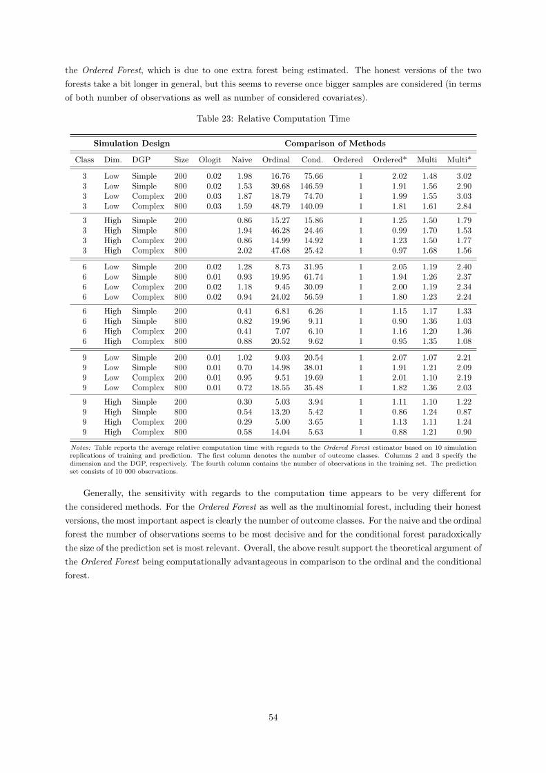
the Ordered Forest, which is due to one extra forest being estimated. The honest versions of the two
forests take a bit longer in general, but this seems to reverse once bigger samples are considered (in terms
of both number of observations as well as number of considered covariates).
Table 23: Relative Computation Time
Simulation Design Comparison of Methods
Class Dim. DGP Size Ologit Naive Ordinal Cond. Ordered Ordered* Multi Multi*
3 Low Simple 200 0.02 1.98 16.76 75.66 1 2.02 1.48 3.023 Low Simple 800 0.02 1.53 39.68 146.59 1 1.91 1.56 2.903 Low Complex 200 0.03 1.87 18.79 74.70 1 1.99 1.55 3.033 Low Complex 800 0.03 1.59 48.79 140.09 1 1.81 1.61 2.84
3 High Simple 200 0.86 15.27 15.86 1 1.25 1.50 1.793 High Simple 800 1.94 46.28 24.46 1 0.99 1.70 1.533 High Complex 200 0.86 14.99 14.92 1 1.23 1.50 1.773 High Complex 800 2.02 47.68 25.42 1 0.97 1.68 1.56
6 Low Simple 200 0.02 1.28 8.73 31.95 1 2.05 1.19 2.406 Low Simple 800 0.01 0.93 19.95 61.74 1 1.94 1.26 2.376 Low Complex 200 0.02 1.18 9.45 30.09 1 2.00 1.19 2.346 Low Complex 800 0.02 0.94 24.02 56.59 1 1.80 1.23 2.24
6 High Simple 200 0.41 6.81 6.26 1 1.15 1.17 1.336 High Simple 800 0.82 19.96 9.11 1 0.90 1.36 1.036 High Complex 200 0.41 7.07 6.10 1 1.16 1.20 1.366 High Complex 800 0.88 20.52 9.62 1 0.95 1.35 1.08
9 Low Simple 200 0.01 1.02 9.03 20.54 1 2.07 1.07 2.219 Low Simple 800 0.01 0.70 14.98 38.01 1 1.91 1.21 2.099 Low Complex 200 0.01 0.95 9.51 19.69 1 2.01 1.10 2.199 Low Complex 800 0.01 0.72 18.55 35.48 1 1.82 1.36 2.03
9 High Simple 200 0.30 5.03 3.94 1 1.11 1.10 1.229 High Simple 800 0.54 13.20 5.42 1 0.86 1.24 0.879 High Complex 200 0.29 5.00 3.65 1 1.13 1.11 1.249 High Complex 800 0.58 14.04 5.63 1 0.88 1.21 0.90
Notes: Table reports the average relative computation time with regards to the Ordered Forest estimator based on 10 simulationreplications of training and prediction. The first column denotes the number of outcome classes. Columns 2 and 3 specify thedimension and the DGP, respectively. The fourth column contains the number of observations in the training set. The predictionset consists of 10 000 observations.
Generally, the sensitivity with regards to the computation time appears to be very different for
the considered methods. For the Ordered Forest as well as the multinomial forest, including their honest
versions, the most important aspect is clearly the number of outcome classes. For the naive and the ordinal
forest the number of observations seems to be most decisive and for the conditional forest paradoxically
the size of the prediction set is most relevant. Overall, the above result support the theoretical argument of
the Ordered Forest being computationally advantageous in comparison to the ordinal and the conditional
forest.
54
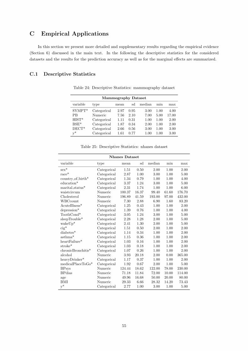
C Empirical Applications
In this section we present more detailed and supplementary results regarding the empirical evidence
(Section 6) discussed in the main text. In the following the descriptive statistics for the considered
datasets and the results for the prediction accuracy as well as for the marginal effects are summarized.
C.1 Descriptive Statistics
Table 24: Descriptive Statistics: mammography dataset
Mammography Dataset
variable type mean sd median min max
SYMPT* Categorical 2.97 0.95 3.00 1.00 4.00PB Numeric 7.56 2.10 7.00 5.00 17.00HIST* Categorical 1.11 0.31 1.00 1.00 2.00BSE* Categorical 1.87 0.34 2.00 1.00 2.00DECT* Categorical 2.66 0.56 3.00 1.00 3.00y* Categorical 1.61 0.77 1.00 1.00 3.00
Table 25: Descriptive Statistics: nhanes dataset
Nhanes Dataset
variable type mean sd median min max
sex* Categorical 1.51 0.50 2.00 1.00 2.00race* Categorical 2.87 1.00 3.00 1.00 5.00country of birth* Categorical 1.34 0.79 1.00 1.00 4.00education* Categorical 3.37 1.24 3.00 1.00 5.00marital status* Categorical 2.31 1.74 1.00 1.00 6.00waistcircum Numeric 100.37 16.37 99.40 61.60 176.70Cholesterol Numeric 196.89 41.59 193.00 97.00 432.00WBCcount Numeric 7.30 2.88 6.90 1.60 83.20AcuteIllness* Categorical 1.25 0.43 1.00 1.00 2.00depression* Categorical 1.39 0.76 1.00 1.00 4.00ToothCond* Categorical 3.05 1.24 3.00 1.00 5.00sleepTrouble* Categorical 2.28 1.28 2.00 1.00 5.00wakeUp* Categorical 2.41 1.30 2.00 1.00 5.00cig* Categorical 1.51 0.50 2.00 1.00 2.00diabetes* Categorical 1.14 0.34 1.00 1.00 2.00asthma* Categorical 1.15 0.36 1.00 1.00 2.00heartFailure* Categorical 1.03 0.16 1.00 1.00 2.00stroke* Categorical 1.03 0.18 1.00 1.00 2.00chronicBronchitis* Categorical 1.07 0.26 1.00 1.00 2.00alcohol Numeric 3.93 20.18 2.00 0.00 365.00heavyDrinker* Categorical 1.17 0.37 1.00 1.00 2.00medicalPlaceToGo* Categorical 1.92 0.67 2.00 1.00 5.00BPsys Numeric 124.44 18.62 122.00 78.00 230.00BPdias Numeric 71.18 11.84 72.00 10.00 114.00age Numeric 49.96 16.68 50.00 20.00 80.00BMI Numeric 29.33 6.66 28.32 14.20 73.43y* Categorical 2.77 1.00 3.00 1.00 5.00
55
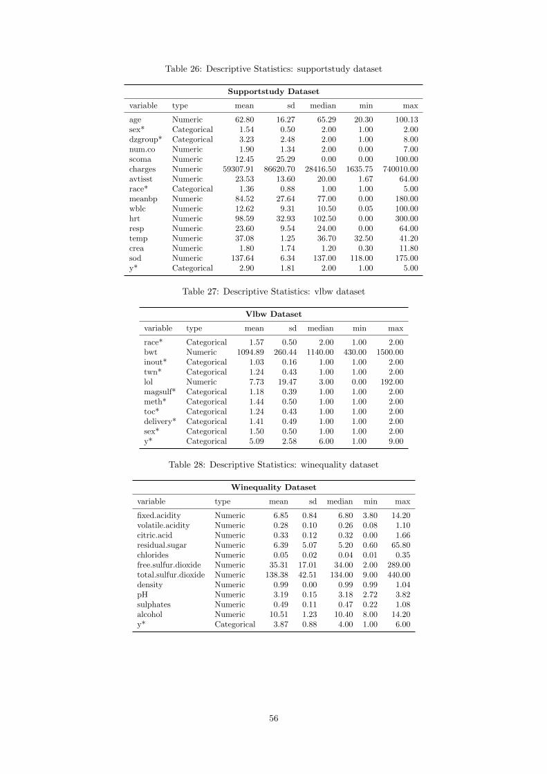
Table 26: Descriptive Statistics: supportstudy dataset
Supportstudy Dataset
variable type mean sd median min max
age Numeric 62.80 16.27 65.29 20.30 100.13sex* Categorical 1.54 0.50 2.00 1.00 2.00dzgroup* Categorical 3.23 2.48 2.00 1.00 8.00num.co Numeric 1.90 1.34 2.00 0.00 7.00scoma Numeric 12.45 25.29 0.00 0.00 100.00charges Numeric 59307.91 86620.70 28416.50 1635.75 740010.00avtisst Numeric 23.53 13.60 20.00 1.67 64.00race* Categorical 1.36 0.88 1.00 1.00 5.00meanbp Numeric 84.52 27.64 77.00 0.00 180.00wblc Numeric 12.62 9.31 10.50 0.05 100.00hrt Numeric 98.59 32.93 102.50 0.00 300.00resp Numeric 23.60 9.54 24.00 0.00 64.00temp Numeric 37.08 1.25 36.70 32.50 41.20crea Numeric 1.80 1.74 1.20 0.30 11.80sod Numeric 137.64 6.34 137.00 118.00 175.00y* Categorical 2.90 1.81 2.00 1.00 5.00
Table 27: Descriptive Statistics: vlbw dataset
Vlbw Dataset
variable type mean sd median min max
race* Categorical 1.57 0.50 2.00 1.00 2.00bwt Numeric 1094.89 260.44 1140.00 430.00 1500.00inout* Categorical 1.03 0.16 1.00 1.00 2.00twn* Categorical 1.24 0.43 1.00 1.00 2.00lol Numeric 7.73 19.47 3.00 0.00 192.00magsulf* Categorical 1.18 0.39 1.00 1.00 2.00meth* Categorical 1.44 0.50 1.00 1.00 2.00toc* Categorical 1.24 0.43 1.00 1.00 2.00delivery* Categorical 1.41 0.49 1.00 1.00 2.00sex* Categorical 1.50 0.50 1.00 1.00 2.00y* Categorical 5.09 2.58 6.00 1.00 9.00
Table 28: Descriptive Statistics: winequality dataset
Winequality Dataset
variable type mean sd median min max
fixed.acidity Numeric 6.85 0.84 6.80 3.80 14.20volatile.acidity Numeric 0.28 0.10 0.26 0.08 1.10citric.acid Numeric 0.33 0.12 0.32 0.00 1.66residual.sugar Numeric 6.39 5.07 5.20 0.60 65.80chlorides Numeric 0.05 0.02 0.04 0.01 0.35free.sulfur.dioxide Numeric 35.31 17.01 34.00 2.00 289.00total.sulfur.dioxide Numeric 138.38 42.51 134.00 9.00 440.00density Numeric 0.99 0.00 0.99 0.99 1.04pH Numeric 3.19 0.15 3.18 2.72 3.82sulphates Numeric 0.49 0.11 0.47 0.22 1.08alcohol Numeric 10.51 1.23 10.40 8.00 14.20y* Categorical 3.87 0.88 4.00 1.00 6.00
56
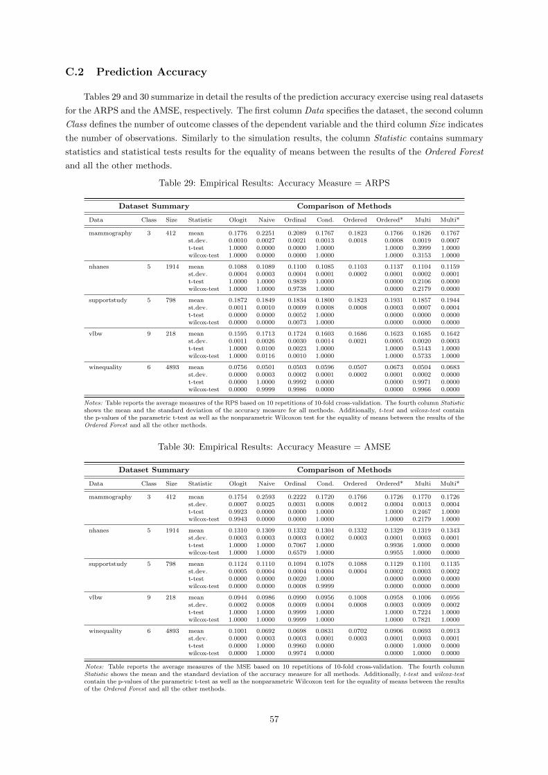
C.2 Prediction Accuracy
Tables 29 and 30 summarize in detail the results of the prediction accuracy exercise using real datasets
for the ARPS and the AMSE, respectively. The first column Data specifies the dataset, the second column
Class defines the number of outcome classes of the dependent variable and the third column Size indicates
the number of observations. Similarly to the simulation results, the column Statistic contains summary
statistics and statistical tests results for the equality of means between the results of the Ordered Forest
and all the other methods.
Table 29: Empirical Results: Accuracy Measure = ARPS
Dataset Summary Comparison of Methods
Data Class Size Statistic Ologit Naive Ordinal Cond. Ordered Ordered* Multi Multi*
mammography 3 412 mean 0.1776 0.2251 0.2089 0.1767 0.1823 0.1766 0.1826 0.1767st.dev. 0.0010 0.0027 0.0021 0.0013 0.0018 0.0008 0.0019 0.0007t-test 1.0000 0.0000 0.0000 1.0000 1.0000 0.3999 1.0000wilcox-test 1.0000 0.0000 0.0000 1.0000 1.0000 0.3153 1.0000
nhanes 5 1914 mean 0.1088 0.1089 0.1100 0.1085 0.1103 0.1137 0.1104 0.1159st.dev. 0.0004 0.0003 0.0004 0.0001 0.0002 0.0001 0.0002 0.0001t-test 1.0000 1.0000 0.9839 1.0000 0.0000 0.2106 0.0000wilcox-test 1.0000 1.0000 0.9738 1.0000 0.0000 0.2179 0.0000
supportstudy 5 798 mean 0.1872 0.1849 0.1834 0.1800 0.1823 0.1931 0.1857 0.1944st.dev. 0.0011 0.0010 0.0009 0.0008 0.0008 0.0003 0.0007 0.0004t-test 0.0000 0.0000 0.0052 1.0000 0.0000 0.0000 0.0000wilcox-test 0.0000 0.0000 0.0073 1.0000 0.0000 0.0000 0.0000
vlbw 9 218 mean 0.1595 0.1713 0.1724 0.1603 0.1686 0.1623 0.1685 0.1642st.dev. 0.0011 0.0026 0.0030 0.0014 0.0021 0.0005 0.0020 0.0003t-test 1.0000 0.0100 0.0023 1.0000 1.0000 0.5143 1.0000wilcox-test 1.0000 0.0116 0.0010 1.0000 1.0000 0.5733 1.0000
winequality 6 4893 mean 0.0756 0.0501 0.0503 0.0596 0.0507 0.0673 0.0504 0.0683st.dev. 0.0000 0.0003 0.0002 0.0001 0.0002 0.0001 0.0002 0.0000t-test 0.0000 1.0000 0.9992 0.0000 0.0000 0.9971 0.0000wilcox-test 0.0000 0.9999 0.9986 0.0000 0.0000 0.9966 0.0000
Notes: Table reports the average measures of the RPS based on 10 repetitions of 10-fold cross-validation. The fourth column Statisticshows the mean and the standard deviation of the accuracy measure for all methods. Additionally, t-test and wilcox-test containthe p-values of the parametric t-test as well as the nonparametric Wilcoxon test for the equality of means between the results of theOrdered Forest and all the other methods.
Table 30: Empirical Results: Accuracy Measure = AMSE
Dataset Summary Comparison of Methods
Data Class Size Statistic Ologit Naive Ordinal Cond. Ordered Ordered* Multi Multi*
mammography 3 412 mean 0.1754 0.2593 0.2222 0.1720 0.1766 0.1726 0.1770 0.1726st.dev. 0.0007 0.0025 0.0031 0.0008 0.0012 0.0004 0.0013 0.0004t-test 0.9923 0.0000 0.0000 1.0000 1.0000 0.2467 1.0000wilcox-test 0.9943 0.0000 0.0000 1.0000 1.0000 0.2179 1.0000
nhanes 5 1914 mean 0.1310 0.1309 0.1332 0.1304 0.1332 0.1329 0.1319 0.1343st.dev. 0.0003 0.0003 0.0003 0.0002 0.0003 0.0001 0.0003 0.0001t-test 1.0000 1.0000 0.7067 1.0000 0.9936 1.0000 0.0000wilcox-test 1.0000 1.0000 0.6579 1.0000 0.9955 1.0000 0.0000
supportstudy 5 798 mean 0.1124 0.1110 0.1094 0.1078 0.1088 0.1129 0.1101 0.1135st.dev. 0.0005 0.0004 0.0004 0.0004 0.0004 0.0002 0.0003 0.0002t-test 0.0000 0.0000 0.0020 1.0000 0.0000 0.0000 0.0000wilcox-test 0.0000 0.0000 0.0008 0.9999 0.0000 0.0000 0.0000
vlbw 9 218 mean 0.0944 0.0986 0.0990 0.0956 0.1008 0.0958 0.1006 0.0956st.dev. 0.0002 0.0008 0.0009 0.0004 0.0008 0.0003 0.0009 0.0002t-test 1.0000 1.0000 0.9999 1.0000 1.0000 0.7224 1.0000wilcox-test 1.0000 1.0000 0.9999 1.0000 1.0000 0.7821 1.0000
winequality 6 4893 mean 0.1001 0.0692 0.0698 0.0831 0.0702 0.0906 0.0693 0.0913st.dev. 0.0000 0.0003 0.0003 0.0001 0.0003 0.0001 0.0003 0.0001t-test 0.0000 1.0000 0.9960 0.0000 0.0000 1.0000 0.0000wilcox-test 0.0000 1.0000 0.9974 0.0000 0.0000 1.0000 0.0000
Notes: Table reports the average measures of the MSE based on 10 repetitions of 10-fold cross-validation. The fourth columnStatistic shows the mean and the standard deviation of the accuracy measure for all methods. Additionally, t-test and wilcox-testcontain the p-values of the parametric t-test as well as the nonparametric Wilcoxon test for the equality of means between the resultsof the Ordered Forest and all the other methods.
57

C.3 Marginal Effects
In what follows, the results for the marginal effects at mean and the mean marginal effects are
presented for all considered datasets. Similarly as in the main text, the effects are computed for each
outcome class of the dependent variable both for the Ordered Forest as well as for the ordered logit.
C.3.1 Data: mammography
Table 31: Marginal Effects at Mean: Mammography Dataset
Dataset Ordered Forest Ordered Logit
Variable Class Effect Std.Error t-Value p-Value Effect Std.Error t-Value p-Value
BSE 1 -0.2965 0.2199 -1.3481 0.1776 -0.2558 0.0912 -2.8056 0.0050 ***2 0.1844 0.1131 1.6307 0.1030 0.1277 0.0486 2.6257 0.0086 ***3 0.1121 0.1918 0.5845 0.5589 0.1280 0.0456 2.8076 0.0050 ***
DECT 1 -0.1908 0.1932 -0.9874 0.3234 -0.0475 0.0529 -0.8978 0.36932 0.2441 0.1311 1.8623 0.0626 * 0.0237 0.0267 0.8897 0.37373 -0.0533 0.1835 -0.2906 0.7714 0.0238 0.0264 0.8997 0.3683
HIST 1 -0.0854 0.1950 -0.4378 0.6615 -0.1829 0.0712 -2.5690 0.0102 **2 0.0602 0.1914 0.3143 0.7533 0.0914 0.0374 2.4459 0.0144 **3 0.0252 0.2662 0.0948 0.9245 0.0916 0.0359 2.5507 0.0108 **
PB 1 0.0180 0.1451 0.1243 0.9011 0.0345 0.0133 2.6056 0.0092 ***2 -0.0990 0.1182 -0.8376 0.4023 -0.0172 0.0070 -2.4779 0.0132 **3 0.0810 0.1683 0.4812 0.6304 -0.0173 0.0067 -2.5860 0.0097 ***
SYMPT 1 -0.2633 0.2303 -1.1433 0.2529 -0.1381 0.0300 -4.6085 0.0000 ***2 0.3143 0.1141 2.7541 0.0059 *** 0.0690 0.0173 3.9801 0.0001 ***3 -0.0510 0.1742 -0.2928 0.7697 0.0691 0.0153 4.5242 0.0000 ***
Significance levels correspond to: ∗ ∗ ∗. < 0.01, ∗ ∗ . < 0.05, ∗. < 0.1.
Notes: Table shows the comparison of the marginal effects at the covariates means between the Ordered Forestand the ordered logit. The effects are estimated for all classes, together with the corresponding standarderrors, t-values and p-values. The standard errors for the Ordered Forest are estimated using the weight-basedinference and the standard errors for the ordered logit are obtained via the delta method.
Table 32: Mean Marginal Effects: Mammography Dataset
Dataset Ordered Forest Ordered Logit
Variable Class Effect Std.Error t-Value p-Value Effect Std.Error t-Value p-Value
BSE 1 -0.1523 0.1013 -1.5032 0.1328 -0.2227 0.0776 -2.8699 0.0041 ***2 0.0757 0.0657 1.1511 0.2497 0.0836 0.0296 2.8229 0.0048 ***3 0.0766 0.1064 0.7200 0.4715 0.1391 0.0507 2.7458 0.0060 ***
DECT 1 -0.0825 0.0784 -1.0528 0.2924 -0.0414 0.0460 -0.8995 0.36842 0.1176 0.0534 2.2018 0.0277 ** 0.0155 0.0173 0.8957 0.37043 -0.0351 0.1047 -0.3352 0.7375 0.0258 0.0288 0.8969 0.3698
HIST 1 -0.0872 0.1180 -0.7394 0.4597 -0.1593 0.0609 -2.6154 0.0089 ***2 0.0832 0.1063 0.7831 0.4335 0.0598 0.0242 2.4662 0.0137 **3 0.0040 0.1505 0.0263 0.9790 0.0995 0.0384 2.5914 0.0096 ***
PB 1 0.0204 0.0695 0.2941 0.7687 0.0301 0.0113 2.6714 0.0076 ***2 -0.0382 0.0589 -0.6483 0.5168 -0.0113 0.0044 -2.5935 0.0095 ***3 0.0177 0.0745 0.2380 0.8119 -0.0188 0.0072 -2.5936 0.0095 ***
SYMPT 1 -0.2237 0.1255 -1.7816 0.0748 * -0.1202 0.0241 -4.9972 0.0000 ***2 0.2472 0.0513 4.8180 0.0000 *** 0.0451 0.0097 4.6455 0.0000 ***3 -0.0236 0.0939 -0.2510 0.8018 0.0751 0.0168 4.4752 0.0000 ***
Significance levels correspond to: ∗ ∗ ∗. < 0.01, ∗ ∗ . < 0.05, ∗. < 0.1.
Notes: Table shows the comparison of the mean marginal effects between the Ordered Forest and the orderedlogit. The effects are estimated for all classes, together with the corresponding standard errors, t-values andp-values. The standard errors for the Ordered Forest are estimated using the weight-based inference and thestandard errors for the ordered logit are obtained via the delta method.
58

C.3.2 Data: nhanes
Table 33: Marginal Effects at Mean: Nhanes Dataset
Dataset Ordered Forest Ordered Logit
Variable Class Effect Std.Error t-Value p-Value Effect Std.Error t-Value p-Value
Acute 1 -0.0018 0.0034 -0.5200 0.6031 -0.0130 0.0052 -2.5150 0.0119 **
Illness 2 -0.0061 0.0065 -0.9416 0.3464 -0.0417 0.0171 -2.4379 0.0148 **
3 0.0048 0.0075 0.6423 0.5206 0.0198 0.0074 2.6867 0.0072 ***
4 0.0011 0.0069 0.1615 0.8717 0.0303 0.0131 2.3121 0.0208 **
5 0.0019 0.0115 0.1689 0.8659 0.0047 0.0021 2.1963 0.0281 **
age 1 -0.0002 0.0004 -0.5008 0.6165 -0.0004 0.0002 -2.0922 0.0364 **
2 -0.0003 0.0010 -0.3376 0.7356 -0.0012 0.0006 -2.1036 0.0354 **
3 0.0003 0.0009 0.2956 0.7675 0.0007 0.0003 2.0716 0.0383 **
4 0.0002 0.0005 0.4970 0.6192 0.0009 0.0004 2.1011 0.0356 **
5 0.0000 0.0001 0.0683 0.9456 0.0001 0.0001 2.0462 0.0407 **
alcohol 1 0.0009 0.0018 0.4777 0.6329 0.0001 0.0001 0.4906 0.6237
2 -0.0002 0.0046 -0.0344 0.9726 0.0002 0.0004 0.4906 0.6237
3 -0.0007 0.0044 -0.1676 0.8669 -0.0001 0.0002 -0.4902 0.6240
4 0.0001 0.0005 0.1580 0.8745 -0.0001 0.0003 -0.4906 0.6237
5 -0.0001 0.0004 -0.1176 0.9064 -0.0000 0.0000 -0.4901 0.6241
asthma 1 -0.0033 0.0016 -1.9998 0.0455 ** -0.0178 0.0059 -3.0366 0.0024 ***
2 -0.0090 0.0087 -1.0383 0.2991 -0.0592 0.0208 -2.8487 0.0044 ***
3 -0.0170 0.0171 -0.9941 0.3202 0.0246 0.0067 3.6693 0.0002 ***
4 0.0275 0.0173 1.5951 0.1107 0.0452 0.0176 2.5661 0.0103 **
5 0.0017 0.0048 0.3599 0.7189 0.0072 0.0030 2.3756 0.0175 **
BMI 1 -0.0019 0.0021 -0.9234 0.3558 -0.0022 0.0009 -2.3115 0.0208 **
2 -0.0075 0.0058 -1.2857 0.1986 -0.0067 0.0029 -2.3256 0.0200 **
3 0.0083 0.0055 1.5210 0.1283 0.0036 0.0016 2.2842 0.0224 **
4 0.0010 0.0008 1.2231 0.2213 0.0046 0.0020 2.3203 0.0203 **
5 0.0001 0.0009 0.0774 0.9383 0.0007 0.0003 2.2570 0.0240 **
BPdias 1 0.0002 0.0004 0.5164 0.6056 0.0003 0.0002 1.4160 0.1568
2 0.0003 0.0019 0.1860 0.8525 0.0010 0.0007 1.4177 0.1563
3 -0.0005 0.0019 -0.2693 0.7877 -0.0005 0.0004 -1.4083 0.1591
4 -0.0000 0.0001 -0.3651 0.7151 -0.0007 0.0005 -1.4175 0.1563
5 -0.0000 0.0001 -0.1235 0.9017 -0.0001 0.0001 -1.3992 0.1618
BPsys 1 -0.0003 0.0001 -2.1923 0.0284 ** -0.0003 0.0002 -1.8747 0.0608 *
2 -0.0004 0.0007 -0.5487 0.5832 -0.0009 0.0005 -1.8820 0.0598 *
3 0.0007 0.0006 1.1788 0.2385 0.0005 0.0003 1.8567 0.0634 *
4 -0.0000 0.0003 -0.1614 0.8718 0.0006 0.0003 1.8814 0.0599 *
5 -0.0000 0.0002 -0.1657 0.8684 0.0001 0.0001 1.8484 0.0645 *
Cholesterol 1 -0.0001 0.0001 -1.0401 0.2983 -0.0001 0.0001 -1.8212 0.0686 *
2 -0.0003 0.0006 -0.5020 0.6157 -0.0003 0.0002 -1.8276 0.0676 *
3 0.0004 0.0005 0.7864 0.4317 0.0002 0.0001 1.8068 0.0708 *
4 0.0000 0.0003 0.0349 0.9722 0.0002 0.0001 1.8253 0.0680 *
5 0.0000 0.0000 0.0122 0.9903 0.0000 0.0000 1.7956 0.0726 *
chronic 1 -0.0016 0.0008 -2.0669 0.0387 ** -0.0155 0.0078 -1.9844 0.0472 **
Bronchitis 2 -0.0255 0.0147 -1.7405 0.0818 * -0.0519 0.0282 -1.8362 0.0663 *
3 0.0101 0.0213 0.4727 0.6364 0.0212 0.0082 2.5786 0.0099 ***
4 0.0119 0.0227 0.5235 0.6006 0.0398 0.0242 1.6470 0.0995 *
5 0.0052 0.0088 0.5871 0.5571 0.0063 0.0041 1.5517 0.1207
cig 1 -0.0080 0.0023 -3.5146 0.0004 *** -0.0006 0.0052 -0.1226 0.9024
2 -0.0078 0.0092 -0.8403 0.4007 -0.0020 0.0160 -0.1226 0.9024
3 0.0160 0.0078 2.0405 0.0413 ** 0.0010 0.0085 0.1226 0.9024
4 -0.0003 0.0040 -0.0838 0.9333 0.0014 0.0110 0.1227 0.9024
Continued on next page
59

Variable Class Effect Std.Error t-Value p-Value Effect Std.Error t-Value p-Value
5 0.0001 0.0005 0.2873 0.7739 0.0002 0.0017 0.1226 0.9024
country 1 0.0004 0.0014 0.2836 0.7767 -0.0058 0.0023 -2.4975 0.0125 **
of birth 2 -0.0383 0.0101 -3.7986 0.0001 *** -0.0177 0.0070 -2.5150 0.0119 **
3 0.0240 0.0095 2.5330 0.0113 ** 0.0094 0.0038 2.4553 0.0141 **
4 0.0145 0.0073 1.9856 0.0471 ** 0.0122 0.0049 2.5144 0.0119 **
5 -0.0007 0.0026 -0.2677 0.7889 0.0018 0.0008 2.4303 0.0151 **
depression 1 -0.0162 0.0068 -2.3879 0.0169 ** -0.0259 0.0039 -6.5902 0.0000 ***
2 -0.0485 0.0256 -1.8961 0.0579 * -0.0794 0.0112 -7.0622 0.0000 ***
3 -0.0323 0.0460 -0.7014 0.4831 0.0422 0.0069 6.1140 0.0000 ***
4 0.0879 0.0510 1.7219 0.0851 * 0.0549 0.0080 6.8425 0.0000 ***
5 0.0091 0.0080 1.1391 0.2547 0.0083 0.0015 5.6826 0.0000 ***
diabetes 1 -0.0065 0.0014 -4.6666 0.0000 *** -0.0360 0.0053 -6.8105 0.0000 ***
2 -0.0924 0.0237 -3.8952 0.0001 *** -0.1306 0.0198 -6.6046 0.0000 ***
3 0.0168 0.0344 0.4892 0.6247 0.0304 0.0074 4.0835 0.0000 ***
4 0.0737 0.0306 2.4114 0.0159 ** 0.1160 0.0228 5.0847 0.0000 ***
5 0.0083 0.0180 0.4598 0.6457 0.0202 0.0049 4.1153 0.0000 ***
education 1 0.0052 0.0020 2.5685 0.0102 ** 0.0212 0.0025 8.3573 0.0000 ***
2 0.0869 0.0424 2.0509 0.0403 ** 0.0649 0.0072 9.0756 0.0000 ***
3 -0.0685 0.0333 -2.0552 0.0399 ** -0.0345 0.0048 -7.2061 0.0000 ***
4 -0.0231 0.0183 -1.2651 0.2058 -0.0448 0.0050 -8.8831 0.0000 ***
5 -0.0004 0.0012 -0.3236 0.7463 -0.0068 0.0010 -6.5114 0.0000 ***
heart 1 0.0000 0.0000 0.0000 1.0000 -0.0288 0.0091 -3.1696 0.0015 ***
Failure 2 -0.0168 0.0073 -2.3092 0.0209 ** -0.1068 0.0395 -2.7007 0.0069 ***
3 -0.0266 0.0607 -0.4388 0.6608 0.0228 0.0094 2.4225 0.0154 **
4 0.0369 0.0481 0.7683 0.4423 0.0960 0.0466 2.0618 0.0392 **
5 0.0065 0.0719 0.0903 0.9280 0.0167 0.0095 1.7645 0.0777 *
heavy 1 -0.0057 0.0024 -2.3815 0.0172 ** -0.0127 0.0061 -2.0982 0.0359 **
Drinker 2 -0.0221 0.0092 -2.4012 0.0163 ** -0.0413 0.0207 -2.0010 0.0454 **
3 0.0224 0.0088 2.5528 0.0107 ** 0.0189 0.0081 2.3399 0.0193 **
4 0.0032 0.0060 0.5317 0.5949 0.0305 0.0163 1.8718 0.0612 *
5 0.0023 0.0100 0.2296 0.8184 0.0047 0.0027 1.7838 0.0745 *
marital 1 -0.0007 0.0007 -0.9425 0.3459 -0.0025 0.0015 -1.6584 0.0972 *
status 2 -0.0016 0.0041 -0.3818 0.7026 -0.0076 0.0045 -1.6631 0.0963 *
3 0.0027 0.0037 0.7438 0.4570 0.0040 0.0024 1.6471 0.0995 *
4 -0.0005 0.0026 -0.1987 0.8425 0.0052 0.0031 1.6618 0.0965 *
5 0.0000 0.0002 0.1985 0.8426 0.0008 0.0005 1.6375 0.1015
medical 1 -0.0004 0.0019 -0.2220 0.8243 0.0003 0.0036 0.0728 0.9420
Place 2 0.0049 0.0089 0.5515 0.5813 0.0008 0.0111 0.0728 0.9420
To Go 3 -0.0033 0.0073 -0.4562 0.6483 -0.0004 0.0059 -0.0728 0.9420
4 -0.0008 0.0037 -0.2087 0.8347 -0.0006 0.0077 -0.0728 0.9420
5 -0.0004 0.0025 -0.1591 0.8736 -0.0001 0.0012 -0.0728 0.9420
race 1 0.0043 0.0014 3.0319 0.0024 *** 0.0050 0.0026 1.9649 0.0494 **
2 0.0172 0.0094 1.8371 0.0662 * 0.0154 0.0078 1.9785 0.0479 **
3 -0.0196 0.0086 -2.2729 0.0230 ** -0.0082 0.0042 -1.9422 0.0521 *
4 -0.0025 0.0059 -0.4262 0.6700 -0.0106 0.0054 -1.9803 0.0477 **
5 0.0005 0.0025 0.2158 0.8292 -0.0016 0.0008 -1.9426 0.0521 *
sex 1 0.0075 0.0059 1.2739 0.2027 0.0096 0.0059 1.6327 0.1025
2 -0.0153 0.0098 -1.5559 0.1197 0.0294 0.0179 1.6455 0.0999 *
3 0.0082 0.0089 0.9128 0.3613 -0.0156 0.0096 -1.6286 0.1034
4 -0.0002 0.0019 -0.1288 0.8975 -0.0203 0.0124 -1.6424 0.1005
5 -0.0001 0.0006 -0.1969 0.8439 -0.0031 0.0019 -1.6152 0.1063
sleep 1 -0.0037 0.0017 -2.2193 0.0265 ** -0.0021 0.0024 -0.8571 0.3914
Trouble 2 -0.0141 0.0125 -1.1235 0.2612 -0.0063 0.0073 -0.8575 0.3912
3 0.0109 0.0107 1.0153 0.3100 0.0033 0.0039 0.8556 0.3922
4 0.0069 0.0122 0.5625 0.5737 0.0043 0.0051 0.8574 0.3912
Continued on next page
60

Variable Class Effect Std.Error t-Value p-Value Effect Std.Error t-Value p-Value
5 0.0000 0.0004 0.1169 0.9070 0.0007 0.0008 0.8529 0.3937
stroke 1 0.0000 0.0000 0.0000 1.0000 -0.0312 0.0075 -4.1883 0.0000 ***
2 -0.0333 0.0094 -3.5432 0.0004 *** -0.1175 0.0326 -3.6003 0.0003 ***
3 0.0145 0.0189 0.7676 0.4427 0.0209 0.0111 1.8806 0.0600 *
4 -0.0045 0.0228 -0.1951 0.8453 0.1086 0.0405 2.6834 0.0073 ***
5 0.0232 0.0344 0.6746 0.4999 0.0193 0.0086 2.2298 0.0258 **
Tooth 1 -0.0052 0.0021 -2.4413 0.0146 ** -0.0230 0.0025 -9.0333 0.0000 ***
Cond 2 -0.1008 0.0238 -4.2327 0.0000 *** -0.0705 0.0071 -9.9072 0.0000 ***
3 0.0193 0.0488 0.3946 0.6932 0.0374 0.0050 7.5175 0.0000 ***
4 0.0862 0.0551 1.5647 0.1176 0.0487 0.0050 9.8287 0.0000 ***
5 0.0004 0.0024 0.1735 0.8623 0.0074 0.0011 6.7816 0.0000 ***
waist 1 -0.0006 0.0004 -1.4128 0.1577 -0.0006 0.0004 -1.3994 0.1617
circum 2 0.0009 0.0018 0.5026 0.6152 -0.0017 0.0012 -1.4015 0.1611
3 -0.0003 0.0017 -0.1823 0.8553 0.0009 0.0007 1.3900 0.1645
4 0.0000 0.0006 0.0112 0.9911 0.0012 0.0009 1.4026 0.1607
5 0.0000 0.0000 0.0000 1.0000 0.0002 0.0001 1.3859 0.1658
wakeUp 1 -0.0018 0.0018 -1.0045 0.3152 -0.0033 0.0023 -1.4339 0.1516
2 -0.0088 0.0125 -0.7028 0.4822 -0.0102 0.0071 -1.4402 0.1498
3 0.0107 0.0116 0.9237 0.3557 0.0054 0.0038 1.4273 0.1535
4 -0.0002 0.0023 -0.0822 0.9345 0.0071 0.0049 1.4390 0.1501
5 0.0001 0.0004 0.2059 0.8369 0.0011 0.0007 1.4280 0.1533
WBCcount 1 0.0010 0.0022 0.4391 0.6606 0.0009 0.0009 0.9893 0.3225
2 -0.0089 0.0080 -1.1100 0.2670 0.0027 0.0027 0.9900 0.3222
3 0.0038 0.0077 0.4984 0.6182 -0.0014 0.0015 -0.9864 0.3239
4 0.0041 0.0048 0.8583 0.3907 -0.0019 0.0019 -0.9900 0.3222
5 -0.0000 0.0029 -0.0022 0.9983 -0.0003 0.0003 -0.9849 0.3247
Significance levels correspond to: ∗ ∗ ∗. < 0.01, ∗ ∗ . < 0.05, ∗. < 0.1.
Notes: Table shows the comparison of the marginal effects at the covariates means between the Ordered Forest
and the ordered logit. The effects are estimated for all classes, together with the corresponding standard errors,
t-values and p-values. The standard errors for the Ordered Forest are estimated using the weight-based inference
and the standard errors for the ordered logit are obtained via the delta method.
61

Table 34: Mean Marginal Effects: Nhanes Dataset
Dataset Ordered Forest Ordered Logit
Variable Class Effect Std.Error t-Value p-Value Effect Std.Error t-Value p-Value
Acute 1 -0.0035 0.0020 -1.7500 0.0801 * -0.0192 0.0076 -2.5131 0.0120 **
Illness 2 -0.0036 0.0036 -0.9918 0.3213 -0.0253 0.0108 -2.3431 0.0191 **
3 0.0012 0.0047 0.2525 0.8007 0.0119 0.0046 2.6025 0.0093 ***
4 0.0022 0.0062 0.3585 0.7199 0.0237 0.0101 2.3507 0.0187 **
5 0.0037 0.0109 0.3407 0.7333 0.0090 0.0039 2.2896 0.0220 **
age 1 -0.0007 0.0002 -3.2796 0.0010 *** -0.0006 0.0003 -2.0982 0.0359 **
2 0.0002 0.0004 0.5748 0.5654 -0.0007 0.0003 -2.1099 0.0349 **
3 -0.0001 0.0004 -0.3504 0.7261 0.0004 0.0002 2.1012 0.0356 **
4 0.0006 0.0002 2.4133 0.0158 ** 0.0007 0.0003 2.1053 0.0353 **
5 0.0000 0.0001 0.3204 0.7486 0.0003 0.0001 2.0708 0.0384 **
alcohol 1 0.0011 0.0009 1.1316 0.2578 0.0001 0.0002 0.4907 0.6236
2 0.0020 0.0021 0.9193 0.3579 0.0001 0.0002 0.4906 0.6237
3 0.0010 0.0020 0.4786 0.6322 -0.0001 0.0001 -0.4906 0.6237
4 -0.0033 0.0017 -1.9123 0.0558 * -0.0001 0.0002 -0.4907 0.6237
5 -0.0007 0.0010 -0.6934 0.4881 -0.0000 0.0001 -0.4903 0.6239
asthma 1 -0.0025 0.0011 -2.2316 0.0256 ** -0.0266 0.0089 -3.0008 0.0027 ***
2 -0.0022 0.0039 -0.5566 0.5778 -0.0368 0.0137 -2.6758 0.0075 ***
3 -0.0050 0.0090 -0.5638 0.5729 0.0153 0.0045 3.4041 0.0007 ***
4 0.0063 0.0075 0.8415 0.4001 0.0344 0.0129 2.6660 0.0077 ***
5 0.0034 0.0051 0.6653 0.5059 0.0135 0.0054 2.5135 0.0120 **
BMI 1 -0.0016 0.0006 -2.5492 0.0108 ** -0.0032 0.0014 -2.3182 0.0204 **
2 -0.0030 0.0010 -3.1102 0.0019 *** -0.0039 0.0017 -2.3278 0.0199 **
3 0.0030 0.0009 3.1571 0.0016 *** 0.0021 0.0009 2.2983 0.0215 **
4 0.0012 0.0006 1.9253 0.0542 * 0.0037 0.0016 2.3333 0.0196 **
5 0.0003 0.0006 0.4878 0.6257 0.0014 0.0006 2.2857 0.0223 **
BPdias 1 -0.0002 0.0002 -1.2828 0.1996 0.0005 0.0003 1.4176 0.1563
2 0.0008 0.0004 2.0067 0.0448 ** 0.0006 0.0004 1.4184 0.1561
3 -0.0002 0.0004 -0.6035 0.5462 -0.0003 0.0002 -1.4178 0.1562
4 -0.0003 0.0003 -1.0130 0.3111 -0.0005 0.0004 -1.4173 0.1564
5 -0.0000 0.0002 -0.0291 0.9768 -0.0002 0.0001 -1.4087 0.1589
BPsys 1 -0.0001 0.0002 -0.6735 0.5006 -0.0004 0.0002 -1.8801 0.0601 *
2 -0.0002 0.0002 -0.7668 0.4432 -0.0005 0.0003 -1.8825 0.0598 *
3 0.0001 0.0002 0.6724 0.5013 0.0003 0.0002 1.8691 0.0616 *
4 0.0002 0.0001 1.1666 0.2434 0.0005 0.0003 1.8840 0.0596 *
5 -0.0000 0.0001 -0.0913 0.9273 0.0002 0.0001 1.8662 0.0620 *
Cholesterol 1 -0.0001 0.0000 -1.9336 0.0532 * -0.0002 0.0001 -1.8253 0.0680 *
2 0.0000 0.0001 0.3347 0.7379 -0.0002 0.0001 -1.8281 0.0675 *
3 0.0001 0.0001 0.7192 0.4720 0.0001 0.0001 1.8160 0.0694 *
4 -0.0000 0.0001 -0.0785 0.9374 0.0002 0.0001 1.8302 0.0672 *
5 -0.0000 0.0000 -0.0415 0.9669 0.0001 0.0000 1.8098 0.0703 *
chronic 1 -0.0013 0.0009 -1.4752 0.1402 -0.0231 0.0119 -1.9495 0.0512 *
Bronchitis 2 -0.0124 0.0068 -1.8302 0.0672 * -0.0324 0.0189 -1.7128 0.0867 *
3 -0.0067 0.0106 -0.6315 0.5277 0.0133 0.0059 2.2572 0.0240 **
4 0.0155 0.0093 1.6701 0.0949 * 0.0303 0.0177 1.7123 0.0868 *
5 0.0049 0.0079 0.6221 0.5339 0.0119 0.0073 1.6294 0.1032
cig 1 -0.0042 0.0016 -2.6060 0.0092 *** -0.0009 0.0076 -0.1227 0.9024
2 -0.0015 0.0032 -0.4697 0.6386 -0.0011 0.0093 -0.1225 0.9025
3 0.0054 0.0028 1.9314 0.0534 * 0.0006 0.0049 0.1225 0.9025
4 0.0000 0.0022 0.0198 0.9842 0.0011 0.0088 0.1226 0.9024
5 0.0003 0.0010 0.2799 0.7795 0.0004 0.0033 0.1227 0.9023
country 1 -0.0004 0.0007 -0.5361 0.5919 -0.0084 0.0034 -2.5107 0.0120 **
of birth 2 -0.0197 0.0046 -4.3165 0.0000 *** -0.0103 0.0041 -2.5124 0.0120 **
Continued on next page
62

Variable Class Effect Std.Error t-Value p-Value Effect Std.Error t-Value p-Value
3 0.0117 0.0046 2.5288 0.0114 ** 0.0054 0.0022 2.4810 0.0131 **
4 0.0090 0.0038 2.3771 0.0175 ** 0.0097 0.0038 2.5190 0.0118 **
5 -0.0006 0.0024 -0.2627 0.7928 0.0037 0.0015 2.4750 0.0133 **
depression 1 -0.0163 0.0053 -3.0802 0.0021 *** -0.0379 0.0056 -6.7712 0.0000 ***
2 -0.0557 0.0158 -3.5277 0.0004 *** -0.0463 0.0066 -7.0602 0.0000 ***
3 -0.0171 0.0240 -0.7116 0.4767 0.0244 0.0039 6.1918 0.0000 ***
4 0.0768 0.0259 2.9620 0.0031 *** 0.0435 0.0060 7.2491 0.0000 ***
5 0.0122 0.0076 1.6171 0.1059 0.0164 0.0026 6.2019 0.0000 ***
diabetes 1 -0.0045 0.0008 -5.6471 0.0000 *** -0.0534 0.0075 -7.1385 0.0000 ***
2 -0.0719 0.0128 -5.6178 0.0000 *** -0.0914 0.0163 -5.5945 0.0000 ***
3 -0.0039 0.0204 -0.1924 0.8475 0.0235 0.0035 6.8145 0.0000 ***
4 0.0704 0.0152 4.6159 0.0000 *** 0.0867 0.0162 5.3684 0.0000 ***
5 0.0100 0.0162 0.6167 0.5374 0.0346 0.0073 4.7343 0.0000 ***
education 1 0.0034 0.0021 1.6707 0.0948 * 0.0310 0.0036 8.6650 0.0000 ***
2 0.0683 0.0196 3.4769 0.0005 *** 0.0378 0.0039 9.5840 0.0000 ***
3 -0.0460 0.0147 -3.1215 0.0018 *** -0.0199 0.0023 -8.6028 0.0000 ***
4 -0.0254 0.0119 -2.1431 0.0321 ** -0.0355 0.0039 -9.2023 0.0000 ***
5 -0.0003 0.0013 -0.2455 0.8061 -0.0134 0.0018 -7.3984 0.0000 ***
heart 1 -0.0001 0.0000 -6.1333 0.0000 *** -0.0445 0.0147 -3.0275 0.0025 ***
Failure 2 -0.0094 0.0084 -1.1165 0.2642 -0.0723 0.0312 -2.3205 0.0203 **
3 -0.0140 0.0327 -0.4276 0.6689 0.0189 0.0027 6.9672 0.0000 ***
4 0.0262 0.0498 0.5267 0.5984 0.0681 0.0300 2.2698 0.0232 **
5 -0.0027 0.0702 -0.0389 0.9690 0.0298 0.0153 1.9417 0.0522 *
heavy 1 -0.0011 0.0012 -0.9120 0.3618 -0.0188 0.0090 -2.0846 0.0371 **
Drinker 2 -0.0117 0.0045 -2.5987 0.0094 *** -0.0254 0.0133 -1.9027 0.0571 *
3 0.0049 0.0051 0.9683 0.3329 0.0116 0.0053 2.1921 0.0284 **
4 0.0051 0.0055 0.9330 0.3508 0.0236 0.0123 1.9163 0.0553 *
5 0.0027 0.0096 0.2867 0.7744 0.0091 0.0049 1.8575 0.0632 *
marital 1 -0.0006 0.0008 -0.7842 0.4329 -0.0036 0.0022 -1.6598 0.0969 *
status 2 -0.0009 0.0014 -0.6838 0.4941 -0.0044 0.0026 -1.6667 0.0956 *
3 0.0011 0.0013 0.8657 0.3867 0.0023 0.0014 1.6587 0.0972 *
4 0.0004 0.0013 0.3151 0.7527 0.0041 0.0025 1.6651 0.0959 *
5 0.0000 0.0005 0.0106 0.9916 0.0016 0.0009 1.6484 0.0993 *
medical 1 -0.0001 0.0014 -0.0854 0.9319 0.0004 0.0053 0.0728 0.9420
Place 2 0.0037 0.0030 1.2483 0.2119 0.0005 0.0065 0.0728 0.9420
To Go 3 0.0017 0.0031 0.5579 0.5769 -0.0002 0.0034 -0.0728 0.9420
4 -0.0042 0.0020 -2.0705 0.0384 ** -0.0004 0.0061 -0.0728 0.9420
5 -0.0011 0.0024 -0.4592 0.6461 -0.0002 0.0023 -0.0728 0.9420
race 1 0.0027 0.0011 2.5402 0.0111 ** 0.0073 0.0037 1.9699 0.0488 **
2 0.0132 0.0040 3.3347 0.0009 *** 0.0090 0.0045 1.9840 0.0473 **
3 -0.0110 0.0042 -2.6334 0.0085 *** -0.0047 0.0024 -1.9569 0.0504 *
4 -0.0054 0.0032 -1.7011 0.0889 * -0.0084 0.0042 -1.9846 0.0472 **
5 0.0005 0.0027 0.2021 0.8398 -0.0032 0.0016 -1.9595 0.0501 *
sex 1 0.0051 0.0030 1.6862 0.0918 * 0.0140 0.0086 1.6395 0.1011
2 -0.0051 0.0030 -1.6929 0.0905 * 0.0171 0.0104 1.6491 0.0991 *
3 0.0019 0.0023 0.8190 0.4128 -0.0089 0.0054 -1.6515 0.0986 *
4 -0.0010 0.0019 -0.5180 0.6044 -0.0162 0.0099 -1.6388 0.1013
5 -0.0009 0.0019 -0.4967 0.6194 -0.0061 0.0037 -1.6323 0.1026
sleep 1 -0.0017 0.0016 -1.0947 0.2736 -0.0030 0.0035 -0.8574 0.3912
Trouble 2 -0.0018 0.0041 -0.4444 0.6568 -0.0037 0.0043 -0.8583 0.3907
3 -0.0037 0.0056 -0.6554 0.5122 0.0019 0.0022 0.8589 0.3904
4 0.0072 0.0072 1.0120 0.3115 0.0034 0.0040 0.8576 0.3911
5 -0.0000 0.0006 -0.0213 0.9830 0.0013 0.0015 0.8546 0.3928
stroke 1 -0.0000 0.0000 -4.6343 0.0000 *** -0.0484 0.0120 -4.0425 0.0001 ***
2 -0.0199 0.0085 -2.3486 0.0188 ** -0.0810 0.0266 -3.0507 0.0023 ***
3 0.0087 0.0077 1.1393 0.2546 0.0190 0.0031 6.0505 0.0000 ***
Continued on next page
63

Variable Class Effect Std.Error t-Value p-Value Effect Std.Error t-Value p-Value
4 -0.0154 0.0211 -0.7296 0.4656 0.0767 0.0259 2.9564 0.0031 ***
5 0.0265 0.0279 0.9523 0.3409 0.0337 0.0135 2.4900 0.0128 **
Tooth 1 -0.0045 0.0015 -2.9013 0.0037 *** -0.0336 0.0035 -9.5125 0.0000 ***
Cond 2 -0.0609 0.0145 -4.2040 0.0000 *** -0.0411 0.0039 -10.5726 0.0000 ***
3 -0.0303 0.0271 -1.1157 0.2645 0.0216 0.0023 9.3228 0.0000 ***
4 0.0946 0.0327 2.8960 0.0038 *** 0.0386 0.0038 10.1793 0.0000 ***
5 0.0010 0.0023 0.4389 0.6608 0.0145 0.0019 7.8454 0.0000 ***
waist 1 -0.0006 0.0002 -3.1634 0.0016 *** -0.0008 0.0006 -1.4016 0.1610
circum 2 -0.0013 0.0004 -3.3726 0.0007 *** -0.0010 0.0007 -1.4040 0.1603
3 0.0012 0.0004 3.3524 0.0008 *** 0.0005 0.0004 1.4047 0.1601
4 0.0006 0.0003 2.3878 0.0169 ** 0.0009 0.0007 1.4007 0.1613
5 0.0001 0.0002 0.4812 0.6304 0.0004 0.0003 1.3952 0.1630
wakeUp 1 -0.0020 0.0016 -1.2417 0.2143 -0.0049 0.0034 -1.4365 0.1509
2 -0.0025 0.0035 -0.6984 0.4849 -0.0059 0.0041 -1.4398 0.1499
3 0.0028 0.0032 0.8858 0.3757 0.0031 0.0022 1.4280 0.1533
4 0.0016 0.0018 0.8958 0.3703 0.0056 0.0039 1.4407 0.1497
5 0.0000 0.0006 0.0277 0.9779 0.0021 0.0015 1.4353 0.1512
WBCcount 1 -0.0011 0.0009 -1.1499 0.2502 0.0013 0.0013 0.9901 0.3221
2 -0.0023 0.0017 -1.3251 0.1851 0.0016 0.0016 0.9899 0.3222
3 0.0027 0.0015 1.7432 0.0813 * -0.0008 0.0008 -0.9880 0.3231
4 0.0004 0.0011 0.3634 0.7163 -0.0015 0.0015 -0.9904 0.3220
5 0.0003 0.0011 0.2339 0.8151 -0.0006 0.0006 -0.9879 0.3232
Significance levels correspond to: ∗ ∗ ∗. < 0.01, ∗ ∗ . < 0.05, ∗. < 0.1.
Notes: Table shows the comparison of the mean marginal effects between the Ordered Forest and the ordered logit.
The effects are estimated for all classes, together with the corresponding standard errors, t-values and p-values.
The standard errors for the Ordered Forest are estimated using the weight-based inference and the standard errors
for the ordered logit are obtained via the delta method.
64

C.3.3 Data: supportstudy
Table 35: Marginal Effects at Mean: Support Study Dataset
Dataset Ordered Forest Ordered Logit
Variable Class Effect Std.Error t-Value p-Value Effect Std.Error t-Value p-Value
age 1 -0.0008 0.0022 -0.3806 0.7035 -0.0025 0.0011 -2.3050 0.0212 **
2 0.0013 0.0017 0.8107 0.4175 -0.0003 0.0002 -2.0671 0.0387 **
3 -0.0013 0.0019 -0.6882 0.4913 0.0001 0.0001 1.4735 0.1406
4 0.0009 0.0018 0.5167 0.6054 0.0000 0.0000 1.6236 0.1045
5 -0.0001 0.0018 -0.0799 0.9363 0.0027 0.0012 2.3101 0.0209 **
avtisst 1 -0.0036 0.0020 -1.8184 0.0690 * -0.0172 0.0017 -9.8795 0.0000 ***
2 0.0003 0.0017 0.1867 0.8519 -0.0022 0.0006 -3.8999 0.0001 ***
3 0.0023 0.0016 1.4074 0.1593 0.0006 0.0003 1.9432 0.0520 *
4 -0.0004 0.0010 -0.4627 0.6436 0.0002 0.0001 2.2665 0.0234 **
5 0.0015 0.0014 1.0804 0.2800 0.0187 0.0020 9.4419 0.0000 ***
charges 1 -0.0000 0.0000 -1.3547 0.1755 0.0000 0.0000 1.8483 0.0646 *
2 0.0000 0.0000 1.2867 0.1982 0.0000 0.0000 1.6418 0.1006
3 0.0000 0.0000 0.6363 0.5246 -0.0000 0.0000 -1.4242 0.1544
4 0.0000 0.0000 0.7488 0.4540 -0.0000 0.0000 -1.4696 0.1417
5 -0.0000 0.0000 -0.4501 0.6526 -0.0000 0.0000 -1.8310 0.0671 *
crea 1 -0.0305 0.0234 -1.3032 0.1925 -0.0243 0.0103 -2.3478 0.0189 **
2 -0.0172 0.0222 -0.7734 0.4393 -0.0032 0.0016 -2.0295 0.0424 **
3 0.0190 0.0202 0.9370 0.3487 0.0008 0.0005 1.5360 0.1245
4 0.0117 0.0146 0.8000 0.4237 0.0003 0.0002 1.6622 0.0965 *
5 0.0170 0.0273 0.6242 0.5325 0.0264 0.0113 2.3343 0.0196 **
dzgroup 1 -0.0167 0.0100 -1.6654 0.0958 * -0.0453 0.0073 -6.2305 0.0000 ***
2 -0.0550 0.0174 -3.1661 0.0015 *** -0.0059 0.0017 -3.4993 0.0005 ***
3 -0.0115 0.0144 -0.8012 0.4230 0.0016 0.0008 1.8889 0.0589 *
4 -0.0042 0.0086 -0.4937 0.6215 0.0005 0.0002 2.1800 0.0293 **
5 0.0875 0.0293 2.9819 0.0029 *** 0.0491 0.0080 6.1109 0.0000 ***
hrt 1 -0.0002 0.0007 -0.2297 0.8183 -0.0011 0.0006 -1.9711 0.0487 **
2 0.0002 0.0006 0.3185 0.7501 -0.0001 0.0001 -1.8058 0.0710 *
3 -0.0005 0.0010 -0.4462 0.6555 0.0000 0.0000 1.3738 0.1695
4 0.0006 0.0006 1.0007 0.3170 0.0000 0.0000 1.4953 0.1348
5 -0.0002 0.0016 -0.0971 0.9227 0.0012 0.0006 1.9726 0.0485 **
meanbp 1 0.0003 0.0003 0.8334 0.4046 0.0013 0.0006 2.1434 0.0321 **
2 -0.0005 0.0005 -0.9325 0.3511 0.0002 0.0001 1.9143 0.0556 *
3 0.0001 0.0005 0.2744 0.7838 -0.0000 0.0000 -1.4432 0.1490
4 0.0002 0.0003 0.5978 0.5500 -0.0000 0.0000 -1.5715 0.1161
5 -0.0001 0.0004 -0.2825 0.7776 -0.0014 0.0007 -2.1402 0.0323 **
num.co 1 -0.0025 0.0052 -0.4857 0.6272 -0.0024 0.0128 -0.1846 0.8536
2 0.0033 0.0040 0.8202 0.4121 -0.0003 0.0017 -0.1844 0.8537
3 -0.0047 0.0079 -0.5898 0.5553 0.0001 0.0004 0.1838 0.8542
4 0.0031 0.0053 0.5737 0.5661 0.0000 0.0001 0.1840 0.8540
5 0.0008 0.0106 0.0784 0.9375 0.0026 0.0139 0.1846 0.8536
race 1 -0.0095 0.0071 -1.3378 0.1810 -0.0062 0.0183 -0.3400 0.7339
2 0.0068 0.0050 1.3535 0.1759 -0.0008 0.0024 -0.3396 0.7341
3 0.0081 0.0055 1.4697 0.1416 0.0002 0.0006 0.3341 0.7383
4 -0.0045 0.0039 -1.1592 0.2464 0.0001 0.0002 0.3361 0.7368
5 -0.0008 0.0078 -0.1078 0.9141 0.0068 0.0199 0.3401 0.7338
resp 1 0.0010 0.0013 0.7541 0.4508 -0.0060 0.0018 -3.3087 0.0009 ***
2 -0.0002 0.0025 -0.0955 0.9239 -0.0008 0.0003 -2.5951 0.0095 ***
3 -0.0024 0.0027 -0.8679 0.3855 0.0002 0.0001 1.7077 0.0877 *
4 -0.0010 0.0017 -0.6190 0.5359 0.0001 0.0000 1.9037 0.0569 *
Continued on next page
65

Variable Class Effect Std.Error t-Value p-Value Effect Std.Error t-Value p-Value
5 0.0027 0.0017 1.5985 0.1099 0.0065 0.0020 3.2860 0.0010 ***
scoma 1 0.0000 0.0000 0.0000 1.0000 -0.0044 0.0008 -5.3793 0.0000 ***
2 -0.0001 0.0001 -2.0341 0.0419 ** -0.0006 0.0002 -3.2495 0.0012 ***
3 0.0002 0.0001 1.3658 0.1720 0.0002 0.0001 1.8912 0.0586 *
4 -0.0005 0.0001 -3.2260 0.0013 *** 0.0000 0.0000 2.1553 0.0311 **
5 0.0004 0.0001 5.1852 0.0000 *** 0.0048 0.0009 5.2395 0.0000 ***
sex 1 0.0010 0.0077 0.1231 0.9020 -0.0498 0.0326 -1.5286 0.1264
2 0.0048 0.0076 0.6314 0.5278 -0.0065 0.0045 -1.4394 0.1500
3 -0.0077 0.0066 -1.1632 0.2448 0.0017 0.0014 1.2097 0.2264
4 0.0024 0.0056 0.4372 0.6620 0.0005 0.0004 1.2770 0.2016
5 -0.0005 0.0124 -0.0367 0.9708 0.0541 0.0354 1.5271 0.1267
sod 1 0.0026 0.0024 1.0949 0.2735 0.0019 0.0027 0.6870 0.4921
2 -0.0012 0.0019 -0.6318 0.5275 0.0002 0.0004 0.6772 0.4983
3 -0.0006 0.0019 -0.3051 0.7603 -0.0001 0.0001 -0.6504 0.5155
4 0.0005 0.0018 0.2849 0.7757 -0.0000 0.0000 -0.6591 0.5098
5 -0.0014 0.0022 -0.6291 0.5293 -0.0020 0.0030 -0.6867 0.4923
temp 1 0.0044 0.0103 0.4229 0.6724 0.0345 0.0155 2.2297 0.0258 **
2 -0.0016 0.0080 -0.2039 0.8385 0.0045 0.0023 1.9729 0.0485 **
3 -0.0001 0.0063 -0.0225 0.9821 -0.0012 0.0008 -1.4786 0.1392
4 0.0013 0.0056 0.2235 0.8231 -0.0004 0.0002 -1.6114 0.1071
5 -0.0039 0.0051 -0.7534 0.4512 -0.0374 0.0168 -2.2245 0.0261 **
wblc 1 -0.0029 0.0034 -0.8484 0.3962 -0.0007 0.0019 -0.3913 0.6956
2 -0.0019 0.0024 -0.7787 0.4361 -0.0001 0.0003 -0.3892 0.6971
3 0.0010 0.0023 0.4413 0.6590 0.0000 0.0001 0.3840 0.7010
4 0.0023 0.0021 1.0790 0.2806 0.0000 0.0000 0.3858 0.6997
5 0.0015 0.0042 0.3494 0.7268 0.0008 0.0021 0.3912 0.6956
Significance levels correspond to: ∗ ∗ ∗. < 0.01, ∗ ∗ . < 0.05, ∗. < 0.1.
Notes: Table shows the comparison of the marginal effects at the covariates means between the Ordered Forest
and the ordered logit. The effects are estimated for all classes, together with the corresponding standard
errors, t-values and p-values. The standard errors for the Ordered Forest are estimated using the weight-based
inference and the standard errors for the ordered logit are obtained via the delta method.
66

Table 36: Mean Marginal Effects: Support Study Dataset
Dataset Ordered Forest Ordered Logit
Variable Class Effect Std.Error t-Value p-Value Effect Std.Error t-Value p-Value
age 1 -0.0003 0.0006 -0.4173 0.6765 -0.0021 0.0009 -2.3352 0.0195 **
2 0.0004 0.0003 1.2637 0.2063 -0.0000 0.0000 -0.1266 0.8993
3 -0.0005 0.0002 -2.0010 0.0454 ** 0.0001 0.0000 2.2150 0.0268 **
4 -0.0000 0.0001 -0.4444 0.6567 0.0000 0.0000 1.7601 0.0784 *
5 0.0004 0.0006 0.6645 0.5064 0.0020 0.0008 2.3250 0.0201 **
avtisst 1 -0.0038 0.0007 -5.0688 0.0000 *** -0.0145 0.0013 -11.2587 0.0000 ***
2 -0.0001 0.0005 -0.1400 0.8886 -0.0000 0.0002 -0.1273 0.8987
3 -0.0011 0.0004 -2.4580 0.0140 ** 0.0007 0.0002 4.6390 0.0000 ***
4 -0.0001 0.0002 -0.6888 0.4909 0.0001 0.0001 2.5058 0.0122 **
5 0.0050 0.0010 4.9959 0.0000 *** 0.0137 0.0012 11.6725 0.0000 ***
charges 1 -0.0000 0.0000 -1.6278 0.1036 0.0000 0.0000 1.8443 0.0651 *
2 0.0000 0.0000 2.0991 0.0358 ** 0.0000 0.0000 0.1271 0.8989
3 0.0000 0.0000 1.1021 0.2704 -0.0000 0.0000 -1.6961 0.0899 *
4 0.0000 0.0000 0.8566 0.3917 -0.0000 0.0000 -1.4711 0.1413
5 0.0000 0.0000 0.8934 0.3717 -0.0000 0.0000 -1.8496 0.0644 *
crea 1 -0.0026 0.0091 -0.2843 0.7762 -0.0205 0.0087 -2.3560 0.0185 **
2 -0.0149 0.0093 -1.6056 0.1084 -0.0000 0.0003 -0.1271 0.8988
3 0.0067 0.0050 1.3302 0.1835 0.0010 0.0005 2.1163 0.0343 **
4 -0.0017 0.0029 -0.5862 0.5578 0.0002 0.0001 1.7253 0.0845 *
5 0.0125 0.0144 0.8664 0.3862 0.0193 0.0082 2.3616 0.0182 **
dzgroup 1 -0.0171 0.0062 -2.7672 0.0057 *** -0.0382 0.0058 -6.5550 0.0000 ***
2 -0.0364 0.0110 -3.3151 0.0009 *** -0.0001 0.0006 -0.1270 0.8989
3 -0.0023 0.0059 -0.3945 0.6932 0.0019 0.0005 4.1333 0.0000 ***
4 -0.0048 0.0020 -2.3421 0.0192 ** 0.0003 0.0001 2.4040 0.0162 **
5 0.0606 0.0171 3.5517 0.0004 *** 0.0360 0.0055 6.5419 0.0000 ***
hrt 1 -0.0005 0.0002 -1.9700 0.0488 ** -0.0009 0.0005 -1.9855 0.0471 **
2 -0.0002 0.0002 -0.9503 0.3420 -0.0000 0.0000 -0.1267 0.8992
3 0.0003 0.0001 1.8082 0.0706 * 0.0000 0.0000 1.8762 0.0606 *
4 0.0001 0.0001 0.9720 0.3311 0.0000 0.0000 1.5835 0.1133
5 0.0003 0.0003 1.0541 0.2918 0.0009 0.0004 1.9828 0.0474 **
meanbp 1 0.0006 0.0003 2.1290 0.0333 ** 0.0011 0.0005 2.1579 0.0309 **
2 0.0007 0.0003 2.3052 0.0212 ** 0.0000 0.0000 0.1268 0.8991
3 -0.0001 0.0002 -0.4364 0.6625 -0.0001 0.0000 -2.0057 0.0449 **
4 -0.0000 0.0001 -0.0627 0.9500 -0.0000 0.0000 -1.6629 0.0963 *
5 -0.0012 0.0004 -3.3738 0.0007 *** -0.0011 0.0005 -2.1565 0.0310 **
num.co 1 -0.0018 0.0024 -0.7439 0.4569 -0.0020 0.0108 -0.1845 0.8536
2 0.0017 0.0013 1.2945 0.1955 -0.0000 0.0000 -0.1068 0.9149
3 -0.0006 0.0021 -0.3091 0.7572 0.0001 0.0005 0.1842 0.8539
4 -0.0009 0.0008 -1.1345 0.2566 0.0000 0.0001 0.1839 0.8541
5 0.0017 0.0044 0.3824 0.7022 0.0019 0.0102 0.1846 0.8536
race 1 -0.0052 0.0044 -1.1745 0.2402 -0.0053 0.0154 -0.3402 0.7337
2 0.0031 0.0029 1.0629 0.2878 -0.0000 0.0001 -0.1184 0.9057
3 0.0019 0.0022 0.8515 0.3945 0.0003 0.0008 0.3402 0.7337
4 -0.0005 0.0008 -0.6510 0.5151 0.0000 0.0001 0.3377 0.7356
5 0.0007 0.0040 0.1854 0.8529 0.0050 0.0146 0.3401 0.7338
resp 1 -0.0007 0.0004 -1.9854 0.0471 ** -0.0050 0.0015 -3.3528 0.0008 ***
2 -0.0003 0.0003 -0.9091 0.3633 -0.0000 0.0001 -0.1269 0.8990
3 -0.0007 0.0004 -1.6536 0.0982 * 0.0003 0.0001 2.8462 0.0044 ***
4 0.0001 0.0002 0.7965 0.4258 0.0000 0.0000 2.0438 0.0410 **
5 0.0016 0.0008 2.1418 0.0322 ** 0.0048 0.0014 3.3464 0.0008 ***
scoma 1 -0.0003 0.0001 -2.5004 0.0124 ** -0.0037 0.0007 -5.4618 0.0000 ***
2 -0.0001 0.0001 -1.3778 0.1683 -0.0000 0.0001 -0.1275 0.8985
Continued on next page
67

Variable Class Effect Std.Error t-Value p-Value Effect Std.Error t-Value p-Value
3 -0.0004 0.0002 -2.2932 0.0218 ** 0.0002 0.0001 3.5064 0.0005 ***
4 -0.0001 0.0001 -0.8367 0.4028 0.0000 0.0000 2.2813 0.0225 **
5 0.0009 0.0004 2.3601 0.0183 ** 0.0035 0.0006 5.5980 0.0000 ***
sex 1 0.0000 0.0041 0.0016 0.9987 -0.0420 0.0274 -1.5343 0.1250
2 -0.0024 0.0024 -0.9900 0.3222 -0.0001 0.0006 -0.1261 0.8997
3 -0.0015 0.0018 -0.8520 0.3942 0.0021 0.0014 1.4833 0.1380
4 0.0006 0.0009 0.6029 0.5466 0.0004 0.0003 1.3199 0.1869
5 0.0033 0.0047 0.7123 0.4763 0.0396 0.0258 1.5316 0.1256
sod 1 0.0020 0.0016 1.2382 0.2156 0.0016 0.0023 0.6875 0.4917
2 0.0000 0.0008 0.0448 0.9643 0.0000 0.0000 0.1240 0.9013
3 -0.0006 0.0008 -0.7257 0.4680 -0.0001 0.0001 -0.6844 0.4938
4 -0.0004 0.0003 -1.3647 0.1724 -0.0000 0.0000 -0.6655 0.5057
5 -0.0010 0.0013 -0.7664 0.4434 -0.0015 0.0022 -0.6870 0.4921
temp 1 0.0106 0.0043 2.4824 0.0131 ** 0.0291 0.0129 2.2435 0.0249 **
2 -0.0024 0.0024 -1.0249 0.3054 0.0001 0.0004 0.1269 0.8990
3 -0.0039 0.0031 -1.2679 0.2048 -0.0015 0.0007 -2.0536 0.0400 **
4 -0.0002 0.0008 -0.2289 0.8190 -0.0003 0.0002 -1.6891 0.0912 *
5 -0.0041 0.0053 -0.7662 0.4436 -0.0274 0.0122 -2.2450 0.0248 **
wblc 1 -0.0013 0.0016 -0.7905 0.4292 -0.0006 0.0016 -0.3914 0.6955
2 0.0003 0.0008 0.4374 0.6618 -0.0000 0.0000 -0.1211 0.9036
3 0.0000 0.0006 0.0102 0.9919 0.0000 0.0001 0.3900 0.6966
4 -0.0000 0.0002 -0.1225 0.9025 0.0000 0.0000 0.3868 0.6989
5 0.0010 0.0014 0.6934 0.4880 0.0006 0.0015 0.3915 0.6954
Significance levels correspond to: ∗ ∗ ∗. < 0.01, ∗ ∗ . < 0.05, ∗. < 0.1.
Notes: Table shows the comparison of the mean marginal effects between the Ordered Forest and the ordered
logit. The effects are estimated for all classes, together with the corresponding standard errors, t-values and
p-values. The standard errors for the Ordered Forest are estimated using the weight-based inference and the
standard errors for the ordered logit are obtained via the delta method.
68
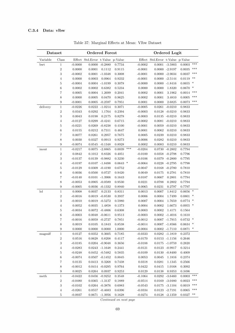
C.3.4 Data: vlbw
Table 37: Marginal Effects at Mean: Vlbw Dataset
Dataset Ordered Forest Ordered Logit
Variable Class Effect Std.Error t-Value p-Value Effect Std.Error t-Value p-Value
bwt 1 -0.0000 0.0000 -0.2880 0.7734 -0.0002 0.0001 -3.5903 0.0003 ***
2 0.0000 0.0001 0.1112 0.9115 -0.0001 0.0000 -2.9197 0.0035 ***
3 -0.0002 0.0001 -1.0348 0.3008 -0.0001 0.0000 -2.9034 0.0037 ***
4 0.0000 0.0003 0.0964 0.9232 -0.0001 0.0000 -2.5144 0.0119 **
5 -0.0004 0.0004 -1.0199 0.3078 -0.0000 0.0000 -1.8416 0.0655 *
6 0.0002 0.0002 0.6382 0.5234 0.0000 0.0000 1.8320 0.0670 *
7 0.0005 0.0004 1.2699 0.2041 0.0002 0.0001 3.1962 0.0014 ***
8 0.0000 0.0005 0.0470 0.9625 0.0002 0.0001 3.4810 0.0005 ***
9 -0.0001 0.0005 -0.2597 0.7951 0.0001 0.0000 2.6825 0.0073 ***
delivery 1 -0.0226 0.0222 -1.0214 0.3071 -0.0005 0.0261 -0.0210 0.9833
2 0.0343 0.0292 1.1764 0.2394 -0.0003 0.0128 -0.0210 0.9833
3 0.0043 0.0198 0.2175 0.8278 -0.0003 0.0135 -0.0210 0.9833
4 -0.0127 0.0299 -0.4241 0.6715 -0.0002 0.0081 -0.0210 0.9833
5 -0.0221 0.0269 -0.8238 0.4100 -0.0001 0.0059 -0.0210 0.9833
6 0.0155 0.0212 0.7311 0.4647 0.0001 0.0062 0.0210 0.9833
7 0.0077 0.0261 0.2957 0.7675 0.0005 0.0239 0.0210 0.9833
8 0.0030 0.0327 0.0913 0.9273 0.0006 0.0282 0.0210 0.9833
9 -0.0074 0.0545 -0.1348 0.8928 0.0002 0.0083 0.0210 0.9833
inout 1 -0.0217 0.0075 -2.8865 0.0039 *** -0.0204 0.0730 -0.2802 0.7794
2 0.0842 0.1012 0.8326 0.4051 -0.0100 0.0358 -0.2798 0.7796
3 -0.0137 0.0139 -0.9882 0.3230 -0.0106 0.0379 -0.2800 0.7795
4 -0.0197 0.0107 -1.8498 0.0643 * -0.0064 0.0228 -0.2795 0.7798
5 -0.0129 0.0309 -0.4190 0.6752 -0.0047 0.0168 -0.2780 0.7810
6 0.0036 0.0500 0.0727 0.9420 0.0049 0.0175 0.2781 0.7810
7 -0.0140 0.0101 -1.3906 0.1643 0.0187 0.0667 0.2801 0.7794
8 -0.0053 0.0905 -0.0589 0.9530 0.0221 0.0788 0.2802 0.7794
9 -0.0005 0.0036 -0.1332 0.8940 0.0065 0.0231 0.2797 0.7797
lol 1 0.0008 0.0037 0.2133 0.8311 0.0013 0.0007 1.8412 0.0656 *
2 -0.0016 0.0019 -0.8530 0.3937 0.0006 0.0004 1.7499 0.0801 *
3 -0.0010 0.0019 -0.5272 0.5980 0.0007 0.0004 1.7659 0.0774 *
4 0.0052 0.0035 1.4858 0.1373 0.0004 0.0002 1.6673 0.0955 *
5 -0.0034 0.0072 -0.4806 0.6308 0.0003 0.0002 1.4171 0.1564
6 -0.0003 0.0048 -0.0611 0.9513 -0.0003 0.0002 -1.4016 0.1610
7 -0.0016 0.0059 -0.2727 0.7851 -0.0012 0.0007 -1.7915 0.0732 *
8 0.0019 0.0105 0.1843 0.8538 -0.0014 0.0007 -1.8566 0.0634 *
9 0.0000 0.0000 0.0000 1.0000 -0.0004 0.0002 -1.7110 0.0871 *
magsulf 1 0.0127 0.0352 0.3605 0.7185 -0.0333 0.0282 -1.1819 0.2372
2 0.0516 0.0628 0.8208 0.4117 -0.0170 0.0153 -1.1156 0.2646
3 -0.0185 0.0204 -0.9048 0.3656 -0.0188 0.0175 -1.0759 0.2820
4 -0.0283 0.0243 -1.1648 0.2441 -0.0121 0.0123 -0.9917 0.3214
5 -0.0248 0.0452 -0.5482 0.5835 -0.0109 0.0130 -0.8400 0.4009
6 -0.0074 0.0507 -0.1452 0.8845 0.0053 0.0045 1.1816 0.2374
7 0.0135 0.0413 0.3268 0.7438 0.0318 0.0281 1.1345 0.2566
8 -0.0012 0.0414 -0.0295 0.9764 0.0422 0.0415 1.0168 0.3092
9 0.0025 0.0264 0.0937 0.9253 0.0129 0.0138 0.9353 0.3496
meth 1 -0.0422 0.0456 -0.9252 0.3548 -0.1064 0.0292 -3.6460 0.0003 ***
2 -0.0480 0.0365 -1.3137 0.1889 -0.0514 0.0169 -3.0480 0.0023 ***
3 -0.0102 0.0264 -0.3876 0.6983 -0.0543 0.0175 -3.1104 0.0019 ***
4 -0.0261 0.0557 -0.4683 0.6396 -0.0334 0.0123 -2.7191 0.0065 ***
5 -0.0937 0.0671 -1.3956 0.1628 -0.0274 0.0128 -2.1359 0.0327 **
Continued on next page
69

Variable Class Effect Std.Error t-Value p-Value Effect Std.Error t-Value p-Value
6 0.0270 0.0502 0.5378 0.5907 0.0183 0.0119 1.5399 0.1236
7 0.1090 0.0595 1.8321 0.0669 * 0.0922 0.0266 3.4649 0.0005 ***
8 0.0743 0.0693 1.0716 0.2839 0.1236 0.0344 3.5942 0.0003 ***
9 0.0099 0.0320 0.3106 0.7561 0.0388 0.0148 2.6263 0.0086 ***
race 1 0.0283 0.0178 1.5959 0.1105 0.0532 0.0259 2.0587 0.0395 **
2 0.0380 0.0199 1.9143 0.0556 * 0.0261 0.0137 1.9025 0.0571 *
3 0.0197 0.0199 0.9883 0.3230 0.0276 0.0147 1.8824 0.0598 *
4 0.0076 0.0406 0.1875 0.8512 0.0166 0.0094 1.7753 0.0759 *
5 -0.0580 0.0570 -1.0182 0.3086 0.0121 0.0080 1.5132 0.1302
6 -0.0047 0.0448 -0.1045 0.9167 -0.0126 0.0087 -1.4496 0.1472
7 -0.0276 0.0471 -0.5853 0.5584 -0.0486 0.0246 -1.9754 0.0482 **
8 -0.0120 0.0489 -0.2460 0.8057 -0.0575 0.0281 -2.0494 0.0404 **
9 0.0087 0.0442 0.1960 0.8446 -0.0168 0.0091 -1.8553 0.0635 *
sex 1 -0.0600 0.0360 -1.6665 0.0956 * 0.0124 0.0238 0.5211 0.6023
2 -0.0243 0.0379 -0.6421 0.5208 0.0061 0.0117 0.5182 0.6043
3 -0.0495 0.0442 -1.1217 0.2620 0.0064 0.0124 0.5169 0.6053
4 0.0891 0.0419 2.1275 0.0334 ** 0.0039 0.0075 0.5122 0.6085
5 0.0051 0.0395 0.1290 0.8974 0.0028 0.0056 0.5008 0.6165
6 -0.0065 0.0401 -0.1615 0.8717 -0.0029 0.0058 -0.5050 0.6136
7 0.0376 0.0419 0.8975 0.3694 -0.0113 0.0219 -0.5177 0.6047
8 0.0023 0.0583 0.0389 0.9690 -0.0134 0.0257 -0.5200 0.6031
9 0.0063 0.0273 0.2317 0.8168 -0.0039 0.0076 -0.5157 0.6060
toc 1 -0.0423 0.0147 -2.8833 0.0039 *** -0.0665 0.0242 -2.7491 0.0060 ***
2 -0.0179 0.0119 -1.5077 0.1316 -0.0345 0.0143 -2.4110 0.0159 **
3 0.0043 0.0162 0.2630 0.7925 -0.0390 0.0162 -2.4091 0.0160 **
4 0.0138 0.0628 0.2193 0.8264 -0.0261 0.0122 -2.1452 0.0319 **
5 0.0111 0.0416 0.2669 0.7896 -0.0261 0.0147 -1.7824 0.0747 *
6 0.0011 0.0385 0.0294 0.9765 0.0057 0.0088 0.6453 0.5188
7 -0.0459 0.0323 -1.4221 0.1550 0.0629 0.0235 2.6741 0.0075 ***
8 0.0662 0.0681 0.9725 0.3308 0.0934 0.0407 2.2964 0.0217 **
9 0.0097 0.0160 0.6044 0.5456 0.0303 0.0158 1.9213 0.0547 *
twn 1 0.0002 0.0321 0.0056 0.9956 -0.0011 0.0298 -0.0374 0.9702
2 -0.0158 0.0147 -1.0786 0.2807 -0.0005 0.0146 -0.0373 0.9702
3 -0.0220 0.0104 -2.1152 0.0344 ** -0.0006 0.0155 -0.0373 0.9703
4 -0.0160 0.0316 -0.5064 0.6126 -0.0003 0.0094 -0.0372 0.9703
5 -0.0090 0.0317 -0.2833 0.7770 -0.0003 0.0069 -0.0370 0.9705
6 0.0196 0.0313 0.6262 0.5312 0.0003 0.0070 0.0376 0.9700
7 0.0436 0.0303 1.4386 0.1503 0.0010 0.0273 0.0373 0.9703
8 0.0046 0.0472 0.0979 0.9220 0.0012 0.0324 0.0372 0.9703
9 -0.0052 0.0231 -0.2239 0.8229 0.0004 0.0095 0.0372 0.9703
Significance levels correspond to: ∗ ∗ ∗. < 0.01, ∗ ∗ . < 0.05, ∗. < 0.1.
Notes: Table shows the comparison of the marginal effects at the covariates means between the Ordered Forest
and the ordered logit. The effects are estimated for all classes, together with the corresponding standard
errors, t-values and p-values. The standard errors for the Ordered Forest are estimated using the weight-based
inference and the standard errors for the ordered logit are obtained via the delta method.
70

Table 38: Mean Marginal Effects: Vlbw Dataset
Dataset Ordered Forest Ordered Logit
Variable Class Effect Std.Error t-Value p-Value Effect Std.Error t-Value p-Value
bwt 1 -0.0001 0.0001 -1.1937 0.2326 -0.0002 0.0001 -3.8018 0.0001 ***
2 0.0001 0.0000 1.7664 0.0773 * -0.0001 0.0000 -3.1300 0.0017 ***
3 -0.0001 0.0001 -1.3585 0.1743 -0.0001 0.0000 -3.0308 0.0024 ***
4 0.0001 0.0001 0.9957 0.3194 -0.0000 0.0000 -2.3930 0.0167 **
5 -0.0001 0.0001 -1.3179 0.1876 -0.0000 0.0000 -1.2067 0.2275
6 -0.0000 0.0001 -0.3389 0.7347 0.0000 0.0000 2.3521 0.0187 **
7 0.0000 0.0001 0.3527 0.7243 0.0001 0.0000 3.4928 0.0005 ***
8 0.0002 0.0002 0.9957 0.3194 0.0002 0.0001 3.5488 0.0004 ***
9 -0.0000 0.0002 -0.0719 0.9427 0.0001 0.0000 2.8356 0.0046 ***
delivery 1 -0.0074 0.0133 -0.5523 0.5807 -0.0006 0.0300 -0.0210 0.9833
2 0.0223 0.0127 1.7486 0.0804 * -0.0002 0.0094 -0.0210 0.9833
3 -0.0049 0.0114 -0.4348 0.6637 -0.0002 0.0078 -0.0210 0.9833
4 -0.0118 0.0124 -0.9522 0.3410 -0.0001 0.0038 -0.0210 0.9833
5 -0.0044 0.0160 -0.2771 0.7817 -0.0000 0.0019 -0.0210 0.9832
6 0.0136 0.0117 1.1587 0.2466 0.0001 0.0036 0.0209 0.9833
7 0.0101 0.0218 0.4601 0.6455 0.0003 0.0129 0.0210 0.9833
8 -0.0107 0.0279 -0.3829 0.7018 0.0005 0.0240 0.0210 0.9833
9 -0.0067 0.0524 -0.1272 0.8988 0.0003 0.0125 0.0210 0.9833
inout 1 -0.0132 0.0038 -3.4819 0.0005 *** -0.0235 0.0838 -0.2804 0.7792
2 0.0432 0.0485 0.8906 0.3731 -0.0074 0.0264 -0.2800 0.7795
3 -0.0053 0.0059 -0.8877 0.3747 -0.0061 0.0219 -0.2799 0.7795
4 -0.0086 0.0035 -2.4568 0.0140 ** -0.0030 0.0106 -0.2789 0.7803
5 -0.0039 0.0090 -0.4380 0.6614 -0.0015 0.0055 -0.2732 0.7847
6 0.0013 0.0234 0.0542 0.9568 0.0028 0.0101 0.2791 0.7802
7 -0.0067 0.0110 -0.6049 0.5453 0.0101 0.0360 0.2801 0.7794
8 -0.0067 0.0475 -0.1409 0.8879 0.0188 0.0670 0.2802 0.7793
9 -0.0001 0.0036 -0.0165 0.9868 0.0098 0.0350 0.2798 0.7796
lol 1 -0.0009 0.0022 -0.4085 0.6829 0.0015 0.0008 1.8907 0.0587 *
2 0.0011 0.0013 0.7964 0.4258 0.0005 0.0003 1.7359 0.0826 *
3 -0.0008 0.0019 -0.4226 0.6726 0.0004 0.0002 1.7377 0.0823 *
4 0.0038 0.0027 1.4203 0.1555 0.0002 0.0001 1.6137 0.1066
5 -0.0015 0.0025 -0.5791 0.5625 0.0001 0.0001 1.0961 0.2730
6 0.0033 0.0021 1.5589 0.1190 -0.0002 0.0001 -1.4960 0.1346
7 0.0006 0.0045 0.1418 0.8872 -0.0006 0.0003 -1.8145 0.0696 *
8 -0.0052 0.0037 -1.3895 0.1647 -0.0012 0.0006 -1.8742 0.0609 *
9 -0.0004 0.0058 -0.0723 0.9424 -0.0006 0.0004 -1.7431 0.0813 *
magsulf 1 -0.0002 0.0195 -0.0126 0.9899 -0.0394 0.0340 -1.1589 0.2465
2 0.0239 0.0282 0.8481 0.3964 -0.0131 0.0123 -1.0700 0.2846
3 -0.0155 0.0165 -0.9342 0.3502 -0.0114 0.0112 -1.0238 0.3059
4 -0.0123 0.0147 -0.8370 0.4026 -0.0059 0.0063 -0.9371 0.3487
5 -0.0052 0.0315 -0.1645 0.8693 -0.0039 0.0052 -0.7447 0.4564
6 0.0076 0.0295 0.2572 0.7971 0.0038 0.0030 1.2364 0.2163
7 0.0144 0.0283 0.5075 0.6118 0.0169 0.0146 1.1512 0.2496
8 -0.0111 0.0181 -0.6092 0.5424 0.0337 0.0313 1.0766 0.2816
9 -0.0016 0.0318 -0.0502 0.9600 0.0194 0.0202 0.9604 0.3369
meth 1 -0.0597 0.0366 -1.6328 0.1025 -0.1146 0.0292 -3.9267 0.0001 ***
2 -0.0108 0.0289 -0.3743 0.7082 -0.0438 0.0151 -2.9102 0.0036 ***
3 -0.0417 0.0270 -1.5428 0.1229 -0.0417 0.0147 -2.8381 0.0045 ***
4 0.0070 0.0331 0.2133 0.8311 -0.0238 0.0096 -2.4647 0.0137 **
5 -0.0652 0.0503 -1.2956 0.1951 -0.0189 0.0096 -1.9593 0.0501 *
6 0.0071 0.0357 0.1989 0.8424 0.0116 0.0083 1.4025 0.1608
7 0.1066 0.0459 2.3208 0.0203 ** 0.0670 0.0219 3.0645 0.0022 ***
Continued on next page
71
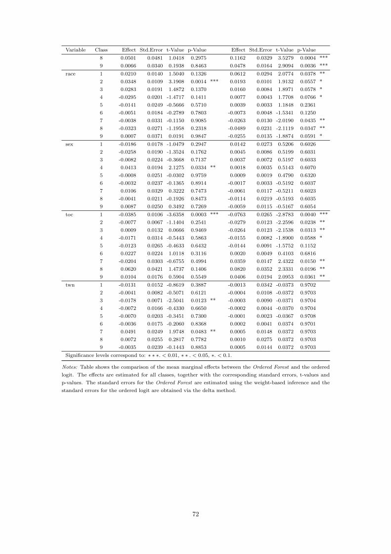
Variable Class Effect Std.Error t-Value p-Value Effect Std.Error t-Value p-Value
8 0.0501 0.0481 1.0418 0.2975 0.1162 0.0329 3.5279 0.0004 ***
9 0.0066 0.0340 0.1938 0.8463 0.0478 0.0164 2.9094 0.0036 ***
race 1 0.0210 0.0140 1.5040 0.1326 0.0612 0.0294 2.0774 0.0378 **
2 0.0348 0.0109 3.1908 0.0014 *** 0.0193 0.0101 1.9132 0.0557 *
3 0.0283 0.0191 1.4872 0.1370 0.0160 0.0084 1.8971 0.0578 *
4 -0.0295 0.0201 -1.4717 0.1411 0.0077 0.0043 1.7708 0.0766 *
5 -0.0141 0.0249 -0.5666 0.5710 0.0039 0.0033 1.1848 0.2361
6 -0.0051 0.0184 -0.2789 0.7803 -0.0073 0.0048 -1.5341 0.1250
7 -0.0038 0.0331 -0.1150 0.9085 -0.0263 0.0130 -2.0190 0.0435 **
8 -0.0323 0.0271 -1.1958 0.2318 -0.0489 0.0231 -2.1119 0.0347 **
9 0.0007 0.0371 0.0191 0.9847 -0.0255 0.0135 -1.8874 0.0591 *
sex 1 -0.0186 0.0178 -1.0479 0.2947 0.0142 0.0273 0.5206 0.6026
2 -0.0258 0.0190 -1.3524 0.1762 0.0045 0.0086 0.5199 0.6031
3 -0.0082 0.0224 -0.3668 0.7137 0.0037 0.0072 0.5197 0.6033
4 0.0413 0.0194 2.1275 0.0334 ** 0.0018 0.0035 0.5143 0.6070
5 -0.0008 0.0251 -0.0302 0.9759 0.0009 0.0019 0.4790 0.6320
6 -0.0032 0.0237 -0.1365 0.8914 -0.0017 0.0033 -0.5192 0.6037
7 0.0106 0.0329 0.3222 0.7473 -0.0061 0.0117 -0.5211 0.6023
8 -0.0041 0.0211 -0.1926 0.8473 -0.0114 0.0219 -0.5193 0.6035
9 0.0087 0.0250 0.3492 0.7269 -0.0059 0.0115 -0.5167 0.6054
toc 1 -0.0385 0.0106 -3.6358 0.0003 *** -0.0763 0.0265 -2.8783 0.0040 ***
2 -0.0077 0.0067 -1.1404 0.2541 -0.0279 0.0123 -2.2596 0.0238 **
3 0.0009 0.0132 0.0666 0.9469 -0.0264 0.0123 -2.1538 0.0313 **
4 -0.0171 0.0314 -0.5443 0.5863 -0.0155 0.0082 -1.8900 0.0588 *
5 -0.0123 0.0265 -0.4633 0.6432 -0.0144 0.0091 -1.5752 0.1152
6 0.0227 0.0224 1.0118 0.3116 0.0020 0.0049 0.4103 0.6816
7 -0.0204 0.0303 -0.6755 0.4994 0.0359 0.0147 2.4322 0.0150 **
8 0.0620 0.0421 1.4737 0.1406 0.0820 0.0352 2.3331 0.0196 **
9 0.0104 0.0176 0.5904 0.5549 0.0406 0.0194 2.0953 0.0361 **
twn 1 -0.0131 0.0152 -0.8619 0.3887 -0.0013 0.0342 -0.0373 0.9702
2 -0.0041 0.0082 -0.5071 0.6121 -0.0004 0.0108 -0.0372 0.9703
3 -0.0178 0.0071 -2.5041 0.0123 ** -0.0003 0.0090 -0.0371 0.9704
4 -0.0072 0.0166 -0.4330 0.6650 -0.0002 0.0044 -0.0370 0.9704
5 -0.0070 0.0203 -0.3451 0.7300 -0.0001 0.0023 -0.0367 0.9708
6 -0.0036 0.0175 -0.2060 0.8368 0.0002 0.0041 0.0374 0.9701
7 0.0491 0.0249 1.9748 0.0483 ** 0.0005 0.0148 0.0372 0.9703
8 0.0072 0.0255 0.2817 0.7782 0.0010 0.0275 0.0372 0.9703
9 -0.0035 0.0239 -0.1443 0.8853 0.0005 0.0144 0.0372 0.9703
Significance levels correspond to: ∗ ∗ ∗. < 0.01, ∗ ∗ . < 0.05, ∗. < 0.1.
Notes: Table shows the comparison of the mean marginal effects between the Ordered Forest and the ordered
logit. The effects are estimated for all classes, together with the corresponding standard errors, t-values and
p-values. The standard errors for the Ordered Forest are estimated using the weight-based inference and the
standard errors for the ordered logit are obtained via the delta method.
72
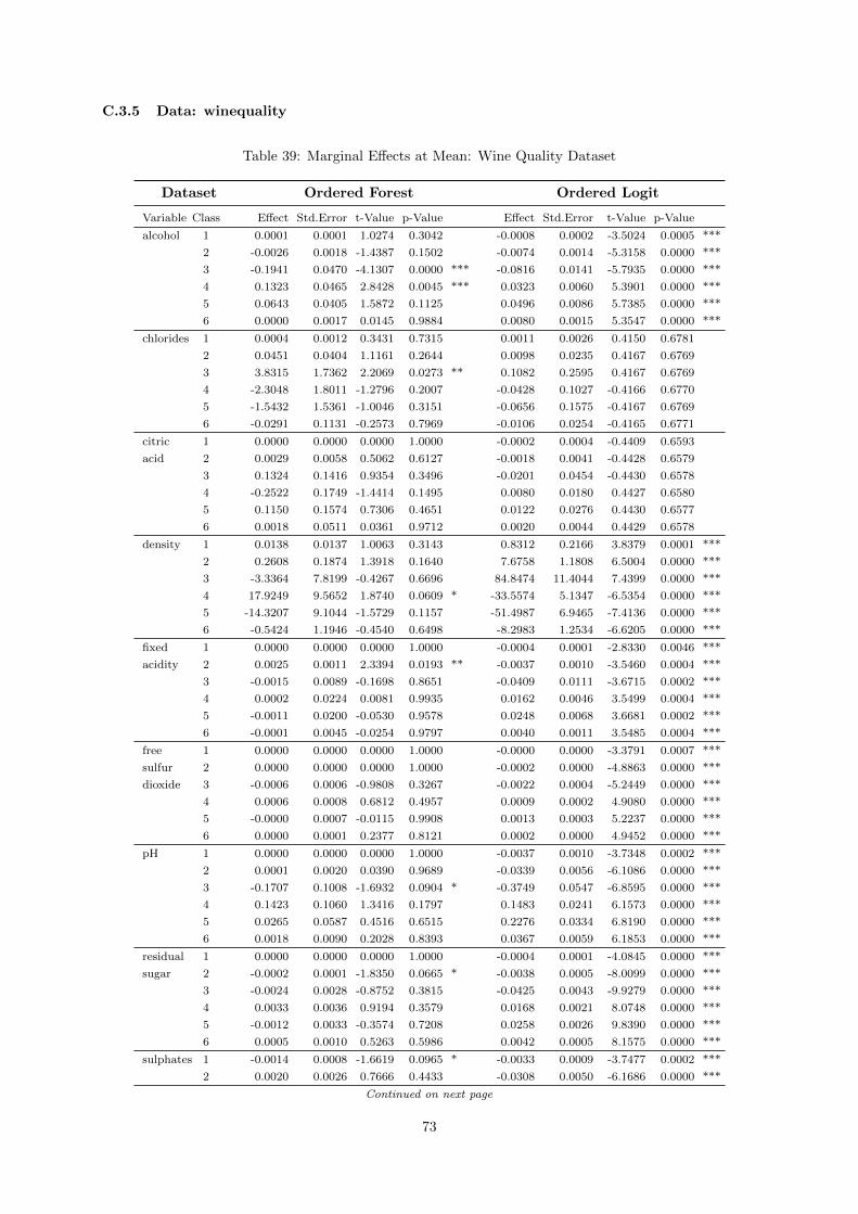
C.3.5 Data: winequality
Table 39: Marginal Effects at Mean: Wine Quality Dataset
Dataset Ordered Forest Ordered Logit
Variable Class Effect Std.Error t-Value p-Value Effect Std.Error t-Value p-Value
alcohol 1 0.0001 0.0001 1.0274 0.3042 -0.0008 0.0002 -3.5024 0.0005 ***
2 -0.0026 0.0018 -1.4387 0.1502 -0.0074 0.0014 -5.3158 0.0000 ***
3 -0.1941 0.0470 -4.1307 0.0000 *** -0.0816 0.0141 -5.7935 0.0000 ***
4 0.1323 0.0465 2.8428 0.0045 *** 0.0323 0.0060 5.3901 0.0000 ***
5 0.0643 0.0405 1.5872 0.1125 0.0496 0.0086 5.7385 0.0000 ***
6 0.0000 0.0017 0.0145 0.9884 0.0080 0.0015 5.3547 0.0000 ***
chlorides 1 0.0004 0.0012 0.3431 0.7315 0.0011 0.0026 0.4150 0.6781
2 0.0451 0.0404 1.1161 0.2644 0.0098 0.0235 0.4167 0.6769
3 3.8315 1.7362 2.2069 0.0273 ** 0.1082 0.2595 0.4167 0.6769
4 -2.3048 1.8011 -1.2796 0.2007 -0.0428 0.1027 -0.4166 0.6770
5 -1.5432 1.5361 -1.0046 0.3151 -0.0656 0.1575 -0.4167 0.6769
6 -0.0291 0.1131 -0.2573 0.7969 -0.0106 0.0254 -0.4165 0.6771
citric 1 0.0000 0.0000 0.0000 1.0000 -0.0002 0.0004 -0.4409 0.6593
acid 2 0.0029 0.0058 0.5062 0.6127 -0.0018 0.0041 -0.4428 0.6579
3 0.1324 0.1416 0.9354 0.3496 -0.0201 0.0454 -0.4430 0.6578
4 -0.2522 0.1749 -1.4414 0.1495 0.0080 0.0180 0.4427 0.6580
5 0.1150 0.1574 0.7306 0.4651 0.0122 0.0276 0.4430 0.6577
6 0.0018 0.0511 0.0361 0.9712 0.0020 0.0044 0.4429 0.6578
density 1 0.0138 0.0137 1.0063 0.3143 0.8312 0.2166 3.8379 0.0001 ***
2 0.2608 0.1874 1.3918 0.1640 7.6758 1.1808 6.5004 0.0000 ***
3 -3.3364 7.8199 -0.4267 0.6696 84.8474 11.4044 7.4399 0.0000 ***
4 17.9249 9.5652 1.8740 0.0609 * -33.5574 5.1347 -6.5354 0.0000 ***
5 -14.3207 9.1044 -1.5729 0.1157 -51.4987 6.9465 -7.4136 0.0000 ***
6 -0.5424 1.1946 -0.4540 0.6498 -8.2983 1.2534 -6.6205 0.0000 ***
fixed 1 0.0000 0.0000 0.0000 1.0000 -0.0004 0.0001 -2.8330 0.0046 ***
acidity 2 0.0025 0.0011 2.3394 0.0193 ** -0.0037 0.0010 -3.5460 0.0004 ***
3 -0.0015 0.0089 -0.1698 0.8651 -0.0409 0.0111 -3.6715 0.0002 ***
4 0.0002 0.0224 0.0081 0.9935 0.0162 0.0046 3.5499 0.0004 ***
5 -0.0011 0.0200 -0.0530 0.9578 0.0248 0.0068 3.6681 0.0002 ***
6 -0.0001 0.0045 -0.0254 0.9797 0.0040 0.0011 3.5485 0.0004 ***
free 1 0.0000 0.0000 0.0000 1.0000 -0.0000 0.0000 -3.3791 0.0007 ***
sulfur 2 0.0000 0.0000 0.0000 1.0000 -0.0002 0.0000 -4.8863 0.0000 ***
dioxide 3 -0.0006 0.0006 -0.9808 0.3267 -0.0022 0.0004 -5.2449 0.0000 ***
4 0.0006 0.0008 0.6812 0.4957 0.0009 0.0002 4.9080 0.0000 ***
5 -0.0000 0.0007 -0.0115 0.9908 0.0013 0.0003 5.2237 0.0000 ***
6 0.0000 0.0001 0.2377 0.8121 0.0002 0.0000 4.9452 0.0000 ***
pH 1 0.0000 0.0000 0.0000 1.0000 -0.0037 0.0010 -3.7348 0.0002 ***
2 0.0001 0.0020 0.0390 0.9689 -0.0339 0.0056 -6.1086 0.0000 ***
3 -0.1707 0.1008 -1.6932 0.0904 * -0.3749 0.0547 -6.8595 0.0000 ***
4 0.1423 0.1060 1.3416 0.1797 0.1483 0.0241 6.1573 0.0000 ***
5 0.0265 0.0587 0.4516 0.6515 0.2276 0.0334 6.8190 0.0000 ***
6 0.0018 0.0090 0.2028 0.8393 0.0367 0.0059 6.1853 0.0000 ***
residual 1 0.0000 0.0000 0.0000 1.0000 -0.0004 0.0001 -4.0845 0.0000 ***
sugar 2 -0.0002 0.0001 -1.8350 0.0665 * -0.0038 0.0005 -8.0099 0.0000 ***
3 -0.0024 0.0028 -0.8752 0.3815 -0.0425 0.0043 -9.9279 0.0000 ***
4 0.0033 0.0036 0.9194 0.3579 0.0168 0.0021 8.0748 0.0000 ***
5 -0.0012 0.0033 -0.3574 0.7208 0.0258 0.0026 9.8390 0.0000 ***
6 0.0005 0.0010 0.5263 0.5986 0.0042 0.0005 8.1575 0.0000 ***
sulphates 1 -0.0014 0.0008 -1.6619 0.0965 * -0.0033 0.0009 -3.7477 0.0002 ***
2 0.0020 0.0026 0.7666 0.4433 -0.0308 0.0050 -6.1686 0.0000 ***
Continued on next page
73
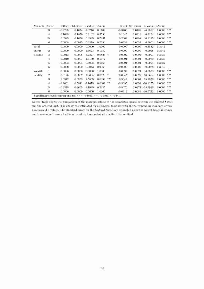
Variable Class Effect Std.Error t-Value p-Value Effect Std.Error t-Value p-Value
3 -0.2295 0.1674 -1.3716 0.1702 -0.3400 0.0489 -6.9592 0.0000 ***
4 0.1695 0.1850 0.9162 0.3596 0.1345 0.0216 6.2134 0.0000 ***
5 0.0585 0.1656 0.3535 0.7237 0.2064 0.0298 6.9195 0.0000 ***
6 0.0008 0.0025 0.3379 0.7354 0.0333 0.0053 6.3001 0.0000 ***
total 1 0.0000 0.0000 0.0000 1.0000 0.0000 0.0000 0.8882 0.3744
sulfur 2 -0.0000 0.0000 -1.5623 0.1182 0.0000 0.0000 0.9068 0.3645
dioxide 3 0.0013 0.0008 1.7377 0.0823 * 0.0002 0.0002 0.9097 0.3630
4 -0.0010 0.0007 -1.4130 0.1577 -0.0001 0.0001 -0.9080 0.3639
5 -0.0003 0.0005 -0.5008 0.6165 -0.0001 0.0001 -0.9094 0.3632
6 0.0000 0.0000 0.0043 0.9965 -0.0000 0.0000 -0.9078 0.3640
volatile 1 0.0000 0.0000 0.0000 1.0000 0.0092 0.0021 4.3528 0.0000 ***
acidity 2 0.0125 0.0067 1.8604 0.0628 * 0.0845 0.0079 10.6684 0.0000 ***
3 1.6912 0.6553 2.5809 0.0099 *** 0.9342 0.0604 15.4576 0.0000 ***
4 -1.2661 0.5841 -2.1675 0.0302 ** -0.3695 0.0354 -10.4275 0.0000 ***
5 -0.4375 0.3665 -1.1939 0.2325 -0.5670 0.0371 -15.2936 0.0000 ***
6 0.0000 0.0000 0.0000 1.0000 -0.0914 0.0089 -10.2723 0.0000 ***
Significance levels correspond to: ∗ ∗ ∗. < 0.01, ∗ ∗ . < 0.05, ∗. < 0.1.
Notes: Table shows the comparison of the marginal effects at the covariates means between the Ordered Forest
and the ordered logit. The effects are estimated for all classes, together with the corresponding standard errors,
t-values and p-values. The standard errors for the Ordered Forest are estimated using the weight-based inference
and the standard errors for the ordered logit are obtained via the delta method.
74

![Exploring Categorical Structuralismcase.edu/artsci/phil/PMExploring.pdfExploring Categorical Structuralism COLIN MCLARTY* Hellman [2003] raises interesting challenges to categorical](https://img.pdfslide.us/doc/110x75/5b04a7507f8b9a4e538e151c/exploring-categorical-categorical-structuralism-colin-mclarty-hellman-2003-raises.jpg)


![Bayesian multinomial ordered categorical response model …50 ordered categorical data [17; 18]. 51 Cumulative models, as discussed in [19–21], are widely used regression model for](https://img.pdfslide.us/doc/110x75/6120b07171c6373ae369ab78/bayesian-multinomial-ordered-categorical-response-model-50-ordered-categorical-data.jpg)