Embed Size (px)
Citation preview
Applied and Computational Harmonic Analysis 11, 89–123 (2001)doi:10.1006/acha.2000.0350, available online at http://www.idealibrary.com on
Random Cascades on Wavelet Trees and Their Usein Analyzing and Modeling Natural Images
Martin J. Wainwright 1
Laboratory for Information and Decision Systems, Electrical Engineering and Computer Science,Massachusetts Institute of Technology, Cambridge, Massachusetts 02139
E-mail: [email protected]
Eero P. Simoncelli 2
Center for Neural Science, Courant Institute of Mathematical Sciences, New York University, New York,
New York 10012E-mail: [email protected]
and
Alan S. Willsky 1
Laboratory for Information and Decision Systems, Electrical Engineering and Computer Science,
Massachusetts Institute of Technology, Cambridge, Massachusetts 02139E-mail: [email protected]
We develop a new class of non-Gaussian multiscale stochastic processes definedby random cascades on trees of multiresolution coefficients. These cascadesreproduce a semiparametric class of random variables known as Gaussian scalemixtures, members of which include many of the best known, heavy-taileddistributions. This class of cascade models is rich enough to accurately capturethe remarkably regular and non-Gaussian features of natural images, but alsosufficiently structured to permit the development of efficient algorithms. Inparticular, we develop an efficient technique for estimation, and demonstrate in adenoising application that it preserves natural image structure (e.g., edges). Ourframework generates global yet structured image models, thereby providing aunified basis for a variety of applications in signal and image processing, includingimage denoising, coding, and super-resolution. 2001 Academic Press
1. INTRODUCTION
Stochastic models of natural images underlie a variety of applications in imageprocessing and low-level computer vision, including image coding, denoising and
1 MW supported by NSERC 1967 fellowship; AW and MW by AFOSR Grant F49620-98-1-0349 and ONRGrant N00014-91-J-1004. Address correspondence to MW.
2 ES supported by NSF Career Grant MIP-9796040 and an Alfred P. Sloan fellowship.
89
1063-5203/01 $35.00Copyright 2001 by Academic Press
All rights of reproduction in any form reserved.
90 WAINWRIGHT, SIMONCELLI, AND WILLSKY
restoration, interpolation and synthesis. Accordingly, the past decade has witnessedan increasing amount of research devoted to developing stochastic models of images(e.g., [19, 38, 45, 48, 55]). Simultaneously, wavelet transforms and other multiresolutionrepresentations have profoundly influenced image processing and low-level computervision (e.g., [34]). Moreover, multiscale theory has proven useful in modeling andsynthesizing a variety of stochastic processes (e.g., [12, 33, 60]).
The intersection of these three lines of research—statistical image models, multiscalerepresentations, and multiscale modeling of stochastic processes—constitute the focus ofthis paper. More specifically, our goal is to develop and study a new class of multiscalestochastic processes that are capable of capturing the statistics of natural images. Theseprocesses are defined by random coarse-to-fine cascades on trees of wavelet or othermultiresolution coefficients. Our cascade models represent a significant variation on linearmodels defined on multiscale trees (e.g., [8]). Although such models lead to exceptionallyefficient algorithms for image processing, their linear nature means that they cannot capturethe striking types of non-Gaussian behavior present in wavelet pyramids of natural images.To capture such behavior, we define random cascades that reproduce a rich semiparametricclass of random variables known as Gaussian scale mixtures (GSMs). We demonstrate thatthe structure of our random cascade models not only captures natural image statistics, butalso facilitates efficient and optimal processing, which we illustrate by application to imagedenoising. Preliminary forms of parts of this work have appeared in [56, 57].
1.1. The Statistics of Natural Images
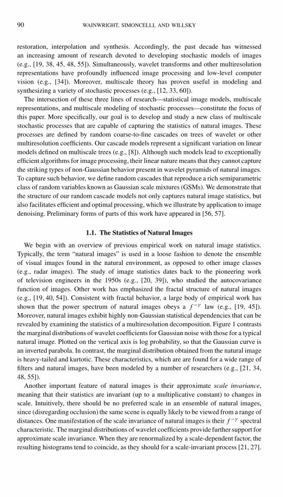
We begin with an overview of previous empirical work on natural image statistics.Typically, the term “natural images” is used in a loose fashion to denote the ensembleof visual images found in the natural environment, as opposed to other image classes(e.g., radar images). The study of image statistics dates back to the pioneering workof television engineers in the 1950s (e.g., [20, 39]), who studied the autocovariancefunction of images. Other work has emphasized the fractal structure of natural images(e.g., [19, 40, 54]). Consistent with fractal behavior, a large body of empirical work hasshown that the power spectrum of natural images obeys a f−γ law (e.g., [19, 45]).Moreover, natural images exhibit highly non-Gaussian statistical dependencies that can berevealed by examining the statistics of a multiresolution decomposition. Figure 1 contraststhe marginal distributions of wavelet coefficients for Gaussian noise with those for a typicalnatural image. Plotted on the vertical axis is log probability, so that the Gaussian curve isan inverted parabola. In contrast, the marginal distribution obtained from the natural imageis heavy-tailed and kurtotic. These characteristics, which are are found for a wide range offilters and natural images, have been modeled by a number of researchers (e.g., [21, 34,48, 55]).
Another important feature of natural images is their approximate scale invariance,meaning that their statistics are invariant (up to a multiplicative constant) to changes inscale. Intuitively, there should be no preferred scale in an ensemble of natural images,since (disregarding occlusion) the same scene is equally likely to be viewed from a range ofdistances. One manifestation of the scale invariance of natural images is their f−γ spectralcharacteristic. The marginal distributions of wavelet coefficients provide further support forapproximate scale invariance. When they are renormalized by a scale-dependent factor, theresulting histograms tend to coincide, as they should for a scale-invariant process [21, 27].
RANDOM CASCADES ON WAVELET TREES 91
FIG. 1. Histograms of wavelet marginal distributions for (a) Gaussian noise; and (b) a typical natural image.Vertical axis gives log probability (rescaled).
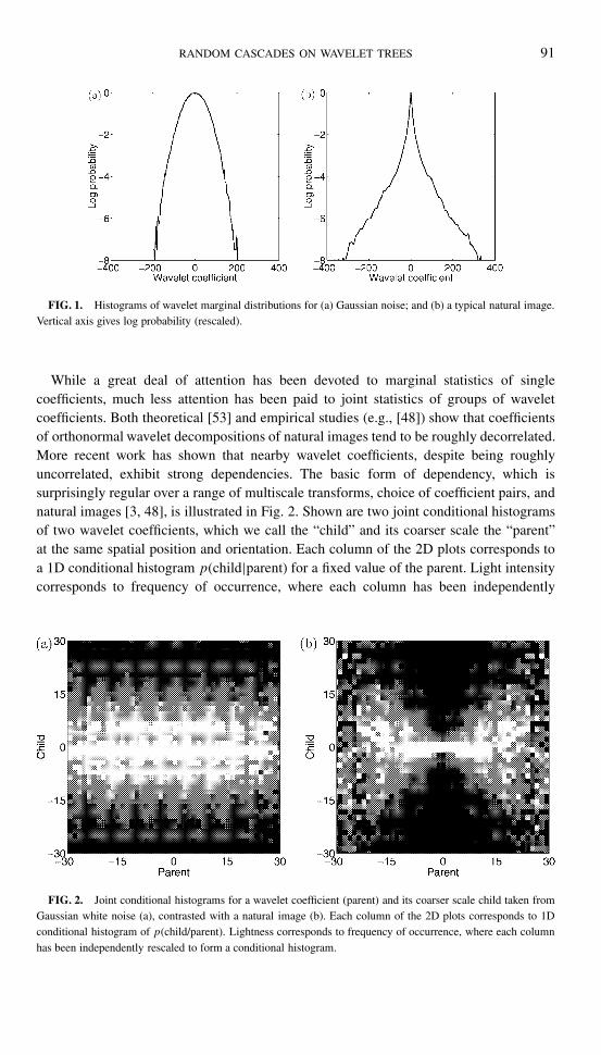
While a great deal of attention has been devoted to marginal statistics of singlecoefficients, much less attention has been paid to joint statistics of groups of waveletcoefficients. Both theoretical [53] and empirical studies (e.g., [48]) show that coefficientsof orthonormal wavelet decompositions of natural images tend to be roughly decorrelated.More recent work has shown that nearby wavelet coefficients, despite being roughlyuncorrelated, exhibit strong dependencies. The basic form of dependency, which issurprisingly regular over a range of multiscale transforms, choice of coefficient pairs, andnatural images [3, 48], is illustrated in Fig. 2. Shown are two joint conditional histogramsof two wavelet coefficients, which we call the “child” and its coarser scale the “parent”at the same spatial position and orientation. Each column of the 2D plots corresponds toa 1D conditional histogram p(child|parent) for a fixed value of the parent. Light intensitycorresponds to frequency of occurrence, where each column has been independently
FIG. 2. Joint conditional histograms for a wavelet coefficient (parent) and its coarser scale child taken fromGaussian white noise (a), contrasted with a natural image (b). Each column of the 2D plots corresponds to 1Dconditional histogram of p(child/parent). Lightness corresponds to frequency of occurrence, where each columnhas been independently rescaled to form a conditional histogram.
92 WAINWRIGHT, SIMONCELLI, AND WILLSKY
rescaled to form a conditional histogram. Panel (a) corresponds to a Gaussian white noiseimage. As expected, the two coefficients are independent, because the shape of the cross-section p(child|parent) is independent of the value of the parent.
In contrast, panel (b) shows typical behavior for a natural image. Although thetwo wavelet coefficients are approximately decorrelated, they are highly dependent. Inparticular, the distribution of the child conditioned on the value of the parent has a standarddeviation that scales with the absolute value of the parent. The characteristic “bow tie”shape of this histogram is found for wavelet coefficients at nearby spatial positions,adjacent orientations and spatial scales, and over a wide range of natural images. Thus,wavelet coefficients from natural images exhibit a striking self-reinforcing characteristic, inthat if one wavelet coefficient is large in absolute value, then “nearby” coefficients (wherenearness is measured in scale, position, or orientation) also are more likely to be large inabsolute value.
1.2. Overview
The previous section laid out a number of striking empirical characteristics that shouldbe reproduced by a stochastic model for images. The goals of this paper are to developa mathematical framework for capturing the structure of natural images and to showthat it can be used as the consistent basis for a variety of image processing tasks. Aswith other work on natural images (e.g., [21, 43, 48]), we work in terms of wavelet orother multiresolution coefficients, which can be identified with the nodes of a multiscaletree. The basis of our approach is the decomposition of wavelet coefficients into twounderlying stochastic processes defined on the multiscale tree. In particular, we modelwavelet coefficients as a product of one white multiscale Gaussian process with a secondcontinuous-valued multiplier process. This multiplier process, which is generated asa nonlinear function of a second Gaussian multiscale process (called the premultiplier),serves to control the non-Gaussian dependencies among wavelet coefficients.
The class of marginal distributions generated by this nonlinear mixing is rich, includingmany of the best known and well-studied heavy-tailed variables. Moreover, the multiscaletree structure allows us to construct global probability distributions on all waveletcoefficients, and hence statistical models for natural images. We show that this frameworkis powerful enough to capture the key characteristics of natural images described above;moreover, it does so in a parsimonious fashion, requiring only a small set of parameters.Both Gaussian processes in the underlying decomposition are modeled by the multiscaleframework of [8, 33], which permits efficient and optimal algorithms. As a result, althoughour models produce highly non-Gaussian statistics, we are able to exploit this embeddedlinear-Gaussian structure to great advantage. A number of other researchers (e.g., [21, 43,44, 48, 54]) have studied and exploited the properties of natural images on which wefocus here, and our approach has both some similarities and important differences withthese earlier efforts. Later in the paper, we discuss these links both in image modeling(Section 3.4) and in image denoising and coding (Section 4.2). We also note that similarmodels also been studied in speech processing (e.g., [62]) and financial mathematics(e.g., [63]).
In next section, we provide the mathematical preliminaries for our treatment, includingan introduction to and some new results concerning so-called Gaussian scale mixtures.
RANDOM CASCADES ON WAVELET TREES 93
We also briefly review the relevant features of the linear multiscale modeling frameworkin (e.g., [8, 33]). In Section 3, we introduce the class of multiscale wavelet cascade modelsand illustrate the characteristics that can be captured by such models, including the highlynon-Gaussian structure of natural images. In Section 4, we develop an algorithm formaximum a posteriori (MAP) estimation of the premultiplier process. On the basis ofthis estimator, we develop a technique for image denoising that preserves the structureof natural images. In addition, we describe an algorithm for estimating model parameters.Section 5 provides illustrative results of applying the wavelet denoising algorithm to both1D signals and natural images. Section 6 summarizes our work, and points out directionsfor future work.
2. MATHEMATICAL PRELIMINARIES
This section develops mathematical preliminaries necessary for defining randomcascades on wavelet trees. We begin by introducing the semiparametric class of randomvariables known as Gaussian scale mixtures and providing some analysis of their propertiesrequired for our development. We end by reviewing the relevant aspects of previous workon linear multiscale stochastic processes.
2.1. Gaussian Scale Mixtures
In this section, we introduce and describe some of the basic properties of GSMs,including several new results whose proofs can be found in Appendix A. To begin, aGSM vector c is formed by taking the product of two independent random variables,namely a positive scalar random variable z known as the multiplier or mixing variableand a Gaussian random vector u distributed as 3 N (0,�). With this notation, we havecd= √
zu, whered= denotes equality in distribution.
The choice of mixing variable specifies the GSM variable c with associated GSMdensity pc. In particular, the GSM density can be represented as an integral of a Gaussiankernel function scaled and weighted by the mixing variable
pc(c)=∫ ∞
0
1
(2π)m/2|z�|1/2 exp
(−cT �−1c
2z
)pz(z) dz, (1)
where pz is the density of the mixing variable, and m is the dimension of the randomvector c. As a special case, the finite mixture of Gaussians corresponds to choosing pz tobe a (discrete) probability mass function, in which case the integral reduces to a finite sum.
A first question concerns characterizing which random vectors can be represented asGSMs. For simplicity in notation, we focus on the case of a scalar GSM, althoughthe results can be stated more generally. We begin with a few definitions. First ofall, recall that the characteristic function of a random variable c is given by φc(s) =∫ ∞−∞ exp(ics)pc(c) dc, where pc is the density function of c. We also need the notion
of complete monotonicity: a function f defined on (0,∞) is completely monotone if it hasderivatives f (n) of all orders, and (−1)n f (n)(y)≥ 0 for all y > 0 and n= 0,1,2, . . . . With
3 The notation x ∼N (µ,�) means that x is distributed as a Gaussian with mean µ and covariance �.
94 WAINWRIGHT, SIMONCELLI, AND WILLSKY
these definitions, we have the following necessary and sufficient conditions:
THEOREM 1. A symmetric random variable c with characteristic function φc(t) isa GSM if and only if g(s)� φc(
√s ) is completely monotone.
Proof. See Appendix A.
Andrews and Mallows [1] provide the following necessary and sufficient conditions onthe density function:
THEOREM 2. Let c have a density function pc that is symmetric about zero. Then c isa GSM if and only if f (y)� pc(
√y ) is completely monotone.
These two theorems provide straightforward criteria for a GSM in the characteristicfunction and density domains respectively.
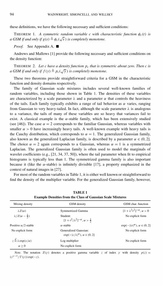
The family of Gaussian scale mixtures includes several well-known families ofrandom variables, including those shown in Table 1. The densities of these variablesare characterized by a scale parameter λ and a parameter α that controls the heavinessof the tails. Each family typically exhibits a range of tail behavior as α varies, rangingfrom Gaussian to very heavy-tailed. In fact, although the scale parameter λ is analogousto a variance, the tails of many of these variables are so heavy that variances fail toexist. A classical example is the α-stable family, which has been extensively studied(see [46]). The case α = 2 corresponds to the familiar Gaussian, whereas variables withsmaller α > 0 have increasingly heavy tails. A well-known example with heavy tails isthe Cauchy distribution, which corresponds to α = 1. The generalized Gaussian family,also known as the generalized Laplacian family, is described by a parameter α ∈ (0,2].The choice α = 2 again corresponds to a Gaussian, whereas α = 1 is a symmetrizedLaplacian. The generalized Gaussian family is often used to model the marginals ofwavelet coefficients (e.g., [21, 34, 37, 50]), where the tail parameter when fit to empiricalhistograms is typically less than 1. The symmetrized gamma family is also importantbecause it (like the α-stable) is infinitely divisible [17], a property emphasized in thecontext of natural images in [27].
For most of the random variables in Table 1, it is either well known or straightforward tofind the density of the multiplier variable. For the generalized Gaussian family, however,
TABLE 1Example Densities from the Class of Gaussian Scale Mixtures
Mixing density GSM density GSM char. function
λZ(α) Symmetrized Gamma [1 + λ2t2]−α , α > 0
λ/Z(α− 12 ) Student: No explicit form
[1 + t2/λ2]−α , α > 12
Positive α/2-stable α-stable exp(−|λt|α), α ∈ (0,2]No explicit form Generalized Gaussian: No explicit form
exp(−|c/λ|α), α ∈ (0,2]zd= λexp(x/α) Log multiplier No explicit form
α ≥ 0 No explicit form
Note. The notation Z(γ ) denotes a positive gamma variable z of index γ with density p(z) =(zγ−1/�(γ )) exp(−z).
RANDOM CASCADES ON WAVELET TREES 95
this verification is not entirely straightforward. In order to show that the generalizedGaussian is a GSM, we first need to formally develop a relation apparent in Table 1(e.g., compare symmetrized gamma and generalized Student variables).
THEOREM 3. Let cd= √
zu be a GSM with characteristic function φc, and letthe mixing variable z have density pz. Define f (v) � pz(v)/
√v, and suppose that∫ ∞
0 f (v) dv <∞, in which case we can consider a random variable v with the density f .
Then the GSM yd= (1/√v)u has density py(y)∝ φc(y).
Proof. See Appendix A.
On the basis of Theorem 3, one would conjecture that the generalized Gaussian family
should have a representation cd= (1/
√v)u, with the density of v satisfying f (v) ∝
pα/2(v)/√v, where pα/2 is the density of a positive α/2-stable random variable. In order
to prove this conjecture, it is necessary to verify that f (as defined above) is a valid densityfunction: i.e., that
∫ ∞0 f (v) dv < ∞. This verification is not entirely straightforward,
because with certain exceptions (e.g., α = 12 ), there are no explicit forms for the positive
α-stable densities. Nonetheless, it can be proved by using properties of positive α-stabledensities [17], and we summarize the results in the following:
PROPOSITION 1. The generalized Gaussian family has the representation cd=
(1/√v)u, where in particular, v has the density proportional to pα/2(v)/
√v, and pα/2 is
the density of a positive α/2-stable variable.
Proof. See Appendix A.
In this paper, we will frequently exploit the fact that a large class of nonnegativemultipliers z can be generated by passing a Gaussian random variable z through theappropriate function h: R → R
+. The following result characterizes those GSMs that canbe represented in this way:
PROPOSITION 2. Let cd= √
zu be a GSM, and suppose that the cumulative distributionfunction (CDF) F of the multiplier is invertible. Then c has an equivalent representation
cd= h(x)u for an appropriate function h: R → R
+, where x ∼N (0,1).
Proof. Let F and G be the CDFs of z and x respectively. Since the inverse function
F−1: [0,1] → R+ is defined, we have z
d= F−1(G(x)), and h(x)� [F−1(G(x))]1/2 is theappropriate function.
According to this representation, the multiplier z is given by h2(x). We refer to theGaussian quantity x as the premultiplier since it is the stochastic input to the nonlinearity hthat generates the multiplier. The conditions of Proposition 2 (i.e., invertible cumulativedistribution function F ) will be satisfied under a variety of conditions, including when thedensity pz is nowhere zero on (0,∞). This latter condition includes all random variableslisted in Table 1.
In many cases, it is possible to determine explicitly the form of h. For example, choosingh(x)= |x| will generate the square root of gamma variables of index 1/2, which allows usto produce the symmetrized gamma variable of index 1/2. For the purpose of application,the precise form of GSM may not be critical. In this context, an advantage of the GSMframework is that it does not require an explicit form of the density of c, but instead focuses
96 WAINWRIGHT, SIMONCELLI, AND WILLSKY
attention on the multiplier. Our set-up allows an arbitrary choice of the nonlinearity h,meaning that it permits the use of GSMs which may confer a computational or analyticaladvantage. For the results in this paper, we will choose h from parameterized familiesof functions that generate random variables with ranges of behavior. One example is thefamily of functions {(exp(x/α) | α > 0}, orresponding to the lognormal family listed inTable 1. Another choice is the family {(x+)α | α > 0}, which generates a class of variableswith a range of tail behavior that is qualitatively similar to the symmetrized gamma andgeneralized Gaussian families. 4
The GSM class includes many random variables with tails so heavy that variances andlower moments may fail to exist. Such variables are characterized by polynomial decay inthe tails of the distribution, where the prototypical example is the α-stable family for α < 2.Polynomially decaying tails are not appropriate for modeling the wavelet coefficientsof natural images, for which the tails tend to drop off more quickly. Therefore, for theapplications to natural images in this paper, we consider GSMs for which variances exist.Such variables can still exhibit highly non-Gaussian tail behavior, as will be clear in ourmodeling of wavelet marginal densities.
2.2. Multiscale Stochastic Processes
In this section, we introduce some of the basic concepts and results concerning linearmultiscale models defined on trees. We limit our treatment to those aspects required forsubsequent development; the reader is referred to other literature (e.g., [8, 12, 18, 33] forfurther details of these models, and their application to a variety of 1-D and 2-D statisticalinference problems.
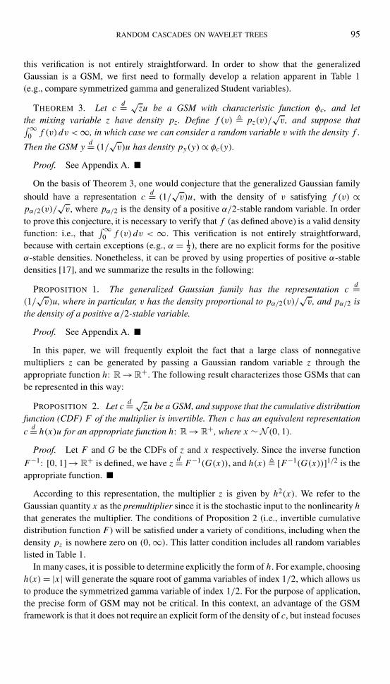
The processes of interest to us are defined on a tree T , such as that illustrated inFig. 3. The nodes s ∈ T are organized, as depicted in the figure, into a series of scales,which we enumerate m = 0,1, . . . ,M . At the coarsest scale m = 0 (the top of the tree)there is a single node s = 0, which we designate the root node. At the next finest scalem = 1 are q nodes, which correspond to the children of the root node. We specializehere to regular trees, so that each parent node has the same number of children (q). Thisprocedure of moving from parent to child is then applied recursively, so that a node at scalem<M gives birth to q children at the next scale (m+ 1). These children are indexed bysα1, . . . , sαq . Similarly, each node s at scalem> 0 has a unique parent sγ at scale (m−1).
4 Here the notation x+ denotes the positive part of x, defined by x+ = x for x ≥ 0 and 0 otherwise.
FIG. 3. A segment of a q-adic tree, with the unique parent sγ and children sαq, . . . , sαq corresponding tonode s .
RANDOM CASCADES ON WAVELET TREES 97
It should be noted that such trees arise naturally from multiresolution decompositions. Forinstance, a wavelet decomposition of a 1D signal generates a binary tree (q = 2), whereasdecomposing an image will generate a quadtree (q = 4).
To define a multiscale stochastic process, we assign to each node of the tree a randomvector x(s). The processes of interest to us are a particular class that are Markovwith respect to the graph structure of the tree. In particular, a multiscale Markov treeprocess x(s), s ∈ T has the property that for any two distinct nodes s, t ∈ T , x(s) and x(t)are conditionally independent given x(τ) at any node τ on the unique path from s to t . Forexample, if we define s∧ t as the coarsest scale node on this path (also the nearest commonancestor of s and t), then x(s) and x(t) are independent given x(s ∧ t).
Multiscale processes in which the random variables x(s) at each node assume a discreteset of values represent a generalization of the usual (discrete) Markov chain to moregeneral tree graphs. A number of researchers have studied and made use of such discretemultiscale processes (e.g., [7, 10]). Of particular relevance here is the work of Baraniuk andcolleagues [10, 43], who have used such discrete multiscale stochastic processes as part oftheir non-Gaussian modeling framework for signal and image processing. In Section 3.4,we briefly discuss this work and its relationship to our framework.
The class of multiscale Markov processes of interest to us are Gaussian processesspecified by the distribution x(0) ∼ N (0,Px(0)) at the root node, together with coarse-to-fine dynamics
x(s)=A(s)x(sγ )+B(s)w(s), (2)
where the process noise is white 5 on T . The vector x(s) at each node is distributedas N (0,Px(s)), where the covariance Px(s) � E[x(s)xT (s)] evolves according to thediscrete-time Lyapunov equation
Px(s)=A(s)Px(sγ )AT (s)+Q(s), (3)
where Q(s) � B(s)BT (s). In this paper, we will pay particular attention to stationaryprocesses, for which we have A(s)= A, B(s) = B , and Px(s) = Px for all nodes s ∈ T ,where the covariance Px is the solution of the Lyapunov equation APxAT + BBT = Px .Processes defined according to the dynamics in Eq. (2) are called multiscale autore-gressive (MAR) processes. It has been shown that the MAR framework can effec-tively model a wide range of Gaussian stochastic processes, including one-dimensionalMarkov processes [31, 33], 1/f -like processes [8, 11, 12, 32, 60], and Markov randomfields [32, 33].
An additional benefit of the MAR framework is that it leads to extremely efficientalgorithms for estimating the process x(s) on the basis of noisy observations of theform y(s) = C(s)x(s) + v(s), where v(s) is a zero-mean, white noise process withcovariance R(s). In particular, the optimal estimates of x(s) at every node of the treebased on {y(s), s ∈ T } can be calculated very efficiently by a direct algorithm [8] thatis a generalization of two-pass algorithms for estimation of time series (e.g., the Rauch–Tung–Streibel smoother [42]). It consists of an upward pass from the leaf nodes to the root,followed by a downward pass from the root to the leaves. The computational complexity
5 Here we assume without loss of generality that means are zero, since it is straightforward to add in non-zeromeans.
98 WAINWRIGHT, SIMONCELLI, AND WILLSKY
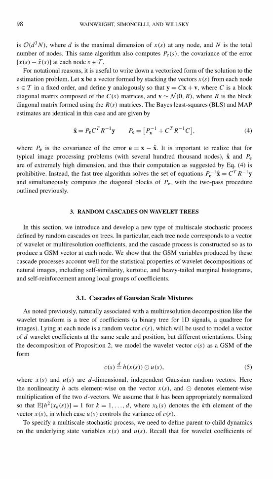
is O(d3N), where d is the maximal dimension of x(s) at any node, and N is the totalnumber of nodes. This same algorithm also computes Pe(s), the covariance of the error[x(s)− x(s)] at each node s ∈ T .
For notational reasons, it is useful to write down a vectorized form of the solution to theestimation problem. Let x be a vector formed by stacking the vectors x(s) from each nodes ∈ T in a fixed order, and define y analogously so that y = Cx + v, where C is a blockdiagonal matrix composed of the C(s) matrices, and v ∼ N (0,R), where R is the blockdiagonal matrix formed using the R(s) matrices. The Bayes least-squares (BLS) and MAPestimates are identical in this case and are given by
x = PeCT R−1y Pe = [
P−1x +CT R−1C
], (4)
where Pe is the covariance of the error e = x − x. It is important to realize that fortypical image processing problems (with several hundred thousand nodes), x and Pe
are of extremely high dimension, and thus their computation as suggested by Eq. (4) isprohibitive. Instead, the fast tree algorithm solves the set of equations P−1
e x = CT R−1yand simultaneously computes the diagonal blocks of Pe, with the two-pass procedureoutlined previously.
3. RANDOM CASCADES ON WAVELET TREES
In this section, we introduce and develop a new type of multiscale stochastic processdefined by random cascades on trees. In particular, each tree node corresponds to a vectorof wavelet or multiresolution coefficients, and the cascade process is constructed so as toproduce a GSM vector at each node. We show that the GSM variables produced by thesecascade processes account well for the statistical properties of wavelet decompositions ofnatural images, including self-similarity, kurtotic, and heavy-tailed marginal histograms,and self-reinforcement among local groups of coefficients.
3.1. Cascades of Gaussian Scale Mixtures
As noted previously, naturally associated with a multiresolution decomposition like thewavelet transform is a tree of coefficients (a binary tree for 1D signals, a quadtree forimages). Lying at each node is a random vector c(s), which will be used to model a vectorof d wavelet coefficients at the same scale and position, but different orientations. Usingthe decomposition of Proposition 2, we model the wavelet vector c(s) as a GSM of theform
c(s)d= h(x(s))� u(s), (5)
where x(s) and u(s) are d-dimensional, independent Gaussian random vectors. Herethe nonlinearity h acts element-wise on the vector x(s), and � denotes element-wisemultiplication of the two d-vectors. We assume that h has been appropriately normalizedso that E[h2(xk(s))] = 1 for k = 1, . . . , d , where xk(s) denotes the kth element of thevector x(s), in which case u(s) controls the variance of c(s).
To specify a multiscale stochastic process, we need to define parent-to-child dynamicson the underlying state variables x(s) and u(s). Recall that for wavelet coefficients of
RANDOM CASCADES ON WAVELET TREES 99
natural images, the parent and child vectors are close to decorrelated. We can express thecovariance between c(s) and its parent c(sγ ) as
cov[c(s), c(sγ )] = E{h(x(s))[h(x(sγ ))]T } � cov[u(s), u(sγ )],
where we have used the independence of x and u. This relationship shows that thedecorrelation of c(s) and c(sγ ) is determined by the u process. Therefore, to model waveletcoefficients of natural images, it is appropriate to choose u(s) as a white noise process onthe tree T , uncorrelated from node to node. In contrast, the vector x(s) must depend onits parent x(sγ ), in order to capture the strong property of local reinforcement in waveletcoefficients of natural images. Therefore, the GSM representation of Eq. (5) decomposesthe wavelet vector c(s) into two random components, one of which controls the correlationstructure, while the other controls reinforcement among wavelet coefficients.
We model the white noise process u(s) as
u(s)=D(s)ζ(s), ζ(s)∼N (0, I ), (6)
so that D(s) controls any scale-to-scale variation (and hence the scaling law) for theprocess. To capture the dependency in the premultiplier process x(s), we use a MAR model
x(s)=Ax(sγ )+Bw(s), (7)
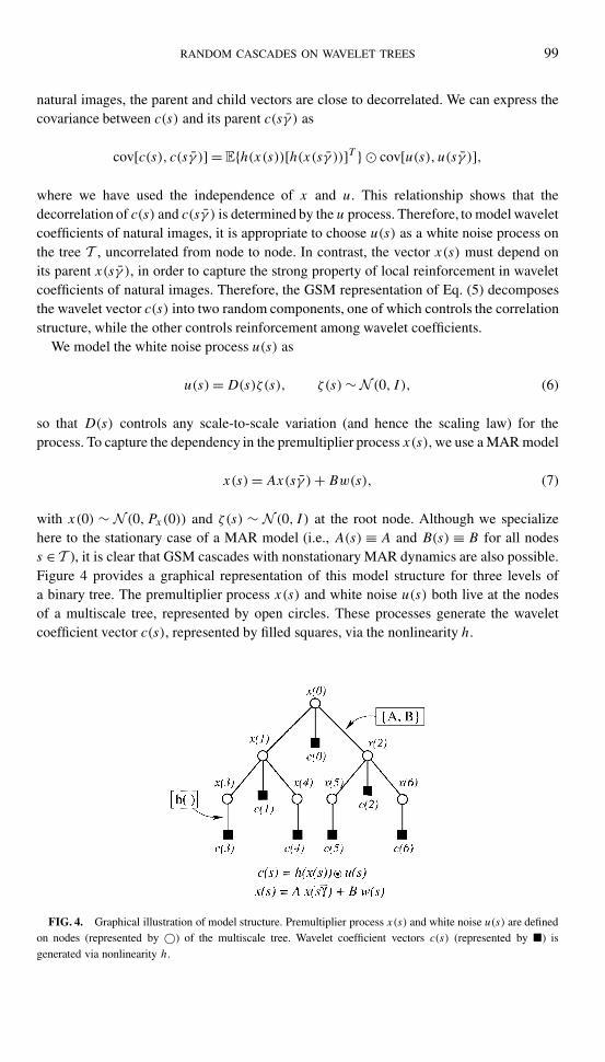
with x(0) ∼ N (0,Px(0)) and ζ(s) ∼ N (0, I ) at the root node. Although we specializehere to the stationary case of a MAR model (i.e., A(s) ≡ A and B(s) ≡ B for all nodess ∈ T ), it is clear that GSM cascades with nonstationary MAR dynamics are also possible.Figure 4 provides a graphical representation of this model structure for three levels ofa binary tree. The premultiplier process x(s) and white noise u(s) both live at the nodesof a multiscale tree, represented by open circles. These processes generate the waveletcoefficient vector c(s), represented by filled squares, via the nonlinearity h.
FIG. 4. Graphical illustration of model structure. Premultiplier process x(s) and white noise u(s) are definedon nodes (represented by ©) of the multiscale tree. Wavelet coefficient vectors c(s) (represented by �) isgenerated via nonlinearity h.
100 WAINWRIGHT, SIMONCELLI, AND WILLSKY
Equations (5), (6), and (7) together specify the coefficients c(s) of a multiresolutiondecomposition on a tree. For each node s, let m(s) be its spatial scale, and let p(s) beits spatial location in the image plane. The quantity c(s) is a random vector of waveletcoefficients for a set of different orientations at the same spatial location. For the 1Dexamples shown subsequently, we use an orthonormal wavelet representation, whereasfor 2D applications to images, we use the steerable pyramid [51], an overcompleterepresentation that divides the image into subbands localized in both scale and orientation.A steerable pyramid can be designed with any number of orientation bands; for the workreported here, we use d = 4 orientations. These coefficients then define a random imagevia the inverse transform
I(p1,p2)=∑s∈T
d∑k=1
ci(s)ψk;s (p1,p2), (8)
where (p1,p2) is a point in the 2D image plane, ck(s) is the kth element of c(s)(corresponding to the kth orientation), and ψk;s corresponds to the multiresolution basiselement corresponding to orientation k, and centered at scale and position (m(s),p(s)).
An advantage of the steerable pyramid for image processing tasks (e.g., denoising) is itstranslation invariance [51]. Achieving this invariance requires overcompleteness, implyingthat there is redundancy in each vector of coefficients c(s). In principle, this can be easilyaccommodated by taking ζ(s) in (6) to be a lower dimensional random vector, so thatD(s) is rectangular. For the work reported here, we have taken ζ(s) to be of the samedimension as u(s) and hence c(s). This is not a strictly accurate model since it suggeststhat there are more degrees of freedom in the c(s) than there should be; however, we havefound this formulation to be adequate in practice.
3.2. Properties of GSM Cascades
In this section, we examine the properties of random cascades of Gaussian scalemixtures on trees. We show that they are well-suited to capturing the statistical behavior ofmultiresolution coefficients from natural images.
3.2.1. Self-Similarity
Recall that self-similarity of a process means that its statistics are invariant (up toa multiplicative constant) under any change of scale. Note that GSM tree processes, asdefined above, are generated by a discrete multiresolution transform as in Eq. (8). Suchprocesses can never be strictly self-similar. However, by appropriate choice of parameters,we can ensure that they satisfy a weaker form of self-similarity, known as dyadic self-similarity. In particular, dyadic self-similarity of the random image I(p1,p2) means that
I(p1,p2)d= 2−kγ I(2k(p1,p2)) for all integers k, where γ is a parameter. From Eq. (8), it
can be shown that the synthesized process I(t) will be dyadically self-similar if and only if
the basis coefficients satisfy c(s)d= 2γ [m(t)−m(s)]c(t) for all nodes s, t ∈ T . We guarantee
this condition by choosing D(s) = 2−γm(s) in Eq. (6) and taking the state process x(s) to
be stationary, so that x(s)d= x(t) for all nodes s, t ∈ T . The parameter γ > 0 controls the
drop-off in the power spectrum of the synthesized process (e.g., [12]).
RANDOM CASCADES ON WAVELET TREES 101
3.2.2. Marginal Distributions
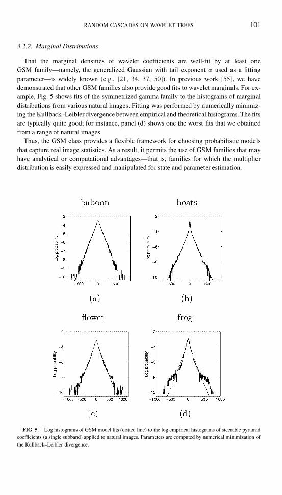
That the marginal densities of wavelet coefficients are well-fit by at least oneGSM family—namely, the generalized Gaussian with tail exponent α used as a fittingparameter—is widely known (e.g., [21, 34, 37, 50]). In previous work [55], we havedemonstrated that other GSM families also provide good fits to wavelet marginals. For ex-ample, Fig. 5 shows fits of the symmetrized gamma family to the histograms of marginaldistributions from various natural images. Fitting was performed by numerically minimiz-ing the Kullback–Leibler divergence between empirical and theoretical histograms. The fitsare typically quite good; for instance, panel (d) shows one the worst fits that we obtainedfrom a range of natural images.
Thus, the GSM class provides a flexible framework for choosing probabilistic modelsthat capture real image statistics. As a result, it permits the use of GSM families that mayhave analytical or computational advantages—that is, families for which the multiplierdistribution is easily expressed and manipulated for state and parameter estimation.
FIG. 5. Log histograms of GSM model fits (dotted line) to the log empirical histograms of steerable pyramidcoefficients (a single subband) applied to natural images. Parameters are computed by numerical minimization ofthe Kullback–Leibler divergence.
102 WAINWRIGHT, SIMONCELLI, AND WILLSKY
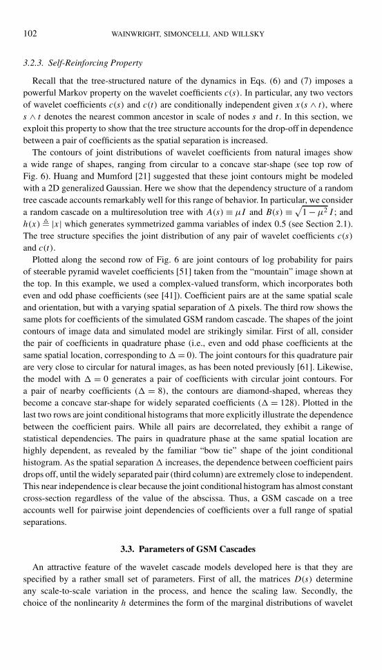
3.2.3. Self-Reinforcing Property
Recall that the tree-structured nature of the dynamics in Eqs. (6) and (7) imposes apowerful Markov property on the wavelet coefficients c(s). In particular, any two vectorsof wavelet coefficients c(s) and c(t) are conditionally independent given x(s ∧ t), wheres ∧ t denotes the nearest common ancestor in scale of nodes s and t . In this section, weexploit this property to show that the tree structure accounts for the drop-off in dependencebetween a pair of coefficients as the spatial separation is increased.
The contours of joint distributions of wavelet coefficients from natural images showa wide range of shapes, ranging from circular to a concave star-shape (see top row ofFig. 6). Huang and Mumford [21] suggested that these joint contours might be modeledwith a 2D generalized Gaussian. Here we show that the dependency structure of a randomtree cascade accounts remarkably well for this range of behavior. In particular, we considera random cascade on a multiresolution tree with A(s) ≡ µI and B(s) ≡ √
1 −µ2 I ; andh(x)� |x| which generates symmetrized gamma variables of index 0.5 (see Section 2.1).The tree structure specifies the joint distribution of any pair of wavelet coefficients c(s)and c(t).
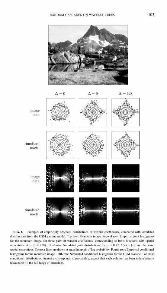
Plotted along the second row of Fig. 6 are joint contours of log probability for pairsof steerable pyramid wavelet coefficients [51] taken from the “mountain” image shown atthe top. In this example, we used a complex-valued transform, which incorporates botheven and odd phase coefficients (see [41]). Coefficient pairs are at the same spatial scaleand orientation, but with a varying spatial separation of 5 pixels. The third row shows thesame plots for coefficients of the simulated GSM random cascade. The shapes of the jointcontours of image data and simulated model are strikingly similar. First of all, considerthe pair of coefficients in quadrature phase (i.e., even and odd phase coefficients at thesame spatial location, corresponding to 5= 0). The joint contours for this quadrature pairare very close to circular for natural images, as has been noted previously [61]. Likewise,the model with 5 = 0 generates a pair of coefficients with circular joint contours. Fora pair of nearby coefficients (5 = 8), the contours are diamond-shaped, whereas theybecome a concave star-shape for widely separated coefficients (5 = 128). Plotted in thelast two rows are joint conditional histograms that more explicitly illustrate the dependencebetween the coefficient pairs. While all pairs are decorrelated, they exhibit a range ofstatistical dependencies. The pairs in quadrature phase at the same spatial location arehighly dependent, as revealed by the familiar “bow tie” shape of the joint conditionalhistogram. As the spatial separation5 increases, the dependence between coefficient pairsdrops off, until the widely separated pair (third column) are extremely close to independent.This near independence is clear because the joint conditional histogram has almost constantcross-section regardless of the value of the abscissa. Thus, a GSM cascade on a treeaccounts well for pairwise joint dependencies of coefficients over a full range of spatialseparations.
3.3. Parameters of GSM Cascades
An attractive feature of the wavelet cascade models developed here is that they arespecified by a rather small set of parameters. First of all, the matrices D(s) determineany scale-to-scale variation in the process, and hence the scaling law. Secondly, thechoice of the nonlinearity h determines the form of the marginal distributions of wavelet
RANDOM CASCADES ON WAVELET TREES 103
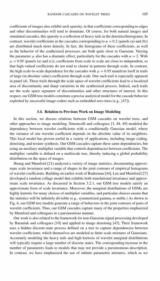
FIG. 6. Examples of empirically observed distributions of wavelet coefficients, compared with simulateddistributions from the GSM gamma model. Top row: Mountain image. Second row: Empirical joint histogramsfor the mountain image, for three pairs of wavelet coefficients, corresponding to basis functions with spatialseparations 5 = {0,8,128}. Third row: Simulated joint distributions for µ = 0.92, h(x) = |x|, and the samespatial separations. Contour lines are drawn at equal intervals of log probability. Fourth row: Empirical conditionalhistograms for the mountain image. Fifth row: Simulated conditional histograms for the GSM cascade. For theseconditional distributions, intensity corresponds to probability, except that each column has been independentlyrescaled to fill the full range of intensities.
104 WAINWRIGHT, SIMONCELLI, AND WILLSKY
coefficients, including tail behavior and kurtosis. Thirdly, the system matrices A determinethe dependency of the underlying premultiplier process x(s) from node to node.
Variations in D(s) control the amount of power at high frequencies relative tolow frequencies, and hence the overall smoothness of the process. The effect of suchchanges is well-understood from studies of f−γ type Gaussian processes on multiscaletrees (e.g., [12, 60]). Here we investigate the effect of varying the nonlinearity h, as well asthe system matrices. In particular, we simulate a one-dimensional cascade (i.e., the waveletrepresentation of a 1D process) with the parameters D(s) = 2−γm(s) and γ = 1.5; thenonlinearity h(x) = (x+)α ; and system matrices A = µ; and B = √
1 −µ2, where thechoices of the parameter α and the scale-to-scale dependence µ were varied.
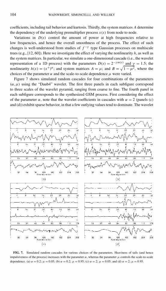
Figure 7 shows simulated random cascades for four combinations of the parameters(α,µ) using the “Daub4” wavelet. The first three panels in each subfigure correspondto three scales of the wavelet pyramid, ranging from coarse to fine. The fourth panel ineach subfigure corresponds to the synthesized GSM process. First considering the effectof the parameter α, note that the wavelet coefficients in cascades with α = 2 (panels (c)and (d)) exhibit sparse behavior, in that a few outlying values tend to dominate. The wavelet
FIG. 7. Simulated random cascades for various choices of the parameters. Heaviness of tails (and henceimpulsiveness of the process) increases with the parameter α, whereas the parameter µ controls the scale-to-scaledependence. (a) α = 0.2; µ= 0.05; (b) α = 0.2; µ= 0.95; (c) α = 2; µ= 0.05; and (d) α = 2; µ= 0.95.
RANDOM CASCADES ON WAVELET TREES 105
coefficients of images also exhibit such sparsity, in that coefficients corresponding to edgesand other discontinuities will tend to dominate. Of course, for both natural images andsimulated cascades, this sparsity is a reflection of heavy tails in the densities/histograms. Incontrast, wavelet coefficients in the cascades corresponding to α = 0.2 (panels (a) and (b))are distributed much more densely. In fact, the histograms of these coefficients, as wellas the behavior of the synthesized processes, are both quite close to Gaussian. Varyingthe parameter µ also has a dramatic effect, particularly for the cascades with α = 2. Withµ= 0.05 (panels (a) and (c)), coefficients from scale to scale are close to independent, sothat high-valued coefficients do not tend to cluster in patterns through scale. In contrast,the high scale-to-scale dependence for the cascades with µ= 0.95 manifests itself in trailsof large (in absolute value) coefficients through scale. One such trail is especially apparentin panel (d). These trails through the scale space of wavelet coefficients lead to a localizedarea of discontinuity and sharp variations in the synthesized process. Indeed, such trailsare the scale space signature of discontinuities and other structures of interest. In thisrespect, our GSM tree models constitute a precise analytical model for the cascade behaviorexploited by successful image coders such as embedded zero-trees (e.g., [47]).
3.4. Relation to Previous Work on Image Modeling
In this section, we discuss relations between GSM cascades on wavelet trees, andother approaches to image modeling. Simoncelli and colleagues [3, 48, 49] modeled thedependency between wavelet coefficients with a conditionally Gaussian model, wherethe variance of one wavelet coefficient depends on the absolute value of its neighbors.This local model has proven useful in a variety of applications, including image coding,denoising, and texture synthesis. Our GSM cascades capture these same dependencies, butusing an auxiliary multiplier variable that controls dependencies between coefficients. Themultiplier variable is defined on a multiscale tree, thereby inducing a global probabilitydistribution on the space of images.
Huang and Mumford [21] analyzed a variety of image statistics, documenting approxi-mate scale invariance and a range of shapes in the joint contours of empirical histogramsof wavelet coefficients. Building on earlier work of Ruderman [44], Lee and Mumford [27]developed a random collage model that exhibits both translational invariance and approx-imate scale invariance. As discussed in Section 3.2.1, our GSM tree models satisfy anapproximate form of scale invariance. Moreover, the marginal distributions of GSMs arehighly kurtotic for many choices of multiplier variables, and particular choices ensure thatthe statistics will be infinitely divisible (e.g., symmetrized gamma, α-stable.) As shown inFig. 6, our GSM tree models generate a range of behaviors in the joint contours of pairs ofwavelet coefficients. Thus, our GSM cascades capture many of the properties emphasizedby Mumford and colleagues in a parsimonious manner.
Our work is also related to the framework for non-Gaussian signal processing developedby Baraniuk and colleagues [10] and applied to image denoising [43]. Their frameworkuses a hidden discrete-state process defined on a tree to capture dependencies betweenwavelet coefficients, which themselves are modeled as finite scale mixtures of Gaussians.Accurately modeling the heavy tails and high kurtosis of wavelet marginal distributionswill typically require a large number of discrete states. The corresponding increase in thenumber of parameters leads to models that may not provide a parsimonious description.In contrast, we have emphasized the use of infinite parametric mixtures, which as we
106 WAINWRIGHT, SIMONCELLI, AND WILLSKY
have shown, accurately capture both the heavy tails and high kurtosis of wavelet marginaldistributions with a small number of parameters.
4. ESTIMATION
We now turn to problems of estimation in GSM cascades on wavelet trees. Suchproblems involve using data or observations to make inferences either about the state(i.e., x(s) and u(s)) of the GSM or about unknown model parameters. Of particular interestare estimates of the premultiplier process x(s), which determine the multiplier h(x(s)).A significant benefit of the GSM framework is that conditioned on knowledge of thepremultiplier, a GSM model reduces to a linear-Gaussian system, which can be analyzedby standard techniques. In the context of image processing, estimates of the premultiplierare of potential use for a variety of applications (e.g., coding and denoising).
In this section, we develop a Newton-like algorithm for MAP estimation of thepremultiplier x(s) based on noisy observations. The cost of computing intermediatequantities within each iteration scales linearly in problem size, because very fast algorithms(see Section 2.2) can be applied to the underlying Gaussian-tree structure. Furthermore,under suitable regularity conditions, this algorithm has a number of desirable properties,including guaranteed convergence to a local optimum at a quadratic rate. We then showhow this algorithm can be used as the basis of a method for wavelet domain denoising. Nextwe turn to the problem of estimating parameters that specify a GSM model and developa technique in which state estimates are exploited in intermediate computations. Theresultant technique is an approximate form of expectation-maximization algorithm [14],where intermediate computation is again efficient due to the tree structure.
4.1. State Estimation
Here we consider the problem of estimating the premultiplier x(s) given noisyobservations
y(s)= h(x(s))� u(s)+ v(s), (9)
where v(s) ∼ N (0,R(s)) is observation noise. An interesting feature of this problemis that unlike the standard linear observation problem (see Section 2.2)), the task ofestimating x(s) given noiseless observations (i.e., R(s) ≡ 0) is not trivial. Indeed, evenin the absence of v(s), the state u(s) effectively acts as a multiplicative form of noise. Withthe noise v(s) present, we have an estimation problem that is nonlinear and includes bothadditive and multiplicative noise terms.
Given that we have a dynamical system defined on a tree, optimal estimation can, inprinciple, be performed by a two-pass algorithm, sweeping up and down the tree. Forthe linear-Gaussian case described in Section 2.2, computation of the optimal estimate(which is simultaneously the BLS and MAP estimate) is particularly simple, involving thepassing of conditional means and covariances only. In general, for nonlinear/non-Gaussianproblems, however, not only are the BLS and MAP estimates different, but neither is easyto compute. However, the GSM models developed here have structure that can be exploitedto produce an efficient and conceptually interesting algorithm for MAP estimation.
To set up the estimation problem, let x denote a vector formed by concatenatingthe state vectors x(s) at each node, and define the vector y similarly. Recall that the
RANDOM CASCADES ON WAVELET TREES 107
computation of the MAP estimate involves the solution of the optimization problemxMAP � arg minx[− logp(x|y)]. Hereafter we simply write x to mean this MAP estimate.At a global level, our algorithm is a Newton-type method applied to the objective functionf (x) � − logp(x|y). That is, it entails generating a sequence {xn} via the recursionxn+1 = xn + αnS−1(xn)∇f (xn), where the matrix S(xn) is the Hessian of f , or somesuitable approximation to it; and αn is a step-size parameter. This class of methods isattractive (see [2]), because under suitable regularity conditions, not only is convergence toa local minimum guaranteed, but also the convergence rate is quadratic. The disadvantageof such methods, in general, is that the computation of the descent direction dn �−S−1(xn)∇f (xn) may be extremely costly. This concern is especially valid in imageprocessing applications, where the dimension of the matrix S(xn) will be of the order 105
or higher.One of the most important features of our model set-up is that the computation required
for each step of the Newton recursion can indeed be performed efficiently. More precisely,the computation of the descent direction is equivalent to the solution of a linear MARestimation problem, allowing the efficient algorithm of [8] described in Section 2.2 to beused for its computation. In order to demonstrate this equivalence, we rewrite the objectivefunction as f (x)= − logp(y|x)− logp(x)+ C using Bayes’ rule, where C is a constantthat absorbs terms not depending on x. The vector x is distributed as N (0,Px), where thelarge covariance matrix Px is defined by the system matrices A and B in Eq. (7). As aresult, the log prior term can be written as 1
2 xT P−1x x + C. Finally, since the data y(s) at
each node is conditionally independent of all other data given the state vector x, we canwrite
f (x)= −N∑s=1
logp(y(s)|x(s))+ 1
2xT P−1
x x +C.
From this representation of f , it can be seen that the Hessian of f will have theform ∇2f (x) = P−1
x + D(x), where D(x) is a block diagonal matrix, with each blockcorresponding to a node s. With this form of the Hessian, the descent direction dn isgiven by dn = −[P−1
x +D(xn)]−1∇f (xn). Comparing this form of the descent directionto the linear-Gaussian problem given in Eq. (4), it is clear that the two problems areequivalent with appropriate identification of data terms, observation matrix, and noisecovariance. Further details of these identifications, as well as calculation of the Hessian,the gradient ∇f (x), and D(x) can be found in Appendix B.
Note that the overall structure of this MAP estimation algorithm is of a hybrid form.The Newton-like component involves an approximation of the objective function f thatis performed globally on the entire graph at once. Local graphical structure is exploitedwithin each iteration where the descent direction is computed by extremely efficient anddirect algorithms for linear multiscale tree problems [8]. Thus, the complexity per iterationscales as O(d3N), where N is the number of nodes, and d is the number of orientations.As a Newton method, quadratic convergence is guaranteed for suitably smooth choicesof the nonlinearity. This method is distinct from extended Kalman filtering (e.g., [24]),a technique for approximate estimation of nonlinear dynamic systems, because theobjective function is approximated globally on the entire state trajectory at once.
Another important characteristic of the GSM framework is that conditioning on thepremultiplier x(s) reduces the model to the linear-Gaussian case. That is, when the
108 WAINWRIGHT, SIMONCELLI, AND WILLSKY
multiplier is known, the observations (9) are of the standard linear-Gaussian form.If, indeed x(s) were known exactly, we would have that Pc(s) = H [x(s)]Pu(s)H [x(s)],where Pu(s) = D(s)DT (s) is the covariance of u(s), and the matrix H [x(s)] �diag {h(x(s))}. This suggests a suboptimal estimate in which we replace x(s) by x(s),namely
c(s)= Pc(s)[Pc(s)+R(s)
]−1y(s), (10)
where Pc(s) = H [x(s)]Pu(s)H [x(s)]. It is this form of wavelet estimator that we use inour application to image denoising in Section 5.
4.2. Relation to Other Estimators
There are a number of interesting links between the GSM tree estimator, developedhere, and previous approaches to wavelet denoising. In particular, there is a large classof pointwise approaches to denoising, so called because they operate independently oneach wavelet coefficient. The link to the GSM framework comes from the Bayesianperspective, in which many of these methods can be shown to be equivalent to MAP orBLS estimation under a particular kind of GSM prior to the marginal distribution. Forexample, soft shrinkage [15], a widely studied form of pointwise estimate, is equivalent toa MAP estimate with a certain GSM prior, namely, a Laplacian or generalized Gaussiandistribution with tail exponent α = 1 (see [4]). Specifically, suppose that the prior on xhas the form px(x) ∝ exp(−(λ/2)|x|) and that y is an observation of x contaminated byGaussian noise of variance σ 2. Under these assumptions, it is straightforward to verify thatthe MAP estimate is given by
xMAP = [y − sign(y − τ )τ ]+, (11)
where τ � λσ 2/2. For the purposes of comparison, we apply this type of soft thresholdingto image denoising in Section 5. Additional relations between thresholding and MAPestimators are discussed in [37]. It is shown in [50] that by varying the tail parameter αof a generalized Gaussian prior, it is possible to derive a full family of pointwise Bayesleast-squares estimators.
The GSM framework can also be related to the James–Stein estimator (JSE), a techniquewith an interesting and often controversial history. The JSE applies to the problem ofestimating the fixed mean c of a multivariate normal distribution from noisy observationsy = c+v, where v ∼N (0, σ 2I) and the length of the vector quantities is p. The maximumlikelihood estimate of c, which is simply the data y itself, was long thought to be best inthe sense that no other estimator could achieve a lower mean-squared error (MSE) for allvalues of c. However, in 1961 James and Stein [23] introduced an estimator of the mean fordimension p ≥ 3 that achieves a uniformly lower MSE for all values of c. The empiricalBayesian derivation for the JSE (see, e.g., [16]) provides the link to GSMs. In theempirical Bayes formulation, c is modeled as a random quantity, distributed according toN (0, τ 2). If the quantity τ were known, then the Bayes least-squares estimate (BLSE) ofc given y would be given by cBLS = [(τ 2)/(τ 2 + σ 2)]y . For τ unknown, we can imaginetrying to mimic the BLSE by estimating τ 2, and then substituting this estimate into theformula for the BLSE. In fact, the JSE proceeds more directly by estimating the quantityσ 2/[τ 2 + σ 2] as (p − 2)σ 2/‖y‖2, which can be shown [26] to be an unbiased estimate.
RANDOM CASCADES ON WAVELET TREES 109
Substituting this estimate into the BLSE formula yields the positive-part JSE, defined asc= ([‖y‖2 − (p− 2)σ 2]+]/‖y‖2)y .
The link to Gaussian scale mixtures is clear. Under the empirical Bayesian interpretation,the JSE decomposes the unknown mean c into two parts c = τu, where u∼ N (0, I ), andτ is an unknown but fixed quantity. That is, the JSE decomposes the mean into a type ofGaussian scale mixture, involving a Gaussian component u and an unknown multiplier τ .For the Gaussian scale mixtures discussed in this paper, we typically viewed τ as a randomvariable and assigned it a prior under which we computed the MAP estimate. The JSE isvery similar, except that it does not assign a prior to τ , and it performs an operation thatis very close to ML estimation of σ 2/[τ 2 + σ 2]. Finally, both the JSE and the GSM treemethod replace the variance in standard linear-Gaussian equations (e.g., in Eq. (10)) by anestimated variance.
Although not always explicitly stated, many other approaches to image denoisingand image coding rely on a GSM-type decomposition. The roots of this approach liein the image coding literature, where researchers in the 1970s proposed dividing DCTcoefficients into groups according to their variance [6]. Similarly, Lee [28] proposedan enhancement technique that used local variances in the pixel domain, which is nowimplemented in the MATLAB wiener2 routine. More recent approaches also involvemodeling wavelet coefficients as scale mixture distributions (e.g., [5, 9, 29, 30, 35, 36, 52]).Another approach is to model dependency between the variance of a subband coefficientand its neighbors directly, using a conditionally Gaussian model [3, 48, 49]. Some modelspermit the variance parameter to assume only a discrete set of values (e.g., [29]), whereasothers allow a continuum of values. The latter models effectively correspond to infinitemixture models, similar to those emphasized in the current paper.
A step common to all these techniques, whether for denoising or coding, is to estimatethe multiplier or variance. Conditioned on the variance estimate, coefficients can bedenoised by the standard LLS estimator in Eq. (10). Many approaches use a maximumlikelihood (ML)-like estimate for the variance parameter, based on a local neighborhoodof coefficients. In such a ML framework, the variance parameter is viewed as an unknownbut fixed quantity, without a prior distribution. These forms of estimator are thus veryclose to the James–Stein estimator discussed previously. More recently, Mihcak et al. [36]assumed an exponential distribution on the variance parameter and performed a local andapproximate form of MAP estimation. This corresponds to a local GSM model using asymmetrized gamma distribution with parameter α = 1. Overall, the GSM tree frameworkpresented in this paper represents an extension from local to global models. Our modelsallow an arbitrary choice of the prior on the multiplier, which is controlled by the choice ofthe nonlinearity h. Moreover, the GSM tree algorithm computes the MAP estimate basedon a global prior model on the full multiresolution representation. This global prior, whichincorporates the strong self-reinforcing properties among wavelet coefficients, is inducedby the multiscale tree structure.
In the context of the underlying tree, our GSM cascade models are closely related tothe non-Gaussian modeling framework of Baraniuk and colleagues [10]. In their models,a multiscale, discrete-state multiplier process defined on a tree controls the dependencyamong wavelet coefficients, which are modeled as finite scale mixtures of Gaussians. Suchmodels have proven useful in various applications, including image denoising [43]. Forfinite mixtures in which the multiplier variable takes on discrete values, there exist direct
110 WAINWRIGHT, SIMONCELLI, AND WILLSKY
recursive algorithms for computing the marginal distributions of the discrete multiplierstates conditioned on the data. The BLS estimate of wavelet coefficients given noisyobservations can be obtained by taking expectations over these marginal distributions(see [10]). However, the computational complexity of computing marginal distributionsscales exponentially as ∼Md , where M is the number of multiplier states and d is thedimension of the multiplier. In practice, therefore, both the number of states and dimensionof the multiplier may be limited; for example, the denoising algorithm of [43] uses a lowand high variance state (M = 2) and a scalar multiplier at each node (d = 1). A smallnumber of multiplier states means that the models may not properly capture the non-Gaussian tail behavior and high kurtosis of wavelet marginals, whereas a low multiplierdimension will restrict the modeling of dependencies between orientations. In contrast,our GSM modeling framework emphasizes infinite scale mixtures of Gaussians. As wehave illustrated, these infinite mixtures accurately capture the non-Gaussian tail behaviorand high kurtosis of wavelet coefficients. Regardless of the particular GSM used, thecomplexity of our algorithm scales as ∼d3, where d is the dimension of multiplier vectorat each node.
4.3. Parameter Estimation
We now address the problem of estimating the parameters of a GSM random cascademodel. Recall that a GSM model is specified by a small set of quantities, namely, thematrices D(s) that control the scaling law; the pointwise nonlinearity h; and the systemmatrices A and B that control the MAR dynamics. Determining the matrices D(s)amounts to estimating the variance, and hence can be done with standard methods. Thenonlinearity h controls the marginal distributions, so that estimating h is similar to fittinga parameterized distribution to the marginal histograms of wavelet coefficients, again afairly standard procedure. The novel aspect of our GSM models are the system matrices Aand B that control the scale-to-scale dependence of the underlying premultiplier process,and it is on the estimation of these quantities that we focus here. In particular, let θ bea vector of parameters that specify these system matrices, so that we write the stationaryMAR dynamics as
x(s)=A(θ)x(sγ )+B(θ)w(s). (12)
The task is to estimate the parameter vector θ on the basis of noisy observations givenby Eq. (9).
We begin by observing that this set-up shares a characteristic common to many parame-ter estimation problems: namely, the estimation of θ would be relatively straightforwardgiven the premultiplier x. Given this property, the parameter estimation problem lendsitself to the use of the expectation-maximization (EM) algorithm [14], a technique fre-quently used to obtain the ML estimate of θ . Recall that the ML estimate is given byθML = arg maxθ∈;[logp(y; θ)], where; is the domain of θ . In accordance with its name,the EM algorithm alternates between taking expectations over a set of “hidden” variables xand then performing maximization of the resulting function. In particular, the E-step ofiteration n involves taking the expectation of the augmented log likelihood logp(x,y; θ)with respect to the conditional density p(x|y; θn−1), where θn−1 is the parameter estimatefrom the previous iteration. In the standard version of the EM algorithm, the M-step entailsfinding the global maximum of the resulting function. However, there exist other versions
RANDOM CASCADES ON WAVELET TREES 111
of EM (often called GEM for generalized EM [14]) in which the M-step consists of takinggradient step.
A disadvantage of EM-type algorithms is that calculating the expectation over theconditional density p(x|y; θn−1) can be difficult. This problem is often encountered forcontinuous-valued variables, where the integrals are typically intractable. One approachin such cases is to develop an approximation q(x|y; θn−1)≈ p(x|y; θn−1) and perform anapproximate E-step by taking expectations with respect to the distribution q , whose formis chosen to make such expectations comparatively easy to compute. It can be shown thatsuch approximate methods will still converge, although they need not converge to a localmaximum of the log likelihood, but rather to a local maximum of a lower bound on thelikelihood [25].
We have developed such an approximate EM method for parameter estimation in GSMsystems, where the approximation q to the conditional density is obtained from thealgorithm described in Section 4.1. It should be noted that even with an approximate formof the density, taking the expectation is not, in general, a straightforward task. Again theproblem stems from the high dimensionality of the conditional density—in applicationssuch as image processing, it will be on the order of 105 or 106. Nonetheless, we havefound that the tree structure of the problem can again be exploited to great advantage. Inparticular, we make use of highly efficient algorithms for Gaussian likelihood calculationon multiscale trees in order to perform gradient ascent. 6 This approximate EM algorithmitself is developed in Appendix C. Thus, by exploiting the tree structure, we obtain atractable technique for estimating the parameters specifying the system matrices.
5. ILLUSTRATIVE RESULTS
In this section, we present some illustrative results of the state estimation algorithmdeveloped in the previous section. We focus, in particular, on the problem estimatingwavelet coefficients c(s) on the basis of noisy observations y(s). The wavelet coefficientsare generated by GSM tree dynamics, and hence lie at the nodes of a multiresolution tree.However, to illustrate the basic properties of our estimator, we first consider its applicationto the estimation of 1D sequence of scalar-valued coefficients c(s) from a correspondingsequence of measurements. These sequences can be thought of as the successive values ofone of the components of c(s) and y(s) on a single coarse-to-fine path in a tree, such asthat in Fig. 3. Following this 1D example, we illustrate the application of our full algorithmto perform image denoising on a multiresolution quadtree of coefficients.
5.1. Examples in 1D
We first consider a scalar GSM process obtained by sampling a GSM tree processalong the unique tree path beginning at the root node and moving down the tree (fromparent to child), terminating at a specified fine-scale node. Such a sample path revealsthe scale-to-scale dependence inherent in a GSM tree process. We generate the processon the tree with dynamics of the form x(s) = µx(s − 1) + √
1 −µ2w(s) and c(s) =h(x(s))u(s), where u(s) and w(s) are distributed as N (0,1) at each node. We estimate
6 Thus, the overall procedure actually exploits tree structure twice: once to compute the density q(x|y, θn−1)
using the estimation algorithm of Section 4.1 and again in order to calculate the required expectation.
112 WAINWRIGHT, SIMONCELLI, AND WILLSKY
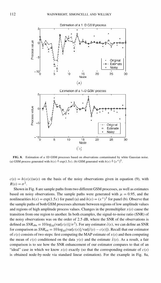
FIG. 8. Estimation of a 1D GSM processes based on observations contaminated by white Gaussian noise.(a) GSM process generated with h(x)� exp(1.5x). (b) GSM generated with h(x)� [x+]3.
c(s) = h(x(s))u(s) on the basis of the noisy observations given in equation (9), withR(s)= σ 2.
Shown in Fig. 8 are sample paths from two different GSM processes, as well as estimatesbased on noisy observations. The sample paths were generated with µ = 0.95, and thenonlinearities h(x)= exp(1.5x) for panel (a) and h(x)= (x+)3 for panel (b). Observe thatthe sample paths of both GSM processes alternate between regions of low amplitude valuesand regions of high amplitude process values. Changes in the premultiplier x(s) cause thetransition from one region to another. In both examples, the signal-to-noise ratio (SNR) ofthe noisy observations was on the order of 2.5 dB, where the SNR of the observations isdefined as SNRobs = 10 log10(var[c(s)]/σ 2). For any estimator c(s), we can define an SNRfor comparison as SNRest = 10 log10(var[c(s)]/var[c(s)− c(s)]). Recall that our estimatorof c(s) consists of two steps: first computing the MAP estimate of x(s) and then computingthe mean of c(s) conditioned on the data y(s) and the estimate x(s). As a result, a faircomparison is to see how the SNR enhancement of our estimator compares to that of an“ideal” case in which we know x(s) exactly (so that the corresponding estimate of c(s)is obtained node-by-node via standard linear estimation). For the example in Fig. 8a,
RANDOM CASCADES ON WAVELET TREES 113
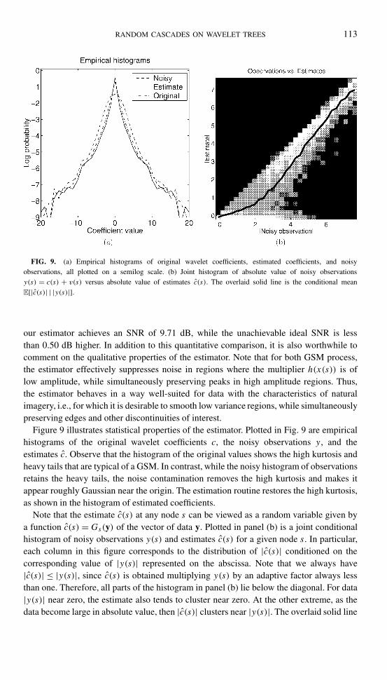
FIG. 9. (a) Empirical histograms of original wavelet coefficients, estimated coefficients, and noisyobservations, all plotted on a semilog scale. (b) Joint histogram of absolute value of noisy observationsy(s) = c(s) + v(s) versus absolute value of estimates c(s). The overlaid solid line is the conditional meanE[|c(s)| | |y(s)|].
our estimator achieves an SNR of 9.71 dB, while the unachievable ideal SNR is lessthan 0.50 dB higher. In addition to this quantitative comparison, it is also worthwhile tocomment on the qualitative properties of the estimator. Note that for both GSM process,the estimator effectively suppresses noise in regions where the multiplier h(x(s)) is oflow amplitude, while simultaneously preserving peaks in high amplitude regions. Thus,the estimator behaves in a way well-suited for data with the characteristics of naturalimagery, i.e., for which it is desirable to smooth low variance regions, while simultaneouslypreserving edges and other discontinuities of interest.
Figure 9 illustrates statistical properties of the estimator. Plotted in Fig. 9 are empiricalhistograms of the original wavelet coefficients c, the noisy observations y , and theestimates c. Observe that the histogram of the original values shows the high kurtosis andheavy tails that are typical of a GSM. In contrast, while the noisy histogram of observationsretains the heavy tails, the noise contamination removes the high kurtosis and makes itappear roughly Gaussian near the origin. The estimation routine restores the high kurtosis,as shown in the histogram of estimated coefficients.
Note that the estimate c(s) at any node s can be viewed as a random variable given bya function c(s) =Gs(y) of the vector of data y. Plotted in panel (b) is a joint conditionalhistogram of noisy observations y(s) and estimates c(s) for a given node s. In particular,each column in this figure corresponds to the distribution of |c(s)| conditioned on thecorresponding value of |y(s)| represented on the abscissa. Note that we always have|c(s)| ≤ |y(s)|, since c(s) is obtained multiplying y(s) by an adaptive factor always lessthan one. Therefore, all parts of the histogram in panel (b) lie below the diagonal. For data|y(s)| near zero, the estimate also tends to cluster near zero. At the other extreme, as thedata become large in absolute value, then |c(s)| clusters near |y(s)|. The overlaid solid line
114 WAINWRIGHT, SIMONCELLI, AND WILLSKY
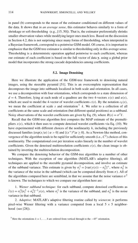
in panel (b) corresponds to the mean of the estimator conditioned on different values ofthe data. It shows that in an average sense, this estimator behaves similarly to a form ofshrinkage or soft thresholding (e.g., [15, 50]). That is, the estimator preferentially shrinkssmaller observation values while modifying larger ones much less. Based on the discussionin Section 4.2, this is not surprising since many forms of thresholding, when interpreted ina Bayesian framework, correspond to a pointwise GSM model. Of course, it is important toemphasize that the GSM tree estimator is similar to thresholding only in this average sense.Thresholding is a deterministic operation applied pointwise to each coefficient, whereasour estimate of each coefficient is based on the full vector of data y, using a global priormodel that incorporates the strong cascade dependencies among coefficients.
5.2. Image Denoising
Here we illustrate the application of the GSM-tree framework to denoising naturalimages, using the steerable pyramid [51]. This is an overcomplete representation thatdecomposes the image into subbands localized in both scale and orientation. In all cases,we use a decomposition with four orientations, which corresponds to a state dimension ofd = 4. Therefore, lying at each node of a quadtree are the two 4-vectors x(s) and u(s),which are used to model the 4-vector of wavelet coefficients c(s). By the notation ck(s),we mean the coefficient at scale s and orientation 7 k. We refer to a collection of allcoefficients at the same scale and orientation (but different spatial positions) as a subband.Noisy observations of the wavelet coefficients are given by Eq. (9), where R(s)= σ 2I .
Recall that the GSM-tree algorithm first computes the MAP estimate of the premulti-pliers x(s), which it then uses to compute denoised wavelet coefficients via Eq. (10). Wehave experimented with different choices of the nonlinearity h, including the previouslydiscussed families {exp(x/α) | α > 0} and {(x+)α|α ≥ 0}. As a Newton-like method, con-vergence of the algorithm tends to be rapid for sufficiently smooth (i.e., C2) choices of thisnonlinearity. The computational cost per iteration scales linearly in the number of waveletcoefficients. Given the denoised multiresolution coefficients c(s), the clean image is ob-tained by inverting the multiresolution decomposition.
We compare the denoising behavior of the GSM-tree algorithm to a number of othertechniques. With the exception of one algorithm (MATLAB’s adaptive filtering), alltechniques are applied to the steerable pyramid decomposition, and involve an estimateof the subband variance. This estimate is given by σ 2
c = [var(y(s))− σ 2n ]+, where σ 2
n isthe variance of the noise in the subband (which can be computed directly from σ ). All ofthe algorithms compared here are semiblind, in that we assume that the noise variance σ 2
is known. The techniques to which we compare our algorithm here are:
1. Wiener subband technique: for each subband, compute denoised coefficients asc(s)= σ 2
c [σ 2c + σ 2
n ]−1y(s), where σ 2c is the variance of the subband, and σ 2
n is the noisevariance in that subband.
2. Adaptive: MATLAB’s adaptive filtering routine called by wiener.m: it performspixel-wise Wiener filtering with a variance computed from a local 5 × 5 neighbor-hood (see [28]).
7 Here the orientations k = 1, . . . ,4 are ordered from vertical through to the −45◦ orientation.
RANDOM CASCADES ON WAVELET TREES 115
3. Soft thresholding: [15] For each subband, compute the soft threshold given inEq. (11), where the threshold t = λσ 2
n /2 is determined by the noise variance σ 2n and the
scale parameter λ of a Laplacian distribution fit to the subband marginal.
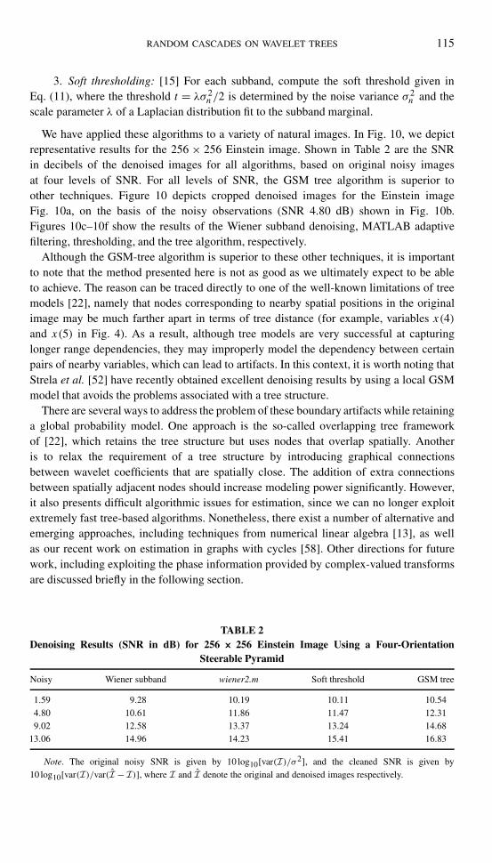
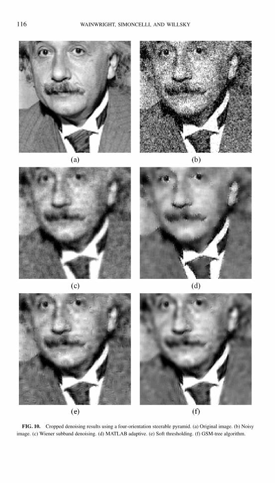
We have applied these algorithms to a variety of natural images. In Fig. 10, we depictrepresentative results for the 256 × 256 Einstein image. Shown in Table 2 are the SNRin decibels of the denoised images for all algorithms, based on original noisy imagesat four levels of SNR. For all levels of SNR, the GSM tree algorithm is superior toother techniques. Figure 10 depicts cropped denoised images for the Einstein imageFig. 10a, on the basis of the noisy observations (SNR 4.80 dB) shown in Fig. 10b.Figures 10c–10f show the results of the Wiener subband denoising, MATLAB adaptivefiltering, thresholding, and the tree algorithm, respectively.
Although the GSM-tree algorithm is superior to these other techniques, it is importantto note that the method presented here is not as good as we ultimately expect to be ableto achieve. The reason can be traced directly to one of the well-known limitations of treemodels [22], namely that nodes corresponding to nearby spatial positions in the originalimage may be much farther apart in terms of tree distance (for example, variables x(4)and x(5) in Fig. 4). As a result, although tree models are very successful at capturinglonger range dependencies, they may improperly model the dependency between certainpairs of nearby variables, which can lead to artifacts. In this context, it is worth noting thatStrela et al. [52] have recently obtained excellent denoising results by using a local GSMmodel that avoids the problems associated with a tree structure.
There are several ways to address the problem of these boundary artifacts while retaininga global probability model. One approach is the so-called overlapping tree frameworkof [22], which retains the tree structure but uses nodes that overlap spatially. Anotheris to relax the requirement of a tree structure by introducing graphical connectionsbetween wavelet coefficients that are spatially close. The addition of extra connectionsbetween spatially adjacent nodes should increase modeling power significantly. However,it also presents difficult algorithmic issues for estimation, since we can no longer exploitextremely fast tree-based algorithms. Nonetheless, there exist a number of alternative andemerging approaches, including techniques from numerical linear algebra [13], as wellas our recent work on estimation in graphs with cycles [58]. Other directions for futurework, including exploiting the phase information provided by complex-valued transformsare discussed briefly in the following section.
TABLE 2Denoising Results (SNR in dB) for 256 × 256 Einstein Image Using a Four-Orientation
Steerable Pyramid
Noisy Wiener subband wiener2.m Soft threshold GSM tree
1.59 9.28 10.19 10.11 10.544.80 10.61 11.86 11.47 12.319.02 12.58 13.37 13.24 14.68
13.06 14.96 14.23 15.41 16.83
Note. The original noisy SNR is given by 10 log10[var(I)/σ 2], and the cleaned SNR is given by10 log10[var(I)/var(I − I)], where I and I denote the original and denoised images respectively.
116 WAINWRIGHT, SIMONCELLI, AND WILLSKY
FIG. 10. Cropped denoising results using a four-orientation steerable pyramid. (a) Original image. (b) Noisyimage. (c) Wiener subband denoising. (d) MATLAB adaptive. (e) Soft thresholding. (f) GSM-tree algorithm.
RANDOM CASCADES ON WAVELET TREES 117
6. CONCLUSION
In this paper, we have developed a semiparametric class of non-Gaussian multiscalestochastic processes defined by random cascades on trees of multiresolution coefficients.As we have pointed out, although our methodology has strong intellectual ties to a varietyof different image models and methods for image analysis, it also differs in fundamentaland important ways. First of all, the power of our modeling framework is demonstratedby its ability to accurately capture both the approximate decorrelation and dramatic non-Gaussian dependencies of wavelet coefficients of natural images. This is achieved bydecomposing wavelet coefficients into two underlying stochastic processes: a Gaussianwhite noise process is mixed with a non-Gaussian multiscale process that captures self-reinforcing dependencies. A second significant feature of our modeling framework is itsparsimony: only a very small set of parameters are needed to specify a GSM waveletcascade. This suggests that fitting such models from data is a far better-posed problem thanother approaches which require many more degrees of freedom to be specified. Thirdly,our modeling framework is sufficiently structured to permit efficient application to imageprocessing. In particular, we showed how very fast tree algorithms can be used to performestimation and established their effectiveness in application to image denoising.
A number of extensions to the modeling framework presented here are possible. First,previous empirical work [55] shows that a small set of multipliers is sufficient to describe alocal neighborhood of wavelet coefficients. In contrast, models described in this paper usea number of multipliers equal to the number of wavelet coefficients. Estimating the orderof the underlying multiplier process, though a challenging problem, is an important one inorder to develop models of even more power. Secondly, in the current application, we haveconsidered only fixed parametric forms of nonlinearity. Using a nonparametric form ofthis nonlinearity would allow the model to further adapt to the image under consideration,with no loss of efficiency. Thirdly, using the information about phase provided by acomplex-valued multiresolution decomposition (see, e.g., [41]) should lead to even betterimage models. Finally, in order to overcome the well-known limitations of tree-structuredmodels, we are investigating GSM processes defined on graphs with cycles (i.e., non-trees).The addition of extra edges to the graph leads to more powerful models, but also presentsnew challenges in performing estimation.
APPENDIX A: PROOFS ON GAUSSIAN SCALE MIXTURES
We collect here proofs of various results stated about Gaussian scale mixtures.
A.1. Proof of Theorem 1
Combining the following lemmas give us the proof of Theorem 1.
LEMMA 1. Consider a GSM variable with representation xd= √
zu, and let φc(t) andψz(t) be the characteristic function and Laplace transform of c and z respectively. Thenφc(t)=ψz(t2/2).
Proof. Apply iterated expectation to the representation of φc(t) = E[exp(jct)], anduse the fact that the characteristic function of a N (0,1) variable is exp(−t2/2).
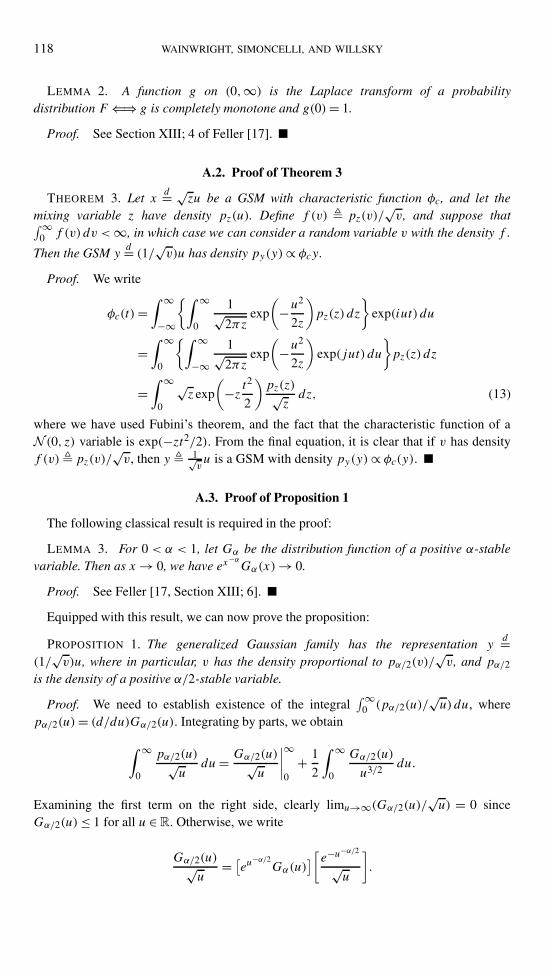
118 WAINWRIGHT, SIMONCELLI, AND WILLSKY
LEMMA 2. A function g on (0,∞) is the Laplace transform of a probabilitydistribution F ⇐⇒ g is completely monotone and g(0)= 1.
Proof. See Section XIII; 4 of Feller [17].
A.2. Proof of Theorem 3
THEOREM 3. Let xd= √
zu be a GSM with characteristic function φc, and let themixing variable z have density pz(u). Define f (v) � pz(v)/
√v, and suppose that∫ ∞
0 f (v) dv <∞, in which case we can consider a random variable v with the density f .
Then the GSM yd= (1/√v)u has density py(y)∝ φcy .
Proof. We write
φc(t)=∫ ∞
−∞
{∫ ∞
0
1√2πz
exp
(−u
2
2z
)pz(z) dz
}exp(iut) du
=∫ ∞
0
{∫ ∞
−∞1√2πz
exp
(−u
2
2z
)exp(jut) du
}pz(z) dz
=∫ ∞
0
√z exp
(−z t
2
2
)pz(z)√zdz, (13)
where we have used Fubini’s theorem, and the fact that the characteristic function of aN (0, z) variable is exp(−zt2/2). From the final equation, it is clear that if v has densityf (v)� pz(v)/
√v, then y � 1√
vu is a GSM with density py(y)∝ φc(y).
A.3. Proof of Proposition 1
The following classical result is required in the proof:
LEMMA 3. For 0 < α < 1, let Gα be the distribution function of a positive α-stablevariable. Then as x→ 0, we have ex
−αGα(x)→ 0.
Proof. See Feller [17, Section XIII; 6].
Equipped with this result, we can now prove the proposition:
PROPOSITION 1. The generalized Gaussian family has the representation yd=
(1/√v)u, where in particular, v has the density proportional to pα/2(v)/
√v, and pα/2
is the density of a positive α/2-stable variable.
Proof. We need to establish existence of the integral∫ ∞
0 (pα/2(u)/√u) du, where
pα/2(u)= (d/du)Gα/2(u). Integrating by parts, we obtain
∫ ∞
0
pα/2(u)√u
du= Gα/2(u)√u
∣∣∣∣∞
0+ 1
2
∫ ∞
0
Gα/2(u)
u3/2du.
Examining the first term on the right side, clearly limu→∞(Gα/2(u)/√u) = 0 since
Gα/2(u)≤ 1 for all u ∈ R. Otherwise, we write
Gα/2(u)√u
= [eu
−α/2Gα(u)
][e−u−α/2√u
].
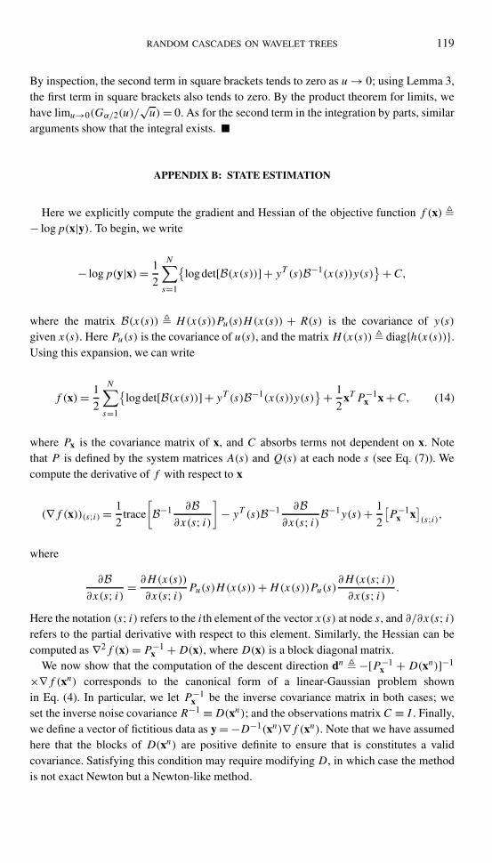
RANDOM CASCADES ON WAVELET TREES 119
By inspection, the second term in square brackets tends to zero as u→ 0; using Lemma 3,the first term in square brackets also tends to zero. By the product theorem for limits, wehave limu→0(Gα/2(u)/
√u)= 0. As for the second term in the integration by parts, similar
arguments show that the integral exists.
APPENDIX B: STATE ESTIMATION
Here we explicitly compute the gradient and Hessian of the objective function f (x)�− logp(x|y). To begin, we write
− logp(y|x)= 1
2
N∑s=1
{log det[B(x(s))] + yT (s)B−1(x(s))y(s)
} +C,
where the matrix B(x(s)) � H(x(s))Pu(s)H(x(s)) + R(s) is the covariance of y(s)given x(s). Here Pu(s) is the covariance of u(s), and the matrix H(x(s))� diag{h(x(s))}.Using this expansion, we can write
f (x)= 1
2
N∑s=1
{log det[B(x(s))] + yT (s)B−1(x(s))y(s)
} + 1
2xT P−1
x x +C, (14)
where Px is the covariance matrix of x, and C absorbs terms not dependent on x. Notethat P is defined by the system matrices A(s) and Q(s) at each node s (see Eq. (7)). Wecompute the derivative of f with respect to x
(∇f (x))(s;i) = 1
2trace
[B−1 ∂B
∂x(s; i)]
− yT (s)B−1 ∂B∂x(s; i)B
−1y(s)+ 1
2
[P−1
x x](s;i),
where
∂B∂x(s; i) = ∂H(x(s))
∂x(s; i) Pu(s)H(x(s))+H(x(s))Pu(s)∂H(x(s; i))∂x(s; i) .
Here the notation (s; i) refers to the ith element of the vector x(s) at node s, and ∂/∂x(s; i)refers to the partial derivative with respect to this element. Similarly, the Hessian can becomputed as ∇2f (x)= P−1
x +D(x), where D(x) is a block diagonal matrix.We now show that the computation of the descent direction dn � −[P−1
x + D(xn)]−1
×∇f (xn) corresponds to the canonical form of a linear-Gaussian problem shownin Eq. (4). In particular, we let P−1
x be the inverse covariance matrix in both cases; weset the inverse noise covarianceR−1 ≡D(xn); and the observations matrix C ≡ I . Finally,we define a vector of fictitious data as y = −D−1(xn)∇f (xn). Note that we have assumedhere that the blocks of D(xn) are positive definite to ensure that is constitutes a validcovariance. Satisfying this condition may require modifying D, in which case the methodis not exact Newton but a Newton-like method.
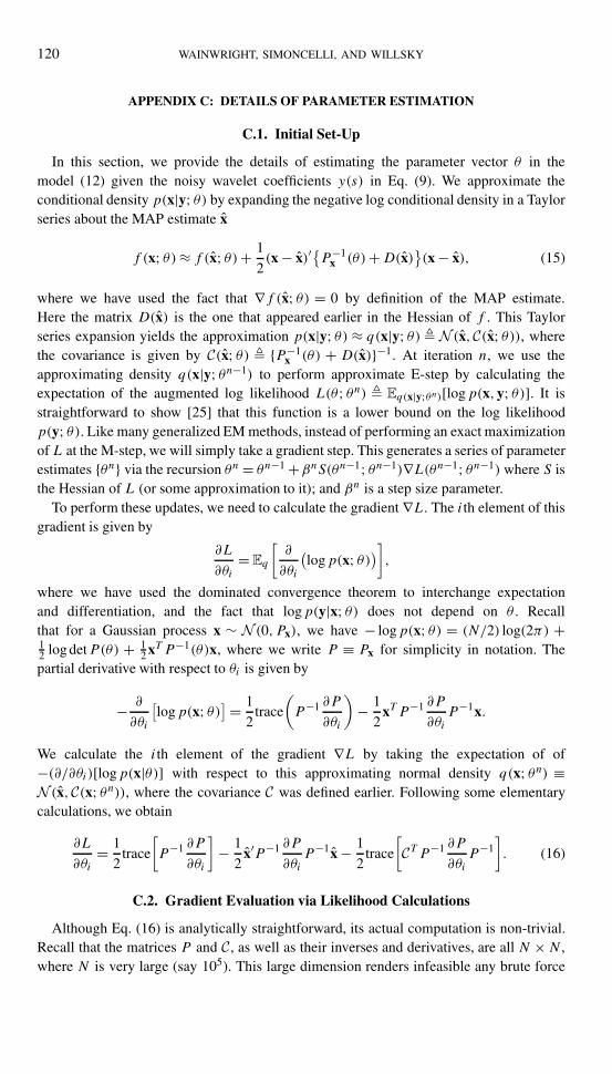
120 WAINWRIGHT, SIMONCELLI, AND WILLSKY
APPENDIX C: DETAILS OF PARAMETER ESTIMATION
C.1. Initial Set-Up
In this section, we provide the details of estimating the parameter vector θ in themodel (12) given the noisy wavelet coefficients y(s) in Eq. (9). We approximate theconditional density p(x|y; θ) by expanding the negative log conditional density in a Taylorseries about the MAP estimate x
f (x; θ)≈ f (x; θ)+ 1
2(x − x)′
{P−1
x (θ)+D(x)}(x − x), (15)
where we have used the fact that ∇f (x; θ) = 0 by definition of the MAP estimate.Here the matrix D(x) is the one that appeared earlier in the Hessian of f . This Taylorseries expansion yields the approximation p(x|y; θ) ≈ q(x|y; θ)� N (x,C(x; θ)), wherethe covariance is given by C(x; θ) � {P−1
x (θ) + D(x)}−1. At iteration n, we use theapproximating density q(x|y; θn−1) to perform approximate E-step by calculating theexpectation of the augmented log likelihood L(θ; θn) � Eq(x|y;θn)[logp(x,y; θ)]. It isstraightforward to show [25] that this function is a lower bound on the log likelihoodp(y; θ). Like many generalized EM methods, instead of performing an exact maximizationof L at the M-step, we will simply take a gradient step. This generates a series of parameterestimates {θn} via the recursion θn = θn−1 +βnS(θn−1; θn−1)∇L(θn−1; θn−1) where S isthe Hessian of L (or some approximation to it); and βn is a step size parameter.
To perform these updates, we need to calculate the gradient ∇L. The ith element of thisgradient is given by
∂L
∂θi= Eq
[∂
∂θi
(logp(x; θ))
],
where we have used the dominated convergence theorem to interchange expectationand differentiation, and the fact that logp(y|x; θ) does not depend on θ . Recallthat for a Gaussian process x ∼ N (0,Px), we have − logp(x; θ) = (N/2) log(2π) +12 log detP(θ) + 1
2 xT P−1(θ)x, where we write P ≡ Px for simplicity in notation. Thepartial derivative with respect to θi is given by
− ∂
∂θi
[logp(x; θ)] = 1
2trace
(P−1 ∂P
∂θi
)− 1
2xT P−1 ∂P
∂θiP−1x.
We calculate the ith element of the gradient ∇L by taking the expectation of of−(∂/∂θi)[logp(x|θ)] with respect to this approximating normal density q(x; θn) ≡N (x,C(x; θn)), where the covariance C was defined earlier. Following some elementarycalculations, we obtain
∂L
∂θi= 1
2trace
[P−1 ∂P
∂θi
]− 1
2x′P−1 ∂P
∂θiP−1x − 1
2trace
[CT P−1 ∂P
∂θiP−1
]. (16)
C.2. Gradient Evaluation via Likelihood Calculations
Although Eq. (16) is analytically straightforward, its actual computation is non-trivial.Recall that the matrices P and C , as well as their inverses and derivatives, are all N ×N ,where N is very large (say 105). This large dimension renders infeasible any brute force
RANDOM CASCADES ON WAVELET TREES 121
approach. However, the tree structure can be exploited to develop a very fast algorithmfor likelihood calculation of MAR models (see [59]), consisting of a single upward sweepfrom leaves to root.
This algorithm for computing MAR likelihoods turns out to be useful here. By applyingthe matrix inversion lemma to Eq. (16) and simplifying, we have
∂L
∂θi= −1
2x′P−1 ∂P
∂θiP−1x + 1
2trace
[(P +D−1)−1 ∂P
∂θi
].
For any covariance matrix �, let J (u;�)� 12 trace log(�)+ 1
2 uT �−1u be the correspond-ing Gaussian likelihood. With this definition, it can be shown be shown that
∂L
∂θi(x)= ∂J
∂θi(P ; x)− ∂J
∂θi(P ; 0)+ ∂J
∂θi(P +D−1; 0).
Thus, the gradient computation can be performed by taking derivatives of standardGaussian likelihoods on the tree. Similarly, this structure permits efficient computationof elements of the Hessian.
REFERENCES
1. D. F. Andrews and C. L. Mallows, Scale mixtures of normal distributions, J. Roy. Statist. Soc. 36 (1974),99–102.
2. D. P. Bertsekas, “Nonlinear Programming,” Athena Sci., Belmont, MA, 1995.
3. R. W. Buccigrossi and E. P. Simoncelli, Image compression via joint statistical characterization in the waveletdomain, IEEE Trans. Image Proc. 8, No. 12 (1999), 1688–1701.
4. A. Chambolle, R. A. DeVore, N. Lee, and B. J. Lucier, Nonlinear wavelet image processing: Variationalproblems, compression, and noise removal through wavelet shrinkage, IEEE Trans. Image Proc. 7 (1998),319–335.
5. S. G. Chang, B. Yu, and M. Vetterli, Spatially adaptive wavelet thresholding with context modeling for imagedenoising, in “Proc. IEEE ICIP,” pp. 535–539, 1998.
6. W. H. Chen and C. H. Smith, Adaptive coding of monochrome and color images, IEEE Trans. Comm. COM-25 (1977), 1285–1292.
7. H. Cheng and C. A. Bouman, Trainable context model for multiscale segmentation, in “Proc. IEEE ICIP,”Vol. 1, pp. 610–614, 1998.
8. K. Chou, A. Willsky, and R. Nikoukhah, Multiscale systems, Kalman filters, and Riccati equations, IEEE
Trans. AC 39, No. 3 (1994), 479–492.
9. C. Chrysafis and A. Ortega, Efficient context based entropy coding for lossy wavelet image compression,in “Proc. Data Compression Conference,” pp. 241–250, 1997.
10. M. S. Crouse, R. D. Nowak, and R. G. Baraniuk, Wavelet-based statistical signal processing using hiddenMarkov models, IEEE Trans. Signal Process. 46 (1998), 886–902.
11. M. Daniel and A. Willsky, Modeling and estimation of fractional Brownian motion using multiresolutionstochastic processes, in “Fractals in Engineering” (J. L. Vehel, E. Lutton, and C. Tricot, Eds.), pp. 124–137,Springer-Verlag, Berlin/New York, 1997.
12. M. Daniel and A. Willsky, The modeling and estimation of statistically self-similar processes in amultiresolution framework, IEEE Trans. Inform. Theory 45, No. 3 (1999), 955–970.
13. J. W. Demmel, “Applied Numerical Linear Algebra,” SIAM, Philadelphia, 1997.
14. A. P. Dempster, N. M. Laird, and D. B. Rubin, Maximum likelihood from incomplete data via the EMalgorithm (with discussion), J. Roy. Statist. Soc. B 39 (1977), 1–38.
122 WAINWRIGHT, SIMONCELLI, AND WILLSKY
15. D. L. Donoho and I. M. Johnstone, Adapting to unknown smoothness via wavelet shrinkage, J. Amer. Statist.Assoc. 90, No. 432 (1995), 1200–1224.
16. B. Efron and C. N. Morris, Limiting the risk of Bayes and empirical Bayes estimators—Part II: The empiricalBayes case, J. Amer. Statist. Assoc. 67 (1972), 130–139.
17. W. Feller, “An Introduction to Probability Theory and Its Applications: Volume II,” Wiley, New York, 1966.
18. P. Fieguth and A. Willsky, Fractal estimation using models on multiscale trees, IEEE Trans. Signal Process.
44, No. 5 (1996), 1297–1300.
19. D. J. Field, Relations between the statistics of natural images and the response properties of cortical cells,J. Opt. Soc. Amer. A 4, No. 12 (1987), 2379–2394.
20. C. W. Harrison, Experiments with linear prediction in television, Bell Syst. Tech. J. 31 (1952), 764–783.
21. J. Huang and D. Mumford, Statistics of natural images and models, CVPR 1 (1999), 547.
22. W. Irving, P. Fieguth, and A. Willsky, An overlapping tree approach to multiscale stochastic modeling andestimation, IEEE Trans. Image Process. 6, No. 11 (1997).
23. W. James and C. Stein, Estimation with quadratic loss, in “Proceedings of the Fourth Berkeley Symposiumon Mathematical Statistics and Probability,” Vol. 1, pp. 361–379, 1961.
24. A. H. Jazwinski, “Stochastic Processes and Filtering Theory,” Academic Press, New York, 1970.
25. M. Jordan, Z. Ghahramani, T. Jaakkola, and L. Saul, Learning in graphical models, in “An Introduction toVariational Methods for Graphical Models,” pp. 105–161, MIT Press, Cambridge, MA, 1999.
26. G. G. Judge and M. E. Bock “The Statistical Implications of Pre-Test and Stein-Rule Estimators inEconometrics,” North-Holland, Amsterdam, 1978.
27. A. Lee and D. Mumford, An occlusion model generating scale-invariant images, preprint available at:http://www.dam.brown.edu/people/mumf.
28. J. S. Lee, Digital image enhancement and noise filtering by use of local statistics, IEEE Pattern Anal. Mach.Intell. PAMI-2 (1980), 165–168.
29. J. Liu and P. Moulin, Image denoising based on scale-space mixture modeling of wavelet coefficients,in “Proc. IEEE ICIP,” Vol. 1, pp. 386–390, 1999.
30. S. LoPresto, K. Ramchandran, and M. Orchard, Image coding based on mixture modeling of waveletcoefficents and a fast estimation-quantization framework, in “Proc. Data Compression Conf.,” 1997.
31. M. Luettgen, “Image Processing with Multiscale Stochastic Models,” Ph.D. thesis, Massachusetts Institute ofTechnology, 1993.
32. M. Luettgen, W. Karl, and A. Willsky, Efficient multiscale regularization with application to optical flow,IEEE Trans. Image Process. 3, No. 1 (1994), 41–64.
33. M. Luettgen, W. Karl, A. Willsky, and R. Tenney, Multiscale representations of Markov random fields, IEEE
Trans. Signal Process. 41, No. 12 (1993), 3377–3396.
34. S. G. Mallat, A theory for multiresolution signal decomposition: The wavelet representation, IEEE PatternAnal. Mach. Intell. 11 (1989), 674–693.
35. M. Mihçak, I. Kozintsev, and K. Ramchandran, Spatially adaptive statistical modeling of wavelet imagecoefficients, and its application to denoising, in “Proc. IEEE ICASSP,” pp. 3253–3256, 1999.
36. M. Mihçak, I. Kozintsev, K. Ramchandran, and P. Moulin, Low-complexity image denoising based onstatistical modeling of wavelet coefficients, IEEE Signal Process. Lett. 6 (1999), 300–303.
37. P. Moulin and J. Liu, Analysis of multiresolution image denoising schemes using a generalized Gaussian andcomplexity priors, IEEE Trans. Inform. Theory 45 (1999), 909–919.
38. D. Mumford and B. Gidas, Stochastic models for generic images, preprint available at http://www.dam.brown.edu/people/mumford.
39. B. M. Oliver, Efficient coding, Bell System Tech. J. 31 (1952), 724–750.
40. A. Pentland, Fractal based description of natural scenes, IEEE Trans. PAMI 6, No. 6 (1984), 661–674.
41. J. Portilla and E. P. Simoncelli, A parametric texture model based on joint statistics of complex waveletcoefficients, Internat. J. Comput. Vision 40, No. 1 (2000), 49–70.
42. H. Rauch, F. Tung, and C. Striebel, Maximum likelihood estimates of linear dynamic systems, AIAA J. 3,No. 8 (1965), 1445–1450.
RANDOM CASCADES ON WAVELET TREES 123
43. J. Romberg, H. Choi, and R. Baraniuk, Bayesian wavelet domain image modeling using hidden Markov trees,in “Proc. IEEE ICIP, Kobe, Japan, October 1999.”
44. D. L. Ruderman, Origins of scaling in natural images, Vision Res. 37 (1997), 3385–3395.
45. D. L. Ruderman and W. Bialek, Statistics of natural images: Scaling in the woods, Phys. Rev. Lett. 73, No. 6(1994), 814–817.
46. G. Samorodnitsky and M. Taqqu, “Stable Non-Gaussian Random Processes: Stochastic Models with InfiniteVariance,” Chapman Hall, New York, 1994.
47. J. M. Shapiro, Embedded image coding using zerotrees of wavelet coefficients, IEEE Trans. Signal Process.41 (1993), 3445–3462.
48. E. P. Simoncelli, Statistical models for images: Compression, restoration and synthesis, in “31st AsilomarConf., IEEE Sig. Proc. Soc., November 1997,” pp. 673–678.
49. E. P. Simoncelli, Bayesian denoising of visual images in the wavelet domain, in “Bayesian Inference inWavelet Based Models” (P. Müller and B. Vidakovic, Eds.), Lecture Notes in Statistics, Vol. 141, Chap. 18,pp. 291–308, Springer-Verlag, New York, 1999.
50. E. P. Simoncelli and E. H. Adelson, Noise removal via Bayesian wavelet coring, in “Third Int. Conf. on ImageProc.,” Vol. I, pp. 379–382, 1996.
51. E. P. Simoncelli and W. T. Freeman, The steerable pyramid: A flexible architecture for multi-scale derivativecomputation, in “Int. Conf. Image Proc.,” Vol. III, pp. 444–447, IEEE Sig. Proc. Soc., Washington, DC, 1995.
52. V. Strela, J. Portilla, and E. P. Simoncelli, Image denoising using a local Gaussian scale mixture model in thewavelet domain, in “Proceedings of SPIE, San Diego, CA, July 2000.”
53. A. H. Tewfik and M. Kim, Correlation structure of the discrete wavelet coefficients of fractional Brownianmotion, IEEE Trans. Inform. Theory 38 (1992), 904–909.
54. A. Turiel, G. Mato, N. Parga, and J. P. Nadal, The self-similarity properties of natural images resemble thoseof turbulent flows, Phys. Rev. Lett. 80 (1998), 1098–1101.
55. M. J. Wainwright and E. P. Simoncelli, Scale mixtures of Gaussians and the statistics of natural images,in “Neural Information Processing Systems 12,” Vol. 12, pp. 855–861, 1999. [Paper available at http://ssg.mit.edu/group/mjwain/mjwain.shtml.]
56. M. J. Wainwright, E. P. Simoncelli, and A. S. Willsky, Random cascades of Gaussian scale mixtures and theiruse in modeling natural images with application to denoising, in “IEEE Int. Conf. Image Proc., Vancouver,Canada, September 2000.”
57. M. J. Wainwright, E. P. Simoncelli, and A. S. Willsky, Random cascades of Gaussian scale mixtures onwavelet trees with application to natural images, in “Proceedings of SPIE, San Diego, CA, July 2000.” [Paperavailable at http://ssg.mit.edu/group/mjwain/mjwain.shtml.]
58. M. J. Wainwright, E. B. Sudderth, and A. S. Willsky, Tree-based modeling and estimation of Gaussianprocesses on graphs with cycles, in “Neural Information Processing Systems 13,” 2000. [Paper availableat http://ssg.mit.edu/group/mjwain/mjwain.shtml.]
59. R. B. Washburn, W. I. Irving, J. K. Johnson, D. S. Artgis, J. W. Wissinger, R. P. Tenney, and A. S. Willsky,Multiresolution image compression and image fusion algorithms, Technical report, Alphatech Company,February 1996.
60. G. Wornell, Wavelet-based representations for the 1/f family of fractal processes, Proc. IEEE (1993).
61. C. Zetzsche, B. Wegmann, and E. Barth, Nonlinear aspects of primary vision: Entropy reduction beyonddecorrelation, in “Int. Symp. Soc. for Info. Display,” Vol. 24, pp. 933–936, 1993.
62. H. Brehm and W. Stammler, Description and generation of spherically invariant speech-model signals, SignalProcess. 12 (1987), 119–141.
63. T. Bollerslev, K. Engle, and D. Nelson, ARCH models, in “Handbook of Econometrics, V.” (B. Engle andD. McFadden, Eds.), 1994.