Embed Size (px)
Citation preview
Assessment of Random-noise Contamination inDigital Images via Testing on Wavelet Coefficients
Sharad Silwal1 and Haiyan Wang2∗ and Diego Maldonado3
1Department of Mathematics, Northland College, 1411 Ellis Avenue Ashland, WI 548062Department of Statistics, Kansas State University, Manhattan, KS 66506
3Department of Mathematics, Kansas State University, Manhattan, KS 66506
Abstract:Full-reference image quality assessment methods seek to measure visual similarity between
two images (in practice, one original and the other its altered version). It has been establishedthat traditional methods, such as Mean Square Error and Peak Signal-to-Noise Ratio poorlymimic the human visual system and much of the recent research in image quality assessmenthas been directed toward developing image similarity measures that are more consistent withassessments from human observers. Some extensively tested popular methods in this regardare Visual Image Fidelity (VIF), Structure Similarity Index (SSIM) and its variants Multi-scaleStructure Similarity Index (MS-SSIM) and Information Content Weighted Multi-scale Struc-ture Similarity Index (IW-SSIM). However, experiments show that these methods may pro-duce drastically different similarity indices for different images contaminated with the samesource of random noise. In this article, we propose a new full-reference image quality assess-ment method, namely, Wavelet-based Non-parametric Structure Similarity Index (WNPSSIM),specifically designed to detect visual similarity between images contaminated with all sorts ofrandom noises. WNPSSIM is based on a rank test of the hypothesis of identical images con-ducted on the wavelet domain. Our experimental comparisons demonstrate that WNPSSIMprovides similar ranking as MS-SSIM, IW-SSIM and VIF for images contaminated with differ-ent random noises in general though the methodology is very different. In addition, WNPSSIMcorrects the aforementioned shortcoming of assigning sharply different similarity indices fordifferent images contaminated with the same source of random noise.
AMS 2000 subject classifications: Primary 68U10, 97K80, 62H35; secondary 62G10.Keywords and phrases: Image structure similarity, nonparametric hypothesis testing, Full-Reference, human visual system (HVS), Discrete Wavelet Transform (DWT).
1. Introduction
Digital imaging has found massive applications in many branches of science: astronomy, mete-orology, seismology, industrial inspection, aerial reconnaissance, autonomous navigation, to namebut a few. As such, a reliable image quality index is highly desirable and vigorously pursued by theresearch community. In the literature, we find three generic approaches to an image quality assess-ment method; namely, full-reference, reduced-reference and no-reference. A full-reference imagequality assessment method measures the visual similarity of a test image with respect to a supplied
∗Corresponding author e-mail: [email protected], Phone: 785-532-0519.
1
Silwal, Wang, and Maldonado, 2011/WNPSSIM 2
reference image. It is applicable when a true image or a standard reference image is known, suchas in image compression and image coding (Richter and Larabi [2008]).
Many full-reference image quality assessment methods can be found in the literature. Multi-scale Structure Similarity Index (MS-SSIM) (Wang et al. [2003]), Visual Image Fidelity (VIF)(Sheikh and Bovik [2006]), and Information Content Weighted Multi-scale Structure SimilarityIndex (IW-SSIM) (Wang and Li [2011]) are popular image quality assessment methods which areextensively tested and widely recognized to be consistent with the HVS. Others are Wang et al.[2004], Wang and Simoncelli [2005a], Sheikh et al. [2005a], Ninassi et al. [2006], Chandler andHemami [2007], Gao et al. [2009] and Wang et al. [2011]. We found that the extent to which thesemethods are capable of seeing through random noises in the same way the human visual system(HVS) does is limited. As a result, they may assign drastically different similarity index values forimages contaminated with the same source of random noise. In practice, random noise is inevitablyabundant in digital images. They occur at every stage of image acquisition and processing and theyare quite difficult to remove completely. Thus, some level of random noise is always assumed inalmost all forms of digital images. Moreover, if the contamination level of the random noise islow, the HVS easily sees through it and recognizes the underlying true image. This property of theHVS is the main focus of interest in this paper as it concentrates on developing an image similarityassessment method which possesses the ability to see through moderate amounts of random noisein images in the same manner as the HVS does and is robust for all types of random noises.
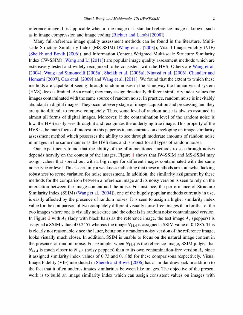
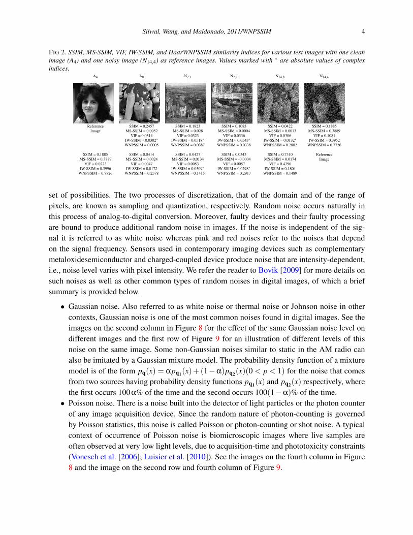
Our experiments found that the ability of the aforementioned methods to see through noisesdepends heavily on the content of the images. Figure 1 shows that IW-SSIM and MS-SSIM mayassign values that spread out with a big range for different images contaminated with the samenoise type or level. This is certainly a weakness indicating that these methods are somewhat lackingrobustness to scene variation for noise assessment. In addition, the similarity assignment by thesemethods for the comparison between a reference image and its noisy version is seen to rely on theinteraction between the image content and the noise. For instance, the performance of StructureSimilarity Index (SSIM) (Wang et al. [2004]), one of the hugely popular methods currently in use,is easily affected by the presence of random noises. It is seen to assign a higher similarity indexvalue for the comparison of two completely different visually noise-free images than for that of thetwo images where one is visually noise-free and the other is its random noise contaminated version.In Figure 2 with A4 (lady with black hair) as the reference image, the test image A8 (peppers) isassigned a SSIM value of 0.2457 whereas the image N14,4 is assigned a SSIM value of 0.1885. Thisis clearly not reasonable since the latter, being only a random noisy version of the reference image,looks visually much closer. In addition, SSIM is unable to focus on the natural image content inthe presence of random noise. For example, when N14,4 is the reference image, SSIM judges thatN14,4 is much closer to N14,8 (noisy peppers) than to its own contamination-free version A4 sinceit assigned similarity index values of 0.73 and 0.1885 for these comparisons respectively. VisualImage Fidelity (VIF) introduced in Sheikh and Bovik [2006] has a similar drawback in addition tothe fact that it often underestimates similarities between like images. The objective of the presentwork is to build an image similarity index which can assign consistent values on images with
Silwal, Wang, and Maldonado, 2011/WNPSSIM 3
random noise contamination visible to the eye without being adversely affected by the contents inimages.
We will first briefly list typical random noises that are common in digital images, since identify-ing the nature of these noise sources is critical to the development of quality assessment methodsunder realistic assumptions. The fact that different noises follow different distributions motivatesus to propose an image quality assessment method based on non-parametric statistics. We will thenreview some image quality assessment methods with brief discussion of their relevance to the con-text of this paper and the reason they may yield quality indices inconsistent with the HVS. Thenwe will describe our new wavelet-based image similarity assessment method which is developedthrough a non-parametric test on hypotheses related to the wavelet coefficients of the reference andtest images. We illustrate with experiments that the proposed image similarity index WNPSSIMprovides a more realistic similarity assessment of images contaminated with random noise.
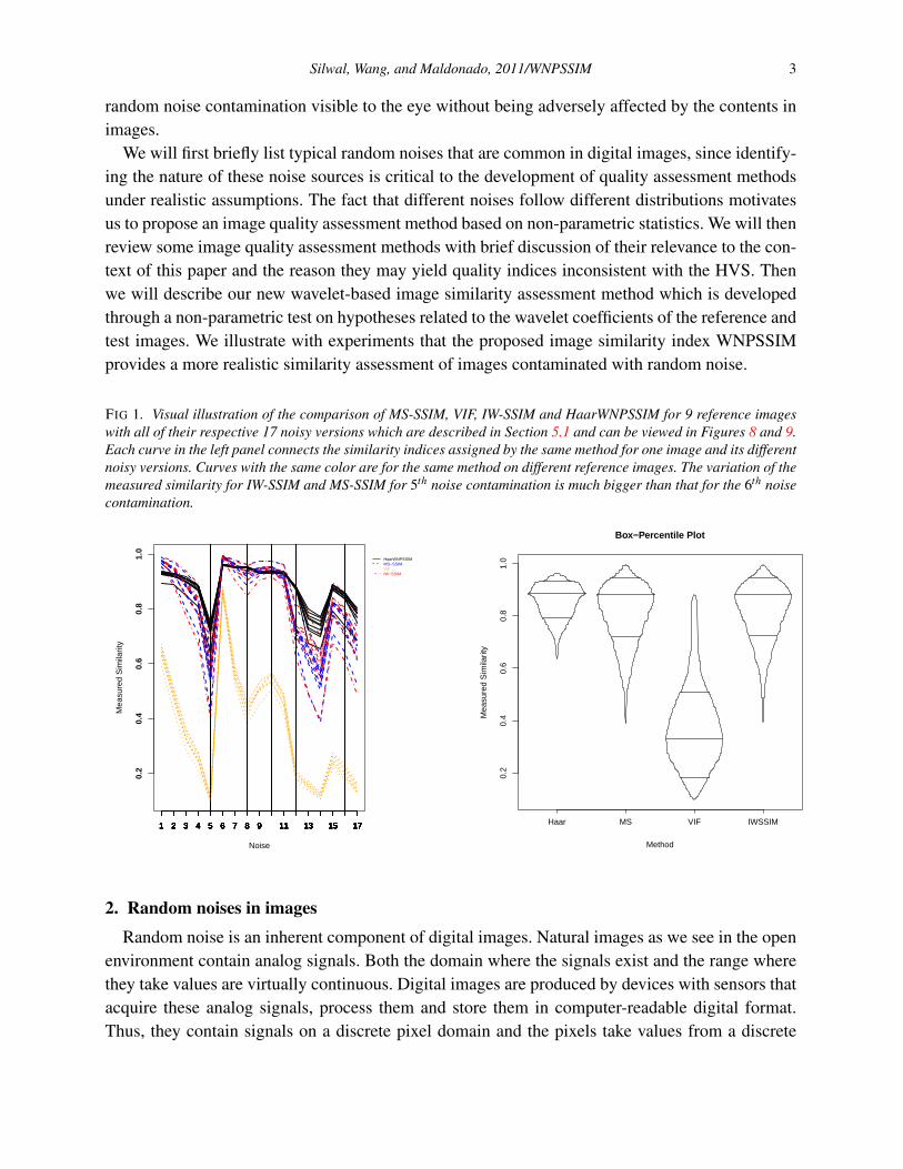
FIG 1. Visual illustration of the comparison of MS-SSIM, VIF, IW-SSIM and HaarWNPSSIM for 9 reference imageswith all of their respective 17 noisy versions which are described in Section 5.1 and can be viewed in Figures 8 and 9.Each curve in the left panel connects the similarity indices assigned by the same method for one image and its differentnoisy versions. Curves with the same color are for the same method on different reference images. The variation of themeasured similarity for IW-SSIM and MS-SSIM for 5th noise contamination is much bigger than that for the 6th noisecontamination.
0.2
0.4
0.6
0.8
1.0
Noise
Mea
sure
d S
imila
rity
1 2 3 4 5 6 7 8 9 11 13 15 171 2 3 4 5 6 7 8 9 11 13 15 171 2 3 4 5 6 7 8 9 11 13 15 171 2 3 4 5 6 7 8 9 11 13 15 171 2 3 4 5 6 7 8 9 11 13 15 171 2 3 4 5 6 7 8 9 11 13 15 171 2 3 4 5 6 7 8 9 11 13 15 171 2 3 4 5 6 7 8 9 11 13 15 171 2 3 4 5 6 7 8 9 11 13 15 17
HaarWNPSSIMMS−SSIMVIFIW−SSIM
0.2
0.4
0.6
0.8
1.0
Box−Percentile Plot
Mea
sure
d S
imila
rity
Method
Haar MS VIF IWSSIM
2. Random noises in images
Random noise is an inherent component of digital images. Natural images as we see in the openenvironment contain analog signals. Both the domain where the signals exist and the range wherethey take values are virtually continuous. Digital images are produced by devices with sensors thatacquire these analog signals, process them and store them in computer-readable digital format.Thus, they contain signals on a discrete pixel domain and the pixels take values from a discrete
Silwal, Wang, and Maldonado, 2011/WNPSSIM 4
FIG 2. SSIM, MS-SSIM, VIF, IW-SSIM, and HaarWNPSSIM similarity indices for various test images with one cleanimage (A4) and one noisy image (N14,4) as reference images. Values marked with ∗ are absolute values of complexindices.
A4 A8 N2,1 N7,2 N14,8 N14,4
Reference SSIM = 0.2457 SSIM = 0.1823 SSIM = 0.1083 SSIM = 0.0422 SSIM = 0.1885Image MS-SSIM = 0.0052 MS-SSIM = 0.028 MS-SSIM = 0.0004 MS-SSIM = 0.0013 MS-SSIM = 0.3889
VIF = 0.0314 VIF = 0.0323 VIF = 0.0336 VIF = 0.0306 VIF = 0.1081IW-SSIM = 0.0302∗ IW-SSIM = 0.0518∗ IW-SSIM = 0.0543∗ IW-SSIM = 0.0132∗ IW-SSIM = 0.3952WNPSSIM = 0.0005 WNPSSIM = 0.0387 WNPSSIM = 0.0338 WNPSSIM = 0.2882 WNPSSIM = 0.7726
SSIM = 0.1885 SSIM = 0.0414 SSIM = 0.0427 SSIM = 0.0343 SSIM = 0.7310 ReferenceMS-SSIM = 0.3889 MS-SSIM = 0.0024 MS-SSIM = 0.0134 MS-SSIM = -0.0004 MS-SSIM = 0.0174 Image
VIF = 0.0223 VIF = 0.0047 VIF = 0.0053 VIF = 0.0057 VIF = 0.4396IW-SSIM = 0.3996 IW-SSIM = 0.0172 IW-SSIM = 0.0309∗ IW-SSIM = 0.0298∗ IW-SSIM = 0.1804
WNPSSIM = 0.7726 WNPSSIM = 0.2578 WNPSSIM = 0.1415 WNPSSIM = 0.2917 WNPSSIM = 0.1489
set of possibilities. The two processes of discretization, that of the domain and of the range ofpixels, are known as sampling and quantization, respectively. Random noise occurs naturally inthis process of analog-to-digital conversion. Moreover, faulty devices and their faulty processingare bound to produce additional random noise in images. If the noise is independent of the sig-nal it is referred to as white noise whereas pink and red noises refer to the noises that dependon the signal frequency. Sensors used in contemporary imaging devices such as complementarymetaloxidesemiconductor and charged-coupled device produce noise that are intensity-dependent,i.e., noise level varies with pixel intensity. We refer the reader to Bovik [2009] for more details onsuch noises as well as other common types of random noises in digital images, of which a briefsummary is provided below.
• Gaussian noise. Also referred to as white noise or thermal noise or Johnson noise in othercontexts, Gaussian noise is one of the most common noises found in digital images. See theimages on the second column in Figure 8 for the effect of the same Gaussian noise level ondifferent images and the first row of Figure 9 for an illustration of different levels of thisnoise on the same image. Some non-Gaussian noises similar to static in the AM radio canalso be imitated by a Gaussian mixture model. The probability density function of a mixturemodel is of the form pq(x) = αpq1(x)+ (1−α)pq2(x)(0 < p < 1) for the noise that comesfrom two sources having probability density functions pq1(x) and pq2(x) respectively, wherethe first occurs 100α% of the time and the second occurs 100(1−α)% of the time.• Poisson noise. There is a noise built into the detector of light particles or the photon counter
of any image acquisition device. Since the random nature of photon-counting is governedby Poisson statistics, this noise is called Poisson or photon-counting or shot noise. A typicalcontext of occurrence of Poisson noise is biomicroscopic images where live samples areoften observed at very low light levels, due to acquisition-time and phototoxicity constraints(Vonesch et al. [2006]; Luisier et al. [2010]). See the images on the fourth column in Figure8 and the image on the second row and fourth column of Figure 9.
Silwal, Wang, and Maldonado, 2011/WNPSSIM 5
• Salt and pepper noise. This is an impulse noise which is very common in digital images. Im-ages corrupted with salt and pepper noise are degraded in only a few random pixel locations.This noise is often the result of faulty memory locations and signal transmission throughnoisy digital links. See the images on the third column in Figure 8 and the first three imageson the second row of Figure 9.• Speckle noise. Another noise that is more common in geoscience imaging such as active
radar, synthetic aperture radar and biomedical imaging such as optical coherence tomog-raphy and ultrasound images is called speckle noise. This noise is produced in the imagingsystem where there are coherent light sources such as lasers or radar transmitters. The sourceof this noise is attributed to random interference of the coherent returns issued from the nu-merous scatterers present on a surface, on the scale of a wavelength of the incident radarwave (Gagnon and Jouan [1997]). In other words, due to the microscopic variations of thesurface roughness within one pixel, when the light is reflected off the surface, the receivedsignal is subjected to random variations in phase and amplitude (Bovik [2009]). See the im-ages on the fifth column in Figure 8 and the last two images on the second row and the firstone on the third row of Figure 9.
3. Some common image similarity assessment methods and their possible limitations
Images get degraded in time naturally or get corrupted through various processes they are subjectto since they are captured. An image similarity assessment method is a measure of the degradationor corruption of an image. Full-reference image similarity assessment methods measure the lossof quality in a noisy image relative to a supplied reference image which is treated as the pure orideal version. In this section, we define and discuss some common full-reference image similarityassessment methods. Let X be an original or reference image and Y be its estimate or a test image,both 8-bit images of size m×n.
3.1. Traditional similarity indicesMost conventional image similarity indices are based on the Euclidean distance or the L2-norm
because it is regarded as the natural distance in most spaces. Let X and Y be images of size m×n.The mean squared error (MSE) of Y with respect to X , the error in terms of the Euclidean distance,is defined as
MSE(X ,Y ) =1
mn‖X−Y‖2
2 =1
mn
m
∑i=1
n
∑j=1|X(i, j)−Y (i, j)|2.
The human eye is regarded to be the true benchmark for image similarity assessment methodswhich is known to process an image in a much more complicated sense, viewing image pixelsen bloc to capture visual similarity. As is clear from the above definition, MSE merely takes intoaccount each individual pixel value without any adjusted weighting in measuring the similaritybetween images. As a result, MSE turns out to be a very poor indicator of visual similarity betweenimages. This has been discussed in great detail along with extensive illustrations in Wang andBovik [2009]. A popular traditional measure of image similarity is Signal-to-Noise Ratio (SNR)
Silwal, Wang, and Maldonado, 2011/WNPSSIM 6
defined as
SNR(X ,Y ) = 10log10
(‖X‖2
2
‖X−Y‖22
).
It is measured in decibel (dB) units. A larger value of SNR in general indicates the presence ofless noise in the image. Since SNR is defined through MSE, it shares the drawbacks of MSE as animage similarity measure. Since MSE, Total Variation (TV), and other similar measures such asL1-norm which are purely mathematical in nature treat each pixel identically, we avoid reiterationof them.
3.2. Structure Similarity Index (SSIM)Introduced first in Wang and Bovik [2002] and fully developed in Wang et al. [2004], a correlation-
based image similarity measure called the Structure Similarity Index (SSIM) emerged as a solidmethod giving more realistic image similarity measures than L2-norm-based methods such as MSEand Signal-to-Noise Ratio (SNR). The introduction of SSIM led to many other full-reference im-age similarity measures in the literature seeking to eliminate some of the limitations of SSIM.Notwithstanding its drawbacks, SSIM is found widely cited in the literature owing to its thoroughconstruction which incorporates several factors of visual perception.
SSIM(X ,Y ) is defined to be the average of all local indices SSIM(x,y), x=X(i, j), y=Y (i, j), i=1, ...,m−10, j = 1, ...,n−10, which, in turn, is the product of three factors:
SSIM(x,y) = l(x,y) · c(x,y) · s(x,y) =
(2µxµy +C1
µ2x +µ2
y +C1
)·
(2σxσy +C2
σ2x +σ2
y +C2
)·(
σxy +C3
σxσy +C3
),
where l(x,y), c(x,y) and s(x,y) are the local luminance comparison, local contrast comparisonand local structure comparison or correlation between the images X and Y respectively. For localstatistics on each pixel , a 11×11 submatrix of X with X(i, j) as the (1,1) entry is chosen and thelocal mean µx is computed for this local window as a weighted mean with the same size Gaussianlow-pass filter with standard deviation 1.5 as the weight matrix. Similarly, the local mean µy, localstandard deviations σx and σy and the local covariance σxy are computed. C1 = 0.01, C2 = 2C3 =
0.03 are small positive constants incorporated to avoid numerical instability. Note the cancelationin the formula for SSIM(x,y) after the choice C2 = 2C3. The SSIM(X ,Y ) described here is thesimplest and default version of the SSIM MATLAB code as made available by Wang et al. [2004].We refer the reader to the original paper for details on a more complete version of SSIM.
The local statistics in SSIM was necessary to account for local variations of image featuresacross a scene and also due to the fact that at typical viewing distances, only a local area in theimage can be perceived with high resolution by the human observer at one time instance. Thelocal smoothing with a low-pass filter was reported to eliminate undesirable “blocking” artifactsand exhibit a locally isotropic property in the SSIM index map (Wang et al. [2004]). Such localsmoothing makes SSIM quite insensitive to boundary or edge loss. This, however, becomes un-favorable when the loss is too much to preserve the visual quality. The third factor in the SSIMformula is Pearson’s correlation which is too naive a measure for structure similarity comparison
Silwal, Wang, and Maldonado, 2011/WNPSSIM 7
since it only quantifies the strength of a linear relationship. It is well-known that Pearson’s cor-relation is a valid measure of dependence between two variables only if one variable is a linearfunction of the other, say Y = Xβ+ ε, and the noise ε has a Gaussian distribution. When the noisedistribution is not Gaussian, it is possible that the correlation between X and Y is zero but X and Yare perfectly related (see Wang et al. [2010] for explicit examples). Indeed, we have found in ourexperiments that SSIM yields persistently high scores for blurred distortions and deceptively lowscores for slight random noisy versions in relation to how the human eye perceives the quality loss.
3.3. MS-SSIM, VIF and IW-SSIMAmong all the full-reference image quality assessment methods in the literature, the three multi-
scale decomposition methods MS-SSIM (Wang et al. [2003]), VIF (Sheikh and Bovik [2006]) andIW-SSIM (Wang and Li [2011]) are most relevant to our article. In most practical purposes (notalways, though, see Figure 2), they have similarity indices on a scale of 0 to 1 (perfect similarity)just like the proposed image quality assessment method in this article. We Refer the reader to theoriginal papers for more detail and only provide here a very brief description of these methods.
MS-SSIM was introduced by some of the co-developers of SSIM as an improvement over SSIM.The methodology involves a multi-scale decomposition of involved images through an iterativeprocess of applying a low-pass filtering and downsampling by 2 in each dimension. It is apt tomention that the standard discrete wavelet transform is very similar to this process as it also appliesa low-pass filtering associated with a particular wavelet followed by downsampling by 2. If thelow-pass filter associated with a particular wavelet are of length 2N, a one-dimensional signal oflength n will reduce to an approximated signal of length equal to the integer less than or equal to(n− 1+ 2N)/2. The final MS-SSIM index is constructed by combining the three components ofSSIM, namely, luminance, contrast and structure computed at different scales. As is the case withSSIM, due to a correlation factor as its component, the values of the MS-SSIM index, in principle,might range between -1 and 1.
VIF, proposed by two of the co-developers of SSIM, uses a statistical approach developed bythe authors in Sheikh et al. [2005a] where the so-called natural images are modeled in the waveletdomain as perceived by the HVS. A more detailed discussion of the natural images in the waveletdomain is provided in Section 4.1. First, the source, distortion and HVS models based on theGaussian Scale Mixture (GSM) model (Wainwright et al. [2001]) are developed. Reference imagesare then modeled as outputs of a natural source having passed through the HVS channel. Distortedimages pass through an additional distortion channel before entering the HVS channel. Next, theimage information is computed as the mutual information between the input and the output of theHVS channel. Finally, the VIF index is computed as the ratio of the distorted image informationand the reference image information. VIF is not a symmetric index and can take on values biggerthan 1 for contrast-enhanced test images. However, for most practical purposes, including the oneconsidered in this paper which restricts the attention to only random-noisy test images, VIF doeslie between 0 and 1.
IW-SSIM is another recent image quality assessment algorithm proposed as an improvementover MS-SSIM. Most methods, including MS-SSIM, provide an elaborate method of measuring

Silwal, Wang, and Maldonado, 2011/WNPSSIM 8
local image similarity and a relatively more simplistic method of pooling those local measure-ments into a global image similarity measure. The main feature of IW-SSIM is a more sophisti-cated way of pooling together local measurements. The authors provide an elaborate formula tocompute weights proportional to local information content based on the image information mea-sure in the VIF index described above. The IW-SSIM index employs the weighted pooling of theSSIM components computed at different scales and locations. In the event of some unconventionalcomparison, the IW-SSIM index can also take complex values (see examples in Figure 2).
3.4. Other image similarity assessment methodsDevelopment of full-reference image quality assessment methods in agreement with the HVS
is one of the highly pursued topics of research in the image processing community. A discussionof several old and new full-reference image quality assessment methods can be found in Pono-marenko et al. [2009a] along with a comparison among them. One of the earlier methods basedon the idea of a wavelet analysis was proposed in Lai and Kuo [2000]. Besides those alreadymentioned, some other methods include Complex Wavelet-domain SSIM (CWSSIM) (Wang andSimoncelli [2005b]), Information Fidelity Criterion (IFC) (Sheikh et al. [2005a]), Peak Signal-to-Noise Ratio human visual system (Egiazarian et al. [2006]), Visual Signal-to-Noise Ratio (Chan-dler and Hemami [2007]) and Peak Signal-to-Noise Ratio taking into account Contrast SensitivityFunction, Between-coefficient Contrast Masking of Discrete Cosine Transform basis functions(Ponomarenko et al. [2009a]).
In Wang et al. [2011], the authors of this article have proposed an image similarity assessmentmethod called P-value-based Structure Similarity Index (PSSIM) which is constructed by applyinga rank-based non-parametric test of independence developed in Wang et al. [2010]. It has beenshown in Wang et al. [2011] that PSSIM consistently outperforms SSIM and MSE as an imagesimilarity index in the context of both random and deterministic noises. The emphasis of PSSIMis on structural loss of image features. Hence, it employs a test of independence which is violatedwhen there is a loss of image structure. By contrast, the goal of this article is to develop an imagesimilarity assessment method with the emphasis on the ability to see through random noise atreasonable levels such that the human eye can still identify the image content of the underlyingimage. Hence, in the construction of the WNPSSIM index proposed in this article, we employa completely different test that appropriately detects the structural difference in the presence ofrandom noise in images by assessing whether or not the noise come from an identical source.Although both PSSIM and the proposed WNPSSIM method employ statistical tests, there is asignificant methodological difference between the two methods. PSSIM employs a test in the pixeldomain and WNPSSIM employs a test in the wavelet domain, where the HVS properties are knownto be better captured. Owing to the pixel-domain methodology of PSSIM and the very specificobjective of this paper, PSSIM is deemed irrelevant to the current context. Thus, we do not provideany more discussion of PSSIM in this paper and the reader is referred to the original article Wanget al. [2011] for its detailed description. Instead, we include in this article comparisons of theproposed method with MS-SSIM, VIF, and IW-SSIM (see Section 3.3) which are more relevant toour current context.

Silwal, Wang, and Maldonado, 2011/WNPSSIM 9
4. Our proposed image similarity assessment method
This section describes the details of our proposed image similarity assessment method. Thismethod employs, in the wavelet domain, a non-parametric test developed by Wang et al. [2008].In Section 4.1, we briefly revisit the wavelet paradigm applied to natural images. A description ofour construction of the proposed similarity index is provided in Section 4.2 and Section 4.3.
4.1. The wavelet domain and the natural images in the wavelet domainThe wavelet transform provides a representation of images that enables a rich image analysis due
to various properties that are not available in the raw image data, i.e., the data in the pixel domain.Moreover, the decay and localization properties of wavelets have made the wavelet domain evenbetter than the Fourier domain where the representative profiles are global sinusoidal signals. Werefer the reader to Daubechies [1992] and Mallat [2008] for a detailed treatment of the waveletand multi-resolution approximation theories. An illustration of the wavelet transform of data in thecontext of images is given in Figure 3, where the image on the left is the data in the pixel domainand the image on the right is the visualization of the data in the wavelet domain which consists ofthe four sets of wavelet coefficients called subbands. In Figure 3, the approximation subband (ap),horizontal subband (h), vertical subband (v) and diagonal subband (d) are represented by the fourblocks: the top left, top right, bottom left and bottom right respectively.
FIG 3. Original image and its Haar subbands at level 1
(a) Original image (b) Haar subbands
Mathematically, all M×N matrices with entries lying in a range of values representing grayscaleintensities, most commonly in {0,1, . . . ,255}, are (monochromatic) images. However, the major-ity of such images neither resemble anything in nature nor are encountered in most applications.The images that are mainly of interest to the image analysis community are the so-called nat-ural images, that is, the images that occur in nature and everyday life. The collection of thesenatural images is believed to be a very thin subset of RMN . Indeed, these images typically havespatial structure mostly consisting of smooth areas interspersed with occasional edges (Simoncelliand Adelson [1996]). This structure, which distinguishes an image as a natural image, is better
Silwal, Wang, and Maldonado, 2011/WNPSSIM 10
explained and exploited via some transformation in domains other than the pixel domain. In theFourier domain, the power spectrum S( f ) of natural images typically possess the decay propertyS( f ) =C f−γ where f is the spatial frequency, C is some constant and γ≈ 2 (Millane et al. [2003];Field [1987]; Tolhurst et al. [1992]; Ruderman [1997]; Field and Brady [1997]). Likewise, naturalimages when transformed into the wavelet domain are also seen to enjoy a number of proper-ties. One is the sparsity of the wavelet coefficients, i.e., most wavelet coefficients are near-zeroand can be discarded for approximation purposes (Mallat [2008]). Second, the sizes of the de-tail wavelet coefficients can be modeled by the following generic probability density function:h(u) = Ke−(|u|/α)β
where α and β are the decay and variance parameters respectively and K is anormalizing constant (Mallat [1989]).
As regards the goal of this paper which is to develop an image similarity method close to thehuman visual system (HVS) in performance, the most important property of the wavelet transformof the natural images is its high similarity with the HVS (Field [1999]; Ninassi et al. [2008]; Xionget al. [1997]). The process of the HVS can be tersely explained in two phases: the pre-processingof the light reflected of an object by the neurons before it enters the visual cortex as an input andthe post-processing thereof by the cortical cells eventually leading to object recognition by thehuman brain. During both phases, the different visual information components are processed by aseries of different and independent channels which are sensitive to the visual stimuli with specificspectrum location, frequency and orientation (Gao et al. [2010]). The wavelet decomposition ofan image exhibits striking similarity with the HVS regarding the independent processing of thedifferent components of an image relative to location and orientation. This property of the HVS isreferred to as multi-channel parallel pathways. Hence, the representation of images in the waveletdomain better captures this property of the HVS by sharing basic properties of neural responses inthe primary visual cortex of mammals which are presumably adapted to efficiently represent thevisually relevant features of images (Portilla et al. [2003]). Thus, keeping in view that the discretewavelet transformation establishes a multiresolution representation which attempts to mimic thedecomposition performed by the cortical basis, all with relatively low complexity (Watson [1987];Chandler and Hemami [2005]), we take the wavelet domain as our natural domain for image qualityassessment.
4.2. The non-parametric test in the context of image similarityWang et al. [2008] have developed a non-parametric test which evaluates whether the observa-
tions in a vector or a signal are independently identically distributed, i.e., iid. This is a rank-basedhypothesis test which is essentially an “iid noise detector”. We refer the reader to Wang et al.[2008] and Wang and Akritas [2004] for details. Our work in this current paper is to measure thesimilarity between the two images, say, the reference image X and the test image Y by applying theabove-mentioned test to the relative difference between them, namely, the ratio X−Y
|X |+|Y | . If Y is somerandom-noise contamination of X , this ratio measures how big the noise at each pixel location isrelative to the images. The denominator may be replaced by X if an asymmetric similarity index isdesired. By testing whether the local ratios are ‘iid’, we obtain a similarity assessment method ofhow far Y departs from X locally and whether this departure is negligible.
Silwal, Wang, and Maldonado, 2011/WNPSSIM 11
We have discussed in Section 4.1 that the signal features relevant to the human visual system(HVS) are better captured by their transforms in the wavelet domain than in the raw pixel domain.Hence, instead of applying the test directly on the difference of the reference image X and the testimage Y , we consider their four first-level subbands, namely, approximation subband (ap), verticaldetail subband (v), horizontal detail subband (h) and diagonal detail subband (d) and apply the testto their relative differences, namely,
Xap−Yap
|Xap|+ |Yap|,
Xv−Yv
|Xv|+ |Yv|,
Xh−Yh
|Xh|+ |Yh|and
Xd−Yd
|Xd|+ |Yd|. (4.1)
A wavelet decomposition of the images in our experiment data was done in MATLAB using theDIPUM package (Gonzalez et al. [2009]). A vast number of choices for wavelets is also availablewith the wavelet toolbox in MATLAB. In our experiment, we have used the five wavelets: Haar,Daubechies 4, Symmlet 4, Jpeg 9.7 and Biorthogonal 6.8. All the five versions of WNPSSIM givea better performance in comparison to other methods. Since the similarity measures assigned bythem are very close to one another, we take HaarWNPSSIM as the representative of all five versionsand only refer to this one in most of our discussions. Further remarks on the types of wavelets andtheir performances are provided in Section 6.1.
Next, we adopt the same principle of incorporating local measurements as was done by SSIM.Instead of applying the test only once to each relative difference of subbands in (4.1), we considermultiple local windows in it and apply the test to each local window. For example, in a localwindow of Xap−Y ap
|Xap|+|Yap| , a non-rejection of the test indicated by a large ‘p-value’ provides evidenceto believe that the relative difference between the two subbands Xap and Yap restricted to thatlocal region is close enough to ‘iid’ random noise (subject to type II error), which, in turn, can beinterpreted as the two subbands having a high level of structural similarity between them in thatlocal window, except for some random noise. We then record the percentage of non-rejections ofthe hypothesis tests applied to the local windows within each subband image and we denote themby pap, ph, pv and pd after approximation, horizontal detail, vertical detail and diagonal detailrespectively.
We emphasize that pap, ph, pv and pd are proportions of non-rejections, and not p-values. Theyhave a more direct meaning in the sense that they represent the proportions of local regions ofthe two images that resemble each other structure-wise in corresponding subbands. This idea ofconsidering the proportion of non-rejections was successfully implemented by the same authorsin Wang et al. [2011] where another image similarity index based on a different rank-based non-parametric test in the spatial domain was proposed and shown to imitate the HVS better than othercontemporary similarity indices, most notably, SSIM. This paper, as we have described above,seeks to focus on the seeing-through ability of random noises of the HVS. Also, note that the ob-jective of our test is the non-rejections of the null hypotheses rather than the rejections which isdifferent from the usual objective of a hypothesis test in most cases. Therefore, we do not rec-ommend to use multiple-comparison adjustments aimed at controlling the family-wise error rate.Instead, a cut-off level of α for non-rejection is more stringent than the threshold by Bonferronicorrected level (≈ α divided by the number of tests). This ensures the p-values need to be large
Silwal, Wang, and Maldonado, 2011/WNPSSIM 12
enough to qualify as a non-rejection. We have implemented in our experiment α = 0.01.All the images in our experiment described in Section 5.1 and partially illustrated in Figures
8 and 9 are of size 512× 512. Each subband is one-fourth the original image size, i.e., of size256×256. For these subbands, we consider local windows of size 11×11, much in the same spiritas that of SSIM. The application of the test on local windows provide local similarity measurementswhich are then pooled together to obtain a global similarity measurement. In choosing the size fora shift of a local window so as to cover the whole image, there is a trade-off between the amount oflocal comparisons to take into account and the computational cost. A local window of size 11×11and its horizontal or vertical shift by only 1 pixel differ, at the most, at 11 observations out of atotal of 121 observations. As a result, the p-values produced with the test applied with respect tothese two local windows are almost identical. On the other hand, the intersection of the windowsis also necessary, to some extent, to ensure that the spatial connection within the local regions ofthe two images is carried over to the final similarity measurement between them. Hence, in orderto strike a balance, our rule is to shift the local windows horizontally and then vertically by half ofthe window width, namely, by 5 pixel locations.
With the proportions of non-rejections pap, ph, pv and pd corresponding to the four subbands de-fined in this section, a similarity index between the reference image and the test image is calculatedas a weighted geometric mean of these proportions as below:
WSSIM = p0.95ap · p0.02
h · p0.02v · p0.01
d .
The weighted mean WSSIM is so constructed as to give proper credential to each subband tothe extent it supplies structural information to the HVS. Note that all the proportions as well asweights are positive numbers less than one. Hence, raising the proportions of non-rejections fromeach subband to such weights has the effect of boosting those proportions. The construction ofthe weighted geometric mean WSSIM is based on the idea that a proportion that is to be givenless importance is assigned a smaller weight and is boosted thereof. The weights, as assigned,reflect that WSSIM honors more of the conclusion from the approximation subband and pays lessattention to the detail subbands. We list below a few points to justify our approach:
1. The approximation subband is a subsampled version of the original image and, thus, clearlyretains most visual structure of the original image. On the other hand, the horizontal, verticaland diagonal subbands contain details of the original image missed by the approximationsubband in the respective orientations. For reference, see Figure 3 which illustrates an orig-inal image and its four subbands of Haar wavelet coefficients. Consequently, pap needs tobe boosted the least as the visual structure of the original image is clearly obvious in theapproximation subband and ph, pv and pd need to be boosted more as the fine details in thedetail subbands are not so visually obvious.
2. The percentage of structural similarity information captured by each subband will be dif-ferent for different data of natural images. However, we believe that data-driven estimatesof these percentages might not provide convincing evidence to prove that the weights assuggested by such estimates will be any better. Instead, we rely on the fact that the empiri-
Silwal, Wang, and Maldonado, 2011/WNPSSIM 13
cal distribution of the size of the detail coefficients for natural images exhibit the pattern ofdouble exponential distribution (Mallat [1989]). Due to this fact, the structural informationcaptured by the detail coefficients is significantly understated. Hence, we need to boost theproportion of non-rejections from the detail subbands to a greater extent.
3. The use of weights can be viewed as an alternate way of thresholding wavelet coefficientswhich is a standard practice in image reconstruction. The idea of thresholding is based on thesparsity property of wavelet coefficients which says that it is sufficient to consider only a fewwavelet coefficients and discard the rest of them which are near-zero. Wavelet thresholdinghas a very strong theoretical support provided in Donoho [1995]. Most information aboutthe underlying true image structure will be retained by thresholding because every waveletcoefficient contributes random noise, but only a very few wavelet coefficients contribute sig-nal (Donoho and Johnstone [1994]). Since determining the optimal cut-off for thresholdingis computationally extensive (Kim and Akritas [2010]), we instead keep 25% of the totalwavelet coefficients by assigning the weight 0.95 to the approximation subband (keeping95% of the approximation coefficients which account for 1/4 of the total) and utilize therest of the coefficients, most of which are already near-zero, by assigning smaller weightsto the detail subbands (keeping 5% of all the detail coefficients which account for 3/4 ofthe total). Notice also that our assignment of the weight 0.02 to the horizontal and verticalsubbands and 0.01 to the diagonal subband comes from a reasonable assumption that thehorizontal and vertical details are more common than the diagonal ones in natural images(Watanabe et al. [1968]; Huang and Mumford [1999]). Thus, the weighted mean WSSIMcan be interpreted as taking into account the approximation, horizontal detail, vertical detailand diagonal detail coefficients with appropriate weights as described above.
4.3. Wavelet-based Non-parametric Structure Similarity Index (WNPSSIM)Luminance plays an important role when the human eye scans two images for similarity. We
have found that WSSIM detached from luminance considerations assigns almost identical simi-larity indices for two noisy images that differ only in pixel-wise luminance shift (see N13,4 andN14,4 in Figure 9). But, the human eye, being sensitive to such change, prefers a better discrimina-tion of their similarity indices. This objective is precisely met when we define our similarity index,called Wavelet-based Non-parametric Structure Similarity Index (WNPSSIM), to be the product ofWSSIM and the average luminance similarity. Following Wang et al. [2011], we take the averageluminance similarity L to be the average of pixel-wise luminance similarities instead of the locallyestimated mean pixel values as in SSIM to avoid the bias as a result of local smoothing for finitesamples. For two images X = (Xi j) and Y = (Yi j) of size m×n, we thus have
WNPSSIM(X ,Y ) = p1920ap · p
2100h · p
2100v · p
1100d ·L,
where
L =1
mn
m
∑i=1
n
∑j=1
Li j =1
mn
m
∑i=1
n
∑j=1
2Xi jYi j +CX2
i j +Y 2i j +C
,
Silwal, Wang, and Maldonado, 2011/WNPSSIM 14
where, in turn, C is some small positive constant to avoid numerical instability which occurs whenXi j and Yi j are very small floating-point numbers. In our experiment, we have used C = 0.001.
5. Performance evaluation of WNPSSIM
In this section, performance of WNPSSIM is evaluated against the performances of some well-established image similarity assessment methods in meeting the objective of this paper. The meth-ods we have selected for this purpose are MSE, TV, SSIM, MS-SSIM, VIF, and IW-SSIM. MSEand its variant SNR (see Section 3.1) are traditional methods still widely used due to their math-ematical convenience. TV is another mathematically convenient method which is more popularamong the partial differential equations community. Just like in the case of MSE, TV’s poor per-formance in trying to follow the HVS is its largest drawback which greatly subtracts from itsrecognition due to its mathematical convenience. SSIM (see Section 3.2), on the other hand, ishighly regarded as the first successful universal image similarity assessment method in defeat-ing traditional methods in capturing similarity in the sense of the HVS. Yet, SSIM do not fare verywell in our experiment results. Our proposed method is specifically designed to perform well in thecontext of random-noise contamination and employs a multi-scale decomposition via the wavelettransform. MS-SSIM, VIF, and IW-SSIM (see Section 3.3) are all based on the techniques of amulti-scale decomposition of images. The MATLAB codes for SSIM and IW-SSIM were down-loaded from http://ece.uwaterloo.ca/∼z70wang/research.htm and the codes for MS-SSIM and VIFwere downloaded from http://live.ece.utexas.edu/research/Quality. The WNPSSIM code, not pub-licly released yet but available from the authors upon request, was implemented in both MATLABand R 2.8.1.
5.1. Experiment dataOur experiment data consist of nine standard images in the image processing literature as orig-
inal reference images and 17 different noisy versions of each one of them as test images. Forrobustness, we include all common random noises described in Section 2. The original referenceimages are labeled A1, A2,..., A9 (see Figure 8). All are of size 512×512 and has intensities rang-ing from 0 to 255. Of each reference image Ai, 17 noisy versions were created by random noisecontamination of various types and levels and labeled as N1,i, N2,i,...,N17,i. These distortions areillustrated in Figure 9 for image A4. The distorted images N13,i and N14,i were generated in R byadding mixture noise to the original images. The rest of the distortions were generated in MATLABusing the imnoise.m function. The numerical parameters of imnoise.m are normalized so that theimages are scaled to have intensities in the range of [0,1] before the noise contamination processand then scaled back to the original range of {0, . . . ,255} afterward. The description of these noisyimages are given as below:
1. N1,i, N2,i, N3,i, N4,i and N5,i contain additive Gaussian noise with mean 0 and variances0.00068, 0.0018, 0.005, 0.01 and 0.068 respectively.
2. N6,i, N7,i and N8,i contain salt and pepper noise with noise densities 0.0011, 0.006 and 0.011respectively.
3. N9,i contains Poisson noise generated from the image itself. If the input pixel value is λ then
Silwal, Wang, and Maldonado, 2011/WNPSSIM 15
the output pixel value is drawn from the Poisson distribution with mean λ.4. N10,i, N11,i and N12,i contain MATLAB-generated speckle noise (addition of uniformly dis-
tributed multiplicative noise) with mean 0 and variances 0.007, 0.012 and 0.12 respectively.5. N13,i and N14,i contain mixture noise coming from two sources: 60% of the noise is from
an exponential distribution with mean 1 and 40% of the noise is from a t-distribution with3 degrees of freedom with mean at 90 and 120 respectively. Note that the parameters herecorrespond to image pixel values in the range {0, . . . ,255}.
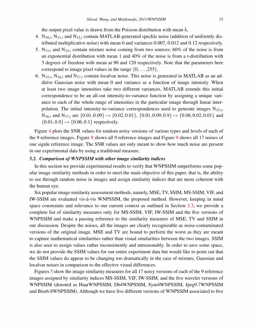
6. N15,i, N16,i and N17,i contain localvar noise. This noise is generated in MATLAB as an ad-ditive Gaussian noise with mean 0 and variance as a function of image intensity. Whenat least two image intensities take two different variances, MATLAB extends this initialcorrespondence to be an all-out intensity-to-variance function by assigning a unique vari-ance to each of the whole range of intensities in the particular image through linear inter-polation. The initial intensity-to-variance correspondences used to generate images N15,i,N16,i and N17,i are {0.01,0.09} 7→ {0.02,0.01}, {0.01,0.09,0.9} 7→ {0.08,0.02,0.01} and{0.01,0.9} 7→ {0.06,0.1} respectively.
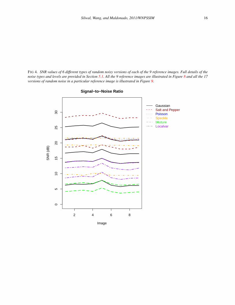
Figure 4 plots the SNR values for random noisy versions of various types and levels of each ofthe 9 reference images. Figure 8 shows all 9 reference images and Figure 9 shows all 17 noises ofone signle reference image. The SNR values are only meant to show how much noise are presentin our experimental data by using a traditional measure.
5.2. Comparison of WNPSSIM with other image similarity indicesIn this section we provide experimental results to verify that WNPSSIM outperforms some pop-
ular image similarity methods in order to meet the main objective of this paper, that is, the abilityto see through random noise in images and assign similarity indices that are more coherent withthe human eye.
Six popular image similarity assessment methods, namely, MSE, TV, SSIM, MS-SSIM, VIF, andIW-SSIM are evaluated vis-a-vis WNPSSIM, the proposed method. However, keeping in mindspace constraints and relevance to our current context as outlined in Section 3.3, we provide acomplete list of similarity measures only for MS-SSIM, VIF, IW-SSIM and the five versions ofWNPSSIM and make a passing reference to the similarity measures of MSE, TV and SSIM inour discussion. Despite the noises, all the images are clearly recognizable as noise-contaminatedversions of the original image. MSE and TV are bound to perform the worst as they are meantto capture mathematical similarities rather than visual similarities between the two images. SSIMis also seen to assign values rather inconsistently and unreasonably. In order to save some space,we do not provide the SSIM values for our entire experiment data but would like to point out thatthe SSIM values do appear to be changing too dramatically in the case of mixture, Gaussian andlocalvar noises in comparison to the effective visual differences.
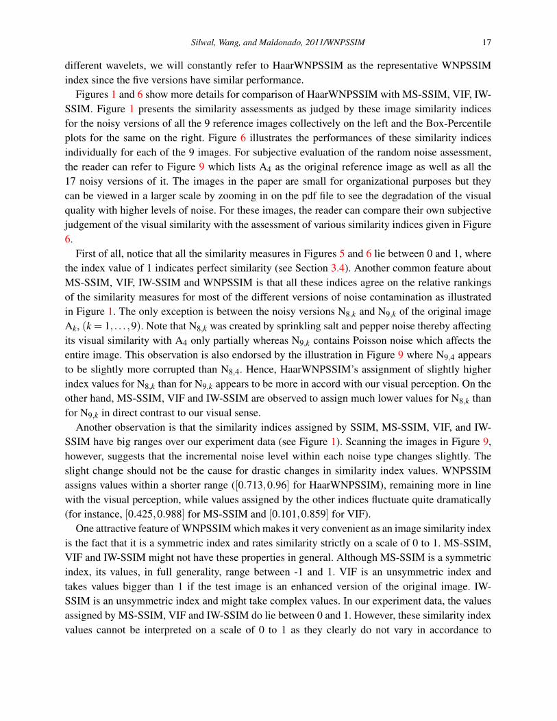
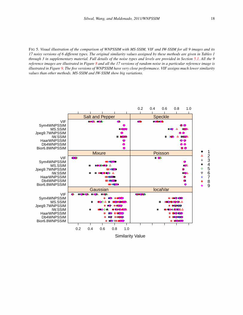
Figures 5 show the image similarity measures for all 17 noisy versions of each of the 9 referenceimages assigned by similarity indices MS-SSIM, VIF, IW-SSIM, and the five wavelet versions ofWNPSSIM (denoted as HaarWNPSSIM, Db4WNPSSIM, Sym4WNPSSIM, Jpeg9.7WNPSSIMand Bior6.8WNPSSIM). Although we have five different versions of WNPSSIM associated to five
Silwal, Wang, and Maldonado, 2011/WNPSSIM 16
FIG 4. SNR values of 6 different types of random noisy versions of each of the 9 reference images. Full details of thenoise types and levels are provided in Section 5.1. All the 9 reference images are illustrated in Figure 8 and all the 17versions of random noise in a particular reference image is illustrated in Figure 9.
2 4 6 8
05
1015
2025
30
Signal−to−Noise Ratio
Image
SN
R (
dB)
GaussianSalt and PepperPoissonSpeckleMixtureLocalvar
Silwal, Wang, and Maldonado, 2011/WNPSSIM 17
different wavelets, we will constantly refer to HaarWNPSSIM as the representative WNPSSIMindex since the five versions have similar performance.
Figures 1 and 6 show more details for comparison of HaarWNPSSIM with MS-SSIM, VIF, IW-SSIM. Figure 1 presents the similarity assessments as judged by these image similarity indicesfor the noisy versions of all the 9 reference images collectively on the left and the Box-Percentileplots for the same on the right. Figure 6 illustrates the performances of these similarity indicesindividually for each of the 9 images. For subjective evaluation of the random noise assessment,the reader can refer to Figure 9 which lists A4 as the original reference image as well as all the17 noisy versions of it. The images in the paper are small for organizational purposes but theycan be viewed in a larger scale by zooming in on the pdf file to see the degradation of the visualquality with higher levels of noise. For these images, the reader can compare their own subjectivejudgement of the visual similarity with the assessment of various similarity indices given in Figure6.
First of all, notice that all the similarity measures in Figures 5 and 6 lie between 0 and 1, wherethe index value of 1 indicates perfect similarity (see Section 3.4). Another common feature aboutMS-SSIM, VIF, IW-SSIM and WNPSSIM is that all these indices agree on the relative rankingsof the similarity measures for most of the different versions of noise contamination as illustratedin Figure 1. The only exception is between the noisy versions N8,k and N9,k of the original imageAk, (k = 1, . . . ,9). Note that N8,k was created by sprinkling salt and pepper noise thereby affectingits visual similarity with A4 only partially whereas N9,k contains Poisson noise which affects theentire image. This observation is also endorsed by the illustration in Figure 9 where N9,4 appearsto be slightly more corrupted than N8,4. Hence, HaarWNPSSIM’s assignment of slightly higherindex values for N8,k than for N9,k appears to be more in accord with our visual perception. On theother hand, MS-SSIM, VIF and IW-SSIM are observed to assign much lower values for N8,k thanfor N9,k in direct contrast to our visual sense.
Another observation is that the similarity indices assigned by SSIM, MS-SSIM, VIF, and IW-SSIM have big ranges over our experiment data (see Figure 1). Scanning the images in Figure 9,however, suggests that the incremental noise level within each noise type changes slightly. Theslight change should not be the cause for drastic changes in similarity index values. WNPSSIMassigns values within a shorter range ([0.713,0.96] for HaarWNPSSIM), remaining more in linewith the visual perception, while values assigned by the other indices fluctuate quite dramatically(for instance, [0.425,0.988] for MS-SSIM and [0.101,0.859] for VIF).
One attractive feature of WNPSSIM which makes it very convenient as an image similarity indexis the fact that it is a symmetric index and rates similarity strictly on a scale of 0 to 1. MS-SSIM,VIF and IW-SSIM might not have these properties in general. Although MS-SSIM is a symmetricindex, its values, in full generality, range between -1 and 1. VIF is an unsymmetric index andtakes values bigger than 1 if the test image is an enhanced version of the original image. IW-SSIM is an unsymmetric index and might take complex values. In our experiment data, the valuesassigned by MS-SSIM, VIF and IW-SSIM do lie between 0 and 1. However, these similarity indexvalues cannot be interpreted on a scale of 0 to 1 as they clearly do not vary in accordance to
Silwal, Wang, and Maldonado, 2011/WNPSSIM 18
FIG 5. Visual illustration of the comparison of WNPSSIM with MS-SSIM, VIF and IW-SSIM for all 9 images and its17 noisy versions of 6 different types. The original similarity values assigned by these methods are given in Tables 1through 3 in supplementary material. Full details of the noise types and levels are provided in Section 5.1. All the 9reference images are illustrated in Figure 8 and all the 17 versions of random noise in a particular reference image isillustrated in Figure 9. The five versions of WNPSSIM have very close performance. VIF assigns much lower similarityvalues than other methods. MS-SSIM and IW-SSIM show big variations.
Similarity Value
Bior6.8WNPSSIMDb4WNPSSIM
HaarWNPSSIMIW.SSIM
Jpeg9.7WNPSSIMMS.SSIM
Sym4WNPSSIMVIF
0.2 0.4 0.6 0.8 1.0
●●●●●
●●●●●
●●●●●
●●●●●
●●●●●
●●●●●
●●●●●
●●●●●
Gaussian
●●●
●●●
●●●
●●●
●●●
●●●
●●●
●●●
localVarBior6.8WNPSSIM
Db4WNPSSIMHaarWNPSSIM
IW.SSIMJpeg9.7WNPSSIM
MS.SSIMSym4WNPSSIM
VIF
●●
●●
●●
●●
●●
●●
●●
●●
Mixure
●
●
●
●
●
●
●
●
PoissonBior6.8WNPSSIM
Db4WNPSSIMHaarWNPSSIM
IW.SSIMJpeg9.7WNPSSIM
MS.SSIMSym4WNPSSIM
VIF
●●●
●●●
●●●
●●●
●●●
●●●
●●●
●●●
Salt and Pepper
0.2 0.4 0.6 0.8 1.0
●●●
●●●
●●●
●●●
●●●
●●●
●●●
●●●
Speckle
● 123456789
Silwal, Wang, and Maldonado, 2011/WNPSSIM 19
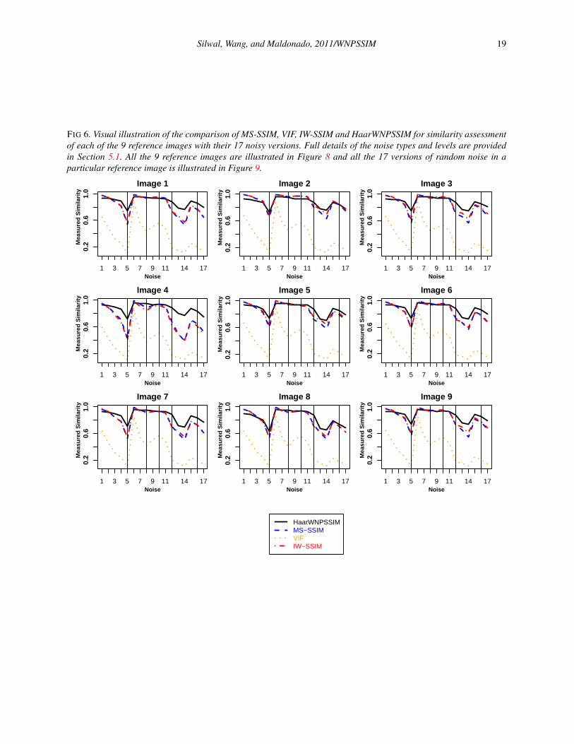
FIG 6. Visual illustration of the comparison of MS-SSIM, VIF, IW-SSIM and HaarWNPSSIM for similarity assessmentof each of the 9 reference images with their 17 noisy versions. Full details of the noise types and levels are providedin Section 5.1. All the 9 reference images are illustrated in Figure 8 and all the 17 versions of random noise in aparticular reference image is illustrated in Figure 9.
0.2
0.6
1.0
Mea
sure
d S
imila
rity
1 3 5 7 9 11 14 17
Image 1
Noise
0.2
0.6
1.0
Mea
sure
d S
imila
rity
1 3 5 7 9 11 14 17
Image 2
Noise
0.2
0.6
1.0
Mea
sure
d S
imila
rity
1 3 5 7 9 11 14 17
Image 3
Noise
0.2
0.6
1.0
Mea
sure
d S
imila
rity
1 3 5 7 9 11 14 17
Image 4
Noise
0.2
0.6
1.0
Mea
sure
d S
imila
rity
1 3 5 7 9 11 14 17
Image 5
Noise
0.2
0.6
1.0
Mea
sure
d S
imila
rity
1 3 5 7 9 11 14 17
Image 6
Noise
0.2
0.6
1.0
Mea
sure
d S
imila
rity
1 3 5 7 9 11 14 17
Image 7
Noise
0.2
0.6
1.0
Mea
sure
d S
imila
rity
1 3 5 7 9 11 14 17
Image 8
Noise
0.2
0.6
1.0
Mea
sure
d S
imila
rity
1 3 5 7 9 11 14 17
Image 9
Noise
HaarWNPSSIMMS−SSIMVIFIW−SSIM
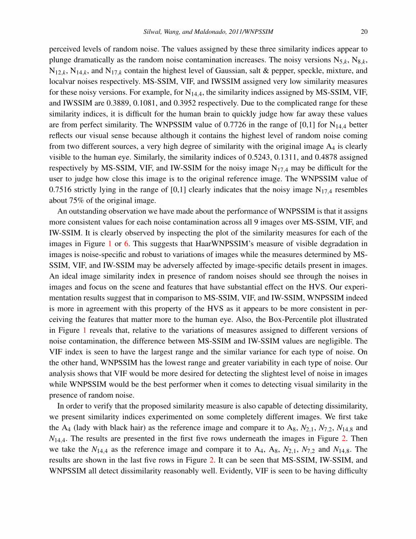
Silwal, Wang, and Maldonado, 2011/WNPSSIM 20
perceived levels of random noise. The values assigned by these three similarity indices appear toplunge dramatically as the random noise contamination increases. The noisy versions N5,k, N8,k,N12,k, N14,k, and N17,k contain the highest level of Gaussian, salt & pepper, speckle, mixture, andlocalvar noises respectively. MS-SSIM, VIF, and IWSSIM assigned very low similarity measuresfor these noisy versions. For example, for N14,4, the similarity indices assigned by MS-SSIM, VIF,and IWSSIM are 0.3889, 0.1081, and 0.3952 respectively. Due to the complicated range for thesesimilarity indices, it is difficult for the human brain to quickly judge how far away these valuesare from perfect similarity. The WNPSSIM value of 0.7726 in the range of [0,1] for N14,4 betterreflects our visual sense because although it contains the highest level of random noise comingfrom two different sources, a very high degree of similarity with the original image A4 is clearlyvisible to the human eye. Similarly, the similarity indices of 0.5243, 0.1311, and 0.4878 assignedrespectively by MS-SSIM, VIF, and IW-SSIM for the noisy image N17,4 may be difficult for theuser to judge how close this image is to the original reference image. The WNPSSIM value of0.7516 strictly lying in the range of [0,1] clearly indicates that the noisy image N17,4 resemblesabout 75% of the original image.
An outstanding observation we have made about the performance of WNPSSIM is that it assignsmore consistent values for each noise contamination across all 9 images over MS-SSIM, VIF, andIW-SSIM. It is clearly observed by inspecting the plot of the similarity measures for each of theimages in Figure 1 or 6. This suggests that HaarWNPSSIM’s measure of visible degradation inimages is noise-specific and robust to variations of images while the measures determined by MS-SSIM, VIF, and IW-SSIM may be adversely affected by image-specific details present in images.An ideal image similarity index in presence of random noises should see through the noises inimages and focus on the scene and features that have substantial effect on the HVS. Our experi-mentation results suggest that in comparison to MS-SSIM, VIF, and IW-SSIM, WNPSSIM indeedis more in agreement with this property of the HVS as it appears to be more consistent in per-ceiving the features that matter more to the human eye. Also, the Box-Percentile plot illustratedin Figure 1 reveals that, relative to the variations of measures assigned to different versions ofnoise contamination, the difference between MS-SSIM and IW-SSIM values are negligible. TheVIF index is seen to have the largest range and the similar variance for each type of noise. Onthe other hand, WNPSSIM has the lowest range and greater variability in each type of noise. Ouranalysis shows that VIF would be more desired for detecting the slightest level of noise in imageswhile WNPSSIM would be the best performer when it comes to detecting visual similarity in thepresence of random noise.
In order to verify that the proposed similarity measure is also capable of detecting dissimilarity,we present similarity indices experimented on some completely different images. We first takethe A4 (lady with black hair) as the reference image and compare it to A8, N2,1, N7,2, N14,8 andN14,4. The results are presented in the first five rows underneath the images in Figure 2. Thenwe take the N14,4 as the reference image and compare it to A4, A8, N2,1, N7,2 and N14,8. Theresults are shown in the last five rows in Figure 2. It can be seen that MS-SSIM, IW-SSIM, andWNPSSIM all detect dissimilarity reasonably well. Evidently, VIF is seen to be having difficulty
Silwal, Wang, and Maldonado, 2011/WNPSSIM 21
detecting dissimilarity between two images. Taking N14,4 (lady with the highest mixture noise) asthe reference image, the VIF index value for N14,8 (peppers with similar mixture noise) is 0.4396which is much higher than the VIF index is 0.0223 for A4 (noise-free version of N14,4 itself). TheHaarWNPSSIM index values for these comparisons are 0.1489 for the different image and 0.7726for the same image source. Clearly, HaarWNPSSIM is following the eye whereas VIF is merelycomparing the superficial noises rather than the underlying images, thus assigning a misleadinglyhigher similarity index.
Finally, although WNPSSIM has values much higher than the other ones for these dissimilaritycomparisons, it is to be noted that WNPSSIM is strictly on a scale of 0 to 1 while the othersare not. The non-parametric test we have employed in the construction of our similarity index isessentially an “iid” noise detector. Hence, our similarity index is not expected to perform wellin the case of some deterministic noises such as those caused by spatial filtering. In addition, alocally homogeneous region in one image compared to such a region in another image would givea non-rejection even though the two regions may represent different image contents or objects.Consequently, the cut-off threshold for unsimilarity for the entire images would shift upward awayfrom 0. The general rule of thumb is that if WNPSSIM is below 0.4, the images should be takento have significantly low structural similarity. This can be seen in our comparisons of completelydifferent images: A4 and N14,8, N14,4 and A8, and N14,4 and N7,2 in Figure 2, where WNPSSIMvalues are all between 0.25 and 0.4.
6. Applications and limitations of WNPSSIM
In this section, the applications and limitations of the proposed image similarity index, namely,WNPSSIM are described . We also discuss the question of whether or not WNPSSIM defines anactual distance.
6.1. Applications and limitations in image analysisAlgorithmic methods of image similarity assessment consistent with the HVS are most vigor-
ously pursued research topics in the image analysis literature. Robust methods, whether universalor context-specific, will evidently have huge applications in several fields as pointed out in Section1. In this article, a new image similarity assessment method by the name of WNPSSIM has beenproposed in the context of images contaminated with random noises from all possible sources. Im-ages are susceptible to random noise all too often such as during acquisition, storage and process-ing. Our experiments show that WNPSSIM is quite powerful in detecting visual similarity betweenimages when the images have been contaminated with random noises from various sources.
The construction of WNPSSIM we have described in this article worked out best for the exper-iments we have conducted which consisted of 9 standard 512× 512 test images common in theliterature. Some parameters in the construction of WNPSSIM can be adjusted in order to bettersuit the application data as follows:
1. Local window size: At typical viewing distances, only a local area in the image can be per-ceived with high resolution by the human observer at one time instance because of thefoveation feature of the HVS (Wang et al. [2004]). For this reason, computation of local
Silwal, Wang, and Maldonado, 2011/WNPSSIM 22
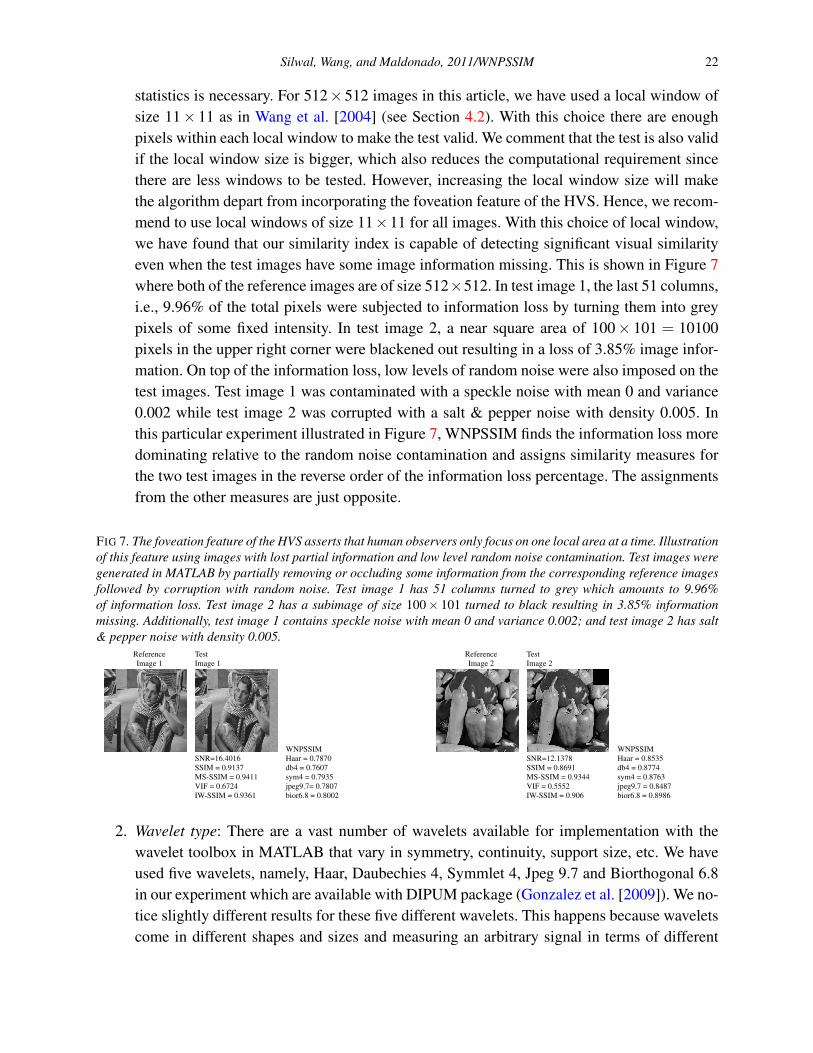
statistics is necessary. For 512×512 images in this article, we have used a local window ofsize 11× 11 as in Wang et al. [2004] (see Section 4.2). With this choice there are enoughpixels within each local window to make the test valid. We comment that the test is also validif the local window size is bigger, which also reduces the computational requirement sincethere are less windows to be tested. However, increasing the local window size will makethe algorithm depart from incorporating the foveation feature of the HVS. Hence, we recom-mend to use local windows of size 11×11 for all images. With this choice of local window,we have found that our similarity index is capable of detecting significant visual similarityeven when the test images have some image information missing. This is shown in Figure 7where both of the reference images are of size 512×512. In test image 1, the last 51 columns,i.e., 9.96% of the total pixels were subjected to information loss by turning them into greypixels of some fixed intensity. In test image 2, a near square area of 100× 101 = 10100pixels in the upper right corner were blackened out resulting in a loss of 3.85% image infor-mation. On top of the information loss, low levels of random noise were also imposed on thetest images. Test image 1 was contaminated with a speckle noise with mean 0 and variance0.002 while test image 2 was corrupted with a salt & pepper noise with density 0.005. Inthis particular experiment illustrated in Figure 7, WNPSSIM finds the information loss moredominating relative to the random noise contamination and assigns similarity measures forthe two test images in the reverse order of the information loss percentage. The assignmentsfrom the other measures are just opposite.
FIG 7. The foveation feature of the HVS asserts that human observers only focus on one local area at a time. Illustrationof this feature using images with lost partial information and low level random noise contamination. Test images weregenerated in MATLAB by partially removing or occluding some information from the corresponding reference imagesfollowed by corruption with random noise. Test image 1 has 51 columns turned to grey which amounts to 9.96%of information loss. Test image 2 has a subimage of size 100× 101 turned to black resulting in 3.85% informationmissing. Additionally, test image 1 contains speckle noise with mean 0 and variance 0.002; and test image 2 has salt& pepper noise with density 0.005.
Reference Test Reference TestImage 1 Image 1 Image 2 Image 2
WNPSSIM WNPSSIMSNR=16.4016 Haar = 0.7870 SNR=12.1378 Haar = 0.8535SSIM = 0.9137 db4 = 0.7607 SSIM = 0.8691 db4 = 0.8774MS-SSIM = 0.9411 sym4 = 0.7935 MS-SSIM = 0.9344 sym4 = 0.8763VIF = 0.6724 jpeg9.7= 0.7807 VIF = 0.5552 jpeg9.7 = 0.8487IW-SSIM = 0.9361 bior6.8 = 0.8002 IW-SSIM = 0.906 bior6.8 = 0.8986
2. Wavelet type: There are a vast number of wavelets available for implementation with thewavelet toolbox in MATLAB that vary in symmetry, continuity, support size, etc. We haveused five wavelets, namely, Haar, Daubechies 4, Symmlet 4, Jpeg 9.7 and Biorthogonal 6.8in our experiment which are available with DIPUM package (Gonzalez et al. [2009]). We no-tice slightly different results for these five different wavelets. This happens because waveletscome in different shapes and sizes and measuring an arbitrary signal in terms of different
Silwal, Wang, and Maldonado, 2011/WNPSSIM 23
wavelets will produce different results. In fact, it is possible to find empirically a waveletthat works best for a given data set of images, such as faces, fingerprints, terrain, paintings,etc. For example, for a data set of aerial images of skyscrapers, Haar wavelets will providethe best succinct representation with least wavelet coefficients due to their block-like resem-blance. However, we notice for our collection of experimental images, WNPSSIM basedon the selected five wavelets produce similar measures and that they all perform better incomparison with the other image quality assessment methods considered in this article. Ifthe application data set is not well-defined, we recommend using Haar wavelets for theirsimplicity.
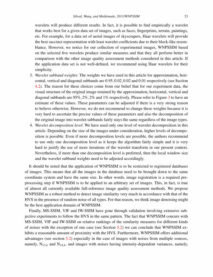
3. Wavelet subband weights: The weights we have used in this article for approximation, hori-zontal, vertical and diagonal subbands are 0.95,0.02,0.02 and 0.01 respectively (see Section4.2). The reason for these choices come from our belief that for our experiment data, thevisual structure of the original image retained by the approximation, horizontal, vertical anddiagonal subbands are 95%,2%,2% and 1% respectively. Please refer to Figure 3 to have anestimate of these values. These parameters can be adjusted if there is a very strong reasonto believe otherwise. However, we do not recommend to change these weights because it isvery hard to ascertain the precise values of these parameters and also the decomposition ofthe original image into wavelet subbands fairly stays the same regardless of the image types.
4. Wavelet decomposition level: We have used only one level of wavelet decomposition in thisarticle. Depending on the size of the images under consideration, higher levels of decompo-sition is possible. Even if more decomposition levels are possible, the authors recommendto use only one decomposition level as it keeps the algorithm fairly simple and it is veryhard to justify the use of more iterations of the wavelet transform in our present context.Nevertheless, if more than one decomposition level is preferred, then the local window sizeand the wavelet subband weights need to be adjusted accordingly.
It should be noted that the application of WNPSSIM is to be restricted to registered databasesof images. This means that all the images in the database need to be brought down to the samecoordinate system and have the same size. In other words, image registration is a required pre-processing step if WNPSSIM is to be applied to an arbitrary set of images. This, in fact, is trueof almost all currently available full-reference image quality assessment methods. We proposeWNPSSIM as a robust method to detect image similarity very much in accordance with that of theHVS in the presence of random noise of all types. For that reason, we think image denoising mightbe the best application domain of WNPSSIM.
Finally, MS-SSIM, VIF and IW-SSIM have gone through validation involving extensive sub-jective experiments to follow the HVS in the same pattern. The fact that WNPSSIM concurs withMS-SSIM, VIF and IW-SSIM on relative rankings of the similarity measures for different kindsof noises with the exception of one case (see Section 5.2) we can conclude that WNPSSIM ex-hibits a reasonable amount of proximity with the HVS. Furthermore, WNPSSIM offers additionaladvantages (see section 5.2) especially in the case of images with noises from multiple sources,namely, N13,k and N14,k, and images with noises having intensity-dependent variances, namely,
Silwal, Wang, and Maldonado, 2011/WNPSSIM 24
N15,k through N17,k.The authors are aware that there are some large-scale image databases featuring psycho-visual
experimentation such as LIVE image quality assessment database (Sheikh et al. [2005b]) andTID2008 database (Ponomarenko et al. [2009b]) available for use completely free of charge toresearchers. However, the main purpose in this paper is the detection of visual similarity betweenimages degraded only through random noise contamination. Deterministic noises such as com-pression and blurring are beyond the scope of this paper. In order to establish the robustness ofthe proposed method, we need several different kinds of random noises at several different levels.Most publicly available databases, featuring both deterministic and random noises, are speciallydesigned for universal image similarity assessment methods. However, due to an insufficient num-ber of variations in random noise, they are not quite suitable to serve the specific purpose under-taken in this paper. This is essentially what prompted us to come up with our own experimentdata. The authors were unable to locate any publicly available databases which offered the varietyof random noises we have considered in this paper. For example, our experiment data features amixture noise which is a random noise with more than one source. A mixture noise is certainly arealistic noise since images in real life subjected to various processes are susceptible to contami-nation from multiple sources. Our experiments show that this type of noise might adversely affectthe performance of some popular image similarity indices such as SSIM. Also, the results in thecontext of the 5 relatively complicated noises N13,k through N17,k sufficiently convince the authorsto refrain from resorting to any large-scale experiments. In light of the large proportion of time andeffort such experimentation would require as well as its value in its own right, the authors wish toundertake it as a separate project in the future.
6.2. Does WNPSSIM define a distance?It is relevant to raise a question as to whether or not WNPSSIM defines a distance. We give a
negative answer to this question and provide an argument that a distance as an image similarityassessment method is not necessarily desirable. A distance is usually desired for its mathematicalconvenience due to the fact that it makes a continuous measurement of distances between im-ages possible. A distance d, by definition, is a function taking values in [0,∞) and possessing thefollowing properties:
1. d(X ,Y ) = d(Y,X) for any two images X and Y .2. d(X ,Y ) = 0 if and only if the two images X and Y are identical.3. d(X ,Y )≤ d(X ,Z)+d(Z,Y ) for any three images X ,Y and Z.
To a distance, an M×N matrix is just a mathematical point in the space RMN and it treats all thepoints in this space exactly the same way without any discrimination. Consequently, a distancelacks the ability to take into account the redundancy present in natural images as it cannot dis-tinguish between random matrices and matrices corresponding to natural images. However, as wehave remarked in Section 1, the whole purpose of image quality assessment is to provide a methodthat goes hand in hand with the HVS in determining the proximity between the natural images. Adistance in the space of all possible images (random and natural), clearly, will not do justice to the
Silwal, Wang, and Maldonado, 2011/WNPSSIM 25
set of natural images which, according to the discussion in Section 4.1, is merely a thin subset ofthe space of all images and, therefore, cannot be the right tool for image quality assessment.
Given the range and meaning of WNPSSIM (i.e., the interval [0,1], with 0 indicating completedissimilarity and 1 complete similarity), a natural candidate for a distance defined by WNPSSIMis d(X ,Y ) = −log(WNPSSIM(X ,Y )), which trivially verifies Properties 1 and 2. Along the linesof the previous discussion, the fact that d(X ,Y ) fails to satisfy Property 3 will attest to its abilityto discriminate between natural images and mathematical matrices. This is indeed the case, forinstance, if we consider X =A4, Y =A8 and Z =N14,4, where the images A4, A8, and N14,4 are asin Figure 2. Then we find from the WNPSSIM values in the same figure,
7.6009 = d(X ,Y )≥ d(Z,Y )+d(X ,Z) = 1.3556+0.2580.
Hence, as anticipated, d does not satisfy Property 3. In addition, the corresponding values ofd(X ,Y ), d(Z,Y ), and d(X ,Z) are in accordance with visual perception. Meaning, images X andY are clearly different images, Z is a noisy version of X and our assessment of its distance to X andY is hindered by the existence of noises leading to smaller distances.
7. Conclusion
One of the properties of the HVS is the ability to see through a low-level of random noisecontamination and recognize the underlying image. Another important property of the HVS is itsmulti-channel parallel pathways (see Section 4.1). This article seeks to emulate these two proper-ties in the proposed image similarity index.
In this article, we have developed an image similarity index WNPSSIM that provides a mea-sure of visual similarity on a scale of 0 to 1 between any two supplied images. In practice, oneof the images is a reference image and the other one is a random-noisy version of it and the goalis to assess the similarity between the two, incorporating the seeing-through ability of moderatelevels of random noise in images. The main idea of the construction of WNPSSIM is to applya non-parametric test to the relative difference of the reference image and the test image in thewavelet domain to evaluate the structural similarity of the images locally. The final similarity as-sessment method integrates the information from the level-one wavelet subbands as well as thelocal luminance comparison.
Since the WNPSSIM index is a method based on multi-scale decomposition techniques, the threeother multi-scale similarity indices, MS-SSIM, VIF, and IW-SSIM, have presented themselvesas suitable choices for comparison against the performance of WNPSSIM in the present contextof this article. Furthermore, these three similarity indices are extensively tested methods and arewidely regarded as state-of-the-art performers in mimicking the human visual system (HVS). Ourexperimentation show that WNPSSIM indeed shares the virtues of MS-SSIM, VIF, IW-SSIM indetecting visual similarity between images very much in sync with the HVS. This is clear from thefact that MS-SSIM, VIF, IW-SSIM, and WNPSSIM almost always agree on the rankings of differ-ent types of noisy versions according to their visual similarity with the reference image. Our resultsfind that WNPSSIM offers additional advantage over the other considered image similarity indiceswhen it comes to random-noise contamination. WNPSSIM values comply more with our visual
Silwal, Wang, and Maldonado, 2011/WNPSSIM 26
sense by assigning similarity values using the geometric mean of the proportions of local agree-ments between the two images in each wavelet subband scaled by the average luminance. Further,slight incremental changes in the levels of noise seem to affect the images in our experiment dataonly slightly in terms of visual degradation. This fact is reflected very well in WNPSSIM values.The other similarity indices, on the other hand, show drastic changes in their values for these noisyimages. Since various kinds of random noises inevitably exist in abundance in digital images, anon-parametric image quality assessment method as the one proposed in this article should haveplenty of potential to provide a reliable similarity measure in this context.
Acknowledgements
This work was partially supported by a grant from the National Science Foundation (DMS0901587 to Diego Maldonado) and a grant from the Simons Foundation (#246077 to HaiyanWang).
References
Bovik, A. (2009). The Essential Guide to Image Processing. Academic Press.Chandler, D. M. and Hemami, S. S. (2005). Dynamic contrast-based quantization for lossy wavelet
image compression. IEEE T. Image Process., 14(4):397–410.Chandler, D. M. and Hemami, S. S. (2007). A wavelet-based visual signal-to-noise ratio for natural
images. IEEE T. Image Process., 16(9):2284–2298.Daubechies, I. (1992). Ten lectures on wavelets. Society for Industrial and Applied Mathematics.Donoho, D. L. (1995). Denoising via wavelet shrinkage. IEEE T. Inform. Theory, 41(3):613–627.Donoho, D. L. and Johnstone, I. M. (1994). Ideal spatial adaptation by wavelet shrinkage.
Biometrika, 81(3):425–455.Egiazarian, K., Astola, J., Ponomarenko, N., Lukin, V., Battisi, F., and Carli, M. (2006). New full-
reference quality metrics based on HVS. CD-ROM Proceedings of the Second Int. Workshop onVideo Proc. and Quality Metrics.
Field, D. J. (1987). Relations between the statistics of natural images and the response propertiesof cortical cells. J. Opt. Soc. Am., 4(12):2379–2394.
Field, D. J. (1999). Wavelets, vision and the statistics of natural scenes. Philosophical Transactionsof the Royal Society: Mathematical, Physical and Engineering Sciences, 357(1760):2527–2542.
Field, D. J. and Brady, N. (December 1997). Visual sensitivity, blur and the sources of variabilityin the amplitude spectra of natural scenes. Vision Res., 37(23):3367–3383.
Gagnon, L. and Jouan, A. (1997). Speckle filtering of SAR images - a comparative study betweencomplex-wavelet based and standard filters. Proc. SPIE, 3169:80–91.
Gao, X., Lu, W., Tao, D., and Li, X. (2009). Image quality assessment based on multiscale geo-metric analysis. IEEE T. Image Process., 18(7):1409–1423.
Gao, X., Lu, W., Tao, D., and Li, X. (2010). Image quality assessment and human visual system.Proc. SPIE, 7744:77440Z.
Gonzalez, R., Woods, R., and Eddins, S. (2009). Digital Image Processing Using Matlab. Gates-mark Publishing.
Silwal, Wang, and Maldonado, 2011/WNPSSIM 27
Huang, J. and Mumford, D. (1999). Statistics of natural images and models. Computer Vision andPattern Recognition, 1:1541–1547.
Kim, M. H. and Akritas, M. G. (2010). Order thresholding. Ann. Stat., 38(4):2314–2350.Lai, Y.-K. and Kuo, C.-C. J. (2000). A Haar wavelet approach to compressed image quality as-
sessment. J. Vis. Commun. Image R., 11:17–40.Luisier, F., Vonesch, C., Blu, T., and Unser, M. (2010). Fast interscale wavelet denoising of
poisson-corrupted images. Signal Process., 90(2):415–427.Mallat, S. G. (2008). A Wavelet Tour of Signal Processing: the Sparse Way. Academic press, 3rd
edition.Mallat, S. G. (July 1989). A theory for multiresolution signal decomposition: The wavelet repre-
sentation. IEEE T. Pattern Anal., 2(7):674–693.Millane, R. P., Alzaidi, S., and Hsiao, W. H. (2003). Scaling and power spectra of natural images.
Image Vision Comput., 14(12):2117–2128. Palmerston North, NZ.Ninassi, A., Meur, O. L., Callet, P. L., and Barba, D. (2008). On the performance of human visual
system based image quality assessment metric using wavelet domain. Proc. SPIE Human Visionand Electronic Imaging XIII, (6806).
Ninassi, A., Meur, O. L., Callet, P. L., Barba, D., and Tirel, A. (2006). Task impact on the visualattention in subjective image quality assessment. Proc. SPIE 14th European Signal Process.Conf. Florence, Italy.
Ponomarenko, N., Battisti, F., Egiazarian, K., Astola, J., and Lukin, V. (Jan 2009a). Metrics perfor-mance comparison for color image database. 4th Intl. Workshop Video Process. Quality MetricsConsumer Electron., (6):6.
Ponomarenko, N., Lukin, V., Zelensky, A., Egiazarian, K., Carli, M., and Battisti, F. (2009b).TID2008 - a database for evaluation of full-reference visual quality assessment metrics. Ad-vances of Modern Radioelectronics, 10.
Portilla, J., Strela, V., Wainwright, M. J., and Simoncelli, E. P. (2003). Image denoising using scalemixtures of Gaussians in the wavelet domain. IEEE T. Image Process., 12(11):1338–1351.
Richter, T. and Larabi, C. (2008). Toward objective image quality metrics: the AIC Eval Programof the JPEG. Proc. of SPIE, 7073(1):70730X. doi:10.1117/12.795096.
Ruderman, D. L. (1997). Origins of scaling in natural images. Vision Res., 37(23):3385–3398.Sheikh, H. R. and Bovik, A. C. (2006). Image information and visual quality. IEEE T. Image
Process., 15(2):430–444.Sheikh, H. R., Bovik, A. C., and de Veciana, G. (2005a). An information fidelity criterion for image
quality assessment using natural scene statistics. IEEE T. Image Process., 14(12):2117–2128.Sheikh, H. R., Wang, Z., Cormack, L., and Bovik, A. C. (2005b). LIVE image quality assessment
database, release 2, available at http://live.ece.utexas.edu/research/quality.Simoncelli, E. P. and Adelson, E. H. (1996). Noise removal via bayesian wavelet coring. IEEE T.
Image Process., 14(12):2117–2128.Tolhurst, D. J., Tadmor, Y., and Chao, T. (1992). Amplitude spectra of natural images. Ophthalm.
Physiol. Opt., 12(2):229–232.
Silwal, Wang, and Maldonado, 2011/WNPSSIM 28
Vonesch, C., Aguet, F., Vonesch, J., and Unser, M. (2006). The colored revolution of bioimaging.IEEE Signal Process. Mag., 3:20–31.
Wainwright, M. J., Simoncelli, E. P., and Wilsky, A. S. (2001). Random cascades on wavelettrees and their use in analyzing and modeling natural images. Appl. Comput. Harmon. Anal.,11:89–123.
Wang, H. and Akritas, M. G. (2004). Rank tests for ANOVA with large number of factor levels. J.Nonparametr. Stat., 16(3-4):563–589.
Wang, H., Maldonado, D., and Silwal, S. (2011). A nonparametric-test-based structural similaritymeasure for digital images. Comput. Stat. Data. An., 55(11):2925–2936.
Wang, H., Neill, J., and Miller, F. (2008). Nonparametric clustering of functional data. Statisticsand its Interface, 1:47–62.
Wang, H., Tolos, S., and Wang, S. (2010). A distribution-free nonparametric test to detect de-pendence between a response variable and covariate in presence of heteroscedastic treatmenteffects. Can. J. Stat., 38(3):408–433.
Wang, Z. and Bovik, A. (2002). A universal image quality index. IEEE Signal Proc. Let., 9(3):81–84.
Wang, Z., Bovik, A., Sheikh, H., and Simoncelli, E. (2004). Image quality assessment: From errorvisibility to structural similarity. IEEE T. Image Process., 13(4):600–612.
Wang, Z. and Bovik, A. C. (2009). Mean squared error: Love it or leave it? A new look at signalfidelity measures. IEEE Signal. Proc. Mag., 26(1):98–117.
Wang, Z. and Li, Q. (2011). Information content weighting for perceptual image quality assess-ment. IEEE T. Image Process., 20(5):1185–1198.
Wang, Z. and Simoncelli, E. P. (2005a). Reduced-reference image quality assessment using awavelet-domain natural image statistic model. Proc. of SPIE Human Vision and ElectronicImaging, 5666:149–159.
Wang, Z. and Simoncelli, E. P. (2005b). Translation insensitive image similarity in complexwavelet domain. Proc. IEEE Inter. Conf. Acoustic, Speech and Signal Proc., 2:573–576.
Wang, Z., Simoncelli, E. P., and Bovik, A. C. (Nov. 2003). Multi-scale structural similarity forimage quality assessment. Proc. 37th IEEE Asilomar Conf. on Signals, Systems, and Computers.
Watanabe, A., Mori, T., Nagata, S., and Hiwatashi, K. (1968). Spatial sine-wave responses of thehuman visual system. Vision Res., 8:1245–1263.
Watson, A. B. (1987). The cortex transform: Rapid computation of simulated neural images.Comput. Vis. Graph. Image Process., 39:311–327.
Xiong, Z., Ramchandran, K., and Orchard, M. T. (1997). Space-frequency quantization for waveletimage coding. IEEE T. Image Process., 6:677–693.
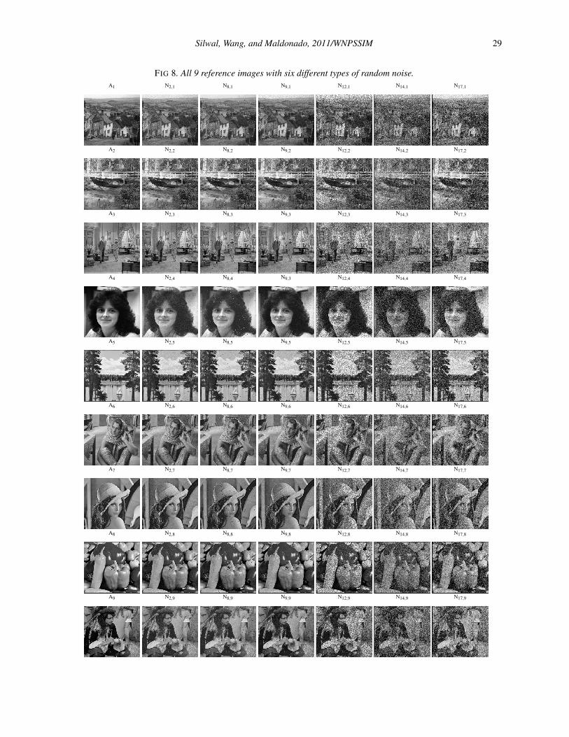
Silwal, Wang, and Maldonado, 2011/WNPSSIM 29
FIG 8. All 9 reference images with six different types of random noise.A1 N2,1 N8,1 N9,1 N12,1 N14,1 N17,1
A2 N2,2 N8,2 N9,2 N12,2 N14,2 N17,2
A3 N2,3 N8,3 N9,3 N12,3 N14,3 N17,3
A4 N2,4 N8,4 N9,3 N12,4 N14,4 N17,4
A5 N2,5 N8,5 N9,5 N12,5 N14,5 N17,5
A6 N2,6 N8,6 N9,6 N12,6 N14,6 N17,6
A7 N2,7 N8,7 N9,7 N12,7 N14,7 N17,7
A8 N2,8 N8,8 N9,8 N12,8 N14,8 N17,8
A9 N2,9 N8,9 N9,9 N12,9 N14,9 N17,9
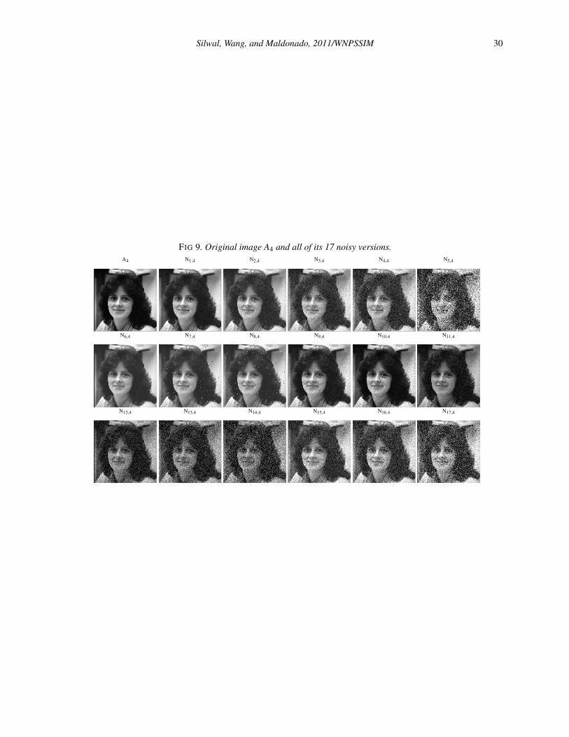
Silwal, Wang, and Maldonado, 2011/WNPSSIM 30
FIG 9. Original image A4 and all of its 17 noisy versions.A4 N1,4 N2,4 N3,4 N4,4 N5,4
N6,4 N7,4 N8,4 N9,4 N10,4 N11,4
N12,4 N13,4 N14,4 N15,4 N16,4 N17,4