WORKING PAPERS

R&D in Trade Networks: The Role of Asymmetry

Mariya Teteryatnikova

January 2016

Working Paper No: 1601

DEPARTMENT OF ECONOMICS

UNIVERSITY OF VIENNA

All our working papers are available at: http://mailbox.univie.ac.at/papers.econ

R&D in Trade Networks: The Role of Asymmetry∗

Mariya Teteryatnikova†

University of Vienna

January 15, 2015

Abstract

Countries differ substantially in their exposure to international trade as determined by thenumber of their trade partners. This exposure to trade and the asymmetry in trade exposure areanticipated by firms when making their R&D investments. We model a choice of R&D investmentsby firms in a given trade network focusing on the effects of the network asymmetry. The twolarge classes of networks considered include asymmetric hub-and-spoke networks and symmetricnetworks. We find that R&D, productivity and welfare are highest in a hub economy and lowestin a spoke, and the larger the degree of network asymmetry, the larger the difference. A countryin a symmetric network exhibits intermediate levels of R&D and welfare, even if the number of itstrade partners is the same as in a hub or in a spoke. This implies that regional/preferential tradeagreements, which result in a highly asymmetric trade network, benefit hub economies but harmspokes. By contrast, multilateral trade agreements, which lead to a symmetric complete network,generate equal R&D and welfare benefits for all countries.

JEL Classification: O31, D85, D43, L13, F13

Keywords: Trade, hub-and-spoke network, asymmetry, R&D, oligopolistic competition

∗I would like to thank Morten Ravn, Fernando Vega-Redondo, Yves Zenou, Peter Neary, Andrea Galeotti, Francis Bloch, Juan

M. Ruiz, Christian Ghiglino, Andrey Levchenko, and my current and former colleagues at the University of Vienna, especially

Maarten Janssen, Karl Schlag, Alejandro Cunat, Harald Fadinger, Daniel Garcia, Marc Goni, Wieland Muller and Christian

Roessler, for helpful comments and feedback. I also thank the research staff of the WTO, especially Michele Ruta, Patrick

Low and Roberta Piermartini, and participants of various conferences and seminars where this paper (in its earlier and cur-

rent versions) was presented, including University of Vienna, University of Oxford, University of Nottingham, Essex University,

Wirtschaftsuniversitat Wien, Bank of England, Institute for Advanced Studies (IHS), CORE, Johns Hopkins Center (Bologna),

IMT Institute for Advanced Studies, EEA, SAET, Simposio de la Asociacion Espanola de Economia, International Conference

on the Formation and the Evolution of Social and Economic Networks, and ELSNIT.†University of Vienna, Department of Economics, Oskar-Morgenstern-Platz 1, 1090 Vienna, Austria, phone: +43-1-4277-37427,

e-mail: mariya.teteryatnikova@univie.ac.at

1 Introduction

The last three decades of globalization, expansion of the World Trade Organization (WTO) and un-

precedented spread of preferential trade agreements between countries have resulted in international

trade network turning progressively large and complex. One of its key features is large asymmetries

in countries’ exposure to international trade, where some countries trade with many foreign partners,

while others trade with only a few.1 The main message of this paper is that this asymmetry in coun-

tries’ trade exposure is an important determinant of firms’ innovation, productivity and countries’

welfare. It benefits countries that trade with many other countries but harms those that trade with

a few.

This message has a number of relevant implications. First, it suggests that disregarding asymme-

try of the trade system may lead to biased empirical estimates of the impact of trade on innovation,

productivity, welfare and – in the long run – on countries’ economic growth. This bias is already

anticipated by empirical research that emphasizes the importance of trade network topology and

country’s position in the network for the country’s economic growth and trade benefits (Kali and

Reyes, 2007; Yang and Gupta, 2005). Secondly, it implies that firms’ innovation incentives and

productivity as well as countries’ welfare depend on the type of their trade agreements with other

countries – multilateral or preferential/regional – since each type of trade agreements is associated

with a specific type of countries’ trade involvement in the overall network of trade. The comparison

of multilateral and regional trade agreements in terms of firms’ productivity and countries’ welfare

offers new insights into the reasons for proliferation of regional trade agreements and simultaneous

stagnation of multilateral trade talks within the WTO.2 It also provides a new viewpoint on the ques-

tion that has attracted much attention in recent public debates and trade policy research on whether

allowing for regional trade agreements in the WTO (Article XXIV of the General Agreement on

Trade and Tariffs (GATT)) helps or hinders the ultimate goal of multilateral free trade. Finally, by

bringing the main message of the paper to the context of inter-regional trade within one country, we

obtain that asymmetry in inter-regional trade relations may be an important factor contributing to

the commonly observed disparities in firms’ productivity and wealth across regions.3

The effects of trade on firms’ innovation and endogenous productivity growth has been a subject of

extensive research in trade literature. In particular, recent empirical studies find that trade openness

1In the literature, the international trade network is often described as core-periphery or hub-and-spoke in structure.Early discussion of hub-and-spoke trade systems can be found in Wonnacott (1990, 1991, 1996) and Kowalczyk andWonnacott (1992). More recent studies include Baldwin (2004), Yang and Gupta (2005), De Benedictis et al. (2005),Deltas et al. (2006), Horaguchi (2007), Chong and Hur (2008), Kali and Reyes (2007), Fagiolo et al. (2009).

2The WTO online statistics asserts that “regional trade agreements (RTAs) have become increasingly prevalentsince the early 1990s. As of 31 July 2013, some 575 notifications of RTAs ... had been received by the GATT/WTO.”(www.wto.org/english/tratop e/region e/region e.htm.) Figure 4 in the Appendix demonstrates this development.At the same time, multilateral trade negotiations have stalled soon after the launch of the Doha Development Roundin Qatar in 2001, with most significant disagreement being between the group of developed and developing nations.For details see, for example, Schott (2004), Fergusson (2008, 2011), and Bhagwati (2012).

3Strong wealth polarization exists in many countries. For example, according to the statistics reported by TheEconomist (March 10th, 2011), Britain and the U.S.A. have the widest regional disparities in a group of developedcountries covered by the survey. Average GDP per head in central London is more than nine times larger than in partsof Wales; and the District of Columbia in the U.S. is five times as rich as Mississippi. Italy and Germany have thesmallest regional spread, yet incomes in their most affluent areas are still almost three times those of the poorest.

1

increases firms’ incentives to innovate and adopt new technologies. For example, Verhoogen (2008)

reports that Mexican exporting firms are more likely than non-exporters to be ISO 9000 certified,

which is a proxy for the use of more advanced production techniques; and Bustos (2011) finds

that Mercosur trade agreement generated an increase in new technology spending by Argentinian

exporters.4 Complementary to empirical work, theoretical studies substantiate the predominantly

positive effects of trade on firms’ R&D and productivity and identify various channels for these

effects. Traditionally, most of these studies analyze the setting with just two countries, home and

foreign, or offer numerical results for the setting with more than two countries.

In this paper, we propose an analytical framework with multiple countries to examine how the

impact of trade on firms’ R&D and productivity depends on structural features of the trade network.

We focus on the effects of asymmetry in the number of countries’ trade partners. The key idea is that

asymmetry in trade relations creates heterogeneity in aggregate demand faced by firms in different

countries, which in turn, leads to different incentives for innovation.

We develop this idea in a model where trade relations between countries are represented by a

network. Nodes of the network are countries and links indicate trade agreements or other regulations

that allow trade between the linked countries. Given the focus of the paper on the role of trade

network asymmetry, we consider the countries as identical in all but their position in the network.

In such setting the network formation models of Goyal and Joshi (2006), Furusawa and Konishi

(2007) and Mauleon et al. (2010) have shown that asymmetries in countries’ trade relations cannot

emerge endogenously. Therefore, for the purposes of our analysis here we regard the trade network

as exogenous but derive comparative static effects of a change in the relative number of country’s

trade partners on firms’ innovation and countries’ welfare.5

The structure of the trade network determines the degree of country’s trade exposure, that is, the

number of foreign markets it has access to and the level of competition in every market. Building on

the studies of trade agreements in oligopoly setting (Goyal and Joshi, 2006; Saggi, 2006; Chen and

Joshi, 2010), we consider Cournot competition between firms in every market and the intra-industry

type of trade.6 For simplicity we also assume that there is a single home producer in each country

that can sell its good in the domestic market and in the markets of its trade partner countries.

As a result, a firm in the country that has many trade links with other countries is likely to face

larger aggregate demand for its good than a firm in the country that has only a few links. On the

other hand, it also faces higher competition, at least in the domestic market. The ultimate size of

firm’s demand is determined by both, the number of its trade links and the level of competition in

its domestic and foreign markets, where the latter, in turn, is defined by the number of the foreign

4Similar patterns in firm innovation and productivity improvement are shown by Lileeva and Trefler (2010) forCanada, Bernard et al. (2006, 2007) for the U. S., Topalova (2004) for India, Aw et al. (2000) for Korea and Taiwan,Alvarez and Lopez (2005) for Chile, De Loecker (2007) for Slovenia, and Van Biesebroeck (2005) for sub-Saharan Africa.

5In the conclusion we discuss a possibility of endogenous formation of asymmetric networks in a model that allowsfor cross-country differences in firms’ demand and cost structure.

6We opt for oligopolistic competition, rather than monopolistic competition, which is more commonly assumed ininternational trade theory, since process R&D merges better with Brander (1981) oligopoly model than with Krugman(1980) monopolistic competition model.

2

markets’ own links. This suggests that asymmetry in the pattern of trade relations between countries

is likely to create heterogeneity among firms in terms of their aggregate demand.

The aggregate demand heterogeneity then becomes a key reason for the difference in firms’ incen-

tives to innovate. This follows from the interaction between the size of aggregate demand, increasing

returns and R&D investment. Before competing in a product market, firms can perform cost-reducing

innovations, or process R&D. Using the modeling assumptions of D’Aspremont and Jacquemin (1988)

and Goyal and Moraga (2001), we consider the cost of R&D to be fixed, that is, independent of the

amount produced, while the returns to R&D to be larger the larger the aggregate demand.7 As a

result and consistently with much empirical evidence (Griliches, 1957; Gustavsson, 1999; Kremer,

2002; Acemoglu and Linn, 2004), firm’s incentives to innovate increase in its aggregate demand. Then

in asymmetric trade networks, where aggregate demand of a firm depends on its network position,

the incentives to innovate may differ substantially across firms. The difference in firms’ R&D invest-

ments, in turn, translates into their productivity differences and eventually generates a disparity in

countries’ welfare.

We consider two large classes of trade network structures. In the spotlight of our analysis is the

class of asymmetric, hub-and-spoke or core-periphery type of networks, where some countries (hubs)

have a relatively large number of trade partners whereas other countries (spokes) have only a few

partners. In the literature, such hub-and-spoke type of structure is considered to be a close fit to

the actual international trade network, both in overall terms and at the commodity-specific level.8

Within this class of networks we allow for a variation in the share of hubs and spokes among trade

partners of a given country. For simplicity, we focus on networks where all hub nodes are the same

and all spoke nodes are the same, so that each network can be characterized by just four parameters:

the number of trade partners of a hub, number of trade partners of a spoke, share of hubs among

trade partners of a hub, and share of spokes among trade partners of a spoke. A variation in the

first two parameters allows addressing the effects of asymmetry in countries’ trade involvement. In

addition, a variation in the last two allows studying the effects of the exact pattern of asymmetry. The

latter means that we can analyze how for a given degree of asymmetry, the composition of countries’

trade partners, and thus the extent of their own trade involvement, matter for firms’ incentives to

innovate.9 The results of our analysis for the hub-and-spoke type of networks are then compared

with those for the class of symmetric, or regular structures. In a symmetric network all countries

have the same number of trade partners, and the special case where any country is linked to every

other country is referred to as the complete network.

The primary result of this paper is that the impact of trade on firm’s R&D and productivity

7In contrast to D’Aspremont and Jacquemin (1988) and Goyal and Moraga (2001), the focus of this paper is onthe effects on R&D of market access and competition faced by firms, rather than on the role of R&D collaborationor spillovers. Furthermore, while the above papers consider standard oligopoly competition in one market, our modelfeatures interaction between firms in several separate markets, where every market is accessible only to those firms thathave a trade agreement with it.

8See footnote 1 for more detail.9Of course, not all combinations of the four parameters are feasible. What is important, however, is that many

combinations that are feasible can in fact be compared in terms of firms’ R&D investments due to monotonicity ofequilibrium R&D with respect to each of these four parameters.

3

depends crucially on structural features of the trade network. In particular, asymmetry in the number

of trade partners matters since in any hub-and-spoke trade network, R&D investment of a hub is

larger than R&D investment of a spoke. Also, R&D of either a hub or a spoke in the asymmetric

network differs from R&D in the symmetric network even if the number of trade partners of a hub

(resp., spoke) is the same as the number of trade partners of a country in the symmetric network.

Furthermore, the difference between R&D investments of a hub and a spoke tends to increase in the

degree of network asymmetry: as the number of hub’s trade partners increases and/or the number of

spoke’s trade partners declines, R&D of a hub rises, while R&D of a spoke falls. Finally, for a given

degree of network asymmetry, a larger trade exposure of country’s trade partners has a negative

effect on firm’s incentives to innovate. That is, the larger the share of hubs among trade partners of

a country (hub or spoke), the lower its R&D investment.

Intuitively these results can be explained as follows. Note that the aggregate demand of a firm in

a hub is larger than the aggregate demand of a firm in the symmetric system even when the number

of firm’s foreign markets is the same in both cases. This has to do with the fact that some of the

hub’s foreign markets are spokes, which trade with only a few countries. Therefore, the competition

faced by a hub firm in each of its foreign markets is lower and the market share gained is larger

than those of a firm in the symmetric network. The reverse is true for spokes: for the same number

of trade partners, the aggregate demand of a firm in a spoke is smaller than the aggregate demand

of a firm in the symmetric system. This difference in aggregate demand determines the difference

in firms’ R&D investments: R&D and productivity of a firm in a hub are larger than those of a

firm in the symmetric system, which, in turn, are higher than R&D and productivity of a firm in a

spoke. Within an asymmetric, hub-and-spoke network, these differences in aggregate demand and

R&D of hubs and spokes become larger when either the number of directly accessible markets of a

hub increases, or the number of directly accessible markets of a spoke declines, or the share of spokes

among hub’s trade partners increases, or the opposite occurs at a spoke.

To complete the analysis, we compare welfare implications of trade within a symmetric network

and within a star network, the simplest type of the hub-and-spoke structure. Consistently with

earlier findings in the literature (Kowalczyk and Wonnacott, 1992; Deltas et al., 2006; Chen and

Joshi, 2010), we find that for the same number of direct trade partners, welfare of the hub in a star

exceeds welfare of a country in the symmetric system. On the other hand, the aggregate welfare

benefits in the symmetric system are higher than those in the star for the same total number of

countries. Moreover, as soon as trade costs are not too high, a larger degree of asymmetry in the star

network, associated with a larger number of hub’s trade partners, widens the gap between welfare

of the hub and welfare of a spoke. Instead, in the symmetric trade network, implications of a larger

number of countries’ trade partners (at low trade costs) are positive for every country.

These findings have a number of implications for trade policy. First, we observe that each of

the two considered network classes – symmetric and hub-and-spoke networks – can be associated

with either multilateral or regional/preferential type of trade. In particular, as we discuss in more

4

detail later, the complete network structure, which is a special case of symmetric networks, captures

two basic principles of multilateral trade systems: the “most favoured nation” principle of non-

discrimination and “reciprocity”(GATT).10 By contrast, hub-and-spoke networks emerge when the

principle of non-discrimination is violated (Article XXIV of the GATT), and some countries form

preferential, or regional trade agreements (customs unions and free-trade areas) with each other.

The latter results in a situation where different regional trade agreements “overlap”,11 forming an

asymmetric network in which some countries (like the US, countries of the EU and ASEAN) become

hubs and others are spokes. Under such an interpretation of symmetric and hub-and-spoke structures,

the results of this paper imply that firm’s incentives to innovate and promote its country’s welfare

depend on (a) the type of trade agreements signed by the country – multilateral or regional, and

(b) the number of these trade agreements relative to that of the other countries. Firm innovation

and productivity are largest in the country that is involved in many regional trade agreements

and is, therefore, a hub in the regional trade system, while in a spoke economy firm innovation

and productivity are lowest. Multilateral trade induces intermediate levels of firm innovation and

productivity: lower than in a hub but higher than in a spoke. As for the welfare, multilateral

free trade achieves the highest aggregate welfare for all countries and is also an individually better

option for countries that otherwise can only become spokes in the regional trade system. On the

other hand, hubs are better off than countries in the multilateral system, and thus, allowing regional

trade agreements in the WTO may inhibit the pursuit of multilateral free trade by “powerful” hub

economies.

Furthermore, interpreting our model in application to the inter-regional trade within one country,

the findings of the paper suggest the benefits of regional integration. In particular, regions where

firms have access to a larger number of markets in other parts of the country perform better in

terms of both welfare and firm productivity as compared to regions that are less integrated in the

inter-regional trade. Moreover, competition tends to play a negative role, reducing firms’ incentives

to innovate and improve own productivity.

The rest of the paper is organized as follows. Section 2 reviews the closely related literature. Sec-

tion 3 presents the model and the two-stage game between firms. Section 4 discusses the equilibrium

and the assumptions employed. Section 5 presents the results of the equilibrium analysis for the case

of hub-and-spoke and symmetric trade networks and provides the comparison of the findings. The

last subsection of section 5 presents the welfare analysis, and section 6 concludes.

10The reciprocity principle implies that each country agrees to reduce its trade barriers in return for a reciprocalreduction by another; the non-discrimination principle states that all countries in the multilateral trade system shouldbe treated equally, that is, tariffs imposed by a country on imports from any other country in the system must be thesame.

11Examples of such overlapping regional trade agreements include numerous EU free-trade agreements: EU - Chile,EU - Korea, EU - Mexico, EU - South Africa; US free-trade agreements: the North American Free Trade Agreement(NAFTA), US - Israel, US - Australia, US - Chile, US - Korea, together with many proposed trade agreements such asEU - US Transatlantic Free Trade Area (TAFTA) and Free Trade Area of the Americas (FTAA); free-trade agreementsof the Asian countries: the Association of Southeast Asian Nations (ASEAN), ASEAN - Australia - New Zealand FreeTrade Area (AANZFTA), ASEAN - Korea, ASEAN - China, etc.

5

2 Related Literature: Trade, Innovation and Trade Agreements

This paper brings together two large and important literatures: the literature on the effects of

trade on firms’ innovation incentives and productivity and the literature on trade agreements and

political economy of trade. Below we briefly discuss the approach and main research directions in

each literature. We show that the main contribution of this paper to the former is its focus on the

effects of asymmetry of the trade network, while its contribution to the latter is our interest in firm

innovation and the difference in innovation levels across different types of trade agreements.

Theoretical studies on the effects of international trade on R&D and/or productivity at the firm

level identify different channels for these effects: the improved allocation of resources through spe-

cialization in multi-product firms (Grossman and Helpman, 1991; Bernard et al., 2010, 2011; Mayer

et al., 2014; Feenstra and Ma, 2008; Dhingra, 2010; Eckel and Neary, 2010), the knowledge spillovers

effect (Rivera-Batiz and Romer, 1991; Devereux and Lapham, 1994; Grossman and Helpman, 1991),

the increased profitability of lower unit-cost technology due to access to a larger market (Yeapple,

2005; Ekholm and Midelfart, 2005; Atkenson and Burstein, 2010; Van Long et al., 2011), the pro-

competitive effect of trade openness (Aghion et al., 2005; Aghion and Griffith, 2008; Peretto, 2003;

Licandro and Navas-Ruiz, 2011; Impullitti and Licandro, 2013; Jensen and Thursby, 1987), and

others.12

Among these studies the most closely related to our paper are oligopoly models of intra-industry

trade between countries that are the same or similar in their endowments and technologies.13 This

literature is not large. Early contributions include Jensen and Thursby (1986, 1987), more recent

developments are Haaland and Kind (2008), Van Long et al. (2011), Impullitti and Licandro (2013),

and Dewit and Leahy (2015). These studies provide the rationale for the impact of trade on firms’

innovation incentives and for the effect of R&D subsidies, focusing on a setting with just two countries

– home and foreign – or on a setting with more than two countries but such that all countries

are absolutely symmetric (including the symmetry in market size). A common assumption in this

literature is that firms from all countries trade either in a single “world market”, where the demand

for good and competition between firms are increased compared to their autarky levels, or that they

trade in separate, “segmented markets” but so that all firms have access to all markets and compete

with each other. Clearly, such approach does not allow investigating the effects of asymmetry in

countries’ trade relations, and evaluate differences in R&D across multilateral and regional trade

systems.14 In addition, Pires (2012) analyzes a two-country trade model with asymmetric markets.

However, the market size differences in this model are imposed by assumption rather than implied

12In addition, the “new” trade literature with increasing returns in production (Krugman, 1979, 1980; Helpman, 1981)and the firm heterogeneity literature (Melitz, 2003; Bernard et al., 2007; Melitz and Ottaviano, 2008; Falvey et al.,2006; Arkolakis et al., 2014) take firm-level productivity as exogenous and address the effects of trade on productivityat the industry level. See World Trade Report 2008 and Melitz and Redding (2013) for surveys.

13Similarity in endowments and technologies sets aside the “comparative advantage” explanation of trade assertedin the traditional trade literature (the HeckscherOhlin and the Ricardian models).

14There is also a substantial literature on trade under oligopoly that does not address R&D, but examines motives fortrade, gains from trade, etc. Classic references include Brander (1981), Brander and Krugman (1983), Venables (1985),Weinstein (1992), Dixit and Grossman (1986), Yomogida (2008), Neary (2003, 2009), and Eckel and Neary (2010).

6

by differences in countries’ exposure to trade. Therefore, the focus of the paper is also different from

the one in our paper. It is not on the impact of trade and asymmetries in trade on firms’ R&D but

in some sense, the other way round: Pires (2012) explores how (assumed) market size differences and

the implied differences in firms’ R&D affect the amount of firms’ export.

The second related strand of literature is on trade agreements and political economy of trade

policy. Three broad directions can be identified within this literature. The first direction analyzes

welfare impact and conditions that determine welfare gains of regional/preferential agreements be-

tween countries, where countries within the agreement have “preferential” tariff regime with each

other compared to relations with the rest of the world. This literature goes back to Viner (1950),

and more recent developments are surveyed in Krishna (2004), Baier et al. (2008) and Feenstra

(2004, Chapters 6 and 9). The second direction studies economic rationale and consequences of

different trade rules embodied in the GATT and the WTO, such as rules of origin, the principles of

reciprocity and non-discrimination (Krishna and Krueger, 1995; Krishna, 2002; Bagwell and Staiger

1997, 2002). Finally, the third group of papers examines the incentives for countries to join regional

trade agreements versus multilateral agreements. It focuses on a question that was originally raised

by Bhagwati (1993), whether joining a regional trade agreement helps or hinders the ultimate goal

of multilateral free trade. Studies that indicate that regional trade agreements may be “stumbling

blocks” for multilateral trade include Krishna (1998) and McLaren (2002), while Baldwin (1995) and

Ethier (1998) find support on the other side. The same question of incentives for multilateral or

regional trade is addressed by network formation models of Goyal and Joshi (2006), Furusawa and

Konishi (2007) and Mauleon et al. (2010). They examine the formation of free trade agreements as

a network formation game and focus on stability and efficiency of the equilibrium networks.15 All

this literature, while rich and diverse, overlooks the question of firm innovation and productivity.

In particular, a potential link between firms’ incentives to innovate and its country’s position in the

network of trade agreements or the type of the trade agreements, has not received any attention. In

this paper, we aim to fill this gap.

3 The model

In what follows we define the trade network, the economy and the two-stage game capturing strategic

interaction between firms in different countries.

3.1 Trade network

Consider a setting with N countries where at least some of the countries are involved in intra-industry

trade with one or more other countries. Trade relations between countries are modeled as a network

in which nodes represent countries and links indicate reciprocal trade agreements or other regulations

that allow trade between the linked countries. If two countries are connected by a trade link, then

15In a non-network setting the incentives for countries to form trade agreements, and in particular, the third countryeffects, are also examined by Chen and Joshi (2010).

7

each offers the other an access to its domestic market under a certain level of trade tariffs. This

reciprocity in trade relations implies, in particular, that links in the network are undirected. On the

other hand, if countries do not have a trade link, then tariffs on trade between them are regarded as

“too high” and therefore, prohibit trade. This means that only the countries that are directly linked

in the network can trade with each other.16

For any i ∈ 1 : N , Ni denotes the set of neighbors of country i, that is, all countries with which i

has a trade link in the network. These are direct trade partners of i. Similarly, N2i denotes the set of

direct trade partners of direct trade partners of i that are different from i itself. We call countries in

N2i two-links-away trade partners of i. Note that these definitions do not exclude the possibility that

some countries are simultaneously direct and two-links-away trade partners of i. In what follows we

will denote by |Ni| and |N2i | the cardinality of sets Ni and N2

i , respectively.

3.2 Demand and cost structure

Each country has one firm producing some homogeneous good that can be sold in the domestic market

and in the markets of its direct trade partners.17 Let the output of firm i (from country i) produced

for country j be denoted by yij . Then the total output of firm i is given by yi =∑

j∈Ni∪{i} yij . Each

firm i selling its good in country j ∈ Ni ∪ {i} faces the inverse linear demand in country j given by:

pj = a− b

yij +∑

k∈Nj∪{j},k 6=i

ykj

, (1)

where a, b > 0 and∑

k∈Nj∪{j} ykj ≤ a/b. Constants a and b are identical for all countries, so that

each country has the same market size, that is, total demand for a given price. This does not only

simplify the analysis but also brings attention to the role of the trade network structure, and in

particular, the effects of network asymmetry in otherwise symmetric setting.

Following a convention in trade models, we consider that all firms bear the same unit trade costs.

Namely, let τ denote the trade costs faced by every firm per unit of exports to any of its direct trade

partners. These costs include tariffs per unit of export, transportation costs, etc.18 Then the total

trade costs of firm i are equal to:

ti({yij}j∈Ni) = τ∑j∈Ni

yij . (2)

To reduce its production costs, each firms can invest in R&D. The R&D effort of a firm helps

lower its marginal cost of production but since R&D is costly, it also increases firm’s fixed costs. We

assume linear costs of production and quadratic fixed costs of R&D. The latter implies diminishing

16The same representation of trade relations between countries is proposed in the network formation model of tradeby Goyal and Joshi (2006).

17Implicitly this means that there is no free entry of firms, which gives rise to oligopolistic market structure ofinternational trade. This is, of course, relevant for some but not all industries. The same setting with a single firm percountry is considered in Goyal and Joshi (2006), Chen and Joshi (2010), and Mauleon et al. (2010).

18The analysis carries over in a setting where τ = 0. The assumption of zero trade costs is standard in the literaturethat interprets links in the network as free trade agreements and studies the formation of this network. See, for example,Furusawa and Konishi (2007), Goyal and Joshi (2006), and Mauleon et al. (2010).

8

returns to scale in innovation, which although not uncontroversial, finds support in the empirical

literature (see e. g. Fung (2002)). Denote by xi the R&D effort of firm i. Then the production cost

function is given by:

c(yi, xi) = (γ − xi)yi, (3)

where 0 ≤ xi ≤ γ ∀i ∈ 1 : N . The R&D cost function is

z(xi) = δx2i (4)

for some δ > 0. Thus, when firms choose their innovation efforts, they face a trade-off between

investing more in R&D and achieving lower marginal costs at the expense of higher fixed costs, and

vice versa. However, firms with a larger overall market (domestic and foreign) can cover their fixed

costs of innovation more easily due to increasing returns in production. In fact, this observation is

key for the results that follow. The overall market size of a firm, that is, its aggregate demand on the

market is a driving force behind firm’s incentives to innovate: the larger the aggregate demand, the

larger the difference between the returns to R&D, which are increasing in aggregate demand, and

costs of R&D, which are independent of the demand. Thus, a larger market size of a firm amplifies

its R&D incentives.

In the trade network, the aggregate demand of a firm depends on the number of its direct trade

partners and on the level of competition in every country, where the latter, in turn, is determined

by the number of trade partners’ own trade partners. This is where a consideration of trade network

asymmetry becomes important. In the subsequent analysis we will show that asymmetry in countries’

trade relations and the exact pattern of asymmetry (share of trade partners with large and small

number of own trade partners) lead to a specific distribution of firm market sizes and large differences

in equilibrium R&D investments.

The demand and cost structure described above give rise to the following profit function of firm

i:

πi =∑

j∈Ni∪{i}

a− byij − b ∑k∈Nj∪{j},k 6=i

ykj

yij − (γ − xi)yi − δx2i − τ

∑j∈Ni

yij .

It is equal to the sum of revenues collected by the firm in the domestic and foreign markets minus

the costs of overall production, R&D and transportation.

3.3 Two-stage game

Firms choose their level of R&D activities and the subsequent production plan via interaction in a

two-stage non-cooperative game.19 At the first stage firms simultaneously choose their R&D efforts,

which determines their marginal cost of production. Given this cost, at the second stage firms

simultaneously choose their production quantities for the domestic market and for the markets of

19Under an alternative specification where R&D and production decisions are made at the same time, the results areonly quantitatively different. The derivations are available from the author.

9

their direct trade partners.20 Firms compete as Cournot oligopolists and set their output for each

market taking as given the outputs of the rivals in this market.

Note the specific nature of interaction between firms in this game. First, firms compete with

each other not in one but in several separate markets. Secondly, since only directly linked countries

trade, a firm competes only with its direct and two-links-away trade partners. Furthermore, any

direct trade partner of firm i competes with i in its own market and in the market of firm i, while

any two-links-away trade partner of i, who is not simultaneously its direct trade partner, competes

with i only in the market(s) of their common direct trade partner(s). This two-links-away radius

of interaction between firms does not mean, however, that firms located further away from i do not

affect its R&D and production choices. As soon as the trade network is connected,21 firms that are

further than two links away from firm i affect its decisions indirectly, through the impact they have

on R&D and production choices of their own trade partners and trade partners of their partners, etc.

4 Equilibrium

As a solution concept for the game we employ a standard subgame perfect Nash equilibrium. We

find it via backward induction and provide the details of derivations in the Appendix. We show

that a solution of each stage of the game exists and is interior as long as certain restrictions on

parameters hold. Moreover, the Nash-Cournot equilibrium of the second stage is always unique,

while the equilibrium of the first stage is unique for some but not all network structures. For the

types of networks that will be in focus of our analysis later on, multiple equilibria are possible. In

these cases we will consider symmetric equilibria, where firms with the same position in the network

exert identical R&D effort. Such symmetric equilibrium is unique. Below we discuss these points in

more detail.

First, we observe that the profit function of each firm is concave in firm’s own choice variables

– production quantities at the second stage of the game and R&D effort at the first stage. To be

more precise, this is always the case at the second stage of the game and at sufficiently high values of

parameter δ at the first stage. Therefore, the equilibrium of each stage is determined by the system

of the (linear) first-order optimality conditions of all firms whenever the solution of the system is

interior, that is, yij > 0 for all i and j ∈ Ni ∪ {i} and 0 < xi < γ for all i. At the second, Cournot-

competition stage the solution of the system is unique for any vector of firms’ R&D efforts {xi}i∈1:N .

It is strictly positive and hence, forms the Nash-Cournot equilibrium of the second stage, as soon as

the demand in each market is sufficiently high relative to costs of production and exporting. This is

guaranteed by the assumption that the demand parameter a is sufficiently large relative to the cost

parameters γ and τ :

Assumption 1 a > γ (1 + maxi∈1:N |Ni|) + 2τ .

20Due to trade costs and (potential) asymmetry in the number of firms at every market, markets are segmented, so thatquantities to be shipped to each market are chosen independently. This also implies that firms can price discriminatebetween locations: the export price (net of transport costs) need not be equal to the price charged domestically.

21The network is connected if there exists a path of links between any pair of nodes.

10

The same condition turns out to be sufficient for the solution of the first, R&D stage to be positive.

That is, as soon as the demand for the good in each market is sufficiently large, the returns to

R&D turn out to be high enough relative to costs to induce strictly positive R&D investments in all

countries. On the other hand, if R&D is sufficiently costly, the amount of R&D investments will not

exceed the upper threshold of γ. This is ensured by

Assumption 2 δ > 1γbmax

i∈N

[ ∑j∈Ni

|Nj |+1(|Nj |+2)2

(γ|Nj |+ a− 2τ

)+ |Ni|+1

(|Ni|+2)2(γ|Ni|+ a+ |Ni|τ)

].

In fact, Assumption 2 is also sufficient for the concavity of the profit function at the second stage of

the game, at least as soon as Assumption 1 holds. Thus, both assumptions together imply that the

system of the first-order optimality conditions at each stage of the game determines the equilibrium

production quantities and R&D efforts of firms, where all production quantities and R&D efforts are

strictly positive and R&D does not exceed γ.22

We also observe that the solution of the first, R&D stage might not be unique. In fact, for

hub-and-spoke and symmetric networks that will be central to our subsequent analysis multiple

solutions are possible. In these cases, we think it is reasonable to focus on symmetric equilibria, such

that in a symmetric network all firms exert the same R&D effort, and in a hub-and-spoke network,

R&D efforts of all hub firms are the same, and R&D efforts of all spoke firms are the same. Such

symmetric equilibrium is unique. Moreover, we notice some interesting features of equilibria at both

stages. First, the equilibrium output of firm i produced for any country j ∈ Ni ∪ {i} is increasing in

firm’s own R&D effort and decreasing in R&D efforts of i’s rivals in market j. That is, the higher the

equilibrium R&D of firm i and the lower the equilibrium R&D of every other firm competing with i

in market j, the higher the share of market j gained by i. Second, the equilibrium R&D efforts of

firm i and its direct and two-links-away trade partners are strategic substitutes from i’s perspective.

Intuitively, by exerting higher R&D efforts, firm i’s rivals capture larger market shares, and this

reduces returns to R&D for firm i.

5 Results

In this section, we derive the equilibrium R&D efforts of firms in hub-and-spoke and symmetric

trade networks and study the role of network asymmetry. Asymmetry of the trade network means

heterogeneity in firms’ exposure to trade and in the level of competition faced in every market. We

will show that this then leads to heterogeneity in firms’ overall market size, which in turn results

in different incentives for innovation. Note, that while the role of firm’s market size for innovation

follows from the specification of firms’ R&D and production in section 3.2, the impact of trade

network asymmetry on firms’ market size is not immediately clear. For example, a larger exposure

to trade means access to a larger number of markets and hence, larger aggregate demand (scale

effect), but it also implies higher competition in the domestic market. Competition, on the the other

22In the Appendix we also show that under Assumptions 1 and 2, the equilibrium profits of all firms are strictlypositive.

11

hand, may itself affect firm’s aggregate demand in opposite directions. A larger competition reduces

each firm’s individual market share (market-share effect of competition) but it also reduces price

markups, which increases firm’s overall demand (markups effect of competition). Moreover, in the

network setting with multiple countries, the size of the scale and competition effects of trade between

any pair of countries depends on the number of trade partner’s own trade partners and on strategic

interaction among them.

In what follows we analyze the impact of trade network asymmetry on firms’ overall market

size and R&D in detail. First, we study the role of asymmetry and its exact pattern for R&D in

asymmetric, hub-and-spoke networks. Then we complement this analysis by the comparison with

the case of simple, symmetric networks. We conclude by studying the implications of asymmetry for

countries’ welfare.

5.1 Asymmetric trade networks

An asymmetric trade network in our model is hub-and-spoke in structure. It involves two types of

countries: hubs, which have a relatively large number of direct trade partners, and spokes, which

have only a few partners. Anecdotal evidence and numerous accounts in the literature suggest that

such type of structure is, in fact, a close representation of actual asymmetries in the international

trade network.

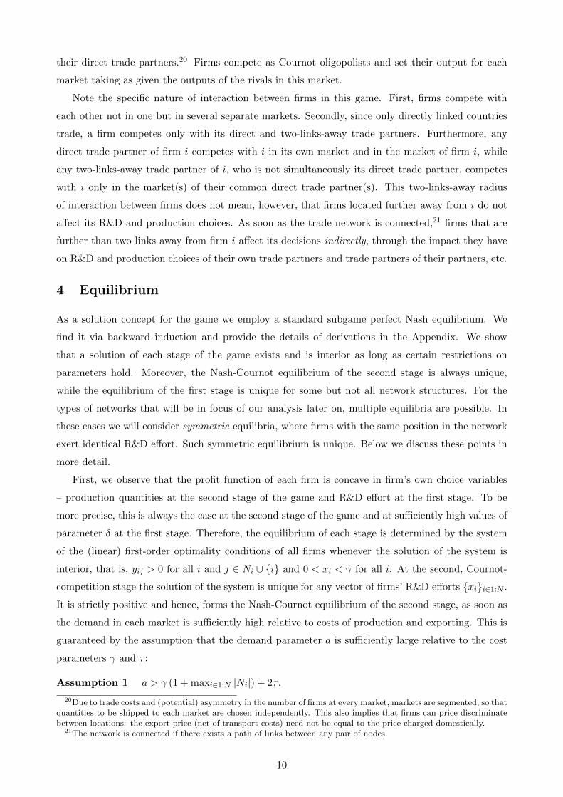
For simplicity, we focus on hub-and-spoke structures where all hub nodes are the same and all

spoke nodes are the same. This means that the network can be described by just four parameters:

nh, the number of direct trade partners of a hub; ns, the number of direct trade partners of a spoke;

ψ, the share of hubs among direct trade partners of a hub; and ϕ, the share of spokes among direct

trade partners of a spoke. Asymmetry of the network is captured by considering 1 ≤ ns < nh, and

the larger the difference between nh and ns, the larger the degree of asymmetry. The values of ψ and

ϕ, on the other hand, determine the composition of countries’ direct trade partners, that is, the exact

pattern of asymmetry in the network. We consider 0 ≤ ψ,ϕ < 1, where ϕ = ψ = 0 represents the

case in which hubs trade exclusively with spokes and vice versa.23 Clearly, not all combinations of

the four parameters are feasible but those that are feasible form a rich set of different hub-and-spoke

architectures.24 Some examples are presented in Table 1, where Types 1 - 5 of the hub-and-spoke

network differ either in their degree of network asymmetry (the difference between nh and ns) or in

the pattern of asymmetry (the values of ψ and ϕ).

In trade policy, hub-and-spoke networks can be viewed as a representation of regional/preferential

type of trade. When signed by members of the WTO, regional trade agreements signify a major

departure from the basic WTO principle of non-discrimination, according to which all WTO countries

are obliged to grant each other unconditionally any benefit or privilege affecting custom duties and

23The examples of ϕ = ψ = 0 are Type 1 and 3 networks in Table 1. We also note that setting ns = nh eliminates thedifference between hubs and spokes and turns the network into a symmetric network of degree ns = nh (ψ and ϕ aremeaningless in this case). Similarly, setting ϕ = ψ = 1 effectively splits the network into two symmetric components ofdegree ns and nh.

24Below we will show that the dependence of equilibrium R&D efforts of all firms on each of these four parametersis monotone. This then allows a comparison of R&D across many of the feasible hub-and-spoke structures.

12

Table 1: Examples of hub-and-spoke trade networks

Network characteristics Network

Type 1: Single star (nh bilaterals of a hub with spokes)

nh > 1, ns = 1, ψ = 0, ϕ = 0

Type 2: Stars with linked hubs

nh > 1, ns = 1, ψ > 0, ϕ = 0

Type 3: Stars sharing spokes

nh > 1, ns > 1, ψ = 0, ϕ = 0

Type 4: Stars with linked hubs, sharing spokes

nh > 1, ns > 1, ψ > 0, ϕ = 0

Type 5: Stars where some spokes are linked with each other

nh > 1, ns > 1, ψ = 0, ϕ > 0

Remark: Red nodes indicate hubs, green nodes indicate spokes.

charges on equal, non-discriminatory basis.25 In regional trade agreements (customs unions and free-

trade areas), countries within the agreement are treated more favorably than those outside: import

tariffs are completely eliminated between the members of the agreement, but kept on imports from

the rest of the world. Regional trade agreements have become prevalent in the last two decades, with

some countries being parties to several agreements.26 This results in the network where different

regional trade agreements “overlap”, forming the hub-and-spoke structure of the type considered

here.

In what follows, we focus on our key question of interest and study the effects of asymmetry in

the hub-and-spoke system on R&D decisions of firms. To this end, we first derive the equilibrium

levels of R&D in the hub-and-spoke system, focusing on the symmetric equilibrium, where all hubs

exert identical R&D effort x∗h and all spokes exert identical R&D effort x∗s. Those can be found from

the system of the first-order conditions (10), which in case of the hub-and-spoke network reduces to

two equations. The equations and their unique closed-form solution are provided in the Appendix.27

With this solution in hand, we then do comparative statics and examine the impact on R&D of

25See section 5.2 for further description of the main WTO principles.26See Figure 4 and examples of regional trade agreements in footnote 11.27See the proof of Proposition 1 in Appendix A.

13

a change in each of the four parameters describing the hub-and-spoke network. First, we examine

the effects of a change in ns, nh or both, which allows evaluating the effects of asymmetry in the

trade network. Then we study the implications of a change in ψ or φ, which for a given degree of

asymmetry describe how the composition of countries’ trade partners matters for firms’ incentives to

innovate.

Our main findings from this comparative statics analysis can be summarized as follows. First,

the larger the degree of asymmetry associated with an increase in nh or a decrease in ns or both,

the larger the equilibrium R&D of a hub. On the contrary, for a spoke the larger the degree of

asymmetry, the lower the equilibrium R&D, at least when certain conditions hold. As a result, a

larger asymmetry in the trade network leads to a larger disparity in innovation efforts of hubs and

spokes. Moreover, for a given degree of asymmetry, R&D of both a hub and a spoke increases in the

share of spokes among their direct trade partners. Formally, these findings are stated below, and

they are illustrated with Figures 5 and 6 in the Appendix.28

Proposition 1 (hub-and-spoke network). Consider hub-and-spoke trade networks, where ns <

nh ≤ n for some n > 1. Suppose that demand in each country is sufficiently large (Assumption 1)

and R&D is sufficiently costly (Assumption 2) for all ns < nh ≤ n. Then there exists ∆ > 0 such

that for any δ ≥ ∆ and for any ns < nh < n and 0 ≤ ψ,ϕ < 1, the following statements are fulfilled:

1. the equilibrium R&D effort x∗h of a hub is monotonically increasing in the number of hub’s

direct trade partners, nh, and monotonically decreasing in the number of spoke’s direct trade

partners, ns;

2. the equilibrium R&D effort x∗s of a spoke is monotonically decreasing in the number of hub’s

direct trade partners, nh;

3. the equilibrium R&D effort x∗s of a spoke is monotonically increasing in the number of spoke’s

direct trade partners, ns, if at least one of the conditions holds:

(a) the trade costs are sufficiently high: τ ≥ 1−ϕ3−2ϕ(a− γ),

(b) the share of other spokes among direct trade partners is at least 1/3: ϕ ≥ 13 ,

(c) the gap between nh and ns is relatively small: nh ≤ n2s, that is, 1 < nh

ns≤ ns.

4. Equilibrium R&D efforts of both a hub and a spoke are monotonically increasing in the share

of spokes among their direct trade partners: x∗h is monotonically decreasing in ψ, and x∗s is

monotonically increasing in ϕ.

Parts 1. and 3. of the proposition state that the larger the number of directly accessible markets

of a firm, the higher the incentives to innovate, – always for a hub and under conditions (a) – (c)

for a spoke. Further, parts 1., 2. and 4. of the proposition imply that for a given number of

28Both figures are produced using the following parameter values: γ = 7, b = 1, n = 10, τ = 2; a and δ fulfillAssumptions 1 and 2. In addition, for Figure 5, we set ψ = ϕ = 0 and for Figure 6, nh = 6, ns = 2.

14

direct trade partners, the larger the number of competitors in these markets, the lower the incentives

for innovation. In fact, the latter suggests that the “pure” competition effect of trade on R&D,

considered when only the number of firm’s competitors increases but the size of the market remains

unchanged, is negative: two-links-away trade partners dampen R&D of a firm.29 Still, the impact of

direct trade partners on R&D tends to be positive. That is, the positive scale effect of trade between

any directly linked countries is strong enough to outweigh the negative competition effect. This is

always true for hubs, and in a range of specified cases (a) – (c) for spokes.30

To grasp the intuition for the role of asymmetry described in Proposition 1, recall that in this

model the key determinant of firms’ incentives to innovate is the size of its overall market. For a

hub, a larger asymmetry is associated with a larger number of directly accessible markets (higher

nh) and lower number of competitors at least in some of these markets (lower ns). For a spoke,

the implications of asymmetry are the opposite. Moreover, for any given nh and ns, the larger

the share of spokes among direct trade partners of a country (hub or spoke), the lower the foreign

competition. As a result, the aggregate demand of a firm in a hub is larger when asymmetry is

large, and particularly large if the share of spokes among its direct trade partners is high. For a

spoke, the aggregate demand tends to be lower in highly asymmetric networks, and particularly low

if the share of spokes among its direct trade partners is small. This variation in aggregate demand

is translated into a difference in R&D incentives, so that increasing asymmetry amplifies R&D of a

hub but reduces R&D of a spoke.

It remains to understand conditions (a) – (c) which ensure that an increase in ns promotes spokes’

R&D investments. Recall that the specification of a hub-and-spoke trade network in this model is

such that an increase in the number of a spoke’s direct trade partners ns is associated with an increase

in the number of both types of partners – hubs and spokes. Then since the market of a hub is “small”

– smaller than the market of a spoke, an increase in the spoke’s foreign market share due to an access

to new markets may actually be smaller than a decrease in its domestic market share due to increased

competition. As a result, a positive scale effect of an increase in ns on spoke’s market size and R&D

may be dominated by a negative competition effect.31 Conditions (a) – (c) ensure that this would

not be the case by restraining the competition effect of trade. Namely, an increase in ns is certain

to expand spoke’s market size and R&D if either (a) the trade costs of firms are sufficiently high to

restrict the amount of exports from new trade partners, or (b) hubs represent only a minor share

of direct trade partners of a spoke, or alternatively, (c) the number ns of competitors in a spoke’s

market is comparable to nh, so that the loss in the domestic market share of a spoke does not exceed

the gain in a new hub’s market.

29This also means that the negative market-share component of the competition effect outweighs its positive markupscomponent.

30In Supplementary Appendix (Appendix C) we further investigate the impact of direct and two-links-away tradepartners on R&D of a firm in a generic network under the assumption of small local effects. Consistent with the resultof Proposition 1 for hub-and-spoke networks, we find that in a generic network, new direct trade partners (mostly)increase R&D of a firm, and this effect is stronger, the smaller the number of competitors in the new markets.

31This outcome seems to be rather rare though. For example, by calculating the model for the star network undervarious parameter assumptions, we find that initiating trade with the hub decreases R&D of a spoke only when thenumber of competitors in the hub’s market (other spokes) is above 100.

15

The comparative statics results of Proposition 1 can be employed to rank R&D efforts of firms in

different types of hub-and-spoke networks. For example, with respect to hub-and-spoke networks of

Table 1, Corollary 1 describes the comparisons that can be made. It uses the notation x∗hi for R&D

of a hub and x∗si for R&D of spoke in Type i of the hub-and-spoke structure, where i ∈ 1 : 5.

Corollary 1. Consider Types 1–5 of the hub-and-spoke trade network. Suppose that (i) nh is the

same across all types, (ii) ns is the same across all types where ns > 1 (Types 3, 4 and 5), and (iii)

ψ is the same across all types where ψ > 0 (Types 2 and 4). Then firms’ equilibrium R&D efforts in

Types 1–5 of the hub-and-spoke structure can be ranked as follows:

x∗h1 > x∗h3 > x∗h4, x∗h1 > x∗h2 > x∗h4, and x∗s5 > x∗s3 > x∗s1, x∗s4 > x∗s2.

The intuition for these comparisons is simple. As before, a ranking of firms’ R&D efforts is a

result of an analogous ranking of firms’ aggregate market sizes. Note that amongst all hub-and-

spoke networks, a star (Type 1 network) is the one where the hub enjoys the lowest competition

in its foreign markets. Therefore, for a fixed number of a hub’s direct trade partners, the hub of a

star has the largest aggregate market size. As the number of rival firms in a hub’s foreign markets

increases, the aggregate market size of the hub declines. This is the case when either the number of a

spoke’s direct trade partners, ns, increases (Type 3 network), or the share of hubs among direct trade

partners, ψ, grows (Type 2 network), or both changes in ns and ψ happen simultaneously (Type 4

network). Furthermore, the larger the increase in ns and ψ, the smaller the size of a hub’s aggregate

market.

For spokes, the situation is reversed. In the star (Type 1 network) each spoke has an access

to a single foreign market. Therefore, given a fixed number of a hub’s direct trade partners, a

spoke’s market in the star is smaller than in other hub-and-spoke trade networks. As the number of

direct trade partners of a spoke, ns, increases (Type 3 network), the market of a spoke expands. It

expands even further if the share of spokes among direct trade partners, ϕ , grows (Type 5 network).

Moreover, the larger the increase in ns and ϕ, the larger the aggregate market size of a spoke.

To further examine the effects of asymmetry in the trade network, in the next section we compare

our results for a hub-and-spoke network with those for a symmetric network, where all countries have

the same number of direct trade partners. This will also allow us to demonstrate that in any hub-and-

spoke trade network R&D of a hub is strictly larger than R&D of a spoke, as the former is larger and

the latter is smaller than R&D of a firm in the symmetric network. Intuitively, a symmetric network

can be regarded as a “special case” of a hub-and-spoke structure, where ns = nh, and all firms

exert the same R&D effort. Then as the asymmetry is “introduced” into such a network through an

increase in nh or a decrease in ns, hubs do more and spokes do less R&D than a representative firm

in the symmetric system.

This, together with the results of Proposition 1 emphasizes the importance of taking into account

the asymmetry of the trade network in determining R&D decisions of firms. Moreover, interpreting

our findings in application to regional/preferential trade, we conclude that allowing for regional trade

16

agreements in the WTO leads to a situation where firms in hub economies do more R&D than firms

in spoke countries, and the more asymmetric the trade relations become, the larger the gap between

R&D investments. In addition, the expansion of the regional trade network through a conclusion of

new agreements (creation of new links or new links and nodes) augments R&D of some but reduces

R&D of some other countries. The effect of a new trade agreement on R&D tends to be positive for

the immediately involved countries but negative for their existing trade partners.

5.2 Symmetric trade networks. Comparison with asymmetric networks

To better understand the effects of asymmetry, let us now consider a class of symmetric networks and

then compare R&D of firms in this setting with R&D of hubs and spokes in asymmetric networks. In

contrast to hub-and-spoke structures, in symmetric, or regular trade networks, each country has the

same number n of direct trade partners. n is sometimes called the degree of a symmetric network.

When n = 1, the network consists of one or more simple bilateral agreements, and when n = N − 1,

the network is complete, so that every country has an agreement with every other country.

Figure 1: Complete network with 8 countries

The case of a complete network can be thought of as representing multilateral trade between

countries. In general, multilateral trade is characterized by two fundamental principles of the GATT:

“reciprocity” and the “most favoured nation” principle of non-discrimination. The reciprocity prin-

ciple implies that each country agrees to reduce its trade barriers in return for a reciprocal reduction

by another; the non-discrimination principle states that all countries in the multilateral trade system

should be treated equally, that is, tariffs imposed by a country on imports from any other country

in the system must be the same. In our model, when all countries are linked with each other and

tariffs on all trade links are the same, – for example, zero, as in case of free trade agreements, – the

non-discrimination principle applies. And the reciprocity principle is obviously fulfilled, too, in its

extreme form since tariffs are reduced to the same level not only in trade within each pair of countries

but also across pairs.

In the symmetric network, all countries are identical, and each firm exerts the same R&D effort

in the symmetric equilibrium. It can be found from a single first-order condition (cf. (10)):[−(n+ 1)3

(n+ 2)2+ δb

]x+ 2n

n+ 1

(n+ 2)2x+ n

(n+ 1)(n− 1)

(n+ 2)2x =

(n+ 1)2

(n+ 2)2(a− γ) +

n+ 1

(n+ 2)2(−2τn+ τn),

17

which leads to:

x∗(n) =a− γ − n

n+1τ

−1 + δb(1 + 1

n+1

)2 . (5)

We study the functional dependence of this equilibrium R&D effort on n, and obtain that the larger

the number of a country’s direct trade partners, the stronger the incentives of a firm to invest in

R&D. Moreover, this turns out to be the case even despite the fact that the equilibrium profit of

a firm declines as the number of direct trade partners increases. Both of these comparative statics

results are stated in Proposition 2, and Figure 7 provides an illustration:32

Proposition 2 (symmetric network). Consider symmetric networks of degree n, where n < n

for some n ≥ 1. Suppose that demand in each country is sufficiently large (Assumption 1) and

R&D is sufficiently costly (Assumption 2) for all n < n. Then firm’s equilibrium R&D effort x∗ is

monotonically increasing in n, while firm’s profit π is monotonically decreasing in n for any n < n.

Intuitively, as the symmetric network of trade agreements expands – due to an access of a new

country or a formation of new agreements between the existing countries, – the reduction in the

domestic and foreign market shares suffered by each firm is exactly compensated by the participation

in the new market. That is, the negative market share effect associated with an increased competition

exactly offsets the positive scale effect associated with an access to a new market. As a result, opening

to trade with a new country affects R&D of each firm only through the remaining component of the

competition effect – the reduction in price markups. Then since this markups reduction increases

firm’s aggregate demand, it also increases R&D, so that in equilibrium, R&D of each firm is increasing

in the number of its direct trade partners.33 On the other hand, the profit of each firm declines as a

result of increasing R&D expenditures and decreasing prices.34

One interpretation of Proposition 2, when applied to the case of a complete network, is that the

expansion of the multilateral trade system promotes R&D in every country. It also suggests that the

R&D investment of a firm in the multilateral agreement with n ≥ 2 is higher than R&D of a firm in

the bilateral agreement (n = 1), which in turn is higher than R&D in autarky (n = 0). Furthermore,

as a consequence of the above, also the aggregate level of R&D in the multilateral trade system

increases in the size of the system and exceeds the aggregate R&D of the same number of countries

that are either involved in simple bilateral agreements or do not trade with each other at all.

Now, bringing the results of our equilibrium analysis in this and the preceding section together,

we can compare R&D incentives of firms in symmetric and hub-and-spoke trade networks. Under

the same demand and cost parameter restrictions as employed in our analysis above, the following

32The equilibrium profit of a firm in the symmetric network is given by equation (12) in the Appendix. Figure 7 isproduced using the same parameter values as for Figures 5 and 6: γ = 7, b = 1, n = 10, and τ = 2; a and δ fulfillAssumptions 1 and 2.

33Note that in contrast to this case of a symmetric network, in the asymmetric, hub-and-spoke structure, the in-teraction of scale and competition effects of trade is not so straightforward, and the negative, market-share effect ofcompetition is generally not offset by the positive scale effect.

34Figure 7 also demonstrates that the rates of increase in R&D and decrease in profit are both declining in n.This is implied by the fact that the markup-reducing effect of trade in the symmetric network becomes weaker as thenetwork expands. In fact, it is easy to show that the price in each market is a decreasing and convex function of n, asdemonstrated by Figure 8 in the Appendix.

18

proposition states an important result. It claims that in any hub-and-spoke network, R&D of a hub

is larger than R&D of a spoke. Moreover, given the same number nh of direct trade partners, R&D

of a hub, x∗h, is larger than R&D of a firm in the symmetric network, x∗(nh), while for spokes, the

opposite is true: given the same number ns of direct trade partners, R&D of a spoke, x∗s, is smaller

than R&D of a firm in the symmetric network, x∗(ns).

Proposition 3 (comparison of symmetric and hub-and-spoke networks). Consider a hub-

and-spoke network defined by parameters 0 ≤ ψ,ϕ < 1 and 1 ≤ ns < nh ≤ n for some n > 1, and any

symmetric trade networks of degree ns and nh. Suppose that demand in each country is sufficiently

large (Assumption 1) and R&D is sufficiently costly (Assumption 2) for all ns < nh ≤ n. Then there

exists ∆ > 0 such that for any δ ≥ ∆, R&D of firms in hub-and-spoke and symmetric networks can

be ranked as follows:

x∗h > x∗(nh) > x∗(ns) > x∗s.

The proof of this proposition is based on the idea that a symmetric network of degree nh can be

regarded as a hub-and-spoke network “composed only of hubs”, that is, where ns in the hub-and-

spoke network has increased to become equal to nh. Similarly, a symmetric network of degree ns

can be regarded as a hub-and-spoke network “composed only of spokes”, where nh has decreased to

become equal to ns.35 Then inequalities x∗h > x∗(nh) and x∗(ns) > x∗s follow immediately from parts

1 and 2 of Proposition 1 stating that R&D of a hub, x∗h, is decreasing in ns and R&D of a spoke, x∗s,

is decreasing in nh. The last, “connecting” inequality x∗(nh) > x∗(ns) is implied by Proposition 2,

according to which R&D of a firm in the symmetric network is increasing in its degree.

As before, an intuitive explanation for the obtained comparison of firms’ R&D levels has to do

with the comparison of their market sizes. Indeed, for any number of direct trade partners, the

aggregate market size of a hub in a hub-and-spoke network is larger than that of a firm in the

symmetric network, and the opposite is true for a spoke. A simple calculus provides the key insight.

While in a symmetric network of degree nh, the number of firm’s competitors is nh in each of its

foreign markets, in a hub-and-spoke network, the number of hub’s competitors is nh only in ψnh of

its foreign markets, while in the other markets it is less than nh. Symmetrically, for a spoke, the

number of its competitors in the foreign markets is larger than for a firm in a symmetric network of

degree ns. Therefore, for the same number of direct trade partners, benefits of innovation for a hub

are higher and for a spoke lower than for a country in the symmetric network.

Our next proposition combines the results of Proposition 3 and Corollary 1 and provides the

ranking of equilibrium R&D efforts of firms in different types of hub-and-spoke networks (see Table

1) and in the symmetric networks.

Proposition 4 (extended comparison). Consider Types 1–5 of the hub-and-spoke trade network.

Suppose that (i) nh is the same across all types, (ii) ns is the same across all types where ns > 1

35When ns = nh, ψ and ϕ become meaningless and drop from the analysis of hub-and-spoke networks. Furthermore,in the proof we note that such transformation from a hub-and-spoke to symmetric network may require adding ordeleting some nodes, but as R&D decisions of firms are fully determined by parameters ns, nh, ψ and ϕ and not bythe overall network size, the total number of nodes in the network is irrelevant.

19

(Types 3, 4 and 5), and (iii) ψ is the same across all types where ψ > 0 (Types 2 and 4). Then firms’

equilibrium R&D efforts in Types 1–5 of the hub-and-spoke network and in the symmetric network

can be ranked as follows:36

x∗h1 > x∗h3 > x∗h4 > x∗(nh) > x∗(ns) > x∗s5 > x∗s3 > x∗s1

and

x∗h1 > x∗h2 > x∗h4 > x∗(nh) > x∗(ns) > x∗s4 > x∗s2.

The first sequence of inequalities is demonstrated with Figure 2 below. Figure 9 in the Appendix

provides an analogous illustration for the second sequence.

Thus, R&D investments of firms differ substantially across symmetric and asymmetric trade

networks and across hub and spoke countries within an asymmetric network. The highest R&D

incentives exist for a hub, especially for a hub in the star (Type 1 network), whereas for a spoke in

the star R&D incentives are the lowest. As the number of direct trade partners of a spoke and/or the

share of spokes (hubs) among direct trade partners of each spoke (hub) increase, the levels of R&D

investment of hubs and spokes draw closer together. They coincide at the level of R&D investment

of a firm in the symmetric network, which therefore, takes an average position – lower than R&D of

a hub but higher than R&D of a spoke.

Finally, in addition to the comparison of firms’ individual R&D investments, we compare the

aggregate R&D of the same total number of countries in the complete trade network and in the

simple star. While the latter network can be thought of as representing a multilateral trade system,

the former is a trade arrangement where one country, the hub, has several bilateral agreements with

spoke countries. We find that even though R&D of the hub in a star is higher than R&D of a single

country in the multilateral system, the aggregate R&D in the star is lower than in the multilateral

agreement. This observation is demonstrated with Figure 10 in the Appendix.

5.3 Welfare analysis

To complement the analysis of the effects of asymmetry in the trade network on firms’ R&D, this

section compares the welfare implications of trade within a symmetric network and within a star,

the simplest type of the hub-and-spoke structure. A higher degree of asymmetry in the star network

is associated with a larger number of spokes, that is, hub’s direct trade partners, while the number

of spokes’ direct trade partners is fixed at one. In what follows, the social welfare of country i, Wi,

is defined as the sum of firm i’s profit, πi, and consumer surplus, CSi, where

CSi =1

2b(a− pi)2 (6)

due to linearity of the demand function in (1).

We find that in both types of trade network, symmetric and a star, the level of welfare and the

impact on welfare of a new trade agreement depends on the value of trade costs τ and, in a certain

36The last inequality in both sequences requires, in addition, that at least one of three conditions (a) – (c) ofProposition 1 holds, under which x∗s is increasing in ns.

20

Figure 2: Equilibrium R&D efforts in the symmetric and hub-and-spoke trade networks as a functionof nh (upper panel) and as a function of ns (lower panel).

21

range of trade costs, on the number of country’s existing trade partners. Starting from the case of

an asymmetric, star network, our first proposition states that when the trade costs are relatively low

(below a certain threshold τ), the welfare of the hub economy increases in the number of its direct

trade partners, n, while the welfare of spokes declines. That is, a higher degree of asymmetry in the

star network widens the welfare gap between the hub and the spokes. On the other hand, at high

trade costs (above another, larger threshold τ), the welfare of both, the hub and the spokes, decreases

in the number of hub’s trade partners, and at medium trade costs (between the two thresholds), the

impact of a new trade partner depends on the number of hub’s existing trade partners.

Proposition 5 (welfare in a star). Consider a star network, where the number of hub’s di-

rect trade partners nh < n for some n ≥ 1. Suppose that demand in each country is sufficiently

large (Assumption 1) and R&D is sufficiently costly (Assumption 2) for all nh < n. Then for

any nh < n, there exists ∆ > 0 such that for any δ ≥ ∆, the social welfare of a spoke economy

is monotonically decreasing in nh (at all τ ≥ 0). Furthermore, as soon as an additional restric-

tion a > γ(

1 +nh(2n3

h+12n2h+51nh+16)

9(nh+2)

)holds, there exist ∆ > 0 and two thresholds of trade costs

0 < τ ≤ τ , such that for any δ ≥ ∆, the following statements are fulfilled:

1. the social welfare of the hub economy is monotonically increasing in nh for any τ < τ and it is

monotonically decreasing in nh for any τ > τ ;

2. for τ ∈ [τ , τ ], there exists n(τ), 1 ≤ n(τ) ≤ n, such that the social welfare of the hub is

monotonically increasing in nh for any nh ≤ n(τ) and it is monotonically decreasing in nh for

nh > n(τ).

Such a dependence of social welfare of the hub on trade costs τ and, at medium values of τ ,

on the status quo number of hub’s trade partners can be explained as follows. At low trade costs

(below τ), an access to a new, spoke market is cheap and leads to a large expansion of the overall

production at the hub firm. Then even though the price in the hub’s own market declines due to an

increased competition, the profit of the hub firm increases. Moreover, a lower price in the hub market

benefits the consumers. As a result, at low trade costs, the welfare of the hub improves due to an

increase in both, firm’s profit and consumer surplus. As trade costs grow, exploitation of the spoke

markets by the hub becomes more expensive, and a larger number of trade partners is associated

with lower profits for the hub firm. In fact, when trade costs are high enough, the profit reduction

associated with an extra trade partner is larger than the value of a simultaneous increase in the

consumer surplus, so that the welfare of the hub declines. At first, this negative impact of a new

trade partner shows only in large star networks, as the rate of increase in consumer surplus in such

networks is particularly low (see Figure 12). However, when trade costs become very high (above τ),

benefits from trade for the hub are minor in star networks of any size, and a new trade agreement

unequivocally reduces hub’s welfare. By contrast, in a spoke economy, welfare is decreasing in nh at

all levels of trade costs. While almost invariable price in a spoke market keeps the consumer surplus

22

constant, the profit of a spoke firm at larger nh is smaller as a result of a lower price and reduced

market share in the hub, spoke’s only trade partner.

In a symmetric trade network, the welfare changes associated with a larger number of direct

trade partners are similar to those at the hub in a star. At low trade costs, the social welfare of each

country is increasing in the number of its direct trade partners, n, and it is decreasing in n at high

trade costs. At medium trade costs, the impact of a new trade agreement on welfare depends on the

number of country’s existing trade partners: at low levels of country’s overall trade exposure, the

impact of a new trade agreement on the welfare is positive but it turns negative as the number of

country’s trade partners exceeds a certain threshold.

However, differently from the case of a star network, in a symmetric trade network, trade with a

new partner at low and medium trade costs improves country’s welfare due to an increase in consumer

surplus only, as firm’s profits decline even when trade costs are low. The latter is explained by the

fact that a new trade agreement in a symmetric network leads to a much smaller expansion of a firm’s

aggregate market as compared to the boost in aggregate demand of the hub in a star. Therefore,

firm’s overall production in the symmetric network increases only a little when its number of accessible

markets grows, while the price at each market is slashed by tighter competition.37 Then, as the level

of trade costs increases, the decline in profits associated with new foreign markets becomes even

stronger and at some point, it outweighs the increase in consumer surplus. Just as in a star network,

first, this negative impact of a new trade partner on welfare shows only in trade networks with a large

number of existing trade partners, where the rate of increase in consumer surplus is particularly low

(see Figure 12). But at sufficiently high trade costs, a new trade agreement reduces social welfare of

a country irrespective of its current degree of trade exposure. Formally, the welfare implications of

trade in a symmetric network are stated by Proposition 6:

Proposition 6 (welfare in a symmetric network). Consider a symmetric network of degree n,

where n < n for some n ≥ 1. Suppose that demand in each country is sufficiently large (Assumption

1) and R&D is sufficiently costly (Assumption 2) for all n < n. Then for any n < n, the consumer

surplus of a country in a symmetric trade network of degree n is monotonically increasing in n.

Furthermore, as soon as an additional restriction a > γ(1 + n+ 2n/(n+ 2)) holds, there exist ∆ > 0

and two thresholds of trade costs 0 < τ ≤ τ , such that for any δ ≥ ∆, the following statements are

fulfilled:

1. the social welfare of a country is monotonically increasing in n for any τ < τ and it is mono-

tonically decreasing in n for any τ > τ ;

2. for τ ∈ [τ , τ ], there exists n(τ), 1 ≤ n(τ) ≤ n, such that the social welfare of a country is

monotonically increasing in n for any n ≤ n(τ) and it is monotonically decreasing in n for

n > n(τ).

37Formally the negative impact of an increase in n on firm’s profit has been established by Proposition 2.

23

Proposition 6 is illustrated with Figure 3. Other figures showing the dependence on n of countries’

profits, consumer surplus and welfare in both symmetric and star networks are presented in the

Appendix (Figures 12 – 14). Notice that the level of unit trade costs at which the social welfare of

a country in a symmetric network or of the hub in a star decreases in n is “very high” relative to

other costs and prices in each market. This implies that at low and medium trade costs, – such as in

case of zero tariffs in free trade agreements and custom unions, – the expansion of a symmetric trade

network improves the welfare of every country, and similarly, the expansion of the star increases the

welfare of the hub.

Figure 3: Social welfare of a country in a symmetric trade network of degree n.

Furthermore, the results of our numerical analysis imply that for any number nh of direct trade

partners and any trade costs, the social welfare of the hub in a star is higher than the welfare of a

country in a symmetric network (Figure 14). On the other hand, the welfare of a spoke in the star

is lower than the welfare of both the hub and a country in the symmetric network at least when

trade costs are not too high.38 The difference between the welfare of the hub and a country in the

symmetric network is driven by a large disparity in firms’ profits: while the consumer surplus of the

hub and of a country in the symmetric network are essentially the same, the profit of the hub firm is

much higher than the profit of a firm in the symmetric network. For a spoke in the star, the lowest

level of welfare is mainly due to the lowest consumer surplus. At the aggregate level, the results

point at the benefits of trade in the symmetric network: for the same total number of countries, the

aggregate welfare in the symmetric, complete network exceeds the welfare in the star, with a larger

difference obtained at low trade costs (Figure 15).

38These findings find support in earlier studies. For example, Baldwin (2004), Kowalczyk and Wonnacott (1992),Deltas et al. (2006), Lloyd and Maclaren (2004), and De Benedictis et al. (2005) find that the welfare and incomelevels of spokes are lower than those of hubs and of countries in the complete network.

24

For trade policy, the findings derived in this section imply that asymmetry in trade relations

between countries benefits the hub but harms the spoke economies. In particular, in the regional

trade system where one (hub) economy has several bilaterals with other countries (spokes), the welfare

of the hub is larger than the welfare of a spoke, and the expansion of such trade system increases this

welfare gap, at least as long as the trade costs are not too high. On the other hand, the expansion

of the multilateral trade system (the complete network) improves the welfare of every country and

also offers higher aggregate welfare than a regional, star system, even though each country’s welfare

is lower than that of the hub in the star.

Lastly, notice that if we interpret trade costs as tariffs, then the social welfare of country i can

be defined alternatively as

Wi = πi + CSi + Ti,

where Ti = τ∑

k∈Niyki is the total trade tariffs collected by country i. Given such definition of

welfare, we find numerically that the social welfare of each country within a symmetric trade network

and of the hub in a star is monotonically increasing in the number of their direct trade partners, nh,

for any value of trade costs. The social welfare of a spoke country is decreasing in nh, just as in case

of the original welfare formulation. These findings are illustrated with Figure 16.

6 Conclusions and policy implications

This paper develops a model of intra-industry trade with firm-level productivity improvements via

R&D. Trade relations between countries are represented by a network, and the two large classes of

networks considered are hub-and-spoke and symmetric networks. In this framework we study the

effects of asymmetry in the number of countries’ trade partners on firms’ innovation incentives and

countries’ welfare.

We find that the trade network asymmetry does play an important role. First, with respect to

innovation, R&D investment of a hub is always larger than R&D of a spoke, and R&D of a firm

in the symmetric network is lower than in a hub but higher than in a spoke even if the number of

trade partners of a hub (resp., spoke) is the same as the number of trade partners of a country in the

symmetric network. Furthermore, the larger the degree of asymmetry, associated with an increase

in the number of direct trade partners of a hub or a decrease in the number of direct trade partners

of a spoke (or both), the larger the disparity in innovation efforts of hubs and spokes.

Intuitively the role of asymmetry in a trade network for R&D decisions of firms can be understood

in light of its effects on firms’ aggregate demand. Indeed, the aggregate demand of a firm determines

its incentives to innovate, as larger demand amplifies the returns but does not affect the cost of R&D.

Thus, any change in the degree of trade network asymmetry that increases firm’s aggregate demand,

also increases its R&D incentives, and vice versa. For a hub, a larger degree of asymmetry in the hub-

and-spoke networks is associated with larger aggregate demand, as the number of directly accessible

markets is larger and/or the number of competitors at least in some of these markets is lower. On the

contrary, for a spoke, a larger degree of asymmetry implies smaller aggregate demand. A symmetric

25

network, on the other hand, can be regarded as a “special case” of a hub-and-spoke structure, where

the number of direct trade partners of a hub and a spoke are the same. The aggregate demand

of a firm in such network is in-between those of a hub and a spoke, where the latter obtain when

asymmetry is “introduced” through an increase or decrease in the number of direct trade partners of

some countries. This difference in the aggregate demand of hubs, spokes and firms in the symmetric

network translates into a difference in their R&D incentives. As a result, the largest R&D incentives

exist for a hub in the hub-and-spoke network, while for a spoke, the R&D incentives are the lowest.

For a firm in the symmetric network, R&D is lower than in a hub but higher than in a spoke.

Furthermore, concerning the welfare implications of trade in the symmetric network and in the

simple star network, we find numerically that for the same number of trade partners, the welfare of

the hub in a star is larger than the welfare of a country in the symmetric network, while the welfare

of a spoke in the star is the lowest. We also find that when the trade costs are not too high, an

increasing degree of asymmetry in the star network (due to an expansion in the number of hub’s

foreign markets) enhances the welfare of the hub but lowers the welfare of spokes. By contrast, in

the symmetric network, a larger number of countries’ trade partners improves the welfare of every

country.

The findings of the paper suggest some policy implications. First, interpreting the hub-and-spoke

network as a trade network that emerges in the process of regional/preferential trade liberalization,

and the symmetric complete network as a result of multilateral trade liberalization, we conclude that

R&D and welfare gains of regionalism versus those of multilateralism depend heavily on the relative

number of regional trade agreements signed by countries. If a country signs a relatively large number

of regional trade agreements and thus becomes a hub in the trade network, then its R&D/productivity

and social welfare are higher than R&D/productivity and welfare of a country in the multilateral

trade system. On the other hand, a country that is involved in a relatively small number of regional

trade agreements derives lower R&D and welfare gains than a country in the multilateral system.

This implies that from the perspective of a small economy, which can only become a spoke in the

regional trade system, the prospects for productivity improvements and welfare gains are generally

better in the multilateral trade system than in the regional system. In contrast, for hubs the regional

alternative is more attractive, and thus, allowing regional trade agreements in the WTO may inhibit

the pursuit of multilateral free trade by “powerful” hub economies. Furthermore, the finding that

opening to trade with new countries in the symmetric trade network promotes R&D and welfare

of every country (at least as long as trade costs are low) implies that an expansion of the WTO or

unification of several plurilateral blocks benefit all member states. Differently, in asymmetric regional

trade systems an expansion of the system tends to increase R&D and welfare of the countries that

are immediately involved in a new trade agreement but suppresses R&D and welfare of their existing

trade partners.

At last, considering the results of the paper in application to the inter-regional trade within one

country, we obtain that regions where businesses are better connected to markets in other parts of the

26

country outperform their more isolated neighbours, both in terms of welfare and firm productivity.

This points towards the importance of regional trade and business integration and provides new

insights into the reasons for large productivity and wealth gaps between regions in many countries.

A number of extensions remain for further research. First, note that in the current setting all

countries are regarded as absolutely identical in all but their position in the trade network. This allows

isolating the effects of trade network asymmetry and countries’ involvement in trade. Endogenizing

the trade network in such setting is bound to produce symmetric or almost symmetric network

structures, as demonstrated by the network formation models of Goyal and Joshi (2006) and Mauleon

et al.(2010). It would, therefore, be interesting to consider endogenous trade network formation in a

model where countries are a priori different in their market size and/or firms’ marginal production

costs. Such approach is likely to generate trade network asymmetries observed in the real world,

where countries that are larger and/or more productive are more involved in the international trade.

Second, an important direction for further research is testing the results of the paper empirically.

To the best of our knowledge, the impact on R&D and productivity of asymmetries in the network

of international trade and the issue of potential variations in the impact on R&D and productivity

of different types of trade liberalization (multilateral versus regional) have not been addressed in

the empirical research. Our theoretical findings suggest the relevance of this research direction.

More generally, they emphasize the importance of taking into account the asymmetry and degree

of asymmetry in countries’ trade exposure in any empirical investigation of the impact of trade on

innovation, productivity and countries’ welfare.

References

[1] Acemoglu, D., and J. Linn. 2004. ”Market Size in Innovation: Theory and Evidence from thePharmaceutical Industry.” The Quatrly Journal of Economics, 119(3): 1049-1090.

[2] Aghion, P., Bloom N., Blundell R., Griffith R., and P. Howitt. 2005. ”Competition and Innovation:An Inverted-U relationship.” The Quatrly Journal of Economics, 120(2): 701-728.

[3] Aghion, P., and R., Griffith. 2008. ”Competition and Growth: Reconciling Theory and Evidence.”Zeuthen Lectures. MIT Press: Cambridge, US.

[4] Alvarez, R., and R. Lopez. 2005. ”Exporting and Performance: Evidence from Chilean Plants.”Canadian Journal of Economics, 38(4): 1384-1400.

[5] Arkolakis C., Ramondo, N., Rodriguez-Clare, A., and S. Yeaple. 2014. ”Innovation and Produc-tion in the Global Economy”, NBER WP 18792.

[6] Atkeson A. and A. Burstein. 2010. ”Innovation, Firm dynamics, and International Trade,” Journalof Political Economy

[7] Aw, B. Y., Chung S., and M. J. Roberts. 2000. ”Producivity and Turnover in the Export Market:Micro-Level Evidence from the Republic of Korea and Taiwan.” World Bank Economic Review,14(1): 65-90.

[8] Bagwell, K., and R. W. Staiger. 1997. ”An Economic Theory of GATT.” American EconomicReview , 89 (1), 215 248.

[9] Bagwell, K. and R. W. Staiger. 2002. ”The Economics of the World Trading System,” Cambridge:MIT Press.

27

[10] Baier, S. L., Bergstrand, J. H., Egger P., and P. A. McLaughin. 2008. ”Do Economic IntegrationAgreements Actually Work? Issues in Undertanding the Causes and Consequences of the Growthof Regionalism,” The World Economy. 31: 461497.

[11] Baldwin, R. E., 1995. ”A Domino Theory of Regionalism,” in Richard E. Baldwin, P. Haaparantaand J. Kiander, eds. Expending Membership in the European Union. Cambridge, UK: Cambridgeuniversity Press, 25-48.

[12] Baldwin, R. E. 2004. ”The Spoke Trap: Hub-and-Spoke Regionalism in East Asia.” CNAECResearch Series 04-02, Korean Institute for International Economic Policy.

[13] Baldwin, R. E. 2005. ”Stepping Stones or Building Blocks? Regional and Multilateral Integra-tion.” in Regional Economic Integration in a Global Framework, ed. J. McKay, M. O. Armengol,and G. Pineau. European Central Bank, Frankfurt.

[14] Bernard, A. B., Jensen J. B., and P.K. Schott. 2006. ”Falling Trade Costs, Heterogeneous Firms,and Industry Dynamics.” Journal of Monetary Economics, 53: 917-937.

[15] Bernard, A. B., Redding S. J., and P.K. Schott. 2007. ”Comparative Advantage and Heteroge-neous Firms.” Review of Economic Staudies, 74(1): 31-66.

[16] Bernard, A. B., Redding S. J., and P.K. Schott. 2010. ”Multiple-Product Firms and ProductSwitching”, American Economic Review, 100(1): 70-97.

[17] Bernard, A. B., Redding S. J., and P.K. Schott. 2011. ”Multi-Product Firms and Trade Liber-alization”, Quarterly Journal of Economics, 126(3): 1271-1318.

[18] Bhagwati, J. 1993. ”Regionalism and Multilateralism: an Overview,” in New Dimensions inRegional Integration, ed. Melo and Panagariya.

[19] Bhagwati, J. 2012. ”Doha Round: Failure of Talks Means World Lost Gains That a SuccessfulTreaty Would Have Brought,” in The Economic Times, June 1.

[20] Brander, J.A. 1981. ”Intra-industry trade in identical commodities”, Journal of InternationalEconomics, 11: 1-14.

[21] Brander, J.A. and P. Krugman. 1983. ”A reciprocal dumping model of international trade”,Journal of International Economics, 15: 313-321.

[22] Bustos, P. 2011. ”Multilateral Trade Liberalization, Exports and Technology Upgrading: Evi-dence on the Impact of MERCOSUR on Argentinian Firms.” American Economic Review.

[23] Chen, M.X. and S. Joshi. 2010. ”Third-country effects on the formation of free trade agreements,”Journal of International Economics, Elsevier, vol. 82(2): 238-248.

[24] Chong, S. J., and Hur, J. 2008. ”Small Hubs, Large Spokes and Overlapping Free Trade Agree-ments.” The World Economy. 31(12): 16251665.

[25] D’Aspremont, C., and A. Jacquemin. 1988. ”Cooperative and Noncooperative R&D in Duopolywith Spillovers.” American Economic Review, 78: 1133-1137.

[26] De la Torre, A., and M. R. Kelly. 1992. ”The Regional Trade Arrangements.” IMF OccasionalPaper, 93, IMF, Washington, DC.

[27] De Benedictis, L., De Santis R., and C. Vicarelli. 2005. ”Hub-and-Spoke or Else? Free TradeAgreements in the ’Enlarged’ European Union.” ENERPI and ISAE.

[28] De Loecker, L. 2007. ”Do Exports Generate Higher Productivity? Evidence from Slovenia”,Journal of International Economics, 73 (1): 69-98.

[29] Del Gatto, M., Mion G., and G. I. P. Ottaviano. 2006. ”Trade Integration, Firm Selection andthe Costs of Non-Europe.” CEPR Discussion Paper No. 5730.

[30] Deltas, G., Desmet K., and G. Facchini. 2006. ”Hub-and-Spoke Free Trade Areas.” CEPRDiscussion Paper No. 5960.

[31] Devereux, M., and B. Lapham. 1994. ”The Stability of Economic Integration and EndofenousGrowth.” The Quaterly Journal of Economics, 109: 299-305.

[32] Dewit, G., and D. Leahy. 2015. ”Strategic R&D Commitment and the Gains from Trade”,manuscript.

[33] Dhingra, S. 2013. ”Trading Away Wide Brands for Cheap Brands”, American Economic Review,103(6): 2554-84.

28

[34] Dixit, A. K. and G. M. Grossman. 1986. ”Targeted Export Promotion with Several OligopolisticIndustries.” Journal of International Economics, 21(3-4): 233-249.

[35] Eckel, C. and J. P. Neary. 2010. ”Multi-Product Firms and Flexible Manufacturing in the GlobalEconomy,” Review of Economic Studies, 77(1): 188-217.

[36] Ekholm, K. and K. H. Midelfart. 2005. ”Relative Wages and Trade-Induced Changes in Tech-nology,” European Economic Review, 49: 16371663.

[37] Ethier, W. J. 1998. Regionalism in a Multilateral World, Journal of Political Economy, 106:1214-1245.

[38] Fagiolo, G., Reyes, J. and Schiavo, S. 2009. ”World-Trade Web: Topological Properties, Dy-namics, and Evolution.” Physical Review E 79(3), 36115.

[39] Falvey, R., D. Greenaway, and Z. Yu. 2006. ”Extending the Melitz Model to Asymmetric Coun-tries,” University of Nottingham GEP Research Paper.

[40] Feenstra, R. 2004. ”Advanced International Trade: Theory and Evidence,” Princeton UniversityPress, Princeton.

[41] Feenstra, R. and H. Ma. 2008. ”Optimal Choice of Product Scope for Multiproduct Firmsunder Monopolistic Competition,” in Elhanan Helpman, Dalia Marin, and Thierry Verdier, eds.,The Organization of Firms in a Global Economy, Cambridge, Mass.: Harvard University Press,chapter 6, 173199.

[42] Fergusson I. F. 2008, 2011. ”World Trade Organization Negotiations: The Doha DevelopmentAgenda,” CRS Report for Congress.

[43] Fung, M. 2002. ”Technological Opportunity and Economies of Scale in Research Productivity:A Study on Three Global Industries,” Review of Industrial Organization, 21, 419436.

[44] Furusawa, T., and H. Konishi. 2007. ”Free Trade Networks.” Journal of International Economics,72: 310-335.

[45] Goyal, S., and J. Moraga. 2001. ”R&D Networks.” RAND Journal of Economics, 32(4): 686-707.

[46] Goyal, S., and S. Joshi. 2006. ”Bilateralism and Free Trade.” International Economic Review,47 (3): 749-778.

[47] Griliches, Z. 1957. ”Hybrid Corn: An Exploration in the Economics of Technological Change.”Econometrica, 25: 501-522.

[48] Grossman, G. and E. Helpman. 1991. ”Innovation and Growth in the Global Economy,” TheMIT Press.

[49] Gustavsson, P., Hansson, P., Lundberg, L. 1999. ”Technology, Resource Endowments and Inter-national Competitiveness,” European Economic Review, 43: 15011530.

[50] Haaland, J. I., and H. J. Kind. 2008. ”R&D Policies, Trade and Process Innovation,” Journalof International Economics, 74(1): 170-187.

[51] Helpman, E. 1981. ”International Trade in the Presence of Product Differentiation, Economiesof Scale, and Monopolistic Competition: A Chamberlin-Heckscher-Ohlin Approach.” Journal ofInternational Economics, 11(3): 305-340.

[52] Horaguchi, H. H. 2007. ”Economic Analysis of Free Trade Agreements: Spaghetti Bowl Effectand a Paradox of Hub and Spoke Network,” Journal of economic integration, 22(3): 664-683.

[53] Impullitti, G., and O. Licandro. 2013. ”Trade, Firm Selection, and Innovation: The CompetitionChannel,” Discussion Papers 13/04, University of Nottingham, School of Economics.

[54] Jensen, R., and M. Thursby. 1986. ”A Strategic Approach to the Product Life Cycle”, Journalof International Economics, 21: 269-284.

[55] Jensen, R., and M. Thursby. 1987. ”A Decision Theoretic Model of Innovation, TechnologyTransfer, and Trade”, The Review of Economic Studies, 54(4): 631-647.

[56] Kali, R., and J. Reyes. 2007. ”The Architecture of Globalization: A Network Approach toInternational Economic Integration”, Journal of International Business Studies, 38: 595620.

[57] Kowalczyk, C., and R. Wonnacott. 1991. ”Substitute and Complement Trading Clubs.” Dart-mouth College, Department of Economics, working paper 91-16.

29

[58] Kowalczyk, C., and R. Wonnacott. 1992. ”Hubs and Spokes, and Free Trade in the Americas,”NBER Working Paper 4198.

[59] Kremer, M.. 2002. ”Pharmaceuticals and the Developing World,” Journal of Economic Perspec-tives, 26: 67-90.

[60] Krisha, K. and A. O. Krueger. 1995. ”Implementing Free Trade Areas: Rules of Origin andHidden Protection,” in James Levinsohn, Alan Deardorff and Robert Stern, eds. New Directionsin Trade Theory. Ann Arbor: University of Michigan Press.

[61] Krishna, P. 1998. ”Regionalism and Multilateralism: A Political Economy Approach,” QuarterlyJournal of Economics, 108, 1998, 227-251.

[62] Krishna, P. 2002. ”Are Regional Trading Partners Natural,” Journal of Political Economy.

[63] Krishna, P. 2004. ”The Economics of Preferential Trade Agreements,” in Handbook of Interna-tional Trade: Economic and Legal Analyses of Trade Policy and Institutions, Volume II (eds E. K.Choi and J. C. Hartigan), Blackwell Publishing Ltd, Oxford, UK. doi: 10.1002/9780470757697.ch9

[64] Krugman, P. R. 1979. ”Increasing Returns, Monopolistic Competition, and International Trade,”Journal of International Economics, 9 (4): 469-479.

[65] Krugman, P. R. 1980. ”Scale Economies, Product Differentiation, and the Pattern of Trade,”American Economic Review, 70 (5): 950-959.

[66] Licandro, O., and A. Navas-Ruiz. 2011. ”Trade Liberalization, Competition, and Growth.” TheB.E. Journal of Macroeconomics, Berkeley Electronic Press, 11(1).

[67] Lileeva A, and D. Trefler. 2010. ”Does Improved Market Access Raise Plant-Level Productivity,”Quarterly Journal of Economics 125(3): 1051-99.

[68] Lipsey, R. G. 1990. ”Canada and the U. S. - Mexico Free Trade Dance: Wallflower or Partner?”C. D. Howe Institute Commentary 20.

[69] Lipsey, R. G. 1991. ”The Case for Trilateralism.” in Continental Accord: North American Eco-nomic Integration, ed. S. Globerman. Vancouver: The Fraser Institute.

[70] Lloyd, P. J., and D. Maclaren. 2004. ”Gains and Losses from Regional Trading Agreements: ASurvey.” The Economic Record, 80(251): 445-467.

[71] Mayer, T., Melitz, M. and G. Ottaviano. 2014. ”Market Size, Competition, and the ProductMix of Exporters”, American Economic Review, 104(2): 495-536.

[72] Mauleon, A., Song H., and V. Vannetelbosch. 2010. ”Networks of Free Trade Agreements amongHeterogeneous Countries,” Journal of Public Economic Theory, 12, 471-500.

[73] McLaren, J., 2002, ”A Theory of Insidious Regionalism,” Quarterly Journal of Economics, 98(2):571-608.

[74] Melitz, M. J. 2003. ”The Impact of Trade on Intra-Industry Reallocations and Aggreate IndustryProductivity.” Econometrica, 71: 1695-1725.

[75] Melitz, M., and G., Ottaviano. 2008. ”Market Size, Trade, and Productivity.” Review of Eco-nomic Studies 75: 295-316.

[76] Melitz, M. J., and S. J. Redding. 2013. ”Heterogeneous Firms and Trade.” In Handbook ofInternational Economics, 4th ed.

[77] Neary, P. 2003. ”Globalisation and Market Structure,” Journal of the European Economic As-sociation, 1(2-3): 245-271.

[78] Neary, P. 2009. ”International Trade in General Oligopolistic Equilibrium,” mimeo.

[79] Panagariya, A. 2000. ”Preferential Trade Liberalization: The Traditional Theory and New De-velopments.” Journal of Economic Literature, 38 (2): 287-331.

[80] Pavcnik, N. 2002. ”Trade Liberalization, Exit, and Productivity Improvements: Evidence fromChilean Plants.” Review of Economic Studies, 69 (1): 245-276.

[81] Peretto, P. 2003. ”Endogenous Market Structure and the Growth and Welfare Effects of Eco-nomic Integration.” Journal of International Economics, 60: 177-201.

[82] Pires, A. J. G. 2012. ”International Trade and Competitiveness.” Economic Theory, 50: 727-763.

30

[83] Rivera-Batiz, L., and P. Romer. 1991. ”Economic Integration and Endogenous Growth.” TheQuaterly Journal of Economics, 106: 531-556.

[84] Saggi, K. 2006. ”Preferential Trade Agreements and Multilateral Tariff Cooperation.” Interna-tional Economic Review, 47(1): 2957.

[85] Schott, J.J. 2004. ”Reviving the Doha Round” in Speeches and Papers, Peterson Institute forInternational Economics.

[86] Srinivasan, T. N., Whalley J., and I. Wooton. 1993. ”Measuring the Effects of Regionalism onTrade and Welfare.” in Regional Integration and the Global Trading System, ed. K. Anderson andR. Blackhurst, 52-79. NY: St. Martin’s Press.

[87] Topalova, P. ”Trade Liberalization and Firm Productivity: The Case of India,” IMF WorkingPaper WP/04/28 (2004)

[88] Trefler, D. 2004. ”The Long and Short of the Canada-U.S. Free Trade Agreement.” AmericanEconomic Review, 94(4): 870-895.

[89] Van Biesebroeck, J. 2005. ”Exporting Raises Productivity in sub-Saharan African ManufacturingFirms.” Journal of International Economics, 67(2): 373-391.

[90] Van Long, N., Raff, H, and F. Stahler. 2011. ”Innovation and Trade with Heterogeneous Firms”,Journal of International Economics, 84(2): 149-159.

[91] Venables, A. J. 1985. ”Trade and Trade Policy with Imperfect Competition: The Case of Iden-tical Products and Free Entry.” Journal of International Economics, 19: 1-19.

[92] Verhoogen, E. 2008. ”Trade, Quality Upgrading and Wage Inequality in the Mexican Manufac-turing Sector. Quarterly Journal of Economics, vol. 123, no. 2, pp. 489-530.

[93] Viner, J. 1950. ”The Customs Union Issue.” New York: Carnegie Endowment for InternationalPeace.

[94] Weinstein, D.E. 1992. ”Competition and Unilateral Dumping.” Journal of International Eco-nomics, 32: 379-388.

[95] Wonnacott, R. 1990. ”U. S. Hub-and-Spoke Bilaterals and the Multilateral Trading System.” C.D. Howe Institute Commentary 23.

[96] Wonnacott, R. 1991. ”The Economics of Overlapping Free Trade Areas and the Mexican Chal-lenge.” C. D. Howe Institute and National Planning Association.

[97] Wonnacott, R. 1996. ”Trade and Investment in a Hub-and-Spoke System versus a Free TradeArea.” World Economy, 19: 237-252.

[98] World Trade Report 2008. ”Trade in a Globalizing World.”

[99] Yeaple, S. R. 2005. ”A Simple Model of Firm Heterogeneity, International Trade, and Wages.”Journal of International Economics, 65: 1-20.

[100] Yomogida, M. 2008. ”Competition, Technology, and Trade in Oligopolistic Industries,” Inter-national Review of Economics and Finance, 17(1): 127-137.

[101] Yang, Y. and S. Gupta. 2005. ”Regional Trade Agreements in Africa: Past Performance andthe Way Forward”, IMF Working Paper (WP/05/36).

31

7 Appendix

Appendix A: Proofs39

Solving the two-stage game (section 4)

The game is solved by backward induction. Consider each stage in turn.

Stage 2: output choice At the second stage, each firm i ∈ 1 : N chooses a profit maximizing vector

of production quantities {yij}j∈Ni∪{i}, given the outputs of the rivals and R&D efforts {xi}i∈1:N . The

profit of firm i is equal to the sum of revenues collected at the domestic and foreign markets minus

the costs of overall production, R&D and transportation:

πi =∑

j∈Ni∪{i}

a− byij − b ∑k∈Nj∪{j},k 6=i

ykj

yij − (γ − xi)yi − δx2i − τ

∑j∈Ni

yij =

=∑

j∈Ni∪{i}

−by2ij − b

∑k∈Nj∪{j},k 6=i

ykjyij

+ (a− γ + xi)yi − δx2i − τ

∑j∈Ni

yij . (7)

Note that function πi is additively separable and linear-quadratic in output levels {yij}j∈Ni∪{i}

of firm i. Moreover, it’s strictly concave in own production quantities since b > 0. Then the solution

of the system of linear first-order conditions delivers maximum to the profit function in (7) and

determines the equilibrium of the second stage as long as this solution is interior, that is, yij > 0 for

any i and any j ∈ Ni ∪ {i}. The unique solution of the system is given by the following vector of

production quantities of every firm i:

yii =1

b(|Ni|+ 2)

a− γ + (|Ni|+ 1)xi −∑j∈Ni

xj + |Ni|τ

, (8)

yij =1

b(|Nj |+ 2)

a− γ + (|Nj |+ 1)xi −∑

k∈Nj∪{j},k 6=i

xk − 2τ

, ∀j ∈ Ni. (9)

All of these quantities are strictly positive and hence, form the Nash-Cournot equilibrium of the

second stage, as soon as the demand in each market is sufficiently high relative to costs of production

and exporting. This is guaranteed by the assumption that the demand parameter a is sufficiently

large relative to the cost parameters γ and τ :40

Assumption 1 a > γ (1 + maxi∈1:N |Ni|) + 2τ .

39Due to computational complexity, proofs of some propositions in this section are presented schematically. Moredetails are available from the author.

40Note that under Assumption 1 and condition that 0 ≤ xi ≤ γ,

yij ≥1

b(|Nj |+ 2)(a− γ − |Nj |γ − 2τ) =

1

b(|Nj |+ 2)(a− (γ + γ|Nj |+ 2τ)) > 0 ∀i ∈ 1 : N ∀j ∈ Ni ∪ {i}.

Moreover, xk ≤ γ ensures that∑

k∈Nj∪{j} ykj < a/b (see demand specification in (1)):

∑k∈Nj∪{j}

ykj =|Nj |+ 1

b(|Nj |+ 2)(a− γ) +

1

b(|Nj |+ 2)

∑k∈Nj∪{j}

xk −|Nj |

b(|Nj |+ 2)τ ≤ |Nj |+ 1

b(|Nj |+ 2)a− |Nj |

b(|Nj |+ 2)τ <

a

b.

32

Moreover, as we demonstrate below, when Assumption 1 holds, firms also have an incentive to invest

a strictly positive amount in R&D.

Two observations are in order. First, the equilibrium output of firm i produced for any country

j ∈ Ni∪{i} is increasing in firm’s own R&D effort and decreasing in R&D efforts of i’s rivals in market

j. That is, the higher the equilibrium R&D of firm i and the lower the equilibrium R&D of every

other firm k ∈ Nj ∪{j}, k 6= i, competing with i in market j, the higher the share of market j gained

by i. Second, the presence of non-negative trade costs τ often gives firm i a competitive advantage

over its rivals on the domestic market (yii ≥ yji for j ∈ Ni), and it also implies that i’s production

for the domestic market is at least as large as its production for foreign markets (yii ≥ yij).41

Stage 1: R&D choice At the stage preceding the production decisions, firms choose their R&D

efforts. Incorporating the second-stage solution (8)– (9) into firm i’s profit function (7), we obtain a

function of R&D efforts of i and its direct and two-links away trade partners:

πi =

1

b

∑j∈Ni∪{i}

(|Nj |+ 1)2

(|Nj |+ 2)2− δ

x2i+

2

b

(a− γ − 2τ)∑j∈Ni

|Nj |+ 1

(|Nj |+ 2)2+ (a− γ + |Ni|τ)

|Ni|+ 1

(|Ni|+ 2)2

xi−2

b

∑j∈Ni

[|Ni|+ 1

(|Ni|+ 2)2+|Nj |+ 1

(|Nj |+ 2)2

]xixj −

2

b

∑j∈Ni

∑k∈Nj ,k 6=i

|Nj |+ 1

(|Nj |+ 2)2xixk + f({xk}k∈Ni∪N2

i),

where f({xk}k∈Ni∪N2i) is a term independent of xi.

42

This profit function is linear-quadratic in firm i’s own R&D effort xi. It is strictly concave in xi

for sufficiently high values of parameter δ (δ > 1b

∑j∈Ni∪{i}

(|Nj |+1)2

(|Nj |+2)2), that is, when the cost of R&D

is sufficiently high. In this case the vector of equilibrium R&D efforts of all firms can be found as a

solution of the system of linear first-order conditions, provided that this solution is interior, that is,

0 < xi < γ:−1

b

∑j∈Ni∪{i}

(|Nj |+ 1)2

(|Nj |+ 2)2+ δ

xi+1

b

∑j∈Ni

[|Ni|+ 1

(|Ni|+ 2)2+|Nj |+ 1

(|Nj |+ 2)2

]xj+

1

b

∑j∈Ni

∑k∈Nj ,k 6=i

|Nj |+ 1

(|Nj |+ 2)2xk

=1

b(a− γ − 2τ)

∑j∈Ni

|Nj |+ 1

(|Nj |+ 2)2+

1

b(a− γ + |Ni|τ)

|Ni|+ 1

(|Ni|+ 2)2, i ∈ 1 : N. (10)

The solution is unique whenever this system is non-singular, which is the case for most arbitrary

network structures. However, for the types of networks that will be in focus of our analysis later on,

multiple solutions are possible as either |Ni| = |Nj | for all i 6= j (in a symmetric network), or |Ni|

takes just one of two values, high or low, for any i (in a hub-and-spoke network). In these cases, we

think it is reasonable to focus on symmetric equilibria, such that in a symmetric network all firms

41To be more precise, as soon as xi = xj for some j ∈ Ni, the equilibrium level of production for market i of firm iis at least as high as that of firm j. Similarly, if for some j ∈ Ni |Ni| = |Nj | and

∑k∈Ni,k 6=j xk =

∑k′∈Nj ,k′ 6=i xk′ , the

equilibrium level of production of firm i for the domestic market is at least as high as its production for market j.42Simple algebra confirms that

f({xk}k∈Ni∪N2i) =

1

b

∑j∈Ni

1

(|Nj |+ 2)2

(a− γ − 2τ −

∑k∈Nj∪{j},k 6=i

xk

)2

+1

b

1

(|Ni|+ 2)2

(a− γ + |Ni|τ −

∑j∈Ni

xj

)2

.

33

exert the same R&D effort, and in a hub-and-spoke network, R&D efforts of all hub firms are the

same, and R&D efforts of all spoke firms are the same.

Irrespective of the trade network structure, let {x∗i }i∈1:N denote a solution of system (10). Below

we describe the conditions on demand and cost parameters which guarantee that 0 < x∗i < γ for any

i, so that the vector of solutions {x∗i }i∈1:N defines the equilibrium R&D efforts. First, observe that

since all coefficients multiplying the R&D efforts of firms on the left-hand side of (10) are positive

(provided that the profit function is concave in xi), the best-response function of firm i is decreasing in

R&D efforts of its direct and two-links-away trade partners. This means that the efforts of firm i and

its direct and two-links-away trade partners are strategic substitutes from i’s perspective. Intuitively,

by exerting higher R&D efforts, firm i’s rivals capture larger market shares, and this reduces returns

to R&D for firm i. Then conditions that are sufficient for equilibrium R&D efforts to be positive

and to not exceed γ require that the best-response effort of a firm is greater than zero even when the

efforts of its rivals are equal to γ, and that it remains below γ even when the efforts of its rivals are

zero. The latter is provided by Assumption 1, while the former is ensured by

Assumption 2 δ > 1γbmax

i∈N

[ ∑j∈Ni

|Nj |+1(|Nj |+2)2

(γ|Nj |+ a− 2τ

)+ |Ni|+1

(|Ni|+2)2(γ|Ni|+ a+ |Ni|τ)

].

That is, as soon as the demand for the good in each market is sufficiently large (Assumption 1),

the returns to R&D turn out to be high enough relative to costs to induce strictly positive R&D

investments in all countries. On the other hand, if R&D is sufficiently costly (Assumption 2), the

amount of R&D investments will not exceed the upper threshold of γ. In fact, Assumption 2 is also

sufficient for the concavity of the profit function as it is stronger than δ > 1b

∑j∈Ni∪{i}

(|Nj |+1)2

(|Nj |+2)2, at

least as soon as Assumption 1 holds. Thus, both assumptions together imply that the system of

the first-order conditions (10) determines the equilibrium R&D efforts of firms, which are strictly

positive and smaller than γ. Below we will also show that under Assumptions 1 and 2, the equilibrium

profits of all firms are strictly positive.

Derivation of the profit function in section 7.

The profit function in (7) can be written as:

πi = 2x∗i

[1

b(a− γ − 2τ)

∑j∈Ni

|Nj |+ 1

(|Nj |+ 2)2+

1

b(a− γ + |Ni|τ)

|Ni|+ 1

(|Ni|+ 2)2−

− 1

b

∑j∈Ni

[|Ni|+ 1

(|Ni|+ 2)2+|Nj |+ 1

(|Nj |+ 2)2

]x∗j −

1

b

∑j∈Ni

∑k∈Nj ,k 6=i

|Nj |+ 1

(|Nj |+ 2)2x∗k

]−

−

[− 1

b

∑j∈Ni∪{i}

(|Nj |+ 1)2

(|Nj |+ 2)2+ δ

]x∗2i + f({xk}k∈Ni∪N2

i).

34

By the first-order conditions (10), this reduces to:

πi = 2

[− 1

b

∑j∈Ni∪{i}

(|Nj |+ 1)2

(|Nj |+ 2)2+ δ

]x∗2i −

[− 1

b

∑j∈Ni∪{i}

(|Nj |+ 1)2

(|Nj |+ 2)2+ δ

]x∗2i +

+ f({xk}k∈Ni∪N2i) =

[− 1

b

∑j∈Ni∪{i}

(|Nj |+ 1)2

(|Nj |+ 2)2+ δ

]x∗2i +

+1

b

∑j∈Ni

1

(|Nj |+ 2)2

a− γ − 2τ −∑

k∈Nj∪{j},k 6=i

x∗k

2

+

+1

b

1

(|Ni|+ 2)2

a− γ + |Ni|τ −∑j∈Ni

x∗j

2

. (11)

It is easy to see that this expression is strictly positive whenever Assumptions 1 and 2 hold.

In a symmetric network, where |Ni| = |Nj | = n for all i 6= j, the profit function in (11) becomes:

π =

(−1

b

(n+ 1)3

(n+ 2)2+ δ

)(a− γ − n

n+1τ

−1 + δb(1 + 1n+1)2

)2

+n

b(n+ 2)2

(a− γ − 2τ − n

a− γ − nn+1τ

−1 + δb(1 + 1n+1)2

)2

+

+1

b(n+ 2)2

(a− γ − n

(a− γ − n

n+1τ

−1 + δb(1 + 1

n+1

)2 − τ))2

. (12)

Proof of Proposition 1. First, we observe that the right-hand side of the inequality in Assumption

1 is monotonically increasing in nh. Therefore, Assumption 1 holds for all ns < nh ≤ n as soon

as it holds for nh = n. Similarly, Assumption 2 holds for all ns < nh ≤ n as soon as a stricter

condition is fulfilled. Thus, the following two conditions guarantee that both assumptions hold for

all ns < nh ≤ n:

a > γ(1 + n) + 2τ, (13)

δ ≥ 1

γb

[n+ 1

(n+ 2)2n(γn+ a− 2τ) +

2

9((γn+ a)(n+ 1)− τ n)

]. (14)

The R&D efforts of a hub and a spoke in the symmetric equilibrium are given by the solution to

the system of the first-order conditions (10), which in case of the hub-and-spoke network reduces to

just two equations:(− (1− ψ)nh

(ns + 1)2

(ns + 2)2− (nhψ + 1)

(nh + 1)2

(nh + 2)2+ δb+ ψnh

2(nh + 1)

(nh + 2)2+ (15)

+ (1− ψ)nhns + 1

(ns + 2)2((1− ϕ)ns − 1) + ψnh

nh + 1

(nh + 2)2(ψnh − 1)

)· xh +

+ (1− ψ)nh

(nh + 1

(nh + 2)2+

ns + 1

(ns + 2)2+

nh + 1

(nh + 2)2nhψ +

ns + 1

(ns + 2)2ϕns

)· xs =

= (a− γ − 2τ)

((1− ψ)nh

ns + 1

(ns + 2)2+ ψnh

nh + 1

(nh + 2)2

)+

nh + 1

(nh + 2)2(a− γ + nhτ),

35

(− (1− ϕ)ns

(nh + 1)2

(nh + 2)2− (ϕns + 1)

(ns + 1)2

(ns + 2)2+ δb+ ϕns

2(ns + 1)

(ns + 2)2+ (16)

+ (1− ϕ)nsnh + 1

(nh + 2)2((1− ψ)nh − 1) + ϕns

ns + 1

(ns + 2)2(ϕns − 1)

)· xs +

+ (1− ϕ)ns

(nh + 1

(nh + 2)2+

ns + 1

(ns + 2)2+

nh + 1

(nh + 2)2nhψ +

ns + 1

(ns + 2)2ϕns

)· xh =

= (a− γ − 2τ)

((1− ϕ)ns

nh + 1

(nh + 2)2+ ϕns

ns + 1

(ns + 2)2

)+

ns + 1

(ns + 2)2(a− γ + nsτ)

The unique solution of this system is:

x∗s =

((a− γ − 2τ)(1− ϕ)ns(nh + 1)(ns + 2)2+

+(ns + 1)(nh + 2)2[(a− γ − 2τ)ϕns + a− γ + nsτ

])·

·(

(nh + 2)2[bδ(ns + 2)2 − nh(1− ψ)(ns + 1)(2 + ϕns)

]−

−(nhψ + 1)(nh + 1)(nh(1− ψ) + 1)(ns + 2)2

)−

−(1− ϕ)ns

((nhψ + 1)(nh + 1)(ns + 2)2 + (ϕns + 1)(ns + 1)(nh + 2)2

)·

·(

(a− γ − 2τ)[nhψ(nh + 1) (ns + 2)2 + (nh − nhψ)(ns + 1) (nh + 2)2 ]+

+(nh + 1) (ns + 2)2 (a− γ + nhτ)

)(

(nh + 2)2[bδ(ns + 2)2 − nh(1− ψ)(ns + 1)(2 + ϕns)

]−

−(nhψ + 1)(nh + 1)(nh(1− ψ) + 1)(ns + 2)2

)·

·(− (1− ϕ)ns(ns + 2)2(nhψ + 2)(nh + 1) + (nh + 2)2δb(ns + 2)2−

−(nh + 2)2[(ϕns + 1)(ns + 1)2 − nsϕ(ns + 1)(1 + ϕns)

])−

−(1− ϕ)(1− ψ)nsnh

((nh + 1)(ns + 2)2(1 + nhψ) + (ns + 1)(nh + 2)2(1 + ϕns)

)2

(17)

x∗h =

(a− γ − 2τ)(nhψ(nh + 1)(ns + 2)2 + (nh − nhψ)(ns + 1)(nh + 2)2

)+

+(nh + 1)(ns + 2)2(a− γ + nhτ)− x∗s(nh − nhψ)((ns + 1)(nh + 2)2+

+(nh + 1)(ns + 2)2 + ϕns(ns + 1)(nh + 2)2 + nhψ(nh + 1)(ns + 2)2)

bδ(nh + 2)2(ns + 2)2 − (nhψ + 1)(nh + 1)2(ns + 2)2−−(nh − nhψ)(ns + 1)2(nh + 2)2 + nhψ(2nh + 2)(ns + 2)2+

+((1− ϕ)ns − 1)(nh − nhψ)(ns + 1)(nh + 2)2 + nhψ(nhψ − 1)(nh + 1)(ns + 2)2

(18)

Taking a derivative of x∗h and x∗s with respect to each of the parameters ns, nh, ϕ and ψ, we obtain a

ratio, where the denominator is unambiguously positive while the sign of the numerator is determined

by the sign of a cubic polynomial in δ. As soon as δ is sufficiently large – greater than the largest

real root of the polynomial, the sign of the polynomial is defined by the sign of the coefficient at the

highest degree.

Thus, to simplify calculations, we assume that δ is large enough (δ > ∆) and focus on the sign

of the polynomial’s coefficient at δ3. We obtain that under the parameter restriction (13), partial

36

derivatives ∂x∗s∂nh

,∂x∗h∂ns

, and∂x∗h∂ψ are negative and the derivatives

∂x∗h∂nh

and ∂x∗s∂ϕ are positive. Regarding

the derivative ∂x∗s∂ns

, this derivative is positive if and only if the following inequality holds:

(a− γ− 2τ)(1−ϕ) ·A+ (a− γ− 2τ) ·B+ τ ·C > (a− γ− 2τ)(1−ϕ) ·D− (a− γ− 2τ)ϕ ·E, (19)

where

A = n6sn

4h + 7n6

sn3h + 18n6

sn2h + 20n6

snh + 8n6s + 12n5

sn4h + 84n5

sn3h + 216n5

sn2h +

+240n5snh + 96n5

s,

B = −30n4sn

4hϕ+ 50n4

sn4h − 300n4

sn3hϕ+ 380n4

sn3h − 840n4

sn2hϕ+ 1000n4

sn2h −

−960n4snhϕ+ 1120n4

snh − 384n4sϕ+ 448n4

s + 40n3sn

4hϕ+ 100n3

sn4h −

−320n3sn

3hϕ+ 880n3

sn3h − 1280n3

sn2hϕ+ 2400n3

sn2h − 1600n3

snhϕ+ 2720n3snh −

−640n3sϕ+ 1088n3

s + 240n2sn

4hϕ+ 120n2

sn4h + 240n2

sn3hϕ+ 1200n2

sn3h −

−480n2sn

2hϕ+ 3360n2

sn2h − 960n2

snhϕ+ 3840n2snh − 384n2

sϕ+ 1536n2s + 288nsn

4hϕ

+112nsn4h + 576nsn

3hϕ+ 1024nsn

3h + 384nsn

2hϕ+ 2816nsn

2h + 3200nsnh + 1280ns +

+16n5hϕ+ 96n4

hϕ+ 64n4h + 192n3

hϕ+ 448n3h + 128n2

hϕ+ 1152n2h + 1280nh + 512,

C = 160n4h + 1024ns + 1280nh + 768n2

s + 256n3s + 32n4

s + 1280n2h + 640n3

h + 512 +

+16n5h + 1929n2

sn2h + 960n2

sn3h + 640n3

sn2h + 320n3

sn3h + 80n4

sn2h + 24n2

sn5h +

+80n3sn

4h + 40n4

sn3h + 1286nsn

3h + 8n3

sn5h + 10n4

sn4h + n4

sn5h + 2560nsnh +

+2560nsn2h + 1920n2

snh + 640n3snh + 80n4

snh + 32nsn5h + 320nsn

4h + 240n2

sn4h,

D = n4sn

5h + 6n3

sn5h + 12n2

sn5h + 8nsn

5h,

E = 2n4sn

5h + 14n3

sn5h + 36n2

sn5h + 40nsn

5h.

Notice that all of these expressions, A, B, C, D, and E, are positive, so that the left-hand

side of (19) is positive, while the sign of the right-hand side is determined by the relative values of

(1− ϕ) ·D and ϕ · E.

It is easy to see that 2D < E, so that for ϕ ≥ 1/3, (1 − ϕ) ·D < ϕ · E, and the right-hand side

of (19) is negative. This establishes condition (b) of the proposition.

Next, observe that C > D. Then as soon as τ ≥ (a− γ − 2τ)(1− ϕ), inequality (19) holds. This

justifies condition (a).

Finally, condition (c) follows from the series of inequalities. First, when nh ≤ n2s,

A > n4sn

5h + 12n3

sn5h + 7n2

sn5h + 84nsn

5h. (20)

Secondly, since ns < nh,

n4sn

5h + 12n3

sn5h + 7n2

sn5h + 84nsn

5h > n4

sn5h + 6n3

sn5h + 13n2

sn5h + 84nsn

5h > D. (21)

Combining (20) and (21), we obtain that A > D, so that inequality (19) is satisfied.

37

Proof of Proposition 2. Notice that in case of a symmetric network of degree n, the right-hand side

of inequality in Assumption 1 is an increasing function of n and also the right-hand side of inequality

in Assumption 2 is an increasing function of n, provided that Assumption 1 holds. Therefore, for

Assumptions 1 and 2 to be fulfilled for all n < n, it is enough to ensure that these assumptions hold

for n = n. The resulting restrictions are

a > γ(1 + n) + 2τ, (22)

δ ≥ 1

γb

(n+ 1)

(n+ 2)2((γn+ a)(n+ 1)− τ n). (23)

The proof of Proposition 2 is then established in two steps.

First, we show that the equilibrium R&D effort x∗ in (5) is monotonically increasing in n.

Consider a derivative of x∗ with respect to n:

∂x∗

∂n=− τ

(n+1)2

(− 1 + δb

(1 + 1

n+1

)2)+ 2δb

(1 + 1

n+1

)1

(n+1)2

(a− γ − n

n+1τ)(

− 1 + δb(1 + 1

n+1

)2)2 =

=

1(n+1)2

(τ + δb

(1 + 1

n+1

)(− τ(1 + 1

n+1

)+ 2(a− γ − n

n+1τ)))

(− 1 + δb(1 + 1

n+1)2)2 .

The sign of this derivative is positive as soon as

2(a− γ − n

n+ 1τ)> τ

(1 +

1

n+ 1

),

which holds due to the restriction on a in (22).

Next, we prove that the profit function, π, in 12 is monotonically decreasing in n.

Given the complexity of algebraic expressions, below we present only a sketch of the argument.

Taking a derivative of π with respect to n, we obtain an expression equal to the product of the

ratio 1b(2n−4bδ+n2−4bnδ−bn2δ+1)3

and the quadratic polynomial of τ . The ratio is negative for any n ≥ 1

due to the restriction on δ in (23), and the polynomial is positive for any n ≥ 1 as soon as both (22)

and (23) hold. The latter is established via two steps.

• First, from (23) it follows that the coefficient of the polynomial at the quadratic term τ2 is

negative for any n ≥ 1, while the constant term is positive. Hence, the graph of the quadratic

function is a parabola with downward-directed branches and two real roots – one positive and

one negative.

• Since the unit trade cost τ is non-negative and does not exceed 12(a−γ) due to (22), the value

of the polynomial is positive for all τ ∈ [0, 12(a− γ)), as soon as it is positive at τ = 1

2(a− γ).

One can show that this is indeed the case, provided that (22) and (23) hold.

Thus, for all n ≥ 1 and any parameters satisfying (22) and (23), the derivative of π with respect to

n is negative.

Proof of Proposition 3. Consider an arbitrary hub-and-spoke network defined by parameters 0 ≤

ψ,ϕ < 1 and 1 ≤ ns < nh. Then observe that a symmetric network of degree nh can be obtained

38

from this hub-and-spoke network by increasing the number of spokes’ direct trade partners from

ns to nh. Similarly, a symmetric network of degree ns can be obtained from the hub-and-spoke

network by decreasing the number of hubs’ direct trade partners from nh to ns.43 Note that such

transformation from a hub-and-spoke to symmetric network may require adding or deleting some

nodes in the network, but as R&D decisions of firms are fully determined by parameters ns, nh, ψ

and ϕ and not by the overall network size, the total number of nodes is irrelevant. Then inequalities

x∗h > x∗(nh) and x∗(ns) > x∗s follow from parts 1 and 2 of Proposition 1 stating that R&D of a hub,

x∗h, is decreasing in ns and R&D of a spoke, x∗s, is decreasing in nh. The last remaining inequality

x∗(nh) > x∗(ns) follows from Proposition 2.

Proof of Proposition 4. Consider the first series of inequalities in Proposition 4:

x∗h1 > x∗h3 > x∗h4 > x∗(nh) > x∗(ns) > x∗s5 > x∗s3 > x∗s1.

Each of these inequalities follows either from Proposition 1 or from Proposition 2. Indeed, x∗h1 >

x∗h3 and x∗h4 > x∗(nh) since x∗h is decreasing in ns, and x∗h3 > x∗h4 since x∗h is decreasing in ψ.

Similarly for spokes, x∗(ns) > x∗s5 since x∗s is decreasing in nh, x∗s5 > x∗s3 since x∗s is increasing in ϕ,

and x∗s3 > x∗s1 since x∗s is increasing in ns. Finally, the intermediate inequality, x∗(n) > x∗(m), is the

immediate implication of Proposition 2.

Likewise, in the second series of inequalities,

x∗h1 > x∗h2 > x∗h4 > x∗(nh) > x∗(ns) > x∗s4 > x∗s2,

the first inequality x∗h1 > x∗h2 is implied by the fact that x∗h is decreasing in ψ, while the second

and the third, x∗h2 > x∗h4 > x∗(nh), follow from the fact that x∗h is decreasing in ns. With regard to

spokes, x∗(ns) > x∗s4 since x∗s is decreasing in nh, and x∗s4 > x∗s2 since x∗s is increasing in ns. The

intermediate inequality, x∗(nh) > x∗(ns), is again the result of Proposition 2.

Proof of Proposition 5. As in the proof of Proposition 1, we employ the parametric restrictions (13)

and (14), which ensure that Assumptions 1 and 2 hold for any nh < n. The proof of Proposition 5

is then established in two steps.

First, we show that the social welfare of a spoke in the star is monotonically decreasing in n.

The social welfare of a spoke, Ws, is given by the sum of the firm’s profit, πs, and consumer surplus,

CSs, where

πs = −by2ss − byhsyss − by2

sh − b(nh − 1)y2sh − byhhysh +

+(a− γ + x∗s)(yss + yhs)− δ(x∗s)2 − τysh,

CSs =1

2b(a− pi)2 =

b

2(yss + yhs)

2.

as implied by (11), (6) and the definition of the demand function in (1). Here yss and yhh denote

the domestic market production of a spoke and hub firm, respectively, and yhs, ysh denote the

43When ns = nh, ψ and ϕ become meaningless and drop from the analysis of hub-and-spoke networks.

39

production of the hub for each spoke’s market and the production of a spoke firm for the hub’s

market, respectively. Using (8) and (9) for the equilibrium production levels and (17), (18) for the

equilibrium R&D efforts of the hub and a spoke in a star,44 Ws can be written as a function of nh

and parameters only. Then taking a derivative of Ws with respect to nh, we obtain a product of the

ratio

− 3

b(27b2(nh + 2)3δ2 + (−12bn4

h − 111bn3h − 378bn2

h − 537bnh − 258b)δ+

+(4n4h + 48n3

h + 159n2h + 170nh + 51)

)3 (24)

and a polynomial of the second degree in τ . To evaluate the sign of this product, we first observe

that the ratio is negative for any nh ≥ 1 due to the restrictions (13) and (14). We then evaluate the

sign of the polynomial, focusing on the sign of its coefficients. Each coefficient is itself a polynomial

of the sixth degree in δ and thus, when δ is large enough – greater than the largest real root of

this polynomial, – the sign of a coefficient is determined by the sign of the term at δ6. Focusing on

this term, we find that for sufficiently large δ and any nh ≥ 1, the coefficient at the quadratic term

and the constant term in the polynomial of τ are positive, while the coefficient at the linear term

is negative. Taking into account the negative sign of the ratio in front of the polynomial, we then

conclude that the derivative of Ws with respect to nh can be graphically represented by a parabola

with downward-directed branches, crossing the axis τ = 0 in its negative part and reaching the

extremum at a negative part of the τ -scale. This means that for τ ≥ 0 the value of the derivative is

always negative. That is, the welfare in a spoke economy is decreasing in nh for all trade costs τ .

Next, the effects of an increase in nh on the welfare of the hub can be established using Lemma

1 stated below. They obtain as a corollary of Lemma 1 if we define the lower threshold τ =

minnh∈[1,n] τ(nh) and the upper threshold τ = maxnh∈[1,n] τ(nh), where τ(nh) is characterized by

Lemma 1.

Lemma 1. Suppose that inequalities (13) and (14) and an additional restriction

a > γ(

1 +n(2n3

h+12n2h+51nh+16)

9(nh+2)

)hold. Then there exist ∆ > 0 such that for any δ ≥ ∆, the following

statements are fulfilled:

1. for any nh ∈ [1, n] there exists a threshold of trade costs τ(nh), 0 < τ(nh) < τ , where τ =a−γ(1+n)

2 is the largest value of trade costs at which (13) holds, such that the derivative of the

social welfare function with respect to nh is positive for any τ < τ(nh) and it is negative for

any τ > τ(nh);

2. the threshold τ(nh) is decreasing in nh.

Proof of Lemma 1. 1. The social welfare, Wh, of the hub in a star is given by the sum of the firm’s

44(17) and (18) should be considered under the parameter values ψ = ϕ = 0 and ns = 1, to address the case of a starnetwork.

40

profit, πh, and consumer surplus, CSh, where

πh = −by2hh − bnhyshyhh + nh(−by2

hsbyssyhs) +

+(a− γ + x∗h)(yhh + nhysh)− δ(x∗h)2 − τnhyhs,

CSh =1

2b(a− pi)2 =

b

2(yhh + nhysh)2,

as follows from (11), (6) and the demand function in (1). Using (8) and (9) for the equilibrium

production levels and (17), (18) for the equilibrium R&D efforts of the hub and a spoke in a

star, Wh can be expressed in terms of nh and parameters only.

Taking a derivative of Wh with respect to nh, we obtain a product of the ratio

3

b(27b2(nh + 2)3δ2 + (−12bn4

h − 111bn3h − 378bn2

h − 537bnh − 258b)δ+

+(4n4h + 48n3

h + 159n2h + 170nh + 51)

)3and the quadratic polynomial of τ . The ratio turns out to be the same as in (24) but without

a minus sign in front of it, so that it is positive for any nh ≥ 1 due to (13) and (14). On the

other hand, the value of the quadratic polynomial is positive for any given nh ≥ 1 when τ is

below a certain threshold τ(nh) and negative when τ is above that threshold, provided that

the parameter restrictions of the Lemma hold.

The latter is established in two steps.

• The coefficients of the polynomial are themselves polynomials of the sixth degree in δ.

In each of these polynomials we focus on the sign of the term at δ6, the highest degree

of δ, since for sufficiently large δ the sign of this term determines the sign of the whole

polynomial (in δ), that is, the sign of the corresponding coefficient in the polynomial of τ .

Following this approach, we find that for sufficiently large δ and any nh ≥ 1 the coefficient

at the quadratic term and the constant term in the polynomial of τ are positive. The

coefficient at the linear term is negative, provided that (13) holds. Thus, the graph of

the polynomial is a parabola with upward-directed branches, crossing the axis τ = 0 in its

positive part and reaching the extremum at a positive value of τ . Furthermore, two roots

of the polynomial are real-valued and positive functions of nh.

From these observations it follows that the smaller root of the polynomial is a point

on a scale of τ , τ(nh), where the polynomial changes its sign from positive to negative.

That is, it is such a value τ(nh) of trade costs that the derivative of Wh with respect

to nh is positive for any τ between 0 and τ(nh) and negative for any τ between τ(nh)

and the second, larger root of the polynomial. It remains to show that the larger root

of the polynomial is actually greater than the upper bound of trade costs τ = a−γ(1+n)2

defined by (13), so that the derivative of the hub’s welfare is negative for any possible

τ ∈ (τ(nh), τ).

• We prove that the larger root of the polynomial is greater than τ by showing that the sign

of the polynomial at τ = τ is negative.

41

Evaluating the polynomial at τ = τ , we obtain another polynomial of the sixth degree in

δ. For sufficiently high δ – higher than the largest real root of that polynomial, only the

sign of the coefficient at the highest degree of δ, δ6, matters. This coefficient is equal to

729

2b6nγ(nh + 2)6

((a− γ)(−18− 9nh) + nγ(2n3

h + 12n2h + 51nh + 16)

)Due to (13), a is at least as large as γ(1 + n). In fact, if a > γ

(1 +

n(2n3h+12n2

h+51nh+16)

9(nh+2)

)(an additional restriction on a in Lemma 1), then this coefficient is negative for any nh ≥ 1.

Hence, as soon as δ is large enough and the additional restriction on a holds, the value of

the polynomial at τ = τ is negative.

2. To prove that τ(nh) is decreasing in nh, consider a derivative of τ(n) with respect to nh. We

find that it is given by the product of a ratio, which is negative under condition (13), and a

polynomial of δ. For δ greater than the largest real root of this polynomial, the sign of the

function is determined by the sign of the term at the highest degree of δ. We focus on that

term and find that for sufficiently large δ and any nh ≥ 1, the highest-degree term is positive.

So, at least for sufficiently large δ, the derivative of τ(n) with respect to nh is negative for any

nh ≥ 1, which implies that τ(nh) is monotonically decreasing in nh.

This completes the (schematic) proof of Lemma 1 and Proposition 5.

Proof of Proposition 6. As we explained in the beginning of the proof of Proposition 6, Assumptions

1 and 2 hold for all n < n as soon as they hold for n = n. Under the resulting restrictions, (22)

and (23), the proof of Proposition 6 is established in two steps. First, we show that the consumer

surplus of a country within a symmetric trade network of degree n is monotonically increasing in n.

According to (6) and the definition of the demand function in (1), the consumer surplus of country

i in the symmetric trade network is given by:

CSi =1

2b(a− pi)2 =

b

2(yii + nyji)

2, (25)

where yji is the equilibrium production of any trade partner j of country i for i’s market. Using

equations (8) and (9) for the production levels and (5) for the R&D effort of a country in the

symmetric network, (25) can be written as

CSi = CS = =b

2

( 1

b(n+ 2)

(a− γ +

a− γ − nn+1τ

−1 + δb(1 + 1

n+1

)2 + nτ)

+

+n

b(n+ 2)

(a− γ +

a− γ − nn+1τ

−1 + δb(1 + 1

n+1

)2 − 2τ))2

=1

2bδ2(n+ 2)2 (γ − a+ nγ + nτ − an)2

(2n− 4bδ + n2 − 4bnδ − bn2δ + 1)2.

42

Taking a derivative of CS with respect to n, we obtain:

∂CS

∂n=

(γ − a+ nγ + nτ − na)2

(2n− 4δb+ n2 − 4nδb− n2δb+ 1)2

(1

2δ2b(n+ 2)(n+ 4) +

+δ2b(n+ 2)2(4δb− 2n+ 2nδb− 2)

(n+ 1)2 − δb(n+ 2)2+δ2b(n+ 2)2(γ + τ − a)

γ − a+ nγ + nτ − na

).

The sum of the first two terms in large brackets is positive due to the fact that δb > 1, which follows

from inequalities (22) and (23). The last, third term is positive, too, as an immediate consequence

of (22). Therefore, the whole expression for the derivative of CS with respect to n is positive.

Next, the effects of an increase in n on country’s welfare can be established as a corollary of

Lemma 2 stated below. The corollary obtains if we define the lower threshold τ = minn∈[1,n] τ(n)

and the upper threshold τ = maxn∈[1,n] τ(n), where τ(n) is characterized by Lemma 2.

Lemma 2. Suppose that inequalities (22) and (23) and an additional restriction

a > γ(1 + n + 2n/(n + 2)) hold. Then there exist ∆ > 0 such that for any δ ≥ ∆, the following

statements are fulfilled :

1. for any n ∈ [1, n] there exists a threshold of trade costs τ(n), 0 < τ(n) < τ , where τ = a−γ(1+n)2

is the largest value of trade costs at which (22) holds, such that the derivative of the social

welfare function with respect to n is positive for any τ < τ(n) and negative for any τ > τ(n);

2. the threshold τ(n) is decreasing in n.

Proof of Lemma 2. 1. The social welfare, W , of a country in the symmetric network is given by

the sum of the firm’s profit, π, in (12) and consumer surplus, CS, calculated above. Taking the

derivative of W with respect to n, we obtain the expression represented by the product of the

ratio − 1b(2n−4bδ+n2−4bnδ−bn2δ+1)3

and the quadratic polynomial of τ . The ratio is positive for

any n ≥ 1 due to the restriction on δ in (23). Thus, the sign of the derivative is determined by

the quadratic polynomial of τ . The value of this polynomial for any given n ≥ 1 turns out to be

positive when τ is below a certain threshold τ(n) and negative when τ is above that threshold,

provided that the parameter restrictions of the Lemma hold. The latter is established in two

steps.

• First, we find that due to the restrictions (22) and (23), the coefficient of the polynomial at

the quadratic term τ2 and the constant term are positive, while the coefficient at the linear

term τ is negative for any given n ≥ 1. This means that the graph of the polynomial is a

parabola with upward-directed branches, crossing the axis τ = 0 in the positive part and

reaching the extremum at a positive value of τ . Moreover, two real-valued and positive

roots of the polynomial exist, each being a function of n.

Given these observations, the smaller root of the polynomial is a point on a scale of τ

at which the polynomial changes its sign from positive to negative. In other words, it

is such a value τ(n) of trade costs that the derivative of the social welfare with respect

to n is positive for any τ between 0 and τ(n) and negative for any τ between τ(n) and

43

the second, larger root of the polynomial. It remains to show that the larger root of the

polynomial is actually greater than the upper bound of trade costs τ = a−γ(1+n)2 defined by

inequality (22), so that the derivative of the social welfare is negative for any τ ∈ (τ(n), τ).

• To prove that the larger root of the polynomial is greater than τ , we show that the sign

of the polynomial at τ = τ is negative.

Evaluating the polynomial at τ = τ , we obtain a cubic polynomial in δ. Then as soon as

δ is high enough – higher than the largest real root of the cubic polynomial, the sign of

the polynomial is determined by the sign of the coefficient at the highest degree of δ. To

simplify things, we assume that δ is indeed sufficiently high and focus on the sign of the

coefficient at δ3. This coefficient is equal to

1

2nγ(n+ 2)3 (−a(2 + n) + γ(2 + 4n+ n+ nn)) .

It is easy to see that the sign of this coefficient is negative for any n ≥ 1 as soon as a

satisfies an additional restriction (apart from (22)), a > γ(1 + n+ 2n/(n+ 2)). Thus, if δ

is large enough and the additional restriction on a holds, the value of the polynomial at

τ = τ is negative.

2. To prove that the threshold τ(n) is decreasing in n, consider a derivative of τ(n) with respect

to n. The derivative is given by the product of the fraction

1

2δb

γ − a(−2n4δ3b3 + 8n4δ2b2 − 5n4δb+ n4 − 20n3δ3b3 + 44n3δ2b2 − 24n3δb+

+4n3 − 72n2δ3b3 + 102n2δ2b2 − 45n2δb+ 6n2 − 112nδ3b3++116nδ2b2 − 38nδb+ 4n− 64δ3b3 + 48δ2b2 − 12δb+ 1)2

,

which is negative due to (22), and the sum of two terms. The first term is a polynomial of the

fifth degree in δ and the second is a product of a positive ratio and a polynomial of the sixth

degree in δ. As soon as δ is greater than any of the largest real roots of the two polynomials, the

sign of each term is defined by the sign of the coefficient at the highest degree. Both coefficients

are positive: 4b5(n + 2)6 > 0 and 4b6(n + 2)8(n + 3) > 0. So, at least for sufficiently large δ,

the derivative of τ(n) is negative for any n ≥ 1.

This concludes the (schematic) proof of Lemma 2 and Proposition 6.

44

Appendix B: Figures

Figure 4: Evolution of the number of RTAs notified to the GATT/WTO during the period and inforce (consolidated figures). Source: www.econstor.eu

Figure 5: Equilibrium R&D efforts in the hub-and-spoke trade network as a function of nh (upperpanel) and as a function of ns (lower panel).

45

Figure 6: Equilibrium R&D efforts in the hub-and-spoke trade network as a function of ψ (upperpanel) and as a function of ϕ (lower panel).

Figure 7: Equilibrium R&D effort and profit of a country in the symmetric network of degree n.

46

Figure 8: Price on a market in the symmetric network of degree n.

Figure 9: Equilibrium R&D efforts in the symmetric and hub-and-spoke trade networks as a functionof nh.

47

Figure 10: Aggregate equilibrium R&D efforts in the star and in the complete trade network.

Figure 11: Price in the star and in the symmetric network of degree nh. Price in the hub of a starand in a country within the symmetric network coincide.

48

Figure 12: Consumer surplus of a country in the star and in the symmetric network of degree nh.Consumer surplus in the hub of a star and in a country within the symmetric network coincide.

Figure 13: Firm’s profit in the star and in the symmetric network of degree nh.

49

Figure 14: Social welfare of a country in the star and in the symmetric network of degree nh.

Figure 15: Aggregate welfare in the star and in the complete network.

50

Figure 16: Social welfare with trade tariffs of a country in the star and in the symmetric network ofdegree nh.

51

Supplementary Appendix for “R&D in Trade Networks: The Role of

Asymmetry” (Not intended for publication)

January 15, 2016

Appendix A: Equilibrium R&D efforts in arbitrary network. The case of smalllocal effects

Consider an arbitrary trade network where the magnitude of local effects, that is, the effects of

strategic interaction between firms in a two-links-away neighbourhood of each other, is small in a

well-defined sense. Below we show that even though a generic analytical solution for firms’ equilibrium

R&D decisions is not feasible in this case, an assumption of small local effects allows deriving the

ranking of these R&D decisions in accordance with firms’ simple network characteristics, such as

the number of their direct and two-links-away trade partners. The results turn out to be broadly

consistent with our findings in the analysis of hub-and-spoke trade networks. They indicate that

among two otherwise identical firms the one with a smaller number of two-links-away trade partners

and a larger number of direct trade partners (of sufficiently large market size) does more R&D. That

is, two-links-away trade partners and the competition effect of trade associated with them undermine

firm’s incentives to innovate, while direct trade partners tend to encourage innovation, at least as

long as their market size is not too small. To arrive at these conclusions, we employ the asymptotic

approach proposed by Bloch and Querou (2008).1

Recall that firms’ equilibrium R&D decisions are a solution of the system of linear first-order

conditions (10), which can be written as:

δxi −1

b

[ ∑j∈Ni∪{i}

(|Nj |+ 1)2

(|Nj |+ 2)2xi −

∑j∈Ni

(|Ni|+ 1

(|Ni|+ 2)2+|Nj |+ 1

(|Nj |+ 2)2

)xj −

−∑j∈Ni

∑k∈Nj ,k 6=i

|Nj |+ 1

(|Nj |+ 2)2xk

]=

=1

b(a− γ − 2τ)

∑j∈Ni

|Nj |+ 1

(|Nj |+ 2)2+

1

b(a− γ + |Ni|τ)

|Ni|+ 1

(|Ni|+ 2)2, i ∈ 1 : N.

In the matrix form this has a simple representation:(δI− 1

bB

)· x =

1

bu,

1As emphasized in Bloch and Querou (2008), at least two arguments can defend the usefulness of studying networkeffects whose magnitude is small. First, given an arbitrary network structure, where the matrix of interactions iscomplex, this may be the only way to evaluate the equilibrium R&D decisions. Secondly, the insights obtained forsmall local effects by continuity also hold as the magnitude of externalities increases.

1

or

(I− λB) · x = λu, (1)

where λ = 1bδ , x is a vector of firms’ equilibrium R&D decisions, I is the identity matrix, and λB is

the matrix of local effects. The norm of matrix λB captures the magnitude of local effects, and in

what follows, we will focus on the solution of (1) under the assumption that this magnitude is small.

First, following Bloch and Querou (2008), let us define a vector sequence f = (c1, c2, . . . , cm, . . .),

where each vector cm is given by:

cm = λmuBm−1,

so that the first terms of this sequence are c1 = λu, c2 = λ2uB, and c3 = λ3uB2.

Now, using sequence f , we will show that equilibrium R&D efforts of firms, though not observed

explicitly, can be compared by means of comparing firms’ network characteristics. This follows

from Proposition 1 which states that under the assumption of small local effects, the ranking of

firms’ equilibrium R&D decisions (solution of (1)) is approximately equivalent to the lexicographic

ordering of the components of f . And the components of f can, in turn, be interpreted in terms of

firms’ network characteristics.

Proposition 1. Consider a system of linear equations (1). Suppose that ‖λB‖ is sufficiently small,

2 so that for a given 0 < ε < 1, ‖λB‖ ≤ εN . Then system (1) has a unique solution x∗, and there

exists K > 1 such that for any i, j ∈ 1 : n, i 6= j,

|x∗i − x∗j − (cMi − cMj )| ≤ λ · εK+1

1− ε· 2‖u‖,

where (cM )i and (cM )j are the first unequal elements of the sequences fi = (c1i , c

2i , . . . , c

mi , . . .) and

fj = (c1j , c

2j , . . . , c

mj , . . .), i. e., cMi 6= cMj and cmi = cmj for all m < M .

Proof. The proof is based on the proof of Lemma 2.3 and Lemma 7.1 in Bloch and Querou (2008).

Consider the system of linear equations (1). Since ‖λB‖ ≤ εN < 1

N , Lemma 7.1 in Bloch and Querou

(2008) states that (1) possesses a unique solution and

‖x∗ − λu ·K∑k=0

λkBk‖ ≤ nK+1‖λB‖K+1λ‖u‖1−N‖λB‖

≤ λεK+1‖u‖1− ε

.

Observe that cm is defined so that

λuK∑k=0

λkBk =K+1∑m=1

cm.

So,

‖x∗ −K+1∑m=1

cm‖ ≤ λεK+1‖u‖1− ε

.

By definition of the l∞ vector norm, this means that ∀i ∈ 1 : N

|x∗i −K+1∑m=1

cmi | ≤λεK+1‖u‖

1− ε. (2)

2As in Bloch and Querou (2008), we use the l∞ vector norm defined by ‖A‖ = maxi,j

|aij |.

2

Consider a pair (i, j) of players and let M be the first element of the sequences fi, fj such that

cMi 6= cMj . Applying (2) to i and j, we obtain:

|x∗i − x∗j − (cMi − cMj )| ≤ 2 · λεK+1‖u‖1− ε

This concludes the proof.

Thus, if the upper bound for the magnitude of local effects is close to zero, then

x∗i > x∗j if and only if fi � fj ,

where fi � fj means that fi lexicographically dominates fj . That is, in order to compare the equi-

librium R&D efforts of different firms, one can restrict attention to the first-order term of sequence

f , c1, or if the i-th and j-th elements of the first order term are equal, to the second-order term,

c2, etc. Then the task of ranking firms’ equilibrium R&D choices reduces to ranking firms’ network

characteristics.

Indeed, consider a pair of firms (i, i′), i, i′ ∈ 1 : N , such that ui 6= ui′ . Then by Proposition 1, if

‖λB‖ ≤ ε

N

for some 0 < ε < 1, then the difference between x∗i and x∗i′ can be approximated by the difference

between ui and ui′ such that the measurement error does not exceed λ · εK+1

1−ε · 2‖u‖, where

ui = (a− γ − 2τ)∑j∈Ni

|Nj |+ 1

(|Nj |+ 2)2+ (a− γ + |Ni|τ)

|Ni|+ 1

(|Ni|+ 2)2

and

‖u‖ = maxi

(a− γ − 2τ)∑j∈Ni

|Nj |+ 1

(|Nj |+ 2)2+ (a− γ + |Ni|τ)

|Ni|+ 1

(|Ni|+ 2)2.

This means that when local effects are small, the R&D effort of firm i is at least as high as the R&D

effort of firm i′ if and only if

(a− γ − 2τ)∑j∈Ni

|Nj |+ 1

(|Nj |+ 2)2+ (a− γ + |Ni|τ)

|Ni|+ 1

(|Ni|+ 2)2≥ (3)

≥ (a− γ − 2τ)∑j∈Ni′

|Nj |+ 1

(|Nj |+ 2)2+ (a− γ + |Ni′ |τ)

|Ni′ |+ 1

(|Ni′ |+ 2)2.

This suggests two observations. First, if the number of direct trade partners of both firms is the

same, i.e., |Ni| = |Ni′ |, then inequality (3) holds, and thus x∗i ≥ x∗i′ , if and only if the number of

two-links-away trade partners of firm i′ is at least as large as the number of two-links-away trade

partners of firm i. In this sense, the equilibrium R&D effort of a firm is increasing in the number of

its two-links-away trade partners. Second, by the same logic, the equilibrium R&D effort of a firm is

increasing in the number of its direct trade partners, at least as soon as the new trade partner j′ does

not have too many of its own direct trade partners. The latter is implied by the observation that all

3

else being equal, a larger number of direct trade partners of i, |Ni| = |Ni′ | + 1 turns inequality (3)

into

|Ni′ |+ 2

(|Ni′ |+ 3)2(a− γ + (|Ni′ |+ 1)τ)− |Ni′ |+ 1

(|Ni′ |+ 2)2(a− γ + |Ni′ |τ) + (a− γ − 2τ)

|Nj′ |+ 1

(|Nj′ |+ 2)2≥ 0,

which holds when |Nj′ | is sufficiently small.

That is, an additional direct trade partner of i increases i’s incentives to innovate as soon as the

number of i’s competitors in the market of this trade partner is sufficiently low. The two observations

together imply that two-links-away trade partners of a firm reduce its incentives for innovation, while

direct trade partners increase these incentives, at least when the actual market size of a new trade

partner is large enough. Thus, consistent with our conclusions for the hub-and-spoke trade network,

the competition effect of trade is negative but the positive scale effect, associated with access to a

new market, often outweighs the negative competition effect.

Bloch F., and N. Querou. 2008. ”Pricing in networks.” No. hal-00356356.

4