Embed Size (px)
Citation preview
1
Budapest University of Technology and Economics
Department of Highway and Railway Engineering
Railway Tracks BSc
Project guide
Veronika SÁRIK, teacher's assistant
Dr. Nándor LIEGNER, associate professor
2015.
2
Railway tracks project
1. Assignment statement The goal of this assignment is to design a railway line and railway station connecting to the line section.
The line consists of one curve with transition curves, a connecting railway station with a number of
tracks stated on the project sheet, and loading platforms.
2. Horizontal plan
2.1 Introduction of the base maps The individual base maps needed for the project are available at the page of the Highway and Railway
Department:
http://www.epito.bme.hu/uvt/htdocs/oktatas/tantargy.php?tantargy_azon=BMEEOUVAT22
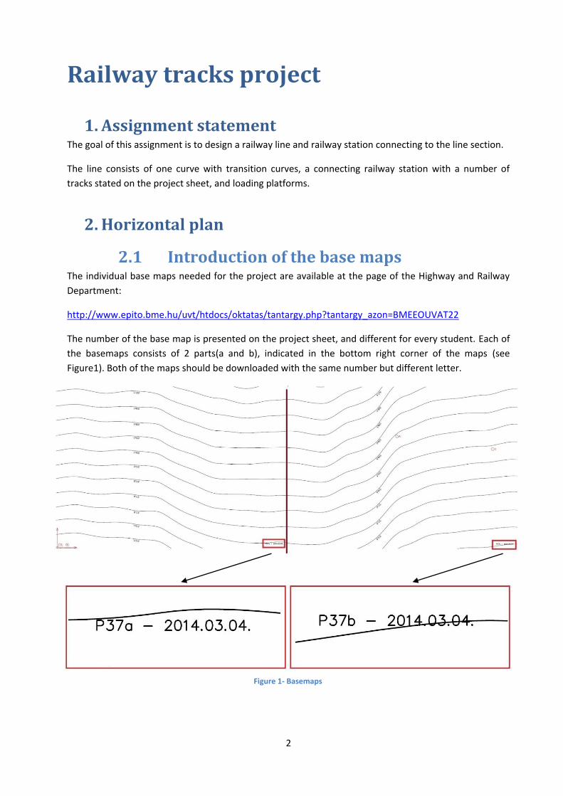
The number of the base map is presented on the project sheet, and different for every student. Each of
the basemaps consists of 2 parts(a and b), indicated in the bottom right corner of the maps (see
Figure1). Both of the maps should be downloaded with the same number but different letter.
Figure 1- Basemaps
3
The base maps are contour-maps: the lines on the map are contour lines representing the height above
sea level. The numbers on the lines indicate the height in metric unit, and the bottom of the numbers is
always towards the direction of the decrease of altitude (that is the reason they might be "upside
down").
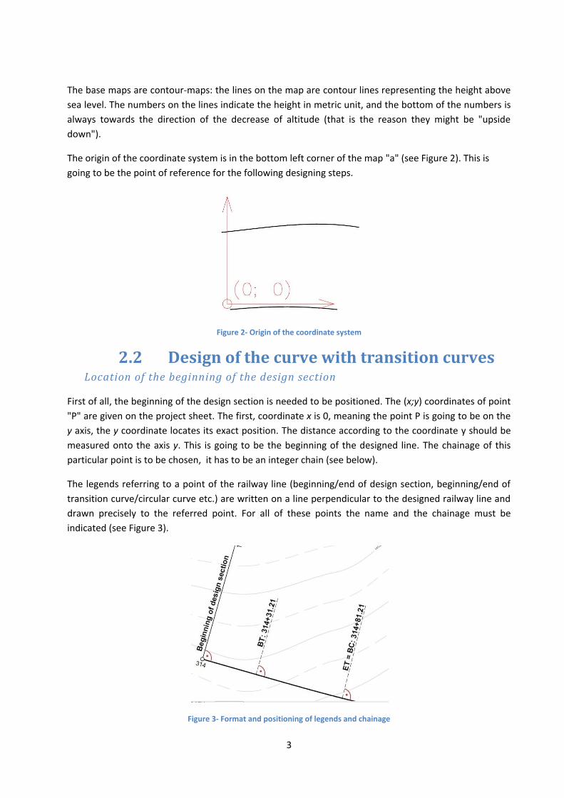
The origin of the coordinate system is in the bottom left corner of the map "a" (see Figure 2). This is
going to be the point of reference for the following designing steps.
Figure 2- Origin of the coordinate system
2.2 Design of the curve with transition curves Location of the beginning of the design section
First of all, the beginning of the design section is needed to be positioned. The (x;y) coordinates of point
"P" are given on the project sheet. The first, coordinate x is 0, meaning the point P is going to be on the
y axis, the y coordinate locates its exact position. The distance according to the coordinate y should be
measured onto the axis y. This is going to be the beginning of the designed line. The chainage of this
particular point is to be chosen, it has to be an integer chain (see below).
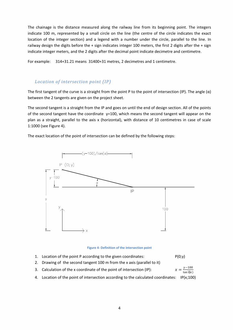
The legends referring to a point of the railway line (beginning/end of design section, beginning/end of
transition curve/circular curve etc.) are written on a line perpendicular to the designed railway line and
drawn precisely to the referred point. For all of these points the name and the chainage must be
indicated (see Figure 3).
Figure 3- Format and positioning of legends and chainage
4
The chainage is the distance measured along the railway line from its beginning point. The integers
indicate 100 m, represented by a small circle on the line (the centre of the circle indicates the exact
location of the integer section) and a legend with a number under the circle, parallel to the line. In
railway design the digits before the + sign indicates integer 100 meters, the first 2 digits after the + sign
indicate integer meters, and the 2 digits after the decimal point indicate decimetre and centimetre.
For example: 314+31.21 means 31400+31 metres, 2 decimetres and 1 centimetre.
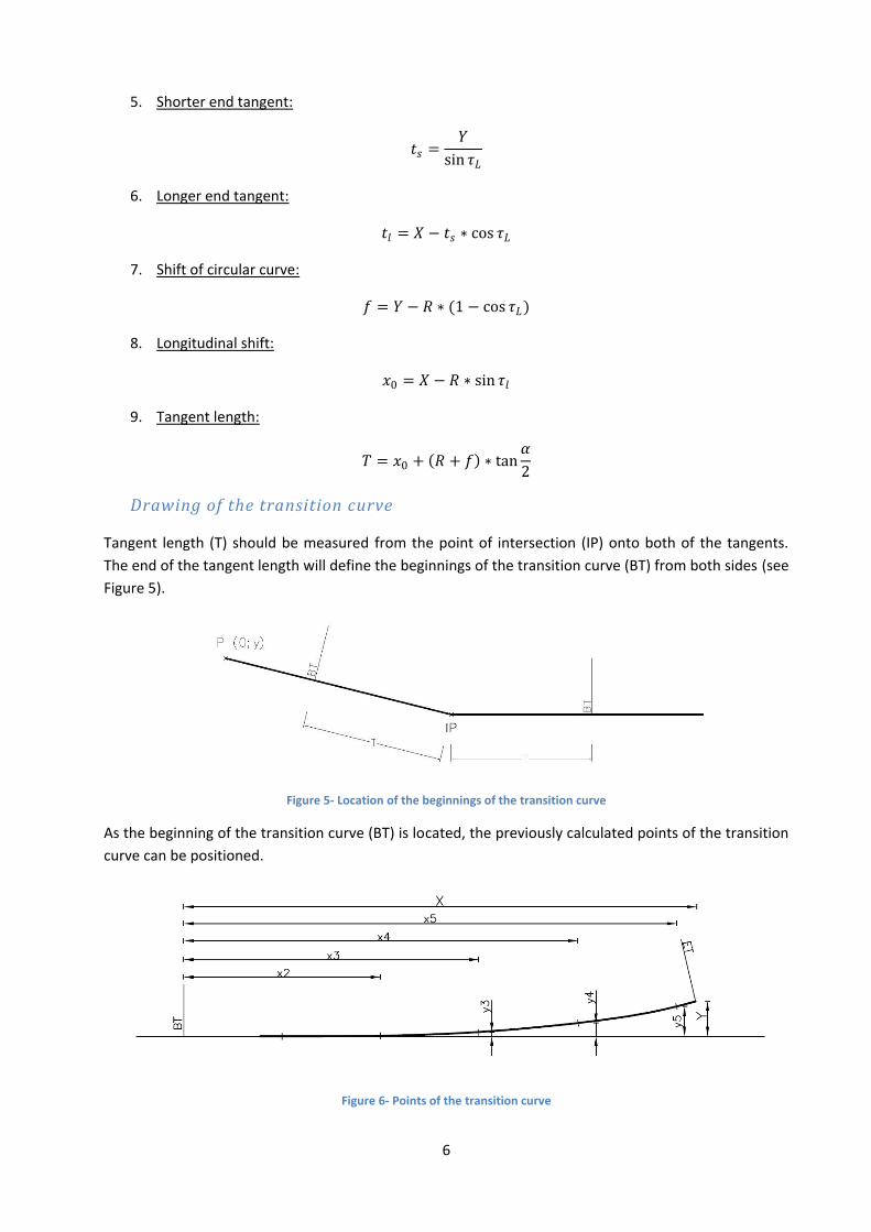
Location of intersection point (IP)
The first tangent of the curve is a straight from the point P to the point of intersection (IP). The angle (α)
between the 2 tangents are given on the project sheet.
The second tangent is a straight from the IP and goes on until the end of design section. All of the points
of the second tangent have the coordinate y=100, which means the second tangent will appear on the
plan as a straight, parallel to the axis x (horizontal), with distance of 10 centimetres in case of scale
1:1000 (see Figure 4).
The exact location of the point of intersection can be defined by the following steps:
Figure 4- Definition of the intersection point
1. Location of the point P according to the given coordinates: P(0;y)
2. Drawing of the second tangent 100 m from the x axis (parallel to it)
3. Calculation of the x coordinate of the point of intersection (IP): 𝑥 =𝑦−100
tan (𝛼)
4. Location of the point of intersection according to the calculated coordinates: IP(x;100)

5
2.2.1 Transition curve Calculations of the transition curve
1. Parameter of the clothoid transition curve, C [m2]
The parameter of the clothoid transition curve (C [m2])depends on the design speed.
Table 1- Parameter of the clothoid transition curve
2. Length of transition curve, L [m]
𝐶 = 𝑅 ∗ 𝐿 𝐿 =𝐶
𝑅
This length refers to one transition curve which means there are going to be 2 transition curves with the
length of L on both sides of the circular curve.
3. Calculation of coordinate (x;y) of detail points of the transition curve
Calculation is needed for the (x;y) coordinate of detail points every 10 m...
𝑥 = 𝑙 −𝑙5
40 ∗ 𝐶2+
𝑙9
3456 ∗ 𝐶4
𝑦 =𝑙3
6 ∗ 𝐶−
𝑙7
336 ∗ 𝐶3+
𝑙11
42240 ∗ 𝐶5
...and for the calculation of the coordinates (X;Y) of the end point (l=L):
𝑋 = 𝐿 −𝐿5
40 ∗ 𝐶2+
𝐿9
3456 ∗ 𝐶4
𝑌 =𝐿3
6 ∗ 𝐶−
𝐿7
336 ∗ 𝐶3+
𝐿11
42240 ∗ 𝐶5
4. Angle of end tangent of transition curve:
𝜏𝐿 =𝐿
2 ∗ 𝑅 [𝑟𝑎𝑑]
The equation calculates the angle in the unit of radian.
V [km/h] C [m2]
60 16800
70 27300
80 40000
90 57000
100 78000
120 135000
160 320000
6
5. Shorter end tangent:
𝑡𝑠 =𝑌
sin 𝜏𝐿
6. Longer end tangent:
𝑡𝑙 = 𝑋 − 𝑡𝑠 ∗ cos 𝜏𝐿
7. Shift of circular curve:
𝑓 = 𝑌 − 𝑅 ∗ (1 − cos 𝜏𝐿)
8. Longitudinal shift:
𝑥0 = 𝑋 − 𝑅 ∗ sin 𝜏𝑙
9. Tangent length:
𝑇 = 𝑥0 + 𝑅 + 𝑓 ∗ tan𝛼
2
Drawing of the transition curve
Tangent length (T) should be measured from the point of intersection (IP) onto both of the tangents.
The end of the tangent length will define the beginnings of the transition curve (BT) from both sides (see
Figure 5).
Figure 5- Location of the beginnings of the transition curve
As the beginning of the transition curve (BT) is located, the previously calculated points of the transition
curve can be positioned.
Figure 6- Points of the transition curve
7
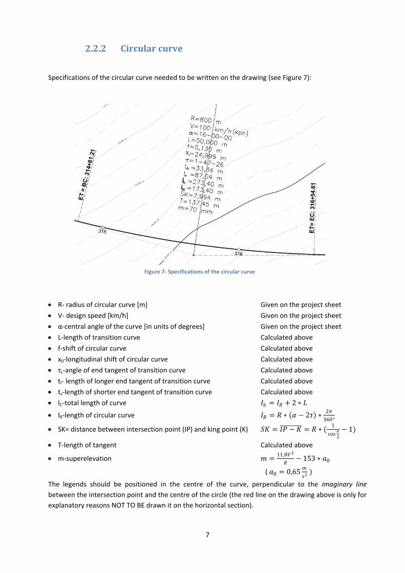
2.2.2 Circular curve
Specifications of the circular curve needed to be written on the drawing (see Figure 7):
R- radius of circular curve [m] Given on the project sheet
V- design speed [km/h] Given on the project sheet
α-central angle of the curve [in units of degrees] Given on the project sheet
L-length of transition curve Calculated above
f-shift of circular curve Calculated above
x0-longitudinal shift of circular curve Calculated above
τL-angle of end tangent of transition curve Calculated above
tl- length of longer end tangent of transition curve Calculated above
ts-length of shorter end tangent of transition curve Calculated above
IC-total length of curve 𝐼ℎ = 𝐼𝑅 + 2 ∗ 𝐿
IR-length of circular curve 𝐼𝑅 = 𝑅 ∗ 𝛼 − 2𝜏 ∗2𝜋
360°
SK= distance between intersection point (IP) and king point (K) 𝑆𝐾 = 𝐼𝑃 − 𝐾 = 𝑅 ∗ (1
cos𝛼
2
− 1)
T-length of tangent Calculated above
m-superelevation 𝑚 =11,8𝑉2
𝑅− 153 ∗ 𝑎0
( 𝑎0 = 0,65𝑚
𝑠2 )
The legends should be positioned in the centre of the curve, perpendicular to the imaginary line
between the intersection point and the centre of the circle (the red line on the drawing above is only for
explanatory reasons NOT TO BE drawn it on the horizontal section).
Figure 7- Specifications of the circular curve
8
2.3 One-alpha gathering tracks
The next part of the project to be drawn is the railway station, its connecting tracks, platforms and
facilities. The railway station consists of 3 different track types: a through track, side tracks and a
shunting track.
The through track is the straight continuation of the open line, it has been already drawn in the
previous parts of the project.
The side tracks are parallel to the through track. Track connection needs to be provided within
the railway station.
The shunting track will provide connection to the loading platforms.
The track connection in the railway station is to be drawn. The type of the track connection is one-alpha
gathering tracks, meaning that the angle of the main line and the diverging route equals to the central
deflection angle of the turnouts.
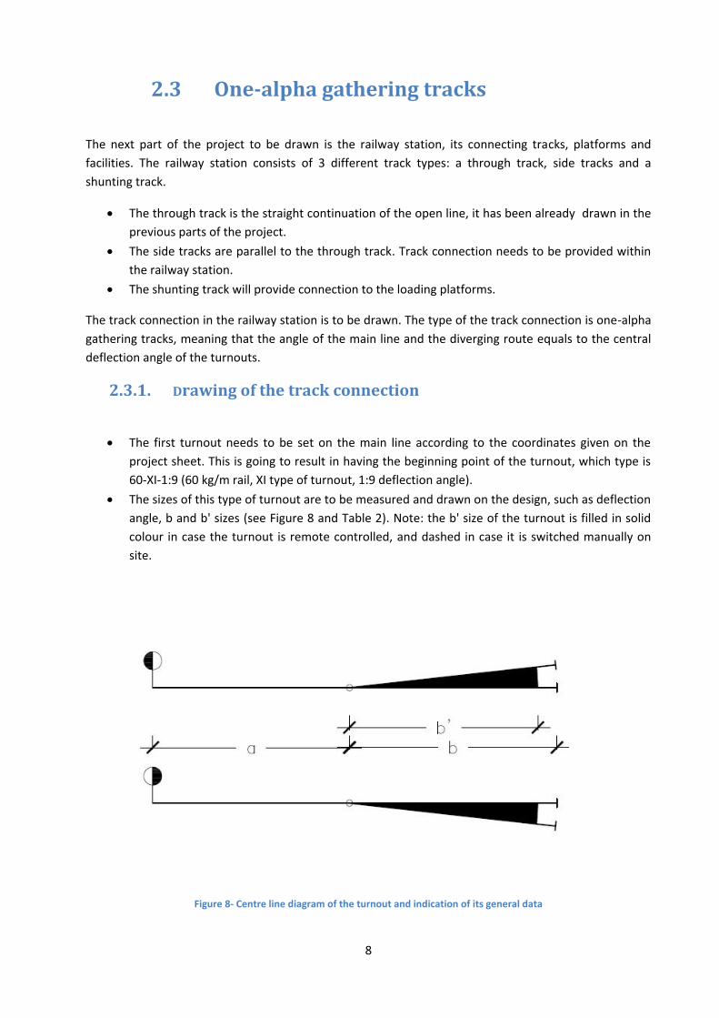
2.3.1. Drawing of the track connection
The first turnout needs to be set on the main line according to the coordinates given on the
project sheet. This is going to result in having the beginning point of the turnout, which type is
60-XI-1:9 (60 kg/m rail, XI type of turnout, 1:9 deflection angle).
The sizes of this type of turnout are to be measured and drawn on the design, such as deflection
angle, b and b' sizes (see Figure 8 and Table 2). Note: the b' size of the turnout is filled in solid
colour in case the turnout is remote controlled, and dashed in case it is switched manually on
site.
Figure 8- Centre line diagram of the turnout and indication of its general data
9
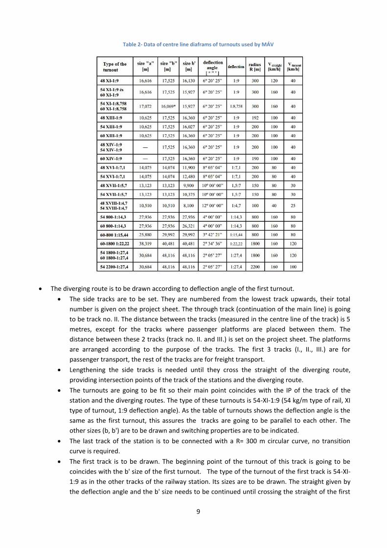
Table 2- Data of centre line diaframs of turnouts used by MÁV
The diverging route is to be drawn according to deflection angle of the first turnout.
The side tracks are to be set. They are numbered from the lowest track upwards, their total
number is given on the project sheet. The through track (continuation of the main line) is going
to be track no. II. The distance between the tracks (measured in the centre line of the track) is 5
metres, except for the tracks where passenger platforms are placed between them. The
distance between these 2 tracks (track no. II. and III.) is set on the project sheet. The platforms
are arranged according to the purpose of the tracks. The first 3 tracks (I., II., III.) are for
passenger transport, the rest of the tracks are for freight transport.
Lengthening the side tracks is needed until they cross the straight of the diverging route,
providing intersection points of the track of the stations and the diverging route.
The turnouts are going to be fit so their main point coincides with the IP of the track of the
station and the diverging routes. The type of these turnouts is 54-XI-1:9 (54 kg/m type of rail, XI
type of turnout, 1:9 deflection angle). As the table of turnouts shows the deflection angle is the
same as the first turnout, this assures the tracks are going to be parallel to each other. The
other sizes (b, b') are to be drawn and switching properties are to be indicated.
The last track of the station is to be connected with a R= 300 m circular curve, no transition
curve is required.
The first track is to be drawn. The beginning point of the turnout of this track is going to be
coincides with the b' size of the first turnout. The type of the turnout of the first track is 54-XI-
1:9 as in the other tracks of the railway station. Its sizes are to be drawn. The straight given by
the deflection angle and the b' size needs to be continued until crossing the straight of the first
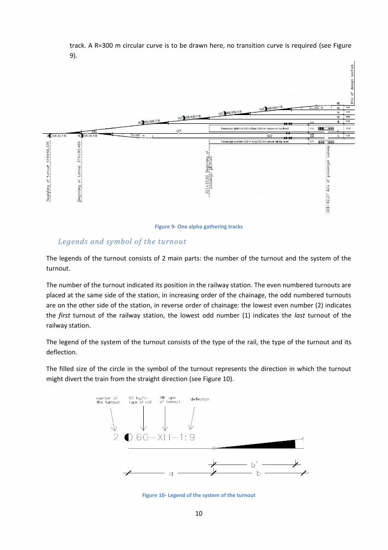
10
track. A R=300 m circular curve is to be drawn here, no transition curve is required (see Figure
9).
Figure 9- One alpha gathering tracks
Legends and symbol of the turnout
The legends of the turnout consists of 2 main parts: the number of the turnout and the system of the
turnout.
The number of the turnout indicated its position in the railway station. The even numbered turnouts are
placed at the same side of the station, in increasing order of the chainage, the odd numbered turnouts
are on the other side of the station, in reverse order of chainage: the lowest even number (2) indicates
the first turnout of the railway station, the lowest odd number (1) indicates the last turnout of the
railway station.
The legend of the system of the turnout consists of the type of the rail, the type of the turnout and its
deflection.
The filled size of the circle in the symbol of the turnout represents the direction in which the turnout
might divert the train from the straight direction (see Figure 10).
Figure 10- Legend of the system of the turnout
11
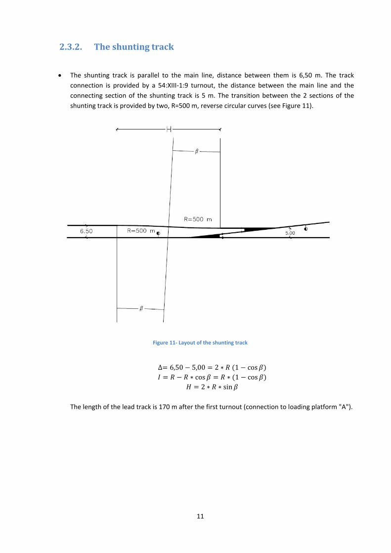
2.3.2. The shunting track
The shunting track is parallel to the main line, distance between them is 6,50 m. The track
connection is provided by a 54:XIII-1:9 turnout, the distance between the main line and the
connecting section of the shunting track is 5 m. The transition between the 2 sections of the
shunting track is provided by two, R=500 m, reverse circular curves (see Figure 11).
∆= 6,50 − 5,00 = 2 ∗ 𝑅 (1 − cos 𝛽)
𝐼 = 𝑅 − 𝑅 ∗ cos 𝛽 = 𝑅 ∗ (1 − cos 𝛽)
𝐻 = 2 ∗ 𝑅 ∗ sin 𝛽
The length of the lead track is 170 m after the first turnout (connection to loading platform "A").
Figure 11- Layout of the shunting track
12
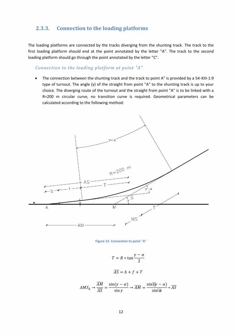
2.3.3. Connection to the loading platforms
The loading platforms are connected by the tracks diverging from the shunting track. The track to the
first loading platform should end at the point annotated by the letter "A". The track to the second
loading platform should go through the point annotated by the letter "C".
Connection to the loading platform at point "A"
The connection between the shunting track and the track to point A" is provided by a 54-XIII-1:9
type of turnout. The angle (γ) of the straight from point "A" to the shunting track is up to your
choice. The diverging route of the turnout and the straight from point "A" is to be linked with a
R=200 m circular curve, no transition curve is required. Geometrical parameters can be
calculated according to the following method:
Figure 12- Connection to point "A"
𝑇 = 𝑅 ∗ tan𝛾 − 𝛼
2
𝐴𝑆 = 𝑏 + 𝑓 + 𝑇
𝐴𝑀𝑆∆ →𝐴𝑀
𝐴𝑆 =
sin(𝛾 − 𝛼)
sin 𝛾→ 𝐴𝑀 =
sin(𝛾 − 𝛼)
sin𝛼∗ 𝐴𝑆
13
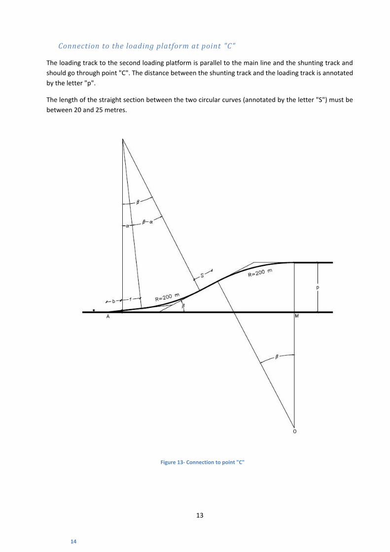
Connection to the loading platform at point "C"
The loading track to the second loading platform is parallel to the main line and the shunting track and
should go through point "C". The distance between the shunting track and the loading track is annotated
by the letter "p".
The length of the straight section between the two circular curves (annotated by the letter "S") must be
between 20 and 25 metres.
14
Figure 13- Connection to point "C"
14
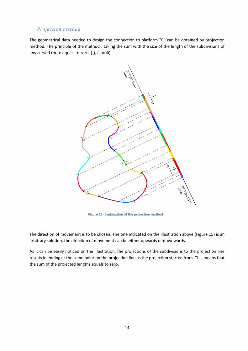
Projection method
The geometrical data needed to design the connection to platform "C" can be obtained by projection
method. The principle of the method : taking the sum with the size of the length of the subdivisions of
any curved route equals to zero. ( 𝑙𝑖 = ∅)
The direction of movement is to be chosen. The one indicated on the illustration above (Figure 15) is an
arbitrary solution, the direction of movement can be either upwards or downwards.
As it can be easily noticed on the illustration, the projections of the subdivisions to the projection line
results in ending at the same point on the projection line as the projection started from. This means that
the sum of the projected lengths equals to zero.
Figure 15- Explanation of the projection method

15
Projection method in use of connection to platform " C"
Projection equation:
𝐛 + 𝐟 ∗ 𝐬𝐢𝐧 𝛂 + 𝐑 ∗ (𝐜𝐨𝐬𝛂 − 𝐜𝐨𝐬 𝛃) + 𝐒 ∗ 𝐬𝐢𝐧 𝛃 + R ∗ (1 − cos β) − p = ∅
After having the equation solved, angle "β" ( ° ' ") can be obtained.
Figure 16- Projection method in use of connection to point "C"
16
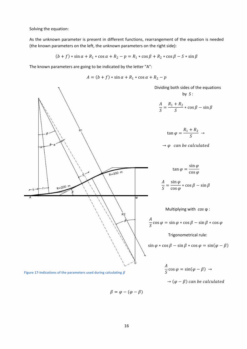
Solving the equation:
As the unknown parameter is present in different functions, rearrangement of the equation is needed
(the known parameters on the left, the unknown parameters on the right side):
𝑏 + 𝑓 ∗ sin 𝛼 + 𝑅1 ∗ cos 𝛼 + 𝑅2 − 𝑝 = 𝑅1 ∗ cos 𝛽 + 𝑅2 ∗ cos 𝛽 − 𝑆 ∗ sin 𝛽
The known parameters are going to be indicated by the letter "A":
𝐴 = 𝑏 + 𝑓 ∗ sin 𝛼 + 𝑅1 ∗ cos 𝛼 + 𝑅2 − 𝑝
Dividing both sides of the equations
by S :
𝐴
𝑆=
𝑅1 + 𝑅2
𝑆∗ cos 𝛽 − sin 𝛽
tan 𝜑 =𝑅1 + 𝑅2
𝑆 →
→ 𝜑 𝑐𝑎𝑛 𝑏𝑒 𝑐𝑎𝑙𝑐𝑢𝑙𝑎𝑡𝑒𝑑
tan 𝜑 =sin 𝜑
cos 𝜑
𝐴
𝑆=
sin 𝜑
cos 𝜑∗ cos 𝛽 − sin 𝛽
Multiplying with cos ϕ :
𝐴
𝑆cos 𝜑 = sin 𝜑 ∗ cos 𝛽 − sin 𝛽 ∗ cos 𝜑
Trigonometrical rule:
sin 𝜑 ∗ cos 𝛽 − sin 𝛽 ∗ cos 𝜑 = sin 𝜑 − 𝛽
𝐴
𝑆cos 𝜑 = sin 𝜑 − 𝛽 →
→ 𝜑 − 𝛽 𝑐𝑎𝑛 𝑏𝑒 𝑐𝑎𝑙𝑐𝑢𝑙𝑎𝑡𝑒𝑑
𝛽 = 𝜑 − (𝜑 − 𝛽)
Figure 17-Indications of the parameters used during calculating 𝜷
17
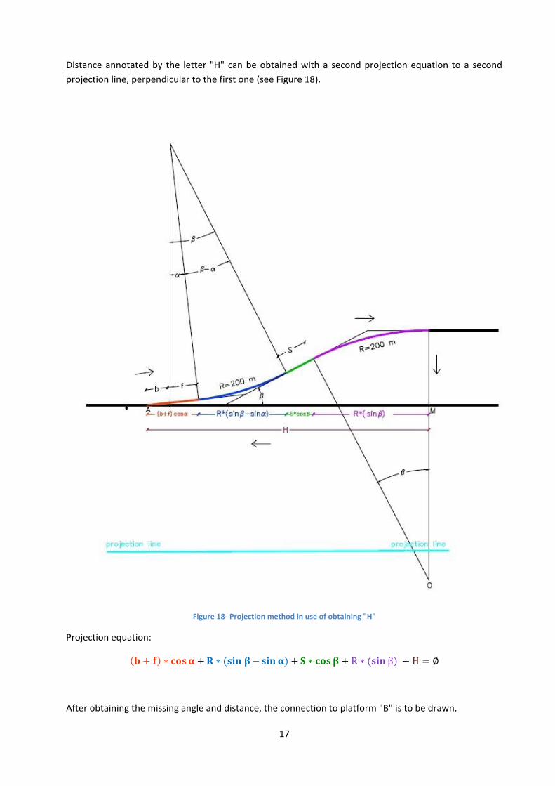
Distance annotated by the letter "H" can be obtained with a second projection equation to a second
projection line, perpendicular to the first one (see Figure 18).
Figure 18- Projection method in use of obtaining "H"
Projection equation:
𝐛 + 𝐟 ∗ 𝐜𝐨𝐬𝛂 + 𝐑 ∗ (𝐬𝐢𝐧 𝛃−𝐬𝐢𝐧 𝛂) + 𝐒 ∗ 𝐜𝐨𝐬𝛃 + R ∗ (𝐬𝐢𝐧 β) − H = ∅
After obtaining the missing angle and distance, the connection to platform "B" is to be drawn.
18
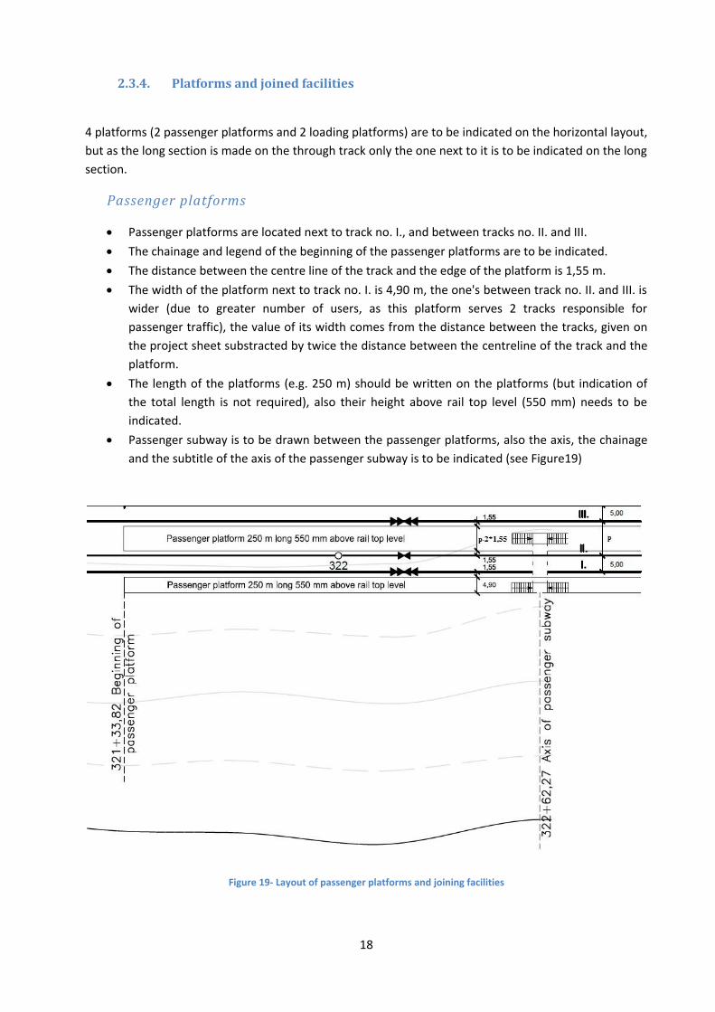
2.3.4. Platforms and joined facilities
4 platforms (2 passenger platforms and 2 loading platforms) are to be indicated on the horizontal layout,
but as the long section is made on the through track only the one next to it is to be indicated on the long
section.
Passenger platforms
Passenger platforms are located next to track no. I., and between tracks no. II. and III.
The chainage and legend of the beginning of the passenger platforms are to be indicated.
The distance between the centre line of the track and the edge of the platform is 1,55 m.
The width of the platform next to track no. I. is 4,90 m, the one's between track no. II. and III. is
wider (due to greater number of users, as this platform serves 2 tracks responsible for
passenger traffic), the value of its width comes from the distance between the tracks, given on
the project sheet substracted by twice the distance between the centreline of the track and the
platform.
The length of the platforms (e.g. 250 m) should be written on the platforms (but indication of
the total length is not required), also their height above rail top level (550 mm) needs to be
indicated.
Passenger subway is to be drawn between the passenger platforms, also the axis, the chainage
and the subtitle of the axis of the passenger subway is to be indicated (see Figure19)
Figure 19- Layout of passenger platforms and joining facilities
19
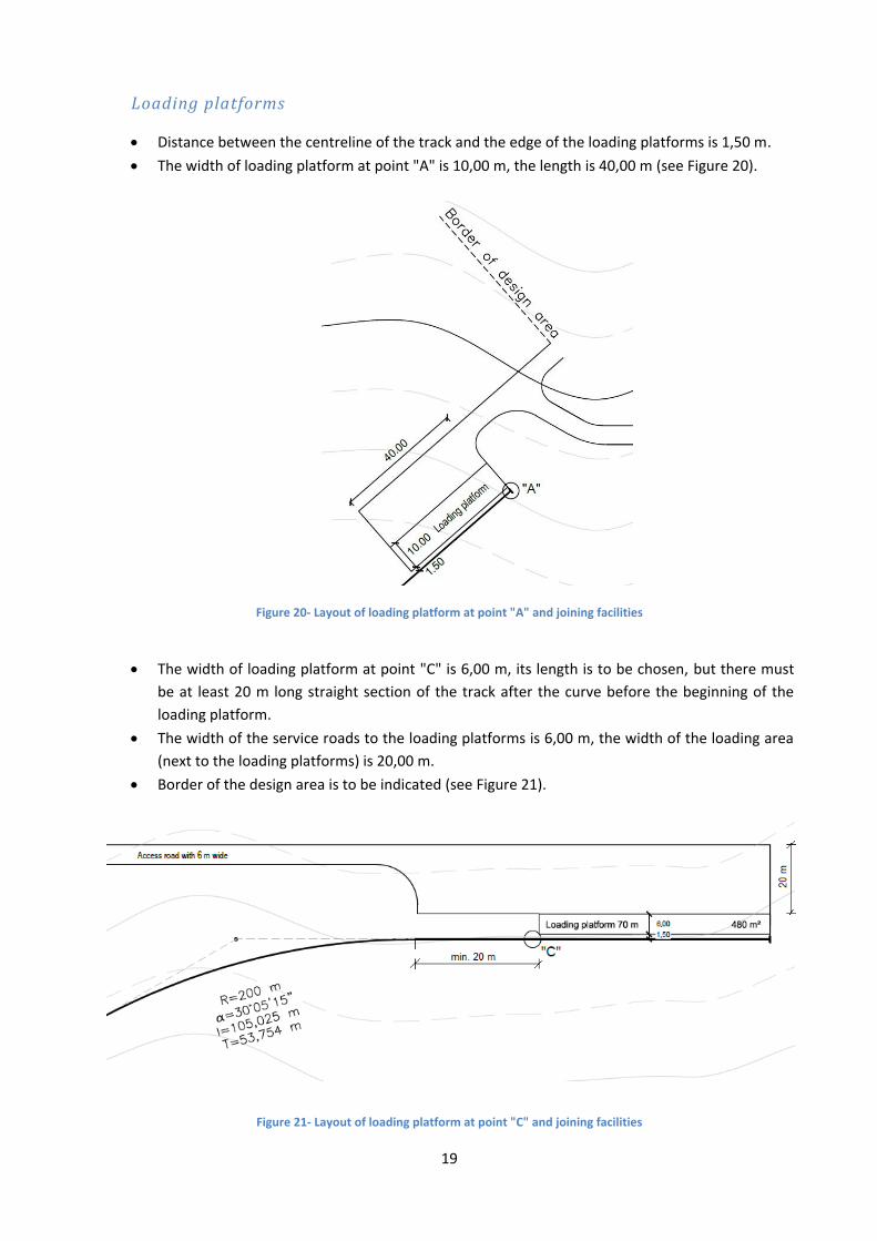
Loading platforms
Distance between the centreline of the track and the edge of the loading platforms is 1,50 m.
The width of loading platform at point "A" is 10,00 m, the length is 40,00 m (see Figure 20).
Figure 20- Layout of loading platform at point "A" and joining facilities
The width of loading platform at point "C" is 6,00 m, its length is to be chosen, but there must
be at least 20 m long straight section of the track after the curve before the beginning of the
loading platform.
The width of the service roads to the loading platforms is 6,00 m, the width of the loading area
(next to the loading platforms) is 20,00 m.
Border of the design area is to be indicated (see Figure 21).
Figure 21- Layout of loading platform at point "C" and joining facilities
20
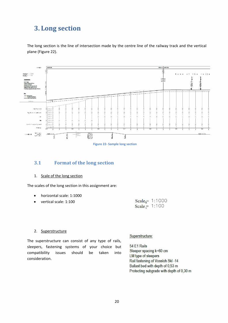
3. Long section
The long section is the line of intersection made by the centre line of the railway track and the vertical
plane (Figure 22).
3.1 Format of the long section
1. Scale of the long section
The scales of the long section in this assignment are:
horizontal scale: 1:1000
vertical scale: 1:100
2. Superstructure
The superstructure can consist of any type of rails,
sleepers, fastening systems of your choice but
compatibility issues should be taken into
consideration.
Figure 22- Sample long section
21
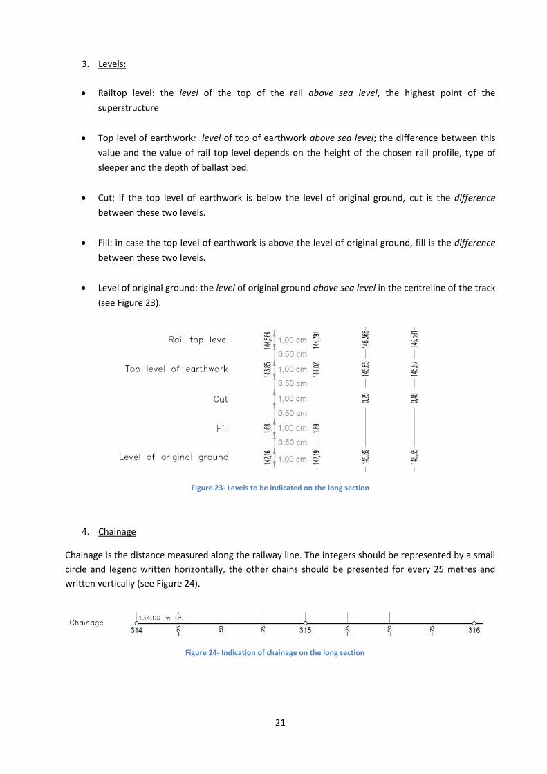
3. Levels:
Railtop level: the level of the top of the rail above sea level, the highest point of the
superstructure
Top level of earthwork: level of top of earthwork above sea level; the difference between this
value and the value of rail top level depends on the height of the chosen rail profile, type of
sleeper and the depth of ballast bed.
Cut: If the top level of earthwork is below the level of original ground, cut is the difference
between these two levels.
Fill: in case the top level of earthwork is above the level of original ground, fill is the difference
between these two levels.
Level of original ground: the level of original ground above sea level in the centreline of the track
(see Figure 23).
Figure 23- Levels to be indicated on the long section
4. Chainage
Chainage is the distance measured along the railway line. The integers should be represented by a small
circle and legend written horizontally, the other chains should be presented for every 25 metres and
written vertically (see Figure 24).
Figure 24- Indication of chainage on the long section
22
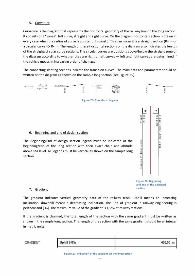
5. Curvature
Curvature is the diagram that represents the horizontal geometry of the railway line on the long section.
It consists of 3 "zones": left curve, straight and right curve. On the diagram horizontal section is drawn in
every case when the radius of curve is constant (R=const.). This can mean it is a straight section (R=∞) or
a circular curve (0<R<∞). The length of these horizontal sections on the diagram also indicates the length
of the straight/circular curve sections. The circular curves are positions above/below the straight zone of
the diagram according to whether they are right or left curves — left and right curves are determined if
the vehicle moves in increasing order of chainage.
The connecting slanting sections indicate the transition curves. The main data and parameters should be
written on the diagram as shown on the sample long section (see Figure 25).
Figure 25- Curvature diagram
6. Beginning and end of design section
The Beginning/End of design section legend must be indicated at the
beginning/end of the long section with their exact chain and altitude
above sea level. All legends must be vertical as shown on the sample long
section.
7. Gradient
The gradient indicates vertical geometry data of the railway track. Uphill means an increasing
inclination, downhill means a decreasing inclination. The unit of gradient in railway engineering is
perthousand [‰]. The maximum value of the gradient is 1,5‰ at railway stations.
If the gradient is changed, the total length of the section with the same gradient must be written as
shown in the sample long section. This length of the section with the same gradient should be an integer
in metric units.
Figure 26- Beginning and end of the designed section
Figure 27- Indication of the gradient on the long section
23
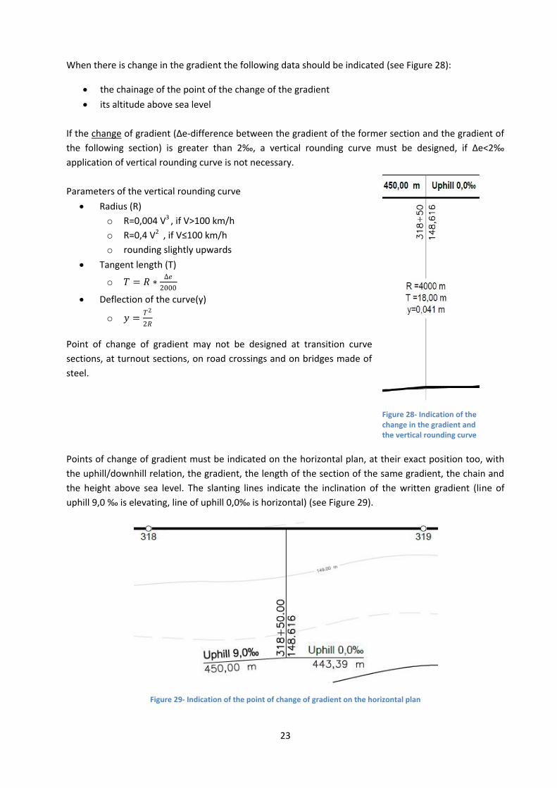
When there is change in the gradient the following data should be indicated (see Figure 28):
the chainage of the point of the change of the gradient
its altitude above sea level
If the change of gradient (Δe-difference between the gradient of the former section and the gradient of
the following section) is greater than 2‰, a vertical rounding curve must be designed, if Δe<2‰
application of vertical rounding curve is not necessary.
Parameters of the vertical rounding curve
Radius (R)
o R=0,004 V3 , if V>100 km/h
o R=0,4 V2 , if V≤100 km/h
o rounding slightly upwards
Tangent length (T)
o 𝑇 = 𝑅 ∗∆𝑒
2000
Deflection of the curve(y)
o 𝑦 =𝑇2
2𝑅
Point of change of gradient may not be designed at transition curve
sections, at turnout sections, on road crossings and on bridges made of
steel.
Points of change of gradient must be indicated on the horizontal plan, at their exact position too, with
the uphill/downhill relation, the gradient, the length of the section of the same gradient, the chain and
the height above sea level. The slanting lines indicate the inclination of the written gradient (line of
uphill 9,0 ‰ is elevating, line of uphill 0,0‰ is horizontal) (see Figure 29).
Figure 29- Indication of the point of change of gradient on the horizontal plan
Figure 28- Indication of the change in the gradient and the vertical rounding curve
24
3.2 Drawing of the long section
After the "frame" of the long section is drawn, the following steps are to be done:
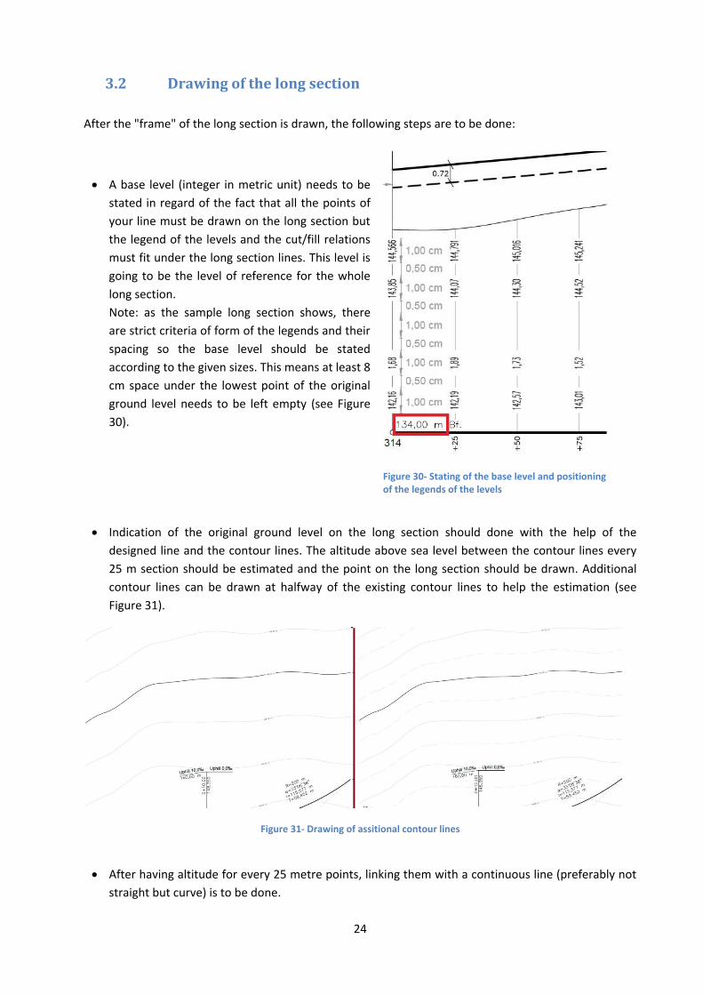
A base level (integer in metric unit) needs to be
stated in regard of the fact that all the points of
your line must be drawn on the long section but
the legend of the levels and the cut/fill relations
must fit under the long section lines. This level is
going to be the level of reference for the whole
long section.
Note: as the sample long section shows, there
are strict criteria of form of the legends and their
spacing so the base level should be stated
according to the given sizes. This means at least 8
cm space under the lowest point of the original
ground level needs to be left empty (see Figure
30).
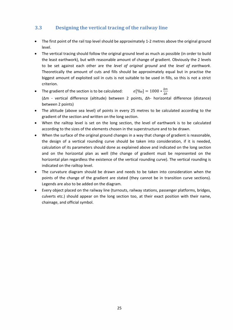
Indication of the original ground level on the long section should done with the help of the
designed line and the contour lines. The altitude above sea level between the contour lines every
25 m section should be estimated and the point on the long section should be drawn. Additional
contour lines can be drawn at halfway of the existing contour lines to help the estimation (see
Figure 31).
Figure 31- Drawing of assitional contour lines
After having altitude for every 25 metre points, linking them with a continuous line (preferably not
straight but curve) is to be done.
Figure 30- Stating of the base level and positioning of the legends of the levels
25
3.3 Designing the vertical tracing of the railway line
The first point of the rail top level should be approximately 1-2 metres above the original ground
level.
The vertical tracing should follow the original ground level as much as possible (in order to build
the least earthwork), but with reasonable amount of change of gradient. Obviously the 2 levels
to be set against each other are the level of original ground and the level of earthwork.
Theoretically the amount of cuts and fills should be approximately equal but in practise the
biggest amount of exploited soil in cuts is not suitable to be used in fills, so this is not a strict
criterion.
The gradient of the section is to be calculated: 𝑒[‰] = 1000 ∗∆𝑚
∆ℎ
(Δm - vertical difference (altitude) between 2 points, Δh- horizontal difference (distance)
between 2 points)
The altitude (above sea level) of points in every 25 metres to be calculated according to the
gradient of the section and written on the long section.
When the railtop level is set on the long section, the level of earthwork is to be calculated
according to the sizes of the elements chosen in the superstructure and to be drawn.
When the surface of the original ground changes in a way that change of gradient is reasonable,
the design of a vertical rounding curve should be taken into consideration, if it is needed,
calculation of its parameters should done as explained above and indicated on the long section
and on the horizontal plan as well (the change of gradient must be represented on the
horizontal plan regardless the existence of the vertical rounding curve). The vertical rounding is
indicated on the railtop level.
The curvature diagram should be drawn and needs to be taken into consideration when the
points of the change of the gradient are stated (they cannot be in transition curve sections).
Legends are also to be added on the diagram.
Every object placed on the railway line (turnouts, railway stations, passenger platforms, bridges,
culverts etc.) should appear on the long section too, at their exact position with their name,
chainage, and official symbol.
26
List of Figures and Tables
Figure 1- Basemaps ...................................................................................................................................... 2
Figure 2- Origin of the coordinate system.................................................................................................... 3
Figure 3- Format and positioning of legends and chainage ......................................................................... 3
Figure 4- Definition of the intersection point .............................................................................................. 4
Figure 5- Location of the beginnings of the transition curve ....................................................................... 6
Figure 6- Points of the transition curve ........................................................................................................ 6
Figure 7- Specifications of the circular curve ............................................................................................... 7
Figure 8- Centre line diagram of the turnout and indication of its general data ......................................... 8
Figure 9- One alpha gathering tracks ......................................................................................................... 10
Figure 10- Legend of the system of the turnout ........................................................................................ 10
Figure 11- Layout of the shunting track ..................................................................................................... 11
Figure 12- Connection to point "A" ............................................................................................................ 12
Figure 13- Connection to point "C" ............................................................................................................ 13
Figure 15- Explanation of the projection method ...................................................................................... 14
Figure 16- Projection method in use of connection to point "C" ............................................................... 15
Figure 17-Indications of the parameters used during calculating 𝛽 .......................................................... 16
Figure 18- Projection method in use of obtaining "H" ............................................................................... 17
Figure 19- Layout of passenger platforms and joining facilities ................................................................ 18
Figure 20- Layout of loading platform at point "A" and joining facilities ................................................... 19
Figure 21- Layout of loading platform at point "C" and joining facilities ................................................... 19
Figure 22- Sample long section .................................................................................................................. 20
Figure 23- Levels to be indicated on the long section ................................................................................ 21
Figure 24- Indication of chainage on the long section ............................................................................... 21
Figure 25- Curvature diagram .................................................................................................................... 22
Figure 26- Beginning and end of the designed section .............................................................................. 22
Figure 27- Indication of the gradient on the long section .......................................................................... 22
Figure 29- Indication of the point of change of gradient on the horizontal plan ...................................... 23
Figure 28- Indication of the change in the gradient and the vertical rounding curve ............................... 23
Figure 31- Drawing of assitional contour lines ........................................................................................... 24
Figure 30- Stating of the base level and positioning of the legends of the levels...................................... 24
Table 1- Parameter of the clothoid transition curve .................................................................................... 5
Table 2- Data of centre line diaframs of turnouts used by MÁV ................................................................. 9
27
Table of contents
1. Assignment statement ......................................................................................................................... 2
2. Horizontal plan ..................................................................................................................................... 2
2.1 Introduction of the base maps ..................................................................................................... 2
2.2 Design of the curve with transition curves ................................................................................... 3
Location of the beginning of the design section .............................................................................. 3
Location of intersection point (IP) .................................................................................................... 4
2.2.1 Transition curve .................................................................................................................... 5
Calculations of the transition curve ................................................................................................. 5
Drawing of the transition curve ....................................................................................................... 6
2.2.2 Circular curve ........................................................................................................................ 7
2.3 One-alpha gathering tracks .......................................................................................................... 8
2.3.1. Drawing of the track connection .......................................................................................... 8
Legends and symbol of the turnout ............................................................................................... 10
2.3.2. The shunting track .............................................................................................................. 11
2.3.3. Connection to the loading platforms ................................................................................. 12
Connection to the loading platform at point "A" ........................................................................... 12
Connection to the loading platform at point "C" ........................................................................... 13
Projection method .......................................................................................................................... 14
Projection method in use of connection to platform "C" .............................................................. 15
2.3.4. Platforms and joined facilities ............................................................................................ 18
Passenger platforms ....................................................................................................................... 18
Loading platforms ........................................................................................................................... 19
3. Long section ........................................................................................................................................ 20
3.1 Format of the long section ......................................................................................................... 20
3.2 Drawing of the long section ....................................................................................................... 24
3.3 Designing the vertical tracing of the railway line ....................................................................... 25
List of Figures and Tables ........................................................................................................................... 26