Radio Telescopes and Interferometry

Instrumentation Class Nov. 29, 2007

Radio Telescopesand

Interferometry


Radio Telescopes: Some Technical Aspects• Radio Telescope: - Consists of two main components - Telescope (antenna) itself with control system - Receiver plus associated detection electronics• Antenna: 1) Input impedence - a measure of how efficiently signal transformed into a wave 2) Polarization 3) Power pattern or gain function g(θ, φ) 4) Effective area Ae (θ,φ) where g(θ,φ) = 4π/λ2Ae

TA = 1/4π g(θ,φ) TB (θ,φ) dΩ = Antenna Temperature: convolution of source andantenna properties - imbed antenna in Blackbody at T TA = T/4π g(θ,φ) dΩ = T

∫

∫


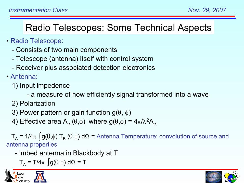
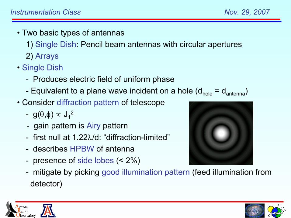
• Two basic types of antennas 1) Single Dish: Pencil beam antennas with circular apertures 2) Arrays• Single Dish - Produces electric field of uniform phase - Equivalent to a plane wave incident on a hole (dhole = dantenna)• Consider diffraction pattern of telescope - g(θ,φ) ∝ J1

2

- gain pattern is Airy pattern - first null at 1.22λ/d: “diffraction-limited” - describes HPBW of antenna - presence of side lobes (< 2%) - mitigate by picking good illumination pattern (feed illumination from detector)


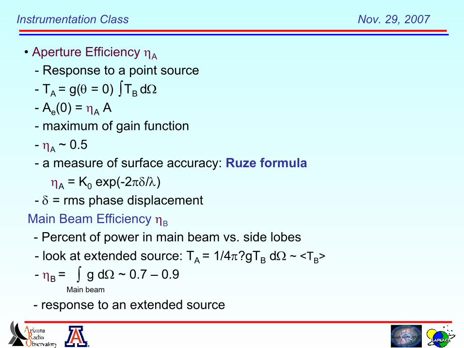
• Aperture Efficiency ηA

- Response to a point source - TA = g(θ = 0) TB dΩ - Ae(0) = ηA A - maximum of gain function - ηA ~ 0.5 - a measure of surface accuracy: Ruze formula

ηA = K0 exp(-2πδ/λ) - δ = rms phase displacement Main Beam Efficiency ηB

- Percent of power in main beam vs. side lobes - look at extended source: TA = 1/4π? gTB dΩ ~ <TB> - ηB = g dΩ ~ 0.7 – 0.9

- response to an extended sourceMain beam

∫

∫


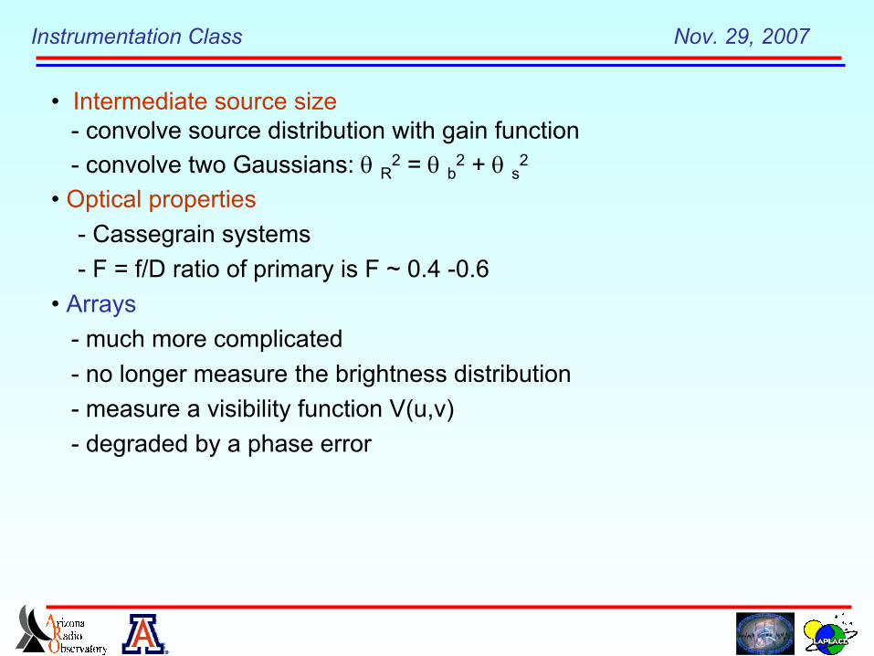
• Intermediate source size - convolve source distribution with gain function - convolve two Gaussians: θ R2 = θ b2 + θ s2

• Optical properties - Cassegrain systems - F = f/D ratio of primary is F ~ 0.4 -0.6• Arrays - much more complicated - no longer measure the brightness distribution - measure a visibility function V(u,v) - degraded by a phase error



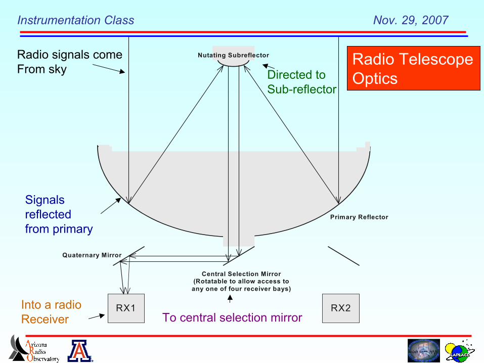
RX1 RX2

Nutating Subreflector

Primary Reflector

Quaternary Mirror

Central Selection Mirror(Rotatable to allow access toany one of four receiver bays)

Radio signals comeFrom sky

Signalsreflectedfrom primary

Radio TelescopeOpticsDirected to

Sub-reflector

To central selection mirrorInto a radioReceiver


DewarwindowLens

Feedhorn

Coupler

Mixer

Bias

Isolator

HEMTamplifier

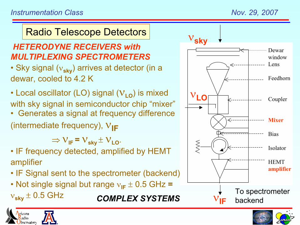
HETERODYNE RECEIVERS withMULTIPLEXING SPECTROMETERS• Sky signal (νsky) arrives at detector (in adewar, cooled to 4.2 K

• Local oscillator (LO) signal (νLO) is mixedwith sky signal in semiconductor chip “mixer”• Generates a signal at frequency difference(intermediate frequency), νIF ⇒ νIF = νsky ± νLO.• IF frequency detected, amplified by HEMTamplifier• IF Signal sent to the spectrometer (backend)• Not single signal but range νIF ± 0.5 GHz =νsky ± 0.5 GHz

Radio Telescope Detectors

νLO

νsky

νIFTo spectrometerbackendCOMPLEX SYSTEMS


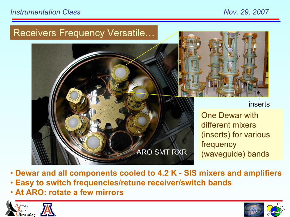
• Dewar and all components cooled to 4.2 K - SIS mixers and amplifiers• Easy to switch frequencies/retune receiver/switch bands• At ARO: rotate a few mirrors

Receivers Frequency Versatile…

One Dewar withdifferent mixers(inserts) for variousfrequency(waveguide) bandsARO SMT RXR

inserts



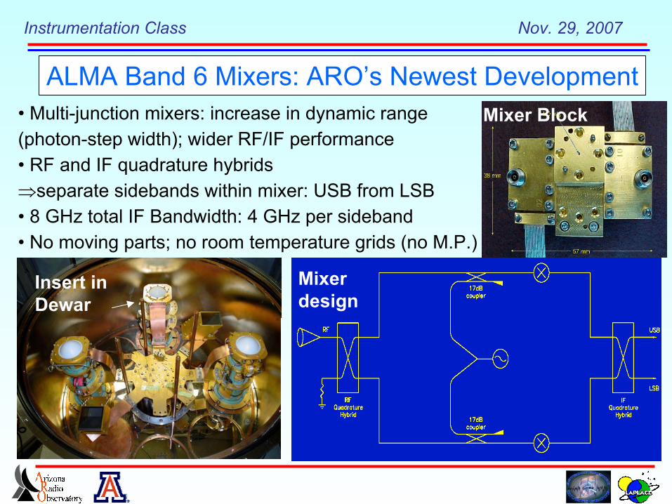
• Multi-junction mixers: increase in dynamic range(photon-step width); wider RF/IF performance• RF and IF quadrature hybrids⇒separate sidebands within mixer: USB from LSB• 8 GHz total IF Bandwidth: 4 GHz per sideband• No moving parts; no room temperature grids (no M.P.)

ALMA Band 6 Mixers: ARO’s Newest DevelopmentMixer Block

Insert in Dewar

Mixerdesign


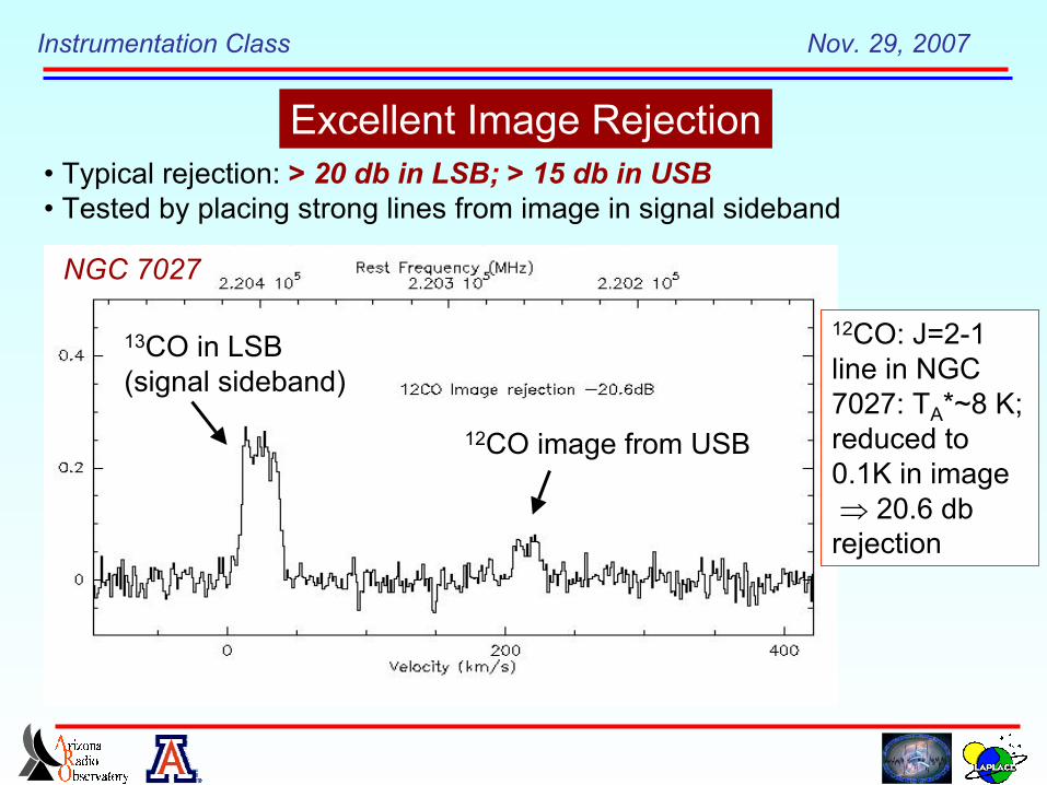
Excellent Image Rejection• Typical rejection: > 20 db in LSB; > 15 db in USB• Tested by placing strong lines from image in signal sideband

13CO in LSB (signal sideband)

12CO image from USB

NGC 7027

12CO: J=2-1line in NGC7027: TA*~8 K;reduced to0.1K in image ⇒ 20.6 dbrejection


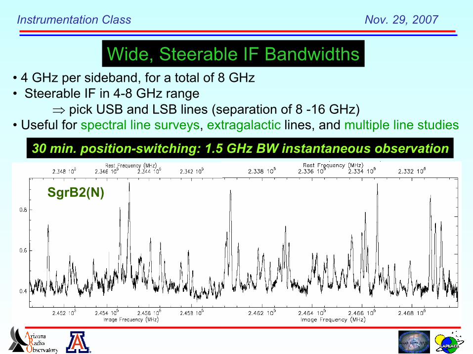
• 4 GHz per sideband, for a total of 8 GHz• Steerable IF in 4-8 GHz range ⇒ pick USB and LSB lines (separation of 8 -16 GHz)• Useful for spectral line surveys, extragalactic lines, and multiple line studies

30 min. position-switching: 1.5 GHz BW instantaneous observation

Wide, Steerable IF Bandwidths

SgrB2(N)


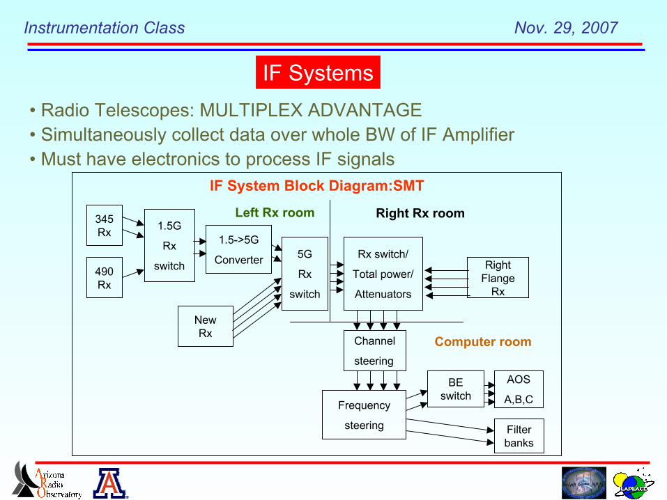
IF Systems• Radio Telescopes: MULTIPLEX ADVANTAGE• Simultaneously collect data over whole BW of IF Amplifier• Must have electronics to process IF signals

Frequency

steering

AOS

A,B,C

Filterbanks

Rx switch/

Total power/

Attenuators

IF System Block Diagram:SMT

Channel

steering

345Rx

490Rx

NewRx

1.5G

Rx

switch RightFlange

Rx

BEswitch

1.5->5G

Converter 5G

Rx

switch

Right Rx roomLeft Rx room

Computer room


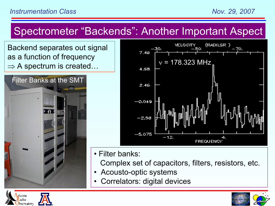
Spectrometer “Backends”: Another Important Aspect

• Filter banks: Complex set of capacitors, filters, resistors, etc.• Acousto-optic systems• Correlators: digital devices

Backend separates out signalas a function of frequency⇒ A spectrum is created… ν = 178.323 MHz

Filter Banks at the SMT


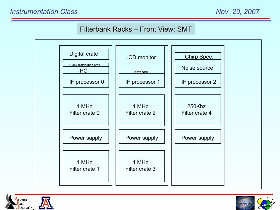
Filterbank Racks – Front View: SMT

Power supply

IF processor 0

PC

Digital crate

1 MHzFilter crate 0

Power supply

IF processor 1

LCD monitor

Power supply

IF processor 2

Chirp Spec.

Noise source

250KhzFilter crate 4

Clock distribution amp

Keyboard

1 MHzFilter crate 2

1 MHzFilter crate 1

1 MHzFilter crate 3


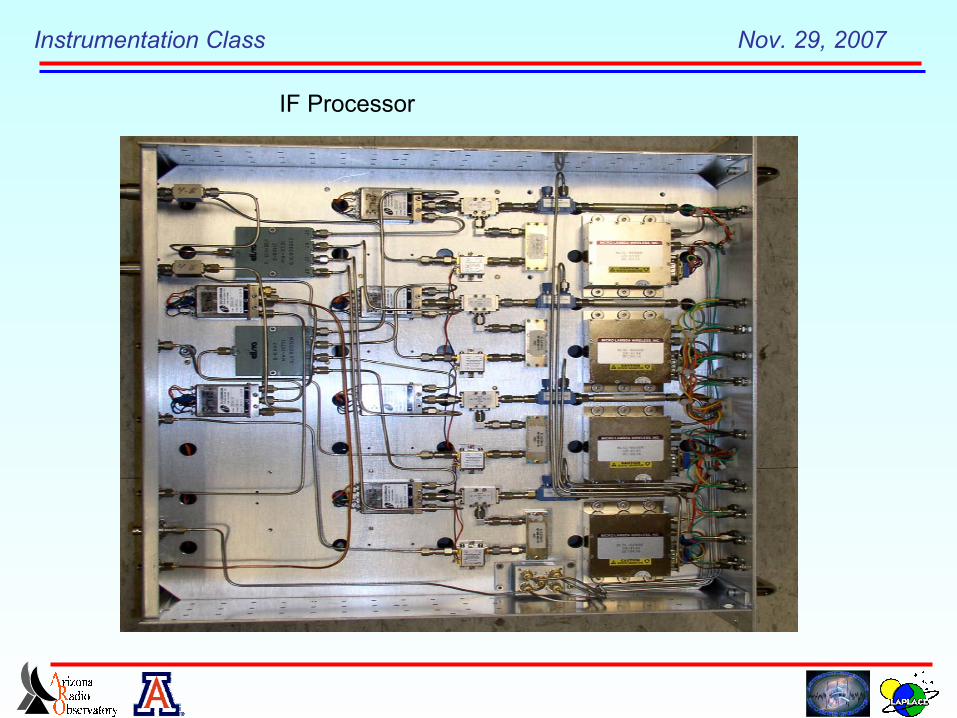
IF Processor


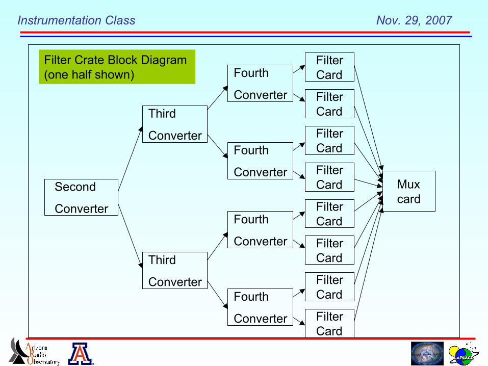
Filter Crate Block Diagram (one half shown)

Second

Converter

Third

Converter

Fourth

Converter

MuxcardFilter

Card

Fourth

Converter

FilterCard

FilterCard

FilterCard

Third

Converter

Fourth

Converter

FilterCard

Fourth

Converter

FilterCard

FilterCard

FilterCard


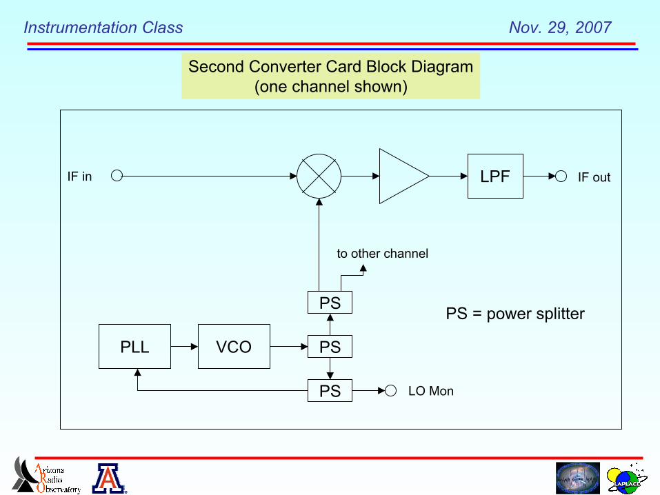
LPF

Second Converter Card Block Diagram(one channel shown)

VCOPLL PS

PS

PS

LO Mon

IF in IF out

to other channel

PS = power splitter


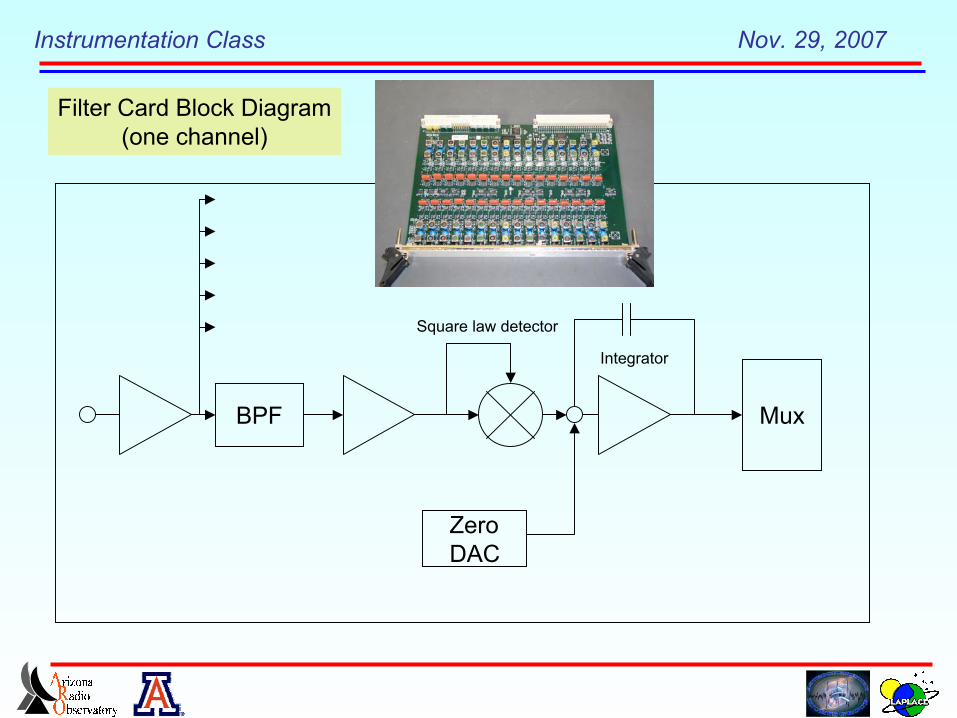
Mux

Filter Card Block Diagram(one channel)

BPF

ZeroDAC

Square law detector

Integrator


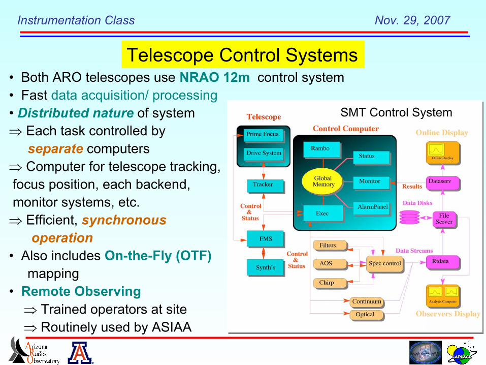
Telescope Control Systems• Both ARO telescopes use NRAO 12m control system• Fast data acquisition/ processing• Distributed nature of system⇒ Each task controlled by separate computers ⇒ Computer for telescope tracking, focus position, each backend, monitor systems, etc.⇒ Efficient, synchronous operation• Also includes On-the-Fly (OTF) mapping• Remote Observing ⇒ Trained operators at site ⇒ Routinely used by ASIAA

SMT Control System


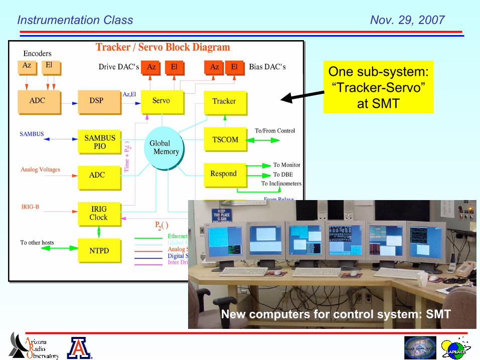
One sub-system:“Tracker-Servo”

at SMT

New computers for control system: SMT


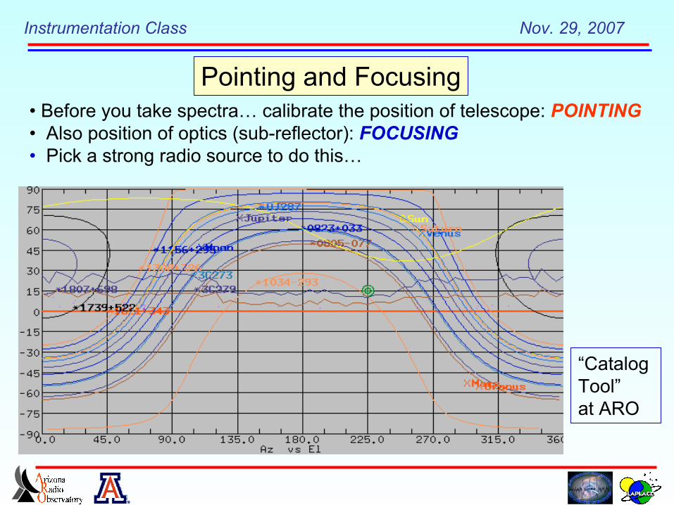
• Before you take spectra… calibrate the position of telescope: POINTING• Also position of optics (sub-reflector): FOCUSING• Pick a strong radio source to do this…

Pointing and Focusing

“CatalogTool”at ARO


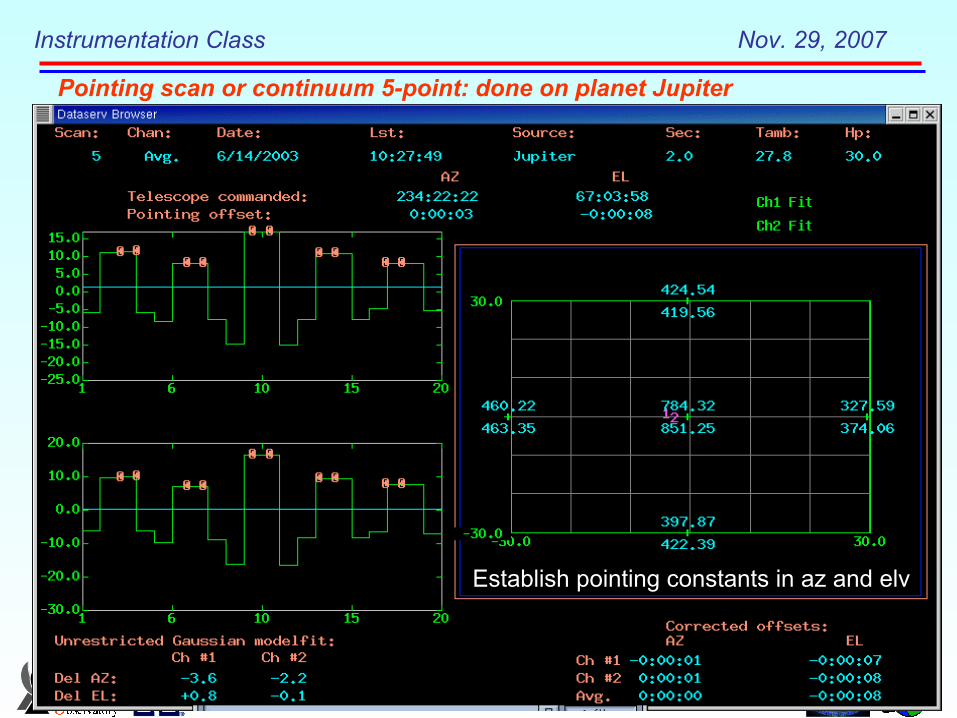
Pointing scan or continuum 5-point: done on planet Jupiter

Establish pointing constants in az and elv


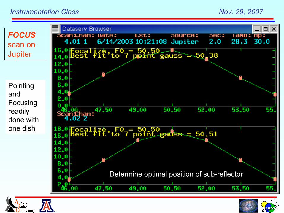
FOCUSscan onJupiter

Determine optimal position of sub-reflector

PointingandFocusingreadilydone withone dish


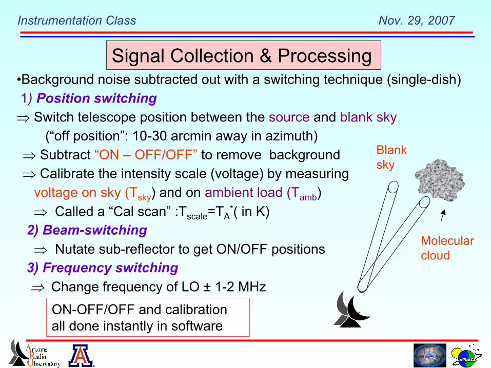
•Background noise subtracted out with a switching technique (single-dish) 1) Position switching⇒ Switch telescope position between the source and blank sky (“off position”: 10-30 arcmin away in azimuth)⇒ Subtract “ON – OFF/OFF” to remove background⇒ Calibrate the intensity scale (voltage) by measuring voltage on sky (Tsky) and on ambient load (Tamb) ⇒ Called a “Cal scan” :Tscale=TA

*( in K) 2) Beam-switching ⇒ Nutate sub-reflector to get ON/OFF positions 3) Frequency switching ⇒ Change frequency of LO ± 1-2 MHz

Signal Collection & Processing

Molecularcloud

Blanksky

ON-OFF/OFF and calibrationall done instantly in software


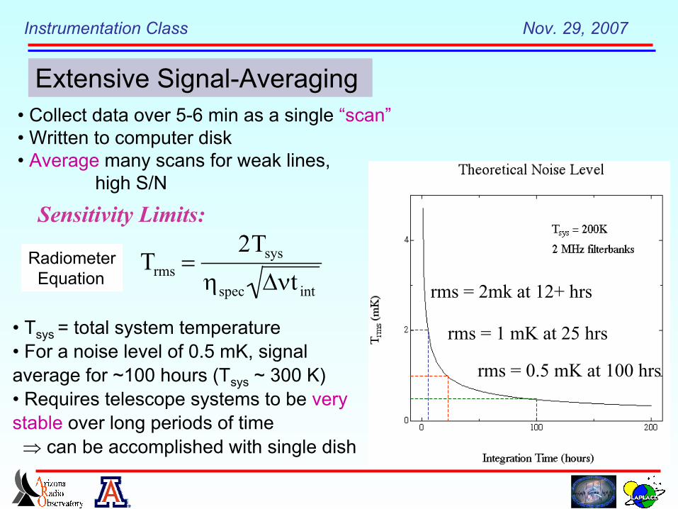
Sensitivity Limits:

Trms =2Tsys

ηspec ∆νt int

• Tsys = total system temperature• For a noise level of 0.5 mK, signalaverage for ~100 hours (Tsys ~ 300 K)• Requires telescope systems to be verystable over long periods of time ⇒ can be accomplished with single dish

rms = 2mk at 12+ hrs

rms = 1 mK at 25 hrs

rms = 0.5 mK at 100 hrs

Extensive Signal-Averaging • Collect data over 5-6 min as a single “scan”• Written to computer disk• Average many scans for weak lines, high S/N

Radiometer Equation


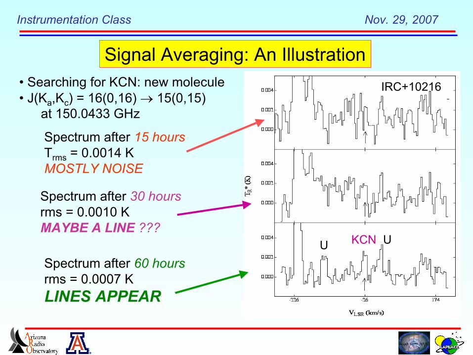
Spectrum after 15 hoursTrms = 0.0014 KMOSTLY NOISE

Spectrum after 30 hoursrms = 0.0010 KMAYBE A LINE ???

Spectrum after 60 hoursrms = 0.0007 KLINES APPEAR

• Searching for KCN: new molecule• J(Ka,Kc) = 16(0,16) → 15(0,15) at 150.0433 GHz

Signal Averaging: An IllustrationIRC+10216

KCN UU


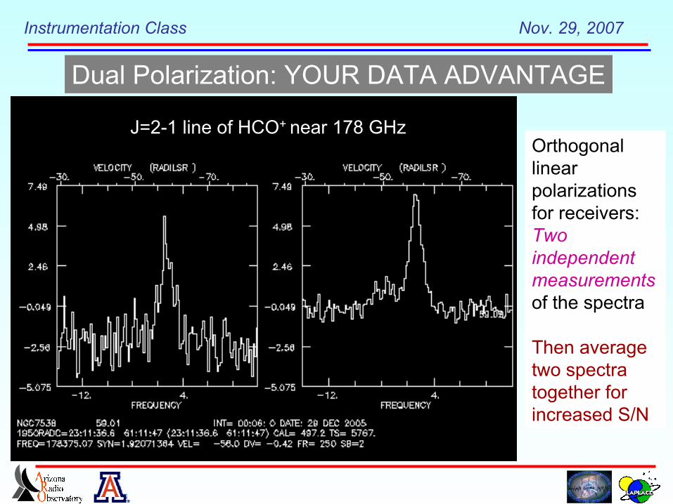
Dual Polarization: YOUR DATA ADVANTAGE

J=2-1 line of HCO+ near 178 GHzOrthogonallinearpolarizationsfor receivers:Twoindependentmeasurementsof the spectra

Then averagetwo spectratogether forincreased S/N


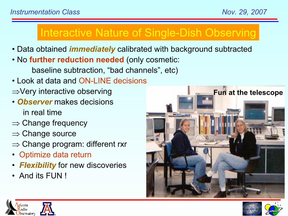
• Data obtained immediately calibrated with background subtracted• No further reduction needed (only cosmetic: baseline subtraction, “bad channels”, etc)• Look at data and ON-LINE decisions⇒Very interactive observing• Observer makes decisions in real time⇒ Change frequency⇒ Change source⇒ Change program: different rxr• Optimize data return• Flexibility for new discoveries • And its FUN !

Interactive Nature of Single-Dish Observing

Fun at the telescope


0.6

0.4

0.2

0.0

T R* (K

)

226800226600226400Frequency (MHz)

J = 1.5 - 1.5hf components



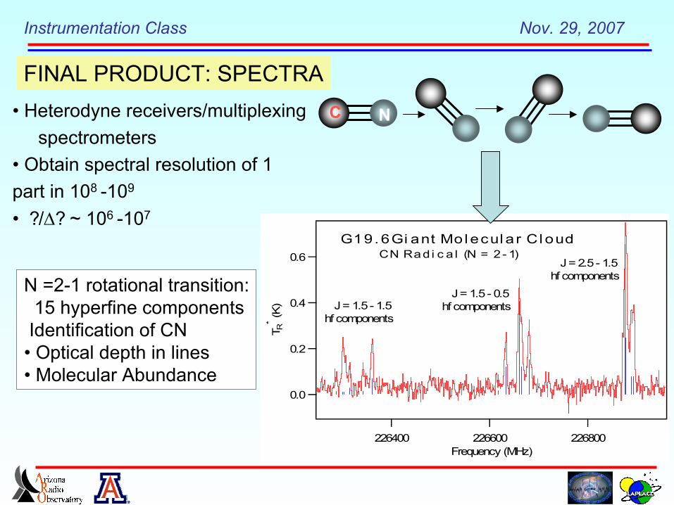
G 1 9 . 6 G i a n t M o l e c u l a r C l o u d C N R a d i c a l (N = 2 - 1)

C N

N =2-1 rotational transition: 15 hyperfine components Identification of CN• Optical depth in lines• Molecular Abundance

FINAL PRODUCT: SPECTRA• Heterodyne receivers/multiplexing spectrometers • Obtain spectral resolution of 1part in 108 -109

• ?/∆? ~ 106 -107


1.4

1.2

1.0

0.8

0.6

0.4

0.2

0.0

T R* (K

)

232000231800231600231400231200231000Frequency (MHz)

13C

S

OC

S

C2H

3CN

C2H

3CN

C2H

3CN

CH

3CH

O +

C2H

3CN

CH

3CH

O +

C2H

5CN

C2H

3CN

C2H

3CN

HC

OO

CH

3 + C

2H3C

N

C

2H3C

N

C2H

5CN

C2H

5CN

C2H

5CN

C2H

5CN

HC

OO

CH

3

HC

OO

CH

3

HC

OO

CH

3

HC

OO

CH

3

HC

OO

CH

3

CH

3CH

O

C2H

3CN

+ C

2H5C

N

C2H

5OH

C2H

5OH

+ (C

H2O

H) 2

CH

3CH

O

C2H

5OH

CH

3NH

2

HN

CO

CH

3CH

O

CH

3CH

O

HC

OO

H

C2H

5OH

(CH

3)2O

(CH

3)2O

NH

2CH

O

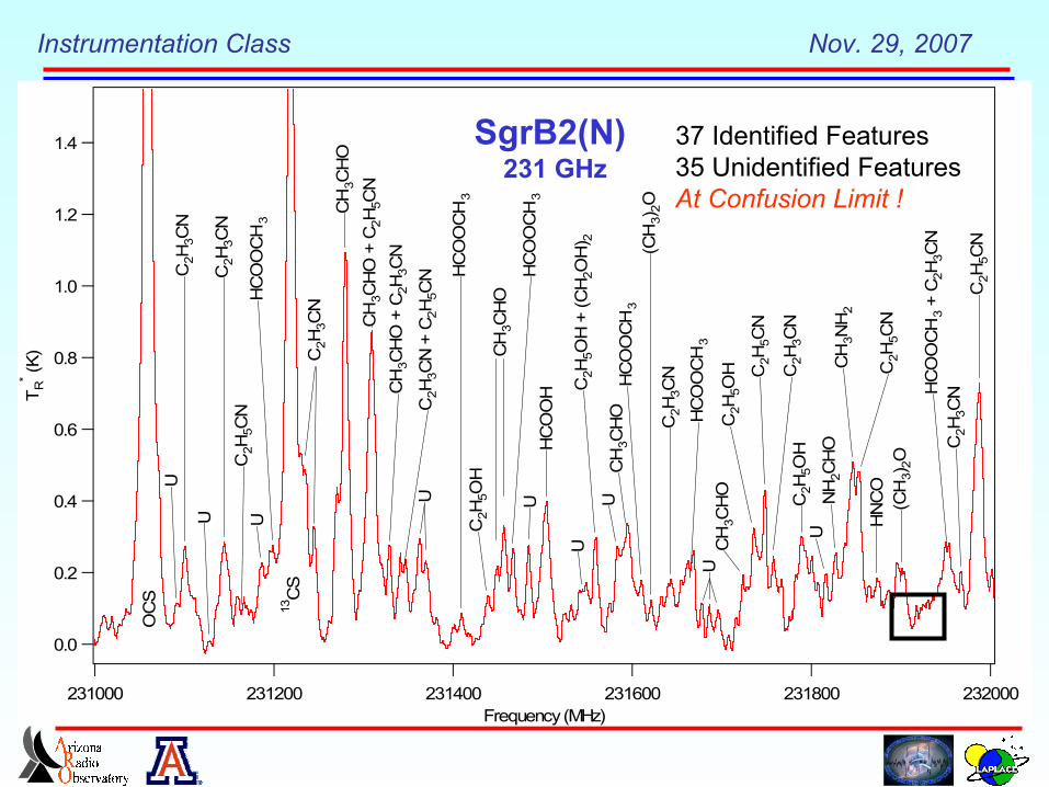
37 Indentified Features35 Unidentified Features~6 lines per 100 km/sTRMS = 0.003 K (theoretical)

U

U U

U U

U

U

U

U

37 Identified Features35 Unidentified FeaturesAt Confusion Limit !

SgrB2(N) 231 GHz


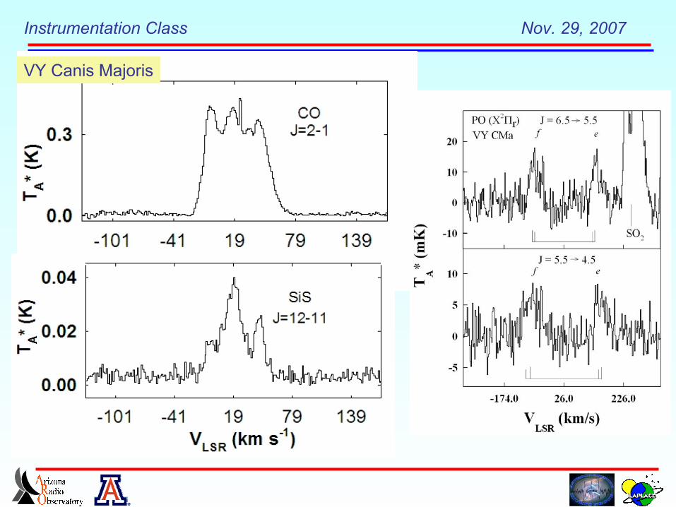
VY Canis Majoris


. ........

.....

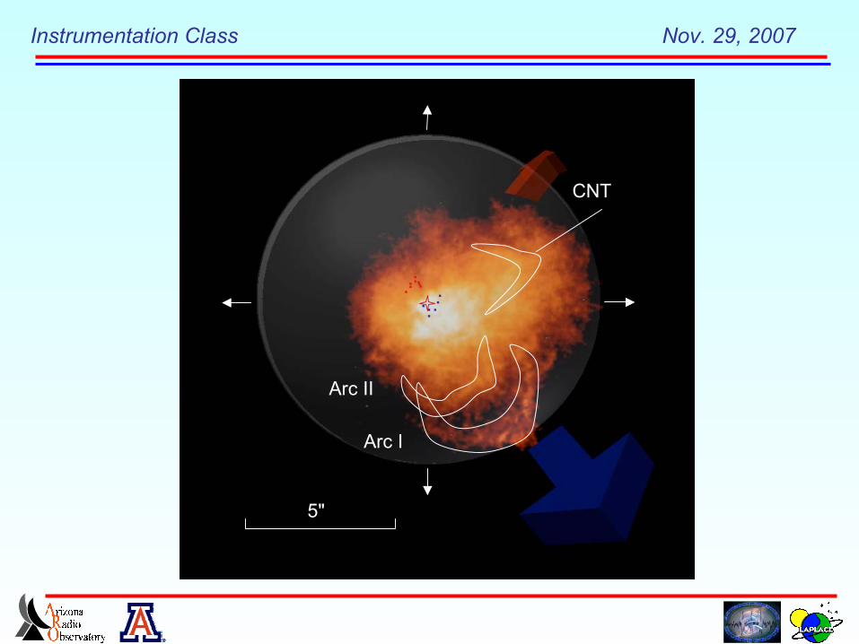
5"

Arc I

Arc II

CNT


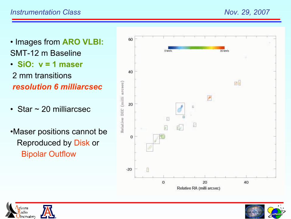
• Images from ARO VLBI:SMT-12 m Baseline• SiO: v = 1 maser 2 mm transitions resolution 6 milliarcsec

• Star ~ 20 milliarcsec

•Maser positions cannot be Reproduced by Disk or Bipolar Outflow

Documents

Radio Telescopes and Interferometry