RADIATED UNDERWATER NOISE MEASURED FROM THE

DRILLING RIG OCEAN GENERAL, RIG TENDERS

PACIFIC ARIKI AND PACIFIC FRONTIER, FISHING VESSEL

REEF VENTURE AND NATURAL SOURCES

IN THE TIMOR SEA, NORTHERN AUSTRALIA

Prepared for:

Shell AustraliaShell House Melbourne

By:

Rob McCauley

July 1998

PROJECT CMSTREPORT C98-20

CENTRE FOR MARINE SCIENCE AND TECHNOLOGYCURTIN UNIVERSITY OF TECHNOLOGYWESTERN AUSTRALIA 6102

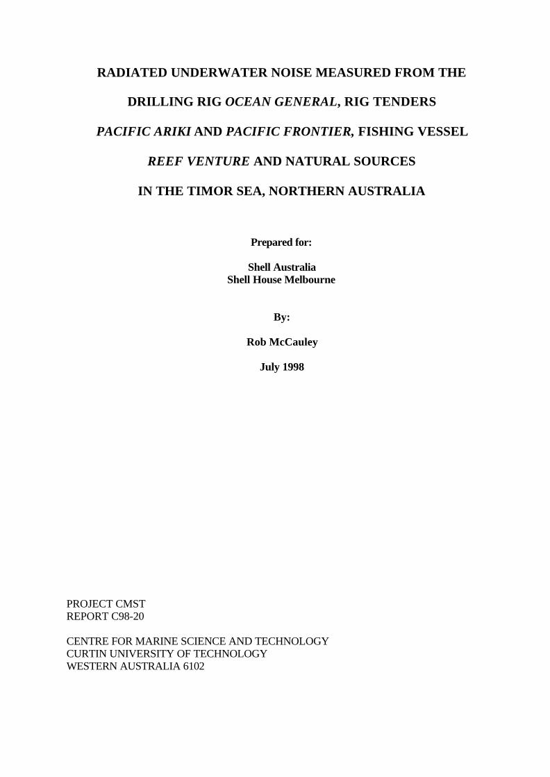
Figure 1 Photograph of the exploratory drilling rig Ocean General with the rig tender Pacific Frontier standing by (looking from north, off aft port quarter).

i

ABSTRACT

Between the 21st and 23rd March 1998 measurements were made of the radiated underwater noisefrom the exploration drilling rig Ocean General, the rig tenders Pacific Ariki and Pacific Frontiermaintaining position at the rig for supply purposes, the Pacific Ariki steaming at 11 knots and thefishing vessel Reef Venture steaming at 12 knots. Measurements were also taken of the local ambientnoise with no vessel or rig noise input. The study region was 160 km NNW of the northern tip ofMelville Island in the Timor Sea, in 110 m water depth 13 km inside the shelf edge 200 m depthcontour.

Over the study period the Ocean General was involved in coring work, maintenance of the drill holeand active drilling, with the well head at 3,600-3,700 m. The rig was moored on eight anchors and hadno active positioning systems. The major items of machinery aboard the rig were located on decks wellabove the waterline. The Pacific Ariki and Pacific Frontier were similar vessels, 64 m length, 5 mdraught displacing around 2600 tonnes depending on load, with four main engines totalling 8000 Hpdriving through two shafts with fully feathering propellers, and having through-hull, transverse bow-thrusters. The Reef Venture was 20 m length, displaced 20-30 tonnes and had a single main engine of450 Hp.

Conditions were almost dead calm during the study period thus there was little masking of vesselsignatures by wind or sea noise. A broadband ambient level of 90 dB re 1µPa was recorded, this isbelieved to be close to the lowest level possible in the region. Fish choruses were recorded from Shoals8 km to the north and south of the Ocean General on all evenings sampled. It is believed the signatureof these choruses was also evident from immediately astern the Ocean General. Dolphins were heardin many recordings from short and long range from the rig.

The noise produced by the drilling rig emanated from three sources. The quietest period was the rigworking but not drilling with the tender on anchor. During this period the primary noise sources werefrom mechanical plant, discharged fluids, pumping systems and miscellaneous banging of gear on the rig.As the main machinery deck of the rig was well above the waterline the overall noise level was low, thenear field corresponded roughly to the rig dimensions, and the highest broadband level encountered was117 dB re 1µPa at 125 m from the wellhead. Various tones produced by machinery can be seen in thespectra of this noise. Under this operating condition and the calm sea conditions encountered, the rignoise was audible for 1-2 km.

The second noise source involved the rig actively drilling and the rig tender on anchor. The drill stringproduced dominant tones, notably in the 31 and 62 Hz 1/3 octaves. The drill string was considered tobe a vertical line source some 3.8 km long comprising a steel tube (drill string) rotating in a steel (inwater) or concrete (subsea) casing. Thus two sources were active, the rig itself and the drill string. Asharp near-far field transition was observed at around 400 m. While drilling and at ranges of less than400 m from the wellhead the drill-rig noise dominated, so that measurements matched those of periodswhen the rig was not drilling. Beyond 400 m significant energy from the drill string tones becameapparent resulting in an increase in the received noise level. For the rig drilling, the highest noise levelsencountered were of the order 115-117 dB re 1µPa at 405 and 125 m respectively, with the rigaudible out to 11 km.

The third noise source, which far exceeded the previous two, involved a rig tender standing by the rigfor loading purposes. The tenders stood off the port or starboard side on a bow anchor, kept the mainshafts spinning with the propellers feathered, and applied pitch to the propellers and activated the bowthrusters as required. Strong currents were experienced in the region, these caused the skippers to

ii

almost continually apply bow and main shaft thrust to stop the vessel laying off. The use of the thrustersor main propellers under load produced very high levels of cavitation noise. This noise was broadbandin nature, with the highest level measured at 137 dB re 1µPa at 405 m astern the rig, levels of 120 dBre 1µPa recorded at 3-4 km and the noise audible at up to 20 km.

The noise of the Pacific Ariki and the Reef Venture underway was audible out to about 10 and 5.5km from each vessel respectively, with the 120 dB re 1µPa contour at 0.5-1 km for the Pacific Arikiand 250 m for the Reef Venture. Each vessel produced a complex mix of machinery and cavitationnoise.

Vertically separated and drifting hydrophones, set over the study period, revealed that there werestrong differential currents throughout the water column. Temperature, salinity and depth castssuggested that a deep body of colder water may have been creeping up the shelf whilst warmer waterflowed over the top, setting in a general NW direction with a local tidal flow superimposed.

ACKNOWLEDGMENTS

This work has been funded and supported by Shell Australia (Shell House, 1 Spring St. Melbourne,Vic 3000). Roel Kleijn and Wim Adolfs of Shell were instrumental in defining the projects scope andensuring the work proceeded smoothly. The seamanship skills of Curt Jenner (Centre for WhaleResearch Western Australia, Inc.) were essential in the success of the field trials. Alec Duncan and LesDenison of the Centre for Marine Science and technology assisted in gear preparation, Alec alsoprovided valuable comments on this document. The Reef Venture crew Jamie Perry (skipper), thedeckhands, and the vessels owner, Clive Perry, did everything possible to ensure field trials ransmoothly. The crews of the Pacific Ariki, Pacific Frontier and the Ocean General always respondedimmediately to our many requests for information and provided invaluable information on the operationsof their respective vessels. The Pacific Ariki crew were particularly helpful in the conduct of a pass bya drifting housing.

iii

CONTENTS

ABSTRACT.......................................................................................................................................i

ACKNOWLEDGMENTS ................................................................................................................ ii

CONTENTS.................................................................................................................................... iii

DEMONSTRATION TAPE............................................................................................................ iv

1) INTRODUCTION........................................................................................................................5

2) METHODS...................................................................................................................................62.1) Field work / site / environmental conditions......................................................................62.2) Equipment ....................................................................................................................10

2.2.1) Acoustic equipment........................................................................................102.2.2) GPS / CTD profiler / Echosounder logs..........................................................12

2.3) Analysis........................................................................................................................142.3.1) Acoustic analysis............................................................................................142.3.2) Position .........................................................................................................15

2.4) Vessel specifications and activities.................................................................................152.4.1) Ocean General...............................................................................................152.4.2) Pacific Ariki & Pacific Frontier.......................................................................152.4.3) Reef Venture & Nova....................................................................................16

3) RESULTS / DISCUSSION ........................................................................................................163.1) Ambient noise...............................................................................................................16

3.1.1) Lowest ambient measured..............................................................................163.1.2) Biological sea-noise sources...........................................................................18

3.2) Rig (Ocean General) noise ............................................................................................223.2.1) Ocean General and tender on station noise character.....................................22Drilling noise, tender on anchor.................................................................................243.2.2) Rig noise with range .......................................................................................27

3.3) Vessel noise..................................................................................................................323.3.1) Propagation...................................................................................................323.3.2) Pacific Ariki and Reef Venture noise patterns ...............................................35

3.4) Hydrophone flow noise, CTD Casts and hydrographic regime........................................41

4) GENERAL DISCUSSION.........................................................................................................46

REFERENCES ...............................................................................................................................49

APPENDIX 1:.................................................................................................................................51

Appendix 2:.....................................................................................................................................52

iv

DEMONSTRATION TAPE

Item

1) Low background sea noise measured over study period (no vessel noiseinput, from open water, 25 m hydrophone depth)

2) Fish chorus as heard on the southern side Tasmania Shoal

3) Dolphins recorded near the Ocean General

4) Ocean General working but not drilling with the rig tender on anchor(from bottomed hydrophone 450 m astern rig)

5) Ocean General drilling with rig tender on anchor (from bottomedhydrophone 450 m astern the rig)

6) Rig tender holding station off the Ocean General (from bottomedhydrophone 450 m astern the rig)

7) Pacific Ariki at 400-500 m passing hydrophone at 25 m depth

8) Reef Venture passing hydrophone at 25 m depth with closestapproach 30 m

9) Reef Venture manoeuvring over top of hydrophone at 25 m depth

10) Zodiac dinghy manoeuvring over top hydrophone at 25 m depth

5

1) INTRODUCTIONOver the period 20th-24th March 1998 the Centre for Marine Science and Technology conducted field workin the vicinity of the oil drilling rig, Ocean General located in the Timor Sea, to measure the radiatedunderwater noise of the drilling rig and its associated supply vessels. The program objectives for thesemeasurements were:

1) Using calibrated systems, quantify underwater noise source-levels of active drill ship and selection ofservice vessels working permit NT/P48;

2) Measure reduction of drill ship noise with increasing range at several water depths;

3) Measure noise levels of drill ship at Evans Shoal and surrounding bank and un-named shoalapproximately 5 nautical miles south of drilling operations;

4) Measure ambient sea-noise at time of sampling from nearby shoal with no rig-noise;

5) As best as possible describe sound propagation at the site;

6) Use noise levels of drill operations, sound propagation and influence of ambient sea-noise to predictnoise levels of drilling operations experienced at increasing range from drill rig.

7) Use noise levels produced by drilling operations and available literature on effects of noise on fin-fish topredict possible effects of drilling noise on nearby fisheries operations.

8) Measure biological sea-noise at the site and determine if this is different than expected or possiblyinfluenced by drilling operations noise.

The complete program of work also includes modelling the horizontal propagation of seismic-survey air-gunsignals in the region of permit NT/P48. This modelling program is to be carried out separately to theunderwater drill noise and vessel noise measurements.

The work described here has been carried out as an extension of the Centre for Marine Science andTechnology's current APPEA/ERDC project which is studying the effects of seismic survey noise on marineanimals.

This document presents an analysis of the Timor Sea underwater noise measurements and synthesises theseresults with respect to possible biological effects. For clarity in interpretation the discussion of the noisemeasurements is included with the results. The final discussion considers the biological implications of the noiseproduced by the Ocean General and rig-tender operations.

To clarify the types and comparative levels of noise described a demonstration tape is included with thereport. Where applicable this tape is indexed into the report.

6

2) METHODS

2.1) Field work / site / environmental conditionsThe exploration drilling rig Ocean General (OG) was moored with eight anchors 160 km (85 nautical mile)NNW of the northern tip of Melville Island in 110 m water depth. Vessel details are given in section 2.4. Co-ordinates of the well-head were: 10o 2.1' S, 129o 33.5' E. Water depths were relatively uniform in the vicinityof the rig with a general flat bottom. Evans Shoal lay eight km north of the rig and an un-named shoal referredto as Tasmania Shoal by the local fisherman, lay nine km to the south. The northern edge of the continentalshelf (200 m depth contour) lay some 15 km north of the rig's position. Numerous shoals and reefs lay justinside the 200 m contour, extending west of the OG's position.

Over the 21st to 24th March 1998 the vessel Reef Venture (RV) was chartered to conduct underwater noisemeasurements around the OG. Approximately 560 recordings ranging from 51 s to 4 hours were made in thevicinity of the OG. Recordings were made from a 4 m inflatable dinghy (Nova), from bottom mooredautonomously operating packages (two of), a drifting package set to operate in free run mode, and a mooredmid water package operating autonomously. Recordings were made at ranges of from 125 m to 22.5 km fromthe OG.

Locations of the general area, recording sites and CTD cast-positions are shown on Figure 2, Figure 3 andFigure 4 at decreasing scales. These figures are referred to the well head position (zero point) using themethod described in section 2.3.2.

Full details of field activities made over the three days on site are listed in Appendix 1.

Weather over the study period was extremely calm. The highest winds experienced aboard the RV were lessthan 10 knots, with 'average' wind speeds of less than 5 knots. Sea conditions were thus calm throughout witha low swell.

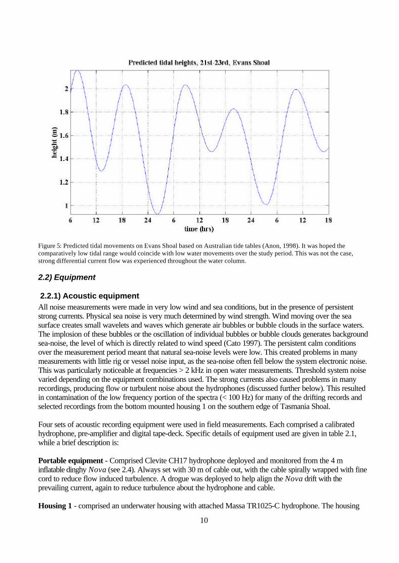
The Australian Tide Tables (Anon, 1998) shows Evans Shoal as having diurnal tides, and lists tidalcharacteristics using Darwin harbour as a primary port. Using the simple tidal predictions given in Anon(1998) the predicted tidal regime over the study period for Evans Shoal is shown on Figure 5. A time of neaptides (predicted maximum tidal range of 1 m) was chosen for the field measurements so as to reduce thechance of encountering strong tidal flows. Flow induced turbulence around any suspended hydrophone andassociated cable moored in a current produces pressure fluctuations at the hydrophone. This translates toartificially high measurements of noise, generally at frequencies below 100 Hz. By timing the field work to takeplace at neap tides it was hoped to largely avoid this artificial noise. As it transpired, over the study period apersistent and strong surface current setting mostly to the NW with sub-surface currents believed to betravelling at different rates and / or in different directions were experienced. Severe problems wereexperienced with flow / turbulent noise in some hydrophone sets, particularly drifting sets where twohydrophones vertically separated by 50 m were deployed. Differential flow across the 50 m of cable renderedthe lower hydrophone recordings in these sets useless for sea-noise work at frequencies below about 150 Hzbecause of cable and hydrophone flutter. They did provide interesting information on the hydrographic regimeof the area though. This is discussed in section 3.3.

7

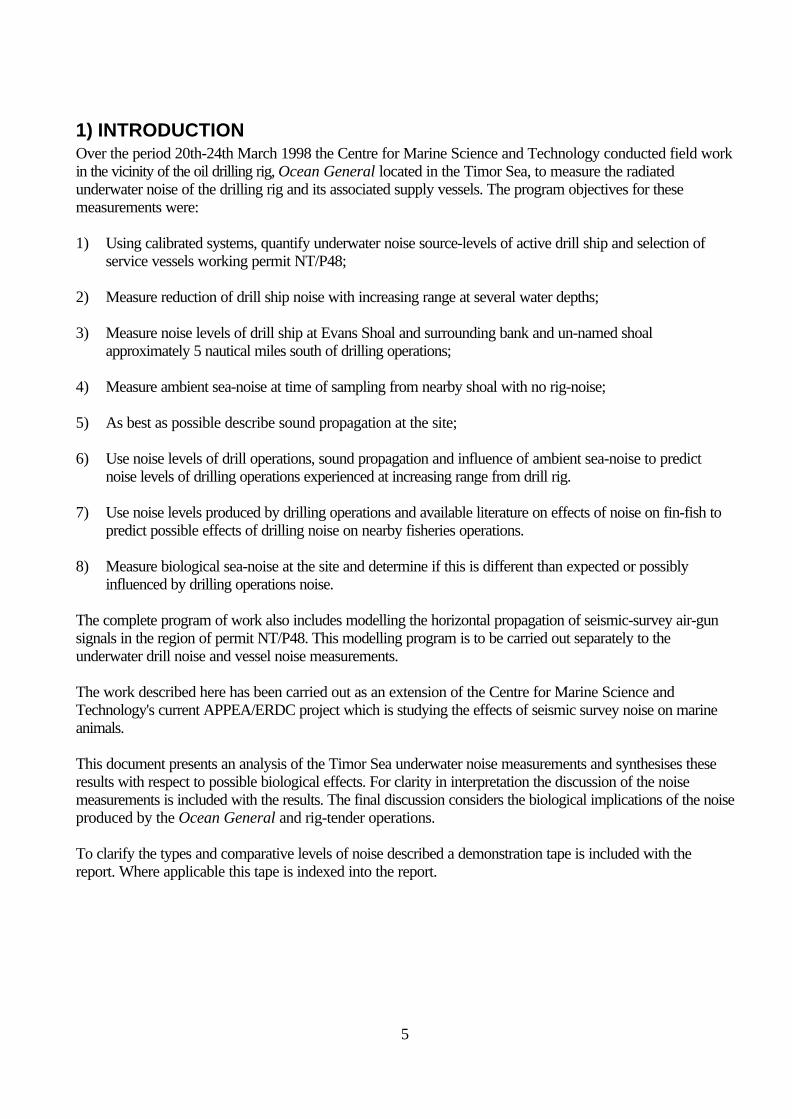
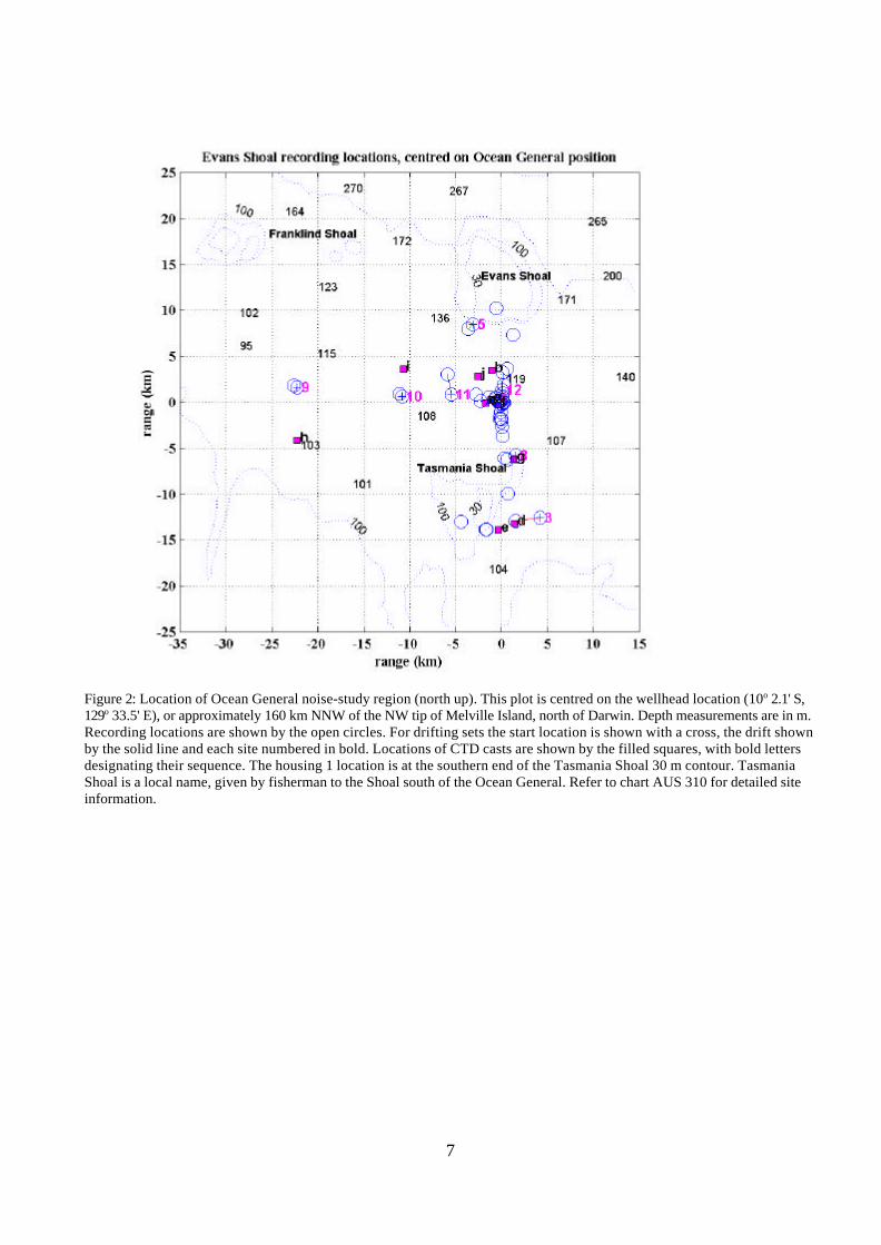
Figure 2: Location of Ocean General noise-study region (north up). This plot is centred on the wellhead location (10o 2.1' S,129o 33.5' E), or approximately 160 km NNW of the NW tip of Melville Island, north of Darwin. Depth measurements are in m.Recording locations are shown by the open circles. For drifting sets the start location is shown with a cross, the drift shownby the solid line and each site numbered in bold. Locations of CTD casts are shown by the filled squares, with bold lettersdesignating their sequence. The housing 1 location is at the southern end of the Tasmania Shoal 30 m contour. TasmaniaShoal is a local name, given by fisherman to the Shoal south of the Ocean General. Refer to chart AUS 310 for detailed siteinformation.

8

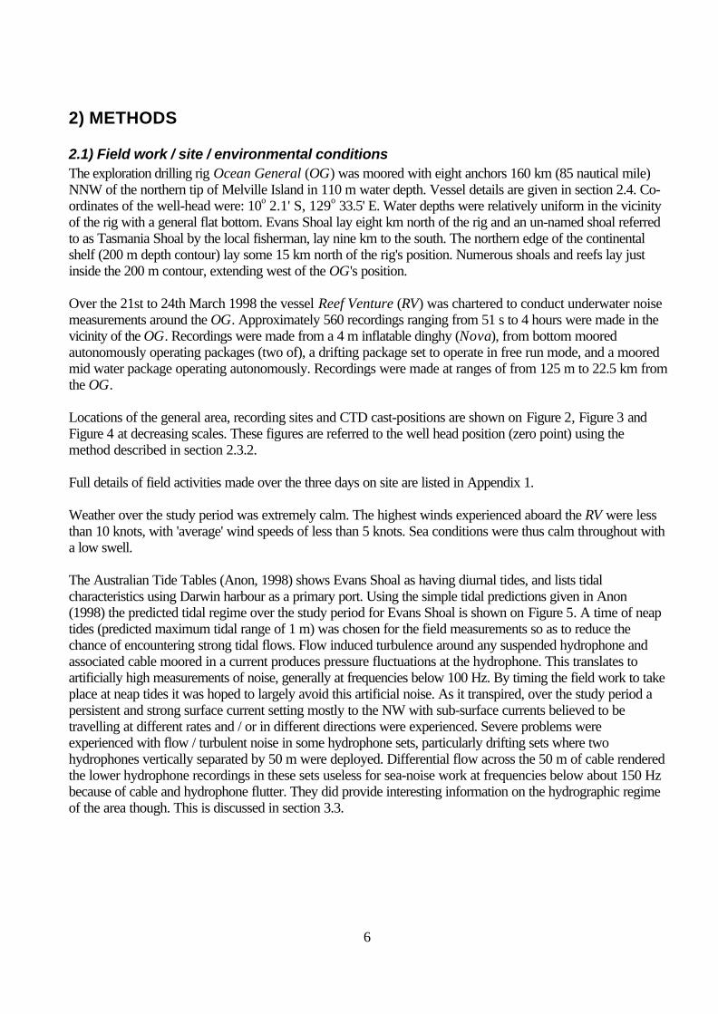
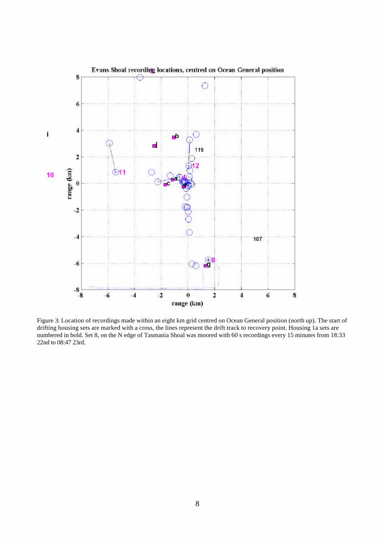
Figure 3: Location of recordings made within an eight km grid centred on Ocean General position (north up). The start ofdrifting housing sets are marked with a cross, the lines represent the drift track to recovery point. Housing 1a sets arenumbered in bold. Set 8, on the N edge of Tasmania Shoal was moored with 60 s recordings every 15 minutes from 18:3322nd to 08:47 23rd.

9

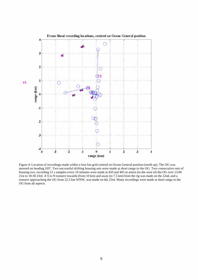
Figure 4: Location of recordings made within a four km grid centred on Ocean General position (north up). The OG wasmoored on heading 105o. Two successful drifting housing sets were made at short range to the OG. Two consecutive sets ofhousing two, recording 51 s samples every 10 minutes were made at 450 and 405 m astern (to the west of) the OG over 13:0021st to 18:30 23rd. A S to N transect towards (from 10 km) and away (to 7.5 km) from the rig was made on the 22nd, and atransect approaching the OG from 22.5 km WNW, was made on the 23rd. Many recordings were made at short range to theOG from all aspects.

10

Figure 5: Predicted tidal movements on Evans Shoal based on Australian tide tables (Anon, 1998). It was hoped thecomparatively low tidal range would coincide with low water movements over the study period. This was not the case,strong differential current flow was experienced throughout the water column.

2.2) Equipment

2.2.1) Acoustic equipmentAll noise measurements were made in very low wind and sea conditions, but in the presence of persistentstrong currents. Physical sea noise is very much determined by wind strength. Wind moving over the seasurface creates small wavelets and waves which generate air bubbles or bubble clouds in the surface waters.The implosion of these bubbles or the oscillation of individual bubbles or bubble clouds generates backgroundsea-noise, the level of which is directly related to wind speed (Cato 1997). The persistent calm conditionsover the measurement period meant that natural sea-noise levels were low. This created problems in manymeasurements with little rig or vessel noise input, as the sea-noise often fell below the system electronic noise.This was particularly noticeable at frequencies > 2 kHz in open water measurements. Threshold system noisevaried depending on the equipment combinations used. The strong currents also caused problems in manyrecordings, producing flow or turbulent noise about the hydrophones (discussed further below). This resultedin contamination of the low frequency portion of the spectra (< 100 Hz) for many of the drifting records andselected recordings from the bottom mounted housing 1 on the southern edge of Tasmania Shoal.

Four sets of acoustic recording equipment were used in field measurements. Each comprised a calibratedhydrophone, pre-amplifier and digital tape-deck. Specific details of equipment used are given in table 2.1,while a brief description is:

Portable equipment - Comprised Clevite CH17 hydrophone deployed and monitored from the 4 minflatable dinghy Nova (see 2.4). Always set with 30 m of cable out, with the cable spirally wrapped with finecord to reduce flow induced turbulence. A drogue was deployed to help align the Nova drift with theprevailing current, again to reduce turbulence about the hydrophone and cable.

Housing 1 - comprised an underwater housing with attached Massa TR1025-C hydrophone. The housing

11

was moored in 70 m of water at the southern edge of the shallow section of Tasmania Shoal, so as to beshielded from any noise produced by the OG and supply vessels working in its vicinity. The housing andhydrophone were set on the bottom. The unit operated on a timing cycle of a 3 minute recording every 45minutes from 11:30 on the 21st to 19:30 on the 23rd. Unfortunately this housing was set with 250 m of 16 mmline with ~ 100 m of the line coiled in a bundle at the surface. The strong persistent currents experienced at thesite combined with the drag of the bundled line produced large, persistent flutter in the mooring line and somemovement of the housing. This produced artificial pressure fluctuations at the hydrophone, making manyrecordings below ~ 150 Hz of limited value.

Housing 2 - Comprising an underwater housing with an attached Brüel & Kjær hydrophone, operating on atiming cycle of a 51 s recording every 10 minutes. The hydrophone signal was split and recorded with differentgains to separate channels of the tape deck. Two consecutive deployments were made at 420 m and 405 mastern of (or to the west of) the OG in 113 m of water. In both sets the housing and hydrophone lay on thebottom. A full 250 m coil of 16 mm line led to surface buoys and floats. No flow noise problems wereexperienced with either deployment.

Housing 1A - Comprised an underwater housing with two GEC-Marconi SH101-X hydrophones attached.This housing was normally drifted with the tape deck continuously recording. The housing was set at 30 mdepth with 16 mm line attached to surface buoys and floats. One hydrophone was buoyed 5 m above thehousing (25 m depth) with the deployment configuration such that the buoyed hydrophone did not foul thesurface line, while the second hydrophone hung 45 m below the housing (75 m depth). A depth gaugerecorded the maximum housing depth reached in each deployment. Each hydrophone recorded throughindividual pre-amplifiers, to separate channels of the tape deck. One overnight deployment was made with thehousing and hydrophones set as above, but the surface floats attached to a mooring. In this set the unitoperated on a timing cycle of a 60 s recording every 15 minutes. The shallow and deep hydrophones were thesame in each set, but they were regularly swapped through the amplifier-tape-deck combination.

The drifting sets were made in the belief that the entire unit would drift with any prevailing current or tidalstream, so minimising flow noise. This was not the case. In all six successful drifting sets (in one set the tapedeck failed), the bottom hydrophone recorded high levels of low frequency noise while the top hydrophonerecorded much lower levels.

Equipment failure or some real effect were ruled out as possible causes of this noise. No equipment checkswith any combinations of equipment before or after field trials revealed any faults, and swapping thehydrophone-amplifier-tape-channel combinations during field trials did not change the results. The levels oflow frequency noise recorded by the bottom hydrophone of this housing were consistently high at all sites, farabove measurements made at similar sites and times from shallower hydrophones (including the housing's 25m hydrophone and separate recording packages), and greater than any recorded by the bottom mountedpackage immediately astern the OG. Although a downward refracting sound speed gradient was observed, itis inconceivable that the high levels of low frequency noise would not have been heard in the shallowrecordings. Thus this low frequency noise is believed to be the result of the bottom hydrophone being draggedat a different rate and probable direction to the housing and top hydrophone. This would have set up strongfluttering of the bottom hydrophone cable, so producing high levels of turbulence about the hydrophone.

Time basesAll tape decks maintained and wrote to tape a time base. The time bases of a master watch and each tapedeck were regularly checked against the displayed GPS time. Central Standard Time was maintained on alltime-pieces. Deployment and recovery time and position of each hydrophone set was logged. Using the timebases written to the tapes and GPS or drilling logs, enabled calculations of ranges from drilling rig or vessel asappropriate, or correlations of measured noise with drilling activities.

12

CalibrationsAll hydrophones were supplied with factory calibrations sheets for sensitivity. The sensitivity of the Brüel &Kjær 8104 hydrophone used in the housing 2 sets (immediately astern the OG) was calibrated with a Brüel &Kjær type 4223 hydrophone calibrator, and found to be within 0.9 dB of the factory calibration specificationsat the pre-set tones of 250 and 320 Hz used by the unit. The sensitivity of the other hydrophones was thenchecked against the Brüel & Kjær hydrophone.

The frequency response of each hydrophone-pre-amplifier-tape deck combination was determined bycharacteristics of each component, specifically the pre-amplifier and hydrophone capacitance, the in builttape-deck roll off at low and high frequencies and the hydrophone response. To check the response of eachcombination in the field, white or pink noise of known level was recorded for each tape-deck-pre-amplifiercombination before each set of recordings. White-noise is random noise of statistically equal intensity at allfrequencies, while pink-noise is noise of decreasing intensity at increasing frequency such that 1/3 octaveanalysis (or analysis in steps of geometrically increasing bandwidths) gives equal measures across thefrequency spectra. These calibrations were later compared with white and pink noise measurements madewith the appropriate hydrophone in series with the pre-amplifier and tape deck combinations. Using thehydrophone in series will give a better description of the appropriate combination of equipment's lowfrequency roll-off. From the calibrations with the hydrophone in series, and the known sensitivity of eachhydrophone, calibration curves for each set of equipment were derived. These are shown in Figure 6 for 1/3octave measurements. By comparing these curves with calibration curves recorded during the field and asanalysed, composite calibration curves were applied as appropriate to each analysis set.

2.2.2) GPS / CTD profiler / Echosounder logsPosition fixing was by: 1) aboard the RV, differential GPS system comprising Fugro differential unit using aGarmin 45 GPS and output to two laptop computers; 2) GPS positions manually read from the RV navigationsystem which comprised a Furuno GP 70 MkII GPS interfaced to a Furuno FR 8100-D 48 mile radar and aFuruno GD-188 plotter; 3) in Nova at > 350 m from the OG, a Garmin 38 hand held GPS; or 4) in Novaand at < 350 m from the OG, bearing from hand bearing compass and range from Bushnell laser range findingbinoculars. Despite almost ideal conditions and a good sighting target (the OG legs, shipping containers or hutson deck), the Bushnell binoculars could only locate the OG at < 350 m. Laser range sightings off the OG werereduced to ranges from the wellhead using the OG deck plans. The RV differential GPS position wascontinuously logged to computer at a 2 s output rate. The Furuno and Garmin 38 readings were manually readoff the GPS or radar unit.

A system for logging echosounder returns was installed in parallel with the ships Furuno 292 echosoundertransducer. The 50 kHz transducer outgoing and returning pulses were continuously monitored by theEchoListener system (SonarData Tasmania Pty. Ltd.) and logged to laptop computer along with the RVdifferential GPS co-ordinates. Where required, water depths have been recovered from the stored echosounder pings.

Temperature, salinity and depth profiles were made with a Marimatech (Denmark) HMS 1820 CTD profiler.This unit was calibrated at Curtin in early March.

13

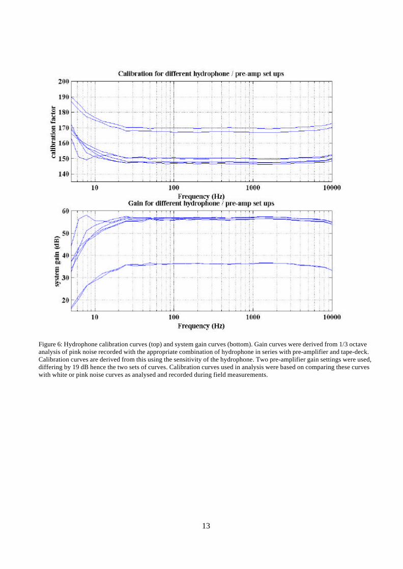
Figure 6: Hydrophone calibration curves (top) and system gain curves (bottom). Gain curves were derived from 1/3 octaveanalysis of pink noise recorded with the appropriate combination of hydrophone in series with pre-amplifier and tape-deck.Calibration curves are derived from this using the sensitivity of the hydrophone. Two pre-amplifier gain settings were used,differing by 19 dB hence the two sets of curves. Calibration curves used in analysis were based on comparing these curveswith white or pink noise curves as analysed and recorded during field measurements.

14

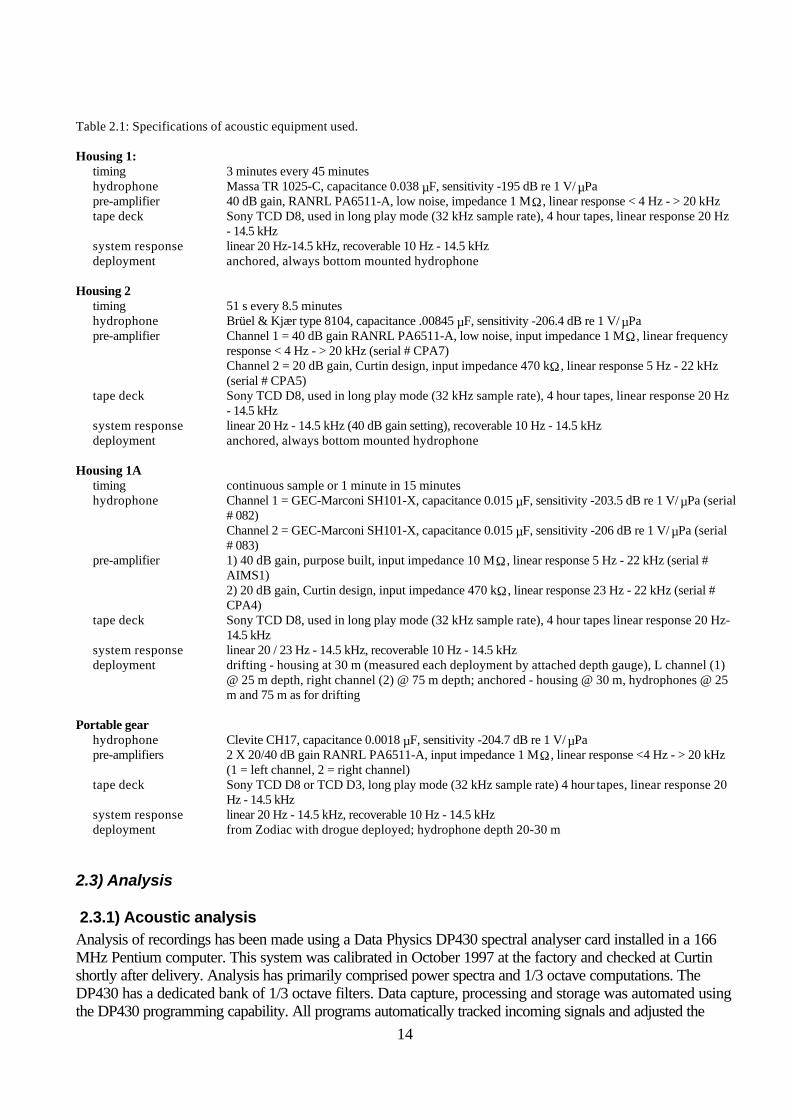
Table 2.1: Specifications of acoustic equipment used.

Housing 1:timing 3 minutes every 45 minuteshydrophone Massa TR 1025-C, capacitance 0.038 µF, sensitivity -195 dB re 1 V/ µPapre-amplifier 40 dB gain, RANRL PA6511-A, low noise, impedance 1 MΩ , linear response < 4 Hz - > 20 kHztape deck Sony TCD D8, used in long play mode (32 kHz sample rate), 4 hour tapes, linear response 20 Hz

- 14.5 kHzsystem response linear 20 Hz-14.5 kHz, recoverable 10 Hz - 14.5 kHzdeployment anchored, always bottom mounted hydrophone

Housing 2timing 51 s every 8.5 minuteshydrophone Brüel & Kjær type 8104, capacitance .00845 µF, sensitivity -206.4 dB re 1 V/ µPapre-amplifier Channel 1 = 40 dB gain RANRL PA6511-A, low noise, input impedance 1 MΩ , linear frequency

response < 4 Hz - > 20 kHz (serial # CPA7)Channel 2 = 20 dB gain, Curtin design, input impedance 470 kΩ , linear response 5 Hz - 22 kHz(serial # CPA5)

tape deck Sony TCD D8, used in long play mode (32 kHz sample rate), 4 hour tapes, linear response 20 Hz- 14.5 kHz

system response linear 20 Hz - 14.5 kHz (40 dB gain setting), recoverable 10 Hz - 14.5 kHzdeployment anchored, always bottom mounted hydrophone

Housing 1Atiming continuous sample or 1 minute in 15 minuteshydrophone Channel 1 = GEC-Marconi SH101-X, capacitance 0.015 µF, sensitivity -203.5 dB re 1 V/ µPa (serial

# 082)Channel 2 = GEC-Marconi SH101-X, capacitance 0.015 µF, sensitivity -206 dB re 1 V/ µPa (serial# 083)

pre-amplifier 1) 40 dB gain, purpose built, input impedance 10 MΩ , linear response 5 Hz - 22 kHz (serial #AIMS1)2) 20 dB gain, Curtin design, input impedance 470 kΩ , linear response 23 Hz - 22 kHz (serial #CPA4)

tape deck Sony TCD D8, used in long play mode (32 kHz sample rate), 4 hour tapes linear response 20 Hz-14.5 kHz

system response linear 20 / 23 Hz - 14.5 kHz, recoverable 10 Hz - 14.5 kHzdeployment drifting - housing at 30 m (measured each deployment by attached depth gauge), L channel (1)

@ 25 m depth, right channel (2) @ 75 m depth; anchored - housing @ 30 m, hydrophones @ 25m and 75 m as for drifting

Portable gearhydrophone Clevite CH17, capacitance 0.0018 µF, sensitivity -204.7 dB re 1 V/ µPapre-amplifiers 2 X 20/40 dB gain RANRL PA6511-A, input impedance 1 MΩ , linear response <4 Hz - > 20 kHz

(1 = left channel, 2 = right channel)tape deck Sony TCD D8 or TCD D3, long play mode (32 kHz sample rate) 4 hour tapes, linear response 20

Hz - 14.5 kHzsystem response linear 20 Hz - 14.5 kHz, recoverable 10 Hz - 14.5 kHzdeployment from Zodiac with drogue deployed; hydrophone depth 20-30 m

2.3) Analysis

2.3.1) Acoustic analysisAnalysis of recordings has been made using a Data Physics DP430 spectral analyser card installed in a 166MHz Pentium computer. This system was calibrated in October 1997 at the factory and checked at Curtinshortly after delivery. Analysis has primarily comprised power spectra and 1/3 octave computations. TheDP430 has a dedicated bank of 1/3 octave filters. Data capture, processing and storage was automated usingthe DP430 programming capability. All programs automatically tracked incoming signals and adjusted the

15

DP430 input settings to optimise the unit's dynamic range.

For long sequences of recordings (tens of minutes to hours), 5 s, 1/3 octave averages have been taken as fastas the PC would allow (every 6.4 s). For shorter samples such as those taken by housing 1 (three minsamples) and housing 2 (51 s samples) 20 s 1/3 octave averages have been mostly used. In some housing 1analysis, five or ten s averages were made, so as to avoid sections with housing movement.

The frequency content of signals is displayed either as narrow band spectra with units reduced to dB re1µPa2/Hz, or as 1/3 third octave spectra over the 1/3 octave bands of centre frequencies 10 Hz to 10 kHz(bandwidth of 9 Hz - 11.22 kHz). One-third octave analysis is most pertinent in studies of noise and its effectson animals since in all vertebrates which have been tested, 1/3 octave bands approximate the frequency spanrequired to mask narrow band signals within that frequency band. To keep with the conventions used inphysical sea noise studies and for comparison with narrow band spectral analysis, units within 1/3 octavebands are presented as dB re 1µPa2/Hz. In other studies one-third octave levels may be presented as the totalintensity within the 1/3 octave band (or in units of dB re 1µPa). To convert dB re 1µPa2/Hz to dB re 1µPaadd 10log10[bandwidth]. The 1/3 octave centre frequencies, band limits and bandwidths as used by theDP430 spectral analyser are given in appendix 2.

In some time series measures the total signal intensity within a defined bandwidth has been presented(broadband levels). These values are calculated from the sum of the 1/3 octave intensities (dB re 1µPa valuesconverted to intensity) over the specified frequency band, converted back to dB re 1µPa. Bandwidths usedwere: 1) the system limits of lower frequency 9 Hz (set by the recording hardware) to 11.22 kHz (the upperlimit of the analysers 1/3 octave analysis, 10 Hz to 10 kHz 1/3 octave bands); or 2) the 20 or 40 Hz to 10kHz 1/3 octave frequency bands (to circumvent the excessive, low-frequency flow-noise in the drifting housingsets).

2.3.2) PositionAll GPS latitude and longitude co-ordinates have been transferred to an x-y co-ordinate system usingalgorithms given by Vincenty (1975) for great circle range and bearing between two latitude and longitude co-ordinates (accurate to mm and thousandths of a degree). The zero point chosen was the well head co-ordinates for measures of the rig noise, or for vessel passbys the location of the recording hydrophone (whichhas been interpolated for drifting hydrophones).

2.4) Vessel specifications and activities

2.4.1) Ocean GeneralThe Ocean General is an exploratory drilling rig operated by Diamond Offshore. The vessel comprised twolarge submerged tubular hulls, with a network of upright legs supporting several decks of superstructure. Aphotograph of the vessel with rig tender standing by is shown in (at the documents beginning). The OG was moored using paired anchors off each quarter (eight anchors intotal), with each anchor having nearly 1.5 km of chain. The vessel was moored on heading 105o. Three dieselgenerators were used to power the rig, these were located on the main deck well above the waterline,discharging exhaust and cooling water over the port side, again above the waterline. Most other major itemsof machinery were also located on the main deck level well above the vessel's waterline.

The drilling logs of the OG were made available for correlation with measured drilling noise.

2.4.2) Pacific Ariki & Pacific FrontierThe Pacific Frontier (PF) and Pacific Ariki (PA) were similar vessels and can be considered asrepresentative of vessels widely used as 'rig tenders'. Through radio contact with the Pacific Ariki it was

16

established that this vessel was: steel construction; 64 m in length; 5 m in draught; 2600 tonne displacement;had four main engines of 2000 HP each, coupled in pairs via gearboxes to two shafts with fully featheringpropellers; and had through hull transverse bow thrusters.

The movements and activities of the rig tenders were noted in field logs when the RV or Nova was working inthe OG vicinity or during a passby of the Pacific Ariki by a drifting hydrophone. During the passby the PAposition and the drifting housing position were tracked using the RV navigation system (radar linked to GPS).Information on the movements of the rig tenders were also available in the sea-noise recordings of housing 2,as the movements and activities of the vessels were clearly evident in the recordings (section 3.2)

2.4.3) Reef Venture & NovaThe Reef Venture was a 20 m 'Westcoaster', a common vessel used in various configurations and lengths inoffshore fishing operations around Australian waters. The vessel was: GRP sandwich foam construction; 20 min length; 6.1 m beam; 2 m draught; and had a single V12 MAN 450 Hp (@ 1900 RPM) main enginecoupled via a hydraulic gearbox to a single shaft with a four bladed fixed propeller. The Nova, a 4 m inflatabledinghy with 25 HP outboard motor, was launched and retrieved off the back deck of the RV as required. TheNova carried a full compliment of offshore safety gear plus spare radios and batteries, fuel and water.

3) RESULTS / DISCUSSION

3.1) Ambient noiseNatural levels of background noise at the site were recorded by hydrophones at long range from the oil rig orfrom the housing set on the southern side of Tasmania Shoal (housing 1). This housing was set in 70 m ofwater, on the leeward side of Tasmania Shoal from the OG, and thus would have received shielding of OGnoise. Biological sea noise sources were evident in many recordings irrespective of position or distance fromthe OG.

3.1.1) Lowest ambient measuredSeveral curves of ambient noise with no audible rig or vessel noise input are shown on Figure 7, with a sampleof this noise as item 1 on the demonstration tape. The top set of curves (3.1a A-E) show time averaged 1/3octave curves (narrow band units), while the bottom set are narrow band spectral analysis (3.1b, curves F &G taken with 16 averages, 2.5 Hz resolution, 2.5 kHz span, Hanning window) with a composite open water,no-wind ambient curve. Details of the recording locations of curves A-G are given in table 3.1.

17

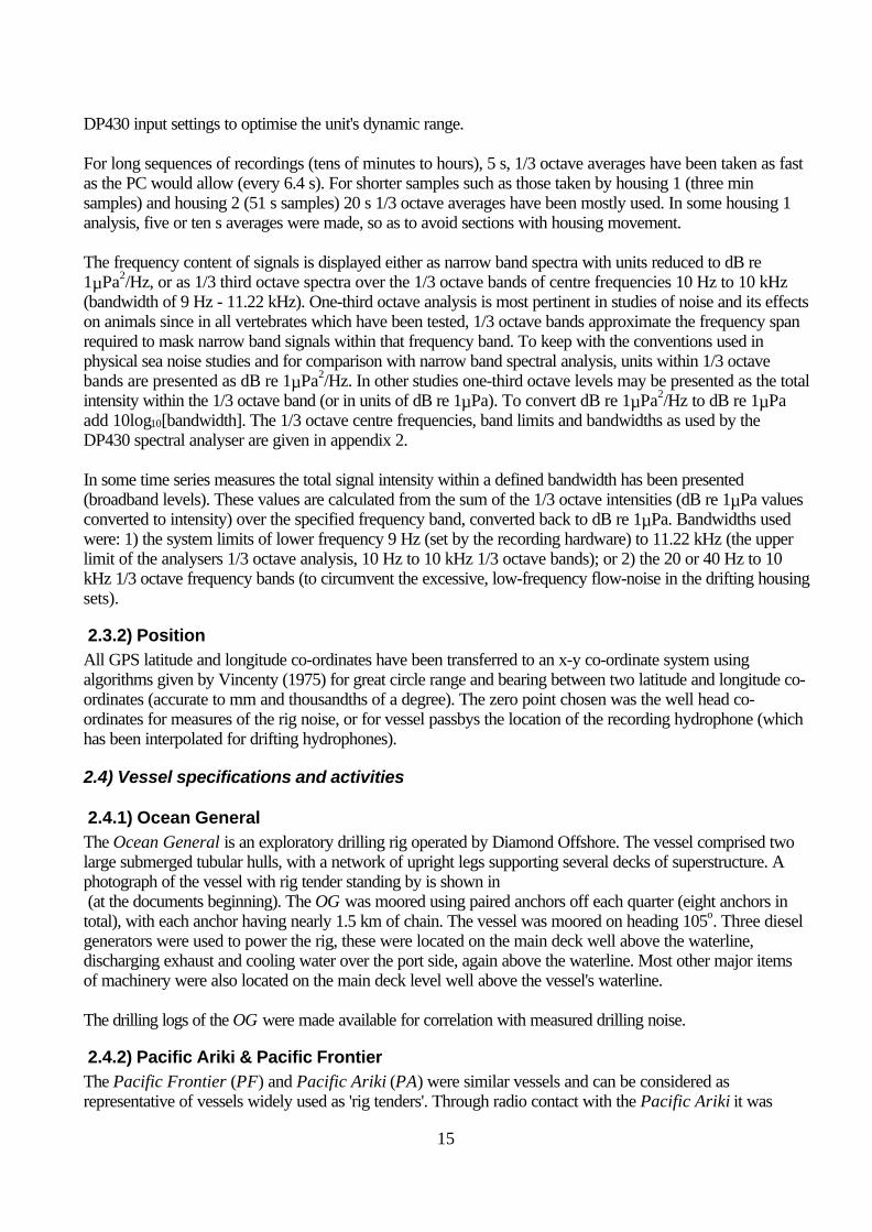
# Location Hyd. time / Equipment Drilling /depth date tender movements

A 13.7 km S OG 25 08:50 21st portable not drilling / anchoredB 22.4 km W OG 25 10:48 23rd housing 1a drilling / on stationC 22.5 km W OG 25 11:33 23rd housing 1a drilling / on stationD 13.9 km SSW OG 70 12:03 22nd housing 1 not drilling / anchoredE 13.9 km SSW OG 70 11:40 23rd housing 1 drilling / moving aboutF 13.9 km SSW OG 70 15:47 22nd housing 1 drilling / on stationG 13.9 km SSW OG 70 17:18 22nd housing 1 drilling / on station

Table 3.1: Details of the locations of ambient curves presented in Figure 7. The rig tender movements indicate wether thevessel was on anchor, moving about, or maintaining station off the rig for loading or unloading purposes (on station). Noaudible signatures, nor any spectral lines associated with the OG or rig tenders appear in the spectra.

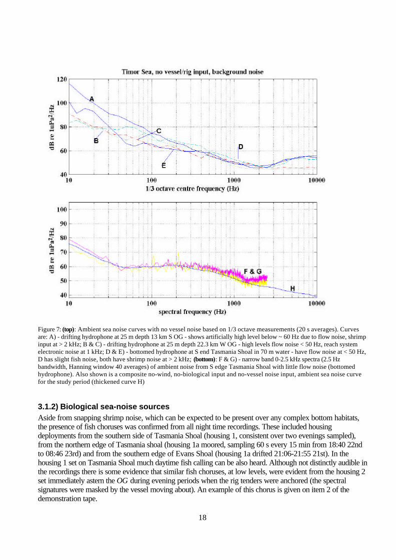
Curves B & C, taken from 22 km west of the OG in open water reached the system electronic noise atfrequencies > 2 kHz. Curves D & E taken from the back of Tasmania Shoal show similar trends to curves B& C between 100 Hz - 2 kHz, but above 2 kHz show increasing noise due to a snapping shrimp input.Snapping shrimp noise has greatest energy between 3-40 kHz, but will influence sea-noise up to 200 kHz(Cato and Bell, 1992). Curve A also shows snapping shrimp noise at > 2 kHz , and high flow noise at < 100Hz. This hydrophone was drifted from Nova at 25 m depth in 90 m water over the edge of Tasmania Shoal.

Curves F & G (Figure 7) were taken from housing 1 off the back of Tasmania Shoal and are believed to showthe lower levels of low frequency noise (< 50 Hz) encountered throughout the study. Most of the curves A-Ein Figure 7) are believed to have a significant component of flow noise at frequencies below 50 Hz, withcurves A & E showing the higher levels.

A composite curve (H) combining the low frequency portion of the bottomed hydrophone curves F & G (at <200 Hz), all curves in the mid frequencies (200 Hz - 2 kHz) and extended at the same slope above 2 kHz (toremove shrimp noise) is shown on Figure 7. This is believed to be the lowest ambient noise level which wouldhave occurred at the site over the period of measurement, correlating with environmental conditions of nowind and taken from open water regions with no snapping shrimp noise input. Small increases in wind speedand contributions from biological sources (snapping shrimp, fish, dolphins and possibly other sources) wouldgreatly increase selected portions of this curve.

The lowest levels of ambient noise in an area, along with local sound propagation effects are crucial indetermining the maximum range of audibility of any source. For long range predictions of noise audibility thecurve H presented in Figure 7 has been used. When using recordings of vessel or rig noise and calculatingreceived levels of noise, an ambient curve appropriate for the recording has been used. That is the ambientcurve used in the following estimates of received rig or vessel noise, takes into account any low frequency flownoise, as heard in all drifting recordings. For analysis of vessel noise within 10 dB of the ambient noise level ata given frequency, the contribution of the ambient noise in the received signal needs to be taken into account.For these measurements the true vessel component of the signal at the specified frequency was calculated bysubtracting the ambient intensity from the received signal intensity, and converting the value back to dB.

18

Figure 7: (top): Ambient sea noise curves with no vessel noise based on 1/3 octave measurements (20 s averages). Curvesare: A) - drifting hydrophone at 25 m depth 13 km S OG - shows artificially high level below ~ 60 Hz due to flow noise, shrimpinput at > 2 kHz; B & C) - drifting hydrophone at 25 m depth 22.3 km W OG - high levels flow noise < 50 Hz, reach systemelectronic noise at 1 kHz; D & E) - bottomed hydrophone at S end Tasmania Shoal in 70 m water - have flow noise at < 50 Hz,D has slight fish noise, both have shrimp noise at > 2 kHz; (bottom): F & G) - narrow band 0-2.5 kHz spectra (2.5 Hzbandwidth, Hanning window 40 averages) of ambient noise from S edge Tasmania Shoal with little flow noise (bottomedhydrophone). Also shown is a composite no-wind, no-biological input and no-vessel noise input, ambient sea noise curvefor the study period (thickened curve H)

3.1.2) Biological sea-noise sourcesAside from snapping shrimp noise, which can be expected to be present over any complex bottom habitats,the presence of fish choruses was confirmed from all night time recordings. These included housingdeployments from the southern side of Tasmania Shoal (housing 1, consistent over two evenings sampled),from the northern edge of Tasmania shoal (housing 1a moored, sampling 60 s every 15 min from 18:40 22ndto 08:46 23rd) and from the southern edge of Evans Shoal (housing 1a drifted 21:06-21:55 21st). In thehousing 1 set on Tasmania Shoal much daytime fish calling can be also heard. Although not distinctly audible inthe recordings there is some evidence that similar fish choruses, at low levels, were evident from the housing 2set immediately astern the OG during evening periods when the rig tenders were anchored (the spectralsignatures were masked by the vessel moving about). An example of this chorus is given on item 2 of thedemonstration tape.

19

Evening fish choruses similar to these and described as a 'popping chorus', have been described in McCauley(1995, 1997) and in McCauley and Cato (1998). Depending on several factors, such choruses can cause upto 35 dB increases in night time sea-noise levels at the chorus spectral peak. McCauley (1997) found thatalthough the choruses seem to be mostly associated with reef systems, they could often be active as far as 15km from their believed parent reef. Nocturnally active planktivorous fishes working the night time planktonlayer in shallow water depths were believed responsible for choruses.

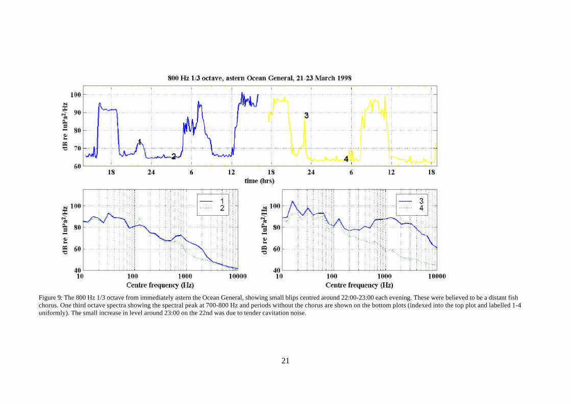
Examples of the increase in sea noise caused by such choruses are shown on Figure 8a-c. Figure 8 (top)displays the 1000 Hz 1/3 octave from the housing 1 set with time over the three day set. This curve shows aregular increase in the 1000 Hz 1/3 octave level, coincident with the fish chorus. Figure 8 bottom-left andbottom-right, show the distinctive fish chorus spectral shape in 1/3 octave measurements from the northernedge of Tasmania Shoal and the southern edge of Evans Shoal. Figure 9 (top) shows the 800 Hz 1/3 octavespectral levels from the housing sets astern the OG, with selected spectra. A regular increase in this 1/3 octaveappears between 22:00-23:00 on both evenings fully sampled (21st and 22nd). Some interference occursaround 23:00 on the 22nd from the PF moving around. It is believed these increases in the 500 Hz - 3 kHzfrequency spectra, shown on Figure 9b-c curves 2 & 3, were due to distant fish choruses. They were notclearly audible above the background OG noise in recordings.Dolphin calling was also commonly heard insea-noise records (item 3 demonstration tape). Dolphins were heard and seen at short and long ranges fromthe drilling OG.

20

Figure 8: Biological sea noise spectra over study period (21st-23rd March). Top plot shows regular presence of nightly fish chorus off the S edge of Tasmania Shoal, as indicated bythe 1000 Hz 1/3 octave spectral level with time (from the bottomed housing 2 records). This is the frequency of the chorus spectral peak (curves 3 bottom left & right). Similar choruseswere heard from the S tip of Evans Shoal on the evening of 21st (curves 1 & 2 bottom left) and off the N tip of Tasmania Shoal on the evening of the 22nd (curves 1 & 2 bottom right).From the S edge of Evans Shoal and the N edge of Tasmania Shoal rig-tender operations could be clearly heard. Curves are labelled as 1-dotted; 2-dash-dot; and 3-solid. The curves 3index into the top plot.

21

Figure 9: The 800 Hz 1/3 octave from immediately astern the Ocean General, showing small blips centred around 22:00-23:00 each evening. These were believed to be a distant fishchorus. One third octave spectra showing the spectral peak at 700-800 Hz and periods without the chorus are shown on the bottom plots (indexed into the top plot and labelled 1-4uniformly). The small increase in level around 23:00 on the 22nd was due to tender cavitation noise.

22

3.2) Rig (Ocean General) noise

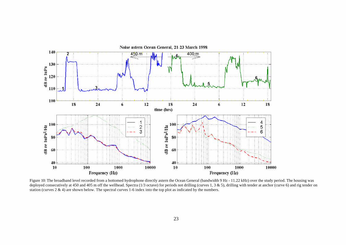
3.2.1) Ocean General and tender on station noise characterChanges in noise produced by the OG and rig tenders with time are presented in Figure 10 (top). Thispresents the total signal noise level (broadband) over the frequency span of the 1/3 octaves with centrefrequencies 10 Hz - 10 kHz, or spanning 9 Hz - 11.22 kHz. Two consecutive housing sets were made,the first at 450 m astern the rig, the second at 405 m astern. To interpret the noise produced by the OGit is necessary to detail drilling activities aboard the OG and the movements of the rig tenders. Theseactivities are given on table 3.2 from the OG drilling logs, from observations of tender movements ortender movements as recorded by the bottomed hydrophone immediately astern the OG, and throughradio contact with the rig or tender.

Table 3.2: Ocean General drilling operations and rig tender movements over study period (07:30 21st to 19:00 23rdMarch). When not actively drilling the OG was involved in various tasks, most of which involved working the drillstring or preparing the drill hole.

Date/Time OG activities Tender movts.

21st:00:00-24:00 no drillingto 15:00 PA anchored, @ 15:00 raise anchor16:05 PA at rig on station18:50 PA moves off, then anchors

22nd:03:46 PF passes S edge Tas. Shoal en-route OG, heard Hs105:00-10:00 3 hours drilling05:30-09:00 PF and PA moving about OG08:30-09:30 PA passby hyd. E Tas. Shoal, PA steams Darwin12:30-20:36 PF on station OG21:01 PF on anchor

23rd:07:30-11:00 PF moves OG, on station13:07 PF on anchor main engines shut down13:00-24:00 11 hours drilling

Not drilling noise, tender on anchorThree states of noise were recorded from the OG and associated rig-tender operations. The first statewas relatively quiet, and involved normal rig operations which did not involve drilling, with the rig tenderon anchor. These operations included working the drill string in the hole, such as reaming work, but notactive drilling. Examples of the noise produced during these periods are shown on Figure 10 (top)between: 14:00-16:00 on the 21st; 19:30 21st to 04:30 22nd; 09:30-12:00 22nd; and 21:00 22nd to07:00 23rd (item 4, demonstration tape). The configuration of the OG, with the main machinery deckwell above the waterline, probably contributed to the generally low noise output from the structure itselfduring no drilling periods.

23

Figure 10: The broadband level recorded from a bottomed hydrophone directly astern the Ocean General (bandwidth 9 Hz - 11.22 kHz) over the study period. The housing wasdeployed consecutively at 450 and 405 m off the wellhead. Spectra (1/3 octave) for periods not drilling (curves 1, 3 & 5), drilling with tender at anchor (curve 6) and rig tender onstation (curves 2 & 4) are shown below. The spectral curves 1-6 index into the top plot as indicated by the numbers.

24

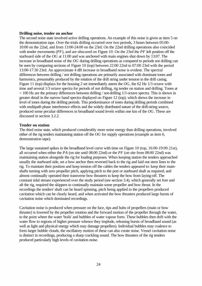
Drilling noise, tender on anchorThe second noise state involved active drilling operations. An example of this noise is given as item 5 onthe demonstration tape. Over the trials drilling occurred over two periods, 3 hours between 05:00-10:00 on the 22nd, and from 13:00-24:00 on the 23rd. On the 22nd drilling operations also coincidedwith tender movements (PF), and are obscured on Figure 10. On the 23rd the PF left position off thestarboard side of the OG at 11:00 and was anchored with main engines shut down by 13:07. Theincrease in broadband noise of the OG during drilling operations as compared to periods not drilling canbe seen by comparing sections of Figure 10 (top) between 22:00 22nd to 07:00 23rd with the period13:00-17:30 23rd. An approximate 4 dB increase in broadband noise is evident. The spectraldifferences between drilling / not drilling operations are primarily associated with dominant tones andharmonics, presumably produced by the rotation of the drill string under tension in the drill casing.Figure 11 (top) displays for the housing 2 set immediately astern the OG, the 62 Hz 1/3 octave withtime and several 1/3 octave spectra for periods of not drilling, rig tender on station and drilling. Tones at< 100 Hz are the primary differences between drilling / not-drilling 1/3 octave spectra. This is shown ingreater detail in the narrow band spectra displayed on Figure 12 (top), which shows the increase inlevel of tones during the drilling periods. This predominance of tones during drilling periods combinedwith multipath phase interference effects and the widely distributed nature of the drill-string source,produced some peculiar differences in broadband sound levels within one km of the OG. These arediscussed in section 3.2.2.

Tender on stationThe third noise state, which produced considerably more noise energy than drilling operations, involvedeither of the rig tenders maintaining station off the OG for supply operations (example as item 6,demonstration tape).

The large sustained spikes in the broadband level curve with time on Figure 10 (top, 16:00-19:00 21st),all occurred when either the PA (on site until 08:00 22nd) or the PF (on site from 08:00 22nd) wasmaintaining station alongside the rig for loading purposes. When keeping station the tenders approachedusually the starboard side, set a bow anchor then reversed back to the rig and laid out stern lines to therig. To maintain their position and keep tension off the cables the tenders appeared to: keep their main-shafts turning with zero propeller pitch, applying pitch to the port or starboard shaft as required; andalmost continually operated their transverse bow thrusters to keep the bow from laying-off. Theconstant tidal stream experienced over the study period (see section 3.4), which generally set fore andaft the rig, required the skippers to continually maintain some propeller and bow thrust. In therecordings the tenders' shaft can be heard spinning, pitch being applied to the propellers producedcavitation which can be clearly heard, and when activated the bow thrusters produced large bursts ofcavitation noise which dominated recordings.

Cavitation noise is produced when pressure on the face, tips and hubs of propellers (main or bowthruster) is lowered by the propeller rotation and the forward motion of the propeller through the water,to the point where the water 'boils' and bubbles of water vapour form. These bubbles then drift with thewater flow to regions of higher pressure whence they implode, releasing bursts of broadband sound (aswell as light and physical energy which may damage propellers). Individual bubbles may coalesce toform larger bubble clouds, the oscillatory motion of these can also create noise. Vessel cavitation noiseis distinct in recordings, producing a sharp crackling sound. The bow thrusters of the rig tendersproduced particularly high levels of cavitation noise.

25

Figure 11: The 62 Hz 1/3 octave as recorded astern the Ocean General over the 21st-23rd March. A marked increase in the level of this 1/3 octave is evident when comparing not-drilling periods (24:00-0700 23rd) to drilling periods (13:00-18:00 23rd). Bursts of vessel noise are responsible for other periods with levels > 95 dB re 1µPa2/Hz. Curves 1-4 in thebottom plots are of 1/3 octave spectra taken at the times labelled 1-6 on the top plot (52:38:10 and 62:09:53 hours are 04:38:10 and 14:09:53 on the 23rd).

26

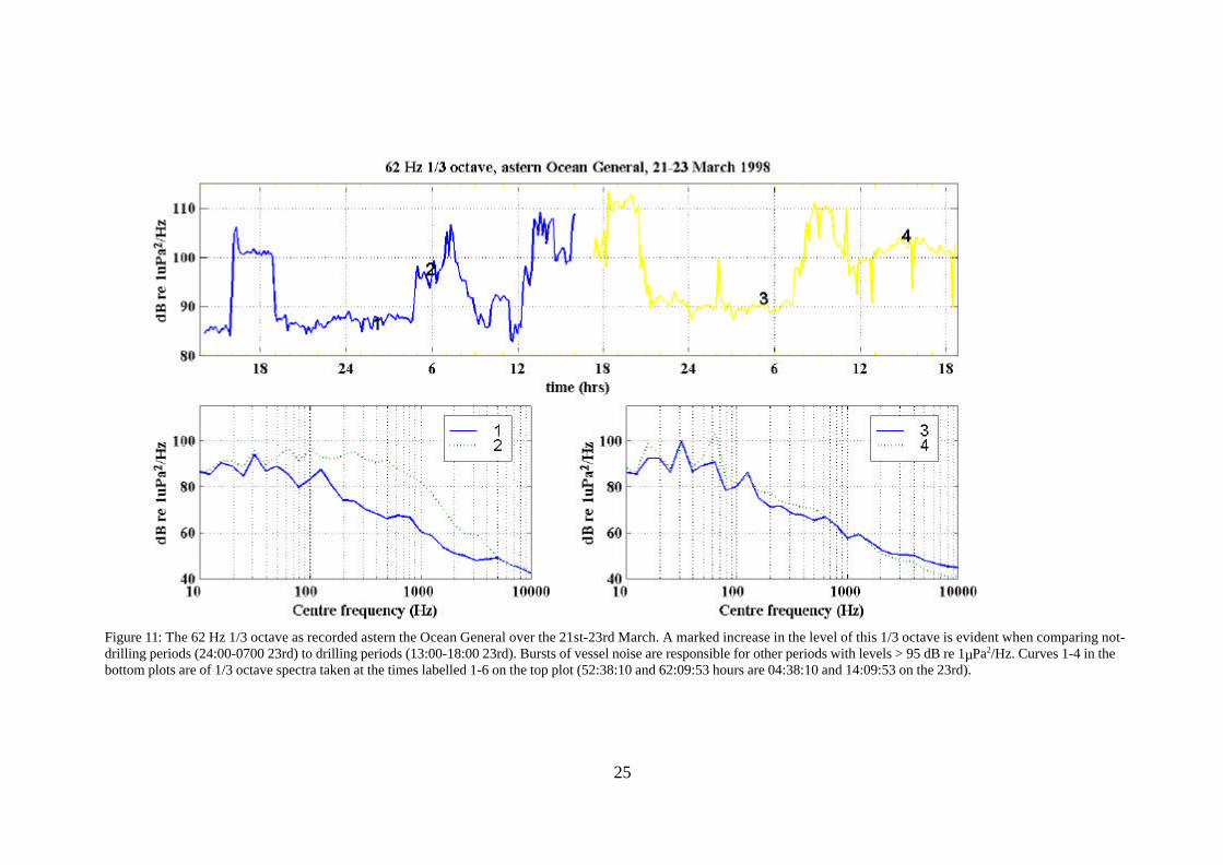
Figure 12: (top): Narrow band spectra (20 Hz-2.5 kHz, 20 averages, Hanning window, 2.5 Hz resolution) of noise from:not drilling, tender anchored main engines shut down; drilling, tender anchored main engines shut down; tender onstation noise; and ambient curve (lower thickened line). (bottom): Narrow band spectra (20 Hz - 2.5 kHz, 20 averages,Hanning window, 2.5 Hz resolution) of period of continuous drilling with tender on anchor on the 23rd, showingmeasure from 735 m N with hydrophone at 25 m depth (14:35 hrs); measure from 405 m W from bottomed hydrophone(14:54 hrs); measure from 170 m N with hydrophone at 25 m depth (14:52 hrs); and ambient curve.

Narrow band spectra of the rig not drilling, drilling and the rig tender standing by are shown on Figure12 (top) over the frequency range 20-2500 Hz. The broadband nature of the tender noise is apparent,as is the dominant tones produced during drilling, which are also apparent but not as high in level in thenot drilling spectra. Several spectra of the rig drilling (tender at anchor) at increasing range are shownon Figure 12 (bottom). An anomaly occurs in the received broadband level with range due to the 60 Hztone, this is discussed in section 3.2.2.

Underwater acoustic communications equipmentThe noise analysis presented is confined to the bandwidth of analysis, nominally 10 Hz to 11.22 kHz,although the upper system limit was 14.5 kHz. Throughout all recordings at < 1 km of the OG, constant'chirping' can be heard. This was due to the subsea communications packages used to interrogate the

27

drill head control modules. These 'chirps' would have had most energy above the bandwidth of theequipment. For most fishes these chirps would have been of little consequence. With their excellent highfrequency hearing the many dolphins in the area would have been well aware of them, and given theircuriosity some interactions between dolphins and the 'chirping' equipment may have occurred.

3.2.2) Rig noise with rangeTo interpret the noise measurements with range requires some consideration of the appropriate noisesource. During periods with the rig not drilling, no down hole work being carried out and the rig tenderat anchor, the primary noise sources will emanate from the rig. Sources will include structure bornevibration, machinery noise, pumps, valves, the noise produced by discharged exhaust or fluids, flownoise produced internally by pumping fluids about the rig and miscellaneous banging of gear beingmoved about. As the main working decks were well above the waterline much of this noise would nottransmit into the water. During this activity period the 'near field' of the source would approximate thedimensions of the rig, or roughly 100 m about the rig. In the 'near field' the noise level experienced willbe dominated by the nearest source, beyond this or in the 'far field' the many spatially separated sourceswill add together in some fashion to produce a larger noise source than experienced in the 'near field'.

During drilling operations the rig-noise will still be present, perhaps enhanced by additional machinerybought into operation to operate the rotary head and drill string, but the additional source of the drillstring rotating in the drill casing will be present. As indicated above this drill string rotation appeared toproduce several dominant tones at frequencies < 100 Hz, which also dominated measurements of thebroadband noise. During the study period the drill head depth was increased from 3,670 m below theseafloor at 00:00 on the 21st to 3,730 m at 24:00 on the 23rd. The water depth at the site was 110 m,so the drill string and casing was around 3,800 m long. Thus the source comprised the near surface rigand a 3,800 m tube, of which 3,700 m was below the seafloor, which had an internal steel pipe (drill-string) rotating in a steel (in water) or concrete (subsea) casing.

During periods with the rig tender on station the dominant noise source was cavitation produced by thetenders bow thrusters or main propellers. The vessel was 64 m long and given the thrust involved, thebubble plumes produced by the propellers would extend beyond this. Thus up to three noise sourceswere involved, rig-noise, tender-noise and the drill-string noise.

Broadband noise measurements made at various ranges from the OG during not-drilling-no-tender,drilling-no-tender and rig-tender on-station periods, are shown on Figure 13. This plot considers thebroadband level over the 1/3 octave centre frequencies 40 Hz to 10 kHz (35 Hz to 11.22 kHz bandlimits), not the 10 Hz to 10 kHz centre frequencies shown in Figure 10. This was done as most of themeasurements shown on Figure 13 were made from the Nova with a drifting hydrophone at 25 mdepth, so had some component of flow noise below 40 Hz. The broadband measurements taken fromthe housing set immediately astern the OG over the 1/3 octave centre frequencies 40 Hz - 10 kHz wereno less than 2 dB below comparable broadband measures taken over the 1/3 octave centre frequencies10 Hz to 10 kHz. On Figure 13 measurements from the bottomed hydrophone astern the OG arepresented as enlarged symbols and are calculated from the mean intensities of measurements made overthe time during which the appropriate drifting measurements were taken, expressed as a dB value.Measurements from the 25 m depth hydrophone of the drifting housing (1a) are similarly calculated.

Several measures of the ambient noise are shown, with these giving a broadband ambient level over thisfrequency band of around 93 dB re 1µPa. The idealised ambient curve H shown in Figure 7 gives anambient level of 89 dB re 1µPa over this frequency band. This level of ambient noise is believed toapproach the absolute minimum possible at the site. Increases in the ambient level due to wind, willdiminish the maximum ranges of audibility given below. Natural sea noise levels may reach to 110-115dB re 1µPa in winds of force 5-7.

28

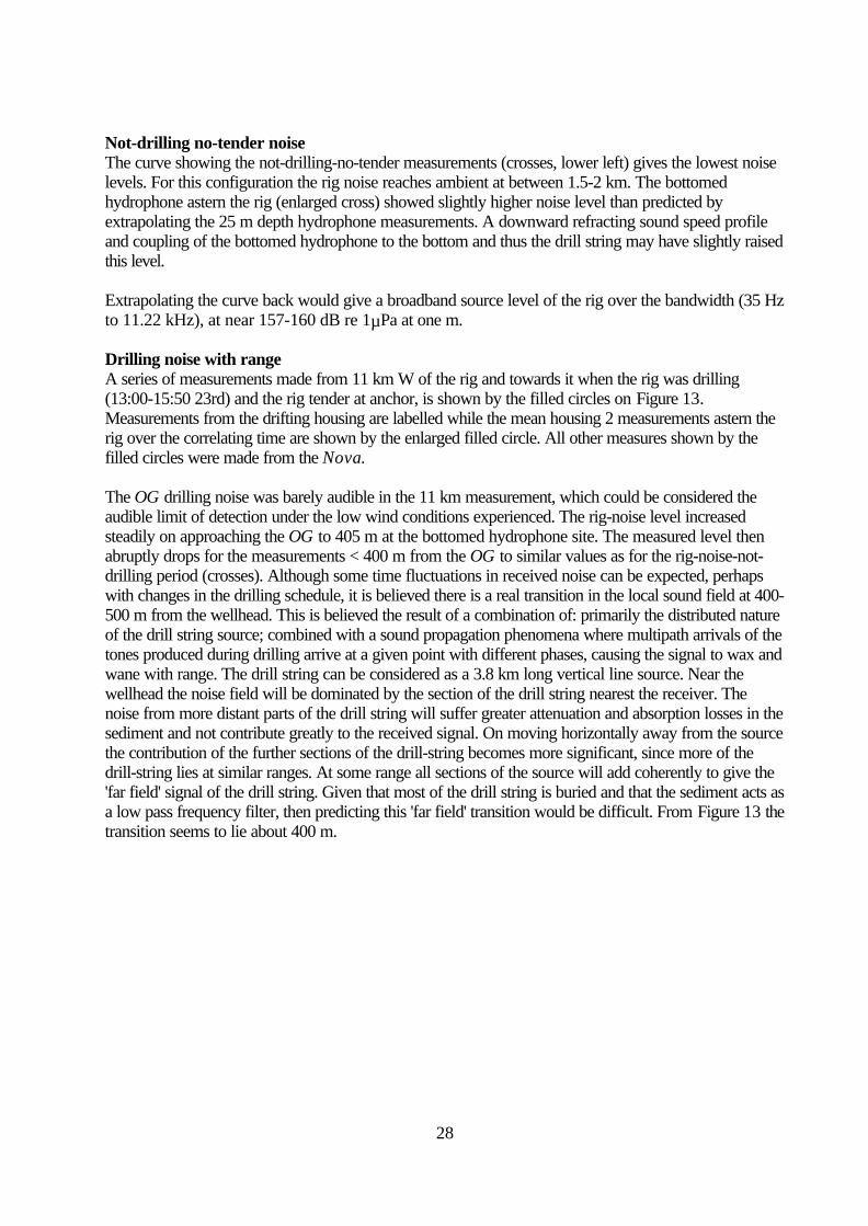
Not-drilling no-tender noiseThe curve showing the not-drilling-no-tender measurements (crosses, lower left) gives the lowest noiselevels. For this configuration the rig noise reaches ambient at between 1.5-2 km. The bottomedhydrophone astern the rig (enlarged cross) showed slightly higher noise level than predicted byextrapolating the 25 m depth hydrophone measurements. A downward refracting sound speed profileand coupling of the bottomed hydrophone to the bottom and thus the drill string may have slightly raisedthis level.

Extrapolating the curve back would give a broadband source level of the rig over the bandwidth (35 Hzto 11.22 kHz), at near 157-160 dB re 1µPa at one m.

Drilling noise with rangeA series of measurements made from 11 km W of the rig and towards it when the rig was drilling(13:00-15:50 23rd) and the rig tender at anchor, is shown by the filled circles on Figure 13.Measurements from the drifting housing are labelled while the mean housing 2 measurements astern therig over the correlating time are shown by the enlarged filled circle. All other measures shown by thefilled circles were made from the Nova.

The OG drilling noise was barely audible in the 11 km measurement, which could be considered theaudible limit of detection under the low wind conditions experienced. The rig-noise level increasedsteadily on approaching the OG to 405 m at the bottomed hydrophone site. The measured level thenabruptly drops for the measurements < 400 m from the OG to similar values as for the rig-noise-not-drilling period (crosses). Although some time fluctuations in received noise can be expected, perhapswith changes in the drilling schedule, it is believed there is a real transition in the local sound field at 400-500 m from the wellhead. This is believed the result of a combination of: primarily the distributed natureof the drill string source; combined with a sound propagation phenomena where multipath arrivals of thetones produced during drilling arrive at a given point with different phases, causing the signal to wax andwane with range. The drill string can be considered as a 3.8 km long vertical line source. Near thewellhead the noise field will be dominated by the section of the drill string nearest the receiver. Thenoise from more distant parts of the drill string will suffer greater attenuation and absorption losses in thesediment and not contribute greatly to the received signal. On moving horizontally away from the sourcethe contribution of the further sections of the drill-string becomes more significant, since more of thedrill-string lies at similar ranges. At some range all sections of the source will add coherently to give the'far field' signal of the drill string. Given that most of the drill string is buried and that the sediment acts asa low pass frequency filter, then predicting this 'far field' transition would be difficult. From Figure 13 thetransition seems to lie about 400 m.

29

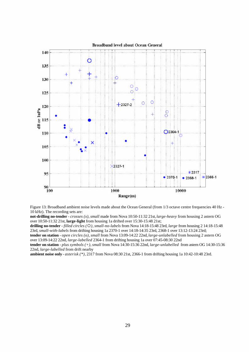
Figure 13: Broadband ambient noise levels made about the Ocean General (from 1/3 octave centre frequencies 40 Hz -10 kHz). The recording sets are:not-drilling no-tender - crosses (x), small made from Nova 10:50-11:32 21st, large-heavy from housing 2 astern OGover 10:50-11:32 21st, large-light from housing 1a drifted over 15:30-15:48 21st;drilling no-tender - filled circles (¡), small-no-labels from Nova 14:18-15:48 23rd, large from housing 2 14:18-15:4823rd, small-with-labels from drifting housing 1a 2370-1 over 14:18-14:35 23rd, 2368-1 over 13:12-13:24 23rd;tender on station - open circles (o), small from Nova 13:09-14:22 22nd, large-unlabelled from housing 2 astern OGover 13:09-14:22 22nd, large-labelled 2364-1 from drifting housing 1a over 07:45-08:30 22ndtender on station - plus symbols (+), small from Nova 14:30-15:36 22nd, large-unlabelled from astern OG 14:30-15:3622nd, large-labelled from drift nearbyambient noise only - asterisk (*), 2317 from Nova 08:30 21st, 2366-1 from drifting housing 1a 10:42-10:48 23rd.

30

A recording was made in the drifting Nova from 130 m north of the OG to 720 m NNE. This recordingstraddled the believed near-far field transition range. The section was subsequently analysed for 1/3octave levels using 5 s averages every 6.33 s. One third octave spectra at 200, 300, 500 and 650 mrange from the wellhead are shown on Figure 14a. Tones associated with drilling in the 31.25 and 62.5Hz 1/3 octaves can be seen in the spectra. Below 20 Hz the signal is dominated by flow noise. Plots ofthe 31.25 and 62.5 Hz 1/3 octaves with range are shown on Figure 14b. At less than 400 m from thewellhead the 31.25 Hz 1/3 octave waxes and wanes, as would be expected from multipath interferenceon moving away from a point source with tonal character. For a tonal point source this pattern wouldnormally continue outwards. But at 400 m the pattern changes, and although the general wax and wanetrend is evident the signal tends to flatten with increasing range, indicating additional energy is beingreceived. The 62.5 Hz 1/3 octave does not vary greatly over the 130-715 m range again indicating thatas the range increased additional energy in the 62.5 Hz 1/3 octave from the drill string below theseafloor was becoming apparent in the received signal.

The spectra shown on Figure 3.6 (bottom) also show an increase in received energy for the 60 Hzdrilling tone with increasing range out to 735 m from the wellhead. The spectra at 170 m has less energyat 60 Hz than the 405 m or 735 m spectra.

Rig tender on station noiseThe noise produced by the rig tender holding station off the rig with increasing range is shown on Figure13 by the open circles and the '+' symbols. Again measurements made during corresponding periodsfrom the housing astern the OG are shown as the larger symbols while all others were from the Nova.The symbol at 22.5 km shown as '*' was made on the 23rd with the rig tender holding station at theOG. No vessel noise could be heard in this recording. Using this record and the general trend of theopen circles curve, gives the expected maximum audible range of the tender-on-station noise as around20 km under the low wind conditions experienced.

31

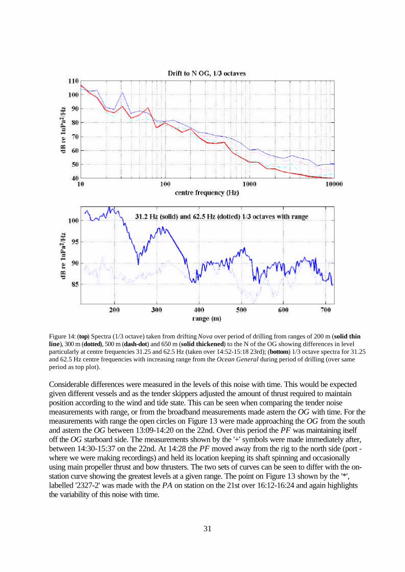
Figure 14: (top) Spectra (1/3 octave) taken from drifting Nova over period of drilling from ranges of 200 m (solid thinline), 300 m (dotted), 500 m (dash-dot) and 650 m (solid thickened) to the N of the OG showing differences in levelparticularly at centre frequencies 31.25 and 62.5 Hz (taken over 14:52-15:18 23rd); (bottom) 1/3 octave spectra for 31.25and 62.5 Hz centre frequencies with increasing range from the Ocean General during period of drilling (over sameperiod as top plot).

Considerable differences were measured in the levels of this noise with time. This would be expectedgiven different vessels and as the tender skippers adjusted the amount of thrust required to maintainposition according to the wind and tide state. This can be seen when comparing the tender noisemeasurements with range, or from the broadband measurements made astern the OG with time. For themeasurements with range the open circles on Figure 13 were made approaching the OG from the southand astern the OG between 13:09-14:20 on the 22nd. Over this period the PF was maintaining itselfoff the OG starboard side. The measurements shown by the '+' symbols were made immediately after,between 14:30-15:37 on the 22nd. At 14:28 the PF moved away from the rig to the north side (port -where we were making recordings) and held its location keeping its shaft spinning and occasionallyusing main propeller thrust and bow thrusters. The two sets of curves can be seen to differ with the on-station curve showing the greatest levels at a given range. The point on Figure 13 shown by the '*',labelled '2327-2' was made with the PA on station on the 21st over 16:12-16:24 and again highlightsthe variability of this noise with time.

32

3.3) Vessel noise

3.3.1) PropagationSound propagation at the site was estimated by using the approach and departure noise from vessels asa noise source and measuring its loss with range in 1/3 octave steps using samples which were abovethe pertinent ambient noise. This loss is expressed as a simple logarithmic loss function, or as per theequation:

Loss (dB) = β log10 (ra) 1

where β is the loss coefficient for the appropriate 1/3 octave and ra is the range in m.

Although a somewhat crude technique this is useful for vessel noise studies, in which the noise isstatistical in nature with respect to level and less so with respect to frequency content. Cavitation andbubble noise produced around propellers and in wash will vary considerably over short time scales.Thus using 1/3 octaves with time averaged samples and the log-loss approach gives some averaging tothe predicted values, with the actual level received at any range falling within some error bounds givenby the time varying nature of the source.

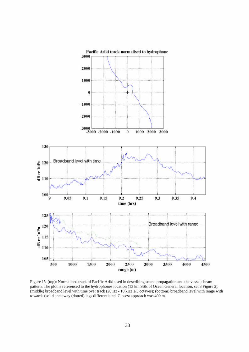
Two sets of data have been used to describe this loss. The first is from the approach and departure ofthe Pacific Ariki towards a drifting hydrophone at 25 m depth (housing 1a) made E of Tasmania Shoal(drift 3, Figure 2) on the 22nd. The PA was asked to approach the housing (surface floats with radarreflector on pole) directly to 400-500 m, to then turn in an arc around the housing, and to depart withthe housing directly astern. It was hoped to gain information on the sound propagation by using thedirect approach and depart, and of the vessels noise beam pattern by using the period during a broadturn about the hydrophone. The vessels track normalised to the hydrophone drift is shown on the topplot of Figure 15, over the period analysed for propagation and beam pattern calculations. The PAtravelled from the N (or top of plot) to S at a mean speed of 5.55 ± 0.164 ms-1 (± 95% confidencelimits), or around 11 knots, with a minimum approach range of 400 m. The broadband received signal(20 Hz to 10 kHz 1/3 octave centre frequencies) is shown on the bottom plots with time and range. Asection of the passage of the Pacific Ariki is given as item 7 on the demonstration tape.

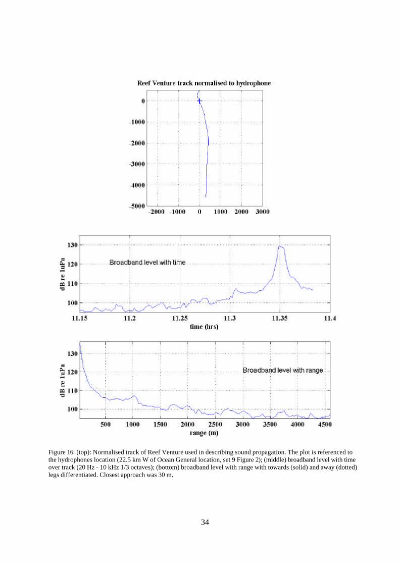
The second pass was for the Reef Venture, 22.5 km W of the OG (set 9 Figure 2) with the driftinghousing 1a and the hydrophone at 25 m depth. The section of the track used is shown on the top plot ofFigure 16 with the corresponding broadband level (20 Hz to 10 kHz 1/3 octave centre frequencies)with time and range shown underneath. The RV travelled at 6.23 ± 0.117 ms-1 or around 12.5 knots,with minimum approach range 30 m and the vessel travelling from S (bottom) to N. A section of thispassby is given as item 8 on the demonstration tape.

33

Figure 15: (top): Normalised track of Pacific Ariki used in describing sound propagation and the vessels beampattern. The plot is referenced to the hydrophones location (13 km SSE of Ocean General location, set 3 Figure 2);(middle) broadband level with time over track (20 Hz - 10 kHz 1/3 octaves); (bottom) broadband level with range withtowards (solid and away (dotted) legs differentiated. Closest approach was 400 m.

34

Figure 16: (top): Normalised track of Reef Venture used in describing sound propagation. The plot is referenced tothe hydrophones location (22.5 km W of Ocean General location, set 9 Figure 2); (middle) broadband level with timeover track (20 Hz - 10 kHz 1/3 octaves); (bottom) broadband level with range with towards (solid) and away (dotted)legs differentiated. Closest approach was 30 m.

35

For each pass the received signal was obtained in 5 s averaged 1/3 octaves from 10 Hz to 10 kHz,with a sample each 6.33 s. The program which collected the 1/3 octaves also wrote the sample starttime to file. This was used to index into the GPS files to obtain vessel range from hydrophone for eachsample. For both vessel's approach, 1/3 octaves from 25 Hz to 10 kHz were plotted with range.Approach was determined as samples where the angle of the hydrophone off the vessel's bow was lessthan 30o. For the PA, a similar curve was plotted for the departure using only points greater than 150o

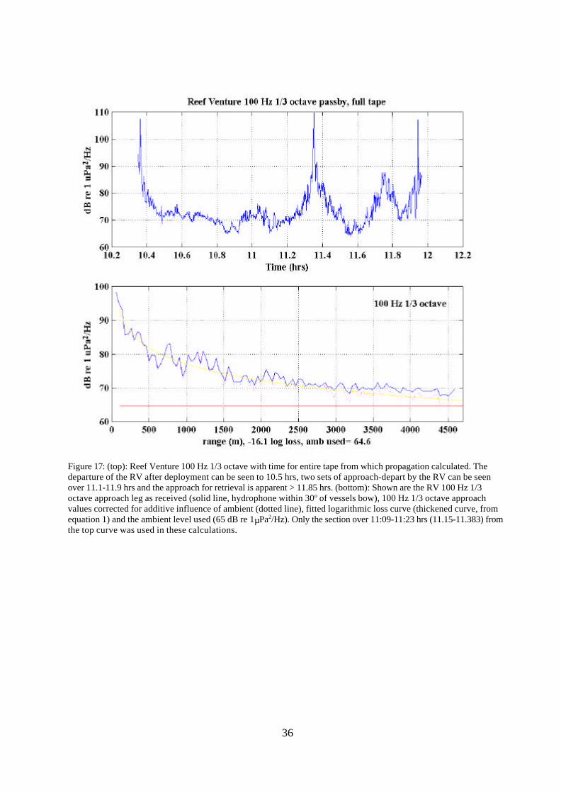
off the vessels bow (ie. hydrophone within 30o of the stern). An ambient level appropriate for this 1/3octave and recording was selected (using the entire tape's data, four hours for the PA pass, 1.75 hoursfor the RV pass). A cut off range was then determined, beyond which the appropriate 1/3 octave fellinto the ambient noise. Samples for that 1/3 octave which fell below the threshold ambient noise orabove the threshold range were removed from calculations. The resultant samples were then re-sized toremove any additive effect of the ambient noise and the log-loss equation 1 fitted to the data to give β ,or the log-loss coefficient at the appropriate 1/3 octave centre frequency. For the PA pass theapproach - departure coefficients were then averaged to give a mean value. An example of the curvesfor the 100 Hz 1/3 octave showing the full tape and the selected approach samples, the samplescorrected for additive ambient noise, and the fitted curve are shown on Figure 17.

The resultant loss coefficients for each 1/3 octave are shown onFigure 18 for the PA and RV data sets (asterisk and open circles respectively) and the mean value (+symbols). Neither set of samples had sufficient energy below the 25 Hz 1/3 octave and above thehydrophone flow noise to give accurate measurements. The separate measures are consistent, showinga gradual worsening of propagation with increasing frequency, this increasing rapidly above 2 kHz.

3.3.2) Pacific Ariki and Reef Venture noise patternsThe sound fields or beam patterns of each vessel were then described using received levels frompassbys, the frequency dependent log-loss propagation models derived above, and the lowest ambientnoise levels likely to be experienced at the site.

For the PA passby and a set of recordings of the RV moving towards and away from a driftinghydrophone on the 21st (set 3 Figure 2) the beam patterns of the vessel were calculated. These werecalculated using the received 1/3 octave levels with range. Those samples which were at less than thecut off range and greater than the threshold ambient level, as determined for the propagationmeasurements, were: adjusted for any additive ambient noise, reduced to source levels at one metreusing the frequency dependant propagation model; then plotted with angle of hydrophone off the vesselsbow (ie. no angle limits imposed). A second order polynomial was fitted with the angle-from-bow theindependent variable and the received signal level the dependant. This described the vessels sourcelevel, in 1/3 octave steps, with aspect for those aspects available from the passby geometry.

36

Figure 17: (top): Reef Venture 100 Hz 1/3 octave with time for entire tape from which propagation calculated. Thedeparture of the RV after deployment can be seen to 10.5 hrs, two sets of approach-depart by the RV can be seenover 11.1-11.9 hrs and the approach for retrieval is apparent > 11.85 hrs. (bottom): Shown are the RV 100 Hz 1/3octave approach leg as received (solid line, hydrophone within 30o of vessels bow), 100 Hz 1/3 octave approachvalues corrected for additive influence of ambient (dotted line), fitted logarithmic loss curve (thickened curve, fromequation 1) and the ambient level used (65 dB re 1µPa2/Hz). Only the section over 11:09-11:23 hrs (11.15-11.383) fromthe top curve was used in these calculations.

37

Figure 18: Mean logarithmic loss coefficients (+) for the loss of signal with range as derived empirically from equation1, using the noise of Reef Venture (o) and Pacific Ariki (*) during approach and departures as the source. The lossincreases significantly with increasing frequency as would be expected.

To plot the broadband level of each vessel as a beam pattern an x-y grid was established and from thisthe range and angle to the centre point calculated. Stepping through each 1/3 octave from 25 Hz to 10kHz: the source level for each point in the grid was calculated from the appropriate 2nd orderpolynomial of angle-from the bow with received level; the propagation loss for each point at this 1/3octave was calculated using the log-loss equation 1, and subtracted from the source level to give thereceived level at each point; the received level at each point was re-sized to include any additive effectof ambient noise (which re-sized points below the ambient noise to the ambient level); and the resultantarray was converted to intensity. Each 1/3 octave intensity was then summed, and the result convertedback to dB to give the broadband signal across the grid. Points which lay outside the geometry of thepassby were then removed. This array was then plotted as broadband level with aspect as a contourplot.

Figure 19 (top) shows the beam patterns and calculated received broadband noise for each vesselunderway (PA 11 knots, RV 12 knots) on a 20 x 20 km grid. The background ambient noise used wasthat shown on curve H, Figure 7 and can be considered as the lowest likely to be encountered at thesite. This curve gave an ambient noise of 90 dB over the 1/3 octaves 25 Hz to 10 kHz. From Figure 19it can be seen that the PA is still influencing the background noise at the extremities of the plot, althoughthe contribution at these ranges is very small given the additive effect of the background noise(accounted for in the plot calculations). This agrees well with values of the PA noise measured duringthe passby. At 9.3 km the departing PA had reached a broadband level of 103 dB re 1µPa (bandwidth25 Hz - 10 kHz 1/3 octave centre frequencies) where the recording ambient noise over this frequencyrange was estimated to be 100 dB re 1µPa (due to flow noise). In contrast the RV noise shown inFigure 19 for the vessel steaming at 12 knots, has reached well within 3 dB above the backgroundnoise an all aspects except directly ahead and astern (Figure 19 bottom plot). In recordings a toneproduced by the approaching RV can be heard at 5.5 km, but the signal is not readily audible until 5.2km. This agrees with the calculated broadband noise shown on Figure 19, where the signal would needto be at least 3 dB above the background to be audible.

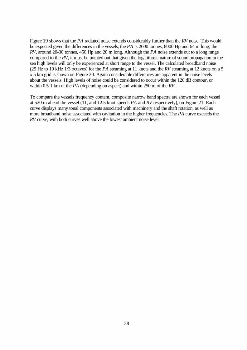
38

Figure 19 shows that the PA radiated noise extends considerably further than the RV noise. This wouldbe expected given the differences in the vessels, the PA is 2600 tonnes, 8000 Hp and 64 m long, theRV, around 20-30 tonnes, 450 Hp and 20 m long. Although the PA noise extends out to a long rangecompared to the RV, it must be pointed out that given the logarithmic nature of sound propagation in thesea high levels will only be experienced at short range to the vessel. The calculated broadband noise(25 Hz to 10 kHz 1/3 octaves) for the PA steaming at 11 knots and the RV steaming at 12 knots on a 5x 5 km grid is shown on Figure 20. Again considerable differences are apparent in the noise levelsabout the vessels. High levels of noise could be considered to occur within the 120 dB contour, orwithin 0.5-1 km of the PA (depending on aspect) and within 250 m of the RV.

To compare the vessels frequency content, composite narrow band spectra are shown for each vesselat 520 m ahead the vessel (11, and 12.5 knot speeds PA and RV respectively), on Figure 21. Eachcurve displays many tonal components associated with machinery and the shaft rotation, as well asmore broadband noise associated with cavitation in the higher frequencies. The PA curve exceeds theRV curve, with both curves well above the lowest ambient noise level.

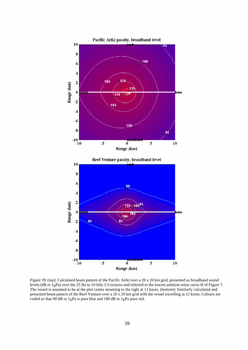
39

Figure 19: (top): Calculated beam pattern of the Pacific Ariki over a 20 x 20 km grid, presented as broadband soundlevels (dB re 1µPa) over the 25 Hz to 10 kHz 1/3 octaves and referred to the lowest ambient noise curve H of Figure 7.The vessel is assumed to be at the plot centre steaming to the right at 11 knots. (bottom): Similarly calculated andpresented beam pattern of the Reef Venture over a 20 x 20 km grid with the vessel travelling at 12 knots. Colours arecoded so that 90 dB re 1µPa is pure blue and 180 dB re 1µPa pure red.

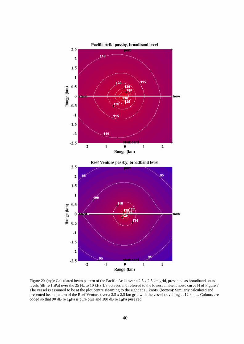
40

Figure 20: (top): Calculated beam pattern of the Pacific Ariki over a 2.5 x 2.5 km grid, presented as broadband soundlevels (dB re 1µPa) over the 25 Hz to 10 kHz 1/3 octaves and referred to the lowest ambient noise curve H of Figure 7.The vessel is assumed to be at the plot centre steaming to the right at 11 knots. (bottom): Similarly calculated andpresented beam pattern of the Reef Venture over a 2.5 x 2.5 km grid with the vessel travelling at 12 knots. Colours arecoded so that 90 dB re 1µPa is pure blue and 180 dB re 1µPa pure red.

41

Figure 21: Spectra of the Pacific Ariki and Reef Venture as received from a hydrophone directly ahead theappropriate vessel at 520 m range and compared to the lowest ambient noise spectra (curve H Figure 7). Spectra usedto obtain the plots were time averaged using a Hanning window, and 2.5 Hz resolution.

3.4) Hydrophone flow noise, CTD Casts and hydrographic regimeTen temperature, salinity and depth profiles were made over the three days on site. These were initiallytaken so as to relate with sound propagation effects. The flow noise experienced in the verticallyseparated hydrophones of housing 1a (at 25 and 75 m depth), suggested that strong differential currentflow existed in the area, with possibly surface layers travelling at a different rate and possibly directionthan sub-surface layer. Drifting recordings made in zero wind and sea conditions from the Novaindicated that there was also a very shallow differential flow component. During such recordings andwithout a drogue deployed to align the Nova drift with that of sub-surface waters, the 30 m ofhydrophone cable would often stream at a considerable angle.

Thus details of the CTD casts and the inferred hydrographic regime are presented below. The date,time, location and water depth of each site are given in table 3.3. Locations of each cast are given onFigures 2.1, 2.2 and 2.3. Profiles of temperature, salinity and computed sound speed (using theMedwin equation) are shown on Figures 3.16 and 3.17.

The ten temperature profiles were relatively consistent. In the top 5 m of water increasing surfacetemperatures were evident as the day progressed. Surface temperatures began at around 29o C early inthe day, increasing to reach as high as 30o C by late afternoon. Below 5 m depth water temperaturewas less influenced by diurnal heating, showing a steady cooling with increasing depth to around 70 m.In this layer temperature dropped at 1o C per 12-17 m of water (median drop of 1o C per 14.4 mdepth increase). Below 65-75 m and down to 100-110 m, all bar one cast displayed a stabletemperature of between 23.5-24o C. One cast (J on the 23rd at 17:30) showed a steadily decreasingtemperature profile below 60 m. Where casts were made below 100 m they show a further coolingtrend, with a near bottom temperature of 21o C recorded at site B (21st, 15:55).

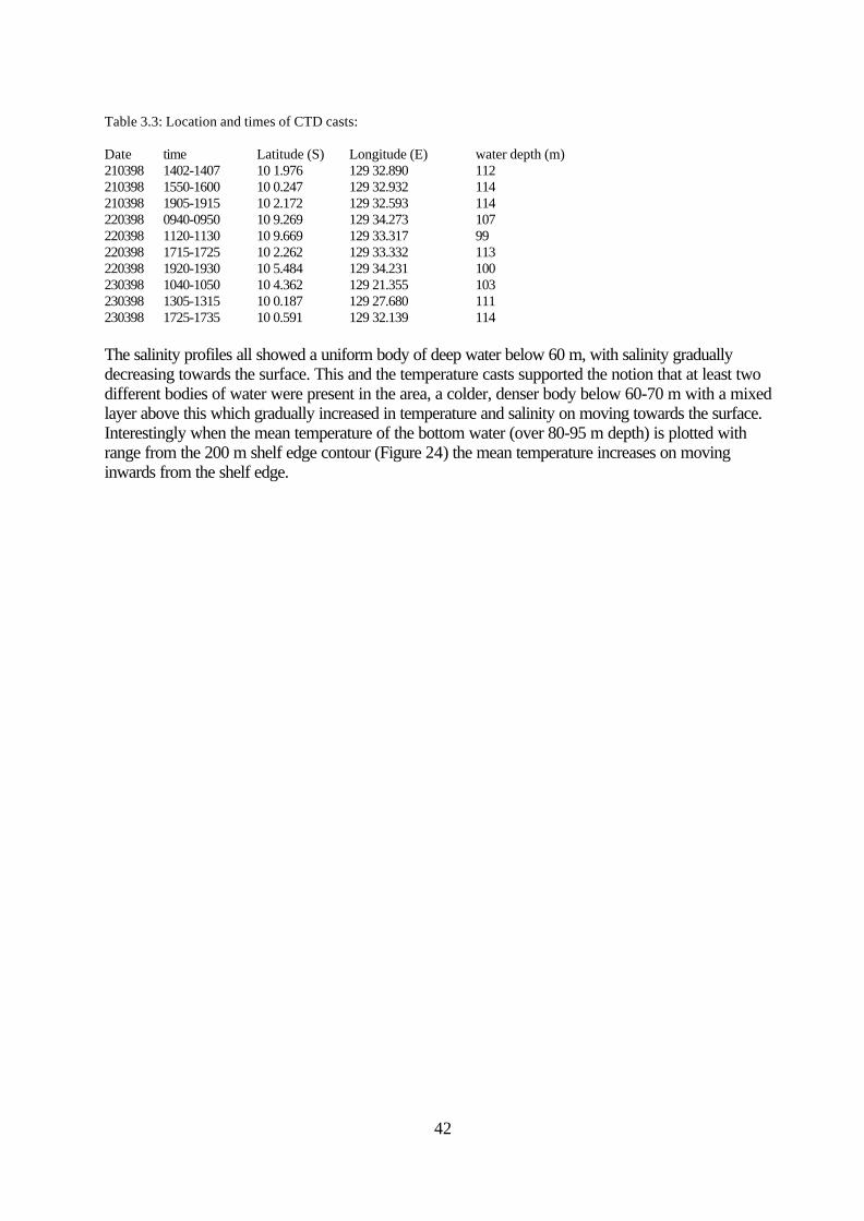
42

Table 3.3: Location and times of CTD casts:

Date time Latitude (S) Longitude (E) water depth (m)210398 1402-1407 10 1.976 129 32.890 112210398 1550-1600 10 0.247 129 32.932 114210398 1905-1915 10 2.172 129 32.593 114220398 0940-0950 10 9.269 129 34.273 107220398 1120-1130 10 9.669 129 33.317 99220398 1715-1725 10 2.262 129 33.332 113220398 1920-1930 10 5.484 129 34.231 100230398 1040-1050 10 4.362 129 21.355 103230398 1305-1315 10 0.187 129 27.680 111230398 1725-1735 10 0.591 129 32.139 114

The salinity profiles all showed a uniform body of deep water below 60 m, with salinity graduallydecreasing towards the surface. This and the temperature casts supported the notion that at least twodifferent bodies of water were present in the area, a colder, denser body below 60-70 m with a mixedlayer above this which gradually increased in temperature and salinity on moving towards the surface.Interestingly when the mean temperature of the bottom water (over 80-95 m depth) is plotted withrange from the 200 m shelf edge contour (Figure 24) the mean temperature increases on movinginwards from the shelf edge.

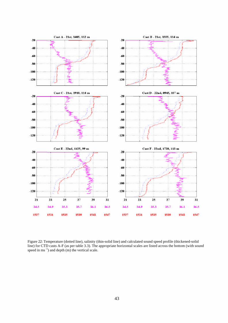
43

Figure 22: Temperature (dotted line), salinity (thin-solid line) and calculated sound speed profile (thickened-solidline) for CTD casts A-F (as per table 3.3). The appropriate horizontal scales are listed across the bottom (with soundspeed in ms -1) and depth (m) the vertical scale.

44

Figure 23: Temperature (dotted line), salinity (thin-solid line) and calculated sound speed profile (thickened-solidline) for CTD casts E-J (as per table 3.3). The appropriate horizontal scales are listed across the bottom (with soundspeed in ms-1) and depth (m) the vertical scale.

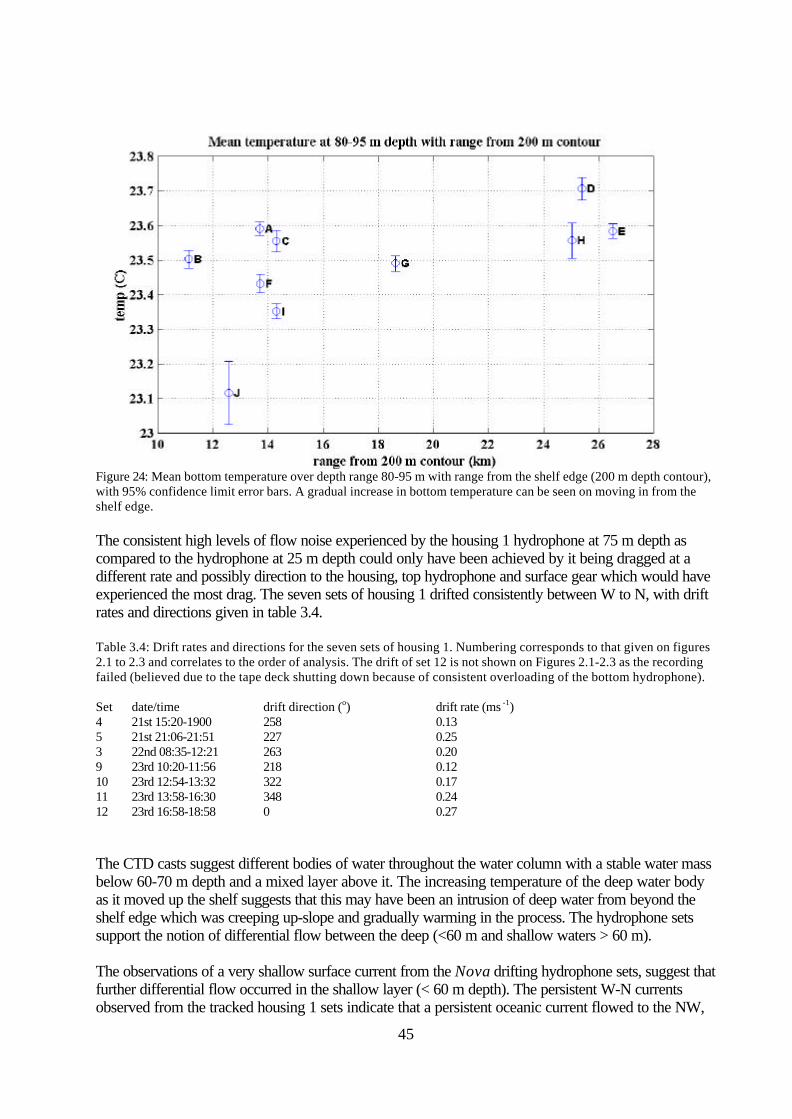
45

Figure 24: Mean bottom temperature over depth range 80-95 m with range from the shelf edge (200 m depth contour),with 95% confidence limit error bars. A gradual increase in bottom temperature can be seen on moving in from theshelf edge.

The consistent high levels of flow noise experienced by the housing 1 hydrophone at 75 m depth ascompared to the hydrophone at 25 m depth could only have been achieved by it being dragged at adifferent rate and possibly direction to the housing, top hydrophone and surface gear which would haveexperienced the most drag. The seven sets of housing 1 drifted consistently between W to N, with driftrates and directions given in table 3.4.

Table 3.4: Drift rates and directions for the seven sets of housing 1. Numbering corresponds to that given on figures2.1 to 2.3 and correlates to the order of analysis. The drift of set 12 is not shown on Figures 2.1-2.3 as the recordingfailed (believed due to the tape deck shutting down because of consistent overloading of the bottom hydrophone).

Set date/time drift direction (o) drift rate (ms -1)4 21st 15:20-1900 258 0.135 21st 21:06-21:51 227 0.253 22nd 08:35-12:21 263 0.209 23rd 10:20-11:56 218 0.1210 23rd 12:54-13:32 322 0.1711 23rd 13:58-16:30 348 0.2412 23rd 16:58-18:58 0 0.27

The CTD casts suggest different bodies of water throughout the water column with a stable water massbelow 60-70 m depth and a mixed layer above it. The increasing temperature of the deep water bodyas it moved up the shelf suggests that this may have been an intrusion of deep water from beyond theshelf edge which was creeping up-slope and gradually warming in the process. The hydrophone setssupport the notion of differential flow between the deep (<60 m and shallow waters > 60 m).

The observations of a very shallow surface current from the Nova drifting hydrophone sets, suggest thatfurther differential flow occurred in the shallow layer (< 60 m depth). The persistent W-N currentsobserved from the tracked housing 1 sets indicate that a persistent oceanic current flowed to the NW,

46

which possibly had overlaid the local tidal flow.

4) GENERAL DISCUSSIONThe production of underwater sound from the Ocean General operations has been covered by theabove results and discussion. Briefly the rig-tender when maintaining station off the rig for loadingoperations, produced the highest levels of noise which under excellent listening conditions was audibleout to 20 km (ie. Figure 13). The signal was dominated by cavitation noise produced by the vesselsmain propellers and bow thrusters, and so was broadband in nature. Comparatively high noise levels,arbitrarily defined by the broadband 120 dB re 1µPa level, extend out to around 3-5 km from the rig.Drilling and not-drilling operations when the rig tender was on anchor with main engines shut down,were considerably less noisy having a maximum audible range under ideal listening conditions of at best11 km when drilling or 1-2 km when not drilling (Figure 13). With the rig tender on anchor the noiselevels around the rig never exceeded 120 dB re 1µPa.

How these noise levels will impact on any nearby fin-fish populations is not clear based on anassessment of the literature. McCauley (1994) has reviewed the literature of noise effects on fin-fish,with respect to possible effects from offshore seismic surveys. Possible effects of high levels of man-made noise on nearby fin-fish populations could involve:

1) Attraction - There are documented studies of sharks being attracted (and repulsed) from specifictypes of noise (Myrberg et al 1976, 1978);

2) Increases in stress levels - Fish endocrine systems respond to stress with a series of hormonalinduced changes which prime the fish to deal with potential threats (reviewed in Mazeaud et al,1977). These stress responses are a normal facet of any animals life, although it is known thatchronic stress creates physiological problems such as immune suppression;

3) Disruption to any underwater acoustic cues - Acoustic signals produced by a marine animaland used in a communicative sense with other animals, or which are physical in origin but conveyenvironmental information, may be masked to some extent by continual intense noise;

4) Changes in behaviour - Levels of sound which are not sufficient to produce avoidance behaviourmay elicit behavioural changes which can potentially disrupt normal activities;

5) Localised avoidance - It is known that fish will actively avoid certain types of sound, or leave anarea in which intense sounds are being produced (Haymes and Patrick, 1986; Knudsen et al, 1992;Engås et al, 1993);

6) Abandonment of a region - It is possible that intense sound produced in an area over a long term(years) may cause abandonment of an area, although this effect is problematical and has never beenconclusively shown to occur.

For each of these possible effects there will be a gradation of severity, which may not necessarily relateto what could be considered a serious environmental or commercial impact. For example an easilyobservable effect such as localised avoidance of a sound field, may have little or no significance to ananimal from an environmental perspective. In contrast a more insidious but less obvious effect such aslong term increased stress may potentially have more severe impacts.

To assess how the noise produced by the Ocean General operations would have influenced anynearby fin-fish populations, the nature of the sound produced and the hearing capabilities of the species

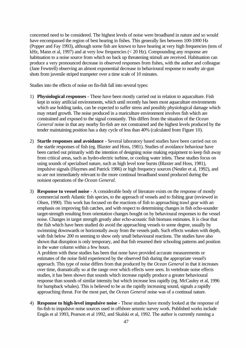
47

concerned need to be considered. The highest levels of noise were broadband in nature and so wouldhave encompassed the region of best hearing in fishes. This generally lies between 100-1000 Hz(Popper and Fay 1993), although some fish are known to have hearing at very high frequencies (tens ofkHz, Mann et al, 1997) and at very low frequencies (< 20 Hz). Compounding any response arehabituation to a noise source from which no back up threatening stimuli are received. Habituation canproduce a very pronounced decrease in observed responses from fishes, with the author and colleague(Jane Fewtrell) observing an almost exponential decrease in behavioural response to nearby air-gunshots from juvenile striped trumpeter over a time scale of 10 minutes.

Studies into the effects of noise on fin-fish fall into several types:

1) Physiological responses - These have been mostly carried out in relation to aquaculture. Fishkept in noisy artificial environments, which until recently has been most aquaculture environmentswhich use holding tanks, can be expected to suffer stress and possibly physiological damage whichmay retard growth. The noise produced in a mariculture environment involves fish which areconstrained and exposed to the signal constantly. This differs from the situation of the OceanGeneral noise in that any nearby fin-fish are not constrained and the highest levels produced by thetender maintaining position has a duty cycle of less than 40% (calculated from Figure 10).

2) Startle responses and avoidance - Several laboratory based studies have been carried out onthe startle responses of fish (eg. Blaxter and Hoss, 1981). Studies of avoidance behaviour havebeen carried out primarily with the intention of designing noise making equipment to keep fish awayfrom critical areas, such as hydro-electric turbine, or cooling water inlets. These studies focus onusing sounds of specialised nature, such as high level tone bursts (Blaxter and Hoss, 1981),impulsive signals (Haymes and Patrick 1986) or high frequency sources (Nestler et al, 1992), andso are not immediately relevant to the more continual broadband sound produced during thenoisiest operations of the Ocean General.

3) Response to vessel noise - A considerable body of literature exists on the response of mostlycommercial north Atlantic fish species, to the approach of vessels and to fishing gear (reviewed inOlsen, 1990). This work has focused on the reactions of fish to approaching trawl gear with anemphasis on improving fish catches, and with respect to determining changes in fish echo-soundertarget-strength resulting from orientation changes bought on by behavioural responses to the vesselnoise. Changes in target strength greatly alter echo-acoustic fish biomass estimates. It is clear thatthe fish which have been studied do avoid the approaching vessels to some degree, usually byswimming downwards or horizontally away from the vessels path. Such effects weaken with depth,with fish below 200 m seeming to show only small behavioural reactions. The studies have alsoshown that disruption is only temporary, and that fish resumed their schooling patterns and positionin the water column within a few hours.A problem with these studies has been that none have provided accurate measurements orestimates of the noise field experienced by the observed fish during the appropriate vessel'sapproach. This type of noise differs from that produced by the Ocean General in that it increasesover time, dramatically so at the range over which effects were seen. In vertebrate noise effectsstudies, it has been shown that sounds which increase rapidly produce a greater behaviouralresponse than sounds of similar intensity but which increase less rapidly (eg. McCauley et al, 1996for humpback whales). This is believed to be as the rapidly increasing sound, signals a rapidlyapproaching threat. For the most part, the Ocean General noise was of a continual nature.

4) Response to high-level impulsive noise - These studies have mostly looked at the response offin-fish to impulsive noise sources used in offshore seismic survey work. Published works includeEngås et al 1993, Pearson et al 1992, and Skalski et al, 1992. The author is currently running a

48

project on these types of effects. The intense but very short (mostly < 50 ms) pulses used in seismicsurveys are nothing like the noise produced by the Ocean General and so the studies are notimmediately relevant.

Given all of the above it will be difficult to accurately asses the effect of the Ocean General noise onany nearby fin-fish populations. Mitigating factors include: the low noise levels produced at times otherthan when the rig tender was maintaining station off the rig for supply operations; the low duty cycle ofthe periods of high noise levels (< 40%) and the lack of any threatening stimuli other than the noise,which will allow rapid habituation.

It is probable that during periods when the Ocean General was operating but the rig tender was onanchor, noise-effects were confined to behavioural changes within a few hundred metres of the rig.During periods when the rig-tender was maintaining station, behavioural changes may have occurred outto at least the 120 dB re 1µPa contour at 3-5 km, some avoidance may have occurred at shorterranges and nearby fish would have been aware of the vessel at up to 20 km under ideal listeningconditions.

The background noise could reach to 110 dB re 1µPa under force 5-7 conditions, at which the audiblerange of the rig with tender maintaining station would be reduced to approximately 10 km.

The recordings of fish choruses on the S edge of Evans Shoal, and the N edge of Tasmania Shoalindicated that these night-time planktivorous fishes were still active in areas insonified by the OceanGeneral noise. It is probable that partial masking of their calls would have occurred when a rig tenderwas maintaining station off the Ocean General. This noise would not have completely masked the fishsignals (source levels of the call are in the order of 154-157 dB re 1µPa p-p at one metre, McCauley1997), but may have reduced its audible range about a calling fish, to a similar range as experienced inforce 5-7 sea conditions.

The recordings of probable choruses from immediately astern the Ocean General indicate that groupsof these fishes may have been active near the rig. The slight drop in the chorus spectral peak from therecordings astern the rig as compared to choruses nearer shoals (800 Hz and 1000 1/3 octavesrespectively) are in agreement with McCauley (1997). This frequency drop was speculated to becaused as larger fish could forage further away from their daytime resting place (shoals or reefs) thansmaller fish. The swimbladder of larger fish produce lower frequency sounds than those of smaller fish,hence the lower chorus spectral peaks.

49

REFERENCESAnon (1998). Australian National Tide Tables 1998. Australian Hydrographic Publication 11,

Commonwealth of AustraliaBlaxter, J.H.S., Hoss, D.E., (1981). Startle response in herring; the effect of sound stimulus frequency,

size of fish and selective interference with the acoustico-lateralis system. J. Mar. Biol. Assoc. UK.61(4):871-880

Cato, D.H. and Bell, M.J. (1992). Ultrasonic ambient noise in Australian shallow waters at frequenciesup to 200 kHz. Defence Science and Technology Organisation, Australia, publicationMRL-TR-91-23

Cato, D.H., Tavener, S. (1997) Ambient sea noise dependence on local, regional and geostrophic windspeeds: implications for forecasting noise. Applied Acoustics 51(3):317-338

Haymes, G.T., Patrick, P.H. (1986). Exclusion of adult alewife Alosa pseudoharengus, using very lowfrequency sound for application at water intakes. Can. J. Fish. Aquat. Sci. 43:855-862

Knudsen, F.R., Enger, P.S. and Sand, O. (1992). Awareness reactions and avoidance to sound inAtlantic salmon, Salmo salar (L). Journal of Fish Biology, 40:523-534

Mann, D.A., Lu, Z., Popper, A.N. (1997). A clupeid fish can detect ultrasound. Nature 389 p. 341Mazeaud, M.M, Mazeaud, F., Donaldson, E.M. (1977) Primary and secondary effects of stress in fish:

some new data with a general review. Transactions of the American Fisheries Society106(3):201-212

McCauley, R.D. (1994). Seismic Surveys. In: Environmental implications of offshore oil and gasdevelopment in Australia - the findings of an independent scientific review, Swan, J.M., Neff, J.M.and Young, P.C. (Eds.), APEA, Sydney, pp. 19-121

McCauley, R.D. (1995). Aspects of marine biological sound production in northern Australia III: Reefassociated fish choruses. Report to DSTO, Pyrmont, NSW, from James Cook University, MarineBiology Department 39 pp.

McCauley, R.D. (1997). Aspects of marine biological sound in northern Australia IV: Fish choruses inthe GBR, spatial extent and temporal patterns. Report to DSTO from Department of MarineBiology, James Cook University, Marine Biology Department

McCauley, R.D., Cato, D.H. (1998) Evening fish choruses near coral reef systems in the Great BarrierReef Australia. Proceedings, 16th International Congress on Acoustics and 135th meetingAcoustical Society of America, pp. 1029-1030

McCauley, R.D., Cato, D.H., Jeffery, A.F. (1996). A study of the impacts of vessel noise onhumpback whales in Hervey Bay. Report for the Queensland Department of Environment &Heritage, Maryborough Office, from the Department of Marine Biology, James Cook University,Townsville, 137 pp.

Myrberg, A.A.Jr., Gordon, C.R., Kimley, A.P. (1976). Attraction of free ranging sharks by lowfrequency sound with comments on its biological significance. In (Schuijf A., Hawkins A.D., eds.)Sound reception in fish. Elsvier, New York

Myrberg, A.A.Jr., Gordon C.R., Klimley A.P. (1978). Rapid withdrawal from a sound source byopen-ocean sharks. J. Acoust. Soc. Am. 64(5):1289-1297

Nestler, J.M., Ploskey, G.R., Pickens, J. (1992). Responses of blueback herring to high frequencysound and implications for reducing entrainment at hydropower dams. North American Journal ofFisheries Management 12:667-683

Olsen, K. (1990). Fish behaviour and acoustic sampling. Rapp. P.-v. Reun. Cons. int. Explor. Mer.189:147-158

Pearson, W.H., Skalski, J.R., Malme, C.I. (1992). Effects of sounds from a geophysical survey deviceon behaviour of captive rockfish (Sebastes spp.). Can. J. Fish. Aquat. Sci. 49(7):1343-1356

Popper, A.N., Fay, R.R. (1993). Sound detection and processing by fish: critical review and majorresearch question. Brain Behav. Evol. 1993(41):14-38

Skalski J.R., Pearson W.H., Malme C.I., 1992, Effects of sounds from a geophysical device on catch

50

per unit effort in a hook and line fishery for rockfish (Sebastes spp.). Can. J. Fish. Aquat. Sci.49(7):1357-1365

Vincenty, T. (1975) Direct and inverse solutions of geodesics on the ellipsoid with applications ofnested equations. Survey Review XXII, 176:88-93

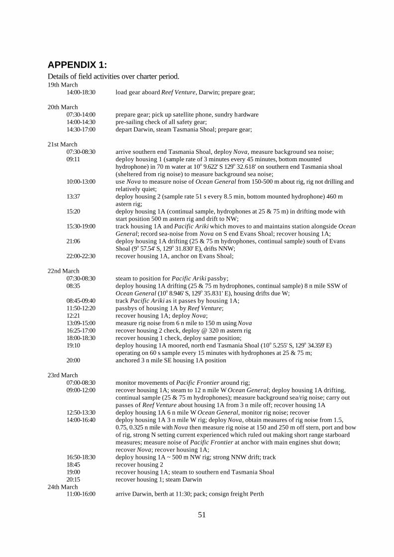
51

APPENDIX 1:Details of field activities over charter period.19th March

14:00-18:30 load gear aboard Reef Venture, Darwin; prepare gear;

20th March07:30-14:00 prepare gear; pick up satellite phone, sundry hardware14:00-14:30 pre-sailing check of all safety gear;14:30-17:00 depart Darwin, steam Tasmania Shoal; prepare gear;

21st March07:30-08:30 arrive southern end Tasmania Shoal, deploy Nova, measure background sea noise;09:11 deploy housing 1 (sample rate of 3 minutes every 45 minutes, bottom mounted

hydrophone) in 70 m water at 10o 9.622' S 129o 32.618' on southern end Tasmania shoal(sheltered from rig noise) to measure background sea noise;

10:00-13:00 use Nova to measure noise of Ocean General from 150-500 m about rig, rig not drilling andrelatively quiet;

13:37 deploy housing 2 (sample rate 51 s every 8.5 min, bottom mounted hydrophone) 460 mastern rig;

15:20 deploy housing 1A (continual sample, hydrophones at 25 & 75 m) in drifting mode withstart position 500 m astern rig and drift to NW;

15:30-19:00 track housing 1A and Pacific Ariki which moves to and maintains station alongside OceanGeneral; record sea-noise from Nova on S end Evans Shoal; recover housing 1A;

21:06 deploy housing 1A drifting (25 & 75 m hydrophones, continual sample) south of EvansShoal (9o 57.54' S, 129o 31.830' E), drifts NNW;

22:00-22:30 recover housing 1A, anchor on Evans Shoal;

22nd March07:30-08:30 steam to position for Pacific Ariki passby;08:35 deploy housing 1A drifting (25 & 75 m hydrophones, continual sample) 8 n mile SSW of

Ocean General (10o 8.946' S, 129o 35.831' E), housing drifts due W;08:45-09:40 track Pacific Ariki as it passes by housing 1A;11:50-12:20 passbys of housing 1A by Reef Venture;12:21 recover housing 1A; deploy Nova;13:09-15:00 measure rig noise from 6 n mile to 150 m using Nova16:25-17:00 recover housing 2 check, deploy @ 320 m astern rig18:00-18:30 recover housing 1 check, deploy same position;19:10 deploy housing 1A moored, north end Tasmania Shoal (10o 5.255' S, 129o 34.359' E)

operating on 60 s sample every 15 minutes with hydrophones at 25 & 75 m;20:00 anchored 3 n mile SE housing 1A position

23rd March07:00-08:30 monitor movements of Pacific Frontier around rig;09:00-12:00 recover housing 1A; steam to 12 n mile W Ocean General; deploy housing 1A drifting,

continual sample (25 & 75 m hydrophones); measure background sea/rig noise; carry outpasses of Reef Venture about housing 1A from 3 n mile off; recover housing 1A

12:50-13:30 deploy housing 1A 6 n mile W Ocean General, monitor rig noise; recover14:00-16:40 deploy housing 1A 3 n mile W rig; deploy Nova, obtain measures of rig noise from 1.5,

0.75, 0.325 n mile with Nova then measure rig noise at 150 and 250 m off stern, port and bowof rig, strong N setting current experienced which ruled out making short range starboardmeasures; measure noise of Pacific Frontier at anchor with main engines shut down;recover Nova; recover housing 1A;

16:50-18:30 deploy housing 1A ~ 500 m NW rig; strong NNW drift; track18:45 recover housing 219:00 recover housing 1A; steam to southern end Tasmania Shoal20:15 recover housing 1; steam Darwin

24th March11:00-16:00 arrive Darwin, berth at 11:30; pack; consign freight Perth

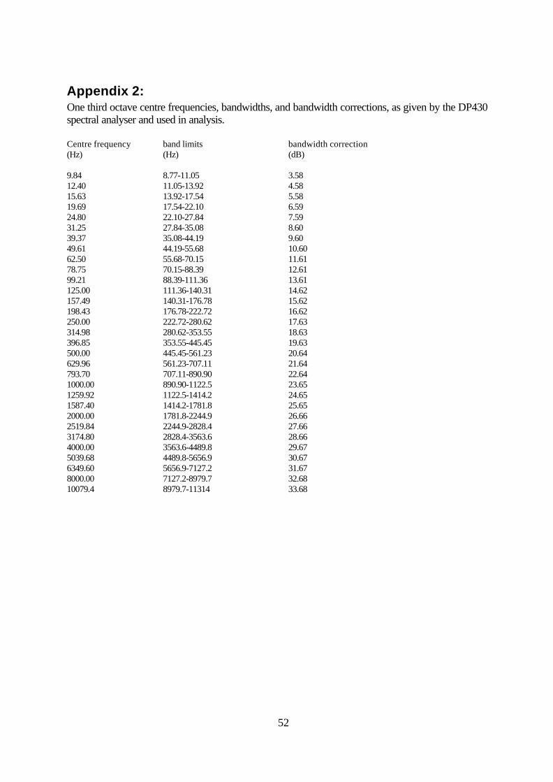
52

Appendix 2:One third octave centre frequencies, bandwidths, and bandwidth corrections, as given by the DP430spectral analyser and used in analysis.

Centre frequency band limits bandwidth correction(Hz) (Hz) (dB)

9.84 8.77-11.05 3.5812.40 11.05-13.92 4.5815.63 13.92-17.54 5.5819.69 17.54-22.10 6.5924.80 22.10-27.84 7.5931.25 27.84-35.08 8.6039.37 35.08-44.19 9.6049.61 44.19-55.68 10.6062.50 55.68-70.15 11.6178.75 70.15-88.39 12.6199.21 88.39-111.36 13.61125.00 111.36-140.31 14.62157.49 140.31-176.78 15.62198.43 176.78-222.72 16.62250.00 222.72-280.62 17.63314.98 280.62-353.55 18.63396.85 353.55-445.45 19.63500.00 445.45-561.23 20.64629.96 561.23-707.11 21.64793.70 707.11-890.90 22.641000.00 890.90-1122.5 23.651259.92 1122.5-1414.2 24.651587.40 1414.2-1781.8 25.652000.00 1781.8-2244.9 26.662519.84 2244.9-2828.4 27.663174.80 2828.4-3563.6 28.664000.00 3563.6-4489.8 29.675039.68 4489.8-5656.9 30.676349.60 5656.9-7127.2 31.678000.00 7127.2-8979.7 32.6810079.4 8979.7-11314 33.68