Radial Basis Function Networks Notes © Bill Wilson, 2009 1

Radial Basis Function Networks

Aim • to study radial basis function networks

Reference Haykin, Chapter 5 (3rd edition) or Chapter 7 (2nd ed.) provides a theoretical

treatment.

Another view is found in section 5.3 of Karray & de Silva: Soft Computing and

Intelligent Systems Design, Addison-Wesley, 2004. ISBN 0 321 11617 8

Keywords radial basis function, receptive field, hybrid learning

Plan • hybrid networks and Cover’s theorem

• define radial basis function (RBF)

• introduce RBF network

• training (estimating parameters for) RBFNs

• example

• applications

Radial Basis Function Networks Notes © Bill Wilson, 2009 2

Hybrid Networks and Cover’s Theorem

• Feedforward nets trained with backprop have all their (non-input) units homogeneous – they all

have the same activation function, and they all have the same type of training.

• Cover’s theorem (§5.2 in Haykin ed. 3), loosely speaking says that linearly inseparable patterns

are more likely to become separable if you use a non-linear transformation to map them into a

high-dimensional space. I.e. the higher the dimension, the more likely the transformed patterns

are to become separable.

• So the plan is to have a non-linear layer to transform the patterns, and then a linear layer to

separate them.

Radial Basis Function Networks Notes © Bill Wilson, 2009 3

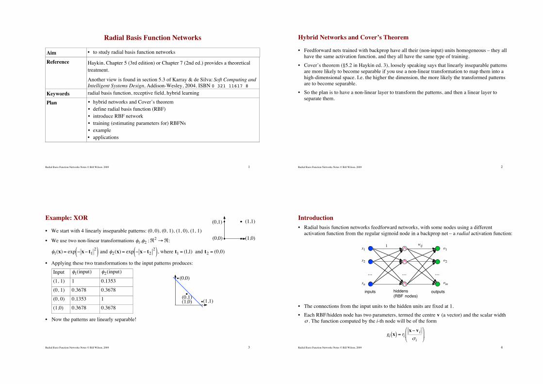
Example: XOR

• We start with 4 linearly inseparable patterns: (0, 0), (0, 1), (1, 0), (1, 1)

• We use two non-linear transformations

!

"1,"2 :#2$#:

!

"1(x) = exp # x# t12( ) and

!

"2(x) = exp # x# t22( ), where

!

t1 = (1,1) and

!

t2 = (0,0)

• Applying these two transformations to the input patterns produces:

Input

!

"1(input)

!

"2(input)

(1, 1) 1 0.1353

(0, 1) 0.3678 0.3678

(0, 0) 0.1353 1

(1,0) 0.3678 0.3678

• Now the patterns are linearly separable!

(0,1)

(0,0) (1,0)

(1,1)

(0,1)

(0,0)

(1,0) (1,1)

Radial Basis Function Networks Notes © Bill Wilson, 2009 4

Introduction

• Radial basis function networks feedforward networks, with some nodes using a different

activation function from the regular sigmoid node in a backprop net – a radial activation function:

... ... ...

inputs hiddens

(RBF nodes)outputs

1wij

x1

x2

xn

o1

o2

om

• The connections from the input units to the hidden units are fixed at 1.

• Each RBF/hidden node has two parameters, termed the centre

!

v (a vector) and the scalar width

!

" . The function computed by the i-th node will be of the form

!

gi x( ) = rix" vi

# i

$

% &

'

( )

Radial Basis Function Networks Notes © Bill Wilson, 2009 5

Radial Activation Functions

• Clearly the value of

!

gi x( ) depends on the distance of the input vector

!

x from the centre

!

vi, scaled

by the width

!

" i . All points

!

x that are equally close to

!

vi will be treated in the same way by the

function

!

gi x( ). Hence the name radial activation function.

• The most widely used radial basis function is the Gaussian function:

!

gi x( ) = exp" x" vi

2

2# i2

$

%

& &

'

(

) )

• There is no squashing function in the output neurons: the value from the j-th output unit of our

RBF network, assuming n hidden layer units and r output units, is:

!

oj (x) = wijgi(x)i=1

n

" j =1,...,r

• Another possible radial activation function is

!

gi x( ) =1

1+ exp( x" vi2/# i2).

• Note that in both cases,

!

gi(x)" 0, and so

!

oj (x)" 0, as

!

x" vi #$

Radial Basis Function Networks Notes © Bill Wilson, 2009 6

“Training” Radial Activation Functions

• Training the RBF involves estimating the best values for the

!

vi, the

!

" i , and the

!

wij.

• The standard technique is the hybrid approach, which is a two-stage learning strategy:

1) Unsupervised clustering algorithm used to find the

!

vi and

!

" i for the RBFs.

There are a number of possible clustering algorithms to try, the random input vector method,

the k-means-based method, maximum likelihood estimate-based method, standard deviations-

based method, and self-organising map method.

2) Supervised algorithm used to find values for the

!

wij.

There is only one layer with weights, so this is not as complicated as with MLPs/backprop.

We’ll describe one way to do this.

Radial Basis Function Networks Notes © Bill Wilson, 2009 7

Finding Centres and Widths: Random Input Vectors Method

• The random input vector method involves choosing the locations of centres randomly from the

training data set. All RBFs get the same width

!

" =dmax

2K, where

!

dmax is the maximum

distance between the chosen centres, and

!

K is the the number of centres.

• An alternative is to give centres differing widths depending on the local data density (broader

width if density is low).

Radial Basis Function Networks Notes © Bill Wilson, 2009 8

Finding Centres and Widths: K-means Method

• The K-means-based method is a clustering algorithm:

1 Initialise: choose several sets

!

xik| k =1,...,K{ } of random input vectors, 1 per hidden unit, and

for each set, for each input vector

!

x j, find

!

NN( j) = argminkxik

" x j . Find the set of random

input vectors that minimises

!

xNN ( j) " x jj#inputs

$2. Call this chosen set

!

tk (0) | k =1,...,K{ }. Set

n = 0. n signifies iteration number.

2 Update cluster membership: For each x ! input vectors, compute

!

kn(x) = argmink

x" tk (n) .

Thus x belongs to the cluster with centre

!

tk n( ) - this step assigns x to cluster number

!

kn(x).

!

Skn = x " inputs | kn(x) = k{ } is the set of inputs in cluster k.

3 Update cluster means: For each k, set

!

tk n+1( ) =1

Skn

x

x"Sk

n

# .

4 Continue: Add 1 to n and go to step 2. Continue until cluster memberships are stable.

• The width(s) can be done in the same way as that used for the random input vector method.

Radial Basis Function Networks Notes © Bill Wilson, 2009 9

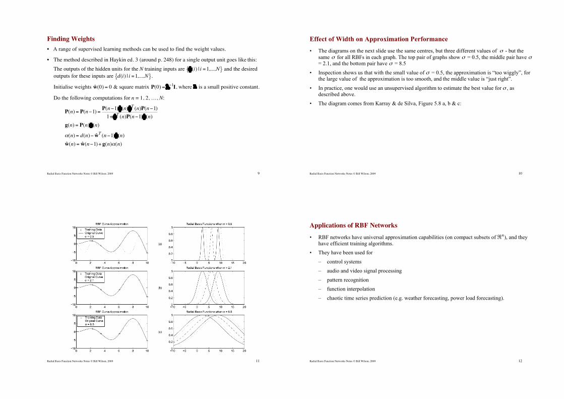
Finding Weights

• A range of supervised learning methods can be used to find the weight values.

• The method described in Haykin ed. 3 (around p. 248) for a single output unit goes like this:

The outputs of the hidden units for the N training inputs are

!

"(i) | i =1,...,N{ } and the desired

outputs for these inputs are

!

d(i) | i =1,...,N{ }.

Initialise weights

!

ˆ w (0) = 0 & square matrix

!

P(0) = "#1I, where

!

" is a small positive constant.

Do the following computations for n = 1, 2, …, N:

!

P(n) = P(n"1) =P(n"1)#(n)#T (n)P(n"1)

1+#T (n)P(n"1)#(n)

!

g(n) = P(n)"(n)

!

"(n) = d(n)# ˆ w T

(n#1)$(n)

!

ˆ w (n) = ˆ w (n"1)+ g(n)#(n)

Radial Basis Function Networks Notes © Bill Wilson, 2009 10

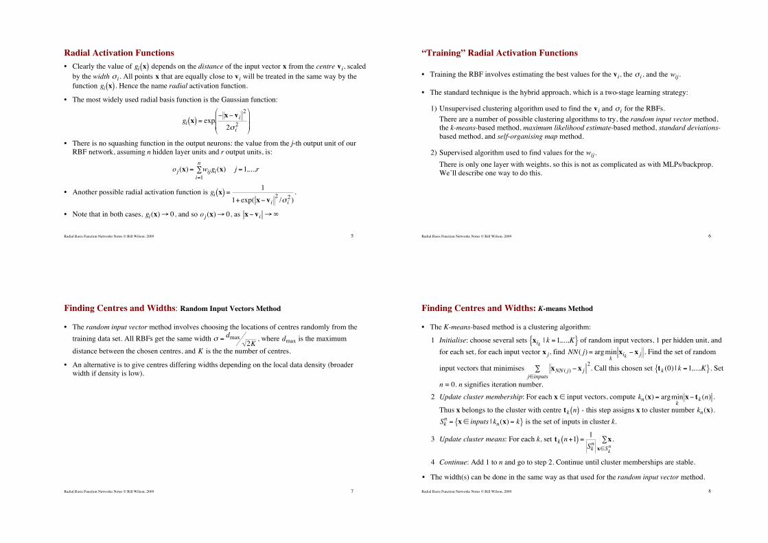
Effect of Width on Approximation Performance

• The diagrams on the next slide use the same centres, but three different values of

!

" - but the

same

!

" for all RBFs in each graph. The top pair of graphs show

!

" = 0.5, the middle pair have

!

" = 2.1, and the bottom pair have

!

" = 8.5

• Inspection shows us that with the small value of

!

" = 0.5, the approximation is “too wiggly”, for the large value of the approximation is too smooth, and the middle value is “just right”.

• In practice, one would use an unsupervised algorithm to estimate the best value for

!

" , as described above.

• The diagram comes from Karray & de Silva, Figure 5.8 a, b & c:

Radial Basis Function Networks Notes © Bill Wilson, 2009 11

Radial Basis Function Networks Notes © Bill Wilson, 2009 12

Applications of RBF Networks

• RBF networks have universal approximation capabilities (on compact subsets of

!

"n), and they

have efficient training algorithms.

• They have been used for

– control systems

– audio and video signal processing

– pattern recognition

– function interpolation

– chaotic time series prediction (e.g. weather forecasting, power load forecasting).

Radial Basis Function Networks Notes © Bill Wilson, 2009 13

David Broomhead

Professor of Applied Mathematics at UMIST and

works in applied nonlinear dynamical systems

and mathematical biology. Since the early 1980's

he has developed methods for time series

analysis and nonlinear signal processing using

techniques from nonlinear dynamics, including

modelling oculomotor control. In 1989 he was

awarded the John Benjamin Memorial Prize for

his work on radial basis function neural

networks.

D.S. Broomhead and D. Lowe. Multivariable

functional interpolation and adaptive

networks. Complex Systems, 2:321-355. 1988.