Embed Size (px)
Citation preview
C H A P T E R 0 5
KERNEL METHODS AND RADIAL BASES FUNCTIONS NETWORKS
CSC445: Neural Networks
Prof. Dr. Mostafa Gadal-Haqq M. Mostafa
Computer Science Department
Faculty of Computer & Information Sciences
AIN SHAMS UNIVERSITY
(most of figures in this presentation are copyrighted to Pearson Education, Inc.)
ASU-CSC445: Neural Networks
Prof. Dr. Mostafa Gadal-Haqq
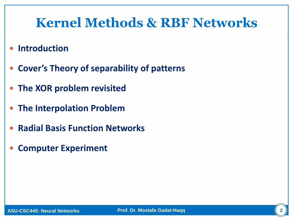
Introduction
Cover’s Theory of separability of patterns
The XOR problem revisited
The Interpolation Problem
Radial Basis Function Networks
Computer Experiment
2
Kernel Methods & RBF Networks
ASU-CSC445: Neural Networks
Prof. Dr. Mostafa Gadal-Haqq 3
Introduction
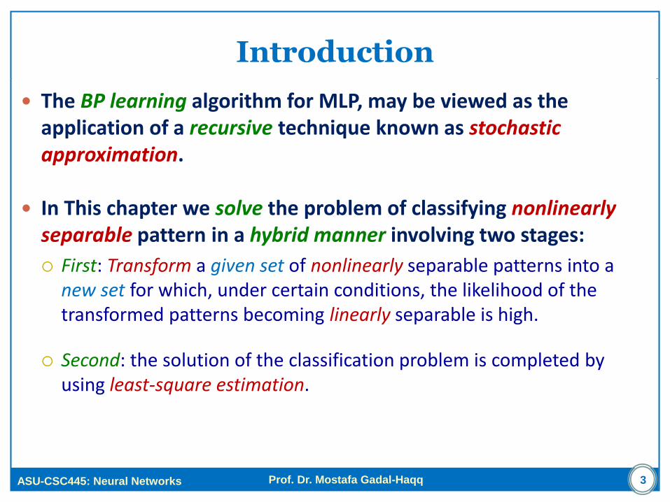
The BP learning algorithm for MLP, may be viewed as the application of a recursive technique known as stochastic approximation.
In This chapter we solve the problem of classifying nonlinearly separable pattern in a hybrid manner involving two stages:
First: Transform a given set of nonlinearly separable patterns into a new set for which, under certain conditions, the likelihood of the transformed patterns becoming linearly separable is high.
Second: the solution of the classification problem is completed by using least-square estimation.
ASU-CSC445: Neural Networks
Prof. Dr. Mostafa Gadal-Haqq 4
Cover’s Theorem
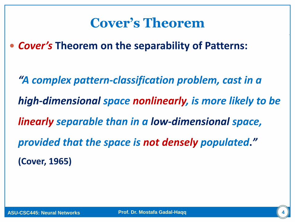
Cover’s Theorem on the separability of Patterns:
“A complex pattern-classification problem, cast in a
high-dimensional space nonlinearly, is more likely to be
linearly separable than in a low-dimensional space,
provided that the space is not densely populated.”
(Cover, 1965)
ASU-CSC445: Neural Networks
Prof. Dr. Mostafa Gadal-Haqq
Cover’s Theorem
Let X denote a set of N patterns (vectors) x1,x2,x3,…,xN; Each of which is assigned to one of two classes: C1
and C2 .
This dichotomy (binary partition) of the patterns is separable if there exist a surface that separates patterns in class C1
from those in class C2.
For each pattern x X define a vector made up of a set of real valued functions {i(x) |i=1,2,…,m1}, as
T
m )](),...,(),([)(121 xxxx
5
ASU-CSC445: Neural Networks
Prof. Dr. Mostafa Gadal-Haqq
Cover’s Theorem
If the pattern x is a vector in an m0-dimensional input space.
The vector (x) maps points in m0-dimensional input space into corresponding points in a new space of dimension m1.
We refer to i(x) as a hidden function, and the set hidden function {i(x) |i=1,2,…,m1}, is referred to as the feature space.
6
ASU-CSC445: Neural Networks
Prof. Dr. Mostafa Gadal-Haqq
Cover’s Theorem
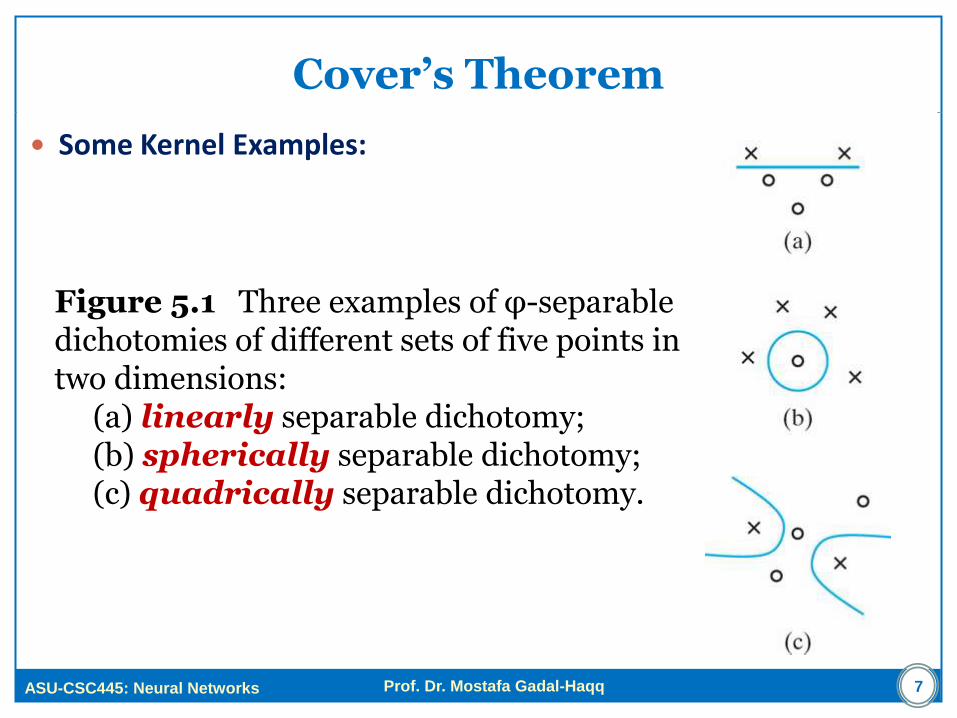
Some Kernel Examples:
Figure 5.1 Three examples of φ-separable dichotomies of different sets of five points in two dimensions: (a) linearly separable dichotomy; (b) spherically separable dichotomy; (c) quadrically separable dichotomy.
7
ASU-CSC445: Neural Networks
Prof. Dr. Mostafa Gadal-Haqq
Cover’s Theorem
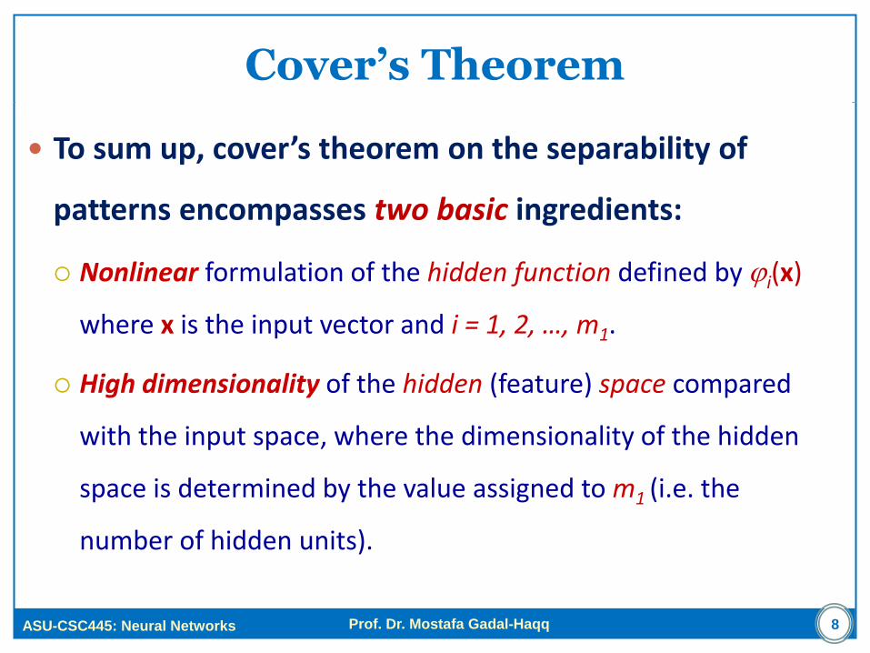
To sum up, cover’s theorem on the separability of
patterns encompasses two basic ingredients:
Nonlinear formulation of the hidden function defined by i(x)
where x is the input vector and i = 1, 2, …, m1.
High dimensionality of the hidden (feature) space compared
with the input space, where the dimensionality of the hidden
space is determined by the value assigned to m1 (i.e. the
number of hidden units).
8
ASU-CSC445: Neural Networks
Prof. Dr. Mostafa Gadal-Haqq
Cover’s Theorem
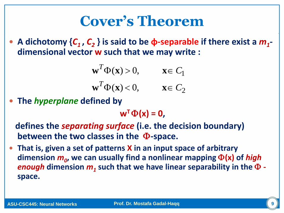
A dichotomy {C1 , C2 } is said to be φ-separable if there exist a m1-
dimensional vector w such that we may write :
The hyperplane defined by
wT (x) = 0,
defines the separating surface (i.e. the decision boundary) between the two classes in the -space.
That is, given a set of patterns X in an input space of arbitrary dimension m0, we can usually find a nonlinear mapping (x) of high enough dimension m1 such that we have linear separability in the -space.
9
2
1
,0)(
,0)(
C
C
T
T
xxw
xxw
ASU-CSC445: Neural Networks
Prof. Dr. Mostafa Gadal-Haqq
Key Idea of Kernel Methods
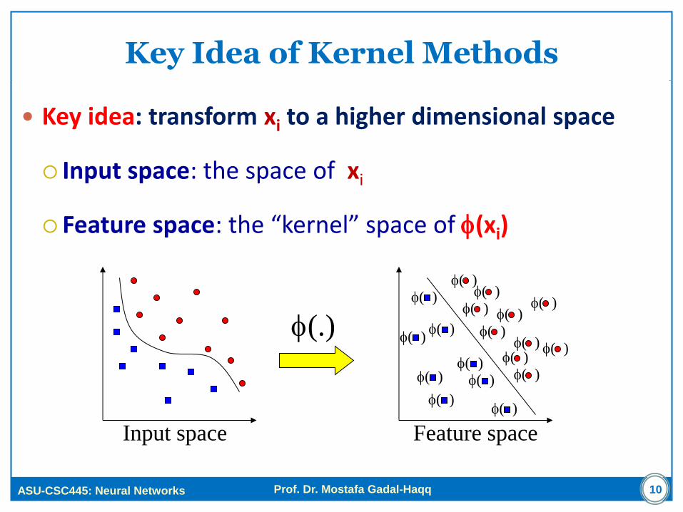
Key idea: transform xi to a higher dimensional space
Input space: the space of xi
Feature space: the “kernel” space of f(xi)
10
f( )
f( )
f( ) f( ) f( )
f( )
f( ) f( )
f(.) f( )
f( )
f( )
f( ) f( )
f( )
f( )
f( ) f( )
f( )
Feature space Input space
ASU-CSC445: Neural Networks
Prof. Dr. Mostafa Gadal-Haqq
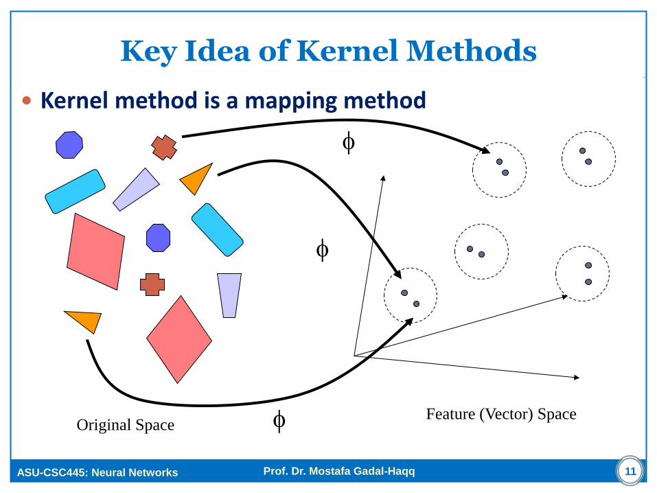
Key Idea of Kernel Methods
Kernel method is a mapping method
11
Original Space Feature (Vector) Space
f
f
f
ASU-CSC445: Neural Networks
Prof. Dr. Mostafa Gadal-Haqq
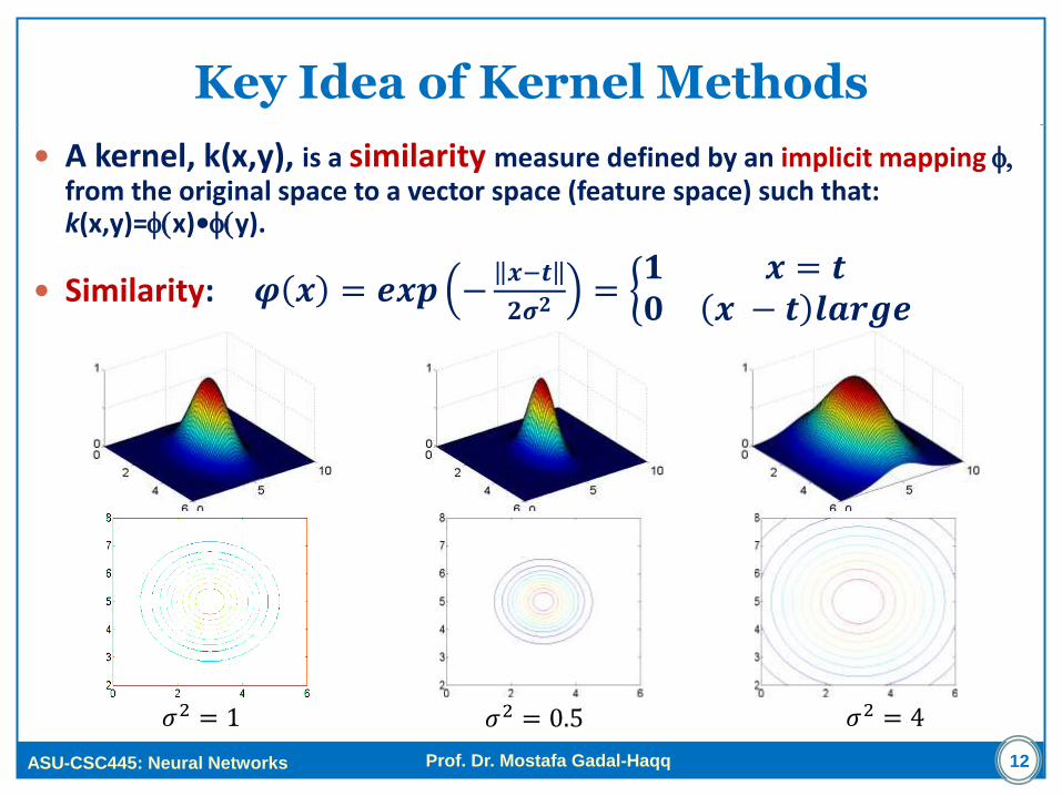
Key Idea of Kernel Methods
A kernel, k(x,y), is a similarity measure defined by an implicit mapping f, from the original space to a vector space (feature space) such that: k(x,y)=f(x)•f(y).
Similarity: 𝝋 𝒙 = 𝒆𝒙𝒑 −𝒙−𝒕
𝟐𝝈𝟐 = 𝟏 𝒙 = 𝒕𝟎 𝒙 − 𝒕 𝒍𝒂𝒓𝒈𝒆
12
𝜎2 = 1 𝜎2 = 0.5 𝜎2 = 4
ASU-CSC445: Neural Networks
Prof. Dr. Mostafa Gadal-Haqq
The XOR Problem Revisited
Recall that in the XOR problem, there are four patterns
(points), namely, (0,0),(0,1),(1,0),(1,1), in a two
dimensional input space.
We would like to construct a pattern classifier that
produces the output 0 for the input patterns (0,0),(1,1)
and the output 1 for the input patterns (0,1),(1,0).
13
ASU-CSC445: Neural Networks
Prof. Dr. Mostafa Gadal-Haqq
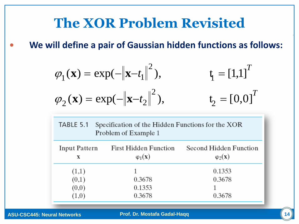
The XOR Problem Revisited
We will define a pair of Gaussian hidden functions as follows:
T
T
t
t
]0,0[ t ),exp()(
]1,1[ t ),exp()(
2
2
22
1
2
11
xx
xx
14
ASU-CSC445: Neural Networks
Prof. Dr. Mostafa Gadal-Haqq
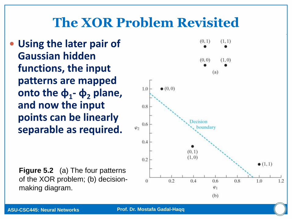
The XOR Problem Revisited
Using the later pair of Gaussian hidden functions, the input patterns are mapped onto the φ1- φ2 plane, and now the input points can be linearly separable as required.
Figure 5.2 (a) The four patterns
of the XOR problem; (b) decision-
making diagram.
ASU-CSC445: Neural Networks
Prof. Dr. Mostafa Gadal-Haqq
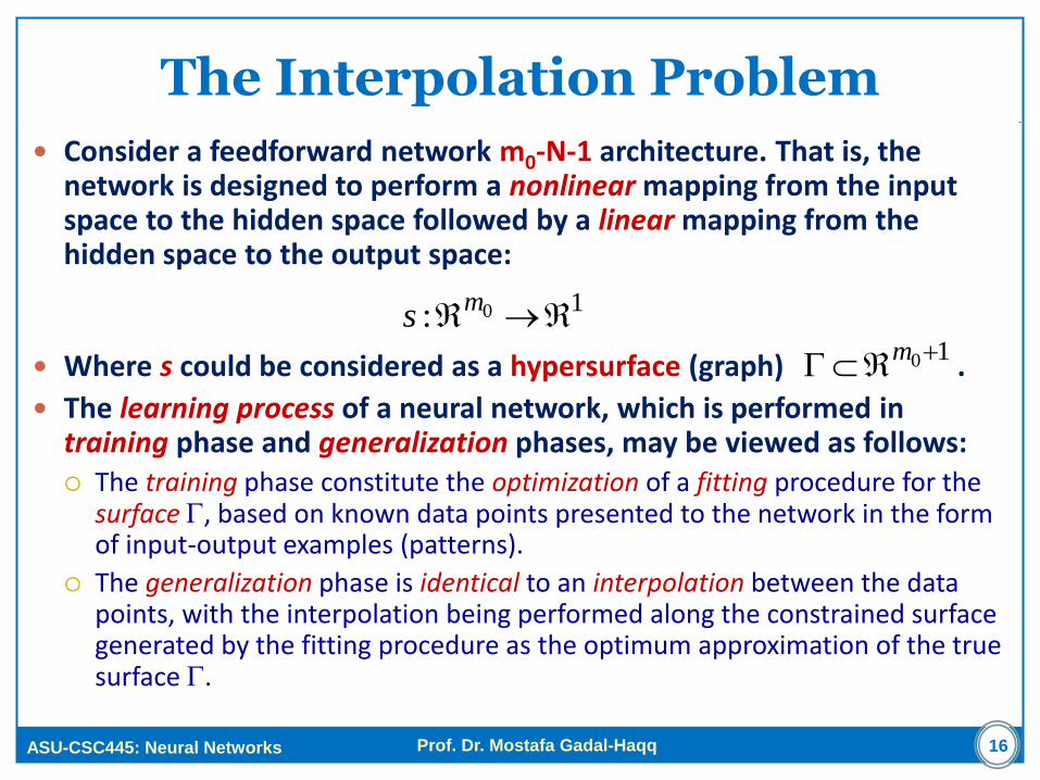
The Interpolation Problem
Consider a feedforward network m0-N-1 architecture. That is, the network is designed to perform a nonlinear mapping from the input space to the hidden space followed by a linear mapping from the hidden space to the output space:
Where s could be considered as a hypersurface (graph) .
The learning process of a neural network, which is performed in training phase and generalization phases, may be viewed as follows: The training phase constitute the optimization of a fitting procedure for the
surface , based on known data points presented to the network in the form of input-output examples (patterns).
The generalization phase is identical to an interpolation between the data points, with the interpolation being performed along the constrained surface generated by the fitting procedure as the optimum approximation of the true surface .
16
10: m
s10
m
ASU-CSC445: Neural Networks
Prof. Dr. Mostafa Gadal-Haqq
The Interpolation Problem
The interpolation problem in its strict sense, may be stated as:
Given a set of N different points and a corresponding set of real numbers , find a function , that satisfies the interpolation condition:
Strict interpolation means that the interpolation surface (i.e., the function F) is constrained to pass through all the training data points.
The radial-basis functions (RBF) technique consists of choosing a function F that has the form
Where is a set of N arbitrary (generally nonlinear) functions, known as radial-bases functions. The known data points xi are taken to be the centers of the radial-bases functions.
17
)()(1
i
N
iiwF xxx
},...,2,1|{ 0 Nim
i x},...,2,1|{ 1 Nidi
1: NF
NidF ii ,...,2,1 ,)( x
},...,2,1|)({ Nii xx
(Eq. 1)
(Eq. 2)
ASU-CSC445: Neural Networks
Prof. Dr. Mostafa Gadal-Haqq
The Interpolation Problem
Equations 1 and 2 yield a set on simultaneous linear equations of unknown coefficients (weights) {wi} given by:
Where
Let and
Let we denote the N-by-N coefficient matrix
Then, we may rewrite Eq. 3 as:
Which has the solution, assuming is nonsingular:
18
TNddd ],...,,[ 21d
NNNNNN
N
N
d
d
d
w
w
w
2
1
2
1
21
22221
11211
Njijiij ,...,2,1, ),( xx
TNwww ],...,,[ 21w
Njiij 1,}{ Φ
(Eq. 3)
dΦw
dΦw1
ASU-CSC445: Neural Networks
Prof. Dr. Mostafa Gadal-Haqq
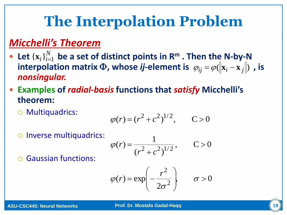
The Interpolation Problem
Micchelli’s Theorem Let be a set of distinct points in Rm . Then the N-by-N
interpolation matrix , whose ij-element is , is nonsingular.
Examples of radial-basis functions that satisfy Micchelli’s theorem: Multiquadrics:
Inverse multiquadrics:
Gaussian functions:
19
0C ,)()( 2/122 crr
)( jiij xx
Nii 1}{ x
0C ,)(
1)(
2/122
crr
0 ,2
exp)(2
2
rr
ASU-CSC445: Neural Networks
Prof. Dr. Mostafa Gadal-Haqq
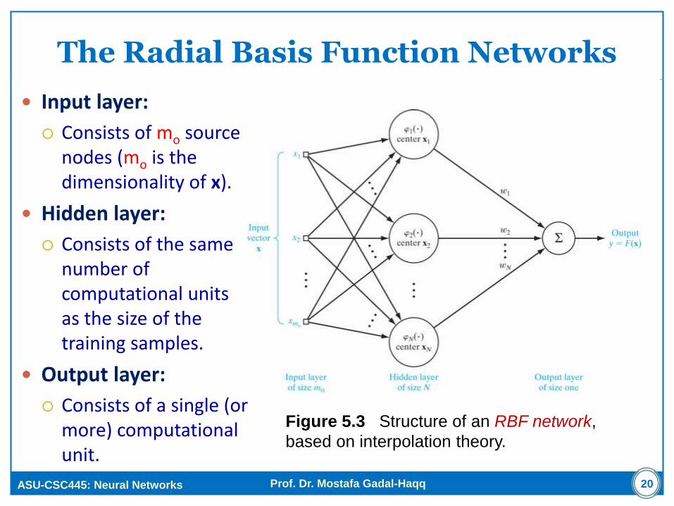
The Radial Basis Function Networks
Input layer:
Consists of mo source nodes (mo is the dimensionality of x).
Hidden layer:
Consists of the same number of computational units as the size of the training samples.
Output layer:
Consists of a single (or more) computational unit.
Figure 5.3 Structure of an RBF network,
based on interpolation theory.
20
ASU-CSC445: Neural Networks
Prof. Dr. Mostafa Gadal-Haqq
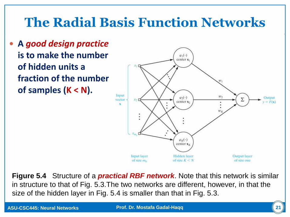
The Radial Basis Function Networks
A good design practice is to make the number of hidden units a fraction of the number of samples (K < N).
Figure 5.4 Structure of a practical RBF network. Note that this network is similar
in structure to that of Fig. 5.3.The two networks are different, however, in that the
size of the hidden layer in Fig. 5.4 is smaller than that in Fig. 5.3.
21
ASU-CSC445: Neural Networks
Prof. Dr. Mostafa Gadal-Haqq
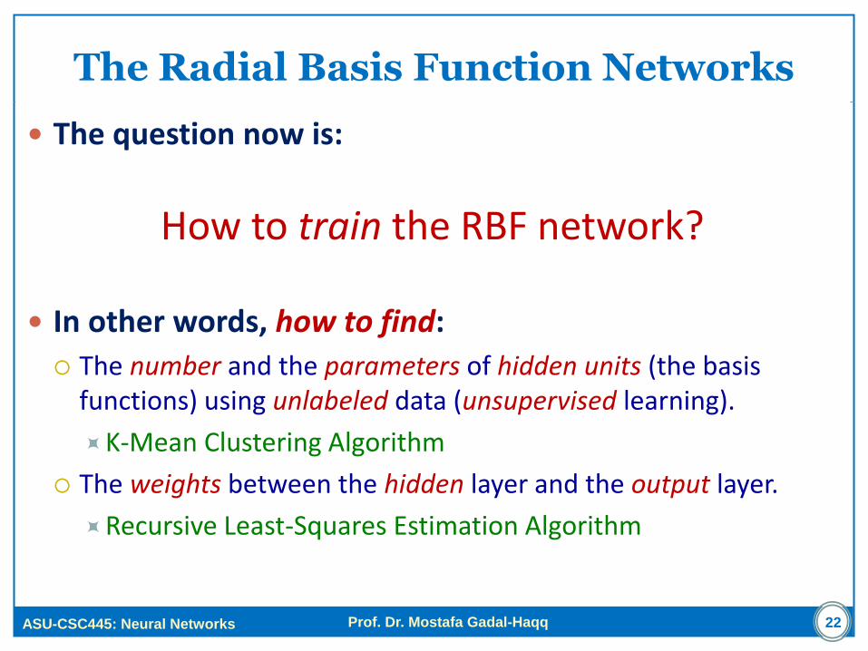
The Radial Basis Function Networks
The question now is:
How to train the RBF network?
In other words, how to find:
The number and the parameters of hidden units (the basis functions) using unlabeled data (unsupervised learning).
K-Mean Clustering Algorithm
The weights between the hidden layer and the output layer.
Recursive Least-Squares Estimation Algorithm
22
ASU-CSC445: Neural Networks
Prof. Dr. Mostafa Gadal-Haqq 23
K-Mean Clustering Algorithm
Let be a set of distinct points in Rm , which is to partitioned into set of K clusters, where K < N.
Let we have a many-to-one mapper, called the encoder, defined as:
Which assign the ith observation xi to the cluster j cluster according to a rule, yet to be defined
For example j= i mod 4, maps any number i into four clusters 0,1,2,3.
To do this encoding,
we need a similarity measure between every pair of points xi and xi’, which we denote d(xi ,xi’).
When d(xi ,xi’) is small enough, each xi and xi’ are assigned to the same cluster. Otherwise, they should belong to different clusters.
Nii 1}{ x
NiiCj ,...,2,1 )(
ASU-CSC445: Neural Networks
Prof. Dr. Mostafa Gadal-Haqq 24
K-Mean Clustering Algorithm
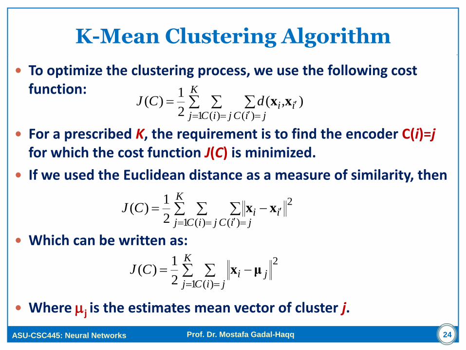
To optimize the clustering process, we use the following cost function:
For a prescribed K, the requirement is to find the encoder C(i)=j for which the cost function J(C) is minimized.
If we used the Euclidean distance as a measure of similarity, then
Which can be written as:
Where j is the estimates mean vector of cluster j.
K
j jiC jiCii,dCJ
1 )( )(
)(2
1)( xx
K
j jiC jiCiiCJ
1
2
)( )(2
1)( xx
K
j jiCjiCJ
1
2
)(2
1)( μx
ASU-CSC445: Neural Networks
Prof. Dr. Mostafa Gadal-Haqq 25
K-Mean Clustering Algorithm
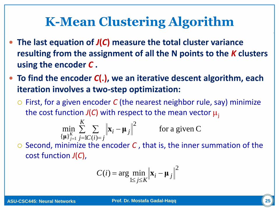
The last equation of J(C) measure the total cluster variance resulting from the assignment of all the N points to the K clusters using the encoder C .
To find the encoder C(.), we an iterative descent algorithm, each iteration involves a two-step optimization:
First, for a given encoder C (the nearest neighbor rule, say) minimize the cost function J(C) with respect to the mean vector j
Second, minimize the encoder C , that is, the inner summation of the cost function J(C),
Cgiven afor min1
2
)(}{ 1
K
j jiCjiK
j
μxμ
2
1minarg)( ji
KjiC μx
ASU-CSC445: Neural Networks
Prof. Dr. Mostafa Gadal-Haqq
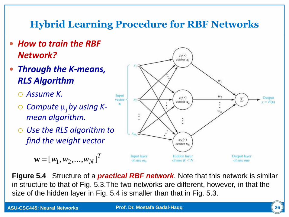
Hybrid Learning Procedure for RBF Networks
How to train the RBF Network?
Through the K-means, RLS Algorithm
Assume K.
Compute j by using K-mean algorithm.
Use the RLS algorithm to find the weight vector
Figure 5.4 Structure of a practical RBF network. Note that this network is similar
in structure to that of Fig. 5.3.The two networks are different, however, in that the
size of the hidden layer in Fig. 5.4 is smaller than that in Fig. 5.3.
26
TNwww ],...,,[ 21w
ASU-CSC445: Neural Networks
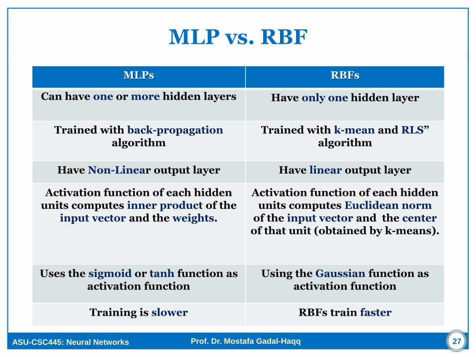
Prof. Dr. Mostafa Gadal-Haqq 27
MLP vs. RBF
MLPs RBFs
Can have one or more hidden layers Have only one hidden layer
Trained with back-propagation algorithm
Trained with k-mean and RLS” algorithm
Have Non-Linear output layer Have linear output layer
Activation function of each hidden units computes inner product of the
input vector and the weights.
Activation function of each hidden units computes Euclidean norm
of the input vector and the center of that unit (obtained by k-means).
Uses the sigmoid or tanh function as activation function
Using the Gaussian function as activation function
Training is slower RBFs train faster
ASU-CSC445: Neural Networks
Prof. Dr. Mostafa Gadal-Haqq
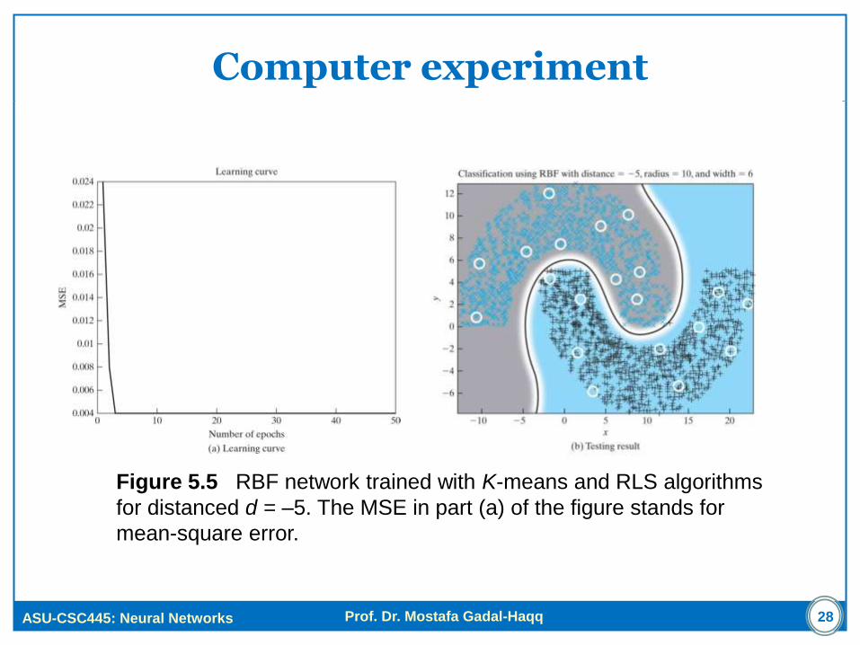
Computer experiment
Figure 5.5 RBF network trained with K-means and RLS algorithms
for distanced d = –5. The MSE in part (a) of the figure stands for
mean-square error.
28
ASU-CSC445: Neural Networks
Prof. Dr. Mostafa Gadal-Haqq
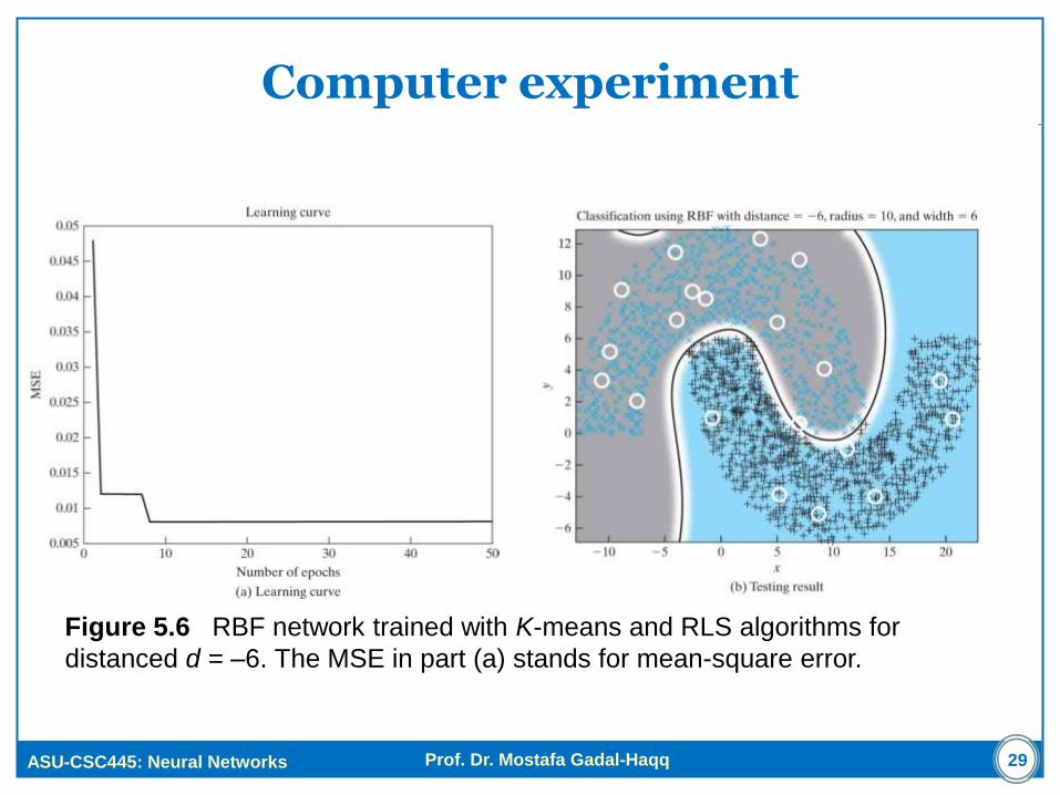
Computer experiment
Figure 5.6 RBF network trained with K-means and RLS algorithms for
distanced d = –6. The MSE in part (a) stands for mean-square error.
29
Support Vector Machines
Next Time
30