Radar and lightning analyses of gigantic jet-producing stormspeople.ee.duke.edu/~cummer/reprints/154_Meyer13_JGR_JetProducing... · Radar and lightning analyses of gigantic jet-producing

Radar and lightning analyses of gigantic jet-producing storms

Tiffany C. Meyer,1,2 Timothy J. Lang,1,3 Steven A. Rutledge,1 Walter A. Lyons,4

Steven A. Cummer,5 Gaopeng Lu,5 and Daniel T. Lindsey6

Received 16 October 2012; revised 11 February 2013; accepted 25 February 2013.

[1] An analysis of thunderstorm environment, structure, and evolution associated with sixgigantic jets (five negative polarity, one positive) was conducted. Three of these giganticjets were observed within detection range of very high frequency lightning mappingnetworks. All six were within range of operational radars and two-dimensional lightningnetwork coverage: five within the National Lightning Detection Network and one withinthe Global Lightning Detection (GLD360) network. Most of the storms producing the jetsformed in moist tropical or tropical-like environments (precipitable water ranged from 37to 62 kg m�2, and 0–6 km shear from 3.5 to 24.8 m s�1), featuring high convectiveavailable potential energy (1200–3500 J kg�1) and low lifted indices (�2.8 to �6.4). Thestorms had maximum radar reflectivity factors of 54 to 62 dBZ, and 10 dBZ echo contoursreached 14–17 km. Storms covered by three-dimensional lightning mappers were nearpeak altitude of lightning activity (modes of the vertical distributions of radio sources wereat altitudes colder than �50�C) and vertical reflectivity intensity, with overshooting echotops around the times of their jets. Two of the other three jet-producing storms producedtheir jet around the time of a convective surge as indicated by radar data and likely featuredovershooting tops. The observations suggest a link between convective surges,overshooting tops, and the occurrence of gigantic jets, similar to prior modeling studies.

Citation: Meyer, T. C., T. J. Lang, S. A. Rutledge, W. A. Lyons, S. A. Cummer, G. Lu, and D. T. Lindsey (2013), Radarand lightning analyses of gigantic jet-producing storms, J. Geophys. Res. Atmos., 118, doi:10.1002/jgrd.50302.

1. Introduction

1.1. Background

[2] All lightning—including cloud-to-ground (CG) andintracloud (IC) lightning, as well as the more uncommontransient luminous events (TLEs)—plays a role in the globalelectric circuit. Gigantic jets (GJs) are part of the TLEfamily. Like blue jets, they are thought to initiate from IC light-ning and escape upward from cloud tops. GJs extend to higheraltitude than blue jets, up to 70–90 km above mean sea level(MSL), and have a different appearance [Pasko and George,2002; Su et al., 2003; Lyons et al., 2003]. Blue jets are thoughtto form via continuous positive leader-like propagation[Wescott et al., 1998;Wescott et al., 2001]. Gigantic jets havean impulsive re-brightening characteristic resembling negativeleader processes [Pasko et al., 2002; Krehbiel et al., 2008].

[3] The first GJ was observed on 14 September 2001 bythe Lidar Laboratory of Arecibo Observatory in Puerto Rico.The GJ reached ~70 km MSL off the northwest coast fromthe main core of a relatively small thunderstorm that had acloud top of roughly 16 km [Pasko et al., 2002]. In July2002, low-light-level cameras in Kenting, Taiwan, recordedfive GJs above a 16 km tall thunderstorm over the SouthChina Sea. The jets extended to heights ranging from 86 to91 km [Su et al., 2003]. Two years later, a GJ was recordedin a frontal system over Anhui province of China, markingthe first observation over land. A few months later, severaljet-like TLEs were recorded over a thunderstorm on thecoast of Guandong province, China [Hsu et al., 2004].Two low-light cameras near Marfa, Texas, recorded the firstgigantic jet over North America on 13 May 2005. The likelyparent thunderstorm was a high-precipitation supercell clus-ter with radar echo tops of at least 14 km. Since then, moreGJs have been recorded in North America [van der Veldeet al., 2007a, 2007b]. The first positive jet was observed justwest of the island of Corsica in the Mediterranean Sea thenight of 12 December 2009. A stationary Mediterraneanwinter thunderstorm with a cloud top of only 6.5 kmproduced this GJ. The positive polarity was confirmed bythe electromagnetic waveforms observed at various radioreceiver stations [van der Velde et al., 2010].[4] In 2010, three GJs were optically detected in different

storms within detection range of ground-based, very highfrequency (VHF) networks that resolve three-dimensional(3D) lightning development. Lu et al. [2011b] examinedtwo of these jets and indicated that lightning development

1Department of Atmospheric Science, Colorado State University, FortCollins, Colorado, USA.

2Warning Decision Training Branch, National Weather Service,Norman, Oklahoma, USA.

3NASAMarshall Space Flight Center (ZP11), Huntsville, Alabama, USA.4FMA Research, Inc, Fort Collins, Colorado, USA.5Electrical and Computer Engineering Department, Duke University,

Durham, North Carolina, USA.6NOAA/NESDIS/STAR/RAMMB, Fort Collins, Colorado, USA.

Corresponding author: T. J. Lang, NASA Marshall Space Flight Center(ZP11), Huntsville, AL 35812, USA. ([email protected])

©2013. American Geophysical Union. All Rights Reserved.2169-897X/13/10.1002/jgrd.50302

1

JOURNAL OF GEOPHYSICAL RESEARCH: ATMOSPHERES, VOL. 118, 1–17, doi:10.1002/jgrd.50302, 2013

associated with these negative GJs was remarkably similarin that both jets initiated from convective cells that wereproducing normal polarity IC lightning between mid-levelnegative and upper positive charge regions. The GJs wereproduced by lightning flashes that developed as if there werea depleted upper positive charge region, as suggested byKrehbiel et al. [2008]. Table 1 shows a list of ground-based GJs observed and some of the storm characteristics.Overall, at least 24 GJs have been recorded in stormswith deep convection, consisting of >14 km echo tops and~55 dBZ reflectivity cores. Continued observations arebeing taken to capture more GJs in hopes to betterunderstand them.

1.2. Upward Lightning Formation

[5] The formation of CG and IC lightning is reasonablywell understood; however, blue jet and gigantic jet forma-tion processes are still not fully understood. Krehbiel et al.[2008] offered a hypothesis as to how upward electrical dis-charges develop from thunderstorms.[6] As the storm charges and the electric fields build up

from precipitation, discharges occur, producing differenttypes of lightning. Normally, electrified storms tend todevelop an overall negative charge imbalance with time, asa result of the negative screening charge flowing to the cloudtop [Wilson, 1921]. A �CG discharge occurs when a break-down is triggered between the mid-level negative and lowerpositive charges [Marshall et al., 2005], thereby chargingthe global electric circuit. After a �CG discharge, thestorm’s net charge becomes positive, and the electric fieldis enhanced in the upper part of the storm [Wilson, 1956].As the storm continues to charge, a discharge can be trig-gered in the upper part of the storm that can escape upward.The upward discharge would have the same polarity as the

storm, namely positive for a normally electrified storm.These upward discharges are known as blue jets [Krehbielet al., 2008].[7] Krehbiel et al. [2008] suggest a secondary mechanism

for the formation of upward discharges. Bolt-from-the-blue(BFB) discharges are classic, bi-level IC flashes, with anupward negative leader that propagates into upper levelpositive charge. If that positive charge is depleted, the leadermay exit the cloud and continue to the ground [Rison et al.,1999]. As the BFB exits the cloud, it may be “guided” byinferred positive screening charge attracted to the lateralcloud boundaries by the mid-level negative charge [Krehbielet al., 2008]. In the case of a negative gigantic jet, there is no“guiding” so the preferred discharge mode of the IC flashwith a depleted upper positive charge is upward. In a normalpolarity thunderstorm, the negative GJ effectively dischargesthe mid-level negative storm charge.[8] Blue jets contribute to charging of the global electric

circuit, whereas negative GJs weaken the circuit [Su et al.,2003]. For the case of an inverted electrified storm, withpositive charge near mid-levels, a negative blue jet orpositive gigantic jet may be produced instead. In this case,the positive GJ would contribute to the global circuit.

1.3. Overview of the Present Study

[9] Given the relative rarity of GJ observations, the mete-orological context for their occurrence is not well known.Most GJs observed in past studies developed from intense,tall thunderstorms [Pasko et al., 2002; Su et al., 2003;van der Velde et al., 2007a; Soula et al., 2011]. A reasonablehypothesis is that intense thunderstorms undergoing convec-tive surges may provide favorable characteristics for thedevelopment of GJs; as such, thunderstorms often featureturbulent mixing and overshooting tops that could disrupt

Table 1. Ground-Based Gigantic Jet Observationsa

Date Place L/W Storm TypeCloud Top

(km)Jet Height

(km) Reference Notes

15 Sep 2001 200 km NW of Puerto RicoWater Thunderstorm Cell 16 87-91 Pasko et al., 200222 Jul 2002 ~500 km SSW of Kenting,

TaiwanWater Thunderstorm Cell 16 86-91 Su et al., 2003 5 events between 1409 and

1421 UTC18 Jun 2004 ~700 km from Anhui

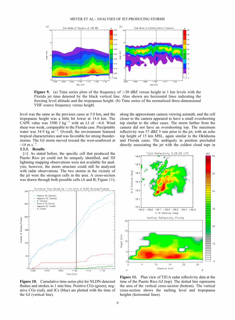
province of ChinaLand Frontal System ? ? Hsu et al., 2004

3 Aug 2004 ~500 km from Guandongprovince, China

Coast Thunderstorm Cell ? 70 Hsu et al., 2004 Possible gigantic jet

13 May 2005 Northern Mexico Land High PrecipitationSupercell

14 69-80 van der Velde etal., 2007a

22 July 2007 Fujian Province, China Land Thunderstorm Cell 15 ≥65 Chou et al. 2011 Originated as blue starter/jet20 Aug 2007 Missouri Land Multicell Thunderstorm 15-16 94 & 83 van der Velde et

al., 2007bProduced 2 jets and a sprite

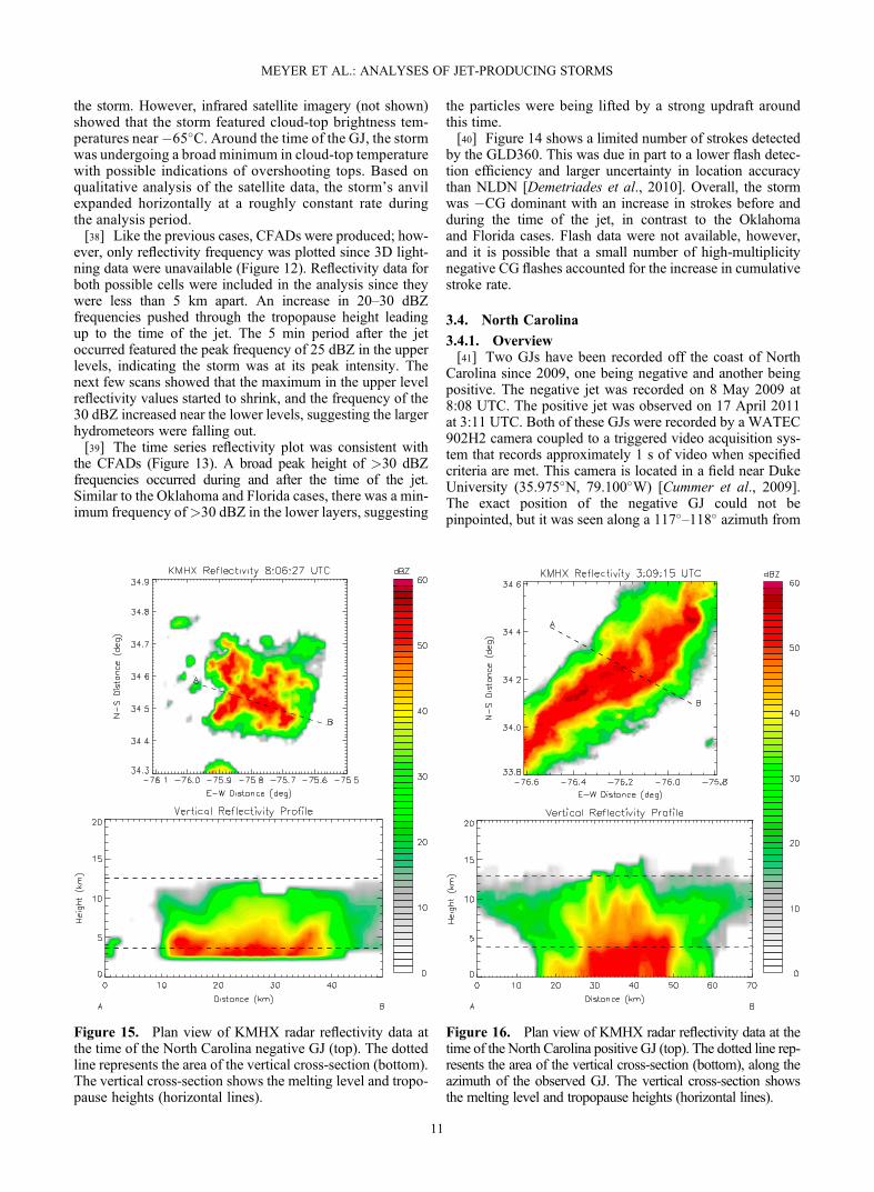
21 Jul 2008 Off coast near Duke Water Tropical Storm (TS)Cristobal

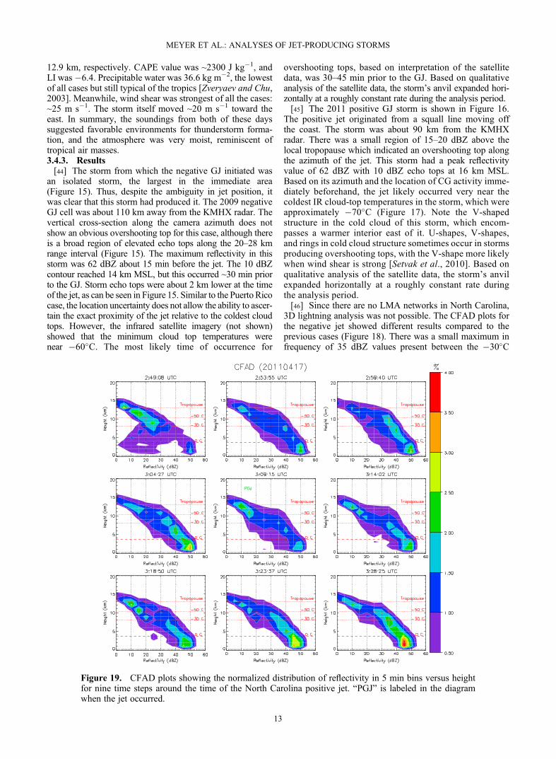
15 88 Cummer et al.,2009

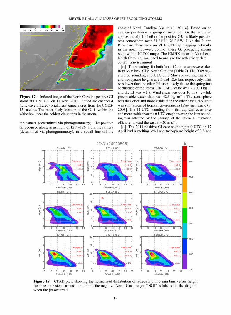
8 May 2009 Off coast near Duke Water Isolated cell12 Dec 2009 West of Corsica Water Stationary winter

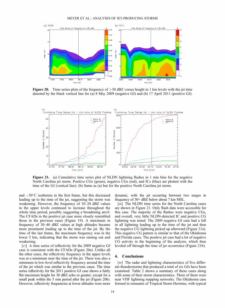
thunderstorm6.5 91 Van der Velde et

al., 2010First +GJ produced ~50TLEs

7 Mar 2010 East of Reunion Island Water Isolated tropical storm ? 80-90 Soula et al., 2011 5 events between 1740 and1829 UTC

9 Sep 2010 Eastern OK Land TS Hermine 15 90 Lu et al., 2011b 2 events in 10 minutes28 Sep 2010 205 km from Sebring, FL Water Convective Cell

(Remnants of TS)16.2 80 Lu et al., 2011b First jet to ascend into

daytime ionosphere17 Apr 2011 NC Water Squall line supercell 15 ? Lu et al., 2011a Positive GJ22 Sep 2011 Puerto Rico Land Convective cell in a

tropical airmass15 ? Lyons (2012)*

URSI talk

aHighlighted in grey are the cases examined in this study.

MEYER ET AL.: ANALYSES OF JET-PRODUCING STORMS

2

the upper charge layers through depletion or displacement ofthe negative upper screening layer and the main upper posi-tive charge region [Riousset et al., 2010].[10] Gigantic jets are far less common than convective

surges and overshooting tops, so this should be thought ofas a potentially necessary condition for GJ developmentrather than a sufficient one. The idea is that disruption ofthe upper charge regions through convective surges andovershooting tops make GJ occurrence more likely, ratherthan assuring their occurrence. Thus, GJs should be morecommon when storms are undergoing convective surgesand during times when overshooting tops are present.[11] In order to test this hypothesis, the meteorological

contexts for six gigantic jets were examined. Three negativeGJs occurred within 3D VHF lightning mapping networks:two in Oklahoma and one in Florida. Lu et al. [2011b]looked at one of the Oklahoma jets and the Florida GJ. Afourth negative GJ in Puerto Rico, a negative jet off the coastof North Carolina, and a positive jet also off the coast ofNorth Carolina also were analyzed. The last three jets werenot within 3D lightning mapping range, but two-dimensional (2D) lightning data were analyzed. An analysisof the meteorological environments and radar-observedstorm structures was performed for all six GJs.

2. Data and Methodology

2.1. Overview

[12] Lightning, radar, and sounding data were used to an-alyze the storms producing gigantic jets in this study. Twodifferent ground-based 2D lightning networks were used aswell as two 3D VHF lightning mapping networks. For eachstorm, data from the closest radar were obtained, and thesounding profile at a time and location close to the jetwas analyzed. Since the jets have only been recorded vialow-light cameras at night, visible satellite data—criticalfor identifying overshooting tops—was not useful. How-ever, infrared satellite imagery was examined.

2.2. Two-Dimensional Lightning Networks

2.2.1. National Lightning Detection Network[13] Vaisala’s National Lightning Detection Network

(NLDN) has been detecting the electromagnetic radiationfrom lightning return strokes and providing detailed light-ning data for the entire continental United States since1989 [Cummins et al., 1998; Orville, 2008]. Up until 2006,only CG lightning flashes were reported by the NLDN; how-ever, previous studies had shown that severe storms producemuch higher rates of IC lightning than CG [MacGorman andNielsen, 1991; Williams et al., 1999; Wiens et al., 2005].Thus, in the early 2000s, NLDN sensors were modified toallow improved detection of large-amplitude, very lowfrequency/low frequency (VLF/LF) pulses by IC flashes[Cummins and Murphy, 2009]. Lightning information onlocation, amplitude (peak current), and polarity is recordedfor each stroke within a flash (CG or IC). A flash is definedby Cummins and Murphy [2009] as the ensemble of all CGstrokes that strike within 10 km of each other within a 1 sinterval. The NLDN has a detection efficiency up to 95%and location accuracy <500 m for CG lightning, while ICflash detection efficiency is on the order of 25–30%[Cummins and Murphy, 2009].

2.2.2. Global Lightning Dataset (GLD360)[14] In 2009, Vaisala’s Global Lightning Dataset

(GLD360) was launched as a ground-based, lightning-detection network capable of providing worldwide coverage.The network consists of long-range VLF sensors andbecame fully operational in May 2011. GLD360 data havea 70% CG flash detection efficiency and a 5–10 km medianCG stroke location accuracy [Demetriades et al., 2010]. Thenetwork reports peak current (Ipk) and polarity estimates butdoes not classify the strokes as CG or IC [Said et al., 2010];however, a classification of |Ipk|> 7 kA and |Ipk|< 7 kA forCGs and ICs, respectively [Holle, 2009], was used foridentification in this study.

2.3. Three-Dimensional Lightning Mapping Networks

2.3.1. Oklahoma Lightning Mapping Array[15] The Lightning Mapping Array (LMA) was developed

at the New Mexico Institute of Mining and Technology[Krehbiel et al., 2000] and was modeled after the LightningDetection and Ranging (LDAR) system developed for theKennedy Space Center (KSC) [Maier et al., 1995]. TheLMA detects VHF radiation emitted by leaders duringdevelopment of a lightning flash [Rison et al., 1999]. Thesystem is able to map total lightning activity, including ICand CG lightning, in all three spatial dimensions as a functionof time. While 3D mapping is best done within 100 km rangeof network center, both the horizontal and altitude locationdata have proven to be scientifically useful even beyond 200km range [MacGorman et al., 2008; Lang et al., 2010, 2011;Lu et al., 2011b].2.3.2. Four-Dimensional Lightning Surveillance System[16] The Four-Dimensional Lightning Surveillance Sys-

tem (4DLSS) represents an upgrade and merger of theLDAR system [Lennon and Maier, 1991] and the Cloud-to-Ground Lightning Surveillance System (CGLSS) [Boydet al., 2005] at KSC in Florida. The LDAR component con-sists of nine VHF antennas that sense impulsive emissionsfrom lightning in the 60–66 MHz range [Roeder, 2010].Similar to the Oklahoma LMA, the LDAR system detectsIC lightning and produces a full 3D spatial mapping of light-ning discharge activity. The CGLSS system uses similarsensors to the NLDN [Biagi et al., 2007] to detect CGflashes [Murphy et al., 2008].

2.4. Radar, Satellite, and Sounding Data

[17] For each storm, nearby NEXRAD Level II radar datawere obtained from the has.ncdc.noaa.gov website. For allscans ranging from 30 min before to 30 min after the jet, thelatitude and longitude points of a polygon that surroundedthe entire storm which produced the jet were identified usingtheWarning Decision Support System-II (WDSS-II) software.The minimum box size used (Puerto Rico case) was approxi-mately 20 km by 20 km, and the maximum size used was 20km by 40 km (Oklahoma case). Focus was placed on onlythe core (or possible cores, if jet location was ambiguous) thatproduced the GJ, and on following that core as it moved byshifting the box location in time.[18] Two different methods were used to interpolate the

data to a grid. The first involved using the National Centerfor Atmospheric Research SPRINT radar data interpolationsoftware. This software interpolates radar measurementstaken in spherical coordinates and converts them to regularly


3

http://has.ncdc.noaa.gov

spaced latitude-longitude grids in height [Mohr and Vaughn,1979]. When necessary to fill in missing data, the WDSS-IIsoftware was used. WDSS-II was developed by the NationalSevere Storms Laboratory to manipulate radar data[Lakshmanan et al., 2007; Hondl, 2003]. WDSS-II was usedto input Level II WSR-88D data and create mosaic data froma single radar by transforming the data into latitude, longi-tude, and height grids [Lakshmanan et al., 2006]. The outputfor both of these methods was grids with reflectivity data ateach 0.01� (~1 km) in the horizontal and 1 km in the vertical.[19] Longwave infrared satellite imagery from the Geosta-

tionary Operational Environmental Satellites (GOES) wasexamined for each of the cases, around the times of the jets.Locations of GJs were compared to the locations of the coldestcloud tops. Atmospheric sounding data were taken from theclosest site. The temperature and dewpoint vertical profileswere looked at as well as convective available potential energy(CAPE), lifted index (LI), and wind shear values.

3. Gigantic Jet Cases

[20] The GJ observations are reported below by the geo-graphic location in which they occurred. Two GJs occurredin Oklahoma, one in Florida, one in Puerto Rico, and twooffshore near North Carolina. Each case is summarized byobservations, environmental conditions, and discussion. Theseinclude where and when the jet occurred, the atmosphericsoundings around the time of the jet, the evolution of the storm,and radar and electric structure via cross-sections, contouredfrequency by altitude diagrams, and time series plots.

3.1. Oklahoma

3.1.1. Overview[21] Two negative GJs were recorded in eastern Oklahoma

on 9 September 2010 at 7:22 UTC and 7:28 UTC, respec-tively. The GJs were observed from Hawley, Texas(32.66�N, 99.84�W) from a Watec 902H2 camera stampedwith exact Global Positioning System time ~500 km awayfrom the storm, and GJ locations were fixed via queryingthe Oklahoma LMA data near the times of the GJs [Luet al., 2011b]. A negative sprite also was observed at 6:49UTC in this storm [Lu et al., 2012], though not examinedin this study. The GJs were within 225 km of the center ofthe Oklahoma LMA [MacGorman et al., 2008]. This is alittle far for optimal 3D mapping, but the upper lightningstructure was still resolved. Two-dimensional NLDN dataalso were available for this storm.3.1.2. Environment[22] The storm producing the two negative jets was a

strong thunderstorm embedded in the remnants of TropicalStorm Hermine. Hermine developed off the coast of south-eastern Mexico five days prior to the jet observations. Manytornado, wind, and flooding reports were recorded through-out Texas and Oklahoma as Hermine made its way inland(reports may be found at http://www.spc.ncep.noaa.gov/exper/archive/events/searchindex.html). Hermine was stillconsidered a tropical depression when the GJ-producingstorm formed. The environment was very moist andtropical-like. The 0 UTC sounding from Norman, Oklahoma,was examined. The sounding showed melting and tropopauseheights of 5.1 and 15.7 km, respectively (Table 2). TheCAPE value was 45 J kg�1, and the LI was 0.3, indicative

of a moist neutral air mass. The 0–6 kmwind shear was strong,over 15 m s�1, and precipitable water was 61.8 kg m�2.The 12 UTC sounding was similar to the 0 UTC sounding,but slightly drier aloft. Surface and upper air plots showedsouthwesterly flow in north Texas and southern Oklahoma,and the 0 UTC sounding from Dallas contained considerablymore CAPE and more negative LI (~2300 J kg�1 and �3.1,respectively). Thus, it is possible that significantly moreunstable air was being advected into the region of the storm,helping to fuel the convection. These Dallas stability valuesare thus considered more representative and are reported forthis storm in Table 2. The GJ storm moved ~16 m s�1 towardthe northeast.3.1.3. Results[23] A vertical cross-section through the area of the first

GJ was produced. Also overlaid are the LMA lightningsource data contoured in ~1 km2 bins (Figure 1). A lightningsource maximum was located around the area of the firstGJ. The bulge in reflectivity at the storm top was anovershooting top extending through the local tropopause. Themaximum reflectivity in this storm was 54 dBZ at 2 km,8 min before the first jet formed. The 10 dBZ echo top was atan altitude of ~15.5 km MSL.[24] Figure 2 shows the relationship between GOES infra-

red (IR) brightness temperatures and jet locations, aroundthe times of the jets. The jets occurred in close proximityto the coldest cloud tops (which were colder than �70�C).These cloud tops likely indicated the presence of overshoot-ing tops near the jets. Based on qualitative analysis of thesatellite data, the storm’s anvil expanded horizontally at aroughly constant rate during the analysis period.[25] Contoured frequency by altitude diagrams (CFADs)

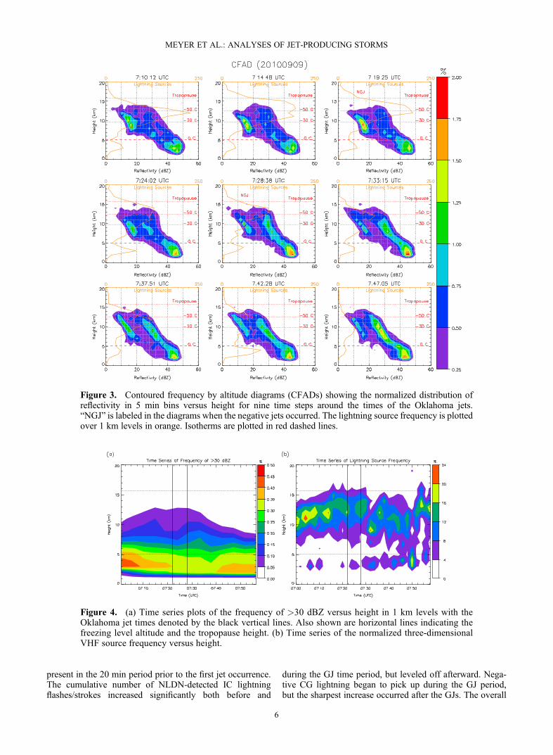
[Yuter and Houze, 1995] for the Oklahoma storm wereconstructed and overlaid with LMA altitude histograms(Figure 3). CFADs, which essentially show the probabilitydistribution of radar reflectivity as a function of altitude,are useful for detecting important changes in storm structuresuch as convective surges and overshooting tops. Thetemporal period for data integration in each Figure 3 subplotwas the duration of the radar volume scan (~4.5 min). Throughthe times of the two GJs, there was a large maximum in light-ning source frequency near the �50�C isotherm, indicatingprolific IC activity and storm intensification. There was also agreater frequency of high reflectivity values (e.g., >30 dBZ)near �50�C. This suggested a strong updraft lofting ice parti-cles to high altitudes. After the two jets, the storm weakened,indicated by a decrease in lightning sources and the reducedfrequency of significant reflectivity at middle and upperlevels. The frequency in low-level, high reflectivity valuesincreased at this point as well, indicating that large,precipitation-sized particles were falling out.[26] Time series plots of lightning and reflectivity

frequency also show the presence of a convective surge priorto the GJs. Figure 4a shows a peak of >30 dBZ frequencyjust before the first jet, which continued through the time ofthe second jet, then decreased. A time series of the VHF sourcefrequency from the LMA showed a general increase in thenumber and modal height of VHF sources above 10 km priorto the jets (Figure 4b). After the jets occurred, there was a dipin the lightning source frequency in the upper levels.[27] The NLDN time series show the storm was producing

mostly IC lightning (Figure 5). Very little CG lightning was


4

http://www.spc.ncep.noaa.gov/exper/archive/events/searchindex.html

http://www.spc.ncep.noaa.gov/exper/archive/events/searchindex.html

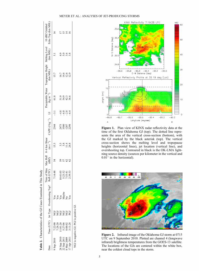
Figure 1. Plan view of KINX radar reflectivity data at thetime of the first Oklahoma GJ (top). The dotted line repre-sents the area of the vertical cross-section (bottom), withthe GJ marked by the black asterisk (top). The verticalcross-section shows the melting level and tropopauseheights (horizontal lines), jet location (vertical line), andovershooting top. Contoured in black is the OK-LMA light-ning source density (sources per kilometer in the vertical and0.01� in the horizontal).

Tab

le2.

Characteristicsof

theGJCases

Examined

inThisStudy

Date

Tim

e(U

TC)

JetType

OvershootingTop?

Tim

eof

Max

Refl

(UTC)

Max

Refl

(dBZ)

0–6km

Shear

(ms�

1)

CAPE(J

kg�1)

LI

PrecipitableWater

(kgm

�2)

TropopauseHeight

(km

MSL)

Meltin

gLevel

(km

MSL)

10dB

ZGridded

EchoTop

(km

MSL)

9Sep

2010

7:22:00

NGJ

Yes

7:14:48

5415.3

2344

�3.1

61.8

15.7

5.1

167:28:20

NGJ

Yes

28Sep

2010

11:01:20

NGJ

Yes

10:41:03

593.5

2473

�4.8

51.9

16.7

4.9

1722

Sep

2011

5:27:06

NGJ

Maybe

5:23:32

573.8

3500

�6.0

54.9

14.6

5.0

158May

2009

8:08:02

NGJ

No

7:53:41

6211.4

1207

�2.8

42.3

12.6

3.6

1417

Apr

2011

3:11:28

PGJ

Yes

2:39:33

6224.8

2298

�6.4

36.6

12.9

3.8

16

NGJisnegativ

eGJ;PGJispositiv

eGJ.

Figure 2. Infrared image of the Oklahoma GJ storm at 0715UTC on 9 September 2010. Plotted are channel 4 (longwaveinfrared) brightness temperatures from the GOES-13 satellite.The locations of the GJs are centered within the white box,near the coldest cloud tops in the storm.


5

present in the 20 min period prior to the first jet occurrence.The cumulative number of NLDN-detected IC lightningflashes/strokes increased significantly both before and

during the GJ time period, but leveled off afterward. Nega-tive CG lightning began to pick up during the GJ period,but the sharpest increase occurred after the GJs. The overall

Figure 3. Contoured frequency by altitude diagrams (CFADs) showing the normalized distribution ofreflectivity in 5 min bins versus height for nine time steps around the times of the Oklahoma jets.“NGJ” is labeled in the diagrams when the negative jets occurred. The lightning source frequency is plottedover 1 km levels in orange. Isotherms are plotted in red dashed lines.

Figure 4. (a) Time series plots of the frequency of >30 dBZ versus height in 1 km levels with theOklahoma jet times denoted by the black vertical lines. Also shown are horizontal lines indicating thefreezing level altitude and the tropopause height. (b) Time series of the normalized three-dimensionalVHF source frequency versus height.


6

results were consistent with storm intensification beginningprior to the occurrence of the GJs.

3.2. Florida

3.2.1. Overview[28] On 28 September 2010, another negative GJ was

recorded in Sebring, Florida (27.52�N, 81.52�W). A Watec902H2 camera was used to capture the jet, the same typeused in the Oklahoma case. The GJ occurred off the eastcoast of Florida at 11:01 UTC ~70 km north of the 4DLSS.Its location was fixed via query of the 4DLSS data near thetime of the GJ [Lu et al., 2011b]. This storm also was wellwithin detection range of the NLDN.3.2.2. Environment[29] The sounding (Table 2) was taken from Tampa

(KTWB) at 12 UTC, an hour after the jet occurred. Themelting level was similar to the Oklahoma case at 4.9 km.However, the tropopause was about 1 km higher at 16.7km, and the CAPE values were ~2500 J kg�1 with an LIof �4.8. Wind shear was much weaker than the Oklahomastorm, but precipitable water was over 50 kg m�2. Thisindicated a very moist, unstable air mass with tropicalcharacteristics. The GJ storm moved ~8 m s�1 toward thenorth-northeast.3.2.3. Results[30] A plan view of reflectivity data near the surface and a

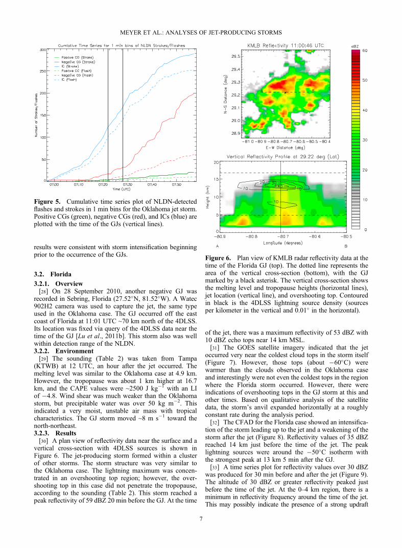
vertical cross-section with 4DLSS sources is shown inFigure 6. The jet-producing storm formed within a clusterof other storms. The storm structure was very similar tothe Oklahoma case. The lightning maximum was concen-trated in an overshooting top region; however, the over-shooting top in this case did not penetrate the tropopause,according to the sounding (Table 2). This storm reached apeak reflectivity of 59 dBZ 20 min before the GJ. At the time

of the jet, there was a maximum reflectivity of 53 dBZ with10 dBZ echo tops near 14 km MSL.[31] The GOES satellite imagery indicated that the jet

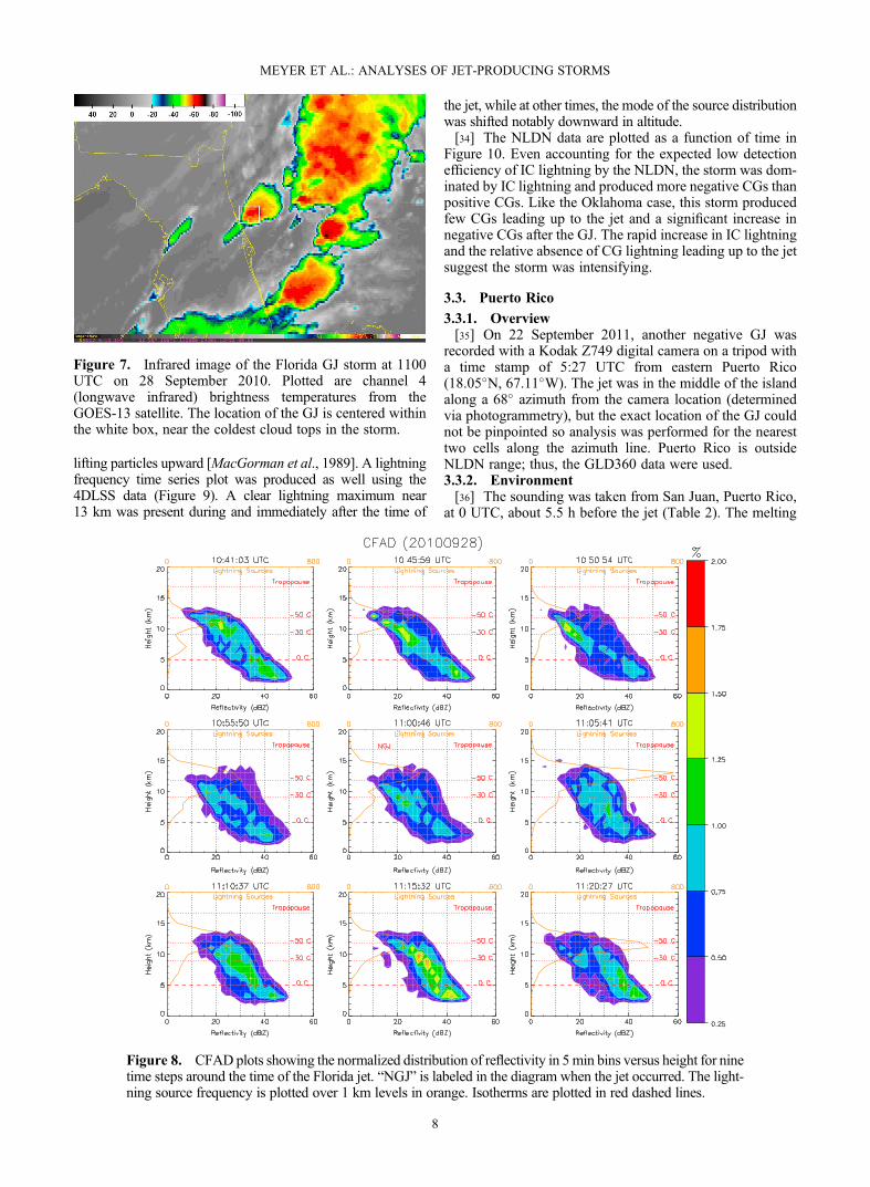
occurred very near the coldest cloud tops in the storm itself(Figure 7). However, those tops (about �60�C) werewarmer than the clouds observed in the Oklahoma caseand interestingly were not even the coldest tops in the regionwhere the Florida storm occurred. However, there wereindications of overshooting tops in the GJ storm at this andother times. Based on qualitative analysis of the satellitedata, the storm’s anvil expanded horizontally at a roughlyconstant rate during the analysis period.[32] The CFAD for the Florida case showed an intensifica-

tion of the storm leading up to the jet and a weakening of thestorm after the jet (Figure 8). Reflectivity values of 35 dBZreached 14 km just before the time of the jet. The peaklightning sources were around the �50�C isotherm withthe strongest peak at 13 km 5 min after the GJ.[33] A time series plot for reflectivity values over 30 dBZ

was produced for 30 min before and after the jet (Figure 9).The altitude of 30 dBZ or greater reflectivity peaked justbefore the time of the jet. At the 0–4 km region, there is aminimum in reflectivity frequency around the time of the jet.This may possibly indicate the presence of a strong updraft

Figure 5. Cumulative time series plot of NLDN-detectedflashes and strokes in 1 min bins for the Oklahoma jet storm.Positive CGs (green), negative CGs (red), and ICs (blue) areplotted with the time of the GJs (vertical lines).

Figure 6. Plan view of KMLB radar reflectivity data at thetime of the Florida GJ (top). The dotted line represents thearea of the vertical cross-section (bottom), with the GJmarked by a black asterisk. The vertical cross-section showsthe melting level and tropopause heights (horizontal lines),jet location (vertical line), and overshooting top. Contouredin black is the 4DLSS lightning source density (sourcesper kilometer in the vertical and 0.01� in the horizontal).


7

lifting particles upward [MacGorman et al., 1989]. A lightningfrequency time series plot was produced as well using the4DLSS data (Figure 9). A clear lightning maximum near13 km was present during and immediately after the time of

the jet, while at other times, the mode of the source distributionwas shifted notably downward in altitude.[34] The NLDN data are plotted as a function of time in

Figure 10. Even accounting for the expected low detectionefficiency of IC lightning by the NLDN, the storm was dom-inated by IC lightning and produced more negative CGs thanpositive CGs. Like the Oklahoma case, this storm producedfew CGs leading up to the jet and a significant increase innegative CGs after the GJ. The rapid increase in IC lightningand the relative absence of CG lightning leading up to the jetsuggest the storm was intensifying.

3.3. Puerto Rico

3.3.1. Overview[35] On 22 September 2011, another negative GJ was

recorded with a Kodak Z749 digital camera on a tripod witha time stamp of 5:27 UTC from eastern Puerto Rico(18.05�N, 67.11�W). The jet was in the middle of the islandalong a 68� azimuth from the camera location (determinedvia photogrammetry), but the exact location of the GJ couldnot be pinpointed so analysis was performed for the nearesttwo cells along the azimuth line. Puerto Rico is outsideNLDN range; thus, the GLD360 data were used.3.3.2. Environment[36] The sounding was taken from San Juan, Puerto Rico,

at 0 UTC, about 5.5 h before the jet (Table 2). The melting

Figure 7. Infrared image of the Florida GJ storm at 1100UTC on 28 September 2010. Plotted are channel 4(longwave infrared) brightness temperatures from theGOES-13 satellite. The location of the GJ is centered withinthe white box, near the coldest cloud tops in the storm.

Figure 8. CFAD plots showing the normalized distribution of reflectivity in 5min bins versus height for ninetime steps around the time of the Florida jet. “NGJ” is labeled in the diagram when the jet occurred. The light-ning source frequency is plotted over 1 km levels in orange. Isotherms are plotted in red dashed lines.


8

level was the same as the previous cases at 5.0 km, and thetropopause height was a little bit lower at 14.6 km. TheCAPE value was 3500 J kg�1 with an LI of �6.0. Windshear was weak, comparable to the Florida case. Precipitablewater was 54.9 kg m�2. Overall, the environment featuredtropical characteristics and was favorable for strong thunder-storms. The GJ storm moved toward the west-southwest at~14 m s�1.3.3.3. Results[37] As stated before, the specific cell that produced the

Puerto Rico jet could not be uniquely identified, and 3Dlightning mapping observations were not available for anal-ysis; however, the storm structure could still be analyzedwith radar observations. The two storms in the vicinity ofthe jet were the strongest cells in the area. A cross-sectionwas drawn through both possible cells (A and B; Figure 11),

along the approximate camera viewing azimuth, and the cellcloser to the camera appeared to have a small overshootingtop similar to the other cases. The storm farther from thecamera did not have an overshooting top. The maximumreflectivity was 57 dBZ 5 min prior to the jet, with an echotop height of 15 km MSL, again similar to the Oklahomaand Florida cases. The ambiguity in position precludeddirectly associating the jet with the coldest cloud tops in

Figure 9. (a) Time series plots of the frequency of >30 dBZ versus height in 1 km levels with theFlorida jet time denoted by the black vertical line. Also shown are horizontal lines indicating thefreezing level altitude and the tropopause height. (b) Time series of the normalized three-dimensionalVHF source frequency versus height.

Figure 10. Cumulative time series plot for NLDN-detectedflashes and strokes in 1 min bins. Positive CGs (green), neg-ative CGs (red), and ICs (blue) are plotted with the time ofthe GJ (vertical line).

Figure 11. Plan view of TJUA radar reflectivity data at thetime of the Puerto Rico GJ (top). The dotted line representsthe area of the vertical cross-section (bottom). The verticalcross-section shows the melting level and tropopauseheights (horizontal lines).


9

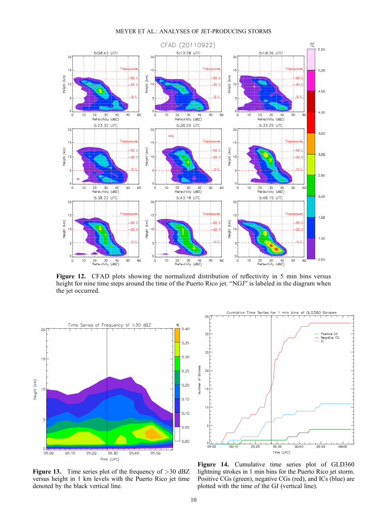
Figure 12. CFAD plots showing the normalized distribution of reflectivity in 5 min bins versusheight for nine time steps around the time of the Puerto Rico jet. “NGJ” is labeled in the diagram whenthe jet occurred.

Figure 13. Time series plot of the frequency of >30 dBZversus height in 1 km levels with the Puerto Rico jet timedenoted by the black vertical line.

Figure 14. Cumulative time series plot of GLD360lightning strokes in 1 min bins for the Puerto Rico jet storm.Positive CGs (green), negative CGs (red), and ICs (blue) areplotted with the time of the GJ (vertical line).


10

the storm. However, infrared satellite imagery (not shown)showed that the storm featured cloud-top brightness tem-peratures near�65�C. Around the time of the GJ, the stormwas undergoing a broad minimum in cloud-top temperaturewith possible indications of overshooting tops. Based onqualitative analysis of the satellite data, the storm’s anvilexpanded horizontally at a roughly constant rate duringthe analysis period.[38] Like the previous cases, CFADs were produced; how-

ever, only reflectivity frequency was plotted since 3D light-ning data were unavailable (Figure 12). Reflectivity data forboth possible cells were included in the analysis since theywere less than 5 km apart. An increase in 20–30 dBZfrequencies pushed through the tropopause height leadingup to the time of the jet. The 5 min period after the jetoccurred featured the peak frequency of 25 dBZ in the upperlevels, indicating the storm was at its peak intensity. Thenext few scans showed that the maximum in the upper levelreflectivity values started to shrink, and the frequency of the30 dBZ increased near the lower levels, suggesting the largerhydrometeors were falling out.[39] The time series reflectivity plot was consistent with

the CFADs (Figure 13). A broad peak height of >30 dBZfrequencies occurred during and after the time of the jet.Similar to the Oklahoma and Florida cases, there was a min-imum frequency of>30 dBZ in the lower layers, suggesting

the particles were being lifted by a strong updraft aroundthis time.[40] Figure 14 shows a limited number of strokes detected

by the GLD360. This was due in part to a lower flash detec-tion efficiency and larger uncertainty in location accuracythan NLDN [Demetriades et al., 2010]. Overall, the stormwas �CG dominant with an increase in strokes before andduring the time of the jet, in contrast to the Oklahomaand Florida cases. Flash data were not available, however,and it is possible that a small number of high-multiplicitynegative CG flashes accounted for the increase in cumulativestroke rate.

3.4. North Carolina

3.4.1. Overview[41] Two GJs have been recorded off the coast of North

Carolina since 2009, one being negative and another beingpositive. The negative jet was recorded on 8 May 2009 at8:08 UTC. The positive jet was observed on 17 April 2011at 3:11 UTC. Both of these GJs were recorded by a WATEC902H2 camera coupled to a triggered video acquisition sys-tem that records approximately 1 s of video when specifiedcriteria are met. This camera is located in a field near DukeUniversity (35.975�N, 79.100�W) [Cummer et al., 2009].The exact position of the negative GJ could not bepinpointed, but it was seen along a 117�–118� azimuth from

Figure 15. Plan view of KMHX radar reflectivity data atthe time of the North Carolina negative GJ (top). The dottedline represents the area of the vertical cross-section (bottom).The vertical cross-section shows the melting level and tropo-pause heights (horizontal lines).

Figure 16. Plan view of KMHX radar reflectivity data at thetime of the North Carolina positive GJ (top). The dotted line rep-resents the area of the vertical cross-section (bottom), along theazimuth of the observed GJ. The vertical cross-section showsthe melting level and tropopause heights (horizontal lines).


11

the camera (determined via photogrammetry). The positiveGJ occurred along an azimuth of 125�–126� from the camera(determined via photogrammetry), in a squall line off the

coast of North Carolina [Lu et al., 2011a]. Based on anaverage position of a group of negative CGs that occurredapproximately 1 s before the positive GJ, its likely positionwas somewhere near 34.23�N, 76.21�W. Like the PuertoRico case, there were no VHF lightning mapping networksin the area; however, both of these GJ-producing stormswere within NLDN range. The KMHX radar in Morehead,North Carolina, was used to analyze the reflectivity data.3.4.2. Environment[42] The soundings for both North Carolina cases were taken

fromMorehead City, North Carolina (Table 2). The 2009 neg-ative GJ sounding at 0 UTC on 8 May showed melting leveland tropopause heights at 3.6 and 12.6 km, respectively. Thiswas lower than the other GJ cases, likely due to the springtimeoccurrence of the storm. The CAPE value was ~1200 J kg�1,and the LI was �2.8. Wind shear was over 10 m s�1, whileprecipitable water also was 42.3 kg m�2. The atmospherewas thus drier and more stable than the other cases, though itwas still typical of tropical environments [Zveryaev and Chu,2003]. The 12 UTC sounding from this day was even drierand more stable than the 0 UTC one; however, the later sound-ing was affected by the passage of the storm as it movedoffshore, toward the east at ~20 m s�1.[43] The 2011 positive GJ case sounding at 0 UTC on 17

April had a melting level and tropopause height of 3.8 and

Figure 17. Infrared image of the North Carolina positive GJstorm at 0315 UTC on 11 April 2011. Plotted are channel 4(longwave infrared) brightness temperatures from the GOES-13 satellite. The most likely location of the GJ is within thewhite box, near the coldest cloud tops in the storm.

Figure 18. CFAD plots showing the normalized distribution of reflectivity in 5 min bins versus heightfor nine time steps around the time of the negative North Carolina jet. “NGJ” is labeled in the diagramwhen the jet occurred.


12

12.9 km, respectively. CAPE value was ~2300 J kg�1, andLI was�6.4. Precipitable water was 36.6 kg m�2, the lowestof all cases but still typical of the tropics [Zveryaev and Chu,2003]. Meanwhile, wind shear was strongest of all the cases:~25 m s�1. The storm itself moved ~20 m s�1 toward theeast. In summary, the soundings from both of these dayssuggested favorable environments for thunderstorm forma-tion, and the atmosphere was very moist, reminiscent oftropical air masses.3.4.3. Results[44] The storm from which the negative GJ initiated was

an isolated storm, the largest in the immediate area(Figure 15). Thus, despite the ambiguity in jet position, itwas clear that this storm had produced it. The 2009 negativeGJ cell was about 110 km away from the KMHX radar. Thevertical cross-section along the camera azimuth does notshow an obvious overshooting top for this case, although thereis a broad region of elevated echo tops along the 20–28 kmrange interval (Figure 15). The maximum reflectivity in thisstorm was 62 dBZ about 15 min before the jet. The 10 dBZcontour reached 14 km MSL, but this occurred ~30 min priorto the GJ. Storm echo tops were about 2 km lower at the timeof the jet, as can be seen in Figure 15. Similar to the Puerto Ricocase, the location uncertainty does not allow the ability to ascer-tain the exact proximity of the jet relative to the coldest cloudtops. However, the infrared satellite imagery (not shown)showed that the minimum cloud top temperatures werenear �60�C. The most likely time of occurrence for

overshooting tops, based on interpretation of the satellitedata, was 30–45 min prior to the GJ. Based on qualitativeanalysis of the satellite data, the storm’s anvil expanded hori-zontally at a roughly constant rate during the analysis period.[45] The 2011 positive GJ storm is shown in Figure 16.

The positive jet originated from a squall line moving offthe coast. The storm was about 90 km from the KMHXradar. There was a small region of 15–20 dBZ above thelocal tropopause which indicated an overshooting top alongthe azimuth of the jet. This storm had a peak reflectivityvalue of 62 dBZ with 10 dBZ echo tops at 16 km MSL.Based on its azimuth and the location of CG activity imme-diately beforehand, the jet likely occurred very near thecoldest IR cloud-top temperatures in the storm, which wereapproximately �70�C (Figure 17). Note the V-shapedstructure in the cold cloud of this storm, which encom-passes a warmer interior east of it. U-shapes, V-shapes,and rings in cold cloud structure sometimes occur in stormsproducing overshooting tops, with the V-shape more likelywhen wind shear is strong [Setvak et al., 2010]. Based onqualitative analysis of the satellite data, the storm’s anvilexpanded horizontally at a roughly constant rate duringthe analysis period.[46] Since there are no LMA networks in North Carolina,

3D lightning analysis was not possible. The CFAD plots forthe negative jet showed different results compared to theprevious cases (Figure 18). There was a small maximum infrequency of 35 dBZ values present between the �30�C

Figure 19. CFAD plots showing the normalized distribution of reflectivity in 5 min bins versus heightfor nine time steps around the time of the North Carolina positive jet. “PGJ” is labeled in the diagramwhen the jet occurred.


13

and �50�C isotherms in the first frame, but this decreasedleading up to the time of the jet, suggesting the storm wasweakening. However, the frequency of 10–20 dBZ valuesin the upper levels continued to increase throughout thewhole time period, possibly suggesting a broadening anvil.The CFADs in the positive jet case more closely resembledthose in the previous cases (Figure 19). A maximum infrequency of 30–40 dBZ values at high altitudes becamemore prominent leading up to the time of the jet. By thetime of the last frame, the maximum frequency was in thelower 5 km, indicating that the storm was raining out andweakening.[47] A time series of reflectivity for the 2009 negative GJ

case is consistent with the CFADs (Figure 20a). Unlike allthe other cases, the reflectivity frequency in the upper levelswas at a minimum near the time of the jet. There was also aminimum in low-level reflectivity frequency around the timeof the jet which was similar to the previous cases. The timeseries reflectivity for the 2011 positive GJ case shows a fairlyflat maximum height for 30 dBZ echo or greater, except for asmall peak within the 5 min period after the jet (Figure 20b).However, reflectivity frequencies at lower altitudes were more

dynamic, with the jet occurring between two surges infrequency of 30+ dBZ below about 7 km MSL.[48] The NLDN time series for the North Carolina cases

are shown in Figure 21. Only flash data were accessible forthis case. The majority of the flashes were negative CGs,and overall, very little NLDN-detected IC and positive CGlightning was noted. The 2009 negative GJ case had a lullin all lightning leading up to the time of the jet and thenthe negative CG lightning picked up afterward (Figure 21a).This negative CG pattern is similar to that of the Oklahomaand Florida cases. The positive jet case had a lot of negativeCG activity in the beginning of the analysis, which thenleveled off through the time of jet occurrence (Figure 21b).

4. Conclusions

[49] The radar and lightning characteristics of five differ-ent thunderstorms that produced a total of six GJs have beenexamined. Table 2 shows a summary of these cases alongwith some of their storm characteristics. Three of them werenear VHF lightning mapping networks. The Oklahoma caseformed in remnants of Tropical Storm Hermine, with typical

Figure 20. Time series plots of the frequency of >30 dBZ versus height in 1 km levels with the jet timedenoted by the black vertical line for (a) 8 May 2009 (negative GJ) and (b) 17 April 2011 (positive GJ).

Figure 21. (a) Cumulative time series plot of NLDN lightning flashes in 1 min bins for the negativeNorth Carolina jet storm. Positive CGs (green), negative CGs (red), and ICs (blue) are plotted with thetime of the GJ (vertical line). (b) Same as (a) but for the positive North Carolina jet storm.


14

tropical cyclone environmental characteristics such as highamounts of moisture. The Florida, Puerto Rico, and NorthCarolina storms formed in moist environments with highCAPE and negative LI values. The Oklahoma and PuertoRico GJs were located over land, and the Florida and NorthCarolina cases occurred over water. No obvious or system-atic land/water differences between the cases were apparentin environmental parameters or storm characteristics. Bycomparison, the multi-GJ storm studied by Soula et al.[2011] also developed in a very moist environment withelevated CAPE.[50] The maximum reflectivity in the observed cases

ranged from 54 to 62 dBZ, with 10 dBZ echo tops greaterthan 14 km MSL in all storms. Five out of the six cases fea-tured what appeared to be overshooting tops in the radar dataaround the time of the jets, whether those tops broke throughthe sounding-defined tropopause. Temporal behavior ofreflectivity in five of the six cases supported the notion ofstorms being near peak reflectivity height and/or verticalintensity around the times of the jets, indicating the stormswere undergoing or had just passed the peak of a convectivesurge. Infrared satellite data, when the locations of GJs couldbe pinpointed, showed the GJs as occurring near thecoldest cloud tops, though cloud-top temperature varied sub-stantially between the different storms. By comparison, theGJ-producing storm studied by van der Velde et al., 2007afeatured 40 dBZ echoes as high as 12–15 km, with echo topsup to 17–20 km. Thus, the storms in the present study,though tall and intense, are not the tallest or strongest stormsto have produced a GJ.[51] The Oklahoma and Florida cases were marked by

frequent high-altitude lightning as determined by VHFmapping networks, leading up to the time of the jets. Thelightning decreased afterwards. All storms produced morenegative than positive CG lightning during the 1 h analysistimes that encompassed the jets. Sometimes negative CGlightning mainly occurred prior to the jets (North Carolinapositive GJ), and sometimes it mainly increased afterward(Oklahoma, Florida, North Carolina negative GJ). In thePuerto Rico case, negative CGs were produced inthe greatest numbers around the time of the GJ, althoughthe overall number of strokes was small. The Puerto Rico re-sult is most similar to the observations of Soula et al. [2011],who found rapid changes in lightning flash rate to occurduring the GJ-producing times of one thunderstorm. Regard-less, the negative CG dominance, as well as the presence ofupper level VHF source maxima when those observationswere available, indicates that most likely all the jet-producing storms were normal polarity [Lang and Rutledge,2011]. This was confirmed by Lu et al. [2011b] for theOklahoma and Florida storms via more detailed flash analysis.[52] The observations suggest a potential link between

convective surges and the occurrence of gigantic jets.Riousset et al. [2010] offered a physical mechanism forwhy this might be the case. Using a simplified model, theyfound that strong mixing of upper positive charge andnegative screening charge could lead to electrodynamic con-ditions favoring the generation of a GJ. Riousset et al.[2010] suggested that such mixing could occur near over-shooting tops or other areas of strong turbulence in the upperlevels of a cloud. The present observations tend to supportRiousset et al. [2010], since convective surges and

overshooting tops were so closely associated with the oc-currence of most GJs. However, some caution needs to beexercised, for a couple reasons. The first is that very littleis understood about the behavior of thundercloud chargeregions in the turbulent upper levels of a convectivelysurging thunderstorm, and the relative roles of turbulentmixing, advective displacement, in situ charging, frequentlightning, and other processes—in either depleting orenhancing regions of net charge—are not well quantified.Modeling studies like Krehbiel et al. [2008] and Rioussetet al. [2010] provide a useful framework for interpretingthe present observational results, but they do not providethe last word on the matter.[53] The second caveat is the case of the negative North

Carolina jet, which occurred as the strongest reflectivitiesdecreased in altitude and the storm weakened, and occurredmore than 20 min past the time of peak vertical develop-ment. This was not consistent with the other cases, and thus,gigantic jets are not exclusive to times near the peak of aconvective surge. Without 3D lightning information, it isdifficult to say with any certainty what was truly differentabout this particular case. Future modeling efforts will needto account for the ability of GJs to occur under different cir-cumstances than just convective surges.[54] One interesting observation is the North Carolina

storm that produced the positive GJ. This storm appearedto be normal polarity. Krehbiel et al. [2008] suggested thatinverted storms, with positive charge in middle levels,would be the likely producers of positive GJs, and notnormal polarity thunderstorms. There are a couple possibleexplanations for this unexpected behavior. One is that thethunderstorm was undergoing an overall rapid decline innegative CG rate through the time of the jet, with �CG ratesthen less than a third of what they were 30 min earlier. Thisobservation was similar to van der Velde et al. [2007a] andmay have indicated that a major shift in thunderstorm chargestructure was occurring, one that potentially may havefavored the production of a positive GJ. The second possibil-ity is that this was a Type II gigantic jet as described byChou et al. [2010] and thus originated as a blue jet (i.e., positiveleader) between the upper positive charge and negative screen-ing layer. Clearly, both of these hypotheses would requiremoredetailed lightning and charge observations to test. Oneadditional note is that the positive GJ observed by van derVelde et al. [2010] occurred in environment of strong windshear, similar to the present case.[55] The meteorological regimes examined here

(multicellular tropical or tropical-like convective storms)are distinctly different from those associated with mostsprite-producing convective systems [Lyons, 2006; Lyonset al., 2009]. However, these are not the only meteorologicalregimes in which GJs occur. For example, van der Veldeet al. [2010] studied a GJ that occurred over relativelyshallow wintertime convection. Clearly, many additionalcase studies of GJ-producing storms are required to resolvethe ambiguities observed in this study, and to more accu-rately characterize the range of meteorological scenarios inwhich gigantic jets occur. In addition, a major questionremains about the relative rarity of GJs compared to thefrequency of convective surges and overshooting tops.This would require extensive analysis of null cases (i.e.,storms with unobstructed camera observations but no GJ


15

production) to answer, suggesting a fruitful avenue forfuture GJ research.

[56] Acknowledgments. This work was supported by the DARPANimbus program. The authors thank Vaisala, Inc. for providing the NLDNand GLD360 data used in this study. Without the observations of the gigan-tic jets, this study would not have been possible. The Florida, Oklahoma,and Puerto Rico gigantic jets were observed by Joel Gonzalez in Florida,by Kevin Palivec in Texas, and by Frankie Lucena in Puerto Rico, respec-tively. The authors thank the editors and reviewers of this manuscript fortheir assistance in improving it.

ReferencesBiagi, C. J., K. L. Cummins, K. E. Kehoe, and E. P. Krider (2007), NationalLightning Detection Network (NLDN) performance in southern Arizona,Texas, and Oklahoma in 2003–2004. J. Geophys. Res., 112, doi:10.1029/2006JD007341.

Boyd, B. F., W. P. Roeder, D. Hajek, and M. B. Wilson (2005), Installation,upgrade, and evaluation a short baseline cloud-to-ground lightning sur-veillance system in support of space launch operations, 1st Conferenceon Meteorological Applications of Lightning Data, 9–13, Jan 05, 4 pp.

Chou, J. K., et al. (2010), Gigantic jets with negative and positive polaritystreamers, J. Geophys. Res., 115, A00E45, doi:10.1029/2009JA014831.

Chou, J. K., L. Y. Tsai, C. L. Kuo, Y. J. Lee, C. M. Chen, A. B. Chen, H. T.Su, R. R. Hsu, P. L. Chang, and L. C. Lee (2011), Optical emissions andbehaviors of the blue starters, blue jets, and gigantic jets observed in theTaiwan transient luminous event ground campaign, J. Geophys. Res.,116, A07301, doi:10.1029/2010JA016162.

Cummer, S. A., et al. (2009), Quantification of the troposphere to iono-sphere charge transfer in a gigantic jet, Nat. Geosci., 2, 617–620,doi:10.1038/ngeo607.

Cummins, K. L., Krider, E. P., Malone, M. D. (1998), The U.S. national light-ning detection network and applications of cloud-to-ground lightning data byelectric power utilities. IEEE Trans. Electromagn. Compat., 40(4), 465–480.

Cummins, K. L., and M. J. Murphy (2009), An overview of lightning loca-tion systems: History, techniques, and data uses, with an in-depth look atthe U.S. NLDN, IEEE Trans. Electromagn. Compat., 51(3), 499–518.

Demetriades, N. W. S., M. J. Murphy, and J. A. Cramer (2010), Validationof Vaisala’s Global Lightning Dataset (GLD360) over the continentalUnited States. Preprints, 29th Conf. Hurricanes and Tropical Meteorol-ogy, May 10–14, Tucson, AZ, 6 pp.

Holle, R. (2009), http://www.srh.noaa.gov/media/abq/sswhm/Holle_sw_hydromet_09.pdf.

Hondl, K. D., (2003), Capabilities and components of the Warning DecisionSupport System-Integrated Information (WDSS-II), Preprints, 19th Conf.on Interactive Information Processing Systems (IIPS) for Meteorology,Oceanography, and Hydrology, Long Beach, CA, Amer. Meteor. Soc.,CD-ROM, 14.7.

Hsu, R., et al. (2004), Transient luminous jets recorded in the Taiwan 2004TLE campaign, Eos Trans. AGU, 85(47), Fall Meet. Suppl., AbstractAW31a-0151.

Krehbiel, P. R., J. A. Riousset, V. P. Pasko, R. J. Thomas, W. Rison, M. A.Stanley, and H. E. Edens (2008), Upward electrical discharges fromthunderstorms, Nat. Geosci., 1, 233–237, dio:10.1038/ngeo162.

Krehbiel, P. R., R. J. Thomas, W. Rison, T. Hamlin, J. Harlin, and M. Davis(2000), GPS-based mapping system reveals lightning inside storms, EosTrans. AGU, 81(3), 21–21, 10.1029/00EO00014.

Lang, T. J., J. Li, W. A. Lyons, S. A. Cummer, S. A. Rutledge, and D. R.MacGorman (2011), Transient luminous events above two mesoscaleconvective systems: Charge moment change analysis, J. Geophys. Res.,116, A10306, doi:10.1029/2011JA016758.

Lang, T. J., W. A. Lyons, S. A. Rutledge, J. D. Meyer, D. R. MacGorman,and S. A. Cummer (2010), Transient luminous events above two meso-scale convective systems: Storm structure and evolution, J. Geophys.Res., 115, A00E22, doi:10.1029/2009JA014500.

Lang, T. J., S. A. Rutledge 2011, A framework for the statistical analysis oflarge radar and lightning datasets: Results from STEPS 2000, Mon. Wea.Rev., 139, 2536–2551.

Lakshmanan, V., T. Smith, K. Hondl, G. J. Stumpf, and A. Witt (2006), Areal-time, three dimensional, rapidly updating, heterogeneous radarmerger technique for reflectivity, velocity, and derived products, Wea.Forecasting, 21 (5), 802–823.

Lakshmanan, V., T. Smith, G. Stumpf, and K. Hondl. (2007), The WarningDecision Support System-Integrated Information, Wea. And Forecasting,22, 596–612.

Lennon, C. and L. Maier, (1991), Lightning mapping system. 1991 Int’l.Aerospace and Ground Conf. on Lightning and Static Elec., NASA Conf.Pub. 3106, paper 89-1.

Lu, G. et al. (2011a), Analysis of lightning development associated withgigantic jets, American Geophysics Union (AGU) Fall Meeting Abstracts,AE13B-02, 2011 December, San Francisco, United States.

Lu, G., et al. (2011b), Lightning development associated with two negativegigantic jets, Geophys. Res. Lett., 38, L12801, doi: 10.1029/2011GL047662.

Lu, G., S. A. Cummer, R. J. Blakeslee, S. Weiss, and W. H. Beasley (2012),Lightning morphology and impulse charge moment change of high peakcurrent negative strokes, J. Geophys. Res., 117, D04212, doi:10.1029/2011JD016890.

Lyons, W. A. (2006), The meteorology of transient luminous events—Anintroduction and overview, in NATO Advanced Study Institute onSprites, Elves and Intense Lightning Discharges, edited by M. Fullekruget al., pp. 19–56, Springer, New York.

Lyons, W. A., T. E. Nelson, R. A. Armstrong, V. P. Pasko, and M. A. Stanley(2003), Upward electrical discharges from the tops of thunderstorms, Bull.Amer. Meteor. Soc., 84, 445–454.

Lyons, W. A., M. A. Stanley, J. D. Meyer, T. E. Nelson, S. A. Rutledge, T. L.Lang, and S. A. Cummer 2009, The meteorological and electrical structure ofTLE-producing convective storms, in Lightning: Principles, Instruments andApplications, H. D. Betz et al. (eds), pp 389–417, Springer Science +Busi-ness Media B.V., doi: 10.1007/978-1-4020-9079-017.

MacGorman, D. R., D. W. Burgess, V. Mazur, W. D. Rust, W. L. Taylor,and B. C. Johnson 1989, Lightning rates relative to tornadic storm evolu-tion on 22 May 1981, J. Atmos. Sci., 46, 221–250.

MacGorman, D. R., et al. (2008), TELEX: The thunderstorm electrificationand lightning experiment, Bull. Am. Meteorol. Soc., 89, 997–1013,doi:10.1175/2007BAMS2352.1.

MacGorman, D. R., and K. E. Nielsen (1991), Cloud-to-ground lightning ina tornadic storm on 8 May 1986, Mon. Wea. Rev., 119, 1557–1574.

Maier, L., C. Lennon, T. Britt, and S. Schaefer (1995), LDAR systemperformance and analysis, International Conference on Cloud Physics,Amer. Meteorol. Soc., Dallas, TX.

Marshall, T. C., et al. (2005), Observed electric fields associated withlightning initiation, Geophys. Res. Lett. 32, L03813.

Mohr, C. G., and R. L. Vaughn (1979), An economical approach forCartesian interpolation and display of reflectivity factor data in three-dimensional space, J. Appl. Meteor., 18, 661–670.

Murphy, M. J., K. L. Cummins, N. W. S. Demetriades, and W. P. Roeder(2008), Performance of the new Four-Dimensional Lightning Surveil-lance System (4DLSS) at the Kennedy Space Center/Cape CanaveralAir Force Station Complex, 13th Conference on Aviation, Range, andAerospace Meteorology, Amer. Meteorol. Soc., Boston, MA.

Orville, R. E. (2008), Development of the National Lightning DetectionNetwork, Bull. Amer. Meteorol. Soc., 89(2), 180.

Pasko, V. P., and J. J. George (2002), Three-dimensional modeling of bluejets and blue starters, J. Geophys. Res., 107(A12), 1458, doi:10.1029/2002JA009473.

Pasko, V. P., M. A. Stanley, J. D. Mathews, U. S. Inan, and T. G. Wood(2002), Electrical discharge from a thundercloud top to the lower iono-sphere, Nature, 416, 152–154, doi:10.1038/416152a.

Riousset, J. A., V. P. Pasko, P. R. Krehbiel,W. Rison, andM. A. Stanley (2010),Modeling of thundercloud screening charges: Implications for blue and gigan-tic jets, J. Geophys. Res., 115, A00E10, doi:10.1029/2009JA014286.

Rison, W., R. J. Thomas, P. R. Krehbiel, T. Hamlin, and J. Harlin (1999), AGPS-based three-dimensional lightning mapping system: Initial observa-tions in central New Mexico, Geophys. Res. Lett., 26(23), 3573–3576.

Roeder, W. P. (2010), The four dimensional lightning surveillance system,21st International Lightning Detection Conference, Vaisala, Orlando, Fla.

Said, R. K., U. S. Inan, and K. L. Cummins (2010), Long-range lightninggeo-location using a VLF radio atmospheric waveform bank, J. Geophys.Res., 115, D23108, doi:10.1029/2010JD013863.

Setvak, M. et al. (2010), Satellite-observed cold-ring-shaped features atopdeep convective clouds. Atmos. Res., 97, 80–96.

Soula, S., O. van der Velde, J. Montanya, P. Huet, C. Barthe, and J. Bór (2011),Gigantic jets produced by an isolated tropical thunderstorm near RéunionIsland, J. Geophys. Res., 116, D19103, doi:10.1029/2010JD015581.

Su, H. T., et al. (2003), Gigantic jets between a thundercloud and the iono-sphere, Nature, 423, 974–976, doi:10.1038/nature01759.

van der Velde, O. A., J. Bor, J. Li, S. A. Cummer, E. Arnone, F. Zanotti, M.Fullekrug, C. Haldoupis, S. NaitAmor, and T. Farges (2010), Multi-instrumental observations of a positive gigantic jet produced by a winterthunderstorm in Europe, J. Geophys. Res., 115, D24301, doi:10.1029/2010JD014442.

van der Velde, O. A., et al. (2007a), Analysis of the first gigantic jetrecorded over continental North America, J. Geophys. Res., 112,D20104, doi:10.1029/2007JD008575.

van der Velde, O. A., W. A. Lyons, S. A. Cummer, N. Jaugey, D. D.Sentman, M. B. Cohen, and R. Smedley (2007b), Electromagnetic, visualand meteorological analyses of two gigantic jets observed over Missouri.Eos Trans AGU, Fall Meet, Suppl., Poster, Abstract AE23A-0895.


16

http://www.srh.noaa.gov/media/abq/sswhm/Holle_sw_hydromet_09.pdf

http://www.srh.noaa.gov/media/abq/sswhm/Holle_sw_hydromet_09.pdf

Wiens, K. C., Rutledge, S. A., and Tessendorf, S. A. (2005), The 29 June2000 supercell observed during STEPS. Part II: Lightning and chargestructure, J. Atmos. Sci., 62, 4151–4177.

Wescott, E. M., Stenbaek-Nielsen, H. C., Huet, P., Heavner, M. J., andMoudry, D. R. (2001), New evidence for the brightness and ionizationof blue jets and blue starters, J. Geophys. Res., 106, 21549–21554.

Wescott, E. M., Sentman, D. D., Heavner, M. J., Hampton, D. L., and O. H.Vaughan Jr. (1998), Blue jets: Their relationship to lightning and verylarge hailfall, and their physical mechanisms for their production, J.Atmos. Sol. Terr. Phys., 60, 713–724.

Williams, E. R., et al. (1999), The behavior of total lightning activity insevere Florida thunderstorms, Atmos. Res., 51, 245–264.

Wilson, C. T. R. (1956), A theory of thundercloud electricity, Proc. R. Soc.Lond., A236, 297–317.

Wilson, C. T. R. (1921), Investigations on lightning discharges andon the electric field of thunderstorms, Phil. Trans. R. Soc. Lond.,A221, 73–115.

Yuter, S. E., and R. A. Houze Jr. (1995), Three-dimensional kinematic andmicrophysical evolution of Florida cumulonimbus. Part II: Frequencydistribution of vertical velocity, reflectivity, and differential reflectivity,Mon. Wea. Rev., 123, 1941–1963.

Zveryaev, I. I. and P.-S. Chu (2003), Recent climate changes in pre-cipitable water in the global tropics as revealed in National Centersfor Environmental Prediction/National Center for AtmosphericResearch reanalysis, J. Geophys. Res.,108(D10), 4311, doi:10.1029/2002JD002476.


17

Documents

Radar and lightning analyses of gigantic jet-producing stormspeople.ee.duke.edu/~cummer/reprints/154_Meyer13_JGR_JetProducing... · Radar and lightning analyses of gigantic jet-producing