Embed Size (px)
Citation preview

International Journal of Statistics and Probability; Vol. 10, No. 3; May 2021
ISSN 1927-7032 E-ISSN 1927-7040
Published by Canadian Center of Science and Education
69
R-squared of a Latent Interaction in Structural Equation Model:
A Tutorial of Using R
Lu Qin¹, Jihong Zhang², Xinya Liang³, and Qianqian Pan⁴
¹ Department of Psychology, Howard University
² Department of Educational Measurement and Statistics, University of Iowa
³ Department of Educational Statistics & Research Method, University of Arkansas
⁴ Faculty of Education, The University of Hong Kong
Correspondence: Lu Qin, Howard University, Minor Hall 111, 2400 6th St NW, Washington DC, 20059
Received: March 4, 2021 Accepted: April 9, 2021 Online Published: April 13, 2021
doi:10.5539/ijsp.v10n3p69 URL: https://doi.org/10.5539/ijsp.v10n3p69
Abstract
Mplus (Muthén & Muthén, 1998 - 2017) is one popular statistical software to estimate the latent interaction effects
using the latent moderated structural equation approach (LMS). However, the variance explained by a latent interaction
that supports the interpretation of estimation results is not currently available from the Mplus output. To relieve human
computations and to facilitate interpretations of latent interaction effects in social science research, we developed two
functions (LIR & LOIR) in the R package IRmplus to calculate the 𝑅-squared of a latent interaction above and beyond the
first-order simple main effects in Structural Equation Modeling. This tutorial provides a step-by-step guide for applied
researchers to estimating a latent interaction effect in Mplus, and to obtaining the 𝑅-squared of a latent interaction
effect using the LIR & LOIR functions. Example data and syntax are available online.
Keywords: 𝑅-squared, latent interactions, R package, IRmplus, Mplus
Mplus (Muthén & Muthén, 1998 - 2017) is one popular statistical software for estimating various latent variable models
(Hallquist & Wiley, 2018). It has a built-in function to estimate latent interaction effects using the latent moderated
structural equation approach (LMS; Klein & Moosbrugger, 2000; Muthen & Muthen, 1998-2017). Comparing to the
product indicator approach that models the latent interactions using the products of observed indicators of exogenous
latent factors (Kenny & Judd, 1984), the LMS approach estimates the latent interactions by approximating a mixture of
conditional distributions of observed indicators (Kelava et al., 2011). When latent factors and observed indicators are
multivariate normally distributed, the LMS approach provides unbiased estimates of latent interaction effects (Kelava &
Nagengast, 2012; Cham, West, Ma, & Aiken, 2012). However, this approach is limited in that the Mplus output does not
provide model fit measures, 𝑅-squared estimation, or standardized parameter estimates. Obtaining these quantities
requires to run additional analyses or use hand computations. For example, the model fit comparison by the
log-likelihood ratio test (LRT; Neyman & Pearson, 1933) can be conducted using the function compareModels in the R
package MplusAutomation (Hallquist & Wiley, 2018). To obtain standardized parameter estimates, one may first
standardize all variables in the dataset, and then perform an analysis in Mplus based on the standardized variables
(Maslowsky, Jager, & Hemken, 2015). Nonetheless, for the 𝑅-squared of latent interactions, manual computations are
necessary, although equations of the 𝑅-squared estimation have been presented in Maslowsky and Hemken (2015).
Using and reporting the 𝑅-squared of latent interaction effects remains a challenge for applied researchers due to the
computational complexity.
To relieve human computations and to facilitate interpretations of latent interaction effects in practice, we developed
two functions (LIR and LOIR) in an R package IRmplus to calculate the variance explained by the latent interaction above
and beyond the first-order simple main effects in latent variable modeling. R is a leading programming software that
supports data analysis and statistical modeling (R Core Team, 2017), which has been widely used in social science
studies.
In this paper, we briefly introduce the computation of the 𝑅-squared of a latent interaction and the IRmplus package,
followed by two examples using the LIR and LOIR functions in the IRmplus package. The strengths and limitations are
discussed at the end.
http://ijsp.ccsenet.org International Journal of Statistics and Probability Vol. 10, No. 3; 2021
70
A Brief Overview of the 𝐑-squared of Latent Interaction
Interactions between two latent variables are often estimated in structural equation models (SEM). SEM allows for
testing a variety of hypothesized models to explain the relationships among a set of latent factors and observed variables
(e.g., Bollen, 1989; Ullman & Bentler, 2003). SEM is composed of a measurement model and a structural model
(Schumacker & Lomax, 2004). The measurement model examines the associations between latent factors and observed
indicators. Let 𝑖 be an 𝑖𝑡ℎ individual, 𝑝 be a number of observed indicators, and 𝑚 be a number of latent factors.
The measurement model is expressed in Equation (1) as:
𝐲i = 𝛎 + 𝚲𝛚𝑖 + 𝛆i (1)
where 𝐲i is a 𝑝 × 1 vector of observed indicators, 𝛎 is a 𝑝 × 1vector of intercepts, 𝚲 is a 𝑝 × 𝑚 matrix of factor
loadings, 𝛚i is a 𝑚 × 1 vector of latent factors, and 𝛆i is a 𝑝 × 1 vector of measurement errors that assumes a
multivariate normal distribution with a mean vector of 𝟎 and a diagonal matrix of 𝚿.
The structural model explains the relationships among latent factors or among latent factors and observed covariates.
The two-way latent interactions can be estimated in the structural model under two scenarios: (1) between latent factors,
and (2) between a latent factor and an observed covariate, detailed in the following scenarios.
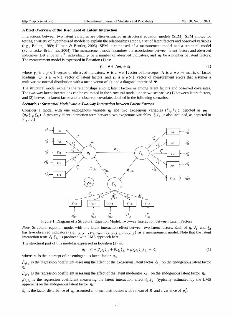
Scenario 1: Structural Model with a Two-way Interaction between Latent Factors
Consider a model with one endogenous variable 𝜂𝑖 and two exogenous variables (𝜉1𝑖, 𝜉2𝑖 ), denoted as 𝛚i =
(𝜂𝑖 , 𝜉1𝑖, 𝜉2𝑖
). A two-way latent interaction term between two exogenous variables, 𝜉1𝜉2, is also included, as depicted in
Figure 1.
Figure 1. Diagram of a Structural Equation Model: Two-way Interaction between Latent Factors
Note. Structural equation model with one latent interaction effect between two latent factors. Each of 𝜂, 𝜉1, and 𝜉2
has five observed indicators (e.g., 𝑦𝑖1, … , 𝑦𝑖5; 𝑦𝑖6, … , 𝑦𝑖10; 𝑦𝑖11, … , 𝑦𝑖15) as a measurement model. Note that the latent
interaction term 𝜉1𝑖𝜉2𝑖 is produced with LMS approach here.
The structural part of this model is expressed in Equation (2) as:
𝜂𝑖 = 𝛼 + 𝛽𝜂𝜉1𝜉1𝑖
+ 𝛽𝜂𝜉2𝜉2𝑖
+ 𝛽𝜉1𝜉2𝜉1𝑖
𝜉2𝑖+ 𝛿𝑖, (1)
where 𝛼 is the intercept of the endogenous latent factor 𝜂𝑖,
𝛽𝜂𝜉1 is the regression coefficient assessing the effect of the exogenous latent factor 𝜉1𝑖 on the endogenous latent factor
𝜂𝑖,
𝛽𝜂𝜉2 is the regression coefficient assessing the effect of the latent moderator 𝜉2𝑖
on the endogenous latent factor 𝜂𝑖,
𝛽𝜉1𝜉2 is the regression coefficient measuring the latent interaction effect 𝜉1𝑖
𝜉2𝑖 (typically estimated by the LMS
approach) on the endogenous latent factor 𝜂𝑖,
𝛿𝑖 is the factor disturbance of 𝜂𝑖, assumed a normal distribution with a mean of 0 and a variance of 𝜎𝛿2.
http://ijsp.ccsenet.org International Journal of Statistics and Probability Vol. 10, No. 3; 2021
71
Klein and Moosbrugger (2000) proposed the LMS approach to directly claim latent interaction in the structural equation
in SEM. More detailed technical introduction of the LMS approach can be found in the Klein and Moosbrugger (2000),
Klein and Muthén (2007), Kelava et al. (2011), and Preacher, Zhang, and Zyphur (2016). Given that the latent
interaction is assumed to have no covariance with the first-order simple main effects (Klein & Moorusberg, 2011), the
𝑅-squared of a latent interaction can be calculated in the following two steps (Maslowsky, Jager, & Hemken, 2015).
The first step is to compute the 𝑅-squared of the simple main effects 𝑅𝜂02 without the latent interaction as follows:
𝑅𝜂02 =
𝛽𝜂𝜉1 2 𝜎𝜉1
2 +𝛽𝜂𝜉2 2 𝜎𝜉2
2 +2𝛽𝜂𝜉1𝛽𝜂𝜉2
𝛽𝜂𝜉12 𝜎𝜉1
2 +𝛽𝜂𝜉22 𝜎𝜉2
2 +2𝛽𝜂𝜉1𝛽𝜂𝜉2
+𝜎𝛿2, (3)
where 𝜎𝜉1
2 is the variance of the exogenous latent factor 𝜉1𝑖,
𝜎𝜉2
2 is the variance of the latent moderator 𝜉2𝑖,
𝜎𝛿2 is the disturbance variance of the endogenous latent factor 𝜂𝑖.
The second step is to compute the 𝑅-squared of 𝑅𝜂12 including both simple main effects and a latent interaction effect
as follows:
𝑅𝜂12 =
𝛽𝜂𝜉1 2 𝜎𝜉1
2 +𝛽𝜂𝜉22 𝜎𝜉2
2 +2𝛽𝜂𝜉1𝛽𝜂𝜉2
+𝛽𝜉1𝜉22 (𝜎𝜉1
2 𝜎𝜉22 +(𝜎𝜉1𝜉2
2 )2
)
𝛽𝜂𝜉1 2 𝜎𝜉1
2 +𝛽𝜂𝜉22 𝜎𝜉2
2 +2𝛽𝜂𝜉1𝛽𝜂𝜉2
+𝛽𝜉1𝜉22 (𝜎𝜉1
2 𝜎𝜉22 +(𝜎𝜉1𝜉2
2 )2
)+𝜎𝛿2 (4)
where 𝜎𝜉1𝜉2
2 is the covariance between the exogenous latent factor 𝜉1𝑖 and the latent moderator 𝜉2𝑖.
Lastly, the 𝑅-squared of the latent interaction is computed as: 𝑅𝜂12 − 𝑅𝜂0
2 , which indicates the additional proportion of
variances explained by a two-way interaction above and beyond the simple main effects.
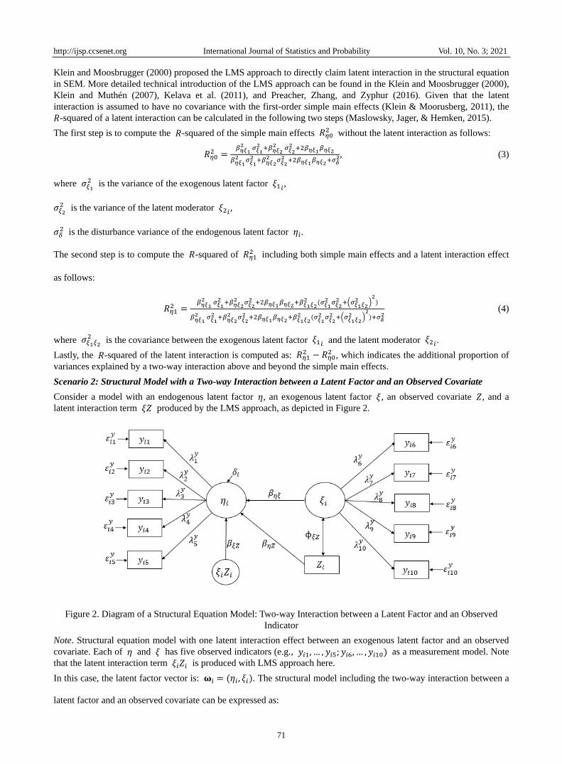
Scenario 2: Structural Model with a Two-way Interaction between a Latent Factor and an Observed Covariate
Consider a model with an endogenous latent factor 𝜂, an exogenous latent factor 𝜉, an observed covariate 𝑍, and a
latent interaction term 𝜉𝑍 produced by the LMS approach, as depicted in Figure 2.
Figure 2. Diagram of a Structural Equation Model: Two-way Interaction between a Latent Factor and an Observed
Indicator
Note. Structural equation model with one latent interaction effect between an exogenous latent factor and an observed
covariate. Each of 𝜂 and 𝜉 has five observed indicators (e.g., 𝑦𝑖1, … , 𝑦𝑖5; 𝑦𝑖6, … , 𝑦𝑖10) as a measurement model. Note
that the latent interaction term 𝜉𝑖𝑍𝑖 is produced with LMS approach here.
In this case, the latent factor vector is: 𝛚i = (𝜂𝑖 , 𝜉𝑖). The structural model including the two-way interaction between a
latent factor and an observed covariate can be expressed as:

http://ijsp.ccsenet.org International Journal of Statistics and Probability Vol. 10, No. 3; 2021
72
𝜂𝑖 = 𝛼 + 𝛽𝜂𝜉𝑍𝑖 + 𝛽𝜂𝑍𝑍𝑖 + 𝛽𝜉𝑍𝜉𝑖𝑍𝑖 + 𝛿𝑖, (5)
where 𝛽𝜂𝜉 is the regression coefficient assessing the effect of the exogenous latent factor 𝜉𝑖 on the endogenous latent
factor 𝜂𝑖,
𝛽𝜂𝑍 is the regression coefficient assessing the effect of the observed covariate 𝑍𝑖 on the endogenous latent factor 𝜂𝑖,
𝛽𝜉𝑍 is the regression coefficient measuring the latent interaction effect 𝜉𝑖𝑍𝑖 on the endogenous latent factor 𝜂𝑖.
Similar to the computation between latent factors in Equations (3) and (4), the 𝑅-squared estimation of a latent
interaction between a latent factor and a covariate is also computed as 𝑅𝜂12 − 𝑅𝜂0
2 , with 𝜉 replaced by Z when
computing 𝑅𝜂12 and 𝑅𝜂0
2 , respectively:
𝑅𝜂02 =
𝛽𝜂𝜉 2 𝜎𝜉
2+𝛽𝜂𝑍2 𝜎𝑍
2+2𝛽𝜂𝜉𝛽𝜂𝑍
𝛽𝜂𝜉2 𝜎𝜉
2+𝛽𝜂𝑍2 𝜎𝑍
2+2𝛽𝜂𝜉𝛽𝜂𝑍+𝜎𝛿2, (2)
𝑅𝜂12 =
𝛽𝜂𝜉 2 𝜎𝜉
2+𝛽𝜂𝑍2 𝜎𝑍
2+2𝛽𝜂𝜉𝛽𝜂𝑍+𝛽𝜉𝑍2 (𝜎𝜉
2𝜎𝑍2+(𝜎𝜉𝑍
2 )2
)
𝛽𝜂𝜉2 𝜎𝜉
2+𝛽𝜂𝑍2 𝜎𝑍
2+2𝛽𝜂𝜉𝛽𝜂𝑍+𝛽𝜉𝑍2 (𝜎𝜉
2𝜎𝑍2+(𝜎𝜉𝑍
2 )2
)+𝜎𝛿2, (7)
where 𝜎𝑍2 is the variance of the observed covariate 𝑍𝑖,
𝜎𝜉𝑍2 is the covariance between the exogenous latent factor 𝜉𝑖 and the observed indicator 𝑍𝑖.
The IRmplus Package
Two-way latent interactions are common in social science research and the modeling of latent interactions has brought
increasing attention. The LIR and LOIR functions in the IRmplus package were developed to compute the 𝑅-squared of a
single two-way latent interaction in the SEM given the Mplus output, following Equations (1) through (7). The LMS
approach, implemented using the XWITH command in Mplus, is one popular method to estimate the two-way
interactions, whereas the Mplus output lacks the effect size estimates unless fitting to a dataset with all variables
standardized. To employ IRmplus, Two Mplus outputs are necessary: one for the model without the latent interaction,
and one for the model including the latent interaction. IRmplus reads needed parameter estimates from the Mplus
outputs and uses them as the input to compute latent interaction effects. Table 1 presents two functions, LIR and LOIR,
included in the IRmplus package, that compute the 𝑅-squared of a latent interaction for the two scenarios discussed
above.
Table 1. Functions included in the IRmplus package
Function Approach Details
LIR LMS Compute 𝑅2of an interaction effect between two
latent factors in SEM model in Mplus
LOIR LMS Compute 𝑅2of an interaction effect between a
latent factor and an observed variable in SEM
model in Mplus
The LIR and LOIR functions were developed to compute the 𝑅-squared of a latent interaction one at a time. If multiple
two-way interactions exist in the structural model, the LIR and/or LOIR functions can be executed multiple times to
obtain the unique proportion of variances explained by the individual latent interaction.
The LIR and LOIR functions include six main arguments. The “M0” reads the Mplus output containing only simple main
effects. The “M1” reads the Mplus output containing both simple main effects and latent interaction effects. The
“endogenous” is the endogenous latent factor shown on the Mplus output. The “exogenous” is the exogenous latent
factor shown on the Mplus output. The “moderator” is the moderator variable shown on the Mplus output, which can be
a latent factor or an observed covariate in the structural model. The “interaction” is the interaction term produced by the
XWITH function and shown on the Mplus output. The two examples below present the Mplus and R scripts for
computing the latent interaction 𝑅2 using the IRmplus package.
Two-way Interaction between Latent Factors
To demonstrate the utility of functions in the IRmplus package, we simulated two data sets to provide step-by-step
guide to computing the two-way interaction between latent factors in a SEM model1. The first dataset is read as
“Example1.dat”. The data generation model contains three latent factors and 15 observed indicators (𝑦1, … , 𝑦15), where
1 Examples (data and Mplus code) are available at https://github.com/luluqinqin/IRmplus/tree/master/Examples.
http://ijsp.ccsenet.org International Journal of Statistics and Probability Vol. 10, No. 3; 2021
73
𝑦1 to 𝑦5 measure the exogenous latent factor F1, 𝑦6 to 𝑦10 measure the latent moderator F2, and 𝑦11 to 𝑦15
measure the endogenous latent factor F3. In the structural model, F3 is regressed on F1, F2, and the interaction term
between F1 and F2. We use F in this section to label latent variables because this is a common label Mplus reads for the
latent variables. The F1, F2, and F3 here correspond to the 𝜉1, 𝜉2, and 𝜂 in Equations (2) through (4).
Because IRmplus is published on GitHub, the devtools package is required before installing and loading the IRmplus
package from GitHub2. The IRmplus package is built upon the MplusAutomation, stringr, tidyverse, and stringi packages
and it only needs to be installed once. However, loading the packages (library()) is needed every time when the R
program starts.
install.packages("devtools")
library(devtools)
install_github("luluqinqin/IRmplus")
library(IRmplus)
Next, we need to prepare the Mplus syntax following a two-step procedure. First, a three-factor SEM model without
interactions is fitted, where the endogenous latent factor F3 is regressed on the exogenous latent factors F1 and F2. The
syntax is presented below and needs to be saved as an external Mplus input file (e.g., “SEM_NoINT.inp”).
TITLE: 3 Factor SEM-Without Interaction;
DATA: FILE = "example1.dat";
VARIABLE:
NAMES ARE ID y1-y15;
USEVARIABLES ARE y1-y15;
ANALYSIS:
TYPE = RANDOM;
ALGORITHM = INTEGRATION;
MODEL:
F1 BY y1 y2 y3 y4 y5;
F2 BY y6 y7 y8 y9 y10;
F3 BY y11 y12 y13 y14 y15;
F3 ON F1 F2;
OUTPUT: SAMPSTAT;
Second, we prepare the syntax for the three-factor SEM model with a two-way latent interaction to estimate the
interaction effect between exogenous latent factors F1 and F2. The syntax is shown below and saved as another external
Mplus input file (e.g., “SEM_INT.inp”).
TITLE: 3 Factor SEM-With Interaction;
DATA: FILE = "example1.dat";
VARIABLE:
NAMES ARE ID y1-y15;
USEVARIABLES ARE y1-y15;
ANALYSIS:
TYPE = RANDOM;
ALGORITHM = INTEGRATION;
MODEL:
F1 BY y1 y2 y3 y4 y5;
2 Please make sure the toolchain bundle “Rtools” (https://cran.r-project.org/bin/windows/Rtools/ ) is installed in the R
before installing the devtools package.

http://ijsp.ccsenet.org International Journal of Statistics and Probability Vol. 10, No. 3; 2021
74
F2 BY y6 y7 y8 y9 y10;
F3 BY y11 y12 y13 y14 y15;
Inter | F1 XWITH F2;
F3 ON F1 F2 Inter;
OUTPUT: SAMPSTAT;
After running the two Mplus input files, we obtain two Mplus output files (e.g., “sem_noint.out”, “sem_int.out”), which
will serve as the inputs for running the LIR function. Because the interaction is between two latent factors, the LIR
function from the IRmplus is used to calculate the 𝑅-squared of the latent interaction between F1 and F2 following the
command below.
LIR (M0 = “sem_noint.out”, M1 = “sem_int.out”, endogenous = “F3”, exogenous = “F1”, moderator = “F2”, interaction = “INTER”)
> 0.127
In the LIR function arguments, the exogenous latent factor is “F1”, the moderator is “F2”, the endogenous latent factor is
“F3”, and the interaction term “INTER” is produced by XWITH function in Mplus syntax. It is to note that the R script is
case-sensitive so that the IRmplus arguments (e.g., “INTER”) need to be the same as that shown on the Mplus output. In
this example, the LIR function returns the 𝑅-squared of a latent interaction as 0.127, which indicates that the two-way
latent interaction explains around 13% additional variances above and beyond the simple main effects of exogenous
latent factors.
Two-way Interaction between a Latent Variable and an Observed Covariate
To use the LOIR function in the IRmplus package for the computation of the 𝑅-squared of the latent interaction between
a latent factor and an observed covariate using the second simulated dataset “Example2.dat”. The data generation model
contains 15 observed indicators measuring three latent factors (the same measurement model as that in example 1) and
one binary covariate (Gender). In the structural model, F3 is regressed on F1, F2, Gender, and the interaction term
between F1 and Gender. The F1, F3, and Gender here correspond to the 𝜉, 𝜂, and Z in Equations (5) through (7).
We only present the MODEL command in the Mplus syntax below, as other commands are similar to those in the first
example. The same two-step procedure is followed. First, the model with only the main effects is fitted and the syntax is
saved (e.g., “SEM2_NoINT.inp).
MODEL
F1 BY y1 y2 y3 y4 y5;
F2 BY y6 y7 y8 y9 y10;
F3 BY y11 y12 y13 y14 y15;
F3 ON F1 F2 gender;
Second, the model with an interaction between the latent variable F1 and the observed variable gender is fitted and
saved (e.g., “SEM2_INT.inp”).
MODEL
F1 BY y1 y2 y3 y4 y5;
F2 BY y6 y7 y8 y9 y10;
F3 BY y11 y12 y13 y14 y15;
inter2 | F1 XWITH gender;
F3 ON F1 F2 gender inter2;
F1 WITH gender;
The WITH function in the Mplus syntax above is used to request the covariance estimate between an exogenous latent
factor and an observed covariate. Although “F1 WITH gender” and “gender WITH F1” both provide the same covariance
estimate, the LOIR function only supports the syntax starting with the exogenous latent factor, which is “F1 WITH gender”
in this example.
In the LOIR function arguments, the exogenous latent factor is “F1”, the moderator is “GENDER”, the endogenous latent
factor is “F3”, and the interaction term is “INTER2”. To match the variable names printed on the Mplus output, the
moderator and interaction term are both capitalized in the LOIR function. The 𝑅-squared estimation is computed as
http://ijsp.ccsenet.org International Journal of Statistics and Probability Vol. 10, No. 3; 2021
75
0.102, indicating 10% of the variances are attributable to the latent interaction term.
LOIR (M0 = “sem2_noint.out”, M1 = “sem2_int.out”, endogenous = “F3”, exogenous = “F1”, moderator = “GENDER”, interaction = “INTER2”)
> 0.102
Discussion
The attractive features of the LIR and LOIR functions in the IRmplus package include that it minimizes errors due to
human misjudges (e.g., output misinterpretation/hand calculation), and promotes the applications and interpretations of
latent interactions in latent variable modeling. However, the IRmplus package is limited in some ways that would serve
as our future research directions. It requires multiple executions of the LIR and/or LOIR functions when multiple two-way
interactions are presented in complex modeling. Future developments of the IRmplus package include exploring the
calculation of the effect size for the 3-way latent interaction, estimation of interaction effects using other estimation
approaches (e.g., product indicator approach), and automatic computation of multiple latent interaction terms.
Conclusions
The IRmplus package connects two popular statistical programs, Mplus and R, to provide an effective computation of
latent interactions between two latent variables, or between a latent variable and an observed indicator. The current
version of IRmplus (v1.0) supports outputs from Mplus version 8. We will continue incorporating more advanced latent
variable models and developing new functions to support newly methodological developments. We hope that the
package will be a practical tool to assist researchers to better understand the impact of latent interactions. The authors
are grateful for any feedback and suggestions.
References
Bollen, K. A. (1989). Structural equations with latent variables. New York: Wiley.
https://doi.org/10.1002/9781118619179
Cham, H., West, S. G., Ma, Y., & Aiken, L. S. (2012). Estimating latent variable interactions with nonnormal observed
data: A comparison of four approaches. Multivariate Behavioral Research, 47(6), 840-876.
https://doi.org/10.1080/00273171.2012.732901
Hallquist, M. N., & Wiley, J. F. (2018). MplusAutomation: An R package for facilitating large-scale latent variable
analyses in Mplus. Structural Equation Modeling: A Multidisciplinary Journal, 25(4), 621-638.
https://doi.org/10.1080/10705511.2017.1402334
Kelava, A., & Nagengast, B. (2012). A Bayesian model for the estimation of latent interaction and quadratic effects
when latent variables are non-normally distributed. Multivariate Behavioral Research, 47(5), 717-742.
https://doi.org/10.1080/00273171.2012.715560
Kelava, A., Werner, C. S., Schermelleh-Engel, K., Moosbrugger, H., Zapf, D., Ma, Y., Cham, H., Aiken, L. S., & West,
S. G. (2011). Advanced nonlinear latent variable modeling: Distribution analytic LMS and QML estimators of
interaction and quadratic effects. Structural Equation Modeling: A Multidisciplinary Journal, 18(3), 465-491.
https://doi.org/10.1080/10705511.2011.582408
Kenny, D. A., & Judd, C. M. (1984). Estimating the nonlinear and interactive effects of latent variables. Psychological
bulletin, 96(1), 201-210. https://doi.org/10.1037/0033-2909.96.1.201
Klein, A., & Moosbrugger, H. (2000). Maximum likelihood estimation of latent interaction effects with the LMS
method. Psychometrika, 65(4), 457-474. https://doi.org/10.1007/BF02296338
Klein, A. G., & Muthén, B. O. (2007). Quasi-maximum likelihood estimation of structural equation models with
multiple interaction and quadratic effects. Multivariate Behavioral Research, 42(4), 647-673.
https://doi.org/10.1080/00273170701710205
Maslowsky, J., Jager, J., & Hemken, D. (2015). Estimating and interpreting latent variable interactions: A tutorial for
applying the latent moderated structural equations method. International Journal of Behavioral Development,
39(1), 87-96. https://doi.org/10.1177/0165025414552301
Muthén, L. K., & Muthén, B. O. (2017). 1998–2017. Mplus user’s guide. Muthén & Muthén: Los Angeles, CA.
Neyman, J., & Pearson, E. S. (1933). On the problem of the most efficient tests of statistical hypotheses. Philosophical
Transactions of the Royal Society of London A, 231(694-706), 289-337. https://doi.org/10.1098/rsta.1933.0009
Preacher, K., Zhang, Z., & Zyphur, M. J. (2016). Multilevel structural equation models for assessing moderation within
and across levels of analysis. Psychological Methods, 21(2), 189-205. https://doi.org/10.1037/met0000052

http://ijsp.ccsenet.org International Journal of Statistics and Probability Vol. 10, No. 3; 2021
76
R Core Team. (2017). R: A language and environment for statistical computing. R Foundation for Statistical Computing.
Vienna, Austria.
Schumacker, R. E., & Lomax, R. G. (2004). A beginner’s guide to structural equation modeling. Lawrence Erlbaum
Associates, New Jersey, London. https://doi.org/10.4324/9781410610904
Ullman, J. B., & Bentler, P. M. (2003). Structural equation modeling. Handbook of psychology, 607-634.
https://doi.org/10.1002/0471264385.wei0224
Copyrights
Copyright for this article is retained by the author(s), with first publication rights granted to the journal.
This is an open-access article distributed under the terms and conditions of the Creative Commons Attribution license
(http://creativecommons.org/licenses/by/4.0/).


![Estimating Structural Equation Models within a Bayesian … · Structural equation modeling (SEM; Bollen, [1]) is a key latent-variable modeling framework in the social and behavioral](https://img.pdfslide.us/doc/110x75/5c7509d809d3f2a80a8c5564/estimating-structural-equation-models-within-a-bayesian-structural-equation.jpg)