Embed Size (px)
Citation preview
Department of Data Analysis Ghent University
Structural Equation Modeling with lavaan
Yves RosseelDepartment of Data Analysis
Ghent University
Gent 9–10 January 2020
Yves Rosseel Structural Equation Modeling with lavaan 1 / 256
Department of Data Analysis Ghent University
Contents1 Introduction to SEM 5
1.1 What is SEM? . . . . . . . . . . . . . . . . . . . . . . . . . . . . 51.2 How does SEM work? . . . . . . . . . . . . . . . . . . . . . . . 121.3 A first example: a CFA with three factors . . . . . . . . . . . . . 261.4 The matrix representation of a CFA model . . . . . . . . . . . . . 291.5 A second example: the Political Democracy dataset . . . . . . . . 361.6 Model estimation . . . . . . . . . . . . . . . . . . . . . . . . . . 461.7 Model evaluation . . . . . . . . . . . . . . . . . . . . . . . . . . 471.8 Model respecification . . . . . . . . . . . . . . . . . . . . . . . . 501.9 Reporting your results . . . . . . . . . . . . . . . . . . . . . . . . 511.10 Further reading . . . . . . . . . . . . . . . . . . . . . . . . . . . 52
2 Introduction to lavaan 542.1 Software for SEM . . . . . . . . . . . . . . . . . . . . . . . . . . 542.2 The R package ‘lavaan’ . . . . . . . . . . . . . . . . . . . . . . . 552.3 The lavaan model syntax . . . . . . . . . . . . . . . . . . . . . . 602.4 lavaan: a brief user’s guide . . . . . . . . . . . . . . . . . . . . . 80
Yves Rosseel Structural Equation Modeling with lavaan 2 / 256

Department of Data Analysis Ghent University
3 Multiple groups and measurement invariance 1063.1 Meanstructures . . . . . . . . . . . . . . . . . . . . . . . . . . . 1063.2 Multiple groups . . . . . . . . . . . . . . . . . . . . . . . . . . . 1113.3 Measurement invariance . . . . . . . . . . . . . . . . . . . . . . 1133.4 What if measurement invariance can not be established? (optional) 1263.5 Measurement invariance: recent developments and references . . . 130
4 Missing data and non-normal (continuous) data 1334.1 Missing data . . . . . . . . . . . . . . . . . . . . . . . . . . . . . 1334.2 Nonnormal data and alternative estimators . . . . . . . . . . . . . 140
5 Categorical data 1515.1 Handling categorical endogenous variables . . . . . . . . . . . . 1515.2 Two approaches for handling categorical data in a SEM framework 1525.3 A limited information approach: the WLSMV estimator . . . . . . 1555.4 Using categorical variables in lavaan . . . . . . . . . . . . . . . . 1665.5 SEM vs IRT . . . . . . . . . . . . . . . . . . . . . . . . . . . . . 184
6 Longitudinal Structural Equation Modeling 186
Yves Rosseel Structural Equation Modeling with lavaan 3 / 256

Department of Data Analysis Ghent University
6.1 Repeated measures ANOVA in SEM . . . . . . . . . . . . . . . . 1906.2 Panel models for longitudinal data . . . . . . . . . . . . . . . . . 2136.3 Growth curve models . . . . . . . . . . . . . . . . . . . . . . . . 2356.4 Alternative models . . . . . . . . . . . . . . . . . . . . . . . . . 248
Yves Rosseel Structural Equation Modeling with lavaan 4 / 256

Department of Data Analysis Ghent University
1 Introduction to SEM
1.1 What is SEM?• SEM is a multivariate statistical modeling technique
• SEM allows us to test a hypothesis/model about the data
– we postulate a data-generating model– this model may or may not fit the data
• what is so special about SEM?
1. the model may contain latent variables– latent variables can be hypothetical ‘constructs’ (eg., depression)
measured by a set of indicators– latent variables can be random effects (eg., random intercepts)– error terms, missing data, . . .
2. SEM allows for indirect effects (mediation), reciprocal effects, . . .3. the model is depicted as a diagram
Yves Rosseel Structural Equation Modeling with lavaan 5 / 256

Department of Data Analysis Ghent University
univariate linear regression
1
x1
x2
x3
x4
y
εβ0
β1
β2
β3
β4
x1
x2
x3
x4
y
yi = β0 + β1xi1 + β2xi2 + β3xi3 + β4xi4 + εi (i = 1, 2, . . . , n)
Yves Rosseel Structural Equation Modeling with lavaan 6 / 256
Department of Data Analysis Ghent University
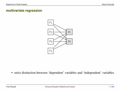
multivariate regression
x1
x2
x3
x4
y1
y2
• strict distinction between ‘dependent’ variables and ‘independent’ variables
Yves Rosseel Structural Equation Modeling with lavaan 7 / 256
Department of Data Analysis Ghent University
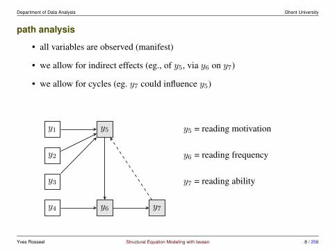
path analysis
• all variables are observed (manifest)
• we allow for indirect effects (eg., of y5, via y6 on y7)
• we allow for cycles (eg. y7 could influence y5)
y1
y2
y3
y4
y5
y6 y7
y5 = reading motivation
y6 = reading frequency
y7 = reading ability
Yves Rosseel Structural Equation Modeling with lavaan 8 / 256

Department of Data Analysis Ghent University
confirmatory factor analysis (CFA)
• measurement model: representing the relationship between one or more la-tent variables and their (observed) indicators
y1
y2
y3
y4
y5
y6
η1
η2
η1 = depression
η2 = neuroticism
Yves Rosseel Structural Equation Modeling with lavaan 9 / 256

Department of Data Analysis Ghent University
structural equation modeling (SEM)
• path analysis with latent variables
y1
y2
y3
y4
y5
y6
η1
η2
y7 y8 y9 y10 y11 y12
x1 x2 x3
η3 η4
structural part
Yves Rosseel Structural Equation Modeling with lavaan 10 / 256
Department of Data Analysis Ghent University
who is using SEM?
• it is widely used in the social sciences
• it is increasingly ‘discovered’ by other fields:
– medical sciences
– neuroimaging
– biology, ecology (climate change!)
– . . .
• SEM software is also used to perform standard analyses (eg., regression),but where there is need for:
– dealing with missing data, clustered data, categorical data
– robust standard errors, goodness-of-fit measures
– (in)equality constraints
– . . .
Yves Rosseel Structural Equation Modeling with lavaan 11 / 256

Department of Data Analysis Ghent University
1.2 How does SEM work?• we describe here the traditional SEM approach for a set of P observed (con-
tinuous) variables
• the starting point of a (traditional) SEM analysis is the observed variance-covariance matrix S of the data
– a P × P symmetric matrix– P variances are on the diagonal– P (P − 1)/2 covariances are below the diagonal (and again above the
diagonal)– a covariance represents the strength of a linear relationship between
two variables (and can be positive or negative)– if all variances would be 1, the covariances become correlations
• later, we will also include the means (y) of the observed variables
• if the data is multivariate normally distributed, then S and y contain allinformation about the data
Yves Rosseel Structural Equation Modeling with lavaan 12 / 256
Department of Data Analysis Ghent University
a dataset: the Holzinger & Swineford dataset
• this is a ‘classic’ dataset, based on data collected by Holzinger & Swineford(1939)
• scores on 26 ‘Mental Ability tests’ of seventh- and eighth-grade childrenfrom two different schools (Pasteur and Grant-White)
• the dataset was used in a seminal paper about CFA (Joreskog, 1969)
• just like Joreskog (1969), we will use a subset of 9 scores: x1 = Visualperception, x2 = Cubes, x3 = Lozenges, x4 = Paragraph comprehension, x5= Sentence completion, x6 = Word meaning, x7 = Speeded addition, x8 =Speeded counting of dots, x9 = Speeded discrimination
• these 9 scores are often regarded as indicators of 3 latent variables: ‘visualintelligence’ (x1, x2, x3), ‘textual intelligence’ (x4, x5, x6), en ‘speed’ (x7,x8, x9)
• we will investigate this later using CFA
Yves Rosseel Structural Equation Modeling with lavaan 13 / 256
Department of Data Analysis Ghent University
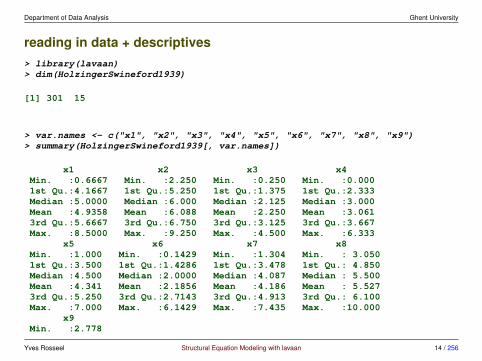
reading in data + descriptives> library(lavaan)> dim(HolzingerSwineford1939)
[1] 301 15
> var.names <- c("x1", "x2", "x3", "x4", "x5", "x6", "x7", "x8", "x9")> summary(HolzingerSwineford1939[, var.names])
x1 x2 x3 x4Min. :0.6667 Min. :2.250 Min. :0.250 Min. :0.0001st Qu.:4.1667 1st Qu.:5.250 1st Qu.:1.375 1st Qu.:2.333Median :5.0000 Median :6.000 Median :2.125 Median :3.000Mean :4.9358 Mean :6.088 Mean :2.250 Mean :3.0613rd Qu.:5.6667 3rd Qu.:6.750 3rd Qu.:3.125 3rd Qu.:3.667Max. :8.5000 Max. :9.250 Max. :4.500 Max. :6.333
x5 x6 x7 x8Min. :1.000 Min. :0.1429 Min. :1.304 Min. : 3.0501st Qu.:3.500 1st Qu.:1.4286 1st Qu.:3.478 1st Qu.: 4.850Median :4.500 Median :2.0000 Median :4.087 Median : 5.500Mean :4.341 Mean :2.1856 Mean :4.186 Mean : 5.5273rd Qu.:5.250 3rd Qu.:2.7143 3rd Qu.:4.913 3rd Qu.: 6.100Max. :7.000 Max. :6.1429 Max. :7.435 Max. :10.000
x9Min. :2.778
Yves Rosseel Structural Equation Modeling with lavaan 14 / 256

Department of Data Analysis Ghent University
1st Qu.:4.750Median :5.417Mean :5.3743rd Qu.:6.083Max. :9.250
computing the variance-covariance matrix for P = 9 variables> N <- nrow(HolzingerSwineford1939)> S <- cov( HolzingerSwineford1939[, var.names] )> S <- S * (N-1)/N # ML version> round(S, 3)
x1 x2 x3 x4 x5 x6 x7 x8 x9x1 1.358 0.407 0.580 0.505 0.441 0.455 0.085 0.264 0.458x2 0.407 1.382 0.451 0.209 0.211 0.248 -0.097 0.110 0.244x3 0.580 0.451 1.275 0.208 0.112 0.244 0.088 0.212 0.374x4 0.505 0.209 0.208 1.351 1.098 0.896 0.220 0.126 0.243x5 0.441 0.211 0.112 1.098 1.660 1.015 0.143 0.181 0.295x6 0.455 0.248 0.244 0.896 1.015 1.196 0.144 0.165 0.236x7 0.085 -0.097 0.088 0.220 0.143 0.144 1.183 0.535 0.373x8 0.264 0.110 0.212 0.126 0.181 0.165 0.535 1.022 0.457x9 0.458 0.244 0.374 0.243 0.295 0.236 0.373 0.457 1.015
Yves Rosseel Structural Equation Modeling with lavaan 15 / 256
Department of Data Analysis Ghent University
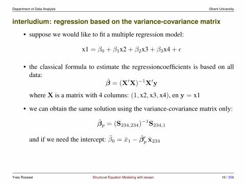
interludium: regression based on the variance-covariance matrix
• suppose we would like to fit a multiple regression model:
x1 = β0 + β1x2 + β2x3 + β3x4 + ε
• the classical formula to estimate the regressioncoefficients is based on alldata:
β = (X′X)−1X′y
where X is a matrix with 4 columns: (1, x2, x3, x4), en y = x1
• we can obtain the same solution using the variance-covariance matrix only:
βp = (S234,234)−1S234,1
and if we need the intercept: β0 = x1 − β′p x234
Yves Rosseel Structural Equation Modeling with lavaan 16 / 256
Department of Data Analysis Ghent University
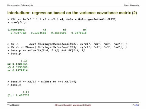
interludium: regression based on the variance-covariance matrix (2)> fit <- lm(x1 ˜ 1 + x2 + x3 + x4, data = HolzingerSwineford1939)> coef(fit)
(Intercept) x2 x3 x42.4087782 0.1324665 0.3593608 0.2978916
> SX <- cov( HolzingerSwineford1939[, c("x1", "x2", "x3", "x4")] )> MX <- colMeans( HolzingerSwineford1939[, c("x1", "x2", "x3", "x4")] )> beta.p <- solve(SX[2:4, 2:4]) %*% SX[2:4, 1]> beta.p
[,1]x2 0.1324665x3 0.3593608x4 0.2978916
> beta.0 <- MX[1] - t(beta.p) %*% MX[2:4]> beta.0
[,1][1,] 2.408778
Yves Rosseel Structural Equation Modeling with lavaan 17 / 256
Department of Data Analysis Ghent University
the model-implied variance-covariance matrix
• the goal of SEM is to test an a priori specified theory/model, based on em-pirical data; we would like to know if our model ‘fits’ the data (or not)
• each model can be depicted by a path diagram (we may have several alter-native models, each one with its own path diagram)
• each path diagram can be converted to a SEM
• SEM will tell us what the implications are for the data if (assumption!) ourmodel is correct: how ‘should’ the data look like, which patterns should weobserve?
• in practice, SEM will tell us how the variance-covariance matrix of the datashould look like; we call this the ‘model-implied’ variance-covariance ma-trix (Σ)
• different models→ different path diagrams→ different Σ matrices
• if Σ is close to S, the model fits well
Yves Rosseel Structural Equation Modeling with lavaan 18 / 256
Department of Data Analysis Ghent University
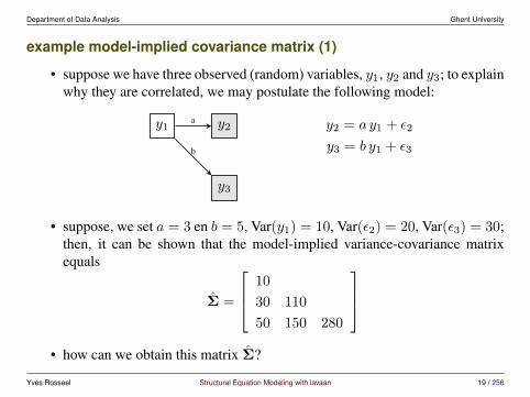
example model-implied covariance matrix (1)
• suppose we have three observed (random) variables, y1, y2 and y3; to explainwhy they are correlated, we may postulate the following model:
y1 y2
y3
a
b
y2 = a y1 + ε2
y3 = b y1 + ε3
• suppose, we set a = 3 en b = 5, Var(y1) = 10, Var(ε2) = 20, Var(ε3) = 30;then, it can be shown that the model-implied variance-covariance matrixequals
Σ =
10
30 110
50 150 280
• how can we obtain this matrix Σ?
Yves Rosseel Structural Equation Modeling with lavaan 19 / 256

Department of Data Analysis Ghent University
rules about variances and covariances
• we will apply the following rules about variances:
Var(X + Y ) = Var(X) + Var(Y ) + 2 Cov(X,Y )
Var(aX) = a2 Var(X)
• rules about covariances:
Cov(A+B,C +D) = Cov(A,C) + Cov(A,D) + Cov(B,C) + Cov(B,D)
Cov(aX, bY ) = a bCov(X,Y )
• in a regression setting, we usually assume that the predictors and the errorterms are uncorrelated: Cov(y1, ε2) = 0 and Cov(y1, ε3) = 0
• for ease of computation, we will also assume that Cov(ε2, ε3) = 0, althoughwe could easily relax this assumption
Yves Rosseel Structural Equation Modeling with lavaan 20 / 256

Department of Data Analysis Ghent University
computing the model-implied variances
• it is given that Var(y1) = 10
• the ‘model-implied’ variance of y2 is obtained as
Var(y2) = Var(a y1 + ε2)
= Var(a y1) + Var(ε2) + 2 Cov(a y1, ε2)
= Var(a y1) + Var(ε2) + 2 aCov(y1, ε2)
= Var(a y1) + Var(ε2) + 0
= a2Var(y1) + Var(ε2)
= (3)2 · 10 + 20 = 110
• similarly, the ‘model-implied’ variance of y3 is given by
Var(y3) = (5)2 · 10 + 30 = 280
Yves Rosseel Structural Equation Modeling with lavaan 21 / 256

Department of Data Analysis Ghent University
computing the model-implied covariances
• the covariance between y1 and y2:
Cov(y1, y2) = Cov(y1, a y1 + ε2)
= Cov(y1, a y1) + Cov(y1, ε2)
= aCov(y1, y1) + 0
= aVar(y1)
= 3 · 10 = 30
• similarly, Cov(y1, y3) = 5 · 10 = 50
• the covariance between y2 and y3:
Cov(y2, y3) = Cov(a y1 + ε2, b y1 + ε3)
= Cov(a y1, b y1) + Cov(a y1, ε3) + Cov(ε2, b y1) + Cov(ε2, ε3)
= a bVar(y1) + aCov(y1, ε3) + bCov(ε2, y1) + Cov(ε2, ε3)
= 3 · 5 · 10 + 3 · 0 + 5 · 0 + 0 = 150
Yves Rosseel Structural Equation Modeling with lavaan 22 / 256
Department of Data Analysis Ghent University
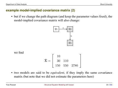
example model-implied covariance matrix (2)
• but if we change the path diagram (and keep the parameter values fixed), themodel-implied covariance matrix will also change:
y1 y2
y3
a
b
we find
Σ =
10
30 110
150 550 2780
• two models are said to be equivalent, if they imply the same covariance
matrix (but note that we did not estimate the parameters here)
Yves Rosseel Structural Equation Modeling with lavaan 23 / 256

Department of Data Analysis Ghent University
example model-implied covariance matrix (3)
• we can also postulate that the correlations among the three observed vari-ables are explained by a common ‘factor’:
y1
y2
y3
η
1
a
b
• we find using σ2(ε1) = 10, σ2(ε2) = 20, σ2(ε3) = 30, σ2(η) = 1:
Σ =
11
4 36
5 20 55
• we can compare all three Σ matrices to S to find out which model fits best
Yves Rosseel Structural Equation Modeling with lavaan 24 / 256
Department of Data Analysis Ghent University
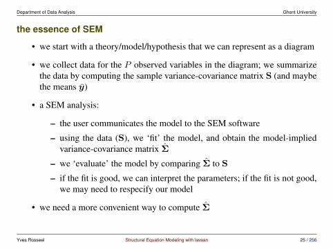
the essence of SEM
• we start with a theory/model/hypothesis that we can represent as a diagram
• we collect data for the P observed variables in the diagram; we summarizethe data by computing the sample variance-covariance matrix S (and maybethe means y)
• a SEM analysis:
– the user communicates the model to the SEM software
– using the data (S), we ‘fit’ the model, and obtain the model-impliedvariance-covariance matrix Σ
– we ‘evaluate’ the model by comparing Σ to S
– if the fit is good, we can interpret the parameters; if the fit is not good,we may need to respecify our model
• we need a more convenient way to compute Σ
Yves Rosseel Structural Equation Modeling with lavaan 25 / 256
Department of Data Analysis Ghent University
1.3 A first example: a CFA with three factors• for this example, we use the Holzinger & Swineford (1939) data
• we postulate a CFA with three latent variables (‘factors’):
– a ‘visual’ factor measured by x1, x2 and x3
– a ‘textual’ factor measured by x4, x5 and x6
– a ‘speed’ factor measured by x7, x8 and x9
• we assume the three factors are correlated
• the next slide shows a path diagram of this model
• we will discuss later how we can ‘fit’ this model using SEM software
• in the next subsection, we introduce the matrix representation of a CFAmodel, in order to have a convenient way to compute the model-impliedvariance-covariance matrix
Yves Rosseel Structural Equation Modeling with lavaan 26 / 256
Department of Data Analysis Ghent University
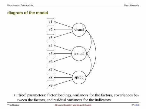
diagram of the model
x1
x2
x3
x4
x5
x6
x7
x8
x9
visual
textual
speed
• ‘free’ parameters: factor loadings, variances for the factors, covariances be-tween the factors, and residual variances for the indicators
Yves Rosseel Structural Equation Modeling with lavaan 27 / 256
Department of Data Analysis Ghent University
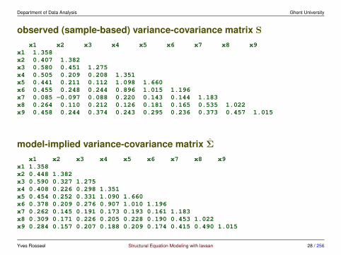
observed (sample-based) variance-covariance matrix S
x1 x2 x3 x4 x5 x6 x7 x8 x9x1 1.358x2 0.407 1.382x3 0.580 0.451 1.275x4 0.505 0.209 0.208 1.351x5 0.441 0.211 0.112 1.098 1.660x6 0.455 0.248 0.244 0.896 1.015 1.196x7 0.085 -0.097 0.088 0.220 0.143 0.144 1.183x8 0.264 0.110 0.212 0.126 0.181 0.165 0.535 1.022x9 0.458 0.244 0.374 0.243 0.295 0.236 0.373 0.457 1.015
model-implied variance-covariance matrix Σ
x1 x2 x3 x4 x5 x6 x7 x8 x9x1 1.358x2 0.448 1.382x3 0.590 0.327 1.275x4 0.408 0.226 0.298 1.351x5 0.454 0.252 0.331 1.090 1.660x6 0.378 0.209 0.276 0.907 1.010 1.196x7 0.262 0.145 0.191 0.173 0.193 0.161 1.183x8 0.309 0.171 0.226 0.205 0.228 0.190 0.453 1.022x9 0.284 0.157 0.207 0.188 0.209 0.174 0.415 0.490 1.015
Yves Rosseel Structural Equation Modeling with lavaan 28 / 256

Department of Data Analysis Ghent University
1.4 The matrix representation of a CFA model• the classic LISREL representation uses three model matrices for a CFA
• the LAMBDA matrix contains the ‘factor structure’:
Λ =
x 0 0
x 0 0
x 0 0
0 x 0
0 x 0
0 x 0
0 0 x
0 0 x
0 0 x
• the variances/covariances of the latent variables are summarized in the PSI
matrix:
Yves Rosseel Structural Equation Modeling with lavaan 29 / 256
Department of Data Analysis Ghent University
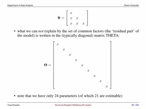
Ψ =
x
x x
x x x
• what we can not explain by the set of common factors (the ‘residual part’ of
the model) is written in the (typically diagonal) matrix THETA:
Θ =
x
x
x
x
x
x
x
x
x
• note that we have only 24 parameters (of which 21 are estimable)
Yves Rosseel Structural Equation Modeling with lavaan 30 / 256
Department of Data Analysis Ghent University
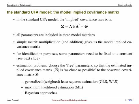
the standard CFA model: the model implied covariance matrix
• in the standard CFA model, the ‘implied’ covariance matrix is:
Σ = ΛΨΛ′ + Θ
• all parameters are included in three model matrices
• simple matrix multiplication (and addition) gives us the model implied co-variance matrix
• for identification purposes, some parameters need to be fixed to a constant(see next slide)
• estimation problem: choose the ‘free’ parameters, so that the estimated im-plied covariance matrix (Σ) is ‘as close as possible’ to the observed covari-ance matrix S
– generalized (weighted) least-squares estimation (GLS, WLS)– maximum likelihood estimation (ML)– Bayesian approaches
Yves Rosseel Structural Equation Modeling with lavaan 31 / 256
Department of Data Analysis Ghent University
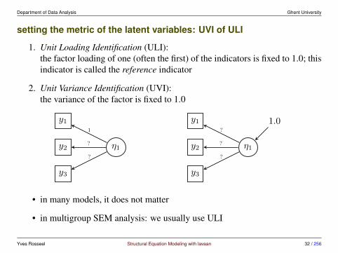
setting the metric of the latent variables: UVI of ULI
1. Unit Loading Identification (ULI):the factor loading of one (often the first) of the indicators is fixed to 1.0; thisindicator is called the reference indicator
2. Unit Variance Identification (UVI):the variance of the factor is fixed to 1.0
y1
y2
y3
η1
1
?
?
y1
y2
y3
η1
1.0?
?
?
• in many models, it does not matter
• in multigroup SEM analysis: we usually use ULI
Yves Rosseel Structural Equation Modeling with lavaan 32 / 256
Department of Data Analysis Ghent University
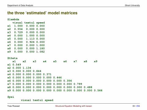
the three ‘estimated’ model matrices$lambda
visual textul speedx1 1.000 0.000 0.000x2 0.554 0.000 0.000x3 0.729 0.000 0.000x4 0.000 1.000 0.000x5 0.000 1.113 0.000x6 0.000 0.926 0.000x7 0.000 0.000 1.000x8 0.000 0.000 1.180x9 0.000 0.000 1.082
$thetax1 x2 x3 x4 x5 x6 x7 x8 x9
x1 0.549x2 0.000 1.134x3 0.000 0.000 0.844x4 0.000 0.000 0.000 0.371x5 0.000 0.000 0.000 0.000 0.446x6 0.000 0.000 0.000 0.000 0.000 0.356x7 0.000 0.000 0.000 0.000 0.000 0.000 0.799x8 0.000 0.000 0.000 0.000 0.000 0.000 0.000 0.488x9 0.000 0.000 0.000 0.000 0.000 0.000 0.000 0.000 0.566
$psivisual textul speed
Yves Rosseel Structural Equation Modeling with lavaan 33 / 256
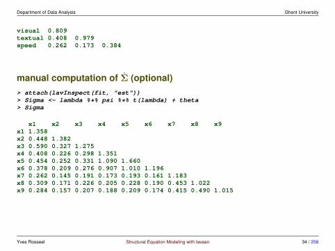
Department of Data Analysis Ghent University
visual 0.809textual 0.408 0.979speed 0.262 0.173 0.384
manual computation of Σ (optional)> attach(lavInspect(fit, "est"))> Sigma <- lambda %*% psi %*% t(lambda) + theta> Sigma
x1 x2 x3 x4 x5 x6 x7 x8 x9x1 1.358x2 0.448 1.382x3 0.590 0.327 1.275x4 0.408 0.226 0.298 1.351x5 0.454 0.252 0.331 1.090 1.660x6 0.378 0.209 0.276 0.907 1.010 1.196x7 0.262 0.145 0.191 0.173 0.193 0.161 1.183x8 0.309 0.171 0.226 0.205 0.228 0.190 0.453 1.022x9 0.284 0.157 0.207 0.188 0.209 0.174 0.415 0.490 1.015
Yves Rosseel Structural Equation Modeling with lavaan 34 / 256

Department of Data Analysis Ghent University
number of free parameters and degrees of freedom
• in our example, we have used ULI: the first factor loading (of each latentvariable) was fixed to 1.0
• therefore, we only have 21 free parameters in our model:
– 6 factor loadings– 3 variances for the factors– 3 covariances between the factors– 9 residual variances for the indicators
• our sample variance-covariance matrix (S) contains P (P +1)/2 = 45 (non-redundant) elements (‘sample statistics’)
• the difference between the number of sample statistics and the number offree parameters is called the ‘degrees of freedom’ of the model; for thismodel, we have 45− 21 = 24 degrees of freedom (df = 24)
• the number of free parameters cannot exceed the number of sample statistics;if df = 0, we say the model is ‘saturated’ because in this case Σ = S
Yves Rosseel Structural Equation Modeling with lavaan 35 / 256
Department of Data Analysis Ghent University
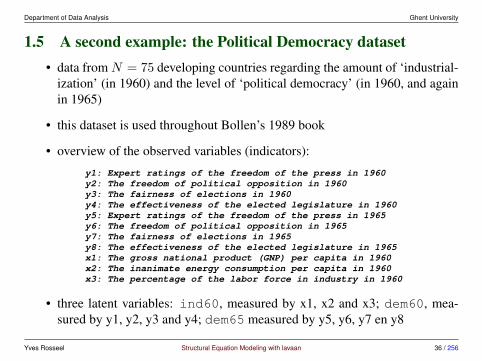
1.5 A second example: the Political Democracy dataset• data from N = 75 developing countries regarding the amount of ‘industrial-
ization’ (in 1960) and the level of ‘political democracy’ (in 1960, and againin 1965)
• this dataset is used throughout Bollen’s 1989 book
• overview of the observed variables (indicators):
y1: Expert ratings of the freedom of the press in 1960y2: The freedom of political opposition in 1960y3: The fairness of elections in 1960y4: The effectiveness of the elected legislature in 1960y5: Expert ratings of the freedom of the press in 1965y6: The freedom of political opposition in 1965y7: The fairness of elections in 1965y8: The effectiveness of the elected legislature in 1965x1: The gross national product (GNP) per capita in 1960x2: The inanimate energy consumption per capita in 1960x3: The percentage of the labor force in industry in 1960
• three latent variables: ind60, measured by x1, x2 and x3; dem60, mea-sured by y1, y2, y3 and y4; dem65 measured by y5, y6, y7 en y8
Yves Rosseel Structural Equation Modeling with lavaan 36 / 256

Department of Data Analysis Ghent University
model diagram
y1
y2
y3
y4
y5
y6
y7
y8
x1 x2 x3
dem60
dem65
ind60
Yves Rosseel Structural Equation Modeling with lavaan 37 / 256
Department of Data Analysis Ghent University
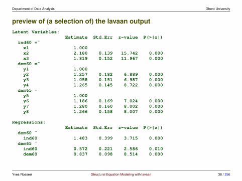
preview of (a selection of) the lavaan outputLatent Variables:
Estimate Std.Err z-value P(>|z|)ind60 =˜x1 1.000x2 2.180 0.139 15.742 0.000x3 1.819 0.152 11.967 0.000
dem60 =˜y1 1.000y2 1.257 0.182 6.889 0.000y3 1.058 0.151 6.987 0.000y4 1.265 0.145 8.722 0.000
dem65 =˜y5 1.000y6 1.186 0.169 7.024 0.000y7 1.280 0.160 8.002 0.000y8 1.266 0.158 8.007 0.000
Regressions:Estimate Std.Err z-value P(>|z|)
dem60 ˜ind60 1.483 0.399 3.715 0.000
dem65 ˜ind60 0.572 0.221 2.586 0.010dem60 0.837 0.098 8.514 0.000
Yves Rosseel Structural Equation Modeling with lavaan 38 / 256
Department of Data Analysis Ghent University
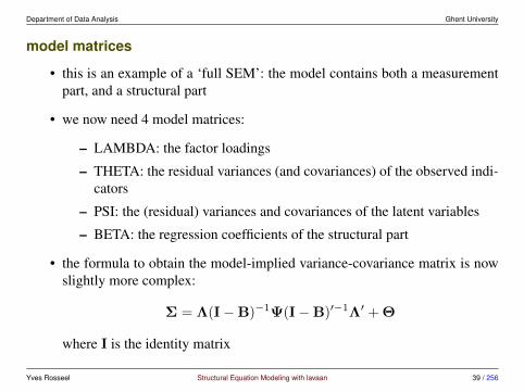
model matrices
• this is an example of a ‘full SEM’: the model contains both a measurementpart, and a structural part
• we now need 4 model matrices:
– LAMBDA: the factor loadings
– THETA: the residual variances (and covariances) of the observed indi-cators
– PSI: the (residual) variances and covariances of the latent variables
– BETA: the regression coefficients of the structural part
• the formula to obtain the model-implied variance-covariance matrix is nowslightly more complex:
Σ = Λ(I−B)−1Ψ(I−B)′−1Λ′ + Θ
where I is the identity matrix
Yves Rosseel Structural Equation Modeling with lavaan 39 / 256

Department of Data Analysis Ghent University
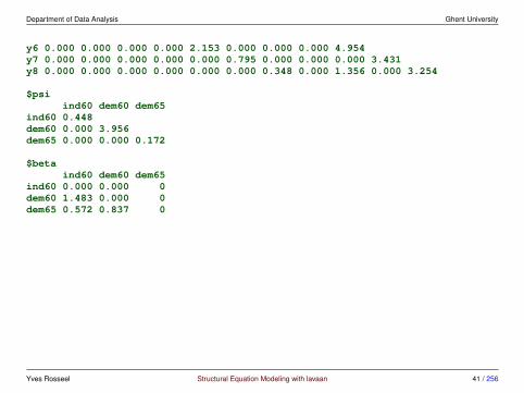
the four (already estimated) model matrices> lavInspect(fit, "est")
$lambdaind60 dem60 dem65
x1 1.000 0.000 0.000x2 2.180 0.000 0.000x3 1.819 0.000 0.000y1 0.000 1.000 0.000y2 0.000 1.257 0.000y3 0.000 1.058 0.000y4 0.000 1.265 0.000y5 0.000 0.000 1.000y6 0.000 0.000 1.186y7 0.000 0.000 1.280y8 0.000 0.000 1.266
$thetax1 x2 x3 y1 y2 y3 y4 y5 y6 y7 y8
x1 0.082x2 0.000 0.120x3 0.000 0.000 0.467y1 0.000 0.000 0.000 1.891y2 0.000 0.000 0.000 0.000 7.373y3 0.000 0.000 0.000 0.000 0.000 5.067y4 0.000 0.000 0.000 0.000 1.313 0.000 3.148y5 0.000 0.000 0.000 0.624 0.000 0.000 0.000 2.351
Yves Rosseel Structural Equation Modeling with lavaan 40 / 256
Department of Data Analysis Ghent University
y6 0.000 0.000 0.000 0.000 2.153 0.000 0.000 0.000 4.954y7 0.000 0.000 0.000 0.000 0.000 0.795 0.000 0.000 0.000 3.431y8 0.000 0.000 0.000 0.000 0.000 0.000 0.348 0.000 1.356 0.000 3.254
$psiind60 dem60 dem65
ind60 0.448dem60 0.000 3.956dem65 0.000 0.000 0.172
$betaind60 dem60 dem65
ind60 0.000 0.000 0dem60 1.483 0.000 0dem65 0.572 0.837 0
Yves Rosseel Structural Equation Modeling with lavaan 41 / 256

Department of Data Analysis Ghent University
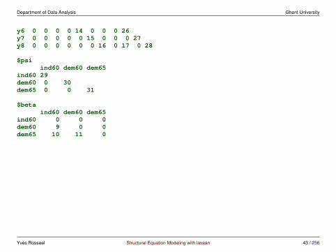
counting the 31 ‘free’ parameters in the model matrices> lavInspect(fit)
$lambdaind60 dem60 dem65
x1 0 0 0x2 1 0 0x3 2 0 0y1 0 0 0y2 0 3 0y3 0 4 0y4 0 5 0y5 0 0 0y6 0 0 6y7 0 0 7y8 0 0 8
$thetax1 x2 x3 y1 y2 y3 y4 y5 y6 y7 y8
x1 18x2 0 19x3 0 0 20y1 0 0 0 21y2 0 0 0 0 22y3 0 0 0 0 0 23y4 0 0 0 0 13 0 24y5 0 0 0 12 0 0 0 25
Yves Rosseel Structural Equation Modeling with lavaan 42 / 256
Department of Data Analysis Ghent University
y6 0 0 0 0 14 0 0 0 26y7 0 0 0 0 0 15 0 0 0 27y8 0 0 0 0 0 0 16 0 17 0 28
$psiind60 dem60 dem65
ind60 29dem60 0 30dem65 0 0 31
$betaind60 dem60 dem65
ind60 0 0 0dem60 9 0 0dem65 10 11 0
Yves Rosseel Structural Equation Modeling with lavaan 43 / 256
Department of Data Analysis Ghent University
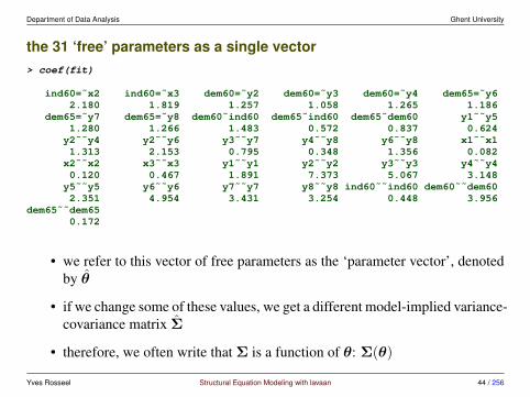
the 31 ‘free’ parameters as a single vector> coef(fit)
ind60=˜x2 ind60=˜x3 dem60=˜y2 dem60=˜y3 dem60=˜y4 dem65=˜y62.180 1.819 1.257 1.058 1.265 1.186
dem65=˜y7 dem65=˜y8 dem60˜ind60 dem65˜ind60 dem65˜dem60 y1˜˜y51.280 1.266 1.483 0.572 0.837 0.624y2˜˜y4 y2˜˜y6 y3˜˜y7 y4˜˜y8 y6˜˜y8 x1˜˜x11.313 2.153 0.795 0.348 1.356 0.082x2˜˜x2 x3˜˜x3 y1˜˜y1 y2˜˜y2 y3˜˜y3 y4˜˜y40.120 0.467 1.891 7.373 5.067 3.148y5˜˜y5 y6˜˜y6 y7˜˜y7 y8˜˜y8 ind60˜˜ind60 dem60˜˜dem602.351 4.954 3.431 3.254 0.448 3.956
dem65˜˜dem650.172
• we refer to this vector of free parameters as the ‘parameter vector’, denotedby θ
• if we change some of these values, we get a different model-implied variance-covariance matrix Σ
• therefore, we often write that Σ is a function of θ: Σ(θ)
Yves Rosseel Structural Equation Modeling with lavaan 44 / 256
Department of Data Analysis Ghent University
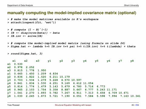
manually computing the model-implied covariance matrix (optional)> # make the model matrices available in R's workspace> attach(inspect(fit, "est"))
> # compute (I - B)ˆ(-1)> IB <- diag(nrow(beta)) - beta> IB.inv <- solve(IB)
> # compute the model-implied model matrix (using formula on slide 24)> Sigma.hat <- lambda %*% IB.inv %*% psi %*% t(IB.inv) %*% t(lambda) + theta
> round(Sigma.hat, 3)
x1 x2 x3 y1 y2 y3 y4 y5 y6 y7 y8x1 0.530x2 0.978 2.252x3 0.815 1.778 1.950y1 0.665 1.450 1.209 6.834y2 0.836 1.822 1.520 6.211 15.179y3 0.703 1.534 1.279 5.228 6.570 10.597y4 0.841 1.834 1.530 6.251 9.169 6.612 11.054y5 0.814 1.774 1.479 5.143 5.679 4.780 5.716 6.773y6 0.965 2.103 1.754 5.358 8.887 5.667 6.777 5.243 11.171y7 1.041 2.270 1.893 5.782 7.267 6.911 7.313 5.658 6.709 10.671y8 1.030 2.245 1.873 5.721 7.190 6.051 7.584 5.598 7.994 7.163 10.341
Yves Rosseel Structural Equation Modeling with lavaan 45 / 256
Department of Data Analysis Ghent University
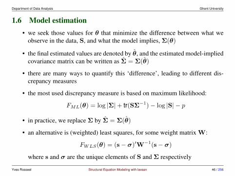
1.6 Model estimation• we seek those values for θ that minimize the difference between what we
observe in the data, S, and what the model implies, Σ(θ)
• the final estimated values are denoted by θ, and the estimated model-impliedcovariance matrix can be written as Σ = Σ(θ)
• there are many ways to quantify this ‘difference’, leading to different dis-crepancy measures
• the most used discrepancy measure is based on maximum likelihood:
FML(θ) = log |Σ|+ tr(SΣ−1)− log |S| − p
• in practice, we replace Σ by Σ = Σ(θ)
• an alternative is (weighted) least squares, for some weight matrix W:
FWLS(θ) = (s− σ)′W−1(s− σ)
where s and σ are the unique elements of S and Σ respectively
Yves Rosseel Structural Equation Modeling with lavaan 46 / 256

Department of Data Analysis Ghent University
1.7 Model evaluationevaluation of global fit – chi-square test statistic
• the chi-square test statistic is the primary test of our model
• if the chi-square test statistic is NOT significant, we have a good fit of themodel
• this becomes increasingly difficult if the sample size grows
evaluation of global fit – fit indices
• (some) rules of thumb: CFI/TLI > 0.95, RMSEA < 0.05, SRMR < 0.06
• there is a lot of controversy about the use (and misuse) of these fit indices
• a good reference is still Hu & Bentler (1999)
• current practice is to report: chi-square value + df + pvalue, RMSEA, CFIand SRMR (do not cherry pick your fit indices)
Yves Rosseel Structural Equation Modeling with lavaan 47 / 256
Department of Data Analysis Ghent University
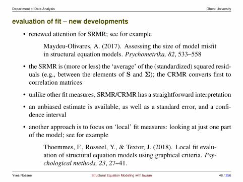
evaluation of fit – new developments
• renewed attention for SRMR; see for example
Maydeu-Olivares, A. (2017). Assessing the size of model misfitin structural equation models. Psychometrika, 82, 533–558
• the SRMR is (more or less) the ‘average’ of the (standardized) squared resid-uals (e.g., between the elements of S and Σ); the CRMR converts first tocorrelation matrices
• unlike other fit measures, SRMR/CRMR has a straightforward interpretation
• an unbiased estimate is available, as well as a standard error, and a confi-dence interval
• another approach is to focus on ‘local’ fit measures: looking at just one partof the model; see for example
Thoemmes, F., Rosseel, Y., & Textor, J. (2018). Local fit evalu-ation of structural equation models using graphical criteria. Psy-chological methods, 23, 27–41.
Yves Rosseel Structural Equation Modeling with lavaan 48 / 256

Department of Data Analysis Ghent University
admissibility of the results
• are the parameter values valid? Often a sign of a bad-fitting model
– negative (residual) variances
– correlations larger than one
• have the regression coefficients, factor loadings, covariances the proper (ex-pected) sign (positive or negative)?
• are all free parameters significant?
• are there any excessively large standard errors?
Yves Rosseel Structural Equation Modeling with lavaan 49 / 256
Department of Data Analysis Ghent University
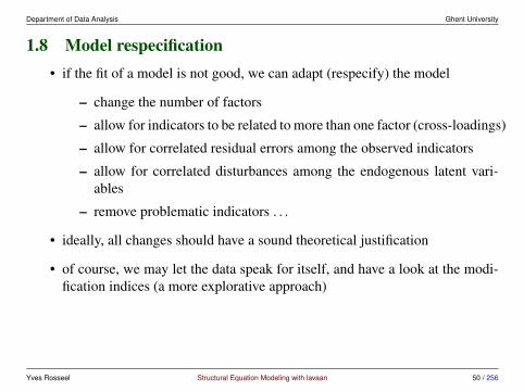
1.8 Model respecification• if the fit of a model is not good, we can adapt (respecify) the model
– change the number of factors
– allow for indicators to be related to more than one factor (cross-loadings)
– allow for correlated residual errors among the observed indicators
– allow for correlated disturbances among the endogenous latent vari-ables
– remove problematic indicators . . .
• ideally, all changes should have a sound theoretical justification
• of course, we may let the data speak for itself, and have a look at the modi-fication indices (a more explorative approach)
Yves Rosseel Structural Equation Modeling with lavaan 50 / 256

Department of Data Analysis Ghent University
1.9 Reporting your results• see Boomsma (2000)
• report enough information so that the analysis can be replicated
– always report the observed covariance matrix (or the correlation matrix+ standard deviations)
– or make sure the full dataset is available (either as an electronic ap-pendix or via a website)
Yves Rosseel Structural Equation Modeling with lavaan 51 / 256

Department of Data Analysis Ghent University
1.10 Further readingKline, R. B. (2015). Principles and practice of structural equation modeling (FourthEdition). New York: Guilford Press.
. . . The companion website supplies data, syntax, and output for the book’sexamples–now including files for Amos, EQS, LISREL, Mplus, Stata, and R(lavaan).
Brown, T. A. (2015). Confirmatory Factor Analysis for Applied Research (SecondEdition) New York: Guilford Press.
Bollen, K.A. (1989). Structural equations with latent variables. New York: Wiley.
Hancock, G. R., & Mueller, R. O. (Eds.). (2013). Structural equation modeling: Asecond course (Second Edition). Greenwich, CT: Information Age Publishing, Inc.
Boomsma, A. (2000). Reporting Analyses of Covariance Structures. StructuralEquation Modeling: A Multidisciplinary Journal, 7, 461–483.
Yves Rosseel Structural Equation Modeling with lavaan 52 / 256

Department of Data Analysis Ghent University
SEM in R, using lavaan
Gana, K., & Broc, G. (2019). Structural Equation Modeling with Lavaan. London:Wiley-ISTE.
Beaujean, A. A. (2014). Latent variable modeling using R: A step-by-step guide.New York: Routledge.
Finch, W.H., and French, B.F. (2015). Latent Variable Modeling with R. Rout-ledge.
Little, T.D. (2013). Longitudinal Structural Equation Modeling (Methodology inthe Social Sciences). The Guilford Press.
Yves Rosseel Structural Equation Modeling with lavaan 53 / 256

Department of Data Analysis Ghent University
2 Introduction to lavaan
2.1 Software for SEMsoftware for SEM: commercial – closed-source
• LISREL, EQS, AMOS, MPLUS
• SAS/Stat: proc (T)CALIS, SEPATH (Statistica), RAMONA (Systat),Stata (12 or higher)
• Mx (free, closed-source)
software for SEM: non-commercial – open-source
• outside the R ecosystem: gllamm (Stata), Onyx, . . .
• R packages: sem, OpenMx, lavaan, lava
Yves Rosseel Structural Equation Modeling with lavaan 54 / 256

Department of Data Analysis Ghent University
2.2 The R package ‘lavaan’what is lavaan?
• lavaan is an R package for latent variable analysis:
– general mean/covariance structure modeling: function lavaan()– user-friendly interface: function sem() or cfa()– support for continuous, binary and ordinal data– support for missing data, multiple groups, clustered data, . . .
• under development, future plans:
– EFA, ESEM, mixture/latent-class SEM, IRT, new engine, . . .
• the long-term goal of lavaan is
1. to implement all the state-of-the-art capabilities that are currently avail-able in commercial packages
2. to provide a modular and extensible platform that allows for easy im-plementation and testing of new statistical and modeling ideas
Yves Rosseel Structural Equation Modeling with lavaan 55 / 256

Department of Data Analysis Ghent University
installing lavaan, finding documentation
• lavaan depends on the R project for statistical computing:
http://www.r-project.org
• to install lavaan, simply start up an R session and type:
> install.packages("lavaan")
• more information about lavaan:
http://lavaan.org
• the lavaan paper:
Rosseel (2012). lavaan: an R package for structural equationmodeling. Journal of Statistical Software, 48(2), 1–36.
• lavaan discussion group (mailing list)
https://groups.google.com/d/forum/lavaan
Yves Rosseel Structural Equation Modeling with lavaan 56 / 256

Department of Data Analysis Ghent University
installing a development version of lavaan
• first install the CRAN version, to make sure you have all the dependenciesinstalled
• first method: type in R:
> install.packages("lavaan", repos = "http://www.da.ugent.be",type = "source")
• second method, using the devtools package:
> library(devtools)> install_github("yrosseel/lavaan")
• third method: if no internet, but you have a lavaan *.tar.gz file
> install.packages("c:/temp/lavaan_0.6-1.tar.gz", NULL, type = "source")
where you need to adapt the first string to point to the directory where thelavaan *.tar.gz file is located
Yves Rosseel Structural Equation Modeling with lavaan 57 / 256
Department of Data Analysis Ghent University
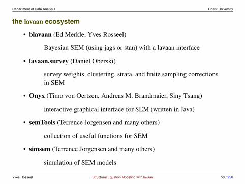
the lavaan ecosystem
• blavaan (Ed Merkle, Yves Rosseel)
Bayesian SEM (using jags or stan) with a lavaan interface
• lavaan.survey (Daniel Oberski)
survey weights, clustering, strata, and finite sampling correctionsin SEM
• Onyx (Timo von Oertzen, Andreas M. Brandmaier, Siny Tsang)
interactive graphical interface for SEM (written in Java)
• semTools (Terrence Jorgensen and many others)
collection of useful functions for SEM
• simsem (Terrence Jorgensen and many others)
simulation of SEM models
Yves Rosseel Structural Equation Modeling with lavaan 58 / 256

Department of Data Analysis Ghent University
the lavaan ecosystem (2)
• semPlot (Sacha Epskamp)
visualizations of SEM models
• EffectLiteR (Axel Mayer, Lisa Dietzfelbinger)
using SEM to estimate average and conditional effects
• MIIVsem (Zachary Fisher, Kenneth Bollen, and others)
Functions for estimating structural equation models using instru-mental variables.
• many others
bmem, coefficientalpha, eqs2lavaan, fSRM, influence.SEM, nlsem,profileR, RAMpath, regsem, RMediation, RSA, rsem, stremo,faoutlier, gimme, lavaan.shiny, matrixpls, MBESS, NlsyLinks,nonnest2, piecewiseSEM, pscore, psytabs, qgraph, sesem, sirt,TAM, userfriendlyscience, . . .
Yves Rosseel Structural Equation Modeling with lavaan 59 / 256
Department of Data Analysis Ghent University
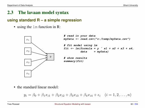
2.3 The lavaan model syntaxusing standard R – a simple regression
• using the lm function in R:
x1
x2
x3
x4
y
# read in your datamyData <- read.csv("c:/temp/myData.csv")
# fit model using lmfit <- lm(formula = y ˜ x1 + x2 + x3 + x4,
data = myData)
# show resultssummary(fit)
• the standard linear model:
yi = β0 + β1xi1 + β2xi2 + β3xi3 + β4xi4 + εi (i = 1, 2, . . . , n)
Yves Rosseel Structural Equation Modeling with lavaan 60 / 256

Department of Data Analysis Ghent University
lm() output artificial data (N=100)> summary(fit)
Call:lm(formula = y ˜ x1 + x2 + x3 + x4, data = myData)
Residuals:Min 1Q Median 3Q Max
-102.372 -29.458 -3.658 27.275 148.404
Coefficients:Estimate Std. Error t value Pr(>|t|)
(Intercept) 97.7210 4.7200 20.704 <2e-16 ***x1 5.7733 0.5238 11.022 <2e-16 ***x2 -1.3214 0.4917 -2.688 0.0085 **x3 1.1350 0.4575 2.481 0.0149 *x4 0.2707 0.4779 0.566 0.5724---Signif. codes: 0 '***' 0.001 '**' 0.01 '*' 0.05 '.' 0.1 ' ' 1
Residual standard error: 46.74 on 95 degrees of freedomMultiple R-squared: 0.5911, Adjusted R-squared: 0.5738F-statistic: 34.33 on 4 and 95 DF, p-value: < 2.2e-16
Yves Rosseel Structural Equation Modeling with lavaan 61 / 256
Department of Data Analysis Ghent University
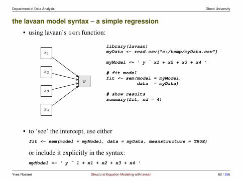
the lavaan model syntax – a simple regression
• using lavaan’s sem function:
x1
x2
x3
x4
y
library(lavaan)myData <- read.csv("c:/temp/myData.csv")
myModel <- ' y ˜ x1 + x2 + x3 + x4 '
# fit modelfit <- sem(model = myModel,
data = myData)
# show resultssummary(fit, nd = 4)
• to ‘see’ the intercept, use eitherfit <- sem(model = myModel, data = myData, meanstructure = TRUE)
or include it explicitly in the syntax:myModel <- ' y ˜ 1 + x1 + x2 + x3 + x4 '
Yves Rosseel Structural Equation Modeling with lavaan 62 / 256

Department of Data Analysis Ghent University
lavaan 0.6-3 ended normally after 32 iterations
Optimization method NLMINBNumber of free parameters 5
Number of observations 100
Estimator MLModel Fit Test Statistic 0.000Degrees of freedom 0Minimum Function Value 0.0000000000000
Parameter Estimates:
Information ExpectedInformation saturated (h1) model StructuredStandard Errors Standard
Regressions:Estimate Std.Err z-value P(>|z|)
y ˜x1 5.7733 0.5105 11.3087 0.0000x2 -1.3214 0.4792 -2.7574 0.0058x3 1.1350 0.4459 2.5451 0.0109x4 0.2707 0.4658 0.5812 0.5611
Variances:Estimate Std.Err z-value P(>|z|)
.y 2075.0999 293.4634 7.0711 0.0000
Yves Rosseel Structural Equation Modeling with lavaan 63 / 256
Department of Data Analysis Ghent University
small note: why are the standard errors (slightly) different?
• recall that in a linear model, the standard error for bj is computed by
SE(bj) =√σ2y
[(X′X)−1
]jj
• in the least-squares approach, σ2y (the residual variance of Y ) is computed
by:
σ2y =
∑ni=1(yi − yi)2
n− (p+ 1)
• if maximum likelihood is used, σ2y is computed by:
σ2y =
∑ni=1(yi − yi)2
n
and this affects the standard errors.
Yves Rosseel Structural Equation Modeling with lavaan 64 / 256
Department of Data Analysis Ghent University
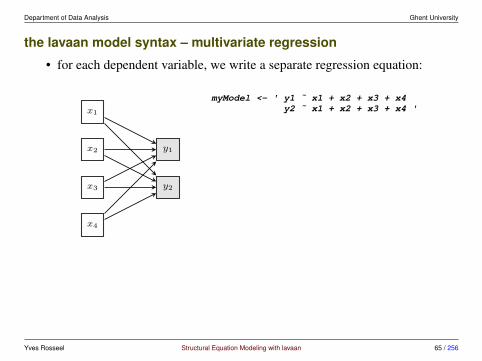
the lavaan model syntax – multivariate regression
• for each dependent variable, we write a separate regression equation:
x1
x2
x3
x4
y1
y2
myModel <- ' y1 ˜ x1 + x2 + x3 + x4y2 ˜ x1 + x2 + x3 + x4 '
Yves Rosseel Structural Equation Modeling with lavaan 65 / 256

Department of Data Analysis Ghent University
the lavaan model syntax – path analysis
• for each dependent variable, we write a separate regression equation:
x1
x2
x3
x4
x5
x6
x7
myModel <- ' x5 ˜ x1 + x2 + x3x6 ˜ x4 + x5x7 ˜ x6 '
Yves Rosseel Structural Equation Modeling with lavaan 66 / 256
Department of Data Analysis Ghent University
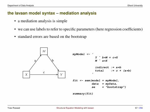
the lavaan model syntax – mediation analysis
• a mediation analysis is simple
• we can use labels to refer to specific parameters (here regression coefficients)
• standard errors are based on the bootstrap
X
M
Y
a
c
b
myModel <- 'Y ˜ b*M + c*XM ˜ a*X
indirect := a*btotal := c + (a*b)
'
fit <- sem(model = myModel,data = myData,se = "bootstrap")
summary(fit)
Yves Rosseel Structural Equation Modeling with lavaan 67 / 256

Department of Data Analysis Ghent University
partial outputParameter estimates:
Information ObservedStandard Errors BootstrapNumber of requested bootstrap draws 1000Number of successful bootstrap draws 1000
Regressions:Estimate Std.err z-value P(>|z|)
Y ˜M (b) 0.597 0.098 6.068 0.000X (c) 2.594 1.210 2.145 0.032
M ˜X (a) 2.739 0.999 2.741 0.006
Variances:Estimate Std.err z-value P(>|z|)
.Y 108.700 17.747 6.125 0.000
.M 105.408 16.556 6.367 0.000
Defined parameters:Estimate Std.err z-value P(>|z|)
indirect 1.636 0.645 2.535 0.011total 4.230 1.383 3.059 0.002
Yves Rosseel Structural Equation Modeling with lavaan 68 / 256

Department of Data Analysis Ghent University
the lavaan model syntax – using cfa() or sem()
x1
x2
x3
x4
x5
x6
x7
x8
x9
visual
textual
speed
HS.model <- ' visual =˜ x1 + x2 + x3textual =˜ x4 + x5 + x6speed =˜ x7 + x8 + x9
'
fit <- cfa(model = HS.model,data = HolzingerSwineford1939)
summary(fit, fit.measures = TRUE,standardized = TRUE)
Yves Rosseel Structural Equation Modeling with lavaan 69 / 256
Department of Data Analysis Ghent University
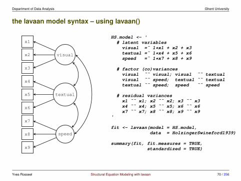
the lavaan model syntax – using lavaan()
x1
x2
x3
x4
x5
x6
x7
x8
x9
visual
textual
speed
HS.model <- '# latent variablesvisual =˜ 1*x1 + x2 + x3textual =˜ 1*x4 + x5 + x6speed =˜ 1*x7 + x8 + x9
# factor (co)variancesvisual ˜˜ visual; visual ˜˜ textualvisual ˜˜ speed; textual ˜˜ textualtextual ˜˜ speed; speed ˜˜ speed
# residual variancesx1 ˜˜ x1; x2 ˜˜ x2; x3 ˜˜ x3x4 ˜˜ x4; x5 ˜˜ x5; x6 ˜˜ x6x7 ˜˜ x7; x8 ˜˜ x8; x9 ˜˜ x9
'
fit <- lavaan(model = HS.model,data = HolzingerSwineford1939)
summary(fit, fit.measures = TRUE,standardized = TRUE)
Yves Rosseel Structural Equation Modeling with lavaan 70 / 256

Department of Data Analysis Ghent University
full outputlavaan 0.6-3 ended normally after 35 iterations
Optimization method NLMINBNumber of free parameters 21
Number of observations 301
Estimator MLModel Fit Test Statistic 85.306Degrees of freedom 24P-value (Chi-square) 0.000
Model test baseline model:
Minimum Function Test Statistic 918.852Degrees of freedom 36P-value 0.000
User model versus baseline model:
Comparative Fit Index (CFI) 0.931Tucker-Lewis Index (TLI) 0.896
Loglikelihood and Information Criteria:
Loglikelihood user model (H0) -3737.745
Yves Rosseel Structural Equation Modeling with lavaan 71 / 256
Department of Data Analysis Ghent University
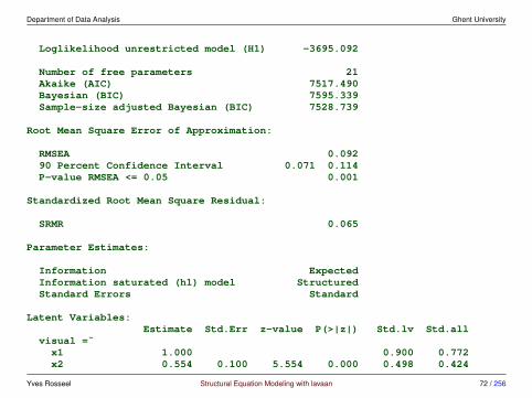
Loglikelihood unrestricted model (H1) -3695.092
Number of free parameters 21Akaike (AIC) 7517.490Bayesian (BIC) 7595.339Sample-size adjusted Bayesian (BIC) 7528.739
Root Mean Square Error of Approximation:
RMSEA 0.09290 Percent Confidence Interval 0.071 0.114P-value RMSEA <= 0.05 0.001
Standardized Root Mean Square Residual:
SRMR 0.065
Parameter Estimates:
Information ExpectedInformation saturated (h1) model StructuredStandard Errors Standard
Latent Variables:Estimate Std.Err z-value P(>|z|) Std.lv Std.all
visual =˜x1 1.000 0.900 0.772x2 0.554 0.100 5.554 0.000 0.498 0.424
Yves Rosseel Structural Equation Modeling with lavaan 72 / 256

Department of Data Analysis Ghent University
x3 0.729 0.109 6.685 0.000 0.656 0.581textual =˜x4 1.000 0.990 0.852x5 1.113 0.065 17.014 0.000 1.102 0.855x6 0.926 0.055 16.703 0.000 0.917 0.838
speed =˜x7 1.000 0.619 0.570x8 1.180 0.165 7.152 0.000 0.731 0.723x9 1.082 0.151 7.155 0.000 0.670 0.665
Covariances:Estimate Std.Err z-value P(>|z|) Std.lv Std.all
visual ˜˜textual 0.408 0.074 5.552 0.000 0.459 0.459speed 0.262 0.056 4.660 0.000 0.471 0.471
textual ˜˜speed 0.173 0.049 3.518 0.000 0.283 0.283
Variances:Estimate Std.Err z-value P(>|z|) Std.lv Std.all
.x1 0.549 0.114 4.833 0.000 0.549 0.404
.x2 1.134 0.102 11.146 0.000 1.134 0.821
.x3 0.844 0.091 9.317 0.000 0.844 0.662
.x4 0.371 0.048 7.779 0.000 0.371 0.275
.x5 0.446 0.058 7.642 0.000 0.446 0.269
.x6 0.356 0.043 8.277 0.000 0.356 0.298
.x7 0.799 0.081 9.823 0.000 0.799 0.676
.x8 0.488 0.074 6.573 0.000 0.488 0.477
Yves Rosseel Structural Equation Modeling with lavaan 73 / 256
Department of Data Analysis Ghent University
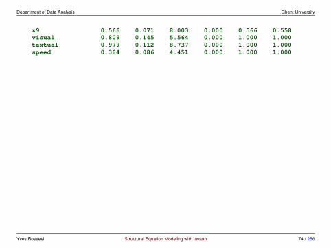
.x9 0.566 0.071 8.003 0.000 0.566 0.558visual 0.809 0.145 5.564 0.000 1.000 1.000textual 0.979 0.112 8.737 0.000 1.000 1.000speed 0.384 0.086 4.451 0.000 1.000 1.000
Yves Rosseel Structural Equation Modeling with lavaan 74 / 256
Department of Data Analysis Ghent University
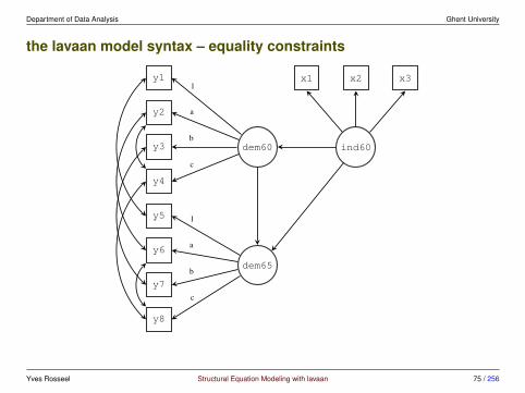
the lavaan model syntax – equality constraints
y1
y2
y3
y4
y5
y6
y7
y8
x1 x2 x3
dem60
dem65
ind60
1
a
b
c
1
a
b
c
Yves Rosseel Structural Equation Modeling with lavaan 75 / 256
Department of Data Analysis Ghent University
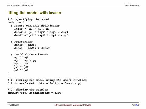
fitting the model with lavaan# 1. specifying the modelmodel <- '# latent variable definitions
ind60 =˜ x1 + x2 + x3dem60 =˜ y1 + a*y2 + b*y3 + c*y4dem65 =˜ y5 + a*y6 + b*y7 + c*y8
# regressionsdem60 ˜ ind60dem65 ˜ ind60 + dem60
# residual covariancesy1 ˜˜ y5y2 ˜˜ y4 + y6y3 ˜˜ y7y4 ˜˜ y8y6 ˜˜ y8
'
# 2. fitting the model using the sem() functionfit <- sem(model, data = PoliticalDemocracy)
# 3. display the resultssummary(fit, standardized = TRUE)
Yves Rosseel Structural Equation Modeling with lavaan 76 / 256
Department of Data Analysis Ghent University
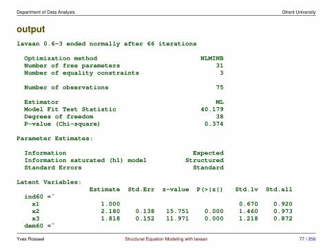
outputlavaan 0.6-3 ended normally after 66 iterations
Optimization method NLMINBNumber of free parameters 31Number of equality constraints 3
Number of observations 75
Estimator MLModel Fit Test Statistic 40.179Degrees of freedom 38P-value (Chi-square) 0.374
Parameter Estimates:
Information ExpectedInformation saturated (h1) model StructuredStandard Errors Standard
Latent Variables:Estimate Std.Err z-value P(>|z|) Std.lv Std.all
ind60 =˜x1 1.000 0.670 0.920x2 2.180 0.138 15.751 0.000 1.460 0.973x3 1.818 0.152 11.971 0.000 1.218 0.872
dem60 =˜
Yves Rosseel Structural Equation Modeling with lavaan 77 / 256

Department of Data Analysis Ghent University
y1 1.000 2.201 0.850y2 (a) 1.191 0.139 8.551 0.000 2.621 0.690y3 (b) 1.175 0.120 9.755 0.000 2.586 0.758y4 (c) 1.251 0.117 10.712 0.000 2.754 0.838
dem65 =˜y5 1.000 2.154 0.817y6 (a) 1.191 0.139 8.551 0.000 2.565 0.755y7 (b) 1.175 0.120 9.755 0.000 2.530 0.802y8 (c) 1.251 0.117 10.712 0.000 2.694 0.829
Regressions:Estimate Std.Err z-value P(>|z|) Std.lv Std.all
dem60 ˜ind60 1.471 0.392 3.750 0.000 0.448 0.448
dem65 ˜ind60 0.600 0.226 2.661 0.008 0.187 0.187dem60 0.865 0.075 11.554 0.000 0.884 0.884
Covariances:Estimate Std.Err z-value P(>|z|) Std.lv Std.all
.y1 ˜˜.y5 0.583 0.356 1.637 0.102 0.583 0.281
.y2 ˜˜.y4 1.440 0.689 2.092 0.036 1.440 0.291.y6 2.183 0.737 2.960 0.003 2.183 0.356
.y3 ˜˜.y7 0.712 0.611 1.165 0.244 0.712 0.169
.y4 ˜˜
Yves Rosseel Structural Equation Modeling with lavaan 78 / 256

Department of Data Analysis Ghent University
.y8 0.363 0.444 0.817 0.414 0.363 0.111.y6 ˜˜.y8 1.372 0.577 2.378 0.017 1.372 0.338
Variances:Estimate Std.Err z-value P(>|z|) Std.lv Std.all
.x1 0.081 0.019 4.182 0.000 0.081 0.154
.x2 0.120 0.070 1.729 0.084 0.120 0.053
.x3 0.467 0.090 5.177 0.000 0.467 0.239
.y1 1.855 0.433 4.279 0.000 1.855 0.277
.y2 7.581 1.366 5.549 0.000 7.581 0.525
.y3 4.956 0.956 5.182 0.000 4.956 0.426
.y4 3.225 0.723 4.458 0.000 3.225 0.298
.y5 2.313 0.479 4.831 0.000 2.313 0.333
.y6 4.968 0.921 5.393 0.000 4.968 0.430
.y7 3.560 0.710 5.018 0.000 3.560 0.357
.y8 3.308 0.704 4.701 0.000 3.308 0.313ind60 0.449 0.087 5.175 0.000 1.000 1.000.dem60 3.875 0.866 4.477 0.000 0.800 0.800.dem65 0.164 0.227 0.725 0.469 0.035 0.035
Yves Rosseel Structural Equation Modeling with lavaan 79 / 256

Department of Data Analysis Ghent University
2.4 lavaan: a brief user’s guidesyntax: lhs op rhs
• each line in the model syntax is a ‘formula’ and contains three parts:
– the left-hand side (‘lhs’)– the operator (‘op’)– the right-hand side (‘rhs’)
• examples:someVar ˜˜ otherVar
• the ‘+’ operator in a formula allows to collect formulas with the same lhs/rhsin a single formula; therefore
Y ˜ AY ˜ BY ˜ C
is identical toY ˜ A + B + C
Yves Rosseel Structural Equation Modeling with lavaan 80 / 256

Department of Data Analysis Ghent University
overview operators in the lavaan model syntax
formula type operator mnemonic
latent variable =˜ is manifested byregression ˜ is regressed on(residual) (co)variance ˜˜ is correlated withintercept ˜ 1 interceptthreshold | t1 first thresholdscaling factor ˜*˜ is scaled byformative latent variable <˜ is a result of
defined parameter := is defined asequality constraint == is equal toinequality constraint < is smaller thaninequality constraint > is larger than
Yves Rosseel Structural Equation Modeling with lavaan 81 / 256

Department of Data Analysis Ghent University
more syntax: modifiers
• each rhs term can be preceded by a ‘modifier’
• fixing parameters, and overriding auto-fixed parameters
HS.model.bis <- ' visual =˜ NA*x1 + x2 + x3textual =˜ NA*x4 + x5 + x6speed =˜ NA*x7 + x8 + x9visual ˜˜ 1*visualtextual ˜˜ 1*textualspeed ˜˜ 1*speed
'
• linear and nonlinear equality and inequality constraints
model.constr <- ' # model with labeled parametersy ˜ b1*x1 + b2*x2 + b3*x3
# constraintsb1 == (b2 + b3)ˆ2b1 > exp(b2 + b3) '
• several modifiers (eg. fix and label)
myModel <- ' y ˜ 0.5*x1 + x2 + x3 + b1*x1 '
Yves Rosseel Structural Equation Modeling with lavaan 82 / 256
Department of Data Analysis Ghent University
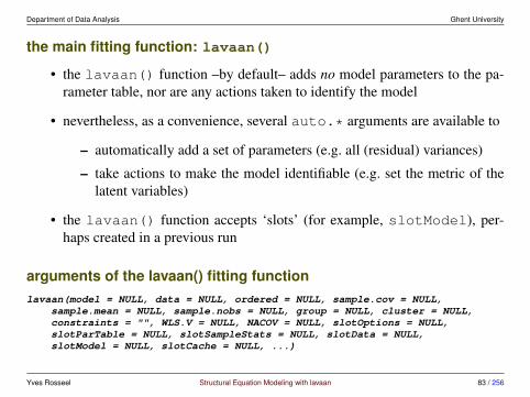
the main fitting function: lavaan()
• the lavaan() function –by default– adds no model parameters to the pa-rameter table, nor are any actions taken to identify the model
• nevertheless, as a convenience, several auto.* arguments are available to
– automatically add a set of parameters (e.g. all (residual) variances)
– take actions to make the model identifiable (e.g. set the metric of thelatent variables)
• the lavaan() function accepts ‘slots’ (for example, slotModel), per-haps created in a previous run
arguments of the lavaan() fitting functionlavaan(model = NULL, data = NULL, ordered = NULL, sample.cov = NULL,
sample.mean = NULL, sample.nobs = NULL, group = NULL, cluster = NULL,constraints = "", WLS.V = NULL, NACOV = NULL, slotOptions = NULL,slotParTable = NULL, slotSampleStats = NULL, slotData = NULL,slotModel = NULL, slotCache = NULL, ...)
Yves Rosseel Structural Equation Modeling with lavaan 83 / 256

Department of Data Analysis Ghent University
example using lavaan with an auto.* argumentHS.model.mixed <- ' # latent variables
visual =˜ 1*x1 + x2 + x3textual =˜ 1*x4 + x5 + x6speed =˜ 1*x7 + x8 + x9
# factor covariancesvisual ˜˜ textual + speedtextual ˜˜ speed
'fit <- lavaan(HS.model.mixed, data = HolzingerSwineford1939,
auto.var = TRUE)
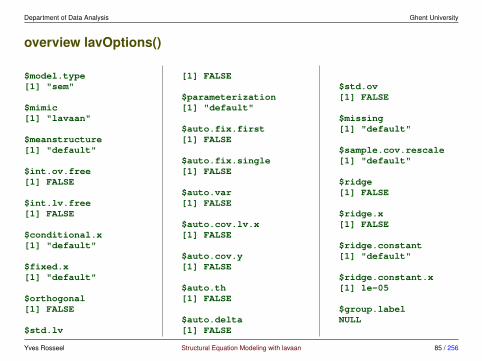
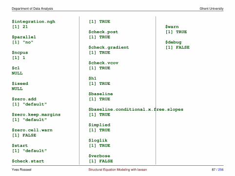
the ‘...’ argument accepts a long list of options
• see the man page of lavOptions() to get a complete overview
?lavOptions
• each of these options can be added as extra arguments to the lavaan()function
Yves Rosseel Structural Equation Modeling with lavaan 84 / 256
Department of Data Analysis Ghent University
overview lavOptions()
$model.type[1] "sem"
$mimic[1] "lavaan"
$meanstructure[1] "default"
$int.ov.free[1] FALSE
$int.lv.free[1] FALSE
$conditional.x[1] "default"
$fixed.x[1] "default"
$orthogonal[1] FALSE
$std.lv
[1] FALSE
$parameterization[1] "default"
$auto.fix.first[1] FALSE
$auto.fix.single[1] FALSE
$auto.var[1] FALSE
$auto.cov.lv.x[1] FALSE
$auto.cov.y[1] FALSE
$auto.th[1] FALSE
$auto.delta[1] FALSE
$std.ov[1] FALSE
$missing[1] "default"
$sample.cov.rescale[1] "default"
$ridge[1] FALSE
$ridge.x[1] FALSE
$ridge.constant[1] "default"
$ridge.constant.x[1] 1e-05
$group.labelNULL
Yves Rosseel Structural Equation Modeling with lavaan 85 / 256

Department of Data Analysis Ghent University
$group.equal[1] ""
$group.partial[1] ""
$group.w.free[1] FALSE
$level.labelNULL
$estimator[1] "default"
$likelihood[1] "default"
$link[1] "default"
$representation[1] "default"
$do.fit[1] TRUE
$information
[1] "default"
$h1.information[1] "structured"
$se[1] "default"
$test[1] "default"
$bootstrap[1] 1000
$observed.information[1] "hessian"
$gamma.n.minus.one[1] FALSE
$controllist()
$optim.method[1] "nlminb"
$optim.method.cor[1] "nlminb"
$optim.force.converged[1] FALSE
$optim.gradient[1] "analytic"
$optim.init_nelder_mead[1] FALSE
$optim.var.transform[1] "none"
$optim.parscale[1] "none"
$em.iter.max[1] 10000
$em.fx.tol[1] 1e-08
$em.dx.tol[1] 1e-04
$em.zerovar.offset[1] 1e-04
Yves Rosseel Structural Equation Modeling with lavaan 86 / 256
Department of Data Analysis Ghent University
$integration.ngh[1] 21
$parallel[1] "no"
$ncpus[1] 1
$clNULL
$iseedNULL
$zero.add[1] "default"
$zero.keep.margins[1] "default"
$zero.cell.warn[1] FALSE
$start[1] "default"
$check.start
[1] TRUE
$check.post[1] TRUE
$check.gradient[1] TRUE
$check.vcov[1] TRUE
$h1[1] TRUE
$baseline[1] TRUE
$baseline.conditional.x.free.slopes[1] TRUE
$implied[1] TRUE
$loglik[1] TRUE
$verbose[1] FALSE
$warn[1] TRUE
$debug[1] FALSE
Yves Rosseel Structural Equation Modeling with lavaan 87 / 256
Department of Data Analysis Ghent University
user-friendly fitting functions: sem() and cfa()
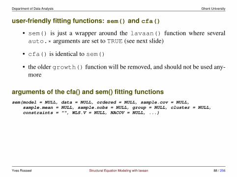
• sem() is just a wrapper around the lavaan() function where severalauto.* arguments are set to TRUE (see next slide)
• cfa() is identical to sem()
• the older growth() function will be removed, and should not be used any-more
arguments of the cfa() and sem() fitting functionssem(model = NULL, data = NULL, ordered = NULL, sample.cov = NULL,
sample.mean = NULL, sample.nobs = NULL, group = NULL, cluster = NULL,constraints = "", WLS.V = NULL, NACOV = NULL, ...)
Yves Rosseel Structural Equation Modeling with lavaan 88 / 256

Department of Data Analysis Ghent University
auto.* elements and other automatic actions
keyword operator parameter set
auto.var ˜˜ (residual) variances observed and latent variablesauto.cov.y ˜˜ (residual) covariances observed and latent endogenous vari-
ablesauto.cov.lv.x ˜˜ covariances among exogenous latent variables
keyword default action
auto.fix.first TRUE fix the factor loading of the first indicator to 1auto.fix.single TRUE fix the residual variance of a single indicator to 1int.ov.free TRUE freely estimate the intercepts of the observed variables (only
if a mean structure is included)int.lv.free FALSE freely estimate the intercepts of the latent variables (only if a
mean structure is included)
Yves Rosseel Structural Equation Modeling with lavaan 89 / 256

Department of Data Analysis Ghent University
standard R extractor functions
Method Description
summary() print a long summary of the model resultsshow() print a short summary of the model resultscoef() returns the estimates of the free parameters in the model as a named numeric vectorfitted() returns the implied moments (covariance matrix and mean vector) of the modelresid() returns the raw, normalized or standardized residuals (difference between implied
and observed moments)vcov() returns the covariance matrix of the estimated parameterspredict() compute factor scoreslogLik() returns the log-likelihood of the fitted model (if maximum likelihood estimation
was used)AIC(),BIC()
compute information criteria (if maximum likelihood estimation was used)
update() update a fitted lavaan object
Yves Rosseel Structural Equation Modeling with lavaan 90 / 256

Department of Data Analysis Ghent University
lavaan-specific extractor functions
Method Description
lavInspect() main extractor function to extract information from fitted lavaan object; by default,it returns a list of model matrices counting the free parameters in the model; canalso be used to extract starting values, sample statistics, implied statistics and muchmore
inspect() wrapper around the inspect() with some default optionslavTech() same as lavInspect() but without pretty printing; use this within scripts or
external packages
• see the man page for lavInspect() to see all the options:
?lavInspect
Yves Rosseel Structural Equation Modeling with lavaan 91 / 256
Department of Data Analysis Ghent University
other functions (1)
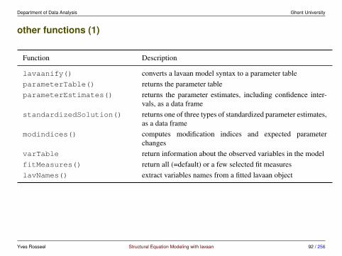
Function Description
lavaanify() converts a lavaan model syntax to a parameter tableparameterTable() returns the parameter tableparameterEstimates() returns the parameter estimates, including confidence inter-
vals, as a data framestandardizedSolution() returns one of three types of standardized parameter estimates,
as a data framemodindices() computes modification indices and expected parameter
changesvarTable return information about the observed variables in the modelfitMeasures() return all (=default) or a few selected fit measureslavNames() extract variables names from a fitted lavaan object
Yves Rosseel Structural Equation Modeling with lavaan 92 / 256

Department of Data Analysis Ghent University
other functions (2)
Function Description
lavTables() frequency tables for categorical variables and related statisticslavCor() compute polychoric, polyserial and/or Pearson correlationslavTestLRT() compare two or more (nested) models using a likelihood ratio
testlavTestWald() Wald test for testing a linear hypothesis about the parameters
of fitted lavaan objectlavTestScore() Score test (or Lagrange Multiplier test) for releasing one or
more fixed or constrained parameters in modelbootstrapLavaan() bootstrap any arbitrary statistic that can be extracted from a
fitted lavaan objectbootstrapLRT() bootstrap a chi-square difference test for comparing to alter-
native models
Yves Rosseel Structural Equation Modeling with lavaan 93 / 256
Department of Data Analysis Ghent University
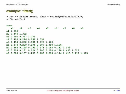
example: fitted()> fit <- cfa(HS.model, data = HolzingerSwineford1939)> fitted(fit)
$covx1 x2 x3 x4 x5 x6 x7 x8 x9
x1 1.358x2 0.448 1.382x3 0.590 0.327 1.275x4 0.408 0.226 0.298 1.351x5 0.454 0.252 0.331 1.090 1.660x6 0.378 0.209 0.276 0.907 1.010 1.196x7 0.262 0.145 0.191 0.173 0.193 0.161 1.183x8 0.309 0.171 0.226 0.205 0.228 0.190 0.453 1.022x9 0.284 0.157 0.207 0.188 0.209 0.174 0.415 0.490 1.015
Yves Rosseel Structural Equation Modeling with lavaan 94 / 256

Department of Data Analysis Ghent University
example: lavInspect()> lavInspect(fit)
$lambdavisual textul speed
x1 0 0 0x2 1 0 0x3 2 0 0x4 0 0 0x5 0 3 0x6 0 4 0x7 0 0 0x8 0 0 5x9 0 0 6
$thetax1 x2 x3 x4 x5 x6 x7 x8 x9
x1 7x2 0 8x3 0 0 9x4 0 0 0 10x5 0 0 0 0 11x6 0 0 0 0 0 12x7 0 0 0 0 0 0 13x8 0 0 0 0 0 0 0 14x9 0 0 0 0 0 0 0 0 15
Yves Rosseel Structural Equation Modeling with lavaan 95 / 256

Department of Data Analysis Ghent University
$psivisual textul speed
visual 16textual 19 17speed 20 21 18
> lavInspect(fit, "sampstat")
$covx1 x2 x3 x4 x5 x6 x7 x8 x9
x1 1.358x2 0.407 1.382x3 0.580 0.451 1.275x4 0.505 0.209 0.208 1.351x5 0.441 0.211 0.112 1.098 1.660x6 0.455 0.248 0.244 0.896 1.015 1.196x7 0.085 -0.097 0.088 0.220 0.143 0.144 1.183x8 0.264 0.110 0.212 0.126 0.181 0.165 0.535 1.022x9 0.458 0.244 0.374 0.243 0.295 0.236 0.373 0.457 1.015
> lavInspect(fit, "cov.lv")
visual textul speedvisual 0.809textual 0.408 0.979speed 0.262 0.173 0.384
Yves Rosseel Structural Equation Modeling with lavaan 96 / 256
Department of Data Analysis Ghent University
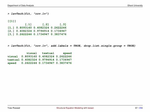
> lavTech(fit, "cov.lv")
[[1]][,1] [,2] [,3]
[1,] 0.8093160 0.4082324 0.2622246[2,] 0.4082324 0.9794914 0.1734947[3,] 0.2622246 0.1734947 0.3837476
> lavTech(fit, "cov.lv", add.labels = TRUE, drop.list.single.group = TRUE)
visual textual speedvisual 0.8093160 0.4082324 0.2622246textual 0.4082324 0.9794914 0.1734947speed 0.2622246 0.1734947 0.3837476
Yves Rosseel Structural Equation Modeling with lavaan 97 / 256

Department of Data Analysis Ghent University
example: fitMeasures()> fitMeasures(fit)
npar fmin chisq df21.000 0.142 85.306 24.000pvalue baseline.chisq baseline.df baseline.pvalue0.000 918.852 36.000 0.000
cfi tli nnfi rfi0.931 0.896 0.896 0.861
nfi pnfi ifi rni0.907 0.605 0.931 0.931logl unrestricted.logl aic bic
-3737.745 -3695.092 7517.490 7595.339ntotal bic2 rmsea rmsea.ci.lower301.000 7528.739 0.092 0.071
rmsea.ci.upper rmsea.pvalue rmr rmr_nomean0.114 0.001 0.082 0.082srmr srmr_bentler srmr_bentler_nomean crmr0.065 0.065 0.065 0.073
crmr_nomean srmr_mplus srmr_mplus_nomean cn_050.073 0.065 0.065 129.490cn_01 gfi agfi pgfi
152.654 0.943 0.894 0.503mfi ecvi
0.903 0.423
Yves Rosseel Structural Equation Modeling with lavaan 98 / 256

Department of Data Analysis Ghent University
example: parameterTable()> parameterTable(fit)[1:21,1:13]
id lhs op rhs user block group free ustart exo label plabel start1 1 visual =˜ x1 1 1 1 0 1 0 .p1. 1.0002 2 visual =˜ x2 1 1 1 1 NA 0 .p2. 0.7783 3 visual =˜ x3 1 1 1 2 NA 0 .p3. 1.1074 4 textual =˜ x4 1 1 1 0 1 0 .p4. 1.0005 5 textual =˜ x5 1 1 1 3 NA 0 .p5. 1.1336 6 textual =˜ x6 1 1 1 4 NA 0 .p6. 0.9247 7 speed =˜ x7 1 1 1 0 1 0 .p7. 1.0008 8 speed =˜ x8 1 1 1 5 NA 0 .p8. 1.2259 9 speed =˜ x9 1 1 1 6 NA 0 .p9. 0.85410 10 x1 ˜˜ x1 0 1 1 7 NA 0 .p10. 0.67911 11 x2 ˜˜ x2 0 1 1 8 NA 0 .p11. 0.69112 12 x3 ˜˜ x3 0 1 1 9 NA 0 .p12. 0.63713 13 x4 ˜˜ x4 0 1 1 10 NA 0 .p13. 0.67514 14 x5 ˜˜ x5 0 1 1 11 NA 0 .p14. 0.83015 15 x6 ˜˜ x6 0 1 1 12 NA 0 .p15. 0.59816 16 x7 ˜˜ x7 0 1 1 13 NA 0 .p16. 0.59217 17 x8 ˜˜ x8 0 1 1 14 NA 0 .p17. 0.51118 18 x9 ˜˜ x9 0 1 1 15 NA 0 .p18. 0.50819 19 visual ˜˜ visual 0 1 1 16 NA 0 .p19. 0.05020 20 textual ˜˜ textual 0 1 1 17 NA 0 .p20. 0.05021 21 speed ˜˜ speed 0 1 1 18 NA 0 .p21. 0.050
Yves Rosseel Structural Equation Modeling with lavaan 99 / 256

Department of Data Analysis Ghent University
example: parameterEstimates()> parameterEstimates(fit)[1:21,]
lhs op rhs est se z pvalue ci.lower ci.upper1 visual =˜ x1 1.000 0.000 NA NA 1.000 1.0002 visual =˜ x2 0.554 0.100 5.554 0 0.358 0.7493 visual =˜ x3 0.729 0.109 6.685 0 0.516 0.9434 textual =˜ x4 1.000 0.000 NA NA 1.000 1.0005 textual =˜ x5 1.113 0.065 17.014 0 0.985 1.2416 textual =˜ x6 0.926 0.055 16.703 0 0.817 1.0357 speed =˜ x7 1.000 0.000 NA NA 1.000 1.0008 speed =˜ x8 1.180 0.165 7.152 0 0.857 1.5039 speed =˜ x9 1.082 0.151 7.155 0 0.785 1.37810 x1 ˜˜ x1 0.549 0.114 4.833 0 0.326 0.77211 x2 ˜˜ x2 1.134 0.102 11.146 0 0.934 1.33312 x3 ˜˜ x3 0.844 0.091 9.317 0 0.667 1.02213 x4 ˜˜ x4 0.371 0.048 7.779 0 0.278 0.46514 x5 ˜˜ x5 0.446 0.058 7.642 0 0.332 0.56115 x6 ˜˜ x6 0.356 0.043 8.277 0 0.272 0.44116 x7 ˜˜ x7 0.799 0.081 9.823 0 0.640 0.95917 x8 ˜˜ x8 0.488 0.074 6.573 0 0.342 0.63318 x9 ˜˜ x9 0.566 0.071 8.003 0 0.427 0.70519 visual ˜˜ visual 0.809 0.145 5.564 0 0.524 1.09420 textual ˜˜ textual 0.979 0.112 8.737 0 0.760 1.19921 speed ˜˜ speed 0.384 0.086 4.451 0 0.215 0.553
Yves Rosseel Structural Equation Modeling with lavaan 100 / 256
Department of Data Analysis Ghent University
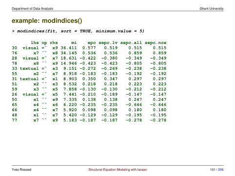
example: modindices()> modindices(fit, sort = TRUE, minimum.value = 5)
lhs op rhs mi epc sepc.lv sepc.all sepc.nox30 visual =˜ x9 36.411 0.577 0.519 0.515 0.51576 x7 ˜˜ x8 34.145 0.536 0.536 0.859 0.85928 visual =˜ x7 18.631 -0.422 -0.380 -0.349 -0.34978 x8 ˜˜ x9 14.946 -0.423 -0.423 -0.805 -0.80533 textual =˜ x3 9.151 -0.272 -0.269 -0.238 -0.23855 x2 ˜˜ x7 8.918 -0.183 -0.183 -0.192 -0.19231 textual =˜ x1 8.903 0.350 0.347 0.297 0.29751 x2 ˜˜ x3 8.532 0.218 0.218 0.223 0.22359 x3 ˜˜ x5 7.858 -0.130 -0.130 -0.212 -0.21226 visual =˜ x5 7.441 -0.210 -0.189 -0.147 -0.14750 x1 ˜˜ x9 7.335 0.138 0.138 0.247 0.24765 x4 ˜˜ x6 6.220 -0.235 -0.235 -0.646 -0.64666 x4 ˜˜ x7 5.920 0.098 0.098 0.180 0.18048 x1 ˜˜ x7 5.420 -0.129 -0.129 -0.195 -0.19577 x7 ˜˜ x9 5.183 -0.187 -0.187 -0.278 -0.278
Yves Rosseel Structural Equation Modeling with lavaan 101 / 256
Department of Data Analysis Ghent University
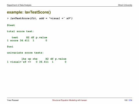
example: lavTestScore()> lavTestScore(fit, add = "visual =˜ x9")
$test
total score test:
test X2 df p.value1 score 36.411 1 0
$uni
univariate score tests:
lhs op rhs X2 df p.value1 visual=˜x9 == 0 36.411 1 0
Yves Rosseel Structural Equation Modeling with lavaan 102 / 256

Department of Data Analysis Ghent University
example: lavResiduals()> lavResiduals(fit)
$type[1] "cor.bentler"
$covx1 x2 x3 x4 x5 x6 x7 x8 x9
x1 0.000x2 -0.030 0.000x3 -0.008 0.094 0.000x4 0.071 -0.012 -0.068 0.000x5 -0.009 -0.027 -0.151 0.005 0.000x6 0.060 0.030 -0.026 -0.009 0.003 0.000x7 -0.140 -0.189 -0.084 0.037 -0.036 -0.014 0.000x8 -0.039 -0.052 -0.012 -0.067 -0.036 -0.022 0.075 0.000x9 0.149 0.073 0.147 0.048 0.067 0.056 -0.038 -0.032 0.000
$cov.zx1 x2 x3 x4 x5 x6 x7 x8 x9
x1 0.000x2 -1.996 0.000x3 -0.997 2.689 0.000x4 2.679 -0.284 -1.899 0.000x5 -0.359 -0.591 -4.157 1.545 0.000x6 2.155 0.681 -0.711 -2.588 0.942 0.000x7 -3.773 -3.654 -1.858 0.865 -0.842 -0.326 0.000
Yves Rosseel Structural Equation Modeling with lavaan 103 / 256

Department of Data Analysis Ghent University
x8 -1.380 -1.119 -0.300 -2.021 -1.099 -0.641 4.823 0.000x9 4.077 1.606 3.518 1.225 1.701 1.423 -2.325 -4.132 0.000
$summarysrmr srmr.se srmr.z srmr.pvalue usrmr usrmr.se
cov 0.065 0.006 6.063 0 0.058 0.01
Yves Rosseel Structural Equation Modeling with lavaan 104 / 256

Department of Data Analysis Ghent University
example: lavTestLRT()> fit0 <- update(fit, orthogonal = TRUE)> lavTestLRT(fit0, fit)
Chi Square Difference Test
Df AIC BIC Chisq Chisq diff Df diff Pr(>Chisq)fit 24 7517.5 7595.3 85.305fit0 27 7579.7 7646.4 153.527 68.222 3 1.026e-14 ***---Signif. codes: 0 '***' 0.001 '**' 0.01 '*' 0.05 '.' 0.1 ' ' 1
Yves Rosseel Structural Equation Modeling with lavaan 105 / 256
Department of Data Analysis Ghent University
3 Multiple groups and measurement invariance
3.1 Meanstructures• traditionally, SEM has focused on covariance structure analysis
• but we can also include the means
• typical situations where we would include the means are:
– multiple group analysis
– growth curve models
– analysis of non-normal data, and/or missing data
• we have more data: the p-dimensional mean vector
• we have more parameters:
– means/intercepts for the observed variables
– means/intercepts for the latent variables (often fixed to zero)
Yves Rosseel Structural Equation Modeling with lavaan 106 / 256
Department of Data Analysis Ghent University
adding the means in lavaan
• when the meanstructure argument is set to TRUE, a meanstructure isadded to the model
> fit <- cfa(HS.model, data = HolzingerSwineford1939,+ meanstructure = TRUE)
• if no restrictions are imposed on the means, the fit will be identical to thenon-meanstructure fit
• we add p datapoints (the mean vector)
• we add p free parameters (the intercepts of the observed variables)
• we fix the latent means to zero
• the number of degrees of freedom does not change
Yves Rosseel Structural Equation Modeling with lavaan 107 / 256
Department of Data Analysis Ghent University
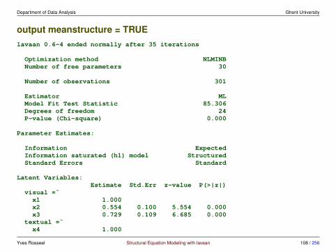
output meanstructure = TRUElavaan 0.6-4 ended normally after 35 iterations
Optimization method NLMINBNumber of free parameters 30
Number of observations 301
Estimator MLModel Fit Test Statistic 85.306Degrees of freedom 24P-value (Chi-square) 0.000
Parameter Estimates:
Information ExpectedInformation saturated (h1) model StructuredStandard Errors Standard
Latent Variables:Estimate Std.Err z-value P(>|z|)
visual =˜x1 1.000x2 0.554 0.100 5.554 0.000x3 0.729 0.109 6.685 0.000
textual =˜x4 1.000
Yves Rosseel Structural Equation Modeling with lavaan 108 / 256
Department of Data Analysis Ghent University
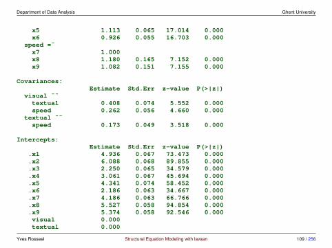
x5 1.113 0.065 17.014 0.000x6 0.926 0.055 16.703 0.000
speed =˜x7 1.000x8 1.180 0.165 7.152 0.000x9 1.082 0.151 7.155 0.000
Covariances:Estimate Std.Err z-value P(>|z|)
visual ˜˜textual 0.408 0.074 5.552 0.000speed 0.262 0.056 4.660 0.000
textual ˜˜speed 0.173 0.049 3.518 0.000
Intercepts:Estimate Std.Err z-value P(>|z|)
.x1 4.936 0.067 73.473 0.000
.x2 6.088 0.068 89.855 0.000
.x3 2.250 0.065 34.579 0.000
.x4 3.061 0.067 45.694 0.000
.x5 4.341 0.074 58.452 0.000
.x6 2.186 0.063 34.667 0.000
.x7 4.186 0.063 66.766 0.000
.x8 5.527 0.058 94.854 0.000
.x9 5.374 0.058 92.546 0.000visual 0.000textual 0.000
Yves Rosseel Structural Equation Modeling with lavaan 109 / 256
Department of Data Analysis Ghent University
speed 0.000
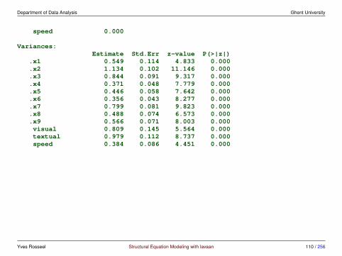
Variances:Estimate Std.Err z-value P(>|z|)
.x1 0.549 0.114 4.833 0.000
.x2 1.134 0.102 11.146 0.000
.x3 0.844 0.091 9.317 0.000
.x4 0.371 0.048 7.779 0.000
.x5 0.446 0.058 7.642 0.000
.x6 0.356 0.043 8.277 0.000
.x7 0.799 0.081 9.823 0.000
.x8 0.488 0.074 6.573 0.000
.x9 0.566 0.071 8.003 0.000visual 0.809 0.145 5.564 0.000textual 0.979 0.112 8.737 0.000speed 0.384 0.086 4.451 0.000
Yves Rosseel Structural Equation Modeling with lavaan 110 / 256
Department of Data Analysis Ghent University
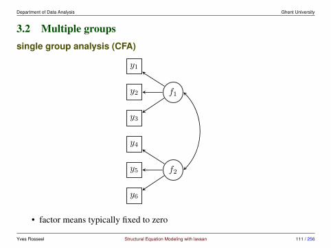
3.2 Multiple groupssingle group analysis (CFA)
y1
y2
y3
y4
y5
y6
f1
f2
• factor means typically fixed to zero
Yves Rosseel Structural Equation Modeling with lavaan 111 / 256
Department of Data Analysis Ghent University
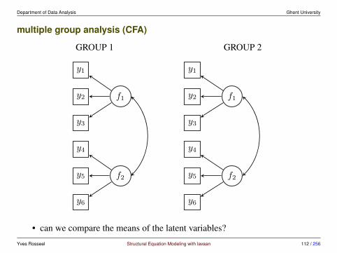
multiple group analysis (CFA)
GROUP 1 GROUP 2
y1
y2
y3
y4
y5
y6
f1
f2
y1
y2
y3
y4
y5
y6
f1
f2
• can we compare the means of the latent variables?
Yves Rosseel Structural Equation Modeling with lavaan 112 / 256
Department of Data Analysis Ghent University
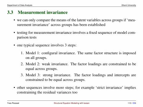
3.3 Measurement invariance• we can only compare the means of the latent variables across groups if ‘mea-
surement invariance’ across groups has been established
• testing for measurement invariance involves a fixed sequence of model com-parison tests
• one typical sequence involves 3 steps:
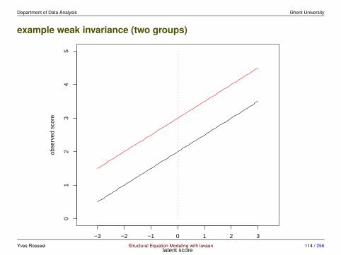
1. Model 1: configural invariance. The same factor structure is imposedon all groups.
2. Model 2: weak invariance. The factor loadings are constrained to beequal across groups.
3. Model 3: strong invariance. The factor loadings and intercepts areconstrained to be equal across groups.
• other sequences involve more steps; for example ‘strict invariance’ impliesconstraining the residual variances too
Yves Rosseel Structural Equation Modeling with lavaan 113 / 256
Department of Data Analysis Ghent University
example weak invariance (two groups)
−3 −2 −1 0 1 2 3
01
23
45
latent score
obse
rved
sco
re
Yves Rosseel Structural Equation Modeling with lavaan 114 / 256

Department of Data Analysis Ghent University
criteria to decide whether the parameter constraints are violated
• formal model comparison tests: compare the current model with the previ-ous one using a chi-square difference test (likelihood ratio test)
– may be sensitive to large sample sizes (over-powered)
• informal model comparison: compare the difference between fit measures(often CFI or RMSEA) between the current model and the previous model
– Cheung & Rensvold (2002); Chen (2007)
• look at the overall fit of the current model (either using the chi-squared test,or some fit measures)
• look at parameters of interest
– Millsap (1997), Millsap and Kwok (2004), Millsap (2007), Meuleman(2012), Oberski (2014)
Yves Rosseel Structural Equation Modeling with lavaan 115 / 256

Department of Data Analysis Ghent University
measurement invariance in lavaan - using the group.equal argument
• step 1: fit the configural invariance model (fit1)
> fit1 <- cfa(HS.model, data = HolzingerSwineford1939, group = "school")> fitMeasures(fit1, c("chisq", "df", "pvalue", "cfi", "rmsea", "srmr"))
chisq df pvalue cfi rmsea srmr115.851 48.000 0.000 0.923 0.097 0.068
• step 2: fit the weak invariance model (fit2)
> fit2 <- cfa(HS.model, data = HolzingerSwineford1939, group = "school",+ group.equal = "loadings")> fitMeasures(fit2, c("chisq", "df", "pvalue", "cfi", "rmsea", "srmr"))
chisq df pvalue cfi rmsea srmr124.044 54.000 0.000 0.921 0.093 0.072
• step 2b: compare with configural invariance model
> anova(fit1, fit2)
Yves Rosseel Structural Equation Modeling with lavaan 116 / 256
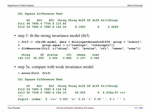
Department of Data Analysis Ghent University
Chi Square Difference Test
Df AIC BIC Chisq Chisq diff Df diff Pr(>Chisq)fit1 48 7484.4 7706.8 115.85fit2 54 7480.6 7680.8 124.04 8.1922 6 0.2244
• step 3: fit the strong invariance model (fit3)> fit3 <- cfa(HS.model, data = HolzingerSwineford1939, group = "school",+ group.equal = c("loadings", "intercepts"))> fitMeasures(fit3, c("chisq", "df", "pvalue", "cfi", "rmsea", "srmr"))
chisq df pvalue cfi rmsea srmr164.103 60.000 0.000 0.882 0.107 0.082
• step 3a: compare with weak invariance model> anova(fit2, fit3)
Chi Square Difference Test
Df AIC BIC Chisq Chisq diff Df diff Pr(>Chisq)fit2 54 7480.6 7680.8 124.04fit3 60 7508.6 7686.6 164.10 40.059 6 4.435e-07 ***---Signif. codes: 0 '***' 0.001 '**' 0.01 '*' 0.05 '.' 0.1 ' ' 1
Yves Rosseel Structural Equation Modeling with lavaan 117 / 256

Department of Data Analysis Ghent University
(optional) measurement invariance tests – manual> # configural model (manual)> HS.model.configural <- '+ visual =˜ c(1,1)*x1 + c(l2.1, l2.2)*x2 + c(l3.1, l3.2)*x3+ textual =˜ c(1,1)*x4 + c(l5.1, l5.2)*x5 + c(l6.1, l6.2)*x6+ speed =˜ c(1,1)*x7 + c(l8.1, l8.2)*x8 + c(l9.1, l9.2)*x9++ # ov intercepts+ x1 ˜ c(i1.1, i1.2)*1+ x2 ˜ c(i2.1, i2.2)*1+ x3 ˜ c(i3.1, i3.2)*1+ x4 ˜ c(i4.1, i4.2)*1+ x5 ˜ c(i5.1, i5.2)*1+ x6 ˜ c(i6.1, i6.2)*1+ x7 ˜ c(i7.1, i7.2)*1+ x8 ˜ c(i8.1, i8.2)*1+ x9 ˜ c(i9.1, i9.2)*1++ # lv means (optional, zero by default)+ visual ˜ c(0,0)*1+ textual ˜ c(0,0)*1+ speed ˜ c(0,0)*1+ '> fit1b <- cfa(HS.model.configural, data = HolzingerSwineford1939,+ group = "school")> # weak invariance model (manual)> # equal factor loadings
Yves Rosseel Structural Equation Modeling with lavaan 118 / 256
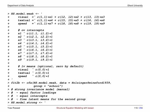
Department of Data Analysis Ghent University
> HS.model.weak <- '+ visual =˜ c(1,1)*x1 + c(l2, l2)*x2 + c(l3, l3)*x3+ textual =˜ c(1,1)*x4 + c(l5, l5)*x5 + c(l6, l6)*x6+ speed =˜ c(1,1)*x7 + c(l8, l8)*x8 + c(l9, l9)*x9++ # ov intercepts+ x1 ˜ c(i1.1, i1.2)*1+ x2 ˜ c(i2.1, i2.2)*1+ x3 ˜ c(i3.1, i3.2)*1+ x4 ˜ c(i4.1, i4.2)*1+ x5 ˜ c(i5.1, i5.2)*1+ x6 ˜ c(i6.1, i6.2)*1+ x7 ˜ c(i7.1, i7.2)*1+ x8 ˜ c(i8.1, i8.2)*1+ x9 ˜ c(i9.1, i9.2)*1++ # lv means (optional, zero by default)+ visual ˜ c(0,0)*1+ textual ˜ c(0,0)*1+ speed ˜ c(0,0)*1+ '> fit2b <- cfa(HS.model.weak, data = HolzingerSwineford1939,+ group = "school")> # strong invariance model (manual)> # - equal factor loadings> # - equal intercepts> # - free latent means for the second group> HS.model.strong <- '
Yves Rosseel Structural Equation Modeling with lavaan 119 / 256

Department of Data Analysis Ghent University
+ visual =˜ c(1,1)*x1 + c(l2, l2)*x2 + c(l3, l3)*x3+ textual =˜ c(1,1)*x4 + c(l5, l5)*x5 + c(l6, l6)*x6+ speed =˜ c(1,1)*x7 + c(l8, l8)*x8 + c(l9, l9)*x9++ # ov intercepts+ x1 ˜ c(i1, i1)*1+ x2 ˜ c(i2, i2)*1+ x3 ˜ c(i3, i3)*1+ x4 ˜ c(i4, i4)*1+ x5 ˜ c(i5, i5)*1+ x6 ˜ c(i6, i6)*1+ x7 ˜ c(i7, i7)*1+ x8 ˜ c(i8, i8)*1+ x9 ˜ c(i9, i9)*1++ # lv means+ visual ˜ c(0, NA)*1+ textual ˜ c(0, NA)*1+ speed ˜ c(0, NA)*1+ '> fit3b <- cfa(HS.model.strong, data = HolzingerSwineford1939,+ group = "school")
Yves Rosseel Structural Equation Modeling with lavaan 120 / 256
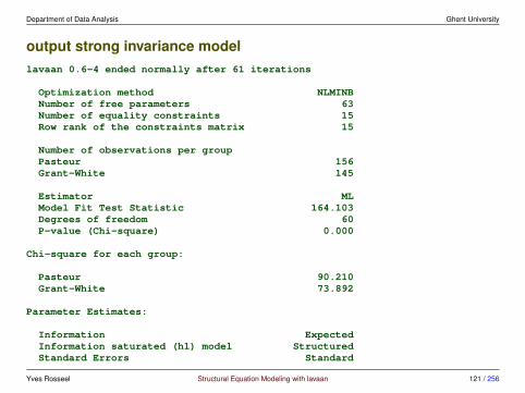
Department of Data Analysis Ghent University
output strong invariance modellavaan 0.6-4 ended normally after 61 iterations
Optimization method NLMINBNumber of free parameters 63Number of equality constraints 15Row rank of the constraints matrix 15
Number of observations per groupPasteur 156Grant-White 145
Estimator MLModel Fit Test Statistic 164.103Degrees of freedom 60P-value (Chi-square) 0.000
Chi-square for each group:
Pasteur 90.210Grant-White 73.892
Parameter Estimates:
Information ExpectedInformation saturated (h1) model StructuredStandard Errors Standard
Yves Rosseel Structural Equation Modeling with lavaan 121 / 256
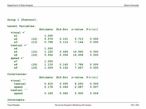
Department of Data Analysis Ghent University
Group 1 [Pasteur]:
Latent Variables:Estimate Std.Err z-value P(>|z|)
visual =˜x1 1.000x2 (l2) 0.576 0.101 5.713 0.000x3 (l3) 0.798 0.112 7.146 0.000
textual =˜x4 1.000x5 (l5) 1.120 0.066 16.965 0.000x6 (l6) 0.932 0.056 16.608 0.000
speed =˜x7 1.000x8 (l8) 1.130 0.145 7.786 0.000x9 (l9) 1.009 0.132 7.667 0.000
Covariances:Estimate Std.Err z-value P(>|z|)
visual ˜˜textual 0.410 0.095 4.293 0.000speed 0.178 0.066 2.687 0.007
textual ˜˜speed 0.180 0.062 2.900 0.004
Intercepts:
Yves Rosseel Structural Equation Modeling with lavaan 122 / 256

Department of Data Analysis Ghent University
Estimate Std.Err z-value P(>|z|).x1 (i1) 5.001 0.090 55.760 0.000.x2 (i2) 6.151 0.077 79.905 0.000.x3 (i3) 2.271 0.083 27.387 0.000.x4 (i4) 2.778 0.087 31.954 0.000.x5 (i5) 4.035 0.096 41.858 0.000.x6 (i6) 1.926 0.079 24.426 0.000.x7 (i7) 4.242 0.073 57.975 0.000.x8 (i8) 5.630 0.072 78.531 0.000.x9 (i9) 5.465 0.069 79.016 0.000visual 0.000textual 0.000speed 0.000
Variances:Estimate Std.Err z-value P(>|z|)
.x1 0.555 0.139 3.983 0.000
.x2 1.296 0.158 8.186 0.000
.x3 0.944 0.136 6.929 0.000
.x4 0.445 0.069 6.430 0.000
.x5 0.502 0.082 6.136 0.000
.x6 0.263 0.050 5.264 0.000
.x7 0.888 0.120 7.416 0.000
.x8 0.541 0.095 5.706 0.000
.x9 0.654 0.096 6.805 0.000visual 0.796 0.172 4.641 0.000textual 0.879 0.131 6.694 0.000speed 0.322 0.082 3.914 0.000
Yves Rosseel Structural Equation Modeling with lavaan 123 / 256

Department of Data Analysis Ghent University
Group 2 [Grant-White]:
Latent Variables:Estimate Std.Err z-value P(>|z|)
visual =˜x1 1.000x2 (l2) 0.576 0.101 5.713 0.000x3 (l3) 0.798 0.112 7.146 0.000
textual =˜x4 1.000x5 (l5) 1.120 0.066 16.965 0.000x6 (l6) 0.932 0.056 16.608 0.000
speed =˜x7 1.000x8 (l8) 1.130 0.145 7.786 0.000x9 (l9) 1.009 0.132 7.667 0.000
Covariances:Estimate Std.Err z-value P(>|z|)
visual ˜˜textual 0.427 0.097 4.417 0.000speed 0.329 0.082 4.006 0.000
textual ˜˜speed 0.236 0.073 3.224 0.001
Intercepts:
Yves Rosseel Structural Equation Modeling with lavaan 124 / 256

Department of Data Analysis Ghent University
Estimate Std.Err z-value P(>|z|).x1 (i1) 5.001 0.090 55.760 0.000.x2 (i2) 6.151 0.077 79.905 0.000.x3 (i3) 2.271 0.083 27.387 0.000.x4 (i4) 2.778 0.087 31.954 0.000.x5 (i5) 4.035 0.096 41.858 0.000.x6 (i6) 1.926 0.079 24.426 0.000.x7 (i7) 4.242 0.073 57.975 0.000.x8 (i8) 5.630 0.072 78.531 0.000.x9 (i9) 5.465 0.069 79.016 0.000visual -0.148 0.122 -1.211 0.226textual 0.576 0.117 4.918 0.000speed -0.177 0.090 -1.968 0.049
Variances:Estimate Std.Err z-value P(>|z|)
.x1 0.654 0.128 5.094 0.000
.x2 0.964 0.123 7.812 0.000
.x3 0.641 0.101 6.316 0.000
.x4 0.343 0.062 5.534 0.000
.x5 0.376 0.073 5.133 0.000
.x6 0.437 0.067 6.559 0.000
.x7 0.625 0.095 6.574 0.000
.x8 0.434 0.088 4.914 0.000
.x9 0.522 0.086 6.102 0.000visual 0.708 0.160 4.417 0.000textual 0.870 0.131 6.659 0.000speed 0.505 0.115 4.379 0.000
Yves Rosseel Structural Equation Modeling with lavaan 125 / 256

Department of Data Analysis Ghent University
3.4 What if measurement invariance can not be established?(optional)
1. remove some groups, and/or use subgroups instead (e.g. only a few coun-tries)
2. when is a violation of invariance large enough to warrant concern?
• sometimes, we can still retain a ranking among groups• the invariance violations may not have a substantive impact on the
comparison (see, e.g. Oberski, 2014)
3. invariance may not need to hold for all indicators/items
• partial invariance (Byrne, Shavelson & Muthen, 1989)• delete these items, or not? literature is not conclusive
4. try to explain/understand the reason why we observe non-invariance
• can we blame one or two items?• how to find these items that ‘behave’ differently
Yves Rosseel Structural Equation Modeling with lavaan 126 / 256
Department of Data Analysis Ghent University
which parameters are responsible?
• if invariance is violated, how can we accurately locate which parameters areresponsible? this turns out to be rather tricky
• one approach: use modification indices to relax equality constraints until wereach measurement invariance
– data-driven respecifications are likely to mislead, especially if manymodifications are needed (MacCallum, 1986)
– unclear how well this works in pratice
– different ways to define the metric of latent variables may have a hugeimpact
• fit a MIMIC model: a CFA model where the grouping variable (gender, age,. . . ) is included as an exogenous covariate influencing the items directly
• use person/country level predictors to ‘explain’ the differential item func-tioning (using multilevel CFA)
Yves Rosseel Structural Equation Modeling with lavaan 127 / 256
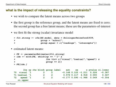
Department of Data Analysis Ghent University
what is the impact of releasing the equality constraints?
• we wish to compare the latent means across two groups
• the first group is the reference group, and the latent means are fixed to zero;the second group has a free latent means; these are the parameters-of-interest
• we first fit the strong (scalar) invariance model
> fit.strong <- cfa(HS.model, data = HolzingerSwineford1939,+ group = "school",+ group.equal = c("loadings", "intercepts"))
• estimated latent means:
> PE <- parameterEstimates(fit.strong)> idx <- with(PE, which(op == "˜1" &+ lhs %in% c("visual","textual","speed") &+ group == 2))> PE[idx,]
lhs op rhs block group label est se z pvalue ci.lower70 visual ˜1 2 2 -0.148 0.122 -1.211 0.226 -0.38771 textual ˜1 2 2 0.576 0.117 4.918 0.000 0.34772 speed ˜1 2 2 -0.177 0.090 -1.968 0.049 -0.354
ci.upper
Yves Rosseel Structural Equation Modeling with lavaan 128 / 256

Department of Data Analysis Ghent University
70 0.09171 0.80672 -0.001
• next, we ‘release’ the equality constraints, and observe by how much theparameters of interest change:
> EPC <- lavTestScore(fit.strong, epc = TRUE)$epc> idx <- with(EPC, which(op == "˜1" &+ lhs %in% c("visual","textual","speed") &+ group == 2))> EPC[idx,]
expected parameter changes (epc) and expected parameter values (epv):
lhs op rhs block group free label plabel est epc epv sepc.lv70 visual ˜1 2 2 61 .p70. -0.148 0.015 -0.133 0.01871 textual ˜1 2 2 62 .p71. 0.576 0.019 0.596 0.02172 speed ˜1 2 2 63 .p72. -0.177 0.001 -0.176 0.001
sepc.all sepc.nox70 0.018 0.01871 0.021 0.02172 0.001 0.001
Yves Rosseel Structural Equation Modeling with lavaan 129 / 256

Department of Data Analysis Ghent University
3.5 Measurement invariance: recent developments and refer-ences
• explorarory SEM (ESEM; Asparouhov & Muthen, 2009)
– cross-loadings can be non-zero
• Bayesian SEM (e.g. Muthen & Asparouhov, 2012, 2013)
– approximate (instead of strict) measurement invariance
– these methods allow for some ‘wiggle room’ across groups
• alignment (Asparouhov & Muthen, 2013)
– equality constraints are replaced by a procedure similar to rotation inEFA
Yves Rosseel Structural Equation Modeling with lavaan 130 / 256

Department of Data Analysis Ghent University
references
• technical:
– Meredith, W. (1993). Measurement invariance, factor analysis and factorialinvariance. Psychometrika, 58, 525–543.
– Millsap, R.E. (2011). Statistical approaches to measurement invariance. Rout-ledge.
• general references:
– Vandenberg, R.J. and Lance, C.E. (2000). A Review and Synthesis of the Mea-surement Invariance Literature: Suggestions, Practices, and Recommendationsfor Organizational Research. Organizational Research Methods, 3, 4–69.
– Horn, J.L., & McArdle, J.J. (1992). A practical and theoretical guide to mea-surement invariance in aging research. Experimental Aging Research, 18, 117–144.
• reviews:
– Schmitt, N., & Kuljanin, G. (2008). Measurement invariance: Review of prac-tice and implications. Human Resource Management Review, 18, 210–222.
Yves Rosseel Structural Equation Modeling with lavaan 131 / 256

Department of Data Analysis Ghent University
– Davidov, E., Meuleman, B., Cieciuch, J., Schmidt, P., & Billiet, J. (2014).Measurement equivalence in cross-national research. Annual Review of Soci-ology, 40, 55–75.
• testing strategies:
– Cheung, G.W., and Rensvold, R.B. (2000). Evaluating goodness-of-fit indicesfor testing measurement invariance. Structural Equation Modeling, 9, 233–255.
• partial invariance:
– Byrne, B.M., Shavelson, R.J and Muthen, B. (1989). Testing for the equiva-lence of factor covariance and mean structures: The issue of partial measure-ment invariance. Psychological Bulletin, 105, 456–466.
Yves Rosseel Structural Equation Modeling with lavaan 132 / 256
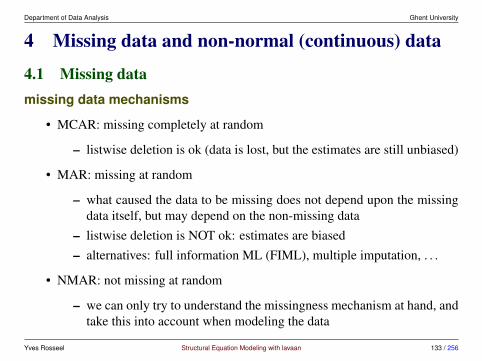
Department of Data Analysis Ghent University
4 Missing data and non-normal (continuous) data
4.1 Missing datamissing data mechanisms
• MCAR: missing completely at random
– listwise deletion is ok (data is lost, but the estimates are still unbiased)
• MAR: missing at random
– what caused the data to be missing does not depend upon the missingdata itself, but may depend on the non-missing data
– listwise deletion is NOT ok: estimates are biased– alternatives: full information ML (FIML), multiple imputation, . . .
• NMAR: not missing at random
– we can only try to understand the missingness mechanism at hand, andtake this into account when modeling the data
Yves Rosseel Structural Equation Modeling with lavaan 133 / 256
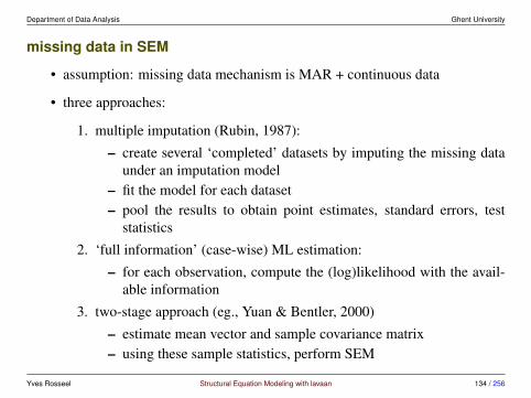
Department of Data Analysis Ghent University
missing data in SEM
• assumption: missing data mechanism is MAR + continuous data
• three approaches:
1. multiple imputation (Rubin, 1987):
– create several ‘completed’ datasets by imputing the missing dataunder an imputation model
– fit the model for each dataset– pool the results to obtain point estimates, standard errors, test
statistics
2. ‘full information’ (case-wise) ML estimation:
– for each observation, compute the (log)likelihood with the avail-able information
3. two-stage approach (eg., Yuan & Bentler, 2000)
– estimate mean vector and sample covariance matrix– using these sample statistics, perform SEM
Yves Rosseel Structural Equation Modeling with lavaan 134 / 256

Department of Data Analysis Ghent University
missing data in lavaan
• in lavaan 0.6, the default is listwise deletion (but this may change in futureversions)
lavaan 0.6-3 ended normally after 35 iterations
Used TotalNumber of observations 156 301
– the goal is to alert the user that data is missing
• available approaches in lavaan:
– ‘full information’ ML (missing = "fiml")
– two-stage approach (missing = "two.stage")
• multiple imputation in lavaan:
– create imputed datasets (eg., using the mice package) + lavaanList()
– the runMI() function in the semTools package
Yves Rosseel Structural Equation Modeling with lavaan 135 / 256

Department of Data Analysis Ghent University
example: lavaan + fiml> fit <- cfa(HS.model, data = HS.missing, missing = "fiml")> fit
lavaan 0.6-3 ended normally after 51 iterations
Optimization method NLMINBNumber of free parameters 30
Number of observations 301Number of missing patterns 13
Estimator MLModel Fit Test Statistic 85.868Degrees of freedom 24P-value (Chi-square) 0.000
> # missing patterns> lavInspect(fit, "patterns")
x1 x2 x3 x4 x5 x6 x7 x8 x9[1,] 1 1 1 1 1 1 1 1 1[2,] 1 0 1 1 1 1 1 1 1[3,] 1 1 0 1 1 1 1 1 1[4,] 0 1 1 1 1 1 1 1 1
Yves Rosseel Structural Equation Modeling with lavaan 136 / 256

Department of Data Analysis Ghent University
[5,] 1 1 1 0 1 1 1 1 1[6,] 1 1 1 1 0 1 1 1 1[7,] 1 1 1 1 1 0 1 1 1[8,] 1 1 1 1 1 1 0 1 1[9,] 1 1 1 1 1 1 1 0 1[10,] 1 1 1 1 1 1 1 1 0[11,] 0 1 1 0 1 0 1 1 1[12,] 1 1 1 1 0 1 1 0 1[13,] 1 1 1 1 1 1 0 1 0
> # percentage complete cases per pair> lavInspect(fit, "coverage")
x1 x2 x3 x4 x5 x6 x7 x8 x9x1 0.983x2 0.967 0.983x3 0.967 0.967 0.983x4 0.970 0.967 0.967 0.983x5 0.967 0.967 0.967 0.967 0.983x6 0.970 0.967 0.967 0.970 0.967 0.983x7 0.967 0.967 0.967 0.967 0.967 0.967 0.983x8 0.967 0.967 0.967 0.967 0.970 0.967 0.967 0.983x9 0.967 0.967 0.967 0.967 0.967 0.967 0.970 0.967 0.983
> # sample statistics unrestricted (h1) model> lavInspect(fit, "sampstat.h1")
Yves Rosseel Structural Equation Modeling with lavaan 137 / 256
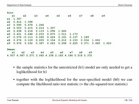
Department of Data Analysis Ghent University
$covx1 x2 x3 x4 x5 x6 x7 x8 x9
x1 1.367x2 0.412 1.398x3 0.590 0.478 1.266x4 0.503 0.215 0.214 1.357x5 0.438 0.218 0.119 1.096 1.665x6 0.431 0.248 0.233 0.875 1.011 1.173x7 0.074 -0.113 0.045 0.224 0.141 0.137 1.189x8 0.274 0.109 0.205 0.154 0.212 0.153 0.534 1.002x9 0.476 0.232 0.367 0.243 0.296 0.225 0.371 0.460 1.023
$meanx1 x2 x3 x4 x5 x6 x7 x8 x9
4.937 6.087 2.271 3.062 4.338 2.182 4.186 5.518 5.372
• the sample statistics for the unrestricted (h1) model are only needed to get aloglikelihood for h1
• together with the loglikelihood for the user-specified model (h0) we cancompute the likelihood ratio test statistic (= the chi-squared test statistic)
Yves Rosseel Structural Equation Modeling with lavaan 138 / 256

Department of Data Analysis Ghent University
example: lavaan + two.stage> fit <- cfa(HS.model, data = HS.missing, missing = "two.stage")> fit
lavaan 0.6-3 ended normally after 36 iterations
Optimization method NLMINBNumber of free parameters 30
Number of observations 301Number of missing patterns 13
Estimator ML RobustModel Fit Test Statistic 90.130 87.108Degrees of freedom 24 24P-value (Chi-square) 0.000 0.000Scaling correction factor 1.035
for the Satorra-Bentler correction
• a robust test statistic (and robust standard errors) are needed to take the two-stage estimation process into account
• outperforms ‘fiml’ in the non-normal case (see Savalei & Falk, 2014)
Yves Rosseel Structural Equation Modeling with lavaan 139 / 256
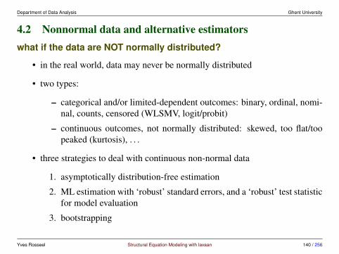
Department of Data Analysis Ghent University
4.2 Nonnormal data and alternative estimatorswhat if the data are NOT normally distributed?
• in the real world, data may never be normally distributed
• two types:
– categorical and/or limited-dependent outcomes: binary, ordinal, nomi-nal, counts, censored (WLSMV, logit/probit)
– continuous outcomes, not normally distributed: skewed, too flat/toopeaked (kurtosis), . . .
• three strategies to deal with continuous non-normal data
1. asymptotically distribution-free estimation
2. ML estimation with ‘robust’ standard errors, and a ‘robust’ test statisticfor model evaluation
3. bootstrapping
Yves Rosseel Structural Equation Modeling with lavaan 140 / 256

Department of Data Analysis Ghent University
robust method 1: asymptotically distribution-free (ADF) estimation
• the ADF estimator (Browne, 1984) makes no assumption of normality andis part of a larger family of estimators called weighted least squares (WLS)estimators:
FWLS = (s− σ)>W−1(s− σ)
where s and σ are vectors containing the non-duplicated elements in thesample (S) and model-implied (Σ) covariance matrix respectively
• the weight matrix W utilized with the ADF estimator is the asymptotic co-variance matrix: a matrix of the covariances of the observed sample vari-ances and covariances
• unfortunately, empirical research has shown that the ADF method breaksdown unless the sample size is huge (e.g., N > 5000)
• in lavaan:
fit <- cfa(HS.model, data = HolzingerSwineford1939,estimator = "WLS")
Yves Rosseel Structural Equation Modeling with lavaan 141 / 256

Department of Data Analysis Ghent University
robust method 2: robust ML
1. parameter estimates: vanilla ML
• if ML is used, the parameter estimates are still consistent (if the modelis identified and correctly specified)
2. ‘robust’ standard errors
• if data is non-normal, the standard errors tend to be too small (as muchas 25-50%)
• ‘robust’ standard errors correct for non-normality (see Appendix)
3. ‘robust’ scaled (chi-square) test statistic
• if data is non-normal, the usual model (chi-square) test statistic tendsto be too large
• the Satorra-Bentler scaled test statistic rescales the value of the ML-based chi-square test statistic by an amount that reflects the degree ofkurtosis (see Appendix)
Yves Rosseel Structural Equation Modeling with lavaan 142 / 256
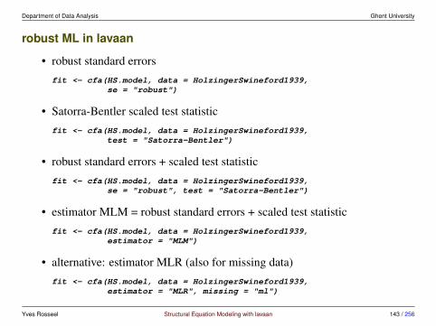
Department of Data Analysis Ghent University
robust ML in lavaan
• robust standard errorsfit <- cfa(HS.model, data = HolzingerSwineford1939,
se = "robust")
• Satorra-Bentler scaled test statisticfit <- cfa(HS.model, data = HolzingerSwineford1939,
test = "Satorra-Bentler")
• robust standard errors + scaled test statisticfit <- cfa(HS.model, data = HolzingerSwineford1939,
se = "robust", test = "Satorra-Bentler")
• estimator MLM = robust standard errors + scaled test statisticfit <- cfa(HS.model, data = HolzingerSwineford1939,
estimator = "MLM")
• alternative: estimator MLR (also for missing data)fit <- cfa(HS.model, data = HolzingerSwineford1939,
estimator = "MLR", missing = "ml")
Yves Rosseel Structural Equation Modeling with lavaan 143 / 256
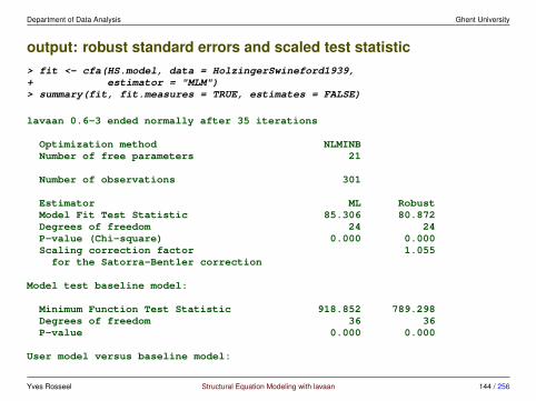
Department of Data Analysis Ghent University
output: robust standard errors and scaled test statistic> fit <- cfa(HS.model, data = HolzingerSwineford1939,+ estimator = "MLM")> summary(fit, fit.measures = TRUE, estimates = FALSE)
lavaan 0.6-3 ended normally after 35 iterations
Optimization method NLMINBNumber of free parameters 21
Number of observations 301
Estimator ML RobustModel Fit Test Statistic 85.306 80.872Degrees of freedom 24 24P-value (Chi-square) 0.000 0.000Scaling correction factor 1.055
for the Satorra-Bentler correction
Model test baseline model:
Minimum Function Test Statistic 918.852 789.298Degrees of freedom 36 36P-value 0.000 0.000
User model versus baseline model:
Yves Rosseel Structural Equation Modeling with lavaan 144 / 256
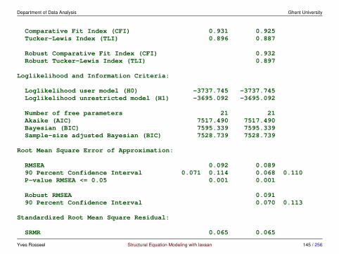
Department of Data Analysis Ghent University
Comparative Fit Index (CFI) 0.931 0.925Tucker-Lewis Index (TLI) 0.896 0.887
Robust Comparative Fit Index (CFI) 0.932Robust Tucker-Lewis Index (TLI) 0.897
Loglikelihood and Information Criteria:
Loglikelihood user model (H0) -3737.745 -3737.745Loglikelihood unrestricted model (H1) -3695.092 -3695.092
Number of free parameters 21 21Akaike (AIC) 7517.490 7517.490Bayesian (BIC) 7595.339 7595.339Sample-size adjusted Bayesian (BIC) 7528.739 7528.739
Root Mean Square Error of Approximation:
RMSEA 0.092 0.08990 Percent Confidence Interval 0.071 0.114 0.068 0.110P-value RMSEA <= 0.05 0.001 0.001
Robust RMSEA 0.09190 Percent Confidence Interval 0.070 0.113
Standardized Root Mean Square Residual:
SRMR 0.065 0.065
Yves Rosseel Structural Equation Modeling with lavaan 145 / 256
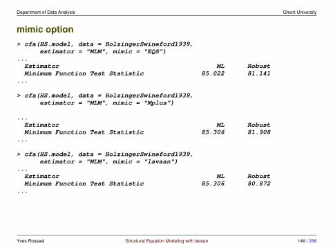
Department of Data Analysis Ghent University
mimic option> cfa(HS.model, data = HolzingerSwineford1939,
estimator = "MLM", mimic = "EQS")...Estimator ML RobustMinimum Function Test Statistic 85.022 81.141
...
> cfa(HS.model, data = HolzingerSwineford1939,estimator = "MLM", mimic = "Mplus")
...Estimator ML RobustMinimum Function Test Statistic 85.306 81.908
...
> cfa(HS.model, data = HolzingerSwineford1939,estimator = "MLM", mimic = "lavaan")
...Estimator ML RobustMinimum Function Test Statistic 85.306 80.872
...
Yves Rosseel Structural Equation Modeling with lavaan 146 / 256
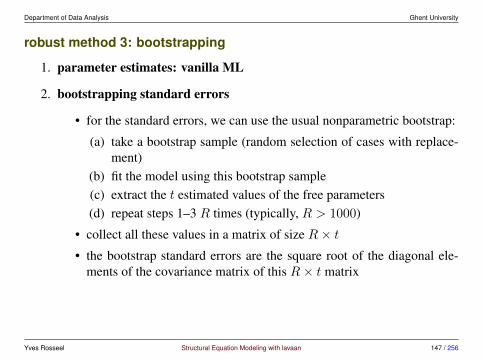
Department of Data Analysis Ghent University
robust method 3: bootstrapping
1. parameter estimates: vanilla ML
2. bootstrapping standard errors
• for the standard errors, we can use the usual nonparametric bootstrap:
(a) take a bootstrap sample (random selection of cases with replace-ment)
(b) fit the model using this bootstrap sample(c) extract the t estimated values of the free parameters(d) repeat steps 1–3 R times (typically, R > 1000)
• collect all these values in a matrix of size R× t• the bootstrap standard errors are the square root of the diagonal ele-
ments of the covariance matrix of this R× t matrix
Yves Rosseel Structural Equation Modeling with lavaan 147 / 256
Department of Data Analysis Ghent University
3. bootstrapping the test statistic
• for the test statistic, we can not use the usual nonparametric bootstrap,because it reflects not only non-normality and sampling variability, butalso model misfit
• the original sample must first be transformed so that the sample covari-ance matrix corresponds with the model-implied covariance matrix
• in the SEM literature, this model-based bootstrap procedure is knownas the Bollen-Stine bootstrap
• the standard p value of the chi-square test can be replaced by a boot-strap p value: the proportion of test statistics from the bootstrap sam-ples that exceed the value of the test statistic from the original (parent)sample
Yves Rosseel Structural Equation Modeling with lavaan 148 / 256

Department of Data Analysis Ghent University
bootstrapping in lavaan
• bootstrapping standard errors:
fit <- cfa(HS.model, data = HolzingerSwineford1939,se = "bootstrap", verbose = TRUE, bootstrap = 1000)
• bootstrapping the test statistic
fit <- cfa(HS.model, data = HolzingerSwineford1939,test = "bootstrap", verbose = TRUE, bootstrap = 1000)
• when we use se = ”bootstrap”, the parameterEstimates() output will containbootstrap based confidence intervals
Yves Rosseel Structural Equation Modeling with lavaan 149 / 256

Department of Data Analysis Ghent University
using bootstrapLavaan() to compute the Bollen-Stine p-value (optional)fit <- cfa(HS.model, data = HolzingerSwineford1939, se = "none")
# get the test statistic for the original sample
T.orig <- fitMeasures(fit, "chisq")
# bootstrap to get bootstrap test statistics# we only generate 10 bootstrap sample in this example; in practice# you may wish to use a much higher number
T.boot <- bootstrapLavaan(fit,R = 10,type = "bollen.stine",FUN = fitMeasures,fit.measures = "chisq")
# compute a bootstrap based p-value
pvalue.boot <- length(which(T.boot > T.orig))/length(T.boot)
Yves Rosseel Structural Equation Modeling with lavaan 150 / 256

Department of Data Analysis Ghent University
5 Categorical data
5.1 Handling categorical endogenous variablescategorical exogenous variables
• categorical exogenous covariates; eg. gender, country
• we simply need to construct ‘dummy variables’ and proceed as usual
• just like in ordinary regression
categorical endogenous variables
• need special treatment
• binary data, ordinal (ordered) data
• censored data, limited dependent data
• count data, nominal (unordered) data, . . .
Yves Rosseel Structural Equation Modeling with lavaan 151 / 256

Department of Data Analysis Ghent University
5.2 Two approaches for handling categorical data in a SEMframework
• limited information approach
– only univariate and bivariate information is used– estimation often proceeds in two or three stages; the first stages use
maximum likelihood, the last stage uses (weighted) least squares– mainly developed in the SEM literature– perhaps the best known implementation is in Mplus (WLSMV)
• full information approach
– all information is used– most practical: marginal maximum likelihood estimation– requires numerical integration (number of dimensions = number of la-
tent variables)– mainly developed in the IRT literature (and GLMM literature)– only recently incorporated in modern SEM software
Yves Rosseel Structural Equation Modeling with lavaan 152 / 256

Department of Data Analysis Ghent University
example SEM framework: u = binary, o = ordered, y = numeric
u1
u2
u3
u4
o1
o2
o3
o4
y1 y2 y3
f2
f3
f1
x1 x2
Yves Rosseel Structural Equation Modeling with lavaan 153 / 256
Department of Data Analysis Ghent University
full information approach
1. marginal maximum likelihood (MML)
2. latent response approach
3. Bayesian estimation
limited information approaches
1. three stage least squares (Mplus WLSMV)
2. pairwise likelihood estimation
Yves Rosseel Structural Equation Modeling with lavaan 154 / 256
Department of Data Analysis Ghent University
5.3 A limited information approach: the WLSMV estimator• developed by Bengt Muthen, in a series of papers; the seminal paper is
Muthen, B. (1984). A general structural equation model withdichotomous, ordered categorical, and continuous latent variableindicators. Psychometrika, 49, 115–132
• this approach has been the ‘golden standard’ in the SEM literature
• first available in LISCOMP (Linear Structural Equations using a Compre-hensive Measurement Model), distributed by SSI, 1987 – 1997
• follow up program: Mplus (Version 1: 1998), currently version 8
• other authors (Joreskog 1994; Lee, Poon, Bentler 1992) have proposed sim-ilar approaches (implemented in LISREL and EQS respectively)
• another great program: MECOSA (Arminger, G., Wittenberg, J., Schepers,A.) written in the GAUSS language (mid 90’s)
Yves Rosseel Structural Equation Modeling with lavaan 155 / 256
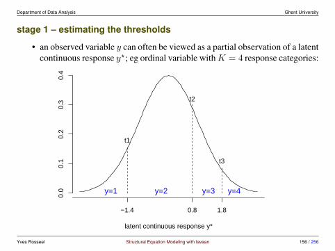
Department of Data Analysis Ghent University
stage 1 – estimating the thresholds
• an observed variable y can often be viewed as a partial observation of a latentcontinuous response y?; eg ordinal variable withK = 4 response categories:
latent continuous response y*
−1.4 0.8 1.8
0.0
0.1
0.2
0.3
0.4
y=1 y=2 y=3 y=4
t1
t2
t3
Yves Rosseel Structural Equation Modeling with lavaan 156 / 256

Department of Data Analysis Ghent University
stage 1 – estimating the thresholds in R
• if no exogenous variables, this is just
> set.seed(1234)> # generate `ordered' data with 4 categories> Y <- sample(1:4, size = 100, replace = TRUE)> # construct table of proportions> prop <- table(Y)/sum(table(Y))> prop
Y1 2 3 4
0.19 0.29 0.23 0.29
> # cumulative proportions> cprop <- c(0, cumsum(prop))> cprop
1 2 3 40.00 0.19 0.48 0.71 1.00
> # convert quantiles to z-scores> th <- qnorm(cprop)> th
Yves Rosseel Structural Equation Modeling with lavaan 157 / 256
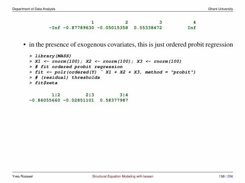
Department of Data Analysis Ghent University
1 2 3 4-Inf -0.87789630 -0.05015358 0.55338472 Inf
• in the presence of exogenous covariates, this is just ordered probit regression
> library(MASS)> X1 <- rnorm(100); X2 <- rnorm(100); X3 <- rnorm(100)> # fit ordered probit regression> fit <- polr(ordered(Y) ˜ X1 + X2 + X3, method = "probit")> # (residual) thresholds> fit$zeta
1|2 2|3 3|4-0.86055660 -0.02851101 0.58377987
Yves Rosseel Structural Equation Modeling with lavaan 158 / 256
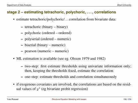
Department of Data Analysis Ghent University
stage 2 – estimating tetrachoric, polychoric, . . . , correlations
• estimate tetrachoric/polychoric/. . . correlation from bivariate data:
– tetrachoric (binary – binary)
– polychoric (ordered – ordered)
– polyserial (ordered – numeric)
– biserial (binary – numeric)
– pearson (numeric – numeric)
• ML estimation is available (see eg. Olsson 1979 and 1982)
– two-step: first estimate thresholds using univariate information only;then, keeping the thresholds fixed, estimate the correlation
– one-step: estimate thresholds and correlation simultaneously
• if exogenous covariates are involved, the correlations are based on the resid-ual values of y? (eg bivariate probit regression)
Yves Rosseel Structural Equation Modeling with lavaan 159 / 256

Department of Data Analysis Ghent University
stage 2 – tetrachoric, polychoric, . . . , correlations in R
• lavaan provides the lavCor() function to compute the tetrachoric, poly-choric, polyserial, . . . correlations
• example using two binary variables:
> library(lavaan)> # create some random correlated data> set.seed(1234)> Y12 <- MASS:::mvrnorm(n = 100, mu = c(0,0),+ Sigma = matrix(c(1,0.5,0.5,1), 2, 2))> # transform to binary> y1 <- cut(Y12[,1], breaks = c(-Inf, 0, +Inf), labels = FALSE)> y2 <- cut(Y12[,2], breaks = c(-Inf, 0, +Inf), labels = FALSE)> Data <- data.frame(y1 = y1, y2 = y2)
> # compute tetrachoric correlation> lavCor(Data, ordered = c("y1", "y2"))
y1 y2y1 1.000y2 0.713 1.000
Yves Rosseel Structural Equation Modeling with lavaan 160 / 256

Department of Data Analysis Ghent University
stage 2b – estimating the W matrix
• in the ideal case, W reflects the (asymptotic) variance matrix of the samplestatistics: the thresholds and the correlations
• an estimate of (N times) this variance matrix can be computed as follows:> fit <- sem('y1 ˜˜ y2', data = Data, ordered = c("y1", "y2"),+ estimator = "WLS")> lavInspect(fit, "Gamma")
[,1] [,2] [,3][1,] 1.658[2,] 0.809 1.601[3,] -0.070 -0.015 0.960
• the first two rows/columns correspond to the two thresholds; the last row/columncorresponds to the single tetrachoric correlation
• the diagonal elements reflect the variances of these statistics (over repeatedsampling)
• th off-diagonal elements reflect the covariances of these statistics (over re-peated sampling)
Yves Rosseel Structural Equation Modeling with lavaan 161 / 256

Department of Data Analysis Ghent University
stage 3 – estimating the SEM model
• third stage uses weighted least squares:
FWLS = (s− σ)>W−1(s− σ)
where s and σ are vectors containing all relevant sample-based and model-based statistics respectively
• s contains: thresholds, correlations, optionally regression slopes of exoge-nous covariates, optionally variances and means of continuous variables
• the weight matrix W is (a consistent estimator of) the asymptotic covariancematrix of the sample statistics (s)
• robust version: WLSMV
– use the diagonal of W only for estimation (DWLS)– use the full matrix for inference (standard errors and test statistic)– ‘MV’ stands for the Satterthwaite’s mean and variance corrected test
statistic
Yves Rosseel Structural Equation Modeling with lavaan 162 / 256

Department of Data Analysis Ghent University
alternative estimators, standard errors, and test statistics
• in the weighted least squares framework, we can choose between three dif-ferent choises for W, leading to three different estimators:
– estimator WLS: the full weight matrix W is used during estimation– estimator DWLS: only the diagonal of W is used during estimation– estimator ULS: W is replaced by the identity matrix (I)
• two common types of standard errors:
– ‘classic’ standard errors (based on the information matrix only)– ‘robust’ standard errors (using a sandwich type approach)
• four test statistics:
– uncorrected, standard chi-square test statistic– mean adjusted test statistic (Satorra-Bentler type)– mean and variance adjusted test statistic (Satterthwaite type)– scaled and shifted test statistic (new in Mplus 6)
Yves Rosseel Structural Equation Modeling with lavaan 163 / 256

Department of Data Analysis Ghent University
the Mplus legacy (optional)
• in Mplus, the ‘default’ estimator (for models with endogenous categoricalvariables) is termed WLSMV
• the term ‘WLSMV’ is widely used in the SEM literature
• in version 1 up to version 5 of Mplus, estimator WLSMV implies:
– diagonally weighted least-squares estimation (DWLS)
– robust standard errors
– a mean and variance adjusted test statistic (hence, the MV extension)
• other available estimators (in Mplus) are
– WLS (classical WLS, full weight matrix, classic standard errors andtest statistic)
– WLSM (DWLS + robust standard errors + mean-adjusted test statistic)
– ULS, USLM and ULSMV (the latter two use the full weight matrix forcomputing standard errors and adjusted test statistics)
Yves Rosseel Structural Equation Modeling with lavaan 164 / 256

Department of Data Analysis Ghent University
• since Mplus 6 (April 2010), the mean and variance adjusted test statistic wasreplaced by a ‘scaled and shifted’ test statistic
– they still call this WLSMV
– no need to adjust the degrees of freedom, so interpretation is easier
– to get the ‘old’ behaviour, you need to set the ‘satterthwaite=on’ option
Yves Rosseel Structural Equation Modeling with lavaan 165 / 256
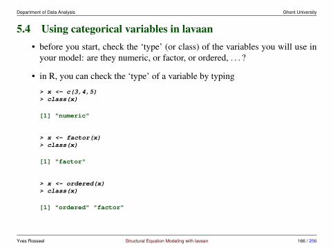
Department of Data Analysis Ghent University
5.4 Using categorical variables in lavaan• before you start, check the ‘type’ (or class) of the variables you will use in
your model: are they numeric, or factor, or ordered, . . . ?
• in R, you can check the ‘type’ of a variable by typing
> x <- c(3,4,5)> class(x)
[1] "numeric"
> x <- factor(x)> class(x)
[1] "factor"
> x <- ordered(x)> class(x)
[1] "ordered" "factor"
Yves Rosseel Structural Equation Modeling with lavaan 166 / 256
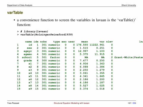
Department of Data Analysis Ghent University
varTable
• a convenience function to screen the variables in lavaan is the ‘varTable()’function:
> # library(lavaan)> varTable(HolzingerSwineford1939)
name idx nobs type exo user mean var nlev lnam1 id 1 301 numeric 0 0 176.555 11222.961 02 sex 2 301 numeric 0 0 1.515 0.251 03 ageyr 3 301 numeric 0 0 12.997 1.103 04 agemo 4 301 numeric 0 0 5.375 11.915 05 school 5 301 factor 0 0 NA NA 2 Grant-White|Pasteur6 grade 6 300 numeric 0 0 7.477 0.250 07 x1 7 301 numeric 0 0 4.936 1.363 08 x2 8 301 numeric 0 0 6.088 1.386 09 x3 9 301 numeric 0 0 2.250 1.279 010 x4 10 301 numeric 0 0 3.061 1.355 011 x5 11 301 numeric 0 0 4.341 1.665 012 x6 12 301 numeric 0 0 2.186 1.200 013 x7 13 301 numeric 0 0 4.186 1.187 014 x8 14 301 numeric 0 0 5.527 1.025 015 x9 15 301 numeric 0 0 5.374 1.018 0
Yves Rosseel Structural Equation Modeling with lavaan 167 / 256
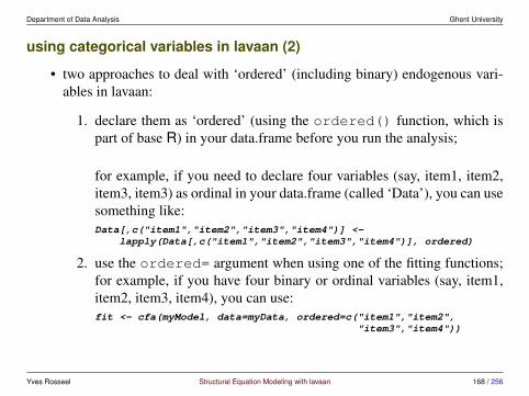
Department of Data Analysis Ghent University
using categorical variables in lavaan (2)
• two approaches to deal with ‘ordered’ (including binary) endogenous vari-ables in lavaan:
1. declare them as ‘ordered’ (using the ordered() function, which ispart of base R) in your data.frame before you run the analysis;
for example, if you need to declare four variables (say, item1, item2,item3, item3) as ordinal in your data.frame (called ‘Data’), you can usesomething like:Data[,c("item1","item2","item3","item4")] <-
lapply(Data[,c("item1","item2","item3","item4")], ordered)
2. use the ordered= argument when using one of the fitting functions;for example, if you have four binary or ordinal variables (say, item1,item2, item3, item4), you can use:fit <- cfa(myModel, data=myData, ordered=c("item1","item2",
"item3","item4"))
Yves Rosseel Structural Equation Modeling with lavaan 168 / 256
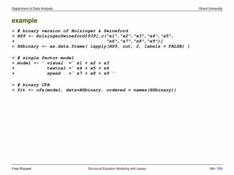
Department of Data Analysis Ghent University
example> # binary version of Holzinger & Swineford> HS9 <- HolzingerSwineford1939[,c("x1","x2","x3","x4","x5",+ "x6","x7","x8","x9")]> HSbinary <- as.data.frame( lapply(HS9, cut, 2, labels = FALSE) )
> # single factor model> model <- ' visual =˜ x1 + x2 + x3+ textual =˜ x4 + x5 + x6+ speed =˜ x7 + x8 + x9 '
> # binary CFA> fit <- cfa(model, data=HSbinary, ordered = names(HSbinary))
Yves Rosseel Structural Equation Modeling with lavaan 169 / 256
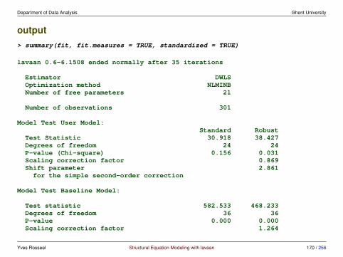
Department of Data Analysis Ghent University
output> summary(fit, fit.measures = TRUE, standardized = TRUE)
lavaan 0.6-6.1508 ended normally after 35 iterations
Estimator DWLSOptimization method NLMINBNumber of free parameters 21
Number of observations 301
Model Test User Model:Standard Robust
Test Statistic 30.918 38.427Degrees of freedom 24 24P-value (Chi-square) 0.156 0.031Scaling correction factor 0.869Shift parameter 2.861for the simple second-order correction
Model Test Baseline Model:
Test statistic 582.533 468.233Degrees of freedom 36 36P-value 0.000 0.000Scaling correction factor 1.264
Yves Rosseel Structural Equation Modeling with lavaan 170 / 256

Department of Data Analysis Ghent University
User Model versus Baseline Model:
Comparative Fit Index (CFI) 0.987 0.967Tucker-Lewis Index (TLI) 0.981 0.950
Robust Comparative Fit Index (CFI) NARobust Tucker-Lewis Index (TLI) NA
Root Mean Square Error of Approximation:
RMSEA 0.031 0.04590 Percent confidence interval - lower 0.000 0.01490 Percent confidence interval - upper 0.059 0.070P-value RMSEA <= 0.05 0.847 0.600
Robust RMSEA NA90 Percent confidence interval - lower NA90 Percent confidence interval - upper NA
Standardized Root Mean Square Residual:
SRMR 0.083 0.083
Parameter Estimates:
Information ExpectedInformation saturated (h1) model UnstructuredStandard errors Robust.sem
Yves Rosseel Structural Equation Modeling with lavaan 171 / 256

Department of Data Analysis Ghent University
Latent Variables:Estimate Std.Err z-value P(>|z|) Std.lv Std.all
visual =˜x1 1.000 0.639 0.639x2 0.900 0.188 4.788 0.000 0.575 0.575x3 0.939 0.197 4.766 0.000 0.600 0.600
textual =˜x4 1.000 0.835 0.835x5 0.976 0.118 8.241 0.000 0.815 0.815x6 1.078 0.125 8.601 0.000 0.900 0.900
speed =˜x7 1.000 0.471 0.471x8 1.569 0.461 3.403 0.001 0.740 0.740x9 1.449 0.409 3.541 0.000 0.683 0.683
Covariances:Estimate Std.Err z-value P(>|z|) Std.lv Std.all
visual ˜˜textual 0.303 0.061 4.981 0.000 0.569 0.569speed 0.132 0.049 2.700 0.007 0.439 0.439
textual ˜˜speed 0.076 0.046 1.656 0.098 0.192 0.192
Intercepts:Estimate Std.Err z-value P(>|z|) Std.lv Std.all
.x1 0.000 0.000 0.000
.x2 0.000 0.000 0.000
Yves Rosseel Structural Equation Modeling with lavaan 172 / 256
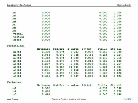
Department of Data Analysis Ghent University
.x3 0.000 0.000 0.000
.x4 0.000 0.000 0.000
.x5 0.000 0.000 0.000
.x6 0.000 0.000 0.000
.x7 0.000 0.000 0.000
.x8 0.000 0.000 0.000
.x9 0.000 0.000 0.000visual 0.000 0.000 0.000textual 0.000 0.000 0.000speed 0.000 0.000 0.000
Thresholds:Estimate Std.Err z-value P(>|z|) Std.lv Std.all
x1|t1 -0.388 0.074 -5.223 0.000 -0.388 -0.388x2|t1 -0.054 0.072 -0.748 0.454 -0.054 -0.054x3|t1 0.318 0.074 4.309 0.000 0.318 0.318x4|t1 0.180 0.073 2.473 0.013 0.180 0.180x5|t1 -0.257 0.073 -3.506 0.000 -0.257 -0.257x6|t1 1.024 0.088 11.641 0.000 1.024 1.024x7|t1 0.231 0.073 3.162 0.002 0.231 0.231x8|t1 1.128 0.092 12.284 0.000 1.128 1.128x9|t1 0.626 0.078 8.047 0.000 0.626 0.626
Variances:Estimate Std.Err z-value P(>|z|) Std.lv Std.all
.x1 0.592 0.592 0.592
.x2 0.670 0.670 0.670
.x3 0.640 0.640 0.640
Yves Rosseel Structural Equation Modeling with lavaan 173 / 256
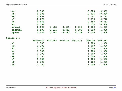
Department of Data Analysis Ghent University
.x4 0.303 0.303 0.303
.x5 0.336 0.336 0.336
.x6 0.191 0.191 0.191
.x7 0.778 0.778 0.778
.x8 0.453 0.453 0.453
.x9 0.534 0.534 0.534visual 0.408 0.112 3.651 0.000 1.000 1.000textual 0.697 0.101 6.883 0.000 1.000 1.000speed 0.222 0.094 2.363 0.018 1.000 1.000
Scales y*:Estimate Std.Err z-value P(>|z|) Std.lv Std.all
x1 1.000 1.000 1.000x2 1.000 1.000 1.000x3 1.000 1.000 1.000x4 1.000 1.000 1.000x5 1.000 1.000 1.000x6 1.000 1.000 1.000x7 1.000 1.000 1.000x8 1.000 1.000 1.000x9 1.000 1.000 1.000
Yves Rosseel Structural Equation Modeling with lavaan 174 / 256
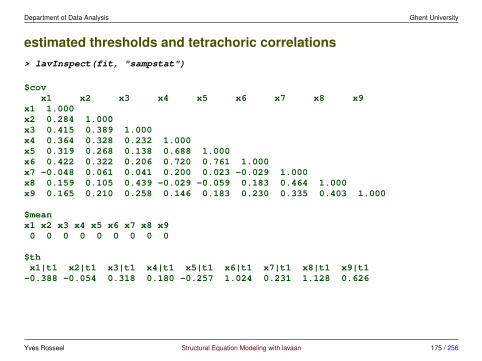
Department of Data Analysis Ghent University
estimated thresholds and tetrachoric correlations> lavInspect(fit, "sampstat")
$covx1 x2 x3 x4 x5 x6 x7 x8 x9
x1 1.000x2 0.284 1.000x3 0.415 0.389 1.000x4 0.364 0.328 0.232 1.000x5 0.319 0.268 0.138 0.688 1.000x6 0.422 0.322 0.206 0.720 0.761 1.000x7 -0.048 0.061 0.041 0.200 0.023 -0.029 1.000x8 0.159 0.105 0.439 -0.029 -0.059 0.183 0.464 1.000x9 0.165 0.210 0.258 0.146 0.183 0.230 0.335 0.403 1.000
$meanx1 x2 x3 x4 x5 x6 x7 x8 x90 0 0 0 0 0 0 0 0
$thx1|t1 x2|t1 x3|t1 x4|t1 x5|t1 x6|t1 x7|t1 x8|t1 x9|t1-0.388 -0.054 0.318 0.180 -0.257 1.024 0.231 1.128 0.626
Yves Rosseel Structural Equation Modeling with lavaan 175 / 256

Department of Data Analysis Ghent University
estimators, standard errors and test statistics in lavaan
• in lavaan, you can set your estimator, type of standard errors, and type oftest statistic separately
• estimators (least squares framework):
– estimator="WLS"
– estimator="DWLS"
– estimator="ULS"
• standard errors:
– se="standard"
– se="robust"
– se="bootstrap"
• test statistics:
– test="standard"
Yves Rosseel Structural Equation Modeling with lavaan 176 / 256

Department of Data Analysis Ghent University
– test="Satorra.Bentler"
– test="Satterthwaite"
– test="scaled.shifted"
– test="bootstrap or test="Bollen.Stine"
• or you can use the Mplus style shortcuts
• estimator="WLSMV" implies
– estimator="DWLS"
– se="robust"
– test="scaled.shifted" (following Mplus 6 and higher)
• estimator="WLSMVS" implies
– estimator="DWLS"
– se="robust"
– test="Satterthwaite" (following older versions of Mplus)
Yves Rosseel Structural Equation Modeling with lavaan 177 / 256

Department of Data Analysis Ghent University
• alternatives:
– estimator="WLSM"
– estimator="ULSMV"
– estimator="ULSM"
Yves Rosseel Structural Equation Modeling with lavaan 178 / 256
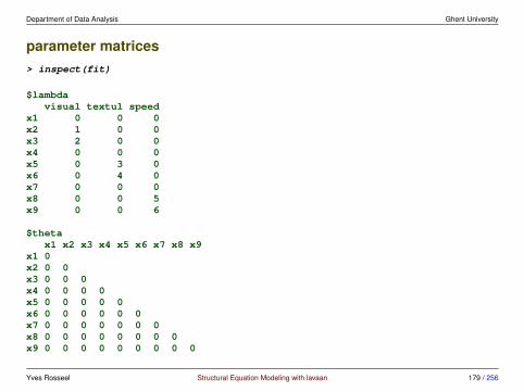
Department of Data Analysis Ghent University
parameter matrices> inspect(fit)
$lambdavisual textul speed
x1 0 0 0x2 1 0 0x3 2 0 0x4 0 0 0x5 0 3 0x6 0 4 0x7 0 0 0x8 0 0 5x9 0 0 6
$thetax1 x2 x3 x4 x5 x6 x7 x8 x9
x1 0x2 0 0x3 0 0 0x4 0 0 0 0x5 0 0 0 0 0x6 0 0 0 0 0 0x7 0 0 0 0 0 0 0x8 0 0 0 0 0 0 0 0x9 0 0 0 0 0 0 0 0 0
Yves Rosseel Structural Equation Modeling with lavaan 179 / 256
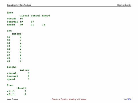
Department of Data Analysis Ghent University
$psivisual textul speed
visual 16textual 19 17speed 20 21 18
$nuintrcp
x1 0x2 0x3 0x4 0x5 0x6 0x7 0x8 0x9 0
$alphaintrcp
visual 0textual 0speed 0
$tauthrshl
x1|t1 7x2|t1 8
Yves Rosseel Structural Equation Modeling with lavaan 180 / 256

Department of Data Analysis Ghent University
x3|t1 9x4|t1 10x5|t1 11x6|t1 12x7|t1 13x8|t1 14x9|t1 15
$deltascales
x1 0x2 0x3 0x4 0x5 0x6 0x7 0x8 0x9 0
Yves Rosseel Structural Equation Modeling with lavaan 181 / 256
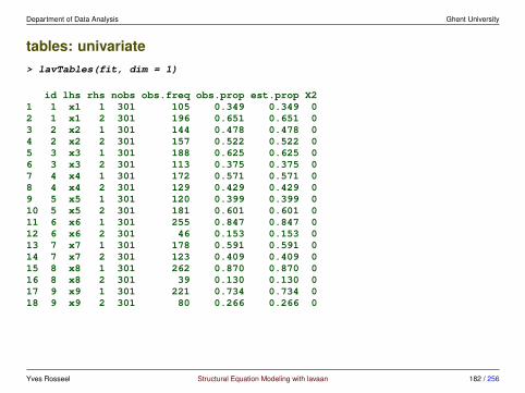
Department of Data Analysis Ghent University
tables: univariate> lavTables(fit, dim = 1)
id lhs rhs nobs obs.freq obs.prop est.prop X21 1 x1 1 301 105 0.349 0.349 02 1 x1 2 301 196 0.651 0.651 03 2 x2 1 301 144 0.478 0.478 04 2 x2 2 301 157 0.522 0.522 05 3 x3 1 301 188 0.625 0.625 06 3 x3 2 301 113 0.375 0.375 07 4 x4 1 301 172 0.571 0.571 08 4 x4 2 301 129 0.429 0.429 09 5 x5 1 301 120 0.399 0.399 010 5 x5 2 301 181 0.601 0.601 011 6 x6 1 301 255 0.847 0.847 012 6 x6 2 301 46 0.153 0.153 013 7 x7 1 301 178 0.591 0.591 014 7 x7 2 301 123 0.409 0.409 015 8 x8 1 301 262 0.870 0.870 016 8 x8 2 301 39 0.130 0.130 017 9 x9 1 301 221 0.734 0.734 018 9 x9 2 301 80 0.266 0.266 0
Yves Rosseel Structural Equation Modeling with lavaan 182 / 256
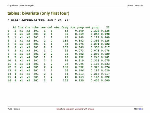
Department of Data Analysis Ghent University
tables: bivariate (only first four)> head( lavTables(fit, dim = 2), 16)
id lhs rhs nobs row col obs.freq obs.prop est.prop X21 1 x1 x2 301 1 1 63 0.209 0.222 0.2282 1 x1 x2 301 2 1 81 0.269 0.256 0.1983 1 x1 x2 301 1 2 42 0.140 0.127 0.4004 1 x1 x2 301 2 2 115 0.382 0.395 0.1285 2 x1 x3 301 1 1 83 0.276 0.271 0.0226 2 x1 x3 301 2 1 105 0.349 0.353 0.0177 2 x1 x3 301 1 2 22 0.073 0.078 0.0788 2 x1 x3 301 2 2 91 0.302 0.298 0.0209 3 x1 x4 301 1 1 76 0.252 0.243 0.10110 3 x1 x4 301 2 1 96 0.319 0.328 0.07511 3 x1 x4 301 1 2 29 0.096 0.105 0.23312 3 x1 x4 301 2 2 100 0.332 0.323 0.07613 4 x1 x5 301 1 1 56 0.186 0.183 0.02014 4 x1 x5 301 2 1 64 0.213 0.216 0.01715 4 x1 x5 301 1 2 49 0.163 0.166 0.02216 4 x1 x5 301 2 2 132 0.439 0.435 0.009
Yves Rosseel Structural Equation Modeling with lavaan 183 / 256

Department of Data Analysis Ghent University
5.5 SEM vs IRTthe connection with IRT
• the theoretical relationship between SEM and IRT has been well documented:
Takane, Y., & De Leeuw, J. (1987). On the relationship between itemresponse theory and factor analysis of discretized variables. Psychome-trika, 52, 393-408.Kamata, A., & Bauer, D. J. (2008). A note on the relation betweenfactor analytic and item response theory models. Structural EquationModeling, 15, 136-153.Joreskog, K. G., & Moustaki, I. (2001). Factor analysis of ordinal vari-ables: A comparison of three approaches. Multivariate Behavioral Re-search, 36, 347-387.
• IRT: focus is on the scale and the item characteristics, person scores
• SEM: focus is (often) on the structural relations among either observed orlatent variables; with or without exogenous covariates
• in lavaan (since 0.5-16): estimator="MML"
Yves Rosseel Structural Equation Modeling with lavaan 184 / 256
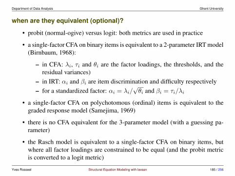
Department of Data Analysis Ghent University
when are they equivalent (optional)?
• probit (normal-ogive) versus logit: both metrics are used in practice
• a single-factor CFA on binary items is equivalent to a 2-parameter IRT model(Birnbaum, 1968):
– in CFA: λi, τi and θi are the factor loadings, the thresholds, and theresidual variances)
– in IRT: αi and βi are item discrimination and difficulty respectively– for a standardized factor: αi = λi/
√θi and βi = τi/λi
• a single-factor CFA on polychotomous (ordinal) items is equivalent to thegraded response model (Samejima, 1969)
• there is no CFA equivalent for the 3-parameter model (with a guessing pa-rameter)
• the Rasch model is equivalent to a single-factor CFA on binary items, butwhere all factor loadings are constrained to be equal (and the probit metricis converted to a logit metric)
Yves Rosseel Structural Equation Modeling with lavaan 185 / 256
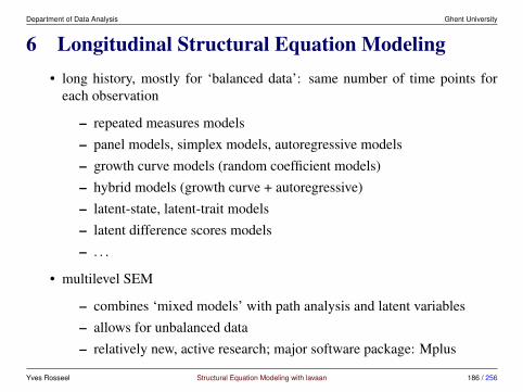
Department of Data Analysis Ghent University
6 Longitudinal Structural Equation Modeling• long history, mostly for ‘balanced data’: same number of time points for
each observation
– repeated measures models– panel models, simplex models, autoregressive models– growth curve models (random coefficient models)– hybrid models (growth curve + autoregressive)– latent-state, latent-trait models– latent difference scores models– . . .
• multilevel SEM
– combines ‘mixed models’ with path analysis and latent variables– allows for unbalanced data– relatively new, active research; major software package: Mplus
Yves Rosseel Structural Equation Modeling with lavaan 186 / 256

Department of Data Analysis Ghent University
Books
• Little, T. (2013). Longitudinal Structural Equation Modeling. Guilford Press
Yves Rosseel Structural Equation Modeling with lavaan 187 / 256

Department of Data Analysis Ghent University
• McArdle, J.J. and Nesselroade, J.R. (2014). Longitudinal Data AnalysisUsing Structural Equation Models. American Psychological Association(APA).
Yves Rosseel Structural Equation Modeling with lavaan 188 / 256

Department of Data Analysis Ghent University
• Bollen, K.A. and Curran, P.J. (2006). Latent Curve Models: A StructuralEquation Perspective. Wiley.
Yves Rosseel Structural Equation Modeling with lavaan 189 / 256
Department of Data Analysis Ghent University
6.1 Repeated measures ANOVA in SEM• we can mimic the classical repeated measures ANOVA in a SEM framework
• using two time-points only, this is the SEM equivalent of the paired t-test
• but we can relax the compound symmetry restriction
– we can allow for an unstructured covariance structure
– or we could impose an autoregressive AR(1) structure
– . . .
• but above all, we can replace the observed variables by latent variables
Yves Rosseel Structural Equation Modeling with lavaan 190 / 256
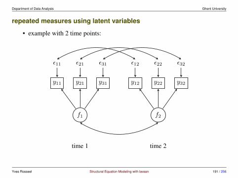
Department of Data Analysis Ghent University
repeated measures using latent variables
• example with 2 time points:
y11 y21 y31 y12 y22 y32
ε11 ε21 ε31 ε12 ε22 ε32
f1 f2
time 1 time 2
Yves Rosseel Structural Equation Modeling with lavaan 191 / 256

Department of Data Analysis Ghent University
comments
• first of all, we need to establish measurement invariance across time points
– it is tempting to do this using a multiple group analysis, using the timepoints as group levels, but this will not allow us to specify correlatedresiduals among the corresponding variables (and the time points arenot independent)
– therefore, we need to use labels for the different time points (for factorloadings and intercepts of observed variables), and impose the equalityconstraints by using the same label for the different time points
• since we wish to compare the latent means, we need ‘strong invariance’:
– equal factor loadings
– equal intercepts/means of the observed variables
• usually, we allow the residuals variances of the corresponding variablesacross time to be correlated
Yves Rosseel Structural Equation Modeling with lavaan 192 / 256
Department of Data Analysis Ghent University
• if we have more than two time points, we can allow for all possible correla-tions among the repeated latent variables (this corresponds to the ‘unstruc-tured’ assumption)
• the latent mean/intercept of the first time point is fixed to zero, while we esti-mate the latent mean/intercept of the other time points (although alternativecoding schemes are possible)
Yves Rosseel Structural Equation Modeling with lavaan 193 / 256

Department of Data Analysis Ghent University
real-world example
• example from Todd Little’s book (Longitudinal SEM, 2013): table 3.8 andfigure 3.10 (but with equality constraints)
• the latent variable ‘positive affect’ is measured by three indicators (Glad,Cheerful and Happy): 823 children in grades 7 en 8 responded to questionslike “In the past 2 weeks, I have felt . . . ” (with 4 response categories: almostnever, seldom, often, almost always)
• measured at two time points: in the fall of two successive school years
• main question: is there a significant difference in (self-reported) ‘positiveaffect’ between the two time points?
• this is the SEM equivalent of the paired t-test
Yves Rosseel Structural Equation Modeling with lavaan 194 / 256
Department of Data Analysis Ghent University
caveats
• we have no access to the full data, but the tables in the book report all thesample statistics we need (means, standard deviations, correlations, samplesize)
• we will have to convert the correlations to covariances (using the standarddeviations); lavaan has a convenience function getCov() for doing justthat
• before we attempt to compare two latent means, we must first establish mea-surement invariance (over time)
Yves Rosseel Structural Equation Modeling with lavaan 195 / 256
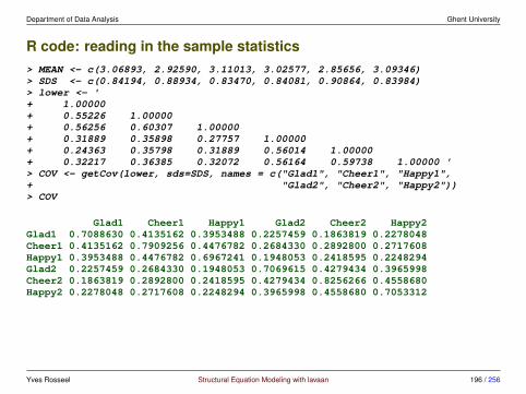
Department of Data Analysis Ghent University
R code: reading in the sample statistics> MEAN <- c(3.06893, 2.92590, 3.11013, 3.02577, 2.85656, 3.09346)> SDS <- c(0.84194, 0.88934, 0.83470, 0.84081, 0.90864, 0.83984)> lower <- '+ 1.00000+ 0.55226 1.00000+ 0.56256 0.60307 1.00000+ 0.31889 0.35898 0.27757 1.00000+ 0.24363 0.35798 0.31889 0.56014 1.00000+ 0.32217 0.36385 0.32072 0.56164 0.59738 1.00000 '> COV <- getCov(lower, sds=SDS, names = c("Glad1", "Cheer1", "Happy1",+ "Glad2", "Cheer2", "Happy2"))> COV
Glad1 Cheer1 Happy1 Glad2 Cheer2 Happy2Glad1 0.7088630 0.4135162 0.3953488 0.2257459 0.1863819 0.2278048Cheer1 0.4135162 0.7909256 0.4476782 0.2684330 0.2892800 0.2717608Happy1 0.3953488 0.4476782 0.6967241 0.1948053 0.2418595 0.2248294Glad2 0.2257459 0.2684330 0.1948053 0.7069615 0.4279434 0.3965998Cheer2 0.1863819 0.2892800 0.2418595 0.4279434 0.8256266 0.4558680Happy2 0.2278048 0.2717608 0.2248294 0.3965998 0.4558680 0.7053312
Yves Rosseel Structural Equation Modeling with lavaan 196 / 256
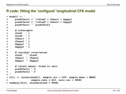
Department of Data Analysis Ghent University
R code: fitting the ‘configural’ longitudinal CFA model> model1 <- '+ posAffect1 =˜ 1*Glad1 + Cheer1 + Happy1+ posAffect2 =˜ 1*Glad2 + Cheer2 + Happy2+ posAffect1 ˜˜ posAffect2++ # intercepts+ Glad1 ˜ 1+ Glad2 ˜ 1+ Cheer1 ˜ 1+ Cheer2 ˜ 1+ Happy1 ˜ 1+ Happy2 ˜ 1++ # residual covariances+ Glad1 ˜˜ Glad2+ Cheer1 ˜˜ Cheer2+ Happy1 ˜˜ Happy2++ # latent means: fixed to zero+ posAffect1 ˜ 0+ posAffect2 ˜ 0+ '> fit1 <- lavaan(model1, sample.cov = COV, sample.mean = MEAN,+ sample.nobs = 823, auto.var = TRUE)> summary(fit1, standardized = TRUE)
Yves Rosseel Structural Equation Modeling with lavaan 197 / 256
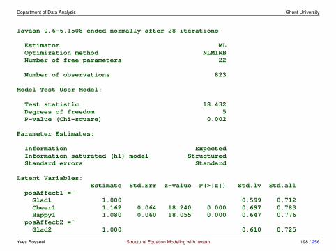
Department of Data Analysis Ghent University
lavaan 0.6-6.1508 ended normally after 28 iterations
Estimator MLOptimization method NLMINBNumber of free parameters 22
Number of observations 823
Model Test User Model:
Test statistic 18.432Degrees of freedom 5P-value (Chi-square) 0.002
Parameter Estimates:
Information ExpectedInformation saturated (h1) model StructuredStandard errors Standard
Latent Variables:Estimate Std.Err z-value P(>|z|) Std.lv Std.all
posAffect1 =˜Glad1 1.000 0.599 0.712Cheer1 1.162 0.064 18.240 0.000 0.697 0.783Happy1 1.080 0.060 18.055 0.000 0.647 0.776
posAffect2 =˜Glad2 1.000 0.610 0.725
Yves Rosseel Structural Equation Modeling with lavaan 198 / 256

Department of Data Analysis Ghent University
Cheer2 1.136 0.062 18.247 0.000 0.693 0.764Happy2 1.075 0.059 18.249 0.000 0.656 0.782
Covariances:Estimate Std.Err z-value P(>|z|) Std.lv Std.all
posAffect1 ˜˜posAffect2 0.202 0.021 9.840 0.000 0.553 0.553
.Glad1 ˜˜.Glad2 0.031 0.015 2.055 0.040 0.031 0.092
.Cheer1 ˜˜.Cheer2 0.018 0.016 1.076 0.282 0.018 0.055
.Happy1 ˜˜.Happy2 -0.011 0.014 -0.767 0.443 -0.011 -0.039
Intercepts:Estimate Std.Err z-value P(>|z|) Std.lv Std.all
.Glad1 3.069 0.029 104.641 0.000 3.069 3.648
.Glad2 3.026 0.029 103.189 0.000 3.026 3.597
.Cheer1 2.926 0.031 94.378 0.000 2.926 3.290
.Cheer2 2.857 0.032 90.334 0.000 2.857 3.149
.Happy1 3.110 0.029 106.913 0.000 3.110 3.727
.Happy2 3.093 0.029 105.772 0.000 3.093 3.687posAffect1 0.000 0.000 0.000posAffect2 0.000 0.000 0.000
Variances:Estimate Std.Err z-value P(>|z|) Std.lv Std.all
.Glad1 0.349 0.023 15.214 0.000 0.349 0.492
Yves Rosseel Structural Equation Modeling with lavaan 199 / 256
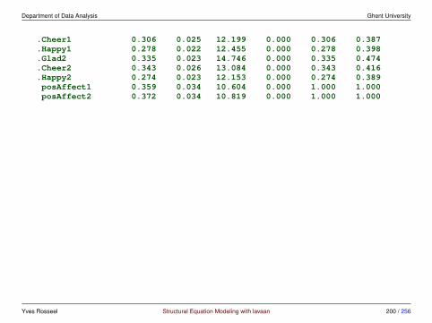
Department of Data Analysis Ghent University
.Cheer1 0.306 0.025 12.199 0.000 0.306 0.387
.Happy1 0.278 0.022 12.455 0.000 0.278 0.398
.Glad2 0.335 0.023 14.746 0.000 0.335 0.474
.Cheer2 0.343 0.026 13.084 0.000 0.343 0.416
.Happy2 0.274 0.023 12.153 0.000 0.274 0.389posAffect1 0.359 0.034 10.604 0.000 1.000 1.000posAffect2 0.372 0.034 10.819 0.000 1.000 1.000
Yves Rosseel Structural Equation Modeling with lavaan 200 / 256

Department of Data Analysis Ghent University
R code: fitting the ‘weak invariance’ longitudinal CFA model> model2 <- '+ posAffect1 =˜ 1*Glad1 + ch*Cheer1 + ha*Happy1+ posAffect2 =˜ 1*Glad2 + ch*Cheer2 + ha*Happy2+ posAffect1 ˜˜ posAffect2++ # intercepts+ Glad1 ˜ 1+ Glad2 ˜ 1+ Cheer1 ˜ 1+ Cheer2 ˜ 1+ Happy1 ˜ 1+ Happy2 ˜ 1++ # residual covariances+ Glad1 ˜˜ Glad2+ Cheer1 ˜˜ Cheer2+ Happy1 ˜˜ Happy2++ # latent means: fixed to zero+ posAffect1 ˜ 0+ posAffect2 ˜ 0+ '> fit2 <- lavaan(model2, sample.cov = COV, sample.mean = MEAN,+ sample.nobs = 823, auto.var = TRUE)> summary(fit2, standardized = TRUE)
Yves Rosseel Structural Equation Modeling with lavaan 201 / 256
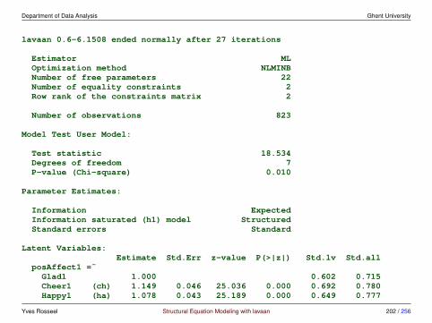
Department of Data Analysis Ghent University
lavaan 0.6-6.1508 ended normally after 27 iterations
Estimator MLOptimization method NLMINBNumber of free parameters 22Number of equality constraints 2Row rank of the constraints matrix 2
Number of observations 823
Model Test User Model:
Test statistic 18.534Degrees of freedom 7P-value (Chi-square) 0.010
Parameter Estimates:
Information ExpectedInformation saturated (h1) model StructuredStandard errors Standard
Latent Variables:Estimate Std.Err z-value P(>|z|) Std.lv Std.all
posAffect1 =˜Glad1 1.000 0.602 0.715Cheer1 (ch) 1.149 0.046 25.036 0.000 0.692 0.780Happy1 (ha) 1.078 0.043 25.189 0.000 0.649 0.777
Yves Rosseel Structural Equation Modeling with lavaan 202 / 256
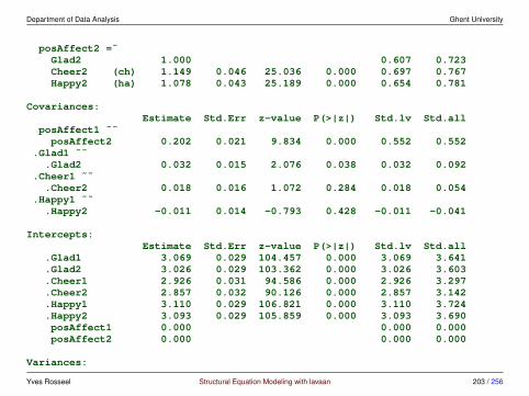
Department of Data Analysis Ghent University
posAffect2 =˜Glad2 1.000 0.607 0.723Cheer2 (ch) 1.149 0.046 25.036 0.000 0.697 0.767Happy2 (ha) 1.078 0.043 25.189 0.000 0.654 0.781
Covariances:Estimate Std.Err z-value P(>|z|) Std.lv Std.all
posAffect1 ˜˜posAffect2 0.202 0.021 9.834 0.000 0.552 0.552
.Glad1 ˜˜.Glad2 0.032 0.015 2.076 0.038 0.032 0.092
.Cheer1 ˜˜.Cheer2 0.018 0.016 1.072 0.284 0.018 0.054
.Happy1 ˜˜.Happy2 -0.011 0.014 -0.793 0.428 -0.011 -0.041
Intercepts:Estimate Std.Err z-value P(>|z|) Std.lv Std.all
.Glad1 3.069 0.029 104.457 0.000 3.069 3.641
.Glad2 3.026 0.029 103.362 0.000 3.026 3.603
.Cheer1 2.926 0.031 94.586 0.000 2.926 3.297
.Cheer2 2.857 0.032 90.126 0.000 2.857 3.142
.Happy1 3.110 0.029 106.821 0.000 3.110 3.724
.Happy2 3.093 0.029 105.859 0.000 3.093 3.690posAffect1 0.000 0.000 0.000posAffect2 0.000 0.000 0.000
Variances:
Yves Rosseel Structural Equation Modeling with lavaan 203 / 256
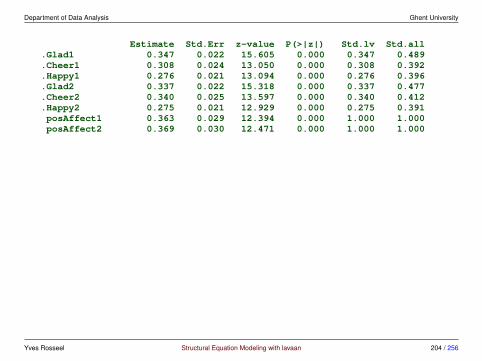
Department of Data Analysis Ghent University
Estimate Std.Err z-value P(>|z|) Std.lv Std.all.Glad1 0.347 0.022 15.605 0.000 0.347 0.489.Cheer1 0.308 0.024 13.050 0.000 0.308 0.392.Happy1 0.276 0.021 13.094 0.000 0.276 0.396.Glad2 0.337 0.022 15.318 0.000 0.337 0.477.Cheer2 0.340 0.025 13.597 0.000 0.340 0.412.Happy2 0.275 0.021 12.929 0.000 0.275 0.391posAffect1 0.363 0.029 12.394 0.000 1.000 1.000posAffect2 0.369 0.030 12.471 0.000 1.000 1.000
Yves Rosseel Structural Equation Modeling with lavaan 204 / 256

Department of Data Analysis Ghent University
R code: testing for weak invariance
• compare the configural and the weak invariance models:
> anova(fit1, fit2)
Chi-Squared Difference Test
Df AIC BIC Chisq Chisq diff Df diff Pr(>Chisq)fit1 5 10804 10908 18.432fit2 7 10800 10894 18.534 0.1019 2 0.9503
• good, we have weak invariance over time
Yves Rosseel Structural Equation Modeling with lavaan 205 / 256

Department of Data Analysis Ghent University
R code: fitting the ‘strong invariance’ longitudinal CFA model> model3 <- '+ posAffect1 =˜ 1*Glad1 + ch*Cheer1 + ha*Happy1+ posAffect2 =˜ 1*Glad2 + ch*Cheer2 + ha*Happy2+ posAffect1 ˜˜ posAffect2++ # intercepts+ Glad1 ˜ igl*1+ Glad2 ˜ igl*1+ Cheer1 ˜ ich*1+ Cheer2 ˜ ich*1+ Happy1 ˜ iha*1+ Happy2 ˜ iha*1++ # residual covariances+ Glad1 ˜˜ Glad2+ Cheer1 ˜˜ Cheer2+ Happy1 ˜˜ Happy2++ # latent means: fixed to zero+ posAffect1 ˜ 0*1 # baseline+ posAffect2 ˜ 1 # difference compared to baseline+ '> fit3 <- lavaan(model3, sample.cov = COV, sample.mean = MEAN,+ sample.nobs = 823, auto.var = TRUE)> summary(fit3, standardized = TRUE)
Yves Rosseel Structural Equation Modeling with lavaan 206 / 256
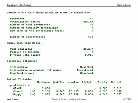
Department of Data Analysis Ghent University
lavaan 0.6-6.1508 ended normally after 36 iterations
Estimator MLOptimization method NLMINBNumber of free parameters 23Number of equality constraints 5Row rank of the constraints matrix 5
Number of observations 823
Model Test User Model:
Test statistic 20.279Degrees of freedom 9P-value (Chi-square) 0.016
Parameter Estimates:
Information ExpectedInformation saturated (h1) model StructuredStandard errors Standard
Latent Variables:Estimate Std.Err z-value P(>|z|) Std.lv Std.all
posAffect1 =˜Glad1 1.000 0.603 0.715Cheer1 (ch) 1.150 0.046 25.063 0.000 0.693 0.780Happy1 (ha) 1.076 0.043 25.208 0.000 0.648 0.777
Yves Rosseel Structural Equation Modeling with lavaan 207 / 256
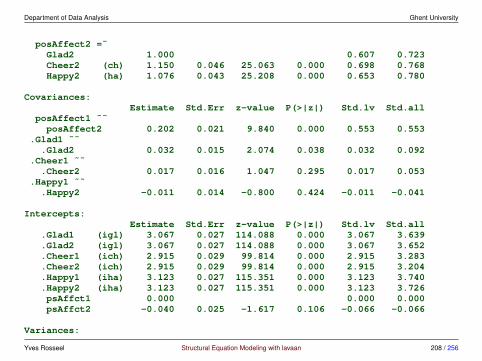
Department of Data Analysis Ghent University
posAffect2 =˜Glad2 1.000 0.607 0.723Cheer2 (ch) 1.150 0.046 25.063 0.000 0.698 0.768Happy2 (ha) 1.076 0.043 25.208 0.000 0.653 0.780
Covariances:Estimate Std.Err z-value P(>|z|) Std.lv Std.all
posAffect1 ˜˜posAffect2 0.202 0.021 9.840 0.000 0.553 0.553
.Glad1 ˜˜.Glad2 0.032 0.015 2.074 0.038 0.032 0.092
.Cheer1 ˜˜.Cheer2 0.017 0.016 1.047 0.295 0.017 0.053
.Happy1 ˜˜.Happy2 -0.011 0.014 -0.800 0.424 -0.011 -0.041
Intercepts:Estimate Std.Err z-value P(>|z|) Std.lv Std.all
.Glad1 (igl) 3.067 0.027 114.088 0.000 3.067 3.639
.Glad2 (igl) 3.067 0.027 114.088 0.000 3.067 3.652
.Cheer1 (ich) 2.915 0.029 99.814 0.000 2.915 3.283
.Cheer2 (ich) 2.915 0.029 99.814 0.000 2.915 3.204
.Happy1 (iha) 3.123 0.027 115.351 0.000 3.123 3.740
.Happy2 (iha) 3.123 0.027 115.351 0.000 3.123 3.726psAffct1 0.000 0.000 0.000psAffct2 -0.040 0.025 -1.617 0.106 -0.066 -0.066
Variances:
Yves Rosseel Structural Equation Modeling with lavaan 208 / 256

Department of Data Analysis Ghent University
Estimate Std.Err z-value P(>|z|) Std.lv Std.all.Glad1 0.347 0.022 15.601 0.000 0.347 0.489.Cheer1 0.308 0.024 13.028 0.000 0.308 0.391.Happy1 0.277 0.021 13.133 0.000 0.277 0.397.Glad2 0.336 0.022 15.312 0.000 0.336 0.477.Cheer2 0.340 0.025 13.578 0.000 0.340 0.411.Happy2 0.275 0.021 12.968 0.000 0.275 0.392posAffect1 0.363 0.029 12.399 0.000 1.000 1.000posAffect2 0.369 0.030 12.477 0.000 1.000 1.000
Yves Rosseel Structural Equation Modeling with lavaan 209 / 256

Department of Data Analysis Ghent University
R code: testing for strong invariance
• compare the weak and the strong invariance model:
> anova(fit2, fit3)
Chi-Squared Difference Test
Df AIC BIC Chisq Chisq diff Df diff Pr(>Chisq)fit2 7 10800 10894 18.534fit3 9 10798 10883 20.279 1.7451 2 0.4179
• splendid, we have strong invariance over time
Is there a difference between the two latent means?
• because there is only a single (latent) variable, we can immediately see theanswer in the output of model3
• in general, we would need to fit a ‘null’ model where we constrain the twolatent means to be equal; next, we compare these two models using anova()
Yves Rosseel Structural Equation Modeling with lavaan 210 / 256
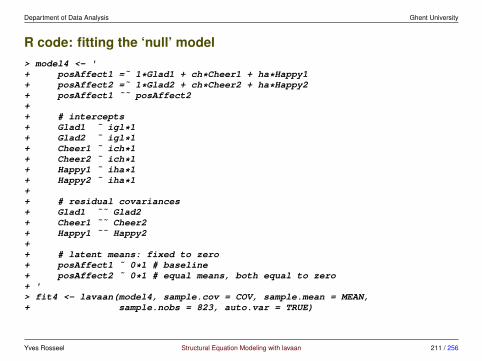
Department of Data Analysis Ghent University
R code: fitting the ‘null’ model> model4 <- '+ posAffect1 =˜ 1*Glad1 + ch*Cheer1 + ha*Happy1+ posAffect2 =˜ 1*Glad2 + ch*Cheer2 + ha*Happy2+ posAffect1 ˜˜ posAffect2++ # intercepts+ Glad1 ˜ igl*1+ Glad2 ˜ igl*1+ Cheer1 ˜ ich*1+ Cheer2 ˜ ich*1+ Happy1 ˜ iha*1+ Happy2 ˜ iha*1++ # residual covariances+ Glad1 ˜˜ Glad2+ Cheer1 ˜˜ Cheer2+ Happy1 ˜˜ Happy2++ # latent means: fixed to zero+ posAffect1 ˜ 0*1 # baseline+ posAffect2 ˜ 0*1 # equal means, both equal to zero+ '> fit4 <- lavaan(model4, sample.cov = COV, sample.mean = MEAN,+ sample.nobs = 823, auto.var = TRUE)
Yves Rosseel Structural Equation Modeling with lavaan 211 / 256
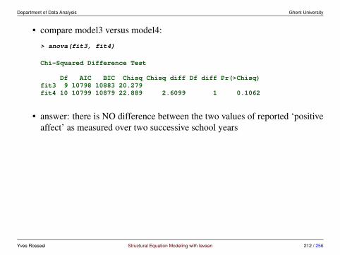
Department of Data Analysis Ghent University
• compare model3 versus model4:
> anova(fit3, fit4)
Chi-Squared Difference Test
Df AIC BIC Chisq Chisq diff Df diff Pr(>Chisq)fit3 9 10798 10883 20.279fit4 10 10799 10879 22.889 2.6099 1 0.1062
• answer: there is NO difference between the two values of reported ‘positiveaffect’ as measured over two successive school years
Yves Rosseel Structural Equation Modeling with lavaan 212 / 256
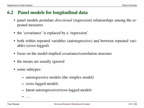
Department of Data Analysis Ghent University
6.2 Panel models for longitudinal data• panel models postulate directional (regression) relationships among the re-
peated measures
• the ‘covariance’ is replaced by a ‘regression’
• both within repeated variables (autoregressive) and between repeated vari-ables (cross-lagged)
• focus on the model-implied covariance/correlation structure
• the means are usually ignored
• some subtypes:
– autoregressive models (the simplex model)
– cross-lagged models
– latent autoregressive/cross-lagged models
– . . .
Yves Rosseel Structural Equation Modeling with lavaan 213 / 256
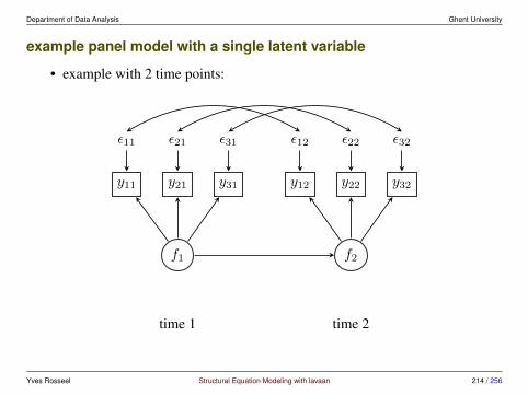
Department of Data Analysis Ghent University
example panel model with a single latent variable
• example with 2 time points:
y11 y21 y31 y12 y22 y32
ε11 ε21 ε31 ε12 ε22 ε32
f1 f2
time 1 time 2
Yves Rosseel Structural Equation Modeling with lavaan 214 / 256

Department of Data Analysis Ghent University
autoregressive models
• each time point is regressed on a previous time point (first order) , or an evenfurther time point (second order, third order, . . . )
• alternative names: Markov models, simplex models, panel models, . . .
• earliest development dates back to the seminal work of Guttman (1954)
• example first-order univariate autoregressive model:
y1 y2 y3 y4
ε2 ε3 ε4
? ? ?
Yves Rosseel Structural Equation Modeling with lavaan 215 / 256
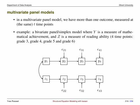
Department of Data Analysis Ghent University
multivariate panel models
• in a multivariate panel model, we have more than one outcome, measured at(the same) t time points
• example: a bivariate panel/simplex model where Y is a measure of mathe-matical achievement, and Z is a measure of reading ability (4 time points:grade 3, grade 4, grade 5 and grade 6)
y1 y2 y3 y4
z1 z2 z3 z4
ε21 ε31 ε41
ε22 ε32 ε43
Yves Rosseel Structural Equation Modeling with lavaan 216 / 256
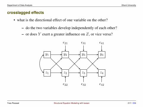
Department of Data Analysis Ghent University
crosslagged effects
• what is the directional effect of one variable on the other?
– do the two variables develop independently of each other?
– or does Y exert a greater influence on Z, or vice versa?
y1 y2 y3 y4
z1 z2 z3 z4
ε21 ε31 ε41
ε22 ε32 ε42
Yves Rosseel Structural Equation Modeling with lavaan 217 / 256

Department of Data Analysis Ghent University
contemporaneous effects
• sometimes, the crossed effects between two variables are not lagged, butcontemporaneous (exerting an effect at the same time point)
• this can be unidirectional, or reciprocal
• not everyone believes this approach is useful (in addition: often convergenceissues)
y1 y2 y3 y4
z1 z2 z3 z4
ε21 ε31 ε41
ε22 ε32 ε42
Yves Rosseel Structural Equation Modeling with lavaan 218 / 256
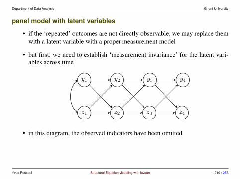
Department of Data Analysis Ghent University
panel model with latent variables
• if the ‘repeated’ outcomes are not directly observable, we may replace themwith a latent variable with a proper measurement model
• but first, we need to establish ‘measurement invariance’ for the latent vari-ables across time
y1 y2 y3 y4
z1 z2 z3 z4
• in this diagram, the observed indicators have been omitted
Yves Rosseel Structural Equation Modeling with lavaan 219 / 256
Department of Data Analysis Ghent University
strengths and limitations of panel models
• panel models can be very useful for examining the relations of two (or more)variables (observed or latent) over time
• often, we are equally interested in the lack of relations over time
• panel models do not tell us anything about group level tendencies (overallincrease or decrease of the scores)
• panel models do not tell us anything about individual tendencies
Yves Rosseel Structural Equation Modeling with lavaan 220 / 256
Department of Data Analysis Ghent University
real-world example
• example from the Curran & Bollen (2001) book chapter ‘The Best of TwoWorlds’
• topic: developmental relation between antisocial behavior and depressivesymptomatology
• original data come from the National Longitudinal Survey of Youth (NLSY);original 1979 panel included a total of 12,686 respondents
• in 1986, the children of the original NLSY female respondents were alsoincluded in the survey
• the sample used for this example only includes data of children that were8 years old at the first wave of measurement, have no missings on all fourwaves, only biological children, resulting in a final sample of N = 180
• we only include the sumscores of two constructs (antisocial behavior anddepressive symptomatology), measured at 4 time points
Yves Rosseel Structural Equation Modeling with lavaan 221 / 256

Department of Data Analysis Ghent University
preparing the sample statistics
• creating a covariance matrix for all 8 observed variables:
> lower <- '+ 2.926+ 1.390 4.257+ 1.698 2.781 4.536+ 1.628 2.437 2.979 5.605+ 1.240 0.789 0.903 1.278 3.208+ 0.592 1.890 1.419 1.004 1.706 3.994+ 0.929 1.278 1.900 1.000 1.567 1.654 3.583+ 0.659 0.949 1.731 2.420 0.988 1.170 1.146 3.649 '> COV <- getCov(lower, names=c("anti1", "anti2", "anti3", "anti4",+ "dep1", "dep2", "dep3", "dep4"))> MEANS <- c(1.750, 1.928, 1.978, 2.322, 2.178, 2.489, 2.294, 2.222)
questions
• what happens over time? how are the two constructs related to each other?
Yves Rosseel Structural Equation Modeling with lavaan 222 / 256

Department of Data Analysis Ghent University
test of equality of means over time: antisocial behavior
• model with 4 means, unequal variances, fully correlated
> model <- '+ # four repeated means+ anti1 ˜ i1*1; anti2 ˜ i2*1; anti3 ˜ i3*1; anti4 ˜ i4*1++ # four unequal variances+ anti1 ˜˜ anti1; anti2 ˜˜ anti2; anti3 ˜˜ anti3; anti4 ˜˜ anti4++ # fully correlated+ anti1 ˜˜ anti2 + anti3 + anti4+ anti2 ˜˜ anti3 + anti4+ anti3 ˜˜ anti4+ '> fit <- lavaan(model, sample.cov=COV, sample.mean=MEANS, sample.nobs=180,+ sample.cov.rescale=FALSE, mimic="EQS")> summary(fit)
lavaan 0.6-6.1508 ended normally after 40 iterations
Estimator MLOptimization method NLMINBNumber of free parameters 14
Number of observations 180
Yves Rosseel Structural Equation Modeling with lavaan 223 / 256
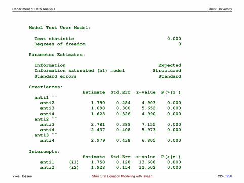
Department of Data Analysis Ghent University
Model Test User Model:
Test statistic 0.000Degrees of freedom 0
Parameter Estimates:
Information ExpectedInformation saturated (h1) model StructuredStandard errors Standard
Covariances:Estimate Std.Err z-value P(>|z|)
anti1 ˜˜anti2 1.390 0.284 4.903 0.000anti3 1.698 0.300 5.652 0.000anti4 1.628 0.326 4.990 0.000
anti2 ˜˜anti3 2.781 0.389 7.155 0.000anti4 2.437 0.408 5.973 0.000
anti3 ˜˜anti4 2.979 0.438 6.805 0.000
Intercepts:Estimate Std.Err z-value P(>|z|)
anti1 (i1) 1.750 0.128 13.688 0.000anti2 (i2) 1.928 0.154 12.502 0.000
Yves Rosseel Structural Equation Modeling with lavaan 224 / 256
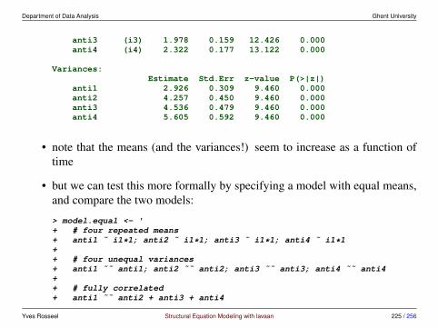
Department of Data Analysis Ghent University
anti3 (i3) 1.978 0.159 12.426 0.000anti4 (i4) 2.322 0.177 13.122 0.000
Variances:Estimate Std.Err z-value P(>|z|)
anti1 2.926 0.309 9.460 0.000anti2 4.257 0.450 9.460 0.000anti3 4.536 0.479 9.460 0.000anti4 5.605 0.592 9.460 0.000
• note that the means (and the variances!) seem to increase as a function oftime
• but we can test this more formally by specifying a model with equal means,and compare the two models:
> model.equal <- '+ # four repeated means+ anti1 ˜ i1*1; anti2 ˜ i1*1; anti3 ˜ i1*1; anti4 ˜ i1*1++ # four unequal variances+ anti1 ˜˜ anti1; anti2 ˜˜ anti2; anti3 ˜˜ anti3; anti4 ˜˜ anti4++ # fully correlated+ anti1 ˜˜ anti2 + anti3 + anti4
Yves Rosseel Structural Equation Modeling with lavaan 225 / 256
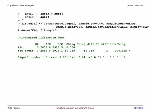
Department of Data Analysis Ghent University
+ anti2 ˜˜ anti3 + anti4+ anti3 ˜˜ anti4+ '> fit.equal <- lavaan(model.equal, sample.cov=COV, sample.mean=MEANS,+ sample.nobs=180, sample.cov.rescale=FALSE, mimic="EQS")> anova(fit, fit.equal)
Chi-Squared Difference Test
Df AIC BIC Chisq Chisq diff Df diff Pr(>Chisq)fit 0 2878.8 2923.5 0.000fit.equal 3 2884.0 2919.1 11.089 11.089 3 0.01125 *---Signif. codes: 0 '***' 0.001 '**' 0.01 '*' 0.05 '.' 0.1 ' ' 1
Yves Rosseel Structural Equation Modeling with lavaan 226 / 256

Department of Data Analysis Ghent University
first-order autoregressive model: antisocial behavior
• unequal autoregressive coefficients, unequal residual variances
> model <- '+ anti2 ˜ a21*anti1+ anti3 ˜ a32*anti2+ anti4 ˜ a43*anti3++ # one variance+ anti1 ˜˜ anti1++ # three (unqequal) residual variances+ anti2 ˜˜ anti2; anti3 ˜˜ anti3; anti4 ˜˜ anti4+ '> fit <- lavaan(model, sample.cov=COV, sample.mean=MEANS, sample.nobs=180,+ sample.cov.rescale=FALSE, mimic="EQS")> summary(fit)
lavaan 0.6-6.1508 ended normally after 23 iterations
Estimator MLOptimization method NLMINBNumber of free parameters 7
Number of observations 180
Yves Rosseel Structural Equation Modeling with lavaan 227 / 256
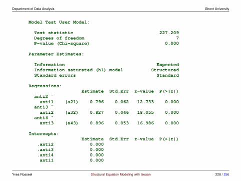
Department of Data Analysis Ghent University
Model Test User Model:
Test statistic 227.209Degrees of freedom 7P-value (Chi-square) 0.000
Parameter Estimates:
Information ExpectedInformation saturated (h1) model StructuredStandard errors Standard
Regressions:Estimate Std.Err z-value P(>|z|)
anti2 ˜anti1 (a21) 0.796 0.062 12.733 0.000
anti3 ˜anti2 (a32) 0.827 0.046 18.055 0.000
anti4 ˜anti3 (a43) 0.896 0.053 16.986 0.000
Intercepts:Estimate Std.Err z-value P(>|z|)
.anti2 0.000
.anti3 0.000
.anti4 0.000anti1 0.000
Yves Rosseel Structural Equation Modeling with lavaan 228 / 256

Department of Data Analysis Ghent University
Variances:Estimate Std.Err z-value P(>|z|)
anti1 5.988 0.633 9.460 0.000.anti2 4.184 0.442 9.460 0.000.anti3 2.995 0.317 9.460 0.000.anti4 4.210 0.445 9.460 0.000
• fit not very good; we could impose equality constraints (equal regressions,equal residuals), but the overall impression is that the autoregressive modeldoes not fit the data well
Yves Rosseel Structural Equation Modeling with lavaan 229 / 256
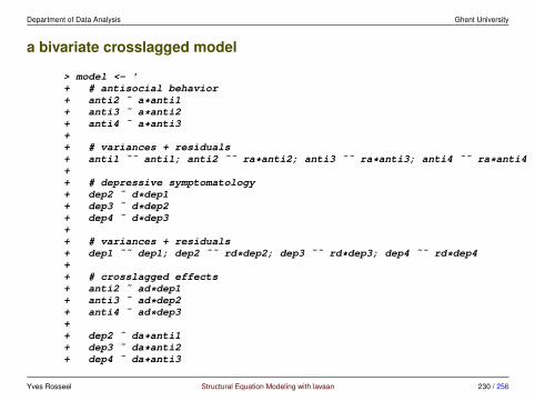
Department of Data Analysis Ghent University
a bivariate crosslagged model
> model <- '+ # antisocial behavior+ anti2 ˜ a*anti1+ anti3 ˜ a*anti2+ anti4 ˜ a*anti3++ # variances + residuals+ anti1 ˜˜ anti1; anti2 ˜˜ ra*anti2; anti3 ˜˜ ra*anti3; anti4 ˜˜ ra*anti4++ # depressive symptomatology+ dep2 ˜ d*dep1+ dep3 ˜ d*dep2+ dep4 ˜ d*dep3++ # variances + residuals+ dep1 ˜˜ dep1; dep2 ˜˜ rd*dep2; dep3 ˜˜ rd*dep3; dep4 ˜˜ rd*dep4++ # crosslagged effects+ anti2 ˜ ad*dep1+ anti3 ˜ ad*dep2+ anti4 ˜ ad*dep3++ dep2 ˜ da*anti1+ dep3 ˜ da*anti2+ dep4 ˜ da*anti3
Yves Rosseel Structural Equation Modeling with lavaan 230 / 256

Department of Data Analysis Ghent University
++ # correlated residuals within time+ anti1 ˜˜ dep1; anti2 ˜˜ c2*dep2; anti3 ˜˜ c2*dep3; anti4 ˜˜ c2*dep4+ '> fit <- lavaan(model, sample.cov=COV, sample.mean=MEANS, sample.nobs=180,+ sample.cov.rescale=FALSE, mimic="EQS")> summary(fit)
lavaan 0.6-6.1508 ended normally after 38 iterations
Estimator MLOptimization method NLMINBNumber of free parameters 24Number of equality constraints 14Row rank of the constraints matrix 14
Number of observations 180
Model Test User Model:
Test statistic 391.642Degrees of freedom 34P-value (Chi-square) 0.000
Parameter Estimates:
Information ExpectedInformation saturated (h1) model Structured
Yves Rosseel Structural Equation Modeling with lavaan 231 / 256

Department of Data Analysis Ghent University
Standard errors Standard
Regressions:Estimate Std.Err z-value P(>|z|)
anti2 ˜anti1 (a) 0.692 0.044 15.843 0.000
anti3 ˜anti2 (a) 0.692 0.044 15.843 0.000
anti4 ˜anti3 (a) 0.692 0.044 15.843 0.000
dep2 ˜dep1 (d) 0.582 0.042 13.899 0.000
dep3 ˜dep2 (d) 0.582 0.042 13.899 0.000
dep4 ˜dep3 (d) 0.582 0.042 13.899 0.000
anti2 ˜dep1 (ad) 0.188 0.042 4.473 0.000
anti3 ˜dep2 (ad) 0.188 0.042 4.473 0.000
anti4 ˜dep3 (ad) 0.188 0.042 4.473 0.000
dep2 ˜anti1 (da) 0.276 0.044 6.346 0.000
dep3 ˜anti2 (da) 0.276 0.044 6.346 0.000
dep4 ˜anti3 (da) 0.276 0.044 6.346 0.000
Yves Rosseel Structural Equation Modeling with lavaan 232 / 256
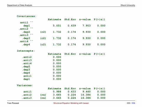
Department of Data Analysis Ghent University
Covariances:Estimate Std.Err z-value P(>|z|)
anti1 ˜˜dep1 5.051 0.639 7.903 0.000
.anti2 ˜˜.dep2 (c2) 1.732 0.174 9.930 0.000
.anti3 ˜˜.dep3 (c2) 1.732 0.174 9.930 0.000
.anti4 ˜˜.dep4 (c2) 1.732 0.174 9.930 0.000
Intercepts:Estimate Std.Err z-value P(>|z|)
.anti2 0.000
.anti3 0.000
.anti4 0.000
.dep2 0.000
.dep3 0.000
.dep4 0.000anti1 0.000dep1 0.000
Variances:Estimate Std.Err z-value P(>|z|)
anti1 5.988 0.633 9.460 0.000.anti2 (ra) 3.665 0.224 16.386 0.000.anti3 (ra) 3.665 0.224 16.386 0.000
Yves Rosseel Structural Equation Modeling with lavaan 233 / 256

Department of Data Analysis Ghent University
.anti4 (ra) 3.665 0.224 16.386 0.000dep1 7.952 0.841 9.460 0.000
.dep2 (rd) 3.638 0.222 16.386 0.000
.dep3 (rd) 3.638 0.222 16.386 0.000
.dep4 (rd) 3.638 0.222 16.386 0.000
• it would seem that earlier antisocial behavior predicts later depressive symp-tomatology, but not vice versa
• however, we should be careful with these parameters because the model doesnot fit the data well!
Yves Rosseel Structural Equation Modeling with lavaan 234 / 256
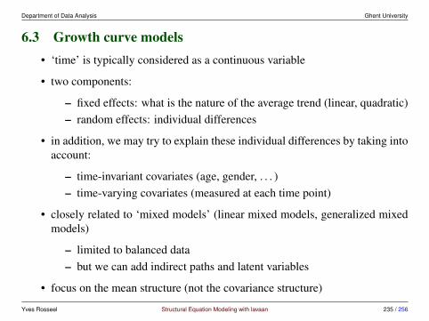
Department of Data Analysis Ghent University
6.3 Growth curve models• ‘time’ is typically considered as a continuous variable
• two components:
– fixed effects: what is the nature of the average trend (linear, quadratic)– random effects: individual differences
• in addition, we may try to explain these individual differences by taking intoaccount:
– time-invariant covariates (age, gender, . . . )– time-varying covariates (measured at each time point)
• closely related to ‘mixed models’ (linear mixed models, generalized mixedmodels)
– limited to balanced data– but we can add indirect paths and latent variables
• focus on the mean structure (not the covariance structure)
Yves Rosseel Structural Equation Modeling with lavaan 235 / 256
Department of Data Analysis Ghent University
some references
• Bollen, K.A., & Curran, P.J. (2006). Latent curve models: A structuralequation perspective. John Wiley & Sons.
• Duncan, T.E., Duncan, S.C., & Strycker, L.A. (2006). An introduction tolatent variable growth curve modeling: Concepts, issues, and applications.Routledge Academic.
• Preacher, K.J., Wichman, A.L., MacCallum, R.C., & Briggs, N.E. (2008).Latent Growth Curve Modeling. Quantitative Applications in the Social Sci-ences, No. 157, Sage.
Yves Rosseel Structural Equation Modeling with lavaan 236 / 256

Department of Data Analysis Ghent University
random intercept
• creating a random intercept:
y1 y2 y3 y4 y5
ε1 ε2 ε3 ε4 ε5
intercept
1 1 1 1 1
Yves Rosseel Structural Equation Modeling with lavaan 237 / 256

Department of Data Analysis Ghent University
random intercept only, positive linear trend
• a random-intercept-only model assumes that all individuals follow the sametrend, but with a different initial point (intercept)
Yves Rosseel Structural Equation Modeling with lavaan 238 / 256

Department of Data Analysis Ghent University
R code
• when using the sem() or cfa() fitting functions, you need to manually setthe intercepts of the observed repeated variables to zero, and free the latentintercept:
> model <- '+ # random intercept+ int =˜ 1*y1 + 1*y2 + 1*y3 + 1*y4 + 1*y5++ # zero intercepts+ y1 + y2 + y3 + y4 + y5 ˜ 0*1++ # free latent intercept+ int ˜ 1+ '
• the growth() fitting function does this automatically (for all latent variables):
> model <- '+ # random intercept+ int =˜ 1*y1 + 1*y2 + 1*y3 + 1*y4 + 1*y5+ '
Yves Rosseel Structural Equation Modeling with lavaan 239 / 256
Department of Data Analysis Ghent University
• when both ‘regular’ latent variables, and ‘random effects’ are used in thesame model, it is perhaps better to use the lavaan() function:
> model <- '+ # random intercept+ int =˜ 1*y1 + 1*y2 + 1*y3 + 1*y4 + 1*y5++ # free latent intercept and variance+ int ˜ 1+ int ˜˜ int++ # add residual variances+ y1 ˜˜ y1; y2 ˜˜ y2; y3 ˜˜ y3; y4 ˜˜ y4; y5 ˜˜ y5+ '
Yves Rosseel Structural Equation Modeling with lavaan 240 / 256

Department of Data Analysis Ghent University
random slope
• creating a random slope:
y1 y2 y3 y4 y5
ε1 ε2 ε3 ε4 ε5
slope
0 1 2 3 4
• here, the ‘reference’ point is the first time point; another coding scheme (-4,-3, -2, -1, 0) treats the last time point as the reference point
• this will not affect model fit, but it will change the interpretation of the pa-rameters
Yves Rosseel Structural Equation Modeling with lavaan 241 / 256
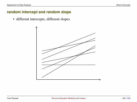
Department of Data Analysis Ghent University
random intercept and random slope
• different intercepts, different slopes
Yves Rosseel Structural Equation Modeling with lavaan 242 / 256
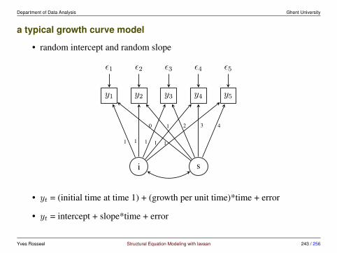
Department of Data Analysis Ghent University
a typical growth curve model
• random intercept and random slope
y1 y2 y3 y4 y5
ε1 ε2 ε3 ε4 ε5
i s
1 1 1 1 1
0 1 2 3 4
• yt = (initial time at time 1) + (growth per unit time)*time + error
• yt = intercept + slope*time + error
Yves Rosseel Structural Equation Modeling with lavaan 243 / 256
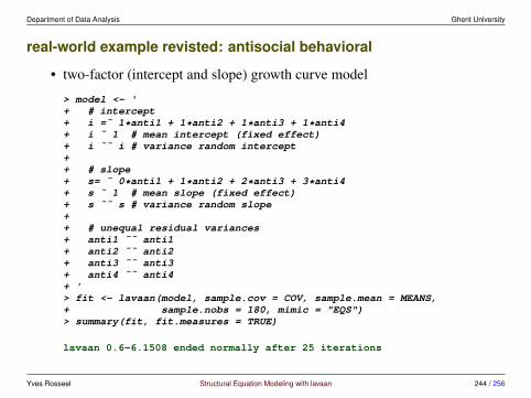
Department of Data Analysis Ghent University
real-world example revisted: antisocial behavioral
• two-factor (intercept and slope) growth curve model
> model <- '+ # intercept+ i =˜ 1*anti1 + 1*anti2 + 1*anti3 + 1*anti4+ i ˜ 1 # mean intercept (fixed effect)+ i ˜˜ i # variance random intercept++ # slope+ s= ˜ 0*anti1 + 1*anti2 + 2*anti3 + 3*anti4+ s ˜ 1 # mean slope (fixed effect)+ s ˜˜ s # variance random slope++ # unequal residual variances+ anti1 ˜˜ anti1+ anti2 ˜˜ anti2+ anti3 ˜˜ anti3+ anti4 ˜˜ anti4+ '> fit <- lavaan(model, sample.cov = COV, sample.mean = MEANS,+ sample.nobs = 180, mimic = "EQS")> summary(fit, fit.measures = TRUE)
lavaan 0.6-6.1508 ended normally after 25 iterations
Yves Rosseel Structural Equation Modeling with lavaan 244 / 256

Department of Data Analysis Ghent University
Estimator MLOptimization method NLMINBNumber of free parameters 8
Number of observations 180
Model Test User Model:
Test statistic 14.810Degrees of freedom 6P-value (Chi-square) 0.022
Model Test Baseline Model:
Test statistic 227.618Degrees of freedom 6P-value 0.000
User Model versus Baseline Model:
Comparative Fit Index (CFI) 0.960Tucker-Lewis Index (TLI) 0.960
Loglikelihood and Information Criteria:
Loglikelihood user model (H0) -1432.849Loglikelihood unrestricted model (H1) -1425.402
Yves Rosseel Structural Equation Modeling with lavaan 245 / 256
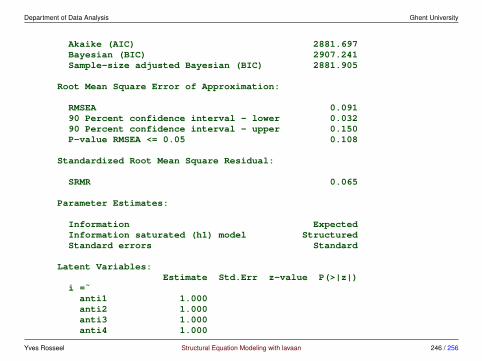
Department of Data Analysis Ghent University
Akaike (AIC) 2881.697Bayesian (BIC) 2907.241Sample-size adjusted Bayesian (BIC) 2881.905
Root Mean Square Error of Approximation:
RMSEA 0.09190 Percent confidence interval - lower 0.03290 Percent confidence interval - upper 0.150P-value RMSEA <= 0.05 0.108
Standardized Root Mean Square Residual:
SRMR 0.065
Parameter Estimates:
Information ExpectedInformation saturated (h1) model StructuredStandard errors Standard
Latent Variables:Estimate Std.Err z-value P(>|z|)
i =˜anti1 1.000anti2 1.000anti3 1.000anti4 1.000
Yves Rosseel Structural Equation Modeling with lavaan 246 / 256
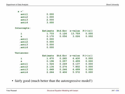
Department of Data Analysis Ghent University
s =˜anti1 0.000anti2 1.000anti3 2.000anti4 3.000
Intercepts:Estimate Std.Err z-value P(>|z|)
i 1.733 0.126 13.759 0.000s 0.170 0.056 3.026 0.002
.anti1 0.000
.anti2 0.000
.anti3 0.000
.anti4 0.000
Variances:Estimate Std.Err z-value P(>|z|)
i 1.670 0.260 6.430 0.000s 0.198 0.057 3.499 0.000
.anti1 1.526 0.249 6.137 0.000
.anti2 2.136 0.274 7.802 0.000
.anti3 1.648 0.246 6.699 0.000
.anti4 2.264 0.406 5.572 0.000
• fairly good (much better than the autoregressive model!)
Yves Rosseel Structural Equation Modeling with lavaan 247 / 256

Department of Data Analysis Ghent University
6.4 Alternative models• autoregressive latent trajectory (ALT) models
• latent change score models
• . . .
Yves Rosseel Structural Equation Modeling with lavaan 248 / 256

Department of Data Analysis Ghent University
autoregressive latent trajectory (ALT) models
• Bollen & Curran, in a series of papers (1999, 2000, 2001, 2004) proposed ahybrid model they called the ‘autoregressive latent trajectory’ (ALT) model;best reference:
Bollen, K.A., & Curran, P.J. (2004). Autoregressive latent trajec-tory (ALT) models: a synthesis of two traditions. SociologicalMethods & Research, 32(3), 336-383.
• it is a growth curve model, combined with an autoregressive structure for therepeated measures
• can be used when there is interest in both continuous underlying trajectoriesand time-specific influences across constructs
• the authors described this approach as ‘The Best of Both Worlds’
• nevertheless, the approach has been criticized because the interpretation isnot always clear; perhaps we should have the autoregressive structure at thelevel of the residuals errors?
Yves Rosseel Structural Equation Modeling with lavaan 249 / 256
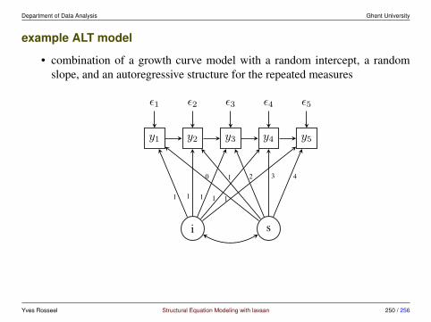
Department of Data Analysis Ghent University
example ALT model
• combination of a growth curve model with a random intercept, a randomslope, and an autoregressive structure for the repeated measures
y1 y2 y3 y4 y5
ε1 ε2 ε3 ε4 ε5
i s
1 1 1 1 1
0 1 2 3 4
Yves Rosseel Structural Equation Modeling with lavaan 250 / 256
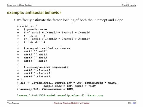
Department of Data Analysis Ghent University
example: antisocial behavior
• we freely estimate the factor loading of both the intercept and slope> model <- '+ # growth curve+ i =˜ anti1 + 1*anti2 + 1*anti3 + 1*anti4+ i ˜ 1; i ˜˜ i+ s= ˜ anti1 + 1*anti2 + 2*anti3 + 3*anti4+ s ˜ 1; s ˜˜ s++ # unequal residual variances+ anti1 ˜˜ anti1+ anti2 ˜˜ anti2+ anti3 ˜˜ anti3+ anti4 ˜˜ anti4++ # autoregressive components+ anti2 ˜ a1*anti1+ anti3 ˜ a2*anti2+ anti4 ˜ a3*anti3+ '> fit <- lavaan(model, sample.cov = COV, sample.mean = MEANS,+ sample.nobs = 180, mimic = "EQS")> summary(fit, fit.measures = TRUE)
lavaan 0.6-6.1508 ended normally after 61 iterations
Yves Rosseel Structural Equation Modeling with lavaan 251 / 256
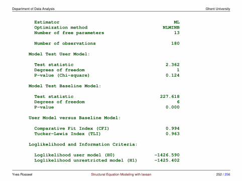
Department of Data Analysis Ghent University
Estimator MLOptimization method NLMINBNumber of free parameters 13
Number of observations 180
Model Test User Model:
Test statistic 2.362Degrees of freedom 1P-value (Chi-square) 0.124
Model Test Baseline Model:
Test statistic 227.618Degrees of freedom 6P-value 0.000
User Model versus Baseline Model:
Comparative Fit Index (CFI) 0.994Tucker-Lewis Index (TLI) 0.963
Loglikelihood and Information Criteria:
Loglikelihood user model (H0) -1426.590Loglikelihood unrestricted model (H1) -1425.402
Yves Rosseel Structural Equation Modeling with lavaan 252 / 256

Department of Data Analysis Ghent University
Akaike (AIC) 2879.179Bayesian (BIC) 2920.688Sample-size adjusted Bayesian (BIC) 2879.517
Root Mean Square Error of Approximation:
RMSEA 0.08790 Percent confidence interval - lower 0.00090 Percent confidence interval - upper 0.238P-value RMSEA <= 0.05 0.206
Standardized Root Mean Square Residual:
SRMR 0.026
Parameter Estimates:
Information ExpectedInformation saturated (h1) model StructuredStandard errors Standard
Latent Variables:Estimate Std.Err z-value P(>|z|)
i =˜anti1 0.967 0.116 8.311 0.000anti2 1.000anti3 1.000anti4 1.000
Yves Rosseel Structural Equation Modeling with lavaan 253 / 256

Department of Data Analysis Ghent University
s =˜anti1 1.050 0.475 2.210 0.027anti2 1.000anti3 2.000anti4 3.000
Regressions:Estimate Std.Err z-value P(>|z|)
anti2 ˜anti1 (a1) 0.020 0.160 0.127 0.899
anti3 ˜anti2 (a2) 0.351 0.148 2.375 0.018
anti4 ˜anti3 (a3) 0.677 0.221 3.066 0.002
Intercepts:Estimate Std.Err z-value P(>|z|)
i 2.321 0.392 5.917 0.000s -0.471 0.184 -2.566 0.010
.anti1 0.000
.anti2 0.000
.anti3 0.000
.anti4 0.000
Variances:Estimate Std.Err z-value P(>|z|)
i 1.825 0.700 2.609 0.009s -0.350 0.133 -2.635 0.008
Yves Rosseel Structural Equation Modeling with lavaan 254 / 256

Department of Data Analysis Ghent University
.anti1 1.596 0.334 4.775 0.000
.anti2 2.795 0.470 5.943 0.000
.anti3 2.545 0.511 4.982 0.000
.anti4 5.108 1.323 3.861 0.000
• note the negative variance for the slope factor!
Yves Rosseel Structural Equation Modeling with lavaan 255 / 256

Department of Data Analysis Ghent University
Thank you for attending this workshop!
Yves Rosseel Structural Equation Modeling with lavaan 256 / 256

![Basic lavaan Syntax Guide - Amazon Web Services · 1. Getting Started [top] A few basic points: Lavaan is an R package for classical structural equation modeling (SEM). An elementary](https://img.pdfslide.us/doc/110x75/5f178debd681f80b571b5cbe/basic-lavaan-syntax-guide-amazon-web-services-1-getting-started-top-a-few-basic.jpg)


![Estimating and interpreting structural equation models … · Estimating and interpreting structural equation models in Stata 12 ... and Var [ǫ] = Σ sem (y1 ... Structural equation](https://img.pdfslide.us/doc/110x75/5b286e167f8b9ae8108b4592/estimating-and-interpreting-structural-equation-models-estimating-and-interpreting.jpg)