Embed Size (px)
Citation preview
R. R. BurridgeTexas Robotics and Automation CenterMetrica, Inc.Houston, Texas 77058, [email protected]
A. A. RizziThe Robotics InstituteCarnegie Mellon UniversityPittsburgh, Pennsylvania 15213-3891, [email protected]
D. E. KoditschekArtificial Intelligence Laboratory and Controls LaboratoryDepartment of Electrical Engineering and Computer ScienceUniversity of MichiganAnn Arbor, Michigan 48109-2110, [email protected]
SequentialCompositionof DynamicallyDexterous RobotBehaviors
Abstract
We report on our efforts to develop a sequential robot controller-composition technique in the context of dexterous “batting” maneu-vers. A robot with a flat paddle is required to strike repeatedly ata thrown ball until the ball is brought to rest on the paddle at aspecified location. The robot’s reachable workspace is blocked byan obstacle that disconnects the free space formed when the ball andpaddle remain in contact, forcing the machine to “let go” for a timeto bring the ball to the desired state. The controller compositionswe create guarantee that a ball introduced in the “safe workspace”remains there and is ultimately brought to the goal. We report onexperimental results from an implementation of these formal compo-sition methods, and present descriptive statistics characterizing theexperiments.
KEY WORDS—hybrid control, controller composition, dy-namical dexterity, switching control, reactive scheduling,backchaining, obstacle avoidance
1. Introduction
We are interested in tasks requiring dynamical dexterity—the ability to perform work on the environment by effectingchanges in its kinetic as well as potential energy. Specifically,
The International Journal of Robotics ResearchVol. 18, No. 6, June 1999, pp. 534-555,©1999 Sage Publications, Inc.
we want to explore the control issues that arise from dynamicalinteractions between robot and environment, such as activebalancing, hopping, throwing, catching, and juggling. At thesame time, we wish to explore how such dexterous behaviorscan be marshaled toward goals whose achievement requiresat least the rudiments of strategy.
In this paper, we explore empirically a simple but for-mal approach to the sequential composition of robot behav-iors. We cast “behaviors” —robotic implementations of user-specified tasks—in a form amenable to representation as stateregulation via feedback to a specified goal set in the pres-ence of obstacles. Our approach results ideally in a partitionof state space induced by a palette of pre-existing feedbackcontrollers. Each cell of this partition is associated with aunique controller, chosen in such a fashion that entry into anycell guarantees passage to successively “lower” cells until the“lowest,” the goal cell, has been achieved. The domain ofattraction to the goal set for the resulting switching controlleris shown to be formed from the union of the domains of theconstituent controllers.1
1.1. Statement of the Problem
We have chosen the task domain of paddle juggling as one thatepitomizes dynamically dexterous behavior. The ball will fallto the floor unless repeatedly struck from below or balancedon the paddle surface. Thus the dynamics of the environment
1. Portions of this paper have appeared in an earlier work (Burridge 1996).
534
Burridge, Rizzi, and Koditschek / Dynamically Dexterous Robot Behaviors 535
necessitate continual action from the robot. Moreover, theintermittent nature of the robot-ball interaction provides a fo-cused test bed for studying the hybrid (mixed continuous anddiscrete) control problems that arise in many areas of robotics.In this paper, the machine must acquire and contain a thrownball, maneuver it through the workspace while avoiding ob-stacles that necessitate regrasping2 along the way, and finallybring it to rest on the paddle at a desired location. We referto this task asdynamical pick and place(DPP). By explicitlyintroducing obstacles,3 and requiring a formal guarantee thatthe system will not drive the ball into them, we add a strategicelement to the task.
From the perspective of control theory, our notion of “be-havior” comprises merely the closed-loop dynamics of a plantoperating under feedback. Yet for our task, as is often thecase when trying to control a dynamical system, no avail-able feedback control algorithm will successfully stabilize aslarge a range of initial conditions as desired. Instead, thereexists a collection of control laws, each capable of stabiliz-ing a different local region of the system’s state space. Ifthey were properly coordinated, the region of the workspaceacross which their combined influence might be exerted wouldbe significantly larger than the domain of attraction for anyone of the available local controllers. The process of creatinga switching strategy between control modes is an aspect ofhybrid control theory that is not presently well established.In this paper, we use conservative approximations of the do-mains of attraction and goal sets of the local controllers tocreate a “prepares” graph. Then, backchaining away fromthe controller that stabilizes the task goal, we use the graphto create a partition of the state space of the robot into re-gions within each of which a unique controller is active. Thisleads to the creation of complex switching controllers withformal stability properties, and this specific instance of sta-ble hybrid control represents our present notion of behavioralcomposition.
To test our methods, we use a three-degree-of-freedomrobot whose paddle-juggling capabilities are already well es-tablished (Rizzi 1994). Although our available juggling con-trol laws induce very good regulation about their respectivegoal sets, there will always be ball states that each cannotcontain: the goal sets have limited domains of attraction.However, many of the states that are “uncontainable” by onecontrol law can be successfully handled by another with dif-ferent parameter settings, such as a new goal point, or per-
2. In general, regrasping is required when the free configuration space at-tendant upon the current grasp is disconnected, and the goal does not lie inthe presently occupied connected component. As will be seen, in the DPPproblem the configuration space of the “palming” grasp disconnects the goalfrom the component in which the ball is typically introduced. The robot canonly “connect” the two components by adopting a “juggling” grasp, whoseconfiguration space has a dramatically different topology.3. The finite length of the paddle has always induced an implicit obstacle,but we have not hitherto modeled or accounted for it in our juggling work(Rizzi, Whitcomb, and Koditschek 1992).
haps different gain settings. In this paper, we resort solely tosuch parameter retunings to explore the problem of behavioralcomposition. For all aspects of the robot’s task—containingthe initial throw, moving the ball through the workspace, ne-gotiating the obstacle that divides the workspace, and finallybringing the ball to rest on the paddle—we require that it usemembers of an established palette of juggling control lawswith different goal points or gain tunings.
Our group has explored paddle juggling for some time(Rizzi, Whitcomb, and Koditschek 1992; Rizzi 1994), andit should be emphasized here that this is not a paper aboutjuggling per se. Rather, our juggling apparatus provides aconvenient test bed for the more general switching controlmethods presented in Section 3, which necessitate the explo-ration of the juggling behavior described in Section 2.5.
1.2. Previous Literature
1.2.1. Pick and Place in Cluttered Environments
Our focus on the dynamical pick-and-place problem is in-spired in part by the Handey system developed by Lozano-Pérez and colleagues (Lozano-Pérez, et al. 1987), who em-phasized the importance of developing task-planning capabil-ities suitable for situations where regrasping is necessitatedby environmental clutter (see footnote 1); however, our setuppresents dynamical rather than quasi-static regrasping prob-lems. Indeed, our emphasis on robustness and error recoveryas the driving considerations in robot task planning derivesfrom their original insights on fine-motion planning (Lozano-Pérez, Mason, and Taylor 1984), and the subsequent literaturein this tradition bears a close relation to our concerns, as istouched upon below.
Comprehensive work by Tung and Kak (1994) yielded acontemporary quasi-static assembly environment in the besttraditions of the Handey apparatus. The system built a planbased on sensed initial conditions, spawned an execution pro-cess that sensed exceptions to the planned evolution of states,and produced actions to bring the world’s state back to theintermediate situation presumed by the plan. We wish to ex-amine the ways in which this higher level “feedback” (localreplanningis a form of feedback) can be reasoned about andguaranteed to succeed, albeit in the drastically simplified set-ting of the dynamical pick-and-place problem outlined above.
1.2.2. Hybrid Control and Discrete-Event Systems
The difficult question of how to reason about the interplay be-tween sensing and recovery at the event level in robotics hasbeen considerably stimulated by the advent of the Ramadge-Wonham DES control paradigm (Ramadge and Wonham1987). In some of the most careful and convincing ofsuch DES-inspired robotics papers, Lyons proposed a for-malism for encoding and reasoning about the construction ofaction plans and their sensor-based execution (Lyons 1993;
536 THE INTERNATIONAL JOURNAL OF ROBOTICS RESEARCH / June 1999
Lyons and Hendriks 1994). In contrast to our interest, how-ever, Lyons explicitly avoided the consideration of problemswherein geometric and force-sensor reports must be used toestimate progress, and thereby stimulate the appropriate eventtransitions.
1.2.3. Error Detection and Recovery
Despite the many dissimilarities in problem domain, models,and representation, the work discussed here seems to bear theclosest correspondence to the “fine-motion planning with un-certainty” literature in robotics (for example, as discussed inLatombe’s text (Latombe 1991)) originated by Lozano-Pérez,Mason, and Taylor (1984). Traditionally, this literature fo-cuses on quasi-static problems (generalized damper dynam-ics (Whitney 1977) with Coulomb reaction forces (Erdmann1984) on the contact set). Furthermore, the possible controlactions typically are restricted to piecewise constant-velocityvectors, whereby each constant piece is corrupted by a con-stant disturbance vector of bounded magnitude and unknowndirection. In contrast, we are interested in Newtonian dy-namical models, and our control primitive is not a constantaction, but rather the entire range of actions consequent on theclosed-loop policy,8, to be specified below. Differences inmodels notwithstanding, we have derived considerable mo-tivation from the “LMT” (Lozano-Pérez, Mason, and Taylor1984) framework as detailed in Section 1.3.3.
1.2.4. Juggling
In an earlier work (Burridge, Rizzi, and Koditschek 1997),we introduced the notions of dynamical safety and obsta-cle avoidance, and in 1995 we discussed the controller-composition algorithm mentioned in Section 3 (Burridge,Rizzi, and Koditschek 1995). The major contribution of thispaper is in furthering our work by showing how to composecontrollers in such a manner as to avoid an obstacle that dis-connects the workspace.
In previous work in our lab (Buehler, Koditschek, andKindlmann 1990b; Rizzi and Koditschek 1994), a great dealof attention has been paid to the lower level palette of con-trollers. Our architecture implements event-driven robot poli-cies whose resulting closed-loop dynamics drive the coupledrobot-environment state toward a goal set. We strive to de-velop control algorithms that are sufficiently tractable as toallow correctness guarantees with estimates of the domain ofattraction as well. Thus, we have focused theoretical attentionon “practicable stability mechanisms”—dynamical systemsfor which effectively computable local tests provide global(or, at least, over a “large” volume) conclusions. At the sametime, we have focused experimental attention on building adistributed computational environment that supports flexiblyreconfigurable combinations of sensor and actuator hardwarecontrollers, motion estimation and control algorithms, and
event-driven reference-trajectory generators. The result hasbeen a series of laboratory robots that exhibit indefatigablegoal-seeking behavior, albeit in a very narrow range of tasks.In this paper, we explore the “higher level” problem of gen-eralizing the range of tasks by composing the existing con-trollers, achieving new tasks that no single existing controlleris capable of in isolation.
1.3. Overview of the Approach
1.3.1. Feedback Confers Robustness
Physical disturbances to a system can be classified, broadlyspeaking, into two categories. The first includes the small,persistent disturbances arising from model inaccuracies andsensor and actuator noise. Ball spin, air drag on a ball mod-eled as a point mass, and spurious changes in camera measure-ments introduced by lighting variations in a scene representtypical examples of this first type of disturbance. The secondcategory includes large, significant changes to the world asexpected. For example, if a parts tray is severely jostled or ar-rives unexpectedly empty, an assembly robot’s world modelis likely to have been grossly violated. Such large distur-bances occur very rarely (otherwise, they would have beenaccounted for systematically by the robot’s designers!), butare potentially catastrophic.
A common tradition in robotics and control has been tomodel these disturbances in the hope of treating them ratio-nally. One typically appeals to stochastic representations ofsmall perturbations, and introduces an optimal design (for ex-ample, a Kalman filter) to handle them. Analogously, recov-ery from catastrophe is similarly model-based, typically beingaddressed by special “exception-handling” routines specifi-cally written for each particular failure anticipated. But dis-turbances are generally left out of nominal models preciselybecause they are so difficult to model. The systematic originof the typical small disturbance often defies a stochastic rep-resentation, and the resulting optimal designs may be overlyaggressive. If the human system designers haven’t imagineda severe failure mode, then the system will be unable to reactto it when it occurs, with possibly disastrous results.
Feedback-controlled systems can be designed to confer alevel of robustness against both types of disturbance with-out recourse to explicit disturbance models. On one hand,asymptotically stable systems are generically locally struc-turally stable. This means that the first class of disturbancescan degrade performance (e.g., biasing the goal set, or coars-ening the neighborhood of the goal set to which all initialconditions in its domain of attraction are eventually brought),but if small enough, they cannot destroy the stability of the(possibly biased) goal. On the other hand, if the closed-loopsystem induced by a feedback controller exhibits a global (orat least “large”) domain of attraction, then large disturbancescan never “take it by surprise,” as long as the original state
Burridge, Rizzi, and Koditschek / Dynamically Dexterous Robot Behaviors 537
space and dynamical model used to represent the world (notthe disturbance) remain valid following the perturbation. Thesystem will merely continue to pursue the same shepherdingfunction, now applied at the new state, with the same tire-less progression toward the goal as before. Of course, suchdisturbances need to be rare relative to the time required torecover from them, or we should not expect the system to everapproach the goal.
1.3.2. Feedback Strategies as Funnels
A decade ago, Mason introduced the notion of a funnel asa metaphor for the robust, self-organizing emergent behav-ior displayed by otherwise unactuated masses in the presenceof passive mechanical guideways (Mason 1985).4 He under-stood that the shape of the guideways constituted an embodiedcomputational mechanism of control that ought to be renderedprogrammable. In this paper, we embrace Mason’s metaphorand seek to extend it to active electromechanical systems (i.e.,possessing sensors and actuators) which are more obviouslyprogrammable.
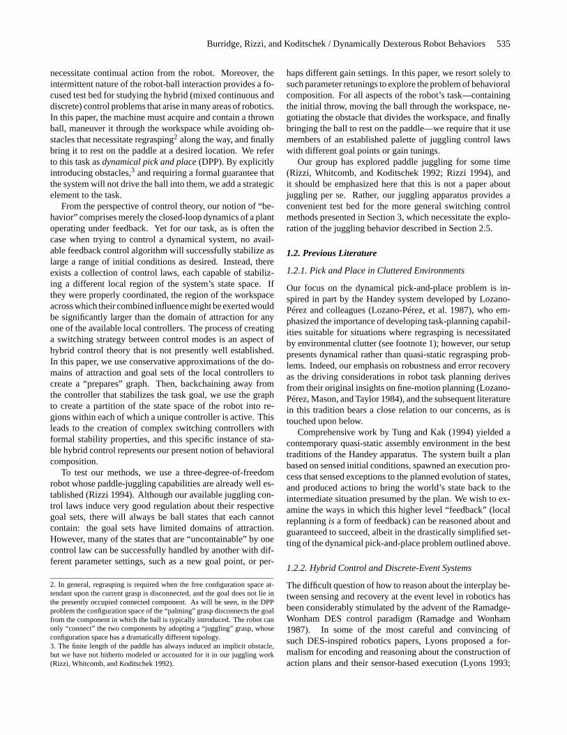
Figure 1 depicts the idealized graph of a positive-definitescalar-valued function centered at a goal point—its only zeroand unique minimum. If a feedback control strategy resultsin closed-loop dynamics on the domain (depicted as thex−yplane in these figures) such that all motions, when projectedup onto the funnel, lead strictly downward (z < 0), thenthis funnel is said to be a Lyapunov function. In such a case,Mason’s metaphor of sand falling down a funnel is particularlyrelevant, since all initial conditions on the plane lying beneaththe over-spreading shoulders of the funnel (now interpretedas the graph of the Lyapunov function) will be drawn downthe funnel toward its center—the goal.
Although the funnels strictly represent Lyapunov func-tions, which may be difficult to find, we note that such func-tions must exist within the domain of attraction for all asymp-totically stable dynamical systems. Thus we loosen our no-tion of “funnels,” and let them represent attracting dynamicalsystems, with the extent of the funnel representing a knowninvariant region (for a Lyapunov function, this would be anyof the level curves).
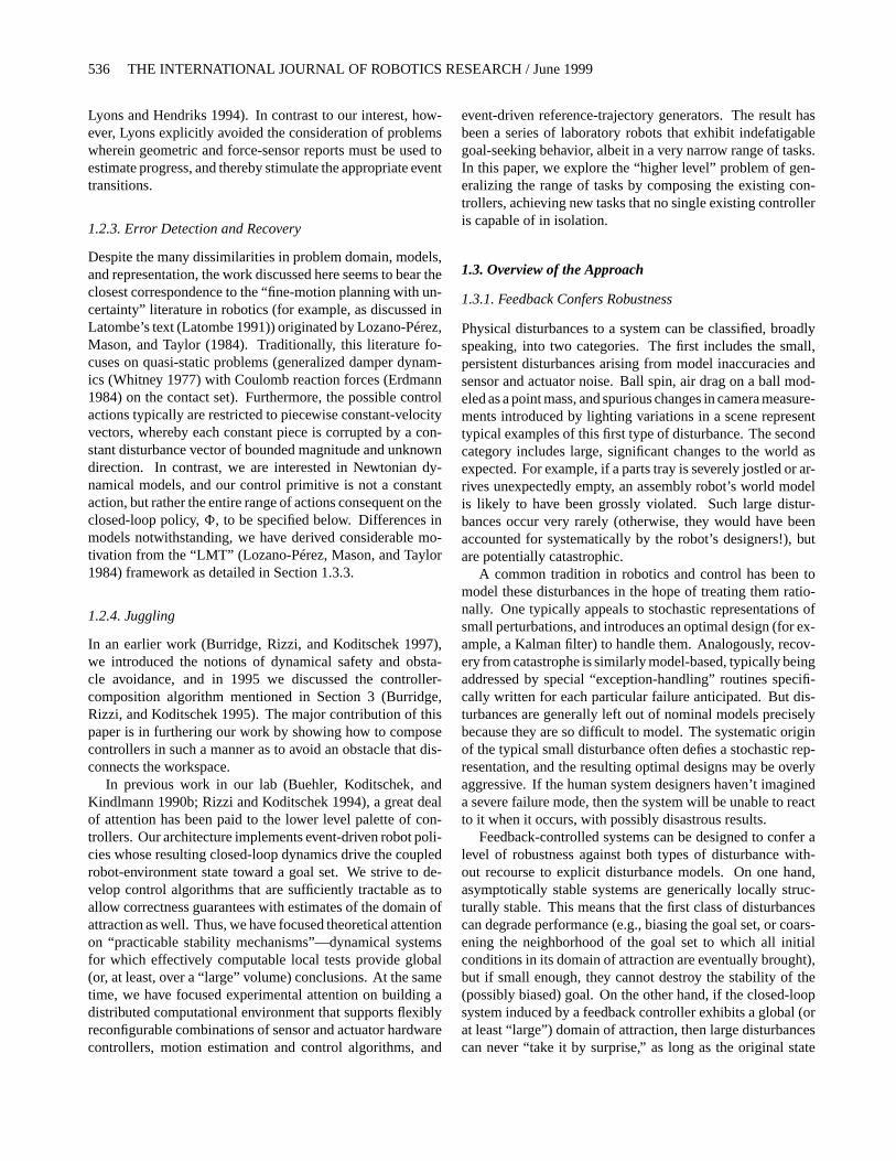
In Figure 2, we depict a complicated boundary such asmight arise when the user specifies an “obstacle”—here, allstates outside the bounded area of “good” states.5 Ideally,we would like a control strategy that funnels all “good” statesto the goal, without allowing any to enter the obstacle. Wesuggest this in the figure by sketching a complex funnel whoseshape is exactly adapted to the domain.6 Unfortunately, it is
4. Other researchers in robotics and fine-motion planning have introducedcomparable metaphors (Ish-Shalom 1984; Lozano-Pérez, Mason, and Taylor1984).5. Of course, this picture dramatically understates the potential complexity ofsuch problems, since the free space need not be simply connected as depicted.6. Rimon and Koditschek (1992) addressed the design of such global fun-nels for purely geometric problems, wherein the complicated portion of the
Fig. 1. The Lyapunov function as a funnel: an idealizedgraph of a positive-definite function over its state space.
usually very difficult or impossible to find globally attractivecontrol laws, so Figure 2 often cannot be realized, for practicalreasons. Moreover, there is a large and important class ofmechanical systems for which no single funnel (continuous-stabilizing feedback law) exists (Brockett 1983; Koditschek1992). Nevertheless, one need not yet abandon the recourseto feedback.
1.3.3. Sequential Composition as Preimage Backchaining
We turn next to a tradition from the fine-motion planningliterature, introduced by Lozano-Pérez, Mason, and Taylor(1984)—the notion of preimage backchaining. Suppose wehave a palette of controllers whose induced funnels have goalsets that can be placed at will throughout the obstacle-freestate space. Then we may deploy a collection of controllerswhose combined (local) domains of attraction cover a largepart of the relevant region of the state space (e.g., states withinsome bound of the origin). If such a set is rich enough that thedomains overlap and each controller’s goal set lies within thedomains of other controllers, then it is possible tobackchainaway from the overall task goal, partitioning the state spaceinto cells in which the different controllers will be active, andarrive at a scheme for switching between the controllers thatwill provably drive any state in the union of all the variousdomains to the single task-goal state.
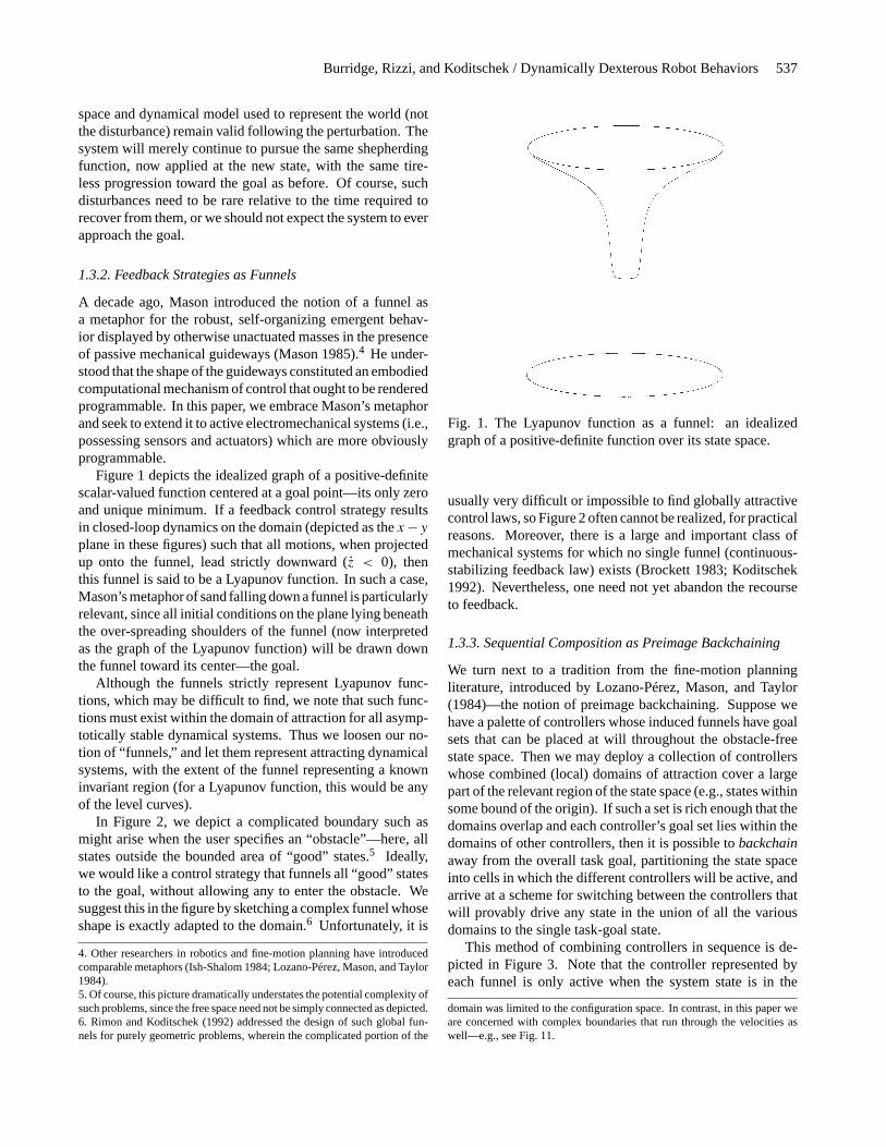
This method of combining controllers in sequence is de-picted in Figure 3. Note that the controller represented byeach funnel is only active when the system state is in the
domain was limited to the configuration space. In contrast, in this paper weare concerned with complex boundaries that run through the velocities aswell—e.g., see Fig. 11.
538 THE INTERNATIONAL JOURNAL OF ROBOTICS RESEARCH / June 1999
Fig. 2. An ideal funnel capturing the entire obstacle-free statespace of the system.
appropriate region of the state space (beyond the reach oflower funnels), as sketched at the bottom of the figure, andindicated by the dashed portion of the funnel. As each con-troller drives the system toward its local goal, the state crossesa boundary into another region of state space where anothercontroller is active. This process is repeated until the statereaches the final cell, which is the only one to contain thegoal set of its own controller.
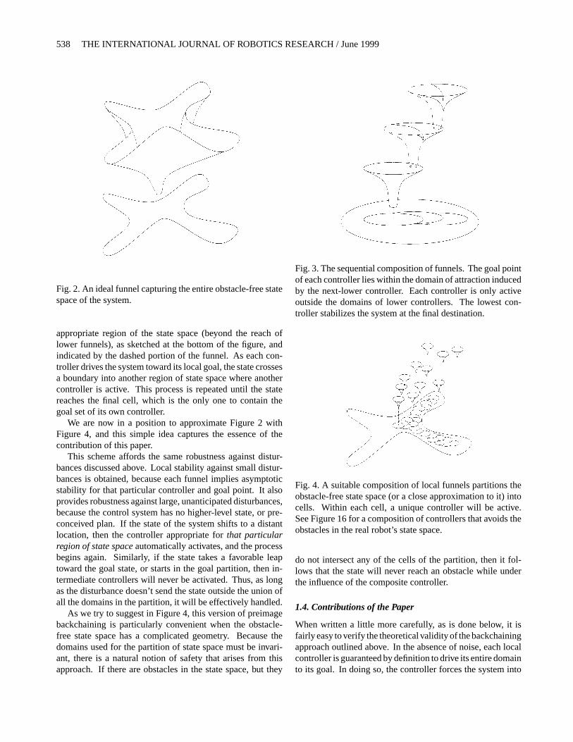
We are now in a position to approximate Figure 2 withFigure 4, and this simple idea captures the essence of thecontribution of this paper.
This scheme affords the same robustness against distur-bances discussed above. Local stability against small distur-bances is obtained, because each funnel implies asymptoticstability for that particular controller and goal point. It alsoprovides robustness against large, unanticipated disturbances,because the control system has no higher-level state, or pre-conceived plan. If the state of the system shifts to a distantlocation, then the controller appropriate forthat particularregion of state spaceautomatically activates, and the processbegins again. Similarly, if the state takes a favorable leaptoward the goal state, or starts in the goal partition, then in-termediate controllers will never be activated. Thus, as longas the disturbance doesn’t send the state outside the union ofall the domains in the partition, it will be effectively handled.
As we try to suggest in Figure 4, this version of preimagebackchaining is particularly convenient when the obstacle-free state space has a complicated geometry. Because thedomains used for the partition of state space must be invari-ant, there is a natural notion of safety that arises from thisapproach. If there are obstacles in the state space, but they
Fig. 3. The sequential composition of funnels. The goal pointof each controller lies within the domain of attraction inducedby the next-lower controller. Each controller is only activeoutside the domains of lower controllers. The lowest con-troller stabilizes the system at the final destination.
Fig. 4. A suitable composition of local funnels partitions theobstacle-free state space (or a close approximation to it) intocells. Within each cell, a unique controller will be active.See Figure 16 for a composition of controllers that avoids theobstacles in the real robot’s state space.
do not intersect any of the cells of the partition, then it fol-lows that the state will never reach an obstacle while underthe influence of the composite controller.
1.4. Contributions of the Paper
When written a little more carefully, as is done below, it isfairly easy to verify the theoretical validity of the backchainingapproach outlined above. In the absence of noise, each localcontroller is guaranteed by definition to drive its entire domainto its goal. In doing so, the controller forces the system into
Burridge, Rizzi, and Koditschek / Dynamically Dexterous Robot Behaviors 539
the domain of a higher-priority controller. This process mustrepeat until the domain of the goal controller is reached.
For the nonlinear problems that inevitably arise in robotics,however, invariant domains of attraction are difficult to de-rive in closed form, so the utility of the approach is calledinto question. Moreover, physical systems are inevitably“messier” than the abstracted models their designers intro-duce for convenience, and the question arises whether theseideas incur an overly optimistic reliance on closed-loop mod-els. Modeling errors may, for instance, destroy the correctnessof our method, allowing cycling among the controllers. Thuswe must turn to empirical tests to verify that our formallycorrect method can produce useful controllers in practice.
The experimental environment for our juggling robot ishighly nonlinear and “messy,” and challenges the idealizedview of the formal method in several ways. We have noclosed-form Lyapunov functions from which to choose ourdomains of attraction. Instead, we are forced to use conser-vative invariant regions found using experimental data andnumerical simulation. Also, there is significant local noisein the steady-state behavior of the system, so that even our“invariant” regions are occasionally violated. Nevertheless,as will be shown, our composition method proves to be veryrobust in the face of these problems. We are able to create apalette of controllers that successfully handles a wide range ofinitial conditions, persevering to the task goal while avoidingthe obstacles, despite the significant noise along the way.
1.5. Organization of the Paper
This paper follows a logical development roughly suggestedby Figures 1–4. In Section 2, we provide a high-level overviewof the hardware and software, describe how entries in thecontroller palette (suggested by Fig. 1) arise, and introducetheJuggle, 8J , a controller used as a basis for all entries inour palette. We also introduce variants of8J : catching,8C ;and palming,8P . In Section 3, we introduce the notion ofa safe controller suggested by Figure 2, as well as formallydefine the sequential composition depicted in Figure 3. InSection 4, we implement the partition suggested by Figure 4,and report on our empirical results.
2. The Physical Setting
2.1. The Hardware System
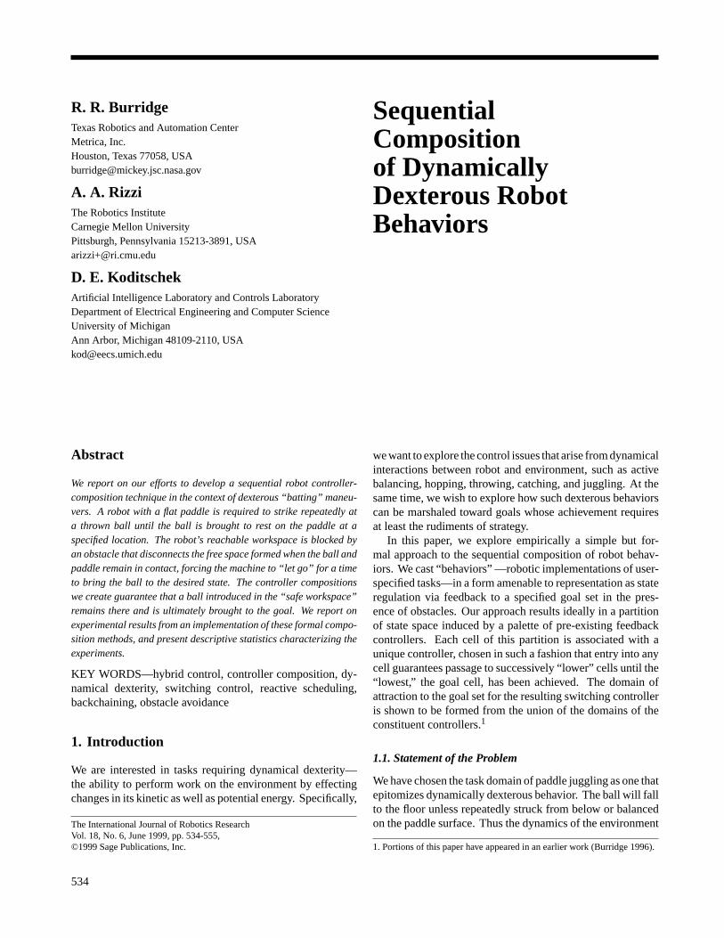
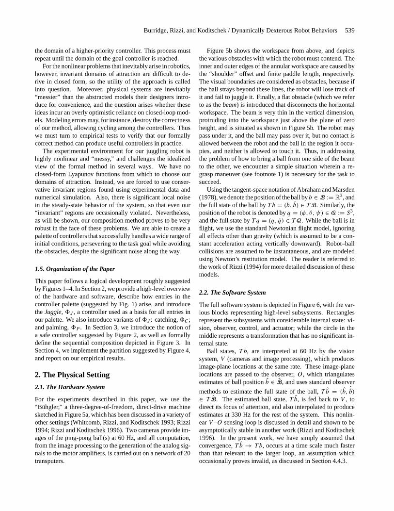
For the experiments described in this paper, we use the“Bühgler,” a three-degree-of-freedom, direct-drive machinesketched in Figure 5a, which has been discussed in a variety ofother settings (Whitcomb, Rizzi, and Koditschek 1993; Rizzi1994; Rizzi and Koditschek 1996). Two cameras provide im-ages of the ping-pong ball(s) at 60 Hz, and all computation,from the image processing to the generation of the analog sig-nals to the motor amplifiers, is carried out on a network of 20transputers.
Figure 5b shows the workspace from above, and depictsthe various obstacles with which the robot must contend. Theinner and outer edges of the annular workspace are caused bythe “shoulder” offset and finite paddle length, respectively.The visual boundaries are considered as obstacles, because ifthe ball strays beyond these lines, the robot will lose track ofit and fail to juggle it. Finally, a flat obstacle (which we referto as thebeam) is introduced that disconnects the horizontalworkspace. The beam is very thin in the vertical dimension,protruding into the workspace just above the plane of zeroheight, and is situated as shown in Figure 5b. The robot maypass under it, and the ball may pass over it, but no contact isallowed between the robot and the ball in the region it occu-pies, and neither is allowed to touch it. Thus, in addressingthe problem of how to bring a ball from one side of the beamto the other, we encounter a simple situation wherein a re-grasp maneuver (see footnote 1) is necessary for the task tosucceed.
Using the tangent-space notation of Abraham and Marsden(1978), we denote the position of the ball byb ∈ B := R
3, andthe full state of the ball byT b = (b, b) ∈ TB. Similarly, theposition of the robot is denoted byq = (φ, θ, ψ) ∈ Q := S3,and the full state byT q = (q, q) ∈ TQ. While the ball is inflight, we use the standard Newtonian flight model, ignoringall effects other than gravity (which is assumed to be a con-stant acceleration acting vertically downward). Robot–ballcollisions are assumed to be instantaneous, and are modeledusing Newton’s restitution model. The reader is referred tothe work of Rizzi (1994) for more detailed discussion of thesemodels.
2.2. The Software System
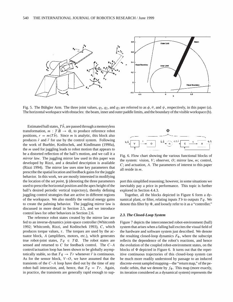
The full software system is depicted in Figure 6, with the var-ious blocks representing high-level subsystems. Rectanglesrepresent the subsystems with considerable internal state: vi-sion, observer, control, and actuator; while the circle in themiddle represents a transformation that has no significant in-ternal state.
Ball states,T b, are interpreted at 60 Hz by the visionsystem,V (cameras and image processing), which producesimage-plane locations at the same rate. These image-planelocations are passed to the observer,O, which triangulatesestimates of ball positionb ∈ B, and uses standard observer
methods to estimate the full state of the ball,T b = (b, ˆb)∈ T B. The estimated ball state,T b, is fed back toV , todirect its focus of attention, and also interpolated to produceestimates at 330 Hz for the rest of the system. This nonlin-earV –O sensing loop is discussed in detail and shown to beasymptotically stable in another work (Rizzi and Koditschek1996). In the present work, we have simply assumed thatconvergence,T b → T b, occurs at a time scale much fasterthan that relevant to the larger loop, an assumption whichoccasionally proves invalid, as discussed in Section 4.4.3.
540 THE INTERNATIONAL JOURNAL OF ROBOTICS RESEARCH / June 1999
Fig. 5. The Bühgler Arm. The three joint values,q1, q2, andq3 are referred to asφ, θ , andψ , respectively, in this paper (a).The horizontal workspace with obstacles: the beam, inner and outer paddle limits, and the boundary of the visible workspace (b).
Estimated ball states,T b, are passed through a memorylesstransformation,m : T B → Q, to produce reference robotpositions,r = m(T b). Sincem is analytic, this block alsoproducesr and r for use by the control system. Followingthe work of Buehler, Koditschek, and Kindlmann (1990a),them used for juggling leads to robot motion that appears tobe a distorted reflection of the ball’s motion, and we call it amirror law. The juggling mirror law used in this paper wasdeveloped by Rizzi, and a detailed description is available(Rizzi 1994). The mirror law uses nine key parameters thatprescribe the spatial location and feedback gains for the jugglebehavior. In this work, we are mostly interested in modifyingthe location of theset point, G (denoting the three parametersused to prescribe horizontal position and the apex height of theball’s desired periodic vertical trajectory), thereby definingjuggling control strategies that are active in different regionsof the workspace. We also modify the vertical energy gainsto create the palming behavior. The juggling mirror law isdiscussed in more detail in Section 2.5, and we introducecontrol laws for other behaviors in Section 2.6.
The reference robot states created by the mirror law arefed to an inverse-dynamics joint-space controller (Whitcomb1992; Whitcomb, Rizzi, and Koditschek 1993),C, whichproduces torque values,τ . The torques are used by the ac-tuator block,A (amplifiers, motors, etc.), which generatestrue robot-joint states,T q ∈ TQ. The robot states aresensed and returned toC for feedback control. TheC–Acontrol/actuation loop has been shown to be globally asymp-totically stable, so thatT q → T r wheneverr is continuous.As for the sensor block,V –O, we have assumed that thetransients of theC–A loop have died out by the time of anyrobot–ball interaction, and, hence, thatT q = T r. Again,in practice, the transients are generally rapid enough to sup-
Fig. 6. Flow chart showing the various functional blocks ofthe system: vision,V ; observer,O; mirror law,m; control,C; and actuation,A. The parameters of interest to this paperall reside inm.
port this simplified reasoning; however, in some situations weinevitably pay a price in performance. This topic is furtherexplored in Section 4.4.3.
Together, all the blocks depicted in Figure 6 form a dy-namical plant, or filter, relating inputsT b to outputsT q. Wedenote this filter by8, and loosely refer to it as a “controller.”
2.3. The Closed-Loop System
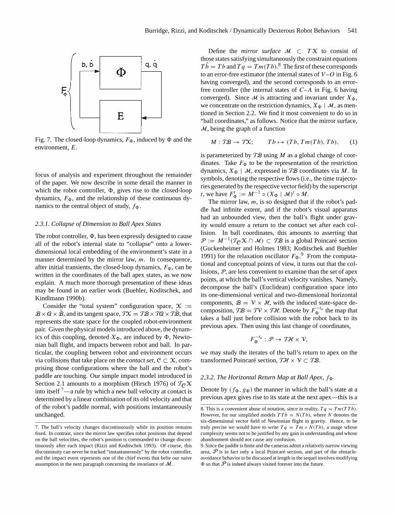
Figure 7 depicts the interconnected robot-environment (ball)system that arises when a falling ball excites the visual field ofthe hardware and software system just described. We denotethe resulting closed-loop dynamicsF8, where the subscriptreflects the dependence of the robot’s reactions, and hencethe evolution of the coupled robot-environment states, on theblocks of8 depicted in Figure 6. It turns out that the repet-itive continuous trajectories of this closed-loop system canbe much more readily understood by passage to an induceddiscrete-event sampled mapping—the “return map,” of the pe-riodic orbits, that we denote byf8. This map (more exactly,its iteration considered as a dynamical system) represents the
Burridge, Rizzi, and Koditschek / Dynamically Dexterous Robot Behaviors 541
Fig. 7. The closed-loop dynamics,F8, induced by8 and theenvironment,E.
focus of analysis and experiment throughout the remainderof the paper. We now describe in some detail the manner inwhich the robot controller,8, gives rise to the closed-loopdynamics,F8, and the relationship of these continuous dy-namics to the central object of study,f8.
2.3.1. Collapse of Dimension to Ball Apex States
The robot controller,8, has been expressly designed to causeall of the robot’s internal state to “collapse” onto a lower-dimensional local embedding of the environment’s state in amanner determined by the mirror law,m. In consequence,after initial transients, the closed-loop dynamics,F8, can bewritten in the coordinates of the ball apex states, as we nowexplain. A much more thorough presentation of these ideasmay be found in an earlier work (Buehler, Koditschek, andKindlmann 1990b).
Consider the “total system” configuration space,X :=B×Q×B, and its tangent space,TX = TB×TQ×TB, thatrepresents the state space for the coupled robot-environmentpair. Given the physical models introduced above, the dynam-ics of this coupling, denotedX8, are induced by8, Newto-nian ball flight, and impacts between robot and ball. In par-ticular, the coupling between robot and environment occursvia collisions that take place on thecontact set,C ⊂ X, com-prising those configurations where the ball and the robot’spaddle are touching. Our simple impact model introduced inSection 2.1 amounts to a morphism (Hirsch 1976) ofTCXinto itself 7—a rule by which a new ball velocity at contact isdetermined by a linear combination of its old velocity and thatof the robot’s paddle normal, with positions instantaneouslyunchanged.
7. The ball’s velocity changes discontinuously while its position remainsfixed. In contrast, since the mirror law specifies robot positions that dependon the ball velocities, the robot’s position is commanded to change discon-tinuously after each impact (Rizzi and Koditschek 1993). Of course, thisdiscontinuity can never be tracked “instantaneously” by the robot controller,and the impact event represents one of the chief events that belie our naiveassumption in the next paragraph concerning the invariance ofM.
Define the mirror surface M ⊂ TX to consist ofthose states satisfying simultaneously the constraint equationsT b = T b andT q = Tm(T b).8 The first of these correspondsto an error-free estimator (the internal states ofV –O in Fig. 6having converged), and the second corresponds to an error-free controller (the internal states ofC–A in Fig. 6 havingconverged). SinceM is attracting and invariant underX8,we concentrate on the restriction dynamics,X8 | M, as men-tioned in Section 2.2. We find it most convenient to do so in“ball coordinates,” as follows. Notice that the mirror surface,M, being the graph of a function
M : TB → TX; T b 7→ (T b, T m(T b), T b), (1)
is parameterized byTB usingM as a global change of coor-dinates. TakeF8 to be the representation of the restrictiondynamics,X8 | M, expressed inTB coordinates viaM. Insymbols, denoting the respective flows (i.e., the time trajecto-ries generated by the respective vector field) by the superscriptt , we haveF t8 := M−1 ◦ (X8 | M)t ◦M.
The mirror law,m, is so designed that if the robot’s pad-dle had infinite extent, and if the robot’s visual apparatushad an unbounded view, then the ball’s flight under grav-ity would ensure a return to the contact set after each col-lision. In ball coordinates, this amounts to asserting thatP := M−1(TCX ∩ M) ⊂ TB is a global Poincaré section(Guckenheimer and Holmes 1983; Koditschek and Buehler1991) for the relaxation oscillatorF8.9 From the computa-tional and conceptual points of view, it turns out that the col-lisions,P, are less convenient to examine than the set of apexpoints, at which the ball’s vertical velocity vanishes. Namely,decompose the ball’s (Euclidean) configuration space intoits one-dimensional vertical and two-dimensional horizontalcomponents,B = V × H, with the induced state-space de-composition,TB = TV × TH. Denote byF−ta
8 the map thattakes a ball just before collision with the robot back to itsprevious apex. Then using this last change of coordinates,
F−ta8 : P → TH × V,
we may study the iterates of the ball’s return to apex on thetransformed Poincaré section,TH × V ⊂ TB.
2.3.2. The Horizontal Return Map at Ball Apex,f8
Denote by(f8, g8) the manner in which the ball’s state at aprevious apex gives rise to its state at the next apex—this is a
8. This is a convenient abuse of notation, since in reality,T q = Tm(T T b).
However, for our simplified modelsT T b = N(T b), whereN denotes thesix-dimensional vector field of Newtonian flight in gravity. Hence, to betruly precise we would have to writeT q = Tm ◦ N(T b), a usage whosecomplexity seems not to be justified by any gain in understanding and whoseabandonment should not cause any confusion.9. Since the paddle is finite and the cameras admit a relatively narrow viewingarea,P is in fact only a local Poincaré section, and part of the obstacle-avoidance behavior to be discussed at length in the sequel involves modifying8 so thatP is indeed always visited forever into the future.
542 THE INTERNATIONAL JOURNAL OF ROBOTICS RESEARCH / June 1999
mapping fromTH × V onto itself. Buehler, Koditschek, andKindlmann (1990a, 1990b) showed that when the jugglingmirror law is restricted toV, g8 has global attraction toGV(the vertical component of the set point). In contrast, onlylocal attraction of(f8, g8) toGH×GV has been demonstratedto date.
Furthermore, Rizzi and Koditschek (1994) showed thatf8andg8 are nearly decoupled. Indeed, empirical results con-firm that the horizontal behavior off8 changes very littlewithin a large range of apex heights, and that the vertical sys-tem is regulated much faster than the horizontal.
Thus, except where otherwise specified, we ignoreVthroughout this paper, and concentrate our attention on theevolution of f8 in TH. Accordingly, for ease of exposi-tion, we denote the horizontal goal setG (dropping theHsubscript), a singleton subset ofTH comprising a desiredhorizontal position at zero velocity.
2.4. Obstacles
In this section, we briefly describe the origin of the obstaclesin TH × V with which we are concerned. We must start byreverting back to the full six-dimensional space,TB, and therestriction flowF t8. Although we attempt to be fairly thoroughin this section, some details are omitted in the interest ofreadability. The reader is referred to two other works (Rizzi1994; Burridge 1996) for the missing details.
There are three types of physical obstacle with which weare concerned. The first consists of regions of the robot spacethat are “off limits” to the robot,OQ ⊂ Q, whether or notit is in contact with the ball. Robot obstacles include thefloor, joint limits, etc., as well as any physical obstacle inthe workspace, and have been studied in the kinematics lit-erature. Recall that for a particular mirror law,m, each ballstate induces a corresponding robot state. Stretching our ter-minology, we loosely definem−1(OQ) = {T b ∈ TB|m(T b)∈ OQ}.
The second type of physical obstacle consists of subsets ofball state space which are off limits to the ball,OTB ⊂ TB,whether or not it is touching the robot. This set may includewalls, the floor, visual boundaries, and any other objects inthe workspace that the ball should avoid (such as the beam).Note that this region resides in the full state space of the ball,so for example, if the vision system fails for ball velocitiesabove a certain value at certain locations, such states can beincluded inOTB.
The final type of physical obstacle is defined as the set ofball states that are “lost.” Intuitively, this set, which we callthe workspace obstacle, OWS, consists of all ball states onthe boundary of the workspace that are never coming back.
We combine these three types into one general physicalobstacle,
O = m−1(OQ)⋃
OTB⋃
OWS,
occupying the ball’s configuration space.
These physical obstacles must be “dilated” in the (discrete-time) domain off8 to account for physical collisions thatmay occur during the continuous-time interval between apexevents. We proceed as follows.
For any ball state,T b , denote byτO+(T b) the time to
reach the physical obstacle,
τO+(T b) = min t > 0 : F t(T b) ∈ TO,
and by τO−(T b) the time elapsed from the last physical
obstacle,
τO−(T b) = max t < 0 : F t(T b) ∈ TO.
Similarly, denote the times to contact with the robot by
τ8+(T b) = min t > 0 : M ◦ F t(T b) ∈ TC,
and
τ8−(T b) = min t < 0 : ∃T x ∈ TC : F t ◦ Imp(T x) = T b,
whereImp is the impact map.A discrete obstacle is any apex state whose future
continuous-time trajectory must intersect the obstacle, orwhose past continuous-time trajectory may have intersectedthe obstacle,
O := {T b ∈ TH × V : τ+O(T b)
< τ+9 (T b)
∨τ−O(T b) > τ−
φ (T b)}.We will return to obstacles in the discussion on Safety, inSection 3.2.
2.5. Example: The Juggle8J
The generic juggling behavior developed by Rizzi for the Büh-gler is induced by a family of control laws in which a singleball is struck repeatedly by the robot paddle in such a wayas to direct it toward a limit cycle characterized by a singlezero-velocity apex point, orset point, G ⊂ H (we ignorethe vertical component here). We refer to members of thisgeneric class of controllers as8J . Under the assumptionsmade in Section 2.3,8J reduces to its associated mirror law,mJ , which is detailed elsewhere (Rizzi and Koditschek 1993;Rizzi 1994) and described below.
2.5.1. The Mirror Law,mJ
For a given ball state,T b, we begin by inverting the kinematicsof the arm to calculate a robot position that would just touchthe ball:q(b) = (φb, θb,0) (recall eq. (5)). We chooseψ = 0to eliminate redundancy. This effectively gives us the ball injoint-space coordinates.
Next, we express informally a robot strategy that causesthe paddle to respond to the motions of the ball in four ways.Here,φr , θr , andψr refer to the commanded joint values,whereasφb andθb refer to the values necessary for the paddleto touch the ball:
Burridge, Rizzi, and Koditschek / Dynamically Dexterous Robot Behaviors 543
1. φr = φb causes the paddle to track under the ball at alltimes.
2. θr mirrors the vertical motion of the ball (as it evolves inθb): as the ball goes up, the paddle goes down, and vice-versa, meeting at zero height. Differences between thedesired and actual total ball energy lead to changes inpaddle velocity at impact.
3. Radial motion or offset of the ball causes changes inθr ,resulting in a slight adjustment of the normal at impact,tending to push the ball back toward the set point.
4. Angular motion or offset of the ball causes changes inψr , again adjusting the normal so as to correct for lateralposition errors.
For the exact formulation ofmJ , the reader is referred toRizzi’s earlier work (Rizzi 1994).
The mirror law has three parameters for each of the threecylindrical coordinates (angular, radial, and vertical): a setpoint, and two PD gains. In Section 2.6, we will set thevertical gains to zero to create qualitatively different behavior(palming), while in Section 4 we will generate a family ofdifferent juggling controllers by changing only the angularset point.
2.5.2. Analysis, Simulation, and Empirical Exploration of theDomain of Attraction,D(8J )
The mirror law used in the experiments discussed in this paperdoes not permit a closed-form expression for the apex-apexreturn map. Recently we have made strides toward develop-ing a mirror law that has a solvable return map (Rizzi andKoditschek 1994), yet still generates similar behavior. As isseen in the sequel, this would be very helpful to our methods,but the absence of closed-form expressions does not impedethe ideas introduced in Section 1.3.
We define thedomain of attractionof 8 to G by D(8) ={T b ∈ TB : lim
n→∞fn8(T b) = G} in the absence of obstacles.
For the choice of mirror-law parameters used in this paper,D(8) contains nearly all ofTB such that the ball is abovethe paddle. In Section 3.2, we will constrain this definitionby incorporating all the obstacles from Section 2.4.
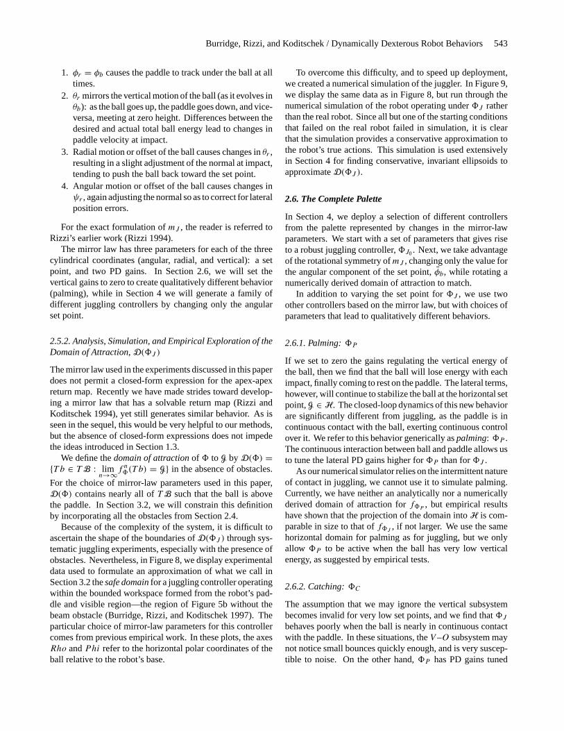
Because of the complexity of the system, it is difficult toascertain the shape of the boundaries ofD(8J ) through sys-tematic juggling experiments, especially with the presence ofobstacles. Nevertheless, in Figure 8, we display experimentaldata used to formulate an approximation of what we call inSection 3.2 thesafe domainfor a juggling controller operatingwithin the bounded workspace formed from the robot’s pad-dle and visible region—the region of Figure 5b without thebeam obstacle (Burridge, Rizzi, and Koditschek 1997). Theparticular choice of mirror-law parameters for this controllercomes from previous empirical work. In these plots, the axesRho andPhi refer to the horizontal polar coordinates of theball relative to the robot’s base.
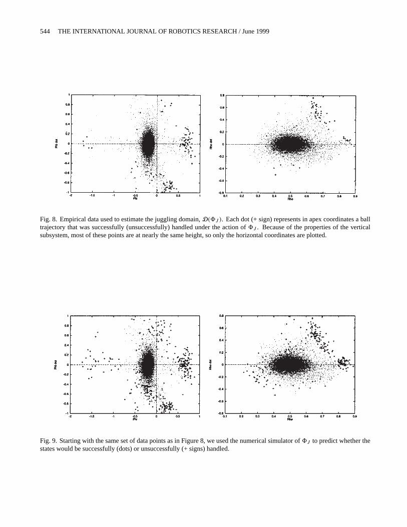
To overcome this difficulty, and to speed up deployment,we created a numerical simulation of the juggler. In Figure 9,we display the same data as in Figure 8, but run through thenumerical simulation of the robot operating under8J ratherthan the real robot. Since all but one of the starting conditionsthat failed on the real robot failed in simulation, it is clearthat the simulation provides a conservative approximation tothe robot’s true actions. This simulation is used extensivelyin Section 4 for finding conservative, invariant ellipsoids toapproximateD(8J ).
2.6. The Complete Palette
In Section 4, we deploy a selection of different controllersfrom the palette represented by changes in the mirror-lawparameters. We start with a set of parameters that gives riseto a robust juggling controller,8J0. Next, we take advantageof the rotational symmetry ofmJ , changing only the value forthe angular component of the set point,φb, while rotating anumerically derived domain of attraction to match.
In addition to varying the set point for8J , we use twoother controllers based on the mirror law, but with choices ofparameters that lead to qualitatively different behaviors.
2.6.1. Palming:8P
If we set to zero the gains regulating the vertical energy ofthe ball, then we find that the ball will lose energy with eachimpact, finally coming to rest on the paddle. The lateral terms,however, will continue to stabilize the ball at the horizontal setpoint,G ∈ H. The closed-loop dynamics of this new behaviorare significantly different from juggling, as the paddle is incontinuous contact with the ball, exerting continuous controlover it. We refer to this behavior generically aspalming: 8P .The continuous interaction between ball and paddle allows usto tune the lateral PD gains higher for8P than for8J .
As our numerical simulator relies on the intermittent natureof contact in juggling, we cannot use it to simulate palming.Currently, we have neither an analytically nor a numericallyderived domain of attraction forf8P , but empirical resultshave shown that the projection of the domain intoH is com-parable in size to that off8J , if not larger. We use the samehorizontal domain for palming as for juggling, but we onlyallow 8P to be active when the ball has very low verticalenergy, as suggested by empirical tests.
2.6.2. Catching:8C
The assumption that we may ignore the vertical subsystembecomes invalid for very low set points, and we find that8Jbehaves poorly when the ball is nearly in continuous contactwith the paddle. In these situations, theV –O subsystem maynot notice small bounces quickly enough, and is very suscep-tible to noise. On the other hand,8P has PD gains tuned
544 THE INTERNATIONAL JOURNAL OF ROBOTICS RESEARCH / June 1999
Fig. 8. Empirical data used to estimate the juggling domain,D(8J ). Each dot (+ sign) represents in apex coordinates a balltrajectory that was successfully (unsuccessfully) handled under the action of8J . Because of the properties of the verticalsubsystem, most of these points are at nearly the same height, so only the horizontal coordinates are plotted.
Fig. 9. Starting with the same set of data points as in Figure 8, we used the numerical simulator of8J to predict whether thestates would be successfully (dots) or unsuccessfully (+ signs) handled.
Burridge, Rizzi, and Koditschek / Dynamically Dexterous Robot Behaviors 545
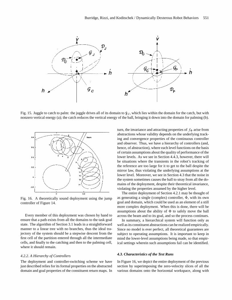
too aggressively for such bounces of the ball, and should beswitched on only when the ball is essentially resting on thepaddle. To guarantee a smooth transition from juggling topalming, we introduce acatchingcontroller,8C , designed todrain the vertical energy from the ball and bring it down closeto rest on the paddle. Currently, a variant of8J is used inwhich the vertical set point is very low, and the robot meetsthe ball higher than normal for8J . For an intuitive view ofhow the domains for8J ,8C , and8P overlap, see Figure 15.
Owing to the mixed nature of this controller, we have nei-ther analytical nor numerical approximations to its domain ofattraction. Instead, we use a very conservative estimate basedon the numerically derivedD(8J0) of Section 4.1. Althoughthis controller is not ideal, it removes enough of the verticalenergy from the ball that we can safely turn on palming. Cur-rently, catching is the dominant source of task failures, as wereport in Section 4.4.
3. The Formal Idea: Safe SequentialComposition
The technique proposed here is a variant of the preimagebackchaining idea introduced by Lozano-Pérez, Mason, andTaylor (1984), although their algorithm was used for compli-ant motion in quasi-static environments. We substitute sen-sory events for the physical transitions that characterized theircontrol sequences.
3.1. Sequential Composition
Say that controller81 preparescontroller82 (denoted81 �82) if the goal of the first lies within the domain of thesecond: G(81) ⊂ D(82). For any set of controllers,U = {81, ..., 8N }, this relation induces a directed (gener-ally cyclic) graph, denoted0.
Assume that the overall task goal,G, coincides with thegoal of at least one controller, which we call81: G(81) =G.10 Starting at the node of0 corresponding to81, we tra-verse the graph breadth-first, keeping only those arcs thatpoint back in the direction of81, thus ending up with anacyclic subgraph,0′ ⊂ 0. The construction of0′ induces apartial ordering ofU, but the algorithm below actually inducesa total ordering, with one controller being handled during eachiteration of the loop.
In the following algorithm, we recursively process con-trollers inU in a breadth-first manner leading away from81.We buildU′(N) ⊂ U, the set of all controllers that have beenprocessed so far, and its domain,DN(U
′), which is the unionof the domains of its elements. As we process each controller,8i , we define a subset of its domain,C(8i) ⊂ D(8i), that is
10. If the goal set of more than one controller coincides withG, then wechoose one arbitrarily (e.g., the one with the largest domain), and note thatall of the others will be added to the queue in the first iteration of the algorithm.
the cell of the partition of state space within which8i shouldbe active.
1. Let the queue contain81. Let C(81) = D(81), N =1, U′(1) = {81}, andD1(U
′) = D(81).
2. Remove the first element of the queue, and append thelist of all controllers whichprepareit to the back of thelist.
3. While the first element of the queue has a previouslydefined cell,C, remove the first element without furtherprocessing.
4. For8j , the first unprocessed element on the queue,let C(8j ) = D(8j ) − DN(U
′). Let U′(N + 1) =U′ ∪ {8j }, andDN+1(U
′) = DN(U′) ∪ D(8j ). In-
crement N.
5. Repeat steps 2, 3, and 4 until the queue is empty.
At the end of this process, we have a region of state space,DM(U
′), partitioned intoM cells,C(8j ). When the state iswithin C(8j ), controller8j is active. The setU′(M) ⊂ Ucontains all the controllers that can be useful in driving thestate to the task goal. Note that the process outlined above isonly used to impose a total order on the members ofU′(M)—the actual cellsC(8j ) need never be computed in practice.This is because the automaton can simply test the domains ofthe controllers in order of priority. As soon as a domain isfound that contains the current ball state, the associated con-troller is activated, being the highest-priority valid controller.
The combination of the switching automaton and the localcontrollers leads to the creation of a new controller,8, whosedomain is the union of all the domains of the elements ofU′ (i.e., D(8) = ⋃
8i∈U′ D(8i)), and whose goal is thetask goal. The process of constructing a composite controllerfrom a set of simpler controllers is denoted by8 = ∨
U′,and is depicted in Figure 10. In that figure, the solid part ofeach funnel represents the partition cell,C, associated withthat controller, while the dashed parts indicate regions alreadyhandled by higher-priority funnels.
3.2. Safety
It is not enough for the robot simply to reach the ball andhit it—the impact must produce a “good” ball trajectory thatdoesn’t enter the obstacle, and is in some sense closer to thegoal. Intuitively, we need to extend the obstacle to includeall those ball states which induce a sequence of impacts thateventually leads to the obstacle, regardless of how many in-tervening impacts there may be. We do this by restricting thedefinition of the domain of attraction.
We defineDO(8), thesafe domain of attraction, for con-troller8, given obstacleO, to be the largest (with respect toinclusion) positive-invariant subset ofD(8) − O under themapf8(·).
546 THE INTERNATIONAL JOURNAL OF ROBOTICS RESEARCH / June 1999
Fig. 10. The sequential composition of controllers. Eachcontroller is only active in the part of its domain that is notalready covered by those nearer the goal. Here,83 � 82 �81, and81 is the goal controller.
3.2.1. Safe Deployments
If all of the domains of the controllers8j in a deploymentare safe with respect to an obstacle, then it follows that theresulting composite controller,8 = ∨
8j , mustalso be safewith respect to the obstacle. This is because any state withinD(8) is by definition withinDO(8j ) for whichever8j isactive, and the state will not be driven into the obstacle fromwithin DO(8j ) under the influence off8j .
4. Implementation: Deploying the Palette
4.1. Parameterization of Domains
While f8 is not available in closed form, its local behaviorat goalG is governed by its Jacobian,Df8, which might becomputed using calculus and the implicit function theoremfor simpleG. However, in practice (Buehler, Koditschek, andKindlmann 1990b, 1994) we have found that the Lyapunovfunctions that arise fromDf8 yield a disappointingly smalldomain aroundG relative to the empirical reality, and wewish to find a much larger, physically representative domain.Thus, we resort to experimental and numerical methods tofind a large and usable invariant domain.
We created a typical juggling controller,8J0, by using anempirically successful set of parameters, with goal pointG0 =(ρ0, φ0, η0) = (0.6,0.0,4.5). Using the numerical simulatorintroduced in Section 2.5, we then tested a large number ofinitial conditions,(hi, hi) = (xi, yi, xi , yi ), covering relevantranges ofTH (the starting height,vi , is the same for all runs,as we are not concerned here with the vertical subsystem,
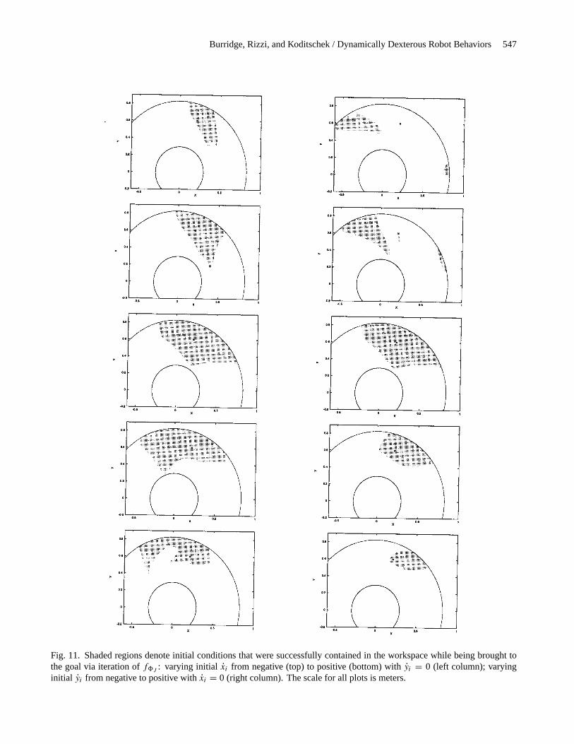
due to the decoupling ofH andV discussed in Section 2.5).In Figure 11, we show samples of the “velocity spines” ofthese tests. In each plot, one initial velocity,hi , is chosen,and a range of positions is mapped forward under iterates off8. The shaded areas show the location of the first impactof all states that are successfully brought toG0 (denoted “∗”)without leaving the workspace serviced by the paddle. In theleft-hand column,yi = 0, while xi varies from large negativeto large positive. On the right side, the roles ofx and yare reversed. These plots demonstrate the rather complicatedshape of the domain of attraction, as we have tried to suggestintuitively in Figure 2.
4.1.1.D(8J0): The Domain of8J0
Currently, we have no convenient means of parameterizingthe true domain of8J0, pictured in Figure 11. Yet to buildthe sequential compositions suggested in this paper, we re-quire just such a parameterization of domains. Thus, we areled to find a smaller domain,D0, whose shape is more readilyrepresented, as introduced in Figure 1, and which is invari-ant with respect tof8J (i.e., f8J (D0) ⊂ D0). Ellipsoidsmake an obvious candidate shape, and have added appealfrom the analytical viewpoint. However, the ellipsoids wefind are considerably larger than those we have gotten in thepast from Lyapunov functions derived fromDf8J . Inclusionwithin an ellipsoid is also an easy test computationally—animportant consideration when many such tests must be doneevery update (currently 330 Hz).
To find an invariant ellipsoid, start with a candidate ellip-soid,Ntest ⊂ TH, centered atG0, and simulate one iterationof the return map,f8, to get the forward image of the ellipsoid,f8J (Ntest ). If f8J (Ntest ) ⊂ Ntest thenNtest is invariant un-derf8J . Otherwise, adjust the parameters of theNtest to ar-rive atN ′
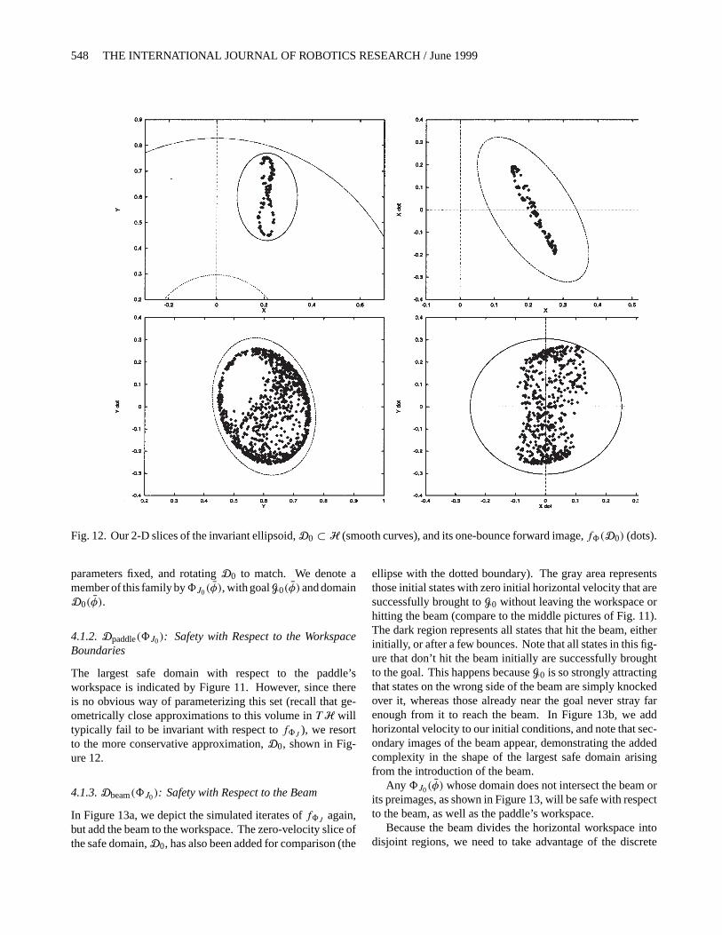
test , and repeat the process. In Figure 12, we displayfour slices through the surface of such an invariant ellipsoidfound after many trials (smooth ellipses), along with the sameslices of its single-iteration forward image (dots). Althoughthese pictures do not in themselves suffice to guarantee invari-ance, they provide a useful visualization of the domain andits forward image, and comprise the primary tool used in thesearch.11 The invariant ellipsoid depicted in Figure 12 willbe denotedD0 throughout the sequel.
Relying on the rotational symmetry of the mirror law, wenow use8J0 to create a family of controllers by varying onlythe angular component of the goal point,φ, keeping all other
11. SinceG0 is an attractor, the existence of open forward-invariant neigh-borhoods is guaranteed. However, “tuning the shape” ofNtest by hand canbe an arduous process. This process will be sped up enormously by accessto an analytically tractable return map. Even without analytical results, thesearch for invariance could be automated by recourse to positive-definiteprogramming (a convex nonlinear programming problem) on the parameters(in this case, the entries of a positive-definite matrix) defining the shape ofthe invariant set. We are presently exploring this approach to generation ofNtest .
Burridge, Rizzi, and Koditschek / Dynamically Dexterous Robot Behaviors 547
Fig. 11. Shaded regions denote initial conditions that were successfully contained in the workspace while being brought tothe goal via iteration off8J : varying initial xi from negative (top) to positive (bottom) withyi = 0 (left column); varyinginitial yi from negative to positive withxi = 0 (right column). The scale for all plots is meters.
548 THE INTERNATIONAL JOURNAL OF ROBOTICS RESEARCH / June 1999
Fig. 12. Our 2-D slices of the invariant ellipsoid,D0 ⊂ H (smooth curves), and its one-bounce forward image,f8(D0) (dots).
parameters fixed, and rotatingD0 to match. We denote amember of this family by8J0(φ), with goalG0(φ)and domainD0(φ).
4.1.2.Dpaddle(8J0): Safety with Respect to the WorkspaceBoundaries
The largest safe domain with respect to the paddle’sworkspace is indicated by Figure 11. However, since thereis no obvious way of parameterizing this set (recall that ge-ometrically close approximations to this volume inTH willtypically fail to be invariant with respect tof8J ), we resortto the more conservative approximation,D0, shown in Fig-ure 12.
4.1.3.Dbeam(8J0): Safety with Respect to the Beam
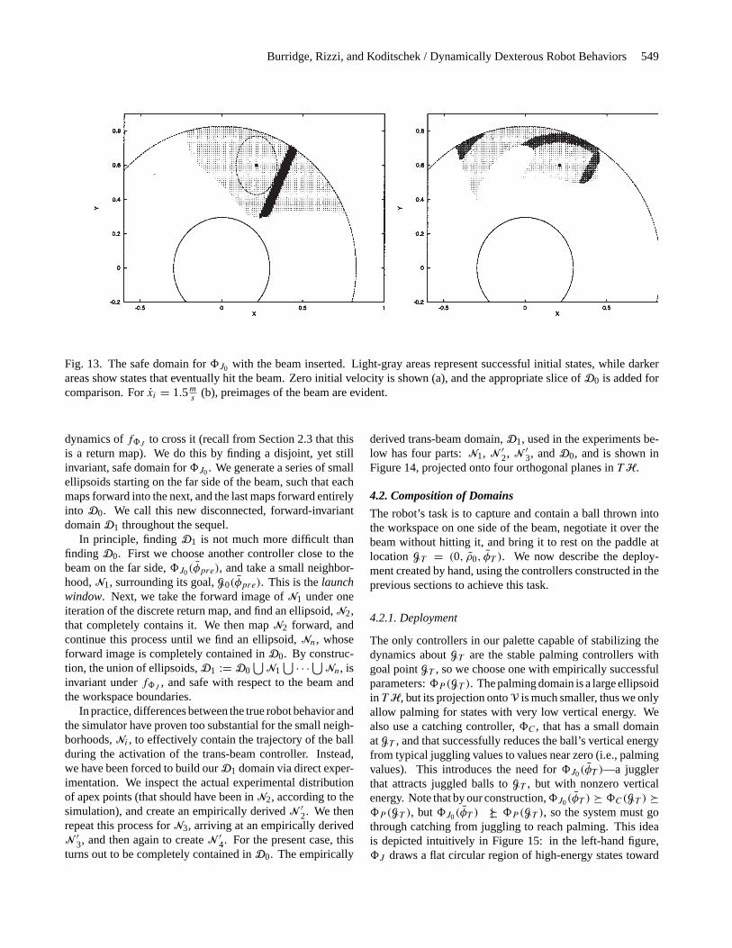
In Figure 13a, we depict the simulated iterates off8J again,but add the beam to the workspace. The zero-velocity slice ofthe safe domain,D0, has also been added for comparison (the
ellipse with the dotted boundary). The gray area representsthose initial states with zero initial horizontal velocity that aresuccessfully brought toG0 without leaving the workspace orhitting the beam (compare to the middle pictures of Fig. 11).The dark region represents all states that hit the beam, eitherinitially, or after a few bounces. Note that all states in this fig-ure that don’t hit the beam initially are successfully broughtto the goal. This happens becauseG0 is so strongly attractingthat states on the wrong side of the beam are simply knockedover it, whereas those already near the goal never stray farenough from it to reach the beam. In Figure 13b, we addhorizontal velocity to our initial conditions, and note that sec-ondary images of the beam appear, demonstrating the addedcomplexity in the shape of the largest safe domain arisingfrom the introduction of the beam.
Any8J0(φ) whose domain does not intersect the beam orits preimages, as shown in Figure 13, will be safe with respectto the beam, as well as the paddle’s workspace.
Because the beam divides the horizontal workspace intodisjoint regions, we need to take advantage of the discrete
Burridge, Rizzi, and Koditschek / Dynamically Dexterous Robot Behaviors 549
Fig. 13. The safe domain for8J0 with the beam inserted. Light-gray areas represent successful initial states, while darkerareas show states that eventually hit the beam. Zero initial velocity is shown (a), and the appropriate slice ofD0 is added forcomparison. Forxi = 1.5m
s(b), preimages of the beam are evident.
dynamics off8J to cross it (recall from Section 2.3 that thisis a return map). We do this by finding a disjoint, yet stillinvariant, safe domain for8J0. We generate a series of smallellipsoids starting on the far side of the beam, such that eachmaps forward into the next, and the last maps forward entirelyinto D0. We call this new disconnected, forward-invariantdomainD1 throughout the sequel.
In principle, findingD1 is not much more difficult thanfinding D0. First we choose another controller close to thebeam on the far side,8J0(φpre), and take a small neighbor-hood,N1, surrounding its goal,G0(φpre). This is thelaunchwindow. Next, we take the forward image ofN1 under oneiteration of the discrete return map, and find an ellipsoid,N2,that completely contains it. We then mapN2 forward, andcontinue this process until we find an ellipsoid,Nn, whoseforward image is completely contained inD0. By construc-tion, the union of ellipsoids,D1 := D0
⋃N1
⋃ · · · ⋃ Nn, isinvariant underf8J , and safe with respect to the beam andthe workspace boundaries.
In practice, differences between the true robot behavior andthe simulator have proven too substantial for the small neigh-borhoods,Ni , to effectively contain the trajectory of the ballduring the activation of the trans-beam controller. Instead,we have been forced to build ourD1 domain via direct exper-imentation. We inspect the actual experimental distributionof apex points (that should have been inN2, according to thesimulation), and create an empirically derivedN ′
2. We thenrepeat this process forN3, arriving at an empirically derivedN ′
3, and then again to createN ′4. For the present case, this
turns out to be completely contained inD0. The empirically
derived trans-beam domain,D1, used in the experiments be-low has four parts:N1, N ′
2, N ′3, andD0, and is shown in
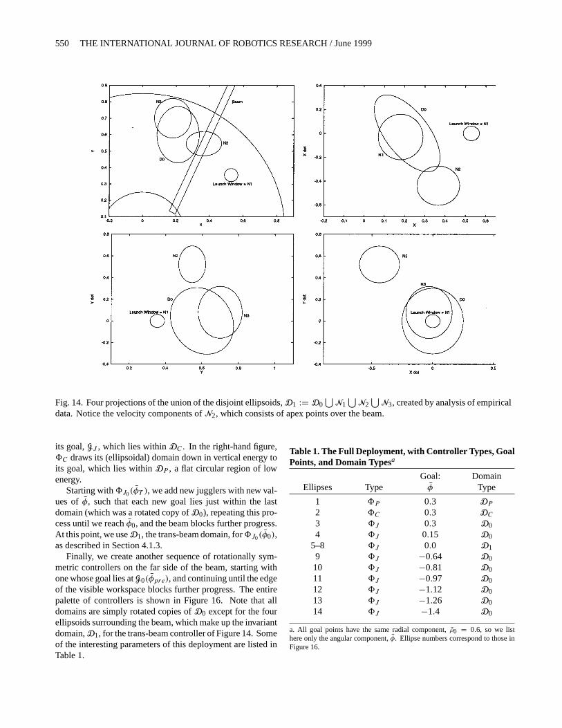
Figure 14, projected onto four orthogonal planes inTH.
4.2. Composition of Domains
The robot’s task is to capture and contain a ball thrown intothe workspace on one side of the beam, negotiate it over thebeam without hitting it, and bring it to rest on the paddle atlocation GT = (0, ρ0, φT ). We now describe the deploy-ment created by hand, using the controllers constructed in theprevious sections to achieve this task.
4.2.1. Deployment
The only controllers in our palette capable of stabilizing thedynamics aboutGT are the stable palming controllers withgoal pointGT , so we choose one with empirically successfulparameters:8P (GT ). The palming domain is a large ellipsoidin TH, but its projection ontoV is much smaller, thus we onlyallow palming for states with very low vertical energy. Wealso use a catching controller,8C , that has a small domainatGT , and that successfully reduces the ball’s vertical energyfrom typical juggling values to values near zero (i.e., palmingvalues). This introduces the need for8J0(φT )—a jugglerthat attracts juggled balls toGT , but with nonzero verticalenergy. Note that by our construction,8J0(φT ) � 8C(GT ) �8P (GT ), but8J0(φT ) |� 8P (GT ), so the system must gothrough catching from juggling to reach palming. This ideais depicted intuitively in Figure 15: in the left-hand figure,8J draws a flat circular region of high-energy states toward
550 THE INTERNATIONAL JOURNAL OF ROBOTICS RESEARCH / June 1999
Fig. 14. Four projections of the union of the disjoint ellipsoids,D1 := D0⋃
N1⋃
N2⋃
N3, created by analysis of empiricaldata. Notice the velocity components ofN2, which consists of apex points over the beam.
its goal,GJ , which lies withinDC . In the right-hand figure,8C draws its (ellipsoidal) domain down in vertical energy toits goal, which lies withinDP , a flat circular region of lowenergy.
Starting with8J0(φT ), we add new jugglers with new val-ues of φ, such that each new goal lies just within the lastdomain (which was a rotated copy ofD0), repeating this pro-cess until we reachφ0, and the beam blocks further progress.At this point, we useD1, the trans-beam domain, for8J0(φ0),as described in Section 4.1.3.
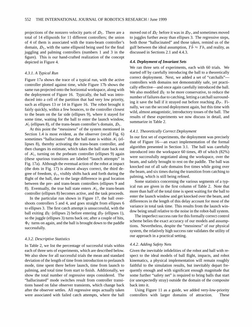
Finally, we create another sequence of rotationally sym-metric controllers on the far side of the beam, starting withone whose goal lies atG0(φpre), and continuing until the edgeof the visible workspace blocks further progress. The entirepalette of controllers is shown in Figure 16. Note that alldomains are simply rotated copies ofD0 except for the fourellipsoids surrounding the beam, which make up the invariantdomain,D1, for the trans-beam controller of Figure 14. Someof the interesting parameters of this deployment are listed inTable 1.
Table 1. The Full Deployment, with Controller Types, GoalPoints, and Domain Typesa
Goal: DomainEllipses Type φ Type
1 8P 0.3 DP
2 8C 0.3 DC
3 8J 0.3 D04 8J 0.15 D0
5–8 8J 0.0 D19 8J −0.64 D010 8J −0.81 D011 8J −0.97 D012 8J −1.12 D013 8J −1.26 D014 8J −1.4 D0
a. All goal points have the same radial component,ρ0 = 0.6, so we listhere only the angular component,φ. Ellipse numbers correspond to those inFigure 16.
Burridge, Rizzi, and Koditschek / Dynamically Dexterous Robot Behaviors 551
Fig. 15. Juggle to catch to palm: the juggle drives all of its domain toGJ , which lies within the domain for the catch, but withnonzero vertical energy (a); the catch reduces the vertical energy of the ball, bringing it down into the domain for palming (b).
Fig. 16. A theoretically sound deployment using the jumpcontroller of Figure 14.
Every member of this deployment was chosen by hand toensure that a path exists from all the domains to the task goalstate. The algorithm of Section 3.1 leads in a straightforwardmanner to a linear tree with no branches, thus the ideal tra-jectory of the system should be a stepwise descent from thefirst cell of the partition entered through all the intermediatecells, and finally to the catching and then to the palming cell,where it should remain.
4.2.2. A Hierarchy of Controllers
The deployment and controller-switching scheme we havejust described relies for its formal properties on the abstracteddomain and goal properties of the constituent return maps. In
turn, the invariance and attracting properties off8 arise fromabstractions whose validity depends on the underlying track-ing and convergence properties of the continuous controllerand observer. Thus, we have a hierarchy of controllers (and,hence, of abstraction), where each level functions on the basisof certain assumptions about the quality of performance of thelower levels. As we see in Section 4.4.3, however, there willbe situations where the transients in the robot’s tracking ofthe reference are too large for it to get to the ball despite themirror law, thus violating the underlying assumptions at thelower level. Moreover, we see in Section 4.3 that the noise inthe system sometimes causes the ball to stray from all the do-mains of the deployment, despite their theoretical invariance,violating the properties assumed by the higher level.
The entire deployment of Section 4.2.1 may be thought ofas generating a single (complex) controller,8, with its owngoal and domain, which could be used as an element of a stillmore complex deployment. When this is done, there will beassumptions about the ability of8 to safely move the ballacross the beam and to its goal, and so the process continues.
In summary, a hierarchical system will function only aswell as its constituent abstractions can be realized empirically.Since no model is ever perfect, all theoretical guarantees aresubject to operating assumptions. It is important to keep inmind the lower-level assumptions being made, so that empir-ical settings wherein such assumptions fail can be identified.
4.3. Characteristics of the Test Runs
In Figure 16, we depict the entire deployment of the previoussection by superimposing the zero-velocity slices of all thevarious domains onto the horizontal workspace, along with
552 THE INTERNATIONAL JOURNAL OF ROBOTICS RESEARCH / June 1999
projections of the nonzero velocity parts ofD1. There are atotal of 14 ellipsoids for 11 different controllers; the unionof 4 of them is associated with the trans-beam controller’sdomain,D1, with the same ellipsoid being used for the finaljuggling and palming controllers (numbers 1 and 3 in thefigure). This is our hand-crafted realization of the conceptdepicted in Figure 4.
4.3.1. A Typical Run
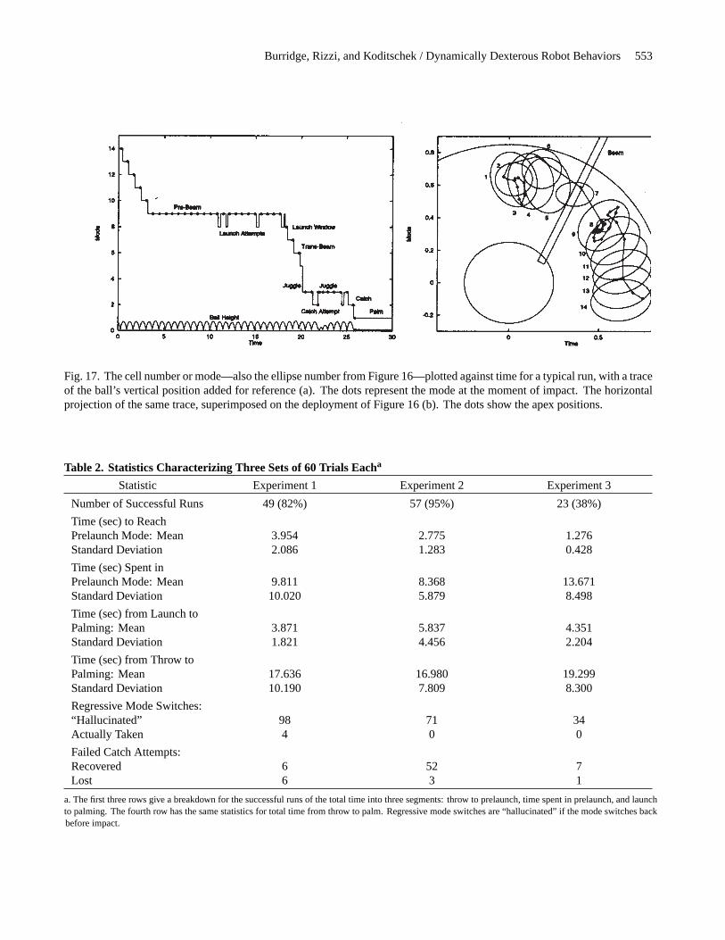
Figure 17a shows the trace of a typical run, with the activecontroller plotted against time, while Figure 17b shows thesame run projected onto the horizontal workspace, along withthe deployment of Figure 16. Typically, the ball was intro-duced into a cell of the partition that had very low priority,such as ellipses 13 or 14 in Figure 16. The robot brought itfairly quickly, within a few bounces, to the controller closestto the beam on the far side (ellipses 9), where it stayed forsome time, waiting for the ball to enter the launch window,N1 (ellipses 8), of the trans-beam controller’s domain,D1.
At this point the “messiness” of the system mentioned inSection 1.4 is most evident, as the observer (recall Fig. 6)sometimes “hallucinates” that the ball state is withinN1 (el-lipses 8), thereby activating the trans-beam controller, andthen changes its estimate, which takes the ball state back outof N1, turning on the prebeam controller (ellipses 9) again(these spurious transitions are labeled “launch attempts” inFig. 17a). Although the eventual action of the robot at impact(the dots in Fig. 17) is almost always correct, the third de-gree of freedom,ψr , visibly shifts back and forth during theflight of the ball, due to the large difference in goal locationbetween the pre- and trans-beam controllers (ellipses 9 and8). Eventually, the true ball state entersN1, the trans-beamcontroller (ellipses 8) becomes active, and the task proceeds.
In the particular run shown in Figure 17, the ball over-shoots controllers 5 and 4, and goes straight from ellipses 6to ellipses 3. The first catch attempt is unsuccessful, with theball exitingDC (ellipses 2) before enteringDP (ellipses 1),so the juggle (ellipses 3) turns back on; after a couple of hits,8C turns on again, and the ball is brought down to the paddlesuccessfully.
4.3.2. Descriptive Statistics
In Table 2, we list the percentage of successful trials withineach of three sets of experiments, which are described below.We also show for all successful trials the mean and standarddeviation of the length of time from introduction to prelaunchmode, time spent there before launch, time from launch topalming, and total time from start to finish. Additionally, weshow the total number of regressive steps considered. The“hallucinated” mode switches result from controller transi-tions based on false observer transients, which change backafter the observer settles. All regressive steps actually takenwere associated with failed catch attempts, where the ball
moved out ofDC before it was inDP , and sometimes movedto juggles further away than ellipses 3. The regressive steps,both those “hallucinated” and those taken, remind us of thegulf between the ideal assumption,T b ≈ T b, and reality, asdiscussed in Sections 2.1 and 4.4.3.
4.4. Deployment of Invariant SetsWe ran three sets of experiments, each with 60 trials. Westarted off by carefully introducing the ball to a theoreticallycorrect deployment. Next, we added a set of “catchalls”—controllers with domains not demonstrably safe, yet practi-cally effective—and once again carefully introduced the ball.We also modifiedDC to be more conservative, to reduce thenumber of failures due to catching, letting a catchall surround-ing it save the ball if it strayed out before reachingDP . Fi-nally, we ran the second deployment again, but this time withwild, almost antagonistic, introductory tosses of the ball. Theresults of these experiments we now discuss in detail, andsummarize in Table 2.
4.4.1. Theoretically Correct Deployment
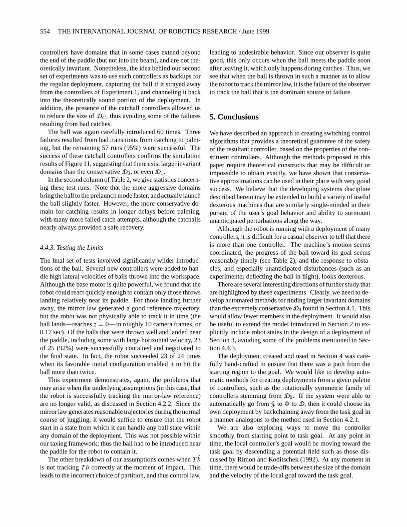
In our first set of experiments, the deployment was preciselythat of Figure 16—an exact implementation of the formalalgorithm presented in Section 3.1. The ball was carefullyintroduced into the workspace 60 times, 49 of which (82%)were successfully negotiated along the workspace, over thebeam, and safely brought to rest on the paddle. The ball wasknocked out of all safe domains five times while going overthe beam, and six times during the transition from catching topalming, which is still being refined.
Some statistics concerning the various segments of a typ-ical run are given in the first column of Table 2. Note thatmore than half of the total time is spent waiting for the ball toenter the launch window and get knocked over the beam, anddifferences in the length of this delay account for most of thevariance in total task time. This results from the launch win-dow being small relative to the noise in the robot-ball system.
The imperfect success rate for this formally correct controlscheme belies the exact accuracy of our models and assump-tions. Nevertheless, despite the “messiness” of our physicalsystem, the relatively high success rate validates the utility ofour approach in a practical setting.
4.4.2. Adding Safety Nets
Given the inevitable infidelities of the robot and ball with re-spect to the ideal models of ball flight, impacts, and robotkinematics, a physical implementation will remain roughlyfaithful to the simulation results, but inevitably depart fre-quently enough and with significant enough magnitude thatsome further “safety net” is required to bring balls that start(or unexpectedly stray) outside the domain of the compositeback into it.
Using Figure 11 as a guide, we added very-low-prioritycontrollers with larger domains of attraction. These
Burridge, Rizzi, and Koditschek / Dynamically Dexterous Robot Behaviors 553
Fig. 17. The cell number or mode—also the ellipse number from Figure 16—plotted against time for a typical run, with a traceof the ball’s vertical position added for reference (a). The dots represent the mode at the moment of impact. The horizontalprojection of the same trace, superimposed on the deployment of Figure 16 (b). The dots show the apex positions.
Table 2. Statistics Characterizing Three Sets of 60 Trials Eacha
Statistic Experiment 1 Experiment 2 Experiment 3
Number of Successful Runs 49 (82%) 57 (95%) 23 (38%)
Time (sec) to ReachPrelaunch Mode: Mean 3.954 2.775 1.276Standard Deviation 2.086 1.283 0.428
Time (sec) Spent inPrelaunch Mode: Mean 9.811 8.368 13.671Standard Deviation 10.020 5.879 8.498
Time (sec) from Launch toPalming: Mean 3.871 5.837 4.351Standard Deviation 1.821 4.456 2.204
Time (sec) from Throw toPalming: Mean 17.636 16.980 19.299Standard Deviation 10.190 7.809 8.300
Regressive Mode Switches:“Hallucinated” 98 71 34Actually Taken 4 0 0
Failed Catch Attempts:Recovered 6 52 7Lost 6 3 1
a. The first three rows give a breakdown for the successful runs of the total time into three segments: throw to prelaunch, time spent in prelaunch, and launchto palming. The fourth row has the same statistics for total time from throw to palm. Regressive mode switches are “hallucinated” if the mode switches backbefore impact.
554 THE INTERNATIONAL JOURNAL OF ROBOTICS RESEARCH / June 1999
controllers have domains that in some cases extend beyondthe end of the paddle (but not into the beam), and are not the-oretically invariant. Nonetheless, the idea behind our secondset of experiments was to use such controllers as backups forthe regular deployment, capturing the ball if it strayed awayfrom the controllers of Experiment 1, and channeling it backinto the theoretically sound portion of the deployment. Inaddition, the presence of the catchall controllers allowed usto reduce the size ofDC , thus avoiding some of the failuresresulting from bad catches.
The ball was again carefully introduced 60 times. Threefailures resulted from bad transitions from catching to palm-ing, but the remaining 57 runs (95%) were successful. Thesuccess of these catchall controllers confirms the simulationresults of Figure 11, suggesting that there exist larger invariantdomains than the conservativeD0, or evenD1.
In the second column of Table 2, we give statistics concern-ing these test runs. Note that the more aggressive domainsbring the ball to the prelaunch mode faster, and actually launchthe ball slightly faster. However, the more conservative do-main for catching results in longer delays before palming,with many more failed catch attempts, although the catchallsnearly always provided a safe recovery.
4.4.3. Testing the Limits
The final set of tests involved significantly wilder introduc-tions of the ball. Several new controllers were added to han-dle high lateral velocities of balls thrown into the workspace.Although the base motor is quite powerful, we found that therobot could react quickly enough to contain only those throwslanding relatively near its paddle. For those landing furtheraway, the mirror law generated a good reference trajectory,but the robot was not physically able to track it in time (theball lands—reachesz = 0—in roughly 10 camera frames, or0.17 sec). Of the balls that were thrown well and landed nearthe paddle, including some with large horizontal velocity, 23of 25 (92%) were successfully contained and negotiated tothe final state. In fact, the robot succeeded 23 of 24 timeswhen its favorable initial configuration enabled it to hit theball more than twice.
This experiment demonstrates, again, the problems thatmay arise when the underlying assumptions (in this case, thatthe robot is successfully tracking the mirror-law reference)are no longer valid, as discussed in Section 4.2.2. Since themirror law generates reasonable trajectories during the normalcourse of juggling, it would suffice to ensure that the robotstart in a state from which it can handle any ball state withinany domain of the deployment. This was not possible withinour taxing framework; thus the ball had to be introduced nearthe paddle for the robot to contain it.
The other breakdown of our assumptions comes whenT b
is not trackingT b correctly at the moment of impact. Thisleads to the incorrect choice of partition, and thus control law,
leading to undesirable behavior. Since our observer is quitegood, this only occurs when the ball meets the paddle soonafter leaving it, which only happens during catches. Thus, wesee that when the ball is thrown in such a manner as to allowthe robot to track the mirror law, it is the failure of the observerto track the ball that is the dominant source of failure.
5. Conclusions
We have described an approach to creating switching controlalgorithms that provides a theoretical guarantee of the safetyof the resultant controller, based on the properties of the con-stituent controllers. Although the methods proposed in thispaper require theoretical constructs that may be difficult orimpossible to obtain exactly, we have shown that conserva-tive approximations can be used in their place with very goodsuccess. We believe that the developing systems disciplinedescribed herein may be extended to build a variety of usefuldexterous machines that are similarly single-minded in theirpursuit of the user’s goal behavior and ability to surmountunanticipated perturbations along the way.
Although the robot is running with a deployment of manycontrollers, it is difficult for a casual observer to tell that thereis more than one controller. The machine’s motion seemscoordinated, the progress of the ball toward its goal seemsreasonably timely (see Table 2), and the response to obsta-cles, and especially unanticipated disturbances (such as anexperimenter deflecting the ball in flight), looks dexterous.
There are several interesting directions of further study thatare highlighted by these experiments. Clearly, we need to de-velop automated methods for finding larger invariant domainsthan the extremely conservativeD0 found in Section 4.1. Thiswould allow fewer members in the deployment. It would alsobe useful to extend the model introduced in Section 2 to ex-plicitly include robot states in the design of a deployment ofSection 3, avoiding some of the problems mentioned in Sec-tion 4.4.3.
The deployment created and used in Section 4 was care-fully hand-crafted to ensure that there was a path from thestarting region to the goal. We would like to develop auto-matic methods for creating deployments from a given paletteof controllers, such as the rotationally symmetric family ofcontrollers stemming fromD0. If the system were able toautomatically go fromG to8 to D, then it could choose itsown deployment by backchaining away from the task goal ina manner analogous to the method used in Section 4.2.1.
We are also exploring ways to move the controllersmoothly from starting point to task goal. At any point intime, the local controller’s goal would be moving toward thetask goal by descending a potential field such as those dis-cussed by Rimon and Koditschek (1992). At any moment intime, there would be trade-offs between the size of the domainand the velocity of the local goal toward the task goal.
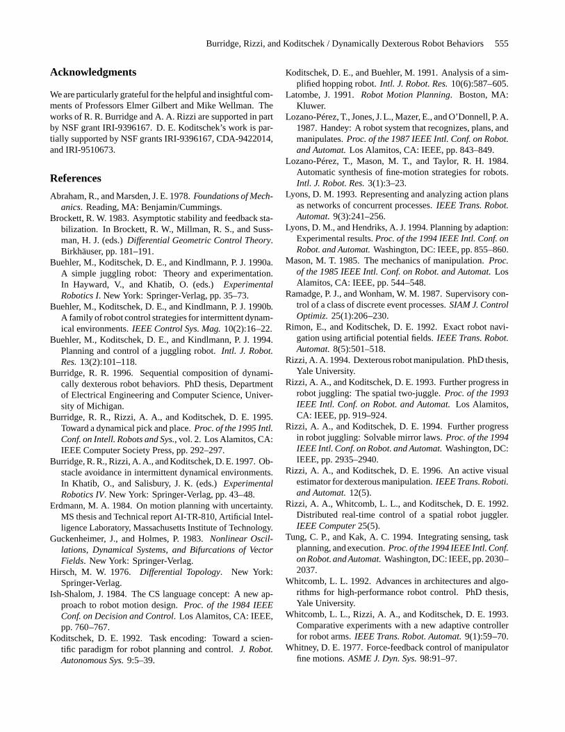
Burridge, Rizzi, and Koditschek / Dynamically Dexterous Robot Behaviors 555
Acknowledgments
We are particularly grateful for the helpful and insightful com-ments of Professors Elmer Gilbert and Mike Wellman. Theworks of R. R. Burridge and A. A. Rizzi are supported in partby NSF grant IRI-9396167. D. E. Koditschek’s work is par-tially supported by NSF grants IRI-9396167, CDA-9422014,and IRI-9510673.
References
Abraham, R., and Marsden, J. E. 1978.Foundations of Mech-anics. Reading, MA: Benjamin/Cummings.
Brockett, R. W. 1983. Asymptotic stability and feedback sta-bilization. In Brockett, R. W., Millman, R. S., and Suss-man, H. J. (eds.)Differential Geometric Control Theory.Birkhäuser, pp. 181–191.
Buehler, M., Koditschek, D. E., and Kindlmann, P. J. 1990a.A simple juggling robot: Theory and experimentation.In Hayward, V., and Khatib, O. (eds.)ExperimentalRobotics I. New York: Springer-Verlag, pp. 35–73.
Buehler, M., Koditschek, D. E., and Kindlmann, P. J. 1990b.A family of robot control strategies for intermittent dynam-ical environments.IEEE Control Sys. Mag.10(2):16–22.
Buehler, M., Koditschek, D. E., and Kindlmann, P. J. 1994.Planning and control of a juggling robot.Intl. J. Robot.Res.13(2):101–118.
Burridge, R. R. 1996. Sequential composition of dynami-cally dexterous robot behaviors. PhD thesis, Departmentof Electrical Engineering and Computer Science, Univer-sity of Michigan.
Burridge, R. R., Rizzi, A. A., and Koditschek, D. E. 1995.Toward a dynamical pick and place.Proc. of the 1995 Intl.Conf. on Intell. Robots and Sys., vol. 2. Los Alamitos, CA:IEEE Computer Society Press, pp. 292–297.
Burridge, R. R., Rizzi, A. A., and Koditschek, D. E. 1997. Ob-stacle avoidance in intermittent dynamical environments.In Khatib, O., and Salisbury, J. K. (eds.)ExperimentalRobotics IV. New York: Springer-Verlag, pp. 43–48.
Erdmann, M. A. 1984. On motion planning with uncertainty.MS thesis and Technical report AI-TR-810, Artificial Intel-ligence Laboratory, Massachusetts Institute of Technology.
Guckenheimer, J., and Holmes, P. 1983.Nonlinear Oscil-lations, Dynamical Systems, and Bifurcations of VectorFields. New York: Springer-Verlag.
Hirsch, M. W. 1976. Differential Topology. New York:Springer-Verlag.
Ish-Shalom, J. 1984. The CS language concept: A new ap-proach to robot motion design.Proc. of the 1984 IEEEConf. on Decision and Control. Los Alamitos, CA: IEEE,pp. 760–767.
Koditschek, D. E. 1992. Task encoding: Toward a scien-tific paradigm for robot planning and control.J. Robot.Autonomous Sys.9:5–39.
Koditschek, D. E., and Buehler, M. 1991. Analysis of a sim-plified hopping robot.Intl. J. Robot. Res.10(6):587–605.
Latombe, J. 1991.Robot Motion Planning. Boston, MA:Kluwer.
Lozano-Pérez, T., Jones, J. L., Mazer, E., and O’Donnell, P. A.1987. Handey: A robot system that recognizes, plans, andmanipulates.Proc. of the 1987 IEEE Intl. Conf. on Robot.and Automat.Los Alamitos, CA: IEEE, pp. 843–849.
Lozano-Pérez, T., Mason, M. T., and Taylor, R. H. 1984.Automatic synthesis of fine-motion strategies for robots.Intl. J. Robot. Res.3(1):3–23.
Lyons, D. M. 1993. Representing and analyzing action plansas networks of concurrent processes.IEEE Trans. Robot.Automat.9(3):241–256.
Lyons, D. M., and Hendriks, A. J. 1994. Planning by adaption:Experimental results.Proc. of the 1994 IEEE Intl. Conf. onRobot. and Automat.Washington, DC: IEEE, pp. 855–860.
Mason, M. T. 1985. The mechanics of manipulation.Proc.of the 1985 IEEE Intl. Conf. on Robot. and Automat.LosAlamitos, CA: IEEE, pp. 544–548.
Ramadge, P. J., and Wonham, W. M. 1987. Supervisory con-trol of a class of discrete event processes.SIAM J. ControlOptimiz.25(1):206–230.
Rimon, E., and Koditschek, D. E. 1992. Exact robot navi-gation using artificial potential fields.IEEE Trans. Robot.Automat.8(5):501–518.
Rizzi, A. A. 1994. Dexterous robot manipulation. PhD thesis,Yale University.
Rizzi, A. A., and Koditschek, D. E. 1993. Further progress inrobot juggling: The spatial two-juggle.Proc. of the 1993IEEE Intl. Conf. on Robot. and Automat.Los Alamitos,CA: IEEE, pp. 919–924.
Rizzi, A. A., and Koditschek, D. E. 1994. Further progressin robot juggling: Solvable mirror laws.Proc. of the 1994IEEE Intl. Conf. on Robot. and Automat.Washington, DC:IEEE, pp. 2935–2940.
Rizzi, A. A., and Koditschek, D. E. 1996. An active visualestimator for dexterous manipulation.IEEE Trans. Roboti.and Automat.12(5).
Rizzi, A. A., Whitcomb, L. L., and Koditschek, D. E. 1992.Distributed real-time control of a spatial robot juggler.IEEE Computer25(5).
Tung, C. P., and Kak, A. C. 1994. Integrating sensing, taskplanning, and execution.Proc. of the 1994 IEEE Intl. Conf.on Robot. and Automat.Washington, DC: IEEE, pp. 2030–2037.
Whitcomb, L. L. 1992. Advances in architectures and algo-rithms for high-performance robot control. PhD thesis,Yale University.
Whitcomb, L. L., Rizzi, A. A., and Koditschek, D. E. 1993.Comparative experiments with a new adaptive controllerfor robot arms.IEEE Trans. Robot. Automat.9(1):59–70.
Whitney, D. E. 1977. Force-feedback control of manipulatorfine motions.ASME J. Dyn. Sys.98:91–97.