Embed Size (px)
Citation preview
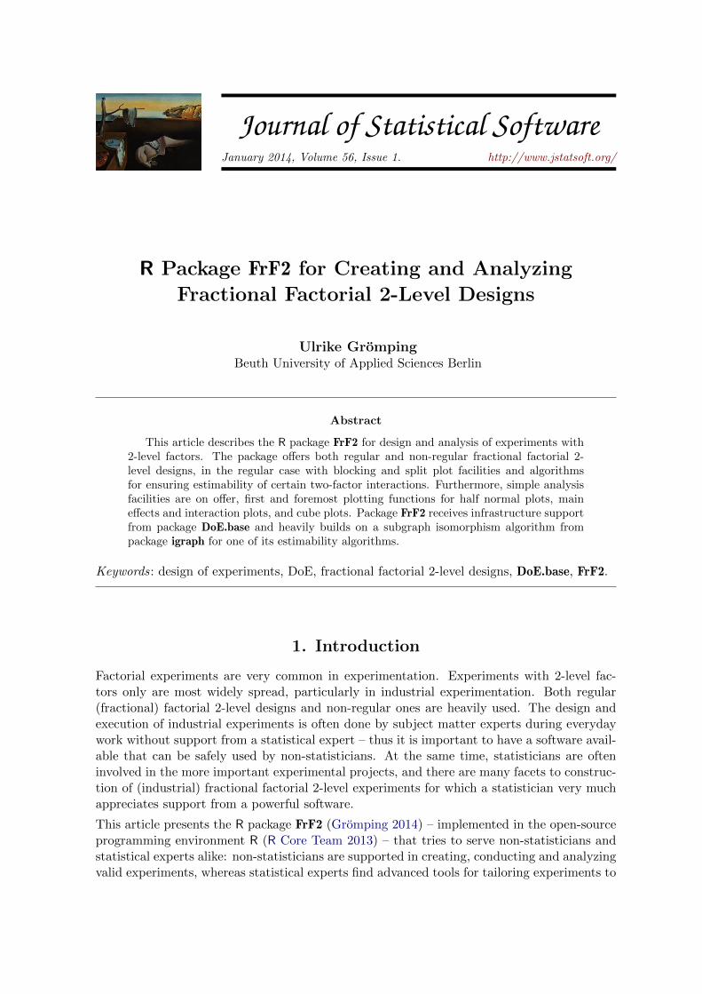
JSS Journal of Statistical SoftwareJanuary 2014, Volume 56, Issue 1. http://www.jstatsoft.org/
R Package FrF2 for Creating and Analyzing
Fractional Factorial 2-Level Designs
Ulrike GrompingBeuth University of Applied Sciences Berlin
Abstract
This article describes the R package FrF2 for design and analysis of experiments with2-level factors. The package offers both regular and non-regular fractional factorial 2-level designs, in the regular case with blocking and split plot facilities and algorithmsfor ensuring estimability of certain two-factor interactions. Furthermore, simple analysisfacilities are on offer, first and foremost plotting functions for half normal plots, maineffects and interaction plots, and cube plots. Package FrF2 receives infrastructure supportfrom package DoE.base and heavily builds on a subgraph isomorphism algorithm frompackage igraph for one of its estimability algorithms.
Keywords: design of experiments, DoE, fractional factorial 2-level designs, DoE.base, FrF2.
1. Introduction
Factorial experiments are very common in experimentation. Experiments with 2-level fac-tors only are most widely spread, particularly in industrial experimentation. Both regular(fractional) factorial 2-level designs and non-regular ones are heavily used. The design andexecution of industrial experiments is often done by subject matter experts during everydaywork without support from a statistical expert – thus it is important to have a software avail-able that can be safely used by non-statisticians. At the same time, statisticians are ofteninvolved in the more important experimental projects, and there are many facets to construc-tion of (industrial) fractional factorial 2-level experiments for which a statistician very muchappreciates support from a powerful software.
This article presents the R package FrF2 (Gromping 2014) – implemented in the open-sourceprogramming environment R (R Core Team 2013) – that tries to serve non-statisticians andstatistical experts alike: non-statisticians are supported in creating, conducting and analyzingvalid experiments, whereas statistical experts find advanced tools for tailoring experiments to

2 FrF2: Fractional Factorial 2-Level Designs in R
the specific needs of the experimental situation. R package FrF2 is part of a suite of severalR packages: DoE.base provides the infrastructure for the suite and creates general factorialdesigns, DoE.wrapper interfaces to other packages for design of experiments on the Compre-hensive R Archive Network (CRAN, http://CRAN.R-project.org/), and RcmdrPlugin.DoEprovides graphical user interface (GUI) access to the suite (Gromping 2013b,c,e, 2011b). Afifth package FrF2.catlg128 (Gromping 2013d) supports FrF2 for non-standard design creationtasks in 128 runs. These packages and all further packages on which they depend are availablefrom CRAN. The functionality implemented in FrF2 is discussed in this article, with occa-sional digressions into relevant functions from DoE.base and subsequent use of FrF2 designsby DoE.wrapper. The article provides an example-based discussion of the most importantfunctionality aspects, as well as of the general philosophy regarding input and output struc-ture. Details of algorithmic implementations are not covered, as this would exceed the scopeof one article.
R provides various further packages for creating and analyzing regular fractional factorial 2-level designs. An overview is given in the CRAN task view ”Design of Experiments (DoE) &Analysis of Experimental Data” (Gromping 2013a). Besides package FrF2 (Gromping 2014),R packages BHH2 (Barrios 2012a, companion package to Box, Hunter, and Hunter (2005)),BsMD (Barrios 2012b), qualityTools (Roth 2013) and planor (Kobilinsky, Bouvier, and Monod2013) also allow creation of fractional factorial 2-level designs, however with less comfort andautomatism: FrF2 is the only package that relies on a comprehensive catalogue of designs,automatically determines the overall best design or the best design for a certain estimationpurpose (option estimable) and offers automatic blocking and automatic creation of split plotdesigns. It should be mentioned here that the new package planor offers creation of regularfractional factorial designs not only for 2-level factors but also for factors at more than 2 levelsand mixed levels. planor appears to be more flexible than FrF2 regarding randomizationstructures; however, planor does not guarantee the quality criterion “minimum aberration”(see Section 3.1), is restricted to regular designs, offers less comfort and appears to be stillin an early implementation phase as an R package. Regarding analysis features, FrF2 offersvarious effects plots for fractional factorial 2-level designs. Packages BsMD and qualityToolsalso offer such functionality. One feature of BsMD is particularly noteworthy: it allowsto conduct the Box and Meyer (1993) Bayesian assessment of effects in a screening design;this methodology is uniquely implemented in that package, to the author’s knowledge; FrF2provides a function (BsProb.design) for convenient access to the methodology for designscreated with the package.
The remainder of this article is organized as follows: Section 2 briefly explains general ter-minology and important experimental principles, Section 3 presents the mathematical back-ground and terminology for fractional factorial 2-level designs. Section 4 provides two pub-lished examples that are used throughout the article for illustrating some design generationand analysis features. The implementation of regular fractional factorial 2-level designs infunction FrF2 is discussed in Section 5, while simple analysis tools are presented in Section 6.Design and analysis of non-regular fractional factorial 2-level designs is discussed in Section 7.Section 8 gives a brief overview of tools for augmenting or combining fractional factorial 2-leveldesigns. Finally, a brief overview of interesting topics not covered in this article is provided.Appendix A provides some information on the class design (as far as relevant for fractionalfactorial 2-level designs), Appendix B discusses data export and import utilities provided byDoE.base, Appendix C gives details on the class catlg for catalogues of fractional factorial
Journal of Statistical Software 3
2-level designs, and Appendix D provides details on the column orders used for screeningdesigns with function pb.
2. Basic terminology for experimentation
This section briefly explains basic terminology for experimental design, using full factorialplans as a starting point. The principle of replication is explained and distinguished fromrepeated measurements, and randomization and randomization restrictions are discussed.
This article defines an experimental design as a rectangular table each row of which containsa prescription for the settings of all design factors (columns) in a particular run of the experi-ment. An unreplicated full factorial 2-level design in k factors is an experimental design in 2k
runs (= experimental setups) that contains each possible level combination exactly once. Areplicated design contains each of its runs exactly r times, if r is the number of replications.It is helpful to distinguish between
� proper replications for which all sources of variability are newly set for the replicateruns,
� and repeated measurements, for which the settings of the experimental factors remainunchanged, and only the measurement process is repeated.
While proper replications are independent observations, it would be misleading to treat re-peated measurements as such.
Two important principles of experimentation are blocking and randomization. The scientificcommunity agrees that blocking should be used for keeping in check known influential factorsthat are not of interest in themselves (like batch variation), whereas randomization shouldbe used as a safeguard against bias from unknown influences (see e.g., Box et al. 2005, p. 93:“Block What You Can and Randomize What You Cannot”). For blocking a 2-level factorialexperiment, a block factor at two, four, eight, . . . levels is defined such that the known influ-ential factor can be kept constant within each block. For a useful experiment, the effect ofthe block factor need not be estimable itself, but can be aliased with other effects, as long asthose are not of interest either. The design and analysis usually assumes that block factorsdo not interact with experimental factors.
Randomization means that the experimental runs are conducted in random order; if the orderis completely randomized, all experimental runs can be treated as independent observations,and there is little risk of systematic bias from things like experimental order etc. For ablocked experiment, the experimental runs are randomized within each block only, which isa randomization restriction (blocks as a whole can also be randomized). Another random-ization restriction occurs in case of repeated measurements: they are usually not separatelyrandomized but conducted directly together, which is another way of distinguishing themfrom proper replications.
It can sometimes be necessary to keep some experimental factors fixed while changing others,mostly because of resource reasons. For example, when using a climate chamber for modifyingtwo environmental factors at two levels each, it will be impractical to conduct the runs inrandom order, readjusting the climate chamber after each run. Instead, one will want tocombine several runs with the same combination of levels of the environmental factors and
4 FrF2: Fractional Factorial 2-Level Designs in R
run them together, either in sequence or simultaneously, depending on the size and nature ofthe climate chamber. This is yet another type of randomization restriction: it is different fromthe blocking situation, since some factors of interest are kept fixed longer than the others.This situation is called a split plot design with so-called whole plot factors (the ones that arekept constant) and so-called split plot factors (the ones that change within whole plots). Forsplit plot designs, the runs within whole plots are randomized, and the order of the wholeplots is randomized. Split plot designs call for specific analysis strategies, e.g., mixed models.
3. Fractional factorial 2-level designs
This section provides the mathematical background for fractional factorial 2-level designs.There is a specific vocabulary that is reasonably straight-forward to grasp but may not beknown to all readers. Readers interested in more detail are referred to Mee (2009), Box et al.(2005) or Montgomery (2001), for example.
3.1. Regular fractional factorial 2-level designs
For regular fractional factorial 2-level designs in m factors, like for full factorial 2-level designs,the number of runs must be a power of 2, but it is only a fraction of the number of runs (2m)needed for a full factorial design (hence their name). Fractional factorial designs can alsobe replicated or run with repeated measurements and can also be completely randomizedor subject to randomization restrictions. (Replicating a fractional factorial design is notrecommended; it would usually be more useful to run a larger fraction without replication.)
The Yates matrix
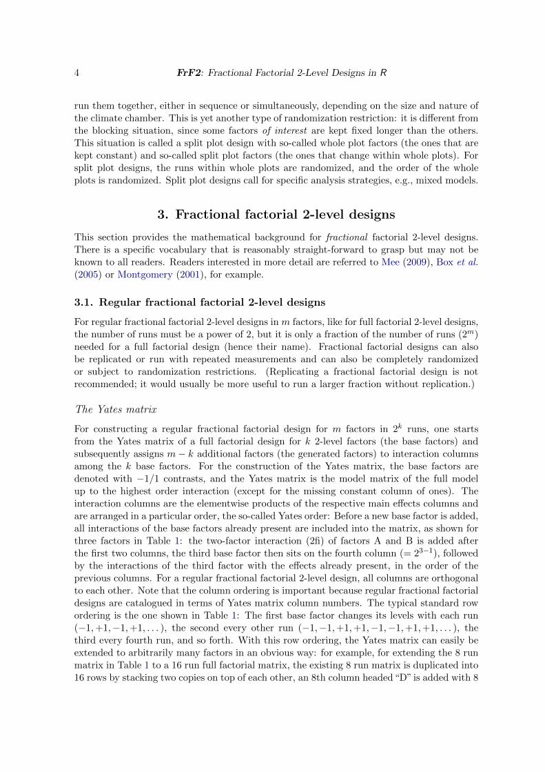
For constructing a regular fractional factorial design for m factors in 2k runs, one startsfrom the Yates matrix of a full factorial design for k 2-level factors (the base factors) andsubsequently assigns m− k additional factors (the generated factors) to interaction columnsamong the k base factors. For the construction of the Yates matrix, the base factors aredenoted with −1/1 contrasts, and the Yates matrix is the model matrix of the full modelup to the highest order interaction (except for the missing constant column of ones). Theinteraction columns are the elementwise products of the respective main effects columns andare arranged in a particular order, the so-called Yates order: Before a new base factor is added,all interactions of the base factors already present are included into the matrix, as shown forthree factors in Table 1: the two-factor interaction (2fi) of factors A and B is added afterthe first two columns, the third base factor then sits on the fourth column (= 23−1), followedby the interactions of the third factor with the effects already present, in the order of theprevious columns. For a regular fractional factorial 2-level design, all columns are orthogonalto each other. Note that the column ordering is important because regular fractional factorialdesigns are catalogued in terms of Yates matrix column numbers. The typical standard rowordering is the one shown in Table 1: The first base factor changes its levels with each run(−1,+1,−1,+1, . . . ), the second every other run (−1,−1,+1,+1,−1,−1,+1,+1, . . . ), thethird every fourth run, and so forth. With this row ordering, the Yates matrix can easily beextended to arbitrarily many factors in an obvious way: for example, for extending the 8 runmatrix in Table 1 to a 16 run full factorial matrix, the existing 8 run matrix is duplicated into16 rows by stacking two copies on top of each other, an 8th column headed“D” is added with 8
Journal of Statistical Software 5
A B AB C AC BC ABC
1 2 3 4 5 6 7
1 −1 −1 1 −1 1 1 −12 1 −1 −1 −1 −1 1 13 −1 1 −1 −1 1 −1 14 1 1 1 −1 −1 −1 −15 −1 −1 1 1 −1 −1 16 1 −1 −1 1 1 −1 −17 −1 1 −1 1 −1 1 −18 1 1 1 1 1 1 1
Table 1: Yates matrix for full factorial in 3 factors.
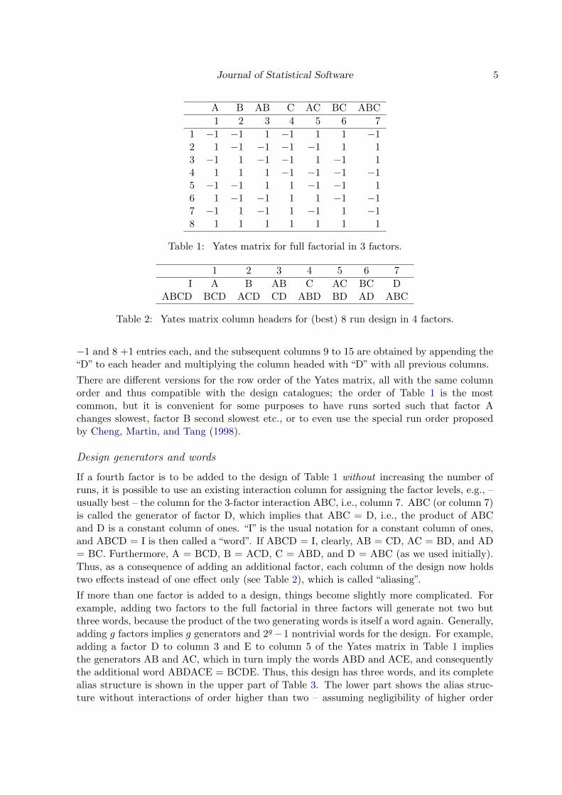
1 2 3 4 5 6 7
I A B AB C AC BC DABCD BCD ACD CD ABD BD AD ABC
Table 2: Yates matrix column headers for (best) 8 run design in 4 factors.
−1 and 8 +1 entries each, and the subsequent columns 9 to 15 are obtained by appending the“D” to each header and multiplying the column headed with “D” with all previous columns.
There are different versions for the row order of the Yates matrix, all with the same columnorder and thus compatible with the design catalogues; the order of Table 1 is the mostcommon, but it is convenient for some purposes to have runs sorted such that factor Achanges slowest, factor B second slowest etc., or to even use the special run order proposedby Cheng, Martin, and Tang (1998).
Design generators and words
If a fourth factor is to be added to the design of Table 1 without increasing the number ofruns, it is possible to use an existing interaction column for assigning the factor levels, e.g., –usually best – the column for the 3-factor interaction ABC, i.e., column 7. ABC (or column 7)is called the generator of factor D, which implies that ABC = D, i.e., the product of ABCand D is a constant column of ones. “I” is the usual notation for a constant column of ones,and ABCD = I is then called a “word”. If ABCD = I, clearly, AB = CD, AC = BD, and AD= BC. Furthermore, A = BCD, B = ACD, C = ABD, and D = ABC (as we used initially).Thus, as a consequence of adding an additional factor, each column of the design now holdstwo effects instead of one effect only (see Table 2), which is called “aliasing”.
If more than one factor is added to a design, things become slightly more complicated. Forexample, adding two factors to the full factorial in three factors will generate not two butthree words, because the product of the two generating words is itself a word again. Generally,adding g factors implies g generators and 2g−1 nontrivial words for the design. For example,adding a factor D to column 3 and E to column 5 of the Yates matrix in Table 1 impliesthe generators AB and AC, which in turn imply the words ABD and ACE, and consequentlythe additional word ABDACE = BCDE. Thus, this design has three words, and its completealias structure is shown in the upper part of Table 3. The lower part shows the alias struc-ture without interactions of order higher than two – assuming negligibility of higher order
6 FrF2: Fractional Factorial 2-Level Designs in R
1 2 3 4 5 6 7
I A B D C E BC CDABD BD AD AB AE AC DE BEACE CE CDE BCE BDE BCD ABE ABC
BCDE ABCDE ABCE ACDE ABCD ABDE ACD ADE
A B D C E BC CDBD AD AB AE AC DE BECE
Table 3: Yates matrix column headers for (best) 8 run design in 5 factors.
interactions. Such assumptions are often made and may be justified by a low order Taylorapproximation, if the experimental area is reasonably small. In the following, the k factorsoriginally spanning the 2k full factorial design are called the “base factors”, the g = m − kadditional factors are called the “generated factors”.
Simple analysis tools
Generally, results from (fractional) factorial 2-level designs can be analyzed using a linearmodel. With regular fractional factorial experiments, the model with all conceivable interac-tions is not estimable, because of perfect aliasing of some effects. Of course, the number ofestimable effects cannot exceed the number of different experimental runs. For example, thedesign of Table 2 allows estimation of the constant and the seven effects A+BCD, B+ACD,AB+CD, C+ABD, AC+BD, BC+AD and D+ABC. If one is prepared to assume negligibilityof 3-factor interactions, main effects can be estimated without bias in that design. For a validanalysis, it is of course absolutely crucial to be aware of the alias structure of a design.
Some assessment of significance is needed in order to distinguish random variation from realexperimental effects. For a design with proper replications, the estimable effects or effectsums can be tested for significance in the linear model. For unreplicated fractional factorialdesigns, significance tests from linear models often lack error degrees of freedom (dfs). Forsuch cases, as linear model analysis does not work well, plotting methods for assessing effectsignificance have been proposed (Daniel 1959; Lenth 1989). These work reasonably well underan assumption of effect sparsity: If the majority of effects is not active (i.e., has the expectedvalue zero), this non-active majority of effects can serve as an assessment of error variation.(Half) Normal plots of the effects show this majority of effects on a normality line and activeeffects as sticking out from that line. A half normal plot is often called Daniel plot, since itwas proposed by Daniel (1959); Lenth (1989) proposed a numerical method for assessing effectsignificance. There are also approaches different from the one by Lenth (1989), which are,however, not implemented in FrF2 and are therefore not discussed here. For an appropriateDaniel plot, it is crucial to include as many effects in the model as possible, i.e., as many asthere are columns in the Yates matrix. Daniel plots work better for larger than for smallerdesigns – often a design in 8 runs with only seven effects will not yield a clear picture.
For effect interpretation, simple effects plots (main effects and interaction plots that visualizeaverages for each level of one factor or for each combination of levels of two factors) are helpful;cube plots visualize the occasional 3-factor interaction. Of course, awareness of the aliasingstructure is again very important for drawing correct conclusions from any such plots.
Journal of Statistical Software 7
Word length pattern and resolution
The less aliasing there is in a design, the more effects can be estimated without bias risk. Theword list of a design summarizes all the aliasing that has been caused by adding g generatedfactors to the k base factors of the design. Words with three letters (= words of length 3)imply aliasing of main effects with 2fis; for example, the design in Table 3 has the wordABD, which implies confounding of the main effect of factor A with the BD interaction, andlikewise B with AD and D with AB. Words with four letters imply aliasing of main effectswith 3-factor interactions (3fis), and of 2fis with each other. Often, 3fis are assumed to benegligible, so that interest in 4-letter words results from their consequences for the aliasingof 2fis with each other (e.g., the word BCDE implies aliasing of BC with DE, of BD withCE and of BE with CD). Longer words have less severe consequences for usability of a designthan shorter words, if one is prepared to accept the rationale that low order effects like maineffects and 2fis are much more likely to be “active” than higher order effects.
It is customary to consider frequency tables of the word lengths of a design, the so-called“word length patterns” (WLPs): These are usually denoted as (A3, A4, . . . ). (Note thatthere cannot be words of length 2, because this would contradict orthogonality of the array.)For example, the WLPs for the designs of Tables 2 and 3 are (A3, A4, A5) = (0, 1, 0) and(A3, A4, A5) = (2, 1, 0). The length of the shortest word of a design is called the “resolution”of the design. Resolution is usually denoted in roman numerals and can be directly inferredfrom the WLP: it is the smallest word length with non-zero frequency. For example, thedesigns in Tables 2 and 3 have resolution IV and III, respectively.
Regular fractional factorial designs of resolution III are quite risky to use, because theyconfound main effects with 2fis: Even if interest is in main effects only, active 2fis can invalidateinference on these main effects. If the resolution is IV, main effects are no longer aliased with2fis and can be estimated without bias, as long as interactions of order three or higher arenegligible. However, 2fis can be aliased with each other. If all 2fis must be estimable (giventhat no effects of order three or higher exist), a design of resolution V is needed.
Minimum aberration
For larger designs, there are many different possibilities for adding g factors to an existingfull factorial in k base factors. Some of these possibilities are structurally identical (= “iso-morphic”), i.e., can be obtained from each other by swapping rows and/or columns and/orlevels within columns. A lot of work has been invested in cataloguing non-isomorphic designs.Existing catalogues assess the comparative quality of catalogued designs by comparing theirWLPs: a design D1 is better than a design D2, if it has smaller A3, or in case of equal A3
smaller A4 or . . . Thus, a design with higher resolution (see previous section) is always better,and in case of identical resolution, the word length pattern is successively minimized. Thiscriterion is called “minimum aberration” (MA). Within FrF2, a catalogue of non-isomorphicdesigns ordered by the minimum aberration criterion is available (see Section 3.2 for moredetail).
Maximum number of clear two-factor interactions, and MA clear designs
It has also been suggested to consider the number of “clear” 2fis as a quality criterion (Wuand Hamada 2000; Wu and Wu 2002). 2fis are called clear, if they are not aliased withmain effects or other 2fis (usually, this criterion is used for resolution IV and higher only).
8 FrF2: Fractional Factorial 2-Level Designs in R
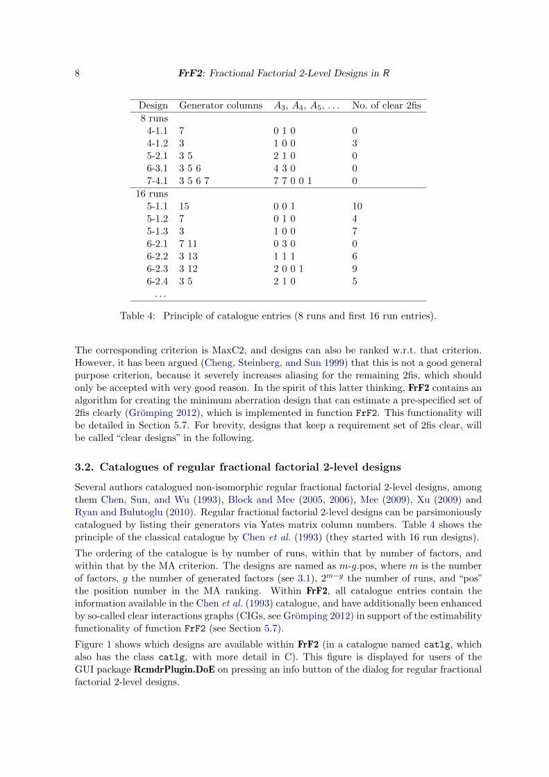
Design Generator columns A3, A4, A5, . . . No. of clear 2fis
8 runs4-1.1 7 0 1 0 04-1.2 3 1 0 0 35-2.1 3 5 2 1 0 06-3.1 3 5 6 4 3 0 07-4.1 3 5 6 7 7 7 0 0 1 0
16 runs5-1.1 15 0 0 1 105-1.2 7 0 1 0 45-1.3 3 1 0 0 76-2.1 7 11 0 3 0 06-2.2 3 13 1 1 1 66-2.3 3 12 2 0 0 1 96-2.4 3 5 2 1 0 5
. . .
Table 4: Principle of catalogue entries (8 runs and first 16 run entries).
The corresponding criterion is MaxC2, and designs can also be ranked w.r.t. that criterion.However, it has been argued (Cheng, Steinberg, and Sun 1999) that this is not a good generalpurpose criterion, because it severely increases aliasing for the remaining 2fis, which shouldonly be accepted with very good reason. In the spirit of this latter thinking, FrF2 contains analgorithm for creating the minimum aberration design that can estimate a pre-specified set of2fis clearly (Gromping 2012), which is implemented in function FrF2. This functionality willbe detailed in Section 5.7. For brevity, designs that keep a requirement set of 2fis clear, willbe called “clear designs” in the following.
3.2. Catalogues of regular fractional factorial 2-level designs
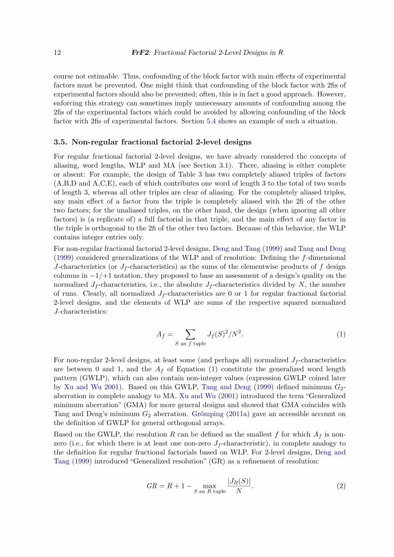
Several authors catalogued non-isomorphic regular fractional factorial 2-level designs, amongthem Chen, Sun, and Wu (1993), Block and Mee (2005, 2006), Mee (2009), Xu (2009) andRyan and Bulutoglu (2010). Regular fractional factorial 2-level designs can be parsimoniouslycatalogued by listing their generators via Yates matrix column numbers. Table 4 shows theprinciple of the classical catalogue by Chen et al. (1993) (they started with 16 run designs).
The ordering of the catalogue is by number of runs, within that by number of factors, andwithin that by the MA criterion. The designs are named as m-g.pos, where m is the numberof factors, g the number of generated factors (see 3.1), 2m−g the number of runs, and “pos”the position number in the MA ranking. Within FrF2, all catalogue entries contain theinformation available in the Chen et al. (1993) catalogue, and have additionally been enhancedby so-called clear interactions graphs (CIGs, see Gromping 2012) in support of the estimabilityfunctionality of function FrF2 (see Section 5.7).
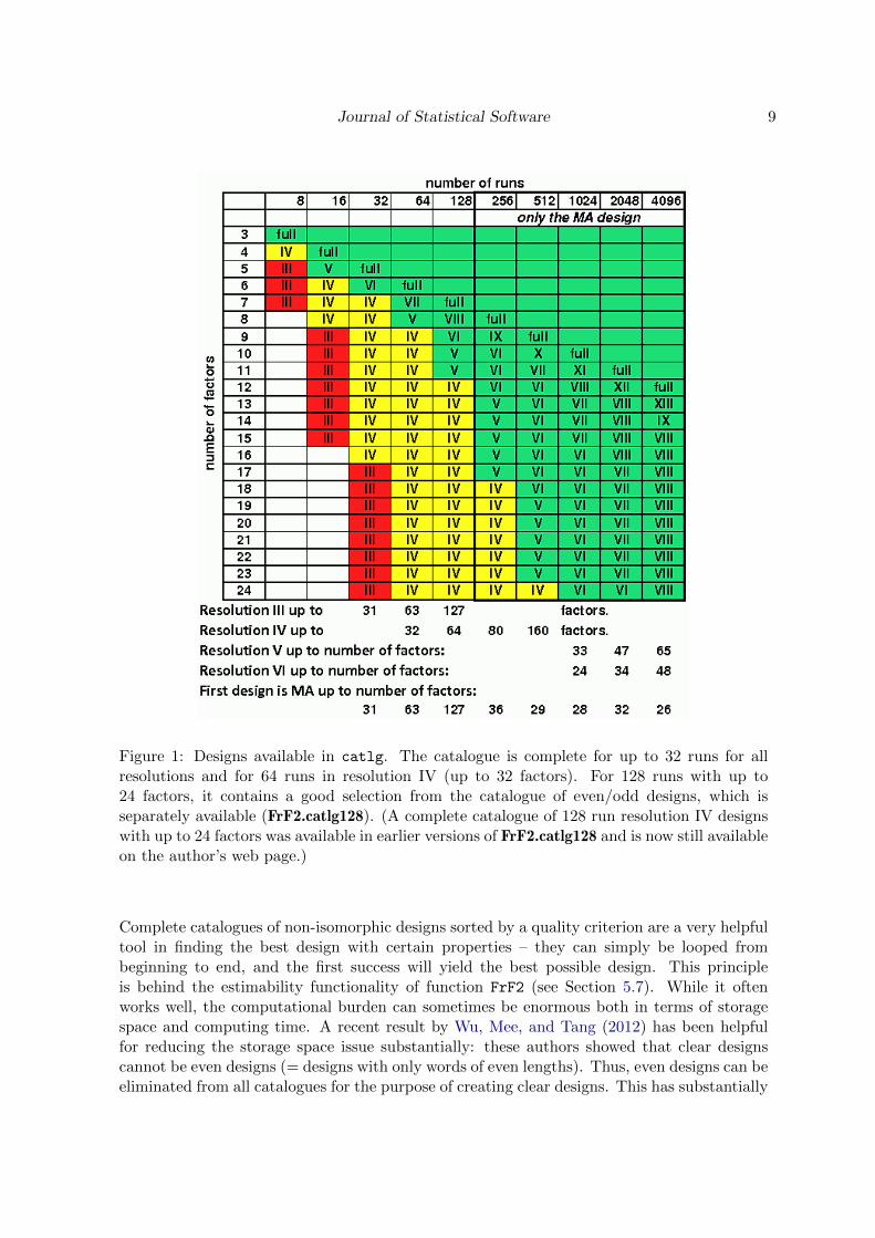
Figure 1 shows which designs are available within FrF2 (in a catalogue named catlg, whichalso has the class catlg, with more detail in C). This figure is displayed for users of theGUI package RcmdrPlugin.DoE on pressing an info button of the dialog for regular fractionalfactorial 2-level designs.
Journal of Statistical Software 9
Figure 1: Designs available in catlg. The catalogue is complete for up to 32 runs for allresolutions and for 64 runs in resolution IV (up to 32 factors). For 128 runs with up to24 factors, it contains a good selection from the catalogue of even/odd designs, which isseparately available (FrF2.catlg128). (A complete catalogue of 128 run resolution IV designswith up to 24 factors was available in earlier versions of FrF2.catlg128 and is now still availableon the author’s web page.)
Complete catalogues of non-isomorphic designs sorted by a quality criterion are a very helpfultool in finding the best design with certain properties – they can simply be looped frombeginning to end, and the first success will yield the best possible design. This principleis behind the estimability functionality of function FrF2 (see Section 5.7). While it oftenworks well, the computational burden can sometimes be enormous both in terms of storagespace and computing time. A recent result by Wu, Mee, and Tang (2012) has been helpfulfor reducing the storage space issue substantially: these authors showed that clear designscannot be even designs (= designs with only words of even lengths). Thus, even designs can beeliminated from all catalogues for the purpose of creating clear designs. This has substantially
10 FrF2: Fractional Factorial 2-Level Designs in R
Run size Max. number Run size Max. number
4 2 512 238 3 1024 33
16 5 2048 4732 6 4096 6564 8 8192 69
128 11 16384 92256 17 32768 120
Table 5: Maximum number of factors in resolution V regular fractional factorial 2-leveldesigns.
reduced the size of the 128 run catalogues in R package FrF2.catlg128. For the purpose offinding MA clear designs, further reduction to so-called dominating designs would be useful(introduced by Wu et al. 2012, who mainly concentrated on admissible designs). However, forother purposes, non-dominating designs might be interesting as well. Therefore, dominatingdesigns have only been flagged as such in order to speed up the search algorithm.
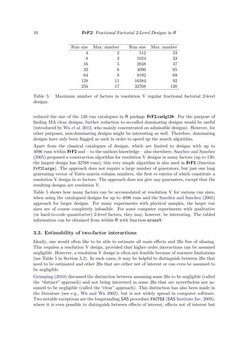
Apart from the classical catalogues of designs, which are limited to designs with up to4096 runs within FrF2 and – to the authors knowledge – also elsewhere, Sanchez and Sanchez(2005) proposed a construction algorithm for resolution V designs in many factors (up to 120;the largest design has 32768 runs); this very simple algorithm is also used in FrF2 (functionFrF2Large). The approach does not require a large number of generators, but just one longgenerating vector of Yates matrix column numbers, the first m entries of which constitute aresolution V design in m factors. The approach does not give any guarantees, except that theresulting designs are resolution V.
Table 5 shows how many factors can be accomodated at resolution V for various run sizes,when using the catalogued designs for up to 4096 runs and the Sanchez and Sanchez (2005)approach for larger designs. For many experiments with physical samples, the larger runsizes are of course completely infeasible. For some computer experiments with qualitative(or hard-to-code quantitative) 2-level factors, they may, however, be interesting. The tabledinformation can be obtained from within R with function nrunsV.
3.3. Estimability of two-factor interactions
Ideally, one would often like to be able to estimate all main effects and 2fis free of aliasing.This requires a resolution V design, provided that higher order interactions can be assumednegligible. However, a resolution V design is often not feasible because of resource limitations(see Table 5 in Section 3.2). In such cases, it may be helpful to distinguish between 2fis thatneed to be estimated and other 2fis that are either not of interest or can even be assumed tobe negligible.
Gromping (2010) discussed the distinction between assuming some 2fis to be negligible (calledthe “distinct” approach) and not being interested in some 2fis that are nevertheless not as-sumed to be negligible (called the “clear” approach). This distinction has also been made inthe literature (see e.g., Wu and Wu 2002), but is not widely spread in computer software.Two notable exceptions are the longstanding SAS procedure FACTEX (SAS Institute Inc. 2009),where it is even possible to distinguish between effects of interest, effects not of interest but
Journal of Statistical Software 11
non-negligible and negligible effects, and the recent R package planor (Kobilinsky et al. 2013)that appears to provide a similar functionality within R software. (Note, however, that neitherthe SAS procedure FACTEX nor the R package planor guarantee that the design they produceis minimum aberration for the requirements specified by the user.)
Clear and distinct designs
In function FrF2, 2fis of interest are specified in option estimable (see Section 5.7). Thenon-interesting 2fis must either be all negligible (the “distinct” approach, option clear =
FALSE) or all allowed to be non-negligible (“clear” approach, default). Under the “distinct”approach, main effects and the 2fis requested in option estimable have to be on distinctcolumns of the Yates matrix. The “clear” approach makes the stricter requirement that eventhe non-interesting effects must not be allocated to columns of the Yates matrix that holdeffects of interest. In the author’s experience, the “clear” approach is often more appropriatethan the “distinct” approach. In terms of resolution, a “clear” design usually makes sensefor resolution IV only (resolution V designs are trivially “clear”, resolution III designs areusually inadequate, as main effects should be considered as important as the 2fis from therequirement set). Different from the “clear” approach, a “distinct” approach may more oftenmake sense for resolution III designs. Gromping (2010) gives various examples of the differentnumbers of runs and alias structures of designs resulting from both approaches. R packageFrF2 can be considered leading in terms of its ability to create minimum aberration cleardesigns; the principle of the algorithmic implementation is described in Gromping (2012),and also discussed in Section 5.7.
Compromise plans
Estimability requirements of a specific structure are known under the heading “compromiseplans”. Addelman (1962) introduced three classes of compromise plans, all of which dividethe factors into two groups G1 and G2: Class 1 considers only 2fis within G1 (G1xG1) asinteresting, class 2 2fis within both groups (G1xG1 and G2xG2) and class 3 2fis within G1and 2fis between the groups (G1xG1 and G1xG2). Later, Sun (1993) introduced a fourthclass for which only the 2fis between G1 and G2 are required to be estimable. Addelmandiscussed distinct compromise plans, Ke, Tang, and Wu (2005) discussed clear compromiseplans, Gromping (2012) provided a large catalogue of minimum aberration clear compromiseplans. The latter was created with function FrF2.
Compromise plan type estimability requirements are practically relevant; for example, a com-promise plan of class 3 or class 4 may be useful in a robustness experiment, in which somecontrol factors (grouped in G1) are investigated together with some noise factors (grouped inG2). Especially the interactions between the two groups indicate which settings for the con-trol factors robustify a product or process w.r.t. the noise factors in G2. Function compromise
from FrF2 supports easy creation of such requirement sets of estimable effects (elementrequirements of the output object) and reports the minimum number of runs needed fora clear compromise plan for that requirement set (see Section 5.7).
3.4. Aspects on blocking a design
As was discussed before, the block factor is not of interest in itself, i.e., its effects are notrequired to be estimable. Factor effects that are confounded with the block factor are of
12 FrF2: Fractional Factorial 2-Level Designs in R
course not estimable. Thus, confounding of the block factor with main effects of experimentalfactors must be prevented. One might think that confounding of the block factor with 2fis ofexperimental factors should also be prevented; often, this is in fact a good approach. However,enforcing this strategy can sometimes imply unnecessary amounts of confounding among the2fis of the experimental factors which could be avoided by allowing confounding of the blockfactor with 2fis of experimental factors. Section 5.4 shows an example of such a situation.
3.5. Non-regular fractional factorial 2-level designs
For regular fractional factorial 2-level designs, we have already considered the concepts ofaliasing, word lengths, WLP and MA (see Section 3.1). There, aliasing is either completeor absent: For example, the design of Table 3 has two completely aliased triples of factors(A,B,D and A,C,E), each of which contributes one word of length 3 to the total of two wordsof length 3, whereas all other triples are clear of aliasing. For the completely aliased triples,any main effect of a factor from the triple is completely aliased with the 2fi of the othertwo factors; for the unaliased triples, on the other hand, the design (when ignoring all otherfactors) is (a replicate of) a full factorial in that triple, and the main effect of any factor inthe triple is orthogonal to the 2fi of the other two factors. Because of this behavior, the WLPcontains integer entries only.
For non-regular fractional factorial 2-level designs, Deng and Tang (1999) and Tang and Deng(1999) considered generalizations of the WLP and of resolution: Defining the f -dimensionalJ-characteristics (or Jf -characteristics) as the sums of the elementwise products of f designcolumns in −1/+1 notation, they proposed to base an assessment of a design’s quality on thenormalized Jf -characteristics, i.e., the absolute Jf -characteristics divided by N , the numberof runs. Clearly, all normalized Jf -characteristics are 0 or 1 for regular fractional factorial2-level designs, and the elements of WLP are sums of the respective squared normalizedJ-characteristics:
Af =∑
S an f tuple
Jf (S)2/N2. (1)
For non-regular 2-level designs, at least some (and perhaps all) normalized Jf -characteristicsare between 0 and 1, and the Af of Equation (1) constitute the generalized word lengthpattern (GWLP), which can also contain non-integer values (expression GWLP coined laterby Xu and Wu 2001). Based on this GWLP, Tang and Deng (1999) defined minimum G2-aberration in complete analogy to MA. Xu and Wu (2001) introduced the term “Generalizedminimum aberration” (GMA) for more general designs and showed that GMA coincides withTang and Deng’s minimum G2 aberration. Gromping (2011a) gave an accessible account onthe definition of GWLP for general orthogonal arrays.
Based on the GWLP, the resolution R can be defined as the smallest f for which Af is non-zero (i.e., for which there is at least one non-zero Jf -characteristic), in complete analogy tothe definition for regular fractional factorials based on WLP. For 2-level designs, Deng andTang (1999) introduced “Generalized resolution” (GR) as a refinement of resolution:
GR = R+ 1− maxS an R tuple
|JR(S)|N
. (2)
Journal of Statistical Software 13
Thus, GR = R for all regular fractional factorial 2-level designs, but for non-regular designsGR > R is possible, and the larger GR, the closer the design to the next higher resolution.For interested readers, Deng and Tang (1999) gave a projection interpretation of GR.
Functions lengths and GR in package DoE.base calculate the (G)WLP and GR. These arenow exemplified for the well-known 12 run Plackett-Burman design for 11 factors, whichhas resolution III with all normalized J3-characteristics (and therefore of course also theirmaximum) equal to 1/3:
R> lengths(pb(12))
2 3 4 5
0.00000 18.33333 36.66667 29.33333
R> GR(pb(12))$GR
[1] 3.67
Note that the GWLP starts with length 2 in order to give indication of non-orthogonality, ifneeded. GMA for non-regular designs is not as useful as MA for the regular designs, as it ismuch more difficult to catalogue all non-isomorphic non-regular designs so that it is in mostcases not possible to confirm overall optimality of an array.
Plackett-Burman designs (Plackett and Burman 1946) are the best-known non-regular frac-tional factorial 2-level designs. They exist, where the number of runs is a multiple of four.The resolution III 12 run array or 20 run array have been recommended for screening pur-poses, because they avoid complete aliasing of main effects with 2fis (because of GR > 3).Whenever the number of runs is a power of four, Plackett-Burman designs coincide with aregular fractional factorial design. This is unfortunate for screening purposes, because it im-plies complete aliasing among some triples of factors. Therefore, alternative designs have beendeveloped: Box and Tyssedal (2001) recommended a 16 run design that allows estimating themain effects of up to 14 factors without any complete aliasing. Samset and Tyssedal (1999)proposed a 32 run design that is better for screening than the regular fractional factorial2-level design obtained by the Plackett-Burman approach. Doubling (see Appendix D) allowsto increase that 32 run design to 64 runs. Only the 8 run design cannot be improved uponvs. the regular fractional factorial 2-level design. Section 7.2 and Appendix D provide detailsabout the way Plackett-Burman or related arrays are implemented in FrF2.
4. Examples
This section introduces two example experiments, a regular and a non-regular fractionalfactorial, respectively. These will be used in the sections afterwards for illustrating designcreation and analysis.
4.1. A regular fractional factorial: The MI experiment
Bafna and Beall (1997) published an experiment on factors that affect the accuracy of MeltIndex (MI) measurements. The MI is used for assessing the quality of a plastic melt; it

14 FrF2: Fractional Factorial 2-Level Designs in R
has high economic importance and is therefore regulated by a strict procedure. In theirexperimental setup, Bafna and Beall (1997) prepared a homogeneous plastic melt that wasthen measured under different conditions all of which were in compliance with the standardfor the measurement procedure, or as close as was possible within the constraints of theexperimental setup. The experimental goal was to distinguish between factors that have astrong or a weak effect on measurement accuracy. The idea was that specifications for themeasurement process might have to be tightened for factors with a relevant effect on MImeasurements at the experimental settings, while there might be opportunities for looseninga specification of the measurement process regarding a factor with no relevant effect.
Mee (2009, pp. 249) presented the data from the Bafna and Beall (1997) experiment. This16 run experiment in six factors will be called the “MI experiment” in the sequel. It wasconducted with 3 repeated measurements per run. Mee (2009) emphasized that these wererepeated measurements but not replications and therefore analyzed the run-wise averages.The six experimental factors are
� the die orifice diameter in mm (2.0930 or 2.1448),
� the piston diameter in mm (9.462 or 9.500),
� the sample mass in g (4 or 8),
� the temperature in degree Celsius (188.1 or 191.1),
� the die cleanliness (dirty or clean) and
� the barrel cleanliness (dirty or clean).
The experiment itself and the observed MI values (averages or individual measurements) willbe used for illustrating the use of function FrF2 in Section 5 and the analysis features inSection 6.
4.2. A non-regular fractional factorial: shot length of a potato cannon
This example has been published on the internet (Mayfield 2007). The experiment investigatesa so-called potato cannon that works according to the following principle: the cannon ispowered by an air chamber set under pressure and then released by a valve which gets triggeredby battery-driven electricity. The air sets a wad into motion which will move a golf ballthrough a barrel of a certain length into the air. The angle of the barrel can also be modified.The experimental goal is to find settings for the experimental factors such that a golf ball (ora potato or a similar object) consistently travels a far distance (the farther the better). Thefollowing eight experimental factors are investigated:
� Air volume (size of air chamber) in cubic inches (198 or 672),
� Pressure in psi (20 or 40),
� Valve (two different ones from the same manufacturer whose valves are known to bequite variable),
� Voltage (one or three 9V batteries) (9 or 27),
Journal of Statistical Software 15
� Barrel length in feet (4 or 6),
� Angle in degrees (45 or 60),
� Wad type (paper or cloth),
� Ball type (white = expensive, pink = cheap).
The design was conducted as a 12 run Plackett-Burman experiment (in its Taguchi arrange-ment). Each run was repeated (not properly replicated) four times, and the travel distanceof the golf ball (in feet) was recorded. This example will be used for illustrating design andanalysis functionality in Section 7.
5. Regular fractional factorial 2-level designs with FrF2
Function FrF2 implements regular fractional factorial 2-level designs, i.e., designs createdaccording to the construction principle discussed in Section 3, in up to 4096 runs. Based ona catalogue of designs – complete for resolution III up to 32 runs and resolution IV up to 64runs, and with only selected larger designs as pointed out in Section 3.2 – it is possible tosearch for the best catalogued design according to various specifications, as well as to blockdesigns or create split plot designs.
This section provides overview information on which aspects of fractional factorial 2-leveldesigns are implemented in FrF2 in which way. The first section introduces the syntax offunction FrF2, giving an overview about groups of options for various purposes. Afterwards,usage of function FrF2 for the simple case of a fractional factorial without any randomizationrestrictions or specific estimability requirements is presented, including options on annota-tion, randomization and replication/repeated measurements. Subsequently, further aspects –blocking, split plot, estimability of certain 2fis in spite of resolution IV only – are dealt withone at a time.
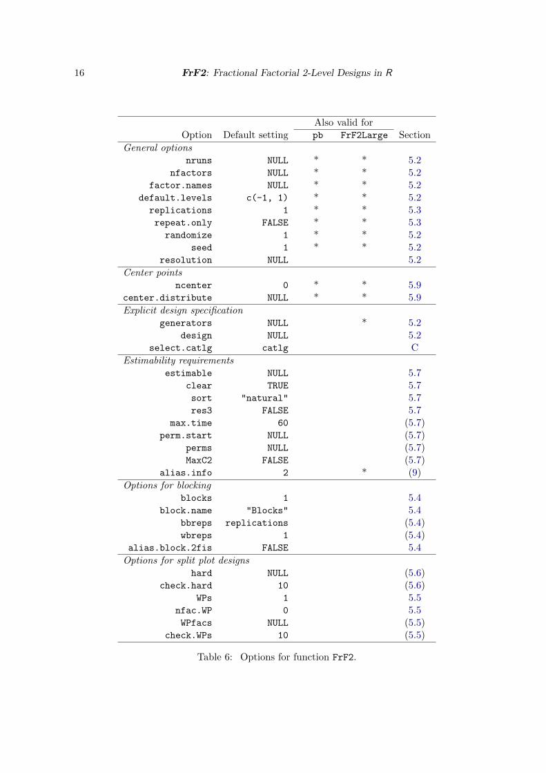
5.1. Available options
The R function FrF2 comes with many options, most of which have reasonable defaults andcan be left unspecified in most situations. Table 6 summarizes and categorizes them. Theiruse will be illustrated in the appropriate context.
Note that some specific features cannot be combined with each other – first of all, splitplotting cannot be combined with any other special feature, not even with the addition ofcenter points. Furthermore, estimability and blocking features cannot be combined with eachother.
5.2. Creating regular fractional factorial 2-level designs for simple cases
Suppose we are at the outset of planning the MI experiment; the six factors and their levelshave been tentatively fixed, and the design is to be created. Complete randomization isconsidered possible, i.e., no blocking or split plotting is necessary. All effects are consideredequally important, i.e., we want to create the MA design for the six factors; we would like tolimit the experiment to 16 runs, if a reasonable design in 16 runs exists.
16 FrF2: Fractional Factorial 2-Level Designs in R
Also valid forOption Default setting pb FrF2Large Section
General optionsnruns NULL * * 5.2
nfactors NULL * * 5.2factor.names NULL * * 5.2
default.levels c(-1, 1) * * 5.2replications 1 * * 5.3repeat.only FALSE * * 5.3randomize 1 * * 5.2
seed 1 * * 5.2resolution NULL 5.2
Center pointsncenter 0 * * 5.9
center.distribute NULL * * 5.9
Explicit design specificationgenerators NULL * 5.2
design NULL 5.2select.catlg catlg C
Estimability requirementsestimable NULL 5.7
clear TRUE 5.7sort "natural" 5.7res3 FALSE 5.7
max.time 60 (5.7)perm.start NULL (5.7)
perms NULL (5.7)MaxC2 FALSE (5.7)
alias.info 2 * (9)
Options for blockingblocks 1 5.4
block.name "Blocks" 5.4bbreps replications (5.4)wbreps 1 (5.4)
alias.block.2fis FALSE 5.4
Options for split plot designshard NULL (5.6)
check.hard 10 (5.6)WPs 1 5.5
nfac.WP 0 5.5WPfacs NULL (5.5)
check.WPs 10 (5.5)
Table 6: Options for function FrF2.
Journal of Statistical Software 17
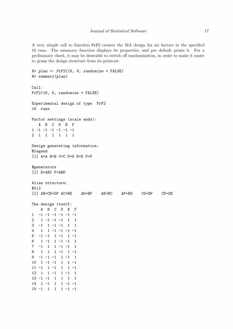
A very simple call to function FrF2 creates the MA design for six factors in the specified16 runs. The summary function displays its properties, and per default prints it. For apreliminary check, it may be desirable to switch off randomization, in order to make it easierto grasp the design structure from its printout:
R> plan <- FrF2(16, 6, randomize = FALSE)
R> summary(plan)
Call:
FrF2(16, 6, randomize = FALSE)
Experimental design of type FrF2
16 runs
Factor settings (scale ends):
A B C D E F
1 -1 -1 -1 -1 -1 -1
2 1 1 1 1 1 1
Design generating information:
$legend
[1] A=A B=B C=C D=D E=E F=F
$generators
[1] E=ABC F=ABD
Alias structure:
$fi2
[1] AB=CE=DF AC=BE AD=BF AE=BC AF=BD CD=EF CF=DE
The design itself:
A B C D E F
1 -1 -1 -1 -1 -1 -1
2 1 -1 -1 -1 1 1
3 -1 1 -1 -1 1 1
4 1 1 -1 -1 -1 -1
5 -1 -1 1 -1 1 -1
6 1 -1 1 -1 -1 1
7 -1 1 1 -1 -1 1
8 1 1 1 -1 1 -1
9 -1 -1 -1 1 -1 1
10 1 -1 -1 1 1 -1
11 -1 1 -1 1 1 -1
12 1 1 -1 1 -1 1
13 -1 -1 1 1 1 1
14 1 -1 1 1 -1 -1
15 -1 1 1 1 -1 -1
18 FrF2: Fractional Factorial 2-Level Designs in R
16 1 1 1 1 1 1
class=design, type= FrF2
The same design is also created by the following request, which leaves it to the software todetermine the smallest design in the required resolution for the given number of factors:
R> FrF2(nfactors = 6, resolution = 4, randomize = FALSE)
At the other extreme, if the user wants to specify the details, the same design can also berequested by explicit specification of its generators or by giving the design name from thecatalog catlg:
R> FrF2(design = "6-2.1", randomize = FALSE)
R> FrF2(16, gen = c("ABC", "ABD"), randomize = FALSE)
The simplest design version is convenient for quickly checking possibilities. If a design hasfinally been selected, e.g., the above design for the MI experiment, it is usually useful toadapt some options: randomization should be switched on (this is the default), and choosinga seed ensures that exactly the same randomization order can be obtained again later. Usingthe default.levels and/or factor.names options prepares easy documentation of exporteddesign files or analysis output. This is illustrated for the MI example. The first code exampleproduces the design plan with levels coded as - and + and abbreviated factor names specified:
R> plan <- FrF2(16, 6, default.levels = c("-", "+"), factor.names = c(
+ "DieOrif", "PistDiam", "Temp", "DieClean", "SMass", "BarClean"),
+ seed = 6285)
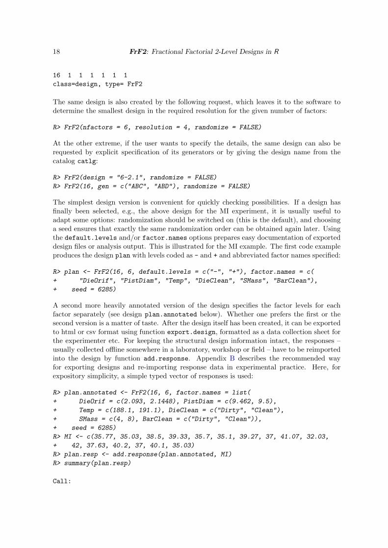
A second more heavily annotated version of the design specifies the factor levels for eachfactor separately (see design plan.annotated below). Whether one prefers the first or thesecond version is a matter of taste. After the design itself has been created, it can be exportedto html or csv format using function export.design, formatted as a data collection sheet forthe experimenter etc. For keeping the structural design information intact, the responses –usually collected offline somewhere in a laboratory, workshop or field – have to be reimportedinto the design by function add.response. Appendix B describes the recommended wayfor exporting designs and re-importing response data in experimental practice. Here, forexpository simplicity, a simple typed vector of responses is used:
R> plan.annotated <- FrF2(16, 6, factor.names = list(
+ DieOrif = c(2.093, 2.1448), PistDiam = c(9.462, 9.5),
+ Temp = c(188.1, 191.1), DieClean = c("Dirty", "Clean"),
+ SMass = c(4, 8), BarClean = c("Dirty", "Clean")),
+ seed = 6285)
R> MI <- c(35.77, 35.03, 38.5, 39.33, 35.7, 35.1, 39.27, 37, 41.07, 32.03,
+ 42, 37.63, 40.2, 37, 40.1, 35.03)
R> plan.resp <- add.response(plan.annotated, MI)
R> summary(plan.resp)
Call:
Journal of Statistical Software 19
FrF2(16, 6, factor.names = list(DieOrif = c(2.093, 2.1448), PistDiam =
c(9.462, 9.5), Temp = c(188.1, 191.1), DieClean = c("Dirty", "Clean"),
SMass = c(4, 8), BarClean = c("Dirty", "Clean")), seed = 6285)
Experimental design of type FrF2
16 runs
Factor settings (scale ends):
DieOrif PistDiam Temp DieClean SMass BarClean
1 2.0930 9.462 188.1 Dirty 4 Dirty
2 2.1448 9.500 191.1 Clean 8 Clean
Responses:
[1] MI
Design generating information:
$legend
[1] A=DieOrif B=PistDiam C=Temp D=DieClean E=SMass F=BarClean
$generators
[1] E=ABC F=ABD
Alias structure:
$fi2
[1] AB=CE=DF AC=BE AD=BF AE=BC AF=BD CD=EF CF=DE
The design itself:
DieOrif PistDiam Temp DieClean SMass BarClean MI
1 2.093 9.462 191.1 Dirty 8 Dirty 35.77
2 2.093 9.5 188.1 Clean 8 Dirty 35.03
3 2.1448 9.462 188.1 Clean 8 Dirty 38.50
4 2.1448 9.462 188.1 Dirty 8 Clean 39.33
5 2.093 9.5 188.1 Dirty 8 Clean 35.70
6 2.093 9.462 188.1 Clean 4 Clean 35.10
7 2.1448 9.5 188.1 Clean 4 Clean 39.27
8 2.093 9.5 191.1 Clean 4 Dirty 37.00
9 2.1448 9.462 191.1 Clean 4 Dirty 41.07
10 2.093 9.462 188.1 Dirty 4 Dirty 32.03
11 2.1448 9.5 191.1 Clean 8 Clean 42.00
12 2.093 9.462 191.1 Clean 8 Clean 37.63
13 2.1448 9.462 191.1 Dirty 4 Clean 40.20
14 2.1448 9.5 188.1 Dirty 4 Dirty 37.00
15 2.1448 9.5 191.1 Dirty 8 Dirty 40.10
16 2.093 9.5 191.1 Dirty 4 Clean 35.03
class=design, type= FrF2
This design will be analyzed in Section 6.
20 FrF2: Fractional Factorial 2-Level Designs in R
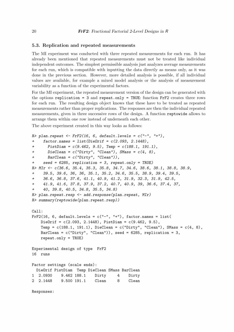
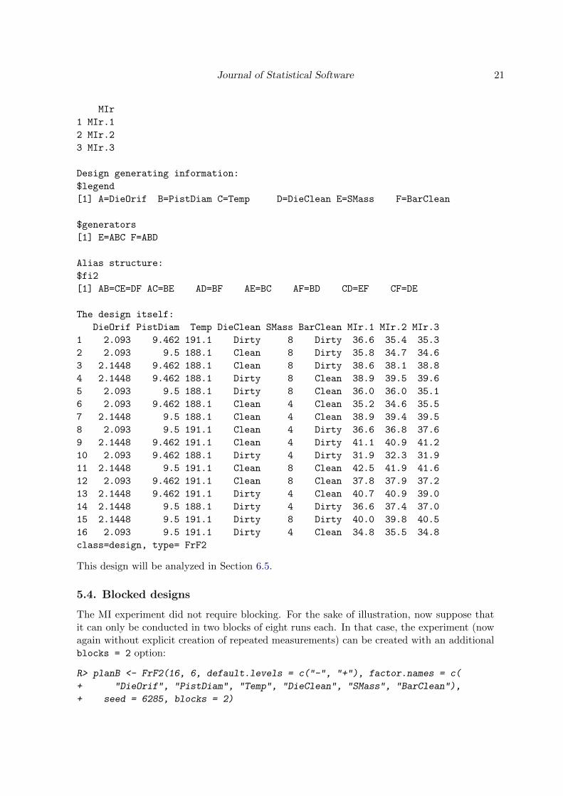
5.3. Replication and repeated measurements
The MI experiment was conducted with three repeated measurements for each run. It hasalready been mentioned that repeated measurements must not be treated like individualindependent outcomes. The simplest permissible analysis just analyzes average measurementsfor each run, which is compatible with inputting the data directly as means only, as it wasdone in the previous section. However, more detailed analysis is possible, if all individualvalues are available, for example a mixed model analysis or the analysis of measurementvariability as a function of the experimental factors.
For the MI experiment, the repeated measurement version of the design can be generated withthe options replication = 3 and repeat.only = TRUE: function FrF2 creates three rowsfor each run. The resulting design object knows that these have to be treated as repeatedmeasurements rather than proper replications. The responses are then the individual repeatedmeasurements, given in three successive rows of the design. A function reptowide allows toarrange them within one row instead of underneath each other.
The above experiment created in this way looks as follows:
R> plan.repeat <- FrF2(16, 6, default.levels = c("-", "+"),
+ factor.names = list(DieOrif = c(2.093, 2.1448),
+ PistDiam = c(9.462, 9.5), Temp = c(188.1, 191.1),
+ DieClean = c("Dirty", "Clean"), SMass = c(4, 8),
+ BarClean = c("Dirty", "Clean")),
+ seed = 6285, replication = 3, repeat.only = TRUE)
R> MIr <- c(36.6, 35.4, 35.3, 35.8, 34.7, 34.6, 38.6, 38.1, 38.8, 38.9,
+ 39.5, 39.6, 36, 36, 35.1, 35.2, 34.6, 35.5, 38.9, 39.4, 39.5,
+ 36.6, 36.8, 37.6, 41.1, 40.9, 41.2, 31.9, 32.3, 31.9, 42.5,
+ 41.9, 41.6, 37.8, 37.9, 37.2, 40.7, 40.9, 39, 36.6, 37.4, 37,
+ 40, 39.8, 40.5, 34.8, 35.5, 34.8)
R> plan.repeat.resp <- add.response(plan.repeat, MIr)
R> summary(reptowide(plan.repeat.resp))
Call:
FrF2(16, 6, default.levels = c("-", "+"), factor.names = list(
DieOrif = c(2.093, 2.1448), PistDiam = c(9.462, 9.5),
Temp = c(188.1, 191.1), DieClean = c("Dirty", "Clean"), SMass = c(4, 8),
BarClean = c("Dirty", "Clean")), seed = 6285, replication = 3,
repeat.only = TRUE)
Experimental design of type FrF2
16 runs
Factor settings (scale ends):
DieOrif PistDiam Temp DieClean SMass BarClean
1 2.0930 9.462 188.1 Dirty 4 Dirty
2 2.1448 9.500 191.1 Clean 8 Clean
Responses:
Journal of Statistical Software 21
MIr
1 MIr.1
2 MIr.2
3 MIr.3
Design generating information:
$legend
[1] A=DieOrif B=PistDiam C=Temp D=DieClean E=SMass F=BarClean
$generators
[1] E=ABC F=ABD
Alias structure:
$fi2
[1] AB=CE=DF AC=BE AD=BF AE=BC AF=BD CD=EF CF=DE
The design itself:
DieOrif PistDiam Temp DieClean SMass BarClean MIr.1 MIr.2 MIr.3
1 2.093 9.462 191.1 Dirty 8 Dirty 36.6 35.4 35.3
2 2.093 9.5 188.1 Clean 8 Dirty 35.8 34.7 34.6
3 2.1448 9.462 188.1 Clean 8 Dirty 38.6 38.1 38.8
4 2.1448 9.462 188.1 Dirty 8 Clean 38.9 39.5 39.6
5 2.093 9.5 188.1 Dirty 8 Clean 36.0 36.0 35.1
6 2.093 9.462 188.1 Clean 4 Clean 35.2 34.6 35.5
7 2.1448 9.5 188.1 Clean 4 Clean 38.9 39.4 39.5
8 2.093 9.5 191.1 Clean 4 Dirty 36.6 36.8 37.6
9 2.1448 9.462 191.1 Clean 4 Dirty 41.1 40.9 41.2
10 2.093 9.462 188.1 Dirty 4 Dirty 31.9 32.3 31.9
11 2.1448 9.5 191.1 Clean 8 Clean 42.5 41.9 41.6
12 2.093 9.462 191.1 Clean 8 Clean 37.8 37.9 37.2
13 2.1448 9.462 191.1 Dirty 4 Clean 40.7 40.9 39.0
14 2.1448 9.5 188.1 Dirty 4 Dirty 36.6 37.4 37.0
15 2.1448 9.5 191.1 Dirty 8 Dirty 40.0 39.8 40.5
16 2.093 9.5 191.1 Dirty 4 Clean 34.8 35.5 34.8
class=design, type= FrF2
This design will be analyzed in Section 6.5.
5.4. Blocked designs
The MI experiment did not require blocking. For the sake of illustration, now suppose thatit can only be conducted in two blocks of eight runs each. In that case, the experiment (nowagain without explicit creation of repeated measurements) can be created with an additionalblocks = 2 option:
R> planB <- FrF2(16, 6, default.levels = c("-", "+"), factor.names = c(
+ "DieOrif", "PistDiam", "Temp", "DieClean", "SMass", "BarClean"),
+ seed = 6285, blocks = 2)
22 FrF2: Fractional Factorial 2-Level Designs in R
R> summary(planB)
Call:
FrF2(16, 6, default.levels = c("-", "+"), factor.names = c("DieOrif",
"PistDiam", "Temp", "DieClean", "SMass", "BarClean"), seed = 6285,
blocks = 2)
Experimental design of type FrF2.blocked
16 runs
blocked design with 2 blocks of size 8
Factor settings (scale ends):
DieOrif PistDiam Temp DieClean SMass BarClean
1 - - - - - -
2 + + + + + +
Design generating information:
$legend
[1] A=DieOrif B=PistDiam C=Temp D=DieClean E=SMass F=BarClean
$`generators for design itself`
[1] E=ABC F=ABD
$`block generators`
[1] ACD
Alias structure:
$fi2
[1] AB=CE=DF AC=BE AD=BF AE=BC AF=BD CD=EF CF=DE
Aliased with block main effects:
[1] none
The design itself:
run.no run.no.std.rp Blocks DieOrif PistDiam Temp DieClean SMass BarClean
1 1 5.1.3 1 - + - - + +
2 2 10.1.5 1 + - - + + -
3 3 8.1.4 1 - + + + - -
4 4 1.1.1 1 - - - - - -
5 5 14.1.7 1 + + - + - +
6 6 15.1.8 1 + + + - + -
7 7 11.1.6 1 + - + - - +
8 8 4.1.2 1 - - + + + +
run.no run.no.std.rp Blocks DieOrif PistDiam Temp DieClean SMass BarClean
9 9 6.2.3 2 - + - + + -
10 10 2.2.1 2 - - - + - +
11 11 9.2.5 2 + - - - + +
Journal of Statistical Software 23
12 12 3.2.2 2 - - + - + -
13 13 12.2.6 2 + - + + - -
14 14 7.2.4 2 - + + - - +
15 15 16.2.8 2 + + + + + +
16 16 13.2.7 2 + + - - - -
class=design, type= FrF2.blocked
NOTE: columns run.no and run.no.std.rp are annotation, not part of the data
frame
The output above is annotated with block information from the run.order attribute of thedesign. The column run.no.std.rp contains the original run number in the non-randomizeddesign in Yates order, the block number and the original position of the run within that block.The rp in run.no.std.rp stands for replication information; if there are replications and/orrepeated measurements, this will also be reflected in further components of run.no.std.rp.Note that, for blocked and split plot designs, the run number in standard order refers to therun order with the first base factor changing slowest, which was also mentioned in Section 3.1,as that this is the order from which blocked or split plot designs are created. As an aside,also note that the run number in standard order in case of designs with estimable 2fis (seeSection 5.7) or split plotting (see Section 5.5) can be based on an unexpected selection andordering of base factors (this is documented in the help file for function FrF2).
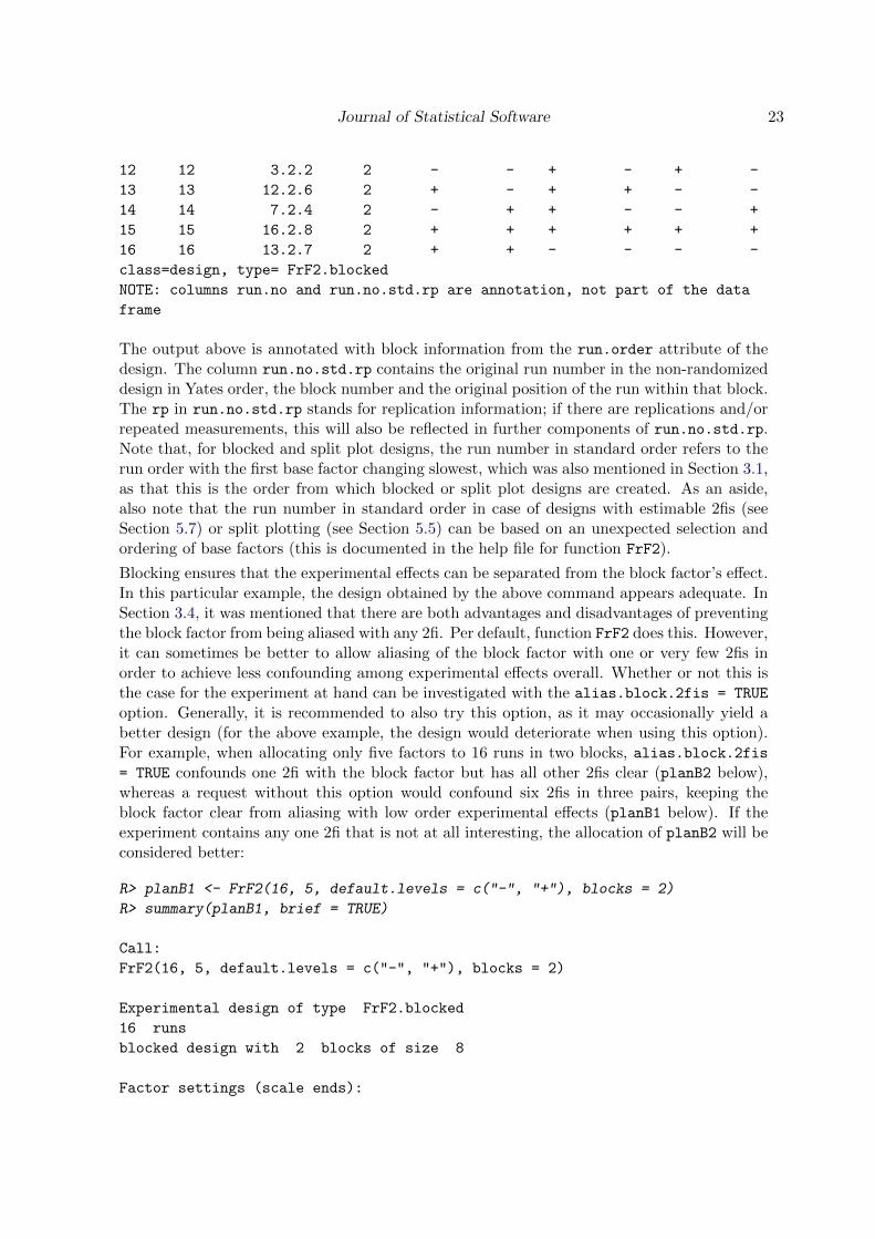
Blocking ensures that the experimental effects can be separated from the block factor’s effect.In this particular example, the design obtained by the above command appears adequate. InSection 3.4, it was mentioned that there are both advantages and disadvantages of preventingthe block factor from being aliased with any 2fi. Per default, function FrF2 does this. However,it can sometimes be better to allow aliasing of the block factor with one or very few 2fis inorder to achieve less confounding among experimental effects overall. Whether or not this isthe case for the experiment at hand can be investigated with the alias.block.2fis = TRUE
option. Generally, it is recommended to also try this option, as it may occasionally yield abetter design (for the above example, the design would deteriorate when using this option).For example, when allocating only five factors to 16 runs in two blocks, alias.block.2fis= TRUE confounds one 2fi with the block factor but has all other 2fis clear (planB2 below),whereas a request without this option would confound six 2fis in three pairs, keeping theblock factor clear from aliasing with low order experimental effects (planB1 below). If theexperiment contains any one 2fi that is not at all interesting, the allocation of planB2 will beconsidered better:
R> planB1 <- FrF2(16, 5, default.levels = c("-", "+"), blocks = 2)
R> summary(planB1, brief = TRUE)
Call:
FrF2(16, 5, default.levels = c("-", "+"), blocks = 2)
Experimental design of type FrF2.blocked
16 runs
blocked design with 2 blocks of size 8
Factor settings (scale ends):
24 FrF2: Fractional Factorial 2-Level Designs in R
A B C D E
1 - - - - -
2 + + + + +
Design generating information:
$legend
[1] A=A B=B C=C D=D E=E
$`generators for design itself`
[1] E=ABC
$`block generators`
[1] ABD
Alias structure:
$fi2
[1] AB=CE AC=BE AE=BC
Aliased with block main effects:
[1] none
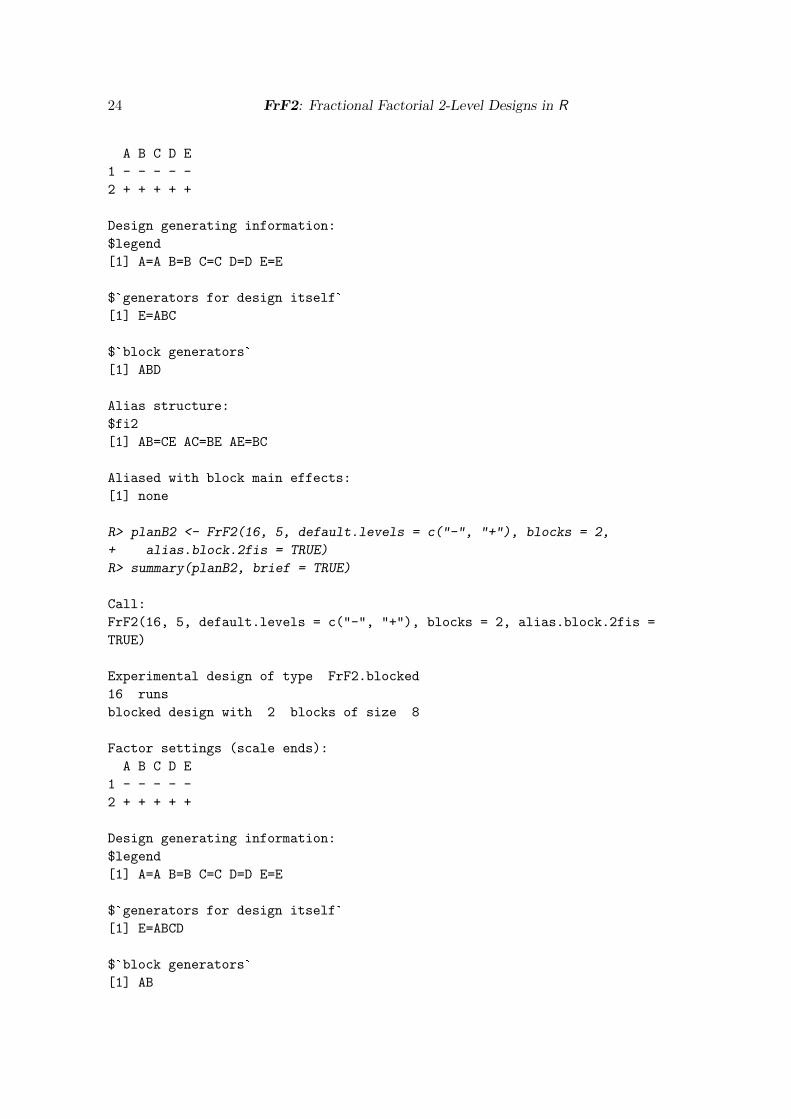
R> planB2 <- FrF2(16, 5, default.levels = c("-", "+"), blocks = 2,
+ alias.block.2fis = TRUE)
R> summary(planB2, brief = TRUE)
Call:
FrF2(16, 5, default.levels = c("-", "+"), blocks = 2, alias.block.2fis =
TRUE)
Experimental design of type FrF2.blocked
16 runs
blocked design with 2 blocks of size 8
Factor settings (scale ends):
A B C D E
1 - - - - -
2 + + + + +
Design generating information:
$legend
[1] A=A B=B C=C D=D E=E
$`generators for design itself`
[1] E=ABCD
$`block generators`
[1] AB
Journal of Statistical Software 25
no aliasing of main effects or 2fis among experimental factors
Aliased with block main effects:
[1] AB
Alternatively to the automatic generation, it is also possible to specify the generators for theexperimental factors themselves (option generators) and the generators for the block factor(give to option blocks instead of number of blocks). For example, design planB2 for the fivefactors can also be created by the command
R> FrF2(16, 5, default.levels = c("-", "+"), generators = "ABCD",
+ blocks = "AB")
With explicit specification of block generators, the user is responsible for their alias behavior,and option alias.block.2fis is not needed. The online help for function FrF2 mentionsfurther possibilities of specifying option blocks, which are not covered in this article.
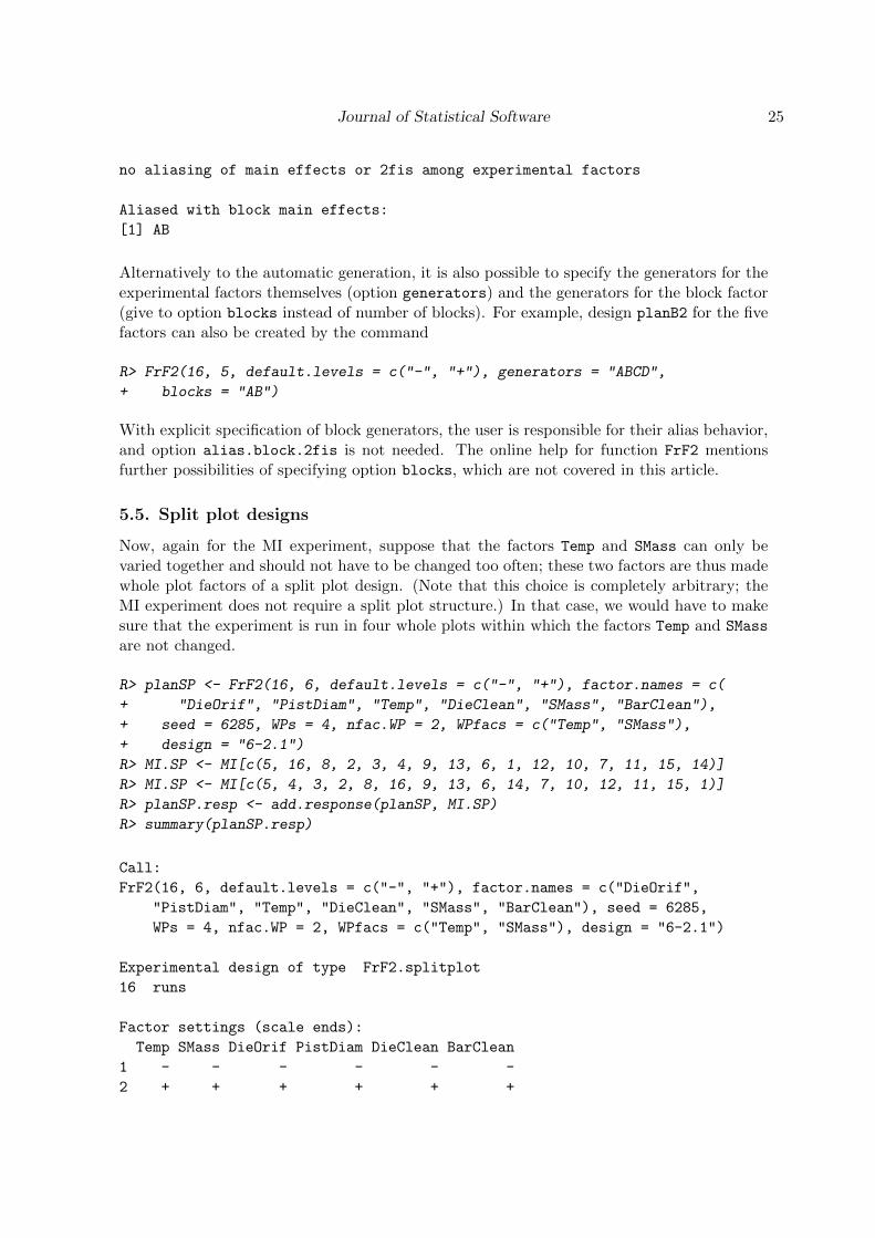
5.5. Split plot designs
Now, again for the MI experiment, suppose that the factors Temp and SMass can only bevaried together and should not have to be changed too often; these two factors are thus madewhole plot factors of a split plot design. (Note that this choice is completely arbitrary; theMI experiment does not require a split plot structure.) In that case, we would have to makesure that the experiment is run in four whole plots within which the factors Temp and SMass
are not changed.
R> planSP <- FrF2(16, 6, default.levels = c("-", "+"), factor.names = c(
+ "DieOrif", "PistDiam", "Temp", "DieClean", "SMass", "BarClean"),
+ seed = 6285, WPs = 4, nfac.WP = 2, WPfacs = c("Temp", "SMass"),
+ design = "6-2.1")
R> MI.SP <- MI[c(5, 16, 8, 2, 3, 4, 9, 13, 6, 1, 12, 10, 7, 11, 15, 14)]
R> MI.SP <- MI[c(5, 4, 3, 2, 8, 16, 9, 13, 6, 14, 7, 10, 12, 11, 15, 1)]
R> planSP.resp <- add.response(planSP, MI.SP)
R> summary(planSP.resp)
Call:
FrF2(16, 6, default.levels = c("-", "+"), factor.names = c("DieOrif",
"PistDiam", "Temp", "DieClean", "SMass", "BarClean"), seed = 6285,
WPs = 4, nfac.WP = 2, WPfacs = c("Temp", "SMass"), design = "6-2.1")
Experimental design of type FrF2.splitplot
16 runs
Factor settings (scale ends):
Temp SMass DieOrif PistDiam DieClean BarClean
1 - - - - - -
2 + + + + + +
26 FrF2: Fractional Factorial 2-Level Designs in R
Responses:
[1] MI.SP
Design generating information:
$legend
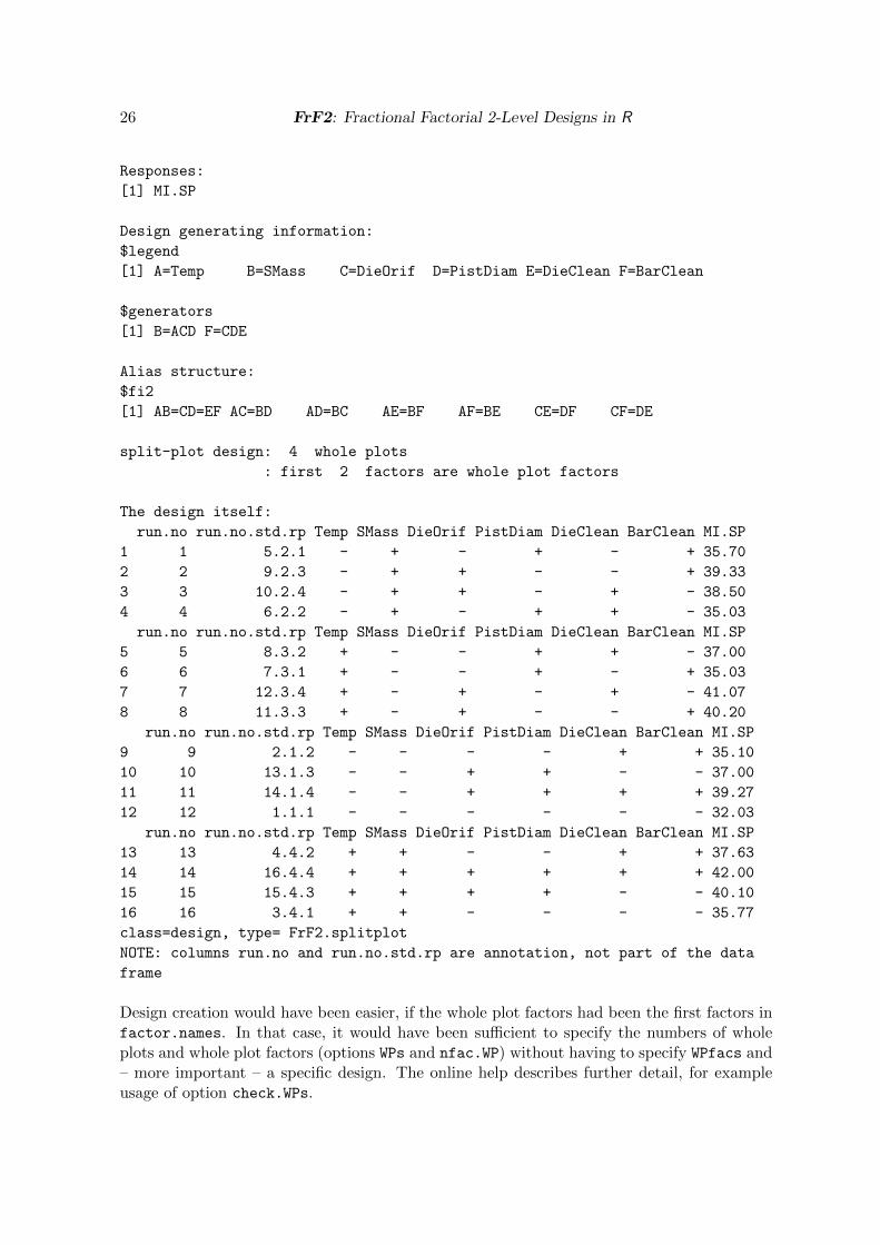
[1] A=Temp B=SMass C=DieOrif D=PistDiam E=DieClean F=BarClean
$generators
[1] B=ACD F=CDE
Alias structure:
$fi2
[1] AB=CD=EF AC=BD AD=BC AE=BF AF=BE CE=DF CF=DE
split-plot design: 4 whole plots
: first 2 factors are whole plot factors
The design itself:
run.no run.no.std.rp Temp SMass DieOrif PistDiam DieClean BarClean MI.SP
1 1 5.2.1 - + - + - + 35.70
2 2 9.2.3 - + + - - + 39.33
3 3 10.2.4 - + + - + - 38.50
4 4 6.2.2 - + - + + - 35.03
run.no run.no.std.rp Temp SMass DieOrif PistDiam DieClean BarClean MI.SP
5 5 8.3.2 + - - + + - 37.00
6 6 7.3.1 + - - + - + 35.03
7 7 12.3.4 + - + - + - 41.07
8 8 11.3.3 + - + - - + 40.20
run.no run.no.std.rp Temp SMass DieOrif PistDiam DieClean BarClean MI.SP
9 9 2.1.2 - - - - + + 35.10
10 10 13.1.3 - - + + - - 37.00
11 11 14.1.4 - - + + + + 39.27
12 12 1.1.1 - - - - - - 32.03
run.no run.no.std.rp Temp SMass DieOrif PistDiam DieClean BarClean MI.SP
13 13 4.4.2 + + - - + + 37.63
14 14 16.4.4 + + + + + + 42.00
15 15 15.4.3 + + + + - - 40.10
16 16 3.4.1 + + - - - - 35.77
class=design, type= FrF2.splitplot
NOTE: columns run.no and run.no.std.rp are annotation, not part of the data
frame
Design creation would have been easier, if the whole plot factors had been the first factors infactor.names. In that case, it would have been sufficient to specify the numbers of wholeplots and whole plot factors (options WPs and nfac.WP) without having to specify WPfacs and– more important – a specific design. The online help describes further detail, for exampleusage of option check.WPs.
Journal of Statistical Software 27
In the creation of the split plot experiment above, it had to be made sure that the experimentwas created such that the response values from the published MI experiment can be used fordemonstrating analysis features for split plot designs later on, as response values are availablefor 16 level combinations of the 64 possible ones only. The 16 response values (averages usedagain) had to be reordered, as the split plot structure implies a randomized ordering differentfrom the previous one. The design planSP.resp will be used for demonstrating the onlyanalysis feature for split plot designs in Section 6.4.
5.6. Hard to change factors
The previous section discussed split plotting. Split plotting can also be used for accomodatinghard to change factors, by making these the whole plot factors. Sometimes, researcherssee the need to enforce even fewer changes than obtainable from such a split plot designwith randomized whole plots. This can be achieved in function FrF2, using option hard forspecifying the number of hard to change factors (these have to be the first factors specified);the function uses the slow-changing matrix given in Cheng et al. (1998). This option createsa split plot design with non-randomized and very systematic order of whole plots; runs withinwhole plots are randomized, like always. The resulting design is a multilevel split plot design:the first hard to change factor changes most slowly, the second one second most slowly etc.As long as
� the order of the runs is not influential,
� and the variability from changing hard-to-change factors is close to negligible relativeto measurement variability and variability from changing easy-to-change factors,
a pragmatic researcher may consider this type of procedure as preferrable to not being ableto conduct the experiment. Therefore, the package offers this type of design. For analysis,the package treats such a design as a split plot design, although its whole plot order is notrandomized. It must be emphasized that the user is responsible for assessing whether theapproach can be responsibly used. Whenever feasible, a proper split plot design with the hardto change factors as whole plot factors (and resetting their levels between whole plots even ifthere is no level change between adjacent whole plots!) should be used instead!
5.7. Estimability of two-factor interactions in package FrF2
The general option resolution is adequate whenever users simply want to treat all effectsof the same order in the same way. Mainly for resolution IV designs, it is not uncommon toconsider some 2fis to be more important than others, as was discussed in Section 3.3. For thissituation, option estimable selects these more important 2fis (the requirement set), optionclear governs whether or not a clear design is requested, and option res3 allows the user todowngrade from the natural requirement of resolution IV to resolution III only. The otherestimability options from Table 6 handle technicalities, more or less. Note that the generaloption resolution cannot be specified together with the estimable option.
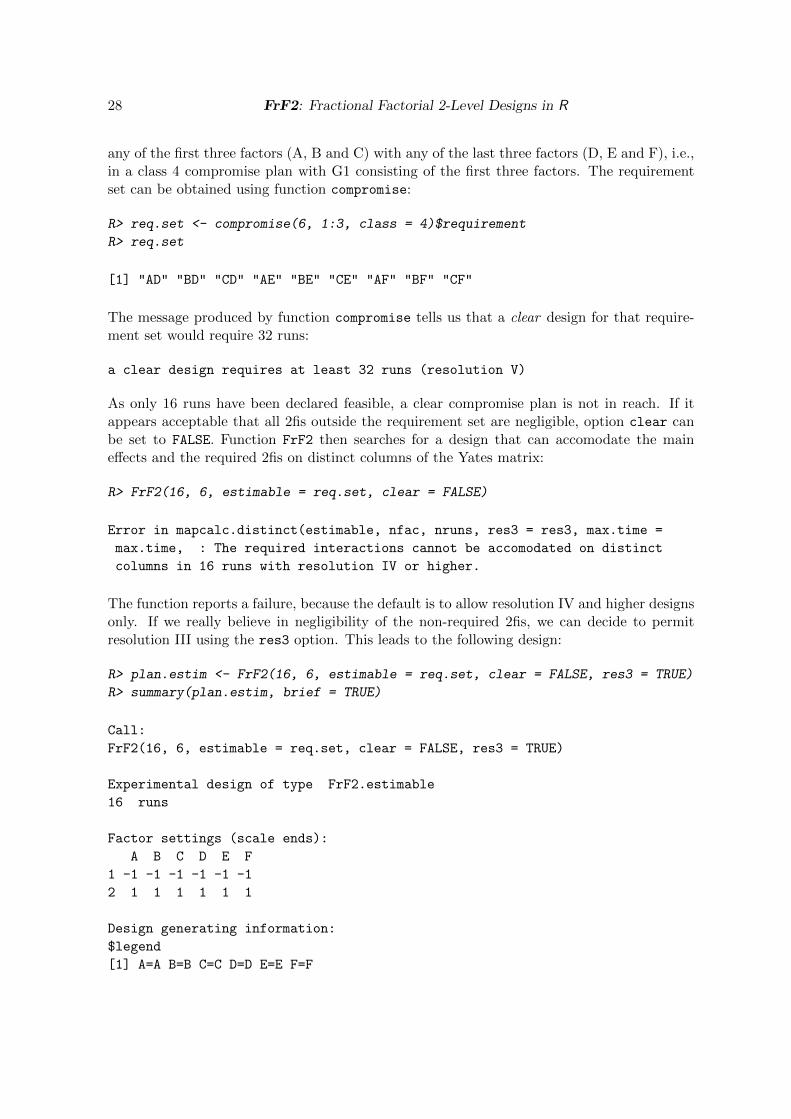
Distinct designs
For demonstrating estimability features, let us now consider the MI experiment, assumingthat we can afford 16 runs only and that we are interested in the main effects and the 2fis of
28 FrF2: Fractional Factorial 2-Level Designs in R
any of the first three factors (A, B and C) with any of the last three factors (D, E and F), i.e.,in a class 4 compromise plan with G1 consisting of the first three factors. The requirementset can be obtained using function compromise:
R> req.set <- compromise(6, 1:3, class = 4)$requirement
R> req.set
[1] "AD" "BD" "CD" "AE" "BE" "CE" "AF" "BF" "CF"
The message produced by function compromise tells us that a clear design for that require-ment set would require 32 runs:
a clear design requires at least 32 runs (resolution V)
As only 16 runs have been declared feasible, a clear compromise plan is not in reach. If itappears acceptable that all 2fis outside the requirement set are negligible, option clear canbe set to FALSE. Function FrF2 then searches for a design that can accomodate the maineffects and the required 2fis on distinct columns of the Yates matrix:
R> FrF2(16, 6, estimable = req.set, clear = FALSE)
Error in mapcalc.distinct(estimable, nfac, nruns, res3 = res3, max.time =
max.time, : The required interactions cannot be accomodated on distinct
columns in 16 runs with resolution IV or higher.
The function reports a failure, because the default is to allow resolution IV and higher designsonly. If we really believe in negligibility of the non-required 2fis, we can decide to permitresolution III using the res3 option. This leads to the following design:
R> plan.estim <- FrF2(16, 6, estimable = req.set, clear = FALSE, res3 = TRUE)
R> summary(plan.estim, brief = TRUE)
Call:
FrF2(16, 6, estimable = req.set, clear = FALSE, res3 = TRUE)
Experimental design of type FrF2.estimable
16 runs
Factor settings (scale ends):
A B C D E F
1 -1 -1 -1 -1 -1 -1
2 1 1 1 1 1 1
Design generating information:
$legend
[1] A=A B=B C=C D=D E=E F=F
Journal of Statistical Software 29
$generators
[1] C=AB F=ADE
Alias structure:
$main
[1] A=BC B=AC C=AB
$fi2
[1] AD=EF AE=DF AF=DE
The output shows that the design plan.estim confounds main effects of factors A, B and Cwith the 2fi of the respective other two factors. As these 2fis have been assumed negligible, thisdesign is acceptable under the “distinct” approach. For readers interested in the generation ofthe array, the map entry of the design.info attribute of the design shows that it was obtainedby using the second best design for 6 factors in 16 runs, and by pulling the 5th design factorto the third position in order to make the design match the required structure (i.e., A = 1, B= 2, C = 5, D = 3, E = 4, F = 6):
R> design.info(plan.estim)$map
$`6-2.2`
[1] 1 2 5 3 4 6
Clear designs
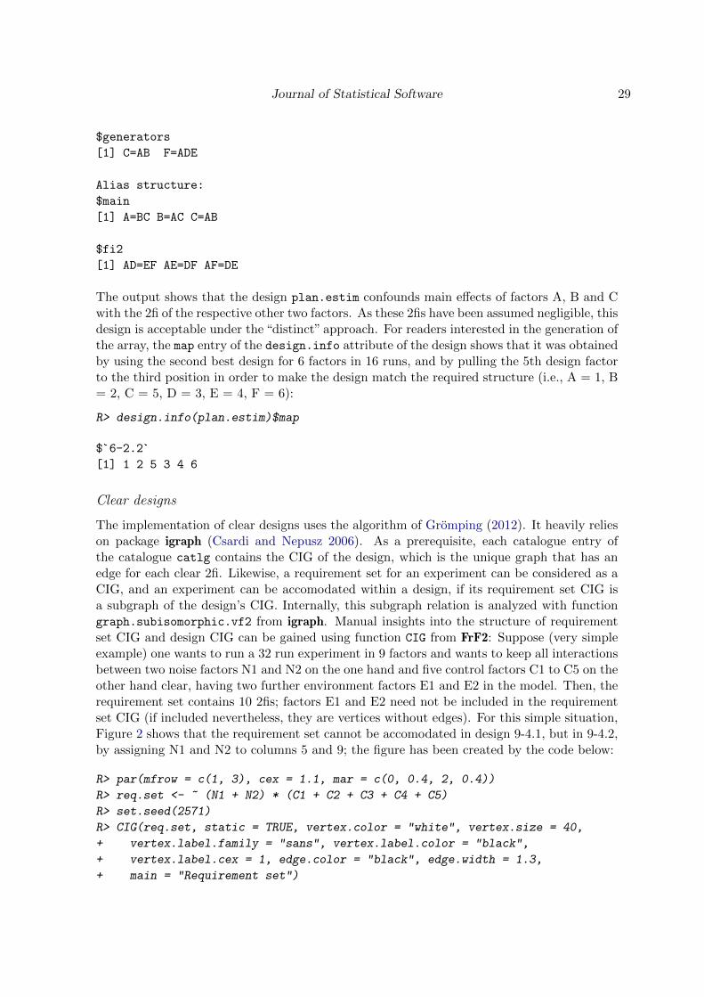
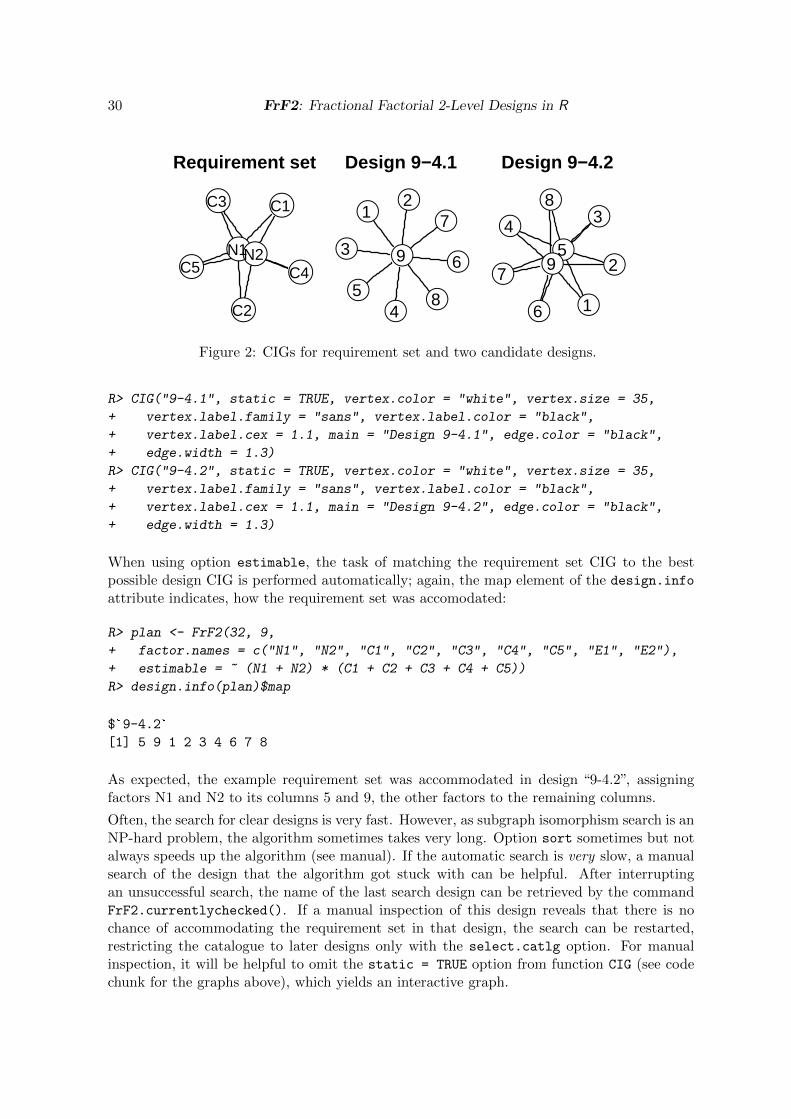
The implementation of clear designs uses the algorithm of Gromping (2012). It heavily relieson package igraph (Csardi and Nepusz 2006). As a prerequisite, each catalogue entry ofthe catalogue catlg contains the CIG of the design, which is the unique graph that has anedge for each clear 2fi. Likewise, a requirement set for an experiment can be considered as aCIG, and an experiment can be accomodated within a design, if its requirement set CIG isa subgraph of the design’s CIG. Internally, this subgraph relation is analyzed with functiongraph.subisomorphic.vf2 from igraph. Manual insights into the structure of requirementset CIG and design CIG can be gained using function CIG from FrF2: Suppose (very simpleexample) one wants to run a 32 run experiment in 9 factors and wants to keep all interactionsbetween two noise factors N1 and N2 on the one hand and five control factors C1 to C5 on theother hand clear, having two further environment factors E1 and E2 in the model. Then, therequirement set contains 10 2fis; factors E1 and E2 need not be included in the requirementset CIG (if included nevertheless, they are vertices without edges). For this simple situation,Figure 2 shows that the requirement set cannot be accomodated in design 9-4.1, but in 9-4.2,by assigning N1 and N2 to columns 5 and 9; the figure has been created by the code below:
R> par(mfrow = c(1, 3), cex = 1.1, mar = c(0, 0.4, 2, 0.4))
R> req.set <- ~ (N1 + N2) * (C1 + C2 + C3 + C4 + C5)
R> set.seed(2571)
R> CIG(req.set, static = TRUE, vertex.color = "white", vertex.size = 40,
+ vertex.label.family = "sans", vertex.label.color = "black",
+ vertex.label.cex = 1, edge.color = "black", edge.width = 1.3,
+ main = "Requirement set")
30 FrF2: Fractional Factorial 2-Level Designs in R
Requirement set
●●
●
●
●
●●N1N2
C1
C2
C3
C4C5
Design 9−4.1
● ●
●
●●
●
●
●
●
12
3
45
6
7
8
9
Design 9−4.2
●
●
●●●
●
●
●
●
1
2
34
5
6
7
8
9
Figure 2: CIGs for requirement set and two candidate designs.
R> CIG("9-4.1", static = TRUE, vertex.color = "white", vertex.size = 35,
+ vertex.label.family = "sans", vertex.label.color = "black",
+ vertex.label.cex = 1.1, main = "Design 9-4.1", edge.color = "black",
+ edge.width = 1.3)
R> CIG("9-4.2", static = TRUE, vertex.color = "white", vertex.size = 35,
+ vertex.label.family = "sans", vertex.label.color = "black",
+ vertex.label.cex = 1.1, main = "Design 9-4.2", edge.color = "black",
+ edge.width = 1.3)
When using option estimable, the task of matching the requirement set CIG to the bestpossible design CIG is performed automatically; again, the map element of the design.info
attribute indicates, how the requirement set was accomodated:
R> plan <- FrF2(32, 9,
+ factor.names = c("N1", "N2", "C1", "C2", "C3", "C4", "C5", "E1", "E2"),
+ estimable = ~ (N1 + N2) * (C1 + C2 + C3 + C4 + C5))
R> design.info(plan)$map
$`9-4.2`
[1] 5 9 1 2 3 4 6 7 8
As expected, the example requirement set was accommodated in design “9-4.2”, assigningfactors N1 and N2 to its columns 5 and 9, the other factors to the remaining columns.
Often, the search for clear designs is very fast. However, as subgraph isomorphism search is anNP-hard problem, the algorithm sometimes takes very long. Option sort sometimes but notalways speeds up the algorithm (see manual). If the automatic search is very slow, a manualsearch of the design that the algorithm got stuck with can be helpful. After interruptingan unsuccessful search, the name of the last search design can be retrieved by the commandFrF2.currentlychecked(). If a manual inspection of this design reveals that there is nochance of accommodating the requirement set in that design, the search can be restarted,restricting the catalogue to later designs only with the select.catlg option. For manualinspection, it will be helpful to omit the static = TRUE option from function CIG (see codechunk for the graphs above), which yields an interactive graph.
Journal of Statistical Software 31
5.8. Large designs
Function FrF2 is limited to designs with up to 4096 runs, regardless of the way a design isspecified. Larger fractional factorial 2-level designs can be created with function FrF2Large.The latter function is more limited than FrF2 in terms of design structures (no blocking, nosplit plot designs, no estimability requirements). The available options are those asteriskedin Table 6. Function FrF2Large implements automatic design creation with the method bySanchez and Sanchez (2005) that was introduced in Section 3.2. Alternatively, users canmanually generate a design by specifying the generators (with slightly more restrictive entriesthan in function FrF2). Attempts to use this function for designs with up to 4096 runs returnan error.
5.9. Randomization, replication and center points
Center points
Regular fractional factorial 2-level designs with quantitative factors are often used as thestarting point for response surface investigations. For these, it can be quite useful to usesome center points in the design. Center points can also be useful for checking for curvaturein non-regular fractional factorial 2-level designs. Center points can be requested with optionncenter of functions FrF2, FrF2Large and pb. Note that their position in the design is notrandomized, but can be controlled via option center.distribute. Per default, center pointsare placed at the beginning, in the middle and at the end of the design (i.e., distributed overthree points). It is also possible to augment a design with center points after its creationusing function add.center.
Note that the center points functionality does not work simultaneously with a split plotstructure or specification of hard to change factors. The reason is that it is usually not agood idea to have a separate whole plot that consists of center points only, and that it is notobvious how to handle center points in a standard way in split plot designs.
Randomization and replication
Design generating functions generally block the randomization of proper replications on time,i.e., they generate a randomized sequence of all first replicates, then a randomized sequenceof all second replicates, and so forth (run FrF2(8, 4, replications = 3) to see what thismeans). As the user has not a-priori specified time as a block factor, this is a mere precautionagainst surprises from time effects that are not unheard of; if such a time trend is found, ananalysis including a replication block factor can partially account for it. However, since theuser did not ask for blocking on time in the first place, the replicated design does not containa block column, and its default analysis does not include a block factor.
If desired, the block factor that reflects the replication blocking on time can be retrieved usingfunction getblock; this function will also provide separate factors for the other randomizationrestrictions. Users can use these factors in a custom analysis with R function lm or advancedanalysis functions from packages.
Users who dislike the fact that replications are blocked on time or that center points aresystematically placed can apply the function rerandomize.design to the design; this func-tion does not randomize the replications in blocks and does randomize the position of center
32 FrF2: Fractional Factorial 2-Level Designs in R
points, and it also randomizes the position of blocks; in the default randomization, blockorder is fixed, and it is assumed that users randomize their units to the blocks. Of course,rerandomize.design keeps a block or split plot structure intact and keeps repeated mea-surements together. Users who decide to use this function have to make sure to add centerpoints directly with design creation, as subsequent adding of center points is not possible fora re-randomized design.
6. Simple analysis tools
Simple analysis tools for regular fractional factorial 2-level designs have been discussed inSection 3.1. Their R implementation is presented here, using the MI experiment. As aprerequisite of any useful interpretation, awareness of the alias structure – obtainable fromthe summary function – is necessary.
6.1. Main effects plots
A very simple analysis visualizes the response means for the different factor levels: the maineffects plot. Two versions of main effects plots are available, and which one to use is purelya matter of taste:
R> plot(plan.resp, cex = 1.2, cex.lab = 1.2, cex.axis = 1.2,
+ main = "Main effects plot for MI", cex.main = 2)
R> MEPlot(plan.resp, abbrev = 5, cex.xax = 1.6, cex.main = 2)
The main effects plot for the MI experiment (both graphs in Figure 3) shows the differencesbetween factor levels. Clearly, controlling the die orifice diameter has the largest effect, witha difference of about 4.3 between its levels. Temperature follows suit, with a difference ofabout 2. The relevance of the effect sizes can usually be decided by the experimenter’s gutfeel, while the significance must be decided by statistical methods (see Sections 6.3 and 6.4).
In resolution III designs, the user should be aware of aliased 2fis which can mask or inflate amain effect. This is not an issue in the resolution IV MI experiment.
6.2. Interaction plots
For resolution IV or higher regular fractional factorial 2-level designs, it makes sense to lookat interaction plots. Function IAPlot with its method for class design objects can be usedfor that purpose. The graphs in Figure 4 have been created with the following code:
R> IAPlot(plan.resp, abbrev = 5, show.alias = TRUE, lwd = 2, cex = 2,
+ cex.xax = 1.2, cex.lab = 1.5)
R> IAPlot(plan.resp, abbrev = 5, select = 3:6, lwd = 2, cex = 2,
+ cex.xax = 1.2, cex.lab = 1.5)
The show.alias = TRUE option marks aliased interactions with the same number in order toindicate that these can only be estimated together in one sum (see top graph in Figure 4); thisis very helpful for avoiding over-interpretation. For example, the summary of the design inSection 5.2 showed that the interaction between temperature and barrel cleanliness is aliased
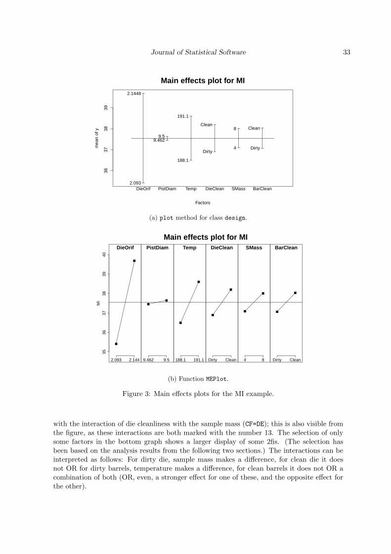
Journal of Statistical Software 33
3637
3839
Main effects plot for MI
Factors
mea
n of
y
2.093
2.1448
9.4629.5
188.1
191.1
Dirty
Clean
4
8
Dirty
Clean
DieOrif PistDiam Temp DieClean SMass BarClean
(a) plot method for class design.
DieOrif
MI
2.093 2.144
3536
3738
3940
PistDiam
9.462 9.5
Temp
188.1 191.1
DieClean
Dirty Clean
SMass
4 8
BarClean
Dirty Clean
Main effects plot for MI
(b) Function MEPlot.
Figure 3: Main effects plots for the MI example.
with the interaction of die cleanliness with the sample mass (CF=DE); this is also visible fromthe figure, as these interactions are both marked with the number 13. The selection of onlysome factors in the bottom graph shows a larger display of some 2fis. (The selection hasbeen based on the analysis results from the following two sections.) The interactions can beinterpreted as follows: For dirty die, sample mass makes a difference, for clean die it doesnot OR for dirty barrels, temperature makes a difference, for clean barrels it does not OR acombination of both (OR, even, a stronger effect for one of these, and the opposite effect forthe other).
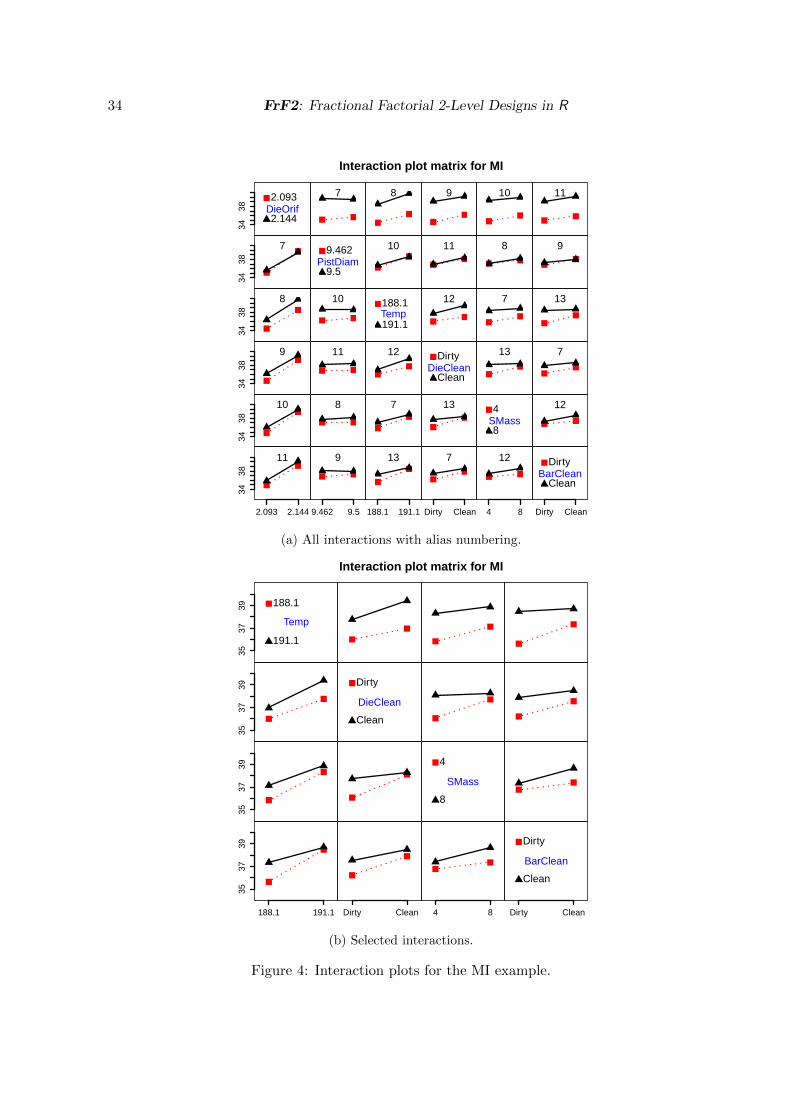
34 FrF2: Fractional Factorial 2-Level Designs in R
MI
2.093
2.144DieOrif
3438
PistDiam
MI
3438
7
Temp
MI
3438
8
DieClean
MI
3438
9
SMass
MI
3438
10
BarClean
MI
3438
2.093 2.144
11
DieOrif
MI
7
MI
9.462
9.5PistDiam
Temp
MI
10
DieClean
MI
11
SMass
MI
8
BarClean
MI
9.462 9.5
9
DieOrif
MI
8
PistDiam
MI
10
MI
188.1
191.1Temp
DieClean
MI
12
SMass
MI
7
BarClean
MI
188.1 191.1
13
DieOrif
MI
9
PistDiam
MI
11
Temp
MI
12
MI
Dirty
CleanDieClean
SMass
MI
13
BarClean
MI
Dirty Clean
7
DieOrif
MI
10
PistDiam
MI
8
Temp
MI
7
DieClean
MI
13
MI
4
8SMass
BarClean
MI
4 8
12
DieOrif
MI
11
PistDiam
MI
9
Temp
MI
13
DieClean
MI
7
SMass
MI
12
MI
Dirty
CleanBarClean
Dirty Clean
Interaction plot matrix for MI
(a) All interactions with alias numbering.
MI
188.1
191.1
Temp
3537
39
DieClean
MI
3537
39
SMass
MI
3537
39
BarClean
MI
3537
39
188.1 191.1
Temp
MI
MI
Dirty
Clean
DieClean
SMass
MI
BarClean
MI
Dirty Clean
Temp
MI
DieClean
MI
MI
4
8
SMass
BarClean
MI
4 8
Temp
MI
DieClean
MI
SMass
MI
MI
Dirty
Clean
BarClean
Dirty Clean
Interaction plot matrix for MI
(b) Selected interactions.
Figure 4: Interaction plots for the MI example.
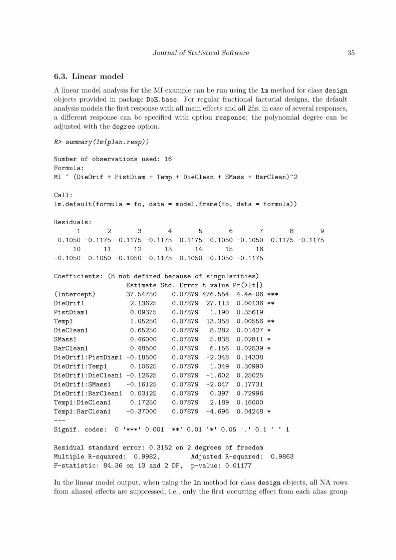
Journal of Statistical Software 35
6.3. Linear model
A linear model analysis for the MI example can be run using the lm method for class designobjects provided in package DoE.base. For regular fractional factorial designs, the defaultanalysis models the first response with all main effects and all 2fis; in case of several responses,a different response can be specified with option response; the polynomial degree can beadjusted with the degree option.
R> summary(lm(plan.resp))
Number of observations used: 16
Formula:
MI ~ (DieOrif + PistDiam + Temp + DieClean + SMass + BarClean)^2
Call:
lm.default(formula = fo, data = model.frame(fo, data = formula))
Residuals:
1 2 3 4 5 6 7 8 9
0.1050 -0.1175 0.1175 -0.1175 0.1175 0.1050 -0.1050 0.1175 -0.1175
10 11 12 13 14 15 16
-0.1050 0.1050 -0.1050 0.1175 0.1050 -0.1050 -0.1175
Coefficients: (8 not defined because of singularities)
Estimate Std. Error t value Pr(>|t|)
(Intercept) 37.54750 0.07879 476.554 4.4e-06 ***
DieOrif1 2.13625 0.07879 27.113 0.00136 **
PistDiam1 0.09375 0.07879 1.190 0.35619
Temp1 1.05250 0.07879 13.358 0.00556 **
DieClean1 0.65250 0.07879 8.282 0.01427 *
SMass1 0.46000 0.07879 5.838 0.02811 *
BarClean1 0.48500 0.07879 6.156 0.02539 *
DieOrif1:PistDiam1 -0.18500 0.07879 -2.348 0.14338
DieOrif1:Temp1 0.10625 0.07879 1.349 0.30990
DieOrif1:DieClean1 -0.12625 0.07879 -1.602 0.25025
DieOrif1:SMass1 -0.16125 0.07879 -2.047 0.17731
DieOrif1:BarClean1 0.03125 0.07879 0.397 0.72996
Temp1:DieClean1 0.17250 0.07879 2.189 0.16000
Temp1:BarClean1 -0.37000 0.07879 -4.696 0.04248 *
---
Signif. codes: 0 '***' 0.001 '**' 0.01 '*' 0.05 '.' 0.1 ' ' 1
Residual standard error: 0.3152 on 2 degrees of freedom
Multiple R-squared: 0.9982, Adjusted R-squared: 0.9863
F-statistic: 84.36 on 13 and 2 DF, p-value: 0.01177
In the linear model output, when using the lm method for class design objects, all NA rowsfrom aliased effects are suppressed, i.e., only the first occurring effect from each alias group
36 FrF2: Fractional Factorial 2-Level Designs in R
is included. For example, the MI experiment has six main effects and 15 2fis; the outputshows only seven 2fis, which act as representatives from their alias groups. Based on 2 errordfs, the linear model identifies five of the main effects and one interaction as significanteffects. Of course, it is again important to include knowledge about the alias structure intothe interpretation of results. For example, the significant 2fi of temperature with barrelcleanliness is completely aliased with that of die cleanliness with sample mass (see previoussection).
The main purpose of the linear model analysis lies in the possibility of assessing significanceof effects. In case of only few or even no degrees of freedom for error, it may be moreappropriate to assess effect significance from effects plots (see next section). Users who preferto look at explained variation instead of effects can use the aov method for class design
objects provided in package DoE.base or can apply the anova function to the linear modelresult. For the designs considered in this paper with balanced orthogonal 1 df effects only,the results from lm and aov are equivalent in terms of significance testing and differ in scalingonly (coefficient scaling versus sum of squares scaling). Users who think about their problemin terms of sensitivity analysis may prefer the sum of squares perspective.
6.4. Normal and half normal effects plots of a simple design
Normal and half normal effects plots can be obtained with function DanielPlot. Option half
= TRUE creates a Daniel (half normal) plot, option autolab = TRUE (default) labels only thoseeffects that are significant at the user-specified level alpha (default: 0.05) according to themethod by Lenth (1989). The class design method of function DanielPlot automaticallychooses the degree of interaction such that nruns - 1 effects are included (in this case 15),which is crucial for the concept of effects plots to work.
The method of function DanielPlot for class design produces a Daniel plot for the MIexperiment (top graph in Figure 5):
R> DanielPlot(plan.resp, code = TRUE, half = TRUE, alpha = 0.1,
+ cex.main = 1.8, cex.pch = 1.2, cex.lab = 1.4, cex.fac = 1.4,
+ cex.axis = 1.2)
As the author prefers a half normal to a full normal effects plot, option half = TRUE is set.Furthermore, option code = TRUE labels the plot points with capital letters for the factors,with a legend underneath the plot. For these data, the plot at significance level 10% shows thesame significant effects as the linear model analysis at significance level 5%. Liberal values ofα are often used in Daniel plots, since it is often more important to keep the relevant effectsthan to rule out the irrelevant ones.
This is a good place to show the only analysis feature that has so far been implementedfor split plot designs: A split plot design has two types of effects, the whole plot effectswith potentially higher variability and the split plot effects with potentially lower variability.Looking at these together in one plot may be misleading. Therefore, two different plot symbolsare used, and users are warned. If this design had been conducted as a split plot design aspostulated for the design planSP created in Section 5.5, the bottom graph in Figure 5 tells usthat the effects marked by the symbol “o” are whole plot effects, which may be more variablethan the other effects. Hence, the strong deviation of the effect of factor A from the halfnormal distribution line might be partially due to higher whole plot variation, whereas the
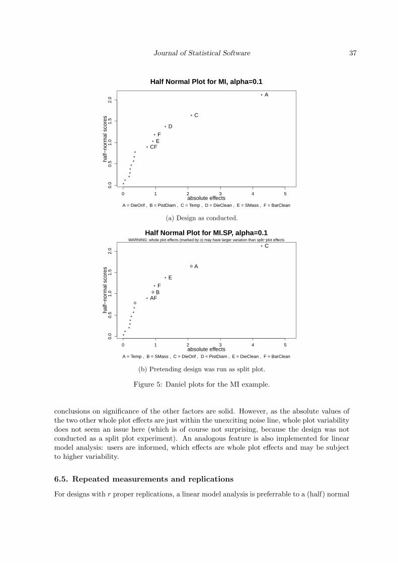
Journal of Statistical Software 37
*
*
*
*
*
*
*
*
**
*
*
*
*
*
0 1 2 3 4 5
0.0
0.5
1.0
1.5
2.0
Half Normal Plot for MI, alpha=0.1
absolute effects
half−
norm
al s
core
s
A = DieOrif , B = PistDiam , C = Temp , D = DieClean , E = SMass , F = BarClean
A
C
D
E F
CF
(a) Design as conducted.
o
o
*
*
*
*
o
*
**
*
*
**
*
0 1 2 3 4 5
0.0
0.5
1.0
1.5
2.0
Half Normal Plot for MI.SP, alpha=0.1
absolute effects
half−
norm
al s
core
s
WARNING: whole plot effects (marked by o) may have larger variation than split−plot effects
A = Temp , B = SMass , C = DieOrif , D = PistDiam , E = DieClean , F = BarClean
A
B
C
E
F
AF
(b) Pretending design was run as split plot.
Figure 5: Daniel plots for the MI example.
conclusions on significance of the other factors are solid. However, as the absolute values ofthe two other whole plot effects are just within the unexciting noise line, whole plot variabilitydoes not seem an issue here (which is of course not surprising, because the design was notconducted as a split plot experiment). An analogous feature is also implemented for linearmodel analysis: users are informed, which effects are whole plot effects and may be subjectto higher variability.
6.5. Repeated measurements and replications
For designs with r proper replications, a linear model analysis is preferrable to a (half) normal
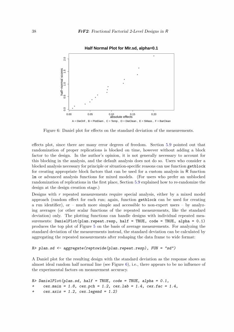
38 FrF2: Fractional Factorial 2-Level Designs in R
*
*
*
*
*
*
*
*
*
*
*
*
*
*
*
0.00 0.05 0.10 0.15 0.20
0.0
0.5
1.0
1.5
2.0
Half Normal Plot for MIr.sd, alpha=0.1
absolute effects
half−
norm
al s
core
s
A = DieOrif , B = PistDiam , C = Temp , D = DieClean , E = SMass , F = BarClean
Figure 6: Daniel plot for effects on the standard deviation of the measurements.
effects plot, since there are many error degrees of freedom. Section 5.9 pointed out thatrandomization of proper replications is blocked on time, however without adding a blockfactor to the design. In the author’s opinion, it is not generally necessary to account forthis blocking in the analysis, and the default analysis does not do so. Users who consider ablocked analysis necessary for principle or situation-specific reasons can use function getblock
for creating appropriate block factors that can be used for a custom analysis in R functionlm or advanced analysis functions for mixed models. (For users who prefer an unblockedrandomization of replications in the first place, Section 5.9 explained how to re-randomize thedesign at the design creation stage.)
Designs with r repeated measurements require special analysis, either by a mixed modelapproach (random effect for each run; again, function getblock can be used for creatinga run identifier), or – much more simple and accessible to non-expert users – by analyz-ing averages (or other scalar functions of the repeated measurements, like the standarddeviation) only. The plotting functions can handle designs with individual repeated mea-surements: DanielPlot(plan.repeat.resp, half = TRUE, code = TRUE, alpha = 0.1)
produces the top plot of Figure 5 on the basis of average measurements. For analyzing thestandard deviation of the measurements instead, the standard deviation can be calculated byaggregating the repeated measurements after reshaping the data frame to wide format:
R> plan.sd <- aggregate(reptowide(plan.repeat.resp), FUN = "sd")
A Daniel plot for the resulting design with the standard deviation as the response shows analmost ideal random half normal line (see Figure 6), i.e., there appears to be no influence ofthe experimental factors on measurement accuracy.
R> DanielPlot(plan.sd, half = TRUE, code = TRUE, alpha = 0.1,
+ cex.main = 1.8, cex.pch = 1.2, cex.lab = 1.4, cex.fac = 1.4,
+ cex.axis = 1.2, cex.legend = 1.2)
Journal of Statistical Software 39
7. Non-regular fractional factorial 2-level designs in FrF2
7.1. Options of function pb
Function pb uses part of the options in complete analogy to those of function FrF2 (seeTable 6). There are only three additional options for special purposes: boxtyssedal (see theonline help), n12.taguchi (see Section 7.3) and oldver (see D.1).
7.2. The implemented arrays
Function pb implements Plackett-Burman designs (Plackett and Burman 1946) with up to100 runs, as introduced in Section 3.5.
Package FrF2 contains a list with generator information for the implemented arrays (pb.list).For some situations, the package uses a different array than the one proposed by Plackett andBurman: the missing 92 run array is created by a Williamson construction, as reported inHedayat, Sloane, and Stufken (1999). Furthermore, for 16, 32 and 64 runs, the alternativedesigns discussed in Section 3.5 are implemented in order to avoid complete aliasing of maineffects and 2fis as much as possible. Table 7 provides an overview of the arrays used infunction pb and summarizes information on their properties which are also discussed in thetext below. D gives some detail on doubling, cycling blocks, and the Williamson construction,especially regarding the column order which deviates from that given in the literature andalso has changed over time in FrF2.
Note that function pb always uses the first m columns of an array for a design in m factors.Thus, the order of the columns in the arrays is very important. The following considerationshave driven the final default ordering of the columns: the 16 run Hadamard matrix and thearrays obtained by doubling or cyclic combination of blocks, as well as the 92 run array (i.e.,the arrays for 40, 52, 56, 64, 76, 88, 92, 96 and 100 runs) contain one column, inclusion of whichdramatically increases aliasing for designs with many factors: this column is completely orheavily partially (for 52, 76 and 100 runs) aliased with various 2fis. This column has thereforebeen moved to the last position of the array, in order to prevent heavy aliasing in screeningdesigns, as long as not all columns are used. For the doubled arrays, the first n/2−1 columnstogether with the afore-mentioned last column yield a resolution IV design; for up to n/2 −1 factors, the design is resolution IV per default, for exactly n/2 factors the option oldver
= TRUE is needed for achieving resolution IV. The arrays created by cyclic combination ofblocks yield almost resolution IV designs (GR > 3.9, with GR from Equation (2)) for up ton/2− 1 factors. The aliasing properties of the arrays are summarized in Table 7.
7.3. Creation and analysis of Plackett-Burman designs
Usage of function pb is straightforward and works analogously to that of function FrF2 forall standard cases. Blocking, split plot designs and estimable 2fis cannot be specified, centerpoints can. Functions lm, DanielPlot and MEPlot have methods for Plackett-Burman designs,and design inspection methods can also be applied.
Usage of function pb is now illustrated using the potato cannon example from Section 3.5.The following commands generate the design and summarize it. The option n12.taguchi =
TRUE makes sure that the design is generated in the Taguchi arrangement, rather than in the
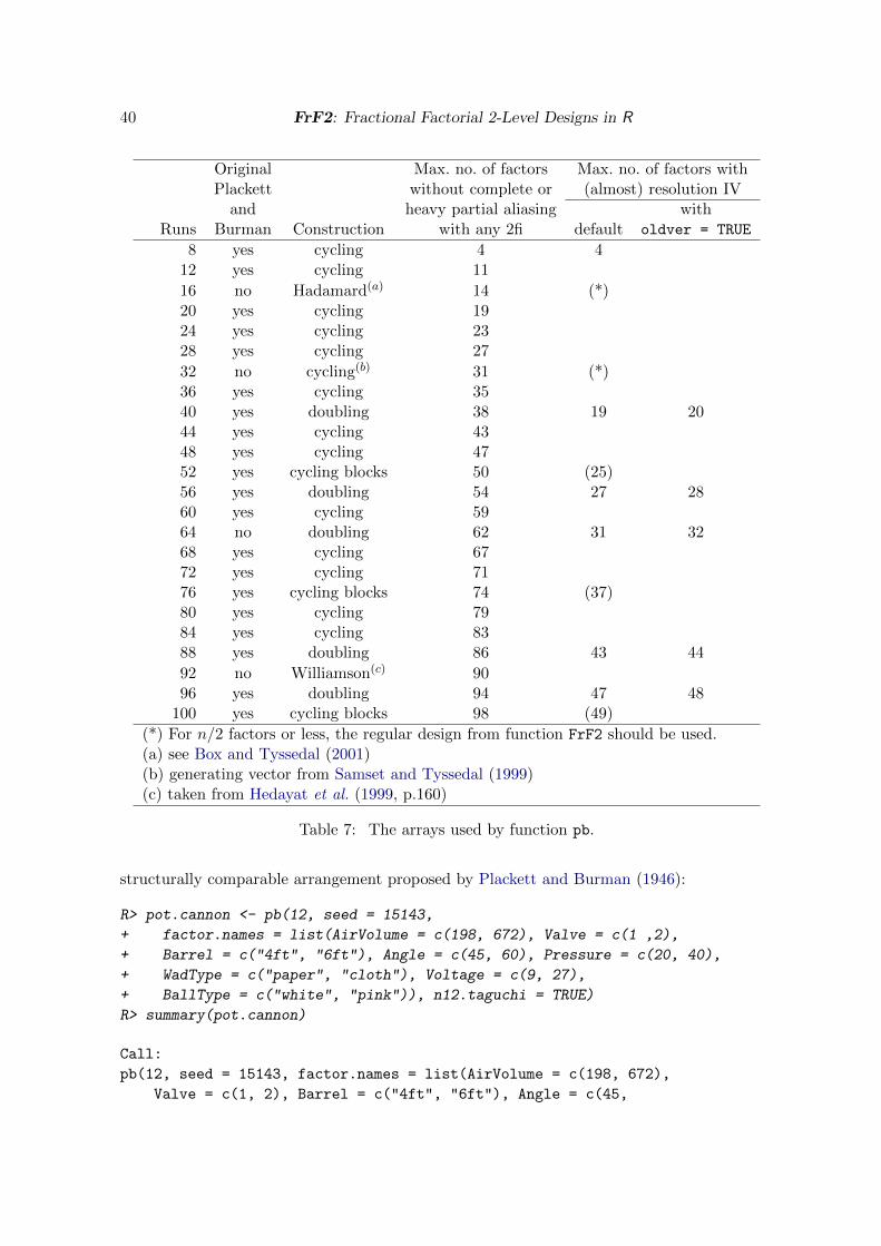
40 FrF2: Fractional Factorial 2-Level Designs in R
Original Max. no. of factors Max. no. of factors withPlackett without complete or (almost) resolution IV
and heavy partial aliasing withRuns Burman Construction with any 2fi default oldver = TRUE
8 yes cycling 4 412 yes cycling 11
16 no Hadamard(a) 14 (*)20 yes cycling 1924 yes cycling 2328 yes cycling 27
32 no cycling(b) 31 (*)36 yes cycling 3540 yes doubling 38 19 2044 yes cycling 4348 yes cycling 4752 yes cycling blocks 50 (25)56 yes doubling 54 27 2860 yes cycling 5964 no doubling 62 31 3268 yes cycling 6772 yes cycling 7176 yes cycling blocks 74 (37)80 yes cycling 7984 yes cycling 8388 yes doubling 86 43 44
92 no Williamson(c) 9096 yes doubling 94 47 48
100 yes cycling blocks 98 (49)
(*) For n/2 factors or less, the regular design from function FrF2 should be used.(a) see Box and Tyssedal (2001)(b) generating vector from Samset and Tyssedal (1999)(c) taken from Hedayat et al. (1999, p.160)
Table 7: The arrays used by function pb.
structurally comparable arrangement proposed by Plackett and Burman (1946):
R> pot.cannon <- pb(12, seed = 15143,
+ factor.names = list(AirVolume = c(198, 672), Valve = c(1 ,2),
+ Barrel = c("4ft", "6ft"), Angle = c(45, 60), Pressure = c(20, 40),
+ WadType = c("paper", "cloth"), Voltage = c(9, 27),
+ BallType = c("white", "pink")), n12.taguchi = TRUE)
R> summary(pot.cannon)
Call:
pb(12, seed = 15143, factor.names = list(AirVolume = c(198, 672),
Valve = c(1, 2), Barrel = c("4ft", "6ft"), Angle = c(45,
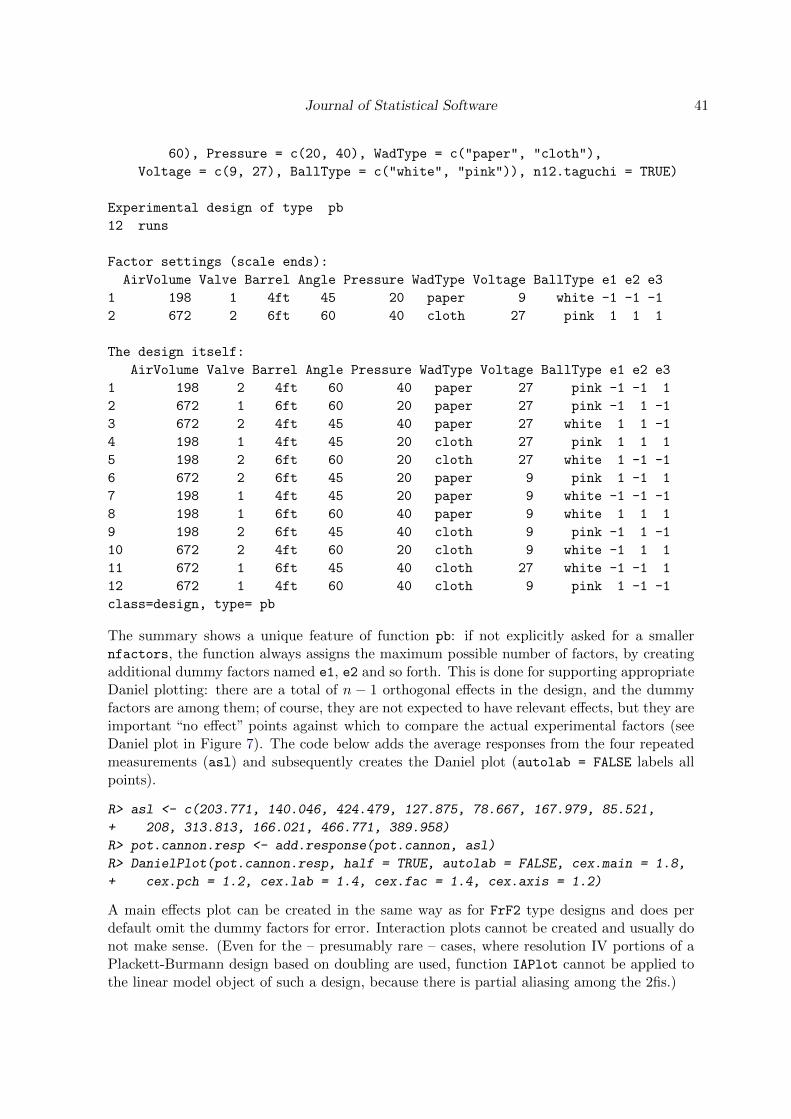
Journal of Statistical Software 41
60), Pressure = c(20, 40), WadType = c("paper", "cloth"),
Voltage = c(9, 27), BallType = c("white", "pink")), n12.taguchi = TRUE)
Experimental design of type pb
12 runs
Factor settings (scale ends):
AirVolume Valve Barrel Angle Pressure WadType Voltage BallType e1 e2 e3
1 198 1 4ft 45 20 paper 9 white -1 -1 -1
2 672 2 6ft 60 40 cloth 27 pink 1 1 1
The design itself:
AirVolume Valve Barrel Angle Pressure WadType Voltage BallType e1 e2 e3
1 198 2 4ft 60 40 paper 27 pink -1 -1 1
2 672 1 6ft 60 20 paper 27 pink -1 1 -1
3 672 2 4ft 45 40 paper 27 white 1 1 -1
4 198 1 4ft 45 20 cloth 27 pink 1 1 1
5 198 2 6ft 60 20 cloth 27 white 1 -1 -1
6 672 2 6ft 45 20 paper 9 pink 1 -1 1
7 198 1 4ft 45 20 paper 9 white -1 -1 -1
8 198 1 6ft 60 40 paper 9 white 1 1 1
9 198 2 6ft 45 40 cloth 9 pink -1 1 -1
10 672 2 4ft 60 20 cloth 9 white -1 1 1
11 672 1 6ft 45 40 cloth 27 white -1 -1 1
12 672 1 4ft 60 40 cloth 9 pink 1 -1 -1
class=design, type= pb
The summary shows a unique feature of function pb: if not explicitly asked for a smallernfactors, the function always assigns the maximum possible number of factors, by creatingadditional dummy factors named e1, e2 and so forth. This is done for supporting appropriateDaniel plotting: there are a total of n − 1 orthogonal effects in the design, and the dummyfactors are among them; of course, they are not expected to have relevant effects, but they areimportant “no effect” points against which to compare the actual experimental factors (seeDaniel plot in Figure 7). The code below adds the average responses from the four repeatedmeasurements (asl) and subsequently creates the Daniel plot (autolab = FALSE labels allpoints).
R> asl <- c(203.771, 140.046, 424.479, 127.875, 78.667, 167.979, 85.521,
+ 208, 313.813, 166.021, 466.771, 389.958)
R> pot.cannon.resp <- add.response(pot.cannon, asl)
R> DanielPlot(pot.cannon.resp, half = TRUE, autolab = FALSE, cex.main = 1.8,
+ cex.pch = 1.2, cex.lab = 1.4, cex.fac = 1.4, cex.axis = 1.2)
A main effects plot can be created in the same way as for FrF2 type designs and does perdefault omit the dummy factors for error. Interaction plots cannot be created and usually donot make sense. (Even for the – presumably rare – cases, where resolution IV portions of aPlackett-Burmann design based on doubling are used, function IAPlot cannot be applied tothe linear model object of such a design, because there is partial aliasing among the 2fis.)
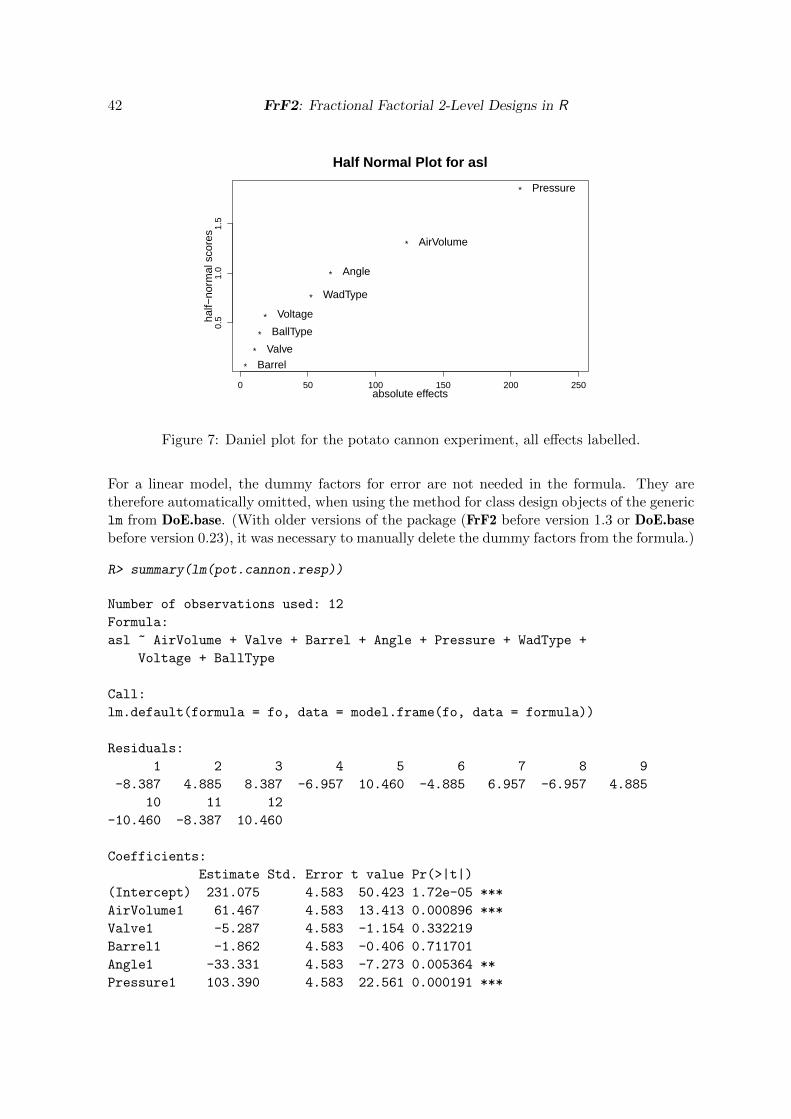
42 FrF2: Fractional Factorial 2-Level Designs in R
*
*
*
*
*
*
*
*
0 50 100 150 200 250
0.5
1.0
1.5
Half Normal Plot for asl
absolute effects
half−
norm
al s
core
s
AirVolume
Valve
Barrel
Angle
Pressure
WadType
Voltage
BallType
Figure 7: Daniel plot for the potato cannon experiment, all effects labelled.
For a linear model, the dummy factors for error are not needed in the formula. They aretherefore automatically omitted, when using the method for class design objects of the genericlm from DoE.base. (With older versions of the package (FrF2 before version 1.3 or DoE.basebefore version 0.23), it was necessary to manually delete the dummy factors from the formula.)
R> summary(lm(pot.cannon.resp))
Number of observations used: 12
Formula:
asl ~ AirVolume + Valve + Barrel + Angle + Pressure + WadType +
Voltage + BallType
Call:
lm.default(formula = fo, data = model.frame(fo, data = formula))
Residuals:
1 2 3 4 5 6 7 8 9
-8.387 4.885 8.387 -6.957 10.460 -4.885 6.957 -6.957 4.885
10 11 12
-10.460 -8.387 10.460
Coefficients:
Estimate Std. Error t value Pr(>|t|)
(Intercept) 231.075 4.583 50.423 1.72e-05 ***
AirVolume1 61.467 4.583 13.413 0.000896 ***
Valve1 -5.287 4.583 -1.154 0.332219
Barrel1 -1.862 4.583 -0.406 0.711701
Angle1 -33.331 4.583 -7.273 0.005364 **
Pressure1 103.390 4.583 22.561 0.000191 ***
Journal of Statistical Software 43
WadType1 26.109 4.583 5.697 0.010722 *
Voltage1 9.193 4.583 2.006 0.138514
BallType1 -7.168 4.583 -1.564 0.215736
---
Signif. codes: 0 '***' 0.001 '**' 0.01 '*' 0.05 '.' 0.1 ' ' 1
Residual standard error: 15.87 on 3 degrees of freedom
Multiple R-squared: 0.9962, Adjusted R-squared: 0.986
F-statistic: 97.78 on 8 and 3 DF, p-value: 0.001539
8. Design augmentation and combination
8.1. Center points and central composite designs
A fractional factorial design can be created with center points (see Section 5.9) or can laterbe augmented with center points by function add.center. (Note that immediate inclusionof center points is preferrable, especially in cases where experimental results may dependon time.) Regular fractional factorial designs, preferrably ones that already contain centerpoints and have at least resolution V, can later be augmented into a central composite design– a special design for response surface exploration (e.g., Montgomery 2001) – using functionccd.augment from DoE.wrapper. This feature is based on the function rsm from rsm (Lenth2009). Note that DoE.wrapper cannot augment split plot designs into central compositedesigns.
8.2. Fold-over
If a fractional factorial design yields ambiguous results because of aliasing of main effects with2fis, ambiguities can be resolved by the fold-over approach, which removes all or certain wordsof length 3. A classical fold-over requires to run another block of the same size as the originalexperiment. Fold-over is covered in various text books, for example Box et al. (2005), Mee(2009) or Montgomery (2001). In FrF2, function fold.design implements fold-over; note,however, that only standard designs can be folded (no center points, no blocked or split plotstructure).
8.3. Robustness designs
Robustness experiments are often conducted using a Taguchi approach with a so-called innerand outer array (see e.g., Montgomery 2001). For the analysis, one often takes aggregatemeasures (e.g., mean, standard deviation or signal-to-noise ratio) over the outer array andanalyzes their dependence on the factors of the inner array. It is possible to create suchexperiments using function param.design from DoE.base. There is some support for au-tomatic calculation of aggregated measures, similar to the tools for designs with repeatedmeasurements (see Section 6.5).
It has been discussed in the literature whether one should conduct robustness experimentsas one large experiment with estimability requirements (as e.g., mentioned in Section 5.7) or
44 FrF2: Fractional Factorial 2-Level Designs in R
whether the inner-outer array approach is more useful. Like so often, the answer depends onthe situation. If robustness can be achieved by exploiting interactions, the combined arrayis often more useful; on the other hand, if there are genuine influences of inner array factorson the variability of the outcome, possibly not even moderated by the outer array factors, aninner-outer array approach is preferable.
9. Further developments
Package FrF2 contains all basic features and many advanced ones for fractional factorial2-level designs. Some further features would still be desirable.
It is possible to create designs with some factors at 4 or 8 levels, based on regular 2-levelfractional factorial designs. So far, such designs are not specifically supported in FrF2. Pack-age DoE.base contains designs with 2-, 4- and 8-level factors, which can be used but do notexplicitly control the alias structure, apart from keeping all main effects orthogonal to eachother. Expert users can use the estimability features for obtaining suitable designs: a resolu-tion III design with one 4-level factor can be obtained by using two 2-level factors and theirinteraction, keeping the interaction estimable with options clear = FALSE and res3 = TRUE;a resolution IV design with one 4-level factor is obtained in the same way, but omitting thesetwo options; a resolution III design with one 8-level factor can be obtained by using three2-level factors for creation of the 8-level factor, making sure that all the 2fis among thesethree factors are kept clear; this also ensures that the 3-factor interaction of the three factorsis not aliased with any main effect. A resolution IV design with two 4-level factors requiresmanual intervention: in addition to keeping the 2fis of the pairs of factors for generating the4-level factors clear, it is necessary to make sure that the four generating factors together donot occur in a word of length 5. Whether or not this is the case can be checked by settingoption alias.info = 3. An analogous approach can also yield a resolution IV design withan 8-level factor. However, in both cases, it is not possible to automatically request the de-sired behavior. It would be desirable to have options for automatic creation of designs withnumber of levels a power of two that also handle the alias structure of the resulting design.However, with the advent of the new package planor, the priority on this improvement hasreduced; it would only be added value if the resulting design could be guaranteed to be bestin some well-defined way, or if finding a design would be much faster (which might be thecase for moderate and large scenarios, at least when considering the current implementationof planor).
Some features are currently not combinable, for example center points with split plot designs,crossing of blocked designs, or estimability requests and blocking. The implementation of allthese combinations requires substantial mathematical and programming work; it will have tobe checked whether it is feasible within the current approaches to blocking, estimability andsplit plotting to achieve any of the combinations with acceptable effort.
There are (not so many) instances for which creation of a clear design is prohibitively slow inthe current implementation that evaluates subgraph isomorphism with the VF2 algorithm byCordella, Foggia, Sansone, and Vento (2001) as implemented in igraph. Recent experienceswith a few of these showed that the LAD algorithm (Solnon 2010) was very fast in ruling outimpossible matches, where VF2 took a long time. Once LAD has been implemented in igraph(it will be part of the next major release), it will replace or complement the VF2 algorithm
Journal of Statistical Software 45
in FrF2, depending on broader experiences to be gained with LAD.
It would be desirable to enhance the automatic analysis features to also include some moreadvanced types, like mixed model analyzes of designs with repeated measurements or splitplot designs. The recently-added function getblock is a first step towards that goal.
References
Addelman C (1962). “Symmetrical and Asymmetrical Fractional Factorial Plans.” Techno-metrics, 4, 47–58.
Bafna SS, Beall AM (1997). “A Design of Experiments Study on the Factors Affecting Variabil-ity in the Melt Index Measurement.” Journal of Applied Polymer Science, 65(2), 277–288.
Barrios E (2012a). BHH2: Useful Functions for Box, Hunter and Hunter II. R packageversion 2012.04-0, URL http://CRAN.R-project.org/package=BHH2.
Barrios E (2012b). BsMD: Bayes Screening and Model Discrimination. R package version0.7-0.1, URL http://CRAN.R-project.org/package=BsMD.
Block R, Mee R (2005). “Resolution IV Designs with 128 Runs.” Journal of Quality Technol-ogy, 37, 282–293.
Block R, Mee R (2006). “Corrigenda.” Journal of Quality Technology, 38, 96.
Box GEP, Hunter JS, Hunter WG (2005). Statistics for Experimenters. 2nd edition. JohnWiley & Sons, New York.
Box GEP, Meyer RD (1993). “Finding the Active Factors in Fractionated Screening Experi-ments.” Journal of Quality Technology, 25, 94–105.
Box GEP, Tyssedal J (2001). “Sixteen Run Designs of High Projectivity for Factor Screening.”Communications in Statistics – Simulation and Computation, 30, 217–228.
Chen J, Sun DX, Wu CFJ (1993). “A Catalogue of Two-Level and Three-Level FractionalFactorial Designs with Small Runs.” International Statistical Review, 61, 131–145.
Cheng CS, Martin RJ, Tang B (1998). “Two-Level Factorial Designs with Extreme Numbersof Level Changes.” The Annals of Statistics, 26, 1522–1539.
Cheng CS, Steinberg DM, Sun DX (1999). “Minimum Aberration and Model Robustness forTwo-Level Fractional Factorial Designs.” Journal of the Royal Statistical Society B, 61,85–93.
Cordella LP, Foggia P, Sansone C, Vento M (2001). “An Improved Algorithm for MatchingLarge Graphs.” In Proceedings of the 3rd IAPR TC-15 Workshop on Graphbased Represen-tations in Pattern Recognition, pp. 149–159.
Csardi G, Nepusz T (2006). “The igraph Software Package for Complex Network Research.”InterJournal, Complex Systems, 1695. URL http://igraph.sf.net/.
46 FrF2: Fractional Factorial 2-Level Designs in R
Daniel C (1959). “Use of Half Normal Plots in Interpreting Two Level Experiments.” Tech-nometrics, 1, 311–340.
Deng LY, Tang B (1999). “Generalized Resolution and Minimum Aberration Criteria forPlackett-Burman and Other Nonregular Factorial Designs.” Statistica Sinica, 9, 1071–1082.
Gromping U (2010). “Clear and Distinct Designs: Two Approaches for Fractional FactorialDesigns with Some Estimable Two-Factor Interactions.” Reports in Mathematics, Physicsand Chemistry 2, Beuth University of Applied Sciences Berlin, Germany.
Gromping U (2011a). “Relative Projection Frequency Tables for Orthogonal Arrays.” Reportsin Mathematics, Physics and Chemistry 1, Beuth University of Applied Sciences Berlin,Germany.
Gromping U (2011b). “Tutorial for Designing Experiments Using the R Package RcmdrPlu-gin.DoE.” Reports in Mathematics, Physics and Chemistry 4, Beuth University of AppliedSciences Berlin, Germany.
Gromping U (2012). “Creating Clear Designs: A Graph-Based Algorithm and a Catalog ofClear Compromise Plans.” IIE Transactions, 44(11), 988–1001.
Gromping U (2013a). “CRAN Task View: Design of Experiments (DoE) & Analysisof Experimental Data.” Version 2013-03-20, URL http://CRAN.R-project.org/view=
ExperimentalDesign.
Gromping U (2013b). DoE.base: Full Factorials, Orthogonal Arrays and Base Utilities forDoE Packages. R package version 0.25-3, URL http://CRAN.R-project.org/package=
DoE.base.
Gromping U (2013c). DoE.wrapper: Wrapper Package for Design of Experiments Function-ality. R package version 0.8-9, URL http://CRAN.R-project.org/package=DoE.wrapper.
Gromping U (2013d). FrF2.catlg128: Catalogues of Resolution IV 128 Run 2-Level Frac-tional Factorials up to 33 Factors That Do Have 5-Letter Words. R package version 1.2-1,URL http://CRAN.R-project.org/package=FrF2.
Gromping U (2013e). RcmdrPlugin.DoE: R Commander Plugin for (Industrial) Designof Experiments. R package version 0.12, URL http://CRAN.R-project.org/package=
RcmdrPlugin.DoE.
Gromping U (2014). FrF2: Fractional Factorial Designs with 2-Level Factors. R packageversion 1.6-9, URL http://CRAN.R-project.org/package=FrF2.
Hedayat AS, Sloane NJ, Stufken J (1999). Orthogonal Arrays: Theory and Applications.Springer-Verlag, New York.
Ke W, Tang B, Wu H (2005). “Compromise Plans with Clear Two-Factor Interactions.”Statistica Sinica, 15, 709–715.
Kobilinsky A, Bouvier A, Monod H (2013). planor: Generation of Regular Factorial Designs.R package version 0.1-5, URL http://CRAN.R-project.org/package=planor.
Journal of Statistical Software 47
Lenth R (1989). “Quick and Easy Analysis of Unreplicated Factorials.” Technometrics, 31,469–473.
Lenth RV (2009). “Response-Surface Methods in R, Using rsm.” Journal of Statistical Soft-ware, 32(7), 1–17. URL http://www.jstatsoft.org/v32/i07/.
Mayfield P (2007). “Potato Cannons and the Taguchi L12: A Design of Experiments CaseStudy.” URL http://www.sigmazone.com/Taguchi_L12_SpudGun.htm.
Mee R (2009). A Comprehensive Guide to Factorial Two-Level Experimentation. Springer-Verlag, New York.
Montgomery D (2001). Design and Analysis of Experiments. 5th edition. John Wiley & Sons,New York.
Plackett RL, Burman JP (1946). “The Design of Optimum Multifactorial Experiments.”Biometrika, 33(4), 305–325.
R Core Team (2013). R: A Language and Environment for Statistical Computing. R Foun-dation for Statistical Computing, Vienna, Austria. ISBN 3-900051-07-0, URL http:
//www.R-project.org/.
Roth T (2013). qualityTools: Statistical Methods for Quality Science. R package version1.54, URL http://CRAN.R-project.org/package=qualityTools.
Ryan KJ, Bulutoglu DA (2010). “Minimum Aberration Fractional Factorial Designs withLarge N .” Technometrics, 52, 250–255.
Samset O, Tyssedal J (1999). “Two-Level Designs with Good Projection Properties.” Technicalreport 12, department of mathematical sciences, The Norwegian University of Science andTechnology, Norway.
Sanchez SM, Sanchez PJ (2005). “Very Large Fractional Factorial and Central CompositeDesigns.” ACM Transactions on Modeling and Computer Simulation, 15, 362–377.
SAS Institute Inc (2009). SAS/QC User’s Guide. SAS Institute Inc., Cary, NC. URL http:
//www.sas.com/.
Solnon C (2010). “AllDifferent-Based Filtering for Subgraph Isomorphism.” Artificial Intelli-gence, 174(12-13), 850–864.
Sun DX (1993). Estimation Capacity and Related Topics in Experimental Designs. Ph.D.thesis, University of Waterloo, Waterloo, Canada.
Tang B, Deng LY (1999). “Minimum G2-Aberration for Non-Regular Fractional FactorialDesigns.” The Annals of Statistics, 27, 1914–1926.
Wu CFJ, Hamada M (2000). Experiments: Planning, Analysis, and Parameter Design Opti-mization. John Wiley & Sons, New York.
Wu H, Mee R, Tang B (2012). “Fractional Factorial Designs with Admissible Sets of ClearTwo-Factor Interactions.” Technometrics, 54(2), 191–197.

48 FrF2: Fractional Factorial 2-Level Designs in R
Wu H, Wu CFJ (2002). “Clear Two-Factor Interactions and Minimum Aberration.” TheAnnals of Statistics, 30, 1496–1511.
Xu H (2009). “Algorithmic Construction of Efficient Fractional Factorial Designs with LargeRun Sizes.” Technometrics, 51(3), 262–277.
Xu H, Wu CFJ (2001). “Generalized Minimum Aberration for Asymmetrical Fractional Fac-torial Designs.” The Annals of Statistics, 29(4), 1066–1077.

Journal of Statistical Software 49
A. Class design and functionality for it
Functions FrF2, FrF2Large and pb create an output design that is of S3 class design andthus follows a certain structure (see Section A.1) and allows application of certain inspection,modification and analysis methods and functions (see Section A.2).
A.1. Class design
An object of S3 class design is a a data frame with the three attributes desnum, run.orderand design.info. All three attributes can be accessed by accessor functions with the samename (e.g., run.order(plan)).
� Attribute desnum contains a numeric version of the data frame, which may be usefulfor users who want to do manual matrix calculations. The package functionality itselfmakes little use of that attribute.
� Attribute run.order has the main purpose of always being able to switch back andforth between a standard order (Yates order, see Section 3.1) and the randomized runorder.
� Attribute design.info is a list that contains important information on the design andis heavily used by the methods and functions of packages DoE.base and FrF2. Thisattribute will be described in some detail in A.3.
A.2. Functionality for class design objects
There are inspection methods (print, summary, plot) and analysis methods (lm, DanielPlot,MEPlot, IAPlot) for this class, as well as a subsetting method which is currently useful forreordering designs only.
Furthermore, there are functions useful for inspecting or modifying the content of a classdesign object (design.info, run.order, desnum, generators, aggregate.design (methodfor the generic aggregate), factor.names, response.names, col.remove, fix.design (methodfor the generic fix adapted from package utils), qua.design, change.contr, reptowide,reptolong, paramtowide, undesign, redesign), functions for augmenting a design with fur-ther runs or response data (add.center, add.response, ccd.augment, fold.design), andfunctions for combining class design objects (cross.design, param.design).
A.3. The design.info attribute
The design.info attribute has some mandatory elements that have to be present for allclass design objects and many elements that are needed for some types of designs only.The author’s web page contains a large table that details which types of designs need whichelements of the design.info attribute (http://prof.beuth-hochschule.de/fileadmin/user/groemping/downloads/classDesignOverviewStructure.pdf). Table 8 lists the ele-ments relevant for designs created with FrF2.
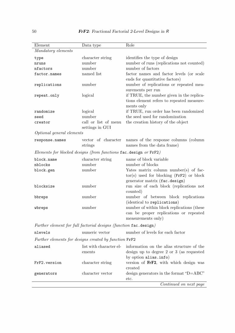
50 FrF2: Fractional Factorial 2-Level Designs in R
Element Data type Role
Mandatory elements
type character string identifies the type of designnruns number number of runs (replications not counted)nfactors number number of factorsfactor.names named list factor names and factor levels (or scale
ends for quantitative factors)replications number number of replications or repeated mea-
surements per runrepeat.only logical if TRUE, the number given in the replica-
tions element refers to repeated measure-ments only
randomize logical if TRUE, run order has been randomizedseed number the seed used for randomizationcreator call or list of menu
settings in GUIthe creation history of the object
Optional general elements
response.names vector of characterstrings
names of the response columns (columnnames from the data frame)
Elements for blocked designs (from functions fac.design or FrF2)
block.name character string name of block variablenblocks number number of blocksblock.gen number Yates matrix column number(s) of fac-
tor(s) used for blocking (FrF2) or blockgenerator matrix (fac.design)
blocksize number run size of each block (replications notcounted)
bbreps number number of between block replications(identical to replications)
wbreps number number of within block replications (thesecan be proper replications or repeatedmeasurements only)
Further element for full factorial designs (function fac.design)
nlevels numeric vector number of levels for each factor
Further elements for designs created by function FrF2
aliased list with character el-ements
information on the alias structure of thedesign up to degree 2 or 3 (as requestedby option alias.info)
FrF2.version character string version of FrF2, with which design wascreated
generators character vector design generators in the format “D=ABC”etc.
Continued on next page
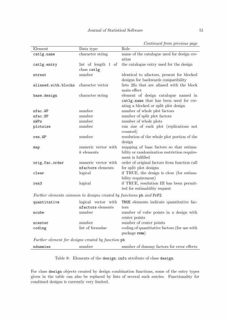
Journal of Statistical Software 51
Continued from previous page
Element Data type Role
catlg.name character string name of the catalogue used for design cre-ation
catlg.entry list of length 1 ofclass catlg
the catalogue entry used for the design
ntreat number identical to nfactors, present for blockeddesigns for backwards compatibility
aliased.with.blocks character vector lists 2fis that are aliased with the blockmain effect
base.design character string element of design catalogue named incatlg.name that has been used for cre-ating a blocked or split plot design
nfac.WP number number of whole plot factorsnfac.SP number number of split plot factorsnWPs number number of whole plotsplotsize number run size of each plot (replications not
counted)res.WP number resolution of the whole plot portion of the
designmap numeric vector with
k elementsmapping of base factors so that estima-bility or randomization restriction require-ment is fulfilled
orig.fac.order numeric vector withnfactors elements
order of original factors from function callfor split plot designs
clear logical if TRUE, the design is clear (for estima-bility requirement)
res3 logical if TRUE, resolution III has been permit-ted for estimability request
Further elements common to designs created by functions pb and FrF2
quantitative logical vector withnfactors elements
TRUE elements indicate quantitative fac-tors
ncube number number of cube points in a design withcenter points
ncenter number number of center pointscoding list of formulae coding of quantitative factors (for use with
package rsm)
Further element for designs created by function pb
ndummies number number of dummy factors for error effects
Table 8: Elements of the design.info attribute of class design.
For class design objects created by design combination functions, some of the entry typesgiven in the table can also be replaced by lists of several such entries. Functionality forcombined designs is currently very limited.
52 FrF2: Fractional Factorial 2-Level Designs in R
B. Exporting designs and importing experimental data
For actual usage of an experimental design package, it is crucial that the R user (who mayor may not be the experimenter) can easily customize the design for actual data collection.In many cases, data collection happens with a spreadsheet software rather than with R.Therefore, data export and import are important. Specifically, for making full use of thepackages’ functionality, it is necessary to preserve the class design information and to addadequate response information to the design.info attribute of the design.
This can be done using the functions export.design for exporting the actual design to a csv
or html file. It is strongly recommended to also save an rda file with the current state of theexperimental design R object. This R object can later be used for adding response data to itwith function add.response.
Function export.design exports a design in the desired format, function add.response canbe used for re-importing it. Details can be found in the online help. The code example belowshows the general principle. Of course, settings have to be adapted to the user’s computersystem, e.g., the InDec and OutDec options that influence the decimal separator and separatorsettings.
R> getwd()
R> des <- FrF2(8, 4)
R> export.design(des, filename = "des", type = "all", OutDec = ",")
This export command writes the three files ‘des.rda’, ‘des.csv’ and ‘des.html’ to the cur-rent R working directory (the location could have been changed by the path option of functionexport.design). The OutDec = "," option corresponds to the R csv2 command for Euro-pean csv settings for the author’s German computer. The csv or html file can be used forcollecting response data. The actual re-import of the response data into R must use a csv file(but the html file could be stored as csv after inputting data). With the same active workingdirectory as before, the following command can re-import the data, after responses have beenadded:
R> des.resp <- add.response("des", "des.withresponses.csv",
+ rdapath = "des.rda", InDec = ",")
This command reads the design des from the rda file des.rda and adds the response valuesfrom the csv file to it (provided, there are no obvious mismatches between the files in whichcase an error message will result).
C. Class catlg and methods for it
The catalogue catlg available in FrF2 contains an ordered list of experimental designs, asdetailed in Section 3.2. Each entry is a list, for example:
R> catlg[["8-4.2"]]
$res
[1] 3
Journal of Statistical Software 53
$nfac
[1] 8
$nruns
[1] 16
$gen
[1] 3 5 9 14
$WLP
[1] 0 0 3 7 4 0 1
$nclear.2fis
[1] 1
$clear.2fis
[,1]
[1,] 1
[2,] 8
$all.2fis.clear
numeric(0)
$dominating
[1] TRUE
The entire list has the class catlg, for which there are a print method, a subsetting method,and various accessor methods (named in most cases after the list element they access). Thesubsetting method makes sure that the ‘[’ subsetting retains the class properties. The effectof the print method can be observed by observing the difference of the previous output tothe one shown now:
R> catlg["8-4.2"]
Design: 8-4.2
16 runs, 8 factors,
Resolution III
Generating columns: 3 5 9 14
WLP (3plus): 3 7 4 0 1 , 1 clear 2fis
Besides affecting the way catalogue elements are printed, the print method also has selectionoptions regarding the number of runs, the number of factors or the resolution of a design.Details can be found in the online help (?print.catlg).
As an example for application of an accessor method, the following code provides the resolutionfor each of the 13 designs of Table 4:
R> res(catlg[1:13])
54 FrF2: Fractional Factorial 2-Level Designs in R
3-1.1 4-1.1 4-1.2 5-2.1 6-3.1 7-4.1 5-1.1 5-1.2 5-1.3 6-2.1 6-2.2 6-2.3
3 4 3 3 3 3 5 4 3 4 3 3
6-2.4
3
Instead of an accessor for the gen element, there is a generators method for class catlg,which allows to print the generators in more human-friendly form, here for all catalogueddesigns in 16 runs for 6 factors:
R> generators(catlg[10:13])
$`6-2.1`
[1] "E=ABC" "F=ABD"
$`6-2.2`
[1] "E=AB" "F=ACD"
$`6-2.3`
[1] "E=AB" "F=CD"
$`6-2.4`
[1] "E=AB" "F=AC"
The catalogue catlg is the default catalogue used by function FrF2. A different cataloguecan be selected with the option select.catlg, for example a catalogue from FrF2.catlg128,or a subset from catlg for continuing a previously successless search for a design with certainestimability requirements (omitting the designs that have already been searched and thusslowly moving forward towards success in case of large important problems). Note thatFrF2.catlg128 must be installed but need not be loaded; if one of its catalogues is requestedby function FrF2, the function automatically loads that package and the relevant catalogue.
D. Column ordering aspects for Plackett-Burman designs
D.1. Designs based on doubling
Starting from an array D with n rows and n/2 − 1 columns, an array in 2n rows and 2n −1 columns can be obtained by doubling. Doubling has some history in FrF2. Versions before1.0-5 used the following arrangement:(
D −D 1D D −1
).
The placement of the column of plus one and minus one vectors last is very beneficial, becausethat vector is the negative product of n/2−1 pairs of the n−1 columns of the doubled design(column 1 with column n/2, column 2 with column n/2+1 etc.). Hence, whenever this columnis among the design columns, there is severe complete aliasing, so that including it last keeps
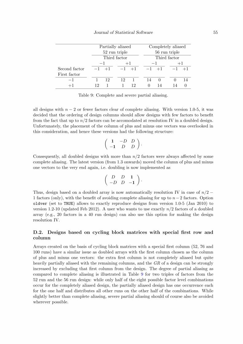
Journal of Statistical Software 55
Partially aliased Completely aliased52 run triple 56 run tripleThird factor Third factor−1 +1 −1 +1
Second factor −1 +1 −1 +1 −1 +1 −1 +1First factor
−1 1 12 12 1 14 0 0 14+1 12 1 1 12 0 14 14 0
Table 9: Complete and severe partial aliasing.
all designs with n − 2 or fewer factors clear of complete aliasing. With version 1.0-5, it wasdecided that the ordering of design columns should allow designs with few factors to benefitfrom the fact that up to n/2 factors can be accomodated at resolution IV in a doubled design.Unfortunately, the placement of the column of plus and minus one vectors was overlooked inthis consideration, and hence these versions had the following structure:(
1 −D D−1 D D
).
Consequently, all doubled designs with more than n/2 factors were always affected by somecomplete aliasing. The latest version (from 1.3 onwards) moved the column of plus and minusone vectors to the very end again, i.e. doubling is now implemented as(
D D 1−D D −1
).
Thus, design based on a doubled array is now automatically resolution IV in case of n/2 −1 factors (only), with the benefit of avoiding complete aliasing for up to n−2 factors. Optionoldver (set to TRUE) allows to exactly reproduce designs from version 1.0-5 (Jan 2010) toversion 1.2-10 (updated Feb 2012). A user who wants to use exactly n/2 factors of a doubledarray (e.g., 20 factors in a 40 run design) can also use this option for making the designresolution IV.
D.2. Designs based on cycling block matrices with special first row andcolumn
Arrays created on the basis of cycling block matrices with a special first column (52, 76 and100 runs) have a similar issue as doubled arrays with the first column chosen as the columnof plus and minus one vectors: the extra first column is not completely aliased but quiteheavily partially aliased with the remaining columns, and the GR of a design can be stronglyincreased by excluding that first column from the design. The degree of partial aliasing ascompared to complete aliasing is illustrated in Table 9 for two triples of factors from the52 run and the 56 run design: while only half of the eight possible factor level combinationsoccur for the completely aliased design, the partially aliased design has one occurrence eachfor the one half and distributes all other runs on the other half of the combinations. Whileslightly better than complete aliasing, severe partial aliasing should of course also be avoidedwherever possible.

56 FrF2: Fractional Factorial 2-Level Designs in R
Furthermore, a design in n/2 factors that only uses the originally odd-numbered columns (i.e.,columns 1, 3, 5, . . . ) is very close to resolution IV (GR > 3.9 in all cases). Thus, startingwith version 1.3 of FrF2, function pb moves the orginally first column to the very end andthe orginally even-numbered columns behind the other originally odd-numbered columns inorder to drastically increase GR for most practically relevant designs. Option oldver can beused for reproducing a design from an earlier version.
D.3. The 92 run design
Finally, the 92 run array also has a similar issue to that of the just-mentioned arrays: its69th column is involved in some triples with heavy aliasing. That column has therefore beenmoved to the very end in order to improve GR for designs with up to 90 factors; again, optionoldver can be used for reproducing the earlier behavior.
Affiliation:
Ulrike GrompingDepartment II – Mathematics, Physics, ChemistryBeuth University of Applied Sciences BerlinD-13353 Berlin, GermanyE-mail: [email protected]: http://prof.beuth-hochschule.de/groemping/
Journal of Statistical Software http://www.jstatsoft.org/
published by the American Statistical Association http://www.amstat.org/
Volume 56, Issue 1 Submitted: 2012-08-16January 2014 Accepted: 2013-04-02

![Fractional Cascading Fractional Cascading I: A Data Structuring Technique Fractional Cascading II: Applications [Chazaelle & Guibas 1986] Dynamic Fractional](https://img.pdfslide.us/doc/110x75/56649ea25503460f94ba64dd/fractional-cascading-fractional-cascading-i-a-data-structuring-technique-fractional.jpg)