R. Douglas Martin* and Ruben H. Zamar**

*Professor of Statistics, Univ. of Washington**Professor of Statistics, Univ. of British Columbia

ROBUST STATISTICS

Key Reference Books

• Huber, P.J. (1981). Robust Statistics, Wiley

• Hampel, F.R., Ronchetti, E.M., Rousseeuw, P.J., and Stahel, W.A. (1986). Robust Statistics, The Approach Based on Influence Functions, Wiley.

• Rousseeuw, P.J. and Leroy, A.M. (1987). Robust Regression and Outlier Detection, Wiley.

J. W. Tukey (1979)

“… just which robust/resistant methods you use is not important – what is important is that you use some. It is perfectly proper to use both classical and robust/resistant methods routinely, and only worry when they differ enough to matter. But when they differ, you should think hard.”

J. W. Tukey“Statistics is a science in my opinion, and it is no more a branch of mathematics than are physics, chemistry and economics; for if its methods fail the test of experience – not the test of logic – they will be discarded”

Recommended reading:

Annals of Statistics Tukey Memorial Volume (Fall, 2002)

“John Tukey’s Contributions to Robust Statistics” (P. J. Huber)

“The Life and Professional Contributions of J. W. Tukey” (D. R. Brillinger)

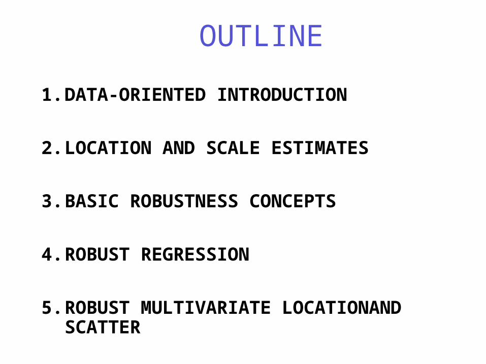
OUTLINE

1. DATA-ORIENTED INTRODUCTION

2. LOCATION AND SCALE ESTIMATES

3. BASIC ROBUSTNESS CONCEPTS

4. ROBUST REGRESSION

5. ROBUST MULTIVARIATE LOCATIONAND SCATTER

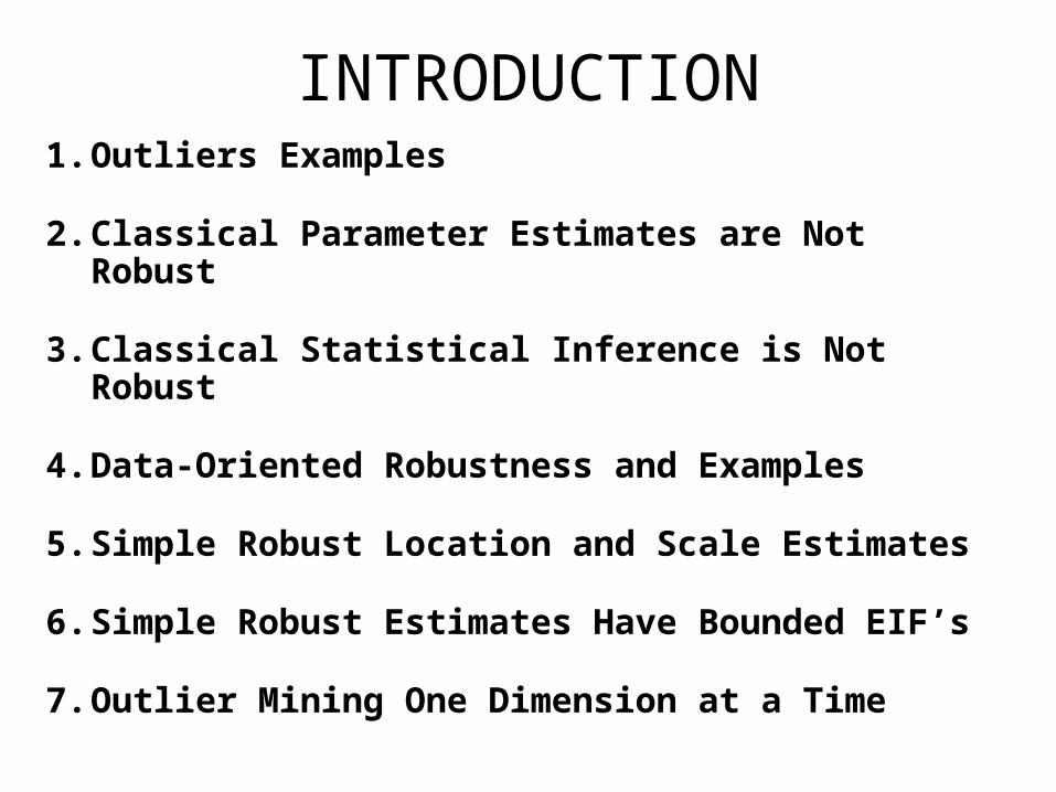
1. Outliers Examples

2. Classical Parameter Estimates are Not Robust

3. Classical Statistical Inference is Not Robust

4. Data-Oriented Robustness and Examples

5. Simple Robust Location and Scale Estimates

6. Simple Robust Estimates Have Bounded EIF’s

7. Outlier Mining One Dimension at a Time

INTRODUCTION

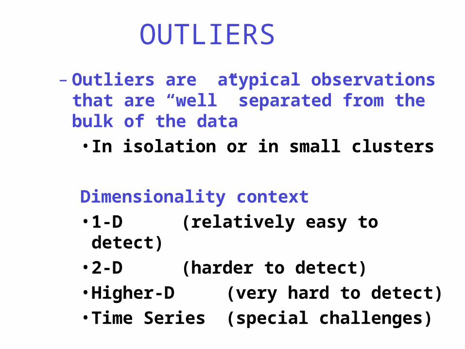
OUTLIERS

– Outliers are atypical observations that are “well” separated from the bulk of the data• In isolation or in small clusters

Dimensionality context• 1-D (relatively easy to

detect)• 2-D (harder to detect)• Higher-D (very hard to detect)• Time Series (special challenges)

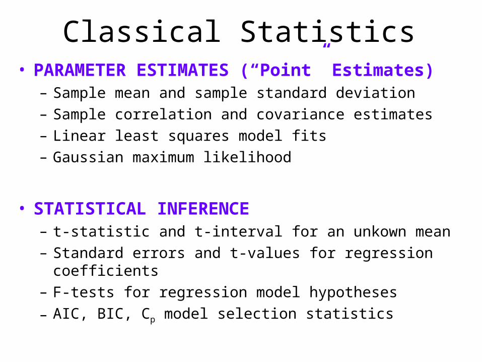
Classical Statistics• PARAMETER ESTIMATES (“Point” Estimates)

– Sample mean and sample standard deviation

– Sample correlation and covariance estimates

– Linear least squares model fits

– Gaussian maximum likelihood

• STATISTICAL INFERENCE– t-statistic and t-interval for an unkown mean

– Standard errors and t-values for regression coefficients

– F-tests for regression model hypotheses

– AIC, BIC, Cp model selection statistics

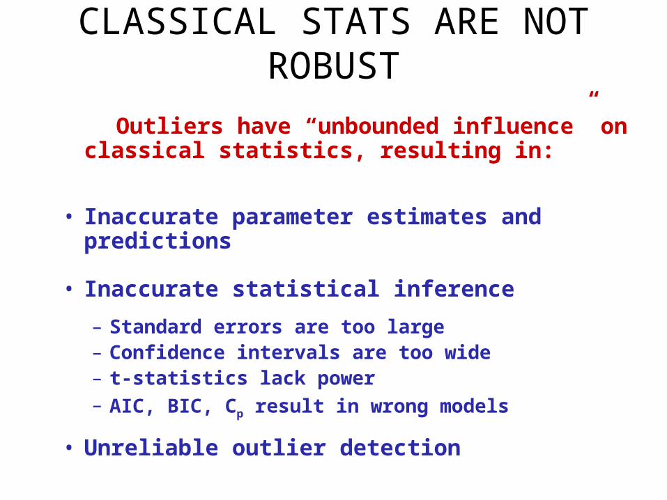
Outliers have “unbounded influence” on classical statistics, resulting in:

• Inaccurate parameter estimates and predictions

• Inaccurate statistical inference

– Standard errors are too large– Confidence intervals are too wide– t-statistics lack power– AIC, BIC, Cp result in wrong models

• Unreliable outlier detection

CLASSICAL STATS ARE NOT ROBUST

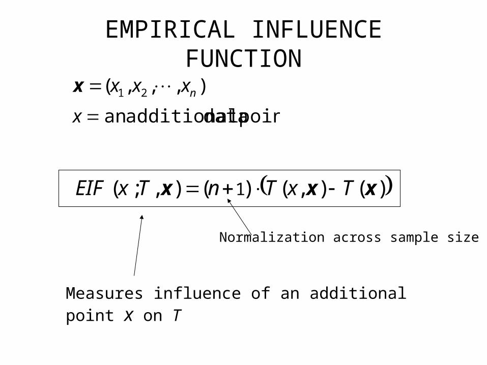
)(),()(),; ( 1 xxx TxTnTxEIF

),,,( 21 nxxx x

point data additionalan x

Normalization across sample size

Measures influence of an additional point x on T

EMPIRICAL INFLUENCE FUNCTION

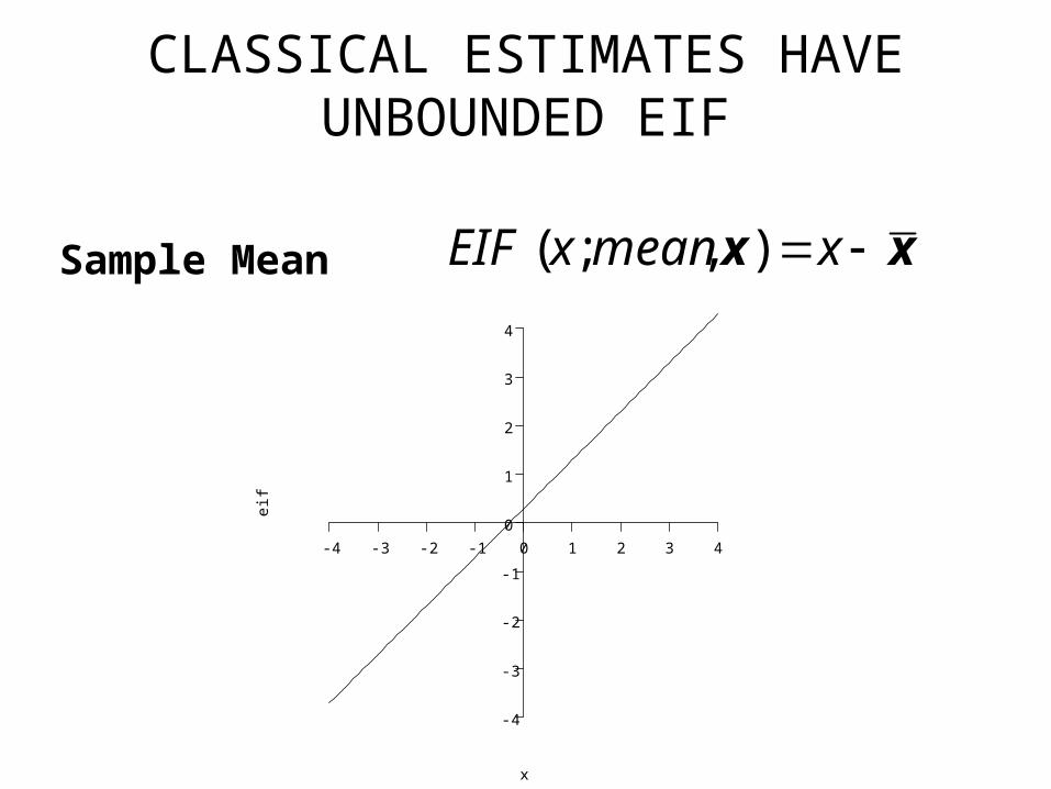
Sample Mean xx xmeanxEIF ),;(

x

eif

-4 -3 -2 -1 0 1 2 3 4

-4

-3

-2

-1

0

1

2

3

4

CLASSICAL ESTIMATES HAVE UNBOUNDED EIF

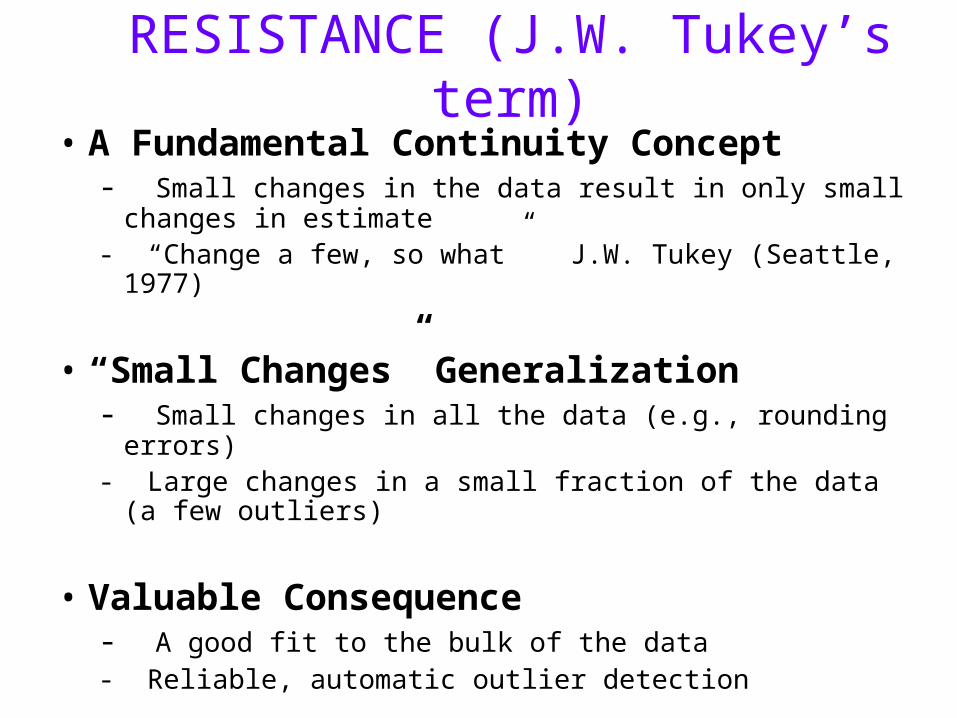
RESISTANCE (J.W. Tukey’s term)

• A Fundamental Continuity Concept- Small changes in the data result in only small changes in

estimate- “Change a few, so what” J.W. Tukey (Seattle, 1977)

• “Small Changes” Generalization- Small changes in all the data (e.g., rounding errors)- Large changes in a small fraction of the data (a few outliers)

• Valuable Consequence- A good fit to the bulk of the data- Reliable, automatic outlier detection

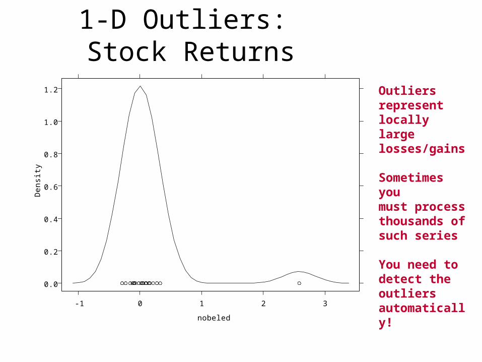
1-D Outliers: Stock Returns

Outliers representlocally largelosses/gains

Sometimes youmust process thousands of such series

You need todetect theoutliersautomatically!0.0

0.2

0.4

0.6

0.8

1.0

1.2

-1 0 1 2 3

nobeled

De

nsi

ty

4.0 4.5 5.0 5.5 6.0

02

46

8

Density of Earth Relative to Density of Water

Density

Outlier

Cavendish, 1798,measurements.

Because of the low outlier the median 5.46 isa better estimateof Earth density than the mean5.42

1-D Outliers: Density of Earth

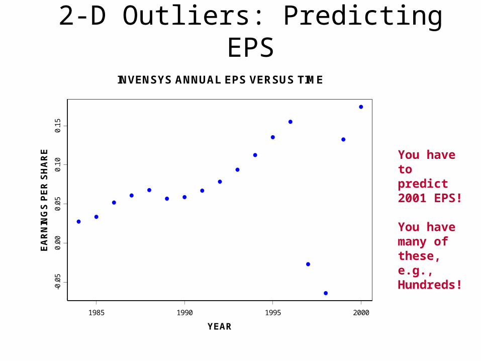
2-D Outliers: Predicting EPS

1985 1990 1995 2000

YEAR

-0.0

50.

000.

050.

100.

15

EA

RN

ING

S P

ER

SH

AR

E

INVENSYS ANNUAL EPS VERSUS TIME

You haveto predict2001 EPS!

You have many of these, e.g.,Hundreds!

-0.85 -0.60 -0.35 -0.10 0.15 0.40 0.65

diff.hstarts

1.0

1.2

1.4

1.6

1.8

2.0

tel.g

ain

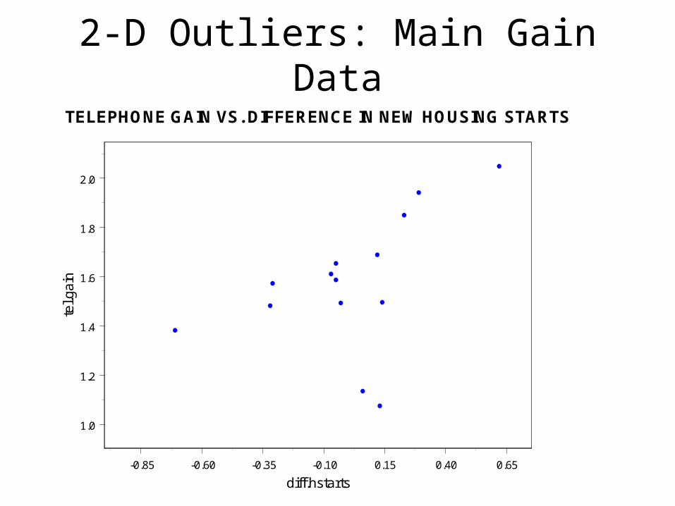
TELEPHONE GAIN VS. DIFFERENCE IN NEW HOUSING STARTS

2-D Outliers: Main Gain Data

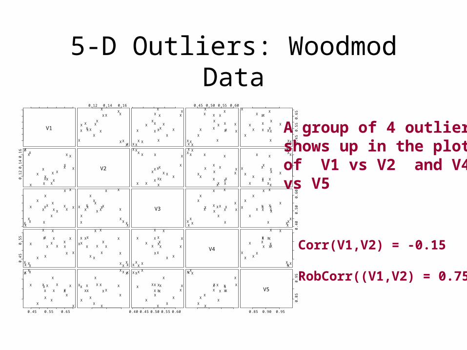
5-D Outliers: Woodmod Data

V1

0.12 0.14 0.16

X

X

X

X

X

X

X

X

X

XX

X

X

X

X X

X

XX

X

X

X

X

X

X

X

X

X

X

XX

X

X

X

XX

X

XX

X

0.45 0.50 0.55 0.60

X

X

X

X

X

X

X

X

X

XXX

X

X

X X

X

XX

X

0.4

50

.55

0.6

5

X

X

X

X

X

X

X

X

X

XX

X

X

X

X X

X

XX

X

0.1

20

.14

0.1

6

X

XX

X

X

X

X

X

X

XX

XX

XX

XX

X

X

X

V2

X

XX

X

X

X

X

X

X

XX

XX

X X

XX

X

X

X X

XX

X

X

X

X

X

X

XX

XX

XX

XX

X

X

X X

XX

X

X

X

X

X

X

XX

XX

XX

XX

X

X

X

X

X

X

X

X

X

X

X

X

X

XX

X

XX

X

XX

XX

X

X

X

X

X

X

X

X

X

X

XX

X

XX

X

XX

XX

V3X

X

X

X

X

X

X

X

X

X

XX

X

XX

X

XX

XX

0.4

00

.50

0.6

0

X

X

X

X

X

X

X

X

X

X

XX

X

XX

X

XX

XX

0.4

50

.55

X XX

X

X

X

XX

X

X

X X

X

XX

X X

X

X

X

X XX

X

X

X

XX

X

X

XX

X

XX

XX

X

X

X

X XX

X

X

X

XX

X

X

XX

X

X X

X X

X

X

X

V4X X

X

X

X

X

XX

X

X

XX

X

XX

X X

X

X

X

0.45 0.55 0.65

X

X

X

X

X

X

X

X

X

X

X

X

XXX

X

X

X

X

X

X

X

X

X

X

X

X

X

X

X

X

X

XXX

X

X

X

X

X

0.40 0.45 0.50 0.55 0.60

X

X

X

X

X

X

X

X

X

X

X

X

XX X

X

X

X

X

X

X

X

X

X

X

X

X

X

X

X

X

X

X XX

X

X

X

X

X

0.85 0.90 0.95

0.8

50

.95

V5

A group of 4 outliersshows up in the plotsof V1 vs V2 and V4vs V5

Corr(V1,V2) = -0.15

RobCorr((V1,V2) = 0.75

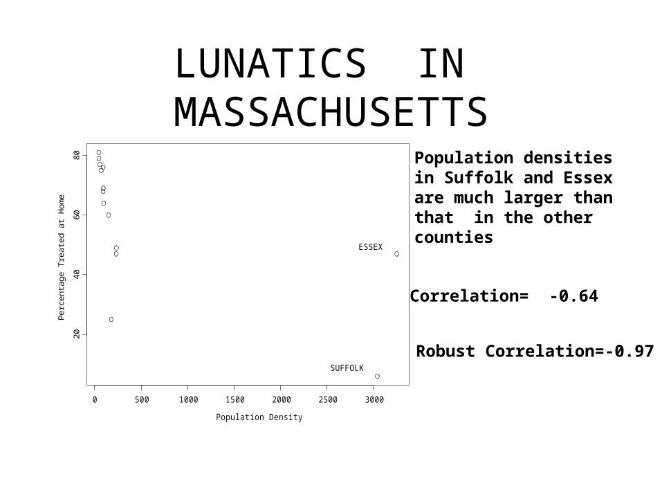
LUNATICS IN MASSACHUSETTS

Population densitiesin Suffolk and Essexare much larger thanthat in the other counties

Correlation= -0.64

Robust Correlation=-0.97

Population Density

Per

cent

age

Trea

ted

at H

ome

0 500 1000 1500 2000 2500 3000

2040

6080

SUFFOLK

ESSEX

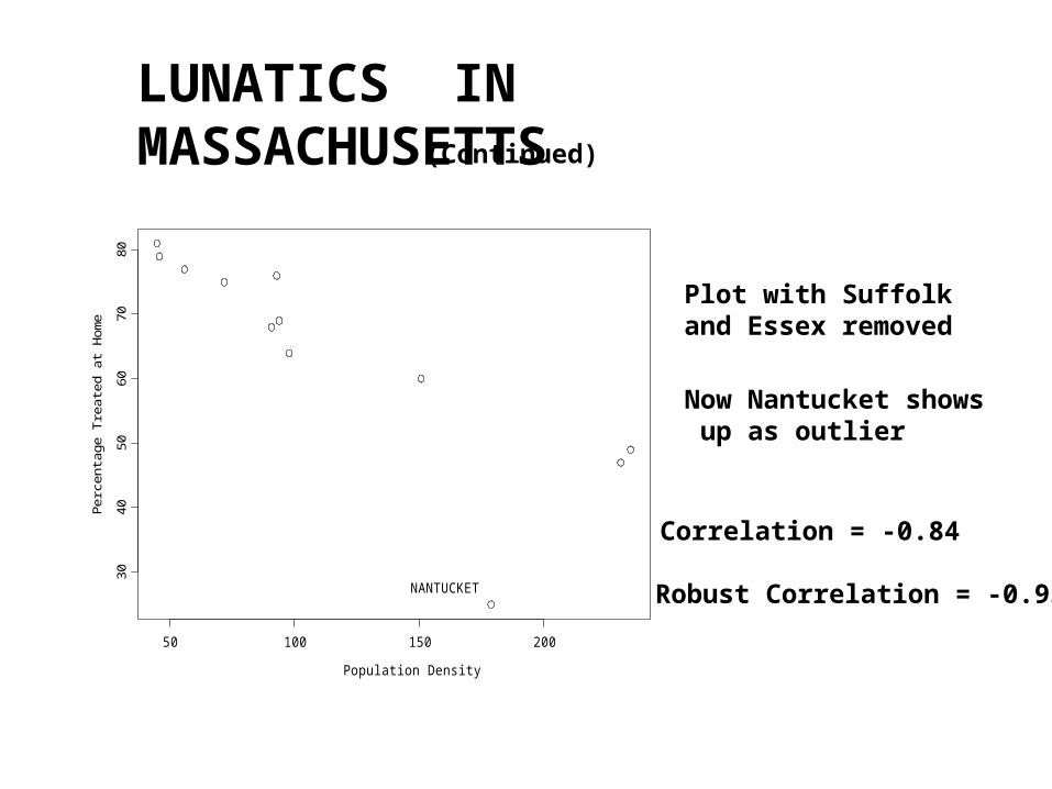
LUNATICS IN MASSACHUSETTS

Now Nantucket shows up as outlier

Plot with Suffolkand Essex removed

Correlation = -0.84

Robust Correlation = -0.93

Population Density

Per

cent

age

Trea

ted

at H

ome

50 100 150 200

3040

5060

7080

NANTUCKET

(Continued)

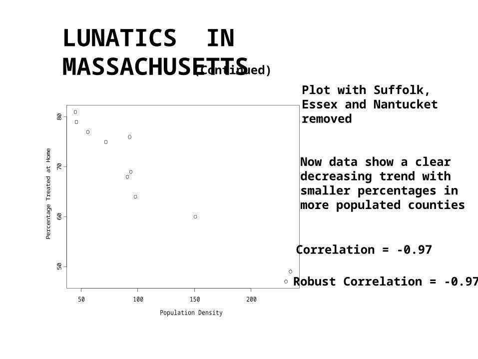
LUNATICS IN MASSACHUSETTS

Plot with Suffolk,Essex and Nantucket removed

Now data show a cleardecreasing trend with smaller percentages inmore populated counties

Correlation = -0.97

Robust Correlation = -0.97

Population Density

Per

cent

age

Trea

ted

at H

ome

50 100 150 200

5060

7080

(Continued)

1955 1956 1957 1958 1959 1960

TIME

70

080

090

010

00

TO

BA

CC

O S

AL

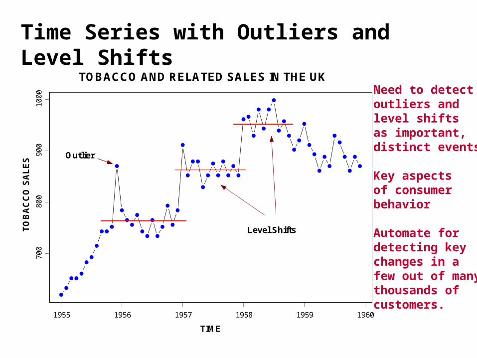
ES Outlier

TOBACCO AND RELATED SALES IN THE UK

Level Shifts

Need to detectoutliers andlevel shiftsas important,distinct events

Key aspectsof consumerbehavior

Automate fordetecting keychanges in afew out of manythousands ofcustomers.

Time Series with Outliers and Level Shifts

Microarray experiments typically used to identify differentially expressed genes.

DNA probes printed on a glass are hybridized to two RNA samples separately labeled with two fluorescent dyes

The intensity of hybridization values after slide scanning

are calculated using image analysis and then used to identify

differentially expressed genes

Gene Expression Data

Array fabrication (pcr amplification and clone preparation, reaction clean up, array printing)

Probe preparation (mRNA extraction, mRNA labeling, probe labeling and purification) and hybridization

Slide scanning and image processing (gridding, segmentation intensity extraction)

Three Principal Stages of the Technology

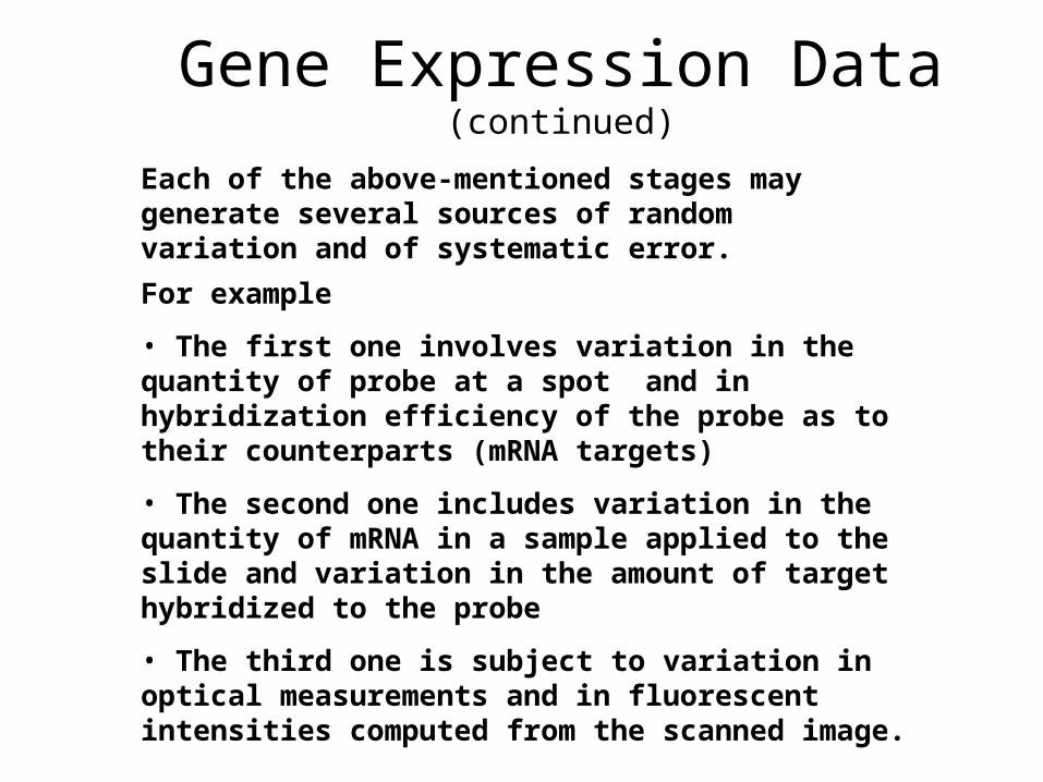
Each of the above-mentioned stages may generate several sources of random variation and of systematic error.

For example

• The first one involves variation in the quantity of probe at a spot and in hybridization efficiency of the probe as to their counterparts (mRNA targets)

• The second one includes variation in the quantity of mRNA in a sample applied to the slide and variation in the amount of target hybridized to the probe

• The third one is subject to variation in optical measurements and in fluorescent intensities computed from the scanned image.

Gene Expression Data(continued)

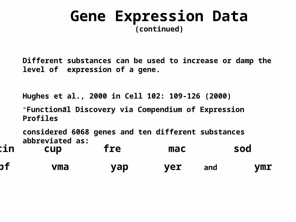
Different substances can be used to increase or damp the level of expression of a gene.

Hughes et al., 2000 in Cell 102: 109-126 (2000)

“Functional Discovery via Compendium of Expression Profiles”

considered 6068 genes and ten different substances abbreviated as:

cin cup fre mac sod

spf vma yap yer and ymr

Gene Expression Data(continued)

Gene Expression Data(continued)

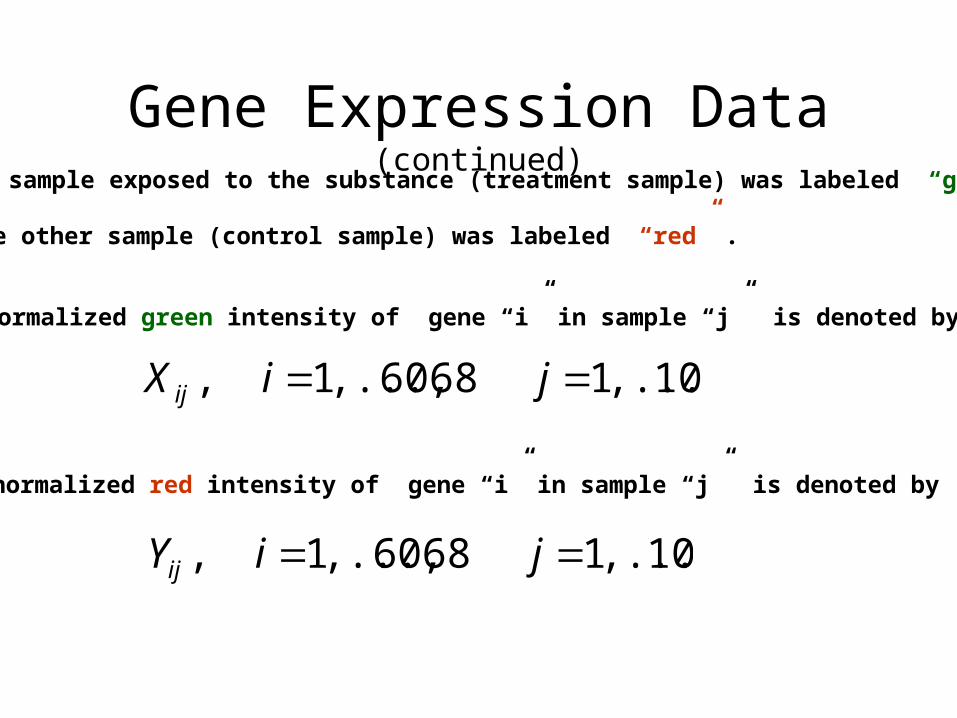
The sample exposed to the substance (treatment sample) was labeled “green”

The other sample (control sample) was labeled “red” .

The normalized green intensity of gene “i” in sample “j” is denoted by

10,...,1 6068,...,1 , jiX ij

The normalized red intensity of gene “i” in sample “j” is denoted by

10,...,1 6068,...,1 , jiYij

Gene Expression Data(continued)

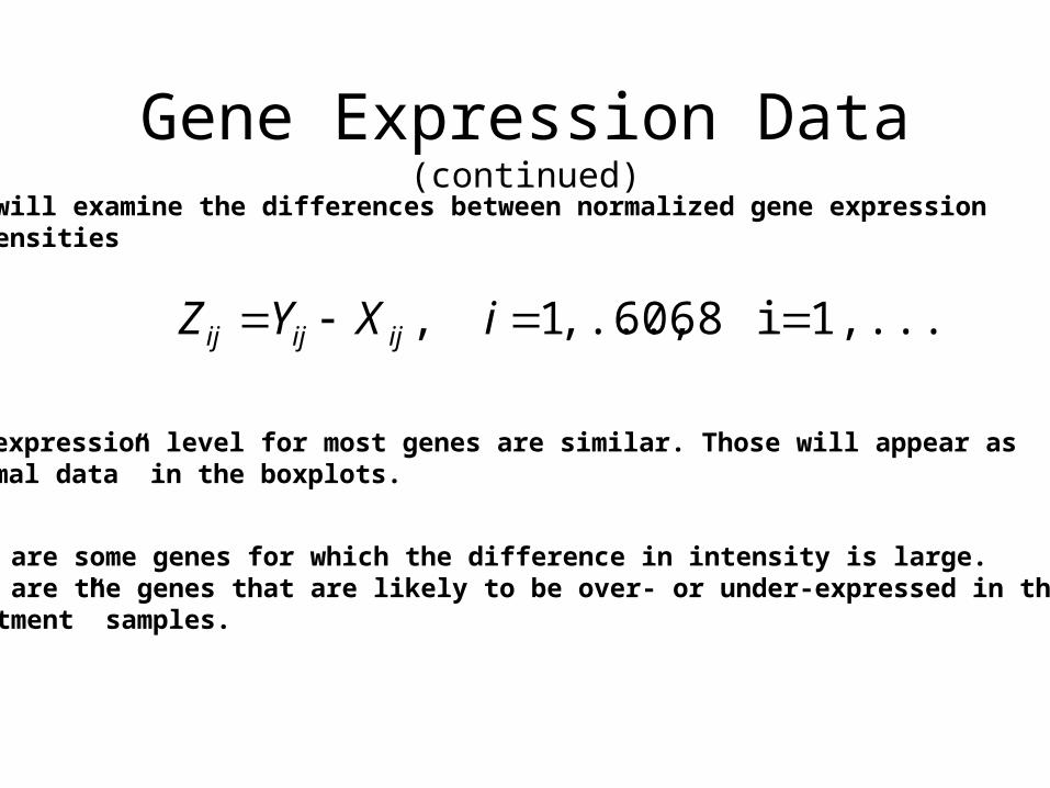
We will examine the differences between normalized gene expression intensities

The expression level for most genes are similar. Those will appear as “normal data” in the boxplots.

1,...,10i 6068,...,1 , iXYZ ijijij

There are some genes for which the difference in intensity is large. Those are the genes that are likely to be over- or under-expressed in the “treatment” samples.

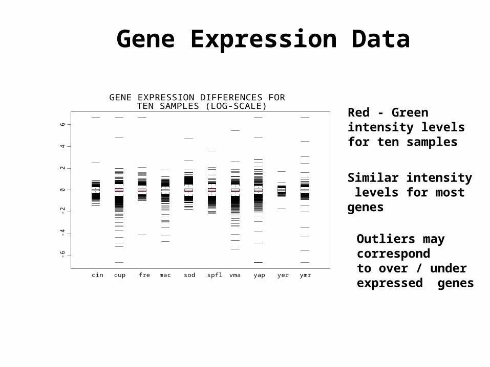
Gene Expression Data

Red - Greenintensity levels for ten samples

Similar intensity levels for mostgenes

-6-4

-20

24

6

cin cup fre mac sod spfl vma yap yer ymr

GENE EXPRESSION DIFFERENCES FOR TEN SAMPLES (LOG-SCALE)

Outliers maycorrespondto over / underexpressed genes

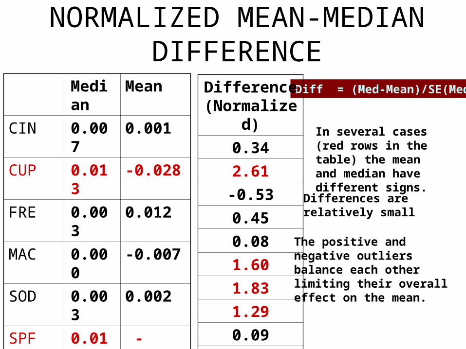
NORMALIZED MEAN-MEDIAN DIFFERENCE

Median

Mean

CIN 0.007 0.001

CUP 0.013 -0.028

FRE 0.003 0.012

MAC 0.000 -0.007

SOD 0.003 0.002

SPF 0.013 -0.012

VMA 0.003 -0.026

YAP 0.010 -0.010

VER 0.003 0.002

VMR 0.000 -0.003

Diff = (Med-Mean)/SE(Med)

In several cases (red rows in the table) the mean and median havedifferent signs.

The positive andnegative outliers balance each otherlimiting their overalleffect on the mean.

Differences are relatively small

Difference (Normalized)

0.34

2.61

-0.53

0.45

0.08

1.60

1.83

1.29

0.09

0.20

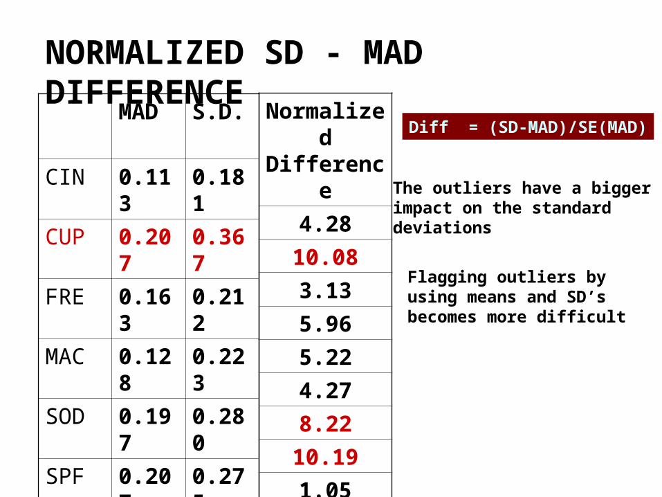
NORMALIZED SD - MAD DIFFERENCE

MAD S.D.

CIN 0.113 0.181

CUP 0.207 0.367

FRE 0.163 0.212

MAC 0.128 0.223

SOD 0.197 0.280

SPF 0.207 0.275

VMA 0.202 0.332

YAP 0.148 0.310

YER 0.069 0.086

YMR 0.113 0.224

Diff = (SD-MAD)/SE(MAD)

The outliers have a bigger impact on the standarddeviations

Flagging outliers byusing means and SD’sbecomes more difficult

Normalized Difference

4.28

10.08

3.13

5.96

5.22

4.27

8.22

10.19

1.05

6.98

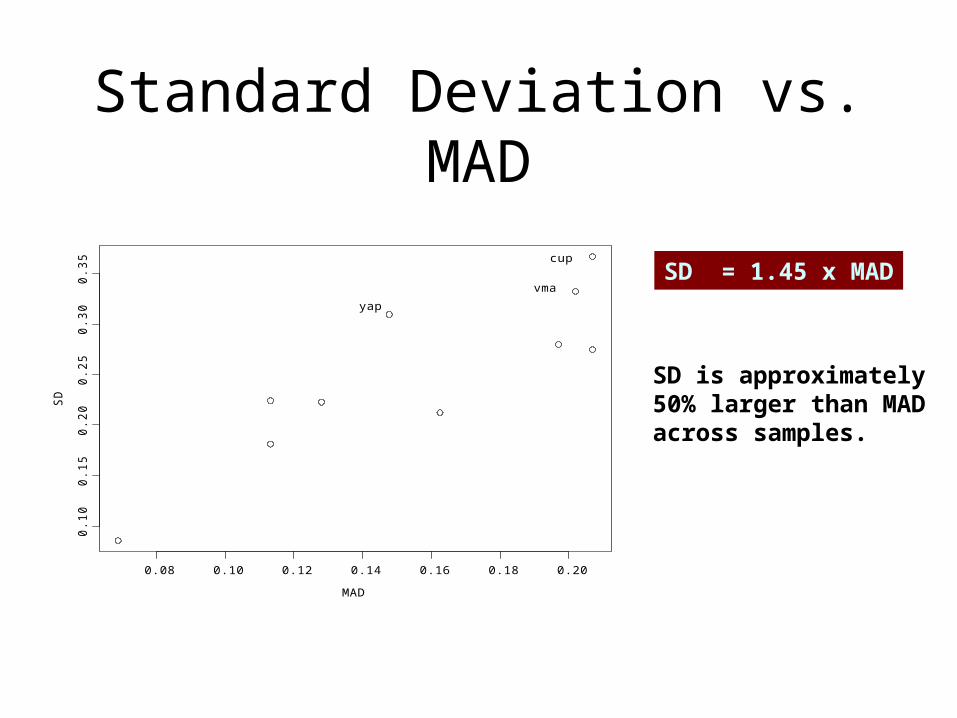
Standard Deviation vs. MAD

SD = 1.45 x MAD

SD is approximately 50% larger than MADacross samples.

MAD

SD

0.08 0.10 0.12 0.14 0.16 0.18 0.20

0.1

00

.15

0.2

00

.25

0.3

00

.35 cup

vma

yap

Flagging Outliers

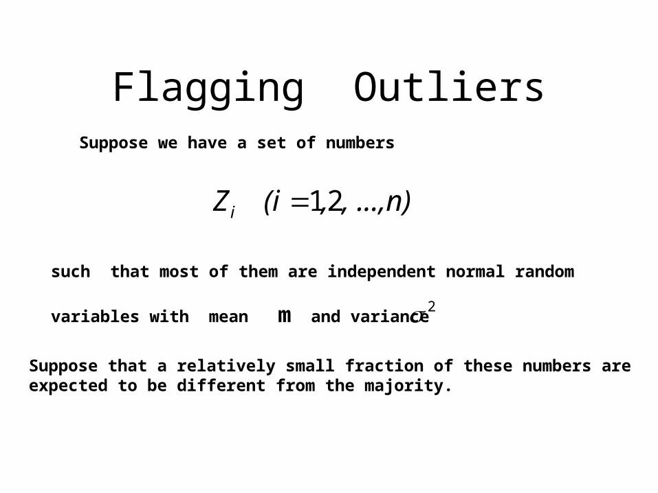
21 , ...,n),(iZi

Suppose we have a set of numbers

such that most of them are independent normal random

variables with mean m and variance 2

Suppose that a relatively small fraction of these numbers are expected to be different from the majority.

Flagging Outliers(continued)

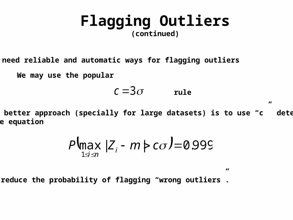
999.0||max1

cmZP ini

We may use the popular

3c

But a better approach (specially for large datasets) is to use “c” determined by the equation

We need reliable and automatic ways for flagging outliers

rule

to reduce the probability of flagging “wrong outliers”.

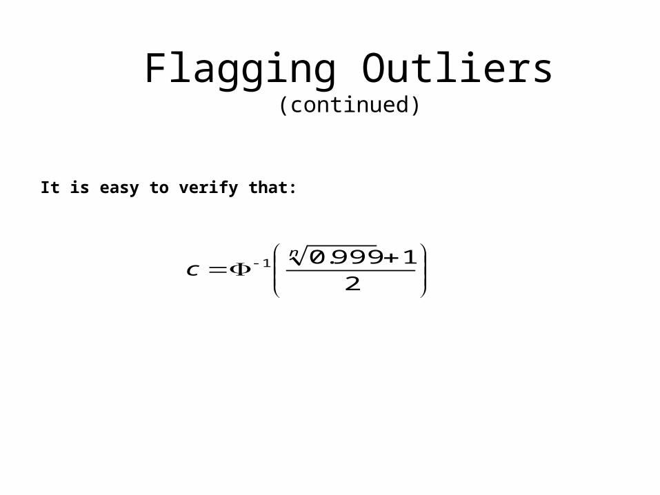
2

1999.01n

c

Flagging Outliers(continued)

It is easy to verify that:

Flagging Outliers(continued)

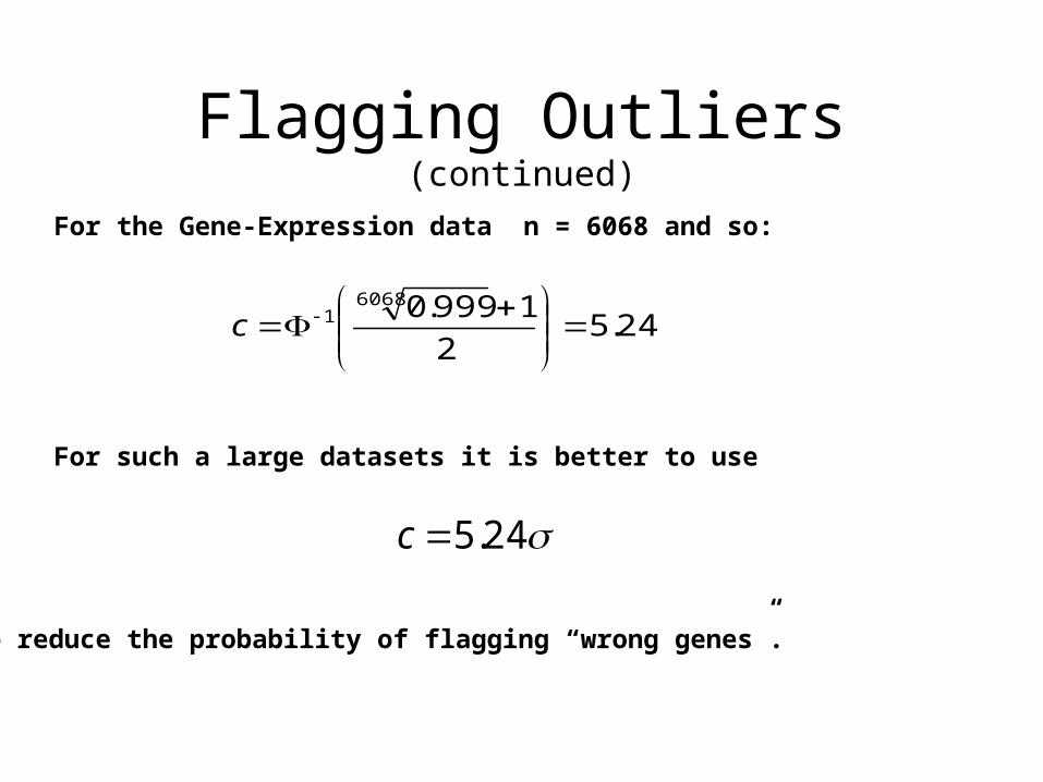
For the Gene-Expression data n = 6068 and so:

24.52

1999.060681

c

For such a large datasets it is better to use

24.5c

to reduce the probability of flagging “wrong genes”.

Flagging Outliers(continued)

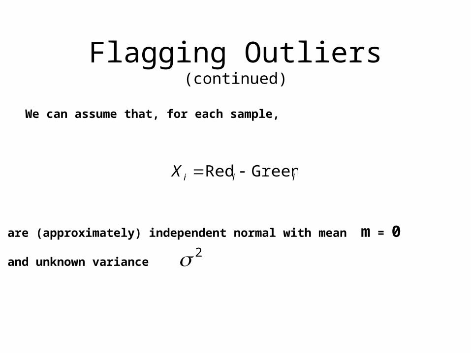
We can assume that, for each sample,

iiiX GreenRed

2are (approximately) independent normal with mean m = 0

and unknown variance

Flagging Outliers(continued)

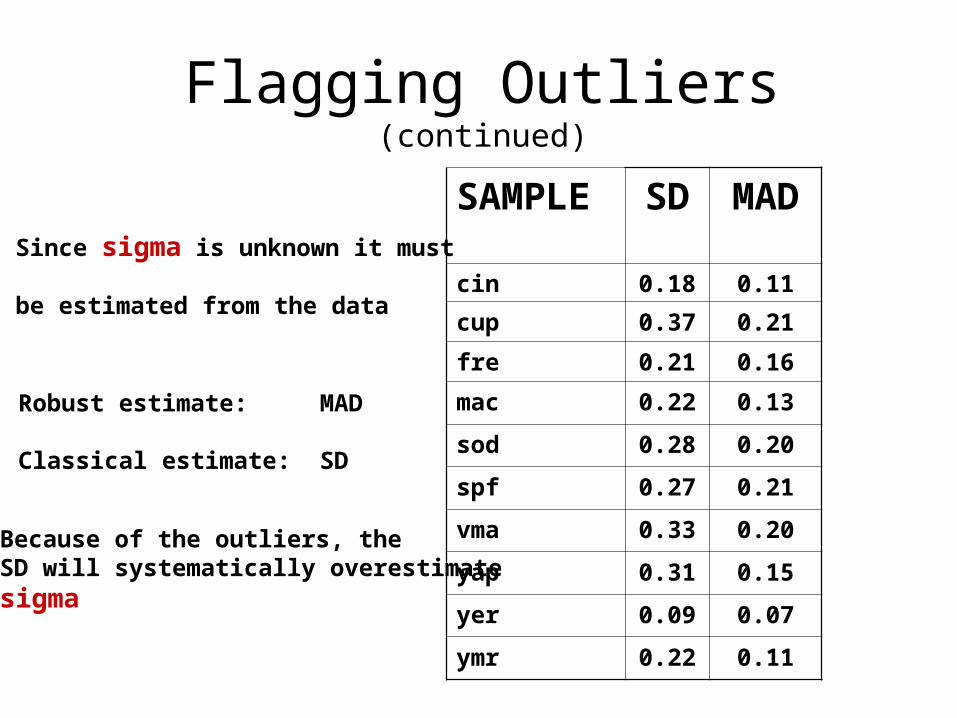
Since sigma is unknown it must be estimated from the data

Robust estimate: MAD

Classical estimate: SD

SAMPLE SD MAD

cin 0.18 0.11

cup 0.37 0.21

fre 0.21 0.16

mac 0.22 0.13

sod 0.28 0.20

spf 0.27 0.21

vma 0.33 0.20

yap 0.31 0.15

yer 0.09 0.07

ymr 0.22 0.11

Because of the outliers, theSD will systematically overestimatesigma

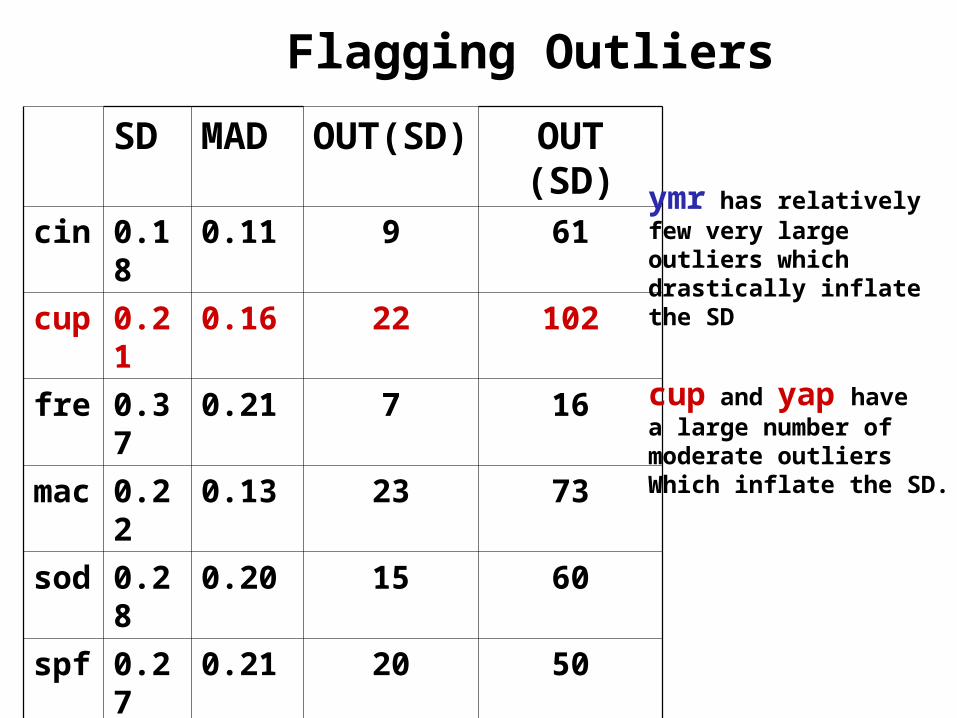
SD MAD OUT(SD) OUT (SD)cin 0.18 0.11 9 61

cup 0.21 0.16 22 102

fre 0.37 0.21 7 16

mac 0.22 0.13 23 73

sod 0.28 0.20 15 60

spf 0.27 0.21 20 50

vma 0.33 0.20 91 27

yap 0.31 0.15 28 114

yer 0.09 0.07 7 18

ymr 0.22 0.11 12 32

ymr has relatively few very large outliers whichdrastically inflate the SD

cup and yap havea large number ofmoderate outliersWhich inflate the SD.

Flagging Outliers

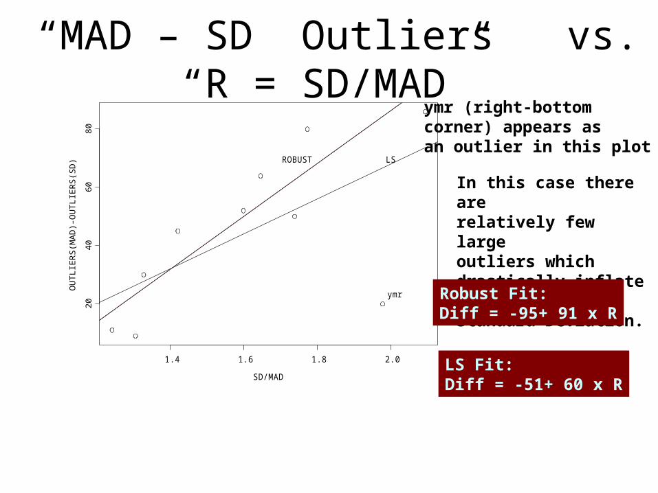
“MAD – SD Outliers” vs. “R = SD/MAD”

ymr (right-bottomcorner) appears as an outlier in this plot

In this case there arerelatively few largeoutliers which drastically inflate theStandard Deviation.

SD/MAD

OU

TLI

ER

S(M

AD

)-O

UT

LIE

RS

(SD

)

1.4 1.6 1.8 2.0

2040

6080

ymr

ROBUST LS

Robust Fit:Diff = -95+ 91 x R

LS Fit:Diff = -51+ 60 x R

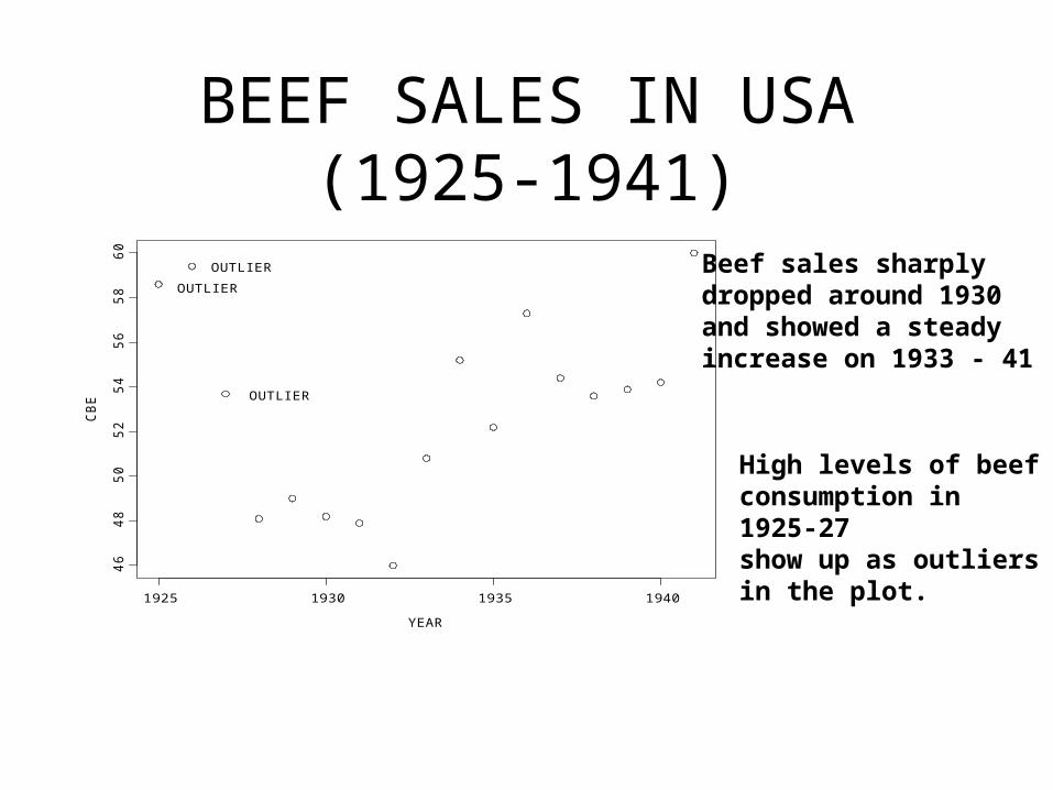
BEEF SALES IN USA (1925-1941)

YEAR

CB

E

1925 1930 1935 1940

46

48

50

52

54

56

58

60

OUTLIER

OUTLIER

OUTLIER

Beef sales sharplydropped around 1930and showed a steadyincrease on 1933 - 41

High levels of beef consumption in 1925-27 show up as outliersin the plot.