Embed Size (px)
Citation preview
Integrated Production-Inventory Models in Steel
Mills Operating in a Fuzzy Environment
Rami Afif As’ad
A Thesis
in
The Department
of
Mechanical and Industrial Engineering
Presented in Partial Fulfillment of the Requirements for the Degree of Doctor of Philosophy (Mechanical Engineering) at
Concordia University Montréal, Québec, Canada
December 2010
©Rami Afif As’ad, 2010

CONCORDIA UNIVERSITY
SCHOOL OF GRADUATE STUDIES This is to certify that the thesis prepared By: Rami Afif As’ad Entitled: Integrated Production Inventory Models in Steel Mills Operating in
a Fuzzy Environment and submitted in partial fulfillment of the requirements for the degree of DOCTOR OF PHILOSOPHY (Mechanical Engineering) complies with the regulations of the University and meets the accepted standards with respect to originality and quality. Signed by the final examining committee:
Chair Prof. B. Jaumard
External Examiner Prof. S. Zolfaghari
External to Program Prof. S. Goyal
Examiner Prof. M. Chen
Examiner Dr. A. Akgunduz
Thesis Supervisor Dr. K. Demirli Approved by
Chair of Department or Graduate Program Director
December 21, 2010 Dean of Faculty

iii
ABSTRACT
Integrated Production-Inventory Models in Steel Mills Operating in a
Fuzzy Environment
Rami Afif As’ad, Ph.D.
Concordia University, 2010
Despite the paramount importance of the steel rolling industry and its vital
contributions to a nation’s economic growth and pace of development, production
planning in this industry has not received as much attention as opposed to other
industries. The work presented in this thesis tackles the master production scheduling
(MPS) problem encountered frequently in steel rolling mills producing reinforced
steel bars of different grades and dimensions. At first, the production planning
problem is dealt with under static demand conditions and is formulated as a mixed
integer bilinear program (MIBLP) where the objective of this deterministic model is
to provide insights into the combined effect of several interrelated factors such as
batch production, scrap rate, complex setup time structure, overtime, backlogging and
product substitution, on the planning decisions.
Typically, MIBLPs are not readily solvable using off-the-shelf optimization
packages necessitating the development of specifically tailored solution algorithms
that can efficiently handle this class of models. The classical linearization approaches
are first discussed and employed to the model at hand, and then a hybrid
linearization-Benders decomposition technique is developed in order to separate the
iv
complicating variables from the non-complicating ones. As a third alternative, a
modified Branch-and-Bound (B&B) algorithm is proposed where the branching,
bounding and fathoming criteria differ from those of classical B&B algorithms
previously established in the literature. Numerical experiments have shown that the
proposed B&B algorithm outperforms the other two approaches for larger problem
instances with savings in computational time amounting to 48%.
The second part of this thesis extends the previous analysis to allow for the
incorporation of internal as well as external sources of uncertainty associated with
end customers’ demand and production capacity in the planning decisions. In such
situations, the implementation of the model on a rolling horizon basis is a common
business practice but it requires the repetitive solution of the model at the beginning
of each time period. As such, viable approximations that result in a tractable number
of binary and/or integer variables and generate only exact schedules are developed.
Computational experiments suggest that a fair compromise between the quality of the
solutions and substantial computational time savings is achieved via the employment
of these approximate models.
The dynamic nature of the operating environment can also be captured using the
concept of fuzzy set theory (FST). The use of FST allows for the incorporation of the
decision maker’s subjective judgment in the context of mathematical models through
flexible mathematical programming (FMP) approach and possibilistic programming
(PP) approach. In this work, both of these approaches are combined where the
volatility in demand is reflected by a flexible constraint expressed by a fuzzy set
having a triangular membership function, and the production capacity is expressed as

v
a triangular fuzzy number. Numerical analysis illustrates the economical benefits
obtained from using the fuzzy approach as compared to its deterministic counterpart.

vi
Dedicated to
… My family …
For their endless love and support, and having always believed in me no matter what
… My fiancée …
For giving my life a whole different meaning and making it so wonderful
I cannot wait to meet with you all after this time that we had to spend apart

vii
AKNOWLEDGMENTS
All praise and thanks are due to GOD for giving me the patience and perseverance
to successfully accomplish my Ph.D. study.
My deepest gratitude is for the two people closest to my heart, mom and dad.
They have always sacrificed their own well being for the sake of mine and done
everything they could to make their kids happy. Their words of encouragement are
unforgettable and I particularly remember them calling me “Dr. Rami” since I was in
the seventh grade. Although a PhD degree in engineering is probably not what they
had in mind, but I hope it still counts! From the bottom of my heart “I love you so
much”. I am also grateful to the other shining starts in my life, my two brothers and
my sister, for always being there for me. Their beautiful kids are the joy of my life.
I won’t forget to thank the person who enlightens my life day after day, my
fiancée. I could not have asked for a better soul mate than her and I cannot wait to
share every moment of my life with her.
I would also like to express my sincere thanks and appreciation to my supervisor
Dr. Kudret Demirli for his continuous support and valuable advices for the past four
years. He could not be more right when he kept telling me “At each stage of your
thesis work, step back, have a look at the big picture, and then take it from there”. I
have gained so much knowledge from working with him as he introduced me to new
scientific areas that I never heard of before. He made himself available whenever I
needed his advice and made sure that all the resources needed to complete this work

viii
successfully are also available. The completion of this work would not have been
possible without his profound supervision for which I cannot thank him enough.
I acknowledge the Concordia University Graduate Award Office for awarding me
with “the international tuition fee remission award” for one academic year and the
“partial tuition fee remission award” in another year. I would also like to express my
gratitude for the funding I received from the NSERC research grant through my thesis
supervisor.
I greatly appreciate my dear friends at Concordia University who made student
life at the university a fruitful experience. The in depth discussions I had with my lab
mate, Hany Osman, concerning his and my thesis and his assistance in writing the
computer codes for the solution algorithms are highly appreciated.
Rami Afif As’ad
December 2010, Montreal, Canada
ix
TABLE OF CONTENTS
LIST OF FIGURES .................................................................................................... xii
LIST OF TABLES..................................................................................................... xiii
LIST OF ACRONYMS ...............................................................................................xv
LIST OF SYMBOLS ................................................................................................ xvii
CHAPTER 1: Introduction .......................................................................................1
1.1 Background and Morivation ........................................................................1
1.2 A closer look at the dynamic lot-sizing problem ..........................................3
1.3 Characteristics of the dynamic lot-sizing problem........................................5
1.3.1 Planning horizon.................................................................................6
1.3.2 Number of levels ................................................................................6
1.3.3 Number of products............................................................................7
1.3.4 Resource constraints ...........................................................................7
1.3.5 Nature of the product ..........................................................................7
1.3.6 Demand Pattern...................................................................................8
1.3.7 Setup structure ....................................................................................8
1.3.8 Service policy......................................................................................9
1.4 Fuzzy set theory as applied to the lot-sizing problem ...................................9
1.4.1 Fuzzy demand ...................................................................................10
1.4.2 Fuzzy capacity ..................................................................................13
1.5 Research objectives .....................................................................................15
1.6 Research methodology ................................................................................17
1.7 Thesis outline ..............................................................................................20
CHAPTER 2: Literature Review ...........................................................................22
2.1 Introduction ................................................................................................22
2.2 Single stage dynamic lot-sizing problem ....................................................23
2.2.1 Basic lot-sizing models .....................................................................23
2.2.2 Lot sizing models with extensions ...............................................28
2.3 General production planning literature in steel plants.................................33

x
CHAPTER 3: Problem Definition and Mathematical Modeling under
Deterministic Conditions ..........................................................................................39
3.1 Introduction ................................................................................................39
3.2 The manufacturing process .........................................................................40
3.3 Problem definition ......................................................................................45
3.4 Mathematical formulation of the problem...................................................47
3.5 Properties of the mathematical model ....................................................….53
3.6 Summary .....................................................................................................57
CHAPTER 4: Application of the Solution Methodologies to the Proposed
Mathematical Model .................................................................................................58
4.1 Introduction ................................................................................................58
4.2 Linearization techniques..............................................................................59
4.3 Modified Branch-and-bound algorithm.......................................................61
4.4 Hybrid linearization-Benders decomposition approach ..............................66
4.5 Computational analysis ...............................................................................70
4.5.1 A numerical example ........................................................................70
4.5.2 Further computational experiments ..................................................75
4.6 Summary .....................................................................................................78
CHAPTER 5: Rolling Horizon Approximations for Production Planning with
Demand Volatility ......................................................................................................80
5.1 Introduction ................................................................................................80
5.2 Decision making under uncertainty.............................................................81
5.3 The general rolling horizon practice ...........................................................84
5.4 Exact mathematical modeling .....................................................................85
5.5 Approximate rolling horizon models ..........................................................88
5.6 Computational experiments.........................................................................95
5.7 Summary ...................................................................................................100
CHAPTER 6: Modeling Demand Uncertainty in Production Planning through
Fuzzy Set Theory Approach ...................................................................................102
6.1 Introduction ..............................................................................................102
6.2 A brief introdution to fuzzy set theory ......................................................104

xi
6.3 Flexible mathematical programming vs. possibilistic programming ........106
6.4 Fuzzy mathematical programming............................................................109
6.4.1 The logical “min” operator .............................................................114
6.4.2 The “convex combination of min/max operators”..........................116
6.5 The fuzzy production planning model.......................................................117
6.6 Auxiliary models description ....................................................................119
6.7 Solution algorihtm ....................................................................................122
6.8 Computational experiments.......................................................................128
6.9 Summary ...................................................................................................132
CHAPTER 7: Accounting for Uncertain Demand and Capacity Using Fuzzy Set
Theory Approach.....................................................................................................134
7.1 Introduction ..............................................................................................134
7.2 Possibilistic programming with imprecise technological coefficients ......135
7.3 Possibilistic programming with imprecise resources and technological
coefficients ...............................................................................................138
7.4 The fuzzy production plannin model.........................................................140
7.5 Computational experiments.......................................................................146
7.6 Summary ...................................................................................................152
CHAPTER 8: Conclusions and Future Research Directions .............................153
8.1 Summary and conclusions.........................................................................153
8.2 Thesis contributions ..................................................................................155
8.3 Recommendaions for future research........................................................159
Bibliography .............................................................................................................161
Appendix: Theoretical Background for Solution Algorithms to Mixed Integer
Bilinar Programs......................................................................................................183
A.1 Introduction ..............................................................................................183
A.2 Linearization techniques............................................................................184
A.3 Branch-and-bound algorithms ...................................................................188
A.4 Benders decomposition algorithm.............................................................192
A.5 Summary ...................................................................................................195

xii
LIST OF FIGURES
Figure 1.1 Characteristics of the dynamic lot-sizing problem...................................... 5
Figure 1.2 Various product structures........................................................................... 7
Figure 1.3 Alternative fuzzy sets to represent fuzzy demand..................................... 11
Figure 1.4 Research methodology .............................................................................. 19
Figure 3.1 The manufacturing process in the steel bar rolling industry ..................... 41
Figure 3.2 The linear relation as obtained from regression analysis .......................... 48
Figure 3.3 Inventory balance for both grades in a particular time period................... 52
Figure 4.1 Partial tree resulting from applying the proposed B&B algorithm for a
small problem instance ......................................................................................... 64
Figure 4.2 A flowchart for the decomposition structure............................................. 69
Figure 4.3 Partial tree resulting from applying the proposed B&B............................ 73
Figure 5.1 Approaches to incorporate uncertainty in mathematical models .............. 82
Figure 5.2 The employed rolling horizon strategy...................................................... 89
Figure 6.1 Fuzzy sets for the constraints (a) and the objective function (b)............. 114
Figure 7.1 Ax is greater than A x′ for the accepted possibility level of θ .............. 137
Figure 7.2 The representation of fuzzy inequality of two fuzzy numbers ................ 139
Figure 7.3 Triangular possibility distribution for the production time per ton ijτ .... 144
Figure 7.4 Total cost for various θ values under pessimistic demand scenario ...... 149
Figure 7.5 Total cost for various θ values under most likely demand scenario ...... 150
Figure 7.6 Total cost for various θ values under optimistic demand scenario ........ 150
Figure A.1 A portray of the branch-and-bound algorithm........................................ 191

xiii
LIST OF TABLES
Table 3.1 Raw material dimensions............................................................................ 41
Table 3.2 Finished product dimensions ...................................................................... 41
Table 4.1 A comparison between the classical B&B algorithm and the modified B&B
algorithm proposed in this thesis .......................................................................... 65
Table 4.2 Problem parameters involving only time index.......................................... 71
Table 4.3 Production cost ........................................................................................... 71
Table 4.4 Inventory holding and backordering costs.................................................. 71
Table 4.5 Demand and selling prices for end items.................................................... 72
Table 4.6 Raw material related costs and supplying limits ........................................ 72
Table 4.7 Yields, producion rates and minor setup times........................................... 72
Table 4.8 Finished product inventory, backorder and substitution quantities ............ 74
Table 4.9 Optimal raw material purchasing and inventory policy.............................. 74
Table 4.10 Optimal setup and production related decisions ....................................... 75
Table 4.11 Selected range of values for input parameters in the test problems.......... 76
Table 4.12 Numerical comparison for the performance of the three solution
approaches............................................................................................................. 78
Table 5.1 Selected range of values for input parameters in the test problems............ 96
Table 5.2 Obtained numerical results for the exact model ......................................... 97
Table 5.3 Obtained numerical results for model ARH ............................................... 97
Table 5.4 Obtained numerical results for model BRH ............................................... 98
Table 5.5 Obtained numerical results for model CRH ............................................... 99
Table 6.1 Selected range of values for input parameters in the test problems.......... 129
Table 6.2 Summary of the results for a small problem instance............................... 130
Table 6.3 The obtained results for the ten problem instances................................... 130
Table 6.4 Results of the two crisp models ................................................................ 131
Table 7.1 Selected range of values for input parameters in the test problems.......... 146
Table 7.2 The obtained results for the ten problem instances for 0.25θ = .............. 148
xiv
Table 7.3 The obtained results for the ten problem instances for 0.5θ = ................ 148
Table 7.4 The obtained results for the ten problem instances for 0.75θ = .............. 149
Table 7.5 Results of the two crisp models ................................................................ 151
xv
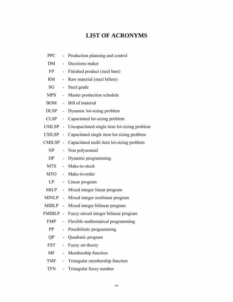
LIST OF ACRONYMS
PPC - Production planning and control
DM - Decisions maker
FP - Finished product (steel bars)
RM - Raw material (steel billets)
SG - Steel grade
MPS - Master production schedule
BOM - Bill of material
DLSP - Dynamic lot-sizing problem
CLSP - Capacitated lot-sizing problem
USILSP - Uncapacitated single item lot-sizing problem
CSILSP - Capacitated single item lot-sizing problem
CMILSP - Capacitated multi item lot-sizing problem
NP - Non polynomial
DP - Dynamic programming
MTS - Make-to-stock
MTO - Make-to-order
LP - Linear program
MILP - Mixed integer linear program
MINLP - Mixed integer nonlinear program
MIBLP - Mixed integer bilinear program
FMIBLP - Fuzzy mixed integer bilinear program
FMP - Flexible mathematical programming
PP - Possibilistic programming
QP - Quadratic program
FST - Fuzzy set theory
MF - Membership function
TMF - Triangular membership function
TFN - Triangular fuzzy number

xvi
RLT - Reformulation-linearization technique
B&B - Branch-and-bound
BD - Benders decomposition
CV - Complicating variable
NCV - Non-complicating variable
MP - Master problem
SP - Sub-problem
xvii
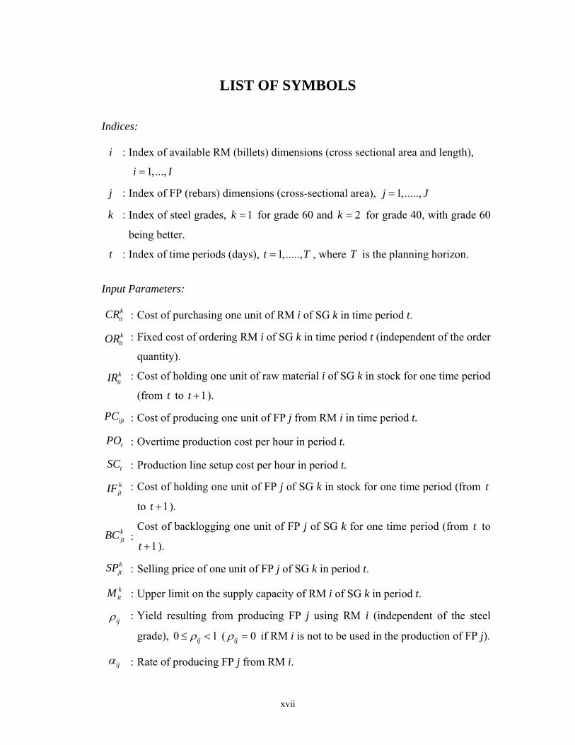
LIST OF SYMBOLS Indices:
i : Index of available RM (billets) dimensions (cross sectional area and length),
1,...,i I=
j : Index of FP (rebars) dimensions (cross-sectional area), 1,.....,j J=
k : Index of steel grades, 1k = for grade 60 and 2k = for grade 40, with grade 60
being better.
t : Index of time periods (days), 1,.....,t T= , where T is the planning horizon.
Input Parameters:
kitCR : Cost of purchasing one unit of RM i of SG k in time period t.
kitOR : Fixed cost of ordering RM i of SG k in time period t (independent of the order
quantity). kitIR : Cost of holding one unit of raw material i of SG k in stock for one time period
(from t to 1t + ).
ijtPC : Cost of producing one unit of FP j from RM i in time period t.
tPO : Overtime production cost per hour in period t.
tSC : Production line setup cost per hour in period t. kjtIF : Cost of holding one unit of FP j of SG k in stock for one time period (from t
to 1t + ).
kjtBC :
Cost of backlogging one unit of FP j of SG k for one time period (from t to
1t + ). kjtSP : Selling price of one unit of FP j of SG k in period t.
kitM : Upper limit on the supply capacity of RM i of SG k in period t.
ijρ : Yield resulting from producing FP j using RM i (independent of the steel
grade), 0 1ijρ≤ < ( 0ijρ = if RM i is not to be used in the production of FP j).
ijα : Rate of producing FP j from RM i.
xviii
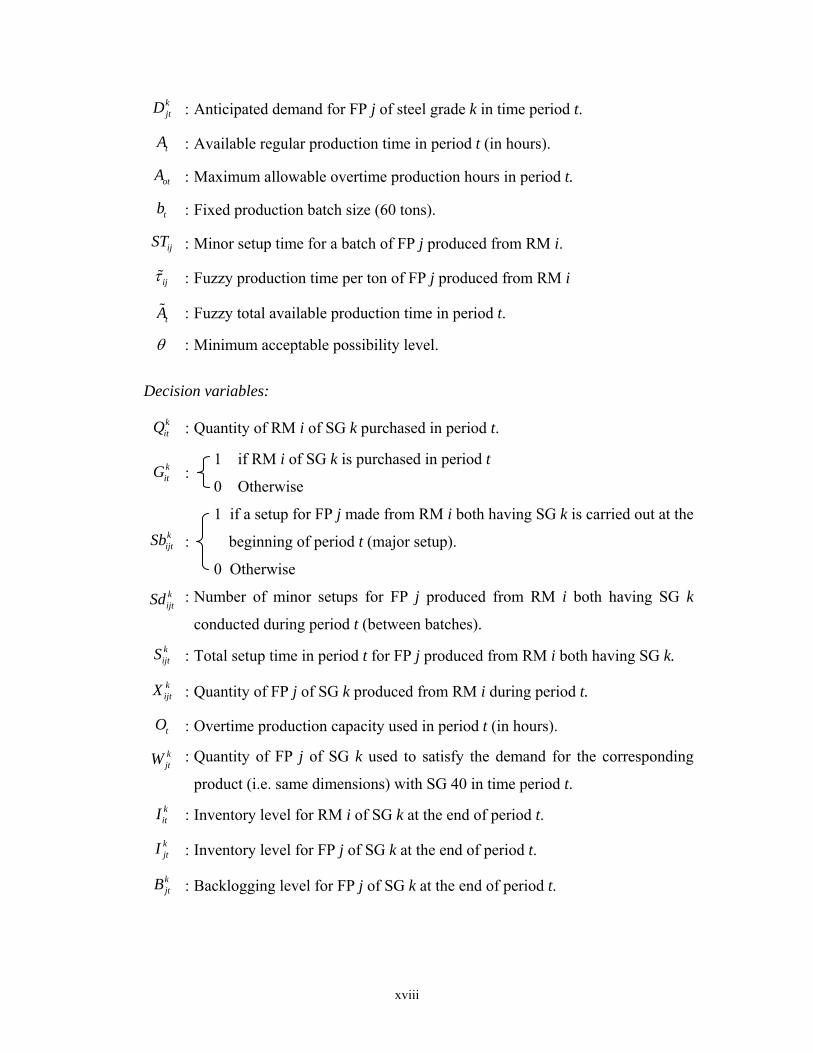
kjtD : Anticipated demand for FP j of steel grade k in time period t.
tA : Available regular production time in period t (in hours).
otA : Maximum allowable overtime production hours in period t.
tb : Fixed production batch size (60 tons).
ijST : Minor setup time for a batch of FP j produced from RM i.
ijτ : Fuzzy production time per ton of FP j produced from RM i
tA : Fuzzy total available production time in period t.
θ : Minimum acceptable possibility level.
Decision variables:
kitQ : Quantity of RM i of SG k purchased in period t.
kitG :
1 if RM i of SG k is purchased in period t
0 Otherwise
kijtSb :
1 if a setup for FP j made from RM i both having SG k is carried out at the
beginning of period t (major setup).
0 Otherwise kijtSd : Number of minor setups for FP j produced from RM i both having SG k
conducted during period t (between batches). kijtS : Total setup time in period t for FP j produced from RM i both having SG k.
kijtX : Quantity of FP j of SG k produced from RM i during period t.
tO : Overtime production capacity used in period t (in hours). kjtW : Quantity of FP j of SG k used to satisfy the demand for the corresponding
product (i.e. same dimensions) with SG 40 in time period t. kitI : Inventory level for RM i of SG k at the end of period t.
kjtI : Inventory level for FP j of SG k at the end of period t.
kjtB : Backlogging level for FP j of SG k at the end of period t.
1
Chapter 1
Introduction
1.1 Background and Motivation
The intensive competition in today’s operating environment has made it
increasingly important for industrial enterprises to continuously seek the best
practices towards managing their operations and, eventually, differentiate themselves
from their competitors. In particular, the optimization of production and inventory
related decisions provides a vital step towards a better fulfillment of customers’ needs
at a minimum cost. Such decisions determine the required machining capacity,
workforce levels, space utilization among other factors, which all combined have a
direct impact on the financial health of an organization.
Steel manufacturing, for instance, represents one of the backbone industries
greatly affecting a nation’s economic growth and pace of development. Needless to
say, a substantial portion of today’s indispensable products that are used on a daily
basis and serve multiple purposes have steel ingredient in them, in one form or
another, ranging from sophisticated high-tech products such as cars and airplanes, to
much simpler products such as kitchen utensils. Steel mills, which are the focus of
this research, produce a variety of the most essential products including steel wires,

2
pipes, bars, rods and sheets. In North America only, more than 100 million tons of
steel are produced annually with an estimated value of over 50 billion dollars (Denton
et al. 2003).
In general, the iron and steel industry is characterized by being both capital and
energy intensive and, as such, the importance of effective production planning in such
industry is by no means less than that in any other industry. For a rolling mill
producing between 300,000 and one million tons of steel annually, the capital
investment is measured in tens of millions of dollars (Denton et al. 2003). Upon
realizing the major investments associated with the construction and operations of
steel plants, the main concern of steel manufacturers has been the adoption of the
latest technology advances in the production process as well as finding better ways to
manage the rapid increase in product variety. However, in spite of the significance of
steel industry, planning and scheduling problems in iron and steel production have
not drawn as wide attention of the production and operations management research
community as many other industries such as metal cutting and electronics industry
(Tang et al. 2001). The work presented in this thesis targets this deficiency and
bridges the gap between theory and practice through dealing with a realistic case
study encountered in steel rolling mills. From a theoretical standpoint, the production
planning problem addressed in this thesis falls under the broad class of the well
known dynamic lot-sizing problem (DLSP). However, several practical extensions
are incorporated in order to account for the technological constraints associated with
the manufacturing process. Hence, it is important to step back and establish the

3
theoretical background behind the basic DLSP and shed some light on some of its
distinguishing characteristics.
1.2 A closer look at the dynamic lot-sizing problem
Typically, this class of problems refers to medium term planning decisions in
which the production mix and quantities are usually planned ahead on a weekly or a
monthly basis. The planning horizon is divided into a number of discrete time
intervals of equal length, each having its own demand, hence the term dynamic. In a
manufacturing firm context, a lot refers to the items produced consecutively, one after
the other, on the same machine, production line, or facility since the last setup. The
lot size is simply the number of items contained in a particular lot. Hence, lot-sizing
is the activity to obtain simultaneously in which period, and in which number (i.e. lot
size) different items should be produced such that the production plan is feasible. In
general, making the right decisions in lot-sizing will affect directly the system
performance and its productivity, which are important for a manufacturing firm’s
ability to compete in the market (Karimi et al. 2003).
However, a clear distinction has to be made between two different types of the
LSPs. First, the continuous time scale, constant demand and infinite time scale lot
sizing problems. The credit of initiating the work related to this problem goes to
Harris (1913) where he introduced the widely used nowadays economic order
quantity (EOQ) model. The basic economic manufacturing quantity (EMQ) model
and the economic lot scheduling problem (ELSP) also fall under this category. The
other class deals with the discrete time scale, dynamic demand and finite time horizon
problems, usually referred to as the dynamic lot sizing problem (DLSP). Typically,
4
the latter case involves the development of a mathematical model that seeks the
minimum setup cost, production cost and inventory holding cost. In reality, these
costs differ from one item to another depending on the complexity and size of the
item. Other types of costs include backorder, lost sales, outsourcing and rework cost
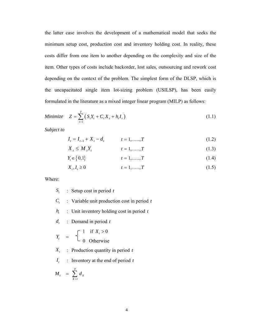
depending on the context of the problem. The simplest form of the DLSP, which is
the uncapacitated single item lot-sizing problem (USILSP), has been easily
formulated in the literature as a mixed integer linear program (MILP) as follows:
Minimize ( )1
T
t t t t t tt
Z S Y C X h I=
= + +∑ (1.1)
Subject to
1t t t tI I X d−= + − 1, .....,t T= (1.2)
t t tX M Y≤ 1, .....,t T= (1.3)
{ }0,1tY ∈ 1, .....,t T= (1.4)
, 0t tX I ≥ 1, .....,t T= (1.5)
Where:
tS : Setup cost in period t
tC : Variable unit production cost in period t
th : Unit inventory holding cost in period t
td : Demand in period t
tY = 1 if 0tX >
0 Otherwise
tX : Production quantity in period t
tI : Inventory at the end of period t
tM = T
kk t
d=∑

5
The objective is to minimize the total cost composed of setup, production and
inventory holding costs. Constraints (1.2) represent the inventory balance equations,
and constraints (1.3) are the fixed charge constraints which establish the relation
between the binary variable tY and the continuous variable tX , and also set an upper
bound on the production quantity per period.
1.3 Characteristics of the dynamic lot-sizing models
The DLSP covers a wide spectrum of production planning problems encountered
in several industrial applications. Depending on the features of each, the DLSPs range
from simple ones, which can be solved to optimality with exact algorithms such as
the USILSP, to much more complicated ones (NP-complete) for which no optimal
solution exists and a heuristic solution is adopted. Figure 1.1 provides a classification
of the DLSPs based on the characteristics distinguishing them from one another. The
figure combines and extends the work of Karimi et al. (2003) and Haase (1994).
Figure 1.1: Characteristics of the dynamic lot-sizing problem
Lot-sizing problems
Planning horizon Big bucket vs. small buckets
Number of levels Single-level vs.
multi-level
Number of products Single-item vs.
multi-item
Capacity restrictionUncapacitated vs.
capacitated
Nature of the product
Demand Pattern - Static vs. dynamic
- Deterministic, probabilistic or fuzzy
Setup structure Simple vs. complex
Service policy Backlogging vs. lost
sales
6
1.3.1 Planning Horizon
The planning horizon for the DLSP is usually finite and it might be quite short
that only one item can be produced in that period, or long enough to accommodate the
production of several items within the same period. In the latter case, the problem is
called big bucket where this differs from the small bucket, the first case, in the fact
that it also considers the sequence of the production lots, which gives rise to the well
known lot sizing and scheduling problem. In the literature, lot sizing and scheduling
decisions are usually treated independently for simplifying the overall decision
making problem (Ozdamar et al. 1998).
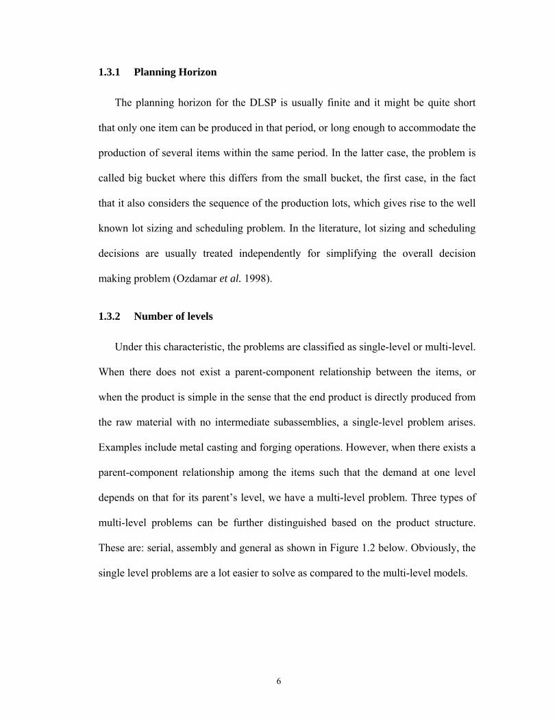
1.3.2 Number of levels
Under this characteristic, the problems are classified as single-level or multi-level.
When there does not exist a parent-component relationship between the items, or
when the product is simple in the sense that the end product is directly produced from
the raw material with no intermediate subassemblies, a single-level problem arises.
Examples include metal casting and forging operations. However, when there exists a
parent-component relationship among the items such that the demand at one level
depends on that for its parent’s level, we have a multi-level problem. Three types of
multi-level problems can be further distinguished based on the product structure.
These are: serial, assembly and general as shown in Figure 1.2 below. Obviously, the
single level problems are a lot easier to solve as compared to the multi-level models.

7
Figure 1.2: Various product structures 1.3.3 Number of products
The number of end items accounted for in a lot-sizing model greatly affects the
complexity of the problem. If there is only one end item (final product) to plan for,
then a single-item problem arises. On the contrary, if planning is carried out for
multiple end items, the problem becomes more involved and it is a multi-item
planning problem.
1.3.4 Resource constraints In practice, a resource might refer to a machine capacity, storage space, available
budget or manpower. Once abundant amount of resources exist, the problem is coined
as “uncapacitated”. When there exist a restriction on one of the resources, e.g.,
production capacity, which resembles most practical real life systems, the problem is
“capacitated” which adds another dimension of complexity to the model.
1.3.5 Nature of the product
The nature of the end items also affects the production strategy, as perishable
items shall not be produced way ahead of the time they are actually needed since they
Serial Assembly General Level
Final item 1
2
3
4

8
might become obsolete while still in stock. The diary products set a good example for
such items. Conversely, automobiles, for instance, represent those items which
deteriorate over time reducing their value once sold after being in stock for a long
time. Non-deteriorating items, those maintaining their value regardless of the storage
period, are easier to deal with as it might be more economical to produce them ahead
of time in periods of excess capacity.
1.3.6 Demand Pattern
The firm might be facing a static demand over time, or one that changes from a
time period to another (dynamic demand). Viewing it from a different perspective, if
the demand is known with a high degree of certainty, then it is called “deterministic”.
However, obtaining an exact value of the market demand might not be easily
achievable or even not at all in case of a highly volatile demand, which necessitates
the use of probability distributions to represent the “stochastic demand”. Another
pattern that is commonly overlooked by researchers is dealing with the demand as a
fuzzy quantity. That is, instead of assigning it a single crisp value, the demand is
represented by a set that spans over a certain range, with a likelihood value specifying
the degree of compatibility of each element with the set. The range and the
compatibility (membership value) for each element is decided upon through
experience and human subjective judgment, as explained in Section 1.4.
1.3.7 Setup structure
Typically, whenever the manufacturing process is switched from producing one
product to another, a setup activity is incurred, which entails a setup time as well as

9
an associated setup cost. A clear exception is the labor based operations where
machinery is not involved such as some assembly processes. While a simple setup is
the one independent of the products sequence, a setup activity that depends on the
sequence of the products gives rise to a more complicated problem, which can be
modeled as the famous traveling salesman problem (TSP).
1.3.8 Service policy
The inventory levels maintained by the firm depend on its policy when it comes to
demand fulfillment. Backlogging occurs when the demand of the current period
cannot be satisfied on time and is thus satisfied in future periods. On the other end, a
demand that is not satisfied momentarily in the same period with no chance of
fulfilling it afterwards is lost and hence the title “lost sales”. The options of
outsourcing or working overtime could also be utilized to handle the excess demand.
At this juncture, it is important to establish the equivalence between the master
production scheduling (MPS) problem and a specific class of DLSP. Both MPS and
the big-bucket, multiple-item, single-level DLSP establish the production quantities
for the final product in each period. The inventory management literature usually
coins the term DLSP to refer to this class of problems while the production planning
researchers mostly coin the MPS term. In this thesis, the production planning problem
is tackled at the MPS level and hence the two terms are used interchangeably.
1.4 Fuzzy set theory as applied to the lot-sizing problem
In reality, firms operate in a rapidly changing and constantly evolving
environment, where several external factors such as market, technology, etc., play an

10
important role. As a result, the certainty assumption imposed in most lot-sizing
models is often unsatisfied as the estimation of model parameters is based on the
prediction of future events. Whenever there is a high level of ambiguity involved, the
Fuzzy set theory (FST) approach stands out as the favorable one. In the second and
third parts of this thesis, we make use of the FST to account for the uncertainties
associated with customer demand and production capacity. The suitability of
choosing the fuzzy tool to represent these quantities is briefly discussed below.
1.4.1 Fuzzy demand
When dealing with a make-to-stock (MTS) environment, the decisions made in a
typical lot-sizing problem are of medium range planning horizon, which have a
typical time frame ranging from a week to several months. Since the main goal of a
lot-sizing model is to optimally decide on the production quantities and timings for a
certain number of time periods in the future, lots of uncertainties are involved due to
the continuously evolving nature of the environment in which a firm operates which
makes the forecasts for future customer demand less reliable. With the multi-item
case, the uncertainty is even more obvious in the sense that it might be associated
with the volume or the mix. This uncertainty that is associated with future demand
can be specified based on experts’ opinion and managerial subjective judgment.
Possible representation for an uncertain demand using fuzzy sets is as follows:
(a) Demand is around md , but definitely not less than ld and not greater than ud .
This is represented by a triangular fuzzy number.

11
(b) Demand definitely falls in the interval [ ],l ud d with a high degree of possibility
to fall in the smaller interval [ ],lm umd d . This is called a trapezoidal fuzzy
number.
(c) Demand is much larger than ld , represented by a linear membership function.
(d) Demand is much smaller than ud , represented by a linear membership function.
The above natural language expressions can be represented as fuzzy sets with the
possibility distributions shown in Figure 1.3.
Figure 1.3: Alternative fuzzy sets to represent fuzzy demand
dl du dlm D
Dμ
dum dl dudm D
Dμ
1
0 0
1
dl du D
Dμ
1
0 dl du D
Dμ
1
0
(a) (b)
(c) (d)

12
A membership function of fuzzy customer demand can be derived either from
subjective manager belief or from its probability distribution if it exists (Dubois and
Prade 1994). However, it is important to note that possibility distribution differs from
the probability distribution both in principle and in practice. Petrovic et al. (1999)
demonstrate the suitability of using fuzzy sets to describe customer demand through
an example:
“Consider customer demand as in Figure 1.3 (b). Suppose that circumstances have
brought into existence a strong belief that customer demand can be 2+ ud with
possibility 1. In such a case, it is easy to modify the existing possibility distribution by
simply adding a new possible value of demand with no other changes of the
distribution. Let us notice that such an intervention, having a probability distribution,
is not straightforward at all”.
In some practical situations, the demand pattern can be adequately modeled with
deterministic or probabilistic values. However, in other situations, the validity of such
representation is highly questionable. Examples include:
1. A company entering a new market sector and aiming towards building a chain of
new customers.
2. The product is newly introduced to the market, and the company has no clue of
what the future demand pattern would look like.
3. In the absence of reliable historical data of the demand that are representative of
the future demand, or when these data are not a trusted source any more due to a
change in the operating environment or other factors (the global financial crisis
that took place in 2008-2009 sets a good example for this case).
13
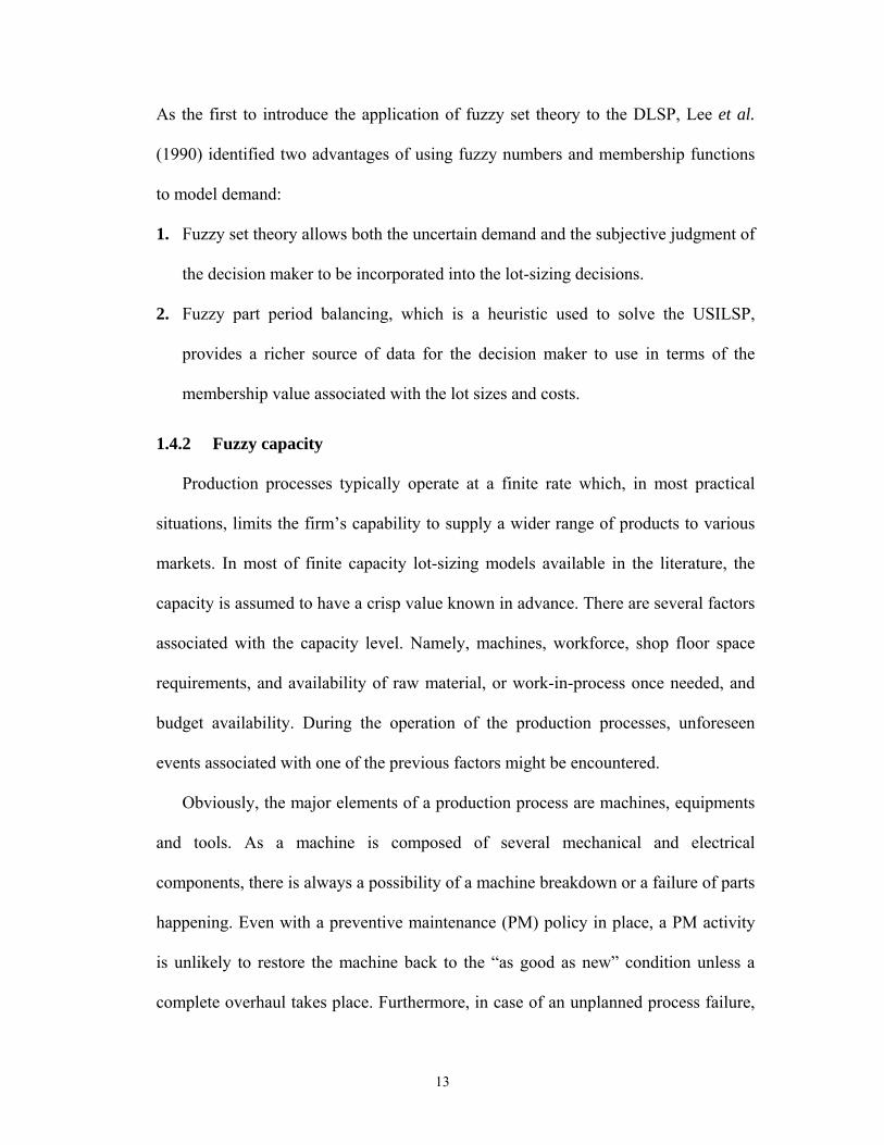
As the first to introduce the application of fuzzy set theory to the DLSP, Lee et al.
(1990) identified two advantages of using fuzzy numbers and membership functions
to model demand:
1. Fuzzy set theory allows both the uncertain demand and the subjective judgment of
the decision maker to be incorporated into the lot-sizing decisions.
2. Fuzzy part period balancing, which is a heuristic used to solve the USILSP,
provides a richer source of data for the decision maker to use in terms of the
membership value associated with the lot sizes and costs.
1.4.2 Fuzzy capacity
Production processes typically operate at a finite rate which, in most practical
situations, limits the firm’s capability to supply a wider range of products to various
markets. In most of finite capacity lot-sizing models available in the literature, the
capacity is assumed to have a crisp value known in advance. There are several factors
associated with the capacity level. Namely, machines, workforce, shop floor space
requirements, and availability of raw material, or work-in-process once needed, and
budget availability. During the operation of the production processes, unforeseen
events associated with one of the previous factors might be encountered.
Obviously, the major elements of a production process are machines, equipments
and tools. As a machine is composed of several mechanical and electrical
components, there is always a possibility of a machine breakdown or a failure of parts
happening. Even with a preventive maintenance (PM) policy in place, a PM activity
is unlikely to restore the machine back to the “as good as new” condition unless a
complete overhaul takes place. Furthermore, in case of an unplanned process failure,

14
the duration of a corrective maintenance (CM) action aimed at restoring the process
to the operational status depends on the parts to be fixed or replaced and on the
availability of spare parts, as needed. Another incident frequently encountered is the
production of faulty or defective items. Such items consume partial capacity, during
production, with no actual contribution to the output delivered to the customer. In
addition, there is a setup activity associated with switching production from one item
to another, and the duration of this setup may vary between workers depending on
experience. A setup delay can happen or, conversely, a setup might be accomplished
faster than usual due to a skilled worker performing it.
Even when machine’s availability turns out to be precisely as expected, the
workers responsible for operating those machines add another dimension of
uncertainty to the capacity. Workers absenteeism or on-job injuries due to a
hazardous working environment, which is the case for steel mills, could cause the
machine to be idle for some time unless a substitute worker is readily available. With
no obstacles concerning machines, labor or space, the production process might still
starve due to late deliveries of work-in-process from the previous production process,
or a late arrival of a shipment of raw material from an external supplier.
The need to deal with capacity as a vague and imprecise quantity rather than
assigning it a single crisp value stems from the uncertainties associated with the
above mentioned factors affecting capacity. Unplanned machine breakdown, faulty
production, workers injury, space limitation and electricity outage, all result in a
production time capacity being less than what is planned for. On the other hand,
working extra shifts or overtime, and workers operating more efficiently contribute to

15
a capacity larger than what was thought of. Hence, the assumption of constant
capacity is clearly an oversimplified version of the situations encountered in practice,
where the above factors are completely ignored. A better approach would be to
represent the capacity with a fuzzy set, triangular or trapezoidal as shown in parts (a)
and (b) of Figure 1.3 respectively. The most likely value(s) would represent the
expected available capacity based on experience, intuition and subjective human
judgment. The left-most and the right-most values represent the most pessimistic and
the most optimistic capacity levels, respectively.
1.5 Research Objectives
Effective production planning at steel rolling mills bares a great importance and
plays a major role towards reducing the high costs associated with constructing and
operating steel plants. Moreover, there are some distinguishing features of the steel
rolling process that sets it apart from the other industries and that needs to be taken
into consideration in order for the developed production plans to be implementable.
These features include complex setup time structure, batch manufacturing, scrap and
production rates that depend on the input and output material, overtime, allowed
backlogging and one-way substitutability of the end-items.
Our objective in the first phase of this research is to develop an optimized master
production schedule (MPS) that considers the above interrelated factors under static
demand conditions. Studying these factors under static conditions shall provide
greater insights on the combined effect they have on the production planning
decisions and the tradeoffs amongst them. As the problem involves multiple inputs
and multiple outputs (i.e., both are available in different sizes and grades as explained
16
later in Chapter 3), the objective is not only to optimize the production and inventory
of the end-items, but also to establish the input-output combinations and accordingly
the raw material (i.e., input) procurement and inventory policy. It is also the objective
of this phase to define and develop a unified framework for the existing solution
methodologies capable of handling the proposed mathematical model. We seek to
study several alternative solution algorithms with varying performance capabilities in
terms of efficiency and quality of solutions obtained.
The second phase of this research is geared towards optimizing the production
and inventory related decisions while taking into account the dynamic nature of the
operating environment. This dynamicity is mainly attributed to highly changing
customers’ preferences coupled with their heightened expectations of shortened
delivery lead times. Under these conditions of demand volatility, the development of
an optimized MPS turns out to be a challenging task. Hence, to achieve the stated
objective, we need to develop efficient mathematical models that capture the frequent
changes in the problem parameters and quickly react to these changes on a rolling
horizon basis.
The rigidity requirement of classical mathematical programming techniques is
overcome through the use of FST which allows for uncertainties in demand to be
taken into account. The second face of this research also aims at establishing the
benefits obtained via adopting fuzzy mathematical programming techniques as
opposed to the use of its crisp counterpart. We emphasize on establishing the missing
distinction in the literature between the two approaches typically adopted to handle
fuzziness within mathematical programming models, namely flexible mathematical

17
programming (FMP) and possibilistic programming (PP). In the context of FMP,
aggregation operators are used to combine the fuzzy sets defining the objective
function and the constraints in order to obtain the fuzzy decision set. This research
shall utilize two different operators, one of which is compensatory while the other is
not, in an attempt to evaluate the benefits obtained via each operator in terms of
savings in the total costs incurred.
In the last part of this research, the goal is to incorporate both internal as well as
external sources of uncertainty associated with production capacity and customers’
demand into the planning decisions. Hence, we need to investigate how various
sources of uncertainty can be represented differently and incorporated simultaneously
within the same mathematical model through the combined utilization of FMP and PP
approaches. Since the decision maker specifies the minimum acceptable possibility
level, it is also the objective of this analysis to study the effect of varying the
possibility levels on the planning decisions, and the total cost incurred. .
1.6 Research Methodology
An outline of the adopted research methodology to tackle the production planning
problem at hand is given in Figure 1.4. After conducting several visits to the plant and
identifying a realistic problem encountered frequently in steel rolling mills, a
literature review is carried out and the relevant theoretical basis for such problem is
established. Then, the necessary data is acquired and the problem is formally defined
along with the stipulated assumptions and the distinguishing characteristic of this
industry. The technique of mathematical programming is employed in order to
optimize the operations at the steel mill under static conditions through the

18
construction of a mathematical model that incorporates the technological constraints
associated with the manufacturing process. The solution to the proposed model is
obtained through several solution algorithms; namely the classical linearization
approach, a hybrid linearization-Benders decomposition approach and a modified
branch-and-bound algorithm, where all these algorithms were coded in AMPL
programming language and solved using CPLEX 11.0 solver. To account for demand
uncertainties, the original model is first applied on a rolling horizon basis where the
decisions concerning the most immediate time period only are implemented before
rolling the horizon forward and updating the problem parameters. This requires the
repetitive solution of the exact model and hence viable approximations that target the
complicating aspects of the exact model are developed. The alternative approach to
deal with demand uncertainty is the use of FST where the material balance constraints
are treated as flexible/soft constraints. The resulting fuzzy model is non-symmetric
which calls for the fuzzification of the objective function first. The linearization
approach coupled with exterior penalty function methods (EPFM) is adopted in order
to identify the interval of allowance on the decision maker’s (DM) aspiration level.
The aggregation of the fuzzy sets representing the DM aspiration level as well as the
constraints is accomplished using two different aggregation operators which results in
two variants of the approximate auxiliary models. In the last phase, both uncertain
demand and production capacity are accounted for in a fuzzy model where the
concepts of FMP and PP are jointly employed. In addition, we utilize the weighted
average method in order to deal with triangular fuzzy numbers and the fuzzy ranking
method in order to deal with constraints involving fuzzy quantities on both sides. To

19
Figure 1.4: Research methodology
Identifying a realistic case study from the steel
rolling industry
Literature review and establishing the
theoretical background
Data acquisition and formal definition of the
problem
Mathematical model formulation for
deterministic conditions
Develop solution algorithms and test their
performance
Extending the model to handle dynamic
operating conditions
Account for demand uncertainty through
FMP
Account simultaneously for uncertain demand and capacity via FMP and PP
Account for demand uncertainty through
rolling horizon schedules
Fuzzification of the objective function
Develop approximate models that generate exact schedules only
Solve the approximate models directly or via
linearization first
Solve the approximate auxiliary models for two
aggregation operators
Solve the approximate auxiliary models for two
aggregation operators
Models testing and validation for several
problem instances
Model testing and validation for several
problem instances
Model testing and validation for several
problem instances
Fuzzification of the objective function
20
serve testing and validation purposes for the developed models, several problem
instances with different degrees of complexity are prepared. The values of the input
parameters are generated from realistic data ranges so that the practicality of the
developed models and solution algorithms is ensured.
1.7 Thesis outline
The remainder of this thesis is organized as follows. Chapter 2 reviews the
literature for the general DLSP, in its basic and extended forms, and the more relevant
production planning practices in the steel rolling industry. In Chapter 3, a formal
definition of the problem is given along with a mathematical formulation that
addresses the various aspects of the operating environment and the manufacturing
process. This initial model assumes the availability of highly reliable demand
forecasts and relatively accurate capacity estimates. Hence, it seeks to provide some
insights into the impact of several interrelated factors on the planning decisions under
stable operating conditions. As the developed model is a mixed integer bilinear
program (MIBLP), the theoretical background for those solution methodologies that
can be directly applied or specifically modified to solve this class of models is
provided in the appendix. The application/customization of these algorithms to the
model at hand is detailed in Chapter 4 and also their performance is benchmarked
against one another for several problem instances.
The second part of the research takes the problem one step closer to reality
through incorporating uncertainties associated with end customer demand in the
planning process. Chapter 5 addresses these uncertainties through the inclusion of
21
both the forecasted demand and the confirmed customers’ orders and then applying
the resulting model on a rolling horizon basis, where production in the most
immediate time period is established based on the confirmed orders. Due to the
substantial computation time required to solve the exact model at the beginning of
each period, approximate models that result in a tractable number of binary and/or
integer variables are developed and tested. In Chapter 6, the alternative approach of
utilizing FST, which allows for the incorporation of the decision maker’s preference
modeling, is presented. A brief background is first established followed by a clear
distinction between the FMP and PP, which represent the commonly used concepts to
handle existent fuzziness in mathematical programs. The “min operator” and the
“convex combination of the min and max operators” are used to aggregate the fuzzy
sets representing the objective function and the constraints. The resulting auxiliary
models are solved under different settings of the problem parameters in an attempt to
quantify the benefits obtained form using the fuzzy models instead of the crisp ones.
In the last part of this research, Chapter 7 addresses jointly the uncertainties
associated with the demand and the production capacity in the same model. The
importance of this model is to illustrate how different uncertainty sources can be
expressed through combining the concepts of FMP and PP in one mathematical
model. The utilization of the weighted average method and the fuzzy ranking
technique shall be of particular interest to future researchers. A summary of the
research work, concluding remarks and suggestions for future research directions are
stated in Chapter 8.

22
Chapter 2
Literature Review
2.1 Introduction
The production planning problem addressed in this thesis can be viewed as an
instance of the well know dynamic lot-sizing problem (DLSP) with several
extensions that are needed to account for the actual practice. As shall be explained in
Chapter 3, the steel rolling process has a continuous flowshop layout and, as far as
this work is concerned, can thus be dealt with as a single stage Lot-sizing problem
(LSP). Undoubtedly, this class of LSPs is simpler to handle as opposed to the multi-
stage version, since the latter involves deciding upon the production or purchasing lot
sizes for several items constituting a product’s bill-of-material (BOM). Hence, the
work reviewed in this chapter focuses on the single stage DLS models as these are
more relevant to the production planning problem at hand. The literature review
presented in this chapter is divided into two main sections. The first discusses the
work related to the LSP in the general context, in its basic and extended forms, while
the second considers the more related work addressing production planning problems
as applied to the steel industry. As we introduce some of the concepts and solution

23
methodologies utilized in this research, the relevant literature will be reviewed in the
respective chapters.
2.2 Single Stage Dynamic Lot-Sizing Problem
Due to its wide spread applications in various industries, the DLSP has received a
great deal of interest from industrial practitioners as well as academic researchers.
Since the introduction of this problem through the famous work of Wagner-Whitin
(1958) and Manne (1958), there have been numerous amounts of research addressing
the DLSP in different sittings and under various assumptions. The state-of-the-art
advances in the DLSP could be found in De Bodt et al. (1984), Bahl et al. (1987),
Maes and Van Wassenhove (1988), Wolsey (1995), Drexl and Kimms (1997), Karimi
et al. (2003), Brahimi et al. (2006), Jans and Degraeve (2007, 2008) and Quadt and
Kuhn (2008). However, as reported by Karimi et al. (2003): “There has been little
literature regarding problems such as capacitated lot sizing problems (CLSP) with
backlogging or with setup times and setup carry-over”. The review of this section is
divided into subsections, each considering the work related to an issue that is
addressed in the thesis.
2.2.1 Basic lot-sizing models
Maes and Van Wassenhove (1986a) points out that capacitated lot sizing models
are powerful and very flexible but slow (or impossible) to solve if the problem
instance is very large. In terms of complexity theory, the capacitated single item lot-
sizing problem (CSILSP) is NP-hard in general. It is even NP-hard for very special

24
cases (Bitran and Yanasse 1982). However, Chen et al. (1994) proved through a
pseudo-polynomial dynamic programming algorithm that the CSILSP is not NP-hard
in the strong sense.
Since it was first introduced, the DLSP has seen many contributions, some of
which were from a modeling perspective through providing tighter formulations of
the problem, while others developed solution algorithms that outperform the already
existing ones in either the solution time or the quality of the solutions obtained or
even both. This section intends to highlight the advances made in the basic DLSP (i.e.
with no extensions).
Wagner and Whitin (1958) and Manne (1958) started a whole new research
direction in their seminal papers. Wagner-Whitin (WW) proved that there exists an
optimal solution to the uncapacitated SILSP in which production never takes place in
a period while having inventory left from the previous period. This property implies
that production in one period, if any, should satisfy the demand for an integral
number of consecutive periods. Based on this property, they developed a dynamic
programming (DP) algorithm of 2( )O m , with m being the number of time periods.
The complexity of the DP algorithm for the uncapacitated SILSP was independently
reduced from 2( )O T for the case of WW to (O T log )T by several authors including
Federgruen and Tzur (1991), Wagelmans et al. (1992) and Aggarwal and Park
(1993). Manne (1958) proposed an innovative formulation for the capacitated version
of the problem with setup times incorporated. He explicitly models all the possible
schedules with different setup sequences. Evans (1985) proposed a shortest path
formulation for the USILSP based on a graph representation of the problem. As the
25
reformulations provide improved lower bounds on the optimal solution value, their
LP solution can also be used to construct heuristic solutions. Belvaux and Wolsey
(2001) explain how many extensions of the basic lot sizing models can be modeled in
order to obtain better formulations. A recent survey of the modeling techniques as
applied to the LSPs is given by Jans and Degraeve (2008).
From a solution methodology perspective, there exists several heuristics that are
dedicated for solving the USILSP. Those heuristics are usually easier to implement
than the WW algorithm. Examples include economic order quantity based on average
demand, least period cost (Silver and Meal 1973), least unit cost, part-period
balancing among many others. A discussion of such heuristics can be found in Silver
et al. (1998). Moreover, Bitran et al. (1984), Axsäter (1985) and Coleman (1992)
studied the performance of some of these heuristics and developed worst-case bounds
under several demand classes. A dynamic programming based algorithm for the
USILSP was developed By Kirca (1990). First, the algorithm generates the set of all
feasible cumulative production levels that may occur in an optimal solution, and then
a DP procedure is carried out over this set. Diaby (1993) developed an efficient post-
optimization procedure that re-computes the optimal schedule starting from the WW
solution for the case where some set ups are imposed or prohibited. Chung et al.
(1994) constructed a hybrid algorithm combining both DP and branch and bound
towards solving the same problem.
On the other hand, the CMILSP has received remarkable attention as it is a more
challenging problem to solve. Several exact solution methods have been proposed.
Barany et al. (1984) and Pochet and Wolsey (1991) used valid inequalities (strong

26
cutting planes) to solve the problem. Eppen and Martin (1987) established a shortest
path formulation of the DP recursion presented in WW, where this network
formulation sets a tighter lower bound for the problem. Constantino (1998) also
derived families of strong valid inequalities and showed that they are sufficient to
completely describe the convex hulls of the sets of feasible solutions. Belvaux and
Wolsey (2000) developed an efficient branch-and-cut based software that includes
preprocessing and cutting planes for a variety of lot sizing models.
Apart from the exact methods, there are some heuristics that have been
specifically tailored for solving the CMILSP. Dixon and Silver (1981) extended the
Silver-Meal heuristic to the capacitated multi item case. The criterion is to select that
item for which a one period increase in the supply results in the largest decrease in
average cost per unit time per unit of capacity absorbed (Jans and Degraeve 2007).
Dogmaraci et al. (1981) developed a forward sweep algorithm along with a greedy
search starting from the lot-for-lot solution. Karni and Roll (1982) use the WW
schedules as a starting point and try to achieve feasibility while optimizing cost
through shifting production. Maes and Van Wassenhove (1986c) implemented several
cost criteria in their ABC heuristic to determine whether or not to include next
period’s demand, and several other rules to determine the order of the items. Finally,
Kirka and Kökten (1994) developed an efficient item-by-item heuristic where items
are selected one at a time, and then a single item problem is solved with adapted
capacities and extra bounds on production and inventory to ensure the feasibility of
the overall problem.

27
Another approach towards solving the CMILSP is the use of Lagrangian
relaxation, e.g., Thizy and Van Wasenhove (1985), Trigerio et al. (1989) and Diaby
et al. (1992). The traditional practice in this approach is to get rid of the complicating
capacity constraint through a dualized term in the objective function coupled with a
specific set of positive multipliers. The resulting problem is a lot easier to solve and
may be decomposed into separate single item uncapacitated subproblems for each
item.
Polynomial approximation technique has also been applied towards solving the
LSPs. Bitran and Matsuo (1986) proposed a pseudo-polynomial approximation
algorithm for the CMILSP based on Manne’s (1958) formulation. Gavish and
Johnson (1990) developed a fully polynomial approximation scheme for the
capacitated single item lot scheduling problem. Furthermore, Van Hoesel and
Wagelmans (2001) presented a fully polynomial algorithm for the CSILSP, which
produces solutions with a relative deviation from the optimality that is bounded by a
constant.
Meta-heuristics such as Tabu search (e.g. Hindi 1996) and Genetic algorithms
(e.g. Gutierrez et al. 2001) have also been specifically developed to solve the
CMILSP. It is interesting to note that no implementation of meta-heuristics for
solving the CSILSP can be found, as concluded by Brahimi et al. (2006) in their
review paper. On the other hand, Cattrysse et al. (1990) discussed the set-partitioning
formulation of the CMILSP and used heuristics to convert the possibly fractional
solution from the column generation step to a feasible integer one. In a different
heuristic, Hindi (1995) implemented the branch and bound method as a solution

28
strategy for the CMILSP. Chen and Thizy (1990) gave a comprehensive analysis of
relaxation methods for the problem and showed it to be strongly NP-hard. A
comparison of the performance of several solution heuristics can be found in Maes
and Van Wassenhove (1986b).
2.2.2 Lot sizing models with Extensions
The numerous extensions of the basic lot sizing problem discussed in the
literature demonstrate its flexibility to model a variety of industrial problems. Each of
the following subsections presents the advances made towards modeling as well as
solving an extended version of the basic LSP.
2.2.2.1 Lot sizing models with allowed stockouts
In practice, the capacity is typically finite and bounded by several factor such as
machines, workers, availability of raw material and storage areas among many others.
In such situations, a manufacturer might not be capable of completely fulfilling a
certain period’s demand on time due to insufficient capacity. There are two strategies
to deal with the remaining portion of demand or the “unmet demand”. First, it might
be lost in the sense that a competitor will be the one satisfying this portion of demand.
This explains the situation where we have “lost sales”, a phenomenon that usually
takes place in the retailing industry. There is a certain attached cost resulting from
revenue loss, or penalty cost due to loss of customer goodwill. Secondly, the unmet
demand can be satisfied at a later period of time. If the whole demand is satisfied late,
this is referred to as “complete backlogging” (the words backlogging and
backordering can be used interchangeably). In the case of late fulfillment of only a

29
portion of the demand, “partial backlogging” takes place. From a mathematical
perspective, permitting backlogging means that inventory levels can be negative. In
the steel industry, most customers are long term customers, and the manufacturer
might make use of his power alongside customer’s loyalty to backlog a portion of the
demand at a certain additional cost, called “backlogging cost”.
Both cases have been addressed in the literature, with the lost sales situation being
dealt with to a lesser extent. Sandbothe and Thompson (1990) proposed a necessary
condition for an optimal solution and obtained an 3( )O T algorithm when production
capacity is constant, and an (2 )TO algorithm for the case of time-varying production
capacity. In a 1993 paper, they extended their work through imposing restrictions on
both production and inventory capacities, and obtained an algorithm with the (2 )TO
time complexity. Aksen et al. (2003) introduced a profit maximization model for the
USILSP with lost sales, where costs and selling prices were assumed to be time-
variant. They showed that losing demand in spite of a nonzero inventory at hand can
sometimes be more profitable if costs or prices vary. Liu et al. (2004) developed a
strongly polynomial algorithm for the lost sales case with bounded inventory, non-
increasing setup cost, and time varying production, inventory holding and lost sales
costs. Liu and Tu (2008) studied the CSILSP with limited inventory capacity and
time-varying functions of demands and costs.
One of the earliest works to consider backlogging is due to Zangwill (1966a),
where he proposed a deterministic single-item multi-period production and inventory
model having concave production cost and piecewise concave inventory costs. The
inventory can be backlogged to a maximum of α periods, where α is called the

30
backlog limit. Zangwill (1966b) extended his previous work to the multi-product
multi-facility case with facilities being in series or in parallel, under the same cost
structure. Love (1973) was the first to present an 3( )O T DP algorithm with constant
inventory capacity, concave production and holding costs. Swoveland (1975)
developed a solution algorithm for the case of a piecewise concave production and
holding costs or backlogging costs. Moreover, Gupta and Brennan (1992) introduced
an easy and robust alternative to the WW backorder algorithm, proposed by Webster
(1989). Federgruen and Tzur (1993) proposed a simple (O n log )n solution algorithm
for the CSILSP with backlogging. Miller and Yang (1994) employed lagrangian
decomposition and lagrangian relaxation to exploit the underlying network structure
of the CMILSP with backlogging. The alternative plant location and shortest path
reformulations for the ULSP with backlogging were presented by Pocuhet and
Wolsey (1988). Recently, Chu and Chu (2007) developed a polynomial algorithm for
the CSILSP with bounded inventory and backlogging or outsourcing.
2.2.2.2 Lot sizing models incorporating setup times and/or overtime
In most practical situations, a setup is incurred whenever the manufacturing
process switches between two different products. This setup consumes partial
capacity and hence it needs to be explicitly accounted for in the mathematical model.
The Silver-Meal lot sizing heuristic for single item problems was extended to the case
of regular and overtime production capacities by Dixon et al. (1983). Also, Özdamar
and Bozyel (2000) extended the latter work to the case of CMILSP with overtime
decisions, and presented several meta-heuristics to solve the problem. Starting from
31
an initial lot-for-lot approach, Trigeiro (1989) developed a heuristic algorithm for the
CLSP with setup times that is also based on the Silver-Meal heuristic. Trigeiro et al.
(1989) and Hindi et al. (2003) considered the CMILSP with setup times and obtained
a lower bound on the value of the objective function by Lagrangian relaxation with
subgradient optimization. The polyhedral structure and valid inequalities of the single
period relaxation for the CMILSP with setup times are also presented in Miller
(2003a,b). Jans and Degraeve (2004) start with the network formulation to come up
with improved lower bounds for the problem. In a recent paper, Absi and Kedad-
Sidhoum (2008) addressed a more generalized version of the CMILSP with setup
times in which the demand can be totally or partially lost.
2.2.2.3 Lot sizing models with product substitution
Some products, such as integrated circuits and steel bars, are produced in different
grades with varying performance characteristics. In such a situation, the manufacturer
may occasionally choose to downgrade a product instead of backordering the demand
for a similar product with the lower grade. The term “downgrading” has been
previously established in the literature, and it refers to instances where class j
product is used to satisfy the excess demand for that of class i , where i j≥ (i.e.,
product j has a better quality). For example, Bitran and Dasu (1992) presented the
case of Semiconductor industry and called the demand substitution structure where a
higher quality chip satisfies the demand for the lower one “downgrading”. For the
same industry, Bassok et al. (1999) addressed this type of substitution structure and
called it “downward substitution”. In general, the issue of demand substitution has

32
been considered in a variety of contexts for traditional production planning and the
available literature could be broadly classified into three streams of work, as pointed
out by Rajaram and Tang (2001).
However, most papers concentrate on the substitution problem in the context of
single period models (Li et al. 2007). Balakrishnan and Geunes (2000) considered the
material requirement planning problem with substitutions in a multi-period horizon
and derived a DP algorithm that obtains the production and substitution quantities in
each period. Li et al. (2006, 2007) dealt with the DLSP in the context of a hybrid
manufacturing/remanufacturing system with product substitution. In their analysis, a
new product is offered in place of a remanufactured one when there is a
remanufactured product shortage. They developed a DP algorithm for the
uncapaciatetd case, and a genetic algorithm for the capacitated one.
2.2.2.4 Fuzzy Lot-Sizing models
Most of the studies on Lot-sizing models assume that all problem parameters are
known with a high level of confidence. However, this is not always the case in reality
since many uncertainties are involved. Although accounting for such uncertainties
poses as an important issue, few publications have dealt with the DLSP in a fuzzy
sense. Lee et al. (1990) incorporated fuzzy demand into the part-period balancing
heuristic. They also (1991) compared the performance of three lot sizing algorithms
when demand is fuzzy. Fung et al. (2003) solved the more general aggregate
production planning problem with fuzzy demand and fuzzy capacity. At last, Pai
(2003) made use of the fuzzy set theory to solve the CLSP with fuzzy capacity.
33
2.3 General production planning literature in steel plants
In spite of the significance of steel industry, planning and scheduling problems in
iron and steel production have not drawn as wide attention of the production and
operations management researchers as many other industries such as metal cutting
and electronics industry (Tang et al. 2001). As pointed out by Dutta and Fourer
(2004), very little work has been done in the area of inventory control, manufacturing
control and multi-period linear programming modeling in the steel industry. Since
this thesis deals with optimizing the product mix in a steel mill as explained in more
details in Chapter 3, the review focuses on the related work with a glimpse of other
issues discussed in the literature.
The first attempt towards formulating the production process at a steel plant as a
linear program was made by Fabian (1958) where he developed an integrated linear
programming model for iron making, steel making and rolling operations. This work
was later extended by Lawrence and Flowerdew (1963) where an economic model for
production planning was developed. The authors stressed on the system approach
through proposing a qualitative framework for the whole steel plant rather than
individual processes. For the blending problem, Fabian (1967) proposed a cost
minimization model that can simultaneously determine: optimal raw material
purchasing policies, optimal raw materials inventory levels, least cost blend of raw
materials, optimal furnace scheduling, long-range production plan and optimal
maintenance plan. Westerberg et al. (1977) presented the case of a Swedish steel mill
that uses up to 15 different types of scrap and alloys which are melted together to
produce stainless steel finished products. The problem was formulated as a traditional
34
blending model with the objective of minimizing cost subject to weight and
metallurgical composition restrictions.
The steel industry has also been investigated from an investment planning point of
view. Kendrick et al. (1984) presented three mathematical models for investments
analysis in the steel industry, two of which are static models formulated as linear
programs and the third is a dynamic one formulated as a mixed-integer program.
Anandaligam (1987) made use of stochastic programming to plan for investments in
environments where demand projections and technological coefficients are not known
with certainty.
The Development of a database for generic mathematical programs was achieved
by Fourer (1997). The model could be utilized by any steel plant to fit its operations
simply by supplying its own data. Based on Fourer’s work, Hung (1991) studied the
importance of inventories and the linkage between the time periods in a plate mill.
The complicated steel production process was represented by a network composed of
facility nodes, material nodes and material flow arcs, and a profit maximization linear
program was formulated based on the network representation.
With the increasing steel products variety, it becomes increasingly important for
steel manufacturers to adopt new strategies towards improving the service level and
reducing the service time. Sharma and Sinha (1991) discussed the various issues
affecting the choice of an optimum product mix in a steel plant, and described an
optimization model for determining such mix. The network approach was used by
Sashidhar and Achray (1991) to deal with the problem of production planning at a
steel mill with the objective of maximizing capacity utilization. In their work,
35
production is planned according to customers’ priorities, where different customers
are assigned different priorities. Denton et al. (2003) developed a decision support
system that allows inventory planners to analyze various scenarios, and identify
which slabs shall be produced for make-to-stock (MTS). In a recent paper, Kerkkanen
(2007) established a new inventory policy in order to enable a comparison between a
make-to-order (MTO) system and a hybrid MTO/MTS system. He presented the case
of a small MTO steel mill that is considering whether it would be profitable and
feasible to make some semi-finished products to stock. Based on the input-output
concept, Li and Shang (2001) developed a production planning model for a large steel
corporation in China. The hierarchical production planning problem in a make-to-
order (MTO) steel fabrication plant was addressed by Neureuther et al. (2004). They
presented linear programming models towards obtaining the aggregate production
plan and then disaggregating it into MPS for the end-items.
Unlike general production scheduling in other industries, iron and steel
production scheduling problems have to meet specific requirements related to
material continuity, processing times at various production stages, transportation and
waiting times between operations. Scheduling production at different stages of steel
manufacturing has been studied in the literature. Examples include Vonderembse and
Haessler (1982), Jacobs et al. (1988), Boukas et al. (1990), Diaz et al. (1991), Assaf
et al. (1997), Box and Herbe (1988) and Tang and Liu (2007). As pointed out by
Cowling and Rezig (2000), Scheduling of the continuous caster is governed by the
production push of liquid steel, which must be cast as it arrives, whereas hot strip mill
scheduling is governed principally by the production pull of customer orders for coils

36
of steel. The short term scheduling problem for each process considered in isolation is
itself difficult, containing a wealth of NP-hard packing, sequencing and scheduling
problems (Garey and Johnson 1979).
Several attempts have been made towards scheduling operations at steel mills and
continuous casting machines (CCM) separately. The steel mill case was investigated
by Redwine and Wismer (1974), Arizono et al. (1991) and Lopez et al. (1998). On
the other hand, optimizing the operations at a CCM is of great importance as a CCM
can be used to eliminate a number of processing steps associated with the traditional
ingot/bloom based production process. Vasko and Friedel (1982) proposed a DP
formulation which maximizes the case bloom tonnage that can be processed through a
finishing mill. Lally et al. (1987) constructed a mixed-integer linear programming
model to the problem of caster scheduling, where steel is being cast on a continuous
basis. However, the model did not incorporate all the complexities of a real
continuous caster. Tang et al. (2000) presented a more sophisticated nonlinear model
based on actual production situations considering both punctual delivery and
continuity of the production operation. The model is in line with the idea of just-in-
time (JIT) production and provides a way to overcome machine conflicts. Zanoni and
Zavanella (2005) established a linear programming model which gives the optimal
production sequence of the billets, ordered by the customers, while taking into
account the limitations in warehouse space availability. The study focuses on the
optimization of the production schedule of a CCM, through determining the quality
and dimensions of the billets to be produced such that the total cost of holding,
production, and penalty (due to late deliveries) is minimized.

37
Strategic planning in the steel industry plays an important role in determining a
company’s ability to survive in today’s competitive market. As noted by Denton et al.
(2003), the steel industry has received a great deal of attention in the field of strategy
and operations research, because of the heavy pressure from worldwide competition.
The earliest work along this line of research was conducted by Bielefeld et al. (1986)
and Sinha et al. (1995). Chen and Wang (1997) developed a strategic linear
programming model for a steel plant from a supply chain perspective. Thus, the
model seeks the optimal production plan, raw material supply and finished product
distribution. However, the optimal solution of the problem is found with a reduced
number of variables and heuristics are not presented for a more realistic solution
(Zanoni and Zavanella 2005). Singer and Donoso (2006) showed how a mathematical
programming model that can assist in strategic decision-making by forecasting the
results of possible actions. The model relies on Activity Based Costing (ABC) for
calculating unit product cost, and on dynamic Activity Based Management (ABM)
for assessing the feasibility of production plans. A decision support system for
strategic and operational planning for process industries was developed by Dutta and
Fourer (2004).
However, except for the work of Fourer (1997), Hung (1991), Dutta and Fourer
(2004) and Singer and Donoso (2006), most other articles presented a one shot model
(single period) ignoring the dynamicity nature of the problem in the real life context.
The time varying demand, purchasing and selling prices necessitate treating the
production planning problem in a steel plant as a multi-period model. Depending on
the specific problem context, the use of the model and the planning horizon, a period

38
could be an hour, a day, a month or even a year. This research presents multi-period,
multi-input and multi-output production planning models in which the dynamic
nature of the operating environment is taken into account. This represents one of the
potential areas for future research explicitly stated in Dutta and Fourer (2004):
“Simultaneous optimization of product-mix, inventory, and transportation problems
over multiple periods”.
In the next chapter, we provide a detailed discussion of the manufacturing process
at the steel mill under consideration along with the distinguishing features of this
industry. The production planning problem of interest is then stated and the
mathematical model for deterministic demand conditions is also developed.

39
Chapter 3
PART-I: Problem Definition and Mathematical Modeling
under Deterministic Conditions
3.1 Introduction
In reality, the high cost figures associated with the construction and operation of
steel plants necessitate a periodic revision of the production technologies employed as
well as continuously seeking the best managerial practices to handle the rapid
increase in product variety. The steel industry is considered to be crucial for many
countries’ economic competitiveness especially in today’s environment which is
characterized by lowered barriers to market entry and constantly changing customers’
preferences. Despite the great significance of the steel rolling industry in particular
and the ample uses of its end products in every nation’s daily life, it seems that
researchers have generally overlooked the importance of developing optimized
production plans that take into account the practical aspects distinguishing this
industry from all other industries.
This chapter starts by introducing the manufacturing process at a typical medium-
sized steel mill producing round shaped steel bars, which stands as an essential raw
material for various construction projects. Since a well defined problem represents a
key milestone towards obtaining its solution, the distinguishing features and the

40
technological constraints associated with manufacturing process are clearly identified.
The production planning problem under deterministic demand conditions is then
formulated using the well-established mathematical programming techniques. The
objective of the model is to study the combined effect of several interrelated factors
that jointly affect the operations and the production related decisions at the steel mill
under consideration. The properties of the presented mathematical model are
discussed along with the complicating aspects pertaining to the necessity of
developing efficient solution algorithms for such model.
3.2 The manufacturing process
The problem at hand concerns the production of reinforced round steel bars
(rebars) from an externally supplied raw material, which is steel billets having a
square cross-sectional area. The steel billets (bars) are purchased (produced) in two
different steel grades (grade 40 and 60) and have several dimensions that are the same
for both grades (Tables 3.1 and 3.2). Due to technical considerations regarding yield
and scrap rate, there exist some restrictions on the possible billet-rebar combinations.
For instance, a billet of dimensions 100mm 100mm× 6m× (index 6i = in Table 3.1)
is not to be used as an input material in the manufacturing of a 32mm diameter steel
bar. The two grades differ mainly in the chemical composition, metallurgical
structure and carbon content, which eventually lead to varying mechanical properties
and performance. In particular, grade 60 has higher values for yield strength and
ultimate tensile strength ( 2421 /YS N mm= , 2621 /UTS N mm= ) as compared to
those for grade 40 ( 2300 /YS N mm= , 2500 /UTS N mm= ). As such, grade 60 steel is

41
considered to be of better quality and is thus sold (or procured) at a higher price.
Clearly, a steel bar of a certain grade can only be produced from a billet of that
particular grade.
Table 3.1: Raw material dimensions Index ( i )
Width (mm)
Height (mm)
Length (m)
1 130 130 12 2 130 130 8 3 130 130 6 4 125 125 8 5 125 125 6 6 100 010 6
Figure 3.1: The manufacturing process in the steel bar rolling industry
Figure 3.1 above shows a graphical display of the different manufacturing
operations involved in the production of the steel bars. The production process starts
by placing a batch of billets, with uniform dimensions, into the furnace where they
are heated up to 1200°C. The furnace has a fixed capacity of 60 tons/hour and the
number of billets placed at once in the furnace depends on the size (dimension) of
those billets. Clearly, the smaller the size, the more billets can be accommodated
within the furnace. The heated billets are then taken out of the furnace to the rolling
FurnaceHeated
billets Hot rolling Bar rolling
Torch cutting
Heated long bars
Cooling Binding & labeling
Cold
bars
Shipping or stocking
Billets
Table 3.2: Finished product dimensions Index ( j )
Diameter (mm)
Index ( j )
Diameter (mm)
1 32 6 18 2 28 7 16 3 25 8 14 4 22 9 12 5 20 10 10

42
mill where the hot rolling operation takes place followed by the bar rolling operation.
After rolling the billets into long bars of the desired cross-sectional area and a
standard length, the bars are pushed on the cooling bed to allow the product to cool
down. The next step is to bind the bundle of products and label the bundle. At last, the
bars are either stored in the warehouse or shipped directly to the customer. In fact,
since the various products follow the same routing (i.e., same sequence of
operations), the bar rolling industry resembles a flowshop production environment.
The processing times depend on which rebar is being produced from which billet
(i.e. on the dimensions of both). This is because a billet may be required to pass
through several rolling stands depending on the desired diameter of the rebar to be
produced. For instance, it takes longer rolling time to produce a steel bar of diameter
10 mm from a certain billet, than to produce a bar of diameter 32 mm using the same
billet. In addition, the higher the number of rolling passes that a billet has to go
through, the more return scrap is expected. In any case, the rolling capacity is clearly
bounded by the capacity of the furnace (60 tons/hour) which feeds the rolling
operation. However, billets of bigger dimensions are cheaper to buy, and bars of
smaller diameters are sold to the customer at a more expensive price. This may justify
the production of a small diameter rebar from a bigger dimension billet in spite of
excess processing time and higher chances of scrap produced. The operations at the
steel mill are characterized by the following features:
(1) Setup time: One of the most distinguishing and complicating features of steel
mills operation is the setup time structure. The setup activities include those
associated with the furnace, such as placing the new batch of billets inside and
43
adjusting the settings, as well as those activities carried out on the rest of the
production line, such as rolls and stands changing, guides and grooves changing,
runner way and time billet changing, and speed reference adjustments. Hence, when
the setup is carried out between batches, the setup time depends on the raw material
(as the number of billets placed in the furnace depends on the size) and on the
finished product (as the rollers, grooves and speed have to be adjusted according to
the rebar to be produced). Whenever the term “minor setup” is quoted in this thesis, it
refers to this type of setup (i.e., the between batches setup).
On the other hand, when the setup is carried out at the beginning of the day, it is
time dependent rather than product dependent. To achieve a longer service life for the
refractory, which is an insulation material on the inside of the furnace, an upper limit
on the rate of furnace temperature increase per hour is imposed. Moreover, the
refractory also sets a minimum allowable value for the furnace temperature at all
times indicating that some burners have to be left functioning even after production is
complete. Hence, at the beginning of each business day, the furnace temperature has
to be elevated gradually to 1200°C before starting production. This temperature
elevation time depends mainly on the idle time since the production of the last batch
in the previous day. For example, if the production line runs for 20 hours per day, this
means the furnace is stopped for 4 hours, and hence it will take almost 2 hours to heat
it back to 1200°C at the beginning of the next day. On the other hand, a 10 working
hours per day means longer stoppage time for the furnace, which would take 5 hours
to heat the furnace back to the same temperature. Clearly, a solid mathematical
relationship between the idle time at the end of period t and the setup time at the
44
beginning of period 1t + needs to be established prior to developing a mathematical
model for the production planning problem at hand. In the remainder of this thesis, a
setup conducted at the beginning of the day is referred to as “major setup”. It should
be noted that such setup time structure is frequently encountered in other industries
such as metal rolling (other than steel) and plastics manufacturing in which the
product undergoes a heat treatment phase during the production process.
(2) Product substitution: In practice, the steel mill has the option to:
(a) Fulfill the unmet portion of the demand for an out-of-stock lower grade rebar (i.e.,
grade 40) with a same sized rebar of the higher grade (i.e., grade 60) in the same time
period as to meet the promised delivery schedule. This substitution scenario yields:
- Increased customer expectation for future shipments.
- Lost profit (due to selling a higher quality product at the price of the lower quality
one).
(b) Backlog and match the order with the delivery at a later period in time. In this
case,
- A backlogging cost is incurred.
- Might eventually lead to the loss of customer goodwill (once this option is
adopted repeatedly with the same customer).
(3) Overtime: As the major setup time depends on the working hours, it would make
sense for the company to consider the option of working overtime hours especially in
periods of excess demand. Although it costs more to produce on overtime basis, it
45
might be economical to do so as this avoids the backlogging cost and reduces the
furnace setup time at the beginning of the next business day.
(4) Yield: The number of steel bars produced from the same billet is a function of the
dimensions of both the billet and the rebar to be produced. For instance, a billet of
dimension index ( 1i = ) would give 17 round bars of 16 mm diameter and 60 m long
each. Alternatively, a billet that is 8 m long and of the same cross sectional area
( 2i = ) would give 11 bars of 16 mm diameter and 60 m long each. Moreover, the
manufacturing process in the steel industry, like all other industries, is not a perfect
one in the sense that it produces a portion of defective items. However, the resulting
nonconforming items can be sold as scrap steel to other manufacturers. The
percentage of scrap produced depends on the billet-rebar combination.
(5) Time dependent raw material purchasing cost and finished product selling
prices: In reality, the market prices of the reinforced steel bars as well as the billets
have been subjected to drastic variations in the last decade or so. Hence, such
variation in prices has to be taken into consideration to better reflect the reality. In
fact, to serve a broader range of planning purposes, the proposed mathematical
formulation (Section 3.4) assumes that all cost parameters are time dependent.
3.3 Problem description
In this section, a realistic, multi-input, multi-output and multi-time period
production planning problem encountered at a medium-sized steel mill is considered
for analysis. For an industry characterized by significant operating costs and high
energy consumption, the optimization of production and inventory related decisions is
46
of paramount importance. Typically, product differentiation in the rolling operation
increases as the steel billets proceed on their journey through the rolling stands
towards the finished steel bars. As such, the billet-rebar combination not only
determines to a great extent the number of rolling passes that the product has to go
through, and hence the energy consumption, but also the quantity of both types of
materials to be kept in stock, hence the procurement, inventory holding and
opportunity costs.
The problem at hand is a short term planning problem in which production is
planned at the master production schedule (MPS) level. The goal is to determine the
daily/weekly production lot sizes for the various end items (rebars) such that
customers’ demands over the planning horizon are fulfilled at a minimal total cost. In
particular, there are four types of decisions that the decision maker seeks to optimize:
(1) which products to produce in each period; (2) how much of each product shall be
produced; (3) the allocation of the products to satisfy the customers’ demand (since
demand substitution is allowed); and (4) the raw-material finished-product
combination (i.e. which raw material shall be used to produce which product). Having
established the problem statement, we next stipulate the assumptions under which the
mathematical model in the next section is developed:
(1) Batch production: In accordance with the economies of scale and to utilize the
available capacity to its fullest, the production takes place in batches of size 60 tons
each (i.e., the furnace capacity).

47
(2) Batch uniformity: This applies to both the billets placed at once in the furnace
and to the steel bars produced from the same batch. The usage of mixed sized billets
or the production of mixed sized bars is not allowed from within the same batch.
(3) Deterministic demand: The steel industry is characterized by having customers
that are in most cases long term loyal customers (Chen and Wang 1997, Kerkkänen
2007). Although, the model developed in this chapter addresses the problem under
deterministic demand conditions, this assumption is to be relaxed in subsequent
chapters to take into account situations involving highly volatile demand.
(4) One way substitutability: This term was coined by Rajaram and Tang (2001)
which, in the context of our problem, refers to the case where a grade 60 steel bar of a
certain diameter could be used to fulfil a portion of the unmet demand for a similar
steel bar of grade 40, given that such substitution is suitable for the intended
engineering application, but not the other way around. This "downgrading" is
motivated by a variety of reasons, for example, to prevent customer dissatisfaction, to
reduce setup costs, or to reduce inventory costs (Bitran and Dasu 1992).
3.4 Mathematical formulation of the problem
For many decades, the tools of operations research have been successfully
employed towards the modeling and solution of real world systems leading to a
significant increase in the productivity of various countries’ economies. This section
employs the techniques of mathematical programming in order to optimize the
operations at the steel mill under the previously stipulated assumptions. We first start
by establishing the relationship between the idle time at the end of period 1t − and
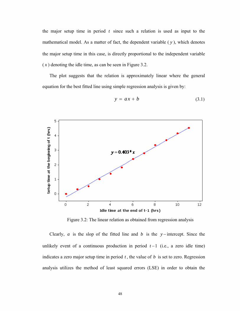
48
the major setup time in period t since such a relation is used as input to the
mathematical model. As a matter of fact, the dependent variable ( y ), which denotes
the major setup time in this case, is directly proportional to the independent variable
( x ) denoting the idle time, as can be seen in Figure 3.2.
The plot suggests that the relation is approximately linear where the general
equation for the best fitted line using simple regression analysis is given by:
y a x b= + (3.1)
Figure 3.2: The linear relation as obtained from regression analysis
Clearly, a is the slop of the fitted line and b is the y − intercept. Since the
unlikely event of a continuous production in period 1t − (i.e., a zero idle time)
indicates a zero major setup time in period t , the value of b is set to zero. Regression
analysis utilizes the method of least squared errors (LSE) in order to obtain the

49
optimized value of the slope, which yields a value for 0.403a = using the MINITAB
software after setting 0b = .
We next present the mathematical formulation for the production planning
problem at hand. This operational model establishes the raw material purchasing
quantities, regular time and overtime based production quantities, inventory levels,
backorder and substitution quantities for each product in each time period such that
the total cost over the planning horizon is minimized. In developing the mathematical
model, quantities of materials, whether billets or rebars, are measured in tons and the
production rate is measured in tons per hour. An index, whether i for raw material
(RM) or j for finished product (FP), refers to the same dimension in both steel
grades (SG). This notation greatly assists in formulating the problem as a
mathematical model.
The model seeks to minimize the total costs incurred in addition to the penalties
resulting from downward substitution. The total cost is composed of RM ordering,
RM purchasing, RM inventory holding, setup, regular time production, overtime
production, FP holding and backorder costs. The last term in the objective function is
an additional penalty term which ensures that demand substitution is further
discouraged since in this case the higher grade steel is sold at the price of the lower
quality one entailing a lost profit to the company. The objective function along with
the set of constraints involved is set out as follows:
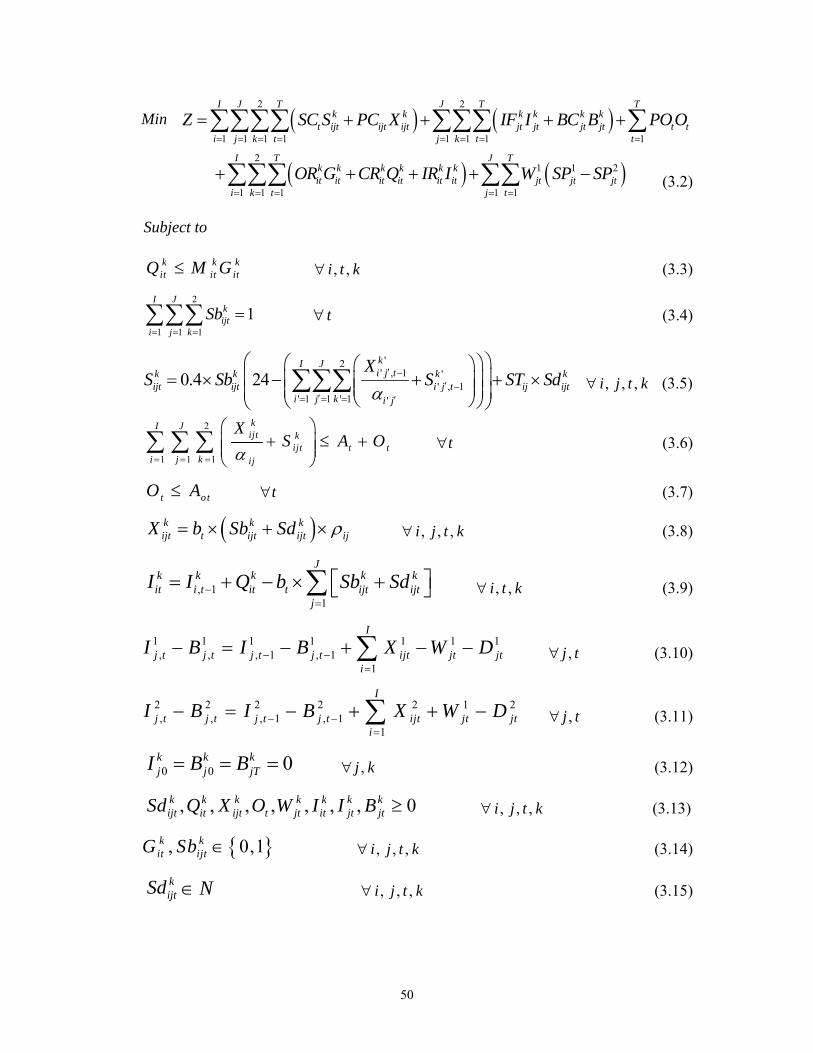
50
( ) ( )
( ) ( )
2 2
1 1 1 1 1 1 1 1
21 1 2
1 1 1 1 1
I J T J T Tk k k k k k
t ijt ijt ijt jt jt jt jt t ti j k t j k t t
I T J Tk k k k k kit it it it it it jt jt jt
i k t j t
Z SC S PC X IF I BC B POO
OR G CR Q IR I W SP SP
= = = = = = = =
= = = = =
= + + + +
+ + + + −
∑∑∑∑ ∑∑∑ ∑
∑∑∑ ∑∑
Subject to k k k
it it itQ M G≤ , ,i t k∀ (3.3)
2
1 1 1
1I J
kijt
i j k
Sb= = =
=∑∑∑ t∀ (3.4)
'2
' , 1 '' , 1
' 1 1 ' 1 '
0.4 24kI Ji j tk k k k
ijt ijt i j t ij ijti j k i j
XS Sb S ST Sd
α′ −
′ −′= = = ′
⎛ ⎞⎛ ⎞⎛ ⎞⎜ ⎟= × − + + ×⎜ ⎟⎜ ⎟⎜ ⎟⎜ ⎟⎜ ⎟⎝ ⎠⎝ ⎠⎝ ⎠
∑∑∑ , , ,i j t k∀ (3.5)
2
1 1 1
kI Jijt k
ijt t ti j k ij
XS A O
α= = =
⎛ ⎞+ ≤ +⎜ ⎟⎜ ⎟
⎝ ⎠∑ ∑ ∑ t∀ (3.6)
t otO A≤ t∀ (3.7)
( )k k kijt t ijt ijt ijX b Sb Sd ρ= × + × , , ,i j t k∀ (3.8)
, 11
Jk k k k kit i t it t ijt ijt
jI I Q b Sb Sd−
=
⎡ ⎤= + − × +⎣ ⎦∑ , ,i t k∀ (3.9)
1 1 1 1 1 1 1
, , , 1 , 11
I
j t j t j t j t ijt jt jti
I B I B X W D− −=
− = − + − −∑ ,j t∀ (3.10)
2 2 2 2 2 1 2, , , 1 , 1
1
I
j t j t j t j t ijt jt jti
I B I B X W D− −=
− = − + + −∑ ,j t∀ (3.11)
0 0 0k k kj j jTI B B= = = ,j k∀ (3.12)
, , , , , , , 0k k k k k k kijt it ijt t jt it jt jtSd Q X O W I I B ≥ , , ,i j t k∀ (3.13)
{ }, 0,1k kit ijtG Sb ∈ , , ,i j t k∀ (3.14)
kijtSd N∈ , , ,i j t k∀ (3.15)
(3.2)
Min
51
• Constraint set (3.3) ensures that the quantity of each RM i purchased in time
period t, if any, is limited by the supplier capacity in that period. This ‘fixed
charge’ constraint establishes the relation between the binary and continuous
purchasing-related variables.
• Only one major setup for a certain RM, FP and SG combination can take place
during a time period, which is stated in constraint set (3.4).
• Equation (3.5) specifies the total setup time for a certain ( , ,i j k ) combination in
any period, which is simply the sum of both major and minor setup times. The
total production and setup times are subtracted from the available 24 hours a day
to give the idle time. The result is then multiplied by 0.4, which is the coefficient
obtained earlier using regression analysis, and by the binary major setup variable
to indicate that only the chosen ( , ,i j k ) combination shall contribute to the total
setup time.
• Constraint set (3.6) states that the total production and setup times for all products
should not exceed the available uptime, whether regular production time or
overtime, in any time period.
• Naturally, the maximum number of overtime hours worked per day is bounded by
a certain allowable value, as specified by constraint (3.7).
• Since the steel bars rolling industry is a batch process, the production quantity of
a certain FP from a particular RM, kijtX , is a function of the number of batches
produced, batch size and the yield, which is stated in constraint (3.8). In fact,
Constraint set (3.8) coupled with equation (3.5) ensure the overlap of the longest
minor setup with the major setup. That is, the first batch produced at the

52
beginning of the day is for that RM-FP combination that requires the longest
minor setup time.
• Constraint set (3.9) defines the inventory balance equation for a particular RM i at
the end of time period t as the sum of the previous period’s stock balance and the
quantity procured in the current period minus the quantity consumed in the
production of the various end items in the current period.
• Constraint sets (3.10) and (3.11) provide the finished products inventory balance
equations for both steel grades. Depending on its economic feasibility, these
constraints allow for the demand of a grade 40 steel bar to be partially fulfilled by
a similar sized grade 60 rebar. The inventory balance equations for both grades
are better understood using Figure 3.3 below.
Figure 3.3: Inventory balance for both grades in a particular time period
• Without loss of generality, the initial inventory and backorder levels are set to
zero as shown in constraint (3.12) which also ensures that the demand for all the
finished products throughout the planning horizon is met through setting the
ending backorder levels to zero.
Period t Grade 60
(k=1)
1,j tI
1,j tB
1, 1j tI −
1, 1j tB −
1
1
I
ijti
X=∑
1jtD 1
jtW
Period t Grade 40
(k=2)
2,j tI
2,j tB
2, 1j tI −
2, 1j tB −
2
1
I
ijti
X=∑
2jtD
1jtW

53
• Constraints (3.13) – (3.15) represent the non-negativity, binary and integrality
restrictions on the respective decision variables.
It should also be noted that, in any time period, the consumption rate of a specific raw
material to produce the various finished products should not exceed the purchased
quantity of that raw material in that same period in addition to the previously
available stock. That is
, 11
Jk k k k
t ijt ijt it i tj
b Sb Sd Q I −=
⎡ ⎤× + ≤ +⎣ ⎦∑ , ,i t k∀ (3.16)
However, constraint set (3.16) is implied by constraint set (3.9) along with the non-
negativity restriction on the variables kitI .
3.5 Properties of the Mathematical Model
The model developed above is, in a sense, a typical dynamic capacitated multi-
item lot-sizing problem (CMILSP) formulation with various practical extensions
incorporated into the model. A much simpler version, which is the capacitated single-
item lot-sizing problem (CSILSP), is NP-hard in general. It is even NP-hard for very
special cases (Bitran and Yanasse 1982). As pointed out by Maes and Van
Wassenhove (1986), capacitated lot-sizing models are powerful and very flexible but
slow (or impossible) to solve if the problem instance is very large. Prior to
establishing the solution methodology for the mathematical model, the properties of
the model have to be explored in order to gain more insights towards solving the
model. These properties are:
54
• Non-separable: Although the two steel grades share the same combination of
dimensions for both RM and FP, the problem is not separable into two smaller
sub-problems each dealing with one steel grade at a time. This is the case since it
is not known in advance how much capacity should be allocated to each steel
grade, and this would also eliminate the possibility for demand substitution.
• Bilinear program: Clearly, the model at hand is a mixed integer nonlinear
program (MINLP) as it involves a mixture of continuous and integer variables,
and the non-linearity arises due to the existence of a nonlinear constraint
(Equation 3.5) that also appears in the objective function (once the variable kijtS is
substituted for by its expression). In particular, the model falls under a special
category of nonlinear programs called mixed integer bilinear programs (MIBLP)
in which the binary variable kijtSb is multiplied by the continuous variables '
' , 1ki j tX ′ −
and '' , 1ki j tS ′ − , one at a time, as can be seen in equation (3.5). The bilinearity
property these models possess is due to the fact that, for fixed kijtSb values, the
original model reduces to a mixed integer linear program (MILP), and for fixed
'' , 1ki j tX ′ − and '
' , 1ki j tS ′ − values, it again reduces to a MILP in the space of the other
decision variables. Such models have also been addressed in the literature under
the title “mixed 0-1 quadratic programs” (e.g., Adams et al. 2004, Adams and
Forrester 2007).
• Non-convexity: In the context of nonlinear programming, the simplest
mathematical models to obtain a solution for are the convex programs, which
involve the minimization of a convex function subject to a convex set. In such a

55
case, classical optimization techniques can be used to obtain the optimal solution,
where the local optimum coincides with the global one. Unfortunately, the
bilinearity existent in the model above causes it to be non-convex as we shall
prove in what follows. In order to prove non-convexity of the model, it suffices to
show that either the objective function is non-convex or that the feasible region,
as defined by the set of constraints, is not a convex set. Since a linear function is
both convex and concave, we target constraint (3.5) and show that it is not convex
which entails that the feasible region is not a convex set. For a function to be non-
convex, its Hessian matrix must not be positive definite or positive semidefinite.
First, let us rearrange the terms in constraint (3.5) and rewrite it as follows:
2
, 1, 1
1 1 1
9.6 0.4 0kI Jij tk k k k k
ijt ijt ijt ij t ij ijti j k ij
XS Sb Sb S ST Sd
α−
−= = =
⎛ ⎞− × + × + + × =⎜ ⎟⎜ ⎟
⎝ ⎠∑∑∑ (3.17)
Let the left hand side (LHS) above be denoted as , 1 , 1( , , , , )k k k k kijt ijt ij t ij t ijtg S Sb X S Sd− −
and assume, for the time being, that this function is twice differentiable (i.e., relax
the integrality and binary restriction on the respective decision variables). Then,
the vector of the first order partial derivatives (i.e., the gradient) is given by:
2, 1
, 11 1 1
, 1
, 1
1
9.6 0.4
0.4
0.4
kk I Jij t kijt
ij tki j k ijijt
kij t k
ijtkijij t
k kijt ijt
ij
XS SSb
XgSb
SSd Sb
ST
α
α
−−
= = =
−
−
⎛ ⎞⎜ ⎟
⎛ ⎞⎛ ⎞ ⎜ ⎟− + +⎜ ⎟⎜ ⎟ ⎜ ⎟⎜ ⎟⎝ ⎠⎜ ⎟ ⎜ ⎟
⎜ ⎟ ⎜ ⎟∇ =⎜ ⎟ ×⎜ ⎟⎜ ⎟ ⎜ ⎟⎜ ⎟ ⎜ ⎟×⎝ ⎠ ⎜ ⎟
⎜ ⎟⎝ ⎠
∑ ∑∑
(3.18)
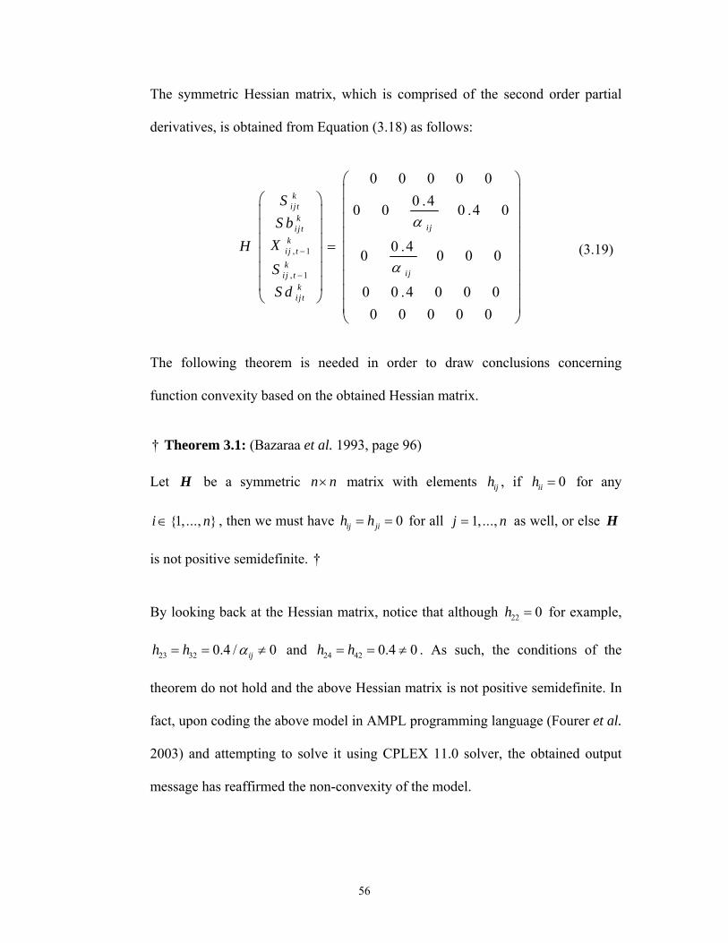
56
The symmetric Hessian matrix, which is comprised of the second order partial
derivatives, is obtained from Equation (3.18) as follows:
, 1
, 1
0 0 0 0 00 .40 0 0 .4 0
0 .40 0 0 0
0 0 .4 0 0 00 0 0 0 0
ki j t
ki ji j t
ki j tk
i ji j tki j t
SS b
XHSS d
α
α−
−
⎛ ⎞⎜ ⎟⎛ ⎞ ⎜ ⎟⎜ ⎟ ⎜ ⎟⎜ ⎟ ⎜ ⎟⎜ ⎟ = ⎜ ⎟⎜ ⎟ ⎜ ⎟⎜ ⎟ ⎜ ⎟⎜ ⎟ ⎜ ⎟⎝ ⎠⎜ ⎟⎝ ⎠
(3.19)
The following theorem is needed in order to draw conclusions concerning
function convexity based on the obtained Hessian matrix.
† Theorem 3.1: (Bazaraa et al. 1993, page 96)
Let H be a symmetric n n× matrix with elements ijh , if 0iih = for any
{1,..., }i n∈ , then we must have 0ij jih h= = for all 1, ...,j n= as well, or else H
is not positive semidefinite. †
By looking back at the Hessian matrix, notice that although 22 0h = for example,
23 32 0.4 / 0ijh h α= = ≠ and 24 42 0.4 0h h= = ≠ . As such, the conditions of the
theorem do not hold and the above Hessian matrix is not positive semidefinite. In
fact, upon coding the above model in AMPL programming language (Fourer et al.
2003) and attempting to solve it using CPLEX 11.0 solver, the obtained output
message has reaffirmed the non-convexity of the model.

57
In brief, the presented mathematical model is a non-separable, non-convex, mixed
integer bilinear program. These complicating features of the mathematical model
explain the incapability of the commercial off-the-shelf optimization packages (e.g.,
AMPL/CPLEX and LINGO) to directly obtain the solution to this class of models
even for small problem instances. Hence, there is a need for a specifically tailored
solution algorithm that can efficiently handle such class of mathematical models as
shall be presented in the next chapter.
3.6 Summary
This chapter has discussed the production planning problem encountered on a
frequent basis at the maser production scheduling level in steel rolling mills. The
problem was formulated as a MIBLP in which the technological constraints
associated with the manufacturing process have been taken into account. The model
studies the combined effects of several interrelated factors characterizing this type of
industry such as complex setup time structure, batch production, scrap rate, overtime,
backlogging and product substitution, on the planning decisions. The objective is to
establish the daily/weekly production lot sizes such that the assumed static customer
demand is fulfilled at a minimal total cost. Upon studying the properties of the
presented mathematical model, it turned out that such model is not readily solvable
using the commercial optimization packages. Our efforts in the next chapter are
directed towards developing efficient solution algorithms that have the ability to solve
similar models within a reasonable amount of computational time.

58
Chapter 4
Application of the Solution Methodologies to the Proposed
Mathematical Model
4.1 Introduction
This chapter seeks to attain the solution to the production planning model through
the implementation and/or customization of the solution techniques discussed in the
appendix. In general, solving the equivalent MILP resulting from the linearization
approaches directly using the MIP solver or obtaining the solution to the bilinear
model via branch-and-bound (B&B) algorithms yield an optimal solution unless the
solver is stopped after a pre-specified length of run time where the solution is
considered satisfactory in this case. Benders decomposition (BD) approach, on the
other hand, does not necessarily render an optimal solution depending on the value set
for the accepted tolerance. We start by presenting how a generic linearization
approach applies to the model at hand followed by the development of a modified
B&B algorithm and lastly a hybrid linearization-BD approach. In this chapter, the
solutions obtained to the model at hand via these solution techniques are the optimal
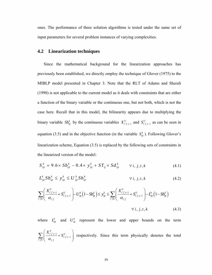
59
ones. The performance of three solution algorithms is tested under the same set of
input parameters for several problem instances of varying complexities.
4.2 Linearization techniques
Since the mathematical background for the linearization approaches has
previously been established, we directly employ the technique of Glover (1975) to the
MIBLP model presented in Chapter 3. Note that the RLT of Adams and Sherali
(1990) is not applicable to the current model as it deals with constraints that are either
a function of the binary variable or the continuous one, but not both, which is not the
case here. Recall that in this model, the bilinearity appears due to multiplying the
binary variable kijtSb by the continuous variables '
' , 1ki j tX ′ − and '
' , 1ki j tS ′ − as can be seen in
equation (3.5) and in the objective function (in the variable kijtS ). Following Glover’s
linearization scheme, Equation (3.5) is replaced by the following sets of constraints in
the linearized version of the model:
9.6 0.4k k k kijt ijt ijt ij ijtS Sb y ST Sd= × − × + × , , ,i j t k∀ (4.1)
k k k k kijt ijt ijt ijt ijtL Sb y U Sb≤ ≤ , , ,i j t k∀ (4.2)
( ) ( )' '
' , 1 ' , 1' '' , 1 ' , 1
' ' ' '' '
1 1k ki j t i j tk k k k k k k
i j t ijt ijt ijt i j t ijt ijti j k i j ki j i j
X XS U Sb y S L Sb
α α′ ′− −
′ ′− −′ ′′ ′
⎛ ⎞ ⎛ ⎞+ − − ≤ ≤ + − −⎜ ⎟ ⎜ ⎟⎜ ⎟ ⎜ ⎟
⎝ ⎠ ⎝ ⎠∑ ∑
, , ,i j t k∀ (4.3)
where kijtL and k
ijtU represent the lower and upper bounds on the term
'' , 1 '
' , 1' ' '
ki j t k
i j ti j k i j
XS
α′ −
′ −′ ′
⎛ ⎞+⎜ ⎟⎜ ⎟
⎝ ⎠∑ respectively. Since this term physically denotes the total
60
production and setup time in period 1t − , the value of the lower bound, kijtL , is simply
set to zero and that for the upper bound is kijt t otU A A= + , which is the total available
regular and overtime hours of production capacity.
Constraints (4.1) – (4.3) are necessary in order to establish the equivalence
'' , 1 '
' , 1' ' '
ki j tk k k
ijt ijt i j ti j k i j
Xy Sb S
α′ −
′ −′ ′
⎛ ⎞= +⎜ ⎟⎜ ⎟
⎝ ⎠∑ for all , ,i j t and k . Once the binary variables
kijtSb assume a value of zero, constraint set (4.2) is binding while constraint set (4.3) is
the binding one whenever kijtSb assume a value of one. Since the newly added
variables, kijty , appear in the objective function with a negative sign, the model will
seek the maximum possible value for this variable. This indicates that the left hand
side inequalities of constraints (4.2) and (4.3) are redundant and can be dropped out
of the model.
Clearly, the linearization approaches, in general, suffer from a common drawback
that affects their performance. They involve a radical increase in the number of
problem variables and constraints and, as such, the gains to be derived from dealing
with linear functions are quite likely to be nullified by the increased problem size
(Glover 1975). This increase in the problem size has a major impact on the CPU
computation time especially for large scale models since the added variables and
constraints are accounted for at all branching nodes in the MIP solver. In particular,
the linearized version of the model at hand involves the addition of I J T K× × ×
variables and 2 I J T K× × × × constraints. The performance of the linearization
approach for several problem instances of different sizes is reported in Section 4.5.

61
4.3 Modified Branch-and-Bound algorithm
The production planning problem at hand, like many other real world problems, is
a combinatorial optimization problem that has a very large, but finite, number of
feasible solutions. However, solving such discrete optimization problems to
optimality through explicit enumeration is normally impossible or is an immense job
requiring substantial amount of computational time. For the linearization approach
discussed earlier, the shortcomings associated with this approach contribute to a much
needed alternative and a more efficient solution procedure.
In this section, a modified version of the long established B&B algorithm is
developed in which different branching, bounding and fathoming strategies are
employed. The basic idea here is to get rid of bilinearity through proper substitution
of the complicating binary variables, kijtSb , while simultaneously obtaining the bound
at each node via such substitution. Once the values of these variables are set to either
zero or one, the resulting reduced size MILP becomes a lot easier to solve.
Fortunately, constraint set (3.4) states that among all possible RM, FP and SG
combinations, there exists only one possible combination for which a major setup
could take place in period t . Hence, setting '' ' 1k
i j tSb = for a certain value of 'i , 'j and
'k entails that 0kijtSb = for either one of 'i i≠ , 'j j≠ , 'k k≠ and for the same t .
This reduces the number of possibilities (i.e. branches to be explored) to I J K× × for
each t . Moreover, the possible number of 1kijtSb = combinations at optimality is now
( )TIJK as a direct result of constraint (3.4). However, fully exploring this many
possibilities is a tedious and a time consuming task especially for large scale models.

62
Therefore, a clever enumeration algorithm for such possibilities is much needed. The
proposed B&B based solution algorithm is stated formally as follows:
Step 1: Set 0kijtSb = for , , ,i j k t∀ throughout the model, ignore Equation (3.4) and
then solve.
The resulting MILP problem is a relaxed version of the original problem and its
solution provides a lower bound on the optimal value for the original problem since
the major setup cost is set to zero. However, its solution is not feasible to the original
problem as it violates equation (3.4).
Step 2: Set 1t = and substitute 1 1kijSb = for each branch emanating from the original
node, with I J K× × possible branches, while keeping the substitution 0kijtSb = for
, ,i j k∀ and 1t > .
The resulting solution to each of these subproblems gives a lower bound on the
optimal objective function value of the original problem. Among the resulting
I J K× × subproblems, branch from the one with the lowest value of the objective
function, as this is the most promising node (ties are broken arbitrarily).
Step 3: Repeat step 2 for 2,3,...,t T= with each value of t corresponding to one level
in the tree. Again, there would be I J K× × possible branches from each node.
Clearly, the lower bound on the optimal objective function value increases as we go
down the tree since larger portions of the major setup cost are being accounted for.
Step 4: The solution with the minimum objective function value obtained at the
lowest level of the tree (corresponding to t T= ) is called the incumbent, which is
used as an upper bound during the search of the unexplored branches of the tree. The
search continues with other branches and the value of this incumbent is compared
63
with the bounds obtained at each node in order to make the fathoming decisions. If
the value of the objective function calculated at a particular node is larger than the
incumbent, that branch is fathomed. Otherwise, the value of the incumbent is updated
whenever a lower value incumbent is attained, and then the new incumbent is used to
make the fathoming decisions.
It should be noted that at each node of the tree, the MILP model is solved without
equation (3.4) but it is this constraint that drove the branching scheme in the first
place. The tree exploring strategy is depth-first since this allows a faster recovery of
an incumbent, which can be used to make the fathoming decisions. The width of the
tree depends on the values of I , J and K , and the number of different levels is equal
to 1T + . The obtained MILP models at each node are directly solved using
AMPL/CPLEX 11.0 solver.
To serve illustrative purposes, Figure 4.1 depicts a graphical representation for the
progress of the proposed algorithm as applied to a small problem instance ( 2I K= = ,
3J = and 4T = ). Implementing the algorithm yields a tree with 5 levels (since
1 5T + = ) and 12 nodes (since 12I J K× × = ) at each level starting from level 2. The
nodes shown with a solid line are the ones yielding the minimum objective function
value (i.e. most promising) among all other nodes in the same level. The branches in
the solid line represent the path connecting these nodes which leads to the incumbent
at the bottom of the tree. Hence, the values of the major setup variables corresponding
to the incumbent in Figure 4.1 are 2 1 2 2221 232 113 224 1Sb Sb Sb Sb= = = = . The incumbent
value can now be used to make the fathoming decisions for the unexplored branches

64
of the tree, which could eventually result in an optimal solution different from the
current incumbent (indicating that a lower value incumbent has been found).
Figure 4.1: Partial tree resulting from applying the proposed B&B algorithm for a small problem instance
At this juncture, a clear distinction has to be made between the classical B&B
algorithm and the one proposed in this work. The classical B&B algorithm utilizes
LP-relaxation of the binary variables kijtSb in order to obtain the bound at the initial
node. Such a relaxation does not resolve either bilinearity or non-convexity embedded
in the model and hence the resulting model is still not directly solvable using
optimization software. As a matter of fact, the relaxed version of the model is now
“pure bilinear” (two continuous variables are multiplied by one another) instead of
2111 1Sb = 1
121 1Sb = 2221 1Sb = 1
231 1Sb = 1111 1Sb = 2
231 1Sb =
2112 1Sb = 1
122 1Sb = 2222 1Sb = 1
232 1Sb = 1112 1Sb = 2
232 1Sb =
2113 1Sb = 1
123 1Sb = 2223 1Sb = 1
233 1Sb = 1113 1Sb = 2
233 1Sb =
2114 1Sb = 1
124 1Sb = 2224 1Sb = 1
234 1Sb = 1114 1Sb = 2
234 1Sb =
0kijtSb =, , ,i j t k∀
. . . . . . . . . . . .
. . . . . . . . . . . .
. . . . . . . . . . . . .
. . . . . . . . . . . . .

65
being “mixed-integer bilinear”, and there exists a reformulation-linearization
technique established in the literature for this class of bilinear models (Sherali and
Alameddine 1992). Table 4.1 provides more insights into the differences between the
classical B&B algorithm and the modified one.
Table 4.1: A comparison between the classical B&B algorithm and the modified B&B algorithm proposed in this thesis
Classical B&B Modified B&B
Branching
- Two branches emanate from each node corresponding to one of the binary variables being assigned a value of either zero or one (Except at an incumbent or at an integer solution where no more branching takes place).
- Hence, the number of nodes at
any level of the tree is twice that of the higher level.
- Utilizes Constraint (3.4) to obtain I J K× × branches from each node, where each branch corresponds to one of the binary variables being equal to one.
- Each level in the tree corresponds to a single t value.
- This branching scheme results
in a tree with I J K× × nodes at each level of the tree.
Bounding
Relaxes the binarity restriction on all binary variables (except the branching variable) and allows those variables to assume any value between zero and one (i.e. LP relaxation).
Assumes the values of all binary variables (other than the branching variable) are set to zero (those in the same level are set to zero due to constraint (3.4) and others to obtain the bound and reduce the original problem to a MILP).
Incumbent Corresponds to an integer solution obtained at any node (this might
occur at any level of the tree)
Obtained only at the lowest level of the tree, since that is
when Constraint (3.4) is satisfied
It is important to point out that there exist several practical problems to which the
proposed B&B based algorithm is applicable. Examples include, but not limited to:
(1) Small-bucket dynamic lot-sizing problems where a single product may be

66
produced in each time period, (2) Portfolio management problems where a new
investment opportunity is decided upon at the beginning of each year, and (3) Vendor
selection problem where a product may be solely supplied by a single source for a
specific time period. Section 4.5 presents a numerical example for a small problem
instance as well as the computational experiments for various problem sizes.
4.4 Hybrid Linearization-Benders decomposition approach
The solution algorithm presented in this section is a two phase methodology that
first applies the linearization approach in order to obtain the linearized model and
then applies Benders decomposition (BD) to this MILP model instead of solving it
directly via the MIP solver. The motivation to use BD is its ability to handle the
complicating variables separately which is likely to save in the computational time
needed. More importantly, we seek to provide an application of BD to the solution of
mathematical models involving complicating constraints as well (constraint 3.5 in this
case). On page 244 of their book, Conejo et al. (2006) point out that considering
nonlinear constraints as complicating constraints and treating them through
linearization procedures do not lead generally to a decomposed problem. Therefore,
we present an instance of a mathematical model to which linearization techniques are
applied first and then the linearized model is handled with Benders decomposition
approach.
Following the BD methodology, the complicating variables in the model at hand
are the binary variables kijtSb and k
itG , as well as the integer variables kijtSd . Since the
continuous variables kijtS and k
ijtX are functions of the kijtSb and k
ijtSd variables as can

67
be seen in equations (3.5) and (3.8) respectively, their values are optimized via
solving the master problem which is given by:
Master problem:
( )
( )
2
1 1 1 1
2
1 1 1
I J Tk k
MP t ijt ijt ijti j k t
I Tk k k k k kit it it it it it
i k t
Z SC S PC X
OR G CR Q IR I α
= = = =
= = =
= +
+ + + +
∑∑∑∑
∑∑∑
Subject to
( ) ( )( ) ( ) ( ) ( )( ) v v v vv k k k k k k
SP ijt ijt ijt ijt ijt ijtijtk ijtk
Z S S X Xα μ λ≥ + − + −∑ ∑ 1, ...,v V= (4.5)
k k kit it itQ M G≤ , ,i t k∀ (4.6)
2
1 1 1
1I J
kijt
i j k
Sb= = =
=∑∑∑ t∀ (4.7)
9.6 0.4k k k kijt ijt ijt ij ijtS Sb y ST Sd= × − × + × , , ,i j t k∀ (4.8)
k k k k kijt ijt ijt ijt ijtL Sb y U Sb≤ ≤ , , ,i j t k∀ (4.9)
( ) ( )' '
' , 1 ' , 1' '' , 1 ' , 1
' ' ' '' '
1 1k ki j t i j tk k k k k k k
i j t ijt ijt ijt i j t ijt ijti j k i j ki j i j
X XS U Sb y S L Sb
α α′ ′− −
′ ′− −′ ′′ ′
⎛ ⎞ ⎛ ⎞+ − − ≤ ≤ + − −⎜ ⎟ ⎜ ⎟⎜ ⎟ ⎜ ⎟
⎝ ⎠ ⎝ ⎠∑ ∑
, , ,i j t k∀ (4.10)
( )k k kijt t ijt ijt ijX b Sb Sd ρ= × + × , , ,i j t k∀ (4.11)
, 11
Jk k k k kit i t it t ijt ijt
jI I Q b Sb Sd−
=
⎡ ⎤= + − × +⎣ ⎦∑ , ,i t k∀ (4.12)
, , , , 0k k k kijt it ijt itSd Q X I α ≥ , , ,i j t k∀ (4.13)
{ }, 0,1k kit ijtG Sb ∈ , , ,i j t k∀ (4.14)
kijtSd N∈ , , ,i j t k∀ (4.15)
(4.4)Min

68
Notice that the variable α assumes only non-negative values (Constraint 4.13)
since it represents an underestimate for the sub-problem’s cost function. Once the
values of the complicating variable are established, they are substituted into the sub-
problem in order to optimize the production capacity, finished product inventory and
backlogging, and the substitution related decisions. The sub-problem at iteration v is
formulated below:
Sub-problem:
( )
( )
2( )
1 1 1 1
1 1 2
1 1
T J Tv k k k k k k
SP t t jt jt jt jt jt jtt j k t
J T
jt jt jtj t
Z PO O IF I BC B M R
W SP SP
= = = =
= =
= + + +
+ −
∑ ∑∑∑
∑∑
Subject to
2
1 1 1
kI Jijt k
ijt t ti j k ij
XS A O
α= = =
⎛ ⎞+ ≤ +⎜ ⎟⎜ ⎟
⎝ ⎠∑ ∑ ∑ t∀ (4.17)
t otO A≤ t∀ (4.18)
1 1 1 1 1 1 1 1, 1 , 1 , ,
1
I
j t j t j t j t ijt jt jt jti
I B I B X W R D− −=
− − + + − + =∑ ,j t∀ (4.19)
2 2 2 2 2 2, , , 1 , 1
1
I
j t j t j t j t ijt jti
I B I B X W− −=
− = − + −∑ ,j t∀ (4.20)
1 2 2 2jt jt jt jtW W R D+ + = ,j t∀ (4.21)
0 0 0k k kj j jTI B B= = = ,j k∀ (4.22)
, , , , 0k k k kt jt jt jt jtO W I B R ≥ , ,j t k∀ (4.23)
( )vk k
ijt ijtS S= : ( )vk
ijtμ , , ,i j t k∀ (4.24)
( )vk k
ijt ijtX X= : ( )vk
ijtλ , , ,i j t k∀ (4.25)
(4.16)
Min
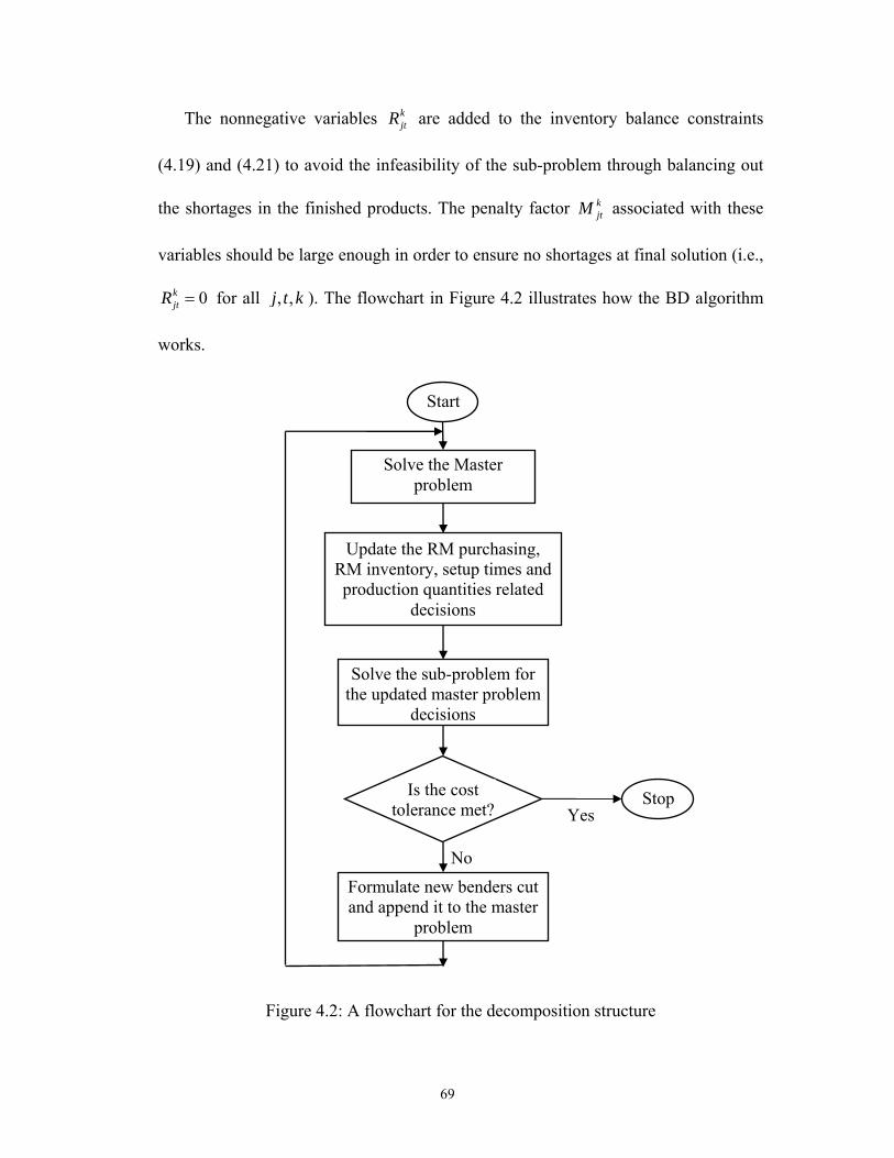
69
The nonnegative variables kjtR are added to the inventory balance constraints
(4.19) and (4.21) to avoid the infeasibility of the sub-problem through balancing out
the shortages in the finished products. The penalty factor kjtM associated with these
variables should be large enough in order to ensure no shortages at final solution (i.e.,
0kjtR = for all , ,j t k ). The flowchart in Figure 4.2 illustrates how the BD algorithm
works.
Figure 4.2: A flowchart for the decomposition structure
Start
Solve the Master problem
Update the RM purchasing, RM inventory, setup times and production quantities related
decisions
Solve the sub-problem for the updated master problem
decisions
Formulate new benders cut and append it to the master
problem
Is the cost tolerance met? Stop
No
Yes
70
The solution to the sub-problem provides marginal information on the goodness
of the decisions made at the master problem which is reflected in the obtained values
for the associated dual variables. After each iteration v , those dual variables are fed
back into the master problem, through the optimality cut (constraint 4.5), which helps
refine the decisions made at the previous iteration. Note that only the variables kijtS
and kijtX need to be included in the optimality cut since they are the only variables
from the master problem that appear in the sub-problem and can affect the sub-
problem’s objective function value. The addition of any other variable (e.g., kijtSb and
kijtSd ) to the optimality cut will result in a zero value for their associated dual
variables in all the iterations, and consequently, this would not have any impact on
the solution or the convergence rate. As mentioned in the appendix, the algorithm
terminates when the cost tolerance ( ) ( )v vSPZ α ε− < is met.
4.5 Computational analysis
The purpose of this section is to provide more insights into the mechanism of the
proposed B&B algorithm through a simple numerical example. Also, the performance
of the three solution algorithms is benchmarked against one another for several
problem instances of varying complexities.
4.5.1 A numerical example
To serve for illustrative purposes, a relatively small problem instance where
2I K= = , 3J = and 4T = is solved in this subsection through applying the B&B
algorithm. Table 4.2 shows problem parameters involving only the time index, which

71
are available regular time and overtime capacity, batch size, the per hour overtime
cost and setup cost. Since higher values for the index j indicate smaller rebar
diameters (see Table 3.2), the per unit production cost from the same billet (i.e. same
i) increases for increasing values of j as seen in Table 4.3. The finished product
related parameters, including inventory holding cost, backordering cost, selling prices
and demand are shown in Tables 4.4 and 4.5. On the other hand, Table 4.6 provides
the values for the raw material related parameters, including procurement cost,
ordering cost, inventory holding cost and maximum supply capacity. Finally, Table
4.7 gives the yields, production rates and minor setup times for each raw material-
finished product combination.
Table 4.2: Problem parameters involving only time index
Time period tA otA tb tPO tSC
t = 1 16 4 60 300 400 t = 2 16 4 60 300 400 t = 3 16 4 60 300 400 t = 4 16 4 60 300 400
Table 4.3: Production cost
i = 1 i = 2 ijtPC
j = 1 j = 2 j = 3 j = 1 j = 2 j = 3 t = 1 25 30 35 20 26 30 t = 2 25 30 35 20 26 30 t = 3 25 30 35 20 26 30 t = 4 25 30 35 20 26 30
Table 4.4: Inventory holding and backordering costs
kjtIF k
jtBC
j = 1 j = 2 j = 3 j = 1 j = 2 j = 3
Time
Period k = 1 k = 2 k = 1 k = 2 k = 1 k = 2 k = 1 k = 2 k = 1 k = 2 k = 1 k = 2
t = 1 32 30 35 33 39 37 25 25 28 28 34 34 t = 2 33 31 36 34 41 39 26 26 30 30 35 35 t = 3 30 28 33 31 40 38 27 27 32 32 37 37 t = 4 32 30 35 33 41 39 30 30 34 34 38 38

72
Table 4.5: Demand and selling prices for end items
kjtSP
kjtD
j = 1 j = 2 j = 3 j = 1 j = 2 j = 3
Time
Period k = 1 k = 2 k = 1 k = 2 k = 1 k = 2 k = 1 k = 2 k = 1 k = 2 k = 1 k = 2
t = 1 1800 1600 1830 1630 1900 1700 60 130 100 90 60 100 t = 2 1800 1600 1830 1630 1900 1700 70 100 120 55 110 75 t = 3 1840 1640 1860 1660 1940 1740 90 85 80 110 95 40 t = 4 1820 1620 1860 1660 1930 1730 140 70 90 150 65 50
Table 4.6: Raw material related costs and supplying limits
kitCR k
itOR kitIR k
itM i = 1 i = 2 i = 1 i = 2 i = 1 i =2 i = 1 i = 2
Time
Period k = 1 k = 2 k = 1 k = 2 k = 1 k = 2 k = 1 k = 2 k = 1 k = 2 k = 1 k = 2 k = 1 k = 2 K = 1 k = 2
t = 1 650 550 700 600 2000 2000 2200 2200 22 20 25 23 300 300 300 300t = 2 660 560 710 610 2050 2050 2250 2250 23 21 26 24 300 300 300 300t = 3 640 540 700 600 2100 2100 2300 2300 22 20 25 23 300 300 300 300t = 4 670 570 720 620 2100 2100 2300 2300 23 21 26 24 300 300 300 300
Table 4.7: Yields, production rates and minor setup times
ijρ ijα
ijST
Raw material
j = 1 j = 2 j = 3 j = 1 j = 2 j = 3 j = 1 j = 2 j = 3 i = 1 0.94 0.90 0.87 56 54 52 0.25 0.40 0.50 i = 2 0.96 0.93 0.91 58 56 54 0.40 0.50 0.75
Implementing the proposed solution algorithm yields a tree with 5 levels (since
1 5T + = ) and 12 nodes (since 12I J K× × = ) at each level starting from level 2 (a
partial tree is seen in Figure 4.3). At this stage of tree exploration, several branches
can already be fathomed as they yield an objective function value that is higher than
the current incumbent. In particular, starting from level 2 in the tree, the branches
emanating from the three nodes where 1 1 2211 221 221 1Sb Sb Sb= = = can be fathomed.
Several other nodes at the lower levels of the tree shall be fathomed as well. The
remaining branches (i.e., those emanating from nodes with lower objective function
value than that of the incumbent) need to be explored, and the current incumbent is to

73
2111 1Sb =
1,601,940
1121 1Sb =
1,601,570
2121 1Sb =
1,601,710
1131 1Sb =
1,601,660
2131 1Sb =
1,602,030
2211 1Sb =
1,601,710
1221 1Sb =
1,605,670
2221 1Sb =
1,603,920
1211 1Sb =
1,603,540
1231 1Sb =
1,603,350
1111 1Sb =
1,601,780
2231 1Sb =
1,601,530
2112 1Sb =
1,602,070
1122 1Sb =
1,601,830
2122 1Sb =
1,602,640
1132 1Sb =
1,601,870
2132 1Sb =
1,603,740
2212 1Sb =
1,601,980
1222 1Sb =
1,604,730
2222 1Sb =
1,605,540
1212 1Sb =
1,601,830
1232 1Sb =
1,601,960
1112 1Sb =
1,601,860
2232 1Sb =
1,601,970
2113 1Sb =
1,603,610
1123 1Sb =
1,603,690
2123 1Sb =
1,603,340
1133 1Sb =
1,603,290
2133 1Sb =
1,605,410
2213 1Sb =
1,603,340
1223 1Sb =
1,606,040
2223 1Sb =
1,605,960
1213 1Sb =
1,603,340
1233 1Sb =
1,603,100
1113 1Sb =
1,603,610
2233 1Sb =
1,603,100
2114 1Sb =
1,605,230
1124 1Sb =
1,603,600
2124 1Sb =
1,603,600
1134 1Sb =
1,603,580
2134 1Sb =
1,605,390
2214 1Sb =
1,603,600
1224 1Sb =
1,606,550
2224 1Sb =
1,606,360
1214 1Sb =
1,603,600
1234 1Sb =
1,603,560
1114 1Sb =
1,603,630
2234 1Sb =
1,603,510
1111 1Sb =
1,598,910
Figure 4.3: Partial tree resulting from applying the proposed B&B

74
be updated accordingly whenever a lower value is obtained (step 4 of the algorithm).
As it turns out, the current incumbent value dominates all other branches, with the
exception of only one branch resulting in the same objective function value (i.e.,
alternative optima). Since the planning horizon is 4 days, we would have four major
setups corresponding to one at the beginning of each day. The optimal values of these
major setup variables are 2 1 1 2231 232 233 234 1Sb Sb Sb Sb= = = = , which correspond to the first
incumbent obtained (or alternatively, 2 1 2 2231 232 233 234 1Sb Sb Sb Sb= = = = ).
Table 4.8: Finished product inventory, backorder and substitution quantities
j = 1 j = 2 j = 3
kjtI k = 1 k = 2 k = 1 k = 2 k = 1 k = 2
t = 1 0 0 0 26 0 9.2 t = 2 1 0 23 0 0 0 t = 3 26.2 12.4 0 0 13.6 0 t = 4 0.2 0 15 0 0.8 0
j = 1 j = 2 j = 3
kjtB
k = 1 k = 2 k = 1 k = 2 k = 1 k = 2 t = 1 3.6 14.8 0 0 7.8 0 t = 2 0 17.8 0 10 0.6 19.2 t = 3 0 0 3 12 0 4.6 t = 4 0 0 0 0 0 0
j = 1 j = 2 j = 3
kjtW k = 1 k = 2 k = 1 k = 2 k = 1 k = 2
t = 1 0 130 8 82 0 100 t = 2 39.4 60.6 19 36 46.6 28.4 t = 3 0 85 0 110 0 40 t = 4 0 70 0 150 0 50
Table 4.9: Optimal raw material purchasing and inventory policy
kitQ k
itG kitI
i = 1 i = 2 i = 1 i = 2 i = 1 i = 2
Time period
k = 1 k = 2 k = 1 k = 2 k = 1 k = 2 k = 1 k = 2 k = 1 k = 2 k = 1 k = 2 t = 1 240 120 0 300 1 1 0 1 0 0 0 60 t = 2 240 0 240 0 1 0 1 0 0 0 0 0 t = 3 300 300 300 300 1 1 1 1 240 180 60 120 t = 4 0 0 0 0 0 0 0 0 0 0 0 0

75
The resulting values for the rest of the decision variables are shown in Tables 4.8-
4.10 and the optimal objective function value is * 1,603,510.Z = The resulting values
of the demand substitution variables for grade 60 steel ( 1jtW ) shown in Table 4.8
indicate that, under the given parameters’ values, it is economically advantageous for
the company to consider the demand substitution option, since 112 39.4W = , 1
21 8W = ,
122 19W = and 1
32 46.6W = .
Table 4.10: Optimal setup and production related decisions
i = 1 i = 2 kijtSd
j = 1 j = 2 j = 3 j = 1 j = 2 j = 3 k = 1 k = 2 k = 1 k = 2 k = 1k = 2 k = 1 k = 2 k = 1k = 2 k = 1 k = 2
t = 1 1 0 2 2 1 0 0 2 0 0 0 1 t = 2 1 0 3 0 0 0 1 1 0 0 2 0 t = 3 0 0 1 2 0 0 2 2 0 0 1 1 t = 4 1 0 2 3 1 0 1 1 0 0 0 0
i = 1 i = 2 kijtS
j = 1 j = 2 j = 3 j = 1 j = 2 j = 3 k = 1 k = 2 k = 1 k = 2 k = 1k = 2 k = 1 k = 2 k = 1k = 2 k = 1 k = 2
t = 1 0.25 0 0.8 0.8 0.5 0 0 0.8 0 0 0 4.75t = 2 0.25 0 1.2 0 0 0 0.4 0.4 0 0 3.932 0 t = 3 0 0 0.4 0.8 0 0 0.8 0.8 0 0 4.266 0.75t = 4 0.25 0 0.8 1.2 0.5 0 0.4 0.4 0 0 0 2.471
i = 1 i = 2 kijtX
j = 1 j = 2 j = 3 j = 1 j = 2 j = 3 k = 1 k = 2 k = 1 k = 2 k = 1k = 2 k = 1 k = 2 k = 1k = 2 k = 1 k = 2
t = 1 56.4 0 108 108 52.2 0 0 115.2 0 0 0 109.2t = 2 56.4 0 162 0 0 0 57.6 57.6 0 0 163.8 0 t = 3 0 0 54 108 0 0 115.2115.2 0 0 109.2 54.6t = 4 56.4 0 108 162 52.2 0 57.6 57.6 0 0 0 54.6
4.5.2 Further computational experiments
At this juncture, a comparison between the performance of the classical
linearization approach (Glover 1975), the proposed B&B algorithm and the hybrid
linearization-BD (L-BD) algorithm is due. For a realistic problem size ( 5I T= = ,
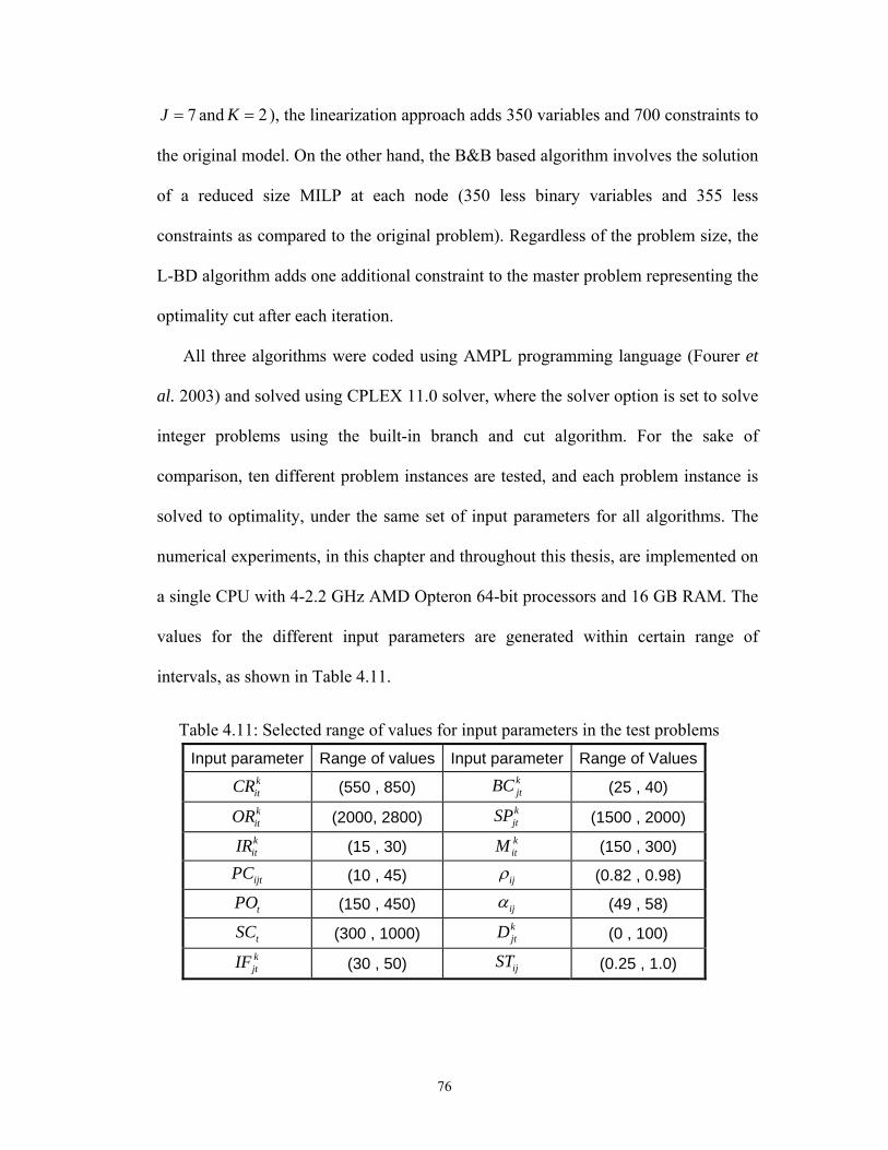
76
7J = and 2K = ), the linearization approach adds 350 variables and 700 constraints to
the original model. On the other hand, the B&B based algorithm involves the solution
of a reduced size MILP at each node (350 less binary variables and 355 less
constraints as compared to the original problem). Regardless of the problem size, the
L-BD algorithm adds one additional constraint to the master problem representing the
optimality cut after each iteration.
All three algorithms were coded using AMPL programming language (Fourer et
al. 2003) and solved using CPLEX 11.0 solver, where the solver option is set to solve
integer problems using the built-in branch and cut algorithm. For the sake of
comparison, ten different problem instances are tested, and each problem instance is
solved to optimality, under the same set of input parameters for all algorithms. The
numerical experiments, in this chapter and throughout this thesis, are implemented on
a single CPU with 4-2.2 GHz AMD Opteron 64-bit processors and 16 GB RAM. The
values for the different input parameters are generated within certain range of
intervals, as shown in Table 4.11.
Table 4.11: Selected range of values for input parameters in the test problems
Input parameter Range of values Input parameter Range of Values kitCR (550 , 850) k
jtBC (25 , 40) kitOR (2000, 2800) k
jtSP (1500 , 2000) kitIR (15 , 30) k
itM (150 , 300)
ijtPC (10 , 45) ijρ (0.82 , 0.98)
tPO (150 , 450) ijα (49 , 58)
tSC (300 , 1000) kjtD (0 , 100)
kjtIF (30 , 50) ijST (0.25 , 1.0)

77
The obtained results for the ten problem instances are reported in Table 4.12. It
should be noted that the generation of the input parameters within different ranges of
intervals will have an influence on the time it takes all algorithms to render an
optimal solution. As can be seen in Table 4.12, the linearization approach and the L-
BD attain the optimal solution in less time as compared to the B&B algorithm for
small problem instances (P1 and P2). However, as the problem size increases, the
B&B algorithm tends to outperform both of these approaches, although a larger
problem size yields a bigger tree with, most likely, more nodes to be explored. While
the B&B algorithm performs complete enumeration for small problem instances, tight
bound and fathoming work effectively in larger problems. The time reduction
resulting from the implementation of the B&B algorithm for larger problem instances
may be attributed to two reasons. First, the binary variables kijtSb are considered as
parameters at each node of the B&B algorithm while they remain as decisions
variables in the other two approaches. Second, the constraints added through the
linearization approach (4.1-4.3) are more involved as they all contain either the binary
variable kijtSb or the integer variable k
ijtSd or even both, which requires longer solution
time from the IP solver.
Although the L-BD algorithm separates the complicating variables before solving
the resulting problems in the MIP solver, no savings in solution time were obtained as
compared to the linearization approach which directly solves the MILP model using
the MIP solver. This clearly indicates that it is not necessary for the BD algorithm to
yield savings in computational time once applied to problems involving complicating
constraints. The last column in Table 4.12 shows the savings in the solution time

78
obtained from the use of the B&B algorithm as compared to the classical linearization
approach, which could amount to 48% as seen in P4.
Table 4.12: Numerical comparison for the performance of the three solution approaches
Linearization Modified Branch & Bound
Linearization - Benders
Decomposition PR.
CODE
Problem size
(I×J×T×K)
No.
of
varia
bles
N
o. o
f co
nstra
ints
Sol
utio
n tim
e (s
ec)
No.
of
varia
bles
1 N
o. o
f co
nstra
ints
2
Sol
utio
n tim
e (s
ec)
No.
of
varia
bles
N
o. o
f co
nstra
ints
Sol
utio
n tim
e (s
ec)
% solution
time savings
P1 1×2×2×2 74 140 0.42 58 106 8.59 83 149 3.55 --
P2 1×3×3×2 159 297 0.71 123 222 106.32 178 316 84.14 --
P3 2×3×3×2 267 507 1,836 195 360 1,501 286 526 2,709 18
P4 2×3×4×2 358 678 17,961 262 482 9,305 383 703 31,186 48
P5 3×4×4×2 644 1,232 94,027 452 844 68,113 677 1265 128,763 28
P6 4×4×4×2 828 1,592 125,691 572 1,076 88,476 861 1625 153,631 30
P7 4×5×4×2 1,010 1,946 169,829 690 1,302 106,177 1051 1987 * 37
P8 5×5×4×2 1,234 2,386 * 834 1,582 121,830 1275 2427 * N/A
P9 5×6×4×2 1,456 2,820 * 976 1,856 134,252 1505 2869 * N/A
P10 5×7×5×2 2,101 4,071 * 1,401 2,666 174,514 2172 4142 * N/A
1Number of variables in the MILP solved at each node. 2Number of constraints in the MILP solved at each node. *Code execution was interrupted after 50 hours of run time with no results obtained. N/A: The basis for carrying out the comparison is not available
4.6 Summary
This chapter has presented three exact solution algorithms for the production
planning MIBLP model presented in Chapter 3. The first solution methodology is
based on the classical linearization approach adopted for obtaining an equivalent
larger sized MILP through the addition of auxiliary variables and constraints and then
solving the resulting model directly using the MIP solver. The second solution
methodology, however, modifies the long-established B&B algorithm and utilizes the

79
special problem structure to minimize the number of branches and obtain the bound at
each node. The third algorithm utilizes the Benders decomposition technique to
decompose the MILP model resulting from the linearization approach into two easier
problems and then solving these problems using the MIP solver.
The computational experiments have illustrated the ability of the B&B algorithm
to solve realistic problem sizes involving 5 different billets, 7 different rebars, 2 steel
grades with a planning horizon of one week (5 working days). In essence, this
algorithm provides a more efficient alternative for solving bilinear models in which
the number of possible combinations for the values of the complicating binary
variables is limited. It stands as a first implementation of a B&B based algorithm
towards solving MIBLP models since a review of the literature reveals no such
implementation except for the pure bilinear case.

80
Chapter 5
PART-II: Rolling Horizon Approximations for Production
Planning with Demand Volatility
5.1 Introduction
The analysis presented so far has dealt with the production planning problem at
steel mills considering static or deterministic demand conditions. Although steel
manufacturers mostly deal with long term loyal customers (Chen and Wang 1997,
Kerkkänen 2007), the end customers’ demand may differ from a predetermined
forecasted value especially in periods of high demand. Needless to say, such demand
variations have a major impact on the production and inventory related decisions and
the incorporation of these uncertainties into the planning process is of paramount
importance. As pointed out by Mula et al. (2006), models for production planning
which do not recognize the uncertainty can be expected to generate inferior planning
decisions as compared to models that explicitly account for uncertainty.
This chapter addresses the dynamic nature of the operating environment through
implementing the developed production plan on a rolling horizon basis. As such, the
model developed in Chapter 3 is adjusted in order to allow for the incorporation of
81
demand forecasts and confirmed customers’ orders, where both quantities are updated
every period as new information becomes available. For reasons of efficiency and
practicality, rolling horizon decision making is a common business practice in a
dynamic environment (Chand et al. 2002). However, rolling horizon schedules
suggest solving the mathematical model at hand repeatedly at the beginning of each
period, a practice that requires substantial amount of computational efforts especially
for large size problems. Hence, it is the objective of this chapter to introduce
approximate models that, once implemented on a rolling horizon basis, yield reduced
problem dimensionality with significant savings in computational time while still
providing practical proxies for the exact model.
5.2 Decision making under uncertainty
In reality, industrial firms operate in a constantly changing environment that
causes production planning related problems, such as the one at hand, to be dynamic
in nature. Essentially, the instability associated with such problems is caused by
external factors (e.g. supplier’s late delivery and customer’s demand volatility) as
well as internal ones (e.g. changing capacity and higher scrap ratio produced). Hence,
in most practical situations, the underlying assumptions of standard mathematical
programming concerning certainty is often unsatisfied as the estimation of model
parameters is usually reached at through anticipating future events. The exact value of
such parameters will become known only after the solution has been chosen and
implemented (Hillier and Lieberman 2005).

82
Generally speaking, when it comes to mathematical modeling, there are several
ways to account for the uncertainties associated with the problem parameters of
interest, as seen in Figure 5.1. The first and customary practice is to assume that all
parameters are known a priori and seek the solution to the mathematical model under
the assumed values. Having the optimal solution at hand, a post optimality analysis is
carried out in order to generate a series of improving approximations to the ideal
course of action as well as identify the sensitive parameters, those whose values
cannot be altered without changing the optimal solution. However, Hillier and
Lieberman (2005) note that if some of the problem parameters have large variance,
this approach of dealing with uncertainty is insufficient.
Figure 5.1: Approaches to incorporate uncertainty in mathematical models
For multi-period planning models, the dynamic implementation of the
mathematical model on a rolling horizon basis is a more viable alternative especially
when there is a high degree of uncertainty involved. This approach calls for
periodically updating the model parameters as the horizon rolls forward and new
information becomes available, and then re-solving the model with the updated
values. For complex and large scale models, decision makers would likely prefer a
Decision making under uncertainty
Deterministic models
+ Post optimality
analysis
Deterministic models
+ rolling horizon implementation
Stochastic programming
models
Fuzzy mathematical programming

83
procedure that facilitates the attainment of quick solutions rather than the repetitive
solution of the model which might require extensive computational efforts.
The last two approaches, namely stochastic programming and fuzzy mathematical
programming are more appropriate for situations involving a high degree of
uncertainty. The former approach accounts explicitly for the uncertainty through
treating some or all problem parameters as random variables that are modeled by
discrete or continuous probability distributions. The underlying assumption here is
the existence of reliable past data that can be used to derive the probability
distributions based on some statistical techniques.
On the other hand, fuzzy mathematical programming stands out as the most
convenient alternative in the absence of historical data or when these data is no longer
reliable. This approach allows the decision makers to incorporate their intuition and
subjective managerial judgments into the mathematical model through the use of
fuzzy set theory (FST). In addition, qualitative expressions can now be modeled using
the concept of possibility distribution (e.g. Dubois and Prade 1994). Broadly
speaking, fuzzy mathematical programming encompasses flexible mathematical
programming and possibilistic programming, where the decision of which technique
to adopt depends on the nature of the existent fuzziness in the model.
This chapter tackles the uncertainties associated mainly with end customers’
demand through rolling horizon schedules but with an added twist. We leave out the
application of the alternative fuzzy approach to subsequent chapters.

84
5.3 The general rolling horizon practice
The implementation of production plans on a rolling horizon basis is a widely
accepted practice as it allows for the dynamic nature associated with practical
problems to be accounted for. According to Clark (2005), a schedule that is optimal
for forecast demand over a given horizon will almost certainly be sub-optimal when
implemented for the actually occurring demand. Essentially, for any rolling horizon
schedule, there is a number of design factors that are particularly important. These
are: forecast error, lot-sizing rule, length of replanning interval or frequency of
replanning, and the choice of forecast window length. However, it is not our focus in
this research to analyze these factors since their impact, both solely and combined, on
the planning process has been amply investigated in the literature (e.g. Sethi and
Sorger 1991, Lin and Krajewski 1992, Venkataraman 1996, Venkataraman and
Nathan 1999, and Venkataraman and D’itri 2001). For instance, Lin and Krajewski
(1992) concluded that the choice of lot-size rule under condition of demand
uncertainty may not be as important as other aspects of MPS system design. Baker
(1977) carried out an early experimental study concerning the effectiveness of rolling
horizon decisions and suggested, with exceptions however, that such schedules are
quite efficient. The rolling horizon outcomes can be very different from the static
ones (Clark and Clark 2000). Drexel and Kimms (1997) note that little research has
been carried out into the capacitated lot-sizing problem on a rolling horizon basis.
Sahin et al. (2008) pointed out that although rolling schedules are commonly applied
in the industry, they still yield heuristic long-term solutions even if optimal
production schedules are determined at every replanning iteration.

85
In general, At the beginning of the first period, the typical practice under a rolling
horizon policy calls for establishing the MPS for a certain number of future time
periods, known as the planning horizon, based on the currently available relevant
information (e.g. demand forecasts, available capacity, inventory and backlog
records, etc.). However, only the current period’s decisions actually become firm and
are implemented. At the beginning of the second period, the horizon is rolled forward
and the MPS is updated as more reliable data about the future becomes available.
Again, only the second period’s decisions are actually implemented and the process
continues. In principle, rolling schedules provide the decisions to be carried out over
a number of time periods where only the most immediate decisions are implemented
before the multi-period model is re-run. It should be noted, however, that the update
process (i.e. model re-running) does not necessarily take place every time period, in
which case the number of periods for which the decisions are actually implemented is
referred to as the replanning frequency. As pointed out by Venkataraman and D’itri
(2001), rolling horizon schedules are considered to be more efficient as the
methodology restricts implementation to the immediate period for which demand
information is least subject to error.
5.4 Exact mathematical modeling
This section modifies the original mathematical model presented in Chapter 3 to
consider demand volatility through the incorporation of demand forecasts as well as
confirmed customers’ orders in the planning decisions. Clearly, steel bars represent a
fundamental and a much needed merchandise that constitute an essential material for
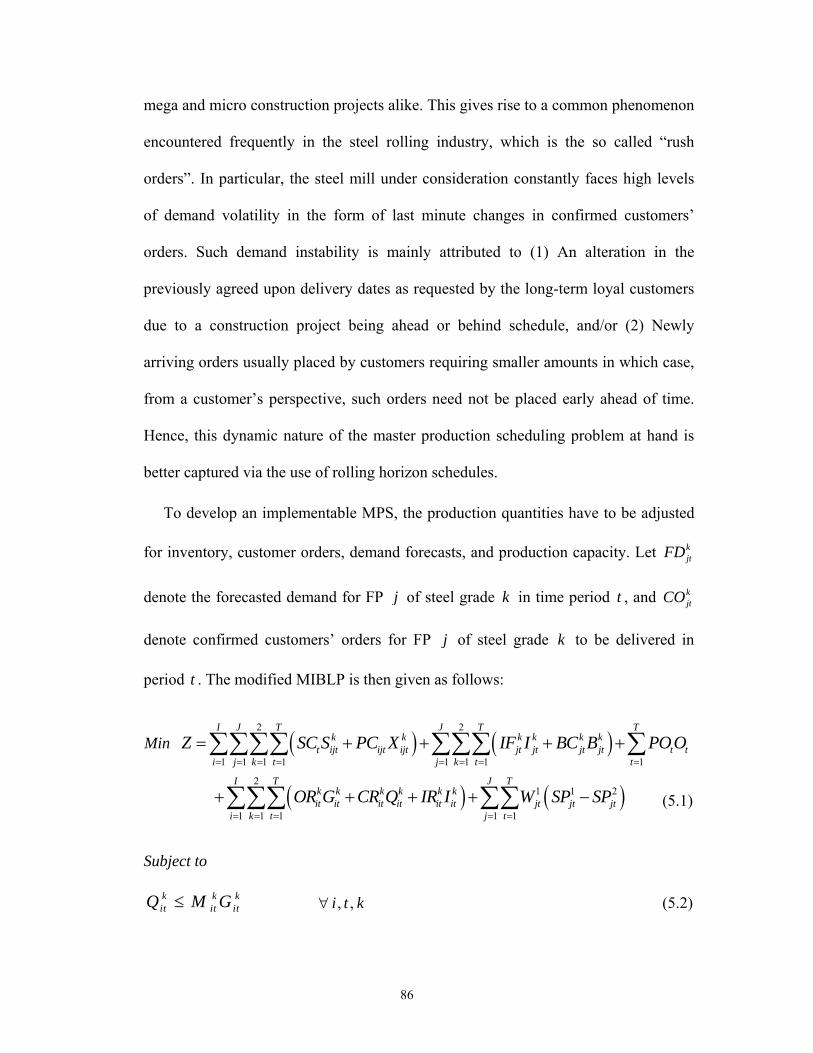
86
mega and micro construction projects alike. This gives rise to a common phenomenon
encountered frequently in the steel rolling industry, which is the so called “rush
orders”. In particular, the steel mill under consideration constantly faces high levels
of demand volatility in the form of last minute changes in confirmed customers’
orders. Such demand instability is mainly attributed to (1) An alteration in the
previously agreed upon delivery dates as requested by the long-term loyal customers
due to a construction project being ahead or behind schedule, and/or (2) Newly
arriving orders usually placed by customers requiring smaller amounts in which case,
from a customer’s perspective, such orders need not be placed early ahead of time.
Hence, this dynamic nature of the master production scheduling problem at hand is
better captured via the use of rolling horizon schedules.
To develop an implementable MPS, the production quantities have to be adjusted
for inventory, customer orders, demand forecasts, and production capacity. Let kjtFD
denote the forecasted demand for FP j of steel grade k in time period t , and kjtCO
denote confirmed customers’ orders for FP j of steel grade k to be delivered in
period t . The modified MIBLP is then given as follows:
( ) ( )
( ) ( )
2 2
1 1 1 1 1 1 1 1
21 1 2
1 1 1 1 1
I J T J T Tk k k k k k
t ijt ijt ijt jt jt jt jt t ti j k t j k t t
I T J Tk k k k k kit it it it it it jt jt jt
i k t j t
Z SC S PC X IF I BC B POO
OR G CR Q IR I W SP SP
= = = = = = = =
= = = = =
= + + + +
+ + + + −
∑∑∑∑ ∑∑∑ ∑
∑∑∑ ∑∑
Subject to
k k kit it itQ M G≤ , ,i t k∀ (5.2)
(5.1)
Min

87
2
1 1 1
1I J
kijt
i j k
Sb= = =
=∑∑∑ t∀ (5.3)
'2' , 1 '
' , 1' 1 1 ' 1 '
0.4 24kI Ji j tk k k k
ijt ijt i j t ij ijti j k i j
XS Sb S ST Sd
α′ −
′ −′= = = ′
⎛ ⎞⎛ ⎞⎛ ⎞⎜ ⎟= × − + + ×⎜ ⎟⎜ ⎟⎜ ⎟⎜ ⎟⎜ ⎟⎝ ⎠⎝ ⎠⎝ ⎠
∑∑∑ , , ,i j t k∀ (5.4)
2
1 1 1
kI Jijt k
ijt t ti j k ij
XS A O
α= = =
⎛ ⎞+ ≤ +⎜ ⎟⎜ ⎟
⎝ ⎠∑ ∑ ∑ t∀ (5.5)
t otO A≤ t∀ (5.6)
( )k k kijt t ijt ijt ijX b Sb Sd ρ= × + × , , ,i j t k∀ (5.7)
, 11
Jk k k k kit i t it t ijt ijt
jI I Q b Sb Sd−
=
⎡ ⎤= + − × +⎣ ⎦∑ , ,i t k∀ (5.8)
{ }1 1 1 1 1 1 1 1, , , 1 , 1
1,
I
j t j t j t j t ijt jt jt jti
I B I B X W Max FD CO− −=
− = − + − −∑ ,j t∀ (5.9)
{ }2 2 2 2 2 2 1 2 2, , , 1 , 1
1
,I
j t j t j t j t ijt jt jt jt jti
I B I B X W W Max FD CO− −=
− = − + − + −∑ ,j t∀ (5.10)
0 0 0k k kj j jTI B B= = = ,j k∀ (5.11)
, , , , , , , 0k k k k k k kijt it ijt t jt it jt jtSd Q X O W I I B ≥ , , ,i j t k∀ (5.12)
{ }, 0,1k kit ijtG Sb ∈ , , ,i j t k∀ (5.13)
kijtSd N∈ , , ,i j t k∀ (5.14)
The inventory balance constraints in the model are adjusted for the maximum
value of customers’ orders and demand forecasts as seen in Equations (5.9) and
(5.10). In the remainder of this chapter, the above model is referred to as the exact
model, or the full scale model. The next section presents approximate models which
provide a quick remedy to the challenging and time consuming task associated with

88
the repetitive solution of the exact model to optimality as new values for problem
parameters become available.
5.5 Approximate rolling horizon models
Due to the uncertainties involved, solving the exact model at the beginning of the
first period and freezing the resulting MPS for the entire planning horizon (i.e.,
implementing the MPS all the way) will most certainly produce poor quality
solutions. Alternatively, the decision maker is better off implementing only the first
period’s decisions and then rolling the horizon forward before implementing the
second period’s decisions in light of the newly available data, and so on. Under the
proposed scenario, the decisions associated with the most immediate time period are
made based on the confirmed customers’ orders. On the other hand, for the
unimplemented portion of the cycle, production is planned according to the maximum
of forecasted demand and confirmed orders, where both of these quantities are
updated periodically as the horizon rolls forward. Such decision making criterion for
a planning horizon of 4T = is depicted in Figure 5.2, where ( 1)kjtFD t − and
( 1)kjtCO t − denote demand forecasts and confirmed orders at the end of period 1t − ,
respectively. The dashed line box in the figure indicates the implemented master
production schedule. In this policy, changes in the actual rolled bars selling prices and
billets purchasing prices are also accounted for as the horizon rolls forward.
Following the proposed rolling horizon scheme, the exact model is re-solved at
the beginning of each period and the production decisions are updated accordingly.
However, due to complexities associated with solving the exact model to optimality,

89
the process of frequently re-solving such model consumes an impractical amount of
computational time. As such, three families of approximate models, which only
generate exact schedules for the immediate time periods, are developed. The basic
idea behind such approximation is that the key complicating aspects of the exact
model, which prevent the attainment of quick solutions such as major setup time and
minimum batch size restriction, are relaxed only for future time periods.
Figure 5.2: The employed rolling horizon strategy
As pointed out by Clark and Clark (2000), plant schedulers far prefer models that
make decisions quickly since many scenarios, usually concerning demand forecast
and machine availability, often have to be evaluated with what-if analysis before a
final decision is made. In addition, it is difficult to obtain precise estimates for the
1t =
{ }(0), (0)k kjt jtMax FD CO
2t = 3t = 4t =
1(0)kjCO
Roll forward
Roll forward{ }(1), (1)k kjt jtMax FD CO
3t = 4t = 5t =
2 (1)kjCO
2t =
5t = 6t =
3 (2)kjCO
3t = 4t =
{ }(2), (2)k kjt jtMax FD CO
7t =
4 (3)kjCO
4t = 5t = 6t =
{ }(3), (3)k kjt jtMax FD CO
Roll forward

90
backlogging cost since it is highly dependent on the market conditions and the
importance of the customer. As such, the values used for such cost are usually based
on subjective judgment and vague information. Hence, instead of solving the exact
model optimally which often requires substantial computational efforts and achieves
only limited added value, the decision maker would rather make use of smaller
alternative models that can provide faster responses without big losses in the quality
of the decisions made.
In this section, we seek to resolve the excess computational time, associated with
obtaining the optimal solution to the exact model, via proper relaxation of the
complicating variables and/or constraints, resulting in a reduced problem size
dimensionality and great savings in computational efforts. Only those approximate
models that generate exact schedules for the most immediate time period are
considered. Hence, the relaxations are only applied to the unimplemented time
periods of the planning horizon. Three varieties of alternative models are considered,
where each model targets a certain complicating aspect of the exact model. The
quality of the schedules obtained from applying these models is benchmarked against
one another and against those of the exact model, where the last comparison is only
possible for small problems that are optimally solvable in feasible computing time.
Since the analysis is carried out on a rolling schedule basis which requires the
repetitive solution of the model, our work shall provide the decision maker with
practical and more efficient alternatives towards the quick attainment of good quality
solutions (i.e. within the proximity of those obtained through solving the exact

91
model). Although the generated solutions might be sub-optimal, they still provide
substantial improvement on intuitive or indeed rule-generated production schedules.
In general, for a rolling horizon policy that calls for implementing the decisions
concerning, say, the first τ periods, Clark and Clark (2000) were the first to address
questions like: Is it necessary to have 0/1 solution values for the binary setup
variables in the last T τ− periods (i.e., the unimplemented portion of the planning
horizon)? Why not reduce the number of 0/1 variables by representing the setups for
the last T τ− periods as relaxed continuous variables between 0 and 1? They also
argue that even more computing time is economized by eliminating the binary setup
variables from the last T τ− periods. This removal is compensated for by increasing
the values of the unit production times to take the setup times into account. Their
argument is backed up by an established fact in the literature (e.g., Trigeiro et al.
1989) which demonstrates the noticeable increase in models complexity once the
setup times are explicitly accounted for.
Looking back at the exact model at hand, it is observed that the binary variables
concerning the major setup time, kijtSb , induce bilinearity and hence prevent the direct
attainment of quick solutions except via classical linearization approaches that have
doubtable efficiency. This fact motivates the relaxation of the binary restriction
(constraint 5.13) on these kijtSb variables only for the unimplemented periods in which
those variables may now assume a continuous value between 0 and 1. In our case,
such a relaxation would greatly reduce the number of 0/1 kijtSb variables (from
I J T K× × × to I J K× × ) and is expected to save on the solution time. This
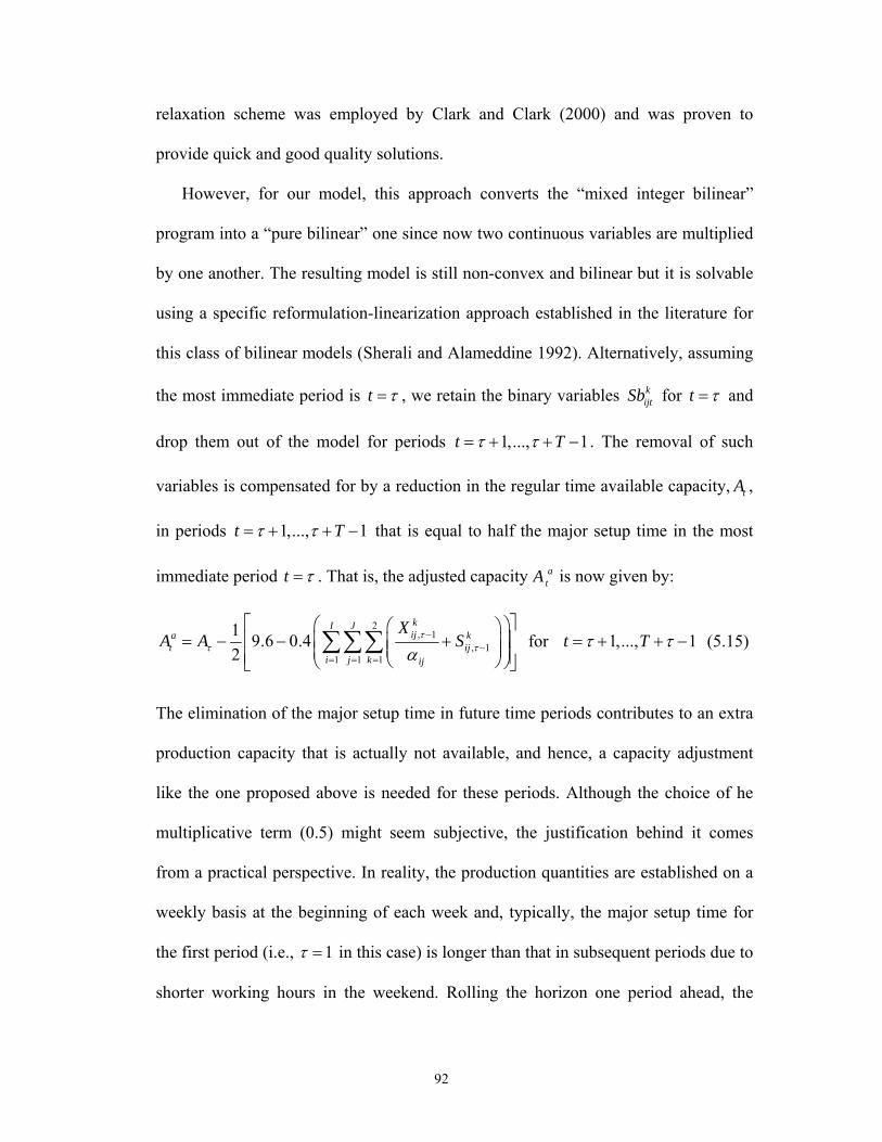
92
relaxation scheme was employed by Clark and Clark (2000) and was proven to
provide quick and good quality solutions.
However, for our model, this approach converts the “mixed integer bilinear”
program into a “pure bilinear” one since now two continuous variables are multiplied
by one another. The resulting model is still non-convex and bilinear but it is solvable
using a specific reformulation-linearization approach established in the literature for
this class of bilinear models (Sherali and Alameddine 1992). Alternatively, assuming
the most immediate period is t τ= , we retain the binary variables kijtSb for t τ= and
drop them out of the model for periods 1,..., 1t Tτ τ= + + − . The removal of such
variables is compensated for by a reduction in the regular time available capacity, tA ,
in periods 1,..., 1t Tτ τ= + + − that is equal to half the major setup time in the most
immediate period t τ= . That is, the adjusted capacity atA is now given by:
2, 1
, 11 1 1
1 9.6 0.42
kI Jija k
t iji j k ij
XA A Sτ
τ τα−
−= = =
⎡ ⎤⎛ ⎞⎛ ⎞⎢ ⎥= − − +⎜ ⎟⎜ ⎟⎜ ⎟⎜ ⎟⎢ ⎥⎝ ⎠⎝ ⎠⎣ ⎦
∑∑∑ for 1,..., 1t Tτ τ= + + − (5.15)
The elimination of the major setup time in future time periods contributes to an extra
production capacity that is actually not available, and hence, a capacity adjustment
like the one proposed above is needed for these periods. Although the choice of he
multiplicative term (0.5) might seem subjective, the justification behind it comes
from a practical perspective. In reality, the production quantities are established on a
weekly basis at the beginning of each week and, typically, the major setup time for
the first period (i.e., 1τ = in this case) is longer than that in subsequent periods due to
shorter working hours in the weekend. Rolling the horizon one period ahead, the

93
ending inventory levels for RM and FP, the demand forecasts and confirmed orders,
the selling and purchasing prices are updated after each period. The resulting model is
a MILP that is directly solvable using off-the-shelf optimization packages such as
AMPL/CPLEX. This model will be referred to as model ARH in the remainder of this
chapter.
The second approximate model, called BRH, addresses another source of
complexity in the exact model arising from the integrality restriction on the variables
kijtSd (constraint 5.14). Recall that these variables denote the number of minor setups,
or equivalently the number of batches produced after the initial batch, where the
furnace capacity restricts the size of each batch to 60 tons each, which better complies
with the economies of scale principles. As established earlier, lot-sizing rules are one
of the design factors when it comes to developing MPS on a rolling horizon basis. As
such, this model eliminates the restriction of minimum batch size production through
relaxing the integrality restriction on the kijtSd variables (i.e., allowing the production
of partial batches) for the unimplemented time periods only (i.e.
1,...., 1t Tτ τ= + + − ). This allows for a better understanding of how lot-sizing rules
impact the total cost in rolling horizon schedules. For the kijtSd variables to assume
continuous values, they need to be redefined as follows:
kijtSd : Quantity of batches of FP j produced from RM i both having steel grade k
conducted during period t (i.e. after producing the first batch).
To serve for better approximation purposes, the setup time expression (Equation
5.4) for periods 1,...., 1t Tτ τ= + + − would still be calculated based on integral

94
number of batches. In reality, a minor setup takes place between each batch produced
and the time for this setup is independent of the batch size. Therefore, the updated
expression for the setup time in this case is given by:
'' , 1 '
' , 1' ' '
0.4 24kIi j tk k k k
ijt ijt i j t ij ijti j k i j
XS Sb S ST Sd
α′ −
′ −′ ′
⎛ ⎞⎛ ⎞⎛ ⎞⎜ ⎟= × − + + ×⎜ ⎟⎜ ⎟⎜ ⎟⎜ ⎟⎜ ⎟⎝ ⎠⎝ ⎠⎝ ⎠
∑ , , ,i j k t τ∀ = (5.16)
'' , 1 '
' , 1' ' '
0.4 24kIi j tk k k k
ijt ijt i j t ij ijti j k i j
XS Sb S ST Sd
α′ −
′ −′ ′
⎛ ⎞⎛ ⎞⎛ ⎞⎜ ⎟ ⎡ ⎤= × − + + ×⎜ ⎟⎜ ⎟ ⎢ ⎥⎜ ⎟⎜ ⎟⎜ ⎟⎝ ⎠⎝ ⎠⎝ ⎠
∑
, , , 1,..., 1i j k t Tτ τ∀ = + + − (5.17)
where kijtSd⎡ ⎤⎢ ⎥ denotes the smallest integer greater than or equal to k
ijtSd . Note that the
resulting model is still a MIBLP since the binary variables kijtSb were retained for all
time periods in this model. As such, adopting the classical linearization scheme of
Glover (1975), the following sets of constraints overcome the existent bilinearity and
replace the above constraints of (5.16) and (5.17):
9.6 0.4k k k kijt ijt ijt ij ijtS Sb y ST Sd= × − × + × , , ,i j k t τ∀ = (5.18)
9.6 0.4k k k kijt ijt ijt ij ijtS Sb y ST Sd⎡ ⎤= × − × + × ⎢ ⎥ , , , 1,..., 1i j k t Tτ τ∀ = + + − (5.19)
k k k k kijt ijt ijt ijt ijtL Sb y U Sb≤ ≤ , , ,i j t k∀ (5.20)
( ) ( )' '
' , 1 ' , 1' '' , 1 ' , 1
' ' ' '' '
1 1k ki j t i j tk k k k k k k
i j t ijt ijt ijt i j t ijt ijti j k i j ki j i j
X XS U Sb y S L Sb
α α′ ′− −
′ ′− −′ ′′ ′
⎛ ⎞ ⎛ ⎞+ − − ≤ ≤ + − −⎜ ⎟ ⎜ ⎟⎜ ⎟ ⎜ ⎟
⎝ ⎠ ⎝ ⎠∑ ∑
, , ,i j t k∀ (5.21)
Clearly, the resulting linearized version of the model is now readily solvable using
AMPL/CPLEX 11.0.

95
In the above analysis, model ARH tackles the binary restriction on the kijtSb
variables while model BRH tackles the integrality restriction on the kijtSd variables
without touching the kijtSb variables. This quantifies the quality of the solutions as
well as the savings in computational time obtained using each approximation criterion
separately. Towards achieving even further savings in the computational time, the
approximation schemes adopted in models ARH and BRH are combined. Hence, this
hybrid model, called CRH, contains no kijtSb variables in the periods
1,...., 1t Tτ τ= + + − and assumes that the kijtSd variables are continuous during those
periods as well. However, for the most immediate period t τ= , all of the full scale
model constraints are retained so that only exact schedules are generated.
5.6 Computational experiments
The purpose of this section is to provide insights into the performance of the
proposed models in terms of the quality of solutions obtained (i.e., closeness of the
objective function value obtained via approximations to that of the exact model),
savings in computational time and reduction in problem dimensionality. To ensure a
fair comparison, ten problem instances of different sizes are tested and each model is
solved under the same set of input parameters. All models were coded using AMPL
programming language (Fourer et al. 2003) and solved using CPLEX 11.0 solver,
where the solver option is set to solve integer problems using the built-in branch and
cut algorithm. The values for the different input parameters are generated within
certain range of intervals, as shown in Table 5.1.

96
Table 5.1: Selected range of values for input parameters in the test problems
Input parameter Range of values Input parameter Range of values kitCR (500 , 800) k
jtBC (20 , 35) kitOR (2000 , 2200) k
jtSP (1300 , 1700) kitIR (10 , 20) k
itM (150 , 300)
ijtPC (15 , 35) ijρ (0.80 , 0.95)
tPO (300 , 500) ijα (50 , 58)
tSC (600 , 800) kjtFD , k
jtCO (0 , 100) kjtIF (15 , 30) ijST (0.25 , 1.0)
It should be noted that all models are applied dynamically on a rolling horizon
basis in which only the first period’s outcome contributes to the total cost function. In
other words, the reported results are for the implemented plans and, as such, the
comparison is only made between exact schedules generated through the different
models. The objective is to study the effect of the relaxations made to future (i.e.,
unimplemented) time periods on the current period’s decisions. Under such a rolling
horizon policy, the results of the current period establish the next periods’ major setup
time (if any), and the initial levels of RM inventory, FP inventory and backlog record
for the next run. In addition, before rerunning the model, any encountered changes in
the values of the problem parameters, mainly demand forecasts and customers’ orders
are updated in the model. The obtained results for the exact model, for those instances
solvable within feasible computational time, along with the three approximate ones
are reported in Tables 5.2-5.5 below. Note that the solution time indicates the total
time it takes to solve the model T times, and the total cost is the one resulting from
the implemented plans. The reported number of variables and constraints for the exact

97
model as well as model BRH are for the linearized version of those models, while
these numbers are for the reduced size MILP in case of models ARH and CRH.
Table 5.2: Obtained numerical results for the exact model
Values of Indices Problem
Instance I J T K
No. of Variables
No. of Constraints
Solution time (sec) Total Cost
1 1 2 2 2 74 140 0.95 778,368
2 1 3 3 2 159 297 2.48 1,112,105
3 2 3 3 2 267 507 8,289 1,151,720
4 2 3 4 2 358 678 33,694 1,542,301
5 3 4 4 2 644 1,232 * *
6 4 4 4 2 828 1,592 * *
7 4 5 4 2 1,010 1,946 * *
8 5 5 4 2 1,234 2,386 * *
9 5 6 4 2 1,456 2,820 * *
10 5 7 5 2 2,101 4,071 * *
*Code execution was interrupted after 12 hours of run time with no results obtained. Table 5.3: Obtained numerical results for model ARH
Values of Indices Problem
Instance I J T K
No. of Variables
No. of Constraints
Solution time (sec) Total Cost
1 1 2 2 2 62 111 0.94 778,368
2 1 3 3 2 129 229 3.73 1,077,312
3 2 3 3 2 207 373 9.04 1,127,154
4 2 3 4 2 274 495 57.27 1,520,070
5 3 4 4 2 476 869 600.41 1,588,562
6 4 4 4 2 604 1,109 7,855 1,445,971
7 4 5 4 2 730 1,343 9,249 1,723,936
8 5 5 4 2 884 1,633 16,154 1,687,157
9 5 6 4 2 1,036 1,917 29,373 1,721,446
10 5 7 5 2 1,471 2,737 41,069 2,279,638

98
Out of the four solvable test problems for the exact model, better proxies are achieved
via model ARH (instances 1, 3 and 4) while models BRH and CRH provide for a
better approximation as for the second problem instance. In particular, the worst
deviation, in terms of objective function value, among all models is not more than
3.65% under tight capacity conditions.
Table 5.4: Obtained numerical results for model BRH
Values of Indices Problem
Instance I J T K
No. of Variables
No. of Constraints
Solution time (sec) Total Cost
1 1 2 2 2 78 143 0.82 776,051
2 1 3 3 2 165 295 1.40 1,095,979
3 2 3 3 2 279 505 2.73 1,109,694
4 2 3 4 2 370 663 11.83 1,504,809
5 3 4 4 2 668 1,205 108.33 1,567,408
6 4 4 4 2 860 1,557 2,915 1,419,194
7 4 5 4 2 1,050 1,903 2,602 1,723,807
8 5 5 4 2 1,284 2,333 6,274 1,687,766
9 5 6 4 2 1,516 2,757 15,007 1,706,723
10 5 7 5 2 2,171 3,927 27,838 2,279,037
If we are to benchmark the values of the approximate models’ total cost against
one another for all test problems, there exists a maximum of 3.44% deviation for
problem instance number 6. However, for situations where there is abundant capacity
available (i.e. total demand << capacity), one would expect all models to produce
very similar, if not exactly the same, production schedules. This is due to the fact that,
under low demand scenario, the model actually has less number of non-zero decision
variables to optimize since backlogged quantities, overtime hours and substitution
quantities are all set to zero.

99
Table 5.5: Obtained numerical results for model CRH
Values of Indices Problem
Instance I J T K
No. of Variables
No. of Constraints
Solution time (sec) Total Cost
1 1 2 2 2 66 115 0.80 764,689
2 1 3 3 2 135 229 1.22 1,095,979
3 2 3 3 2 219 373 1.26 1,116,810
4 2 3 4 2 286 483 1.77 1,514,967
5 3 4 4 2 500 845 1.81 1,549,973
6 4 4 4 2 636 1,077 1.81 1,396,213
7 4 5 4 2 770 1,303 1.83 1,723,856
8 5 5 4 2 934 1,583 2.08 1,686,208
9 5 6 4 2 1,096 1,857 2.30 1,674,332
10 5 7 5 2 1,541 2,597 4.09 2,278,262
From a solution time perspective, major benefits are obtained through making use
of the approximate models instead of the exact one without, as just illustrated,
compromising the quality of such solutions. By comparing the times for models ARH
and BRH, we notice that more computational time savings are attained from applying
model BRH (up to 81.96% reduction for instance No. 7). This shows that the
minimum batch size restriction associated with the kijtSd variables (i.e., integrality
restriction) contributes a lot more to the complexity of the exact model, hence greatly
limiting its applicability, as compared to the binary restriction on the variables kijtSb . It
is obvious that since model CRH combines the relaxations employed in the other two
approximate models, it would result in substantial savings in computational time. For
example, it took the exact model 33,694 seconds (9.36 hours) to solve problem
instance No. 4 while model CRH solved it in less than two seconds with a difference

100
in the total cost of only 1.77%. For a larger problem size ( 5I T= = , 7J = and 2K = )
the solutions to the exact model are not attainable within 12 hours of computational
time, while such problem is solved via model CRH within 4 seconds only.
If the models were to be implemented on a static horizon basis, one knows that
model CRH provides a lower bound for both models ARH and BRH which in turn
would yield a lower bound on the objective function value of the exact model.
However, rolling horizon outcomes are usually different from static horizon ones and,
as such, relaxing some of the constraints for the unimplemented time periods does not
necessarily guarantee a lower objective function value for the more restricted model
once both models are applied on a rolling horizon basis and the implemented plans
are compared. As a matter of fact, model ARH results in a lower total cost for
problem instance No. 2 as compared to that obtained from model CRH. In addition, in
4 out of the 10 test problems, model BRH yield a total cost that is lower than that of
model CRH.
5.7 Summary
This chapter has dealt with the master production scheduling problem in steel
rolling mills operating in an environment of dynamic demand. The problem was
formulated as a mixed integer bilinear program, in which both forecasted demand and
confirmed customers’ orders are incorporated. To better capture the existent volatility
in demand, the developed model was implemented on a rolling horizon basis where
the values for the forecasts and orders, among other problem parameters, were
updated every period in light of the newly available information obtained form the

101
market. As the developed production schedule is only implemented for the most
immediate time period, production and inventory related decisions for this period
were based on the actual orders received.
Since solving the exact model to optimality turns out to be a challenging task, the
alternative approach of dealing with approximate models is adopted. Three variants of
such models were developed where each of these models tackles the sources of
complexity associated with the exact model, either one at a time or both at once,
resulting in smaller models with a tractable number of binary and/or integer variables.
Based on numerical experiments for several test problems, it is observed that such
approximate models are particularly efficient and thus have a great potential in
production planning problems where optimal solutions to full scale mathematical
models are not quickly attainable. Hence, a fair compromise between the quality of
the solutions and substantial computational time savings is achieved via the
employment of these approximate models.
102
Chapter 6
Modeling Demand Uncertainty in Production Planning
through Fuzzy Set Theory Approach
6.1 Introduction
Fuzzy set theory (FST) is a theory of graded concepts (a matter of degree), but not
a theory of chance (Lai and Hwang 1992a). It allows for the development of more
robust and flexible models that better capture the human aspects involved in real
world complex systems. In general, FST represents an attractive tool to aid research
in production management when the dynamics of the production environment limit
the specification of model objectives, constraints and the precise measurement of
model parameters (Guiffrida and Nagi 1998). Unlike the rolling horizon approach
adopted in the previous chapter, the utilization of FST alleviates the necessity for
repeatedly solving the model at the beginning of each time period. In general, there
exist several advantages to the utilization of FST to handle such type of uncertainties:
(1) It generally allows for the transformation of qualitative estimates that are
expressed linguistically based on human perception into exact quantitative values,
expressed in terms of fuzzy sets.
103
(2) It provides for a broader alternative to account for uncertainty as compared to the
classical approach that utilizes probability distributions. When there is a lack of
evidence or lack of certainty in evidence, the standard probabilistic reasoning
methods are not appropriate (Petrovic and Petrovic 1999).
(3) From a mathematical programming perspective, fuzzy models overcome the
rigid requirements characterizing standard deterministic models. This greatly
facilitates the decision making process in most real life applications where the
determination of the exact model parameters poses a crucial practical challenge.
(4) Obtaining an initial compromise solution from the fuzzy model allows the
decision maker to specify which further information should be obtained to improve
the solution. This procedure obviously offers the possibility to limit the acquisition
and processing of information to the relevant components and therefore information
costs will be distinctly reduced (Rommelfanger 1996).
(5) The fuzzy models provide decision makers with some flexibility to incorporate
their own priority into the model through the selection of aspiration levels (in the case
of a fuzzy objective function) and the tolerance interval. As such, alternative decision
plans corresponding to different degrees of satisfaction are easily attainable.
In this chapter, the vagueness and impreciseness associated with the estimation of
future demand figures is captured through the use of FST, originally introduced in the
seminal work of Zadeh (1965). In addition, we clearly establish the difference
between the two approaches used to handle fuzzy quantities in mathematical models,
namely flexible mathematical programming (FMP) and possibilistic programming
(PP), since such distinction has never been made solid in the literature. We then adopt
104
the FMP approach to handle uncertainties in demand through expressing the demand
constraint as a flexible one. Our objective is to emphasize on the superiority of this
approach for modeling production planning problems and illustrate the economic
benefits obtained through the use of fuzzy models as compared to traditional
deterministic models. To facilitate understanding the analysis presented in this
chapter, some basic FST related background needs to be established first.
6.2 A brief introduction to fuzzy set theory
In classical set theory, the relation between an object x and the ordinary set of
objects A is defined by the characteristic function or the indicator function as follows:
1( )
0A
if x Ax
if x A∈⎧
ϒ = ⎨ ∉⎩ (6.1)
Hence, a member either belongs or does not belong to a particular set. Fuzzy set
theory, however, simulates the actual practice and allows for a member to belong to
different sets with various degrees of membership. The following formal definitions
are based on the work of Rommelfanger (1996) and Demirli (2005).
Definition 6.1: Let X denote the universal set (also referred to as the universe of
discourse), then the set of ordered pairs:
( ){ }, ( ) | ,AA x x x Xμ= ∈ where [ ]: 0,1A Xμ → (6.2)
is called a fuzzy set in X . The function ( )A xμ is called the membership function
which establishes the grade of membership of element x in A .
Definition 6.2: Let A be a fuzzy set in X . The support of A , denoted by supp(A), is
the crisp set of X whose elements have nonzero membership grades in A :

105
supp(A) = { }| ( ) 0Ax X xμ∈ > (6.3)
The core of A , denoted by core(A), is the crisp set of X whose elements have a
membership grade in A equals to one:
core(A) = { }| ( ) 1.0Ax X xμ∈ =
The height of A , denoted by h(A), is the largest membership grade obtained by any
element in that set:
h(A) = sup ( )Ax X
xμ∈
(6.4)
Definition 6.3: A fuzzy set A is called normal when ( ) 1h A = ; it is called subnormal
when ( ) 1h A < .
Definition 6.4: A fuzzy set A in a convex set X is called convex if:
( ) ( )1 2 1 2(1 ) ( ), ( ) ,A A Ax x Min x xμ λ λ μ μ+ − ≥ 1 2, ,x x X∈ [ ]0,1λ ∈ (6.5)
Definition 6.5: A convex normalized fuzzy set ( ){ }, ( ) |AA x x x Rμ= ∈ on the real
line R such that:
(I) there exist exactly one 0x R∈ with the membership degree 0( ) 1,A xμ = and
(II) ( )A xμ is piecewise continuous in ,R
is called a fuzzy number.
Definition 6.6: (Fuzzy Decision making of Bellman and Zadeh (1970)
Let X be the set of alternatives, which defines the set to all possible solutions to a
decision problem. The fuzzy goal G and a fuzzy constraint C are fuzzy sets on
X and characterized by their respective membership functions [ ]: 0,1G Xμ → and
[ ]: 0,1C Xμ → . Then, G and C combine to form a decision, D , which is a fuzzy set

106
resulting from the intersection of G and C (i.e., D G C= ∩ ). The fuzzy decision set
is characterized by its membership function:
( ) ( ) ( ) ( ( ), ( ))D G C G Cx x x Min x xμ μ μ μ μ= ∧ = (6.6)
and the corresponding maximizing decisions can then be defined as:
( ) ( ( ), ( ))D G CMax x MaxMin x xμ μ μ= (6.7)
It should be noted that definition 7.6 requires the assumption of symmetry to be
satisfied in order to reach decisions that satisfy both the goal “and” the constraint.
6.3 Flexible mathematical programming (FMP) vs. possibilistic
programming (PP)
There are two approaches that researchers use in order to deal with fuzzy
mathematical models where the suitability of the chosen approach depends on the
nature of the existent fuzziness in the model. The two approaches are flexible
mathematical programming (FMP), in which the rigidity restriction on the
comparison operator (i.e., equality or inequality operators) is relaxed resulting in a
soft or flexible set of constraints, and possibilistic programming (PP), in which the
imprecise coefficients are expressed as fuzzy numbers having a specified possibility
distribution. We distinguish between these two approaches in the general context of
fuzzy mathematical programming before applying such distinction to the model at
hand. It is of great importance to understand this distinction while modeling
fuzziness/imprecision in mathematical programming problems.
Flexibility is modeled by fuzzy sets and may reflect the fact that constraints or
goals are linguistically formulated; their satisfaction is a matter of tolerance and

107
degrees or fuzziness (Mula et al. 2006). FMP utilizes subjective preference-based
membership functions where these functions are constructed by eliciting the
preference information from the decision makers. In this scenario, the membership
function is equivalent to the utility function when the membership functions of FMP
are based on a preference concept like the utility theory (Lai and Hwang 1992a).
Hence, the grade of a membership function indicates a subjective degree of the
decisions maker’s satisfaction within given tolerances. Clearly, the characteristic
function in FMP is a membership function. Applications of FMP approach can be
found in Pendharkar (1997), Miller et al. (1997), Itoh et al. (2003) and Mula et al.
(2006).
On the other hand, possibility theory is adopted in situations where the model
parameters are imprecise due to uncertainty in the data or lack of knowledge (i.e.
epistemic uncertainty). It is noted that the possibility measure of an event might be
interpreted as the possibility degree of its occurrence under a possibility distribution;
an analogous to - yet different from - probability distribution (Lai and Hwang 1992a).
In essence, an important difference between the probability theory and the possibility
theory is that the sum of probabilities for all possible outcomes should be equal to
one, while the sum of possibilities for all possible events under possibility theory
need not be equal to one. Hence, the possibility distribution is constructed by
considering the possible occurrence of events where the grade of possibility indicates
the subjective or objective degree of a particular event occurring. Clearly, the
characteristic function in PP is a possibility distribution. PP has also been widely
108
applied to various problems as can be seen in Liang (2007), Demirli and Yimer
(2008), Liang (2008), and Yimer and Demirli (2009).
In general, possibility theory would be adapted to uncertain situations in which
the demand is fuzzy due to lack of information, and is represented by a fuzzy number,
but the demand constraint still holds as a strict (in)equality. As such, once the demand
has been defuzzified, the resulting crisp constraint holds as a rigid requirement and
the decision maker has no choice but to seek a solution that fully satisfies such
constraint. On the other hand, flexible mathematical programming deals with
situations involving either fuzzy or crisp demand but the corresponding constraint is
rather flexible. Therefore, the existent flexibility within the model allows for
“approximate” fulfillment of the demand, chosen subjectively according to the
decision maker’s preference, which indicates that the comparison operator is being
treated as a fuzzy relationship.
Turning back to the problem at hand, the model developed in this chapter
determines the daily/weekly production lot sizes and serves for short-term planning
purposes. However, the fuzzy nature of the demand in the form of last minute orders,
called “rush orders”, still raises a major concern to the decision maker. For an
essential material such as steel bars, the realized demand in a particular time period
could be greater or less than the confirmed orders established at the beginning of the
planning horizon. While the former case is mainly attributed to a collection of small
magnitude orders usually placed by short term customers, the latter is due to an
alteration on a short notice of a previous order typically placed by long term
customers. Depending on the magnitude of such orders, they could cause major

109
disruptions to the production system which induces a high associated cost. Hence, it
seems only logical to allow some degree of flexibility into the mathematical model so
that it possesses the ability to whether satisfy all orders or only some orders while
completely ignoring some other ones, whichever option deems more profitable. By
treating the demand constraint as flexible rather than a rigid one, the emphasis now is
on to which extent the demand shall be met instead of enforcing a strict policy of
being 100% responsive to a fluctuating customer demand. This resembles the actual
situation where the decision maker has the choice to accept, reject or partially fulfill
an order as soon as it arrives. A good practical example is the famous Japanese
automaker Company “Nissan” which faces a highly fluctuating demand and deals
with it through ignoring some of the orders since such fluctuations are costly to meet.
In the fuzzy model presented in Section 6.5, we mimic the decision maker’s ability to
reject or accept rush orders, whether partially or fully, through representing the
flexible demand constraints by fuzzy sets having triangular membership functions
(TMFs). The allowable deviations from the most likely value are expressed as
percentages of the confirmed orders.
6.4 Fuzzy mathematical programming
The uncertainties associated with the operating environment of the steel mill
under consideration necessitate the use of FST to explicitly account for the dynamic
nature of the problem. In general, whenever FST is employed in the context of
mathematical programming, the decision maker is faced with important factors that
need to be carefully addressed towards a better representation of the problem at hand:

110
(1) Sources of uncertainty: Depending on the problem, it might be difficult to obtain
precise estimates for certain problem parameters such as cost coefficients, supply and
demand quantities, machine capacities and supplier lead time. In essence, one has to
establish what exactly is fuzzy about the problem at hand before anything else.
(2) Representation of fuzziness: As discussed earlier, accommodating for fuzzy
quantities in the context of mathematical programming is accomplished through the
use of flexible programming or possibilistic programming depending on the nature of
the existent fuzziness associated with the parameters of concern.
(3) Form of membership functions: This involves defining the support of the
membership function as well as the form of the function over the identified interval.
There exist several propositions for modeling the membership function including
monotonic linearly increasing or decreasing, piecewise linear, triangular or
trapezoidal, concave shape or s-shape (Rommelfanger 1996).
(4) Aggregation operators (aggregators): In analogy to the deterministic
mathematical programming case, a fuzzy decision set is reached at through
aggregating the membership functions of the fuzzy objective function and constraints.
Such aggregation is achieved through several operators that have been well
established in the literature (e.g., Bellman and Zadeh 1970, Werners 1988 and
Zimmerman and Zysno 1980).
While the approach of flexible mathematical programming (FMP), which seems
to be more efficient computationally (Zimmermann 2001), has been successfully
applied by several authors, the vast majority have adopted linear membership
functions throughout their work since such form is computationally efficient and
111
entails a reduced dimensionality for the resulting equivalent crisp model (e.g.,
Pendharkar 1997, Miller et al. 1997, Itoh et al. 2003). However, for a better
resemblance of reality, we believe that the flexible demand constraint is better
represented by a fuzzy set having a triangular membership function (TMF).
In the context of FMP, there are two classes of models: symmetric and non-
symmetric models. The symmetric models are based on the definition of a fuzzy
decision originally proposed by Bellman and Zadeh (1970) in which they assume that
objective(s) and constraint(s) are an ill-structured situation and can be represented by
fuzzy sets. These models involve less computational effort and are thus easier to
handle since a decision can be readily stated as the confluence of the fuzzy
objective(s) and fuzzy constraint(s). However, they suffer from two shortcomings.
First, the interval of allowance (i.e., support) of the fuzzy set representing the
objective function should be given initially. As such, this interval is usually decided
upon blindly based on a purely subjective judgment obtained from the decision
maker. Secondly, requiring the initial determination of such interval pays little or no
attention to the decision maker’s preference on the degree of flexibility of the
respective fuzzy constraints. As pointed out by Lai and Hwang (1992a), in real world
problems, it is unrealistic to initially ask the decisions maker to give this interval
without providing any information about it. For these models, Zimmerman (1976)
was the first to confirm the existence of an equivalent ordinary linear program
through the application of the “min” operator and linear membership functions.
The other class, which deals with non-symmetric models, is more involved
computationally since the problem now involves the determination of an extremum of

112
a crisp function over a fuzzy domain. Based on the concept of a maximizing set, two
approaches can be used to handle non-symmetric models (Zimmermann 1985):
(1) The determination of the fuzzy set decision.
(2) The determination of a crisp maximizing decision by aggregating the objective
function, after appropriate transformations, with the constraints.
In what follows, we adopt the notation of Zimmermann (1985, 2001) in the
derivation of a generic fuzzy model using the second approach for the case of TMFs
for the fuzzy demand constraints.
Consider the linear system:
Minimize Tz c x=
Subject to Ax b′≤
Dx b≅ R (6.8)
0x ≥
with ,c x n∈ℜ , 1mb′∈ℜ , 2mb∈ℜ , 1m nA ×∈ℜ , 2m nD ×∈ℜ
Model (6.8) is non-symmetric and includes a single crisp objective that the
decision maker seeks to minimize subject to a combination of 1m crisp constraints
(some of which might assume a “≥ ” or “= ” form) and 2m fuzzy constraints, where
the notion “≅ ” represents the fuzzified version of “=” and reads “essentially equal
to”. Both sets of constraints define the fuzzy feasible region R . A realistic example of
model (6.8) is a production planning problem involving a set of resources (modeled
above as crisp constraints) and an uncertain demand value (modeled as fuzzy material
balance constraints). Typically, a low demand value yields lower production, setup
and inventory holding and backorder costs than a higher value for the demand.

113
Let the membership functions of the triangular fuzzy sets representing the 2m
fuzzy constraints be defined as follows:
(1 )
( ) 1( 1)
0
i ii i i
i
i ii i i i
i
D x b if b D x bb
D x bx if b D x bb
otherwise
β ββ
μ αα
−⎧ ≤ <⎪ −⎪⎪ −
= − ≤ <⎨ −⎪⎪⎪⎩
(6.9)
Where iD x and ib denote the left and right hand sides of the ith fuzzy constraint
respectively, 21,....,i m= , and 1β α< < . The constants α and β may assume a
subscript i each indicating different levels of allowable deviations from the most
likely value ib for the ith fuzzy constraint.
To achieve symmetry between the objective function and the constraints, we
represent the objective function by a fuzzy set having a monotonically decreasing
linear membership function (Figure 6.1b), where the tolerance interval for such set is
determined via solving the following two mathematical programs:
Minimize Tz c x= Subject to Ax b′≤ Dx bβ= (6.10) 0x ≥
yielding a value ( )Tl optz c x= , and
Minimize Tz c x= Subject to Ax b′≤ Dx bα= (6.11) 0x ≥
yielding a value ( )Tu optz c x=
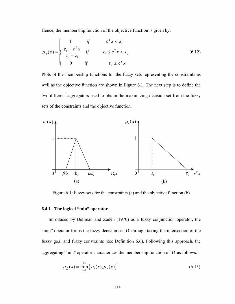
114
Hence, the membership function of the objective function is given by:
1
( )
0
Tl
TTu
z l uu l
Tu
if c x z
z c xx if z c x zz z
if z c x
μ
⎧ <⎪
−⎪= ≤ <⎨ −⎪⎪ ≤⎩
(6.12)
Plots of the membership functions for the fuzzy sets representing the constraints as
well as the objective function are shown in Figure 6.1. The next step is to define the
two different aggregators used to obtain the maximizing decision set from the fuzzy
sets of the constraints and the objective function.
Figure 6.1: Fuzzy sets for the constraints (a) and the objective function (b)
6.4.1 The logical “min” operator
Introduced by Bellman and Zadeh (1970) as a fuzzy conjunction operator, the
“min” operator forms the fuzzy decision set D through taking the intersection of the
fuzzy goal and fuzzy constraints (see Definition 6.6). Following this approach, the
aggregating “min” operator characterizes the membership function of D as follows:
{ }2
1( ) min ( ), ( )
m
i zD ix x xμ μ μ
== (6.13)
ibβ ibαib iD x
( )μi x
1
0 lz uz Tc x
( )μz x
1
0
(a) (b)
115
Since the decision maker is interested in a crisp solution rather than a fuzzy set, the
maximizing optimal decision is obtained via solving the following problem:
{ }2
10 0max ( ) max min ( ), ( )
m
i zD ix xx x xμ μ μ
=≥ ≥= (6.14)
Introducing one new variable [0,1]λ∈ , which essentially corresponds to ( )D xμ in
(6.13), and carrying out some manipulations, the approximate auxiliary formulation
for model (6.8) is given by:
Maximize λ
Subject to Ax b′≤
( ) Tu l uz z c x zλ − + ≤
( 1)i i ib D x bλ β β− + ≥ 21,....,i m= (6.15)
( 1)i i ib D x bλ α α− + ≤ 21,....,i m=
, 0x λ ≥
1λ ≤
Hence, the maximizing crisp solution is obtained through solving model (6.15),
which has one more variable and 2 1m + additional constraints. It should be noted that
although the logical “min” operator has proven to be computationally efficient, it is
not compensatory in the sense that it provides no tradeoff between the degrees of
membership of the fuzzy sets at hand. As explained by Miller et al. (1997), there may
not be any change in the degree of membership of the resulting aggregated fuzzy set
even if the degree of membership in some of the fuzzy sets intersected is increased.
To overcome such limitation, an alternative approach is presented below.
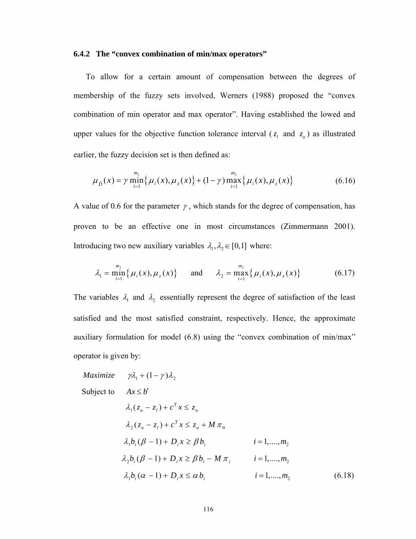
116
6.4.2 The “convex combination of min/max operators”
To allow for a certain amount of compensation between the degrees of
membership of the fuzzy sets involved, Werners (1988) proposed the “convex
combination of min operator and max operator”. Having established the lowed and
upper values for the objective function tolerance interval ( lz and uz ) as illustrated
earlier, the fuzzy decision set is then defined as:
{ } { }2 2
1 1( ) min ( ), ( ) (1 ) max ( ), ( )
m m
i z i zD i ix x x x xμ γ μ μ γ μ μ
= == + − (6.16)
A value of 0.6 for the parameter γ , which stands for the degree of compensation, has
proven to be an effective one in most circumstances (Zimmermann 2001).
Introducing two new auxiliary variables 1 2, [0,1]λ λ ∈ where:
{ }2
1 1min ( ), ( )
m
i zix xλ μ μ
== and { }
2
2 1max ( ), ( )
m
i zix xλ μ μ
== (6.17)
The variables 1λ and 2λ essentially represent the degree of satisfaction of the least
satisfied and the most satisfied constraint, respectively. Hence, the approximate
auxiliary formulation for model (6.8) using the “convex combination of min/max”
operator is given by:
Maximize 1 2(1 )γλ γ λ+ −
Subject to Ax b′≤
1 ( ) Tu l uz z c x zλ − + ≤
2 0( ) Tu l uz z c x z Mλ π− + ≤ +
1 ( 1)i i ib D x bλ β β− + ≥ 21,....,i m=
2 ( 1)i i i ib D x b Mλ β β π− + ≥ − 21,....,i m=
1 ( 1)i i ib D x bλ α α− + ≤ 21,....,i m= (6.18)

117
2 ( 1)i i i ib D x b Mλ α α π− + ≤ + 21,....,i m=
2
20
m
ii
mπ=
≤∑
1 2, , 0x λ λ ≥
{ }0,1iπ ∈
1 2, 1λ λ ≤
Where M is a very large positive number. The constraint 2
20
m
ii
mπ=
≤∑ ensures that at
least one iπ is set to a zero value indicating that the corresponding constraint on 2λ is
satisfied. Notice the increase in model (6.18) dimensionality as compared to that of
models (6.8) and (6.15) above, due to the introduction of auxiliary variables and
constraints.
6.5 The fuzzy production planning model
The fuzzy model presented in this section is similar to the original model initially
introduced in Chapter 3 except that the MPS is now constructed based on confirmed
customers orders which appear in the flexible demand balance constraints. The
mathematical model is presented below.
( ) ( )
( ) ( )
2 2
1 1 1 1 1 1 1 1
21 1 2
1 1 1 1 1
I J T J T Tk k k k k k
t ijt ijt ijt jt jt jt jt t ti j k t j k t t
I T J Tk k k k k kit it it it it it jt jt jt
i k t j t
Z SC S PC X IF I BC B POO
OR G CR Q IR I W SP SP
= = = = = = = =
= = = = =
= + + + +
+ + + + −
∑∑∑∑ ∑∑∑ ∑
∑∑∑ ∑∑
Sibject to k k k
it it itQ M G≤ , ,i t k∀ (6.20)
(6.19)
Min

118
2
1 1 1
1I J
kijt
i j k
Sb= = =
=∑∑∑ t∀ (6.21)
'2
' , 1 '' , 1
' 1 1 ' 1 '
0.4 24kI Ji j tk k k k
ijt ijt i j t ij ijti j k i j
XS Sb S ST Sd
α′ −
′ −′= = = ′
⎛ ⎞⎛ ⎞⎛ ⎞⎜ ⎟= × − + + ×⎜ ⎟⎜ ⎟⎜ ⎟⎜ ⎟⎜ ⎟⎝ ⎠⎝ ⎠⎝ ⎠
∑∑∑ , , ,i j t k∀ (6.22)
2
1 1 1
kI Jijt k
ijt t ti j k ij
XS A O
α= = =
⎛ ⎞+ ≤ +⎜ ⎟⎜ ⎟
⎝ ⎠∑ ∑ ∑ t∀ (6.23)
t otO A≤ t∀ (6.24)
( )k k kijt t ijt ijt ijX b Sb Sd ρ= × + × , , ,i j t k∀ (6.25)
, 11
Jk k k k kit i t it t ijt ijt
jI I Q b Sb Sd−
=
⎡ ⎤= + − × +⎣ ⎦∑ , ,i t k∀ (6.26)
1 1 1 1 1 1 1
, 1 , 1 , ,1
I
j t j t j t j t ijt jt jti
I B I B X W CO− −=
− − + + − ≅∑ ,j t∀ (6.27)
2 2 2 2 2 2, , , 1 , 1
1
I
j t j t j t j t ijt jti
I B I B X W− −=
− = − + −∑ ,j t∀ (6.28)
1 2 2jt jt jtW W CO+ ≅ ,j t∀ (6.29)
0 0 0k k kj j jTI B B= = = ,j k∀ (6.30)
, , , , , , , 0k k k k k k kijt it ijt t jt it jt jtSd Q X O W I I B ≥ , , ,i j t k∀ (6.31)
{ }, 0,1k kit ijtG Sb ∈ , , ,i j t k∀ (6.32)
kijtSd N∈ , , ,i j t k∀ (6.33)
The above mathematical model is fuzzy mixed integer bilinear program
(FMIBLP), where the fuzziness existent in the model arises due to constraints (6.27)
and (6.29) which are treated as flexible constraints and are represented by fuzzy sets
having triangular membership functions. Clearly, conventional mathematical
approaches lack the ability to directly handle such class of models due to the fuzzy
nature of these models. As such, a quick remedy to the existent fuzziness is to adopt
119
the procedure outlined in Section 6.4 with a minor modification that incorporates
bilinear rather than linear programs. The upper and lower tolerance limits on the
objective function value (i.e., uz and lz ) are obtained via fixing the customers orders
at their three possible values, “ * kjtCOβ , k
jtCO , * kjtCOα ” for all , ,j t k and then solving
the corresponding three crisp models (the solution algorithm is outlined in the next
section). Let 1z , 2z and 3z be the obtained values for the objective function of the three
models, then lz min= 1 2 3( , , )z z z and uz max= 1 2 3( , , )z z z , which define the
membership function for the objective function as shown in Equation (6.12).
In most situations and for realistic cost figures, solving the model with the
smallest possible value for the demand, * kjtCOβ , and the highest possible value,
* kjtCOα , yields the values for lz and uz respectively. This is the case since a high
demand value in period t is likely to reduce the major setup cost in period 1t + but it
also entails an increase in most other cost components such as RM purchasing, RM
and FP inventory holding, production and minor setup costs. Having the membership
functions for the objective function and the constraints at hand, the above production
planning fuzzy model is transformed into an equivalent and larger sized crisp model,
depending on the aggregation operator being used as detailed below.
6.6 Auxiliary models description
We present the approximate auxiliary models resulting from the application of the
two different aggregation operators described in Section 6.4. The adoption of these
two particular operators stems from the fact that most other operators, especially
those that are compensatory in nature, produce crisp models that are no longer linear.
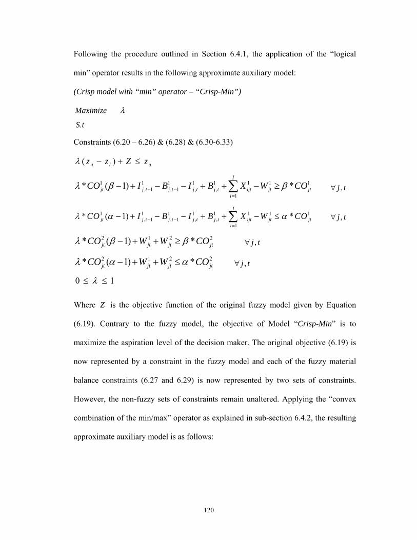
120
Following the procedure outlined in Section 6.4.1, the application of the “logical
min” operator results in the following approximate auxiliary model:
(Crisp model with “min” operator – “Crisp-Min”)
Maximize λ
S.t Constraints (6.20 – 6.26) & (6.28) & (6.30-6.33)
( )u l uz z Z zλ − + ≤
1 1 1 1 1 1 1 1, 1 , 1 , ,
1
* ( 1) *I
jt j t j t j t j t ijt jt jti
CO I B I B X W COλ β β− −=
− + − − + + − ≥∑ ,j t∀
1 1 1 1 1 1 1 1, 1 , 1 , ,
1
* ( 1) *I
jt j t j t j t j t ijt jt jti
CO I B I B X W COλ α α− −=
− + − − + + − ≤∑ ,j t∀
2 1 2 2* ( 1) *jt jt jt jtCO W W COλ β β− + + ≥ ,j t∀
2 1 2 2* ( 1) *jt jt jt jtCO W W COλ α α− + + ≤ ,j t∀
0 1λ≤ ≤
Where Z is the objective function of the original fuzzy model given by Equation
(6.19). Contrary to the fuzzy model, the objective of Model “Crisp-Min” is to
maximize the aspiration level of the decision maker. The original objective (6.19) is
now represented by a constraint in the fuzzy model and each of the fuzzy material
balance constraints (6.27 and 6.29) is now represented by two sets of constraints.
However, the non-fuzzy sets of constraints remain unaltered. Applying the “convex
combination of the min/max” operator as explained in sub-section 6.4.2, the resulting
approximate auxiliary model is as follows:

121
(Crisp model with “convex combination of Min/Max” operator – “Crisp-Comb”) Maximize 1 2(1 )γλ γ λ+ − S.t Constraints (6.20 – 6.26) & (6.28) & (6.30-6.33)
1 ( )u l uz z Z zλ − + ≤
2 1( )u l uz z Z z Mλ π− + ≤ +
1 1 1 1 1 1 1 11 , 1 , 1 , ,
1
* ( 1) *I
jt j t j t j t j t ijt jt jti
CO I B I B X W COλ β β− −=
− + − − + + − ≥∑ ,j t∀
1 1 1 1 1 1 1 12 , 1 , 1 , , 2
1
* ( 1) *I
jt j t j t j t j t ijt jt jti
CO I B I B X W CO Mλ β β π− −=
− + − − + + − ≥ −∑ ,j t∀
1 1 1 1 1 1 1 11 , 1 , 1 , ,
1
* ( 1) *I
jt j t j t j t j t ijt jt jti
CO I B I B X W COλ α α− −=
− + − − + + − ≤∑ ,j t∀
1 1 1 1 1 1 1 12 , 1 , 1 , , 2
1
* ( 1) *I
jt j t j t j t j t ijt jt jti
CO I B I B X W CO Mλ α α π− −=
− + − − + + − ≤ +∑ ,j t∀
2 1 2 21 * ( 1) *jt jt jt jtCO W W COλ β β− + + ≥ ,j t∀
2 1 2 22 3* ( 1) *jt jt jt jtCO W W CO Mλ β β π− + + ≥ − ,j t∀
2 1 2 21 * ( 1) *jt jt jt jtCO W W COλ α α− + + ≤ ,j t∀
2 1 2 22 3* ( 1) *jt jt jt jtCO W W CO Mλ α α π− + + ≤ + ,j t∀
1 2 3 2π π π+ + ≤
{ }1 2 3, , 0,1π π π ∈
1 20 , 1λ λ≤ ≤
It is the objective of model “Crisp-Comb” to achieve a balance between the “max”
operator (i.e., degree of satisfaction of the most satisfied constraint) and the “min”
operator (i.e., degree of satisfaction of the least satisfied constraint). While the

122
original objective function (6.19) is now represented by two constraints, each of the
fuzzy constraints (6.27 and 6.29) is represented by four sets of constraints: two for the
“min” operator and the other two for the “max” operator. Moreover, three binary
variables have been added to the model: one for the objective function and the other
two correspond to each set of the fuzzy constraints.
6.7 Solution Algorithm
The three variants of the original fuzzy model, which are obtained via fixing the
demand at its three respective values (pessimistic, most likely, optimistic), as well as
the auxiliary models resulting from the application of the two different aggregation
operators (i.e., “Crisp-Min” and “Crisp-Comb”) are all mixed integer bilinear
programs (MIBLP). In Chapter 4, we discussed three different “exact” solution
algorithms that generate the optimal solution for this class of models, with varying
computational efficiency. In this section, however, we propose a “non-exact” solution
methodology that is comprised of two phases. In phase 1, the linearization scheme of
Glover (1975) is employed (once more) in order to yield an equivalent linear model.
In phase 2, an exterior penalty function based approach that targets the complicating
constraints is applied to the linearized model resulting from phase 1. The justification
behind the use of an algorithm that is likely to generate “near optimal” production
plans under the dynamic operating conditions is provided later.
Recall that the generic linearization approach of Glover (1975) results in the
following sets of constraints to replace constraint (6.22):
9.6 0.4k k k kijt ijt ijt ij ijtS Sb y ST Sd= × − × + × , , ,i j t k∀ (6.34)

123
k k k k kijt ijt ijt ijt ijtL Sb y U Sb≤ ≤ , , ,i j t k∀ (6.35)
( ) ( )' '
' , 1 ' , 1' '' , 1 ' , 1
' ' ' '' '
1 1k ki j t i j tk k k k k k k
i j t ijt ijt ijt i j t ijt ijti j k i j ki j i j
X XS U Sb y S L Sb
α α′ ′− −
′ ′− −′ ′′ ′
⎛ ⎞ ⎛ ⎞+ − − ≤ ≤ + − −⎜ ⎟ ⎜ ⎟⎜ ⎟ ⎜ ⎟
⎝ ⎠ ⎝ ⎠∑ ∑
, , ,i j t k∀ (6.36)
Although the linearized model resolves the bilinearity issue, such solution might
not be attainable within acceptable time limit especially as the problem size increases.
This is mainly due to the complicating constraint (6.33) which limits the production
to full batches only (i.e., number of batches produced assume only integer values).
The impact of this constraint on the computational complexity was quantified in the
approximate rolling horizon models of Chapter 5. In general, Steel mills would
typically prefer to produce full batches as this implies a more efficient utilization of
the available capacity and better complies with the economies of scale. However, in
reality, production does not always take place in full batches particularly when the
Company is facing low demand or when there is a limited storage space available or a
shortage in the raw material supplies. Moreover, since it is difficult in practice to
obtain a precise estimate for the cost figures, especially when it comes to backlogging
cost for instance, the use of a model that provides valid and efficient proxies for the
total cost function is highly desirable in these situations. The classical approach
within the context of flexible mathematical programming to deal with impreciseness
in cost parameters (e.g. Zimmerman 1976) is to represent the objective function with
a monotonically decreasing linear fuzzy set where the interval of allowance for such
set (i.e., lz and uz ) is decided upon based on a purely subjective judgment obtained
from the decision maker. Our approach, however, provides viable estimates, if not the
exact value, for the case where production takes place in integral batches. More

124
importantly, it also takes into account the flexibility in customers’ orders that the
decision maker is willing to undertake during the planning process which naturally
contributes to the total cost to be incurred. Hence, restricting the production to full
batches achieves only limited added value at the expense of substantial computational
efforts. Wang (1997) points out that, in general, the data are imprecise in a fuzzy
environment, thus, it is meaningless to calculate an exact solution. According to
Hoffman and Padberg (2007), in today’s changing and competitive industrial
environment the difference between using a “quickly derived solution” and using
sophisticated mathematical models to find an “optimal solution” can determine
whether or not a company survives.
It should be noted, however, that relaxing the integrality restriction on the number
of batches produced implies an additional cost that shall be augmented into the
objective function. The augmentation of the deviations from integer batches, we refer
to the sum of such deviations as “integrality gap”, is accounted for through a
penalizing factor that is increased iteratively in an attempt to reduce these deviations
and eventually reach a solution that assumes integer values or within some allowable
gap ε . This procedure falls under the category of exterior penalty function methods
(EPFM) which represent an indirect optimization approach. We provide below a
glimpse of these well-established methods where more details can be usually found in
integer and nonlinear optimization textbooks such as Bazaraa et al. (1993) and Griva
et al. (2009).
In its original context, EPFM augments all the constraints into the objective
function to transform the original problem into an unconstrained optimization

125
problem. A sequential unconstrained minimization technique (SUMT) is then
employed in order to approach the feasible region of the original problem from the
outside, hence the term exterior, until the solution of the unconstrained problem is
made (nearly) equivalent to that of the original one through increasing the value of
the penalty factor in each iteration. This sequential increase in the penalty parameter
avoids the ill-conditioning difficulties associated with the Hessian matrix as the value
of such parameter approaches infinity (more on ill-defining condition can be found in
Sherali et al. (2001), Griva et al. (2009) and Bazaraa et al. (1993). In general, penalty
function methods are usually more convenient than barrier methods for problems with
equality constraints (Griva et al. 2009).
Prior to augmenting the integrality restriction to the objective function, it has to be
first reformulated as an equality constraint. Hence, constraint (6.33) can be
equivalently expressed using either one of the following two forms:
0k kijt ijtSd Sd⎡ ⎤ − =⎢ ⎥ or 0k k
ijt ijtSd Sd⎢ ⎥− =⎣ ⎦
where kijtSd⎡ ⎤⎢ ⎥ and k
ijtSd⎢ ⎥⎣ ⎦ represent the smallest integer greater than or equal to kijtSd
and the largest integer less than or equal to kijtSd , respectively. Although both
equations serve the same purpose mathematically, the first is more appropriate in our
analysis as it shows by how much the production is short of a complete batch. In
reality, this difference has the physical interpretation of “capacity underutilization” as
it shows the amount that could have been produced using the same setup. Hence, the
capacity underutilization cost (CUUC) is given by:

126
( )1 1 1 1
I J K Tk k
l ijt ijti j k t
CUUC Sd Sdμ= = = =
⎡ ⎤= −⎢ ⎥∑∑∑∑ (6.37)
The penalty parameter, lμ , bares the meaning of an underutilization cost per batch
and l is the iteration counter. Deviations from integrality for any RM-FP-SG
combination have the same relative importance and are therefore penalized equally at
a particular iteration. Otherwise, subscripts ,i j and k can be included in the
parameter lμ in order to assign different weights to deviations from integrality for
different combinations. The auxiliary function involving the penalty term is thus
given by pZ Z CUUC= + . Clearly, if the deviations in equation (6.37) add up to
zero, an optimal solution has been found where all the kijtSd variables assume integer
values.
On another note, the setup time calculation is still based on an integral number of
batches since in reality a setup takes place regardless of the batch size produced. As
such, the setup time constraint (6.34) is now reformulated as:
9.6 0.4k k k kijt ijt ijt ij ijtS Sb y ST Sd⎡ ⎤= × − × + × ⎢ ⎥ , , ,i j t k∀ (6.38)
Hence, the three crisp variants of the original fuzzy model, obtained through
fixing the demand at its three respective values, as well as the approximate auxiliary
crisp models obtained after aggregation are now solved using the penalized objective
function pZ instead of Z while dropping the integrality restriction (6.33) out of the
model. Clearly, such changes are also made to the linearized version of these models.
At each iteration, the resulting MILP model is solved directly using AMPL/CPLEX
11.0 solver. The iterative increase in the penalty parameter coupled with a setup time,
127
and accordingly a setup cost, that is calculated based on integral batches, shall force
the model to seek the production of full batches as much as possible. We point out
here that the above application of EPFM to the models at hand is similar in principle
to the idea of Lagrangian relaxation except that in the latter case the penalty terms
(denoted as Lagrange multipliers) are optimized, rather than decided upon
subjectively and increased iteratively, via sub-gradient optimization techniques for
example. The solution algorithm can now be formally stated as follows:
Initialization step:
- Obtain the linearized version of the model, replace Z with pZ and kijtSd with
kijtSd⎡ ⎤⎢ ⎥ in constraint (6.34), drop constraint (6.33) out of the model.
- Define a small tolerance value 0ε ≥ as the deviations related termination scalar,
and 0τ ≥ as the time related termination criterion.
- Choose an initial solution (not necessarily feasible), say 1η , a penalty parameter
1 0μ > and a scalar 1δ > .
- Let the iteration counter 1v = and go to step 1.
Step 1:
- Starting with vη , solve the minimization problem at hand directly using
AMPL/CPLEX 11.0 solver.
- Let 1vη + be the optimal solution and go to step 2.

128
Step 2:
If ( )k kijt ijt
ijktSd Sd ε⎡ ⎤ − ≤⎢ ⎥∑ or if solution time τ= , stop; otherwise, let
1v vμ δμ+ = and 1v v= + and go back to step 1.
The value of the allowable computational time to attain a solution is decided upon by
the decision maker. This time related termination criterion is added to the algorithm
since for very high values of the penalty parameterμ , the capacity underutilization
cost now bares more weight than the rest of the cost components and the model will
continuously seek the minimum possible value for it. As the value of μ approaches
infinity, no savings in computational time is achieved as compared to the original
model which assumes integer values for the variables kijtSd . Hence, the objective is to
find a penalty value that provides for a good compromise between the deviation from
integral batches and the required solution time.
6.8 Computational Experiments
To provide more insights into the performance of the developed mathematical
models as well as that of the above solution methodology, ten problem instances of
different sizes are tested. For each of these ten problems, the two auxiliary models
(i.e., “Crisp-Min” and “Crisp-Comb”) are solved for the same set of input parameters
in order to ensure a fair comparison. While those values for the rest of input
parameters are retained once solving the three variants of the fuzzy model, demand
changes its value corresponding to either one of the three possible values (pessimistic,
most likely, optimistic). As before, the numerical experiments are implemented on a
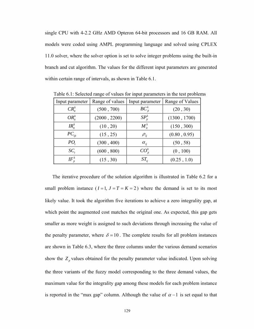
129
single CPU with 4-2.2 GHz AMD Opteron 64-bit processors and 16 GB RAM. All
models were coded using AMPL programming language and solved using CPLEX
11.0 solver, where the solver option is set to solve integer problems using the built-in
branch and cut algorithm. The values for the different input parameters are generated
within certain range of intervals, as shown in Table 6.1.
Table 6.1: Selected range of values for input parameters in the test problems
Input parameter Range of values Input parameter Range of Values kitCR (500 , 700) k
jtBC (20 , 30) kitOR (2000 , 2200) k
jtSP (1300 , 1700) kitIR (10 , 20) k
itM (150 , 300)
ijtPC (15 , 25) ijρ (0.80 , 0.95)
tPO (300 , 400) ijα (50 , 58)
tSC (600 , 800) kjtCO (0 , 100)
kjtIF (15 , 30) ijST (0.25 , 1.0)
The iterative procedure of the solution algorithm is illustrated in Table 6.2 for a
small problem instance ( 1,I = 2J T K= = = ) where the demand is set to its most
likely value. It took the algorithm five iterations to achieve a zero integrality gap, at
which point the augmented cost matches the original one. As expected, this gap gets
smaller as more weight is assigned to such deviations through increasing the value of
the penalty parameter, where 10δ = . The complete results for all problem instances
are shown in Table 6.3, where the three columns under the various demand scenarios
show the pZ values obtained for the penalty parameter value indicated. Upon solving
the three variants of the fuzzy model corresponding to the three demand values, the
maximum value for the integrality gap among these models for each problem instance
is reported in the “max gap” column. Although the value of 1α − is set equal to that

130
of 1 β− indicating a symmetric triangular membership functions for the various
products demands, the obtained values for the augmented objective function are not
symmetric which can be attributed in part to the bilinearity existent in the model.
While the first six problems meet the first stoppage criterion in which the integrality
gap is less than a small tolerance value ( 1ε = ), a running time of 12 hours for the last
four problems is the deciding factor. In all test problems, fixing the demand at its
most pessimistic and optimistic values yield the values for lz and uz , respectively.
Table 6.2: Summary of the results for a small problem instance
Iteration counter
(v)
Penalty (µv)
Integrality Gap
Capacity underutilization
cost (CUUT) Z Zp
1 10 3.3077 33 457,306 457,339
2 100 2.3077 231 457,360 457,591
3 1,000 1.3077 1,308 457,662 458,969
4 10,000 1.3077 13,077 457,662 470,739
5 100,000 0 0 509,187 509,187
Table 6.3: The obtained results for the ten problem instances
Problem instance
Problem size (I×J×T×K)
Pessimistic demand
Most likely demand
Optimistic demand
Penalty (µ)
Max. gap α β
1 (1×2×2×2) 395,534 509,187 594,937 100,000 0 1.2 0.8
2 (1×3×3×2) 792,958 912,498 1,086,102 100,000 0 1.2 0.8
3 (2×3×3×2) 747,795 877,137 1,021,215 100,000 0 1.2 0.8
4 (2×3×4×2) 1,191,695 1,360,073 1,534,557 100,000 0 1.2 0.8
5 (3×4×4×2) 1,370,708 1,546,901 1,711,847 100,000 0.0823 1.2 0.8
6 (4×4×4×2) 1,256,410 1,425,603 1,606,243 10,000 0.9075 1.15 0.85
7 (4×5×4×2) 1,412,311 1,562,135 1,750,538 10,000 1.5659*1.15 0.85
8 (5×5×4×2) 1,440,165 1,602,495 1,791,857 10,000 1.8368*1.15 0.85
9 (5×6×4×2) 1,483,096 1,637,422 1,808,136 10,000 2.6960*1.15 0.85
10 (5×7×5×2) 2,079,562 2,255,339 2,417,524 10,000 4.7902*1.15 0.85* Time related stoppage criterion (Code execution was interrupted after 12 hours of run time)
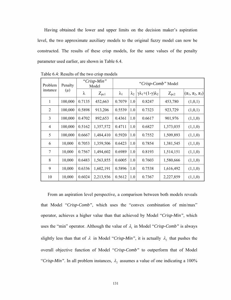
131
Having obtained the lower and upper limits on the decision maker’s aspiration
level, the two approximate auxiliary models to the original fuzzy model can now be
constructed. The results of these crisp models, for the same values of the penalty
parameter used earlier, are shown in Table 6.4.
Table 6.4: Results of the two crisp models
“Crisp-Min” Model “Crisp-Comb” Model Problem
instance Penalty
(µ) λ Zpc1 λ1 λ2 γλ1+(1-γ)λ2 Zpc2 (π1, π2, π3)
1 100,000 0.7135 452,663 0.7079 1.0 0.8247 453,780 (1,0,1)
2 100,000 0.5898 913,206 0.5539 1.0 0.7323 923,729 (1,0,1)
3 100,000 0.4702 892,653 0.4361 1.0 0.6617 901,976 (1,1,0)
4 100,000 0.5162 1,357,572 0.4711 1.0 0.6827 1,373,035 (1,1,0)
5 100,000 0.6667 1,484,410 0.5920 1.0 0.7552 1,509,893 (1,1,0)
6 10,000 0.7053 1,359,506 0.6423 1.0 0.7854 1,381,545 (1,1,0)
7 10,000 0.7567 1,494,602 0.6989 1.0 0.8193 1,514,151 (1,1,0)
8 10,000 0.6483 1,563,855 0.6005 1.0 0.7603 1,580,666 (1,1,0)
9 10,000 0.6336 1,602,191 0.5896 1.0 0.7538 1,616,492 (1,1,0)
10 10,000 0.6024 2,213,936 0.5612 1.0 0.7367 2,227,859 (1,1,0)
From an aspiration level perspective, a comparison between both models reveals
that Model “Crisp-Comb”, which uses the “convex combination of min/max”
operator, achieves a higher value than that achieved by Model “Crisp-Min”, which
uses the “min” operator. Although the value of 1λ in Model “Crisp-Comb” is always
slightly less than that of λ in Model “Crisp-Min”, it is actually 2λ that pushes the
overall objective function of Model “Crisp-Comb” to outperform that of Model
“Crisp-Min”. In all problem instances, 2λ assumes a value of one indicating a 100%

132
satisfaction for the most satisfied constraint. However, this constraint is not always
the same as indicated by the values of the binary variables 1 2 3, ,π π π shown in the
right most column of Table 6.4. However, in terms of the augmented objective
function values ( 1pcZ and 2pcZ ), the total cost of Model “Crisp-Min” is slightly less
than that of Model “Crisp-Comb”.
The advantage of using the fuzzy set theory approach to represent uncertainties in
demand becomes obvious once the resulting auxiliary models are compared with the
crisp counterpart of the original fuzzy model. That is, an initial non-fuzzy formulation
of the problem would treat the fuzzy constraints as strict equalities with the demand
being set to its most likely value. Comparing Models’ “Crisp-Min” and “Crisp-
Comb” total cost with that resulting from the most likely demand given in Table 6.3
shows cost savings in most of the problem instances. In particular, Model “Crisp-
Min” has outperformed the original non-fuzzy model in 8 out of the 10 problem
instances with a slight cost increase for the remaining two problems. Model “Crisp-
Comb”, on the other hand, results in cost savings in 7 out of the 10 problem
instances. A notable increase in the cost savings, as a result of using the fuzzy
approach, is attained as the problem size increases.
6.9 Summary
This chapter has addressed the problem of developing master production schedule
taken into account the uncertainties associated with the end customer demand through
the use of fuzzy set theory (FST). In reality, the decision maker has the ability to
accept or reject orders; a fact that is better accounted for in a mathematical model

133
through flexible demand constraints having triangular membership functions.
Depending on the degree of flexibility that the planner is willing to incorporate, the
limits for the aspiration level are determined and a linear membership function is
formed to represent such level. Due to the difficulty of precisely estimating some of
the cost parameters, “near optimal” solutions were obtained through applying the
classical approach of exterior penalty function methods to a linearized version of the
original model. Such approach results in substantial computational time savings while
still providing valid proxies for the original objective function value.
Besides its major benefit of avoiding the rigid requirements associated with crisp
mathematical programming, the adopted fuzzy approach has proved to result in cost
savings in most situations as compared to the classical deterministic approach. In
general, the performance of the fuzzy models is affected by the choice of the
membership functions and the aggregation operators in the sense that different forms
of functions and operators produce different outcomes. In an attempt to provide a
comparative study between different aggregation operators, we employed the long
established classical “min” operator and the “convex combination of the min/max”
operator in order to obtain the fuzzy decision set.
134
Chapter 7
PART-III: Accounting for Uncertain Demand and Capacity
Using Fuzzy Set Theory Approach
7.1 Introduction
The previous chapter has illustrated the usefulness of the fuzzy set theory (FST)
approach to handle external sources of uncertainties associated with the end customer
demand. In this chapter, we take the previous analysis one step further and
demonstrate the capability of FST to simultaneously handle internal as well as
external sources of uncertainty into the production planning process. In particular,
situations involving imprecise production capacity, such as steel rolling mills, are
tackled through fuzzy mathematical programming techniques. With the latest
advances in technology and the sophisticated manufacturing processes used in several
industries, planning production quantities based on a crisply defined future
production capacity has become unrealistic as many unforeseen events that directly
affect such capacity might occur.
It is the objective of this chapter to illustrate how uncertainty in demand and
imprecise available production capacity and production time per unit can be handled
together through combining the techniques of flexible mathematical programming

135
(FMP) with that of possibilistic programming (PP) within the same mathematical
model. Under the PP approach, we provide a clear distinction between the appropriate
techniques adopted to handle constraints involving fuzzy coefficients only on one
side or on both sides of the constraints. In addition, the effect of the decision maker’s
minimum acceptable possibility level on the final aspiration levels attained is
quantified in the numerical analysis section.
7.2 Possibilistic programming with imprecise technological
coefficients
Possibilistic programming (PP) is concerned with mathematical programs
involving imprecise coefficients that are restricted by possibilistic distributions. In
this section, we consider linear programming problems with imprecise technological
coefficients which can be stated as (Lai and Hwang 1992b):
Min Z c x=
S.t. { }| , 0x X x Ax b x∈ = ≤ ≥ (7.1)
In the model above, c and b are assumed to be defined crisply while A is assumed
imprecise. This study adopts the form of triangualr possibility distribution to
represnet the imprecise coefficients. Generally speaking, a triangular fuzzy number
A is fully characterized using three prominent data values:
(1) The most likely value, mA , that highlights the most belonging memebr to the set of
possible values (possibility degree = 1 once normailized).
(2) The smallest possible value, sA , that least belongs to the set of possible values on
the lower end of the possibility distribution (possibility degree = 0 once normailized).

136
(3) The highest possible value, hA , that least belongs to the set of possible values on
the upper end of the possibility distribution (possibility degree = 0 once normailized).
In the litarature, the “smallest possible” and “highest possible” values are usually
referred to as the “most pessimistic” and the “most optimistic” values, respectively.
Since the “most optimistic” and “most pessimistic” values may switch locations
depending on the physical meaning of the quantity being represnted by a triangular
fuzzy number, we prefer the more generic expressions for these prominent points as
illustrated above.
The problem that arises when attempting to solve model (7.1) is how to conduct
the comparison between the fuzzy consumed resources ( Ax ) and the available crisp
resources (b ). To resolve such fuzzy constraints, we present two approaches that seek
to obtain crisp representative numbers for the fuzzy consumed resources Ax . Tanaka
et al. (1984) suggested using the weighted average of the upper and lower limits and
then substituting this average back into the original model. Following this approach,
the constraint Ax b≤ is now replaced by the auxiliary constraint:
( )1s hwA x w A x b+ − ≤ (7.2)
where 0 1w< < . The alternative approach, proposed by Lai and Hwang (1992b),
incorporates the three prominent values to obtain the following auxiliary constraint
instead:
1 2 3s m hw A x w A x w A x b+ + ≤ (7.3)
where 1 2 3 1w w w+ + = . Although the decision maker would typically assign the
weights to the three possible values, Lai and Hwang (1992b) obtain the most likely

137
solution via the substitution 116
w = , 246
w = and 316
w = . According to them, the
most likely values are often the most important ones and accordingly should have
more weights. The two boundary values, however, provide boundary solutions and
should bare less weight. If the minimal acceptable possibility θ is given, the auxiliary
crisp constraint now becomes:
1 46
s m hA x A x A x bθ θ θ⎡ ⎤+ + ≤⎣ ⎦ (7.4)
The inclusion of the most likely value in the second approach entails that different
solutions will be obtained for different possibilistic distributions, as shown in Figure
7.1 (Lai and Hwang 1992a). Considering the minimal acceptable possibility is θ ,
equation (7.2) will give the same answer while equation (7.3) would give a higher
crisp value for Ax than for A x′ .
Figure 7.1: Ax is greater than A x′ for the accepted possibility level of θ
sA x sA x′
1
θ
(.)π
mA x′ mA x hA x hA x′ /s sA x A x′
A x′ Ax
0
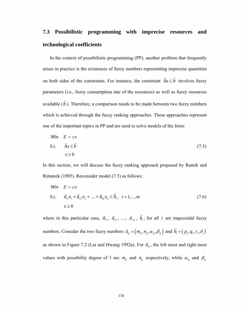
138
7.3 Possibilistic programming with imprecise resources and
technological coefficients
In the context of possibilistic programming (PP), another problem that frequently
arises in practice is the existences of fuzzy numbers representing imprecise quantities
on both sides of the constraints. For instance, the constraint Ax b≤ involves fuzzy
parameters (i.e., fuzzy consumption rate of the resources) as well as fuzzy resources
available (b ). Therefore, a comparison needs to be made between two fuzzy numbers
which is achieved through the fuzzy ranking approaches. These approaches represent
one of the important topics in PP and are used to solve models of the form:
Min Z cx=
S.t. Ax b≤ (7.5)
0x ≥
In this section, we will discuss the fuzzy ranking approach proposed by Ramik and
Rimanek (1985). Reconsider model (7.5) as follows:
Min Z cx=
S.t. 1 1 2 2 ....i i in n ia x a x a x b+ + + ≤ , 1,...,i m= (7.6)
0x ≥
where in this particular case, 1ia , 2ia , …, ina , ib , for all i are trapezoidal fuzzy
numbers. Consider the two fuzzy numbers ( ), , ,ij ij ij ij ija m n α β= and ( ), , ,i i i i ib p q τ δ=
as shown in Figure 7.2 (Lai and Hwang 1992a). For ija , the left most and right most
values with possibility degree of 1 are ijm and ijn respectively, while ijα and ijβ

139
represent the respective left and right spreads. A similar argument applies to the fuzzy
number ib .
Figure 7.2: The representation of fuzzy inequality of two fuzzy numbers
Using the set-inclusion concept, Ramik and Rimanek (1985) asserted that:
ij ia b≤ if and only if ij im p≤ , ij in q≤ , ij ij i im pα τ− ≤ − and ij ij i in qβ δ+ ≤ + (7.7)
Excluding the case of 1 2 ... 0nx x x= = = = , we obtain the following equivalent crisp
linear programming problem:
Min Z cx= S.t.
ij j ij
m x p≤∑ i∀
ij j ij
n x q≤∑ i∀
( )ij ij j i ij
m x pα τ− ≤ −∑ i∀ (7.8)
(.)π 1
ij ijm α− ijm ipi ip τ−
i ja ib
0 ijn ij ijn β+iq i iq δ+

140
( )ij ij j i ij
n x qβ δ+ ≤ +∑ i∀
0x ≥
The solution to model (7.8) is also considered to be the solution to model (7.6). We
also point out that other fuzzy ranking approaches exist such as that of Tanaka et al.
(1984) for triangular fuzzy numbers.
7.4 The fuzzy production planning model
In the context of fuzzy mathematical programming, two very different issues can
be addressed: fuzzy or flexible constraints for fuzziness, and fuzzy coefficients for
lack of knowledge or epistemic uncertainty (Peidro et al. 2009). As illustrated in the
previous chapter, several authors have addressed problems in which either type of
fuzziness arises. In fact, it was not till recently when only few authors have
simultaneously considered problems involving both types of fuzziness (e.g., Mula et
al. 2007 and Peidro et al. 2009).
Typically, steel mills, as well as other process industries, operate in an
environment in which internal and external sources of uncertainty affect its mode of
operation and consequently the production planning related decisions. Such
uncertainties are associated with the available production capacity, which in most
practical situations is hard to specify precisely, and the anticipated customers’
demand, which is frequently prone to errors due to changing customers’ preferences
(as established earlier). The fuzzy mixed integer bilinear programming (FMIBLP)
model presented in this section jointly contemplates the possible lack of knowledge
associated with the production capacity and existing fuzziness in the anticipated
141
demand. Hence, the model involves flexible demand constraints as well as hard
constraints comprising fuzzy quantities on either one side or both sides of the
constraints. In fact, the presented fuzzy model deviates from those in the literature in
combining the approaches of flexible mathematical programming (FMP) and
possibilistic programming (PP) where also the weighted average method (Lai and
Hwang 1992b) and the fuzzy ranking approach (Ramik and Rimanek 1985) are
concurrently employed in order to handle fuzzy quantities within the mathematical
model.
In reality, it is difficult to establish a precise value for the production capacity,
which is mainly comprised of available workforce level and machine uptime. There
are a lot of unforeseen events that contribute to unstable production capacity
including machine breakdowns, longer or shorter than expected repair time and/or
setup time, variable scrap rate resulting from faulty production as well as worker
injuries and/or absenteeism. Hence, the available production time is better represented
by a fuzzy number having a triangular possibility distribution where the optimistic
values of this distribution denote the possibility of working overtime hours.
Moreover, the nature of the bar rolling process, the uniformity of raw material
supplied and the quality of the production line setup might occasionally cause a steel
bar to drift out of its intended path or get stuck on its way through the different rolling
stands causing a complete stoppage to the whole production line in either case. Thus,
it seems more practical to also assume the production rate (or equivalently, the
production time per ton) to be rather a fuzzy number having a triangular possibility
distribution.

142
From a demand perspective, the “rush orders” phenomenon that the steel mill
suffers from is also taken into account during the planning process through flexible
demand constraints. The fuzzy mathematical model presented here jointly considers
both types of uncertainties. As done in Chapter 6, the flexible demand constraints are
also represented by fuzzy sets having triangular membership functions. In addition,
we assume that the available capacity and the production time per ton are fuzzy
numbers having triangular possibility distribution. Such distribution allows for both
positive and negative deviations from a “most likely” value which better reflects on
reality. The fuzzy model is formally stated as follows:
( ) ( )
( ) ( )
2 2
1 1 1 1 1 1 1
21 1 2
1 1 1 1 1
I J T J Tk k k k k k
t ijt ijt ijt jt jt jt jti j k t j k t
I T J Tk k k k k kit it it it it it jt jt jt
i k t j t
Z SC S PC X IF I BC B
OR G CR Q IR I W SP SP
= = = = = = =
= = = = =
= + + +
+ + + + −
∑∑∑∑ ∑∑∑
∑∑∑ ∑∑
S.t
k k k
it it itQ M G≤ , ,i t k∀ (7.10)
2
1 1 11
I Jkijt
i j kSb
= = =
=∑∑∑ t∀ (7.11)
( )2
' '' ' ' , 1 ' , 1
' 1 1 ' 1
0.4 24I J
k k k k kijt ijt i j i j t i j t ij ijt
i j k
S Sb X S ST Sdτ ′ ′− −′= = =
⎛ ⎞⎛ ⎞= × − + + ×⎜ ⎟⎜ ⎟⎜ ⎟⎝ ⎠⎝ ⎠
∑∑∑ , , ,i j t k∀ (7.12)
( )2
1 1 1
I Jk k
ij ijt ijt ti j k
X S Aτ= = =
+ ≤∑ ∑ ∑ t∀ (7.13)
( )k k kijt t ijt ijt ijX b Sb Sd ρ= × + × , , ,i j t k∀ (7.14)
, 11
Jk k k k kit i t it t ijt ijt
jI I Q b Sb Sd−
=
⎡ ⎤= + − × +⎣ ⎦∑ , ,i t k∀ (7.15)
(7.9)
Min

143
1 1 1 1 1 1 1
, 1 , 1 , ,1
I
j t j t j t j t ijt jt jti
I B I B X W CO− −=
− − + + − ≅∑ ,j t∀ (7.16)
2 2 2 2 2 2, , , 1 , 1
1
I
j t j t j t j t ijt jti
I B I B X W− −=
− = − + −∑ ,j t∀ (7.17)
1 2 2jt jt jtW W CO+ ≅ ,j t∀ (7.18)
0 0 0k k kj j jTI B B= = = ,j k∀ (7.19)
, , , , , , 0k k k k k k kijt it ijt jt it jt jtSd Q X W I I B ≥ , , ,i j t k∀ (7.20)
{ }, 0,1k kit ijtG Sb ∈ , , ,i j t k∀ (7.21)
kijtSd N∈ , , ,i j t k∀ (7.22)
Recall that the notion “≅ ” in constraints (7.16) and (7.18) represents the fuzzified
version of “=” and reads “essentially equal to”. On the other hand, the notions “ ijτ ”
and “ tA ” indicate traingular fuzzy numbers characterizing the imprecise production
time per ton and total available production time.
The fuzzy model at hand includes constraints (7.12), which have only imprecise
technological coefficients (i.e., a fuzzy production time per ton) resulting in a fuzzy
quantity only on one side of the constraint, and constraints (7.13) which involve both
imprecise technological coefficients as well as imprecise availability of resources
inducing a comparison between two fuzzy quantities existing on both sides of the
constraint. As illustrated earlier, the first case can be handled using the weighted
average method (WAM), originally proposed by Lai and Hwang (1992b) and
successfully applied afterwards to several problems including aggregate production
planning (e.g., Liang 2007) and supply chain management (Liang 2008). Following
this method, the fuzzy number ijτ is defuzzified and converted to an equivalent crisp

144
value given the decision’s maker minimum acceptable possibility level, and a
subjectively chosen set of weights 1 2 3, ,w w w . Clearly, the resulting crisp value
depends on the initial possibility distribution for fuzzy number, the minimum
acceptable possibility level and the weights assigned, as can be seen in Figure 7.3. In
general, based on the similarity of triangles, the three prominent values corresponding
to the possibility level θ are obtained as follows:
( ),s s m sij ij ij ijθτ τ θ τ τ= + − , ,i j θ∀ (7.23)
,m mij ijθτ τ= , ,i j θ∀ (7.24)
( )( ), 1h m h mij ij ij ijθτ τ θ τ τ= + − − , ,i j θ∀ (7.25)
Notice that the value ,mij θτ is always equal to the initial most likely value m
ijτ and thus
remains unchanged regardless of chosen acceptable possibility level θ .
Figure 7.3: Triangular possibility distribution for the production time per ton ijτ
1
0
( )ijπ τ
θ
ijτ hijτ
mijτ ,
hij θτs
ijτ ,sij θτ

145
Having these three values at hand, the auxiliary crisp equivalence of equation (7.12)
is obtained as:
2' '
' ', ' ', ' ', ' , 1 ' , 1' 1 1 ' 1
1 4 10.4 246 6 6
I Jk k s m h k kijt ijt i j i j i j i j t i j t
i j k
kij ijt
S Sb X S
ST Sd
θ θ θτ τ τ ′ ′− −′= = =
⎛ ⎞⎛ ⎞⎛ ⎞⎛ ⎞= × − + + +⎜ ⎟⎜ ⎟⎜ ⎟⎜ ⎟⎜ ⎟⎝ ⎠⎝ ⎠⎝ ⎠⎝ ⎠+ ×
∑∑∑ (7.26)
In this study, we apply the concept of the most likely values proposed in the original
paper (Lai and Hwang 1992b), where 1 3 1/ 6w w= = and 2 4 / 6w = .
The second scenario, which involves fuzzy quantities on both sides of constraint
(7.13) calls for the employment of fuzzy ranking techniques (e.g. Ramik and
Rimanek 1985). Following this approach, constraint set (7.13) is replaced by the
following three sets of constraints:
( )2
, ,1 1 1
I Js k k sij ijt ijt t
i j kX S Aθ θτ
= = =
+ ≤∑ ∑ ∑ t∀ (7.27)
( )2
, ,1 1 1
I Jm k k mij ijt ijt t
i j kX S Aθ θτ
= = =
+ ≤∑ ∑ ∑ t∀ (7.28)
( )2
, ,1 1 1
I Jh k k hij ijt ijt t
i j kX S Aθ θτ
= = =
+ ≤∑ ∑ ∑ t∀ (7.29)
As the resulting auxiliary model still involves flexible constraints, this model is
solved under the three possible demand values to establish the upper and lower limits
for the linear fuzzy set representing the objective function as presented in Chapter 6.
Also, the models are solved in a similar fashion where the exterior penalty function
method (EPFM) is employed coupled with sequential minimization techniques (SMT)
to minimize the deviations from integral batches. The classical “Min” operator and
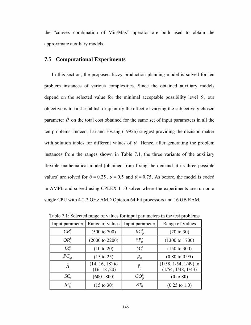
146
the “convex combination of Min/Max” operator are both used to obtain the
approximate auxiliary models.
7.5 Computational Experiments
In this section, the proposed fuzzy production planning model is solved for ten
problem instances of various complexities. Since the obtained auxiliary models
depend on the selected value for the minimal acceptable possibility level θ , our
objective is to first establish or quantify the effect of varying the subjectively chosen
parameter θ on the total cost obtained for the same set of input parameters in all the
ten problems. Indeed, Lai and Hwang (1992b) suggest providing the decision maker
with solution tables for different values of θ . Hence, after generating the problem
instances from the ranges shown in Table 7.1, the three variants of the auxiliary
flexible mathematical model (obtained from fixing the demand at its three possible
values) are solved for 0.25θ = , 0.5θ = and 0.75θ = . As before, the model is coded
in AMPL and solved using CPLEX 11.0 solver where the experiments are run on a
single CPU with 4-2.2 GHz AMD Opteron 64-bit processors and 16 GB RAM.
Table 7.1: Selected range of values for input parameters in the test problems
Input parameter Range of values Input parameter Range of Values kitCR (500 to 700) k
jtBC (20 to 30) kitOR (2000 to 2200) k
jtSP (1300 to 1700) kitIR (10 to 20) k
itM (150 to 300)
ijtPC (15 to 25) ijρ (0.80 to 0.95)
tA (14, 16, 18) to (16, 18 ,20) ijτ (1/58, 1/54, 1/49) to
(1/54, 1/48, 1/43) tSC (600 , 800) k
jtCO (0 to 80) kjtIF (15 to 30) ijST (0.25 to 1.0)
147
The results for the three values for the acceptable possibility level are shown in
Tables 7.2-7.4 below. To help visualize the obtained results, Figures 7.4-7.6 illustrate
the change in the value of the total cost for each of the problems under the three
demand scenarios. As can be seen, there is no significant difference in the cost
obtained as a result of changing the acceptable possibility level. This minor difference
is seen in the figures showing a “seemingly like” one curve which is actually three
curves that plot “more or less” on top of each other. More importantly, there is no
consistent pattern to the behavior of the cost figures due to changing θ values. For
instance, in problem 9, the minimum cost figures for the pessimistic, most likely and
optimistic demand are obtained when 0.5θ = , 0.25θ = and 0.75θ = , respectively.
In problem 10, setting 0.25θ = results in the highest cost under all demand scenarios
although this last consistency seems to be just a coincidence as suggested by the
results obtained for the rest of the problems. This analysis suggests that changing the
value of θ does not significantly affect the solutions obtained. Hence, we carry out
the remaining tests on the resulting equivalent crisp models (after using the
aggregation operators) for only one θ value, 0.5θ = .
Since the linear fuzzy set characterizing the decision maker’s aspiration level is
now established, the next step is to aggregate this set with the feasible solutions set
defined by the constraints in order to obtain the fuzzy decision set using the
previously established “Min” operator, and “Convex Combination of Min/Max”
operator. We denote the first crisp model as “Crisp-Min2” and the second crisp model
“Crisp-Comb2” to distinguish them from those obtained in the previous chapter. The
results for the ten problem instances for both models are shown in Table 7.5.

148
Table 7.2: The obtained results for the ten problem instances for 0.25θ =
Problem instance
Problem size (I×J×T×K)
pessimistic demand
Most likely demand
Optimistic demand
Penalty (µ) Max. gap α β
1 (1×2×2×2) 380,383 489,386 577,717 100,000 0 1.2 0.8
2 (1×3×3×2) 769,570 853,446 1,013,994 100,000 0 1.15 0.85
3 (2×3×3×2) 738,739 841,402 965,628 100,000 0 1.15 0.85
4 (2×3×4×2) 1,053,541 1,184,086 1,306,895 100,000 0.0081 1.15 0.85
5 (3×4×4×2) 1,184,422 1,268,363 1,356,954 100,000 0.3024 1.1 0.9
6 (4×4×4×2) 1,125,123 1,239,076 1,334,282 10,000 0.7962 1.1 0.9
7 (4×5×4×2) 1,290,874 1,402,208 1,500,961 10,000 1.9028* 1.1 0.9
8 (5×5×4×2) 1,326,954 1,431,513 1,550,492 10,000 2.3878* 1.1 0.9
9 (5×6×4×2) 1,461,830 1,588,559 1,708,474 10,000 2.6863* 1.1 0.9
10 (5×7×5×2) 2,017,305 2,115,941 2,237,036 10,000 4.3577* 1.1 0.9
* Time related stoppage criterion (Code execution was interrupted after 12 hours of run time) Table 7.3: The obtained results for the ten problem instances for 0.5θ =
Problem instance
Problem size (I×J×T×K)
pessimistic demand
Most likely demand
Optimistic demand
Penalty (µ) Max. gap α β
1 (1×2×2×2) 380,383 489,386 572,107 100,000 0 1.2 0.8
2 (1×3×3×2) 769,570 846,952 1,013,920 100,000 0 1.15 0.85
3 (2×3×3×2) 738,225 840,976 965,306 100,000 0 1.15 0.85
4 (2×3×4×2) 1,053,541 1,184,655 1,305,361 100,000 0 1.15 0.85
5 (3×4×4×2) 1,182,391 1,268,363 1,356,954 100,000 0.2280 1.1 0.9
6 (4×4×4×2) 1,125,181 1,239,003 1,334,557 10,000 0.7435 1.1 0.9
7 (4×5×4×2) 1,295,916 1,411,518 1,501,294 10,000 1.9382* 1.1 0.9
8 (5×5×4×2) 1,317,144 1,432,356 1,557,540 10,000 2.5520* 1.1 0.9
9 (5×6×4×2) 1,460,381 1,590,823 1,707,538 10,000 2.8467* 1.1 0.9
10 (5×7×5×2) 2,009,941 2,111,660 2,229,487 10,000 4.0779* 1.1 0.9
* Time related stoppage criterion (Code execution was interrupted after 12 hours of run time)

149
Table 7.4: The obtained results for the ten problem instances for 0.75θ =
Problem instance
Problem size (I×J×T×K)
pessimistic demand
Most likely demand
Optimistic demand
Penalty (µ) Max. gap α β
1 (1×2×2×2) 380,383 489,386 572,107 100,000 0 1.2 0.8
2 (1×3×3×2) 769,570 846,731 1,013,994 100,000 0 1.15 0.85
3 (2×3×3×2) 738,872 841,655 965,717 100,000 0 1.15 0.85
4 (2×3×4×2) 1,053,541 1,183,541 1,303,976 100,000 0 1.15 0.85
5 (3×4×4×2) 1,180,617 1,268,547 1,356,954 100,000 0.1907 1.1 0.9
6 (4×4×4×2) 1,125,928 1,239,421 1,334,285 10,000 0.6013 1.1 0.9
7 (4×5×4×2) 1,292,386 1,409,180 1,509,396 10,000 1.8559* 1.1 0.9
8 (5×5×4×2) 1,317,728 1,430,793 1,555,141 10,000 2.5121* 1.1 0.9
9 (5×6×4×2) 1,468,541 1,595,085 1,698,357 10,000 2.7642* 1.1 0.9
10 (5×7×5×2) 2,010,782 2,106,754 2,221,203 10,000 4.6310* 1.1 0.9
* Time related stoppage criterion (Code execution was interrupted after 12 hours of run time)
0
500
1000
1500
2000
2500
1 2 3 4 5 6 7 8 9 10Problem instance
Tota
l cos
t (Th
ousa
nds)
Theta = 0.25 Theta = 0.50 Theta 0.75
Figure 7.4: Total cost for various θ values under pessimistic demand scenario

150
0
500
1,000
1,500
2,000
2,500
1 2 3 4 5 6 7 8 9 10Problem instance
Tota
l cos
t (Th
ousa
nds)
Theta = 0.25 Theta = 0.50 Theta = 0.75
Figure 7.5: Total cost for various θ values under the most likely demand scenario
0
500
1,000
1,500
2,000
2,500
1 2 3 4 5 6 7 8 9 10Problem instance
Tota
l cos
t (Th
ousa
nds)
Theta = 0.25 Theta = 0.50 Theta = 0.75
Figure 7.6: Total cost for various θ values under optimistic demand scenario
Comparing the values for the aspiration level obtained using both operators, we
notice that Model “Crisp-Min2” yields a lower value than that of Model “Crisp-
Comb2”. The resulting 2λ value, which expresses the degree of satisfaction of the

151
most satisfied constraints, is responsible for increasing the aspiration level once the
combination of 1λ and 2λ is calculated. However, it should be noted that 2λ achieves
unity in 9 out of the 10 test problems indicating that, in the remaining problem, 100%
satisfaction for the most satisfied constraint could not be achieved. Note that this
constraint is not always the same as indicated by the values of the binary variables
1 2 3, ,π π π shown in the right most column of Table 7.5. However, in terms of the
augmented objective function values ( 1pcZ and 2pcZ ), the total cost of Model “Crisp-
Min2” is always slightly less than that of Model “Crisp-Comb2”.
Table 7.5: Results of the two crisp models
“Crisp-Min2” Model “Crisp-Comb2” Model Problem
instance Penalty
(µ) λ Zpc1 λ1 λ2 γλ1+(1-γ)λ2 Zpc2 (π1, π2, π3)
1 100,000 0.6138 454,426 0.6098 1 0.7659 455,194 (1,0,1)
2 100,000 0.5399 881,995 0.5354 1 0.7213 883,095 (1,0,1)
3 100,000 0.5501 840,389 0.5391 1 0.7235 842,886 (1,1,0)
4 100,000 0.6369 1,144,976 0.6343 1 0.7806 1,145,632 (1,1,0)
5 100,000 0.6067 1,251,047 0.5785 1 0.7471 1,255,969 (1,0,1)
6 10,000 0.6239 1,203,927 0.6046 1 0.7628 1,207,968 (1,1,0)
7 10,000 0.6803 1,361,575 0.6727 0.9747 0.7935 1,363,136 (1,1,0)
8 10,000 0.7441 1,378,661 0.7187 1 0.8312 1,384,767 (1,1,0)
9 10,000 0.7572 1,520,390 0.7254 1 0.8352 1,528,250 (1,1,0)
10 10,000 0.7680 2,060,876 0.7403 1 0.8441 2,066,957 (1,1,0)
At this juncture, a comparison between the performances of the resulting auxiliary
models using both operators with the crisp counterpart of the original fuzzy model is
due. As defined in the previous chapter, the crisp counterpart refers to initial

152
deterministic formulation of the production planning problem with rigid demand
constraint where the value of the demand is set at the most likely value. Upon
comparing Models’ “Crisp-Min2” and “Crisp-Comb2” total cost with that resulting
from the most likely demand given in Table 7.3 shows a cost savings in most of the
problem instances. Except for the second problem instance, Model “Crisp-Min2” has
outperformed the original non-fuzzy model for all other test problems. On the other
hand, Model “Crisp-Comb2” results in cost savings in 8 out of the 10 problem
instances. This illustrates the economical benefits obtained from adopting the FST to
explicitly account for uncertainties in the context of mathematical models.
7.6 Summary
This chapter has simultaneously addressed both external uncertainties associated
with customers’ demand as well as internal uncertainties characterizing the
availability of the manufacturing process. A fuzzy mathematical model that jointly
accounts for both uncertainties is presented in which the techniques of flexible
mathematical programming (FMP) and possibilistic programming (PP) were adopted.
To handle fuzzy coefficients existent in the model, average weighted method with the
most likely solutions and fuzzy ranking approach were utilized. The results obtained
illustrate the benefits obtained from utilizing FST to model uncertainties as compared
to the deterministic approach. The combination of FMP and PP principles to treat
production planning related problems has not received much attention from
researchers and shall thus be a valuable addition to the available literature. This
allows for handling fuzzy quantities of various natures within the same mathematical
model.

153
Chapter 8
Conclusions and Future Research Directions
8.1 Summary and Conclusions
The problem of developing production plans that efficiently utilize the available
resources in process industries, such as steel rolling industry, is of particular interest
to researchers as well as industrial practitioners. Steel manufacturers nowadays face a
stiff competition which brings out the need for consistent efforts towards reducing
costs and improving the customer service level. In particular, production and
inventory related decisions in steel rolling mills, which are characterized by being
both capital and energy intensive, bare a great importance as they have a direct
impact on the financial health of the organization. In this research, the master
production scheduling (MPS) problem in steel rolling mills under static and dynamic
operating conditions has been investigated. As this industry has some distinguishing
characteristics associated mainly with the manufacturing process, an implementable
production schedule has been developed where these features were taken into
account. At first, the MPS was developed under static demand conditions where the
effect of several interrelated factors on the planning decisions was evaluated.
Mathematical programming techniques have been employed in order to determine the

154
optimized production schedules and raw material purchasing quantities while
satisfying the end customer demand.
Since uncertainty is an inherent part of the production environment in which steel
mills operate, two different approaches were adopted to incorporate the uncertainty in
demand into the planning decisions. The first approach to consider demand
uncertainty involved establishing approximate models that are implemented on a
rolling horizon basis where the problem parameters are updated at the beginning of
each period. These approximate models generate only exact schedules and comprise a
tractable number of binary and/or integer variables resulting in substantial savings in
the computational time needed to solve them. The second approach to address
demand uncertainty involved the use of FST in order to express the demand
constraints as flexible constraints in the mathematical model. The utilization of this
approach has resulted in economical benefits as compared to the use of the
deterministic models.
Towards developing a production schedule that considers uncertainties in demand
as well as production capacity, the approaches of flexible mathematical programming
(FMP) and possibilistic programming (PP) have been utilized. The combined use of
these approaches allows uncertainties of different nature to be incorporated into the
same mathematical model. To handle fuzzy quantities involved in the model, we
utilized both the weighted average method and the fuzzy ranking approach.
Throughout this thesis, the (near) optimal solutions to the developed mathematical
models were obtained via various solution algorithms that have different
computational capabilities.

155
8.2 Thesis contributions
The research presented in this thesis has been classified in three parts where each
part tackles a certain aspect of the production planning problem. The first part, which
treats the problem under static demand conditions, has made the following
contributions:
• Literature classification: The production planning problem at hand represents
an instance of the well known dynamic lot-sizing problem (DLSP). Hence, before
attempting to tackle the problem, the related literature concerning the general
DLSP has been classified based on their distinguishing characteristics. In
particular, the contributions made by researchers to the capacitated multi-item
DLSP from a modeling and solution algorithms perspectives have been
highlighted. We also pointed out the equivalence between the MPS problem, as
coined in the production planning literature, and a special class of the DLS
problem, as coined in the inventory management literature.
• Mathematical modeling: The optimized master production schedule is obtained
through the development of a mixed integer bilinear program (MIBLP) that
addresses the problem under static demand conditions. The novelty to this model
is that it jointly accounts for the distinguishing features and technological
constraints associated with the manufacturing process of the bar rolling industry
including complex setup time structure, raw-material finished-product dependent
scrap and production rates, batch manufacturing, overtime, backlogging and
product substitution. The objective of the model is to provide insights into the
combined effect of these interrelated factors. Since this deterministic model

156
establishes the production and inventory related decisions based solely on
customer demand, it is most useful in periods where the company faces low
demand volatility.
• Solution Algorithms: The main contribution in this perspective is a modified-
branch-and-bound (B&B) algorithm that exploits the special structure of the
mathematical model in order to minimize the number of branches to be explored.
Instead of relaxing the binary restriction and obtaining the bound through
continuous relaxations, our algorithm makes proper substitutions of the binary
variables which resolves the existent bilinearity in the model and allows for the
attainment of the bound at each node. An alternative algorithm is the hybrid
linearization-Benders decomposition (BD) approach where the bilinear model is
linearized first and then the resulting MILP is solved using BD. Although
numerical experiments have illustrated that it is more efficient to directly solve
the linearized model using MIP solver such as CPLEX 11.0, the hybrid algorithm
provides an alternative solution methodology to models involving complicating
constraints. The typical approaches to handle these models in the literature are
Dantzig-Wolfe decomposition and Lagrange decomposition. The modified B&B
algorithm have shown better performance capabilities than the linearization
approach for larger problem sizes with a savings in computational time of up to
48%.
In the second part of this research, demand volatility, which takes the form of
“rush orders” due to changing customers’ preferences and heightened expectations of
shortened delivery lead time, is addressed. Two different approaches are employed in

157
order to account for demand uncertainties in the planning decisions which results in
the following contributions:
• Viable rolling horizon approximations: Developing the production schedule on
a rolling horizon basis, where the schedule is updated periodically as new
information becomes available, requires rerunning the exact model at the
beginning of each time period, and hence consumes a great deal of computational
time. As a remedy to this issue, we proposed several viable approximations that
generate exact schedules and relax the complicating constraints only during the
unimplemented periods of the planning horizon. These complicating constraints,
such as integrality restriction on the number of batches produced, prevent the
attainment of quick solutions, hence the approximations allow for quantifying the
effect of the complicating constraints on the computational time needed and on
the total cost obtained. Computational experiments have shown that the
developed approximate models provide valid proxies to the exact model and
result in substantial savings in computational time.
• Flexible mathematical model: Most previous applications of the flexible
mathematical programming (FMP) approach have assumed that the fuzzy set
representing the objective function is known a priori and is represented by a
linear function and the fuzzy set representing the flexible constraint is also linear.
Our analysis departs from these assumptions and deals with non-symmetric
models in which the fuzzy set representing the flexible constraints is represented
by a triangular membership function. As such, instead of establishing the interval
of allowance on the decision maker’s aspiration level (i.e., objective function)

158
based solely on hunches and pure subjective judgment, the amount of flexibility
determined by the fuzzy set of the flexible constraints is used to estimate this
interval. Since such an estimate need not be accurate, a non-exact solution
algorithm based on the exterior penalty function method (EPFM) was
implemented.
The last part of this research is directed towards simultaneously treating the existing
uncertainties in customer demand and available production capacity, resulting in the
following contribution:
• Integration of FMP and PP: In practice, accounting for uncertainties through
the use of fuzzy set theory (FST) into mathematical models might take several
forms depending on the nature of the existent fuzziness in the problem at hand.
Not only we have combined the approaches of FMP and PP into the same
mathematical model, but we also presented a situation that calls for the joint
implementation of the weighted average method and fuzzy ranking approaches in
order to handle fuzzy coefficients appearing on one side or both sides of some
constraints. This contribution opens the door to promising research avenues since
it allows for handling situations involving various sources of uncertainties. Using
these techniques, all uncertainties can now be incorporated into one fuzzy model
and then defuzzified into an equivalent auxiliary crisp model whose solution can
be found using classical optimization tools.
159
8.3 Recommendations for future research
Modeling and optimization of process industries in general has been and
continues to be one of the active research topics requiring further investigation. The
work that has been conducted along this line of research besides the work presented
in this thesis suggest the following future research directions:
• Developing mathematical models that jointly optimize production and
transportation related decisions. In the steel industry for instance, most of the raw
material is bulky which greatly limits the choices for the appropriate
transportation modes. This in turn might have an effect on the availability of raw
materials in the timings and amounts needed.
• Developing multi-objective production-inventory models where, in addition to
cost minimization, other performance measures such as machine utilization and
scrap percentage are also optimized. This allows for the attainment of a
compromise solution that satisfies all of the performance measures to the best
possible extent.
• Implementing heuristic search algorithms to solve mixed integer bilinear
programs (MIBLP) similar to the ones presented in this research. These meta-
heuristics, such as Genetic algorithms, simulated annealing, and tabu search,
have proven successful in obtaining “good quality” solutions to various
combinatorial optimization problems within reasonable amount of computational
time. Hence, the implementation of these heuristics search methods is an area to
be tested furthermore.

160
• Typically, the existing approaches adopted to handle fuzzy models involve first
“defuzzifying” the model and then solving the resulting auxiliary crisp model
without directly attempting to handle the fuzzy model in a more efficient way. As
noted by Lai and Hwang (1992a), research on developing fuzzy algorithms and
coding existing fuzzy approaches in computer packages is urgently needed.
• In practice, firms might face randomness in addition to imprecision/fuzziness
where both phenomena need to be accounted for in the planning process. In the
literature, very little research has been done in the area of probabilistic fuzzy
models and their solution methodologies. This represents an interesting area
which requires further investigation.
• The presented analysis can also be extended to account for the more general
situation where the rolling mill has more than a single production line and
production rates and throughput differ from one production line to the other. In
this scenario, a scheduling problem arises where the assignment of jobs to
machines (i.e., production lines) is determined such that a performance measure,
such as total flow time or makespan, is minimized.

161
Bibliography
Absi, N., Kedad-Sidhoum, S., 2008. The multi-item capacitated lot sizing problem
with setup times and shortage costs. European Journal of Operational Research
185, 1351-1374.
Adams, W.P., Forrester, R.J., 2007. Linear forms of nonlinear expressions: New
insights on old ideas. Operations Research Letters 35, 510–518.
Adams, W.P., Forrester, R.J., Glover, F.W., 2004. Comparisons and enhancement
strategies for linearizing mixed 0-1 quadratic programs. Discrete Optimization 1,
99-120.
Adams, W.P., Sherali, H.D., 1986. A tight linearization and an algorithm for zero-one
quadratic programming problems. Management Science 32, 1274-1290.
Adams, W.P., Sherali, H.D., 1990. Linearization strategies for a class of zero-one
mixed integer programming problems. Operations Research 38 (2), 217–226.
Adams, W.P., Sherali, H.D., 1993. Mixed-integer bilinear programming problems.
Mathematical Programming 59, 279-305.
Aggarwal, A., Park, J.K., 1993. Improved algorithms for economic lot-size problem.
Operations Research 41 (3), 549-571.
Akinc, U., Khumawala, B.M., 1977. An Efficient Branch and Bound Algorithm for
the Capacitated Warehouse Location Problem. Management Science 23 (6), 585-
594.

162
Aksen, D., Altmkemer, K., Chand, S., 2003. The single item lot sizing problem with
immediate lost sales. European Journal of Operational Research 147, 558-566.
Alguacil, N., Conejo, J., 2000. Multi-period optimal power flow using Benders
decomposition. IEEE Transactions on Power Systems 15 (1), 196-201.
Arizono, N., Saeki, T., Kusumoto, S., 1991. Expert system for scheduling rolling
sequence in plate mill. KOBELCO Technology Review 10, 47-49.
Assaf, I., Chen, M., Katzberg, J., 1997. Steel production schedule generation.
International Journal of Production Research 35 (2), 467-477.
Avriel, M., Golany, B. (editors). Mathematical programming for industrial engineers,
first ed., Marcel Dekker Inc., NY, 1996.
Axsäter, S., 1985. Performance bounds for lot sizing heuristics. Management Science
31 (5), 634–640.
Bahl, H.C., Ritzman, L.P., Gupta N.D., 1987. Determining lot sizes and resource
requirements: a review. Operations research 35 (3), 329-345.
Baker, K.R., 1977. An experimental study of the effectiveness of rolling schedules in
production planning. Decision Sciences 8, 19–27.
Balakrishnan, A., Geunes, J., 2000. Requirements planning with substitutions:
Exploiting bill-of-materials flexibility in production planning. Manufacturing and
Service Operations management 2, 166-185.
Barany, I., Van Roy, T.J., and Wolsey, L.A., 1984. Strong formulations for multi-
item capacitated lot-sizing. Management Science 30, 1255–1261.
Bassok, Y., Anupindi, R., Akella, R., 1999. Single-period multi-product inventory
models with substitution. Operations Research 47 (4), 632-642.

163
Bazaraa, M.S., Kirca, O., 1983. A branch-and-bound-based heuristic for solving the
quadratic assignment problem. Naval Research Logistics Quarterly 30 (1), 287–
304.
Bazaraa, M., Sherali, H., Shetty, C., 1993. Nonlinear programming theory and
applications, second ed., Wiley, New York.
Bellman, R.E., Zadeh, L.A., 1970. Decision making in a fuzzy environment.
Management Science 17 (4), 141-164.
Belvaux, G., Wolsey, L.A., 2000. BC-PROD: A specialized branch-and-cut system
for lot-sizing problems. Management Science 46, 724–738.
Belvaux, G. Wolsey, L.A., 2001. Modeling practical lot-sizing problems as mixed-
integer programs. Management Science 47 (7), 993–1007.
Benders, J.F., 1962. Partitioning methods for solving mixed variables programming
problems. Numerische Mathematic 4, 238-252.
Bielefeld, F., Walter, K., Wartmann, R., 1986. A computer based strategic planning
system for steel production. Interfaces 16 (4), 41-46.
Binato, S., Mario, V.F., Granville, S., 2001. A new Benders decomposition approach
to solve power transmission network design problems. IEEE Transactions on
Power Systems 16 (2), 235-240.
Bitran, G.R., Dasu, S., 1992. Ordering policies in an environment of stochastic yields
and substitutable demands. Operations Research 40 (5), 999–1017.
Bitran, G.R., Magnanti, T.L., Yanasse, H.H., 1984. Approximation methods for the
uncapacitated dynamic lot size problem. Management Science 30 (9), 1121–1140.

164
Bitran, G.R., Matsuo, H., 1986. The multi-item capacitated lot size problem: Error
bounds of Manne’s formulation. Management Science 32 (3), 350-359.
Bitran, G.R., Yanasse, H.H., 1982. Computational complexity of the capacitated lot
size problem. Management Science 28 (10), 1174–1186.
Boukas, E., Haurie, A., Soumis, F., 1990. Hierarchal approach to steel production
scheduling under a global energy constraint. Annals of Operations Research 26,
289-311.
Box, R., Herbe, D., 1988. A scheduling model for LTV Steel’s Cleveland work’s twin
strand continuous slab caster. Interfaces 18 (1), 42-56.
Brahimi, N., Dauzere-Peres, S., Najid, N.M., Nordli, A., 2006. Single item lot sizing
problems. European Journal of Operational Research 168, 1-16.
Brochers, B., Mitchell, J.E., 1994. An improved branch and bound algorithm for
mixed integer nonlinear programming. Computers and Operations Research 21 (4),
359-367.
Cakir, O., 2009. Benders decomposition applied to multi-commodity, multi-mode
distribution planning. Expert Systems with Applications 36 (4), 8212–8217.
Cattrysse, D., Maes, J., Van Wassenhove, L.N., 1990. Set partitioning and column
generation heuristics for capacitated dynamic lot-sizing. European Journal of
Operational Research 46, 38–48.
Chand, S., Hsu, V.N., Sethi, S., 2002. Forecast, solution and rolling horizons in
operations management problems: a classified bibliography. Manufacturing and
Service Operations Management 4 (1), 25–43.
165
Chen, H.D., Hearn, D., Lee, C.Y., 1994. A new dynamic programming algorithm for
the single item capacitated dynamic lot size model. Journal of Global Optimization
4, 285–300.
Chen, W.H., Thizy, J.M., 1990. Analysis of relaxations for the multi-item capacitated
lot-sizing problem. Annals of Operations Research 26, 29–72.
Chen, M., Wang, W., 1997. A linear programming model for integrated steel
production and distribution planning. International Journal of Production and
Operations Management 17 (6), 592-610.
Chu, F., Chu, C., 2007. Polynomial algorithms for single-item lot sizing models with
bounded inventory and backlogging or outsourcing. IEEE Transactions on
Automation Science and Engineering 4 (2), 233-251.
Chung, C.S., Flynn, J., Lin, C.-H., 1994. An effective algorithm for the capacitated
single item lot size problem. European Journal of Operational Research 75, 427–
440.
Clark, A.R., Clark, S.J., 2000. Rolling-horizon lot-sizing when set-up times are
sequence-dependent. International Journal of Production Research 38 (10), 2287–
2307.
Clark, A.R., 2005. Rolling horizon heuristics for production planning and setup-
scheduling with backlogs and error-prone demand forecasts. Production Planning
and Control 16 (1), 81–97.
Codato, G., Fischetti, M., 2006. Combinatorial benders’ cuts for mixed-integer linear
programming. Operations Research 54 (4), 756–766.

166
Coleman, B.J., 1992. A further analysis of variable demand lot-sizing techniques.
Production and Inventory Management Journal, Third Quarter 19–24.
Conejo, A., Castillo, E., Mı´nguez, R., Bertrand, R., 2006. Decomposition
Techniques in Mathematical Programming. Springer-Verlag, Berlin, Heidelberg.
Constantino, M., 1998. Lower bounds in lot-sizing models: A polyhedral study.
Mathematics of Operations Research 23 (1), 101–118.
Cordeau, C.F., Pasin, F., Solomon, M.M., 2006. An integrated model for logistics
network design. Annals of Operations Research 144 (1), 59–82.
Costa, A.M., 2005. A survey on benders decomposition applied to fixed-charge
network design problems. Computers and Operations Research 32 (6), 1429–1450.
Dakin, R.J., 1965. A tree search algorithm for mixed integer programming problems.
Computer Journal 8, 250-255.
De Bodt, M.A., Gelders, L.F., Van Wassenhove, L.N., 1984. Lot sizing under
dynamic demand conditions: a review. Engineering Costs and Production
Economics 8, 165-187.
Demirli, K., Yimer, A., 2008. Fuzzy scheduling of a build-to-order supply chain.
International Journal of Production Research 46, 3931-3958.
Demirli, K., 2005. Fuzzy sets and fuzzy logic; Course notes for ENCS 6191,
Concordia University, Montreal, Canada.
Denton, B., Gupta, D., Jawahir, K., 2003. Managing increasing product variety at
integrates steel mills. Interfaces 33, 41-53.
Diaby, M., 1993. Efficient post-optimization analysis procedure for the dynamic lot-
sizing problem. European Journal of Operational Research 68, 134–138.
167
Diaby, M., Bahl, H.C., Karwan, M.H., Zionts, S., 1992. A Lagrangian relaxation
approach for very large scale capacitated lot-sizing. Management Science 38, 1329–
1339.
Diaz, A., Sancho, L., Garcia, R., Larrantea, J., 1991. A dynamic scheduling and
control system in an ENSIDESA steel plant. Interfaces 21 (5), 53-62.
Dixon, P.S., Elder, M.D., Rand, G.K., Silver, E.A., 1983. A heuristic algorithm for
determining lot sizes of an item subject to regular and overtime production
capacities. Journal of Operations Management 3 (3), 121-130.
Dixon, P.S., Silver, E.A., 1981. A heuristic solution procedure for the multi-item,
single-level, limited-capacity, lot-sizing problem. Journal of Operations
Management 2 (1), 23–39.
Dogramaci, A., Panayiotopoulos, J.C., Adam, N.R., 1981. The dynamic lot-sizing
problem for multiple items under limited capacity. AIIE Transactions 13 (4), 294–
303.
Drexl, A., Kimms, A., 1997. Lot sizing and scheduling – survey and extensions.
European Journal of Operational Research 99, 221-235.
Dubois, D., Fargier, H., Fortemps, P., 2003. Fuzzy scheduling: Modeling flexible
constraints vs. coping with incomplete knowledge. European Journal of
Operational Research 147, 231-252.
Dubois, D., Prade, H., 1994. Fuzzy Sets: A convenient fiction for modeling
vagueness and possibility. IEEE Transactions on Fuzzy Systems 2 (1), 16-21.

168
Dutta, G., Fourer, R., 2004. An optimization-based decision support system for
strategic and operational planning in process industries. Optimization and
Engineering 5, 295-314.
Dutta, G., Sinha, G., Roy, P., 1990. A product mix optimizer for an integrated steel
plant. Abstracts booklet, INFORS-90, 49-50.
Duttah, G., Sinha, G., Roy, P., Mitter, N., 1994. A linear programming model for
distribution of electrical energy in a steel plant. International Transactions in
Operational Research 1 (1), 17-29.
Eppen, G.D., Martin, R.K., 1987. Solving multi-item lot-sizing problems using
variable redefinition. Operations Research 35, 832–848.
Evans, J.R., 1985. An efficient implementation of the Wagner–Whitin algorithm for
dynamic lot-sizing. Journal of Operations Management 5 (2), 229–235.
Fabian, T., 1958. A linear programming model of integrated iron and steel
production. Management Sciences 4 (4), 415-449.
Fabian, T., 1967. Blast furnace production planning – A linear programming
example. Management Sciences 14, B1-B27.
Federgruen, A., Tzur, M., 1991. A simple forward algorithm to solve general
dynamic lot-sizing models with n periods in ( log )O n n or ( )O n time. Management
Science 37, 909–925.
Federgruen, A., Tzur, M., 1993. The dynamic lot-sizing model with backlogging: A
simple ( log )O n n algorithm and minimal forecast horizon procedure. Naval
Research Logistics 40, 459-478.

169
Fourer, R., 1997. Data base structures for mathematical programming models.
Decision support systems 20, 317-344.
Fourer, R., Gay, D.M., Kernighan, B.W., 2003. AMPL: A modeling language for
mathematical programming. 2nd ed. California: Thompson Learning.
Fung R.Y., Tang, J., Wang, D., 2003. Multi-product aggregate production planning
with fuzzy demand and fuzzy capacities. IEEE Transactions on Systems, Man and
Cybernetics 33, 302-313.
Gao, Z., Tang, L., 2003. A multi objective model for purchasing of bulk raw
materials of a large-scale integrated steel plant. International Journal of Production
Economics 83, 325-334.
Garey, M.R., Johnson, D.S., 1979. Computers and Intractability: A guide to the
theory of NP-Completeness. W.H. Freeman, New York.
Gavish, B., Johnson, R.E., 1990. A fully polynomial approximation scheme for
single-product scheduling in a finite capacity facility. Operations Research 38, 70–
83.
Geoffrion, A.M., 1972. Generalized Benders decomposition. Journal of Optimization
Theory and Applications 10 (4), 237–260.
Geoffrion, A.M., Graves, G.W., 1974. Multi-commodity distribution system design
by Benders decomposition. Management Science 20 (5), 822–845.
Glover, F., 1975. Improved linear integer programming formulations of nonlinear
integer problems. Management Science 22 (4), 455–460.
Griva, I., Nash, S., Sofer, A., 2009. Linear and nonlinear optimization. Second ed.,
SIAM, USA.

170
Grossmann, I.E., 2002. Review of nonlinear mixed integer and disjunctive
programming techniques. Optimization and Engineering 3, 227-252.
Guiffrida, A., Nagi, R., 1998. Fuzzy set theory applications in production
management research: a literature survey. Journal of Intelligent Manufacturing 9,
39-56.
Gupta, S.M., Brennan, L., 1992. Heuristic and optimal approaches to lot-sizing
incorporating backorders: An empirical evaluation. International Journal of
Production Research 30 (12), 2813-2824.
Gupta, O.K., Ravindran, A., 1985. Branch and bound experiments in convex
nonlinear integer programming. Management Science 31, 1533-1546.
Gutierrez, E., Hernandez, W., Suer, G.A. Genetic algorithms in capacitated lot sizing
decisions. In Computer Research Conference, 2001.
Haase, K., 1994. Lot sizing and scheduling for production planning. Berlin: Springer.
Hahn, P., Grant, T., Hall, N., 1998. A branch-and-bound algorithm for the quadratic
assignment problem based on the Hungarian method. European Journal of
Operational Research 108 (3), 629-640.
Hindi, K.S., 1995. Computationally efficient solution of multi-item capacitated lot
sizing problems. Computers and Industrial Engineering 28 (4), 709–19.
Hindi, K.S., 1996. Solving the CLSP by a tabu search heuristic. Journal of the
Operational Research Society 47 (1), 151–161.
Hindi, K.S., Fleszar, K., Charalambous, C., 2003. An effective heuristic for the CLSP
with setup times. Journal of the Operational Research Society 54 (5), 490-498.
171
Hoffman, K. and Padberg, M., 2007. Combinatorial and integer optimization.
http://iris.gmu.edu/ khoffman/.
Hung, Y., 1991. Models for production and strategic planning in the steel industry.
Ph.D dissertation, Department of Industrial Engineering and Management Sciences,
Northwestern University, Evanston, IL.
Itoh, T., Ishii, H., Naneseki, T., 2003. A model for crop planning under uncertainty in
agricultural management, International Journal of Production Economics 81-82,
555-558.
Jacobs, L., Wright, J., Cobb, A., 1988. Optimal inter process steel production
scheduling. Computers and Operations Research 15, 497-507.
Jans, R., Degraeve, Z., 2004. Improved lower bounds for the capacitated lot sizing
problem with setup times. Operations Research Letters 32, 185-195.
Jans, R., Degraeve, Z., 2007. Meta-heuristics for dynamic lot sizing: a review and
comparison of solution approaches. European Journal of Operational Research
177, 1855-1875.
Jans, R., Degraeve, Z., 2008. Modeling industrial lot sizing problems: a review.
International Journal of Production Research 46 (6), 1619-1643.
Karimi, B., Fatemi-Ghomi, S.M.T., Wilson, J.M., 2003. The capacitated lot sizing
problem: a review of models and algorithms. The international Journal of
Management Science 31, 365-378.
Karni, R., Roll, Y., 1982. A heuristic algorithm for the multi-item lot-sizing problem
with capacity constraint. IIE Transactions 14 (4), 249–256.

172
Karwowski, W., Evans, G.W., 1986. Fuzzy concepts in production management
research: a review. International Journal of Operational Research 24 (1), 129-147.
Kendrick, D.A., Meeraus, J., Alatorre, J., 1984. The planning of investment programs
in the steel industry. John Hopkins University Press, Baltimore, MD.
Kennington, J., Unger, E., 1976. A New Branch-and-Bound Algorithm for the Fixed-
Charge Transportation Problem. Management Science 22 (10), 1116-1126.
Kerkkanen, A., 2007. Determining Semi-finished products to be stocked when
changing the MTS-MTO policy: Case of a steel mill. International Journal of
Production Economics 108, 111-118.
Kirca, O., 1990. An efficient algorithm for the capacitated single item dynamic lot
size problem. European Journal of Operational Research 45, 15–24.
Kirca, O., Kökten, M., 1994. A new heuristic approach for the multi-item dynamic lot
sizing problem. European Journal of Operational Research 75, 332–341.
Kolesar, P.J., 1967. A Branch and Bound Algorithm for the Knapsack Problem.
Management Science 13 (9), 723-735.
Lai, Y.J., Hwang, C.L., 1992a. Fuzzy Mathematical Programming: Methods and
Applications, Springer-Verlag, Berlin.
Lai, Y.J., Hwang, C.L., 1992b. A new approach to some possibilistic linear
programming problems. Fuzzy Sets and Systems 49, 121-133.
Lally, B., Biegler, L., Henein, H., 1987. A model for sequencing a continuous casting
operation to minimize costs. Iron & Steelmaker 10, 63-70.
Land, A.H., Doig, A.G., 1960. An automatic method for solving discrete
programming problems. Econometrica 28, 497–520.

173
Lawrence, J.R., Flowerdew, A.D., 1963. Economic models for production planning.
Operations Research Quarterly 14 (1), 11-29.
Lee, Y.Y., Kramer, B.A., Hwang, C.L., 1990. Part-period balancing with uncertainty:
a fuzzy set theory approach. International Journal of Production Research 28 (10),
1771-1778.
Lee, Y.Y., Kramer, B.A., Hwang, C.L., 1991. A comparative study of three lot-sizing
methods for the case of fuzzy demand. International Transactions in Operational
Research 11 (7), 72-80.
Leyffer, S., 2001. Integrating SQP and branch-and-bound for mixed integer nonlinear
programming. Computational Optimization and Applications 18, 295–309.
Li, Y., Chen, J., and Cai, X., 2007. Heuristic genetic algorithm for capacitated
production planning problems with batch processing and remanufacturing.
International Journal of Production Economics 105, 301-317.
Li, Y., Chen, J., and Cai, X., 2006. Uncapacitated production planning with multiple
product types, returned product remanufacturing and demand substitution. OR
Spectrum 28, 98-122.
Liang, T.-F., 2008. Fuzzy multi-objective production distribution planning decisions
with multi-product and multi-time period in a supply chain. Computers & Industrial
Engineering 55, 676-694.
Liang, T.-F., 2007. Application of interactive possibilistic linear programming to
aggregate production planning with multiple imprecise objectives. Production
Planning and Control 18, 548-560.
174
Lin, N., Krajewski, L., 1992. A model for master production scheduling in uncertain
environment. Decision Sciences 23, 839–861.
Liu, X., Tu, Y., 2008. Production planning with limited inventory capacity and
allowed stockouts. International Journal of Production Economics 111, 180-191.
Liu, X., Wang, C., Chu, F., Chu, C., 2004. A forward algorithm for the capacitated lot
sizing problem with lost sales. In: Proceedings of the IEEE Fifth World Congress
on Intelligent Control and Automation, 15-19 June, China, vol. (4), pp. 3192-3196.
Love, S.F., 1973. Bounded production and inventory models with piecewise concave
costs. Management Science 20 (3), 313-318.
Lozano, S., Larraneta, J., Onieva, L., 1991. Primal–dual approach to the single level
capacitated lot-sizing problem. European Journal of Operational Research 51,
354–366.
Maes, J., Van Wassenhove, L.N., 1986a. Multi-item single-level capacitated dynamic
lot-sizing heuristic: A computational comparison (Part I: Static case). IIE
Transactions 18, 114–123.
Maes, J., Van Wassenhove, L.N., 1986b. Multi-item single-level capacitated dynamic
lot-sizing heuristic: A computational comparison (Part II: Rolling horizons). IIE
Transactions 18 (2), 124–129.
Maes, J., Van Wassenhove, L.N., 1986c. A simple heuristic for the multi-item single
level capacitated lot sizing problem. Operations Research Letters 4 (6), 265–273.
Maes, J., Van Wassenhove, L.N., 1988. Multi-item single level capacitated dynamic
lot-sizing heuristics: a general review. The Journal of the operational Research
Society 39 (11), 991-1004.

175
Manne, A.S., 1958. Programming of Economic lot sizes. Management Science 4 (2),
115–135.
Miller, A.J., Nemhauser, G.L., Savelsberg, M.P., 2003a. On the polyhedral structure
of a multi-item production planning model with setup times. Mathematical
Programming 94, 375-405.
Miller, A.J., Nemhauser, G.L., and Savelsberg, M.P., 2003b. A multi-item production
planning model with setup times: Algorithms, reformulations, and polyhedral
characterization for a special case. Mathematical Programming 95, 71-90.
Miller, W.A., Leung, L.C., Azhar, T.M., Sargent, S., 1997. Fuzzy production
planning model for fresh tomato packing. International Journal of Production
Economics 53, 227-238.
Miller, H.M., Yang, M., 1994. Lagrangian heuristics for the capacitated multi-item lot
sizing problem with backordering. International journal of Production Economics
34, 1-15.
Mitten, L.G., 1970. Branch-and-bound methods: general formulation and properties.
Operations Research 18, 24-34.
Mula, J., Poler, R., Garcia, J.P., 2006. MRP with flexible constraints: A fuzzy
mathematical programming approach. Fuzzy Sets and Systems 157, 74-97.
Mula, J., Poler, R., Garcia-Sabater, J.P., 2007. Material Requirement planning with
fuzzy constraints and fuzzy coefficients. Fuzzy Sets and Systems 158, 783-793.
Mula, J., Poler, R., Garcia-Sabatar, J.P., Lario, F.C., 2006. Models for production
planning under uncertainty: A review. International Journal of Production
Economics 103, 271-285.
176
Neureuther, B.D., Polak, G.G., Sanders, N.D., 2004. A hierarchical production plan
for a make-to-order steel fabrication plant. Production Planning and Control 15 (3),
324–335.
Osman, H., Demirli, K., 2010. A bilinear goal programming model and a modified
Benders decomposition algorithm for supply chain reconfiguration and supplier
selection. International Journal of Production Economics 124, 97-105.
Özdamar, L., Bozyel, M., 2000. The capacitated lot sizing problem with overtime
decisions and setup times. IIE Transactions 32, 1043-1057.
Pai, P.F., 2003. Capacitated lot size problems with fuzzy capacity. Mathematical and
Computer Modeling 38, 661-669.
Peidro, D., Mula, J., Poler, R., Verdegay, J.-L., 2009. Fuzzy optimization for supply
chain planning under supply, demand and process uncertainties. Fuzzy Sets and
Systems 160, 2640-2657.
Pendharkar, P.C., 1997. A fuzzy linear programming model for production planning
in coal mines. Computers and Operations Research 24, 1141-1149.
Peterson, C.C., 1971. A note on transforming the product of variables to linear forms
in linear programs. Working paper, Purdue University, Purdue.
Petrovic, D., Roy, R., Petrovic, R., 1999. Supply chain modeling using fuzzy sets.
International Journal of Production Economics 59, 443-453.
Pochet, Y., Wolsey, L.A., 1991. Solving multi-item lot-sizing problems using strong
cutting planes. Management Science 37 (1), 53-67.
Pouchet, Y., Wolsey, L.A., 1988. Lot-size models with backlogging: Strong
reformulations and cutting planes. Mathematical programming 40, 317-335.
177
Quadt, D., Kuhn, H., 2008. Capacitated lot sizing with extensions: a review. A
quarterly Journal of Operations Research 6 (1), 61-83.
Quesada, I.E., Grossmann, I.E., 1995. A global optimization algorithm for linear
fractional and bilinear programs. Journal of Global Optimization 6, 39-76.
Rajaram, K., Tang, C.S., 2001. The impact of product substitution on retail
merchandising. European Journal of Operational Research 135, 582–601.
Ramik, J., Rimanek, J., 1985. Inequality relation between fuzzy numbers and its use
in fuzzy optimization. Fuzzy Sets and Systems 16, 123-138.
Redwine, C.N., Wismer, D.A., 1974. A mixed integer programming model for
scheduling order in steel mill. Journal of Optimization Theory and Applications 14,
305-318.
Rommelfanger, H., 1996. Fuzzy linear programming and applications. European
Journal of Operational Research 92, 512,527.
Sahin, F., Robinson, E.P., Gao, L.-L., 2008. Master production scheduling policy and
rolling schedules in a two-stage make-to-order supply chain. International Journal
of Production Economics 115, 528–541.
Sandbothe, R.A., Thompson, G.L., 1990. A forward algorithm for the capacitated lot
size model with stockouts. Operations Research 38 (3), 474-486.
Sandbothe, R.A., Thompson, G.L., 1993. Decision horizons for the capacitated lot
size model with inventory bounds and stockouts. Computers and Operations
Research 20 (5), 455-465.
Sashidhar, B., Achray, K., 1991. Multiple arc network of production planning in steel
mill. International Journal of Production Economics 22, 189-193.
178
Selim, H., Ozkarahan, I., 2008. A supply chain distribution network design model:
An interactive fuzzy goal programming-based model solution algorithm.
International Journal of Advanced Manufacturing 36, 401-418.
Sethi, S., Sorger, G., 1991. A theory of rolling horizon decision making. Annals of
Operations Research 29, 387–416.
Sharma, A., Sinha, K., 1991. Product mix optimization: A case study of integrated
steel plants of SAIL.OPSEARCH 28, 188-201.
Sherali, H.D., Adams, W.P., 1990. A hierarchy of relaxations between the continuous
and convex hull representations for zero-one programming problems. SIAM Journal
of Discrete Mathematics 3, 411-430.
Sherali, H.D., Adams, W.P., 1994. A hierarchy of relaxations and convex hull
relaxations for mixed-integer zero-one programming problems. Discrete Applied
Mathematics 52, 83-106.
Sherali, H.D., Alameddine, A., 1992. A new reformulation-linearization technique for
bilinear programming problems. Journal of Global Optimization 2, 379-410.
Sherali, H.D., Ozdaryal, B., Adams, W., Attia, N., 2001. On using exterior penalty
approaches for solving linear programming problems. Computers & Operations
Research 28, 1049-1074.
Silver, E.A., Meal, H.C., 1973. A heuristic for selecting lot size quantities for the case
of a deterministic time varying demand rate and discrete opportunities for
replenishment. Production and Inventory Management 14 (2), 64–74.
Silver, E.A., Pyke, D.F., Peterson, R., 1998. Inventory Management and Production
Planning and Scheduling, third ed. John Wiley, NY.
179
Singer, M., Donoso, P., 2006. Strategic decision making at a steel manufacturer
assisted by liner programming. Journal of Business Research 59, 387-390.
Sinha, G., Chandrasekaran, N., Dutta, G., Singh, S., Choudhury, R., Roy, P., 1995.
Strategic and Operational management with optimization at Tata Steel. Interfaces
25 (1), 6-19.
Stadtler, H., 2000. Improved rolling schedules for the dynamic single-level lot-sizing
problem. Management Science 46 (2), 318–326.
Stauffer, L., Liebling, T., 1997. Rolling horizon scheduling in a rolling mill. Annals
of Operations Research 69, 323-349.
Swoveland, C.A., 1975. Deterministic multi-period production planning model with
piecewise concave production and holding-backorder costs. Management science
21 (9), 1007-1013.
Tanaka, H., Ichihashi, H., Asai, K., 1984. A formulation of fuzzy linear programming
problem based on comparison of fuzzy numbers. Control and Cybernetics 13, 185-
194.
Tang, L., Jiyin, L., Rong, A., Yang, Z., 2000. A mathematical programming model
for scheduling steelmaking-continuous casting production. European Journal of
operational Research 120, 423-435.
Tang, L., Liu, G., 2007. A mathematical programming model and solution for
scheduling production orders in Shanghai Baoshan Iron and steel complex.
European Journal of Operational Research 182, 1453-1468.
Tang, L., Luh, P., Liu, J., Fang, L., 2002. Steel making process scheduling using
lagrangian relaxation. International Journal of Production Research 40 (1), 55-70.

180
Thizy, J.M., Van Wassenhove, L.N., 1985. Lagrangean relaxation for the multi-item
capacitated lot-sizing problem: a heuristic implementation. IIE Transactions 17 (4),
308–313.
Trigeiro, W.W., 1989. A simple heuristic for lot sizing with setup times. Decision
Sciences 20, 294-303.
Trigeiro, W.W., Thomas, L.J., McClain, J.O., 1989. Capacitated lot sizing with setup
times. Management Science 35 (3), 353-366.
Van Hoesel, C.P., Wagelmans, A.P., 2001. Fully polynomial approximation schemes
for single-item capacitated economic lot-sizing problems. Mathematics of
Operations Research 26 (2), 339–357.
Vasko, F., Friedel, D., 1982. A dynamic programming model for determining
continuous caster configurations. IIE Transactions 14, 38-43.
Venkataraman, R., 1996. Frequency of replanning in a rolling horizon master
production schedule for a process industry environment: a case study. Production
and Operations Management 5 (3), 255–265.
Venkataraman, R., D’itri, M., 2001. Rolling horizon master production schedule
performance: a policy analysis. Production Planning and Control 12 (7), 669–679.
Venkataraman, R., Nathan, J., 1999. Effect of forecasting errors on rolling horizon
master production schedule cost performance for various replanning intervals.
Production Planning and Control 10 (7), 682–689.
Vonderembse, M.A., Haessler, R.W., 1982. A mathematical programming approach
to schedule master slab casters in the steel industry. Management Sciences 28,
1450-1461.
181
Wagelmans, A., Van Hoesel, S., Kolen, A., 1992. Economic lot-sizing: an ( log )O n n
algorithm that runs in linear time in the Wagner–Whitin case. Operations Research
40, 145–155.
Wagner, H.M., Whitin, T.M., 1958. Dynamic version of the economic lot size model.
Management Science 5 (1), 89–96.
Wang, D., 1997. An inexact approach for linear programming problems with fuzzy
objectives and resources. Fuzzy Sets and Systems 89, 61-68.
Webster, F.M., 1989. A back-order version of the Wagner-Within discrete demand
EOQ algorithm by dynamic programming. Production and inventory management
Journal 30, 1-5.
Werners, B., Aggregation models in mathematical programming, in: G. Mitra, H.
Greenberg (Eds.), Mathematical Models for Decision Support, Vol. 48 (1988) 295-
305.
Westerberg, C, Bjorklund, B., Hultman, E., 1977. An application of mixed integer
linear programming in a steel mill. Interfaces 7 (2), 39-43.
Wolsey L.A., 1995. Progress with single item lot-sizing. European Journal of
Operational Research 86, 395-401.
Yimer, A.D., 2006. Integrated production-distribution planning and batch scheduling
of jobs in a build-to-order manufacturing supply chain. PhD thesis, Concordia
University, Montreal, Canada.
Yimer, A., Demirli, K., 2009. Fuzzy scheduling of job orders in a two-stage flowshop
with batch processing machines. International Journal of Approximate reasoning
50, 117-137.

182
Zadeh, L.A., 1965. Fuzzy sets. Information Control 8, 338-353.
Zangwill, W., 1966a. A deterministic multi-period production scheduling model with
backlogging. Management Science 13 (1), 105-119.
Zangwill, W., 1966b. A deterministic multi-product, multi-facility production and
inventory model. Operations Research 14 (3), 486-507.
Zanoni, S., Zavanella, L., 2005. Model and analysis of integrated production-
inventory system: The case of steel production. International Journal of Production
Economics 93-94, 197-205.
Zimmermann H.-J., 1983. Fuzzy mathematical programming. Computers and
Operations Research 10 (4), 291-298.
Zimmermann, H.-J., 1985. Application of fuzzy set theory to mathematical
programming. Information Sciences 36, 29-58.
Zimmermann, H.-J., 2001. Fuzzy set theory and its applications. Fourth ed., Kluwer
Academic Publishers, Boston, Dordrecht, London.
Zimmermann, H.-J., 1976. Description and optimization of fuzzy systems.
International Journal of General Systems 2, 209-215.
Zimmermann, H-J., Zysno, P., 1980. Latent connectives in human decision making,
Fuzzy Sets and Systems 4, 37-51.

183
Appendix
Theoretical Background for Solution Algorithms to Mixed
Integer Bilinear Programs
A.1 Introduction
The material presented in this appendix is devoted to studying a special class of
mathematical programs referred to as mixed-integer bilinear programming problems
(MIBLP) or Mixed 0-1 Quadratic programs. This type of problems arises in various
practical situations such as production-distribution planning (Vaish 1974), location-
allocation modeling (Sherali and Adams 1984), supply chain reconfiguration and
supplier selection (Osman and Demirli 2010) among many others. For instance, while
the continuous variables in these models may establish the quantities shipped between
designated origin-destination points, the binary variables may signify the decisions
whether or not to construct intermediate service or processing facilities on a
transshipment network. In general, MIBLP problems may be viewed as a
generalization of the fixed-charge location or flow problem (Salkin 1975).
The difficulties associated with directly solving MIBLP problems using
optimization packages bring out the need for specifically tailored solution algorithms
that can efficiently handle such models and exploit the special structure they possess.
Fortunately, these models have been investigated in the literature and solution
184
algorithms have been proposed. Throughout this appendix, three solution algorithms
that can be applied, either directly or after some modification, to the solution of
MIBLPs are presented in their general context. The application, or the customization,
of these algorithms to the model developed in Chapter 3 was detailed in Chapter 4 of
this thesis.
A.2 Linearization techniques
The earliest work in this line of research is due to Peterson (1971) where he
proposed a linearization mechanism that handles bilinear models involving the
multiplication of a continuous variable by a binary one. Glover (1975) extended this
work to the more general case where the binary variable is multiplied by a linear
function in the binary and/or continuous variables. This class of linearization
approaches is readily applicable to bilinear models like the one presented in Chapter
3. As pointed out by Adams and Sherali (1993), one may attempt to solve MIBLP
directly via the generalized Benders algorithm, or one may choose to linearize
MIBLP using the techniques of Glover (1975) or Peterson (1971) and solve the
resulting MILP problem. However, the success obtained via these methods is highly
dependent on the specific problem (Adams and Sherali 1990).
The other class of linearization strategies is the so called reformulation-
linearization technique (RLT) which requires manipulating the original model before
linearizing it. The lead researchers in this class are Profs. Adams and Sherali as they
were the first to initialize it and also provide for more efficient strategies later on, as
can be seen in Adams and Sherali (1986, 1990) and Sherali and Adams (1990, 1994).

185
The difference is that RLT provides a hierarchy of formulations that promote tighter
linear programming relaxations to the original model. Essentially, an integer linear
formulation whose continuous, or linear programming, relaxation closely
approximates the convex hull of feasible integer solutions in the vicinity of the
optimum is computationally advantageous (Adams and Sherali 1990). The
disadvantage of RLT is that those tighter approximations are obtained while paying
little regard to problem size.
The general form of a mixed 0-1 quadratic program, denoted as (P1) below, may
be stated as follows (Adams and Forrester 2007, Adams et al. 2004):
(P1): Minimize l ( , )x y +1
n
jj
g=∑ ( , )x y jx (A.1)
Subject to 1
k
jj
h=∑ ( , )x y jx α≤ (A.2)
( , )∈x y X ≡ {( , )x y ∈ S : x ∈{ }0,1 , y }0≥ (A.3)
Here, S represents a polyhedral set in the n binary variables x and m continuous
variables y . Also, l ( , )x y , jg ( , )x y and jh ( , )x y for all j are linear functions in
the x and y variables and α is a scalar quantity. It is assumed, without loss of
generality, for each j that jg ( , )x y and jh ( , )x y are not functions of the variable
jx , since 2j jx x= and that it does not contain a term of degree 0.
Typically, linearization approaches target the existent bilinearity in the model and
seek to provide an equivalent MILP formulation to the original model. In order to
achieve linearity, auxiliary variables and constraints are employed, with the newly
defined variables replacing predesignated nonlinear expressions, and with the

186
additional constraints enforcing that the new variables equal their nonlinear
counterparts at all binary realizations of the 0-1 variables (Adams et al. 2004). Note
that although the bilinear model may be equivalently represented by two different
linear programming formulations, their size and continuous relaxations may
drastically differ depending on how the auxiliary variables and constraints are
defined. What these linearization approaches strive to achieve is a tradeoff between
the size of the resulting formulation and its strength (i.e., tightness of the bounds
obtained). Generally speaking, formulations whose continuous relaxations provide
tight approximations of the convex hull of solutions to the original nonlinear problem
outperform the weaker representations (Adams et al. 2004). Hence, a linearization
technique that provides a tight linear programming relaxation, while keeping the
problem computationally tractable, is highly desirable (Adams and Sherali 1990).
As pointed out earlier, the linearization scheme of Glover (1975) can be directly
applied to the bilinear model of Chapter 3 with straightforward modifications. The
justification for choosing this scheme in this work is that it promotes very concise
mixed 0-1 linear representation of mixed 0-1 quadratic programs (Adams et al. 2004).
For a problem involving n binary variables, Glover’s technique achieves linearity
through the introduction of n unrestricted continuous variables and 4n linear
inequality constraints. Employing this technique to the above general problem (P1)
gives the following model, denoted by (LP1):
(LP1): Minimize l ( , )x y +1
n
jj
z=∑ (A.4)
Subject to
187
j j j j jL x z U x≤ ≤ 1, ...,j n∀ = (A.5)
jg ( , )x y (1 )j j j jU x z g− − ≤ ≤ ( , )x y (1 )j jL x− − 1, ...,j n∀ = (A.6)
1
k
jj
ξ α=
≤∑ (A.7)
j j j j jL x U xξ≤ ≤ 1, ...,j k∀ = (A.8)
jh ( , )x y (1 )j j j jU x hξ− − ≤ ≤ ( , )x y (1 )j jL x− − 1, ...,j k∀ = (A.9)
( , )∈x y X
For each j , the four inequalities (A.5) and (A.6) associated with jz enforce the
equivalence jz = jg ( , )x y jx for binary jx . Given any ( , )x y ∈ X , if some 0jx = ,
then (A.5) ensures that 0jz = with (A.6) being redundant. If some 1jx = , then (A.6)
ensures that jz = jg ( , )x y with (A.5) being redundant. Also, jL and jU represent
the respective lower and upper bounds on the linear functions jg ( , )x y over
( , )∈x y X , where these bounds are obtained as follows:
jL = min { jg ( , )x y : }( , )∈ Rx y X (A.10)
jU = max { jg ( , )x y : }( , )∈ Rx y X (A.11)
where RX denotes any relaxation of X in the variables ( , )x y . A similar argument
applies to the newly added variables jξ to establish the equivalence jξ = jh ( , )x y jx
through inequalities (A.8) and (A.9) at both binary realizations of the variables jx ,
where the bounds are established in a similar fashion using (A.10) and (A.11) with
jh ( , )x y instead of jg ( , )x y .

188
We next present a proposition that helps reduce the size of the resulting linearizaed
model.
† Proposition A.1: (Adams and Forrester 2007)
Since the variables jz have nonnegative objective coefficients in (LP1), the right
inequalities of (A.5) and (A.6) can be omitted without changing the optimal objective
values. These same inequalities can also be omitted in the presence of constraints of
the form 1
n
j jj
a z κ=
≤∑ with ja and κ nonnegative scalars. Similarly, if the variables
jz were to appear in the objective of (LP1) with non-positive coefficients, then the
left inequalities of (A.5) and (A.6) could be omitted, even in the presence of
constraints of the form 1
n
j jj
a z κ=
≥∑ with ja and κ nonnegative scalars. †
Since the jξ variables do not appear in the objective, the proposition allows for the
removal of the 2k right inequalities in (A.8) and (A.9).
A.3 Branch-and-Bound algorithms
Branch-and-bound (B&B) algorithms are most widely used solution search
methods for solving large scale NP-hard problems. In essence, The B&B approach
can be thought of as a simple divide-and-conquer strategy that attains the solution to
an optimization problem through an implicit enumerative scheme. The utility of the
method drives from the fact that, in general, only a small fraction of the possible
solutions need actually be enumerated, the remaining solutions being eliminated from
consideration through the application of bounds that establish that such solutions
189
cannot be optimal (Mitten 1970). Glover and Magee (1996) point out that B&B
method can often be tailored to exploit special problem structures, thereby allowing
these structures to be handled with greater efficiency and reduced computer memory.
From an application perspective, the first implementation of a B&B algorithm
dates back to Land and Doig (1960) for the linear case and to Dakin (1965) for the
nonlinear case. Since then, the algorithm has seen various improvements and was
used to efficiently solve problems of different nature including mixed integer
nonlinear programs (e.g., Gupta and Ravindran 1985, Brochers and Mitchell 1994,
and Leyffer 2001). In particular, B&B methods have long been used to solve a wide
range of the well known problems in the area of operations research including
quadratic assignment problem (Bazaraa and Kirca 1983, Hahn et al. 1998), fixed
charge transportation problem (Kennington and Unger 1976), knapsack problem
(Kolesar 1967), and facility location problem (Akinc and Khumawala 1977) to name
a few.
To illustrate how the general algorithm works, consider the following generic
mathematical program, denoted as (P2):
(P2) Min ( ),Z f x y= (A.12)
S.t. ( ), 0jg x y ≤ j J∈ (A.13)
x X∈ , y Y∈ (A.14)
Where x and y are vectors of the continuous and discrete variables,
respectively, (.)f and (.)g are convex differentiable functions, J is the index set of
inequalities. Commonly, the set X is defined as { }| , ,n L UX x x R Dx d x x x= ∈ ≤ ≤ ≤
190
and the set Y is defined as { }| ,mY y Z Ay a= ≤ , which in most cases is restricted to
binary values, { }0,1 my∈ . As noted by Grossmann (2002), in most applications of
interest the objective and constraint functions (.)f , (.)g are linear in y (e.g., fixed
cost charges and mixed logic constraints): ( , ) ( )Tf x y c y r x= + ,
( , ) ( )g x y By h x= + . If the functions ( )r x and ( )h x are linear, then problem (P2) is
a mixed integer linear program (MILP) while it is a mixed integer nonlinear program
(MINLP) if either function is not linear. In the second scenario, the nonlinearity is
caused by higher orders of x and not due to a multiplicative term of the form xy .
This emphasizes on the fact that B&B algorithms have been successfully used to
solve MILP and MINLP but no track for a MIBLP application was found in the
literature. However, Quesada and Grossmann (1995) developed a B&B algorithm for
“pure” bilinear models in which both set of variables x and y assume continuous
values, and as such, this method is not applicable to the model at hand.
The classical B&B algorithms, or the simplex-based methods, start by solving the
continuous relaxation of the original problem (P2) at the root node (Figure A.1) in the
hope that the obtained solution will be feasible integer and, hence, solves (P2) as
well. This relaxation yield a LP in case (P2) is a MILP and a NLP in case (P2) is
originally a MINLP. The basic idea of a relaxation strategy is to identify a relaxed
problem that is significantly easier to solve than the original but that is still strong
enough to have a fair chance of providing an optimal solution to the original, or at
least a good bound (Glover and Magee 1996). Once non-integer solutions are
obtained, one of the integer variables assuming a fractional value at optimality is
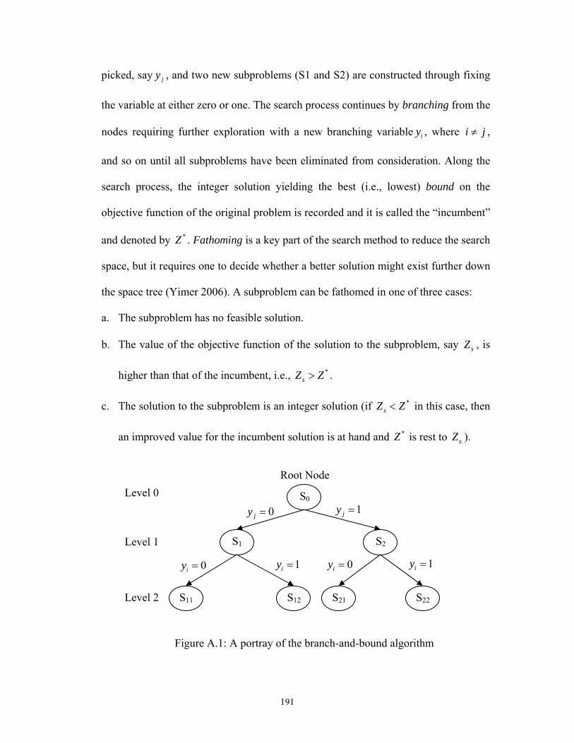
191
picked, say jy , and two new subproblems (S1 and S2) are constructed through fixing
the variable at either zero or one. The search process continues by branching from the
nodes requiring further exploration with a new branching variable iy , where i j≠ ,
and so on until all subproblems have been eliminated from consideration. Along the
search process, the integer solution yielding the best (i.e., lowest) bound on the
objective function of the original problem is recorded and it is called the “incumbent”
and denoted by *Z . Fathoming is a key part of the search method to reduce the search
space, but it requires one to decide whether a better solution might exist further down
the space tree (Yimer 2006). A subproblem can be fathomed in one of three cases:
a. The subproblem has no feasible solution.
b. The value of the objective function of the solution to the subproblem, say sZ , is
higher than that of the incumbent, i.e., *sZ Z> .
c. The solution to the subproblem is an integer solution (if *sZ Z< in this case, then
an improved value for the incumbent solution is at hand and *Z is rest to sZ ).
Figure A.1: A portray of the branch-and-bound algorithm
S0
S2
S11 S12 S21 S22
S1
0jy = 1jy =
0iy = 1iy = 0iy = 1iy =
Root NodeLevel 0
Level 1
Level 2

192
Clearly, a bound obtained at a particular node is always better or at worse the
same as that obtained at the descendent nodes of the lower level. Once there are no
more nodes to explore, the incumbent solution found so far is recorded as the optimal
solution to the original problem and the algorithm is terminated.
A.4 Benders decomposition algorithm
This technique was originally proposed by Benders (1962) for the solution of
MILP and was later extended by Geoffrion (1972) to handle MINLP through the use
of nonlinear duality theory. Since its introduction, Benders decomposition has gained
wide popularity among researchers and has been successfully applied to several
problems such as supply chain network design and reconfiguration (Osman and
Demirli 2010), multi-commodity distribution planning (Cakir 2009, Geoffrion and
Graves 1974), power flow and transmission optimization problems (Binato et al.
2001, Alguacil and Conejo 2000) among many others. A review of the applications of
Benders decomposition to the fixed charge network design problem is given by Costa
(2005).
The applicability of Benders decomposition (BD) arises mainly in mathematical
models involving complicating variables, where in most practical situations these
variables assume either integer or binary values. Basically, the idea is to decompose
the model through dealing with the complicating variables (CVs) separately into the
“master problem” (MP) and the non-complicating variables (NCVs) into the “sub-
problem” (SP). The MP is composed of the objective function terms involving the
CVs, the constraints on these variables as well as the added cuts obtained from the
solution of the SP. The values of the NCVs are optimized via solving the SP which

193
fixes the values of the CVs to those obtained via solving the MP. The dual multipliers
associated with fixed values for the CVs are obtained from the SP and are used to
construct an optimality cut that is added iteratively to the MP. After each iteration, a
convergence check is carried out on the upper and lower bounds obtained by solving
the two problems. Let us consider the following MILP involving both types of
variables (Conejo et al. 2006):
(P3) Min 1 1
n m
i i j ji j
Z c x d y= =
= +∑ ∑ (A.15)
S.t.
1 1
n m
li i lj j li j
a x e y b= =
+ ≤∑ ∑ 1,...,l q= (A.16)
down upi i ix x x≤ ≤ , ix N∈ 1, ...,i n= (A.17)
down upj j jy y y≤ ≤ , jy R∈ 1,...,j m= (A.18)
In the above model, ix is considered to be the complicating variable, which can
also be binary instead, and jy is the non-complicating variable. Note that BD is also
applicable to linear programs where the complicating variables in this case would be
those preventing the solution to the problem by blocks. The BD algorithm calls for
decomposing (P3) into the following two problems:
Master problem (MP):
Min ( )
1
nv
M P i ii
Z c x α=
= +∑ (A.19)
S.t.
( )( ) ( ) ( )
1
mk k k
j j i i ij
d y x xα λ=
≥ + −∑ 1,..., 1k v= − (A.20)

194
down upi i ix x x≤ ≤ , ix N∈ 1, ...,i n= (A.21)
downα α≥ (A.22)
Sub-problem (SP):
Min 1
m
SP j jj
Z d y=
= ∑ (A.23)
S.t.
1 1
m n
lj j l li ij i
e y b a x= =
≤ −∑ ∑ 1,...,l q= (A.24)
down upj j jy y y≤ ≤ , jy R∈ 1,...,j m= (A.25)
( )vi ix x= : iλ 1, ...,i n= (A.26)
At each iteration, a feasible solution to the SP implies an additional optimality cut
of the form (A.20) that is appended to the MP. However, for the case of binary
variables, Codato and Fischetti (2004) proposed the addition of a combinatorial
feasibility cut to the master problem after each iteration where no feasible solution to
the SP exists. The role of this cut is to force the MP to generate 0-1 values that differ
from those causing infeasibility in the previous iteration by at least one. For binary ix
variables, the feasibility cut has the general form:
( )( ) ( ): 0 : 1
1 1k k
i i
n n
i ii x i x
x x= =
+ − ≥∑ ∑ 1,..., 1k v= − (A.27)
As we proceed iteratively with the algorithm, the values of the variable α keep
on increasing, or possibly stay the same, due to the added optimality cuts after each
feasible iteration. However, the objective function of the SP might increase or
decrease depending on the values of the CVs obtained from the MP. The algorithm
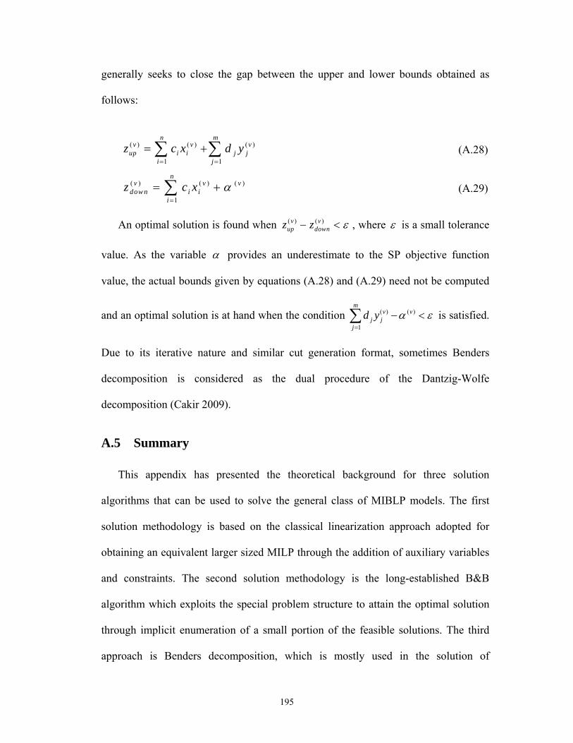
195
generally seeks to close the gap between the upper and lower bounds obtained as
follows:
( ) ( ) ( )
1 1
n mv v v
up i i j ji j
z c x d y= =
= +∑ ∑ (A.28)
( ) ( ) ( )
1
nv v v
dow n i ii
z c x α=
= +∑ (A.29)
An optimal solution is found when ( ) ( )v v
up downz z ε− < , where ε is a small tolerance
value. As the variable α provides an underestimate to the SP objective function
value, the actual bounds given by equations (A.28) and (A.29) need not be computed
and an optimal solution is at hand when the condition ( ) ( )
1
mv v
j jj
d y α ε=
− <∑ is satisfied.
Due to its iterative nature and similar cut generation format, sometimes Benders
decomposition is considered as the dual procedure of the Dantzig-Wolfe
decomposition (Cakir 2009).
A.5 Summary
This appendix has presented the theoretical background for three solution
algorithms that can be used to solve the general class of MIBLP models. The first
solution methodology is based on the classical linearization approach adopted for
obtaining an equivalent larger sized MILP through the addition of auxiliary variables
and constraints. The second solution methodology is the long-established B&B
algorithm which exploits the special problem structure to attain the optimal solution
through implicit enumeration of a small portion of the feasible solutions. The third
approach is Benders decomposition, which is mostly used in the solution of

196
mathematical models involving complicating variables. The next chapter illustrates
how such algorithms can be customized to solve the production planning problem at
hand.