Queues and risk models

Citation for published version (APA):Badila, E. S. (2015). Queues and risk models. Eindhoven: Technische Universiteit Eindhoven.

Document status and date:Published: 01/01/2015

Document Version:Publisher’s PDF, also known as Version of Record (includes final page, issue and volume numbers)

Please check the document version of this publication:

• A submitted manuscript is the version of the article upon submission and before peer-review. There can beimportant differences between the submitted version and the official published version of record. Peopleinterested in the research are advised to contact the author for the final version of the publication, or visit theDOI to the publisher's website.• The final author version and the galley proof are versions of the publication after peer review.• The final published version features the final layout of the paper including the volume, issue and pagenumbers.Link to publication

General rightsCopyright and moral rights for the publications made accessible in the public portal are retained by the authors and/or other copyright ownersand it is a condition of accessing publications that users recognise and abide by the legal requirements associated with these rights.

• Users may download and print one copy of any publication from the public portal for the purpose of private study or research. • You may not further distribute the material or use it for any profit-making activity or commercial gain • You may freely distribute the URL identifying the publication in the public portal.

If the publication is distributed under the terms of Article 25fa of the Dutch Copyright Act, indicated by the “Taverne” license above, pleasefollow below link for the End User Agreement:www.tue.nl/taverne

Take down policyIf you believe that this document breaches copyright please contact us at:openaccess@tue.nlproviding details and we will investigate your claim.

Download date: 29. Apr. 2020

Queues and Risk Models

This work is part of the research project Queues and Risk Models (QUARM 613.001.017)funded by

c© Emil Serban Badila, 2015.

Queues and Risk Models / by E.S. Badila. –

Mathematics Subject Classification (2010):Primary 60K25 (Queueing theory), 91B30 (Risk theory, Insurance),Secondary 60G51 (Processes with independent increments; Levy processes), 62P05(Applications to actuarial sciences and financial mathematics),90B22 (Queues and service).

A catalogue record is available from the Eindhoven University of Technology Library.ISBN: 978-90-386-3877-5

Printed by: Gildeprint

Queues and Risk Models

proefschrift

ter verkrijging van de graad van doctor aan deTechnische Universiteit Eindhoven, op gezag van de

rector magnificus, prof.dr.ir. F.P.T. Baaijens, voor eencommissie aangewezen door het College voor

Promoties in het openbaar te verdedigenop maandag 22 juni 2015 om 14.00 uur

door

Emil Serban Badila

geboren te Targu-Mures, Roemenie

Dit proefschrift is goedgekeurd door de promotoren en de samenstelling van depromotiecommissie is als volgt:

voorzitter: prof.dr. E.H.L. Aarts1e promotor: prof.dr.ir. O.J. Boxmaco-promotor: dr. J.A.C. Resingleden: prof.dr.ir. I.J.B.F. Adan

prof.dr. H. Albrecher (Universite de Lausanne)prof.dr. J.S.H. van Leeuwaardenprof.dr. M.R.H. Mandjes (University of Amsterdam)prof.dr. Z. Palmowski (University of Wroc law)

Acknowledgments

The contents of this book are the result of the four-year work on the topic presented inthe title. Intensive as it was, it wouldn’t have been possible without the contributionand support of many people, to whom I am most grateful.

Firstly, I am indebted to my supervisors. Onno was always kind, careful and eagerto help and inspire me with a fantastic mathematical common sense and intuition;And on top of this with a great sense of humor. I am a lucky fellow to have youas a supervisor. I want to thank Jacques for all the fruitful discussions we had.Throughout all our projects, you always managed to make the right remarks and raisejust objections, especially when I was being sloppy. When I had a question, the doorsof your offices were always open.

I would also like to thank Hansjoerg Albrecher, Zbigniew Palmowski, MichelMandjes, Ivo Adan and Johan van Leeuwaarden for agreeing to be part of thecommittee. Special thanks go to Hansjoerg for inviting me to visit his group inLausanne and to Jevgenij for taking me around the city. I also want to thank Zbyszekfor the visit I paid to Wroc law and for the good work we have done together; Thisvisit has also been a great opportunity to have some nice discussions with ThomaszRolski.

EURANDOM felt like a big family. Without trying to be precise, I witnessedhere two successive generations of PhD students. I have to mention the pleasantevenings at Botond, Robert and Elena’s house - the EURANDOM house as we usedto call it. The barbecues, the games and the pub quizzing have always been a gooddistraction. It was great to have around the ”old” bunch of jolly fellows (in randomorder): Tim, Stella, Paulo, Julia, Peter, Jan-Pieter, Eleni, Enrico, Carlo, Martin,Florence, Sander. And a special mention for Jaron whom I’ve never seen performinglive yet and Alessandro, with whom I had the trip to the other end of the world. Thenthere is the new generation; I had many nice evenings, pizzas and board games withBritt, Jori, Alessandro, Maria Luisa, Fabio, Thomas, Gianmarco, Murtaza, Szilard,Clara, Rick, Bart, Fiona and Mirko. Besides, there were also the squash and thebasketball games with Fabio. Thank you all for the great time.

v

vi Acknowledgments

I also wish to thank Razvan, Ada, Andrei, Andreea, Dragos, Ionut, Delia, Radu; Icould not write this without mentioning you here. I wish I would see you more often.

Finally, I am grateful to Maria, Daniela and to my parents for their unconditionallove and support.

Serban BadilaEindhoven, May 2015

Contents

Acknowledgments v

1 Introduction 1

1.1 Single server queues and Sparre-Andersen risk reserve processes, withcorrelations . . . . . . . . . . . . . . . . . . . . . . . . . . . . . . . . . 4

1.2 Queueing systems and risk reserve processes with multiple components 8

1.3 Duality . . . . . . . . . . . . . . . . . . . . . . . . . . . . . . . . . . . 10

1.4 Outline and contributions . . . . . . . . . . . . . . . . . . . . . . . . . 12

2 Duality 15

2.1 The embedded workload as a potential loss for the risk reserve process 16

2.2 Multivariate duality . . . . . . . . . . . . . . . . . . . . . . . . . . . . 18

2.3 Siegmund duality for coupled processors models . . . . . . . . . . . . . 21

3 Single server queues and Sparre-Andersen risk reserve processeswith correlations 31

3.1 Model description and analysis of waiting times . . . . . . . . . . . . 32

3.2 The steady-state workload . . . . . . . . . . . . . . . . . . . . . . . . . 36

3.3 Duality between the insurance and queueing processes . . . . . . . . . 38

3.4 Examples and numerical results . . . . . . . . . . . . . . . . . . . . . . 41

3.5 Appendix A . . . . . . . . . . . . . . . . . . . . . . . . . . . . . . . . . 50

4 Integral representations for one-dimensional random walks 55

4.1 On Hewitt’s inversion formula . . . . . . . . . . . . . . . . . . . . . . . 57

4.1.1 Preliminaries . . . . . . . . . . . . . . . . . . . . . . . . . . . . 57

4.2 The GI/G/1 queue with correlations . . . . . . . . . . . . . . . . . . . 61

4.2.1 The number of arrivals during an excursion . . . . . . . . . . . 66

4.3 Examples . . . . . . . . . . . . . . . . . . . . . . . . . . . . . . . . . . 68

4.4 The time to ruin when starting at a positive level . . . . . . . . . . . . 73

vii

viii Contents

5 Queues and risk processes with multivariate Poisson input 775.1 Model description . . . . . . . . . . . . . . . . . . . . . . . . . . . . . . 785.2 The analysis of the two-dimensional problem . . . . . . . . . . . . . . 795.3 Relation with other models . . . . . . . . . . . . . . . . . . . . . . . . 835.4 The k-dimensional problem . . . . . . . . . . . . . . . . . . . . . . . . 875.5 The general two-dimensional workload/reinsurance problem . . . . . . 935.6 Appendix B . . . . . . . . . . . . . . . . . . . . . . . . . . . . . . . . . 97

6 Two parallel insurance lines with simultaneous arrivals 996.1 Model description . . . . . . . . . . . . . . . . . . . . . . . . . . . . . 1006.2 A functional equation . . . . . . . . . . . . . . . . . . . . . . . . . . . 1026.3 Wiener-Hopf analysis of the stochastic recursion . . . . . . . . . . . . 104

6.3.1 Preparations . . . . . . . . . . . . . . . . . . . . . . . . . . . . 1056.3.2 A Wiener-Hopf factorization . . . . . . . . . . . . . . . . . . . 1076.3.3 The main result . . . . . . . . . . . . . . . . . . . . . . . . . . 110

6.4 A probabilistic decomposition . . . . . . . . . . . . . . . . . . . . . . . 1126.5 Examples and numerical inversion . . . . . . . . . . . . . . . . . . . . 1146.6 Appendix C . . . . . . . . . . . . . . . . . . . . . . . . . . . . . . . . . 124

7 Proportional reinsurance with subexponential claims 1277.1 Introduction . . . . . . . . . . . . . . . . . . . . . . . . . . . . . . . . . 1277.2 Main results . . . . . . . . . . . . . . . . . . . . . . . . . . . . . . . . . 1287.3 Proof of the main result . . . . . . . . . . . . . . . . . . . . . . . . . . 129

8 A coupled processor model with simultaneous arrivals 1378.1 Model description . . . . . . . . . . . . . . . . . . . . . . . . . . . . . . 1388.2 Recursive equations for the amount of work in the coupled system . . 1398.3 The transform of the equilibrium amount of work at arrival epochs . . 1418.4 The k -dimensional model . . . . . . . . . . . . . . . . . . . . . . . . . 1448.5 Conclusions and final remarks . . . . . . . . . . . . . . . . . . . . . . . 148

Bibliography 151

Summary

Curriculum Vitae

Chapter 1

Introduction

There are many daily life examples related to traffic and the problem of congestion,which occur whenever a given resource cannot keep up with the rate of arrival ofservice requests. Examples of offered resources include Internet bandwidth, the widthof a highway as part of a traffic network, the speed of the central processing unit(CPU) in a computer, or the working speed of a server at a counter in a supermarket.A natural way to mitigate the unavoidable congestion issues is to consider a bufferin which arriving customers/jobs can queue up waiting for service. The study ofphenomena related to congestion relies significantly on the mathematics of QueueingTheory, and this includes related problems such as the design and optimization ofqueueing systems. There is a dual perspective which makes queueing processes appearas mirror images of so-called risk reserve processes (or better called surplus processes).These latter describe the dynamics of the surplus process of an insurance portfolio, orthe evolution of assets on the stock market.

The amount of processing time demanded from a CPU is not constant among thevarious requested jobs. Even more so, one cannot expect fixed deterministic timepoints at which cars arrive at an intersection. Similarly, arrival epochs of accidentclaims incurred by an insurance portfolio are subject to hazard and so is their severity.Thus one is naturally led to consider the input processes in these systems as beingstochastic in nature.

Among the associated key performance measures one can think of are the waitingtime of a typical customer before receiving service, the workload demanded from theserver at any point in time, the queue length etc., and in the set-up of surplus processesone is typically interested in the ruin probability, the time to ruin and the deficit of thesurplus process at ruin. In view of the above, these performance measures are to beregarded as random variables or closely related entities, and this leads to consideringthe input in the form of a stochastic process.

The mathematical problems that appear in applications coming from queueingtheory and insurance can typically be reduced to the study of the supremum andinfimum functionals of a stochastic process, together with their associated excursionprocesses (as excursions away from the minimum). Part of the study of fluctuations isrelated to ergodic theorems that specify conditions on the traffic load under which the

1

2 Introduction

above extreme functionals converge as time goes to infinity, and respectively conditionsunder which the distribution of an excursion length is a probability distribution (whichmay be defective). By the theory of fluctuations we mean the study of these problemsand related ones, like the rate of convergence of the above functionals in the ergodiccase. These appear in many related areas of Probability and Statistics, however, froman applications point of view, the focus in this thesis will be on queueing and riskreserve processes.

There is a convenient way to talk about queues and risk reserve processes atthe same time without explicitly mentioning any of them. Let (tn)n be a countablesequence of random points on R (thought of as the time axis), and make correspond toeach point tn a random element Bn of some probability space. We will call the sequenceof tuples {(tn, Bn)}n, a marked point process (allow n ∈ Z). The first chapters arededicated to the study of marked point processes with the special feature that theinter-arrival process is renewal and in the positive flow of time, the current mark sizeis allowed to depend on the time until the next arrival epoch. The positive directionfor the time flow corresponds to queueing applications, so that if we denote the inter-arrivals by An := tn+1 − tn, the sequence {(An, Bn)}n is assumed independent andidentically distributed (i.i.d.). For the setting of risk reserve processes, the directionin which time flows is reversed so that the current mark size may depend on the timeelapsed since the previous mark epoch. The reason for changing the direction of timeis that, in some cases, queueing and surplus processes can be backwards coupled onewith another in such a way that their key performance measures can be related. Andthen the processes are said to be in duality. A special focus will be on the case whenthe point process is Poisson with the Lebesgue measure as intensity. Also of specialinterest is when the marks are random vectors. It may happen that the distributionsof the vectors of marks may be supported on proper linear subspaces of the embeddingspace. In the case of Poisson point processes, this can happen if we merge differentarrival processes that mark only proper subspaces. For example, in queueing terms,for two servers working in parallel we can have arriving customers that demand serviceonly from one of the two available servers, but there can also be customers that demandwork from both servers simultaneously. Similarly, an insurer can choose to reinsureonly part of its portfolio; so that some types of incoming risks will not be shared.

About the motivation behind this thesis, there are two main problems investigatedthat are overlapping:

1. The study of multidimensional queueing processes and insurance/risk processes.This is a difficult topic in itself and a significant part of the thesis is dedicated to itsstudy. The focus will be on calculating the stationary distribution of the maximum(under various orderings on Rn) of the vector-valued input process, under suitablestability conditions that ensure these maxima have proper distributions in the limit.Similarly as in one dimension, from the queueing perspective these are related to thevector-valued amount of work in the whole system, but the maxima also give varioustypes of ruin probabilities in the related surplus process (there are several ways inwhich ruin can occur, for example it can ultimately happen in all the components ofthe surplus process or in just one of them, etc.).

A special class of risk reserve processes is related to the so-called proportional

3

reinsurance contracts for which a generic claim (which corresponds to the marks of thearrival process) is shared by two insurance companies in fixed proportions. A relevantquestion in general and for this problem in particular is to understand the asymptoticbehaviour of the ruin probability as a function of the initial capital, for large values ofthis capital.

Another special feature in several dimensions is that the marginal processes mayinteract with each other. This is the case for the so-called coupled processor model; fortwo processors, this is an interacting queueing system in which as soon as a processorbecomes idle (the marginal amount of work hits level 0) it switches to assist the otherprocessor, if there is any work in the other buffer at this instant.

2. To try to remove, as much as possible, the requirement that the inter-arrivaltimes and the mark sizes form independent families of random variables. In manyapplications arrival patterns are sometimes periodic or they can become bursty fromtime to time. Going to the heart of the matter, the question is whether one can studyfluctuations of sums of variables that are neither independent nor stationary and evenmore, if, when dealing with such problems, one can forge weapons that are as effectiveas the Fourier transform methods that are traditionally used in the study of sums ofindependent variables.

These two topics are intertwined: in several dimensions, there are various correla-tions between the components of the vector-valued processes that are considered asinput. Without having to complicate the model by allowing the marginal systems tointeract, the possibility to have dedicated arrivals into a subset of the componentscauses correlations in the dynamics of the whole system and this is already a sourcefor many difficulties. This is the case for instance when studying networks of queuesor several insurance companies that share risks.

The second problem is relevant on its own. The assumption of renewal arrivals,which was used systematically by Pollaczek, Lindley, Kendall and many others, isappealing from a mathematical perspective because, while it generalizes the assumptionof Poisson arrivals, it is still tractable if one uses the analytic theory of Fourier(-Stieltjes)transforms and the related Laplace-Stieltjes transforms. However, the renewal structureis broken as soon as one allows the rate of the Poisson process to be time dependentor even stochastic by itself (as in a Cox process). Even more so, known measurementsof the internet traffic show that the packet sizes (these stand for the successive marksof the arrival process) are correlated with each other even at large lags (long rangedependence). Both these extensions and their associated fluctuation problems areintensively studied in the literature; they are broad research topics so we will endup barely scratching the surface and leaving many contributions unmentioned in thefollowing sections.

The rest of this chapter is organized as follows: Section 1.1 gives an overview of thesingle server queue G/G/1 with various correlation devices in the input process andthe related work in the insurance literature on the Sparre-Andersen insurance model.Section 1.2 reviews the literature on multivariate queueing systems and contributionsfrom the related insurance literature. Section 1.3 is an informal introduction to thetopic of duality and prepares the ground for Chapter 2. Finally, Section 1.4 gives anoverview of the thesis and briefly presents its main contributions.

4 Introduction

1.1 Single server queues and Sparre-Andersenrisk reserve processes, with correlations

We begin by introducing the basic queueing system, the single server queue, andthe related risk reserve process. The key performance measures that will be studiedthroughout the thesis are also introduced.

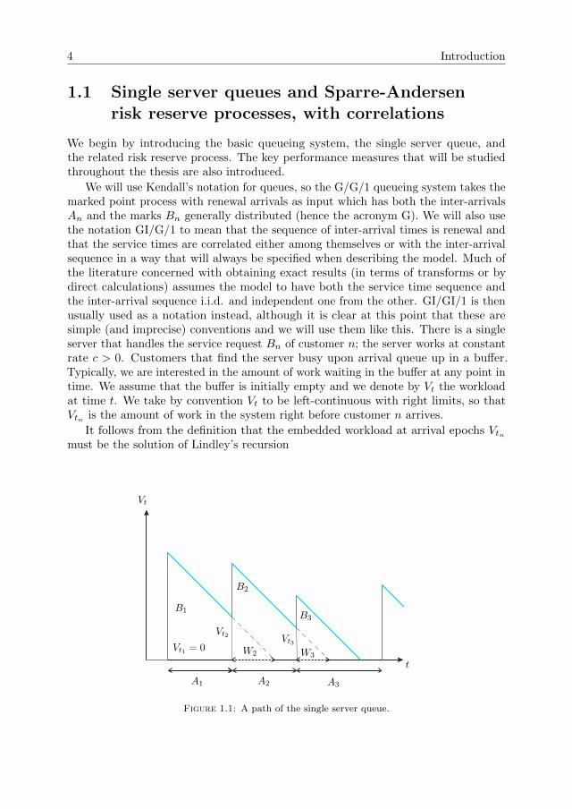
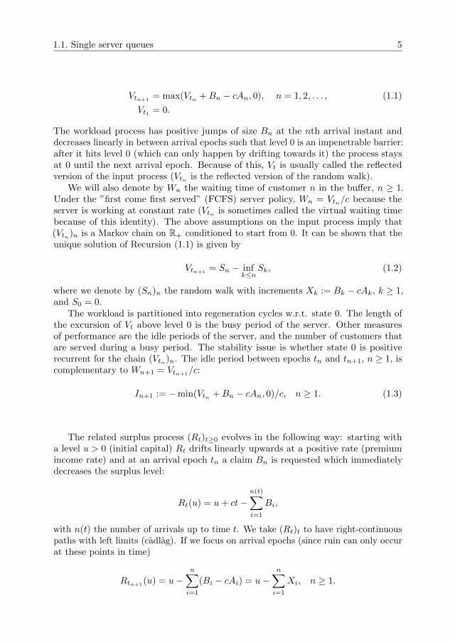
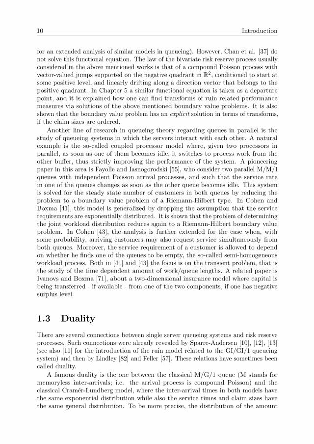
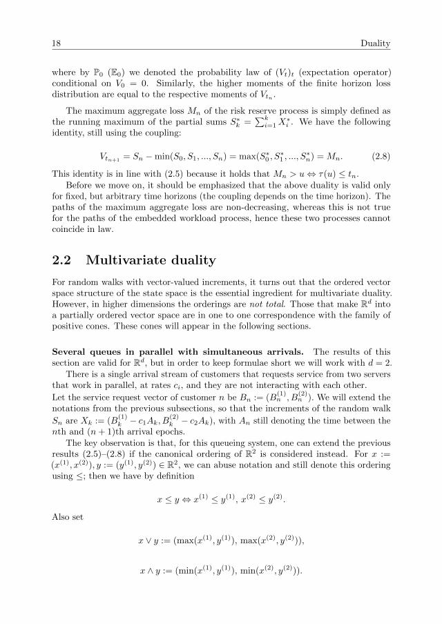
We will use Kendall’s notation for queues, so the G/G/1 queueing system takes themarked point process with renewal arrivals as input which has both the inter-arrivalsAn and the marks Bn generally distributed (hence the acronym G). We will also usethe notation GI/G/1 to mean that the sequence of inter-arrival times is renewal andthat the service times are correlated either among themselves or with the inter-arrivalsequence in a way that will always be specified when describing the model. Much ofthe literature concerned with obtaining exact results (in terms of transforms or bydirect calculations) assumes the model to have both the service time sequence andthe inter-arrival sequence i.i.d. and independent one from the other. GI/GI/1 is thenusually used as a notation instead, although it is clear at this point that these aresimple (and imprecise) conventions and we will use them like this. There is a singleserver that handles the service request Bn of customer n; the server works at constantrate c > 0. Customers that find the server busy upon arrival queue up in a buffer.Typically, we are interested in the amount of work waiting in the buffer at any point intime. We assume that the buffer is initially empty and we denote by Vt the workloadat time t. We take by convention Vt to be left-continuous with right limits, so thatVtn is the amount of work in the system right before customer n arrives.

It follows from the definition that the embedded workload at arrival epochs Vtnmust be the solution of Lindley’s recursion

Vt

B1

B2

B3

W2 W3Vt1 = 0

Vt2 Vt3

A1 A2 A3

t

1

Figure 1.1: A path of the single server queue.

1.1. Single server queues 5

Vtn+1= max(Vtn +Bn − cAn, 0), n = 1, 2, . . . , (1.1)

Vt1 = 0.

The workload process has positive jumps of size Bn at the nth arrival instant anddecreases linearly in between arrival epochs such that level 0 is an impenetrable barrier:after it hits level 0 (which can only happen by drifting towards it) the process staysat 0 until the next arrival epoch. Because of this, Vt is usually called the reflectedversion of the input process (Vtn is the reflected version of the random walk).

We will also denote by Wn the waiting time of customer n in the buffer, n ≥ 1.Under the ”first come first served” (FCFS) server policy, Wn = Vtn/c because theserver is working at constant rate (Vtn is sometimes called the virtual waiting timebecause of this identity). The above assumptions on the input process imply that(Vtn)n is a Markov chain on R+ conditioned to start from 0. It can be shown that theunique solution of Recursion (1.1) is given by

Vtn+1= Sn − inf

k≤nSk, (1.2)

where we denote by (Sn)n the random walk with increments Xk := Bk − cAk, k ≥ 1,and S0 = 0.

The workload is partitioned into regeneration cycles w.r.t. state 0. The length ofthe excursion of Vt above level 0 is the busy period of the server. Other measuresof performance are the idle periods of the server, and the number of customers thatare served during a busy period. The stability issue is whether state 0 is positiverecurrent for the chain (Vtn)n. The idle period between epochs tn and tn+1, n ≥ 1, iscomplementary to Wn+1 = Vtn+1

/c:

In+1 := −min(Vtn +Bn − cAn, 0)/c, n ≥ 1. (1.3)

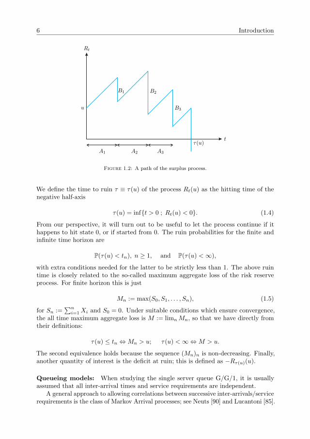
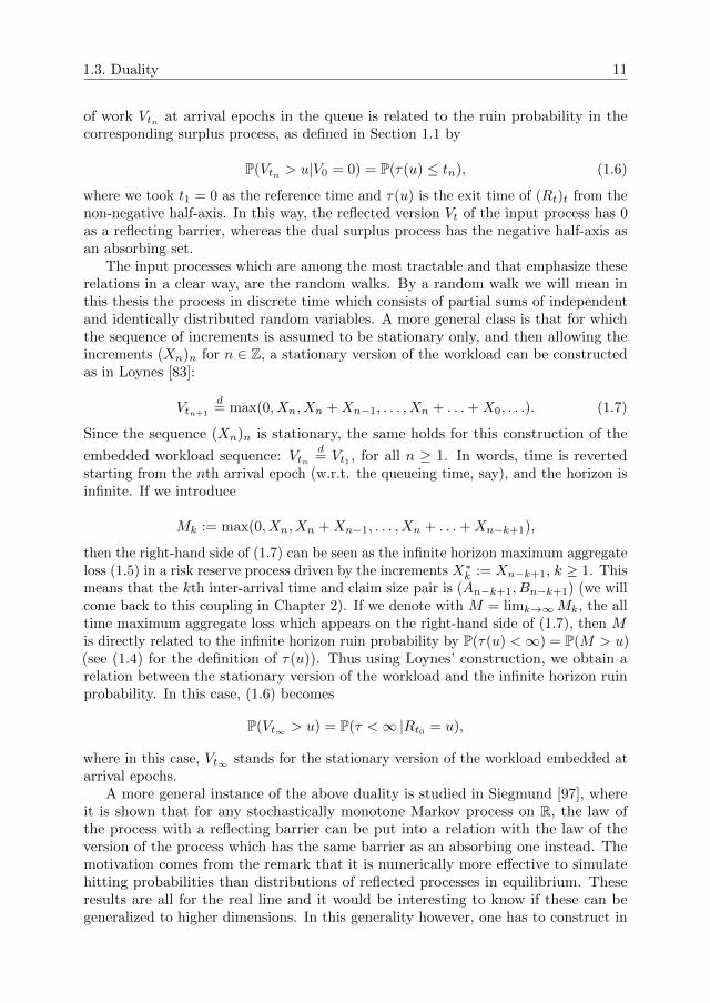
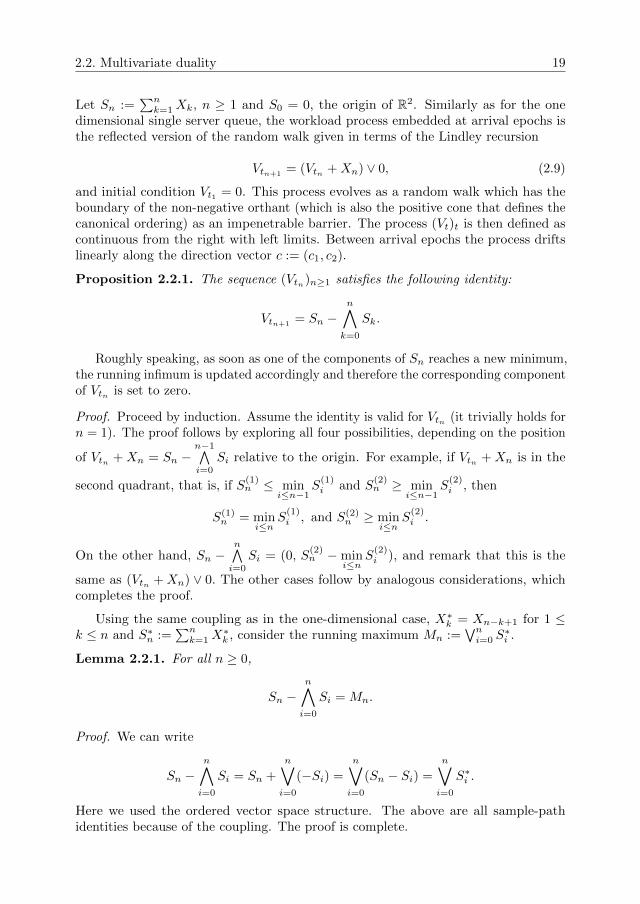
The related surplus process (Rt)t≥0 evolves in the following way: starting witha level u > 0 (initial capital) Rt drifts linearly upwards at a positive rate (premiumincome rate) and at an arrival epoch tn a claim Bn is requested which immediatelydecreases the surplus level:

Rt(u) = u+ ct−n(t)∑i=1

Bi,

with n(t) the number of arrivals up to time t. We take (Rt)t to have right-continuouspaths with left limits (cadlag). If we focus on arrival epochs (since ruin can only occurat these points in time)

Rtn+1(u) = u−n∑i=1

(Bi − cAi) = u−n∑i=1

Xi, n ≥ 1.

6 Introduction

Rt

B1 B2

B3u

τ(u)t

A1 A2 A3

1

Figure 1.2: A path of the surplus process.

We define the time to ruin τ ≡ τ(u) of the process Rt(u) as the hitting time of thenegative half-axis

τ(u) = inf{t > 0 ; Rt(u) < 0}. (1.4)

From our perspective, it will turn out to be useful to let the process continue if ithappens to hit state 0, or if started from 0. The ruin probabilities for the finite andinfinite time horizon are

P(τ(u) < tn), n ≥ 1, and P(τ(u) <∞),

with extra conditions needed for the latter to be strictly less than 1. The above ruintime is closely related to the so-called maximum aggregate loss of the risk reserveprocess. For finite horizon this is just

Mn := max(S0, S1, . . . , Sn), (1.5)

for Sn :=∑ni=1Xi and S0 = 0. Under suitable conditions which ensure convergence,

the all time maximum aggregate loss is M := limnMn, so that we have directly fromtheir definitions:

τ(u) ≤ tn ⇔Mn > u; τ(u) <∞⇔M > u.

The second equivalence holds because the sequence (Mn)n is non-decreasing. Finally,another quantity of interest is the deficit at ruin; this is defined as −Rτ(u)(u).

Queueing models: When studying the single server queue G/G/1, it is usuallyassumed that all inter-arrival times and service requirements are independent.

A general approach to allowing correlations between successive inter-arrivals/servicerequirements is the class of Markov Arrival processes; see Neuts [90] and Lucantoni [85].

1.1. Single server queues 7

Phase-type inter-arrivals and Markov-Modulated Poisson arrival processes are con-tained in this class.

Following Lucantoni [85], a natural way of correlating inter-arrivals with mark sizesis the Batch Markov Arrival Process (BMAP) and its associated queueing system,the BMAP/G/1 queue, where the arrival of a batch of size k ≥ 1 causes the requestto process k i.i.d. service components, each having some generally distributed size.The BMAP/G/1 queue provides a versatile framework to model dependence betweensuccessive inter-arrival times but also dependence between inter-arrival times andservice requirements. In Combe and Boxma [45] the BMAP is also used to studyan M/G/1 queue in which service requirements depend on the previous inter-arrivaltimes; see Borst et al. [33] for a different approach to the latter form of dependence,which does not use the MAP machinery.

An important paper regarding dependence between inter-arrival and service re-quirements is the one by Adan and Kulkarni [2]. They consider a single server queuewith Markov-dependent inter-arrival and service requirements: a service requirementand subsequent inter-arrival time have a bivariate distribution that depends on anunderlying Markov chain which jumps at customer arrival epochs. The inter-arrivaltimes in [2] are exponentially distributed, with rate λj when the Markov chain jumpsto state j. See also Constantinescu et al. [48], where a different approach is used tostudy similar models for the risk reserve process. The methods used therein are basedon operator theory (Heaviside operational calculus).

It should be observed that the analysis of a GI/G/1 queue with some dependencestructure between a service requirement Bi and the subsequent inter-arrival time Aiis intrinsically easier than that of a GI/G/1 queue with some dependence structurebetween Ai and the next Bi+1. The reason is that Bi and Ai only appear as a differencein the Lindley recursion (1.1) for the waiting time Wi of the ith arriving customer.In Chapter 3 we will study the problem of fluctuations of a queue which has matrixexponential service requirements (see Bladt and Nielsen [29]) that are also correlatedwith subsequent inter-arrival times. The working assumption is given in terms of theLaplace-Stieltjes transform of the vector composed of the inter-arrival time togetherwith the corresponding service requirement, namely, it is assumed that this is a rationalfunction in both arguments. The classes of phase-type random vectors known in theliterature as Assaf’s [18] or Kulkarni’s [79] are special instances. This class allows usto obtain detailed, explicit, results for the steady-state waiting time, workload and idleperiod, and even to stochastically compare the waiting time distributions for varioustypes of correlation.

By focusing on the arrival instants of marks, the study of the waiting time andidle time distribution in the GI/G/1 queue reduces to the study of a random walkwith increments that have a rational characteristic function and can thus be continuedanalytically in the whole plane except for a finite number of poles.

Insurance risk: Having discussed the queueing literature with dependence betweeninter-arrival time and service requirement, let us now turn to the insurance riskliterature with dependence between inter-claim time and claim size. In recent years,this has been a hot topic in risk theory. Albrecher and Boxma [4] derive exact formulasfor the ruin probability in a Cramer-Lundberg model with a threshold-type dependence

8 Introduction

between a claim size and the next inter-claim time. In Albrecher and Boxma [5] amuch more general semi-Markovian risk model is being considered, which bears someresemblance to the queueing model in Adan and Kulkarni [2]. Kwan and Yang [80]consider a specific threshold-type dependence of claim size on previous inter-claim time;in Albrecher et al. [6] this is put in the larger framework of Markov Additive Processes.Another specific dependence structure between claim size and previous inter-claim timeis treated in Boudreault et al. [34], where it is assumed that the conditional density of aclaim, given the previous inter-arrival is a mixture of two arbitrary probability densityfunctions. Asymptotic results were obtained in Albrecher and Kantor [7], where therelation between the dependence structure and the Lundberg exponent is studied. AlsoAlbrecher and Teugels [8] give asymptotic results for the finite and infinite horizonruin probabilities when the current claim size and the previous inter-claim time aredependent according to an arbitrary copula structure.

1.2 Queueing systems and risk reserve processeswith multiple components

An important part of the thesis is dedicated to the study of multidimensional queueingsystems and the related risk reserve processes. In particular, we look into the possibilityof extending the duality of Siegmund [97] to processes on higher dimensional statespaces. First, we will focus on queueing models which have a compound Poisson inputprocess with a negative drift and their dual insurance risk counterparts which take asimilar compound Poisson input with a positive drift. The negative/positive drift is interms of the componentwise ordering of Rn.

Queueing models with several queues in parallel and with an arrival process inwhich there may be simultaneous arrivals - often called fork-join queues - have manyapplications in computer-, communication- and production systems. These are modelswhere jobs are split among a number of different processors, communication channelsor machines. The servers work in parallel and each has its own dedicated buffer wherejobs wait to be processed. Clearly, the queues in these models are dependent due tothe simultaneous arrivals. In general this makes an exact analysis of the model verydifficult, and by exact analysis is meant the derivation of (Laplace-Stieltjes transformsfor) the distributions of the relevant performance measures. Only in the case oftwo queues, exact results are available; see, e.g., Flatto and Hahn [59], Wright [105],Baccelli [21], De Klein [76] and Cohen [43]. An early paper, classical for the use ofcomplex functions and singular integrals in queueing theory, is Pollaczek’s [92]. Theabove mentioned works rely heavily on advanced complex function theory, includingthe theory of boundary value problems. This not only makes the methods involved,it is often difficult to recognize the stochastic nature of the initial problem in themanipulations. It comes as no surprise that approximations and asymptotic studies aremore popular than exact methods for these multidimensional models. Given that it isstill imperative to understand fluctuation theory in higher dimensions, a starting pointwould be to understand how one can leverage the stochastic nature of the problem toactually guide the analysis (complex as it may be).

For the model with more than two servers no exact analytical results are available

1.2. Queueing systems and risk reserve processes with multiple components 9

in the literature. In this case, bounds and approximations for several performancemeasures have been developed, see e.g. Baccelli et al. [22] and Nelson and Tantawi[88, 89].

Studies of multidimensional risk reserve processes are scarce in the insuranceliterature, although results about risk measures related to such models are highlyrelevant both from a theoretical and a practitioner’s perspective. Multivariate ruinproblems are relevant because they give insight into the behaviour of risk measuresunder various types of correlations between the insurance lines. Like in queueingtheory, it is natural to study insurance risk processes with simultaneous arrivals ofclaims in several insurance lines. One example is presented by multiple insurancelines within the same company which are interacting with each other as they evolvein time, via, say, coupled income rates. Another typical example is an umbrellatype of insurance model, where a claim occurrence event generates multiple types ofclaims which may be correlated, and each type of claim is paid from its correspondingcomponent, such as car insurance together with health insurance or insurance againstearthquakes. Yet another class of models is related to reinsurance problems, where aclaim is shared between the insurer and one or more reinsurers.

Avram et al. [19, 20] have studied the joint ruin problem for the special case ofproportional reinsurance. In particular, they derive the double Laplace transform withrespect to the two initial reserves of the survival probabilities of the two companies.One of the key observations in [19, 20] is that, due to the fact that companies divideclaims in some specific proportions, the two-dimensional ruin problem may be viewedas a one-dimensional crossing problem over a piecewise linear barrier. Badescu etal. [23] have extended the two-dimensional model of [19, 20] by allowing, next tothe arrivals of claims for which the two insurers divide the claim in some specificproportions, also extra arrivals of claims which are fully paid by one of the insurers (e.g.,insurer 1). They show that under some conditions also in this model the previouslymentioned reduction to a one dimensional problem still holds. However, in [23] theauthors do not consider the double Laplace transform with respect to the two initialreserves of the survival probabilities of the two companies (their main focus is on theLaplace transform of the time until ruin of at least one insurer).

An early study of multivariate risk measures can be found in the paper of Sundt [101]about developing multivariate Panjer recursions which are then used to compute thedistribution of the aggregate claim process, assuming simultaneous claim events anddiscrete claim sizes. Other approaches are deriving integro-differential equations forthe various measures of risk and then iterating these equations to find numericalapproximations as in Chan et al. [37] and Gong et al. [67], or computing bounds forthe different types of ruin probabilities that can occur in a setting where more than oneinsurance line is considered (see Cai and Li [36] who consider multivariate phase-typeclaims). It is worth mentioning that very few papers (like Avram et al. [19], Badescuet al. [23]), analytically determine, e.g., the ruin probability for insurance models withmore than one company (see also [17], Ch. XIII.9 for an overview of this topic).

In an attempt to solve the integro-differential equations that arise from such models,Chan et al. [37] derive a Riemann-Hilbert boundary value problem for the bivariateLaplace transform of the joint survival function (see Section 5.5 for details about suchproblems arising in the context of risk and queueing theory and Cohen and Boxma [41]

10 Introduction

for an extended analysis of similar models in queueing). However, Chan et al. [37] donot solve this functional equation. The law of the bivariate risk reserve process usuallyconsidered in the above mentioned works is that of a compound Poisson process withvector-valued jumps supported on the negative quadrant in R2, conditioned to start atsome positive level, and linearly drifting along a direction vector that belongs to thepositive quadrant. In Chapter 5 a similar functional equation is taken as a departurepoint, and it is explained how one can find transforms of ruin related performancemeasures via solutions of the above mentioned boundary value problems. It is alsoshown that the boundary value problem has an explicit solution in terms of transforms,if the claim sizes are ordered.

Another line of research in queueing theory regarding queues in parallel is thestudy of queueing systems in which the servers interact with each other. A naturalexample is the so-called coupled processor model where, given two processors inparallel, as soon as one of them becomes idle, it switches to process work from theother buffer, thus strictly improving the performance of the system. A pioneeringpaper in this area is Fayolle and Iasnogorodski [55], who consider two parallel M/M/1queues with independent Poisson arrival processes, and such that the service ratein one of the queues changes as soon as the other queue becomes idle. This systemis solved for the steady state number of customers in both queues by reducing theproblem to a boundary value problem of a Riemann-Hilbert type. In Cohen andBoxma [41], this model is generalized by dropping the assumption that the servicerequirements are exponentially distributed. It is shown that the problem of determiningthe joint workload distribution reduces again to a Riemann-Hilbert boundary valueproblem. In Cohen [43], the analysis is further extended for the case when, withsome probability, arriving customers may also request service simultaneously fromboth queues. Moreover, the service requirement of a customer is allowed to dependon whether he finds one of the queues to be empty, the so-called semi-homogeneousworkload process. Both in [41] and [43] the focus is on the transient problem, that isthe study of the time dependent amount of work/queue lengths. A related paper isIvanovs and Boxma [71], about a two-dimensional insurance model where capital isbeing transferred - if available - from one of the two components, if one has negativesurplus level.

1.3 Duality

There are several connections between single server queueing systems and risk reserveprocesses. Such connections were already revealed by Sparre-Andersen [10], [12], [13](see also [11] for the introduction of the ruin model related to the GI/GI/1 queueingsystem) and then by Lindley [82] and Feller [57]. These relations have sometimes beencalled duality.

A famous duality is the one between the classical M/G/1 queue (M stands formemoryless inter-arrivals; i.e. the arrival process is compound Poisson) and theclassical Cramer-Lundberg model, where the inter-arrival times in both models havethe same exponential distribution while also the service times and claim sizes havethe same general distribution. To be more precise, the distribution of the amount

1.3. Duality 11

of work Vtn at arrival epochs in the queue is related to the ruin probability in thecorresponding surplus process, as defined in Section 1.1 by

P(Vtn > u|V0 = 0) = P(τ(u) ≤ tn), (1.6)

where we took t1 = 0 as the reference time and τ(u) is the exit time of (Rt)t from thenon-negative half-axis. In this way, the reflected version Vt of the input process has 0as a reflecting barrier, whereas the dual surplus process has the negative half-axis asan absorbing set.

The input processes which are among the most tractable and that emphasize theserelations in a clear way, are the random walks. By a random walk we will mean inthis thesis the process in discrete time which consists of partial sums of independentand identically distributed random variables. A more general class is that for whichthe sequence of increments is assumed to be stationary only, and then allowing theincrements (Xn)n for n ∈ Z, a stationary version of the workload can be constructedas in Loynes [83]:

Vtn+1

d= max(0, Xn, Xn +Xn−1, . . . , Xn + . . .+X0, . . .). (1.7)

Since the sequence (Xn)n is stationary, the same holds for this construction of the

embedded workload sequence: Vtnd= Vt1 , for all n ≥ 1. In words, time is reverted

starting from the nth arrival epoch (w.r.t. the queueing time, say), and the horizon isinfinite. If we introduce

Mk := max(0, Xn, Xn +Xn−1, . . . , Xn + . . .+Xn−k+1),

then the right-hand side of (1.7) can be seen as the infinite horizon maximum aggregateloss (1.5) in a risk reserve process driven by the increments X∗k := Xn−k+1, k ≥ 1. Thismeans that the kth inter-arrival time and claim size pair is (An−k+1, Bn−k+1) (we willcome back to this coupling in Chapter 2). If we denote with M = limk→∞Mk, the alltime maximum aggregate loss which appears on the right-hand side of (1.7), then Mis directly related to the infinite horizon ruin probability by P(τ(u) <∞) = P(M > u)(see (1.4) for the definition of τ(u)). Thus using Loynes’ construction, we obtain arelation between the stationary version of the workload and the infinite horizon ruinprobability. In this case, (1.6) becomes

P(Vt∞ > u) = P(τ <∞|Rt0 = u),

where in this case, Vt∞ stands for the stationary version of the workload embedded atarrival epochs.

A more general instance of the above duality is studied in Siegmund [97], whereit is shown that for any stochastically monotone Markov process on R, the law ofthe process with a reflecting barrier can be put into a relation with the law of theversion of the process which has the same barrier as an absorbing one instead. Themotivation comes from the remark that it is numerically more effective to simulatehitting probabilities than distributions of reflected processes in equilibrium. Theseresults are all for the real line and it would be interesting to know if these can begeneralized to higher dimensions. In this generality however, one has to construct in

12 Introduction

a case by case fashion the transition probabilities of the dual process, and this canbecome complicated in some cases. See Asmussen [15], [16], Ch. XI.2, for dualityextended to Markov modulated processes as well, and [15] for several open problems.

Another type of duality is obtained by simply changing the sign of the incrementsXn. In terms of the input processes, the inter-arrival times in the queueing systemwill correspond to claim sizes in the risk reserve process, and the service requirementsof customers become inter-arrival times for the surplus process. For example, thestandard Cramer-Lundberg model that consists of a Poisson arrival process and i.i.d.generally distributed claims is obtained from the G/M/1 queueing model (whereasthe previously discussed duality linked it to the M/G/1 queue).

This duality with the G/M/1 queue is useful because it relates performancemeasures other than the workload/maximum aggregate loss; for example, the lengthof a busy period (the excursion away from the infimum) jointly with the number ofcustomers served during this period in the single server queue corresponds under thistype of duality to the time to ruin in the risk reserve jointly with the number of claimspaid up to this time. In addition, the length of the idle period during a busy cyclerelates to the deficit at ruin of the risk reserve process: (−Rτ ). This relation waspointed out already in Prabhu [93] and the references therein; see also Frostig [64] andLopker and Perry [84].

1.4 Outline and contributions

The thesis is structured in the following way: In Chapter 2, we extend the dualityrelation in the sense of Siegmund [97], as introduced in the first part of the previoussection, to several multidimensional queueing systems with parallel servers with andwithout interactions, which will enable us to relate them to risk reserve processes withmultiple branches. The existence of interactions between the servers (the coupledprocessor model) is changing the geometry of the absorbing sets of the dual processes.Key for this type of duality is the possibility to realize the state space as an orderedvector space.

In Chapter 3 we study the GI/G/1 queue which has the current service timecorrelated with the time until the next arrival epoch. At the same time we will considerthe dual Sparre-Andersen insurance model. The focus here will be on calculating thewaiting time distribution and the idle period, which is done under the assumptionthat the distribution of the inter-arrivals jointly with the service requirements isbivariate matrix exponential – see Bladt and Nielsen [29]. By duality, the waiting timecorresponds to the ruin probability of the risk reserve process which has the currentclaim size correlated with the time elapsed since the previous arrival epoch. We alsoexplore the relation between the stationary workload and the stationary waiting time.It is shown that this relation is analogous to the one that connects the ruin probabilityfor the delayed risk reserve process and the ruin probability for the ordinary risk reserveprocess. By definition, the delayed risk reserve process has the first arrival epochdistributed as the forward recurrence time of a typical inter-arrival (the renewal arrivalprocess is started in stationarity). The ordinary risk reserve process has the samedistribution of the first inter-arrival time as the subsequent inter-arrival times (this is a

1.4. Outline and contributions 13

version of the risk reserve process conditional on an arrival happening at time 0). Theresults obtained give insight into the effect of the correlation between inter-arrivals andservice requirements/claim sizes. It is shown that a negative correlation increases thewaiting time distribution/ruin probability and a positive correlation decreases theseperformance measures when compared to independent input. The increase/decreaseare both in the sense of convex ordering (see Stoyan [100], Ch. 1).

In Chapter 4, we continue with the set-up of the random walk with scalar incrementsbut this time we study it in greater generality. The structure of the increment is stillgiven as the difference of marginals of a sample from (A,B). Without making anyassumptions on the distribution of the pair (A,B), we obtain integral representationsfor the busy period, idle period and workload in the underlying queueing model.These are obtained by generalising a well known relation that represents functionals ofprobability distributions in terms of their characteristic functions (Hewitt’s inversionformula [69]). Obtaining the above mentioned representations is equivalent to solvinga special kind of Riemann boundary value problem for the imaginary axis (this isrelated to what is usually called the Wiener-Hopf factorization in the probabilityliterature). By virtue of the duality relation described at the end of Section 1.3, theintegral representations are also valid in the context of ruin, because the busy periodcorresponds to the time to ruin and the idle period to the deficit at ruin in the dualrisk reserve process. If the two-dimensional Laplace-Stieltjes transform of the pair(A,B) is a rational function in at least one of its arguments, then the transforms ofthese performance measures can be evaluated explicitly, by contour integration.

In Chapter 5, we study a two dimensional queueing system composed of two parallelprocessors which receive input according to a compound Poisson arrival process, withsimultaneous arrivals. We show that under ordered service times, the steady stateworkload has an explicit form, and moreover a stochastic decomposition holds insteady state, which can be interpreted probabilistically in terms of the busy periods ofone of the processors (the excursion lengths of the compound Poisson process above itssuccessive minima). The results are further extended to k processors in parallel. Wealso explain how the more general problem, without the ordering assumption, can berelated to the theory of boundary value problems and singular integrals. By virtue ofresults from the multivariate duality which is discussed in Section 2.2, the distributionof the steady state waiting time vector is related to the ruin probability as a functionof the initial vector of starting capital levels in the risk reserve process.

The Poisson arrival assumption is generalized in Chapter 6, allowing for a two-dimensional renewal arrival process with general inter-arrivals which may also becoupled with the corresponding two-dimensional mark size. In this way, we extendthe BMAP set-up of Chapter 3 to two dimensions. Using the duality relations fromChapter 2, the results obtained also give the ruin probability for two-dimensional riskreserve processes, as a function of two arguments which represent the starting capitalin both marginal risk reserve processes. As a particularly important example, the ruinprobability for proportional reinsurance contracts is obtained.

The asymptotic behaviour of the ruin function for the proportional reinsuranceprocess is studied in Chapter 7, assuming that the common claim distribution that isbeing partitioned belongs to the class of subexponential distributions (long-tailed),see Foss et al. [60]. This is carried out using only probabilistic methods.

14 Introduction

Chapter 8 is dedicated to the study of two coupled processors. The focus here ison the stationary workload in the system. It is shown that if the service time vectoris ordered, the amount of work in this model can be related to the amount of workfor two parallel processors without coupling, and thus the stability condition and thesteady-state waiting time follow from the results of Chapter 5. Then the results areextended to several coupled processors.

Remark. The results of Chapter 3 are published in [24]; Chapters 5, 6, and 8 arepublished in [25], [26] and [27], respectively. Chapter 7 is part of an ongoing projecttogether with Sergey Foss, Zbigniew Palmowski and Tomasz Rolski. Finally, Chapter 4has not yet been submitted for publication.

Chapter 2

Duality

In Section 1.3 we pointed out that there is a duality relation between single serverqueues and risk reserve processes that involves time reversion. In the present chapterwe will build on this (Section 2.1) and we shall explore this type of duality betweenqueueing systems and risk reserve processes in more depth, with a special focus onmultivariate models. In Section 2.2 we present the standard model for d queues inparallel with correlated service requirements and show that this model has a dual riskreserve process that consists of d insurance companies which receive correlated claims.In Section 2.3 it is proven that there exists a duality relation which connects the twocoupled processors model (an interacting system of queues) to an absorbing processwhich has a certain open convex subset of the plane as the absorbing domain. This isthen used to derive stability conditions for the queueing system.

For a random walk (Sn)n, the duality frequently used in this thesis relies on thefact that the reflected version of Sn (the solution of (1.1)) is the same as the supremumof the time-reversed walk:

Sn − inf0≤k≤n

Sk = sup0≤k≤n

S∗k ,

where S∗k := Sn − Sn−k , for a fixed epoch n > 0 and 0 ≤ k ≤ n. This will be used torelate the amount of work in a queue to the probability of ruin in a correspondingrisk reserve process, similarly as in (1.6). We will prove this in the more general casewhen (Sn)n≥0 is vector-valued, in which case one can still construct a dual risk reserveprocess by using geometric arguments.

This type of duality can be argued with the help of a coupling, as in Asmussen [15].As in Chapter 1, let Xj := Bj − cAj be the increments that determine (Vtj )j via (1.1).For fixed n ≥ 1 and (X1, . . . , Xn) the sample vector of the increments up to time n,take the input in the risk reserve process as (X∗1 , . . . , X

∗n) where X∗j = Xn−j+1, so

that the backwards coupled risk reserve process is given by definition as

Rt∗k+1(u) = u−

k∑j=1

X∗j , 0 ≤ k ≤ n, (2.1)

15

16 Duality

with the time reversed epochs t∗k := tn − tn−k+1 and t1 = 0. This determines theentire risk reserve process (Rt)t, because in between the arrival epochs t∗k it driftslinearly upwards at constant rate c. We will investigate this coupling in more detailand derive some first consequences.

2.1 The embedded workload as a potential loss forthe risk reserve process

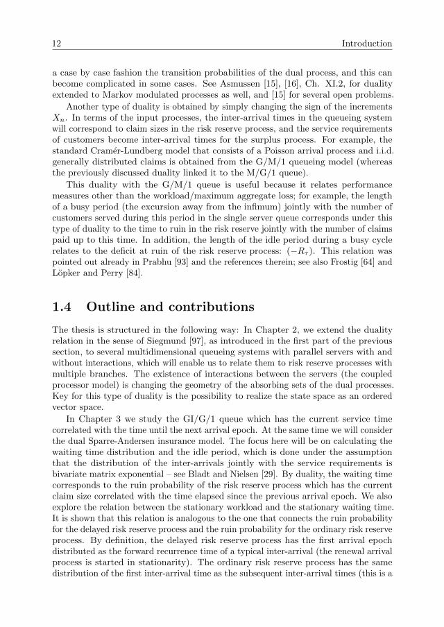
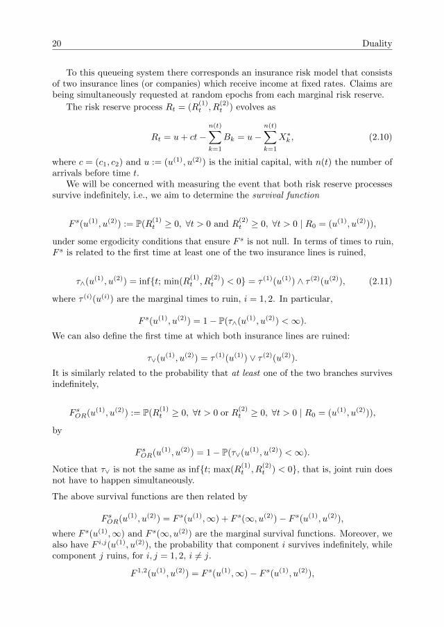
The workload process was defined below (1.1) to be right-continuous with left limits.The dual reserve process (Rt)t is defined by time reversion starting from a fixedarrival epoch tn of Vt, so that (Rt)t has cadlag paths. The following relation is afirst consequence of the above coupling. It expresses the reserve level in terms of(differences of) the embedded workload process and the idle periods In, which aredefined in (1.3).

Proposition 2.1.1. For a fixed epoch tn it holds that

Rt∗k+1(u) = u+

n∑j=n−k+1

cIj+1 −n∑

j=n−k+1

(Vtj+1− Vtj ), 0 ≤ k ≤ n, (2.2)

Proof. The differences of Vtj are related to the backwards accumulated idle period:

Vtn+1− Vtn−k+1

=

n∑j=n−k+1

Xj +

n+1∑j=n−k+2

cIj , 1 ≤ k ≤ n. (2.3)

To show this, notice that it follows at once from (1.1) and (1.3) that

Vtj+1− Vtj = Xj + cIj+1, j ≥ 1.

Then (2.3) is obtained by summing these differences for n− k + 1 ≤ j ≤ n. Replacing(2.3) in (2.1) via the coupling X∗j = Xn−j+1 obtains (2.2). The proof is complete.

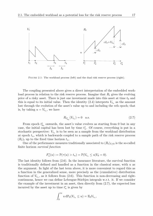
See Figure 2.1 for a coupled sample path of Vt and Rt with n = 3. For thistrajectory, I2 = 0 because Vt2 > 0.

Consider tk0 to be the last arrival epoch before tn such that Vtk0 = 0 (think interms of regeneration cycles for the workload). If nowhere sooner, then k0 = 1 andwith this choice, the backwards accumulated idle period appearing on the right-handside of (2.2) is null, hence

Rt∗k0(u) = u− Vtn+1

. (2.4)

From this follows immediately that for fixed u and a time horizon tn(= t∗n),

{Vtn > u} = {τ(u) ≤ tn}, (2.5)

with τ(u) the time to ruin as defined in Section 1.4. In terms of probabilities, we have

P(Vtn > u |V0 = 0) = P(∃τ(u) ≤ tn : Rτ(u) < 0 |R0 = u). (2.6)

2.1. The embedded workload as a potential loss for the risk reserve process 17

cI3cI3+Vt2

cI4

t∗1 t∗2 t∗3 t∗4

u

RtVt

t1 t2 t3 t4

I3 I4

1

Figure 2.1: The workload process (left) and the dual risk reserve process (right).

The coupling presented above gives a direct interpretation of the embedded work-load process in relation to the risk reserve process. Imagine that Rt gives the evolvingprice of a risky asset. There is just one investment made into this asset at time t0 andthis is equal to its initial value. Then the identity (2.4) interprets Vtn as the amountlost through the evolution of the asset’s value up to and including the nth epoch; thatis, by taking u = Vtn , we have

Rt∗k0(Vtn) = 0 a.s. (2.7)

From epoch t∗k0 onwards, the asset’s value evolves as starting from 0 but in anycase, the initial capital has been lost by time t∗n. Of course, everything is put in astochastic perspective: Vtn is to be seen as a sample from the workload distributionat epoch tn, which is backwards coupled to a sample path of the risk reserve process(Rt)t up to the fixed time horizon tn.

One of the performance measures traditionally associated to (Rt)t≥0 is the so-calledfinite horizon survival function

F sn(u) := P(τ(u) > tn) = P(Vtn ≤ u|V0 = 0).

The last identity follows from (2.6). In the insurance literature, the survival functionis traditionally defined and handled as a function in the classical sense, with u asthe argument. In light of the last term above, it is more convenient to regard this asa function in the generalized sense, more precisely as the (cumulative) distributionfunction of Vtn , as it follows from (2.6). This function is non-decreasing and right-continuous, hence we can define Lebesgue-Stieltjes integrals w.r.t. it. If we considerthe example of the investment in an asset, then directly from (2.7), the expected lossincurred by the asset up to time t∗n is given by∫ ∞

0

udP0(Vtn ≤ u) = E0Vtn ,

18 Duality

where by P0 (E0) we denoted the probability law of (Vt)t (expectation operator)conditional on V0 = 0. Similarly, the higher moments of the finite horizon lossdistribution are equal to the respective moments of Vtn .

The maximum aggregate loss Mn of the risk reserve process is simply defined asthe running maximum of the partial sums S∗k =

∑ki=1X

∗i . We have the following

identity, still using the coupling:

Vtn+1 = Sn −min(S0, S1, ..., Sn) = max(S∗0 , S∗1 , ..., S

∗n) = Mn. (2.8)

This identity is in line with (2.5) because it holds that Mn > u⇔ τ(u) ≤ tn.Before we move on, it should be emphasized that the above duality is valid only

for fixed, but arbitrary time horizons (the coupling depends on the time horizon). Thepaths of the maximum aggregate loss are non-decreasing, whereas this is not truefor the paths of the embedded workload process, hence these two processes cannotcoincide in law.

2.2 Multivariate duality

For random walks with vector-valued increments, it turns out that the ordered vectorspace structure of the state space is the essential ingredient for multivariate duality.However, in higher dimensions the orderings are not total. Those that make Rd intoa partially ordered vector space are in one to one correspondence with the family ofpositive cones. These cones will appear in the following sections.

Several queues in parallel with simultaneous arrivals. The results of thissection are valid for Rd, but in order to keep formulae short we will work with d = 2.

There is a single arrival stream of customers that requests service from two serversthat work in parallel, at rates ci, and they are not interacting with each other.

Let the service request vector of customer n be Bn := (B(1)n , B

(2)n ). We will extend the

notations from the previous subsections, so that the increments of the random walk

Sn are Xk := (B(1)k − c1Ak, B

(2)k − c2Ak), with An still denoting the time between the

nth and (n+ 1)th arrival epochs.The key observation is that, for this queueing system, one can extend the previous

results (2.5)–(2.8) if the canonical ordering of R2 is considered instead. For x :=(x(1), x(2)), y := (y(1), y(2)) ∈ R2, we can abuse notation and still denote this orderingusing ≤; then we have by definition

x ≤ y ⇔ x(1) ≤ y(1), x(2) ≤ y(2).

Also set

x ∨ y := (max(x(1), y(1)), max(x(2), y(2))),

x ∧ y := (min(x(1), y(1)), min(x(2), y(2))).

2.2. Multivariate duality 19

Let Sn :=∑nk=1Xk, n ≥ 1 and S0 = 0, the origin of R2. Similarly as for the one

dimensional single server queue, the workload process embedded at arrival epochs isthe reflected version of the random walk given in terms of the Lindley recursion

Vtn+1 = (Vtn +Xn) ∨ 0, (2.9)

and initial condition Vt1 = 0. This process evolves as a random walk which has theboundary of the non-negative orthant (which is also the positive cone that defines thecanonical ordering) as an impenetrable barrier. The process (Vt)t is then defined ascontinuous from the right with left limits. Between arrival epochs the process driftslinearly along the direction vector c := (c1, c2).

Proposition 2.2.1. The sequence (Vtn)n≥1 satisfies the following identity:

Vtn+1= Sn −

n∧k=0

Sk.

Roughly speaking, as soon as one of the components of Sn reaches a new minimum,the running infimum is updated accordingly and therefore the corresponding componentof Vtn is set to zero.

Proof. Proceed by induction. Assume the identity is valid for Vtn (it trivially holds forn = 1). The proof follows by exploring all four possibilities, depending on the position

of Vtn +Xn = Sn −n−1∧i=0

Si relative to the origin. For example, if Vtn +Xn is in the

second quadrant, that is, if S(1)n ≤ min

i≤n−1S

(1)i and S

(2)n ≥ min

i≤n−1S

(2)i , then

S(1)n = min

i≤nS

(1)i , and S(2)

n ≥ mini≤n

S(2)i .

On the other hand, Sn −n∧i=0

Si = (0, S(2)n − min

i≤nS

(2)i ), and remark that this is the

same as (Vtn +Xn) ∨ 0. The other cases follow by analogous considerations, whichcompletes the proof.

Using the same coupling as in the one-dimensional case, X∗k = Xn−k+1 for 1 ≤k ≤ n and S∗n :=

∑nk=1X

∗k , consider the running maximum Mn :=

∨ni=0 S

∗i .

Lemma 2.2.1. For all n ≥ 0,

Sn −n∧i=0

Si = Mn.

Proof. We can write

Sn −n∧i=0

Si = Sn +

n∨i=0

(−Si) =

n∨i=0

(Sn − Si) =

n∨i=0

S∗i .

Here we used the ordered vector space structure. The above are all sample-pathidentities because of the coupling. The proof is complete.

20 Duality

To this queueing system there corresponds an insurance risk model that consistsof two insurance lines (or companies) which receive income at fixed rates. Claims arebeing simultaneously requested at random epochs from each marginal risk reserve.

The risk reserve process Rt = (R(1)t , R

(2)t ) evolves as

Rt = u+ ct−n(t)∑k=1

Bk = u−n(t)∑k=1

X∗k , (2.10)

where c = (c1, c2) and u := (u(1), u(2)) is the initial capital, with n(t) the number ofarrivals before time t.

We will be concerned with measuring the event that both risk reserve processessurvive indefinitely, i.e., we aim to determine the survival function

F s(u(1), u(2)) := P(R(1)t ≥ 0, ∀t > 0 and R

(2)t ≥ 0, ∀t > 0 | R0 = (u(1), u(2))),

under some ergodicity conditions that ensure F s is not null. In terms of times to ruin,F s is related to the first time at least one of the two insurance lines is ruined,

τ∧(u(1), u(2)) = inf{t; min(R(1)t , R

(2)t ) < 0} = τ (1)(u(1)) ∧ τ (2)(u(2)), (2.11)

where τ (i)(u(i)) are the marginal times to ruin, i = 1, 2. In particular,

F s(u(1), u(2)) = 1− P(τ∧(u(1), u(2)) <∞).

We can also define the first time at which both insurance lines are ruined:

τ∨(u(1), u(2)) = τ (1)(u(1)) ∨ τ (2)(u(2)).

It is similarly related to the probability that at least one of the two branches survivesindefinitely,

F sOR(u(1), u(2)) := P(R(1)t ≥ 0, ∀t > 0 or R

(2)t ≥ 0, ∀t > 0 | R0 = (u(1), u(2))),

by

F sOR(u(1), u(2)) = 1− P(τ∨(u(1), u(2)) <∞).

Notice that τ∨ is not the same as inf{t; max(R(1)t , R

(2)t ) < 0}, that is, joint ruin does

not have to happen simultaneously.

The above survival functions are then related by

F sOR(u(1), u(2)) = F s(u(1),∞) + F s(∞, u(2))− F s(u(1), u(2)),

where F s(u(1),∞) and F s(∞, u(2)) are the marginal survival functions. Moreover, wealso have F i,j(u(1), u(2)), the probability that component i survives indefinitely, whilecomponent j ruins, for i, j = 1, 2, i 6= j.

F 1,2(u(1), u(2)) = F s(u(1),∞)− F s(u(1), u(2)),

2.3. Siegmund duality for coupled processors models 21

and similarly for F 2,1(u(1), u(2)).In view of the above, it suffices to determine F s(u(1), u(2)) and the marginal survival

functions in order to obtain all the other survival/ruin functions.Ruin can only occur at arrival epochs, and since arrivals are simultaneous, we have

the following relation for τ∧, the exit time defined in (2.11):

{τ∧(u(1), u(2)) > tn} = {Mn−1 ≤ (u(1), u(2))}. (2.12)

Notice also that τ∧ can now be rewritten in terms of the order relation ’≥’:

τ∧(u(1), u(2)) = inf{tn ;Rtn � 0 |R0 = (u(1), u(2))}.We can regard the finite horizon survival function

F sn(u(1), u(2)) := P(τ∧(u(1), u(2)) > tn)

as the c.d.f. of a survival measure. Relation (2.12), Lemma 2.2.1 and Proposition 2.2.1imply that this survival measure is nothing else but the distribution of the reflectedrandom walk Vtn inside the non-negative quadrant of R2.

Theorem 2.2.1 (Duality). The following identity relates the finite horizon survivalfunctions of the risk reserve process to the distribution of the embedded workloadprocess in the associated parallel queueing system:

P(Rti ≥ 0, i = 1, ..., n |R0 = (u(1), u(2))) = P(Vtn ≤ (u(1), u(2)) |V0 = 0). (2.13)

Proof. That Vtn is the reflected version of the random walk follows directly from thefact that it is the solution of the recursive equation in Proposition 2.2.1. In view ofLemma 2.2.1 and (2.12), the duality relation (2.13) is also obvious, so this concludesthe proof.

2.3 Siegmund duality for coupled processors models

The purpose of this section is to show that the workload process embedded at arrivalepochs which appears in the study of two interacting queues can be represented as aspecial kind of reflected process and this can further be related to a class of randomwalks which have certain absorbing sets in the plane. The geometry of these sets is tiedto the special way in which the reflection works for the buffer content of the queueingsystem. This relation -which is a direct extension of the Duality Theorem 2.2.1- isthe topic of Theorem 2.3.2, which is also the main result of this subsection. The dualabsorbing processes are killed upon exiting domains which contain the non-negativequadrant as a subset, so they are allowed to have a negative component before theexit time (it is not clear if this has a ruin interpretation, see Theorem 2.3.2).

As introduced in Section 1.2, the coupled processor model is a queueing systemconsisting of two parallel processors that are switching to process work from the otherbuffer instead of entering an idle state (this happens if the other buffer is not emptyalready).

22 Duality

There are operators ∧βα defined in (2.15) that are acting on the (unrestricted)inventory level and they give a representation for the embedded workload process(Theorem 2.3.1). It will be shown that one can associate two kinds of absorbingprocesses using the related operators defined in (2.15-2.16) and then the embeddedworkload distribution can be squeezed in between the survival probabilities of thesedual processes. As in the previous subsection, the ordered vector space structure iskey for duality.

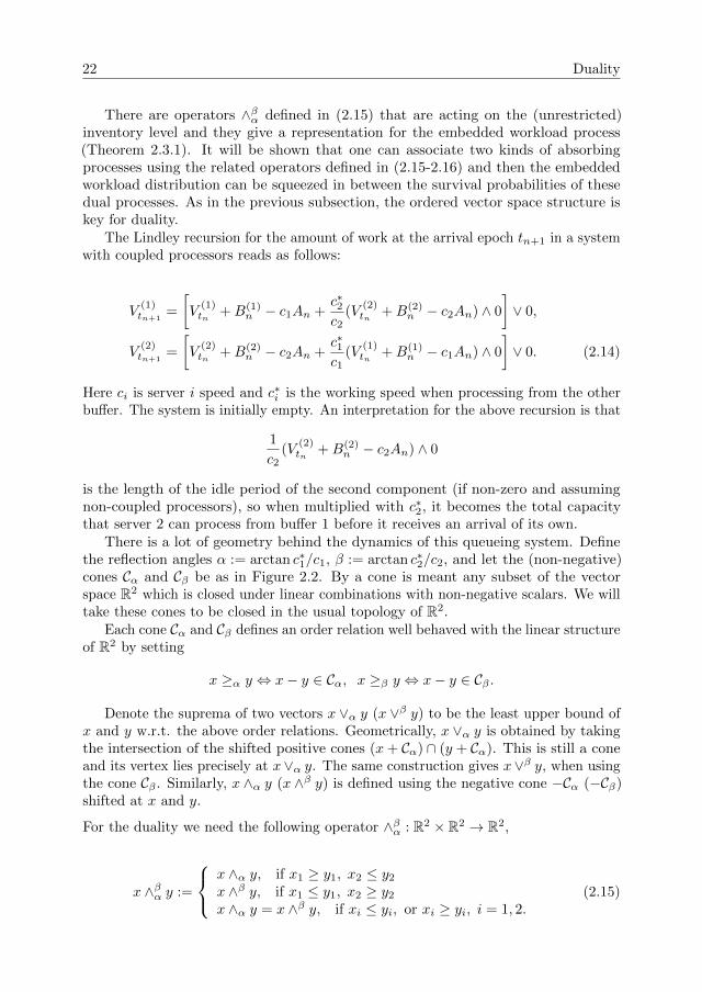
The Lindley recursion for the amount of work at the arrival epoch tn+1 in a systemwith coupled processors reads as follows:

V(1)tn+1

=

[V

(1)tn +B(1)

n − c1An +c∗2c2

(V(2)tn +B(2)

n − c2An) ∧ 0

]∨ 0,

V(2)tn+1

=

[V

(2)tn +B(2)

n − c2An +c∗1c1

(V(1)tn +B(1)

n − c1An) ∧ 0

]∨ 0. (2.14)

Here ci is server i speed and c∗i is the working speed when processing from the otherbuffer. The system is initially empty. An interpretation for the above recursion is that

1

c2(V

(2)tn +B(2)

n − c2An) ∧ 0

is the length of the idle period of the second component (if non-zero and assumingnon-coupled processors), so when multiplied with c∗2, it becomes the total capacitythat server 2 can process from buffer 1 before it receives an arrival of its own.

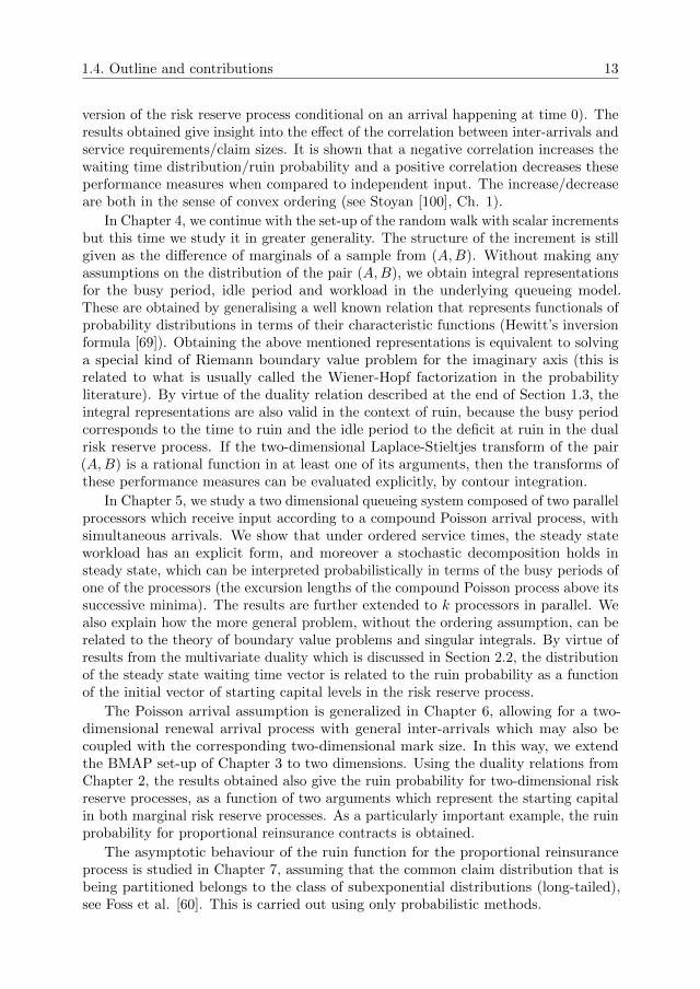
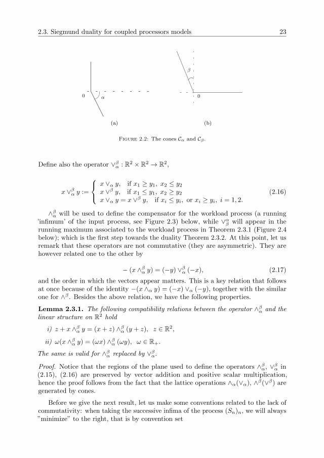
There is a lot of geometry behind the dynamics of this queueing system. Definethe reflection angles α := arctan c∗1/c1, β := arctan c∗2/c2, and let the (non-negative)cones Cα and Cβ be as in Figure 2.2. By a cone is meant any subset of the vectorspace R2 which is closed under linear combinations with non-negative scalars. We willtake these cones to be closed in the usual topology of R2.

Each cone Cα and Cβ defines an order relation well behaved with the linear structureof R2 by setting

x ≥α y ⇔ x− y ∈ Cα, x ≥β y ⇔ x− y ∈ Cβ .

Denote the suprema of two vectors x ∨α y (x ∨β y) to be the least upper bound ofx and y w.r.t. the above order relations. Geometrically, x ∨α y is obtained by takingthe intersection of the shifted positive cones (x+ Cα) ∩ (y + Cα). This is still a coneand its vertex lies precisely at x∨α y. The same construction gives x∨β y, when usingthe cone Cβ . Similarly, x ∧α y (x ∧β y) is defined using the negative cone −Cα (−Cβ)shifted at x and y.

For the duality we need the following operator ∧βα : R2 × R2 → R2,

x ∧βα y :=

x ∧α y, if x1 ≥ y1, x2 ≤ y2

x ∧β y, if x1 ≤ y1, x2 ≥ y2

x ∧α y = x ∧β y, if xi ≤ yi, or xi ≥ yi, i = 1, 2.(2.15)

2.3. Siegmund duality for coupled processors models 23

α0

1

(a)

β

0

1

(b)

Figure 2.2: The cones Cα and Cβ .

Define also the operator ∨βα : R2 × R2 → R2,

x ∨βα y :=

x ∨α y, if x1 ≥ y1, x2 ≤ y2

x ∨β y, if x1 ≤ y1, x2 ≥ y2

x ∨α y = x ∨β y, if xi ≤ yi, or xi ≥ yi, i = 1, 2.(2.16)

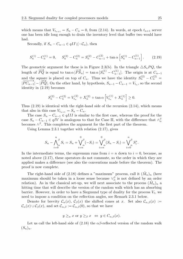
∧βα will be used to define the compensator for the workload process (a running’infimum’ of the input process, see Figure 2.3) below, while ∨αβ will appear in therunning maximum associated to the workload process in Theorem 2.3.1 (Figure 2.4below); which is the first step towards the duality Theorem 2.3.2. At this point, let usremark that these operators are not commutative (they are asymmetric). They arehowever related one to the other by

− (x ∧βα y) = (−y) ∨βα (−x), (2.17)

and the order in which the vectors appear matters. This is a key relation that followsat once because of the identity −(x ∧α y) = (−x) ∨α (−y), together with the similarone for ∧β . Besides the above relation, we have the following properties.

Lemma 2.3.1. The following compatibility relations between the operator ∧βα and thelinear structure on R2 hold

i) z + x ∧βα y = (x+ z) ∧βα (y + z), z ∈ R2,

ii) ω(x ∧βα y) = (ωx) ∧βα (ωy), ω ∈ R+.

The same is valid for ∧βα replaced by ∨βα.

Proof. Notice that the regions of the plane used to define the operators ∧βα, ∨βα in(2.15), (2.16) are preserved by vector addition and positive scalar multiplication,hence the proof follows from the fact that the lattice operations ∧α(∨α), ∧β(∨β) aregenerated by cones.

Before we give the next result, let us make some conventions related to the lack ofcommutativity: when taking the successive infima of the process (Sn)n, we will always”minimize” to the right, that is by convention set

24 Duality

x1 ∧βα x2 ∧βα x3 := (x1 ∧βα x2) ∧βα x3,

and we will ”maximize” to the left:

x1 ∨βα x2 ∨βα x3 := x1 ∨βα (x2 ∨βα x3).

These are successively defined for n vectors by iteration, and these conventions areconsistent with (2.17). This convention extends to n vectors when taking theirsuccessive infima and suprema, as in (2.18) below.

As usual, let Sn =∑nk=1Xk, X

(i)k := B

(i)k − ciAk, i = 1, 2, together with the

backwards coupled walk S∗k . The reason for introducing the above operators is thefollowing

Theorem 2.3.1. The solution to the Lindley recursion (2.14) can be represented as

Vtn+1= Sn −

n∧β

αi=0

Si.

Moreover, the compatibility between order and vector space structure implies thefollowing relation:

Sn −n∧β

αi=0

Si =

n∨β

αi=0

S∗i . (2.18)

Proof. The first part of the proof is similar to the proof of Proposition 2.2.1. Let usdenote the quadrants of the plane with qI − qIV . The positive quadrant is qI and therest are defined based on the trigonometric order. Proceeding by induction, (2.3.1)holds trivially for Vt1 . Assume the identity to be valid for Vtn . If we denote by

Cn−1 :=

n−1∧β

αi=0

Si,

then the following cases will be considered, depending on the position of Sn relativeto Cn−1.

Case I: Sn − Cn−1 ∈ qI, and then, by definition, ∧βα ≡ ∧α ≡ ∧β , so that Cn =Cn−1∧βαSn = Cn−1. Using the induction hypothesis, we can write Sn−Cn = Vtn +Xn,this vector belonging to the first quadrant, so that it is equal to Vtn+1

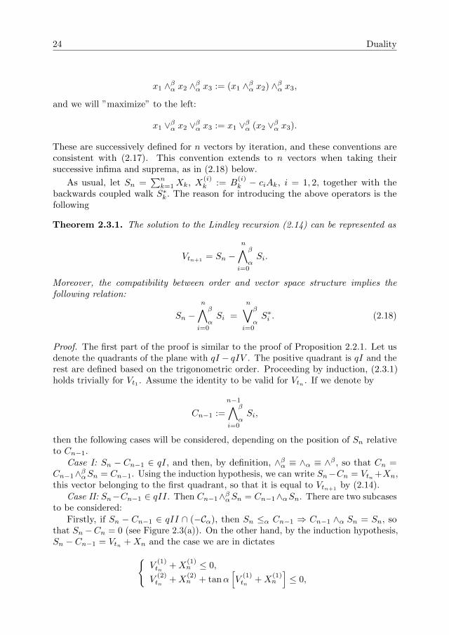
by (2.14).Case II: Sn−Cn−1 ∈ qII. Then Cn−1∧βαSn = Cn−1∧αSn. There are two subcases

to be considered:Firstly, if Sn − Cn−1 ∈ qII ∩ (−Cα), then Sn ≤α Cn−1 ⇒ Cn−1 ∧α Sn = Sn, so

that Sn −Cn = 0 (see Figure 2.3(a)). On the other hand, by the induction hypothesis,Sn − Cn−1 = Vtn +Xn and the case we are in dictates{

V(1)tn +X

(1)n ≤ 0,

V(2)tn +X

(2)n + tanα

[V

(1)tn +X

(1)n

]≤ 0,

2.3. Siegmund duality for coupled processors models 25

which means that Vtn+1= Sn − Cn = 0, from (2.14). In words, at epoch tn+1 server

one has been idle long enough to drain the inventory level that buffer two would havehad.

Secondly, if Sn − Cn−1 ∈ qII\(−Cα), then

S(1)n − C(1)

n = 0, S(2)n − C(2)

n = S(2)n − C(2)

n−1 + tanα[S(1)n − C(1)

n−1

]. (2.19)

The geometric argument for these is in Figure 2.3(b). In the triangle 4SnPQ, the

length of−−→PQ is equal to tanα |−→PSn| = tanα [S

(1)n − C(1)

n−1]. The origin is at Cn−1

and the square is placed on top of Cn. Thus we have the identity S(2)n − C(2)

n =

|−−−−→PCn−1| − |−−→PQ|. On the other hand, by hypothesis, Sn−1−Cn−1 = Vtn , so the second

identity in (2.19) becomes

S(2)n − C(2)

n = V(2)tn +X(2)

n + tanα[V

(1)tn +X(1)

n

]≥ 0.

Thus (2.19) is identical with the right-hand side of the recursion (2.14), which meansthat also in this case Vtn+1

= Sn − Cn.The case Sn − Cn−1 ∈ qIII is similar to the first case, whereas the proof for the

case Sn − Cn−1 ∈ qIV is analogous to that for Case II, with the difference that ∧βαbecomes ∧β . This completes the argument for the first part of the theorem.

Using Lemma 2.3.1 together with relation (2.17), gives

Sn −n∧β

αi=0

Si = Sn +

0∨β

αi=n

(−Si) =

0∨β

αi=n

(Sn − Si) =

n∨β

αi=0

S∗i .

In the intermediate terms, the supremum runs from i = n down to i = 0, because, asnoted above (2.17), these operators do not commute, so the order in which they areapplied makes a difference (see also the conventions made before the theorem). Theproof is now complete.

The right-hand side of (2.18) defines a ”maximum” process, call it (Mn)n (heremaximum should be taken in a loose sense because ∨βα is not defined by an orderrelation). As in the classical set-up, we will next associate to the process (Mn)n ahitting time that will describe the version of the random walk which has an absorbingbarrier. However, in order to have a Siegmund type of duality for the process Vt, weneed to impose a condition on the reflection angles, see Remark 2.3.1 below.

Denote for brevity Cα(x), Cβ(x) the shifted cones at x. Set also Cα,β(x) :=Cα(x) ∪ Cβ(x), and set Cα,β := Cα,β(0), so that we have

y ≥α x or y ≥β x ⇔ y ∈ Cα,β(x).

Let us call the left-hand side of (2.18) the αβ-reflected version of the random walk(Sn)n.

26 Duality

α

Cn−1

Sn

1

(a)

α

Cn−1

CnQ

P

Sn

1

(b)

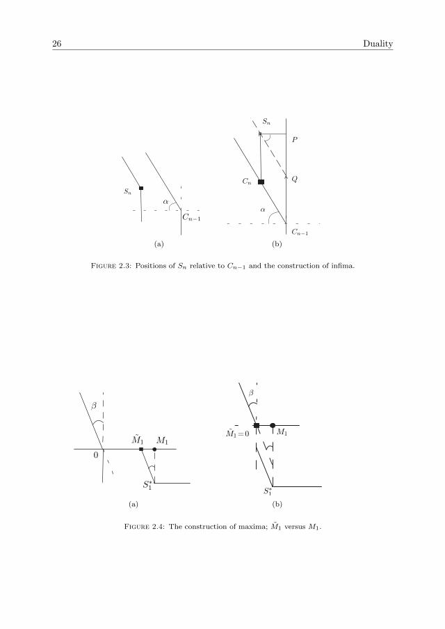
Figure 2.3: Positions of Sn relative to Cn−1 and the construction of infima.

β

0

M1 M1

S∗1

1

(a)

β

M1=0 M1

S∗1

1

(b)

Figure 2.4: The construction of maxima; M1 versus M1.

2.3. Siegmund duality for coupled processors models 27

Remark 2.3.1. The possibility to have an identity between the law of the αβ-reflectedprocess (Vtn)n and a process with an absorbing domain relies on the validity of thefollowing equivalence (see also (2.18))

x ∨βα y ∈ −Cα,β ⇔ x, y ∈ −Cα,β ,for arbitrary vectors x, y ∈ R2. In words, knowing that the running ∨α,β-supremumbelongs to some subset of R2, we must be able to infer on the position of each componentthat appears in the supremum. In contrast to the set-up of Section 2.2, where we canfind such an equivalence for the negative cones, see for example (2.12), in the presentset-up this is not always possible anymore. It is easy to see that this equivalence holdsonly when α+ β = π/2 (α > 0 or β > 0, otherwise, if α = β = 0 the equivalence holds,but we are back in the instance from Subsection 2.2).In more generality, let Ccα,β(u) be the topological closure of the complementary ofCα,β(u).

If α+ β ≤ π/2, then Ccα,β(u) ⊇ −Cα,β(u), and the following chain of implicationsis valid

x ∨βα y ∈ −Cα,β(u)⇒ x, y ∈ −Cα,β(u)⇒ x ∨βα y ∈ Ccα,β(u)⇒ x, y ∈ Ccα,β(u).

If α + β ≥ π/2, then Ccα,β(u) ⊆ −Cα,β(u) and the converse chain holds. Thesecan be argued directly from definition (2.16), by considering all the cases, based on theposition of y relative to x, just like in the proof of Theorem 2.3.1.

Consider (Sa

n)n, the version of the random walk u − S∗n =: Rt∗n+1, killed upon

exiting −Ccα,β , and (San)n, the version killed upon exiting Cα,β .

Theorem 2.3.2 (Siegmund Duality). There exists a duality relation between the αβ-reflected version (Vtn)n of (Sn)n, conditional on Vt1 = x and the laws of the absorbedrandom walks (San)n and (S

a

n)n. More precisely, under the condition α+ β ≤ π/2, itholds for x ≥ 0, n ≥ 1 that

P(Vtn ∈ −Cα,β(u)|Vt1 = x) ≤ P(San ∈ Cα,β(x)|Sa0 = u) ≤P(Vtn ∈ Ccα,β(u)|Vt1 = x) ≤ P(S

a

n ∈ −Ccα,β(x)|Sa1 = u), u ∈ Cα,β , (2.20)

and if α+β ≥ π/2, the chain of inequalities is reversed and valid whenever u ∈ −Ccα,β(see Remark 2.3.1).

In particular, if α+ β = π/2, the αβ-reflected version of the random walk has thesame law as the version (San)n ≡ (S

a

n)n, absorbed upon exiting Cα,β ≡ −Ccα,β, (cf.(2.13)):

P(Vtn ∈ −Cα,β(u)|Vt1 = x) = P(San ∈ Cα,β(x)|Sa0 = u), u ∈ Cα,β . (2.21)

Notice that the event on the right-hand side of (2.21) implies San has not beenkilled up to epoch t∗n, that is we have

28 Duality

P(San ∈ Cα,β(x)|Sa0 = u) = P(Sak ∈ Cα,β , k ≤ n− 1, San ∈ Cα,β(x)|Sa0 = u). (2.22)

Proof of Theorem 2.3.2. The proof is a variation of Theorem 2.3.1. The extra featureis that the solution of the Lindley recursion was given under the condition Vt1 = 0,and now we adapt it to the case Vt1 = x. Making use of the operators introduced, webegin with the remark that recursion (2.14) can be represented as (mind the order inwhich the supremum is taken)

Vtn+1= 0 ∨βα (Vtn +Xn+1).

Iterating this recursion via Lemma 2.3.1 with initial condition Vt1 = x, gives alongthe same lines as in the proof of Theorem 2.3.1:

Vtn+1= 0 ∨βα S∗1 ∨βα S∗2 ∨βα . . . ∨βα (S∗n + x), (2.23)

where Vt1 = x appears in the rightmost term only.Under the condition α+ β ≤ π/2, the chain of inequalities from Remark 2.3.1 is in

force, and thus we can write using (2.23), for an arbitrary u ∈ Cα,β :

Vtn+1∈ −Cα,β(u)⇒ S∗k ∈ −Cα,β(u), k ≤ n− 1, S∗n + x ∈ −Cα,β(u),

which is the same as San ∈ Cα,β(x), via (2.22). Finally, (2.20) follows similarly fromthe rest of the chain of inequalities from Remark 2.3.1.

The case α+ β ≥ π/2 follows from the second part of Remark 2.3.1, because inthis case we have the converse implications. This completes the proof.

Concluding remarks

Ergodicity. Focus first on the case α+ β ≤ π/2. For the embedded random walk(u− S∗n)n starting at u ∈ Cα,β , define its first exit time from Cα,β :

τα,β(u) = min{t∗n; S∗n ≯α u, and S∗n ≯β u}.The second inequality from (2.20) becomes via (2.22), for x = 0, u ∈ Cα,β :

P(Vtn ∈ Ccα,β(u)|Vt1 = 0) ≥ P(Sak ∈ Cα,β , k ≤ n|Sa0 = u) = P(τα,β(u) > t∗n), (2.24)

(cf. (2.13)). Since (Vtn)n is a regenerative process with 0 as regeneration point, Vtnconverges weakly as n→∞ to a proper probability distribution Vt∞ , whenever it has0 as a positive recurrent state, and then by (2.24), the hitting time τα,β(0) must havepositive probability of never occurring, i.e., (2.24) with u = 0 must read in the limit

P(Vt∞ = 0) ≥ P(τα,β(0) =∞) > 0.

2.3. Siegmund duality for coupled processors models 29

Thus, a sufficient condition that ensures ergodicity for (Vtn)n is that the mean incrementE(−X1) of San must lie in the topological interior C◦α,β . In words, (San)n must driftaway from its absorbing domain.

That the necessary condition is E(−X1) ∈ Cα,β , follows along the same lines byusing the first inequality from (2.20) (which gives the upper bound on the distributionfunction of Vt∞).

For the case α+ β ≥ π/2, the discussion is analogous. One has to redefine τα,β to

be the exit time of Sa

n from the (closed, convex) set −Ccα,β . The chain of inequalitiesin (2.20) is reversed so one should use the last inequality that reads in the currentcase:

P(Vtn ∈ Ccα,β(u)|Vt1 = x) ≥ P(Sa

n ∈ −Ccα,β(x)|Sa1 = u),

for u ∈ Ccα,β . The same arguments as in the previous case give that the mean drift

E(−X1) of Sa

n must belong to −Ccα,β , and in the current case, this is sufficient toensure the queueing system is stable. Remark that in both cases, the domain insidewhich the random walk is allowed to evolve before absorbtion is closed and convex.

In Cohen and Boxma [41], the study of the amount of work in the coupled processormodel is reduced to a functional equation in terms of Laplace-Stieltjes transforms, whichis then further related to a boundary value problem of Riemann type. They assumeindependent Poisson arrivals with intensities λi and independent service requirementsbetween the queues. In our case, the arrival streams are merged with common arrivalintensity, say, λ ( λ = λ1 + λ2, hence service requirements are correlated among thequeues, and since a type 1 arrival will demand no work from queue 2, the traffic loadsremain the same). Synchronizing notations - the model description is different, butequivalent, see [41, p. 288, pp. 294-296] - they have

ρ1 := 1 +c∗2c1≥ 1, ρ2 := 1 +

c∗1c2≥ 1,

and further, the natural server rates are normalized to c2 = c1 = 1, so that thereflection angles in our notation become tanα = ρ2 − 1, tanβ = ρ1 − 1 (the ρi’s in[41] have a different meaning than the usual load coefficients). It is easy to see thatthe ergodicity condition extracted in [41] from the study of the functional equationreads in our notation

b1 := λEB(1)

(1− 1

1 + c∗1

)+λEB(2)

1 + c∗1< 1, b2 :=

λEB(1)

1 + c∗2+λEB(2)

(1− 1

1 + c∗2

)< 1,

and is equivalent to the conditions

EX(2)1 + tanαEX(1)

1 < 0, EX(1)1 + tanβ EX(2)

1 < 0, (2.25)

which in case α + β ≤ π/2 is the same as E(−X1) ∈ C◦α,β , and it is equivalent toE(−X1) ∈ Ccα,β for α+ β ≥ π/2. In any case, (2.25) means the mean drift vector mustpoint into the interior of the intersection of the lower hyperplanes at 0 with directionvectors (tanα, 1) and respectively (1, tanβ).

30 Duality

In conclusion, the stability condition for the coupled processor model studied inCohen and Boxma [41] is the same as the ergodicity condition for the dual absorbedprocess San, as predicted by the duality relation (2.20). The result of Theorem 2.3.2 isvalid under very general assumptions on the arrival process; for example, a semi-Markovstructure for the arrival process preserves this ergodicity condition.

Large deviations. The possibility to infer on the positions of the walks San and Sa

n

based on the position of the all-time maximum M∞ is the usual method for analyzingoverflow probabilities, either when increments are light-tailed or heavy-tailed. Assumefor simplicity α+ β = π/2, then under the stability condition (2.25), (2.20) becomesin the limit

P(Vt∞ /∈ −Cα,β(u)) = P(∃n0; San0/∈ Cα,β |Sa0 = u),

and the right-hand side is typically the starting point for the study of large deviations.

Simulation. One of the reasons why Siegmund [97] studied such duality relationsis that estimating the hitting probabilities for the absorbed process is more efficientnumerically than the problem of estimating the equilibrium distribution for thedual reflecting process (this is the usual Markov-Chain-Monte-Carlo scheme, theefficiency of which depends severely on the mixing properties of the chain). Forα + β = π/2, Theorem 2.3.2 gives a numerical scheme for simulating exactly theequilibrium distribution of the embedded workload in the system, and it providesbounds otherwise.

Chapter 3

Single server queues andSparre-Andersen risk reserveprocesses with correlations

This chapter deals with the study of performance measures related to single serverqueues and their dual Sparre-Andersen risk reserve processes which have a form ofdependence between inter-arrival times and service requirements/claim sizes. Thesemodels were introduced and described in Section 1.1. The main contributions of thecurrent chapter are the following: (i) We provide an exact analysis of the waiting timedistribution in a GI/G/1 queue with correlation between a service requirement B andthe subsequent inter-arrival time A, B and A having a multivariate matrix-exponentialdistribution. Via (2.6), the distribution of the waiting time is then immediately relatedto the ruin probability of the dual risk reserve process. (ii) We prove that the simplerelation which holds between steady-state workload and waiting time distributionsin the ordinary GI/GI/1 queue remains valid in the case of correlated B and A.(iii) We consider the dual Sparre-Andersen insurance risk model with correlationbetween inter-claim time and subsequent claim size, and in particular we show thatthe Takacs relation (cf. [63], Corollary 4.5.4) between the ordinary ruin probabilityand the delayed ruin probability remains valid; and this is analogous to the relationbetween the steady-state waiting time and the workload. (iv) Finally, we show that,in comparison with the classical set-up with mutually independent sequences (Ak)k≥1

and (Bk)k≥1, positive and negative correlation respectively decreases and increasesthe waiting times in the sense of convex ordering. We also illustrate with numericalresults the influence of dependence on the expected values of the waiting times butalso on the 95%-percentiles of the ruin functions (values at risk) - the quantiles of theruin function correspond to the values of the waiting time tail, again via (2.6).

The chapter is organized as follows. Section 3.1 contains a detailed model descrip-tion, which in particular includes a description of the class of bivariate distributionsunder consideration. It also presents the waiting time analysis. The relation betweenthe steady-state waiting time and workload distributions is exposed in Section 3.2.

31

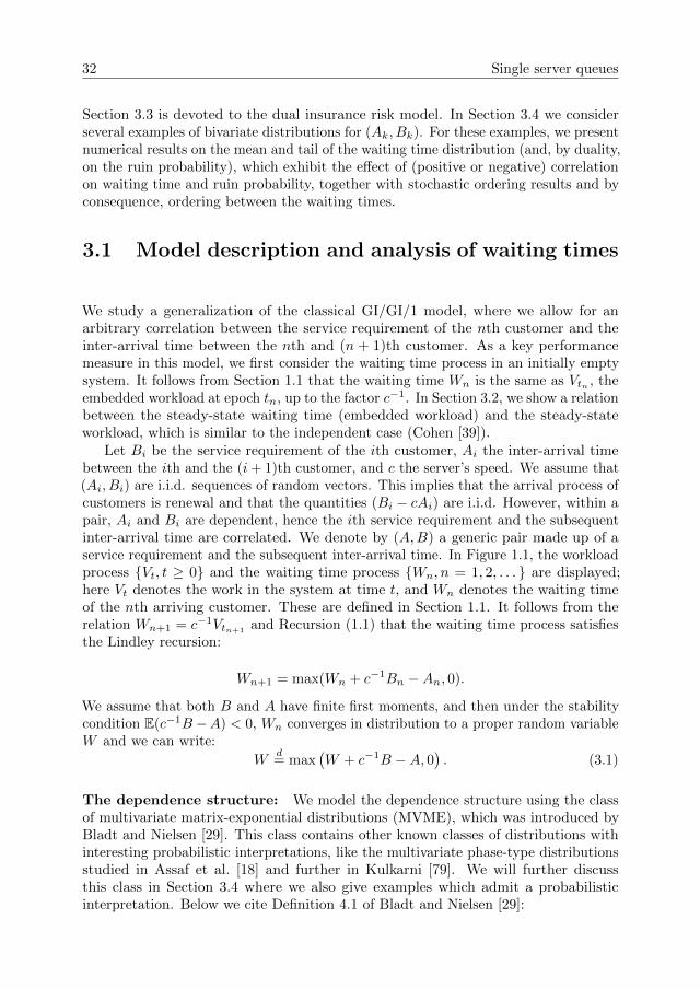
32 Single server queues

Section 3.3 is devoted to the dual insurance risk model. In Section 3.4 we considerseveral examples of bivariate distributions for (Ak, Bk). For these examples, we presentnumerical results on the mean and tail of the waiting time distribution (and, by duality,on the ruin probability), which exhibit the effect of (positive or negative) correlationon waiting time and ruin probability, together with stochastic ordering results and byconsequence, ordering between the waiting times.

3.1 Model description and analysis of waiting times

We study a generalization of the classical GI/GI/1 model, where we allow for anarbitrary correlation between the service requirement of the nth customer and theinter-arrival time between the nth and (n + 1)th customer. As a key performancemeasure in this model, we first consider the waiting time process in an initially emptysystem. It follows from Section 1.1 that the waiting time Wn is the same as Vtn , theembedded workload at epoch tn, up to the factor c−1. In Section 3.2, we show a relationbetween the steady-state waiting time (embedded workload) and the steady-stateworkload, which is similar to the independent case (Cohen [39]).

Let Bi be the service requirement of the ith customer, Ai the inter-arrival timebetween the ith and the (i+ 1)th customer, and c the server’s speed. We assume that(Ai, Bi) are i.i.d. sequences of random vectors. This implies that the arrival process ofcustomers is renewal and that the quantities (Bi − cAi) are i.i.d. However, within apair, Ai and Bi are dependent, hence the ith service requirement and the subsequentinter-arrival time are correlated. We denote by (A,B) a generic pair made up of aservice requirement and the subsequent inter-arrival time. In Figure 1.1, the workloadprocess {Vt, t ≥ 0} and the waiting time process {Wn, n = 1, 2, . . . } are displayed;here Vt denotes the work in the system at time t, and Wn denotes the waiting timeof the nth arriving customer. These are defined in Section 1.1. It follows from therelation Wn+1 = c−1Vtn+1

and Recursion (1.1) that the waiting time process satisfiesthe Lindley recursion:

Wn+1 = max(Wn + c−1Bn −An, 0).

We assume that both B and A have finite first moments, and then under the stabilitycondition E(c−1B−A) < 0, Wn converges in distribution to a proper random variableW and we can write:

Wd= max

(W + c−1B −A, 0

). (3.1)

The dependence structure: We model the dependence structure using the classof multivariate matrix-exponential distributions (MVME), which was introduced byBladt and Nielsen [29]. This class contains other known classes of distributions withinteresting probabilistic interpretations, like the multivariate phase-type distributionsstudied in Assaf et al. [18] and further in Kulkarni [79]. We will further discussthis class in Section 3.4 where we also give examples which admit a probabilisticinterpretation. Below we cite Definition 4.1 of Bladt and Nielsen [29]:

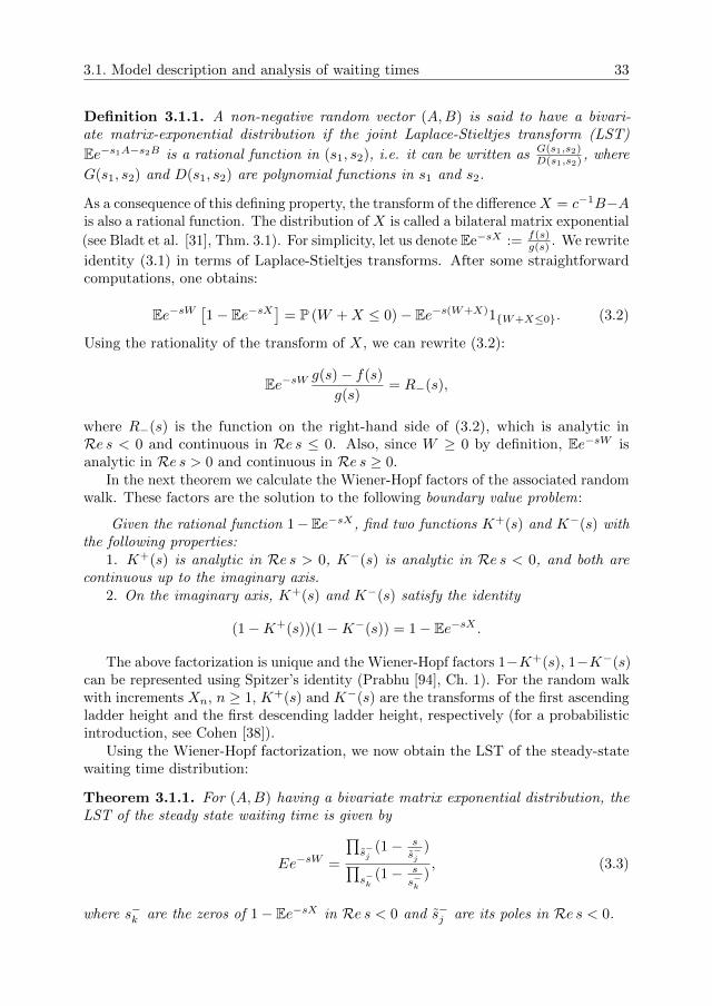
3.1. Model description and analysis of waiting times 33

Definition 3.1.1. A non-negative random vector (A,B) is said to have a bivari-ate matrix-exponential distribution if the joint Laplace-Stieltjes transform (LST)

Ee−s1A−s2B is a rational function in (s1, s2), i.e. it can be written as G(s1,s2)D(s1,s2) , where

G(s1, s2) and D(s1, s2) are polynomial functions in s1 and s2.

As a consequence of this defining property, the transform of the differenceX = c−1B−Ais also a rational function. The distribution of X is called a bilateral matrix exponential

(see Bladt et al. [31], Thm. 3.1). For simplicity, let us denote Ee−sX := f(s)g(s) . We rewrite

identity (3.1) in terms of Laplace-Stieltjes transforms. After some straightforwardcomputations, one obtains:

Ee−sW[1− Ee−sX

]= P (W +X ≤ 0)− Ee−s(W+X)1{W+X≤0}. (3.2)

Using the rationality of the transform of X, we can rewrite (3.2):

Ee−sWg(s)− f(s)

g(s)= R−(s),

where R−(s) is the function on the right-hand side of (3.2), which is analytic inRe s < 0 and continuous in Re s ≤ 0. Also, since W ≥ 0 by definition, Ee−sW isanalytic in Re s > 0 and continuous in Re s ≥ 0.

In the next theorem we calculate the Wiener-Hopf factors of the associated randomwalk. These factors are the solution to the following boundary value problem:

Given the rational function 1−Ee−sX , find two functions K+(s) and K−(s) withthe following properties:

1. K+(s) is analytic in Re s > 0, K−(s) is analytic in Re s < 0, and both arecontinuous up to the imaginary axis.

2. On the imaginary axis, K+(s) and K−(s) satisfy the identity

(1−K+(s))(1−K−(s)) = 1− Ee−sX .

The above factorization is unique and the Wiener-Hopf factors 1−K+(s), 1−K−(s)can be represented using Spitzer’s identity (Prabhu [94], Ch. 1). For the random walkwith increments Xn, n ≥ 1, K+(s) and K−(s) are the transforms of the first ascendingladder height and the first descending ladder height, respectively (for a probabilisticintroduction, see Cohen [38]).

Using the Wiener-Hopf factorization, we now obtain the LST of the steady-statewaiting time distribution:

Theorem 3.1.1. For (A,B) having a bivariate matrix exponential distribution, theLST of the steady state waiting time is given by

Ee−sW =

∏s−j

(1− ss−j

)∏s−k

(1− ss−k

), (3.3)

where s−k are the zeros of 1− Ee−sX in Re s < 0 and s−j are its poles in Re s < 0.

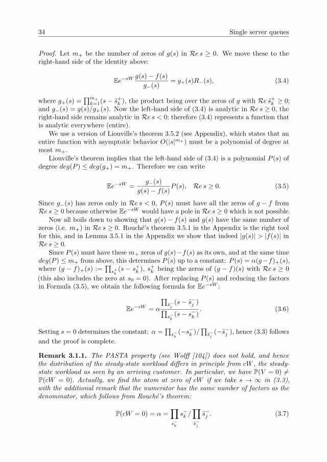
34 Single server queues

Proof. Let m+ be the number of zeros of g(s) in Re s ≥ 0. We move these to theright-hand side of the identity above:

Ee−sWg(s)− f(s)

g−(s)= g+(s)R−(s), (3.4)

where g+(s) =∏m+

k=1(s− s+k ), the product being over the zeros of g with Re s+

k ≥ 0;and g−(s) = g(s)/g+(s). Now the left-hand side of (3.4) is analytic in Re s ≥ 0, theright-hand side remains analytic in Re s < 0; therefore (3.4) represents a function thatis analytic everywhere (entire).

We use a version of Liouville’s theorem 3.5.2 (see Appendix), which states that anentire function with asymptotic behavior O(|s|m+) must be a polynomial of degree atmost m+.

Liouville’s theorem implies that the left-hand side of (3.4) is a polynomial P (s) ofdegree deg(P ) ≤ deg(g+) = m+. Therefore we can write

Ee−sW =g−(s)

g(s)− f(s)P (s), Re s ≥ 0. (3.5)

Since g−(s) has zeros only in Re s < 0, P (s) must have all the zeros of g − f fromRe s ≥ 0 because otherwise Ee−sW would have a pole in Re s ≥ 0 which is not possible.

Now all boils down to showing that g(s)− f(s) and g(s) have the same number ofzeros (i.e. m+) in Re s ≥ 0. Rouche’s theorem 3.5.1 in the Appendix is the right toolfor this, and in Lemma 3.5.1 in the Appendix we show that indeed |g(s)| > |f(s)| inRe s ≥ 0.

Since P (s) must have these m+ zeros of g(s)−f(s) as its own, and at the same timedeg(P ) ≤ m+ from above, this determines P (s) up to a constant: P (s) = α(g−f)+(s),where (g − f)+(s) :=

∏s+k

(s − s+k ), s+

k being the zeros of (g − f)(s) with Re s ≥ 0

(this also includes the zero at s0 = 0). After replacing P (s) and reducing the factorsin Formula (3.5), we obtain the following formula for Ee−sW :

Ee−sW = α

∏s−j

(s− s−j )∏s−k

(s− s−k ). (3.6)

Setting s = 0 determines the constant: α =∏s−k

(−s−k )/∏s−j

(−s−j ), hence (3.3) follows

and the proof is complete.

Remark 3.1.1. The PASTA property (see Wolff [104]) does not hold, and hencethe distribution of the steady-state workload differs in principle from cW , the steady-state workload as seen by an arriving customer. In particular, we have P(V = 0) 6=P(cW = 0). Actually, we find the atom at zero of cW if we take s → ∞ in (3.3),with the additional remark that the numerator has the same number of factors as thedenominator, which follows from Rouche’s theorem:

P(cW = 0) = α =∏s−k

s−k /∏s−j

s−j . (3.7)

3.1. Model description and analysis of waiting times 35

On the other hand, from first principles we have, with ρ := EBcEA , for the steady-state

probability of an empty system:

P(V = 0) = 1− ρ.

The factorization used in the proof of identity (3.3) can be also used to obtain thetransform EesI of I, the steady state idle period of the system.

Corollary 3.1.1. The transform of the idle period is given by

EesI = 1−∏s+k

(s− s+k )/

∏s+j

(s− s+j ), Re s ≤ 0,

with s+k being the zeroes of g(s)−f(s)

g(s) in Re s ≥ 0 and s+j its poles in Re s > 0.

Proof. Conditional on W +X ≤ 0, I = −(W +X), so we may write

EesI =1

P(W +X ≤ 0)Ees(−W−X)1{W+X≤0}, Re s ≤ 0.

The transform Ees(−W−X)1{W+X≤0} already appears on the right-hand side of (3.2),hence the transform of the idle period can be rewritten as

EesI = 1− 1

P(W +X ≤ 0)· Ee−sW · g(s)− f(s)

g(s). (3.8)

As in the proof of Theorem 3.1.1, we make use of the factorizations g(s) =g+(s) · g−(s) and (g − f)(s) = (g − f)+(s) · (g − f)−(s) which were obtained viaRouche’s theorem. Therefore, using (3.5), (3.6) and (3.7) we may write

EesI = 1− P(W = 0)

P(W +X ≤ 0)· g−(s)

(g − f)−(s)· g(s)− f(s)

g(s).

Note that the identity in law (3.1) implies P(W = 0) = P(W+X ≤ 0). After cancellingthe factors above, EesI reduces to

EesI = 1−∏s+k

(s− s+k )/

∏s+j

(s− s+j ).

Remark 3.1.2. Alternatively we can use Formula (6.20) in Cohen [39], p. 21, whichmakes use of the regenerative structure of the workload process w.r.t. the busy cycles ofthe queue. It can be shown that the formula remains valid even in the dependent case.The connection with (3.8) is then 1

P(W+X≤0) = EN , the mean number of customers

served during a busy cycle.

In the next section we show that similar arguments involving regeneration as theones employed in [39], can be extended in our setting to give the relation between thesteady-state workload and waiting time distributions.

36 Single server queues

3.2 The steady-state workload

In this section we consider the steady-state workload in the queueing model withcorrelation between service requirement B and subsequent inter-arrival time A. Weshall prove that the known relation between the steady-state workload and waitingtime for the single server queue with independent service requirement and inter-arrivaltime (Asmussen [16], p. 274, Cohen [39], p. 19-20, or [40], p. 296, 297) remainsvalid. For this purpose we adapt the proof in [39], which is based on the fact thatthe workload process regenerates at the beginning of each busy cycle. The LST ofthe workload and waiting time distributions can then be written as stochastic meanvalues of the LST over one full busy cycle.

Theorem 3.2.1. The steady-state workload V and the waiting time W are related inthe following way:

P(V ≤ v) = 1− ρ+ ρP(cW +Bres ≤ v), (3.9)

with ρ = EBcEA and Bres the marginal distribution of a residual service requirement, viz.,

P(Bres ≤ v) = 1EB

v∫0

P(B > u) du.

Remark that only the marginal distribution of the residual service requirementappears in the above, not the joint distribution of A and B.

Proof. Let 0 be the beginning of a busy period and P be its length. Following Cohen[39], within this busy period, we may write (cf. Figure 1.1):

Vt = cWn(t) +Bn(t) − c(t− tn(t)),

where Vt is the workload at time t, n(t) is the number of arrivals in [0, t] and tn(t) isthe last arrival epoch before t. The following identities hold path-wise:∫ P

0

e−sVtdt =

∫ P

0

e−s[cWn(t)+Bn(t)−c(t−tn(t))] dt

=N−1∑i=1

∫ Ai

0

e−s(cWi+Bi−ct)dt+

∫ AN−I

0

e−s(cWN+BN−ct) dt. (3.10)

Here N is the number of customers served during a busy period. The key observationis that the following relation holds even when Ai and Bi are dependent:∫ Ai

0

e−s(cWi+Bi−ct)dt = e−s(cWi+Bi)1

cs(ecsAi − 1).

There is no expectation taken so integration is carried out as usual, all these beingpath-wise identities. Formula (3.10) now becomes

3.2. The steady-state workload 37

P∫0

e−sVt dt =1

cs

N−1∑i=1

e−s(cWi+Bi)[ecsAi − 1

]+

1

cse−s(cWN+BN )

[ecs(AN−I) − 1

]

=1

cs

N−1∑i=1

[e−s(cWi+Bi−cAi) −e−s(cWi+Bi)

]+

1

cse−s[cWN+BN−c(AN−I)]

− 1

cse−s(cWN+BN ).

We make use of the following identities for the waiting time during a busy period:For i ≤ N − 1, cWi +Bi − cAi = cWi+1; and cWN +BN − cAN = −cI, hence

P∫0

e−sVt dt =1

cs

N−1∑i=1

(e−scWi+1 − e−scWi−sBi)+

1

cs

[1− e−scWN−sBN ]

=1

cs

N∑i=1

e−scWi(1− e−sBi). (3.11)

All derivations up to this point are path-wise manipulations, hence insensitive tocorrelations between Ai and Bi. Remark that Bn is independent of Wn but also ofthe r.v. 1{N≥n}. So if we take expectations in (3.11)

EP∫

0

e−sVt dt =1

csE∞∑n=1

[e−scWn1{N≥n}(1− e−sBn)

]= E

( ∞∑n=1

e−scWn1{N≥n}

)1− Ee−sB1

cs,

so that

EP∫

0

e−sVt dt = E

(N∑i=1

e−scWi

)1− Ee−sB1

cs. (3.12)

A key remark is that the workload process is still regenerative with respect to therenewal sequence given by the epochs at which busy periods begin. Under the stabilitycondition, the mean cycle length EC (C is the length of a regeneration cycle) of theworkload process is finite, hence the stochastic mean value results still hold in thiscase (cf. Cohen [39], Thm. 4.1) and we have the identities:

Ee−sV =1

ECE

C∫0

e−sVt dt,

38 Single server queues

and

Ee−sW =1

ENE

N∑1

e−sWi .

We can now use these identities together with (3.12) and EC = EP + EI, so we maywrite

Ee−sV =

EP∫0

e−sVt dt+ EI

EP + EI=EN EBEC

Ee−scW1− Ee−sBcsEB

+EIEC

.

Note that by definition, P =∑Ni=1 c

−1Bi, with (Bi)i the i.i.d. sequence such that Biis the service requirement of the ith customer in a busy cycle. Hence Wald’s identitygives cEP = EN EB, and using in addition EP

EC = ρ, EIEC = 1− ρ , we can rewrite the

above as

Ee−sV = ρ1− Ee−sBsEB

Ee−scW + (1− ρ), Re s ≥ 0.

This can immediately be inverted to give the desired relation (3.9), which concludesthe proof.

3.3 Duality between the insurance and queueingprocesses

It is well known that there are duality relations between the classical GI/GI/1 queue andthe corresponding classical Sparre-Andersen insurance risk model, with independencebetween service requirements (respectively claim sizes) and inter-arrival times. In thiscase ‘corresponding’ means: the same inter-arrival distributions, and that the servicerequirement distribution equals the claim size distribution, the service rate c is thesame as the premium rate. There are two versions of the duality result (cf. Asmussenand Albrecher [17], p. 45, 161):

(i) Ψ0(u) = P(cW > u), (3.13)

(ii) Ψ(u) = P(V > u). (3.14)

Here P(cW > u) is the tail of the amount of work as seen by an arriving customerin equilibrium, and P(V > u) is the tail of the steady-state workload in the G/G/1queue. Ψ0(u) is the ruin probability in the Sparre-Andersen model, when at timet = 0 the capital is u and a new inter-arrival time begins, i.e., t = 0 is an arrival epoch.Ψ(u) is the ruin probability when the risk process is started in stationarity, i.e., t = 0is independent of the process itself. In this case the time elapsed until the first claimarrives has a residual distribution. We will call Ψ0(u) the ordinary ruin probabilityand Ψ(u) the delayed ruin probability. It is also worth to notice that the relationsobtained in this section between Ψ0 and Ψ do not use the bilateral matrix exponentialstructure of the increments Xn.

3.3. Duality between the insurance and queueing processes 39

We pose and answer three questions in this section, for the dependencies underconsideration (between service requirement and subsequent inter-arrival time, respec-tively between inter-claim time and subsequent claim size):(1) Does the duality relation (3.13) still hold?(2) Does the duality relation (3.14) still hold?(3) Does the relation between steady-state workload and waiting time from Theo-rem 3.2.1 translate to a relation between delayed ruin probability and ordinary ruinprobability, just as it does in the independent case (cf. p. 69 of Grandell [68])?

The answer to question (1) is immediately seen to be positive, as shown in Asmussenand Albrecher [17] p. 45, because this relation uses only the random walk structure ofthe risk/queueing process embedded at arrival epochs, which is preserved in the modelwe study (Bi and Ai only appear in the random walk via the difference Bi − cAi).The Laplace transform of the ruin probability now immediately follows from thewaiting time LST in Theorem 3.1.1, by observing that the relation Ψ0(u) = P(cW > u)becomes in terms of transforms: Ψ∗0(s) = 1

s

(1− Ee−scW

). Hence we have:

Corollary 3.3.1. The Laplace transform of Ψ0(u), Ψ∗0(s) :=∫∞

0e−suΨ0(u) du equals

Ψ∗0(s) =1

s

1−∏s−j

(1− css−j

)∏s−k

(1− css−k

)

.This result was also obtained in Constantinescu et al. [48], using operator theory.We shall prove that the answer to question (3) is also affirmative. In combination

with the duality relation (3.13), this implies that the answer to question (2) is alsoaffirmative: the duality relation (3.14) still holds in the dependent case.

For the purpose of studying the relation between the ordinary and the delayedruin functions below, we assume that the pair (A,B) has a joint density, fA,B(r, z).Let φ0(u) := 1−Ψ0(u) and φ(u) := 1−Ψ(u) be the survival functions for the ordinaryrisk process and for its stationary version, respectively. In addition, denote by u theinitial capital, and let α := 1

EA be the arrival rate of claims.

Theorem 3.3.1. The relation between the survival functions for the two versions ofthe ruin process is

φ(u) = φ(0) +α

c

∞∫v=0

u∫w=0

φ0(u− w)

∞∫z=w

fA,B(v, z) dz dw dv.

Let us make some remarks about this formula before proving it.

Remark 3.3.1. In the stationary version of the ruin process, the first claim arrivalhappens after a time distributed as the residual inter-arrival time. Because of thecorrelation between claim sizes and their inter-arrival times, the claim size thatcorresponds to the residual arrival time will have a distinguished distribution; thereforelet us denote the first pair by (Ares, B∗). Regarding the density function, it can beshown that (see Lemma 3.5.3)

40 Single server queues

fAres,B∗(r, z) = α

∞∫v=r

fA,B(v, z) dv. (3.15)

Remark 3.3.2. The double integral that appears in the last term from Theorem 3.3.1above: ∞∫

v=0

∞∫z=w

fA,B(v, z) dz dv

equals the marginal tail of a claim size, P(B > w). If we replace this in the relationfrom Theorem 3.3.1, we obtain the same formula as in Grandell [68] p. 69:

φ(u) = φ(0) +αEBc

u∫w=0

φ0(u− w)P(B > w)

EBdw. (3.16)

This is also known as Takacs’ formula (see [63], Corollary 4.5.4). (3.16) shows thatonly the marginal residual service requirement appears in this relation between φ(·)and φ0(·), even if we have the correlation between a pair (A,B).

By using the fact that φ(u), φ0(u) → 1 as u → ∞, together with dominatedconvergence, to argue that it is allowed to interchange limit and integration, one caneasily show that φ(0) = 1− αEB

c . Now observe that Relation (3.16) between delayedand ordinary survival function is the precise counterpart/equivalent of relation (3.9)between the workload and waiting time distributions.

Proof of Theorem 3.3.1. We follow the derivation that Grandell [68] (p. 69, see also p.5) has given for the case when A and B are independent. Starting with the stationaryrisk process, we condition on the arrival time of the first claim, together with its size:

φ(w) =

∞∫r=0

w+cr∫z=0

φ0(w + cr − z)fAres,B∗(r, z) dz dr.

Using (3.15) we obtain:

φ(w) = α

∞∫r=0

∞∫v=r

w+cr∫z=0

φ0(w + cr − z)fA,B(v, z) dz dv dr.

By changing the order of integration between variables v and r, we have:

φ(w) = α

∞∫v=0

v∫r=0

w+cr∫z=0

fA,B(v, z)φ0(w + cr − z) dz dr dv.

We use the change of variable x := w + cr:

φ(w) =α

c

∞∫v=0

w+cv∫x=w

x∫z=0

fA,B(v, z)φ0(x− z) dz dxdv. (3.17)

3.4. Examples and numerical results 41

Let us take the derivative of φ(w). In Lemma 3.5.2 in the Appendix we argue thatthis is allowed.

φ′(w) =α

c

∞∫v=0

w+cv∫z=0

fA,B(v, z)φ0(w + cv − z)dz −w∫

z=0

fA,B(v, z)φ0(w − z)dz

dv

=α

cφ0(w)− α

c

∞∫v=0

w∫z=0

fA,B(v, z)φ0(w − z) dz dv.

Here we replaced the first term in the right-hand side by virtue of the renewal equationfor the ordinary survival probability. We can now integrate w between 0 and u:

φ(u)− φ(0) =α

c

u∫w=0

φ0(w) dw − α

c

u∫w=0

∞∫v=0

w∫z=0

φ0(w − z) fA,B(v, z) dz dv dw. (3.18)

Let us focus on the last term from (3.18), to be called L. Integration over v yields,with fB(·) the density of the service requirement B:

L =α

c

u∫w=0

w∫z=0

φ0(w − z)fB(z)dz dw. (3.19)

Partial integration gives:

L =α

c

u∫w=0

φ0(0)P(B ≤ w) dw +α

c

∫ u

w=0

∫ w

z=0

P(B ≤ z)φ′0(w − z) dz dw

=α

c

u∫w=0

φ0(0)P(B ≤ w) dw +α

c

∫ u

z=0

P(B ≤ z)∫ u

w=z

φ′0(w − z) dw dz

=α

c

∫ u

w=0

φ0(0)P(B ≤ w) dw +α

c

∫ u

z=0

P(B ≤ z)[φ0(u− z)− φ0(0)] dz

=α

c

∫ u

z=0

P(B ≤ z)φ0(u− z) dz. (3.20)

Substitution of (3.20) in (3.18) gives (3.16) and thus the result of the theorem.

3.4 Examples and numerical results

In this section we present examples of dependence structures which are tractableand have a probabilistic interpretation. We also numerically illustrate the effect ofcorrelations on the waiting time distribution/ruin probability. Throughout the sectionwe take for simplicity c = 1.

42 Single server queues

A comprehensive survey of multivariate matrix-exponential distributions (MVME)can be found in Bladt and Nielsen [29]. As a special subclass of these, Kulkarni [79]introduced multivariate phase-type (MPH) distributions (see also Assaf et al. [18]). Inthe bivariate case, these are defined as follows: Consider a continuous-time Markovchain J(t) with finite state space S, with an absorbing state ∆, and generator matrix

Q =

(Q −Q10 0

)together with a reward matrix (r

(k)x )x,k, r

(k)x ≥ 0 for x ∈ S\{∆}, k = 1, 2. Assume

that as long as the chain is in state x, we earn at rate vector rx = (r(1)x , r

(2)x ). We look

at the bivariate distribution of the random vector (Z1, Z2), where the marginals ofthis vector are defined to be the total accumulated rewards until absorption:

Zk =

∫ ζ

0

r(k)J(t)dt,

with ζ the time to absorption. Remark that Zk can be rewritten as

Zk =

κ∑i=1

r(k)JiHi, k = 1, 2, (3.21)

κ being the number of jumps until absorption of the embedded discrete-time Markovchain Ji and Hi the holding time in state Ji. The Hi’s are independent exponentialswith rates −QJiJi . The dependence structure between Z1 and Z2 is thus given bythe underlying continuous-time Markov chain J(t). That this is indeed a subclass ofMVME, follows from [29], Theorem 4.1.

As a special case of Kulkarni’s bivariate-phase type distributions, one can obtain afairly large class of distributions by a partial decoupling of the bivariate phase-type:

For the discrete-time Markov chain Ji, and for a fixed i, let H(1)i , H

(2)i be independent,

having exponential distributions with rates λJi and µJi , respectively. Without loss of

generality we can consider r(k)Ji

= 1, k = 1, 2 and set

A =

κ∑i=1

H(1)i , B =

κ∑i=1

H(2)i .

The difference with Formula (3.21) is that now the dependence structure is givenonly by the common underlying discrete-time Markov chain Ji. Furthermore, if we

assume the jump rates to be the same in each state, i.e. H(1)i ∼ exp(λ), H

(2)i ∼ exp(µ),

then the number of jumps κ before absorption is a sufficient statistic for the jointdistribution of (A,B). More precisely, conditional on κ, A and B are independentErlang(κ, λ), Erlang(κ, µ) respectively.

Remark 3.4.1. This dependence structure can be realized as in the description ofKulkarni’s class. More precisely, we obtain the partial decoupling by doubling all statesof the underlying Markov Process: replace each transient state x with x1, x2 and allowonly the corresponding component of (A,B) to increase while in state xi (formally, put

3.4. Examples and numerical results 43

r(1)x1 = r

(1)x , r

(1)x2 = 0 and similarly r

(2)x1 = 0, r

(2)x2 = r

(2)x ). Extend the transition matrix

of the Markov Chain such that after visiting state x1, it always jumps to state x2 andthereafter jumps according to the original transition matrix.

If we denote by α the initial distribution of (Jn)n, by T the transient componentof its transition matrix, and by t the vector of exit probabilities, then by conditioningon κ we obtain the following result as a probabilistic alternative to Theorem 3.2 inBladt and Nielsen [29]:

Lemma 3.4.1. The following are valid for the random vector (A,B):

a) The Laplace-Stieltjes transform of (A,B) is:

Ee−s1A−s2B = α′[

(λ+ s1)(µ+ s2)

λµI − T

]−1

t.

b) The transform Ee−sX of the difference (B − A), is a rational function of the

form f(s)g(s) , with f and g polynomial functions such that deg(f) < deg(g).

Proof. see Appendix A.

Examples: 1. Kibble and Moran’s bivariate Gamma distribution (Kotz et al. [78])can be realized as above. Consider the state space {1, ...,m,∆}. Assume the MarkovChain (Jn)n starts in 1 and jumps from i to i+ 1 w.p. p or stays in state i w.p. 1− p.

Furthermore, assume the same rates for the holding times in every state: H(1)n ∼exp(λ),

H(2)n ∼exp(µ), for λ, µ > 0. Hence this distribution is the m−fold convolution of

Kibble and Moran’s bivariate exponential with itself (cf. [78]), where this bivariateexponential distribution can be represented as

(Erlang(κ, λ), Erlang(κ, µ)) ,

with κ having a geometric distribution. In the insurance risk setting, the analysis forthis example has been done in Ambagaspitiya [9] and in Constantinescu et al. [48]using operator theory (see also Albrecher and Teugels [8]). The Laplace transform ofthe ordinary ruin probability Ψ0(u) is given by

Ψ∗0(s) =1

s

[1− (1− s

b )m∏sk

(1− ssk

)

],

with b the pole of order m of 1− Ee−sX such that Re b < 0.2. Cheriyan and Ramabhadran’s bivariate Gamma is another example of Kulkarni’s

bivariate phase-type. This was also analyzed in Ambagaspitiya [9] in the insurancerisk setting.

For non-negative integers m0,m1,m2, consider the state space S = {1, ...,m0 +m1 +m2,∆}, with the set of transient states partitioned as: S\{∆} = S0∪S1∪S2 withS0 = {1, ...,m0}, S1 = {m0 + 1, ...,m0 +m1}, S2 = {m0 +m1 + 1, ...,m0 +m1 +m2}.The chain starts in state 1 and jumps from state i to i+ 1. The jump rates are βk

44 Single server queues

while in state x ∈ Sk, k ∈ {0, 1, 2}. The reward rates in state x are r(1)x = r

(2)x = 1

for x ∈ S0; r(1)x = 1, r

(2)x = 0 for x ∈ S1, and r

(1)x = 0, r

(2)x = 1 for x ∈ S2. Then the

bivariate total accumulated reward has a distribution of the form

(A,B)d= (Z0 + Z1, Z0 + Z2),

where Zk are mutually independent ∼Erlang(mk, βk), k ∈ {0, 1, 2}.3. In the class of MVME, it is possible to achieve negative correlation as well.

Consider κ to be a discrete random variable with finite support: κ ∈ {1, ..., k}, for ksome fixed positive integer. Negative correlation can be achieved if we consider thefollowing mixture of Erlang distributions:

(A,B)−d= (Erlang(κ, λ), Erlang(k − κ+ 1, µ)) .

For more examples of negatively correlated phase-type distributions, we refer to [30].

Stochastic ordering results. We compare the tails of the waiting times for themixed Erlang distributions in the following scenarios: the negatively correlated onefrom Example 3 versus the positively correlated case

(A,B)+d= (Erlang(κ, λ), Erlang(κ, µ)) ,

and the corresponding independent pair obtained by sampling twice from the distribu-tion of κ; i.e. for κ1 and κ2 i.i.d. copies of κ.

(A,B)0d= (Erlang(κ1, λ), Erlang(κ2, µ)) .

Here κ is taken to have finite support, as in Example 3 above.Denote respectively by D−, D+ and D0, the differences A − B in the three

scenarios above. In Theorem 3.4.1 below we show that under a mild assumption on thedistribution of κ, there exists convex ordering between the random variables D+, D0

and D−. For two r.v.’s X and Y , X �cx Y means, by definition, that for an arbitraryconvex function ϕ(x),

Eϕ(X) ≤ Eϕ(Y ). (3.22)

For more about the notion of convex order and other related stochastic orderings,we refer the reader to [100], Ch. 1. Before we give the result, let us recall a usefulcriterion (cf. [100], Prop. 1.5.1):

Proposition 3.4.1 (Karlin and Novikoff’s cut criterion). For X, Y r.v.’s with c.d.f.’sFX and FY respectively, and finite first moments, assume that EX = EY , and thatthere exists an x0 such that FX(x) ≤ FY (x), for x ≤ x0 and FX(x) ≥ FY (x) forx ≥ x0. Then X �cx Y .

Theorem 3.4.1. With the above definitions and notations, it holds that

D+ �cx D0. (3.23)

3.4. Examples and numerical results 45

Moreover, if κ has a symmetric distribution, κd= k + 1− κ, then we also have

D0 �cx D−. (3.24)

Proof. Let Cλi and Cµj respectively be Erlang(i, λ) and Erlang(j, µ) distributed randomvariables independent of each other, for i = 1, . . . , k; also denote πi := P(κ = i).

We will first prove icx ordering, i.e., the functional inequality (3.22) is restrictedto increasing convex functions ϕ. This together with the fact that the expected valuesof D−, D+ and D0 are the same implies cx ordering (see [100], Thm. 1.3.1, p. 9).

Take ϕ to be any convex and increasing function. Firstly, we prove (3.23), that is,we must show that Eϕ(D+) ≤ Eϕ(D0), or equivalently,

k∑i=1

πiEϕ(Cλi − Cµi ) ≤k∑i=1

k∑j=1

πiπjEϕ(Cλi − Cµj ).

Let us put for simplicity ϕ(i, j) := Eϕ(Cλi − Cµj ), so we can rewrite the above as∑i

πiϕ(i, i) ≤∑i

∑j

πiπjϕ(i, j). (3.25)

Note that (3.25) is an association type of inequality, similar to Cebishev’s inequality(see [14], Lemma 2.3 and the references therein). Using that the π′js form a probabilitydistribution, we can further rewrite (3.25)∑

i

∑j

πiπjϕ(i, i) ≤∑i

∑j

πiπjϕ(i, j)

⇔∑i

∑j>i

πiπj [ϕ(i, i)− ϕ(i, j)] ≤∑m

∑l<m

πmπl[ϕ(m, l)− ϕ(m,m)]. (3.26)

Remark that there is an equal number of terms on the two sides of (3.26) becausewe sum over indices that lie respectively above and below the main diagonal of thetableaux (ϕ(i, j))i,j . We are done as soon as we show that the inequality holds for a one-to-one correspondence between these indices; more precisely, for the correspondence(i, j)↔ (j, i), j > i, we will prove that

ϕ(i, i)− ϕ(i, j) ≤ ϕ(j, i)− ϕ(j, j), (3.27)

that is, (3.26) holds term by term, and remark that the coefficients πiπj and πjπicancel against each other. Put u := j − i and denote

γ(x) := Eϕ(x+ Cλi − Cµj ).

Obviously, γ(x) is increasing and convex, because ϕ is. Consider the decomposition ofCµj and Cλj as sums of independent r.v.’s Cµj := Cµi + Cµu , and Cλj := Cλi + Cλu with

Cµu , Cλu Erlang distributed of order u and rates µ and λ, respectively. By conditioningon Cλu and Cµu , we can write

ϕ(j, i) = E{E[ϕ(y + Cλi − Cµi − x+ x)|Cλu = y, Cµu = x]} ⇔

46 Single server queues

ϕ(j, i) = E{E[γ(y + x)|Cλu = y, Cµu = x]} = Eγ(Cλu + Cµu ).

Similarly, we obtain ϕ(i, i) = Eγ(Cµu ) and ϕ(j, j) = Eγ(Cλu ), so that (3.27) becomes

Eγ(Cµu ) + Eγ(Cλu ) ≤ Eγ(Cλu + Cµu ) + γ(0). (3.28)

All boils down to proving (3.28). In order to achieve this, let U be a r.v. witha Bernoulli(1/2) distribution and let cµ 6= cλ be two arbitrary positive constants.Consider the following r.v.’s

Z1 := (cλ + cµ)U, Z2 := cλU + cµ(1− U).

We have the following identities in distribution

Z1d=

1

2[δ0 + δcλ+cµ ], Z2

d=

1

2[δcλ + δcµ ],

with δx being the Dirac measure at x. Now it follows easily from the cut criterion inProposition 3.4.1 above that Z2 �cx Z1. Hence, in particular, we can choose γ(x) as atest function to obtain

Eγ(cλU + cµ(1− U)) ≤ Eγ(cλU + cµU).

Because U is a Bernoulli(1/2), the inequality above becomes

γ(cλ) + γ(cµ) ≤ γ(cλ + cµ) + γ(0).

Finally, taking the double mixture over cλ and cµ according to the distributions of Cλuand Cµu respectively, shows that (3.28) is true, and this proves (3.23).

Now, for inequality (3.24) we have to prove that Eϕ(D0) ≤ Eϕ(D−), that is,keeping the same notation as in (3.25),∑

i

∑j

πiπjϕ(i, j) ≤∑i

∑j

πiπjϕ(i, k + 1− i),

and upon regrouping terms it becomes

∑i

∑j: j<k+1−i

πiπj [ϕ(i, j)−ϕ(i, k+1−i)]≤∑m

∑l: l>k+1−m

πmπl[ϕ(m, k+1−m)−ϕ(m, l)].

This is the analogue of (3.26). Again, it suffices to prove the term by term inequalitiessimilar to (3.27). The symmetry axis in this case is the second diagonal of the tableaux.This means that the correspondence is (i, j)↔ (k + 1− j, k + 1− i), so the analogueof (3.27) that we prove is, for i, j fixed, j < k + 1− i,

ϕ(i, j)− ϕ(i, k + 1− i) ≤ ϕ(k + 1− j, j)− ϕ(k + 1− j, k + 1− i). (3.29)

In (3.29) we dropped the coefficients πiπj and πk+1−iπk+1−j because these are equalsince κ is assumed to have a symmetric distribution. If we set u = (k + 1− i)− j =

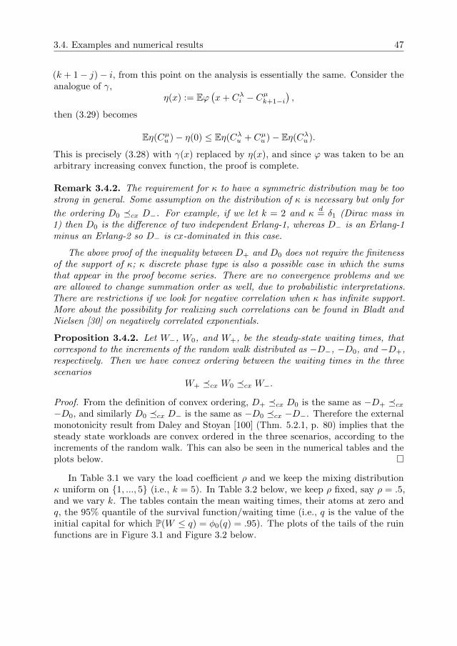
3.4. Examples and numerical results 47

(k + 1− j)− i, from this point on the analysis is essentially the same. Consider theanalogue of γ,

η(x) := Eϕ(x+ Cλi − Cµk+1−i

),

then (3.29) becomes

Eη(Cµu )− η(0) ≤ Eη(Cλu + Cµu )− Eη(Cλu ).

This is precisely (3.28) with γ(x) replaced by η(x), and since ϕ was taken to be anarbitrary increasing convex function, the proof is complete.

Remark 3.4.2. The requirement for κ to have a symmetric distribution may be toostrong in general. Some assumption on the distribution of κ is necessary but only for

the ordering D0 �cx D−. For example, if we let k = 2 and κd= δ1 (Dirac mass in

1) then D0 is the difference of two independent Erlang-1, whereas D− is an Erlang-1minus an Erlang-2 so D− is cx-dominated in this case.

The above proof of the inequality between D+ and D0 does not require the finitenessof the support of κ; κ discrete phase type is also a possible case in which the sumsthat appear in the proof become series. There are no convergence problems and weare allowed to change summation order as well, due to probabilistic interpretations.There are restrictions if we look for negative correlation when κ has infinite support.More about the possibility for realizing such correlations can be found in Bladt andNielsen [30] on negatively correlated exponentials.

Proposition 3.4.2. Let W−, W0, and W+, be the steady-state waiting times, thatcorrespond to the increments of the random walk distributed as −D−, −D0, and −D+,respectively. Then we have convex ordering between the waiting times in the threescenarios

W+ �cx W0 �cx W−.

Proof. From the definition of convex ordering, D+ �cx D0 is the same as −D+ �cx−D0, and similarly D0 �cx D− is the same as −D0 �cx −D−. Therefore the externalmonotonicity result from Daley and Stoyan [100] (Thm. 5.2.1, p. 80) implies that thesteady state workloads are convex ordered in the three scenarios, according to theincrements of the random walk. This can also be seen in the numerical tables and theplots below.

In Table 3.1 we vary the load coefficient ρ and we keep the mixing distributionκ uniform on {1, ..., 5} (i.e., k = 5). In Table 3.2 below, we keep ρ fixed, say ρ = .5,and we vary k. The tables contain the mean waiting times, their atoms at zero andq, the 95% quantile of the survival function/waiting time (i.e., q is the value of theinitial capital for which P(W ≤ q) = φ0(q) = .95). The plots of the tails of the ruinfunctions are in Figure 3.1 and Figure 3.2 below.

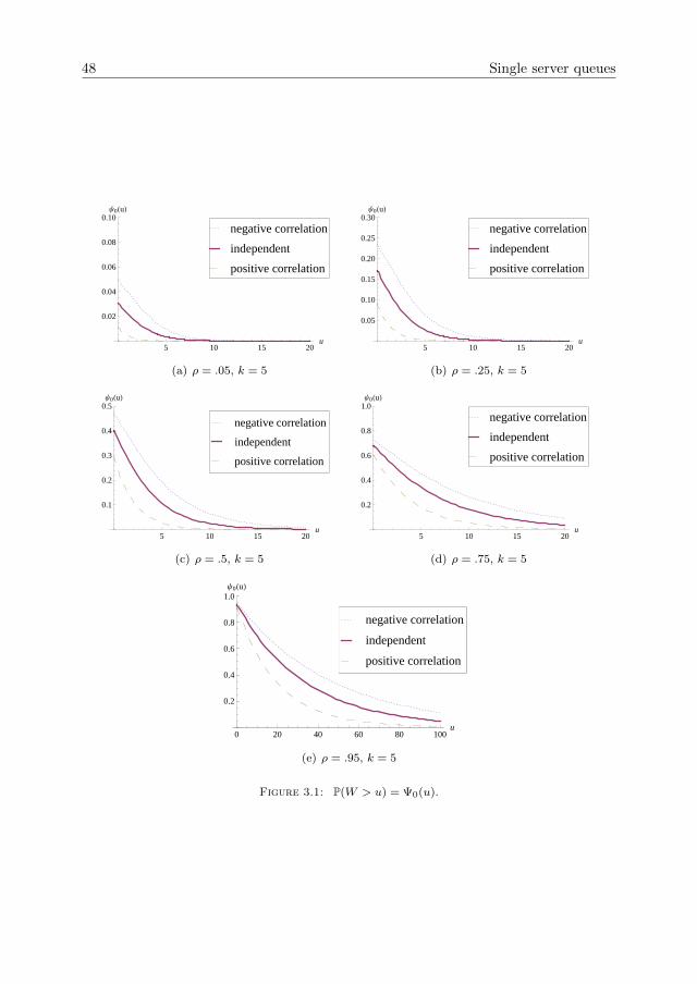
48 Single server queues

5 10 15 20u

0.02

0.04

0.06

0.08

0.10Ψ0HuL

positive correlation

independent

negative correlation

(a) ρ = .05, k = 5

5 10 15 20u

0.05

0.10

0.15

0.20

0.25

0.30Ψ0HuL

positive correlation

independent

negative correlation

(b) ρ = .25, k = 5

5 10 15 20u

0.1

0.2

0.3

0.4

0.5Ψ0HuL

positive correlation

independent

negative correlation

(c) ρ = .5, k = 5

5 10 15 20u

0.2

0.4

0.6

0.8

1.0Ψ0HuL

positive correlation

independent

negative correlation

(d) ρ = .75, k = 5

0 20 40 60 80 100u

0.2

0.4

0.6

0.8

1.0Ψ0HuL

positive correlation

independent

negative correlation

(e) ρ = .95, k = 5

Figure 3.1: P(W > u) = Ψ0(u).

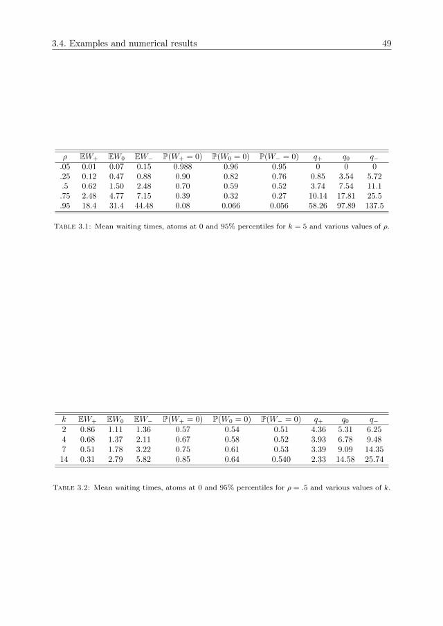
3.4. Examples and numerical results 49

ρ EW+ EW0 EW− P(W+ = 0) P(W0 = 0) P(W− = 0) q+ q0 q−.05 0.01 0.07 0.15 0.988 0.96 0.95 0 0 0.25 0.12 0.47 0.88 0.90 0.82 0.76 0.85 3.54 5.72.5 0.62 1.50 2.48 0.70 0.59 0.52 3.74 7.54 11.1.75 2.48 4.77 7.15 0.39 0.32 0.27 10.14 17.81 25.5.95 18.4 31.4 44.48 0.08 0.066 0.056 58.26 97.89 137.5

Table 3.1: Mean waiting times, atoms at 0 and 95% percentiles for k = 5 and various values of ρ.

k EW+ EW0 EW− P(W+ = 0) P(W0 = 0) P(W− = 0) q+ q0 q−2 0.86 1.11 1.36 0.57 0.54 0.51 4.36 5.31 6.254 0.68 1.37 2.11 0.67 0.58 0.52 3.93 6.78 9.487 0.51 1.78 3.22 0.75 0.61 0.53 3.39 9.09 14.3514 0.31 2.79 5.82 0.85 0.64 0.540 2.33 14.58 25.74

Table 3.2: Mean waiting times, atoms at 0 and 95% percentiles for ρ = .5 and various values of k.

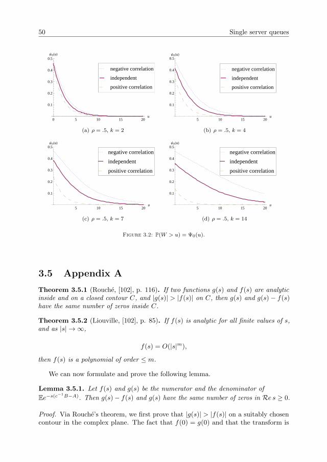
50 Single server queues

0 5 10 15 20u

0.1

0.2

0.3

0.4

0.5Ψ0HuL

positive correlation

independent

negative correlation

(a) ρ = .5, k = 2

5 10 15 20u

0.1

0.2

0.3

0.4

0.5Ψ0HuL

positive correlation

independent

negative correlation

(b) ρ = .5, k = 4

5 10 15 20u

0.1

0.2

0.3

0.4

0.5Ψ0HuL

positive correlation

independent

negative correlation

(c) ρ = .5, k = 7

5 10 15 20u

0.1

0.2

0.3

0.4

0.5Ψ0HuL

positive correlation

independent

negative correlation

(d) ρ = .5, k = 14

Figure 3.2: P(W > u) = Ψ0(u).

3.5 Appendix A

Theorem 3.5.1 (Rouche, [102], p. 116). If two functions g(s) and f(s) are analyticinside and on a closed contour C, and |g(s)| > |f(s)| on C, then g(s) and g(s)− f(s)have the same number of zeros inside C.

Theorem 3.5.2 (Liouville, [102], p. 85). If f(s) is analytic for all finite values of s,and as |s| → ∞,

f(s) = O(|s|m),

then f(s) is a polynomial of order ≤ m.

We can now formulate and prove the following lemma.

Lemma 3.5.1. Let f(s) and g(s) be the numerator and the denominator of

Ee−s(c−1B−A). Then g(s)− f(s) and g(s) have the same number of zeros in Re s ≥ 0.

Proof. Via Rouche’s theorem, we first prove that |g(s)| > |f(s)| on a suitably chosencontour in the complex plane. The fact that f(0) = g(0) and that the transform is

3.5. Appendix A 51

rational (so it is also analytic on a strip in Re s < 0) suggests that we consider thefollowing contour made up from the extended semi-circle

Cε := {R(cosϕ+ i sinϕ); ϕ ∈ [−π/2− arccos ε, π/2 + arccos ε]} ,

together with the vertical line segment S :={−ε+ iω; |ω| ∈

[0, R√

1− ε2]}.

We show that |g(s)| > |f(s)| on this contour, for ε sufficiently small.

First on Cε:∣∣∣ f(Reiϕ)g(Reiϕ)

∣∣∣ ≤ Ee−R cosϕ(c−1B−A) → P(c−1B −A = 0) as R→∞.

We can assume P(A = c−1B) < 1, else there is nothing to prove. This means

| f(Reiϕ)g(Reiϕ) | < 1 for R sufficiently large.

In order to prove the inequality on the line segment S, we use the stability condition:

E(A− c−1B) = ddsf(s)g(s) |s=0 > 0. So for ε sufficiently small, f(−ε)

g(−ε) <f(0)g(0) = 1. Then on

S we have:∣∣∣∣f(−ε+ iω)

g(−ε+ iω)

∣∣∣∣ = |Ee−(−ε+iω)(c−1B−A)| ≤ Eeε(c−1B−A)|e−iω(c−1B−A)| = f(−ε)g(−ε) < 1.

Hence |f(s)| < |g(s)| on the whole contour. These being polynomials, Rouche’stheorem 3.5.1 ensures that g and g − f have the same number of zeros inside Cε, andsince ε was arbitrarily small, this also holds on ∩ε>0C◦ε = {s; Re s ≥ 0}∩{s; |s| ≤ R},where C◦ε is the interior of Cε. Finally, letting R→∞, proves the assertion.

Proof of Lemma 3.4.1. a) We can write the joint Laplace-Stieltjes transform byconditioning on κ:

Ee−s1A−s2B =

∞∑n=1

P(κ = n)

(λ

λ+ s1

)n(µ

µ+ s2

)n.

If we set z = λλ+s1

µµ+s2

, we can recognize the probability generating function of κ at

z, call it Pκ(z).κ has a discrete phase-type distribution with representation (α, T ) (Neuts [90]),

such that I − T is non-singular (here I is the identity matrix), and the probabilityvector α is supported on the transient states. Thus

P(κ = n) = α′Tn−1t

for n ≥ 1, t = (I − T )1, P (κ = 0) = 0. If we now focus on this generating function,we have the following (Asmussen [16] Prop. 4.1, p. 83):

Pκ(z) = α′(z−1I − T )−1t,

and we have proved part a).b) To see why Ee−sX = Pκ( λ

λ−sµµ+s ) is a rational function, rewrite the inverse :

(z−1I − T )−1 =1

det(z−1I − T )(z−1I − T )∗.

Remark that the denominator det(z−1I − T ) is a polynomial of order |S| − 1 (thenumber of transient states) in z−1, because z−1 appears only on the diagonal of the

52 Single server queues

matrix (z−1I−T ). (z−1I−T )∗ is the algebraic complement of (z−1I−T ) (also knownas matrix of cofactors). Its entries are of the form (−1)i+j det(Mij), where Mij is thematrix obtained by deleting row i and column j of (z−1I − T ). These are polynomialsin z−1 of order < |S| − 1 (because of the deleted rows and columns in the entries, thedegree of the determinants of these sub-blocks as polynomials in z−1 is always smallerthan the dimension of the matrix T ) and hence so is the bilinear form α′(z−1I − T )∗t,which is the numerator of Pκ(z).

Lemma 3.5.2. φ(w) in (3.17) is differentiable.

Proof. Let hw(v) :=w+cv∫x=w

x∫z=0

fA,B(v, z)φ0(x− z) dz dx. Using the triangle inequality,

we have the following upper bound

|hw+ε(v)−hw(v)| ≤w+ε∫w

x∫0

fA,B(v, z)φ0(x−z) dz dx+

w+cv+ε∫w+cv

x∫0

fA,B(v, z)φ0(x−z) dz dx.

Let us denote by I and II the first and the second term that appear above, respectively.If we use the fact that φ0(x) ≤ 1, we find the upper bounds on I and II:

I ≤w+ε∫x=w

w+ε∫z=0

fA,B(v, z) dz dx = ε

w+ε∫z=0

fA,B(v, z) dz,

and similarly,

II ≤ εw+cv+ε∫z=0

fA,B(v, z) dz.

So if we denote Dε(v) := hw+ε(v)−hw(v)ε ,

|Dε(v)| ≤w+ε∫z=0

fA,B(v, z) dz +

w+cv+ε∫z=0

fA,B(v, z) dz ≤ 2fA(v),

and clearly the upper bound is integrable as a function of v. By virtue of dominatedconvergence

φ′(w) = limε→0

∞∫v=0

Dε(v) dv =

∞∫v=0

limε→0

Dε(v) dv =

∞∫v=0

∂

∂whw(v) dv.

Lemma 3.5.3. Under the conditions from Remark 3.3.1, the density of the pair(Ares, B∗) is

f(Ares,B∗)(r, z) = α

∞∫v=r

f(A,B)(v, z) dv.

3.5. Appendix A 53

Proof. Consider the augmented pair (A, B∗) which by definition has density

f(A,B∗)(v, z) := αvfA,B(v, z),

where α acts as the normalizing factor: 1α = EA =

∫z

∫vvfA,B(v, z) dv dz. Let U be a

standard uniform r.v., independent of both A and B. Then (Ares, B∗)d= ((1−U)A, B∗),

therefore conditional on A, Ares is uniformly distributed over the interval [0, A], so wemay write in terms of density functions

f(Ares,B∗)(v, z) =

∞∫r=v

1

rf(A,B∗)(r, z) dr = α

∞∫r=v

f(A,B)(r, z) dr.

The proof is complete.

Chapter 4

Integral representations forone-dimensional randomwalks

A usual assumption in the theory of fluctuations of random walks as they appear in,e.g., queueing or insurance applications, is that the increment of the random walkcan be represented as the difference of two independent random variables. In thecontext of queueing theory, random walks with increments which do not have thisproperty appear as embedded at arrival epochs of customers in a GI/G/1 queue inwhich the service requirement of the current customer is correlated with the time untilthe next arrival. In risk reserve processes that appear in insurance, the independenceassumption is violated when the current claim size depends on the time elapsed sincethe previous arrival, and hence on the premium gained meanwhile. A useful relationbetween the queueing system and the risk reserve model is given via the dualityrelation described at the end of Section 1.3.

The purpose of the present chapter is to show how much can be done for randomwalks which do not satisfy this independence assumption, regarding their maxima (asin the waiting time/maximum aggregate loss), their minima (idle periods/deficit atruin) and their excursions (related to busy periods/time to ruin).

From a queueing perspective, it turns out that the busy period is a more sensitiveissue to study than the idle period or the waiting time, as it appears from the proof ofTheorem 4.2.1 below. For this purpose, we present a generalization of an inversionformula for characteristic functions/Fourier-Stieltjes transforms due to Hewitt [69],which in turn is an extension of P. Levy’s inversion formula. All these results areessentially variations on the Dirichlet integral for complex-valued functions of boundedvariation.

From a stochastic point of view, the information contained by the increments ofthe random walk is sufficient to infer about the extreme statistics; and since successiveincrements are independent, the usual form of Hewitt’s inversion formula is sufficientto obtain the integral representations; this is how it was used originally by Spitzer

55

56 Integral representations

[99] to derive the Laplace-Stieltjes transform of the maxima of partial sums. He alsorelated these transforms to the Wiener-Hopf problem (see in addition Cohen [40],Ch. II.5, for the relation with the Wiener-Hopf equation as it appears in ProbabilityTheory). For the derivation of the length of an excursion above the starting level,there is more information needed, namely, that given by the partial sums

∑ni=1Bi

together with the partial sums of the embedded random walk Sn =∑ni Bi−

∑ni Ai. It

is possible to derive the excursion lengths still using Hewitt’s formula when the Ai’sare independent of the Bi’s, and this was carried out in Kingman [74]. It is shown inthe present chapter that if one extends Hewitt’s inversion formula, a similar derivationis possible for the case when there is arbitrary correlation inside the vectors (Ai, Bi),which means the random walk Sn can have generally distributed increments.

Hewitt’s approach was to find a most general inversion identity for Laplace-Stieltjestransforms with a view on Harmonic Analysis; this is much more than we need forour purposes. Instead of trying to find a most general instance of inversion, the focusin the present chapter is to obtain a sufficiently broad result to apply to the kind ofrandom walks that appear in the study of workload/insurance related problems. Onecan only hope then that the result itself will find applications in other related areas ofprobability and statistics.

In the queueing literature, Conolly obtained (the transform of) the busy periodtogether with the number of customers served in an Erlang queue with independentexponential inter-arrivals [46], and he obtained continued fraction expansions for theErlang queue with state dependent parameters of both the exponential inter-arrivalsand the service times in [47]. Conolly’s results from [46] were then extended to generalindependent inter-arrivals and service times in Finch [58] and in Kingman [74].

The time to ruin has been studied in the insurance literature by deriving recursionformulae, typically obtained by discretising the claim sizes. For example, Dickson andWaters [50] present various approximation methods for its numerical computation.Studying the time to ruin is analytically the same as inferring on the busy period,by virtue of the alternative form of duality, see the end of Section 1.3. Anothergood reference is Prabhu [93] §3, who obtained an integral equation for the time toruin starting from a positive capital u, in the Cramer-Lundberg risk reserve model;Borovkov and Dickson [32] obtain series representations for the distribution of the timeto ruin in the Sparre-Andersen risk reserve model with exponentially distributed claimsand general renewal inter-arrivals. Besides these results, there exists a significantamount of literature on the Gerber-Shiu functions which contain the time to ruin asa special case. We will come back to the problem of analyzing the time to ruin inSection 4.4.

The chapter is organized in the following way: In Section 4.1, we extend Hewitt’sinversion formula to allow for probability distribution functions on R2 which do nothave a product form (see Remark 4.1.1). One of the ingredients of the proof consistsof having a precise meaning for the conditional distribution of B given A; this issettled as a preliminary. The approach used for studying fluctuations of random walksinvolves obtaining integral representations for the above-mentioned quantities. Thebusy period, idle period, transient workload, and the related insurance functionals canstill be determined in the form of a Cauchy integral, once Theorem 4.1.1 is combinedwith a version of Spitzer-Baxter’s identity (Proposition 4.2.1), and this is carried out

4.1. On Hewitt’s inversion formula 57

in detail in Section 4.2 for the correlated GI/G/1 queue and the Sparre-Andersen riskreserve process. Roughly speaking, all the transforms of the relevant performancemeasures are obtained by reading the inversion formula in Theorem 4.1.1 from rightto left. The combination of Spitzer-Baxter’s identity with Hewitt’s inversion has beenused by Kingman [74] to determine busy periods when inter-arrivals are independentfrom service requirements.

Having obtained a Cauchy integral representation for the busy period, one canthen evaluate it when the transform of the generic pair (B,A) is a rational function inthe argument that corresponds to the service requirement B (Section 4.3). Finally, wepoint out in Section 4.4 how one can obtain the distribution of the time to ruin in thedual risk setting, when starting with a non-negative initial capital.

4.1 On Hewitt’s inversion formula

The starting point is P. Levy’s inversion formula which gives a precise form to thewell known assertion that a characteristic function uniquely determines a probabilitymeasure φ on the real line:

limT→∞

1

2πi

iT∫−iT

∞∫−∞

eξxφ(dx)

e−ξa − e−ξbξ

dξ =1

2φ((a, b)) +

1

2φ((a, b]).

Thus the value φ((a, b]) :=∫χ(a,b](u)φ(du) can be recovered, χ(a,b] being the indicator

function of the interval (a, b]. Hewitt’s formula extends this result to recover directlyfunctionals of the form

φ(f) :=1

2

∫[f(u+) + f(u−)]φ(du),

for functions f of bounded variation; if f is also continuous, then the integral abovebecomes

∫f(u)φ(du).

The inversion formula in the form given by Levy is further generalized to higherdimensions and some other topological groups in Hewitt [69]. It is not however thepurpose of the current chapter to explore the possibility of a most general form for it.Such an attempt may not even yield satisfactory results, as was already pointed outin [69].

We will generalize the above in Theorem 4.1.1 to probability measures on R2

related to the random vector (B,A). The probabilistic structure is never really lost,the conditional distribution of B given A appears throughout the proof of Theorem4.1.1 disguised as the conditional kernel q(u, y), which is defined below as a ”partial”Radon-Nikodym derivative.

4.1.1 Preliminaries

We say that f : R→ C is of bounded variation if both its real and imaginary partsare of bounded variation; this is the same as |f | being of bounded variation because

58 Integral representations

all norms are equivalent on C. We will also work with (complex-valued) measures onthe Borel subsets of R2, which are of finite total variation. For such a measure φ, wewill denote by |φ| the total variation measure of φ, and with ‖φ‖ its total variation.This will suffice for our purposes, but this set-up is fully detailed and generalized in[69], and the references therein.

Let (B,A) be a random vector on some probability space, having an arbitraryprobability distribution. Denote by P the probability measure and by H the joint c.d.f.of (B,A):

H(x, y) = P(B ≤ x, A ≤ y).

The correlation device for the increment of the random walk is given by this distribution,not necessarily having a product form, and its Fourier-Stieltjes transform

h(s1, s2) := Ee−s1B−s2A =

∫e−s1x−s2yH(dx, dy).

In general this is convergent only for Re s1 = 0, Re s2 = 0, but if (B,A) is supportedon the non-negative quadrant in R2, then h can be continued analytically to Re s1 ≥0, Re s2 ≥ 0. The characteristic function of the increment A−B will also be relevant:

h(ξ,−ξ) =

∫eξx dP(A−B ≤ x), Re ξ = 0.

Let λ be the probability measure associated with the random vector (B,A), and νbe the marginal measure associated with B,

λ(U × V) := P(B ∈ U , A ∈ V), ν(U) := λ(U × R), U ,V ∈ B(R),

with B(R) the family of Borel sets on the line. The notation H(du, y) will be used tosuggest that we are integrating w.r.t. the measure λy(U) := λ(U × (−∞, y]). We willwork with a version of the conditional cumulative distribution function (c.d.f.) of Agiven B and this is made precise below.

It clearly holds that λy(U) ≤ ν(U), in particular λy � ν, so let

q(u, y) :=dλydν

(u)

be its Radon-Nikodym derivative. Heuristically, q(u, y) is to be regarded as q(u, y) =P(A ≤ y |B ∈ du), and we have the disintegration identity∫

UH(du, y) ≡ H(U , y) ≡

∫Uq(u, y) ν(du),

with any of the terms above meaning P(A ≤ y, B ∈ U). We will be working with aregular version of q, which exists by virtue of the separability of R, see for instanceKallenberg [72] Thm. 5.3, p. 84. Further, we have more than just regularity for thiskernel, the same result gives that q(u, y) is regularly monotone as a function in theargument y, i.e., q(u, y) is non-decreasing in y outside a set of ν−measure zero whichdoes not depend on y.

4.1. On Hewitt’s inversion formula 59

These considerations are quite intuitive because of the probabilistic nature of themeasure associated with H. It turns out, however, that we will have to considerinstances of the inversion theorem for the slightly more general case of complex valuedfunctions H which are also of bounded variation, and for this purpose we will showbelow that H(du, x) can be given a meaning in an analogous way.

Confusing H with its associated complex-valued measure, see Hewitt [69], we canreduce it to a monotonically increasing function, by splitting into real and imaginaryparts and using the Jordan decomposition

ReH ≡ (ReH)+ − (ReH)−,

for the signed measure ReH, and similarly for ImH. Setting ν±(U) := (ReH)±(U ×R), it holds with the similar notation as in the probabilistic case that (ReH)±y � ν±,so we can define again the Radon-Nikodym derivatives

q+1 (u, y) :=

d(ReH)+y

dν+(u), q−1 (u, y) :=

d(ReH)−ydν−

(u),

and similarly for ImH. Now we can reconstruct H(du, y) in an obvious way, usingthe linearity of the Radon-Nikodym derivative.

Alternatively, we could have used the total variation measures:

|ReHy|(U) ≤ |ReH|(U × R)

and thusReHy � ν, but a simple argument relying on the Hahn-Jordan decompositionshows that this construction yields the same result for H(du, x).

Moreover, the monotone regularity property from the probabilistic instance extendsto q(u, y) being of bounded variation in y outside a set of ν-measure zero which doesnot depend on y. This property will be useful in the proof of the next result.

Theorem 4.1.1 (Generalized Hewitt inversion). Let H be a totally bounded(complex-valued) measure on R2, and let f : R→ C be a function of bounded variationwhich is also absolutely integrable (w.r.t. the Lebesgue measure). Then the followingCauchy principal value can be represented as a Lebesgue-Stieltjes integral:

limT→∞

1

2πi

iT∫−iT

∞∫−∞

∞∫−∞

eξ(u−y)H(du,y)f(y)dy

dξ

=1

2

∞∫−∞

{f(u+)H(du, u+) + f(u−)H(du, u−)} .

f need not be integrable w.r.t. H(du, u). If one of the sides above converges, so doesthe other one.

Remark 4.1.1. If H is of the form H1H2, the double integral inside the Cauchyprincipal value factorizes into the Fourier-Stieltjes transform of H1 and the Fouriertransform of f(y)H2(y), this function being again absolutely integrable and of bounded

60 Integral representations

variation. Thus the above reduces to the inversion formula in Hewitt [69], Thm.(3.1.1):

limT→∞

1

2πi

iT∫−iT

∞∫−∞

eξuH1(du)

∞∫−∞

e−ξyg(y) dy

dξ =1

2

∞∫−∞

[g(u+)+g(u−)]H1(du),

with g(y) = f(y)H2(y).

Proof of Theorem 4.1.1. For fixed u, change the variable x := u−y, so that the doubleintegral inside the Cauchy principal value becomes

∞∫−∞

∞∫−∞

eξ(u−y)H(du, y)f(y) dy =

∞∫−∞

∞∫−∞

eξxH(du, u− x)f(u− x) dx.

We can bound

∫dx

∣∣∣∣∫ H(du, u− x)f(u− x)

∣∣∣∣ ≤ ∫ dx

∫|f(u− x)| |H|(du,∞) = ‖H‖

∫|f(v)|dv,

hence∫H(du, u− x)f(u− x) is absolutely integrable in x because f is. We can now

change the order of integration in the Cauchy principal value, which becomes afterintegrating over ξ:

limT→∞

∫∫1

2πi

iT∫−iT

eξx dξ H(du, u−x)f(x)dx= limT→∞

∫sinTx

πxdx

∫H(du, u−x)f(u−x).

(4.1)At this point, disintegrate the kernel H(du, u− x) = q(u, u− x) ν(du), so that, by

the Radon-Nikodym Theorem, we can rewrite the right-hand side in (4.1) as

limT→∞

∫ν(du)

{∫sinTx

πxq(u, u− x)f(u− x) dx

}. (4.2)

The main remark is that q(u, u− x)f(u− x) is of bounded variation as a function inx for ν-almost all u, but regularity is the key, as can be seen from the following:

Let {xi}i∈I be some ordered sequence determined by the edges of an intervalpartition of R. Since f is assumed of bounded variation, it can be reduced to a realvalued and monotonically increasing function, again by splitting it into its real andimaginary parts and making use of Jordan’s decomposition. Similarly, q(u, ·) can bereduced to a regularly non-decreasing function. Then we can write by exploiting themonotonicity of both q(u, ·) and f :

m∑i=1

[q(u, u− xi)f(u− xi)−q(u, u− xi+1)f(u− xi+1)]

4.2. The GI/G/1 queue with correlations 61

≤∞∑i=1

q(u, u− xi)[f(u− xi)− f(u− xi+1)]

≤ q(u,∞)

m∑i=1

[f(u− xi)− f(u− xi+1)], u /∈ Q,

where, by virtue of the regularity of q, Q is a ν−negligible set, outside which q(u, ·) ismonotone.

Notice that in the upper bound the arguments of q do not depend anymore on thepartition {xi}i. Even more so, q(u,∞) = 1 ν−a.e. by definition. Since by regularity,Q does not depend on the sequence (xi)i, we can take the supremum over all suchsequences and using that f is of bounded variation, gives that also q(u, u− x)f(u− x)is of bounded variation for ν−almost all u.

We have arrived at the following limit:

limT→∞

∞∫−∞

sinTx

πxϕ(u, x) dx =

1

2[ϕ(u, 0+) + ϕ(u, 0−)],

for fixed u and ϕ(u, x) := q(u, u− x)f(u− x). This identity is known as Dirichlet’sintegral. The integrability condition for the left-hand side that assures the limit existsis that ϕ(u, ·) be of bounded variation. As seen from the above, this assumption is onlyslightly more general than Dirichlet’s original condition of monotonicity for ϕ(u, ·).See Doetsch [51] Ch. 24, or Titchmarsh [102] §13.2 (the condition is also known asJordan’s test). The limit equals what is usually called the normalized function in theorigin.

The proof will be complete as soon as we show that the limit in T can be takeninside the ν(du) integral (4.2). Reduce f again to a non-negative and monotonicallyincreasing function. Using the second mean value theorem for ϕ(u, x) which is nowdecreasing in x, for some β > 0, we can find α > 0 such that∣∣∣∣∣∣

β∫0

ϕ(u, x)sinTx

xdx

∣∣∣∣∣∣ ≤∣∣∣∣∣∣ϕ(u, 0)

α∫0

sinTx

xdx

∣∣∣∣∣∣ < ϕ(u, 0)

π∫0

sinx

xdx.

The final upper bound is obtained by a change of variable x→ x/T . This is the sameargument as given in Hewitt [69], and it is clearly sufficient to allow the interchangingof limit and integration in (4.2); this together with the fact that Dirichlet’s integralidentity holds for ν-almost all u, completes the proof.

4.2 The GI/G/1 queue with correlations

Having laid down the inversion result in the previous section, let us start with thestudy of the special queueing system GI/G/1 briefly described in the introduction.

It is assumed that the law of the random walk {Sn}n≥0

62 Integral representations

Sn = S0 +

n∑i=1

(Bi −Ai)

is the law P conditional on S0 = 0. Also set bn =∑ni=1Bi and an =

∑ni=1Ai.

Let N be a random variable which is distributed as the number of customers servedduring a busy cycle of the server. Then (assuming unit server speed) bN , aN , −SNstand for the length of the busy period, that of the busy cycle and respectively theidle time of the server.

In queueing terms, one can think of the pair (B,A) as the service time of a genericcustomer together with the time until the arrival of the next customer in a GI/G/1queueing system - which can be always normalized to unit server speed without losinggenerality. In terms of insurance and risk theory, this pair can be interpreted as thetime elapsed (and hence the premium B gained) since the last claim incurred togetherwith the amount A claimed through an insurance policy. Then, conditional on startingwith 0 initial capital, bN is the time to ruin (after normalizing the risk reserve processin order to have unit income rate), aN is the total amount claimed until ruin (includingthe claim that causes it) and −SN is the deficit at ruin.

The representation given below was obtained in Wendel [103] §4 as an algebraicidentity, slightly more general than Spitzer’s identity, who originally obtained in [99]the representation for the LST of the successive maxima of the partial sums (Sn)n (seealso Baxter and Donsker [28] for a similar derivation that holds for Levy processes).Theorem 1 and Identity (9) in Kingman [74] are much closer to our purposes. For thesake of completeness, we cite the relevant result in the following proposition

Proposition 4.2.1 (Spitzer, Wendel, Baxter). With the above notations, it holds that

E{zNe−s1bN−s2SN } = 1− exp

{−∞∑n=1

zn

nE[e−s1bn−s2Sn1{Sn<0}]

}, (4.3)

which holds for Re s1 ≥ 0, Re s2 ≤ 0, |z| ≤ 1.

In Kingman [74], this identity is obtained by ’killing’ inside the Spitzer-Wendelidentity, i.e. in the three-dimensional space where (an, bn, Sn)n is evolving, replacethe reflecting hyperplane at x3 = 0 with an absorbing hyperplane. This is formallycarried out in [74] by replacing the projection operator used by Wendel [103] with anabsorption operator.

We will use Theorem 4.1.1 in conjunction with the version of Spitzer’s identityfrom Proposition 4.2.1 to obtain integral representations for the transforms of thebusy period, idle period and the number of customers served during a busy period.

Throughout the rest of this chapter, we will use the dashed integral sign as areplacement for the cumbersome limit

limT→∞

iT∫−iT

≡ −i∞∫−i∞

.

4.2. The GI/G/1 queue with correlations 63

Theorem 4.2.1. We have the following integral representations for P := bN , I :=−SN , valid whenever Re s > 0, |z| < 1:

E{zNe−sP } = 1− exp

1

2πi−i∞∫−i∞

dξ

s− ξ {log[1− zh(ξ, 0)]− log[1− zh(ξ, s− ξ)]}

,

(4.4)

E{zNe−sI} = 1− exp

1

2πi−i∞∫−i∞

dξ

s+ ξlog[1− zh(ξ,−ξ)]

. (4.5)

Here log is the principal branch, that has the cut taken along the negative real axisbetween 0 and ∞, so that it admits the power series representation

log1

1− r =

∞∑n=1

rn

n, |r| < 1.

Proof. Below we will use an integration by parts argument and for this reason it willbe convenient to introduce the function G(u, x) = P(B ≤ u,A > x). We can write byintegrating over the possible values of bn:

P(bn < an) =

∞∫0

G∗n(dx, x) and P(bn ≤ an) =

∞∫0

G∗n(dx, x−)

where G∗n(x, y) := P(bn ≤ x, an > y), is the n-fold convolution of G with itself andG∗n(dx, y) is the associated integral kernel, as described in Section 4.1,

G∗n(dx, y) ≡ P(bn ∈ dx, an > y), G∗n(dx, y−) ≡ P(bn ∈ dx, an ≥ y).

Let us begin with (4.4), which means we start with (4.3) for s2 = 0 and s1 = s.The first step is to represent the expected value inside the series in (4.3):

1

2E[e−sbn(1{Sn≤0} + 1{Sn<0})] =

∞∫0

e−sx[1

2G∗n(dx, x−) +

1

2G∗n(dx, x+)]. (4.6)

Define the following z-harmonic measure associated to G(dx,dy) = −H(dx,dy):

H∗z (dx, dy) =

∞∑n=1

zn

nG∗n(dx, dy),

so that, in particular,

H∗z (dx, y) =

∞∑n=1

zn

nG∗n(dx, y). (4.7)

64 Integral representations

H∗z is a complex valued measure proper (i.e. it has finite total variation) for |z| < 1,since we have

||H∗z || ≤∑n=1

|z|nn

= log1

1− |z| ;

moreover, its LST equals∫e−s1x−s2yH∗z (dx,dy) =

∞∑n=1

zn

nhn(s1, s2), (4.8)

where the interchanging of the integral with the series is allowed because of absoluteintegrability:

∫∫|e−s1x−s2y| |H∗z |(dx, dy) ≤

∞∑n=1

|z|nn

∫∫G∗n(dx, dy) = log

1

1− |z| .

Now let us use Theorem 4.1.1 for f(y) = e−syχ[0,∞)(y), Re s > 0, which means wecan write via (4.6) and (4.7):

∞∑n=1

zn

nE[e−sbn(1{Sn≤0} + 1{Sn<0})] =

1

2πi−i∞∫−i∞

∞∫

0

∞∫0

eξx−(s+ξ)yH∗z (dx, y) dy

dξ.

(4.9)Assume for simplicity that P(A = B) = 0 (i.e. P(Sn = 0) is null for all n). This

assumption is not essential, see for example the discussion in Cohen [40], p. 284. Thenthe normalized indicator function 1

2 (1{Sn≤0} + 1{Sn<0}) that appears on the left-handside of (4.6) simplifies to 1{Sn<0}. Since H∗z (dx, y) is of bounded variation in y, wecan use the integration by parts formula for Lebesgue-Stieltjes integrals, so that (4.9)becomes

1

2πi−i∞∫−i∞

dξ

s+ ξ

∞∫

0

eξx

H∗z (dx, 0−) +

∞∫y=0

e−(s+ξ)yH∗z (dx, dy)

=

1

2πi−i∞∫−i∞

dξ

s+ ξ

[ ∞∑n=1

zn

nhn(−ξ, 0)−

∞∑n=1

zn

nhn(−ξ, s+ ξ)

], (4.10)

where we used (4.8) and the identity G(x, 0−) = P(B ≤ x). Changing the variableξ → −ξ, the exponent in (4.3) can be rewritten via (4.10), for Re s > 0, |z| < 1:

−∞∑n=1

zn

nE[e−sbn1{Sn<0}] =

1

2πi−i∞∫−i∞

dξ

s− ξ {log[1− zh(ξ, 0)]− log[1− zh(ξ, s− ξ)]} .

(4.11)

4.2. The GI/G/1 queue with correlations 65

Thus (4.4) follows from these considerations and Spitzer’s identity (4.2.1).

For the integral representation (4.5), the extension of Hewitt’s formula is notneeded. The starting point is (4.3) with s1 = 0, s2 = −s, Re s > 0, together with theidentity

EesSn1{Sn<0} =1

2

0+∫−∞

esxdP(Sn ≤ x) +1

2

0−∫−∞

esxdP(Sn ≤ x)

valid because P(S1 = 0) = 0. Similarly as above, set F (x) = P(S1 ≤ x) and introduce

F ∗z (dx) :=

∞∑n=1

zn

nF ∗n(dx). (4.12)

Use the inversion formula in Remark 4.1.1 with g(y) = esyχ(−∞,0](y), Re s > 0, sothat we can write similarly as for (4.9)-(4.10):

∞∑n=1

zn

nEesSn1{Sn<0} =

1

2πi−i∞∫−i∞

∞∫−∞

eξxF ∗z (dx)

0∫−∞

e(s−ξ)y dy

dξ

=1

2πi−i∞∫−i∞

dξ

s− ξ∞∑n=1

zn

nhn(−ξ, ξ)

=− 1

2πi−i∞∫−i∞

dξ

s+ ξlog[1− zh(ξ,−ξ)], Re s > 0, (4.13)

after the change of variable ξ → −ξ.Once (4.13) is replaced into (4.3), it immediately yields (4.5). The proof is complete.

Remark 4.2.1. If B is independent of A, then h(s1, s2) is the product of the marginaltransforms and the integral representation (4.4) reduces to that from Kingman [74],Thm. 4 (see also Cohen [40], p. 304 for (4.5)).

Remark 4.2.2. The integral representations (4.4) and (4.5) hold under very generalconditions (there are no regularity assumptions of the distribution of (B,A), thesecan even be discrete random variables, in which case the LSTs become generatingfunctions). The reason is that these representations are given for the interior of theirconvergence domains (Re s>0, |z|<1). If we want to take any of the arguments totheir respective boundary, we have to require extra conditions to ensure convergence.For example, when letting s converge towards the imaginary axis, there is a singularityappearing, because the factor 1/(ξ − s) gains a simple pole located at ξ=s.

It turns out one can give a definite meaning to these integrals, for Re s= 0, ifthey are regarded as singular integrals w.r.t. the Cauchy kernel 1/(ξ − s). Then oneconsiders the Cauchy principal value obtained by removing a circle of arbitrarily smallradius around the singularity s and then taking its radius to 0. Now we are dealing

66 Integral representations

with a double principal value: first one coming from the pole at s of the Riemannintegral along the segment L := [−iT, iT ] (T large enough, so that s ∈ L) and thesecond one obtained by letting T → ∞. A standard condition (see Gakhov [65],Muskhelishvili [87]) that ensures the first principal value converges is that the densityfunctions ϕ1(ξ) := log[1−h(ξ,−ξ)], ϕ2(s, ξ) := log[1−h(ξ, s−ξ)] are Holder continuousalong the imaginary axis, with some positive indices. The Holder continuity of ϕ1(ξ) isfairly close to Spitzer’s [98] integrability condition, which requires (upon taking s→ 0)that (1− h(ξ,−ξ))/ξ be integrable in a neighbourhood of s=0 on the imaginary axis.

4.2.1 The number of arrivals during an excursion

Further along the lines of Remark 4.2.2, we will use the doubly dashed integral sign todenote the double Cauchy principal value. The choice for the branch of log is essentialfor the definiteness of the first principal value. It turns out to be convenient to workwith a branch of log which has the cut between 0 and ∞ taken inside the negativehalf-plane (the same principal branch as the one used in Theorem 4.2.1), so we haveby definition,

1

2πi−∫L

ϕ(ξ)

ξ − sdξ := −1

2ϕ(s)+

ϕ(s)

2πi[log(iT −s)− log(−iT −s)]+ 1

2πi

∫L

ϕ(ξ)− ϕ(s)

ξ − s dξ.

(4.14)The integral on the right is well defined as a Riemann integral as soon as ϕ(s)is Holder continuous along the line L. By choice of logarithm, the argument oflog(iT − s)− log(−iT − s) equals πi for all T . This means that the first two termscancel in the limit T →∞, and the above definition becomes

1

2πi=

i∞∫−i∞

ϕ(ξ)

ξ − sdξ =1

2πi−i∞∫−i∞

ϕ(ξ)− ϕ(s)

ξ − s dξ. (4.15)

Formula (4.14) differs slightly from the definition given in Mushkelishvili [87], p.27 or Gakhov [65], p. 16, because therein the cut of the logarithm is taken in theopposite half-plane. To be more precise, in our case, Cauchy’s integral representationreads:

−i∞∫−i∞

dξ

ξ − s =

2πi, s ∈ L+,0, s ∈ L−,0, s ∈ L.

The first two values are the well known Cauchy integral identities; the third one isthe Cauchy principal value for this specific choice of log (use (4.15) with ϕ ≡ 1).

It helps to think about the Riemann sphere as the one point compactificationof the complex plane so that the imaginary axis is closed into a large circle on thesphere. Then all of the conventions above are specifying a means of integrating on thelarge circle of the sphere, the integrands being extended by continuity at infinity; the

4.2. The GI/G/1 queue with correlations 67

interior of the imaginary axis is by definition the left hemisphere and the exterior isthe right hemisphere. Define

Φ(s) = −i∞∫−i∞

ϕ(ξ)

ξ − sdξ, s ∈ C,

and the integral is defined in the sense of (4.15), when Re s = 0. If we denote byΦ−(s) the limit as s approaches the imaginary axis from its exterior, and by Φ+(s),the limit taken from the interior, then the Plemelj–Sokhotski formulae (cf. Gakhov[65], p. 25) become with the above conventions:

Φ−(s) = Φ(s), Φ+(s) = Φ(s) + ϕ(s), Re s = 0. (4.16)

Now we can calculate the limit as s approaches the imaginary axis from its exterior in(4.4), and from its interior in (4.5), using (4.16). Still denoting the interior limit withΦ+(s), (4.5) becomes for |z| < 1 and as s tends to the imaginary axis:

Φ+(s) = 1− [1− zh(−s, s)] exp

1

2πi=

i∞∫−i∞

dξ

ξ + slog[1− zh(ξ,−ξ)]

. (4.17)

Before we give the limiting values of (4.4), we point out how one can simplify it.Consider the first integral in the exponent of (4.4):

Ψ(η) := − 1

2πi−i∞∫−i∞

dξ

ξ − η log[1− zh(ξ, 0)], Re η > 0.

The key remark is that h(ξ, 0) = Ee−ξB is analytic for Re ξ > 0 and this implies thatthe density log[1− zh(ξ, 0)] is again analytic for Re ξ > 0. Since the integrand has asimple pole in the positive half-plane located at η = ξ, it follows at once from Cauchy’sTheorem applied to the imaginary axis that Ψ(η) equals

Ψ(η) = log[1− zh(η, 0)],

for any Re η > 0. This can be seen by closing the segment [−iT, iT ] with the halfcircle spanning between its endpoints inside the positive half-plane. The contourintegral thus obtained equals log[1 − zh(s, 0)] for T large enough, so that the poleη = ξ lies inside the contour (remark that because of the conventions on the interior ofthe imaginary axis, this contour is traversed in the clockwise direction). Finally, thecontribution along the half-circle tends to 0 as T →∞ because the integrand behavesas o(|ξ|−1) along the half-circle.

Having settled the first term in the exponent of (4.4), we can use the Plemelj–Sokhotski’s formula (the continuity of the exterior limit from (4.16)) for the otherterm, to obtain the identity

68 Integral representations

Φ−(s) = 1−exp

log[1− zh(s, 0)] +1

2πi=

i∞∫−i∞

dξ

ξ − s log[1− zh(ξ, s− ξ)]

, Re s = 0,

(4.18)hence we can rewrite (4.18) as

Φ−(s) = 1− [1− zh(s, 0)] exp

1

2πi=

i∞∫−i∞

dξ

ξ − s log[1− zh(ξ, s− ξ)]

, Re s = 0.

(4.19)In particular, for s = 0, the two limits (4.17) and (4.19) agree and these must then

coincide with the generating function of N . The following has been proven

Proposition 4.2.2. With the above notations and conventions, it holds for |z| < 1:

EzN = 1− (1− z) exp

1

2πi−i∞∫−i∞

dξ

ξlog

1− zh(ξ,−ξ)1− z

.

4.3 Examples

In this section we point out that the integral representation (4.4) can be explicitlyevaluated under the assumption that the transform of the generic pair (B,A) is arational function in the argument that corresponds to the service requirement B.

Assume that for all s2, the joint LST h(s1, s2) is a rational function in the arguments1, which can be represented as

h(s1, s2) =h1(s1, s2)

h2(s1, s2), (4.20)

where hi(·, s2) are polynomial functions. Moreover we will assume that for Re s ≥ 0,h(ξ, s− ξ) has a finite number of poles in the negative half-plane as a function in theargument ξ (h(ξ, s− ξ) is already meromorphic in this region, because of the previousassumption). This is an algorithmically friendly assumption, which will also give arepresentation for the busy period transform in terms of a finite number of factors.

We may still assume without losing generality that P(B − A = 0) = 0, whichimplies h(s1, s2) → 0, as s1 → ∞, Re s1 > 0, and the convergence is uniform in s2,for Re s2 ≥ 0. In particular, we have for any Re s2 ≥ 0, deg h1(·, s2) < deg h2(·, s2).

Before we proceed with the analysis, let us point out some ways of creatingcorrelation between the inter-arrivals and the corresponding service times.

Example 1 (Threshold dependence) This is one of the simplest ways of making Bdepend on the size of A: for a fixed threshold l > 0, B ∼ B1 on the event A ≤ l andB ∼ B2 otherwise; with Bi independent of A and having rational transforms fi(s1),i = 1, 2; thus

4.3. Examples 69

h(s1, s2) = f1(s1)a1(s2) + f2(s1)a2(s2),

a1(s2) =

l∫y=0

e−s2y dP(A ≤ y), a2(s2) =

∞∫y=l+

e−s2y dP(A ≤ y),

so that a1(s1) is an entire function and a2(s2) is analytic for Re s2 > 0. Thisconstruction can be naturally extended to k thresholds, giving

h(s1, s2) =

k∑i=1

fi(s1)ai(s2),

with ai(s2) entire functions, i < k, and ak(s2) analytic for Re s2 > 0.

Example 2 (Markov Modulation) This is similar to the class of examples given inLemma 3.4.1,

(A,B) =

κ∑i=1

(Ai, Bi),

with κ the number of jumps until absorbtion of a finite state Markov chain. Thedifference is that the component A1 is now allowed to be generally distributed withg0(s2) = Ee−s2A1 , and B1 has a rational transform of the form f1(s1)/f2(s1). Withthe same notations for the transition structure of the absorbing Markov chain as inSection 3.4, the transform of (A,B) is

h(s1, s2) = α′[

f2(s1)

f1(s1)g0(s2)I − T

]−1

t.

Both these examples are of the form assumed by (4.20) (see the proof of Lemma 3.4.1,for the second example).

Remark that h2(·, s2) can only have zeroes with negative real part, because of theregularity domain of h(·, s2). With these assumptions, the exponent in (4.4) becomes

1

2πi−i∞∫−i∞

dξ

s− ξ logh2(ξ, 0)− zh1(ξ, 0)

h2(ξ, 0)− 1

2πi−i∞∫−i∞

dξ

s− ξ log[1− zh(ξ, s− ξ)]. (4.21)

For the principal branch of the logarithm which has the cut taken along the negativereal axis, the single valued functions log[1 − zh(ξ, 0)] and log[1 − zh(ξ, s − ξ)] areholomorphic, for ξ lying in a neighbourhood of infinity, Re ξ < 0. The reason is that forsuch values of ξ, |zh(ξ, 0)| < 1, |zh(ξ, s−ξ)| < 1, and then a simple geometric argumentshows that both 1− zh(ξ, 0) and 1− zh(ξ, s− ξ) lie in the positive half-plane. Withthis choice of the cut, the evaluation of the integrals (4.21) becomes an application ofthe theorem of residues. Before we can evaluate (4.21), the zeroes and poles of thearguments of the logarithm must be localized. The following lemma will also be usefullater on.

70 Integral representations

Lemma 4.3.1. The functions h2(ξ, s − ξ) and h2(ξ, s − ξ) − zh1(ξ, s − ξ) have thesame number n ≡ n(s) of zeroes in the negative half of the complex ξ-plane, eitherwhen |z| < 1, Re s ≥ 0, or |z| ≤ 1, Re s > 0.

Assuming Re s ≥ 0 and EB, EA <∞, then under the extra ergodicity conditionEB < EA, the functions h2(ξ, s − ξ) and h2(ξ, s − ξ) − h1(ξ, s − ξ) have the samenumber m ≡ m(s) of zeroes with negative real part.

Proof. The statements will follow from Rouche’s theorem (cf. Titchmarsh [102], p.116) as soon as we show that these functions are analytic in the interior of somesuitably chosen contours and on their boundary it holds that

|h2(ξ, s− ξ)| > |zh1(ξ, s− ξ)|, |h2(ξ,−ξ)| > |h1(ξ,−ξ)|. (4.22)

Fix R > 0 and consider the contour C consisting of the segment of the imaginaryaxis between −iR and iR together with the semicircle with radius R that spans inthe negative half-plane. For the segment of the imaginary axis, we have the followingbounds

|zh(ξ, s− ξ)| = |z||Ee−ξB−(s−ξ)A| ≤ |z|E|e−ξB−(s−ξ)A| ≤ |z|Ee−(Re s)A, Re ξ = 0.(4.23)

For the bound on the half-circle, consider the following representation for h(s1, s2):

h(s1, s2) =a1(s2)sn−1

1 + a2(s2)sn−21 + . . .+ an(s2)

b1(s2)sn1 + b2(s2)sn−11 . . .+ bn+1(s2)

,

where n ≡ n(s2) (remark that for the examples presented above, the denominatordoes not depend on s2, hence neither does the degree n). The functions ai(s2) can betaken to be bounded for Re s2 ≥ 0, because it holds that |h(1, s2)| → 0 as s2 → ∞.Moreover, we can assume b1(s2) ≡ 1, for Re s2 ≥ 0, after normalizing the fraction.For fixed s2, let ξi(s2) be the zeroes (all with negative real part) of h2(s1, s2); whenbounding the above representation of h(s1, s2), use the triangle inequality for thenumerator and use the inequality |z1 − z2| ≥ ||z1| − |z2|| for the denominator:

|h2(s1, s2)| =∣∣∣∣∣n∏i=1

(s1 − ξi(s2))

∣∣∣∣∣ ≥∣∣∣∣∣n∏i=1

(|s1| − |ξi(s2)|)∣∣∣∣∣ ,

the right-hand side being a polynomial function in |s1| of the same degree as h2(s1, s2).Thus we have the upper bound

|h(ξ, s− ξ)| ≤ |a1(s− ξ)| |ξ|n−1 + |a2(s− ξ)| |ξ|n−2 + . . .

|∏ni=1(|ξ| − |ξi(s− ξ)|)|

.

Then it follows from the facts that deg h1(ξ, s− ξ) < deg h2(ξ, s− ξ) and that theai are bounded, that

|h(ξ, s− ξ)| = o(|ξ|−1), |ξ| = R→∞, Re s ≥ 0, (4.24)

for ξ running along the half-circle that closes the contour C.

4.3. Examples 71

From the bounds (4.23) and (4.24), it follows that |zh1(ξ, s− ξ)| < |h2(ξ, s− ξ)|when ξ is on C, for R large enough, either if |z| < 1, Re s ≥ 0, or if |z| ≤ 1, Re s > 0.This yields the first part of the lemma, via Rouche’s theorem.

For the second part, consider the contour Cε made up from the segment that runsin parallel to the imaginary axis and lying to its left at distance ε, together with thearc of the circle with radius R spanning in the negative half-plane between the edgesof this segment.

It is essential that h(ξ,−ξ) is meromorphic in Re ξ < 0 (see the discussion below(4.20)). Since it has isolated poles, we can find ε > 0, such that h(ξ,−ξ) is holomorphicin the thin strip −2ε < Re ξ < 0. Then the left derivative of the function h(ξ,−ξ)exists at 0 and we have by hypothesis,

limξ→0

Re ξ<0

d

dξh(ξ,−ξ) = EA− EB > 0,

in particular, h(Re ξ,−Re ξ) < h(0, 0) = 1. We can now bound for Re s ≥ 0 and ξlying on the segment of Cε:

|h(ξ, s− ξ)| ≤ E|e−ξB−sA+ξA| ≤ h(Re ξ,−Re ξ) < 1.

The bound for ξ lying on the arc component of Cε follows in the same way as (4.24).By virtue of Rouche’s theorem, the proof is complete.

Remark 4.3.1. It follows in a similar way as for the first part of Lemma 4.3.1 thatthe polynomials h2(ξ, 0) and h2(ξ, 0)− zh1(ξ, 0) have the same number of zeroes withnegative real part, |z| < 1. But since h2(ξ, 0) has only such zeroes and deg h2(·, 0) >deg h1(·, 0), the same holds for h2(ξ, 0)− zh1(ξ, 0).

The idea for evaluating (4.21) is to use the theorem of residues for the contourintegrals along Cε while arguing that the contributions from the integrals along thehalf-circle vanish as the radius R→∞. Focus on the contour integral of the secondterm in (4.21) taken along the semi-circle component, say Sε, of Cε. For R large enoughSε will be contained in the interior of a domain where h(ξ, s− ξ) is holomorphic, andin addition, |zh(ξ, s− ξ)| ≤ 1, hence the position vector 1− zh(ξ, s− ξ) has positivereal part when the argument ξ runs along Sε, which means log[1 − zh(ξ, s − ξ)] isholomorphic in a neighbourhood around the arc Sε. In conclusion, we can integrateby parts:

∫Sε

dξ

s− ξ log[1− zh(ξ, s− ξ)] = − log(s− ξ) log[1− zh(ξ, s− ξ)]∣∣∣∣−ε+iR−ε−iR

+

∫Sε

log(s− ξ) d

dξlog[1− zh(ξ, s− ξ)]dξ.

For large R, |h(ξ, s− ξ)| → 0, which means | log[1− zh(ξ, s− ξ)]| ∼ |zh(ξ, s− ξ)|, sothe first term on the right behaves in absolute value as

∼ | log(ξ − s)| |zh(ξ, s− ξ)| ∼ |z log(ξ − s)| |ξ|−1,

72 Integral representations

and the integrand on the left-hand side behaves as |ξ|−2. Thus we have

∫Sε

log(ξ − s) d

dξlog[1− zh(ξ, s− ξ)]dξ → 0, |ξ| → ∞, Re ξ < 0. (4.25)

The same arguments that led to (4.25) apply to the function log[1− zh(ξ, 0)], andsimilarly we have∫

Sεlog(ξ − s) d

dξlog[1− zh(ξ, 0)]dξ → 0, |ξ| → ∞, Re ξ < 0. (4.26)

Now we are ready to calculate the contour integrals (4.21). Fix s, Re s > 0 andconsider the integrals (4.21) taken along the contour Cε described in the proof ofLemma 4.3.1. ε is taken sufficiently small such that no poles of the integrands arelying between the segment and the imaginary axis, irrespective of R (this can be foundsince there are finitely many poles in the negative half-plane). The integrals in (4.21)can be approximated from the interior of the negative half-plane using the contoursCε, for arbitrarily large R and small ε. Splitting the integrals along Cε based on thefactors inside the logarithm and integrating by parts in each term, the expression in(4.21) becomes

1

2πi

∫Cε

log(s− ξ)ddξ [h2(ξ, 0)− zh1(ξ, 0)]

h2(ξ, 0)− zh1(ξ, 0)dξ − 1

2πi

∫Cε

log(s− ξ)ddξ h2(ξ, 0)

h2(ξ, 0)dξ

+1

2πi

∫Cε

log(s−ξ)ddξ h2(ξ, s−ξ)h2(ξ, s−ξ) dξ− 1

2πi

∫Cε

log(s−ξ)ddξ [h2(ξ, s−ξ)−zh1(ξ, s−ξ)]h2(ξ, s−ξ)−zh1(ξ, s−ξ) dξ.

By (4.25) and (4.26), the total contribution from the integrals along the semi-circle Sε vanishes as R→∞. Moreover, the branch of log was chosen such that thefactors log(s− ξ) are analytic for Re ξ < 0. Then the integrands have simple poleslocated at the zeroes of their denominators in the negative half of the complex plane.So if we denote by ξi(s), ξi(z, s), i = 1, ..., n, the zeroes with negative real part ofh2(ξ, s− ξ), respectively h2(ξ, s− ξ)− zh1(ξ, s− ξ) (see Lemma 4.3.1) and with ηj ,ηj(z), j = 1, ...,m the zeroes (all having negative real part) of h2(ξ, 0), respectivelyh2(ξ, 0)− zh1(ξ, 0), the integral in (4.21) is equal to

log

m∏j=1

[s− ηj(z)]n∏i=1

[s− ξi(s)]m∏j=1

[s− ηj ]n∏i=1

[s− ξi(z, s)]= log

[h2(s, 0)− zh1(s, 0)]n∏i=1

[s− ξi(s)]

h2(s, 0)n∏i=1

[s− ξi(z, s)],

after letting R→∞ and ε→ 0. Remark also that the degree n is a (piecewise constant)function of the argument s (Lemma 4.3.1). In conclusion, we have

4.4. The time to ruin when starting at a positive level 73

E{zNe−sP } = 1−[h2(s, 0)− zh1(s, 0)]

n∏i=1

[s− ξi(s)]

h2(s, 0)n∏i=1

[s− ξi(z, s)]. (4.27)

The calculations that led to (4.27) can be repeated for z = 1 and Re s ≥ 0. Thecontour of integration is the same as Cε, and the second part of Lemma 4.3.1 mustbe used to conclude about the number of zeroes under the condition EA > EB. Thiscondition is necessary for stability (P has a proper probability distribution, whichmust be verified when taking z = 1, s = 0). The conclusion is that we are allowed toformally replace z = 1 in (4.27), which becomes

Ee−sP = 1−[h2(s, 0)− h1(s, 0)]

n∏i=1

[s− ξi(s)]

h2(s, 0)n∏i=1

[s− ξi(1, s)], (4.28)

with the remark that P has indeed a proper probability distribution.Finally, it is possible to derive the transform of the idle period using a similar

contour integral; and the methods of this section equally apply to the symmetric caseof the joint transform h(s1, s2) being a rational function in the argument s2, for eachfixed s1, Re s1 ≥ 0.

4.4 The time to ruin when starting at a positivelevel

We conclude this chapter with a derivation of the length of an excursion above level 0,when the random walk is started at a positive level u. From an insurance perspective,this is the time to ruin τ(u) when starting with initial capital u. τ(u) is a moreinsightful performance measure than the ruin probability. From the perspective of arisk reserve process, B stands for a generic inter-claim time and A for a generic claimsize (see the description at the end of Section 1.3). As in the rest of this chapter, theelements B and A in a pair (B,A) can also be correlated with each other.

Using renewal arguments, we point out that it is possible to represent τ(u) in theform of a double transform:

G(s1, s2) :=

∫∫e−s1u−s2vdP(τ(u) ≤ v).

We will argue that the right-hand side is actually a double Stieltjes integral (theintegrator P(τ(u) ≤ v) turns out to be a function of bounded variation in botharguments, as it is non-decreasing in v, for fixed u, and non-increasing in u, for fixedv).

From a probabilistic perspective, G(s1, s2) represents the LST of the time to ruingiven that it starts with a random initial capital having an exponential distribution(with positive rate s1), independently of everything else.

74 Integral representations

We show in (4.30) that G(s1, s2) can be represented in terms of the double transformof the time to ruin and the deficit at ruin when starting without any capital.

The key idea for calculating G is to exploit the regenerative structure of thedescending ladder process: starting at level u, there is an excursion above u (whichis distributed as P ), followed by a descending ladder height (undershoot) of sizedistributed as I, which brings the reserve closer to ruin. From this point on, theprocess regenerates so we are interested in the number of jumps N−(u) required tobring the surplus in the negative for the first time. This discrete random variable thendefines the compound sum of N−(u) i.i.d. copies Pk of P , and this is the actual timeto ruin (with the remark that N−(u) is in general not independent of the componentsPk):

τ(u)d=

N−(u)∑k=1

Pk.

N−(u) is the first index such that∑N−(u)k=1 Ik > u. And since the increments are

non-negative a.s., we have the identity of events

{N−(u) > n} = {I1 + . . .+ In ≤ u}.We can write

P(N−(u) = n,n∑k=1

Pk ≤ v) = P(n−1∑k=1

Ik ≤ u,n∑k=1

Ik > u,n∑k=1

Pk ≤ v)

= P(n−1∑k=1

Ik ≤ u,n∑k=1

Pk ≤ v)− P(n∑k=1

Ik ≤ u,n∑k=1

Pk ≤ v);

(4.29)

the final decomposition holds because {∑nk=1 Ik ≤ u} ⊂ {

∑n−1k=1 Ik ≤ u}.

In relation to the first term on the RHS of (4.29), remark that Pn is independent ofboth Pk and Ik, k < n, because of the regenerative structure of the excursion process.Moreover, the left-hand side is a function of bounded variation in both arguments uand v, because of the right-hand side, which is the difference of two functions that arenon-decreasing both in u and v. In conclusion, if we denote the LST of the left-handside with

Gn(s1, s2) =

∫∫e−s1u−s2vdP(N−(u) = n, τ(u) ≤ v),

then, by virtue of the regenerative structure of the excursion/ladder height process,(4.29) gives

Gn(s1, s2) = [ψ(0, s2)− ψ(s1, s2)]ψ(s1, s2)n−1, n ≥ 1,

where ψ(s1, s2) := Ee−s1I−s2P , with I and P defined in Theorem 4.2.1. I stands forthe deficit at ruin and P for the time to ruin, both for the risk reserve process withoutany initial capital (P = τ(0)). Summing over n ≥ 1, gives

4.4. The time to ruin when starting at a positive level 75

G(s1, s2) =

∫∫e−s1u−s2vdP(τ(u) ≤ v) =

ψ(0, s2)− ψ(s1, s2)

1− ψ(s1, s2). (4.30)

A simple instance for which G(s1, s2) can be calculated explicitly, is if we assumethe generic claim size A to follow an exponential distribution, independently from theinter-claim time; then under the condition EA > EB, the undershoot I will be againexponential with the same parameter, and independent of the excursion length, allthis because of the memoryless property. In this case, (4.30) becomes:

G(s1, s2) = Ee−s2Ps1

s1 + µ(1− Ee−s2P ),

with A and thus I ∼ exp(µ). The transform of the excursion length P is known, seeCohen [40], p. 250 (the corresponding queueing model is the M/G/1 queue). Finally,it is possible to numerically invert G(s1, s2), using a similar inversion scheme as inChapter 6, to obtain for fixed u the c.d.f. of τ(u).

Some concluding remarks.1. The problem with identity (4.30) is that the quantity ψ(s1, s2) is in general

quite difficult to obtain. First of all, even though Spitzer’s identity (4.3) is generalenough to represent ψ(s1, s2) in terms of the LST h(s1, s2) of (B,A), the inversiontheorem 4.1.1 is not sufficient to obtain a Cauchy principal value out of h(s1, s2) (wewould need a two-dimensional version of it which should apply to functions f(u, v)of bounded variation, more general than the indicator functions for which higherdimensional versions are available in Hewitt [69]). These results are needed if one triesto replicate the proof of Theorem 4.2.1.

But even if we would be able to obtain integral representations for this jointtransform, the real problem would still lie ahead of us. The reason is that liftingthe theorem of residues we used in Section 4.3 to higher dimensions is a seriouscomplex-analytic problem. To give the reader a basic idea, the poles and zeroes ofmeromorphic functions of a single variable are isolated points in C, but already formeromorphic functions of two complex variables, the poles and zeroes become curvesof a complex argument, related to the so-called residue currents, see for instance Coleffand Herrera [44]. These currents can be quite complicated to handle in general, andare still an active area of research in Analysis.

2. We conclude this chapter with a final remark about the stability conditionEA > EB, used for the derivation of P in Section 4.3. In the dual ruin set-up, thiscondition implies negative safety loading, which means that P and implicitly the timeto ruin τ(u) have a proper probability distribution: P(τ(u) <∞) = 1. Thus, it wouldbe useful for applications related to ruin, to also obtain the formula analogous to (4.28)under the opposite stability assumption EA < EB (under this condition, the excursionlength P above a fixed level has a defective distribution and the distribution of thedeficit at ruin has an atom at 0, the size of this atom being precisely the defect of P :P(I = 0) = 1− P(P <∞). For this purpose, notice that the integral representationsobtained in Theorem 4.2.1 do not assume any stability condition (a close inspection ofthe proof of the first part in Lemma 4.3.1 and the contour integral used thereaftershows that (4.27) is always valid when the discount factor z lies in the interior of the

76 Integral representations

unit disc: |z| < 1). The technical problem thus reduces to either being able to use anextended version of Rouche’s theorem for the case when the inequalities (4.22) arerelaxed to weak inequalities along the contour of integration, or to argue that thelimit z → 1 is allowed from within the unit disk in (4.27) (and then the precise limitmust depend on the relation between EA and EB). For the study of problems relatedto queue lengths and their associated generating functions, extensions of Rouche’stheorem have been obtained in Adan et al. [3], and Klimenok [77], the latter beingbased on the generalized principle of the argument from Gakhov et al. [66].

Chapter 5

Queues and risk processeswith multivariate Poissoninput

This chapter is devoted to the study of a two-dimensional queueing system composedof two parallel processors which receive input according to a compound Poisson arrivalprocess with simultaneous arrivals. Moreover, the duality relation from Section 2.2allows us to relate the workload process of the queueing system to the joint surplusprocess of two insurance companies that share risks using a proportional reinsurancecontract. The chapter is organized as follows: In Section 5.1 we describe the modelin detail. Section 5.2 is dedicated to the analysis of the 2-dimensional queueingmodel with ordered service times. After introducing the assumptions, we derive theLaplace-Stieltjes transform of the joint stationary workloads in the two queues andpresent a decomposition theorem for the stationary workload in the two queues. InSection 5.4 we extend the results of Section 5.2 to the k-dimensional queueing model.Section 5.3 is dedicated to relations to other models. We present connections withtandem and priority queues, but also with a reinsurance problem with proportionalclaim sizes. In Section 5.5 we discuss the case of a general two-dimensional servicetime (or claim size) distribution. We indicate that the two-dimensional workloadproblem has been solved in the queueing literature. The solution is very complicated;our ordered service times case is a degenerate case, but a case which has the advantageof a much more explicit solution which offers more probabilistic insight – and a casethat can be generalized to higher dimensions.

Among the main contributions of this chapter, we mention an explicit result forthe transform of the joint workload (respectively, of the joint survival probability)and its extension to the k-dimensional model. In addition, we mention the workloaddecomposition result. It seems to be new in this setting, although similar results –under the assumption of independent inputs – were obtained for parallel queues (cf.Kella [73]).

77

78 Queues and risk processes

5.1 Model description

We consider a k-dimensional risk process in which claims arrive simultaneously inthe k branches, according to a Poisson process with rate λ. The claim sizes in the k

insurance lines are independent, identically distributed random vectors (B(1)n , ..., B

(k)n ),

n ≥ 1. In the sequel we denote with (B(1), ..., B(k)) a random vector with the same

distribution as (B(1)1 , ..., B

(k)1 ).

For the nth arriving claim vector, denote by An the time elapsed since the arrivalof the previous claim vector, so that the An are independent and have an identicalexponential distribution with parameter λ.

Using similar notations as in Chapter 1, let R(i)t , i = 1, ..., k be k risk reserve

processes with initial capital levels u(i), premium rates ci and the same arrival instantst∗n, n ≥ 1. We have An = t∗n+1 − t∗n and t∗1 = 0 (no delay). Then

R(i)t = u(i) +

n(t)∑j=1

(ciAj −B(i)j ) + ci

(t− t∗n(t)

), (5.1)

where n(t) is the number of arrivals before t (the first claim occurs at epoch t∗2). Let

τ (i)(u(i)) = inf{t > 0 : R(i)t < 0} be the marginal times to ruin.

In connection with the ruin process, we consider k parallel M/G/1 queues withsimultaneous (coupled) arrivals and correlated service requirements. As in the ruinsetting, An are the inter arrival times of customers in the k queues and the vector(B(1), ..., B(k)) denotes the generic service requirements. The speed of server i isdenoted by ci, meaning that server i handles ci units of work per time unit, i = 1, . . . , k.

Furthermore we denote by ρi := λE(B(i)) the load of queue i, i = 1, ..., k and weassume that ρi < ci, to ensure that all queues can handle the offered traffic. Theseconditions imply positive safety loading in the ruin setting.

From the queueing perspective, the input process in this queueing system is againmultivariate compound Poisson; this is because the Poisson process of arrival epochsis reversible. The vector of marks has the same distribution as the vector of claimsand marks corresponding to different arrival epochs are i.i.d. vectors.

Let (V(1)t , ..., V

(k)t ) be the workload vector at time t in the system or, if we consider

the nth arrival epoch, this is the workload vector (V(1)tn , . . . , V

(k)tn ) seen by the customers

of the nth batch arrival. Remark that, as in Section 1.1, V(i)tn = ciW

(i)n , with W

(i)n the

waiting time of the nth arrival in queue i. Under the stability conditions above, the

vectors (V(1)t , ..., V

(k)t ) and (V

(1)tn , ..., V

(k)tn ) converge in distribution to the steady-state

joint workload at arbitrary epochs and at arrival epochs, respectively. Due to thePASTA property (Poisson Arrivals See Time Averages), these vectors are equal in

distribution. Similarly, the vector (W(1)n , . . . ,W

(k)n ) converges in distribution to the

steady state waiting time. We denote the Laplace-Stieltjes transform (LST) of thesteady-state workload vector:

ψ(s1, s2, ..., sk) := E(e−s1V(1)−s2V (2)−...−skV (k)

).

The multivariate duality result of Section 2.2 is still in force, however, since we aredealing here with a Levy process as input, we have a lot of extra structure at hand,

5.2. The analysis of the two-dimensional problem 79

and we can obtain more than if we would exploit only the embedded random walkstructure. The embedded random walk approach will be fully exploited in the nextchapter, where we study a more general model driven by a semi-Markov process.

5.2 The analysis of the two-dimensional problem

In this section we derive the transform of the joint steady state workload processof the two-dimensional queueing model with simultaneous arrivals, as introduced inSection 5.1. We also present a probabilistic interpretation of the quantities involvedin the formula of the joint workload. The results are of immediate relevance for thecorresponding insurance problem, via the duality outlined in Section 2.2.

Before we start with the analysis, we make the following simplifying assumption.Assumption 1. All premium rates, respectively all service speeds, are 1, viz.,c1 = · · · = ck = 1.The following observation shows that this assumption is not restrictive. If we divideall terms in the righthand side of (5.1) by ci, we arrive at a new risk model with initialcapital u(i)/ci and claim size B(i)/ci and unit premium rates.

Remark 5.2.1. For the study of survival functions, we can normalize the risk reserveprocesses by their respective income rates. The survival function is preserved, with thestarting capital scaled accordingly. To be more precise, let

R(i)t = u(i)/ci + t−

n(t)∑k=1

B(i)k /ci, i = 1, 2.

Since R(i)t ≥ 0⇔ R

(i)t ≥ 0, for τ∧, τ∧ the exit times (2.11) of Rt respectively Rt from

the non-negative quadrant, we have the relation

τ∧(u(1), u(2)) = τ∧(c1u(1), c2u

(2))

and then also F s(u(1), u(2)) = F s(c1u(1), c2u

(2)), with F s the survival function of thescaled process.

This means that for our purposes it suffices to study the process Rt and theassociated survival functions F s(u(1), u(2)) assuming unit income rates and properlyscaled claim size vectors; and this is what we will do from now on.

Similarly, in the corresponding queueing model the service times at queue i arealso divided by ci and the service speeds are equal to 1. This will not change the nth

waiting time W(i)n at queue i, but the workload V

(i)n at the nth arrival epoch is divided

by ci. Hence the multivariate duality relation from Theorem 2.2.1 is preserved.The LST of the joint service time/claim size vector is denoted by

φ(s1, s2) := E(e−s1B(1)−s2B(2)

).

Our key assumption is the following:Assumption 2. P(B(1) ≥ B(2)) = 1. In view of the above discussion, in case thespeeds are ci, our assumption would be P(B(1)/c1 ≥ B(2)/c2) = 1.

80 Queues and risk processes

Remark 5.2.2. This model allows for a dedicated Poisson arrival stream into queue 1.Merging this separate arrival process with the simultaneous arrival process at queue 1,the distribution of B(2) will have an atom in 0, which is the probability that a dedicatedPoisson arrival happens instead of a simultaneous one (see Badescu et al. [23] for areinsurance model with both dedicated and simultaneous arrivals). This modificationpreserves the ordering assumption.

We are interested in the joint stationary distribution of the amount of work in thetwo queues

ψ(s1, s2) := E(e−s1V(1)−s2V (2)

).

This can be obtained by considering the Lindley recursion for the embeddedworkload process (1.1)

(V(1)tn+1

, V(2)tn+1

) = (max(V(1)tn +B(1)

n −An, 0),max(V(2)tn +B(2)

n −An, 0)).

Or, for the LST

ψn(s1, s2) = E(e−s1V

(1)tn−s2V (2)

tn

), n = 1, 2, . . . ,

this gives after straightforward calculations

ψn+1(s1, s2) = λλ−s1−s2 (φ(s1, s2)ψn(s1, s2)− φ(s1, λ− s1)ψn(s1, λ− s1))

+ λλ−s1 (φ(s1, λ− s1)ψn(s1, λ− s1)− φ(λ, 0)ψn(λ, 0))

+ φ(λ, 0)ψn(λ, 0). (5.2)

Under the stability condition ρ1 < 1, ψ(s1, s2) := limn→∞ ψn(s1, s2) exists and(1− λφ(s1,s2)

λ−s1−s2

)ψ(s1, s2) =

(λ

λ−s1 −λ

λ−s1−s2

)φ(s1, λ− s1)ψ(s1, λ− s1)

+(

1− λλ−s1

)φ(λ, 0)ψ(λ, 0). (5.3)

If we let A denote a generic inter-arrival time, then due to the PASTA property,

φ(λ, 0)ψ(λ, 0) = P(V (1) +B(1) ≤ A) = P(V (1) = 0) = 1− ρ1. (5.4)

This is the probability that queue 1 is empty at an arbitrary time instant.

On the regularity domains of ψ(s1, s2) and φ(s1, s2): We remark that, because ofthe ordering P(B(1) ≥ B(2)) = 1, we can rewrite the transform of the joint servicetimes as:

φ(s1, s2) = Ee−s1(B(1)−B(2))−(s1+s2)B(2)

=: φ(s1, s1 + s2),

and this function is always regular in Re s1 > 0, Re (s1 + s2) > 0. If we consider(B(1), B(2)) subject to B(1) ≥ B(2) a.s., φ(s1, s2) may not be regular beyond thisdomain. More precisely, if B(2) has a heavy-tailed distribution, this implies that B(1)

5.2. The analysis of the two-dimensional problem 81

is also heavy tailed because of the dependence structure. In this case φ(s1, s2) cannotbe extended beyond Re s1 ≥ 0, Re (s1 + s2) ≥ 0. Similar considerations hold forψ(s1, s2) because we must also have P(V (1) ≥ V (2)) = 1.

It can be shown using Rouche’s Theorem that for every s1 with Re s1 > 0 thereexists a unique s2 = s2(s1) with Re s2(s1) > Re (−s1), that satisfies the identityλφ(s1, s2) = λ− (s1 + s2). Moreover the function: s1 → s2(s1) (which is in this casewell defined) is analytic in Re s1 > 0. For the proof of this, see Lemma 5.6.1 in theAppendix B of this chapter.

Hence the pair (s1, s2(s1)) is a zero of(

1− λφ(s1,s2)λ−s1−s2

)in (5.3), which is in the

regularity domain of ψ(s1, s2). Then the righthand side of (5.3) is also zero, i.e.

λs2(s1)φ(s1, λ− s1)ψ(s1, λ− s1) = −s1(λ− s2(s1)− s1)φ(λ, 0)ψ(λ, 0). (5.5)

If we substitute this in (5.3) and use (5.4), we obtain

ψ(s1, s2) = (1− ρ1)s1

s1 + s2 − λ(1− φ(s1, s2))· s2(s1)− s2

s2(s1). (5.6)

The interpretation of the Rouche zero s2(s1). Assume that a customer thatstarts a busy period BP (2) in queue 2 demands work x in queue 2 and work x + yin queue 1. During the service time of this customer in the second queue, there arePoisson(λx) arriving customers, all of these generating independent busy sub-periodswith the same distribution as BP (2) in queue 2. So if we denote with U the extrawork in the first queue, at the end of a busy period in the second queue, and withU∗(s1) its Laplace-Stieltjes transform, we have the identity:

U∗(s1) =

∫ ∞x=0

∫ ∞y=0

e−s1y∞∑k=0

(λx)k

k!e−λx[U∗(s1)]k dP(B(1) −B(2) ≤ y,B(2) ≤ x).

The powers of U∗(s1) correspond to the extra work contributions at the end of thebusy sub-periods started during the service time of the first customer in the busyperiod BP (2). We can rewrite the above identity as:

U∗(s1) = φ(s1, λ[1− U∗(s1)]) = φ(s1, λ[1− U∗(s1)]− s1). (5.7)

Comparing this with the equation satisfied by s2(s1), in terms of φ(s1, s1 + s2), wehave: {

λφ(s1, s1 + s2(s1)) = λ− (s1 + s2(s1)),

λφ(s1, λ[1− U∗(s1)]) = λU∗(s1).

We may assume w.l.o.g. that P(B(1) > B(2)) > 0, otherwise the two queues are a.s.identical, which is not interesting. Then it follows that the real part of λ(1− U∗(s1))is positive, and we must have s1 + s2(s1) = λ(1− U∗(s1)) because s2(s1) is unique inthe region Re (s1 + s2) > 0. We have thus proved:

82 Queues and risk processes

Proposition 5.2.1. The relation between s2(s1) and the transform of the extraworkload in queue 1 at the end of a busy period in the shortest queue is

λU∗(s1) = λ− (s1 + s2(s1)). (5.8)

The transform of the joint workload in the two systems becomes

ψ(s1, s2) = (1− ρ1)s1 + s2 − λ(1− U∗(s1))

s1 + s2 − λ(1− φ(s1, s2))· s1

s1 − λ(1− U∗(s1)).

The workload decomposition. Based on Proposition 5.2.1, we show that thesteady-state workload decomposes into an independent sum of a modified workloadand an additional term, which represents the steady-state workload in a classicalM/G/1 queue.

We start the joint workload process and let it run until the end of each busy periodin the queue with the smallest workload. At this random time instant, we remove theextra content in queue 1, which has the largest workload of the two. Let us denotethis modified joint workload process as (V (1), V (2)). Then at the arrival instants ofcustomers in the two queues, the following recurrence relation holds:

(V(1)tn+1

, V(2)tn+1

) =

{(V

(1)tn +B

(1)n −An, V (2)

tn +B(2)n −An), if An < V

(2)tn +B

(2)n ,

(0, 0), if An ≥ V (2)tn +B

(2)n .

Remark that marginally, the shortest queue evolves unchanged. If we have ergodicity,then in steady state the above recurrence becomes:

(V (1), V (2))d=

{(V (1) +B(1) −A, V (2) +B(2) −A), if A < V (2) +B(2),(0, 0), if A ≥ V (2) +B(2).

Here and in the following,d= denotes equality in distribution. In terms of LST’s,

we obtain the following functional equation for ψ(s1, s2) := Ee−s1V (1)−s2V (2)

:

(1− λφ(s1, s2)

λ− s1 − s2)ψ(s1, s2) = (1− ρ2)− λ

λ− s1 − s2ψ(s1, λ− s1)φ(s1, λ− s1),

where 1− ρ2 = P(V (2) = 0).

Now follows a similar analysis as for ψ(s1, s2). We already know from the Rouche

problem that s2(s1) is a zero of (1− λφ(s1,s2)λ−s1−s2 ). We also have V (1) ≥ V (2) a.s. (even if

we take out the extra workload at the largest queue at the end of each busy period,V (1) is still at least as large as V (2)), therefore (s1, s2(s1)) is in the regularity domainof ψ(s1, s2) and therefore, at the point (s1, s2(s1)), the right-hand side of the aboveidentity is equal to zero:

5.3. Relation with other models 83

ψ(s1, λ− s1)φ(s1, λ− s1) = (1− ρ2)λ− s1 − s2(s1)

λ.

Substituting back in the original identity, yields:

ψ(s1, s2) = (1− ρ2)s1 + s2 − λ(1− φ(s1, s2(s1)))

s1 + s2 − λ(1− φ(s1, s2)). (5.9)

This is a 2-dimensional Pollaczek-Khinchine type of representation. From ananalytic point of view, the role of the numerator is to cancel the unique pole of thedenominator in the region Re (s1 + s2) > 0.

Substitute s2(s1) from Proposition 5.2.1 and ψ from (5.9) into (5.6):

ψ(s1, s2) =1− ρ1

1− ρ2

s1

s1 − λ[1− U∗(s1)]ψ(s1, s2). (5.10)

We can now state the main result:

Theorem 5.2.1 (Work decomposition). In steady state, we have the following repre-sentation of the joint workload at the two queues as an independent sum:

(V (1), V (2))d= (V (1), V (2)) + (V (1),1, 0),

where V (1),1 is the workload in an independent, virtual M/G/1 queue with arrival rateλ and service requirements distributed as U , the extra workload at the end of a busyperiod BP (2) in the shortest queue.

Proof. It suffices to remark that the factor

1− ρ1

1− ρ2

s1

s1 − λ[1− U∗(s1)]= Ee−s1V

(1),1

in (5.10) is the Pollaczek-Khinchine formula for the transform of the workload in thevirtual M/G/1 queue with service time that has the same distribution as U . Thisvirtual queue is obtained by contracting the busy periods in the initial shortest queue,so that an arrival in the virtual queue happens at the end of this busy period and theinter arrival time is then the idle period in the initial queue, and so is exponentiallydistributed. To see that indeed 1−ρ1

1−ρ2 is the atom of V (1),1 at 0, differentiate the

identity for U∗(s1) in (5.7):

E(U) = − d

ds1φ(s1, λ(1− U∗(s1))− s1)|s1=0 = E(B(1) −B(2)) + λEB(2)E(U),

so that 1− λE(U) = 1−ρ11−ρ2 .

5.3 Relation with other models

In this section we point out how the results of the previous section are related toresults for a risk model with proportional reinsurance, a particular tandem fluid modeland to a particular priority queue. We start by showing that (5.6) generalizes a resultobtained in Avram et al. [19], for the risk setting.

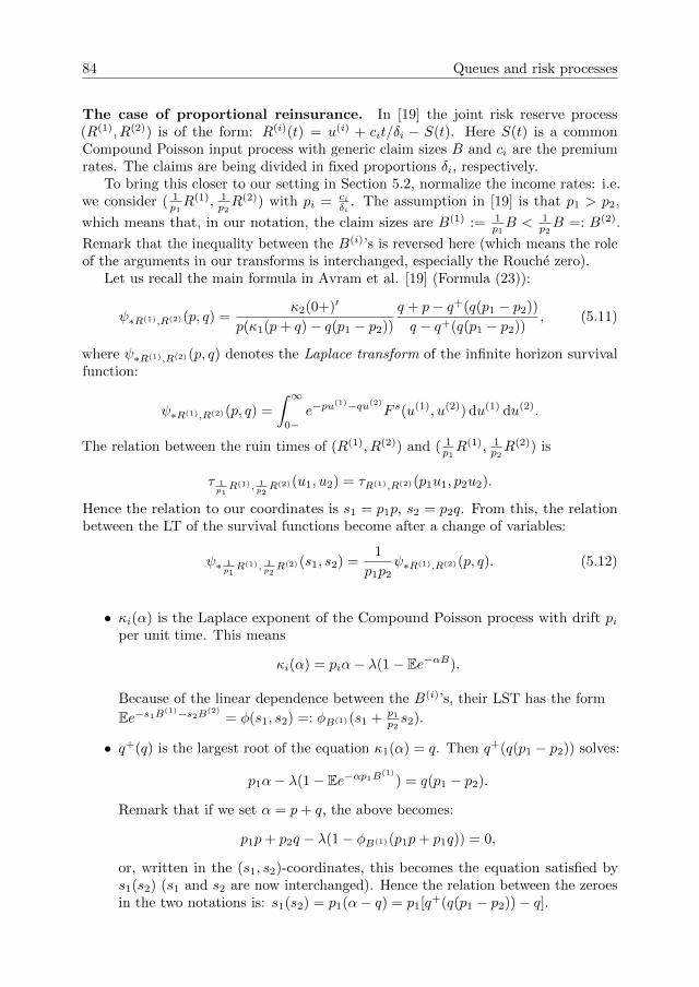
84 Queues and risk processes

The case of proportional reinsurance. In [19] the joint risk reserve process(R(1), R(2)) is of the form: R(i)(t) = u(i) + cit/δi − S(t). Here S(t) is a commonCompound Poisson input process with generic claim sizes B and ci are the premiumrates. The claims are being divided in fixed proportions δi, respectively.

To bring this closer to our setting in Section 5.2, normalize the income rates: i.e.we consider ( 1

p1R(1), 1

p2R(2)) with pi = ci

δi. The assumption in [19] is that p1 > p2,

which means that, in our notation, the claim sizes are B(1) := 1p1B < 1

p2B =: B(2).

Remark that the inequality between the B(i)’s is reversed here (which means the roleof the arguments in our transforms is interchanged, especially the Rouche zero).

Let us recall the main formula in Avram et al. [19] (Formula (23)):

ψ∗R(1),R(2)(p, q) =κ2(0+)′

p(κ1(p+ q)− q(p1 − p2))

q + p− q+(q(p1 − p2))

q − q+(q(p1 − p2)), (5.11)

where ψ∗R(1),R(2)(p, q) denotes the Laplace transform of the infinite horizon survivalfunction:

ψ∗R(1),R(2)(p, q) =

∫ ∞0−

e−pu(1)−qu(2)

F s(u(1), u(2)) du(1) du(2).

The relation between the ruin times of (R(1), R(2)) and ( 1p1R(1), 1

p2R(2)) is

τ 1p1R(1), 1

p2R(2)(u1, u2) = τR(1),R(2)(p1u1, p2u2).

Hence the relation to our coordinates is s1 = p1p, s2 = p2q. From this, the relationbetween the LT of the survival functions become after a change of variables:

ψ∗ 1p1R(1), 1

p2R(2)(s1, s2) =

1

p1p2ψ∗R(1),R(2)(p, q). (5.12)

• κi(α) is the Laplace exponent of the Compound Poisson process with drift piper unit time. This means

κi(α) = piα− λ(1− Ee−αB).

Because of the linear dependence between the B(i)’s, their LST has the form

Ee−s1B(1)−s2B(2)

= φ(s1, s2) =: φB(1)(s1 + p1p2s2).

• q+(q) is the largest root of the equation κ1(α) = q. Then q+(q(p1 − p2)) solves:

p1α− λ(1− Ee−αp1B(1)

) = q(p1 − p2).

Remark that if we set α = p+ q, the above becomes:

p1p+ p2q − λ(1− φB(1)(p1p+ p1q)) = 0,

or, written in the (s1, s2)-coordinates, this becomes the equation satisfied bys1(s2) (s1 and s2 are now interchanged). Hence the relation between the zeroesin the two notations is: s1(s2) = p1(α− q) = p1[q+(q(p1 − p2))− q].

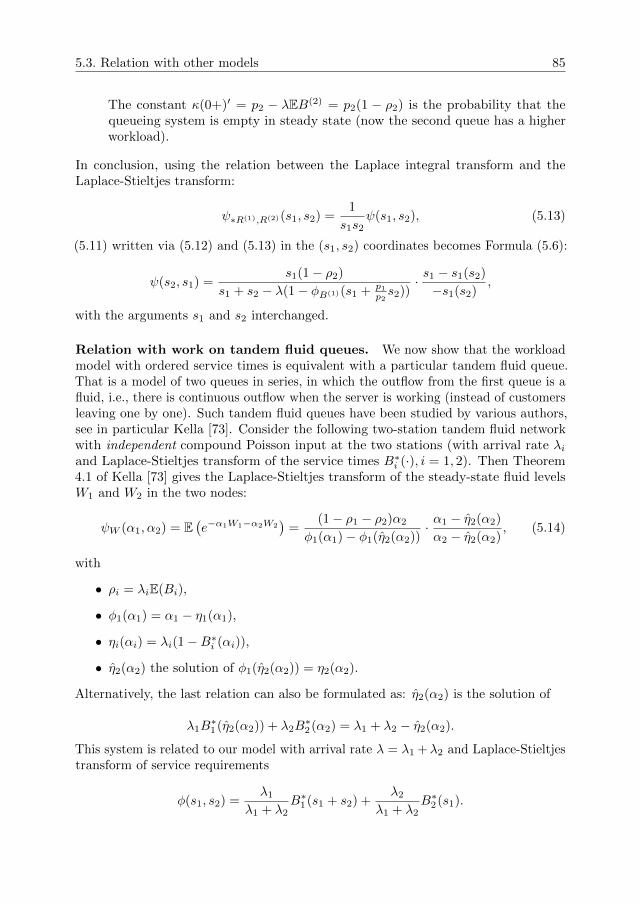
5.3. Relation with other models 85

The constant κ(0+)′ = p2 − λEB(2) = p2(1 − ρ2) is the probability that thequeueing system is empty in steady state (now the second queue has a higherworkload).

In conclusion, using the relation between the Laplace integral transform and theLaplace-Stieltjes transform:

ψ∗R(1),R(2)(s1, s2) =1

s1s2ψ(s1, s2), (5.13)

(5.11) written via (5.12) and (5.13) in the (s1, s2) coordinates becomes Formula (5.6):

ψ(s2, s1) =s1(1− ρ2)

s1 + s2 − λ(1− φB(1)(s1 + p1p2s2))

· s1 − s1(s2)

−s1(s2),

with the arguments s1 and s2 interchanged.

Relation with work on tandem fluid queues. We now show that the workloadmodel with ordered service times is equivalent with a particular tandem fluid queue.That is a model of two queues in series, in which the outflow from the first queue is afluid, i.e., there is continuous outflow when the server is working (instead of customersleaving one by one). Such tandem fluid queues have been studied by various authors,see in particular Kella [73]. Consider the following two-station tandem fluid networkwith independent compound Poisson input at the two stations (with arrival rate λiand Laplace-Stieltjes transform of the service times B∗i (·), i = 1, 2). Then Theorem4.1 of Kella [73] gives the Laplace-Stieltjes transform of the steady-state fluid levelsW1 and W2 in the two nodes:

ψW (α1, α2) = E(e−α1W1−α2W2

)=

(1− ρ1 − ρ2)α2

φ1(α1)− φ1(η2(α2))· α1 − η2(α2)

α2 − η2(α2), (5.14)

with

• ρi = λiE(Bi),

• φ1(α1) = α1 − η1(α1),

• ηi(αi) = λi(1−B∗i (αi)),

• η2(α2) the solution of φ1(η2(α2)) = η2(α2).

Alternatively, the last relation can also be formulated as: η2(α2) is the solution of

λ1B∗1(η2(α2)) + λ2B

∗2(α2) = λ1 + λ2 − η2(α2).

This system is related to our model with arrival rate λ = λ1 +λ2 and Laplace-Stieltjestransform of service requirements

φ(s1, s2) =λ1

λ1 + λ2B∗1(s1 + s2) +

λ2

λ1 + λ2B∗2(s1).

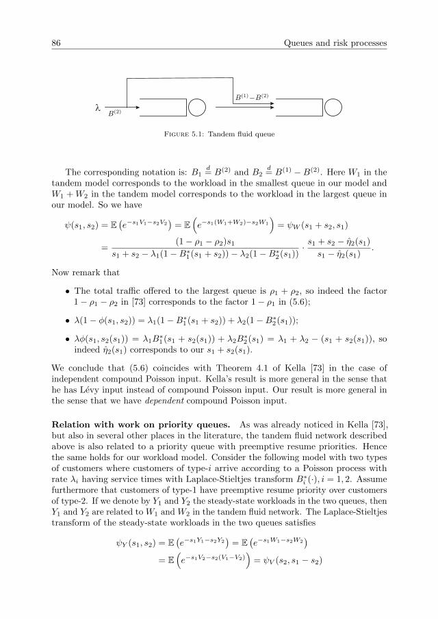
86 Queues and risk processes

lB(2)

B(1)−B(2)

1

Figure 5.1: Tandem fluid queue

The corresponding notation is: B1d= B(2) and B2

d= B(1) −B(2). Here W1 in the

tandem model corresponds to the workload in the smallest queue in our model andW1 +W2 in the tandem model corresponds to the workload in the largest queue inour model. So we have

ψ(s1, s2) = E(e−s1V1−s2V2

)= E

(e−s1(W1+W2)−s2W1

)= ψW (s1 + s2, s1)

=(1− ρ1 − ρ2)s1

s1 + s2 − λ1(1−B∗1(s1 + s2))− λ2(1−B∗2(s1))· s1 + s2 − η2(s1)

s1 − η2(s1).

Now remark that

• The total traffic offered to the largest queue is ρ1 + ρ2, so indeed the factor1− ρ1 − ρ2 in [73] corresponds to the factor 1− ρ1 in (5.6);

• λ(1− φ(s1, s2)) = λ1(1−B∗1(s1 + s2)) + λ2(1−B∗2(s1));

• λφ(s1, s2(s1)) = λ1B∗1(s1 + s2(s1)) + λ2B

∗2(s1) = λ1 + λ2 − (s1 + s2(s1)), so

indeed η2(s1) corresponds to our s1 + s2(s1).

We conclude that (5.6) coincides with Theorem 4.1 of Kella [73] in the case ofindependent compound Poisson input. Kella’s result is more general in the sense thathe has Levy input instead of compound Poisson input. Our result is more general inthe sense that we have dependent compound Poisson input.

Relation with work on priority queues. As was already noticed in Kella [73],but also in several other places in the literature, the tandem fluid network describedabove is also related to a priority queue with preemptive resume priorities. Hencethe same holds for our workload model. Consider the following model with two typesof customers where customers of type-i arrive according to a Poisson process withrate λi having service times with Laplace-Stieltjes transform B∗i (·), i = 1, 2. Assumefurthermore that customers of type-1 have preemptive resume priority over customersof type-2. If we denote by Y1 and Y2 the steady-state workloads in the two queues, thenY1 and Y2 are related to W1 and W2 in the tandem fluid network. The Laplace-Stieltjestransform of the steady-state workloads in the two queues satisfies

ψY (s1, s2) = E(e−s1Y1−s2Y2

)= E

(e−s1W1−s2W2

)= E

(e−s1V2−s2(V1−V2)

)= ψV (s2, s1 − s2)

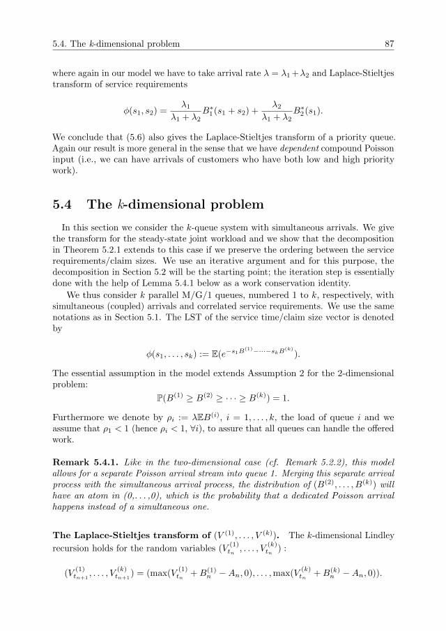
5.4. The k-dimensional problem 87

where again in our model we have to take arrival rate λ = λ1 +λ2 and Laplace-Stieltjestransform of service requirements

φ(s1, s2) =λ1

λ1 + λ2B∗1(s1 + s2) +

λ2

λ1 + λ2B∗2(s1).

We conclude that (5.6) also gives the Laplace-Stieltjes transform of a priority queue.Again our result is more general in the sense that we have dependent compound Poissoninput (i.e., we can have arrivals of customers who have both low and high prioritywork).

5.4 The k-dimensional problem

In this section we consider the k-queue system with simultaneous arrivals. We givethe transform for the steady-state joint workload and we show that the decompositionin Theorem 5.2.1 extends to this case if we preserve the ordering between the servicerequirements/claim sizes. We use an iterative argument and for this purpose, thedecomposition in Section 5.2 will be the starting point; the iteration step is essentiallydone with the help of Lemma 5.4.1 below as a work conservation identity.

We thus consider k parallel M/G/1 queues, numbered 1 to k, respectively, withsimultaneous (coupled) arrivals and correlated service requirements. We use the samenotations as in Section 5.1. The LST of the service time/claim size vector is denotedby

φ(s1, . . . , sk) := E(e−s1B(1)−···−skB(k)

).

The essential assumption in the model extends Assumption 2 for the 2-dimensionalproblem:

P(B(1) ≥ B(2) ≥ · · · ≥ B(k)) = 1.

Furthermore we denote by ρi := λEB(i), i = 1, . . . , k, the load of queue i and weassume that ρ1 < 1 (hence ρi < 1, ∀i), to assure that all queues can handle the offeredwork.

Remark 5.4.1. Like in the two-dimensional case (cf. Remark 5.2.2), this modelallows for a separate Poisson arrival stream into queue 1. Merging this separate arrivalprocess with the simultaneous arrival process, the distribution of (B(2), . . . , B(k)) willhave an atom in (0,. . . ,0), which is the probability that a dedicated Poisson arrivalhappens instead of a simultaneous one.

The Laplace-Stieltjes transform of (V (1), . . . , V (k)). The k-dimensional Lindley

recursion holds for the random variables (V(1)tn , . . . , V

(k)tn ) :

(V(1)tn+1

, . . . , V(k)tn+1

) = (max(V(1)tn +B(1)

n −An, 0), . . . ,max(V(k)tn +B(k)

n −An, 0)).

88 Queues and risk processes

For ψn(s1, . . . , sk) := E(e−s1V

(1)tn−...−skV (k)

tn

), n ≥ 1, the Lindley recursion gives

after straightforward calculations:

ψn+1(s1, . . . , sk) =

k∑j=1

λ

λ−∑ji=1 si

[φ(j)(s1, . . . , sj)ψ

(j)n (s1, . . . , sj)

− φ(j−1)(s1, . . . , sj−1)ψ(j−1)n (s1, . . . , sj−1)

]+ φ(0)ψ(0)

n (5.15)

where we used the following notation for simplicity: ψ(k)n (s1, . . . , sk) := ψn(s1, . . . , sk)

with ψ(0)n := ψn(λ, 0, . . . , 0), and

ψ(j)n (s1, . . . , sj) := ψn(s1, . . . , sj , λ−

j∑i=1

si, 0, . . . , 0︸ ︷︷ ︸k−j−1 arguments

), for 1 ≤ j ≤ k − 1.

φ(j)(s1, . . . , sj) is analogously defined for j = 0, . . . , k. By taking n→∞ in (5.15), weobtain for ψ(s1, . . . , sk) := limn→∞ ψn(s1, . . . , sk),(

1− λφ(s1,...,sk)

λ−∑ki=1 si

)ψ(s1, . . . , sk) =

k−1∑j=0

(λ

λ−∑ji=1 si

− λ

λ−∑j+1i=1 si

)· φ(j)(s1, . . . , sj)ψ

(j)(s1, . . . , sj), (5.16)

with ψ(j) := limn→∞

ψ(j)n ; and φ(0)ψ(0) = P(V (1) +B(1) ≤ A) = 1− ρ1.

Formula (5.16) has a simple recursive structure, and we can rewrite it as:

(1− λφ(s1,...,sk)

λ−∑ki=1 si

)ψ(s1, . . . , sk) =

(λ

λ−∑k−1i=1 si

− λλ−∑k

i=1 si

)φ(k−1)(s1, . . . , sk−1)·

ψ(k−1)(s1, . . . , sk−1) +(

1− λφ(s1,...,sk−1,0)

λ−∑k−1i=1 si

)ψ(s1, . . . , sk−1, 0).

(5.17)

Denote by Cj :=(

1− λφ(s1,...,sj ,0,...,0)

λ−∑ji=1 si

)ψ(s1, . . . , sj , 0, . . . , 0), and remark that

ψ(s1, . . . , sj , 0, . . . , 0) is the transform of the workload in the j-dimensional systemobtained by ignoring the last (k − j) queues, j = 1, . . . , k.

Proposition 5.4.1. The LST of the steady-state workload in the k ≥ 3 systems isgiven by:

ψ(s1, . . . , sk) =(1− ρk)(Sk − sk)∑k

i=1 si − λ(1− φ(s1, . . . , sk))

k−1∏j=2

1− ρj1− ρj+1

Sj − sjSj+1

· 1− ρ1

1− ρ2

s1

S2,

(5.18)with Sj = Sj(s1, ..., sj−1) the unique solution of the equation

λφ(s1, . . . , sj , 0, . . . , 0) = λ−j∑i=1

si,

5.4. The k-dimensional problem 89

with Re (s1 + · · ·+ sj−1 + Sj(s1, . . . , sj−1)) > 0, for all j = 2, . . . , k.

Proof. The key remark is that sk is not among the arguments of the functions ψ(j)

that appear in the righthand side of (5.16) or (5.17). Similarly as in Section 5.2,Rouche’s theorem (Lemma 5.6.1) applied to s1 replaced by s1 + · · · + sk−1 and s2

replaced by sk, yields the existence of a unique solution Sk = Sk(s1, . . . , sk−1) of theequation

λφ(s1, . . . , sk) = λ−k∑i=1

si,

such that Sk(s1, . . . , sk−1) +∑k−1i=1 si has positive real part. Hence the hyper-surface

given by Sk = Sk(s1, . . . , sk−1) is contained in the regularity domain of ψ(s1, . . . , sk),and then the righthand side of (5.17) must be zero. This gives the following relationfor ψ(k−1)(s1, . . . ,sk−1):

(φ(k−1) · ψ(k−1))(s1, . . . , sk−1) =(λ−∑k−1

i=1 si)φ(s1, . . . , sk−1, Sk)

SkCk−1.

By substituting back into Equation (5.17), we obtain the recursion

Ck =λ−∑k−1

i=1 si

λ−∑ki=1 si

· Sk − skSk

Ck−1

with initial condition C2 = −(1− ρ1) s1λ−s1−s2

S2−s2S2

, which follows from (5.6). Fromthis, we obtain (5.18), after rearranging the factors. The proof is complete.

Interpretation of the Rouche zero. It is worthwhile to change the coordinates:(s1, s2, . . . , sk)→ (s1, s2, . . . , sk−1,

∑ki=1 si). We can rewrite

φ(s1, . . . , sk) = Ee−s1(B(1)−B(k))−...−sk−1(B(k−1)−B(k))−(∑ki=1 si)B

(k)

Let us denote it by φ(s1, . . . , sk−1,∑ki=1 si). This is the transform of the extra

service time (relative to the shortest queue) in the first k − 1 queues, together withthe shortest one. It turns out there is a connection between Sk(s1, . . . , sk−1) and thejoint extra work in systems 1 to k − 1 at the end of a busy period in system k. Letus denote this extra work by (U1, U2, . . . , Uk−1), with LST U∗k (s1, . . . , sk−1), and letF (x1, x2, . . . , xk) be the c.d.f. of (B(1) − B(k), . . . , B(k−1) − B(k), B(k)). Then by asimilar argument as the one leading to (5.7), U∗k (s1, . . . , sk−1) satisfies the identity

U∗k (s1, . . . , sk−1) =

∫e−k−1∑i=1

sixi∞∑n=0

(λxk)n

n!e−λxk [U∗k (s1, . . . , sk−1)]nF (dx1 . . . dxk)

= φ(s1, . . . , sk−1, λ[1− U∗k (s1, . . . , sk−1)]). (5.19)

Comparing this with the identity for the Rouche zero,

λ− (s1 + · · ·+ sk−1 + Sk) = λφ(s1, . . . , sk−1, s1 + · · ·+ sk−1 + Sk),

90 Queues and risk processes

gives the relation analogous to (5.8):

λU∗k (s1, . . . , sk−1) = λ− (s1 + · · ·+ sk−1 + Sk), (5.20)

which follows because the Rouche zero is unique.Let us fix our attention on the case k = 3 for the moment. Then identity (5.18)

becomes

ψ(s1, s2, s3) =(1− ρ3)(S3 − s3)

s1 + s2 + s3 − λ[1− φ(s1, s2, s3)]· 1− ρ2

1− ρ3

S2 − s2

S3· 1− ρ1

1− ρ2

s1

S2. (5.21)

U(1),2

U(1),1

U(1),1

U(2),1 U(2),1

U(2),1U(2),1

V(1)

V(2)

V(3)

Ũ(1),2

U(1),1

U(1),1

Figure 5.2: Work in the original system (left) and in the virtual system (right)

Work conservation. We would like to give a probabilistic interpretation of (5.21).In order to achieve this, we start by considering the joint extra work in queues 1and 2 at the end of a busy period in queue 3. This has LST U∗3 (s1, s2) as inputin a 2-dimensional system with simultaneous Poisson arrivals, which is obtained bycontracting the busy cycles in queue 3. We call this the 2-dimensional virtual system.

5.4. The k-dimensional problem 91

Remark that the inter-arrival times in the virtual system are precisely the idle periodsin queue 3.

For this construction, the key observation is that the steady-state extra work in thevirtual queue 1 at the end of the busy period in the virtual queue 2 is the same as theextra work in the initial queue 1 at the end of the busy period in the original queue 2.In analytic form, let U∗2 (s1) be the LST of the extra work in the virtual system andU∗2 (s1) be the LST of the extra work in the original system, see Figure 5.2.

Lemma 5.4.1.U∗2 (s1) = U∗2 (s1).

Proof. We begin by remarking that the extra work (U (1),1, U (2),1) in the first 2 queuesat the end of a busy period in queue 3 satisfies the a.s. inequality U (1),1 ≥ U (2),1.Since this is the input in the virtual system, from Proposition 5.2.1, U∗2 (s1) satisfiesthe identity (5.7) with U∗3 (s1, s2) instead of φ(s1, s2):

U∗3 (s1, λ[1− U∗2 (s1)]− s1) = U∗2 (s1). (5.22)

At the same time, via (5.19), U∗3 (s1, s2) satisfies

φ(s1, s2, λ(1− U∗3 (s1, s2))− s1 − s2) = U∗3 (s1, s2).

If we substitute this fixed point identity in (5.22) above, we have

φ(s1, λ(1− U∗2 (s1))− s1, 0) = U∗2 (s1).

On the other hand, this is also the identity (5.7) satisfied by U∗2 (s1), in the 2-dimensionalsystem obtained by ignoring the last queue. Hence, from the uniqueness of Rouche’szero, U∗2 (s1) = U∗2 (s1) (See Figure 5.2). This completes the proof.We can rewrite (19) using (21):

ψ(s1, s2, s3) = (1− ρ3)s1 + s2 + s3 − λ(1− U∗3 (s1, s2))

s1 + s2 + s3 − λ(1− φ(s1, s2, s3))

· 1− ρ2

1− ρ3

s1 + s2 − λ(1− U∗2 (s1))

s1 + s2 − λ(1− U∗3 (s1, s2))· 1− ρ1

1− ρ2

s1

s1 − λ(1− U∗2 (s1)). (5.23)

Remark that the atom 1−ρ11−ρ2 above is the conditional probability that queue 1 is

empty, given that queue 2 is empty; and similarly for 1−ρ21−ρ3 . In addition, the last factor

in (5.23) is the Pollaczek-Khinchine representation for an M/G/1 queue with servicetimes having LST U∗2 (s1). Now we are ready to give the main result of this section.

Theorem 5.4.1. In steady state, the joint workload distribution decomposes as anindependent sum:

(V (1), V (2), V (3))d= (V (1),1, V (2),1, V (3)) + (V (1),2, V (2),2, 0) + (V (1),3, 0, 0).

The first term in the sum represents the steady-state distribution of the modified jointworkload process obtained by removing the extra work in the first two queues at the

92 Queues and risk processes

end of a busy period in the third queue. The second term is the workload in the firsttwo queues obtained by removing the extra work in the first queue at the end of a busycycle in the second queue. Finally the third term represents the workload in the virtualM/G/1 queue with input distributed as the extra work in queue 1, at the end of a busyperiod in queue 2.

Proof. Consider the modified work process that evolves in steady state as

(V (1),1, V (2),1, V (3))d=(V (1),1 +B(1) −A, V (2),1 +B(2) −A, V (3) +B(3) −A

),

if A < V (3) +B(3); and (V (1),1, V (2),1, V (3)) = (0, 0, 0), else.By similar computations as the ones leading to Formula (5.9), we obtain

ψ(s1, s2, s3) = (1− ρ3)s1 + s2 + s3 − λ(1− U∗3 (s1, s2))

s1 + s2 + s3 − λ(1− φ(s1, s2, s3)).

This is the first factor in (5.23). For the second one, consider the following modifiedvirtual workload process that evolves in steady state as

(V (1),2, V (2),2, 0)d=

(V (1),2 + U (1),1 −A, V (2),2 + U (2),1 −A, 0

),

if A < V (2),2 + U (2),1,(0, 0, 0), if A ≥ V (2),2 + U (2),1,

with (U (1),1, U (2),1) the extra work vector in the first two queues at the end of a busyperiod in queue 3. Here we remove the excess workload in the virtual queue 1 at theend of the busy period in the virtual queue 2, which by Lemma 5.4.1 is the same as inthe original system. In terms of LST’s , this becomes

ψ1(s1, s2) =1− ρ1

1− ρ2

s1 + s2 − λ(1− U∗2 (s1))

s1 + s2 − λ(1− U∗3 (s1, s2)).

Finally, the third factor in (5.23) is the Pollaczek-Khinchine representation of thesteady-state workload in the M/G/1 queue with service time distributed as the extrawork in queue 1 at the end of a busy period in queue 2. This completes the proof.

These considerations can be iterated now for the general k-dimensional system.

Corollary 5.4.1. The steady-state joint workload in the k systems decomposes intothe independent sum

(V (1), . . . , V (k))d= (V (1),1, . . . , V (k−1),1, V (k)) + (V (1),2, . . . , V (k−2),2, V (k−1),2, 0)

+ · · ·+ (V (1),k−1, V (2),k−1, 0, . . . , 0) + (V (1),k, 0, . . . , 0),

where the jth term in the sum satisfies the identity in distribution (j=2,. . . ,k):

(V (1),j ,V (2),j , . . . , V (k−j),j , V (k−j+1),j , 0, . . . , 0)d=(V (1),j + U (1),j−1 −A,

5.5. The general two-dimensional workload/reinsurance problem 93

V (2),j + U (2),j−1 −A, . . . , V (k−j+1),j −B(k−j+1) −A, 0, . . . , 0),

if A ≤ V (k−j+1),j −B(k−j+1),

and (0, . . . , 0) else. U (i),j is the extra workload in queue i at the end of a busy periodin queue (k − j + 1), for i > k − j + 1.

5.5 The general two-dimensional workload/reinsur-ance problem

In this section we consider the general two-dimensional workload problem: pairs ofcustomers arrive simultaneously at two parallel queues Q1 and Q2 according to a

Poisson(λ) process, the nth pair requiring service times (B(1)n , B

(2)n ) with LST φ(s1, s2).

We are interested in the steady-state workload vector (V (1), V (2)) with LST ψ(s1, s2).By the duality that is exposed in Section 2.2, ψ(s1, s2) is also the Laplace transform(w.r.t. u(1) and u(2)) of the probability that both portfolios of an insurance company

with simultaneous claims (B(1)n , B

(2)n ), with initial capital u(1) and u(2), will survive.

In Section 5.2 we have determined ψ(s1, s2) for the special case that P(B(1) ≥B(2)) = 1. We now show how the general case – B

(1)n and B

(2)n having an arbitrary

joint distribution – has been solved in the literature (with the solution of that specialcase emerging as a degenerate solution). We shall successively discuss the contributionsof Baccelli [21], De Klein [76] and Cohen [43], who have treated the two-dimensionalworkload problem with simultaneous arrivals in increasing generality. Starting point inall those three studies is the following functional equation for ψ(s1, s2), which is derivedby studying the 2-dimensional Markovian workload process during an infinitesimalamount of time ∆t:

K(s1, s2)ψ(s1, s2) = s2ψ1(s1) + s1ψ2(s2), Re s1, s2 ≥ 0. (5.24)

Here the so-called kernel K(s1, s2) is given by:

K(s1, s2) := s1 + s2 − λ(1− φ(s1, s2)), (5.25)

and

ψ1(s1) := E[e−s1V(1)

(V (2) = 0)], ψ2(s2) := E[e−s2V(2)

(V (1) = 0)], (5.26)

with (·) denoting an indicator function.

Remark 5.5.1. In the special case of Section 5.2, with P(B(1) ≥ B(2)) = 1, onehas ψ2(s2) ≡ P(V (1) = 0), because V (2) cannot be positive when V (1) = 0. It thenremains to find ψ1(s1). This is done by observing (cf. Appendix B) that, for all s1

with Re s1 > 0, there is a unique zero s2(s1) of the kernel, with Re s2(s1) > Re (−s1).This immediately yields that ψ1(s1) = − s1

s2(s1)P(V (1) = 0), which is readily seen to be

in agreement with (5.6).Equation (5.3), which was obtained by studying the workloads at arrival epochs

(i.e., the waiting times; by PASTA they have the same distribution as the steady-state

94 Queues and risk processes

workloads), looks slightly different from (5.24), but using (5.5) it is readily seen thatthey are equivalent.

Globally speaking, the essential steps in [21, 76, 43] are the following.Step 1: find a suitable set of zeroes (s1, s2), with Re s1 ≥ 0, Re s2 ≥ 0, of thekernel K(s1, s2), i.e., K(s1, s2) = 0. Because ψ(s1, s2) is regular for all (s1, s2) withRe s1, s2 ≥ 0, one must have for all these zeroes:

s2ψ1(s1) = −s1ψ2(s2). (5.27)

It is further observed that ψ1(s1) is regular for Re s1 > 0, continuous for Re s1 ≥ 0,and that ψ2(s2) is regular for Re s2 > 0, continuous for Re s2 ≥ 0.Step 2: formulate a boundary value problem for ψ1(s1) and ψ2(s2). There are varioustypes of boundary value problems, like the Riemann and the Wiener-Hopf boundaryvalue problems. Typically, they ask to determine two functions P1(·) and P2(·), whichsatisfy a relation on a particular boundary B, while P1(·) is regular in the interior B+

and P2(·) is regular in the exterior B−. B could be the unit circle (Riemann boundaryvalue problem), or the imaginary axis (Wiener-Hopf boundary value problem; B+ nowis the left-half plane). We refer to Gakhov [65] and Mushkelishvili [87] for excellentexpositions of such boundary value problems and their variants, like the boundaryvalue problem with a shift. The latter occurs in the approach of De Klein [76], seebelow.Step 3: solve the boundary value problem for ψ1(·) and ψ2(·) with boundary B. If B isa smooth closed contour that is not a circle, the use of a conformal mapping from Bto the unit circle C is required to arrive at a Riemann boundary value problem forthe unit circle, the solution of which can be found in [65, 87]. Thus one obtains ψ1(s1)and ψ2(s2) inside certain regions; subsequently, one may use analytic continuation tofind them in Re s1, s2 ≥ 0. Finally, ψ(s1, s2) follows from (5.24).

Remark 5.5.2. Application of the boundary value method in queueing theory waspioneered by Fayolle and Iasnogorodski in [55]. They used this method to analyzethe joint queue length process in two coupled processors, viz., two M/M/1 queueswhich operate at unit speeds when the other queue is not empty, but at different speedswhen the other queue is empty. The method was subsequently developed in [41] fora large class of two-dimensional random walks; various queueing applications werealso discussed in [41]. See [42] for a survey of the method in queueing theory, and see[56, 43] for two monographs which have further developed the theory of two-dimensionalrandom walks. Part IV of [43] explores the analysis of k-dimensional random walkswith k > 2. Results for k > 2 are very limited, and it seems fair to conclude that theboundary value method is, apart from a few special cases, restricted to two-dimensionalrandom walks.

Remark 5.5.3. We strongly believe that the boundary value method also has a largepotential in the analysis of two-dimensional risk models. Due to the duality between thereinsurance model and the 2-queue model with simultaneous arrivals, the publicationsof Baccelli [21], DeKlein [76], Cohen [43] are of immediate relevance to the reinsuranceproblem. These publications seem unknown in the insurance community (see, e.g.,Chan et al. [37], who pose the two-dimensional risk problem and stop at Equation

5.5. The general two-dimensional workload/reinsurance problem 95

(5.24) (where [21, 76, 43] begin). They have remained largely unnoticed even in thequeueing community, perhaps because of their complexity and because [21] and [76]did not appear in the open literature. For these reasons, we now successively exposethe approaches in [21], [76] and [43] at some length.

The approach of Baccelli [21]Baccelli [21] restricts himself to the case of exchangeable (B(1), B(2)), i.e., P(B(1) <x,B(2) < y) = P(B(1) < y,B(2) < x), or equivalently, φ(s1, s2) = φ(s2, s1). We brieflyreview the three steps mentioned above.Step 1 in [21] is as follows. Consider zero pairs (s1, s2) = (g + iu, g − iu) of kernelK(s1, s2), with u ∈ R and with g = g(u) the unique zero in Re g ≥ 0 of

2g = λ(1− φ(g + iu, g − iu)).

Using the exchangeability, it can be shown that this unique zero is real and non-negative, while g(−u) = g(u), u ∈ R.Step 2. Consider the arc A = {s1 : s1 = g(u) + iu, u ∈ R}, with g(u) the zerodefined above. This is a smooth arc, located in the right half-plane. Baccelli finds aconformal mapping p(·) of the interior C+ of the unit circle C onto A+, the ‘interior’of A located on the right of A, and a conformal mapping q(·) of C−, the exterior ofthe unit circle, onto A+; their limits on C are denoted by p+(z) and q−(z), whichare each other’s complex conjugates because of the exchangeability. Noticing thatp+(−1) = q−(−1) = 0, he multiplies both sides of (5.27) with 1+z. This yields (divideboth sides of (5.27) by s1s2):

(1 + z)ψ1(p+(z))

p+(z)= −(1 + z)

ψ2(q−(z))

q−(z), |z| = 1. (5.28)

Because of the regularity properties of the conformal mappings and of ψ1(s1) andψ2(s2), Re s1, s2 > 0, one now arrives at a simple boundary value problem: we have(5.28) for |z| = 1, while the left-hand side of (5.28) is regular for |z| < 1, and theright-hand side is regular for |z| > 1.Step 3. The solution of this problem immediately follows from Liouville’s theorem, cf.[102] p. 85:

ψ1(p(z)) =γ + δz

1 + zp(z), |z| < 1, ψ2(q(z)) =

γ + δz

1 + zq(z), |z| > 1.

Baccelli [21] shows that γ = −δ, and determines the remaining unknown constantδ by normalization. Having thus determined ψ1(s1) for s1 ∈ A+, he uses analyticcontinuation to obtain ψ1(s1) in the whole right half-plane; similarly for ψ2(s2). Finally,substitution in (5.24) determines ψ(s1, s2).

The approach of De Klein [76]De Klein [76], pp. 119-168, studies the general case of an arbitrary joint distributionof B(1) and B(2).Step 1 in [76] is as follows. He considers the same zero pairs as Baccelli (also suggestinganother set of zero pairs on p. 132). g(u) is no longer necessarily real, but for all realu there still is a unique zero g(u).

96 Queues and risk processes

Step 2. De Klein subsequently considers the simple, smooth arcs A1 = {s1 : s1 =g(u) + iu, u ∈ R} and A2 = {s2 : s2 = g(u) − iu, u ∈ R} in the right half-plane.Notice that A1 and A2 are each other’s complex conjugates in the exchangeable caseof Baccelli, but not in De Klein’s more general case. De Klein now uses the (unique)one-to-one mapping s2 = ω2(s1) from A1 onto A2 (with inverse ω1(s2)) determined bythe fact that, ∀s1 ∈ A1, (s1, ω2(s1)) is a zero pair of the kernel. Similarly, ∀s2 ∈ A2,(ω1(s2), s2) is a zero pair. Hence the following must hold:

ψ1(ω1(s2)) = −ω1(s2)

s2ψ2(s2), s2 ∈ A2. (5.29)

In addition, one has the regularity properties of the functions ψ1(·) and ψ2(·) whichwere listed below (5.27). Determination of functions ψ1(·) and ψ2(·) with theseregularity properties and satisfying (5.29) is a so-called shift problem, a boundaryvalue problem with a shift (cf. Sections 17 and 18 of [65]).Step 3. Gakhov [65] mentions two methods to solve such problems: (i) reduce theproblem to a Fredholm integral equation of the second kind, and (ii) reduce theproblem to an ordinary Riemann boundary value problem, by means of conformalmappings. De Klein [76] explores the first method in Section II.4.2 and the secondin Section II.4.3. We concentrate on the first method. De Klein first translates theshift problem to one on a finite smooth closed contour, via the conformal mappingζ(z) = 1−z

1+z (with inverse z(ζ) = 1−ζ1+ζ ) that maps Ai onto smooth closed contours Ti,

i = 1, 2; he then applies Gakhov’s first method. He obtains the following Fredholmintegral equation of the second kind for an unknown function G1(·) – which up to aconstant equals log{ψ1(z(·))}:

G1(p1) =1

2πi

∫T1

G1(v1)[1

v1 − p1− ν′2(v1)

ν2(v1)− ν2(p1)− 1

v1 − c1]dv1 +H1(p1), p1 ∈ T1,

(5.30)with H1(·) some known function, c1 some point in the interior of T1, and for ν2(v1)= ζ(ω2(z(v1))), v1 ∈ T1. After having solved the integral equation (which can be donenumerically in an efficient way, as shown by De Klein), one obtains ψ1(s1) for s1 ∈ T1,and then ψ2(s2) for s2 ∈ T2 via (5.27). The regularity of ψ1(s1) in the interior T+

1

subsequently allows one to obtain ψ1(s1), s1 ∈ T+1 , as a Cauchy integral; similarly for

ψ2(s2), s2 ∈ T+2 . By analytic continuation, ψ1(s1) and ψ2(s2) are then also uniquely

determined in Re s1 ≥ 0 and Re s2 ≥ 0, respectively. Finally, ψ(s1, s2) again followsfrom (5.24).

De Klein also explores Gakhov’s second method to treat the shift problem. However,this reduction to a Riemann boundary value problem requires a conformal mappingthat itself must be determined by solving another Fredholm integral equation of thesecond kind. In Chapter II.6 he extensively investigates the numerical solution of bothintegral equations by means of the Nystrom or quadrature method. He obtains, a.o.,accurate results for the mean sojourn time of a customer pair, viz., the time until bothcustomers of a pair have left the system.

The approach of Cohen [43]Cohen [43], Part III, considers a very general class of two-dimensional workload

processes. Basically, he combines the model with simultaneous arrivals and the coupled

5.6. Appendix B 97

processors model. The two servers have speeds r1 and r2 if they are both non-idle,and speeds r(1) and r(2) when the other server is idle. Furthermore, he also allows thepossibility of different joint service requirement distributions if a customer pair arriveswhen at least one of the servers is idle. Finally, he explicitly allows single arrivalsnext to simultaneous arrivals (cf. also [23]). Much of Part III of [43] is devoted to adetailed study of the ergodicity conditions and of the so-called hitting point processand hitting point identity of the workload process, hitting point referring to the firstentrance point of one of the axes.

In Chapter III.4 he determines the steady-state joint workload distribution fora variety of cases. For us, the most relevant cases are treated in Sections III.4.9and III.4.10. Section III.4.9 treats the model of De Klein [76]. The same zeropairs are used (Step 1), and the same smooth closed contours T1 and T2; Cohensubsequently uses Gakhov’s second method to arrive at a Riemann boundary valueproblem (Step 2). That boundary value problem actually is so simple that it can besolved straightforwardly by applying Liouville’s theorem, cf. Baccelli’s method above(Step 3); however, a conformal mapping is required, which is obtained as the solutionof another Fredholm integral equation of the second kind. A nice feature in SectionIII.4.9 is that ψ1(s) and ψ2(t), after normalization, are expressed as LST’s of waitingtime or workload distributions of special M/G/1 queues (which are related to hittingpoints).

Section III.4.10 treats the model of De Klein with the additional feature that thereis coupling of the servers, of a rather special form: r1

r(1)+ r2

r(2)= 1. This does not

change the kernel K(s, t) (which only refers to the interior of the state space, withboth servers active), so the same zero pairs and contours can still be used. However,it does change the right-hand side of (5.24), and hence a slightly different Riemannboundary value problem must be solved.

Remark 5.5.4. It should be observed that Baccelli [21], De Klein [76] and Cohen[43] all also solve the more complicated transient problem, of determining the jointtime-dependent distribution of the two workloads.

5.6 Appendix B

Lemma 5.6.1 (Rouche zero). For every s1 with Re s1 > 0 there exists a uniques2 = s2(s1) with Re s2(s1) > Re (−s1), that satisfies the identity

λφ(s1, s2) = λ− (s1 + s2).

Moreover the function: s1 → s2(s1) is analytic in Re s1 > 0.

Proof. For fixed s1 with Re s1 > 0, let f(s1 + s2) := λ− (s1 + s2). Consider in theright half-plane the contour C made up from the semicircle with center at −s1 andradius R > 2λ together with the line segment I := {−s1 + iw|w ∈ [−R,R]}. We showthat on this contour |λφ(s1, s2)| < |f(s1 + s2)|. We can bound |φ(s1, s2)| by

λ |φ(s1, s2)| = λ|φ(s1, s1 + s2)| ≤ λEe−Re s1(B(1)−B(2))−Re (s2+s1)B(2)

< λ.

98 Queues and risk processes

This holds everywhere in the domain of φ(s1, s2) if B(1) −B(2) has positive mass on(0,∞).

Now we bound |f(s1 + s2)|. When (s1 + s2) is on the semicircle (i.e |s1 + s2| = R >2λ), apply the triangle inequality to the triangle with vertices at 0, λ, s1 + s2, to find|λ−s1−s2| > λ. When (s1 +s2) ∈ I, by a similar argument we obtain |λ−s1−s2| ≥ λ,with equality only when s1 + s2 = 0. Hence on the contour C, |f(s1 + s2)| ≥ λ. Wecan now use Rouche’s theorem to conclude that the equation λφ(s1, s2) = λ− (s1 + s2)has a unique solution s2(s1) inside C, because the polynomial f(s1 + s2) has only onezero inside C, at λ. Letting R→∞, proves the assertion.

Chapter 6

Two parallel insurance lineswith simultaneous arrivals

As mentioned in the introductory Section 1.2, in the existing risk and insuranceliterature, there are not many approaches towards analyzing multidimensional models.

The approach we take in this chapter combines ideas from Chapters 3 and 5. InSection 6.2 we derive a functional equation for the survival function related to a2-dimensional risk reserve process, but unlike in Chapter 5, we do not assume thatthe claim intervals are exponentially distributed. A semi-Markov structure is assumedfor the arrival process which is in many respects a two-dimensional (vector-valued)version of the BMAP structure of Chapter 3. To be more precise, we assume the claimsize vector to be correlated with the time elapsed since the previous arrival. Such acorrelation is quite natural; e.g., a claim event that generates very large claims couldbe subjected to additional administrative/regulatory delays. The type of correlationbetween the inter-arrival time and the vector of claim sizes is an extension to twodimensions of the dependence structure studied in Chapter 3 for the generalized Sparre-Andersen model. It involves making a rationality assumption regarding the trivariateLST of inter-arrival time and claim size vector (Assumption 6.1.1), which extendsthe case where the vector with the aforementioned components has a multivariatephase type distribution (MPH). In addition, we also make the assumption that theclaim sizes are a.s. ordered (Assumption 6.1.2). Under these assumptions, we obtainour main result: An explicit expression for the (LST of the) two-dimensional survivalfunction, for a large class of vectors of interclaim times and claim amounts of bothrisk reserves. For example, this is the case if we consider proportional reinsurance.

The chapter is organized in the following way. In Section 6.1 we describe the modelin detail and present the main assumptions we will be working with.

For a start, an essential ingredient is the multivariate duality relation from Theorem2.2.1. This relation makes it clear that determining the survival function is equivalentto determining the two-dimensional waiting time distribution in a dual two-queuetwo-server queueing model with simultaneous arrivals of customers at both queues.With the help of the embedded random walk/queueing process we derive, in Section6.2, a stochastic recursion for the LST of the finite horizon survival function. In Section

99

100 Parallel insurance lines

6.3 we resolve the stationary version of this stochastic recursion, (6.8). The key toolused is a one-parameter Wiener-Hopf factorization of the bivariate kernel appearing in(6.8). More precisely, the Wiener-Hopf factors will depend on one parameter, which isthe first argument of that bivariate kernel; see Proposition 6.3.1 in Section 6.3. Themain result, Theorem 6.3.1, gives the LST of the survival function, or equivalentlythe stationary distribution of the waiting time/reflected random walk inside the non-negative quadrant (see also Theorem 2.2.1). In Section 6.4, we give an asymptoticdecomposition result for the joint LST of the waiting time, which can be written asa product, with one of the factors being the transform of the waiting time in thefirst queue conditional that the other queue is empty. This is an extension of thedecomposition result obtained in (5.10), Chapter 5.

In Section 6.5 we explain how to calculate the transform obtained in Theorem6.3.1 for some examples, and we numerically calculate the ruin functions/waitingtime distributions using an efficient inversion algorithm of den Iseger [70] - which isabout using the Gauss quadrature method to discretize the LST and then apply theinversion scheme of Abate and Whitt [1]. Finally, we also point out that the numericalresults suggest that the ruin functions appear to be stochastically ordered for varioustypes of correlations between inter-arrival times and claim sizes, a positive correlationapparently leading to smaller ruin probabilities.

6.1 Model description

Let us begin with the general assumptions on the two risk reserves. These are startedwith non-negative initial capital (u(1), u(2)); as long as there are no arrivals, thesurplus levels increase linearly with positive rates (c1, c2). At the nth claim arrival

epoch, claim sizes B(1)n and B

(2)n are respectively requested from each component.

The time between the (n − 1)th and nth claim arrival is denoted by An. The

sequence {(An, B(1)n , B

(2)n )}n≥1, is assumed to be an i.i.d. sequence, but within a triple,

(An, B(1)n , B

(2)n ) are allowed to be correlated. We will use A, B(1), B(2) respectively

for the generic inter-arrival time and claim sizes. In the above-described very generalset-up, the following assumption will allow us to explicitly determine the ruin/survivalprobabilities by using Wiener-Hopf factorization:

Assumption 6.1.1 (On the joint transform of A, B(1), B(2)). The triple trans-form

H(q0, q1, q2) := Ee−q0A−q1B(1)−q2B(2)

(6.1)

is a rational function in qi, i.e. it has representation G(q0,q1,q2)L(q0,q1,q2) such that G(q0, q1, q2)

and L(q0, q1, q2) are polynomials in the variables qi, i = 0, 1, 2.

G(q0, q1, q2) and L(q0, q1, q2) must satisfy some conditions, because their ratio is atransform, such as,

lim|q0|→∞,Re q0>0

H(q0, q1, q2) = E[e−q1B(1)−q2B(2)

1{A=0}].

6.1. Model description 101

We can assume without loss of generality that A > 0 a.s. Because of the abovelimit, this means the degree of G as a polynomial in q0, Gq1,q2(q0), is strictly less thanthe degree of L as a polynomial in q0: Lq1,q2(q0), for all q1 and q2.

Remark 6.1.1. The class of rational multivariate Laplace-Stieltjes transforms containsthe class of LSTs of multivariate Phase-Type distributions (MPH); see Bladt andNielsen [29], where the rational transform class is called multivariate matrix-exponential(MME). All of the well-known classes of multivariate Phase-Type distributions areMME. Actually, all the examples we will present are MPH distributions with a specificcorrelation structure which are a special case of Kulkarni’s MPH* class [79]. There isno point in restricting ourselves to any of these subclasses. We will fully exploit thealgebraic representation of rational functions in order to derive explicitly the transformsof the two-dimensional survival/ruin functions.

The risk reserve process Rt = (R(1)t , R

(2)t ) is defined in (2.10). The associated types

of survival measures and the related ruin functions are defined in Section 2.2. Thischapter is mainly concerned with measuring the event that both risk reserve processessurvive indefinitely, i.e., we aim to determine the survival function F s(u(1), u(2)), orequivalently, the ruin function τ∧(u(1), u(2)), as defined by (2.11).

In this model, the two reserves are correlated due to simultaneous claim arrivalsand due to correlations that may exist in the claim size vector (B(1), B(2)).

From this point on we scale the risk reserve process by the income rates in eachcomponent (see Remark 5.2.1). The main idea is to exploit the fact that the embeddedprocess at arrival epochs of claims is a random walk in the plane with increments

(An−B(1)n /c1, An−B(2)

n /c2), conditioned on starting at (u(1), u(2)). The different waysin which the risk reserve process can be ruined correspond to the possible positions ofthe random walk

Rtn+1:= u−

n∑i=1

Xi, Xn = (B(1)n /c1 −An, B(2)

n /c2 −An), (6.2)

at the time of exit from the non-negative quadrant.This is a difficult model to analyze in full generality; in particular, it is more general

than the two-dimensional ruin process described in Chan et al. [37] and in Chapter 5.However, in the case that the claims in the first insurance line are larger than those inthe second, we are able to determine the two-dimensional survival function.

Assumption 6.1.2 (Ordering assumption). For a generic claim event (B(1), B(2)):

B(1)/c1 ≥ B(2)/c2 a.s. (6.3)

A special, important example for this ordering assumption is the case when there isa single arrival process such that the common claim is partitioned into fixed proportions(α, 1 − α), and we can always take w.l.o.g. α ∈ [1/2, 1] (α may even be a randomvariable with this interval as support). This special case then significantly generalizesthe setting in Avram et al. [19], where it is assumed that the common arrival process

102 Parallel insurance lines

is compound Poisson (and in particular the inter-arrival times are independent of theclaim sizes).

One can go a step further and assume there is a dedicated renewal-arrival streamof claims into the line which pays the greater share, say α. This is in line with theassumption in Badescu et al. [23] of a dedicated Poissonian stream of claims, andextends it, once we combine it with Assumption 6.1.1. Clearly this is not a proportionalreinsurance problem anymore. From a mathematical perspective, the analysis is moreinsightful than if one would just assume proportionality.

We take the following approach: using the duality arguments (Section 2.2), wederive a recursive equation for the survival function (Section 6.2). Using complexfunction theory, and under Assumptions 6.1.1 and 6.1.2, we solve the functionalequation that corresponds to the stochastic recursion in terms of survival functionLSTs (Section 6.3).

6.2 A functional equation

In this section we will consider the Laplace-Stieltjes transform of the survival functionF sn(u(1),u(2)). Theorem 2.2.1 and the usual relation between the waiting time vectorand the embedded workload vector Wn = Vtn (we assumed unit income/service rates,see Remark 5.2.1) implies that this equals the transform of the bivariate waiting timefor the nth customer:

Ee−s1W(1)n −s2W (2)

n =

∫e−s1u

(1)−s2u(2)

dF sn(u(1), u(2)), Re si ≥ 0, i = 1, 2. (6.4)

Our main goal in this section is to obtain a recursion between the LSTs of

(W(1)n+1,W

(2)n+1) and (W

(1)n ,W

(2)n ) using Lindley’s recursion (2.9). But first we point

out a sample-path relation between the risk reserve process and the reflected randomwalk which will be useful in the next section (the relation in Theorem 2.2.1 holds indistribution only). The event that any of the risk reserves is running at the maximumis the same as the event that the corresponding component of the reflected randomwalk is at 0.

Lemma 6.2.1. For Sn =∑ni=1Xi, n ≥ 1, it holds

{W (i)n+1 = 0} = {R(i)

tn+1= u(i) + max(0,−S(i)

1 , ...,−S(i)n )}, i = 1, 2.

Proof. R(i)tn+1

= u(i) − S(i)n and notice the following equivalence:

S(i)n −min(0, S

(i)1 , . . . , S(i)

n ) = 0⇔ −S(i)n = max(0,−S(i)

1 , . . . ,−S(i)n ).

The statement now follows from Proposition 2.2.1.

Remark 6.2.1. The event {W (i)n = 0} does not depend on the initial capital. The

event on the RHS in Lemma 6.2.1 above does not restrict the risk reserve process to

staying above 0; equivalently W(i)n on the LHS is not restricted to staying below level

u(i). This is in line with (2.13) in Theorem 2.2.1.

6.2. A functional equation 103

Below we point out how one can obtain a recursive equation for the LST of thesurvival function F sn(u(1), u(2)) in the general case without the ordering assumption.In Section 6.3 we solve this equation for the case when the risks are ordered. TheLindley recursion (2.9) becomes in terms of LSTs:

Ee−s1W(1)n+1−s2W

(2)n+1 = Ee−s1(W (1)

n +X(1)n )+−s2(W (2)

n +X(2)n )+ ,

with (x)+ = max(x, 0). Hence, with 1{E} the indicator function of event E,

Ee−s1W(1)n+1−s2W

(2)n+1 =E

[e−s1(W (1)

n +X(1)n )−s2(W (2)

n +X(2)n )1{−X(1)

n <W(1)n ,−X(2)

n <W(2)n }

]+ E

[e−s1(W (1)

n +X(1)n )1{−X(1)

n <W(1)n ,−X(2)

n ≥W (2)n }

]+ E

[e−s2(W (2)

n +X(2)n )1{−X(1)

n ≥W (1)n ,−X(2)

n <W(2)n }

]+ P(−X(1)

n ≥W (1)n ,−X(2)

n ≥W (2)n ). (6.5)

In view of (6.4), the left-hand side of (6.5) represents the LST of the survivalmeasure F sn+1. Below we also interpret each of the four terms in the righthand side interms of transforms of survival measures.Term 1: In terms of excursions away from the maximum of the surplus process (Lemma6.2.1), the first term on the RHS represents the transform of the survival measure inthe event that both risk reserves are during an excursion below the running maximumat time tn+1,

Ee−s1W(1)n+1−s2W

(2)n+11{W (1)

n+1>0,W(2)n+1>0} =∫

e−s1u(1)−s2u(2)

1{Rtn+1<

∨k=0,...,n

Rtk}dFsn+1(u(1), u(2)).

Above we used that on the event {W (i)n+1 > 0}, it holds that W

(i)n +X

(i)n = W

(i)n+1.

Terms 2 and 3: These can be translated in terms of survival functions using (6.4)again:

Ee−s1W(1)n+11{W (1)

n+1>0,W(2)n+1=0} =

∞∫0+

e−s1u(1)

1{R(1)tn+1

< maxk=0,...,n

R(1)tk

;R(2)tn+1

≥ maxk=0,...,n

R(2)tk}dF

sn+1(u(1), 0),

Ee−s2W(2)n+11{W (1)

n+1=0,W(2)n+1>0} =

∞∫0+

e−s2u(2)

1{R(1)tn+1

≥ maxk=0,...,n

R(1)tk

;R(2)tn+1

< maxk=0,...,n

R(2)tk}dF

sn+1(0, u(2)),

104 Parallel insurance lines

are ’boundary’ transforms. The survival measure that corresponds to F sn can havepositive mass on the axes of the non-negative quadrant, if nowhere else, at leastF sn(0, 0) = P(Wn = 0 |W0 = 0) is positive, i.e., it has an atom in the origin.Term 4: This is the probability that both risk reserves are surviving and running at amaximum, which by Lemma 6.2.1 and Theorem 2.2.1 is F sn+1(0, 0).

From an analytic point of view it is more convenient to rewrite (6.5) as a recursion.After adding and subtracting appropriate terms, one obtains,

Ee−s1W(1)n+1−s2W

(2)n+1 =

Ee−s1X(1)n −s2X(2)

n Ee−s1W(1)n −s2W (2)

n

+ E{e−s1(W (1)

n +X(1)n )[1− e−s2(W (2)

n +X(2)n )]1{W (1)

n+1>0,W(2)n+1=0}

}+ E

{e−s2(W (2)

n +X(2)n )[1− e−s1(W (1)

n +X(1)n )]1{W (1)

n+1=0,W(2)n+1>0}

}+ E

{[1− e−s1(W (1)

n +X(1)n )−s2(W (2)

n +X(2)n )]1{W (1)

n+1=0,W(2)n+1=0}

}.

(6.6)

Above we used that the increment Xn is independent of Wn. Under the assumptionthat the vector Wn has a limit in distribution, W , as n→∞, (6.6) becomes

K(s1, s2)Ee−s1W(1)−s2W (2)

=

E{e−s1(W (1)+X(1))[1−e−s2(W (2)+X(2))]1{W (1)>−X(1),W (2)≤−X(2)}

}+ E

{e−s2(W (2)+X(2))[1−e−s1(W (1)+X(1))]1{W (1)≤−X(1),W (2)>−X(2)}

}+ E

{[1−e−s1(W (1)+X(1))−s2(W (2)+X(2))]1{W (1)≤−X(1),W (2)≤−X(2)}

}, (6.7)

with ”kernel” K(s1, s2) := 1− Ee−s1X(1)−s2X(2)

and Re si = 0, i = 1, 2.

Remark 6.2.2. From Lemma 2.2.1, W has the same distribution as the all-timesupremum M := lim

n→∞Mn; and Mn being a sequence of non-decreasing random vectors

w.r.t. the componentwise order ’≤’, the limit always exists a.s., although it may havea defective distribution. In the next section we give a sufficient condition for M tohave a proper distribution under the assumption that risks are ordered.

6.3 Wiener-Hopf analysis of the stochastic recur-sion

In this section we resolve the functional equation (6.7) under the Assumptions 6.1.1and 6.1.2, i.e., we find the LST of the infinite horizon survival function:

F s = limn→∞

F sn,

6.3. Wiener-Hopf analysis of the stochastic recursion 105

the limit being considered in distribution. Theorem 2.2.1 together with a limitargument shows that this weak limit is the same as the c.d.f. of the stationary versionof the waiting time process (Wn)n≥0.

The section is divided into three subsections. Subsection 6.3.1 prepares theground, by making a key observation about the functional equation (6.7), introducingsome notation and discussing the stability condition. Subsection 6.3.2 expresses thetwo-dimensional LST ψ(s1, s2) of F s in a one-dimensional unknown function C(s1)(Proposition 6.3.1). That function is determined in Subsection 6.3.3, yielding our mainresult: Theorem 6.3.1.

6.3.1 Preparations

Introduce the extra claim amount δn := B(1)n /c1 −B(2)

n /c2 = X(1)n −X(2)

n , so that the

increments of the random walk Sn can be represented as Xn = (X(2)n + δn, X

(2)n ).

We first make the following key observation: The ordering assumption (6.3) implies

that when R(1)tn is at a maximum, necessarily R

(2)tn is at a maximum. Via Lemma 6.2.1,

this corresponds to the fact that the events

{W (1)n ≤ −X(1)

n , W (2)n > −X(2)

n } = {W (1)n+1 = 0,W

(2)n+1 > 0}

are null for all n ≥ 0. This means that the third term on the RHS of (6.6) is null andhence the second term on the RHS of (6.7) vanishes as well, so that after regroupingterms, (6.7) can be rewritten as

K(s1, s2)ψ(s1, s2) = −ψ1(s1, s2) + ψ2(s1) + P(W (1) +X(1) ≤ 0), (6.8)

where

ψ1(s1, s2) = Ee−s1(W (1)+X(2)+δ)−s2(W (2)+X(2))1{−X(2)≥W (2)},

ψ2(s1) = Ee−s1(W (1)+X(2)+δ)1{W (1)+δ>−X(2)≥W (2)}.

Consider the following function:

K(s1, z) := 1− Ee−s1δ−zX(2)

, Re s1 ≥ 0, Re z = 0.

This is related to K(s1, s2) that appears in (6.7) through the change of coordinates:K(s1, z) = K(s1, z − s1). In addition, remark that for fixed z, K(s1, z) is indeedanalytic in Re s1 > 0 because δ ≥ 0 a.s. Now let us change the coordinates: (s1, s2)→(s1, s1 + s2) =: (s1, z). Denote ψ(s1, z) := ψ(s1, z − s1), and similarly for ψ1(s1, z) :=ψ1(s1, z − s1). Then ψ1(s1, s2) becomes

ψ1(s1, s2) = E[e−s1(W (1)−W (2)+δ)−z(W (2)+X(2))1{−X(2)≥W (2)}

]=: ψ1(s1, z),

and therefore (6.8) can be rewritten as

K(s1, z)ψ(s1, z) = −ψ1(s1, z) + ψ2(s1) + P(−X(1) ≥W (1)). (6.9)

106 Parallel insurance lines

Running example: One of the simplest examples (cf. Example 3 of Section 3.4)that we will use throughout is obtained when taking the joint distribution of (A, δ,B(2))to be such that conditional on a random variable κ, these A, δ and B(2) are independentand have Erlang distributions of order κ and rates respectively λ, µδ and µ. To keepthings as simple as possible, we choose P(κ = 1) = P(κ = 2) = 1

2 and rates λ = 1,µδ = 3, µ = 2; we also choose the income rates c1 and c2 to be equal to 1.

The kernel K(s1, z) has the following simple form:

K(s1, z) = 1− 3(3 + s1)(1− z)(2 + z) + 18

(3 + s1)2(1− z)2(2 + z)2. (6.10)

From a specific example like this it becomes clear that the coefficients of the numerator,for example, as a polynomial in z are themselves polynomials in s1 and vice versa.

We are now ready to formulate a Wiener-Hopf boundary value problem in variablez. For fixed s1, Re s1 > 0, ψ1(s1, z) is analytic in Re z < 0 (by analytic continuation),while ψ(s1, z) is analytic (by analytic continuation) in Re z > 0. These statementsfollow easily from the probabilistic nature of these functions. In particular, notice

that ψ(s1, z) = Ee−s1(W (1)−W (2))−zW (2)

. On the event {W (2) < −X(2)}, the random

variable e−z(W(2)+X(2)) is uniformly bounded in Re z ≤ 0, hence the analyticity of

ψ1(s1, z) follows by an application of Lebesgue’s dominated convergence theorem.

The approach we take in order to solve (6.9) uses a Wiener-Hopf factorization witha parameter. More precisely, for each fixed s1, Re s1 > 0, we will factorize the bivariatekernel K(s1, z) = Ks1(z) that appears in (6.9) into Ks1(z) = K+

s1(z)K−s1(z), such that

K+s1(z) can be analytically continued in Re z > 0 and K−s1(z) can be analytically

continued in Re z < 0. The Wiener-Hopf factorization that solves (6.9) is discussed inthe next subsection. Finally, once we resolve (6.9), the solution to (6.8) follows byreverting to the original coordinate system (s1, s2).

Remark 6.3.1. A reason why we prefer the notation using the argument s1 as asubscript K±s1(z) for these factors is that they are in general obtained by pastingtogether different branches of multi-valued complex functions in s1 using analyticcontinuation. More precisely, since K(s1, z) is a rational function, the 1-parameterWiener-Hopf factors may have branch cuts in Re s1 > 0 (discontinuities) as functionsof the argument s1; then as it follows from Proposition 6.3.1 below, we must choosethe values of the zeroes of the kernel that have positive real part for Re s1 > 0 andglue them together (using analytic continuation). Because of this, the 1-parameterWiener-Hopf factors K+

s1(z) and K−s1(z) are not functions of s1 in the real sense. Thiswill also be the case with the zeroes of the kernel from Example 2 in Section 6.5.

Finally, a word about conditions under which the limiting distribution of the two-

dimensional waiting time process {W (1)n ,W

(2)n }n=1,2,... exists, or equivalently, under

which indefinite survival of both risk reserves has a positive probability. It will turnout from the analysis below that a necessary condition for the existence of a properlimit in distribution W is ρ1 := EB(1)/(c1EA) < 1. This is easy to interpret inour case, because it is sufficient to ensure positive safety loading for line 1 whichreceives always larger claims - we then automatically have positive safety loading for

6.3. Wiener-Hopf analysis of the stochastic recursion 107

the second insurance line. The safety loading condition for the second risk reserveprocess ρ2 := EB(2)/(c2EA) < 1 will be necessary for the Wiener-Hopf factorizationto hold. The two Wiener-Hopf factors will be initially determined up to a certainunknown ’boundary’ function C(s1) that appears in Equation (6.11) below; we furtherdetermine this boundary function by noting that the marginal risk reserve process

R(1)t behaves as a (one-dimensional) generalized Sparre-Andersen risk reserve process

with dependence between inter-arrival times and subsequent claim sizes, for which theanalysis of the survival function is available in Chapter 3. At this point the safetyloading condition ρ1 < 1 becomes necessary.

6.3.2 A Wiener-Hopf factorization

In this subsection we determine the double transform ψ(s1, z) up to a – yet – unknownsingle argument function C(s1). In the next subsection we will determine this function,which turns out to be related to the first insurance line only.

Proposition 6.3.1 (Wiener-Hopf factorization with a parameter). Under As-sumption 6.1.1 the double LST ψ(s1, z) is of the form

ψ(s1, z) = Ee−s1(W (1)−W (2))−zW (2)

= C(s1) K+s1(z)−1. (6.11)

C(s1) is a yet to be determined analytic function, Re s1 > 0. For fixed Re s1 > 0,K+s1(z) is analytic for Re z > 0, continuous up to the boundary and it factorizes

K(s1, z) into

K(s1, z) = K+s1(z) K−s1(z),

such that K−s1(z) is analytic for Re z < 0 and continuous up to the boundary.

Proof. Under the above Assumption 6.1.1, the triple transform of A, B(1)/c1, B(2)/c2isH(q0, q1/c1, q2/c2) and the kernel is K(s1, z) = 1−H(−z, s1/c1, (z − s1)/c2) which is

also a rational function with representation K(s1, z) := 1− f(s1,z)g(s1,z)

. The assumption

that A > 0 a.s. implies that the degree of fs1(z) is strictly less than the degree ofgs1(z) as polynomial functions in the argument z (see the discussion in Remark 6.3.1).Now the functional equation (6.9) becomes

g(s1, z)− f(s1, z)

g(s1, z)ψ(s1, z) = −ψ1(s1, z) + ψ2(s1) + P(W (1) +X(1) ≤ 0). (6.12)

The first step is to factorize the kernel into two factors with respect to the zvariable and regroup (6.12) into an analytic function in Re z > 0 on the LHS and ananalytic function in Re z < 0 on the RHS. Once we have this representation, we canuse Liouville’s Theorem to determine both sides of (6.12) up to the function C(s1) .

Remove all the poles with non-negative real part from the LHS of (6.12). We keepfor now s1 fixed with Re s1 ≥ 0, and denote by

108 Parallel insurance lines

g−s1(z) :=∏

i:Re zi(s1)<0

(z − zi(s1)),

where zi(s1) are zeroes of g(s1, z) = gs1(z); also put g+s1(z) :=

gs1 (z)

g−s1 (z), so that we

have the factorization gs1(z) = g+s1(z) g−s1(z). Upon multiplying both sides of (6.12)

by g+s1(z), the LHS becomes analytic for all Re z > 0 and continuous up to the

imaginary axis. Similarly, the RHS is analytic for all Re z < 0 and continuous forRe z ≤ 0. Since these two coincide for Re z = 0, they are analytic continuations

of each other, in particulargs1 (z)−fs1 (z)

g−s1 (z)ψs1(z) is an entire function in z. Because

deg fs1(z) ≤ deg gs1(z), asymptotically

gs1(z)− fs1(z)

g−s1(z)ψs1(z) = O(zm+(s1)),

where m+(s1) := deg g+s1(z). By virtue of Liouville’s theorem ([102], p. 85),

ψs1(z) =g−s1(z)

gs1(z)− fs1(z)Ps1(z), (6.13)

where (for fixed s1 ≥ 0), Ps1(z) is a polynomial in z with degPs1(z) ≤ m+(s1). From(6.13) it follows immediately that Ps1(z) must have all the zeroes with non-negativereal part of the denominator gs1(z)− fs1(z). Now a key part in the argument is thefact that the denominator gs1(z)− fs1(z) has the same number of zeroes in Re z ≥ 0as g+

s1(z). The proof of this statement is deferred to the Appendix in Proposition6.6.1. Thus we have degPs1(z) ≥ m+. Together with the upper bound on the degreeof Ps1(z), this implies degPs1(z) = m+; moreover, this determines Ps1(z) up to aconstant factor (the constant being relative to z !)

Ps1(z) = C(s1)∏

i:Re vi(s1)≥0

(z − vi(s1)),

where vi(s1) are zeroes of gs1(z)− fs1(z). Upon replacing the above in (6.13), we havefound the one-parameter positive Wiener-Hopf factor

K+s1(z) =

∏i:Re vi(s1)<0

(z − vi(s1))

g−s1(z). (6.14)

And in particular the above also determines K−s1(z):

K−s1(z) =K(s1, z)

K+s1(z)

,

and the proof is complete.

6.3. Wiener-Hopf analysis of the stochastic recursion 109

Running example: For fixed s1, we can carry out the factorization for the kernel(6.10) in the running example. Below we give the zeroes of the numerator

v1(s1) =−s1−3−

√3√

(s1+3)(1+3s1)

2(3+s1), v2(s1) =

−s1−3+√

3√

(s1+3)(3s1+1)

2(3+s1),

v3(s1) =−s1 − 3−

√(s1+3)(3s1+13)

2(3+s1), v4(s1) =

−s1 − 3 +√

(s1+3)(3s1+13)

2(3+s1).

The radicals above are defined when the cut in the complex plane is taken alongthe negative half of the real axis and the complex arguments are measured from −π toπ. This convention determines the so-called principal value of the square root function.The negative real half-axis will be a discontinuity line for the square root function

√z

as a function of a complex variable because as the argument z approaches the negativereal half-axis,

(z− − z0)1/2 = eiπ(z+ − z0)1/2,

where z0 lies on the negative real half-axis, that is, Re z0 < 0 and Imz0 = 0; z±

denotes the limit of z towards z0 from respectively above and below the real axis. Wewill call such lines of discontinuity branch cuts. The branch points of v1 (and v2) are−3 and −1/3. The branch cuts are then the curves generated by the equations

arg(s1 + 3) + arg(1 + 3s1) = ±π.

It is a problem of plane geometry to see that these branch cuts are constituted bythe line segment joining the two branch points, together with the perpendicular lineon this segment that passes through its mid-point. The situation is similar for v3(s1)and v4(s1).

By inspecting the zeroes of the numerator for Re s1 > 0, exactly v1(s1) and v3(s1)are negative, where by positive/negative values of complex numbers we will alwaysrefer to their real parts. There are as many negative zeroes in the denominator, whichis already confirmed by Proposition 6.6.1. Moreover, the branch cuts of neither v1 norv3 are located in the right half-plane, which means these zeroes are regular functionsfor positive values of s1.

Having isolated the negative zeroes, the one-parameter positive Wiener-Hopf factorfrom (6.14) is

K+s1(z) =

(z − −s1−3−√

3√

(s1+3)(1+3s1)

2(s1+3) )(z − −s1−3−√

(s1+3)(3s1+13)

2(s1+3) )

(z + 2)2. (6.15)

Remark 6.3.2. Interestingly, K+s1 is not a rational function anymore in the argument

s1 (however, in this example it is meromorphic in the argument s1, for Re s1 > 0). Aqueueing theoretic explanation of this remark can be found by comparing the doubletransform (6.16) obtained below with the decomposition results for a particular case ofthe present model in Chapter 5. For the process with Markov arrivals studied therein,

110 Parallel insurance lines

the stationary waiting time stochastically decomposes into two components, one ofwhich is related to the extra busy period length in the longest queue and it is wellknown that busy periods in general do not have rational transforms (already in thecase of an M/M/1 system, the busy period has a non-rational transform).

Moreover, it is easy to see that the marginal factor K+s1(s2)|s1=0 is a rational

function. From this and (6.16) below follows that the marginal transform ψ(0, s2) is arational function. Also, ψ(s1, 0) is a rational function because for s2 = 0 the factor K+

s1cancels against itself in (6.16). The rationality of the marginal transforms is clear fromtheir queueing interpretation because these are the transforms of the univariate survivalfunctions/waiting times for the two insurance lines/queueing systems in isolation (seethe discussion in Cohen [40] p. 325 and the references therein).

6.3.3 The main result

We are now ready to formulate and prove the main result.

Theorem 6.3.1. Under the safety loading condition for the riskier line 1, ρ1 < 1, theinfinite horizon survival function F s(u(1), u(2)) is a (proper) probability distributionfunction with support the non-negative quadrant in R2, and its LST is given by

ψ(s1, s2) =

∫e−s1u

(1)−s2u(2)

dF s(u(1), u(2)) =K+pr(0)

K+pr(s1)

K+s1(s1)

K+s1(s1 + s2)

, (6.16)

for Re si ≥ 0, i = 1, 2. K+s1(z) is given in (6.14) and here is evaluated at z = s1

and at z = s1 + s2. K+pr(s1) is the positive Wiener-Hopf factor of the projected

one-dimensional kernel K(s1, s1) = K(s1, 0), i.e., the unique function analytic inRe s1 > 0, continuous in Re s1 ≥ 0 that factorizes K(s1, 0) into

K(s1, 0) = K+pr(s1)K−pr(s1),

with K−pr(s1) analytic in Re s1 < 0 and continuous in Re s1 ≤ 0 (see for instancePrabhu [94], Thm. 7 p. 55). Under Assumption 6.1.1 it is of the form (see alsoTheorem 3.1.1)

K+pr(s1) =

∏j(s1 − v−j )∏j(s1 − v−j )

, (6.17)

with v−j the negative zeroes of K(s1, 0) and v−j its negative poles.

Proof. Our starting-point is (6.11), and our goal is to determine the one yet unknownfunction C(s1) in that formula. The idea is that, since C(s1) stays the same irrespectiveof the value of z, we are free to choose any z. Since by definition, K+

s1(z) is analyticfor all Re z > 0 and continuous in Re z ≥ 0, take z = s1:

ψ(s1, s1) = Ee−s1W(1)

= C(s1)[K+s1(s1)]−1. (6.18)

6.3. Wiener-Hopf analysis of the stochastic recursion 111

We can determine C(s1) from (6.18), because ψ(s1, s1) = ψ(s1, 0) = Ee−s1W (1)

isthe steady-state waiting time transform in the marginal G/G/1 queue with dependencebetween inter-arrival times and service requirements, which has been determined inChapter 3. This chapter was devoted to an analysis of a one-dimensional risk/queueingmodel that amounts to the present model with B(2) ≡ 0. The kernel of the functionalidentity for this marginal queue with generic service requirement B(1) and correlatedinter-arrival time A is K(s1, s1); the corresponding Rouche problem is to prove thatg(s1, s1) and g(s1, s1)− f(s1, s1) have the same number of non-negative zeroes. Thishas been carried out in Lemma 3.5.1. Formula (3.3) reads in the current notation

ψ(s1, s1) = Ee−s1W(1)

= K+pr(0)[K+

pr(s1)]−1, (6.19)

with K+pr(s1) the positive Wiener-Hopf factor of the projected kernel K(s1, 0):

K+pr(s1) =

∏j(s1 − v−j )∏j(s1 − v−j )

,

such that v−j are the negative zeroes of K(s1, 0) and v−j its negative poles, and the

normalizing constant K+pr(0) is equal to the atom at 0 of W (1):

P(W (1) = 0) =∏k

(−v−k )/∏j

(−v−j ).

Formula (6.19) together with (6.18) now determine C(s1):

C(s1) = K+pr(0) [K+

pr(s1)]−1 K+s1(s1), (6.20)

and with this we obtain the transform of the joint waiting time distribution, orequivalently of the survival function F s(u(1), u(2)), from (6.11), upon switching backto the original coordinates. The proof is complete.

Remark 6.3.3. An important remark is that the factors in (6.16), K+s1(s1) and

K+pr(s1), as defined in Proposition 6.3.1 and in Theorem 6.3.1, are not the same. One

can already compare (6.15) with (6.27) for Example 1 in the following section.More precisely, the operations of taking the projection and carrying out the factorizationdo not commute with each other, in contrast with the one-dimensional FluctuationTheory of random walks. See also Section 13 in Kingman [75].K+s1(s1) is defined by first carrying out the one-parameter Wiener-Hopf factorization

for K(s1, z) and then projecting the positive factor onto the main diagonal of the2-dimensional complex space: z = s1.On the other hand, K+

pr(s1) is obtained by first projecting K(s1, z) onto the maindiagonal z = s1 and then carrying out the Wiener-Hopf factorization for the projectedkernel K(s1, s1) = K(s1, 0).

Remark 6.3.4. The LST in (6.16) has a product form. It can be shown that thebivariate LST of the reflected random walk decomposes in a similar way as in Theorem5.2.1, where one of the factors is related to a modified workload process.

112 Parallel insurance lines

6.4 A probabilistic decomposition

By the duality arguments of Section 2.2, Formula (6.16) also provides an expressionfor the LST of the two-dimensional waiting time distribution in the dual queueingmodel with simultaneous arrivals and with generic input vector (A,B(1), B(2)). In thequeueing setting, Formula (6.16) allows for an interesting decomposition/interpretation.In particular, the constant C(s1) has a probabilistic interpretation that makes it thekey to finding the other two unknown functionals ψ1(s1, z) and ψ2(s1). If we let z →∞through the positive half-plane in (6.11) we see that, by dominated convergence,

C(s1) = E[e−s1W(1)

1{W (2)=0}] =

∞∫0−

e−s1u(1)

dF s(u(1), 0).

This holds because by Proposition 6.6.1, the limit of (6.14) as |z| → ∞ is equal to 1.On the other hand, from the definition of ψ2(s1), we see that the last two terms inthe RHS of (6.12) add up to

ψ2(s1) + P(W (1) +X(1) ≤ 0) = E[e−s1(W(1)+X(1))

+

1{W (2)=0}].

Taking into account that W (1) d= (W (1) +X(1))+, we have

C(s1) = ψ2(s1) + P(W (1) +X(1) ≤ 0). (6.21)

Motivated by the decomposition result for the case with exponential inter-arrivalsin Chapter 5, let us consider the following modified waiting time process in equilibrium:

(W(1)∗ ,W (2))

d=

{(W

(1)∗ +X(1),W (2) +X(2)), if W (2) +X(2) > 0

(0, 0), if W (2) +X(2) ≤ 0.

Marginally W (2) evolves unchanged. Denote by η(s1, s2) = Ee−s1W (1)∗ −s2W (2)

, thejoint transform of the modified waiting time. Roughly speaking, as soon as the secondcomponent of the reflected version of the random walk attempts to exit the positivehalf-line (and is thus set to 0), the other component is also set to 0.

To the above distributional identity corresponds the functional equation in termsof LST’s:

K(s1, s1 + s2) η(s1, s2) = −η1(s1, s2) + P(W (2) +X(2) ≤ 0), (6.22)

with η1(s1, s2) := E[e−s1(W (1)∗ +X(1))−s2(W (2)+X(2))1{W (2)+X(2)≤0}].

Since the kernel is the same as in (6.8), we can use a similar approach as inProposition 6.3.1 in order to analyze (6.22). We already have the kernel factorizationin the z argument, for fixed s1. Therefore upon passing to the usual coordinates (s1, z),and applying Liouville’s theorem, we get for η(s1, z) := η(s1, z − s1):

η(s1, z) =g−s1(z)

gs1(z)− fs1(z)P ∗s1(z), (6.23)

6.4. A probabilistic decomposition 113

using the same notation as in Proposition 6.3.1 and with P ∗s1(z) another polynomial tobe determined. Again, Proposition 6.6.1 determines P ∗s1(z) up to a constant C∗(s1):

P ∗s1(z) = C∗(s1)∏

Re vi(s1)≥0

(z − vi(s1)),

where vi(s1) are the same zeroes of gs1(z)− fs1(z). In relation to Ps1(z), we can thuswrite

P ∗s1(z) =C∗(s1)

C(s1)Ps1(z).

C∗(s1) is a priori a function of s1. However, it turns out that it is constant: C∗(s1) =P(W (2) + X(2) ≤ 0). To see this, replace P ∗s1(z) in (6.23) to obtain the analogue of(6.11):

η(s1, z) = C∗(s1)g−s1(z)∏

Re vi(s1)<0

(z − vi(s1)). (6.24)

Taking z →∞, Re z > 0 in (6.24),

C∗(s1) = E[e−s1W

(1)∗ 1{W (2)=0}

]= E1{W (1)

∗ =0,W (2)=0} = P(W (2) +X(2) ≤ 0).

The last two identities follow because in this modified process W(1)∗ is 0 as soon as

W (2) becomes 0. To conclude so far, we obtain the relation between ψ(s1, z) andη(s1, z), by comparing (6.24) to (6.16):

ψ(s1, z) =C(s1)

P(W (2) = 0)η(s1, z),

which holds because W (2) is the stationary version of the waiting time, thus we have

the stationary Lindley identity [W (2) +X(2)]+d= W (2). It follows from (6.21) that

C(s1)/P(W (2) = 0) = E[e−s1W(1) |W (2) = 0] =

1

F s(∞, 0)

∞∫0−

e−s1u(1)

dF s(u(1), 0),

and we find the following LST decomposition:

ψ(s1, z) = E[e−s1W(1) |W (2) = 0] η(s1, z). (6.25)

Compare this to the decomposition (5.10) obtained for the two-dimensional com-pound Poisson input process in Chapter 5.

114 Parallel insurance lines

6.5 Examples and numerical inversion

In the previous sections we dealt with some theoretical aspects related to obtainingthe transform of the survival function. It turns out that additional insight can beobtained by applying the previous results to some specific examples. Our aims in thissection are:

(i) to provide examples for which the Laplace-Stieltjes transforms of the survivalmeasures can be calculated, based on the general results obtained in the previoussection.

(ii) to explain the various analytic challenges that appear when one tries todetermine the Laplace-Stieltjes transform of the survival measure for some specificclasses of distributions for the input (A, δ,B(2)).

(iii) numerical inversion of the bivariate Laplace-Stieltjes transform in (6.16) andthe comparison between the risks for various possible correlations between the claim

sizes (B(1)n , B

(2)n ) and inter-arrival times An.

We begin by explaining the inversion algorithm and how we applied it. However,in order to obtain the input for the algorithm, we need to follow the steps in Section6.3 and construct the Wiener-Hopf factors. It turns out that this presents a challengebecause of the branch cuts (discontinuities) that the zeroes of the kernel might havein the right half-plane of the complex s1-plane. The running example from Section6.3.1 can thus be considered a simple instance of the inversion algorithm.

Numerical inversion For the purpose of inverting (6.16), consider the Laplacetransform of the bivariate tail probability of the waiting time. By a straight-forwardintegration by parts, this can be related to the Laplace-Stieltjes transform of thewaiting time/survival function:

∫∫e−s1u1−s2u2 P(W (1)>u1,W

(2)>u2) du1du2 =1−ψ(s1, 0)−ψ(0, s2)+ψ(s1, s2)

s1s2.

(6.26)

The key remark is that under mild conditions, this transform is continuous up tothe boundary of the non-negative quadrant, as opposed to the Laplace transform ofthe survival function:∫∫

e−s1u1−s2u2 P(W (1)≤u1,W(2)≤u2) du1du2

which has by definition a singularity at (s1, s2) = (0, 0). It is easy to see that forexample

lims1→0

Re s1>0

1

s1s2[1− ψ(s1, 0)− ψ(0, s2) + ψ(s1, s2)] =

1

s2

[∂ψ

∂s1(0, s2)− ∂ψ

∂s1(0, 0)

],

and even further

6.5. Examples and numerical inversion 115

lims1,s2→0

Re s1,s2>0

1

s1s2[1− ψ(s1, 0)− ψ(0, s2) + ψ(s1, s2)] =

∂2ψ

∂s1∂s2(0, 0),

and it is clear that this mixed derivative is equal to E[W (1)W (2)], which is the sameas the left-hand side of (6.26) evaluated at s1 =s2 =0. The partial derivatives on theright-hand side above must be considered as limits from the interior of the positivequadrant. The Laplace transform of the ruin function is continuous up to the boundarygiven that the above partial derivatives exist.

The main point of the above discussion is that we may now use the standardform of the multidimensional inversion algorithm developed in [70], for which it isessential that the Laplace transform is regular and continuous up to the boundary ofthe positive quadrant. The above trick of passing to tail probabilities thus frees onefrom considering modifications of the inversion algorithm for non-smooth functions(see [70]). Once the tail probability/ruin function has been obtained, the survivalfunction follows from an identity similar to (6.26):

P(W (1)>x1,W(2)>x2) = 1−P(W (1)≤x1)−P(W (2)≤x2) +P(W (1)≤x1, W

(2)≤x2),

for any x1, x2 ≥ 0.There are no regularity problems with the transforms we will be working with

throughout this section because they are all meromorphic in both arguments forpositive real values (in some cases they are constructed from branches of various locallymeromorphic functions via analytic continuation – see Example 2 below).

Above we discussed how to consider the input for the inversion algorithm; someremarks are also needed about the output. This is an m1×m2 matrix, that representsthe values of the ruin function P(τ∨(·, ·) <∞) on a grid: the entry (k, l), k ≤ m1 − 1,l ≤ m2 − 1 stands for

P(τ∨((k − 1)∆1, (l − 1)∆2) <∞) = P(W (1) > (k − 1)∆1,W(2) > (l − 1)∆2),

where ∆i are division sizes. The values of the inverted transform are plotted in thefigures below for various examples.

Example 1. This is the running example that started at (6.10). We have calculatedthe one-parameter Wiener-Hopf factor for this example in (6.15). For the LST of thesurvival function we need also the positive Wiener-Hopf factor of the projected kernel:

K(s1, s1) = K(s1, 0) =−9s1 − 35s2

1 − s31 + 18s4

1 + 8s51 + s6

1

(−1 + s1)2(2 + s1)2(3 + s1)2.

The numerator can be factorized as s1(s21 + 4s1 + 1)(s3

1 + 4s21 + s1− 9) where the order

2 polynomial further factorizes as

s21 + 4s1 + 1 = (s1 + 2−

√3)(s1 + 2 +

√3)

and the zeroes of the factor s31 + 4s2

1 + s1 − 9 are

116 Parallel insurance lines

v0 := −4

3+

1

3 3√

2

(151− 9

√173)1/3

+1

3 3√

2

(151 + 9

√173)1/3

,

v1 := −4

3− 1

6 3√

2(1 + i

√3)(

151− 9√

173)1/3

− 1

6 3√

2(1− i

√3)(

151 + 9√

173)1/3

,

v2 = −4

3− 1

6 3√

2(1−i

√3)(

151− 9√

173)1/3− 1

6 3√

2(1+i

√3)(

151 + 9√

173)1/3

, with v2 = v1.

The positive Wiener-Hopf factor of the projected kernel becomes, cf. (6.17),

K+pr(s1) =

(s21 + 4s1 + 1)(s1 − v1)(s1 − v1)

(s1 + 2)2(s1 + 3)2. (6.27)

(6.15) and (6.27) are the necessary components for constructing the LST of the survivalfunction in this example, as given by (6.16). The atom at (0, 0) is

P(W (1) = 0,W (2) = 0) = P(W (1) = 0) = K+pr(0) =

|v1|236≈ 0.204.

Here we used the ordering between W (1) and W (2). Below is given the final formulafor the transform of the survival function in the original coordinates:

ψ(s1, s2) =[(s1 + 3)(2s1 + 1) +

√(3s1 + 9)(1 + 3s1)]

[(s1 + 3)(2s1 + 2s2 + 1) +√

(3s1 + 9)(1 + 3s1)]·

[(s1 + 3)(2s1 + 1) +√

(s1 + 3)(3s1 + 13)]

[(s1 + 3)(2s1 + 2s2 + 1)+√

(s1 + 3)(3s1 + 13)]

|v1|2(s1 + s2 + 2)2(s1 + 3)2

36(s21 + 4s1 + 1)(s1 − v1)(s1 − v1)

.

(6.28)

Remark 6.5.1.√s1 + 3 cannot be simplified above. When choosing a branch for the

square root as a function of a complex variable, one has in general for a 6= b:√(z − a)(z − b) 6=

√z − a

√z − b.

The marginal transforms are

ψ(s1, 0) =|v1|236

(2 + s1)2(3 + s1)2

(s21 + 4s1 + 1)(s1 − v1)(s1 − v1)

,

ψ(0, s2) =(3 +

√39)(s2 + 2)2

4(6s2 + 3 +√

39)(s2 + 1).

The atom at zero of W (2) is approximately 0.575. We have carried out the numericalinversion for the transform in Example 1: the division size is chosen ∆1 = ∆2 = .1 andthe grid size is m1 = m2 = 26. An important performance measure is the 5% quantilecurve of the tail probability – the two-dimensional version of the 5% quantile. This isthe (not necessarily continuous in general) curve that contains all (u1, u2), such thatP(W (1)>u1,W

(2)>u2) ≥ .05 and P(W (1)>u1+,W (2)>u2+) ≤ .05. To put it simply,

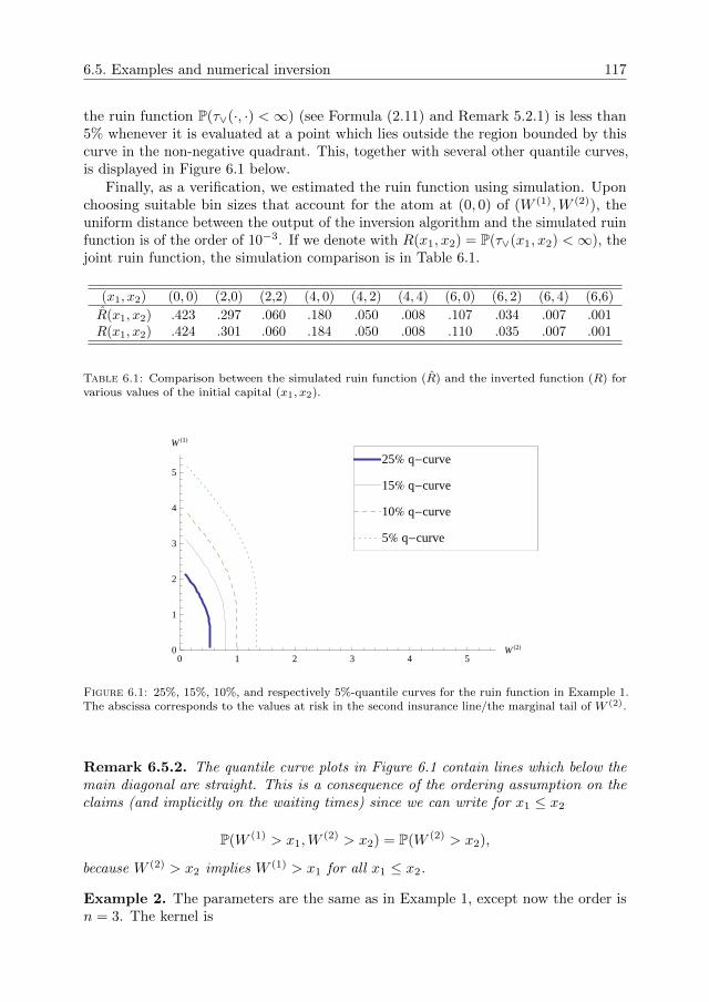
6.5. Examples and numerical inversion 117

the ruin function P(τ∨(·, ·) <∞) (see Formula (2.11) and Remark 5.2.1) is less than5% whenever it is evaluated at a point which lies outside the region bounded by thiscurve in the non-negative quadrant. This, together with several other quantile curves,is displayed in Figure 6.1 below.

Finally, as a verification, we estimated the ruin function using simulation. Uponchoosing suitable bin sizes that account for the atom at (0, 0) of (W (1),W (2)), theuniform distance between the output of the inversion algorithm and the simulated ruinfunction is of the order of 10−3. If we denote with R(x1, x2) = P(τ∨(x1, x2) <∞), thejoint ruin function, the simulation comparison is in Table 6.1.

(x1, x2) (0, 0) (2,0) (2,2) (4, 0) (4, 2) (4, 4) (6, 0) (6, 2) (6, 4) (6,6)

R(x1, x2) .423 .297 .060 .180 .050 .008 .107 .034 .007 .001R(x1, x2) .424 .301 .060 .184 .050 .008 .110 .035 .007 .001

Table 6.1: Comparison between the simulated ruin function (R) and the inverted function (R) forvarious values of the initial capital (x1, x2).

0 1 2 3 4 5W H2L0

1

2

3

4

5

W H1L

5% q-curve

10% q-curve

15% q-curve

25% q-curve

Figure 6.1: 25%, 15%, 10%, and respectively 5%-quantile curves for the ruin function in Example 1.The abscissa corresponds to the values at risk in the second insurance line/the marginal tail of W (2).

Remark 6.5.2. The quantile curve plots in Figure 6.1 contain lines which below themain diagonal are straight. This is a consequence of the ordering assumption on theclaims (and implicitly on the waiting times) since we can write for x1 ≤ x2

P(W (1) > x1,W(2) > x2) = P(W (2) > x2),

because W (2) > x2 implies W (1) > x1 for all x1 ≤ x2.

Example 2. The parameters are the same as in Example 1, except now the order isn = 3. The kernel is

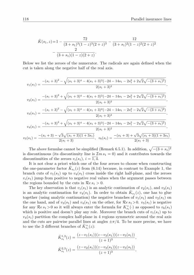
118 Parallel insurance lines

K(s1, z)=1− 72

(3 + s1)3(1− z)3(2 + z)3− 12

(3 + s1)2(1− z)2(2 + z)2

− 2

(3 + s1)(1− z)(2 + z).

Below we list the zeroes of the numerator. The radicals are again defined when thecut is taken along the negative half of the real axis.

v1(s1) =−(s1 + 3)2 −

√(s1 + 3)4 − 4(s1 + 3)2(−24− 14s1 − 2s21 + 2

√2√−(3 + s1)2)

2(s1 + 3)2,

v2(s1) =−(s1 + 3)2 +

√(s1 + 3)4 − 4(s1 + 3)2(−24− 14s1 − 2s21 + 2

√2√−(3 + s1)2)

2(s1 + 3)2,

v3(s1) =−(s1 + 3)2 −

√(s1 + 3)4 − 4(s1 + 3)2(−24− 14s1 − 2s21 − 2

√2√−(3 + s1)2)

2(s1 + 3)2,

v4(s1) =−(s1 + 3)2 +

√(s1 + 3)4 − 4(s1 + 3)2(−24− 14s1 − 2s21 − 2

√2√−(3 + s1)2)

2(s1 + 3)2,

v5(s1) =−(s1 + 3)−

√3√

(s1 + 3)(1 + 3s1)

2(s1 + 3), v6(s1) =

−(s1 + 3) +√

3√

(s1 + 3)(1 + 3s1)

2(s1 + 3).

The above formulae cannot be simplified (Remark 6.5.1). In addition,√−(3 + s1)2

is discontinuous (its discontinuity line is Ims1 = 0) and it contributes towards thediscontinuities of the zeroes vi(s1), i = 1, 4.

It is not clear a priori which one of the four zeroes to choose when constructingthe one-parameter factor Ks1(z) from (6.14) because, in contrast to Example 1, thebranch cuts of v1(s1) up to v4(s1) cross inside the right half-plane, and the zeroesvi(s1) jump from positive to negative real values when the argument passes betweenthe regions bounded by the cuts in Re s1 > 0.

The key observation is that v1(s1) is an analytic continuation of v2(s1), and v3(s1)is an analytic continuation for v4(s1). In order to obtain Ks1(z), one has to gluetogether (using analytic continuation) the negative branches of v1(s1) and v2(s1) onthe one hand, and of v3(s1) and v4(s1) on the other, for Re s1>0. v5(s1) is negativefor any Re s1>0 so it will always enter the formula for K+

s1(·) as opposed to v6(s1)which is positive and doesn’t play any role. Moreover the branch cuts of v1(s1) up tov4(s1) partition the complex half-plane in 4 regions symmetric around the real axisand the cuts are pairwise parallel lines at angles ±π/4. To be more precise, we haveto use the 3 different branches of K+

s1(z):

K1,3s1 (z) =

(z−v1(s1))(z−v3(s1))(z−v5(s1))

(z + 1)3,

K2,3s1 (z) =

(z−v2(s1))(z−v3(s1))(z−v5(s1))

(z + 1)3,

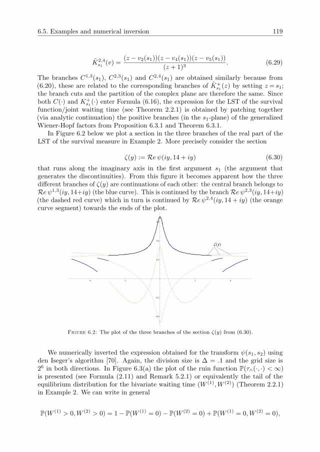
6.5. Examples and numerical inversion 119

K2,4s1 (v) =

(z − v2(s1))(z − v4(s1))(z − v5(s1))

(z + 1)3. (6.29)

The branches C1,3(s1), C2,3(s1) and C2,4(s1) are obtained similarly because from(6.20), these are related to the corresponding branches of K+

s1(z) by setting z= s1;the branch cuts and the partition of the complex plane are therefore the same. Sinceboth C(·) and K+

s1(·) enter Formula (6.16), the expression for the LST of the survivalfunction/joint waiting time (see Theorem 2.2.1) is obtained by patching together(via analytic continuation) the positive branches (in the s1-plane) of the generalizedWiener-Hopf factors from Proposition 6.3.1 and Theorem 6.3.1.

In Figure 6.2 below we plot a section in the three branches of the real part of theLST of the survival measure in Example 2. More precisely consider the section

ζ(y) := Reψ(iy, 14 + iy) (6.30)

that runs along the imaginary axis in the first argument s1 (the argument thatgenerates the discontinuities). From this figure it becomes apparent how the threedifferent branches of ζ(y) are continuations of each other: the central branch belongs toReψ1,3(iy, 14+iy) (the blue curve). This is continued by the branchReψ2,3(iy, 14+iy)(the dashed red curve) which in turn is continued by Reψ2,4(iy, 14 + iy) (the orangecurve segment) towards the ends of the plot.

ΖHyL

-4 -2 2 4

-0.4

-0.2

0.2

0.4

0.6

Figure 6.2: The plot of the three branches of the section ζ(y) from (6.30).

We numerically inverted the expression obtained for the transform ψ(s1, s2) usingden Iseger’s algorithm [70]. Again, the division size is ∆ = .1 and the grid size is26 in both directions. In Figure 6.3(a) the plot of the ruin function P(τ∧(·, ·) < ∞)is presented (see Formula (2.11) and Remark 5.2.1) or equivalently the tail of theequilibrium distribution for the bivariate waiting time (W (1),W (2)) (Theorem 2.2.1)in Example 2. We can write in general

P(W (1) > 0,W (2) > 0) = 1− P(W (1) = 0)− P(W (2) = 0) + P(W (1) = 0,W (2) = 0),

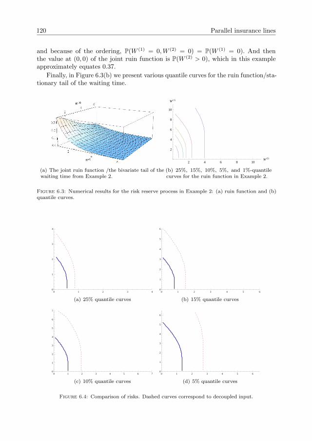
120 Parallel insurance lines

and because of the ordering, P(W (1) = 0,W (2) = 0) = P(W (1) = 0). And thenthe value at (0, 0) of the joint ruin function is P(W (2) > 0), which in this exampleapproximately equates 0.37.

Finally, in Figure 6.3(b) we present various quantile curves for the ruin function/sta-tionary tail of the waiting time.

(a) The joint ruin function /the bivariate tail of thewaiting time from Example 2.

2 4 6 8 10W H2L

2

4

6

8

10

W H1L

(b) 25%, 15%, 10%, 5%, and 1%-quantilecurves for the ruin function in Example 2.

Figure 6.3: Numerical results for the risk reserve process in Example 2: (a) ruin function and (b)quantile curves.

0 1 2 3 40

1

2

3

4

(a) 25% quantile curves

0 1 2 3 4 5 60

1

2

3

4

5

6

(b) 15% quantile curves

0 1 2 3 4 5 6 70

1

2

3

4

5

6

7

(c) 10% quantile curves

0 1 2 3 4 5 60

1

2

3

4

5

6

(d) 5% quantile curves

Figure 6.4: Comparison of risks. Dashed curves correspond to decoupled input.

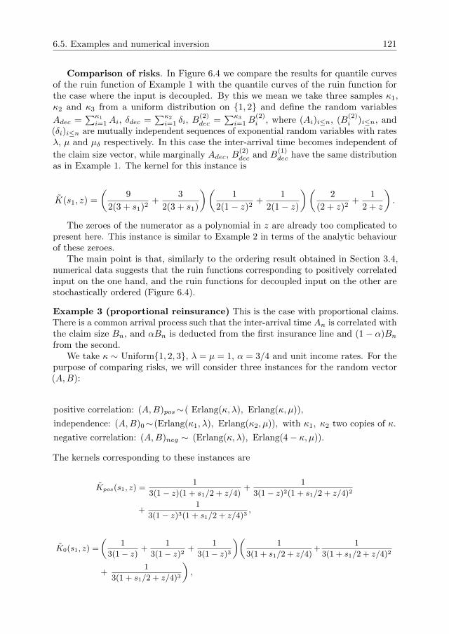
6.5. Examples and numerical inversion 121

Comparison of risks. In Figure 6.4 we compare the results for quantile curvesof the ruin function of Example 1 with the quantile curves of the ruin function forthe case where the input is decoupled. By this we mean we take three samples κ1,κ2 and κ3 from a uniform distribution on {1, 2} and define the random variables

Adec =∑κ1

i=1Ai, δdec =∑κ2

i=1 δi, B(2)dec =

∑κ3

i=1B(2)i , where (Ai)i≤n, (B

(2)i )i≤n, and

(δi)i≤n are mutually independent sequences of exponential random variables with ratesλ, µ and µδ respectively. In this case the inter-arrival time becomes independent of

the claim size vector, while marginally Adec, B(2)dec and B

(1)dec have the same distribution

as in Example 1. The kernel for this instance is

K(s1, z) =

(9

2(3 + s1)2+

3

2(3 + s1)

)(1

2(1− z)2+

1

2(1− z)

)(2

(2 + z)2+

1

2 + z

).

The zeroes of the numerator as a polynomial in z are already too complicated topresent here. This instance is similar to Example 2 in terms of the analytic behaviourof these zeroes.

The main point is that, similarly to the ordering result obtained in Section 3.4,numerical data suggests that the ruin functions corresponding to positively correlatedinput on the one hand, and the ruin functions for decoupled input on the other arestochastically ordered (Figure 6.4).

Example 3 (proportional reinsurance) This is the case with proportional claims.There is a common arrival process such that the inter-arrival time An is correlated withthe claim size Bn, and αBn is deducted from the first insurance line and (1− α)Bnfrom the second.

We take κ ∼ Uniform{1, 2, 3}, λ = µ = 1, α = 3/4 and unit income rates. For thepurpose of comparing risks, we will consider three instances for the random vector(A,B):

positive correlation: (A,B)pos∼( Erlang(κ, λ), Erlang(κ, µ)),

independence: (A,B)0∼(Erlang(κ1, λ), Erlang(κ2, µ)), with κ1, κ2 two copies of κ.

negative correlation: (A,B)neg ∼ (Erlang(κ, λ), Erlang(4− κ, µ)).

The kernels corresponding to these instances are

Kpos(s1, z) =1

3(1− z)(1 + s1/2 + z/4)+

1

3(1− z)2(1 + s1/2 + z/4)2

+1

3(1− z)3(1 + s1/2 + z/4)3,

K0(s1, z) =

(1

3(1− z)+

1

3(1− z)2+

1

3(1− z)3

)(1

3(1 + s1/2 + z/4)+

1

3(1 + s1/2 + z/4)2

+1

3(1 + s1/2 + z/4)3

),

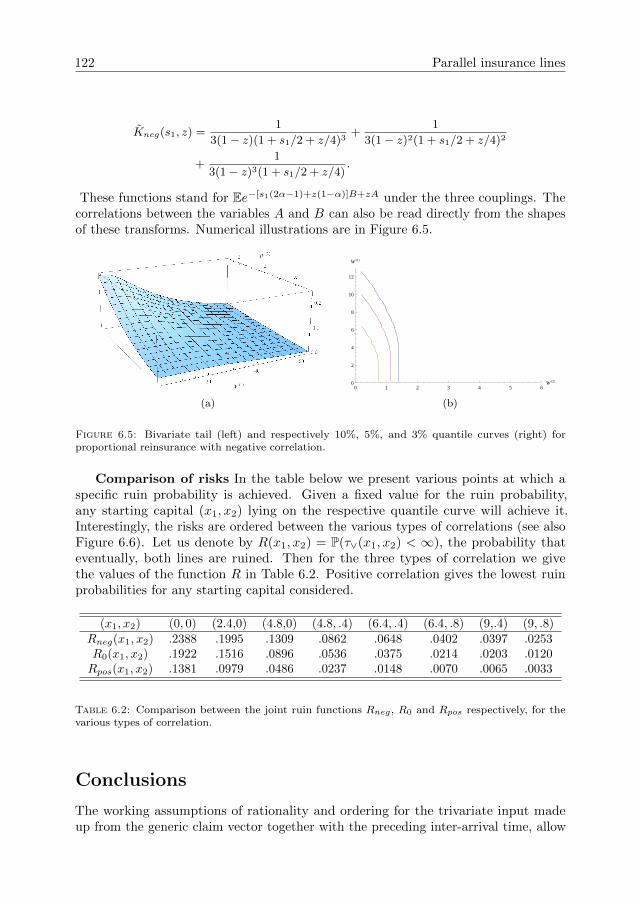
122 Parallel insurance lines

Kneg(s1, z) =1

3(1− z)(1 + s1/2 + z/4)3+

1

3(1− z)2(1 + s1/2 + z/4)2

+1

3(1− z)3(1 + s1/2 + z/4).

These functions stand for Ee−[s1(2α−1)+z(1−α)]B+zA under the three couplings. Thecorrelations between the variables A and B can also be read directly from the shapesof these transforms. Numerical illustrations are in Figure 6.5.

(a)

0 1 2 3 4 5 6W H2L0

2

4

6

8

10

12

W H1L

(b)

Figure 6.5: Bivariate tail (left) and respectively 10%, 5%, and 3% quantile curves (right) forproportional reinsurance with negative correlation.

Comparison of risks In the table below we present various points at which aspecific ruin probability is achieved. Given a fixed value for the ruin probability,any starting capital (x1, x2) lying on the respective quantile curve will achieve it.Interestingly, the risks are ordered between the various types of correlations (see alsoFigure 6.6). Let us denote by R(x1, x2) = P(τ∨(x1, x2) < ∞), the probability thateventually, both lines are ruined. Then for the three types of correlation we givethe values of the function R in Table 6.2. Positive correlation gives the lowest ruinprobabilities for any starting capital considered.

(x1, x2) (0, 0) (2.4,0) (4.8,0) (4.8, .4) (6.4, .4) (6.4, .8) (9,.4) (9, .8)Rneg(x1, x2) .2388 .1995 .1309 .0862 .0648 .0402 .0397 .0253R0(x1, x2) .1922 .1516 .0896 .0536 .0375 .0214 .0203 .0120Rpos(x1, x2) .1381 .0979 .0486 .0237 .0148 .0070 .0065 .0033

Table 6.2: Comparison between the joint ruin functions Rneg, R0 and Rpos respectively, for thevarious types of correlation.

Conclusions

The working assumptions of rationality and ordering for the trivariate input madeup from the generic claim vector together with the preceding inter-arrival time, allow

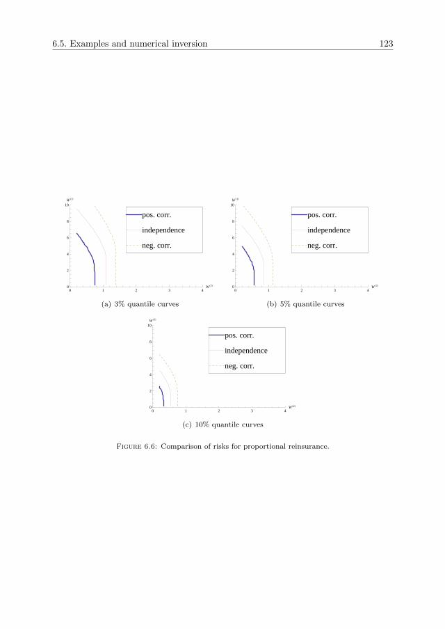
6.5. Examples and numerical inversion 123

0 1 2 3 4W H2L0

2

4

6

8

10W H1L

neg. corr.

independence

pos. corr.

(a) 3% quantile curves

0 1 2 3 4W H2L0

2

4

6

8

10W H1L

neg. corr.

independence

pos. corr.

(b) 5% quantile curves

0 1 2 3 4W H2L0

2

4

6

8

10W H1L

neg. corr.

independence

pos. corr.

(c) 10% quantile curves

Figure 6.6: Comparison of risks for proportional reinsurance.

124 Parallel insurance lines

one to obtain detailed numerical results for the joint ruin probability as a functionof the initial risk reserves. Our numerical results suggest that when comparing ruinfunctions that correspond to various correlation structures between claim intervals andclaim sizes, positive correlation among these cause lower values of the ruin probabilitycompared to zero correlation, and even more so, when compared to negative correlation.

By using the relations described in Section 2.2, one can recover the other types ofruin or survival functions, where the numerical inversion of the marginal transforms,when needed, can be carried out using the one-dimensional inversion algorithm.

6.6 Appendix C

Proposition 6.6.1 (On the zeroes of the kernel 1−K(s1, z)). For each s1, Re s1 ≥ 0,g(s1, z)− f(s1, z) and g(s1, z) have the same number of zeroes in Re z ≥ 0.

Proof. We show that g(s1, z) dominates f(s1, z) on a suitably chosen contour in thecomplex z-plane. From this the claim in the proposition will follow via Rouche’stheorem [102], p. 116. Consider the contour which is made up from the extended arc:

Cε :={reiϕ; ϕ ∈ [−π/2− arccos ε, π/2 + arccos ε]

},

together with the line segment

I :={−ε+ iω; |ω| ∈

[0, r√

1− ε2]}

.

The rationality of the transform ensures that K(s1, z) can be analytically continued ona thin strip: Re z < 0, |Re z| < ε. We first consider the contour Cε. On the one handwe have the triangle inequality for f : |f(s1, z)| ≤ f(|s1|, |z|), where f is a polynomialwith the same degree as f . On the other hand, if we represent gs1(z) for fixed s1 asgs1(z) = am(s1)

∏i(z − ξi(s1)), with ξi(s1) its zeroes and am(s1) the coefficient of zm,

m = m(s1) = deg gs1(z), then the same triangle inequality gives a lower bound for|g(s1, z)|:

|g(s1, z)| = |am(s1)|∏i

|z − ξi(s1)| ≥ |am(s1)|∏i

(|z| − |ξi(s1)|) =: g(s1, |z|),

with the remark that gs1(|z|) has the same degree as gs1(z).

Now we can bound for r sufficiently large, such that the interior of Cε ∪ I containsall the zeroes of gs1(|z|) and z ∈ Cε:∣∣∣∣f(s1, z)

g(s1, z)

∣∣∣∣ ≤ f(|s1|, |z|)g(s1, |z|)

→ 0, as r →∞.

Convergence holds because the degree of the numerator is strictly less than that ofthe denominator, by Assumption 6.1.1. This establishes the bound |g(s1, z)| > |f(s1, z)|on Cε, for r large enough.

6.6. Appendix C 125

For the segment I, we use the safety loading condition for the second(!) line:

c2EA− EB(2) > 0. That is, we start with the fact ddz

f(0,z)g(0,z) |z=0 = c2EA− EB(2) > 0.

So for ε > 0 sufficiently small, f(0,−ε)g(0,−ε) <

f(0,0)g(0,0) = 1. Then we can write for z ∈ I:

∣∣∣∣f(s1, ε+ iω)

g(s1, ε+ iω)

∣∣∣∣ ≤ E(|e−s1δ| · |e−ε(A−B(2))| · |e−iω(A−B(2))|)

≤ Ee−ε(A−B(2)) =f(0,−ε)g(0,−ε) < 1.

Above we used the rough bound |e−s1δ| ≤ 1. This completes the proof.Notice that the key role in the proof is played by ρ2 < 1 and not ρ1 < 1 (ρ2 < ρ1).

Chapter 7

Proportional reinsurance withsubexponential claims

In this chapter, we will study the asymptotic behaviour of the ruin probability fora large initial capital for a proportional reinsurance contract. This problem can beformulated as the first crossing probability of the process of aggregate claims abovea non-linear barrier. A detailed description of the problem is given in Section 7.1;the main result and its probabilistic interpretation is given in Section 7.2. The ’onelarge jump that causes ruin’ heuristic is shown to be asymptotically valid as the initialcapital grows arbitrarily large along a ray in the plane. The proofs and the technicalresults are found in Section 7.3.

This is part of an ongoing project with Sergey Foss, Zbigniew Palmowski andTomasz Rolski, and the contents of this chapter are slightly related to an unpublishedmanuscript of S. Foss, T. Rolski and S. Zachary [62].

7.1 Introduction

Palmowski and Pistorius [91] studied boundary crossing probabilities of a stochasticprocess with regularly varying increments. This study was motivated by ruin proba-bilities of two insurance companies with proportional claims (see Avram et al. [20])and the steady state distribution of a tandem queue with two servers (see Lieshoutand Mandjes [86]). In this paper we generalize this result to the case of a stronglysubexponential distribution of increments. We define

St =

n(t)∑k=1

Bk (7.1)

for n(t) a renewal process with i.i.d. inter-arrival times Ak, and the claims Bk arei.i.d. random variables independent of n(t), with the distribution function F (x). Letthe barriers b1, b2 be given by

b1(t) = b1(t;x1) = x1 + p1t, b2(t) = b2(t;x2) = x2 + p2t,

127

128 Proportional reinsurance

where xi = u(i)/δi, pi = ci/δi, with δi being the specific proportion used to split aclaim B, δ1 + δ2 = 1, so that risk reserve i receives claim sizes distributed as δiB,i = 1, 2. We assume that

p1 > p2, p2 > EB/EA, (7.2)

for generic A and B. We will consider the following boundary crossing probabilities:

ψ∧(x1, x2) = P(∃t ≥ 0 : St > (x1 + p1t) ∧ (x2 + p2t)),

ψ∨(x1, x2) = P(∃t ≥ 0 : St > (x1 + p1t) ∨ (x2 + p2t)),

where x ∨ y = max{x, y} and x ∧ y = min{x, y}.The ψ∧(x1, x2) describes the ruin probability of at least one insurance company,

and ψ∨(x1, x2) corresponds to the eventual ruin of both insurance companies. Thefirst assumption in (7.2) means that the second company receives less premium peramount paid out and the second one is the stability condition under which the surpluslevels of both insurance companies tend to infinity. The solutions of the ”degeneratetwo-dimensional” ruin problems strongly depend on the position of the vector ofpremium rates p = (p1, p2). Namely, if the initial capital levels satisfy x2 ≤ x1, thetwo lines do not intersect, hence the ”∧−” and the ”∨−”ruin always happen forthe second and first company respectively. In this case the asymptotics follow fromone-dimensional ruin theory – see e.g. Rolski et al. [96]. Therefore we focus here onthe opposite case, when x1 < x2.

In this chapter, we derive the exact first order asymptotics of these ruin probabilitiesif x1, x2 tend to infinity along a ray in the positive quadrant (i.e. x1/x2 = a < 1 isconstant) if the claims follow a subexponential distribution. We model the claims bysubexponential distributions since many catastrophic events like earthquakes, storms,terrorist attacks etc. are modelled by them. Insurance companies use e.g. theLognormal distribution (which is subexponential) to model car claims – see Foss et al.[60], Rolski et al. [96] or Embrechts et al. [53] for further background.

The chapter is organized as follows. In the next section we present the main resultswhich will be proved in Section 7.3.

7.2 Main results

In order to state our results we start with recalling some notions. We assume thatinter-arrival times (Ak)k are light-tailed, that is E exp{θA} <∞ for some θ > 0 andgeneric A. Moreover, we assume that the distribution F of a generic claim B ≥ 0belongs to the class S of subexponential distribution functions, where a distributionfunction G ∈ S if and only if G(x) > 0 for all x and

limx→∞

G∗2(x)/G(x) = 2 (7.3)

(where G∗2 is the convolution of G with itself). Here G denotes the tail distributiongiven by G(x) = 1 − G(x). The above means that asymptotically, the only way in

7.3. Proof of the main result 129

which a sum of two independent copies from G can be large is that precisely one ofthem is large. Since these are independent copies, any one of them is equally likely tobe the large one, hence the limit above, having a combinatorial flavor. This limit canbe extended by induction to the n-fold convolution, and then the limit becomes n, seeFoss et al. [60], Cor. 3.20.

We further assume throughout that F ∈ S∗, the class of strong subexponentialdistributions. A distribution function G on R belongs to the class S∗ if G(x) > 0 forall x, and ∫ x

0

G(x− y)G(y) dy ∼ 2mGG(x), as x→∞, (7.4)

where we denote f(x) ∼ g(x) to mean limx→∞ f(x)/g(x) = 1. The constant mG

represents

mG =

∫ ∞0

G(x) dx.

It is known that the property G ∈ S∗ depends only on the tail of G. Further, if G ∈ S∗then G ∈ S and also Gs ∈ S∗, where

Gs(x) = min

(1,

∫ ∞x

G(t) dt

)is the integrated, or second-tail, distribution function determined by G; see Foss et al.[60] §3.4 for details.

Theorem 7.2.1. We have, for a < 1:

ψ∧(aK,K) ∼ H(K), (7.5)

ψ∨(aK,K) ∼ U(K), (7.6)

as K →∞, where

H(K) =

∞∫0

F (min{aK + t(p1EA− EB),K + t(p2EA− EB)})dt,

U(K) =

∞∫0

F (max{aK + t(p1EA− EB),K + t(p2EA− EB)})dt.

7.3 Proof of the main result

Before we give the formal proof, we owe some explanations. Identities (7.5) and (7.6)can be explained by the ’single large jump’ principle, that is, for large values of thestarting capital, the most likely way in which the corresponding type of ruin canhappen is through a single large claim that makes the aggregate claims process Snjump directly above the corresponding barrier. Up to the time of ruin, the risk reserveprocess behaves in a typical way - looked at on a large scale, component i drifts

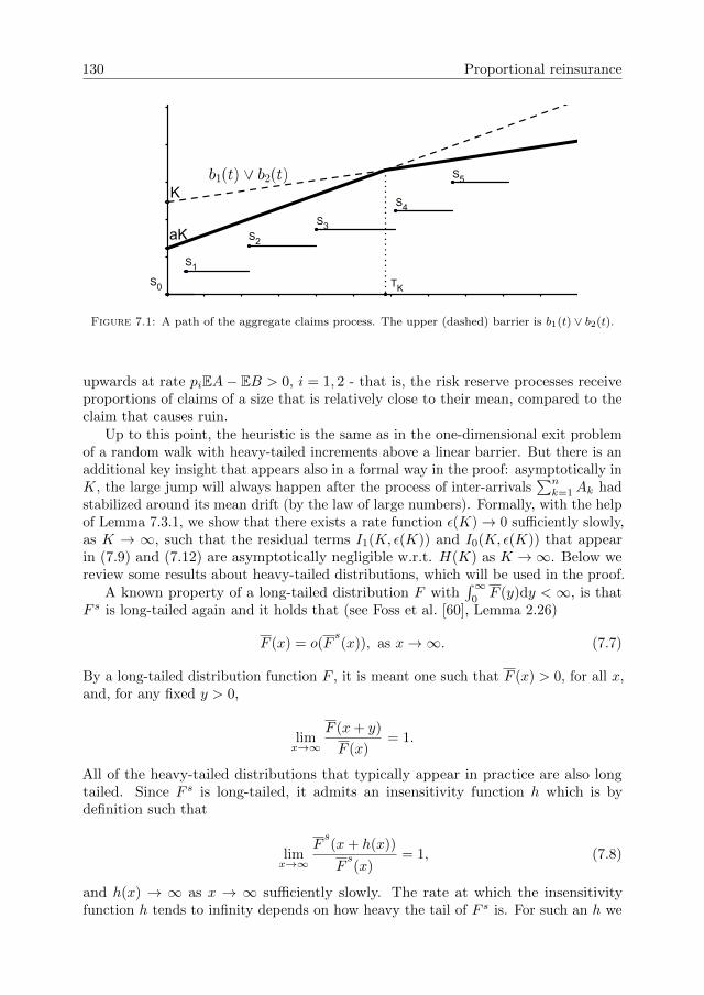
130 Proportional reinsurance

Figure 7.1: A path of the aggregate claims process. The upper (dashed) barrier is b1(t) ∨ b2(t).

upwards at rate piEA− EB > 0, i = 1, 2 - that is, the risk reserve processes receiveproportions of claims of a size that is relatively close to their mean, compared to theclaim that causes ruin.

Up to this point, the heuristic is the same as in the one-dimensional exit problemof a random walk with heavy-tailed increments above a linear barrier. But there is anadditional key insight that appears also in a formal way in the proof: asymptotically inK, the large jump will always happen after the process of inter-arrivals

∑nk=1Ak had

stabilized around its mean drift (by the law of large numbers). Formally, with the helpof Lemma 7.3.1, we show that there exists a rate function ε(K)→ 0 sufficiently slowly,as K → ∞, such that the residual terms I1(K, ε(K)) and I0(K, ε(K)) that appearin (7.9) and (7.12) are asymptotically negligible w.r.t. H(K) as K →∞. Below wereview some results about heavy-tailed distributions, which will be used in the proof.

A known property of a long-tailed distribution F with∫∞

0F (y)dy < ∞, is that

F s is long-tailed again and it holds that (see Foss et al. [60], Lemma 2.26)

F (x) = o(Fs(x)), as x→∞. (7.7)

By a long-tailed distribution function F , it is meant one such that F (x) > 0, for all x,and, for any fixed y > 0,

limx→∞

F (x+ y)

F (x)= 1.

All of the heavy-tailed distributions that typically appear in practice are also longtailed. Since F s is long-tailed, it admits an insensitivity function h which is bydefinition such that

limx→∞

Fs(x+ h(x))

Fs(x)

= 1, (7.8)

and h(x) → ∞ as x → ∞ sufficiently slowly. The rate at which the insensitivityfunction h tends to infinity depends on how heavy the tail of F s is. For such an h we

7.3. Proof of the main result 131

can strengthen the asymptotic behaviour (7.7) to

h(x)F (x) = o(Fs(x)),

and this will be a useful consequence for our purposes, see (7.14) and (7.16).

Proof of Theorem 7.2.1. Let Sn =∑nk=1Bk and Sn := Sn − nEB be the centered

random walk. Denote by

N∗ε = inf{n : ∀k ≥ n, tk ∈ [(EA− ε)k, (EA+ ε)k]}

for some ε > 0, to be the first time the random walk tn =∑nk=1Ak will stabilize

around its mean. By the strong law of large numbers (SLLN), we have N∗ε <∞ a.s.and we can bound

I2 ≤ ψ∧(aK,K) ≤ I1 + I2, (7.9)

where

I1 := P(∃n ≤ N∗ε : Sn > min{aK + p1tn − nEB,K + p2tn − nEB})I2 := P(∃n > N∗ε : Sn > min{aK + p1tn − nEB,K + p2tn − nEB})

We will show below that I1 = o(H(K)) and I2 ∼ H(K), as K →∞. Observe that, bythe definition of N∗ε ,

I2 ≤ P(∃n ≥ 0 : Sn > min{aK+p1(EA−ε)n−nEB,K+p2(EA−ε)n−nEB}). (7.10)

If we denote with g(n) := min{aK+p1(EA− ε)n−nEB,K+p2(EA− ε)n−nEB}that appears inside the upper bound in (7.10), then we will have for some positive c

g(n+ 1) ≥ g(n) + c,

and if we take ε > 0 sufficiently small, we can choose 0 < c < p2EA− EB − p2ε, andsuch that it does not depend on ε. From the main result of Foss et al. [61], the upperbound in (7.10) is asymptotically equivalent to:

(1+ δc(K))

∞∫0

F (min{aK+(p1EA−EB−p1ε)t,K+(p2EA−EB−p2ε)t})dt, (7.11)

with δc(K)→ 0 as K →∞. This establishes the asymptotic behaviour of the upperbound of I2. Now we turn to the lower bound on I2.

I2 ≥ P(∃n ≥ 0 : Sn > min{aK + p1(EA+ ε)n− nEB,K + p2(EA+ ε)n− nEB})− P(∃n ≤ N∗ε : Sn > min{aK + p1(EA+ ε)n− nEB,K + p2(EA+ ε)n− nEB}).

(7.12)

We denote the second increment on the RHS of the above inequality by I0. We willshow below that this together with I1 is asymptotically negligible o(H(K)) as K →∞.

132 Proportional reinsurance

Using again the main result in Foss et al. [61], gives the asymptotic behaviour of thefirst term on the RHS of (7.12):

(1−δc(aK))

∞∫0

F (min{aK+(p1EA−EB+p1ε)t,K+(p2EA−EB+p2ε)t})dt. (7.13)

We will prove now that for sufficiently small ε > 0,

I1 = P(∃n ≤ N∗ε : Sn > min{aK + p1tn − nEB,K + p2tn − nEB})

and

I0 = P(∃n ≤ N∗ε : Sn > min{aK + p1(EA+ ε)n− nEB,K + p2(EA+ ε)n− nEB})

are asymptotically negligible.Since F s ∈ S∗, a useful characterization of long-tailed distribution functions yields

the existence of a non decreasing function h : R+ → R+ such that h(x) → ∞ asx→∞ and (7.8) holds. An immediate consequence of this insensitivity property isthat (see Foss et al. [60], Lemmae 2.19, 2.25),

h(x)F (x) = o(F s(x)). (7.14)

Since N∗ε is independent of Sn, we have the following upper bound for both I0 andI1 (see [60], Thm. 3.37, Cor. 3.20):

I0, I1 ≤ P(∃n ≤ N∗ε : Sn > aK) ∼ EN∗ε F (aK), (7.15)

once we show that EN∗ε < ∞ for any ε > 0. The latter statement follows fromCramer’s Large Deviations Principle (LDP) for the light-tailed sequence {Ak}k≥1,which has the good rate function Λ∗(x):

P(|tl| ≥ εl) ≤ 2e−l infx≥ε Λ∗(x),

with tl :=∑li=1Ai − lEA, so that we can write

P(N∗ε > k) ≤∑l≥kP(|tl| ≥ εl) ≤

∑l≥k

2e−I(ε)l ≤ Cεe−I(ε)k,

with I(ε) := infx≥ε Λ∗(x), and Cε is some positive constant that depends on ε. SeeCramer’s Theorem 2.2.3 and the subsequent Remark c) in Dembo and Zeitouni [49],p. 27. For the arguments below, it is essential that EN∗ε explodes as ε tends to 0.

Define f(x) := EN∗1/x; by construction, f is non-decreasing and f(x) → ∞ as

x → ∞. We show in Lemma 7.3.1 that there exists a non-negative function f∗(y),such that f∗(y)→∞ as y →∞ and

f ◦ f∗(y) ≤ y, for all y > 0.

With this construction, take ε = 1/f∗(h(K)), so that we have by the definitions of f∗

and of h that

7.3. Proof of the main result 133

EN∗ε = f ◦ f∗ ◦ h(K) ≤ h(K),

and from (7.15), with this choice for ε, the asymptotic behaviour of the upper boundon I1(K) and I0(K) is

EN∗ε F (aK) ≤ h(K)F (aK) = o(F s(aK)) = o(H(K)), (7.16)

by virtue of (7.14). This completes the argument for the asymptotic behaviour ofI1(K) and I0(K).

All that is left is a limit argument for taking ε→ 0. Let us denote the integratedtails that appear in (7.11) and (7.13)

H−ε(K) :=

∞∫0

F (min{aK + (p1EA− EB − p1ε)t,K + (p2EA− EB − p2ε)t})dt,

Hε(K) :=

∞∫0

F (min{aK + (p1EA− EB + p1ε)t,K + (p2EA− EB + p2ε)t})dt.

(7.17)

It follows from Lemma 7.3.2 below that both Hε(K)/H(K) and H−ε(K)/H(K)converge to 1 as K →∞. The proof of (7.5) is complete because we can now write forε small, using (7.10), (7.11), (7.13) and (7.16):

(1− δc(aK))Hε(K)

H(K)− o(1) ≤ ψ∧(K)

H(K)≤ (1 + δc(aK))

H−ε(K)

H(K)+ o(1), K →∞,

and with the choice ε(K) = 1/f∗(h(K)).The proof of (7.6) follows along exactly the same lines. The only place where the

shape of the barrier is used is Lemma 7.3.2. But also in this case, it can be shown thatthe corresponding functionals U−ε, Uε are proportional to U , and the proportionalityconstants tend to 1 as ε→ 0. This completes the proof.

Lemma 7.3.1. Let f : R+ → R+ be a non-decreasing function such that f(x)→∞as x → ∞. Then there exists a non-decreasing function f∗ : R+ → R+ such thatf∗(y)→∞ as y →∞ and

f ◦ f∗(y) ≤ y, for all y > 0.

Proof of Lemma 7.3.1. There are several possible choices for f∗. A natural one isthe following: let f+ be the right-continuous version of f . Since f is non-decreasing,f(x) ≤ f+(x). For a fixed y, set

f∗(y) := sup{x; f+(x) ≤ y}.

We have by construction that

134 Proportional reinsurance

f+ ◦ f∗(y) ≤ y.Since f is non-decreasing, we can write

f ◦ f∗(y) ≤ f+ ◦ f∗(y) ≤ y. (7.18)

The monotonicity of f∗ together with f∗(y)→∞ as y →∞ follow from its definitionand the assumption f(x) → ∞. Thus f∗ is constructed as the right-inverse of f+,and this is the mirror-image construction of the well known quantile function (the leftinverse) of a non-decreasing and right-continuous function – a c.d.f. (see Embrechtsand Hofert [52] for the analogue of (7.18)). The proof is complete.

Lemma 7.3.2. With the notations and definitions from the proof of Theorem 7.2.1,the functions Hε(K), H(K) and H−ε(K) are proportional for any K > 0 and ε > 0:

Hε(K) =m1

mε,1H(K).

H−ε(K) =m1

m−ε,1H(K).

Here we denoted by mi := piEA− EB and m±ε,i := pi(EA± ε)− EB.

Proof of Lemma 7.3.2.

Define T := (1−a)Km1−m2

the (unique) crossing epoch of lines aK +m1t and K +m2tand let

T±ε :=(1− a)K

(m±ε,1 −m±ε,2)

be the (unique) epochs at which the lines aK + p1(EA± ε)t− tEB and K + p2(EA±ε)t− tEB cross.

There are several key relations that these crossing times satisfy, and they are easyto check:

mε,1Tε = m1T, mε,2Tε = m2T,m1

mε,1=

m2

mε,2. (7.19)

Similar relations hold for T−ε and m−ε,i. Using the above definitions, we can write

H(K) =1

m1

aK+m1T∫aK

F (u)du+1

m2

∞∫K+m2T

F (u)du,

Hε(K) =1

mε,1

aK+mε,1Tε∫aK

F (u)du+1

mε,2

∞∫K+mε,2Tε

F (u)du,

H−ε(K) =1

m−ε,1

aK+m−ε,1T−ε∫aK

F (u)du+1

m−ε,2

∞∫K+m−ε,2T−ε

F (u)du.

7.3. Proof of the main result 135

Above we partitioned the integrated tails based on the crossing times of the barriersand we changed the variables of integration in each term. We did this in order to bebetter able to compare the three integrated tails.

From (7.19), the integration ends are termwise identical for H(K) and Hε(K).Moreover, using the last identity in (7.19), H(K) and Hε(K) are proportional:

Hε(K) =m1

mε,1H(K).

It follows in the same way as for Hε that

H−ε(K) =m1

m−ε,1H(K).

The proof is complete.

Chapter 8

A coupled processor modelwith simultaneous arrivals

In this chapter we study a coupled processor model which receives service requirementsat both queues simultaneously. We assume that the service requirement at, say, station1 is always greater than the service requirement from station 2. Moreover, when server2 is idle, it switches to process work from the first queue, if there is any. As describedin Section 1.2, for the models introduced by Fayolle and Iasnogorodski [55] and Cohenand Boxma [41], the server i rate is ri when processing from buffer i and r∗j whenprocessing from buffer j, i = 1, 2, j 6= i, so that during an idle period of server i, theother server works at speed rj + r∗j (the notation we use is different than the one usedin [41], but equivalent). By studying the dynamics of this system during infinitesimaltime intervals, it is possible to derive a functional equation for the transform of thejoint amount of work. This analysis was carried out in Cohen [43]. The steady-stateversion of the functional equation for the workload vector (V (1), V (2)) from [43, p. 186,(1.10)] reads, using our notation:

K(s1, s2)ψ(s1, s2) = (r2s2−r∗1s1)ψ1(s1)+(r1s1−r∗2s2)ψ2(s2)+(r∗1s1+r∗2s2)ψ0, (8.1)

with ψ(s1, s2) the Laplace-Stieltjes transform (LST) of the stationary amount of workin the system and with the unknown boundary functions

ψi(si) = E[e−siV(i)

(V (j) = 0)], i 6= j ∈ {1, 2}, ψ0 = P(V (1) = V (2) = 0).

The function K(s1, s2) is the so-called Poisson kernel. For φ(s1, s2) the joint transformof a generic service time vector,

K(s1, s2) = r1s1 + r2s2 − λ[1− φ(s1, s2)].

Actually, in Cohen [43] the functional equation of the time dependent workload isgiven. The stationary version above is obtained by multiplying the functional equation

137

138 A coupled processor model

[43, p. 186, (1.10)] with the discount factor of the Laplace-Stieltjes transform overtime, and then taking the discount factor to 0, while keeping it positive (this is byvirtue of Abel’s theorem).

The analysis in the above mentioned works relies heavily on the theory of complexfunctions which makes it highly non-trivial, and in addition, it is difficult to recognizethe probabilistic nature of the initial problem.

We will show in Section 8.2 that under the additional ordering assumption betweenthe claims, it is possible to relate the coupled processor model to a parallel queueingsystem without coupling. Then the transform of the amount of work in the coupledsystem follows from that obtained in the decoupled parallel system, by using Formula(5.6). This gives an explicit representation for the steady-state amount of work in thecoupled system (Section 8.3), which can be extended to multiple coupled queues bymaking suitable assumptions on the coupling rates (Section 8.4).

8.1 Model description

We consider two parallel M/G/1 queues, with simultaneous arrivals and correlatedservice requirements. The arrival process is a Poisson process with rate λ. Wewill denote by An the time elapsed between arrival epochs n and n + 1, n ≥ 1.The service requirements at the two queues of successive customers are independent,

identically distributed random vectors (B(1)n , B

(2)n ), n ≥ 1. In the sequel we denote with

(B(1), B(2)) a random vector with the same distribution as the vectors (B(1)n , B

(2)n ), n ≥

1. The joint Laplace-Stieltjes transform of this vector is

φ(s1, s2) := E(e−s1B(1)−s2B(2)

).

We will work with the processing rates of server i, when working in buffer j 6= ifor a three dimensional system in Section 8.4. For this reason, let us change the ratesnotation and set c1 and c2 for the servers’ processing rates from their respective bufferand cji , i 6= j for the processing rate of server i in buffer j. An essential assumption inthe model is that, after normalizing the system with the server rates, with probabilityone, each customer has a bigger service requirement in queue 1 than in queue 2, i.e.,

P(B(1)/c1 ≥ B(2)/c2) = 1.

The processors are coupled in the sense that as soon as server 2 becomes idle, itswitches its capacity to serving work from buffer 1 so that it works at rate c12 whenprocessing from buffer 1. Because of the ordering assumption, server 1 will neverbecome idle while server 2 is busy, so there is no need for server 2 to help server 1.We are interested in the joint stationary distribution of the amount of work in the twoqueues. Let us still denote with V (1) the stationary amount of work in queue 1 andwith V (2) the stationary amount of work in queue 2.

Our aim is to study such an interacting queueing system under the above assumptionof ordered service times. In particular we want to find an expression for the Laplace-Stieltjes transform of the joint stationary amount of work.

8.2. Recursive equations for the amount of work in the coupled system 139

8.2 Recursive equations for the amount of work inthe coupled system

In this section we will derive stochastic recursive equations for the joint amount ofwork in the system.

With V(i)tn the amount of work in queue i as seen by customer n upon arrival, we

assume that at time 0 the first customer arrives in an empty system. Then we have

the following recursion for the random variables (V(1)tn , V

(2)tn ), n ≥ 1, which is a special

case of Lindley’s recursion for the coupled processor model (2.14):

(V(1)t1 ,V

(2)t1 ) = (0, 0),

V(1)tn+1

=

[(V

(1)tn +B(1)

n − c1An) ∨ 0 +c12c2

(V(2)tn +B(2)

n − c2An) ∧ 0

]∨ 0, (8.2)

V(2)tn+1

= (V(2)tn +B(2)

n − c2An) ∨ 0.

The second queue evolves without the assistance of the first queue because of theordering assumption. Remark that

− 1

c2[(V

(2)tn +B(2)

n − c2An) ∧ 0]

is the amount of time that server 2 has been idle between the arrival epochs tn and

tn+1 (cf. (1.3)). Then the second term in the recursion of V(1)tn+1

is minus the amount

of work server 2 processes at rate c12 from buffer 1 during his idle period (if it has anidle period).

This extra term appears because the servers are coupled. It is useful to comparethis with the recursion for a system without coupling between the servers. Considertwo parallel queues simultaneously receiving service requirements distributed as thevector (B(1), B(2)). The servers are not coupled anymore and server 1 always works at

speed c1, while server 2 always works at speed c2. Let (V(1)tn , V

(2)tn ) be the amount of

work at arrival epochs in such a system, then the following recursion holds

(V(1)t1 , V

(2)t1 ) = (0, 0),

V(1)tn+1

= (V(1)tn + B(1)

n − c1An) ∨ 0, (8.3)

V(2)tn+1

= (V(2)tn + B(2)

n − c2An) ∨ 0,

with An the inter-arrival time between customer n and n + 1. This is Lindley’srecursion because both queues evolve in isolation as one-dimensional systems. Noticethat, marginally, queue 2 evolves as if there was no coupling in (8.2).

We are ready to give the main result of this section which connects the amountof work in the coupled system to a workload process in a system without couplingbetween the servers. For further usage we will denote by system (C) the coupledsystem and by system (D), the system without coupling.

140 A coupled processor model

Proposition 8.2.1. Let (V(1)tn , V

(2)tn )n≥1 be the workload process at arrival epochs in

system (C). Then the process (V(1)tn +

c12c2V

(2)tn , V

(2)tn )n≥1 is the workload process in a

system of type (D) with generic input of the form (B(1) +c12c2B(2), B(2)), where the

servers have speed (c1 + c12, c2) and do not interact with each other.

We will show that (V(1)tn +

c12c2V

(2)tn , V

(2)tn ) has the same distribution as (V

(1)tn , V

(2)tn ),

the solution to the recursive system (8.3), by using a probabilistic coupling betweensystems (C) and (D), that is we will let the two systems evolve on the same probability

space given by the sequences (An)n≥1 and (B(1)n , B

(2)n )n≥1. The choice for the input

variables in system (D) is the following:

An := An, (B(1)n , B(2)

n ) := (B(1)n +

c12c2B(2)n , B(2)

n ),

c1 := c1 + c12, c2 := c2. (8.4)

To be more precise, start both systems empty at time t1 = 0. At the nth arrival

epoch tn, system (C) receives input (B(1)n , B

(2)n ) whereas system (D) receives input

(B(1)n +

c12c2B

(2)n , B

(2)n ). Let us focus on system (D). The key idea is to partition the

amount of work at queue 1 in system (D) into V(1)t and

c12c2V

(2)t , then during the busy

periods of server 2, distribute the total capacity per time unit c1 + c12 of server 1 in

the following way: c1 is dedicated to processing V(1)t while c12 is used to process the

remainingc12c2V

(2)t . In this way, during the busy periods of server 2, the amount of

work in queue one of system (C) and the work in the c1-dedicated component of queueone in system (D) evolve in the same way.

As soon as queue 2 becomes empty (which now happens at the same moment insystem (C) as in system (D) because the second queue evolves unchanged between the

two systems), in both systems (C) and (D), server 1 will process work V(1)t at speed

c1 + c12. Another remark is that due to the ordering between the service requirements,queue 2 will always become idle before queue 1 in any of the systems (C) or (D) (seealso Remark 8.2.1 below).

We give below the formal proof of Proposition 8.2.1. The idea of the proof is to

verify that V(1)tn +

c12c2V

(2)tn satisfies (8.3) with the input variables from (8.4).

Proof of Proposition 8.2.1. First remark that we can drop the maximum w.r.t. 0 inthe first term of recursion (8.2):

V(1)tn+1

=

[V

(1)tn +B(1)

n − c1An +c12c2

(V(2)tn +B(2)

n − c2An) ∧ 0

]∨ 0, (8.5)

the reason being that the other term is either 0 or negative as pointed out below (8.2),so it can only decrease the term between the square brackets in the recursion of thecoupled queue 1.

Adding the termc12c2V

(2)tn+1

=c12c2

(V(2)tn +B

(2)n − c2An) ∨ 0 to both sides of (8.5) gives

8.3. The transform of the equilibrium amount of work at arrival epochs 141

V(1)tn+1

+c12c2V

(2)tn+1

=

[V

(1)tn +B(1)

n − c1An +c12c2

(V(2)tn +B(2)

n − c2An)

]∨ c

12

c2(V

(2)tn +B(2)

n − c2An) ∨ 0.

We used the fact that the operator ∨ is distributive w.r.t. addition and the obviousdecomposition (x ∧ 0) + (x ∨ 0) = x.

There are two possible cases:

In the event that V(1)tn +B

(1)n − c1An > 0, the RHS above is of the form a ∨ b ∨ 0,

with a > b, hence b can be removed. In the end we can rewrite the above as

V(1)tn+1

+c12c2V

(2)tn+1

=

(V

(1)tn +

c12c2V

(2)tn +B(1)

n +c12c2B(2)n − (c1 + c12)An

)∨ 0.

This is the desired Lindley recursion for V(1)tn +

c12c2V

(2)tn .

In the event that V(1)tn + B

(1)n − c1An < 0, queue 1 would empty at epoch tn+1

without any additional help, so that V(1)tn+1

= 0. Then by the ordering assumption,

V(2)tn+1

= 0 as well, and the above identity is trivially satisfied. The proof is complete andit shows that the ordering between the normalized claims is an essential assumption.

Remark 8.2.1. Notice that the normalized input in the related system (D) remainsordered:

B(1)n +

c12c2B

(2)n

c1 + c12=c1B(1)n

c1+ c12

B(2)n

c2

c1 + c12≥ B

(2)n

c2,

because by assumption, B(1)n /c1 ≥ B(2)

n /c2.

8.3 The transform of the equilibrium amount ofwork at arrival epochs

In Chapter 5 has been shown how to calculate the Laplace-Stieltjes transform of thejoint, stationary amount of work in a system of type (D) under the same orderingassumption (Chapter 5, Formula (5.6)). Thus, by inverting the correspondence fromProposition 8.2.1, and using Remark 8.2.1, we can recover without any additionaleffort the joint transform of (V (1), V (2)), the steady-state amounts of work in thecoupled system. Moreover, because of Poisson arrivals, we have the PASTA property,which means that in equilibrium, the amount of work is the same as the workload seenby an arriving customer.

The inverse relation from Proposition 8.2.1 is

142 A coupled processor model

(V (1), V (2)) = (V (1) − c12c2V (2), V (2)). (8.6)

If we denote by

ψ(C)(s1, s2) := E(e−s1V(1)−s2V (2)

), ψ(D)(s1, s2) := E(e−s1V(1)−s2V (2)

),

the LST of the equilibrium amount of work in system (C) and respectively system(D), then via (8.6), the relation between the LSTs becomes:

ψ(C)(s1, s2) = ψ(D)(s1, s2 − s1c12/c2). (8.7)

Remark 8.3.1. Equation (8.1) can be adapted to describe the stationary workload(V (1), V (2)) in the decoupled system by setting the coupling rates r∗ equal to 0. Thekernel K(s1, s2) has to be modified as well to

K(D)(s1, s2) = (c1 + c12)s1 + c2s2 − λ[1− φ(s1, s2 + s1c12/c2)]

because server 1 receives the extra input c12/c2B(2) and always works at speed c1 + c12.

Then (8.1) becomes

K(D)(s1, s2)ψ(D)(s1, s2) = c2s2ψ(D),1(s1) + (c1 + c12)s1ψ(D),0, (8.8)

since by the ordering relation from Remark 8.2.1, ψ(D),2(s2) is constant and equal toψ(D),0:

ψ(D),2(s2) = E[e−s2V(2)

(V (1) = 0)] = P(V (1) = V (2) = 0) =: ψ(D),0.

On the other hand, the kernel for the coupled system (C) is

K(C)(s1, s2) = c1s1 + c2s2 − λ[1− φ(s1, s2)].

The equation that has to be satisfied by ψ(C)(s1, s2) now reads (with ψ(C),2(s2) ≡ ψ(C),0,again because of the ordering)

K(C)(s1, s2)ψ(C)(s1, s2) = (c2s2 − c12s1)ψ(C),1(s1) + (c1 + c12)s1ψ(C),0 (8.9)

with the key remark that the two boundary functions ψ(D),1(s1) and ψ(C),1(s1) areidentical (Proposition 8.2.1):

E[e−s1V(1)

(V (2) = 0)] ≡ E[e−s1V(1)

(V (2) = 0)]

and the same holds for ψ(C),0 and ψ(D),0.

Now it is easy to check that if ψ(D)(s1, s2) is the solution of (8.8), then ψ(D)(s1, s2−s1c

12/c2) as in (8.7) is the solution of (8.9), and conversely, if ψ(C)(s1, s2) is the solution

8.3. The transform of the equilibrium amount of work at arrival epochs 143

of (8.9) then ψ(C)(s1, s2 + c12/c2s1) is the solution of (8.8). In particular, it followsfrom Chapter 5 that the amount of work in system (C) is ergodic under the condition

lims1→0

s1>0

∂

∂s1K(D)(s1, 0) > 0⇔ E(B(1)) + c12/c2E(B(2)) < (c1 + c12)E(A). (8.10)

This simply means that the first queue in system (D) is capable to handle the amountof input per time unit while working at speed (c1 + c12) and this is sufficient to ensurethat the entire system is stable, because of the ordering assumption. It may happenthat E(B(1)) > c1E(A), i.e. that queue 1 of system (C) would be supercritical if itwere to work only on its own. Inequality (8.10) together with Remark 8.2.1, impliesE(B(2)) < c2E(A), thus queue 2 is ergodic and during its (non-degenerate) idle periodsit is capable to maintain queue 1 stable because of the coupling.

Using the relation between ψ(C)(s1, s2) and ψ(D)(s1, s2) we obtain

Theorem 8.3.1. Under the stability condition (8.10), with ρ1 := λE(B(1))/(c12 + c1),the joint transform of the stationary amount of work in a system of type (C) is

ψ(C)(s1, s2) = (1− ρ1)(c1 + c12)s1

c1s1 + c2s2 − λ[1− φ(s1, s2)]· c2S2(s1)− c2s2 + s1c

12

c2S2(s1). (8.11)

For each fixed s1 with Re s1 > 0, S2(s1) is the zero of the equation

K(C)(s1, S2(s1) + s1c12/c2) = 0,

that is unique in the positive half of the complex plane.

Proof. The derivation for the decoupled system is known (c.f. Chapter 5, Formula(5.6)). It is easy to adapt the analysis in Section 5.2 to give the transform of theworkload when the servers’ speeds are not normalized. The joint transform of thestationary amount of work in the decoupled system becomes

ψ(D)(s1, s2) = (1− ρ1)c1s1

c1s1 + c2s2 − λ[1− φ(D)(s1, s2)]· c2S2(s1)− c2s2

c2S2(s1), (8.12)

with φ(D)(s1, s2) the joint LST of the generic input

φ(D)(s1, s2) = E(e−s1B(1)−s2B(2)

).

The stability condition for this system is ρ1 < 1, and for each fixed s1 with Re s1 > 0,S2(s1) is the zero of the equation

K(D)(s1, s2) = c1s1 + c2s2 − λ[1− φ(D)(s1, s2)] = 0, (8.13)

that is unique in the positive half of the complex plane.We have the analogous relation to (8.7):

144 A coupled processor model

φ(s1, s2) = φ(D)(s1, s2 − s1c12/c2). (8.14)

Combining (8.7), (8.12) and (8.14) we obtain

ψ(C)(s1, s2) = (1− ρ1)(c1 + c12)s1

c1s1 + c2s2 − λ[1− φ(s1, s2)]· c2S2(s1)− c2s2 + s1c

12

c2S2(s1).

The kernel identity K(D)(s1, s2) = K(C)(s1, s2 + s1c12/c2) (see Remark 8.3.1) to-

gether with (8.13) gives that S2(s1) is then the unique zero with positive real partof

K(C)(s1, s2 + s1c12/c2) = 0.

This yields the desired result and the proof is complete.

8.4 The k-dimensional model

In this section we consider multiple coupled servers in parallel which receive simul-taneous requirements. It is shown that also in this case, the coupled system can bereduced to a decoupled system, upon modifying the input. However for three serverswe have to specify in addition how to divide the extra service capacity of an idle serverover the other queues. This was trivial for two servers since one can only assist theother during its idle periods. With such specifications in place, the formal idea of theproof for the k dimensional system is analogous to the case k = 3, and it relies on theresult for two coupled queues. Thus, we can work with k = 3, to keep formulae stillaccessible, without losing generality.

We extend the ordering assumption between the service requirements to

P(B(1)/c1 ≥ B(2)/c2 ≥ B(3)/c3) = 1.

In addition, while server 3 is idle and server 2 is busy, we denote by c13 and c23 theprocessing rate of server 3 into buffers 1 and 2 respectively. If also server 2 becomesidle, we denote by c12 the processing rate of server 2 into buffer 1 during its idle time,and moreover, server 3 contributes an extra rate c13 into buffer 1, so that the totalcontribution from server 3 becomes c13 + c13, while server 2 is idle.

In addition, we assume that c13/c1 ≤ c23/c2 in order to ensure that the amount ofwork in queue 1 remains above the amount of work in queue 2, at all times. Becauseof this assumption, the amount of work in the system is again ordered:

P(V (1)/c1 ≥ V (2)/c2 ≥ V (3)/c3) = 1.

The Lindley type recursion for queue 2 is similar to (8.5). In the sequel, we willderive the recursion for queue 1. Because of the coupling, the idle period of queue2 plays a role in the dynamics of queue 1 so for this reason (and to keep notationsshort) we introduce

J (2)n := (c23 + c2)−1[V

(2)n−1 +B

(2)n−1 − c2An−1 + c23/c3 (V

(3)n−1 +B

(3)n−1 − c3An−1) ∧ 0],

8.4. The k -dimensional model 145

J (3)n := c−1

3 (V(3)n−1 +B

(3)n−1 − c3An−1).

−(J(2)n ∧ 0) is the idle period in queue 2 right before epoch n, and it follows from (8.2)

that

(c23 + c2)J (2)n ∨ 0 = V (2)

n . (8.15)

Also −(J(3)n ∧ 0) is the idle period in queue 3. The fact that −(J

(2)n ∧ 0) is an idle

period is again a consequence of the ordering, because if server 2 is idle then server 3must also be idle and hence coupled to queue 2. We can combine the terms aboveinto the identity

J (2)n = (c23 + c2)−1(V

(2)n−1 +B

(2)n−1 − c2An−1 + c23J

(3)n ∧ 0). (8.16)

Now we can write the stochastic recursion for the amount of work in queue 1 atarrival epoch n+ 1:

V(1)n+1 = [V (1)

n +B(1)n − c1An + (c12 + c13)J

(2)n+1 ∧ 0 + c13J

(3)n+1 ∧ 0] ∨ 0. (8.17)

In addition, −[(c12 + c13)J(2)n+1 ∧ 0] is the extra amount of work that server 2 and server

3 are capable of processing while working coupled to server 1 during the idle period

of server 2. Similarly, −(c13J(3)n+1 ∧ 0) is the amount of work that can be processed by

server 3 while coupled directly to server 1.

Proposition 8.4.1. Let (V(1)n , V

(2)n , V

(3)n ) be the amount of work at epoch n in the

coupled system (C), then the following process defined for n ≥ 1

V (1)n := V (1)

n + c∗2/c2V(2)n + c∗3/c3V

(3)n , (8.18)

V (2)n := V (2)

n + c23/c3V(3)n ,

V (3)n := V (3)

n ,

with

c∗2 :=c12 + c13c2 + c23

c2, c∗3 :=c12 + c13c2 + c23

c23 + c13,

represents the amount of work at epoch n in a queueing system without couplingbetween the servers. The service rates are c1 := c1 + c∗2 + c∗3 = c1 + c12 + c13 + c13 forserver 1, c2 := c2 + c23 for server 2 and c3 := c3 for server 3. The input in the three

queues at epoch n is B(1)n := B

(1)n + c∗2/c2B

(2)n + c∗3/c3B

(3)n , B

(2)n := B

(2)n + c23/c3B

(3)n

and B(3)n := B

(3)n respectively.

By a similar coupling argument as in the case k = 2, assume that all queues startempty and that the arrival epochs are the same as in the coupled system. Server 1processes at rate c1 = c1 + c12 + c13 + c13, server 2 at rate c2 = c2 + c23, and server 3 at

the same rate c3. Queue 3 evolves again unchanged. Using a bit of algebra, V(1)n from

(8.18) can be rewritten as

146 A coupled processor model

V (1)n = V (1)

n +c12 + c13c2 + c23

(V (2)n − c2

V(3)n

c3) + (c12 + c13 + c13)

V(3)n

c3.

Focus on the ends of the successive busy periods in the three queues. The firstone to empty is queue 3. Up to the moment the third queue is empty, partition thework in queue 2 as in Section 8.3. Actually queue 2 together with queue 3 make upprecisely the two-dimensional system studied in Section 8.3.

The service rate in queue 1 can be partitioned in the following way: c1 is dedicated

to processing type V(1)t work, and (c12 + c13 + c13) is dedicated to processing the work

(c12 +c13 + c13)V(3)t /c3. Remark that V

(2)t −c2V (3)

t /c3 is a.s. non-negative due to ordering.

The remainder of V(1)n is waiting in the buffer up to the moment queue 3 empties. At

this point in time, work V(2)t − c2V (3)

t /c3 is still left in buffer 2, and it is processed atrate c2 + c23, whereas in buffer 1 the amount left equals

V(1)t − c1

V(3)t

c3+c12 + c13c2 + c23

(V(2)t − c2

V(3)t

c3).

From this point on, partition server 1 capacity in the following way: dedicate rate

(c1+c13) to process work V(1)t −c1V (3)

t /c3, and rate (c12+c13) to process workc12+c13c2+c23

(V(2)t −

c2V(3)t /c3). In this way, at the moment queue 2 empties, there is still work left in

queue 1, that is

V(1)t − c1

V(3)t

c3− c1 + c13c2 + c23

(V(2)t − c2

V(3)t

c3),

and this is processed at speed c1 + c12 + c13 + c13 as long as there is no new arrival.

Proof of Proposition 8.4.1. The idea is to add successively the terms (c12 + c23)J(2)n+1 ∨ 0

and c∗3J(3)n+1 ∨ 0 = c∗3/c3V

(3)n+1 to the recursion in (8.17) in order to compensate for the

minima with 0 in the first bracket.First add the term (c12 + c13)J

(2)n+1 ∨ 0 = c∗2/c2V

(2)n+1 to both sides of (8.17). Making

use of (8.15) for the left-hand side and of (8.16) for the right-hand side, (8.17) becomesafter rearranging terms

V(1)n+1+

c∗2c2V

(2)n+1 =[

V (1)n +B(1)

n −c1An+c∗2c2

(V (2)n +B(2)

n − c2An) +c∗3c3

(V (3)n +B(3)

n −c3An) ∧ 0

]∨[c∗2c2

(V (2)n +B(2)

n −c2An)+c∗3 − c13c3

(V (3)n +B(3)

n −c3An) ∨ 0

]∨ 0. (8.19)

Now add the term c∗3J(3)n+1 ∨ 0, which is the same as c∗3/c3V

(3)n+1, by Lindley’s

recursion. After regrouping terms, (8.19) becomes

8.4. The k -dimensional model 147

V(1)n+1+

c∗2c2V

(2)n+1 +

c∗3c3V

(3)n+1 =[

V (1)n +B(1)

n − c1An +c∗2c2

(V (2)n +B(2)

n − c2An) +c∗3c3

(V (3)n +B(3)

n − c3An)

]∨[c∗2c2

(V (2)n +B(2)

n − c2An) +c∗3 − c13c3

(V (3)n +B(3)

n − c3An)

+c13c3

(V (3)n +B(3)

n − c3An) ∨ 0

]∨ c∗3

c3(V (3)n +B(3)

n − c3An) ∨ 0. (8.20)

We show now that the two middle terms that appear in the maximum sequence aboveare always dominated by either one of the extremal terms. There are three cases tobe considered. If

V (3)n +B(3)

n − c3An > 0

then by the ordering assumption, V(2)n +B

(2)n − c2An and V

(1)n +B

(1)n − c1An are also

positive, and it is easy to see that the first term on the right-hand side is the largestone.

The alternative is

V (3)n +B(3)

n − c3An < 0,

and there are two sub-cases to be considered: if

−c13

c3(V (3)n +B(3)

n − c3An) < V (1)n +B(1)

n − c1An,

then the first term dominates the second one on the right-hand side of (8.20) and thethird term is negative by assumption, so one can ignore the intermediate terms again.

The other subcase is when

−c13

c3(V (3)n +B(3)

n − c3An) > V (1)n +B(1)

n − c1An,

thus the first term on the right-hand side of (8.20) is smaller than the second term.We show that this second term is now negative: the above inequality means thatqueue 3 is able to empty queue 1 at epoch n+ 1 without the help of queue 2, so asa consequence of the ordering assumptions, then queue 3 will also empty queue 2 at

epoch n+ 1: V(2)n+1 = 0, and it is easy to see using the definitions of c∗2 and c∗3 and the

recursion (8.5) for the two coupled queues, that this latter fact is equivalent to thesecond term being negative.

In conclusion the intermediate terms on the right-hand side of (8.20) can be ignored,and this gives after rearranging terms

V(1)n+1 = {V (1)

n + B(1)n − c1An} ∨ 0.

148 A coupled processor model

By ignoring queue 1, it follows at once from Proposition 8.2.1 that V(2)n satisfies the

corresponding Lindley recursion, and since queue 3 evolves unchanged, the proof iscomplete.

As in Section 8.2, if we denote by ψ(C) and ψ(D) the transforms of the amountof work in the coupled and respectively, in the related decoupled system, then therelation analogous to (8.7) is

ψ(C)(s1, s2, s3) = ψ(D)(s1, s2 −c∗2c2s1, s3 −

c23c3s2 −

c∗3c3s1),

and it is easy to see that the input in the decoupled system remains ordered, whichmeans, in principle, one can determine ψ(C) from the relation above using the availableexpression for ψ(D) obtained in Chapter 5 (Section 5.2, Formulae (5.6) and (5.10)).

8.5 Conclusions and final remarks

We have pointed out a relation between a coupled processor model and two parallelqueues without coupling, under the assumption of ordered input. This relation wasfurther used to derive the joint Laplace-Stieltjes transform of the amount of work inequilibrium.

We have also derived the relation explicitly for the case of three coupled processors.This can be used in principle to determine the joint transform of the equilibriumamount of work by using the expression derived in Proposition 5.4.1 for the queueingsystem with the processors not coupled.

Relation with two coupled queues in tandem There is also a relation betweenthe coupled processor model with two queues described above and two tandem queueswhich are coupled. The relation is similar to the one between the systems withoutcoupling, which was pointed out for Levy input in Kella [73] (see also Section 5.3).

Consider two queues working in tandem, and having a compound Poisson arrival

process which at epoch tn brings work B(2)n in the first queue and work B

(1)n −B(2)

n inthe second queue. Both queues work at unit speed and the output from queue 1 flowsinto queue 2. The queues are also coupled, which means that as soon as queue 1 isempty it switches its capacity to help queue 2, so that the processing rate of queue 2doubles during the idle periods of queue 1. The assumption of equal rates seems to benecessary to have this model related to the coupled processor model studied in theprevious sections.

Since the amount of work does not depend on the server’s policy, one can assumethat the amount of fluid coming from server 1 is processed with priority over theaccumulated exogenous input into buffer 2. Then the point of the assumption of equalrates is that server 2 finishes processing the fluid at the same instant that server 1becomes idle. For this reason, the amount of work in queue 1 together with the totalamount of work in the tandem system taken as a whole is the same as the workloadvector in the coupled system (C).

8.5. Conclusions and final remarks 149

As a final remark, we mention that the number of jobs waiting to be served in atandem queueing system with coupled processors but without simultaneous arrivalshas been studied in Resing and Ormeci [95] related to data transfer in cable networks.The focus is on the number of jobs at two stations which receive a Poisson input atonly the first station (no exogenous arrivals) and the server distributes its capacityamong the queues while both are non-empty and it switches full capacity to one queuewhen the other has no jobs to be served, hence the system behaves as a coupledprocessor model. The functional equation is solved by relating it to a Riemann-Hilbertboundary-value problem, and in van Leeuwaarden and Resing [81] it is also pointedout how to derive performance measures as the mean delay at one station, based onits solutions.

Bibliography

[1] J. Abate and W. Whitt (1992) Numerical inversion of probability generatingfunctions. O. R. Letters 12, 245–251.

[2] I.J.B.F. Adan and V. Kulkarni (2003) Single-server queue with Markov-dependentinter-arrival and service times. Queueing Systems 45, 113–134.

[3] I.J.B.F. Adan, J.S.H. van Leeuwaarden and E.M.M. Winands (2006) On theapplication of Rouche’s theorem in queueing theory. O. R. Letters 34, 355–360.

[4] H. Albrecher and O.J. Boxma (2004) A ruin model with dependence betweenclaim sizes and claim intervals. Insurance: Mathematics and Economics 35,245–254.

[5] H. Albrecher and O.J. Boxma (2005) On the discounted penalty function ina Markov-dependent risk model. Insurance: Mathematics and Economics 37,650–672.

[6] H. Albrecher, O.J. Boxma and J. Ivanovs (2014) On simple ruin expressions independent Sparre Andersen risk models. J. Appl. Probab. 51, 293–296.

[7] H. Albrecher and J. Kantor (2002) Simulation of ruin probabilities for riskprocesses of Markovian type. Monte Carlo Methods and Applications 8, 111–127.

[8] H. Albrecher and J.L. Teugels (2006) Exponential behavior in the presence ofdependence in risk theory. J. Appl. Probab. 43, 257–273.

[9] R.S. Ambagaspitiya (2009) Ultimate ruin probability in the Sparre Andersenmodel with dependent claim sizes and claim occurrence times. Insurance: Mathe-matics and Economics 44, 464–472.

[10] E. Sparre Andersen (1953) On sums of symmetrically dependent random variables.Skandinavisk Aktuarietidskrift 36, 123–138.

[11] E. Sparre Andersen (1957) On the collective theory of risk in case of contagionbetween the claims. Transactions XVIth International Congress of Actuaries,New York, II 219–229.

151

152 Bibliography

[12] E. Sparre Andersen (1953) On the fluctuations of sums of random variables.Math. Scand. 1, 263–285.

[13] E. Sparre Andersen (1954) On the fluctuations of sums of random variables II.Math. Scand. 2, 195–223.

[14] S. Asmussen, A. Frey, T. Rolski and V. Schmidt (1995) Does Markov-modulationincrease the risk? ASTIN Bull 25, 49–66.

[15] S. Asmussen (1995) Stationary distributions via first passage times. Advancesin Queueing: Models, Methods and Problems (J. Dshalalow, ed.), CRC Press,79–102.

[16] S. Asmussen (2003) Applied Probability and Queues. Second edition, Springer-Verlag, New York.

[17] S. Asmussen and H. Albrecher (2010) Ruin Probabilities. World Scientific Publ.Cy., Singapore.

[18] D. Assaf, N. A. Langberg, T. Savits and M. Shaked (1984) Multivariate phase-typedistributions. Operations Research 32, 688–701.

[19] F. Avram, Z. Palmowski and M. Pistorius (2008) A two-dimensional ruin problemon the positive quadrant. Insurance: Mathematics and Economics 42, 227–234.

[20] F. Avram, Z. Palmowski and M. Pistorius (2008) Exit problem of a two-dimensional risk process from the quadrant: Exact and asymptotic results. Annalsof Applied Probability 18, 2421–2449.

[21] F. Baccelli (1985) Two parallel queues created by arrivals with two demands:The M/G/2 symmetrical case. Technical Report, INRIA-Rocquencourt .

[22] F. Baccelli, A.M. Makowski and A. Shwartz (1989) The fork-join queue and relatedsystems with synchronization constraints: Stochastic ordering and computablebounds. Adv. Appl. Probab. 21, 629–660.

[23] A.L. Badescu, E.C.K. Cheung and L. Rabehasaina (2011) A two-dimensional riskmodel with proportional reinsurance. J. Appl. Probab. 48, 749–765.

[24] E.S. Badila, O.J. Boxma and J.A.C. Resing (2013) Queues and risk processeswith dependencies. Stochastic Models 30, 390–419.

[25] E.S. Badila, O.J. Boxma, J.A.C. Resing and E.M.M. Winands (2014) Queuesand risk processes with simultaneous arrivals. Adv. Appl. Probab. 46, 812–831.

[26] E.S. Badila, O.J. Boxma and J.A.C. Resing (2014) Two parallel insurance lineswith simultaneous arrivals and risks correlated with inter-arrival times. Insurance:Mathematics and Econonomics 61, 48–61.

[27] E.S. Badila and J.A.C. Resing (2015) A coupled processor model with simultaneousarrivals and ordered service requirements. Accepted for publication in QueueingSystems.

Bibliography 153

[28] G. Baxter and M.D. Donsker (1957) On the distribution of the supremumfunctional for processes with stationary independent increments. Trans. Am.Math. Soc. 85, 73–87.

[29] M. Bladt and B.F. Nielsen (2010) Multivariate matrix-exponential distributions.Stochastic Models 26, 1–26.

[30] M. Bladt and B.F. Nielsen (2010) On the construction of bivariate exponentialdistributions with an arbitrary correlation coefficient. Stochastic Models 26,295–308.

[31] M. Bladt, L.J.R. Esparza and B.F. Nielsen (2013) Bilateral matrix-exponentialdistributions. In: Matrix-Analytic Methods in Stochastic Models, Springer Proc.Math. Stat. 27, 41–56, Springer, New York.

[32] K.A. Borovkov and D.C. Dickson (2008) On the ruin time distribution for aSparre Andersen process with exponential claim sizes. Insurance: Mathematicsand Economics, 42, 1104–1108.

[33] S.C. Borst, O.J. Boxma and M.B. Combe (1993) An M/G/1 queue with depen-dence between interarrival and service times. Stochastic Models 9, 341–371.

[34] M. Boudreault, H. Cossette, D. Landriault and E. Marceau (2006) On a riskmodel with dependence between interclaim arrivals and claim sizes. Scand. Actuar.J. 5, 265–285.

[35] O.J. Boxma and D. Perry (2001) A queueing model with dependence betweenservice and interarrival times. European J. Oper. Res. 128, 611–624.

[36] J. Cai and H. Li (2005) Multivariate risk model of phase type. Insurance:Mathematics and Economics 36, 137–152.

[37] W.-S. Chan, H. Yang and L. Zhang (2003) Some results on ruin probabilitiesin a two-dimensional risk model. Insurance: Mathematics and Economics 32,345–358.

[38] J.W. Cohen (1975) The Wiener-Hopf technique in applied probability. In:Perspectives in Probability and Statistics, ed. J.Gani, 145–156, Academic Press,London.

[39] J.W. Cohen (1976) On Regenerative Processes in Queueing Theory. Springer-Verlag, New York.

[40] J.W. Cohen (1982) The Single Server Queue. North-Holland, Amsterdam.

[41] J.W. Cohen and O. J. Boxma (1983) Boundary Value Problems in QueueingSystem Analysis. North-Holland, Amsterdam.

[42] J.W. Cohen (1988) Boundary value problems in queueing theory. QueueingSystems 3, 97–128.

154 Bibliography

[43] J.W. Cohen (1992) Analysis of Random Walks. IOS Press, Amsterdam, theNetherlands.

[44] N.R. Coleff and M.E. Herrera (1978) Les courants residuels associes a une formemeromorphe. Springer-Verlag, Berlin.

[45] M.B. Combe and O.J. Boxma (1998) BMAP modelling of a correlated queue. In:Network Performance Modeling and Simulation, eds. J. Walrand, K. Bagchi andG.W. Zobrist, 177–196.

[46] B.W. Conolly (1960) The busy period in relation to the single-server queueingsystem with general independent arrivals and erlangian service-time. Journal ofthe Royal Statistical Society. Series B 22, 89–96.

[47] B.W. Conolly (1974) The generalised state-dependent queue: the busy perioderlangian. J. Appl. Probab. 11, 618–623.

[48] C. Constantinescu, D. Kortschak and V. Maume-Deschamps (2013) Ruin proba-bilities in models with a Markov chain dependence structure. Scand. Actuar. J.453–476.

[49] A. Dembo and O. Zeitouni (1998) Large Deviations Techniques and Applications.Springer-Verlag, New York.

[50] D.C.M. Dickson and H.R. Waters (2002) The distribution of the time to ruin inthe classical risk model. ASTIN Bull. 32, 299–313.

[51] G. Doetsch (1974) Introduction to the Theory and Application of the LaplaceTransformation. Springer-Verlag, Berlin.

[52] P. Embrechts and M. Hofert (2013) A note on generalized inverses. Math. Meth.Oper. Res. 77, 423–432.

[53] P. Embrechts, C. Kluppelberg and T. Mikosch (1997) Modelling Extremal Eventsfor Insurance and Finance, Springer, Berlin.

[54] P. Embrechts and N. Veraverbeke (1982) Estimates for the probability of ruinwith special emphasis on the probability of large claims. Insurance: Mathematicsand Economics 1, 55–72.

[55] G. Fayolle and R. Iasnogorodski (1979) Two coupled processors: The reductionto a Riemann-Hilbert problem. Z. Wahrsch. Verw. Gebiete 47, 325–351.

[56] G. Fayolle, R. Iasnogorodski and V. A. Malyshev (1999) Random Walks in theQuarter Plane. Springer, Berlin.

[57] W. Feller (1971) An Introduction to Probability Theory and its Applications. Vol.2 (2nd ed.) John Wiley & Sons Inc., New York.

[58] P.D. Finch (1961) On the busy period in the queueing system GI/G/1. J. Austr.Math. Soc. 2, 217–228.

Bibliography 155

[59] L. Flatto and S. Hahn (1984) Two parallel queues created by arrivals with twodemands. SIAM Journal of Applied Mathematics 44, 1041–1053.

[60] S. Foss, D. Korshunov and S. Zachary (2011) An Introduction to Heavy-tailedand Subexponential Distributions. Springer, New York.

[61] S. Foss, Z. Palmowski and S. Zachary (2005) The probability of exceeding a highboundary on a random time interval for a heavy-tailed random walk. Annals ofApplied Probability 15, 1936–1957.

[62] S. Foss, T. Rolski and S. Zachary (2007) Reinsurance and ruin problem; asymp-totics in case of heavy-tailed claims. Unpublished manuscript.

[63] P. Franken, D. Konig, U. Arndt and V. Schmidt (1983) Queues and PointProcesses. John Wiley & Sons, Chichester.

[64] E. Frostig (2004). Upper bounds on the expected time to ruin and on the expectedrecovery time. Adv. Appl. Probab. 36, 377–397.

[65] F.D. Gakhov (1990) Boundary Value Problems. Pergamon Press, Oxford.

[66] F.D. Gakhov, E.I. Zverovich and S.G. Samko (1973) Increment of the argument,logarithmic residue and a generalized principle of the argument. Dokl. Akad.Nauk SSSR 213, 1233–1236 (in Russian) (translated in Soviet Math. Dokl. 14,1856–1860).

[67] L. Gong, A.L. Badescu and E.C.K. Cheung (2012) Recursive methods for amulti-dimensional risk process with common shocks. Insurance: Mathematicsand Economics 50, 109–120.

[68] J. Grandell (1992) Aspects of Risk Theory. Springer-Verlag, New York.

[69] E. Hewitt (1953) Remarks on the inversion of Fourier-Stieltjes transforms. Annalsof Mathematics 57, 458–474.

[70] P. den Iseger (2006) Numerical transform inversion using Gaussian quadrature.Probab. Eng. Inform. Sc. 20, 1–44.

[71] J. Ivanovs and O.J. Boxma (2015) A bivariate risk model with mutual deficitcoverage. arXiv: http://arxiv.org/abs/1501.02927.

[72] O. Kallenberg (2002) Foundations of Modern Probability. Second edition. Proba-bility and its Applications. Springer-Verlag, New York.

[73] O. Kella (1993) Parallel and tandem fluid networks with dependent Levy inputs.Annals of Applied Probability 3, 682–695.

[74] J.F.C. Kingman (1962) The use of Spitzer’s identity in the investigation of thebusy period and other quantities in the queue GI/G/1. Austral. J. Math. 2,345–356.

[75] J.F.C. Kingman (1966) On the algebra of queues. J. Appl. Probab. 3, 285–386.

156 Bibliography

[76] S. J. de Klein (1988) Fredholm Integral Equations in Queueing Analysis. PhDThesis, University of Utrecht.

[77] V. Klimenok (2001) On the modification of Rouche’s theorem for the queueingtheory problems. Queueing Systems 38, 431–434.

[78] S. Kotz, N. Balakrishnan and N.L. Johnson (2000) Continuous MultivariateDistributions, Vol. 1. John Wiley & Sons Inc, New York.

[79] V.G. Kulkarni (1989) A new class of multivariate phase type distributions.Operations Research 37, 151–158.

[80] I.K.M. Kwan and H. Yang (2007) Ruin probability in a threshold insurance riskmodel. Belg. Actuar. Bull. 7, 41–49.

[81] J.S.H. van Leeuwaarden and J.A.C. Resing (2005) A tandem queue with coupledprocessors: Computational issues. Queueing Systems 51, 29–52.

[82] D. Lindley (1952) The theory of a queue with a single server. Proc. Cambr.Philos. Soc. B21, 22–23.

[83] R. M. Loynes (1962) The stability of a queue with non-independent inter-arrivaland service times. Proc. Cambr. Philos. Soc. 58, 497–520.

[84] A.H. Lopker and D. Perry (2010). The idle period of the finite G/M/1 queuewith an interpretation in risk theory. Queueing Systems 64, 395–407.

[85] D.M. Lucantoni (1991) New results on the single-server queue with a batchMarkovian arrival process. Stochastic Models 7, 1–46.

[86] P.M.D. Lieshout and M. Mandjes (2007) Tandem Brownian queues. Math. Meth.Oper. Res. 66, 275–298.

[87] N. I. Mushkelishvili (1953) Singular Integral Equations. P. Noordhoff, Groningen–Holland.

[88] R. Nelson and A. N. Tantawi (1987) Approximating task response times infork/join queues. Report IBM T.J. Watson Research Center.

[89] R. Nelson and A. N. Tantawi (1988) Approximate analysis of fork/join synchro-nization in parallel queues. IEEE Transactions on Computers 37, 739–743.

[90] M.F. Neuts (1991) Matrix-Geometric Solutions in Stochastic Models: An Algo-rithmic Approach. Dover Publications, New York.

[91] Z. Palmowski and M. Pistorius (2008) The probability of exceeding a piece-wise deterministic barrier by the heavy-tailed renewal compound process.http://arxiv.org/abs/0805.1631.

[92] F. Pollaczek (1952) Fonctions caracteristiques de certaines repartitions definiesau moyen de la notion a d’ordre. Application a la theorie des attentes. C. R.Acad. Sci. Paris 234, 2334–2336.

Bibliography 157

[93] N. U. Prabhu (1961) On the ruin problem of collective risk theory. Ann. Math.Stat. 32, 757–764.

[94] N.U. Prabhu (1980) Stochastic Storage Processes. Queues, Insurance Risk, andDams. Springer Verlag, New York.

[95] J.A.C. Resing and L. Ormeci (2003) A tandem queueing model with coupledprocessors. O.R. Letters 31, 383–389.

[96] T. Rolski, H. Schmidli, V. Schmidt and J.L. Teugels (1999) Stochastic Processesfor Insurance and Finance. John Wiley and Sons, Inc., New York.

[97] D. Siegmund (1976) The equivalence of absorbing and reflecting barrier problemsfor stochastically monotone Markov Processes. The Annals of Probability 4,914–924.

[98] F. Spitzer (1956) A combinatorial lemma and its application to probability theory.Trans. Am. Math. Soc. 82, 323–339.

[99] F. Spitzer (1957) The Wiener-Hopf equation whose kernel is a probability density.Duke Math. J. 24, 327–343.

[100] D. Stoyan (1983) Comparison Methods for Queues and Other Stochastic Models.John Wiley & Sons, New York.

[101] B. Sundt (1999) On multivariate Panjer recursions. ASTIN Bull. 29, 29–45.

[102] E.C. Titchmarsh (1939) The Theory of Functions. Oxford University Press, 2ndedition, Oxford.

[103] J.G. Wendel (1960) Order statistics of partial sums. Ann. Math. Stat. 31,1034–1044.

[104] R.W. Wolff (1982) Poisson arrivals see time averages. Operations Research 30,223–231.

[105] P. E. Wright (1992) Two parallel processors with coupled inputs. Adv. Appl.Probab. 24, 986–1007.

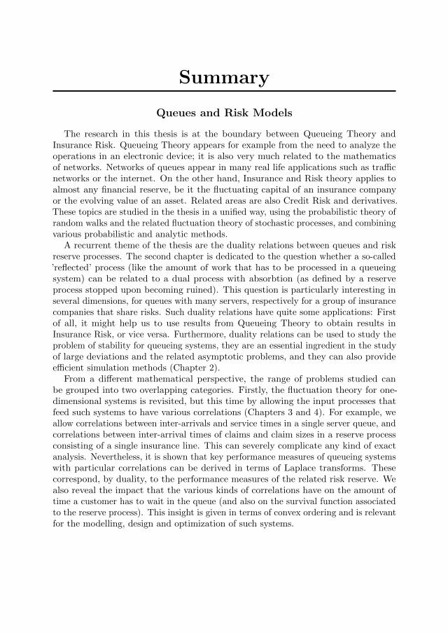
Summary

Queues and Risk Models

The research in this thesis is at the boundary between Queueing Theory andInsurance Risk. Queueing Theory appears for example from the need to analyze theoperations in an electronic device; it is also very much related to the mathematicsof networks. Networks of queues appear in many real life applications such as trafficnetworks or the internet. On the other hand, Insurance and Risk theory applies toalmost any financial reserve, be it the fluctuating capital of an insurance companyor the evolving value of an asset. Related areas are also Credit Risk and derivatives.These topics are studied in the thesis in a unified way, using the probabilistic theory ofrandom walks and the related fluctuation theory of stochastic processes, and combiningvarious probabilistic and analytic methods.

A recurrent theme of the thesis are the duality relations between queues and riskreserve processes. The second chapter is dedicated to the question whether a so-called’reflected’ process (like the amount of work that has to be processed in a queueingsystem) can be related to a dual process with absorbtion (as defined by a reserveprocess stopped upon becoming ruined). This question is particularly interesting inseveral dimensions, for queues with many servers, respectively for a group of insurancecompanies that share risks. Such duality relations have quite some applications: Firstof all, it might help us to use results from Queueing Theory to obtain results inInsurance Risk, or vice versa. Furthermore, duality relations can be used to study theproblem of stability for queueing systems, they are an essential ingredient in the studyof large deviations and the related asymptotic problems, and they can also provideefficient simulation methods (Chapter 2).

From a different mathematical perspective, the range of problems studied canbe grouped into two overlapping categories. Firstly, the fluctuation theory for one-dimensional systems is revisited, but this time by allowing the input processes thatfeed such systems to have various correlations (Chapters 3 and 4). For example, weallow correlations between inter-arrivals and service times in a single server queue, andcorrelations between inter-arrival times of claims and claim sizes in a reserve processconsisting of a single insurance line. This can severely complicate any kind of exactanalysis. Nevertheless, it is shown that key performance measures of queueing systemswith particular correlations can be derived in terms of Laplace transforms. Thesecorrespond, by duality, to the performance measures of the related risk reserve. Wealso reveal the impact that the various kinds of correlations have on the amount oftime a customer has to wait in the queue (and also on the survival function associatedto the reserve process). This insight is given in terms of convex ordering and is relevantfor the modelling, design and optimization of such systems.

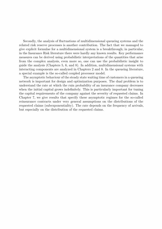
Secondly, the analysis of fluctuations of multidimensional queueing systems and therelated risk reserve processes is another contribution. The fact that we managed togive explicit formulae for a multidimensional system is a breakthrough; in particular,in the Insurance Risk literature there were hardly any known results. Key performancemeasures can be derived using probabilistic interpretations of the quantities that arisefrom the complex analysis, even more so, one can use the probabilistic insight toguide the analysis (Chapters 5, 6, and 8). In addition, multidimensional systems withinteracting components are analyzed in Chapters 2 and 8. In the queueing literature,a special example is the so-called coupled processor model.

The asymptotic behaviour of the steady state waiting time of customers in a queueingnetwork is important for design and optimization purposes. The dual problem is tounderstand the rate at which the ruin probability of an insurance company decreaseswhen the initial capital grows indefinitely. This is particularly important for tuningthe capital requirements of the company against the severity of requested claims. InChapter 7, we give results that specify these asymptotic regimes for the so-calledreinsurance contracts under very general assumptions on the distributions of therequested claims (subexponentiality). The rate depends on the frequency of arrivals,but especially on the distribution of the requested claims.

Curriculum Vitae

Emil Serban Badila was born in Targu-Mures on April 28, 1985. In 2004, he finishedsecondary education at Al. Papiu Ilarian high-school in Targu-Mures. Afterwards, hewent on to study Mathematics at the University of Bucharest. After graduation, hewas accepted on a scholarship for a Master program at Utrecht University, where hegraduated ’cum laude’ in 2010.

Having obtained the MSc degree, in 2011 he started a research project at EindhovenUniversity of Technology, under the supervision of Onno Boxma and Jacques Resing.The topic was at the boundary between Queueing Theory and Insurance Risk andthe current thesis is a compilation of most of the results obtained during the pastfour years. The research has led to the publication of several papers in internationaljournals. In addition, he has paid a couple of visits to the group of Hansjoerg Albrecherat the University of Lausanne, and at the Mathematical Institute of the University ofWroc law, for a collaboration with Zbigniew Palmowski and Tomasz Rolski.

He was also one of the organizers of the ’Queues and Risk Workshop’, in March2013. The research project is concluded with a thesis entitled ’Queues and Risk Models’which is to be defended on June 22, 2015.