Queueing Theory

Professor Stephen LawrenceLeeds School of Business

University of ColoradoBoulder, CO 80309-0419

2

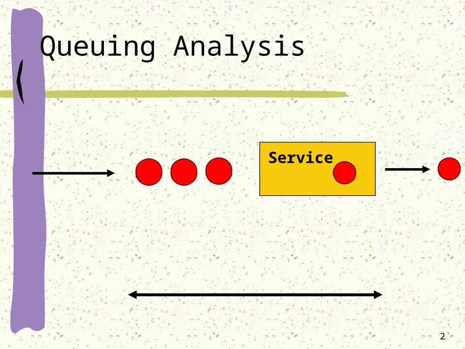
Service

Queuing Analysis

3

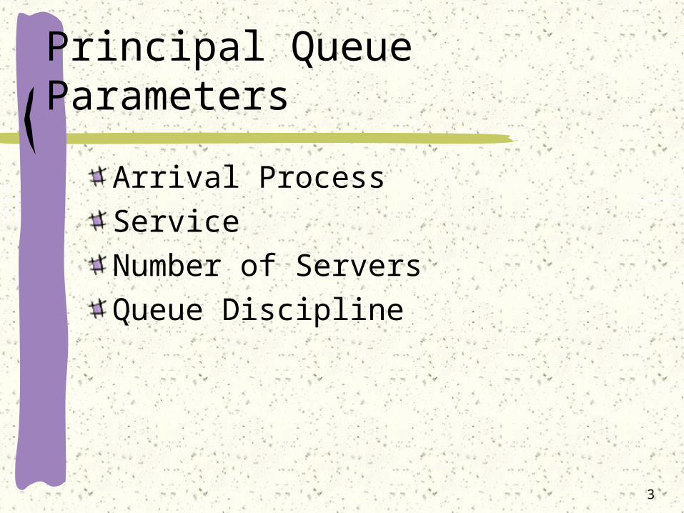
Principal Queue Parameters

Arrival ProcessServiceNumber of ServersQueue Discipline

4

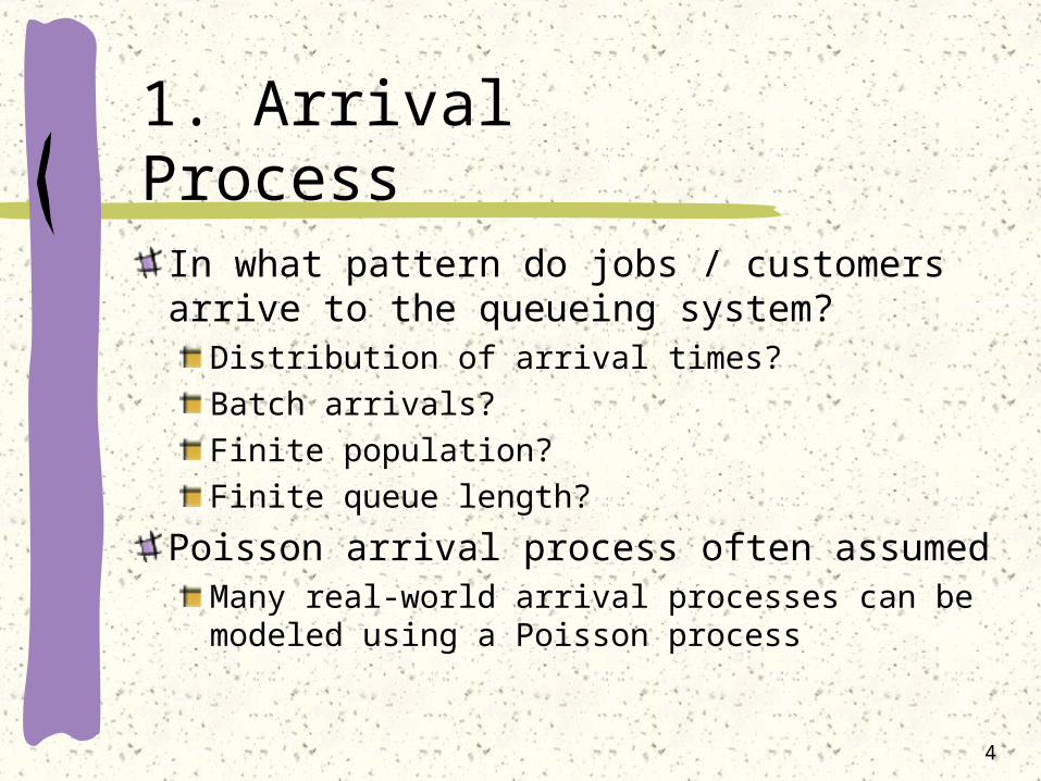
1. Arrival Process

In what pattern do jobs / customers arrive to the queueing system?

Distribution of arrival times?Batch arrivals?Finite population?Finite queue length?

Poisson arrival process often assumedMany real-world arrival processes can be modeled using a Poisson process

5

2. Service Process

How long does it take to service a job or customer?

Distribution of arrival times?Rework or repair?Service center (machine) breakdown?

Exponential service times often assumed

Works well for maintenance or unscheduled service situations

6

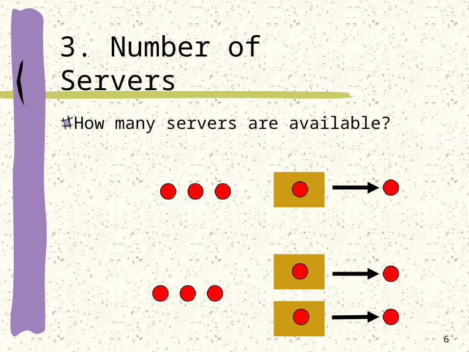
3. Number of Servers

How many servers are available?

7

4. Queue Discipline

How are jobs / customers selected from the queue for service?

First Come First Served (FCFS)Shortest Processing Time (SPT)Earliest Due Date (EDD)Priority (jobs are in different priority classes)

FCFS default assumption for most models

8

Queue Nomenclature

X / Y / k (Kendall notation)X = distribution of arrivals (iid)Y = distribution of service time (iid)

M = exponential (memoryless)Em = Erlang (parameter m)G = generalD = deterministic

k = number of servers

9

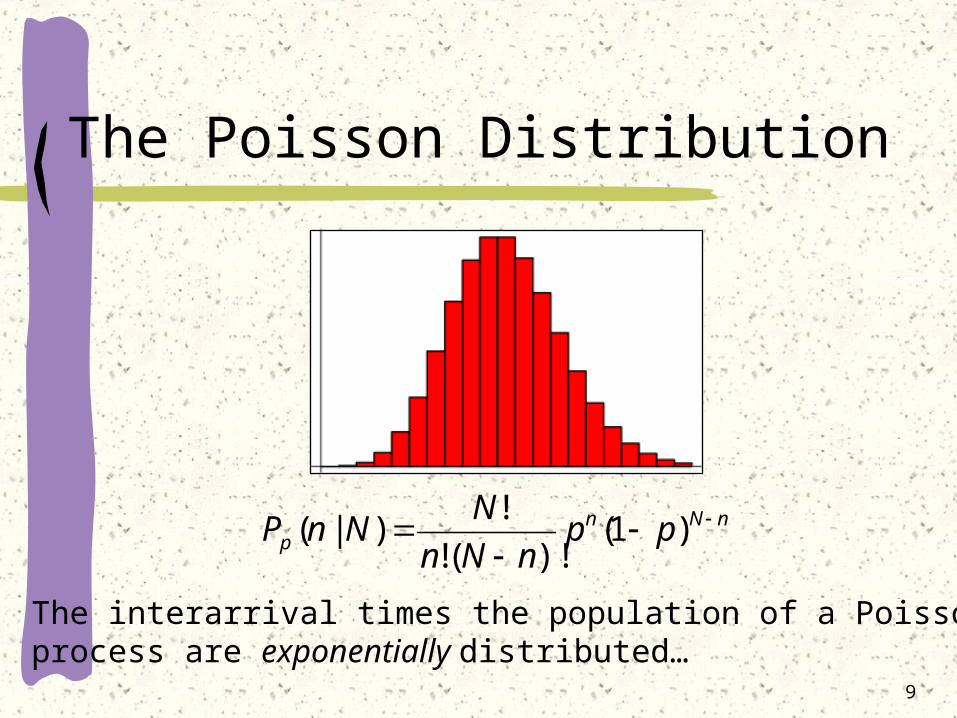
The Poisson Distribution

nNnp pp

nNn

NNnP

)1(

)!(!

!)|(

The interarrival times the population of a Poissonprocess are exponentially distributed…

10

Exponential Distribution

Simplest distributionSingle parameter (mean)Standard deviation fixed and equal to meanLacks memory

Remaining time exponentially distributed regardless of how much time has already passed

Interarrival times of a Poisson process are exponential

11

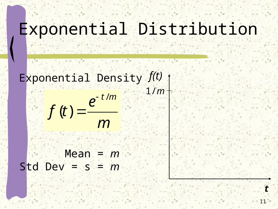
Exponential Distribution

m

etf

mt /

)(

Exponential Density

Mean = mStd Dev = s = m

f(t)1/m

t

M/M/1 Queues

13

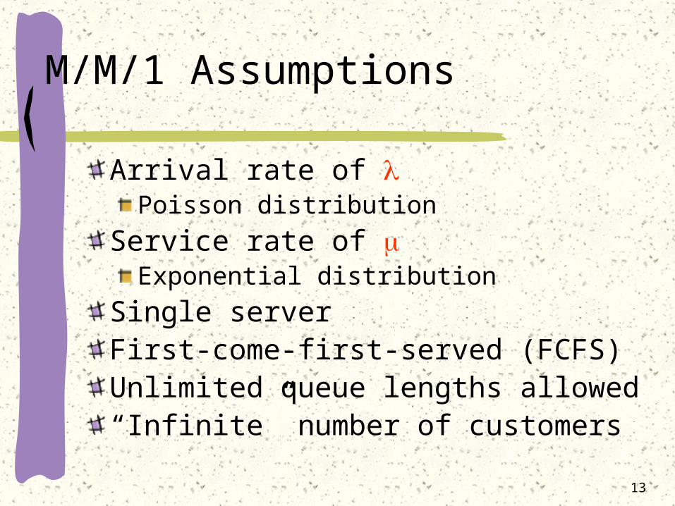
M/M/1 Assumptions

Arrival rate of Poisson distribution

Service rate of Exponential distribution

Single serverFirst-come-first-served (FCFS) Unlimited queue lengths allowed“Infinite” number of customers

14

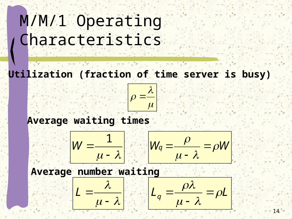
M/M/1 Operating Characteristics

Utilization (fraction of time server is busy)

Average waiting times

Average number waiting

1W WWq

L LLq

15

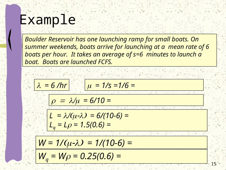
ExampleBoulder Reservoir has one launching ramp for small boats. On summer weekends, boats arrive for launching at a mean rate of 6 boats per hour. It takes an average of s=6 minutes to launch a boat. Boats are launched FCFS.

= 6 /hr

= 6/10 =

L = = 6/(10-6) = Lq = L = 1.5(0.6) =

W = 1/= 1/(10-6) =

Wq = W = 0.25(0.6) =

= 1/s =1/6 =

16

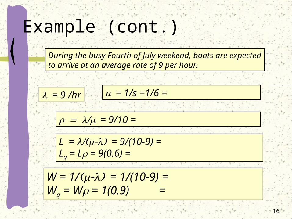
Example (cont.)

During the busy Fourth of July weekend, boats are expectedto arrive at an average rate of 9 per hour.

= 9 /hr = 1/s =1/6 =

= 9/10 =

L = = 9/(10-9) =Lq = L = 9(0.6) =

W = 1/= 1/(10-9) = Wq = W = 1(0.9) =

17

Another Example

The personal services officer of the Aspen Investors Bank interviews all potential customers to ascertain that they have sufficient net worth to become clients. Potential customers arrive at a rate of nine every 2 hours according to a Poisson distribution, and the officer spends an average of twelve minutes with each customer reviewing their portfolio with an exponential distribution. Determine the principal operating characteristics for this system.

18

Queue Simulation

Averages are deceptiveSimulation of M/M/1 queue shows the effect of varianceExcel spreadsheet queue simulation

Available on course website

19

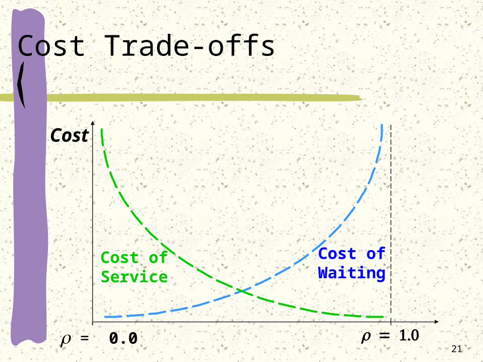
Managerial Implications

Low utilization levels provide better service levelsgreater flexibilitylower waiting costs (e.g., lost business)

High utilization levels provide better equipment and employee utilizationfewer idle periodslower production/service costs

Must trade off benefits of high utilization levels with benefits of flexibility and service

20

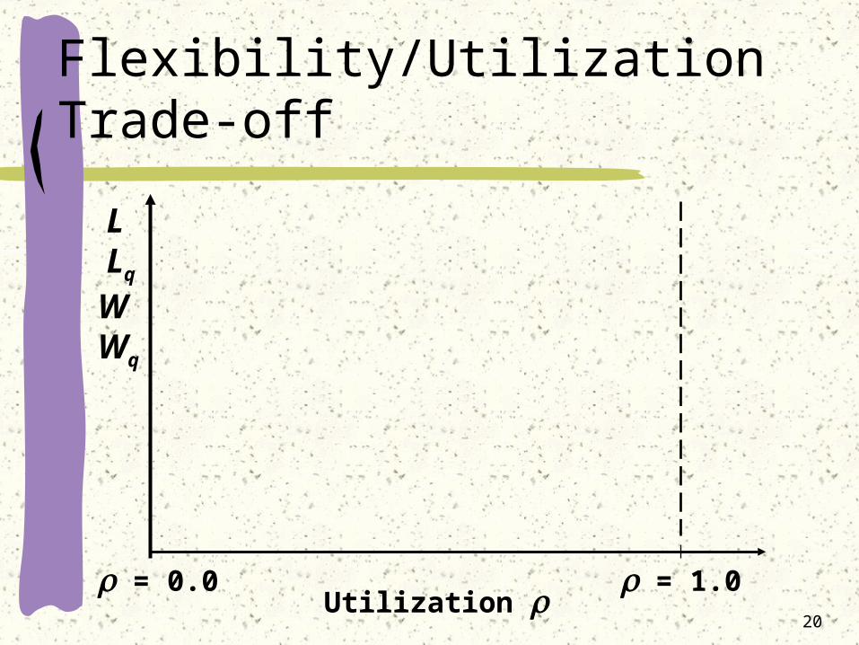
Flexibility/Utilization Trade-off

Utilization = 1.0= 0.0

L Lq

WWq

21

Cost Trade-offs

= 0.0

Cost

Cost ofWaiting

Cost ofService

G/G/k Queues

23

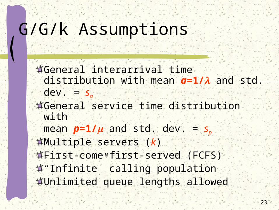
G/G/k Assumptions

General interarrival time distribution with mean a=1/ and std. dev. = sa

General service time distribution with mean p=1/ and std. dev. = sp

Multiple servers (k)First-come-first-served (FCFS)“Infinite” calling populationUnlimited queue lengths allowed

24

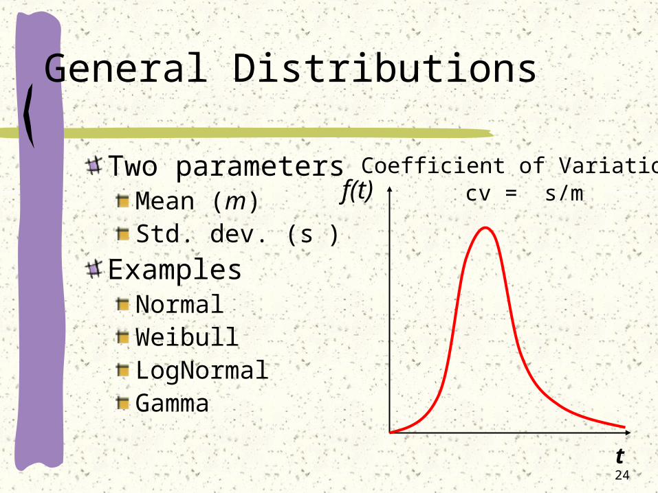
General Distributions

Two parametersMean (m)Std. dev. (s)

ExamplesNormalWeibullLogNormalGamma

f(t)

t

Coefficient of Variationcv = s/m

25

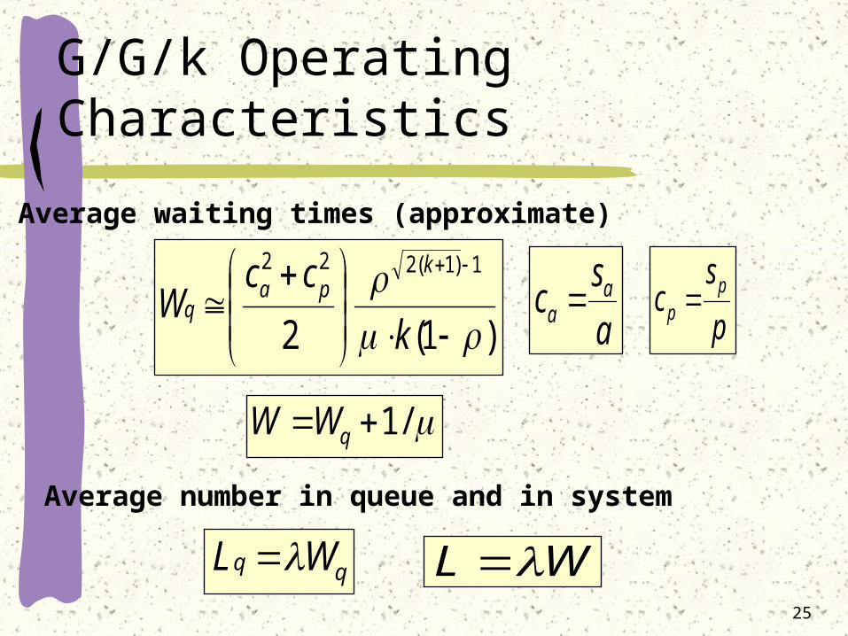
G/G/k Operating Characteristics

a

sc aa

Average waiting times (approximate)

Average number in queue and in system

)1(2

1)1(222

k

ccW

kpa

q

WL qq WL

/1 qWW

p

sc pp

26

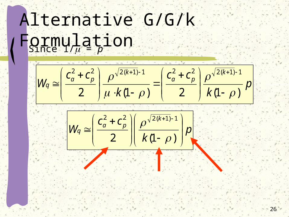
Alternative G/G/k Formulation

pk

cc

k

ccW

kpa

kpa

q)1(2)1(2

1)1(2221)1(222

pk

ccW

kpa

q

)1(2

1)1(222

Since 1/ = p

27

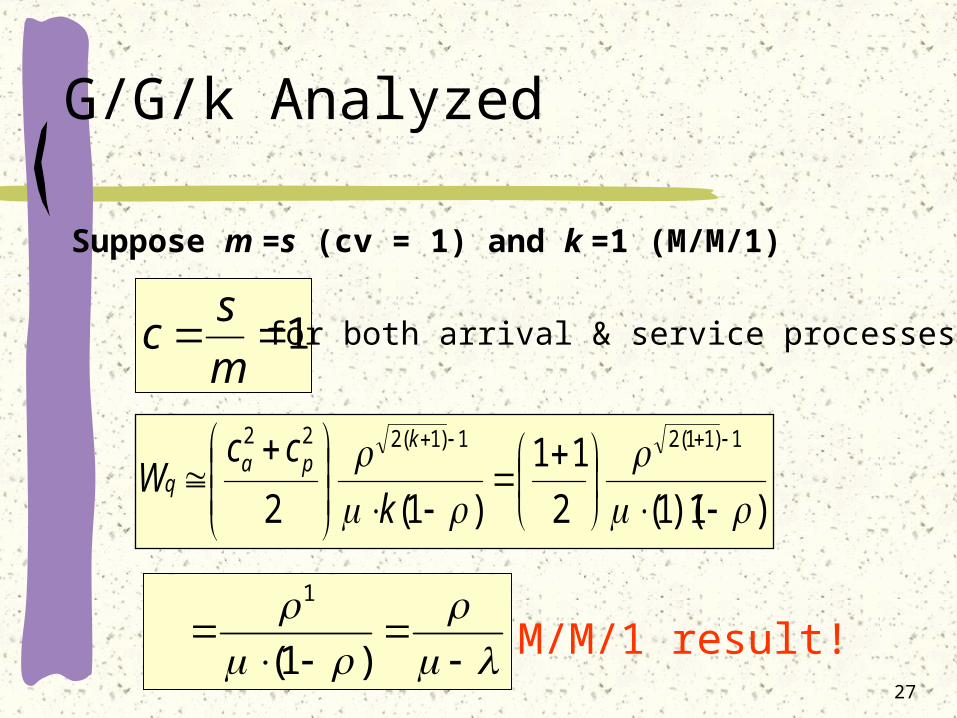
G/G/k Analyzed

Suppose m =s (cv = 1) and k =1 (M/M/1)

)1)(1(2

11

)1(2

1)11(21)1(222

k

ccW

kpa

q

1m

sc

)1(

1

M/M/1 result!

for both arrival & service processes

28

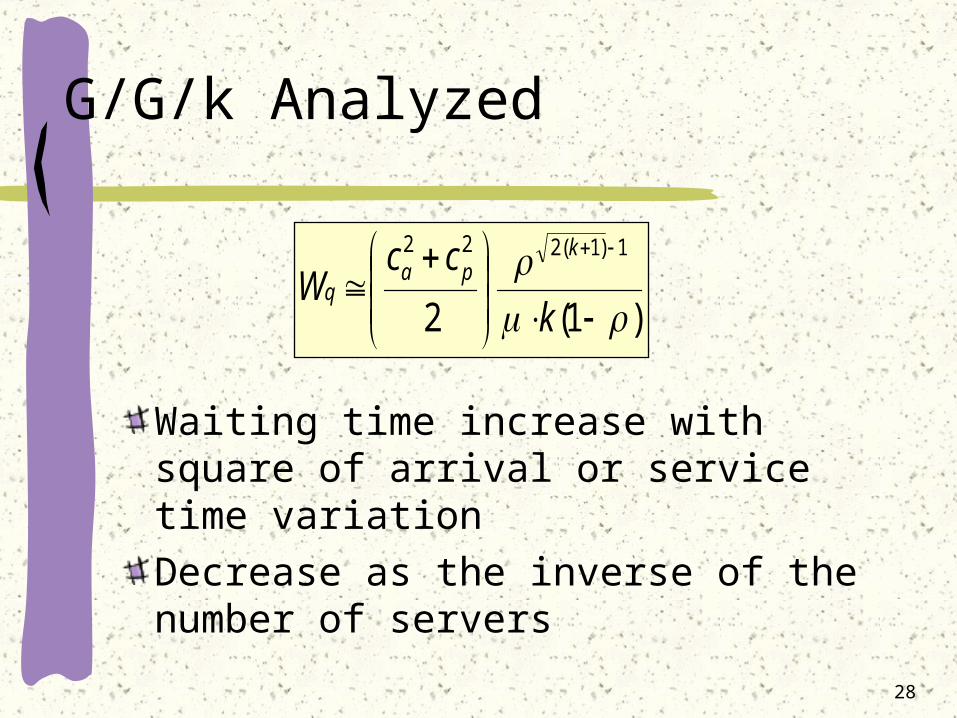
G/G/k Analyzed

Waiting time increase with square of arrival or service time variationDecrease as the inverse of the number of servers

)1(2

1)1(222

k

ccW

kpa

q

29

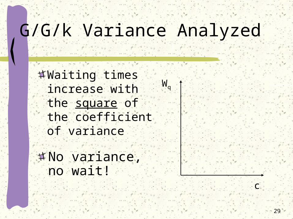
G/G/k Variance Analyzed

Waiting times increase with the square of the coefficient of varianceNo variance, no wait!

Wq

c

30

M/M/2 Example

The Boulder Parks staff is concerned about congestion during the busy Fourth of July weekend when boats are expected to arrive at an average rate of 9 per hour and take 6 minutes per boat to unload. Boulder is considering constructing a second temporary ramp next to the first to relieve congestion. What will be its effect?

31

Another G/G/k Example

Aspen Investors Bank wants to provide better service to its clients and is considering two alternatives:

1. Add a second personal services officer2. Install a computer system that will quickly

provide client information and reduce service time variance (service time standard deviation cut in half).

Recall that customers arrive at a rate of 4 per hour and are serviced at a rate of 5 per hour.

Other Queueing Models

33

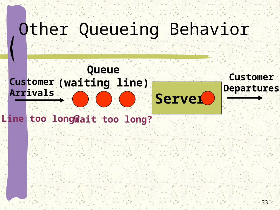
Other Queueing Behavior

Server

Queue(waiting line)Customer

Arrivals

CustomerDepartures

Wait too long?Line too long?

34

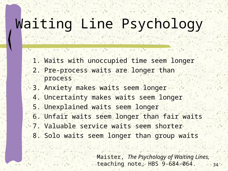
Waiting Line Psychology

1. Waits with unoccupied time seem longer2. Pre-process waits are longer than process3. Anxiety makes waits seem longer4. Uncertainty makes waits seem longer5. Unexplained waits seem longer6. Unfair waits seem longer than fair waits7. Valuable service waits seem shorter8. Solo waits seem longer than group waits

Maister, The Psychology of Waiting Lines, teaching note, HBS 9-684-064.

35

Queues and Simulation

Only simple queues can be mathematically analyzed“Real world” queues are often very complex

multiple servers, multiple queuesbalking, reneging, queue jumpingmachine breakdownsnetworks of queues, ...

Need to analyze, complex or not

Computer simulation !