Embed Size (px)
Citation preview


Queueing Modelling FundamentalsWith Applications in Communication Networks
Second Edition
Ng Chee-Hock and Soong Boon-HeeBoth of Nanyang Technological University, Singapore

Queueing Modelling Fundamentals

Queueing Modelling FundamentalsWith Applications in Communication Networks
Second Edition
Ng Chee-Hock and Soong Boon-HeeBoth of Nanyang Technological University, Singapore

Copyright © 2008 John Wiley & Sons Ltd, The Atrium, Southern Gate, Chichester, West Sussex PO19 8SQ, England
Telephone (+44) 1243 779777
Email (for orders and customer service enquiries): [email protected] our Home Page on www.wiley.com
All Rights Reserved. No part of this publication may be reproduced, stored in a retrieval system or transmitted in any form or by any means, electronic, mechanical, photocopying, recording, scanning or otherwise, except under the terms of the Copyright, Designs and Patents Act 1988 or under the terms of a licence issued by the Copyright Licensing Agency Ltd, 90 Tottenham Court Road, London W1T 4LP, UK, without the permission in writing of the Publisher. Requests to the Publisher should be addressed to the Permissions Department, John Wiley & Sons Ltd, The Atrium, Southern Gate, Chichester, West Sussex PO19 8SQ, England, or emailed to [email protected], or faxed to (+44) 1243 770620.
Designations used by companies to distinguish their products are often claimed as trademarks. All brand names and product names used in this book are trade names, service marks, trademarks or registered trademarks of their respective owners. The Publisher is not associated with any product or vendor mentioned in this book. All trademarks referred to in the text of this publication are the property of their respective owners.
This publication is designed to provide accurate and authoritative information in regard to the subject matter covered. It is sold on the understanding that the Publisher is not engaged in rendering professional services. If professional advice or other expert assistance is required, the services of a competent professional should be sought.
Other Wiley Editorial Offi ces
John Wiley & Sons Inc., 111 River Street, Hoboken, NJ 07030, USA
Jossey-Bass, 989 Market Street, San Francisco, CA 94103-1741, USA
Wiley-VCH Verlag GmbH, Boschstr. 12, D-69469 Weinheim, Germany
John Wiley & Sons Australia Ltd, 42 McDougall Street, Milton, Queensland 4064, Australia
John Wiley & Sons (Asia) Pte Ltd, 2 Clementi Loop #02-01, Jin Xing Distripark, Singapore 129809
John Wiley & Sons Canada Ltd, 6045 Freemont Blvd, Mississauga, ONT, L5R 4J3, Canada
Wiley also publishes its books in a variety of electronic formats. Some content that appears in print may not be available in electronic books.
Library of Congress Cataloging-in-Publication Data
Ng, Chee-Hock. Queueing modelling fundamentals with applications in communication networks / Chee-Hock Ng and Boon-Hee Song. – 2nd ed. p. cm. Includes bibliographical references and index. ISBN 978-0-470-51957-8 (cloth) 1. Queueing theory. 2. Telecommunication–Traffi c. I. Title. QA274.8.N48 2008 519.8′2 – dc22 2008002732
British Library Cataloguing in Publication Data
A catalogue record for this book is available from the British Library
ISBN 978-0-470-51957-8 (HB)
Typeset by SNP Best-set Typesetter Ltd., Hong KongPrinted and bound in Great Britain by TJ International, Padstow, Cornwall

To my wife, Joyce,and three adorable children, Sandra,
Shaun and Sarah, with love—NCH
To my wonderful wife, Buang Eng and children Jareth, Alec and Gayle,
for their understanding—SBH

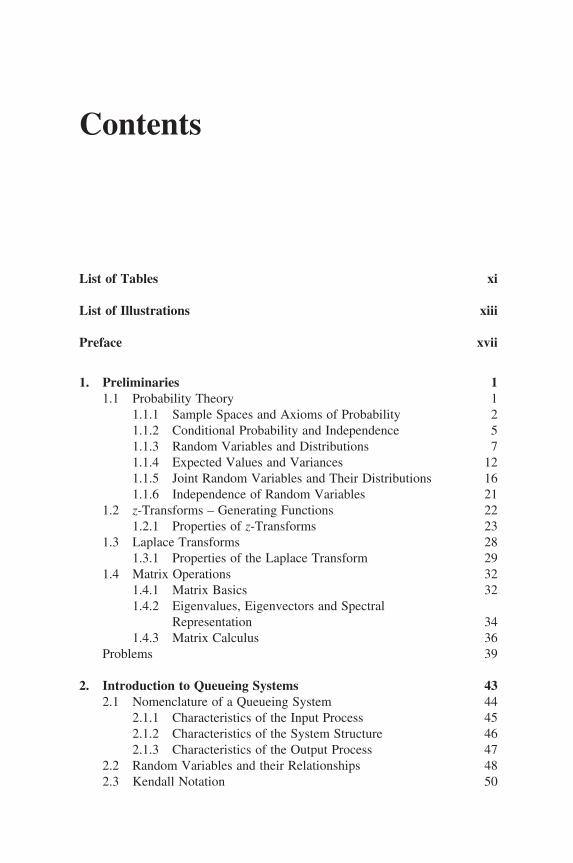
Contents
List of Tables xi
List of Illustrations xiii
Preface xvii
1. Preliminaries 11.1 Probability Theory 1
1.1.1 Sample Spaces and Axioms of Probability 21.1.2 Conditional Probability and Independence 51.1.3 Random Variables and Distributions 71.1.4 Expected Values and Variances 121.1.5 Joint Random Variables and Their Distributions 161.1.6 Independence of Random Variables 21
1.2 z-Transforms – Generating Functions 221.2.1 Properties of z-Transforms 23
1.3 Laplace Transforms 281.3.1 Properties of the Laplace Transform 29
1.4 Matrix Operations 321.4.1 Matrix Basics 321.4.2 Eigenvalues, Eigenvectors and Spectral Representation 34
1.4.3 Matrix Calculus 36Problems 39
2. Introduction to Queueing Systems 432.1 Nomenclature of a Queueing System 44
2.1.1 Characteristics of the Input Process 452.1.2 Characteristics of the System Structure 462.1.3 Characteristics of the Output Process 47
2.2 Random Variables and their Relationships 482.3 Kendall Notation 50
viii CONTENTS
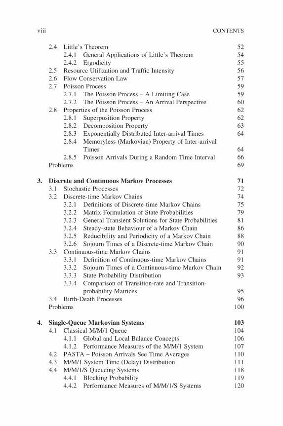
2.4 Little’s Theorem 522.4.1 General Applications of Little’s Theorem 542.4.2 Ergodicity 55
2.5 Resource Utilization and Traffi c Intensity 562.6 Flow Conservation Law 572.7 Poisson Process 59
2.7.1 The Poisson Process – A Limiting Case 592.7.2 The Poisson Process – An Arrival Perspective 60
2.8 Properties of the Poisson Process 622.8.1 Superposition Property 622.8.2 Decomposition Property 632.8.3 Exponentially Distributed Inter-arrival Times 642.8.4 Memoryless (Markovian) Property of Inter-arrival Times 642.8.5 Poisson Arrivals During a Random Time Interval 66
Problems 69
3. Discrete and Continuous Markov Processes 713.1 Stochastic Processes 723.2 Discrete-time Markov Chains 74
3.2.1 Defi nitions of Discrete-time Markov Chains 753.2.2 Matrix Formulation of State Probabilities 793.2.3 General Transient Solutions for State Probabilities 813.2.4 Steady-state Behaviour of a Markov Chain 863.2.5 Reducibility and Periodicity of a Markov Chain 883.2.6 Sojourn Times of a Discrete-time Markov Chain 90
3.3 Continuous-time Markov Chains 913.3.1 Defi nition of Continuous-time Markov Chains 913.3.2 Sojourn Times of a Continuous-time Markov Chain 923.3.3 State Probability Distribution 933.3.4 Comparison of Transition-rate and Transition- probability Matrices 95
3.4 Birth-Death Processes 96Problems 100
4. Single-Queue Markovian Systems 1034.1 Classical M/M/1 Queue 104
4.1.1 Global and Local Balance Concepts 1064.1.2 Performance Measures of the M/M/1 System 107
4.2 PASTA – Poisson Arrivals See Time Averages 1104.3 M/M/1 System Time (Delay) Distribution 1114.4 M/M/1/S Queueing Systems 118
4.4.1 Blocking Probability 1194.4.2 Performance Measures of M/M/1/S Systems 120
CONTENTS ix
4.5 Multi-server Systems – M/M/m 1244.5.1 Performance Measures of M/M/m Systems 1264.5.2 Waiting Time Distribution of M/M/m 127
4.6 Erlang’s Loss Queueing Systems – M/M/m/m Systems 1294.6.1 Performance Measures of the M/M/m/m 130
4.7 Engset’s Loss Systems 1314.7.1 Performance Measures of M/M/m/m with Finite Customer Population 133
4.8 Considerations for Applications of Queueing Models 134Problems 139
5. Semi-Markovian Queueing Systems 1415.1 The M/G/1 Queueing System 142
5.1.1 The Imbedded Markov-chain Approach 1425.1.2 Analysis of M/G/1 Queue Using Imbedded Markov-chain Approach 1435.1.3 Distribution of System State 1465.1.4 Distribution of System Time 147
5.2 The Residual Service Time Approach 1485.2.1 Performance Measures of M/G/1 150
5.3 M/G/1 with Service Vocations 1555.3.1 Performance Measures of M/G/1 with Service Vacations 156
5.4 Priority Queueing Systems 1585.4.1 M/G/1 Non-preemptive Priority Queueing 1585.4.2 Performance Measures of Non-preemptive Priority 1605.4.3 M/G/1 Pre-emptive Resume Priority Queueing 163
5.5 The G/M/1 Queueing System 1655.5.1 Performance Measures of GI/M/1 166
Problems 167
6. Open Queueing Networks 1696.1 Markovian Queries in Tandem 171
6.1.1 Analysis of Tandem Queues 1756.1.2 Burke’s Theorem 176
6.2 Applications of Tandem Queues in Data Networks 1786.3 Jackson Queueing Networks 181
6.3.1 Performance Measures for Open Networks 1866.3.2 Balance Equations 190
Problems 193
7. Closed Queueing Networks 1977.1 Jackson Closed Queueing Networks 1977.2 Steady-state Probability Distribution 199
x CONTENTS
7.3 Convolution Algorithm 2037.4 Performance Measures 2077.5 Mean Value Analysis 2107.6 Application of Closed Queueing Networks 213Problems 214
8. Markov-Modulated Arrival Process 2178.1 Markov-modulated Poisson Process (MMPP) 218
8.1.1 Defi nition and Model 2188.1.2 Superposition of MMPPs 2238.1.3 MMPP/G/1 2258.1.4 Applications of MMPP 226
8.2 Markov-modulated Bernoulli Process 2278.2.1 Source Model and Defi nition 2278.2.2 Superposition of N Identical MMBPs 2288.2.3 ΣMMBP/D/1 2298.2.4 Queue Length Solution 2318.2.5 Initial Conditions 233
8.3 Markov-modulated Fluid Flow 2338.3.1 Model and Queue Length Analysis 2338.3.2 Applications of Fluid Flow Model to ATM 236
8.4 Network Calculus 2368.4.1 System Description 2378.4.2 Input Traffi c Characterization – Arrival Curve 2398.4.3 System Characterization – Service Curve 2408.4.4 Min-Plus Algebra 241
9. Flow and Congestion Control 2439.1 Introduction 2439.2 Quality of Service 2459.3 Analysis of Sliding Window Flow Control Mechanisms 246
9.3.1 A Simple Virtual Circuit Model 2469.3.2 Sliding Window Model 247
9.4 Rate Based Adaptive Congestion Control 257
References 259
Index 265
List of Tables
Table 1.1 Means and variances of some common random variables 15Table 1.2 Some z-transform pairs 24Table 1.3 z-transforms for some of the discrete random variables 25Table 1.4 Some Laplace transform pairs 30Table 1.5 Laplace transforms for some probability functions 31Table 2.1 Random variables of a queueing system 49Table 3.1 Classifi cations of stochastic processes 73Table 3.2 A sample sequence of Bernoulli trials 75Table 3.3 Passengers’ traffi c demand 77Table 6.1 Traffi c load and routing information 191Table 6.2 Traffi c load and transmission speeds 192Table 6.3 Traffi c load and routing information for Figure 6.14 195Table 7.1 Normalization constants for Figure 7.3 when e1 = µ 205Table 7.2 Normalization constants for Figure 7.3 when e1 = 1–2 µ 206Table 7.3 Normalization constants for Figure 7.4 207Table 9.1 Main characteristics of each service and their application 245Table 9.2 Computation of G(n, m) 256Table 9.3 Normalized end-to-end throughput and delay 257

List of Illustrations
Figure 1.1 A closed loop of M queues 3Figure 1.2 N customers and M zeros, (N + M − 1) spaces 4Figure 1.3 Distribution function of a discrete random variable X 8Figure 1.4 Distribution function of a continuous RV 9Figure 1.5 The density function g(y) for I = 1 . . . 10 21Figure 1.6 A famous legendary puzzle 26Figure 1.7 Switches for Problem 6 39Figure 1.8 Communication network with 5 links 40Figure 2.1 Schematic diagram of a queneing system 44Figure 2.2 (a) Parallel servers 47Figure 2.2 (b) Serial servers 47Figure 2.3 A job-processing system 50Figure 2.4 An M/M1/m with fi nite customer population 51Figure 2.5 A closed queueing netwook model 51Figure 2.6 A sample pattern of arrival 53Figure 2.7 A queueing model of a switch 54Figure 2.8 Ensemble average of a process 56Figure 2.9 Flow Conservation Law 57Figure 2.10 Sample Poisson distributuon Function 62Figure 2.11 Superposition property 63Figure 2.12 Decomposition property 63Figure 2.13 Sample train arrival instants 65Figure 2.14 Conditional inter-arrival times 66Figure 2.15 Vulnerable period of a transmission 69Figure 2.16 A schematic diagram of a switching node 69Figure 3.1 State transition diagram 76Figure 3.2 State transition diagram for the lift example 77Figure 3.3 Transition diagram of two disjoined chains 88Figure 3.4 Transition diagram of two disjoined chains 89Figure 3.5 Periodic Markov chain 90Figure 3.6 Transition diagram of a birth-death process 96Figure 3.7 A two-state Markov process 98Figure 3.8 Probability distribution of a two-state Markov chain 99
Figure 3.9 Probability distribution of a Yule process 101Figure 3.10 A two-state discrete Markov chain 102Figure 4.1 An M/M/1 system 104Figure 4.2 Global balance concept 106Figure 4.3 Local balance concept 107Figure 4.4 Number of customers in the system M/M/1 109Figure 4.5 Transition diagram for Example 4.3 115Figure 4.6 Transition diagram for Example 4.4 117Figure 4.7 M/M/1/S transition diagram 118Figure 4.8 Blocking probability of a queueing 119Figure 4.9 System model for a multiplexer 123Figure 4.10 A multi-server system model 124Figure 4.11 M/M/m transition diagram 125Figure 4.12 A M/M/m/m system with fi nite customer population 132Figure 4.13 Transition diagram for M/M/m/m with fi nite customers 132Figure 4.14 A VDU-computer set up 138Figure 5.1 A M/G/1 queueing system 142Figure 5.2 Residual service time 148Figure 5.3 A sample pattern of the function r(t) 150Figure 5.4 A point-to-point setup 153Figure 5.5 Data exchange sequence 154Figure 5.6 A sample pattern of the function v(t) 156Figure 5.7 A multi-point computer terminal system 157Figure 5.8 M/G/1 non-preemptive priority system 159Figure 6.1 An example of open queueing networks 170Figure 6.2 An example of closed queueing networks 171Figure 6.3 Markovian queues in tandem 171Figure 6.4 State transition diagram of the tandem queues 173Figure 6.5 Queueing model for example 6-1 177Figure 6.6 A virtual circuit packet switching network 180Figure 6.7 Queueing model for a virtual circuit 180Figure 6.8 An open queueing network 182Figure 6.9 A queueing model for Example 6.3 188Figure 6.10 A multi-programming computer 189Figure 6.11 An open network of three queues 193Figure 6.12 CPU job scheduling system 193Figure 6.13 A schematic diagram of a switching node 194Figure 6.14 A 5-node message switching 194Figure 7.1 A closed network of three parallel queues 201Figure 7.2 Transition diagram for Example 7.2 202Figure 7.3 A closed network of three parallel queues 204Figure 7.4 A closed serial network 206Figure 7.5 A central server queueing system 213Figure 7.6 Queueing model for a virtual circuit 214
xiv LIST OF ILLUSTRATIONS
Figure 7.7 A closed network of three queues 215Figure 8.1 Markov-modulated Poisson process 218Figure 8.2 Superposition of MMPPs 224Figure 8.3 MMPP/G/1 225Figure 8.4 Interrupted Poisson Process model for a voice source 226Figure 8.5 An m-state MMPP model for voice sources 226Figure 8.6 A two-state MMBP 227Figure 8.7 A Markov-modulated fl uid model 234Figure 8.8 Schematic system view of a queue 237Figure 8.9 Arrivals and X(t) content 238Figure 8.10 Sample path of A(t) and D(t) 239Figure 8.11 Sample Arrival Curve 240Figure 9.1 Flow control design based on queueing networks 244Figure 9.2 Data network 246Figure 9.3 Simplifi ed model for a single virtual circuit 247Figure 9.4 Sliding window control model (closed queueing
network) 248Figure 9.5 Norton aggregation or decomposition of queueing
network 249Figure 9.6 State transition diagram 249Figure 9.7 Norton’s equivalent, cyclic queue network 251Figure 9.8 Delay throughput tradeoff curve for sliding window
fl ow control, M = 3, 4 and l → ∞ 252Figure 9.9 Packet-switching network transmission rates 255Figure 9.10 Typical closed network 255Figure 9.11 Sliding window closed network 256
LIST OF ILLUSTRATIONS xv

Preface
Welcome to the second edition of Queueing Modelling Fundamentals With Applications in Communication Networks. Since the publication of the fi rst edition by the fi rst author Ng Chee-Hock in 1996, this book has been adopted for use by several colleges and universities. It has also been used by many professional bodies and practitioners for self-study.
This second edition is a collaborative effort with the coming on board of a second author to further expand and enhance the contents of the fi rst edition. We have in this edition thoroughly revised all the chapters, updated examples and problems included in the text and added more worked examples and per-formance curves. We have included new materials/sections in several of the chapters, as well as a new Chapter 9 on ‘Flow and Congestion Control’ to further illustrate the various applications of queueing theory. A section on ‘Network Calculus’ is also added to Chapter 8 to introduce readers to a set of recent developments in queueing theory that enables deterministic bounds to be derived.
INTENDED AUDIENCE
Queueing theory is often taught at the senior level of an undergraduate pro-gramme or at the entry level of a postgraduate course in computer networking or engineering. It is often a prerequisite to some more advanced courses such as network design and capacity planning.
This book is intended as an introductory text on queueing modelling with examples on its applications in computer networking. It focuses on those queueing modelling techniques that are useful and applicable to the study of data networks and gives an in-depth insight into the underlying principles of isolated queueing systems as well as queueing networks. Although a great deal of effort is spent in discussing the models, their general applications are dem-onstrated through many worked examples.
It is the belief of the authors and experience learned from many years of teaching that students generally absorb the subject matter faster if the underly-ing concepts are demonstrated through examples. This book contains many
worked examples intended to supplement the teaching by illustrating the pos-sible applications of queueing theory. The inclusion of a large number of examples aims to strike a balance between theoretical treatment and practical applications.
This book assumes that students have a prerequisite knowledge on probabil-ity theory, transform theory and matrices. The mathematics used is appropriate for those students in computer networking and engineering. The detailed step-by-step derivation of queueing results makes it an excellent text for academic courses, as well as a text for self-study.
ORGANISATION OF THIS BOOK
This book is organised into nine chapters as outlined below:Chapter 1 refreshes the memory of students on those mathematical tools that
are necessary prerequisites. It highlights some important results that are crucial to the subsequent treatment of queueing systems.
Chapter 2 gives an anatomy of a queueing system, the various random vari-ables involved and the relationships between them. It takes a close look at a frequently-used arrival process – the Poisson process and its stochastic properties.
Chapter 3 introduces Markov processes that play a central role in the analysis of all the basic queueing systems – Markovian queueing systems.
Chapter 4 considers single-queue Markovian systems with worked examples of their applications. Emphasis is placed on the techniques used to derive the performance measures for those models that are widely used in computer com-munications and networking. An exhaustive listing of queueing models is not intended.
Chapter 5 looks at semi-Markovian systems, M/G/1 and its variants. G/M/1 is also mentioned briefl y to contrast the random observer property of these two apparently similar but conceptually very different systems.
Chapter 6 extends the analysis to the open queueing networks with a single class of customers. It begins with the treatment of two tandem queues and its limitations in applying the model to transmission channels in series, and sub-sequently introduces the Jackson queueing networks.
Chapter 7 completes the analysis of queueing networks by looking at other types of queueing networks – closed queueing networks. Again treatments are limited to the networks with a single class of customers.
Chapter 8 looks at some more exotic classes of arrival processes used to model those arrivals by correlation, namely the Markov-modulated Poisson process, the Markov-modulated Bernoulli process and the Markov-modulated fl uid fl ow. It also briefl y introduces a new paradigm of deterministic queueing called network calculus that allows deterministic bounds to be derived.
xviii PREFACE
Chapter 9 looks at the traffi c situation in communication networks where queueing networks can be applied to study the performance of fl ow control mechanisms. It also briefl y introduces the concept of sliding window and rate-based fl ow control mechanisms. Finally, several buffer allocation schemes are studied using Markovian systems that combat congested states.
ACKNOWLEDGEMENTS
This book would not have been possible without the support and encourage-ment of many people. We are indebted to Tan Chee Heng, a former colleague, for painstakingly going through the manuscripts of the fi rst edition.
The feedback and input of students who attended our course, who used this book as the course text, have also helped greatly in clarifying the topics and examples as well as improving the fl ow and presentation of materials in this edition of the book. Finally, we are grateful to Sarah Hinton, our Project Editor and Mark Hammond at John Wiley & Sons, Ltd for their enthusiastic help and patience.
PREFACE xix

1Preliminaries
Queueing theory is an intricate and yet highly practical fi eld of mathematical study that has vast applications in performance evaluation. It is a subject usually taught at the advanced stage of an undergraduate programme or the entry level of a postgraduate course in Computer Science or Engineering. To fully understand and grasp the essence of the subject, students need to have certain background knowledge of other related disciplines, such as probability theory and transform theory, as a prerequisite.
It is not the intention of this chapter to give a fi ne exposition of each of the related subjects but rather meant to serve as a refresher and highlight some basic concepts and important results in those related topics. These basic con-cepts and results are instrumental to the understanding of queueing theory that is outlined in the following chapters of the book. For more detailed treatment of each subject, students are directed to some excellent texts listed in the references.
1.1 PROBABILITY THEORY
In the study of a queueing system, we are presented with a very dynamic picture of events happening within the system in an apparently random fashion. Neither do we have any knowledge about when these events will occur nor are we able to predict their future developments with certainty. Mathematical models have to be built and probability distributions used to quantify certain parameters in order to render the analysis mathematically tractable. The
Queueing Modelling Fundamentals Second Edition Ng Chee-Hock and Soong Boon-Hee© 2008 John Wiley & Sons, Ltd
2 PRELIMINARIES
importance of probability theory in queueing analysis cannot be over-emphasized. It plays a central role as that of the limiting concept to calculus. The development of probability theory is closely related to describing ran-domly occurring events and has its roots in predicting the random outcome of playing games. We shall begin by defi ning the notion of an event and the sample space of a mathematical experiment which is supposed to mirror a real-life phenomenon.
1.1.1 Sample Spaces and Axioms of Probability
A sample space (Ω) of a random experiment is a collection of all the mutually exclusive and exhaustive simple outcomes of that experiment. A particular simple outcome (w) of an experiment is often referred to as a sample point. An event (E) is simply a subset of Ω and it contains a set of sample points that satisfy certain common criteria. For example, an event could be the even numbers in the toss of a dice and it contains those sample points [2], [4], [6]. We indicate that the outcome w is a sample point of an event E by writing w ∈ E. If an event E contains no sample points, then it is a null event and we write E = ∅. Two events E and F are said to be mutually exclusive if they have no sample points in common, or in other words the intersection of events E and F is a null event, i.e. E ∩ F = ∅.
There are several notions of probability. One of the classic defi nitions is based on the relative frequency approach in which the probability of an event E is the limiting value of the proportion of times that E was observed. That is
P EN
NN
E( ) =→∞
lim (1.1)
where NE is the number of times event E was observed and N is the total number of observations. Another one is the so-called axiomatic approach where the probability of an event E is taken to be a real-value function defi ned on the family of events of a sample space and satisfi es the following conditions:
Axioms of probability
(i) 0 ≤ P(E) ≤ 1 for any event in that experiment(ii) P(Ω) = 1(iii) If E and F are mutually exclusive events, i.e. E ∈ F = ∅, then P(E ∪ F)
= P(E) + P(F)
There are some fundamental results that can be deduced from this axiomatic defi nition of probability and we summarize them without proofs in the follow-ing propositions.
Proposition 1.1
(i) P(∅) = 0(ii) P(E
–) + P(E) = 1 for any event E in Ω, where E
– is the compliment of E.
(iii) P(E ∪ F) = P(E) + P(F) − P(E ∩ F), for any events E and F.(iv) P(E) ≤ P(F), if E ⊆ F.
(v) P E P E E E i ji
i i i j∪ = ∩ = ∅ ≠∑
i
( ), for , when .
Example 1.1
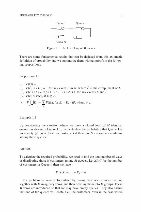
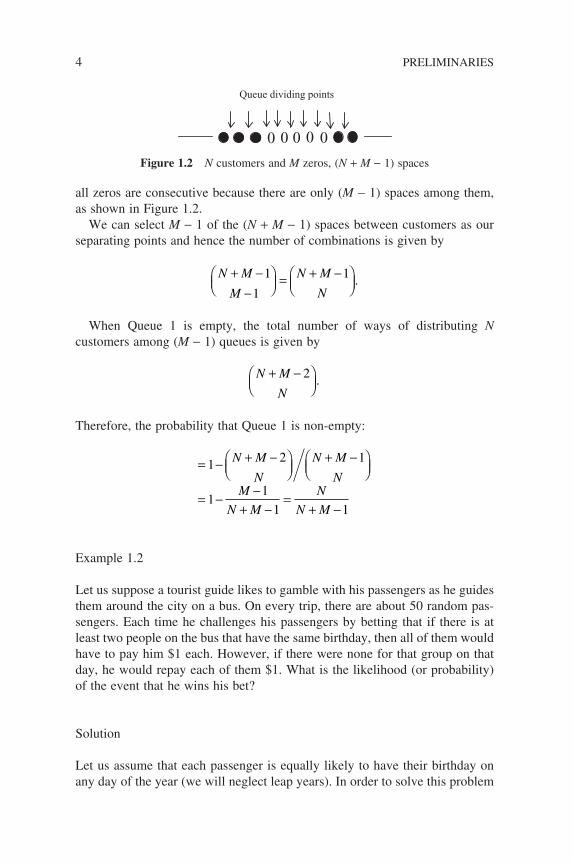
By considering the situation where we have a closed loop of M identical queues, as shown in Figure 1.1, then calculate the probability that Queue 1 is non-empty (it has at least one customer) if there are N customers circulating among these queues.
Solution
To calculate the required probability, we need to fi nd the total number of ways of distributing those N customers among M queues. Let Xi(>0) be the number of customers in Queue i, then we have
X1 + X2 + . . . + XM = N
The problem can now be formulated by having these N customers lined up together with M imaginary zeros, and then dividing them into M groups. These M zeros are introduced so that we may have empty queues. They also ensure that one of the queues will contain all the customers, even in the case where
Queue M
Queue kQueue 1
Figure 1.1 A closed loop of M queues
PROBABILITY THEORY 3
4 PRELIMINARIES
all zeros are consecutive because there are only (M − 1) spaces among them, as shown in Figure 1.2.
We can select M − 1 of the (N + M − 1) spaces between customers as our separating points and hence the number of combinations is given by
N M
M
N M
N
+ −−
= + −
1
1
1 .
When Queue 1 is empty, the total number of ways of distributing N customers among (M − 1) queues is given by
N M
N
+ −
2 .
Therefore, the probability that Queue 1 is non-empty:
= − + −
+ −
= −−
+ −=
+ −
1 2 1
11
1 1
N M
N
N M
NM
N M
N
N M
Example 1.2
Let us suppose a tourist guide likes to gamble with his passengers as he guides them around the city on a bus. On every trip, there are about 50 random pas-sengers. Each time he challenges his passengers by betting that if there is at least two people on the bus that have the same birthday, then all of them would have to pay him $1 each. However, if there were none for that group on that day, he would repay each of them $1. What is the likelihood (or probability) of the event that he wins his bet?
Solution
Let us assume that each passenger is equally likely to have their birthday on any day of the year (we will neglect leap years). In order to solve this problem
0 0 00 0
Queue dividing points
Figure 1.2 N customers and M zeros, (N + M − 1) spaces
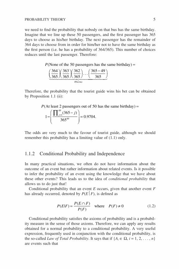
we need to fi nd the probability that nobody on that bus has the same birthday. Imagine that we line up these 50 passengers, and the fi rst passenger has 365 days to choose as his/her birthday. The next passenger has the remainder of 364 days to choose from in order for him/her not to have the same birthday as the fi rst person (i.e. he has a probability of 364/365). This number of choices reduces until the last passenger. Therefore:
P( )None of the passengers has the same birthday50
364
365
=
−
363
365
362
365
365 49
36549
. . .
terms
Therefore, the probability that the tourist guide wins his bet can be obtained by Proposition 1.1 (ii):
P( )At least 2 passengers out of has the same birthday50
1
=
−−−
==∏ jj
1
49
49
365
3650 9704
( ). .
The odds are very much to the favour of tourist guide, although we should remember this probability has a limiting value of (1.1) only.
1.1.2 Conditional Probability and Independence
In many practical situations, we often do not have information about the outcome of an event but rather information about related events. Is it possible to infer the probability of an event using the knowledge that we have about these other events? This leads us to the idea of conditional probability that allows us to do just that!
Conditional probability that an event E occurs, given that another event F has already occurred, denoted by P(EF), is defi ned as
P E FP E F
P FP F( | )
( )
( )( )=
∩≠where 0 (1.2)
Conditional probability satisfi es the axioms of probability and is a probabil-ity measure in the sense of those axioms. Therefore, we can apply any results obtained for a normal probability to a conditional probability. A very useful expression, frequently used in conjunction with the conditional probability, is the so-called Law of Total Probability. It says that if Ai ∈ Ω, i = 1, 2, . . . , n are events such that
PROBABILITY THEORY 5
6 PRELIMINARIES
(i) Ai ∩ Aj = ∅ if i ≠ j(ii) P(Ai) > 0
(iii) i
n
iA=
=1∪ Ω
then for any event E in the same sample space:
P E P E A P E A P Ai
n
ii
n
i i( ) ( ) ( | ) ( )= ∩ == =∑ ∑
1 1
(1.3)
This particular law is very useful for determining the probability of a complex event E by fi rst conditioning it on a set of simpler events Ai and then by summing up all the conditional probabilities. By substituting the expression (1.3) in the previous expression of conditional probability (1.2), we have the well-known Bayes’ formula:
P E FP E F
P F A P A
P F E P E
P F A P Ai
i ii
i i
( | )( )
( | ) ( )
( | ) ( )
( | ) ( )=
∩=
∑ ∑ (1.4)
Two events are said to be statistically independent if and only if
P(E ∩ F) = P(E)P(F).
From the defi nition of conditional probability, this also implies that
P E FP E F
P F
P E P F
P FP E( | )
( )
( )
( ) ( )
( )( )= ∩ = = (1.5)
Students should note that the statistical independence of two events E and F does not imply that they are mutually exclusive. If two events are mutually exclusive then their intersection is a null event and we have
P E FP E F
P FP F( | )
( )
( )( )= ∩ = ≠0 0where (1.6)
Example 1.3
Consider a switching node with three outgoing links A, B and C. Messages arriving at the node can be transmitted over one of them with equal probability. The three outgoing links are operating at different speeds and hence message transmission times are 1, 2 and 3 ms, respectively for A, B and C. Owing to
the difference in trucking routes, the probability of transmission errors are 0.2, 0.3 and 0.1, respectively for A, B and C. Calculate the probability of a message being transmitted correctly in 2 ms.
Solution
Denote the event that a message is transmitted correctly by F, then we are given
P(FA Link) = 1 − 0.2 = 0.8
P(FB Link) = 1 − 0.3 = 0.7
P(FC Link) = 1 − 0.1 = 0.9
The probability that a message being transmitted correctly in 2 ms is simply the event (F ∩ B), hence we have
P F B P F B P B( ) ( | ) ( )
.
∩ = ×
= × =0 71
3
7
30
1.1.3 Random Variables and Distributions
In many situations, we are interested in some numerical value that is associated with the outcomes of an experiment rather than the actual outcomes them-selves. For example, in an experiment of throwing two die, we may be inter-ested in the sum of the numbers (X) shown on the dice, say X = 5. Thus we are interested in a function which maps the outcomes onto some points or an interval on the real line. In this example, the outcomes are 2,3, 3,2, 1,4 and 4,1, and the point on the real line is 5.
This mapping (or function) that assigns a real value to each outcome in the sample space is called a random variable. If X is a random variable and x is a real number, we usually write X ≤ x to denote the event w ∈ Ω and X(w) ≤ x. There are basically two types of random variables; namely the dis-crete random variables and continuous random variables. If the mapping function assigns a real number, which is a point in a countable set of points on the real line, to an outcome then we have a discrete random variable. On the other hand, a continuous random variable takes on a real number which falls in an interval on the real line. In other words, a discrete random variable can assume at most a fi nite or a countable infi nite number of possible values and a continuous random variable can assume any value in an interval or intervals of real numbers.
PROBABILITY THEORY 7
8 PRELIMINARIES
A concept closely related to a random variable is its cumulative probabil-ity distribution function, or just distribution function (PDF). It is defi ned as
F x P X xP X x
X( ) [ ][ : ( ) ]
≡ ≤= ≤ω ω
(1.7)
For simplicity, we usually drop the subscript X when the random variable of the function referred to is clear in the context. Students should note that a distribution function completely describes a random variable, as all param-eters of interest can be derived from it. It can be shown from the basic axioms of probability that a distribution function possesses the following properties:
Proposition 1.2
(i) F is a non-negative and non-decreasing function, i.e. if x1 ≤ x2 then F(x1) ≤ F(x2)
(ii) F(+∞) = 1 & F(−∞) = 0(iii) F(b) − F(a) = P[a < X ≤ b]
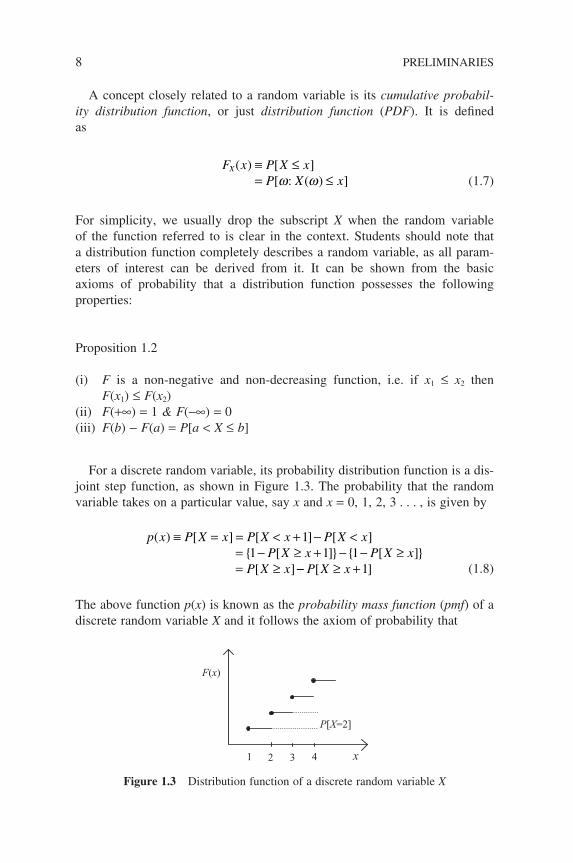
For a discrete random variable, its probability distribution function is a dis-joint step function, as shown in Figure 1.3. The probability that the random variable takes on a particular value, say x and x = 0, 1, 2, 3 . . . , is given by
p x P X x P X x P X x
P X x P X xP X x
( ) [ ] [ ] [ ] [ ] [ ]
[ ]
≡ = = < + − <= − ≥ + − − ≥= ≥
11 1 1
−− ≥ +P X x[ ]1
(1.8)
The above function p(x) is known as the probability mass function (pmf) of a discrete random variable X and it follows the axiom of probability that
F(x)
1 2
P[X=2]
3 4 x
Figure 1.3 Distribution function of a discrete random variable X
x
p x∑ =( ) 1 (1.9)
This probability mass function is a more convenient form to manipulate than the PDF for a discrete random variable.
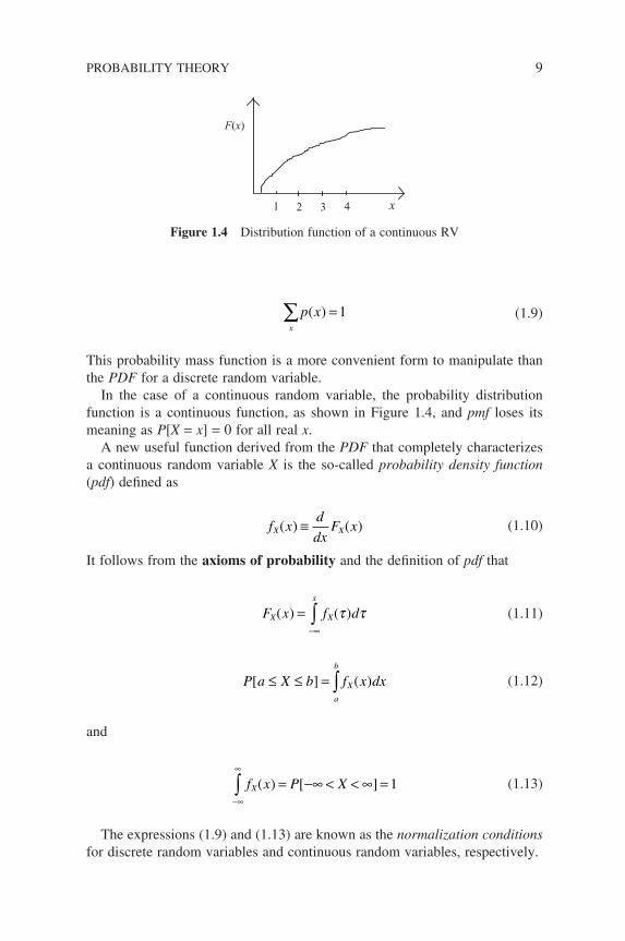
In the case of a continuous random variable, the probability distribution function is a continuous function, as shown in Figure 1.4, and pmf loses its meaning as P[X = x] = 0 for all real x.
A new useful function derived from the PDF that completely characterizes a continuous random variable X is the so-called probability density function (pdf) defi ned as
f xd
dxF xX X( ) ( )≡ (1.10)
It follows from the axioms of probability and the defi nition of pdf that
F x f dX
x
X( ) ( )=−∞∫ τ τ (1.11)
P a X b f x dxa
b
X[ ] ( )≤ ≤ = ∫ (1.12)
and
−∞
∞
∫ = −∞ < < ∞ =f x P XX( ) [ ] 1 (1.13)
The expressions (1.9) and (1.13) are known as the normalization conditions for discrete random variables and continuous random variables, respectively.
PROBABILITY THEORY 9
F(x)
1 2 3 4 x
Figure 1.4 Distribution function of a continuous RV
10 PRELIMINARIES
We list in this section some important discrete and continuous random vari-ables which we will encounter frequently in our subsequent studies of queueing models.
(i) Bernoulli random variableA Bernoulli trial is a random experiment with only two outcomes, ‘success’ and ‘failure’, with respective probabilities, p and q. A Bernoulli random vari-able X describes a Bernoulli trial and assumes only two values: 1 (for success) with probability p and 0 (for failure) with probability q:
P X p P X q p[ ] & [ ]= = = = = −1 0 1 (1.14)
(ii) Binomial random variableIf a Bernoulli trial is repeated k times then the random variable X that counts the number of successes in the k trials is called a binomial random variable with parameters k and p. The probability mass function of a binomial random variable is given by
B k n pn
kp q k n q pk n k( ; ) &, , , , . . . ,=
= = −− 0 1 2 1 (1.15)
(iii) Geometric random variableIn a sequence of independent Bernoulli trials, the random variable X that counts the number of trials up to and including the fi rst success is called a geometric random variable with the following pmf:
P X k p p kk[ ] ( )= = − = ∞−1 1 21 , , . . . (1.16)
(iv) Poisson random variableA random variable X is said to be Poisson random variable with parameter l if it has the following mass function:
P X kk
e kk
[ ]!
= = =−λ λ 0 1 2, , , . . . (1.17)
Students should note that in subsequent chapters, the Poisson mass function is written as
P X kt
ke k
kt[ ]
( )
!= = ′ =− ′λ λ 0 1 2, , , . . . (1.18)
Here, the l in expression (1.17) is equal to the l′t in expression (1.18).
(v) Continuous uniform random variableA continuous random variable X with its probabilities distributed uniformly over an interval (a, b) is said to be a uniform random variable and its density function is given by
f x b aa x b
otherwise( ) = −
< <
1
0 (1.19)
The corresponding distribution function can be easily calculated by using expression (1.11) as
F x
x a
x a
b aa x b
x b
( ) =
<−−
≤ <
≥
0
1
(1.20)
(vi) Exponential random variableA continuous random variable X is an exponential random variable with parameter l > 0, if its density function is defi ned by
f xe x
x
x
( ) =>≤
−λ λ 0
0 0 (1.21)
The distribution function is then given by
F xe x
x
x
( ) =− >
≤
−1 0
0 0
λ λ
(1.22)
(vii) Gamma random variableA continuous random variable X is said to have a gamma distribution with parameters a > 0 and l > 0, if its density function is given by
f x
x ex
x
x
( )( )
( )=>
≤
− −λα
α α λ1
0
0 0
Γ (1.23)
where Γ(a) is the gamma function defi ned by
Γ( )α αα= >∞
− −∫0
1 0x e dxx (1.24)
PROBABILITY THEORY 11
12 PRELIMINARIES
There are certain nice properties about gamma functions, such as
Γ Γ
Γ Γ
( ) ( ) ( ) ( )!
( ) ( )
k k k k n a positive eger
a
= − − = − =
= − >
1 1 1
1 0
α
α α α α
int
rreal number
(1.25)
(viii) Erlang-k or k-stage Erlang Random VariableThis is a special case of the gamma random variable when a (=k) is a positive integer. Its density function is given by
f x
x
ke x
x
k kx
( )
( )
( )!= −>
≤
−−λ λ
1
10
0 0
(1.26)
(ix) Normal (Gaussian) Random VariableA frequently encountered continuous random variable is the Gaussian or Normal with the parameters of m (mean) and sX (standard deviation). It has a density function given by
f x eX
X
x X( ) ( ) /= − −1
2 2
22 2
πσµ σ (1.27)
The normal distribution is often denoted in a short form as N(m, s 2X).Most of the examples above can be roughly separated into either continuous
or discrete random variables. A discrete random variable can take on only a fi nite number of values in any fi nite observations (e.g. the number of heads obtained in throwing 2 independent coins). On the other hand, a continuous random variable can take on any value in the observation interval (e.g. the time duration of telephone calls). However, samples may exist, as we shall see later, where the random variable of interest is a mixed random variable, i.e. they have both continuous and discrete portions. For example, the waiting time distribu-tion function of a queue in Section 4.3 can be shown as
F t e t
tW
t( ) ( )
.
( )= − ≥= <
− −1 0
0 0
1ρ µ ρ
This has a discrete portion that has a jump at t = 0 but with a continuous portion elsewhere.
1.1.4 Expected Values and Variances
As discussed in Section 1.1.3, the distribution function or pmf (pdf, in the case of continuous random variables) provides a complete description of a random
variable. However, we are also often interested in certain measures which sum-marize the properties of a random variable succinctly. In fact, often these are the only parameters that we can observe about a random variable in real-life problems.
The most important and useful measures of a random variable X are its expected value1 E[X] and variance Var[X]. The expected value is also known as the mean value or average value. It gives the average value taken by a random variable and is defi ned as
E X kP X kk
[ ] [ ]= ==
∞
∑0
for discrete variables (1.28)
and E X xf x dx[ ] ( )=∞
∫0
for continuous variables (1.29)
The variance is given by the following expressions. It measures the disper-sion of a random variable X about its mean E[X]:
σ 2
2
2 2
== −= −
Var XE X E XE X E X
[ ][( [ ]) ][ ] ( [ ])
for discrete variables (1.30)
σ 2
0
2
0
2
0 0
2
=
= −
= − +
∞
∞ ∞
∫
∫ ∫
Var X
x E X f x d x
x f x dx E X xf x dx
[ ]
( [ ]) ( )
( ) [ ] ( )∞∞
∫= −
f x dx
E X E X
( )
[ ] ( [ ])2 2
(1.31)
s refers to the square root of the variance and is given the special name of standard deviation.
Example 1.4
For a discrete random variable X, show that its expected value is also given by
E X P X kk
[ ] [ ]= >=
∞
∑0
PROBABILITY THEORY 13
for continuous variables
1 For simplicity, we assume here that the random variables are non-negative.
14 PRELIMINARIES
Solution
By defi nition, the expected value of X is given by
E X kP X k k P X k P X kk k
[ ] [ ] [ ] [ ]= = = ≥ − ≥ +=
∞
=
∞
∑ ∑0 0
1 (see (1.8))
= ≥ − ≥ + ≥ − ≥+ ≥ − ≥ + ≥ −P X X P X P X
P X P X P X P X[ ] [ ] [ ] [ ]
[ ] [ ] [ ] [1 2 2 2 2 3
3 3 3 4 4 4 4 ≥≥ +
= ≥ = >=
∞
=
∞
∑ ∑5
1 0
]
[ ] [ ]
. . .
k k
P X k P X k
Example 1.5
Calculate the expected values for the Binomial and Poisson random variables.
Solution
1. Binomial random variable
E X kn
kp p
npn
kp P
k
nk n k
k
nk
[ ] ( )
( )
=
−
=−−
−
=
−
=
−
∑
∑1
1
1
1
1
11 nn k
j
nj n jnp
n
jp p
np
−
=
− −=−
−
=
∑0
111( )( )
2. Poisson random variable
E X kk
e
ek
e e
k
k
k
k
[ ]!
( )( )
( )!( )
=
=−
==
=
∞−
−
=
∞ −
−
∑
∑0
1
1
1
λ
λ λ
λλ
λ
λ
λ λ
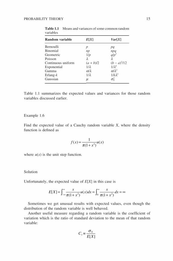
Table 1.1 summarizes the expected values and variances for those random variables discussed earlier.
Example 1.6
Find the expected value of a Cauchy random variable X, where the density function is defi ned as
f xx
u x( )( )
( )=+1
1 2π
where u(x) is the unit step function.
Solution
Unfortunately, the expected value of E[X] in this case is
E Xx
xu x dx
x
xdx[ ]
( )( )
( )=
+=
+= ∞
−∞
∞ ∞
∫ ∫π π1 12 0 2
Sometimes we get unusual results with expected values, even though the distribution of the random variable is well behaved.
Another useful measure regarding a random variable is the coeffi cient of variation which is the ratio of standard deviation to the mean of that random variable:
CE X
xX≡ σ
[ ]
PROBABILITY THEORY 15
Table 1.1 Means and variances of some common random variables
Random variable E[X] Var[X]
Bernoulli p pqBinomial np npqGeometric 1/p q/p2
Poisson l lContinuous uniform (a + b)/2 (b − a)2/12Exponential 1/l 1/l2
Gamma a/l a/l2
Erlang-k 1/l 1/kl2
Gaussian m s 2X
16 PRELIMINARIES
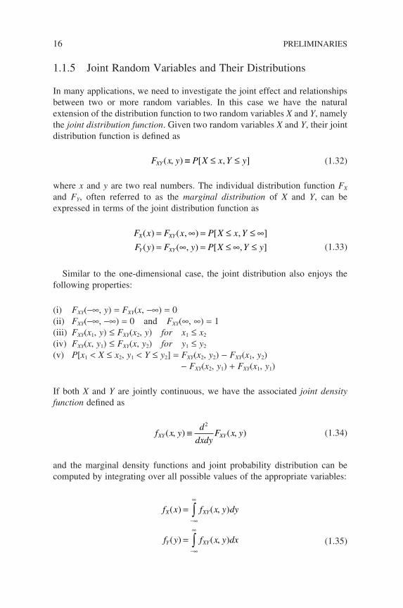
1.1.5 Joint Random Variables and Their Distributions
In many applications, we need to investigate the joint effect and relationships between two or more random variables. In this case we have the natural extension of the distribution function to two random variables X and Y, namely the joint distribution function. Given two random variables X and Y, their joint distribution function is defi ned as
F x y P X x Y yXY( ) [ ], ,≡ ≤ ≤ (1.32)
where x and y are two real numbers. The individual distribution function FX and FY, often referred to as the marginal distribution of X and Y, can be expressed in terms of the joint distribution function as
F x F x P X x Y
F y F y P X Y yX XY
Y XY
( ) ( [ ]
( ) ( ) [ ]
= ∞ = ≤ ≤ ∞= ∞ = ≤ ∞ ≤
, ) ,
, ,
(1.33)
Similar to the one-dimensional case, the joint distribution also enjoys the following properties:
(i) FXY(−∞, y) = FXY(x, −∞) = 0(ii) FXY(−∞, −∞) = 0 and FXY(∞, ∞) = 1(iii) FXY(x1, y) ≤ FXY(x2, y) for x1 ≤ x2
(iv) FXY(x, y1) ≤ FXY(x, y2) for y1 ≤ y2
(v) P[x1 < X ≤ x2, y1 < Y ≤ y2] = FXY(x2, y2) − FXY(x1, y2) − FXY(x2, y1) + FXY(x1, y1)
If both X and Y are jointly continuous, we have the associated joint density function defi ned as
f x yd
dxdyF x yXY XY( ) ( ), ,≡
2
(1.34)
and the marginal density functions and joint probability distribution can be computed by integrating over all possible values of the appropriate variables:
f x f x y dy
f y f x y dx
X XY
Y XY
( ) ( )
( ) ( )
=
=
−∞
∞
−∞
∞
∫
∫
,
,
(1.35)
F x y f u v dudvXY
x y
XY( ) ( ), ,=−∞ −∞∫ ∫
If both are jointly discrete then we have the joint probability mass function defi ned as
p x y P X x Y y( ) [ ], ,≡ = = (1.36)
and the corresponding marginal mass functions can be computed as
P X x p x y
P Y y p x y
y
x
[ ] ( )
[ ] ( )
= =
= =
∑
∑
,
,
(1.37)
With the defi nitions of joint distribution and density function in place, we are now in a position to extend the notion of statistical independence to two random variables. Basically, two random variables X and Y are said to be statistically independent if the events x ∈ E and y ∈ F are inde-pendent, i.e.:
P[x ∈ E, y ∈ F ] = P[x ∈ E ] · P[y ∈ F ]
From the above expression, it can be deduced that X and Y are statistically independent if any of the following relationships hold:
• FXY (x, y) = FX (x) · FY (y)• fXY (x, y) = fX (x) · fY (y) if both are jointly continuous• P[x = x, Y = y] = P[X = x] · P[Y = y] if both are jointly discrete
We summarize below some of the properties pertaining to the relationships between two random variables. In the following, X and Y are two independent random variables defi ned on the same sample space, c is a constant and g and h are two arbitrary real functions.
(i) Convolution Property If Z = X + Y, then
• if X and Y are jointly discrete
P Z k P X i P Y j P X i P Y k ii j k i
k
[ ] [ ] [ ] [ ] [ ]= = = = = = = −+ = =∑ ∑
0
(1.38)
PROBABILITY THEORY 17
18 PRELIMINARIES
• if X and Y are jointly continuous
f z f x f z x dx f z y f y dy
f x f y
Z X Y X Y
X Y
( ) ( ) ( ) ( ) ( )
( ) ( )
= − = −
= ⊗
∞ ∞
∫ ∫0 0
(1.39)
where ⊗ denotes the convolution operator.
(ii) E[cX ] = cE[X ](iii) E[X + Y ] = E[X ] + E[Y ](iv) E[g(X)h(Y )] = E[g(X )] · E[h(Y )] if X and Y are independent(v) Var[cX ] = c2Var[X ](vi) Var[X + Y ] = Var[X ] + Var[Y ] if X and Y are independent(vi) Var[X ] = E[X2] − (E[X ])2
Example 1.7: Random sum of random variables
Consider the voice packetization process during a teleconferencing session, where voice signals are packetized at a teleconferencing station before being transmitted to the other party over a communication network in packet form. If the number (N) of voice signals generated during a session is a random vari-able with mean E(N), and a voice signal can be digitized into X packets, fi nd the mean and variance of the number of packets generated during a tele-conferencing session, assuming that these voice signals are identically distributed.
Solution
Denote the number of packets for each voice signal as Xi and the total number of packets generated during a session as T, then we have
T = X1 + X2 + . . . + XN
To calculate the expected value, we fi rst condition it on the fact that N = k and then use the total probability theorem to sum up the probability. That is:
E T E T N k P N k
kE X P N k
E X E N
i
N
i
N
[ ] [ | ] [ ]
[ ] [ ]
[ ] [ ]
= = =
= =
=
=
=
∑
∑1
1
To compute the variance of T, we fi rst compute E[T2]:
E T N k Var T N k E T N kkVar X k E X
[ | ] [ | ] ( [ | ])[ ] ( [ ])
2 2
2 2
= = = + == +
and hence we can obtain
E T kVar X k E X P N k
Var X E N E N E Xk
N
[ ] ( [ ] ( [ ]) ) [ ]
[ ] [ ] [ ]( [ ]
2
1
2 2
2
= + =
= +=
∑))2
Finally:
Var T E T E TVar X E N E N E X E X E N
[ ] [ ] ( [ ])[ ] [ ] [ ]( [ ]) ( [ ]) ( [ ])
= −= + −
2 2
2 2 2 22
2= +Var X E N E X Var N[ ] [ ] ( [ ]) [ ]
Example 1.8
Consider two packet arrival streams to a switching node, one from a voice source and the other from a data source. Let X be the number of time slots until a voice packet arrives and Y the number of time slots till a data packet arrives. If X and Y are geometrically distributed with parameters p and q respectively, fi nd the distribution of the time (in terms of time slots) until a packet arrives at the node.
Solution
Let Z be the time until a packet arrives at the node, then Z = min(X, Y ) and we have
P Z k P X k P Y k
F k F k F kZ X Y
[ ] [ ] [ ]
( ) ( ) ( )
> = > >
− = − −1 1 1
but
F k p p pp
p
p
Xj
jk
k
( ) ( )( )
( )
( )
= − = − −− −
= − −=
∞−∑
1
111 1
1 1
1 1
PROBABILITY THEORY 19
20 PRELIMINARIES
Similarly
FY(k) = 1 − (1 − q)k
Therefore, we obtain
F k p qp q
Zk k
k
( ) ( ) ( )[( )( )]
= − − −= − − −
1 1 11 1 1
Theorem 1.1
Suppose a random variable Y is a function of a fi nite number of independent random variables Xi, with arbitrary known probability density functions (pdf). If
Y Xi==∑i
n
1
then the pdf of Y is given by the density function:
g y f x f x f x f xY X X X Xn n( ) ( ) ( ) ( ) ( )= ⊗ ⊗ ⊗1 1 2 2 3 3 . . . (1.40)
The keen observer might note that this result is a general extension of expres-sion (1.39). Fortunately the convolution of density functions can be easily handled by transforms (z or Laplace).
Example 1.9
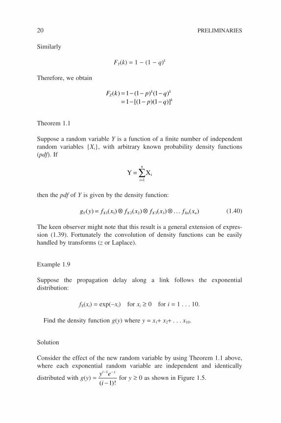
Suppose the propagation delay along a link follows the exponential distribution:
fX(xi) = exp(−xi) for xi ≥ 0 for i = 1 . . . 10.
Find the density function g(y) where y = x1+ x2+ . . . x10.
Solution
Consider the effect of the new random variable by using Theorem 1.1 above, where each exponential random variable are independent and identically
distributed with g(y) = y e
i
i y− −
−
1
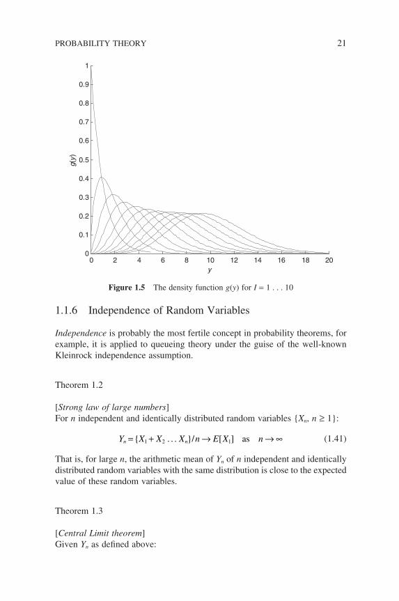
1( )! for y ≥ 0 as shown in Figure 1.5.
1.1.6 Independence of Random Variables
Independence is probably the most fertile concept in probability theorems, for example, it is applied to queueing theory under the guise of the well-known Kleinrock independence assumption.
Theorem 1.2
[Strong law of large numbers]For n independent and identically distributed random variables Xn, n ≥ 1:
Y X X X n E X nn n= + → → ∞ [ ]1 2 1. . . / as (1.41)
That is, for large n, the arithmetic mean of Yn of n independent and identically distributed random variables with the same distribution is close to the expected value of these random variables.
Theorem 1.3
[Central Limit theorem]Given Yn as defi ned above:
PROBABILITY THEORY 21
0 2 4 6 8 10 12 14 16 18 200
0.1
0.2
0.3
0.4
0.5
0.6
0.7
0.8
0.9
1
y
g(y)
Figure 1.5 The density function g(y) for I = 1 . . . 10
22 PRELIMINARIES
[ ] ( )Y E X n N nn − ≈ >>120 1, forσ (1.42)
where N(0,s 2) denotes the random variable with mean zero and variance s 2 of each Xn.
The theorem says that the difference between the arithmetic mean of Yn and the expected value E[X1] is a Gaussian distributed random variable divided by
n for large n.
1.2 z-TRANSFORMS – GENERATING FUNCTIONS
If we have a sequence of numbers f0, f1, f2, . . . fk . . ., possibly infi nitely long, it is often desirable to compress it into a single function – a closed-form expres-sion that would facilitate arithmetic manipulations and mathematical proofi ng operations. This process of converting a sequence of numbers into a single function is called the z-transformation, and the resultant function is called the z-transform of the original sequence of numbers. The z-transform is commonly known as the generating function in probability theory.
The z-transform of a sequence is defi ned as
F z f zk
kk( ) ≡
=
∞
∑0
(1.43)
where zk can be considered as a ‘tag’ on each term in the sequence and hence its position in that sequence is uniquely identifi ed should the sequence need to be recovered. The z-transform F(z) of a sequence exists so long as the sequence grows slower than ak, i.e.:
limk
k
k
k
a→∞= 0
for some a > 0 and it is unique for that sequence of numbers.z-transform is very useful in solving difference equations (or so-called recur-
sive equations) that contain constant coeffi cients. A difference equation is an equation in which a term (say kth) of a function f(•) is expressed in terms of other terms of that function. For example:
fk−1 + fk+1 = 2fk
This kind of difference equation occurs frequently in the treatment of queueing systems. In this book, we use ⇔ to indicate a transform pair, for example, fk ⇔ F(z).
1.2.1 Properties of z-Transforms
z-transform possesses some interesting properties which greatly facilitate the evaluation of parameters of a random variable. If X and Y are two independent random variables with respective probability mass functions fk and fg, and their corresponding transforms F(z) and G(z) exist, then we have the two following properties:
(a) Linearity property
af bg aF z bG zk k+ ⇔ +( ) ( ) (1.44)
This follows directly from the defi nition of z-transform, which is a linear operation.
(b) Convolution propertyIf we defi ne another random variable H = X + Y with a probability mass func-tion hk, then the z-transform H(z) of hk is given by
H z F z G z( ) ( ) ( )= ⋅ (1.45)
The expression can be proved as follows:
H z h z
f g z
f g z
kk
k
k i
k
i k ik
i k ii k i
k
i
( ) =
=
=
=
=
∞
=
∞
=−
=
∞
=
∞
−
=
∞
∑
∑∑
∑∑
∑
0
0 0
0
0
ff z g z
F z G z
ii
k ik i
k i
=
∞
−−∑
= ⋅( ) ( )
The interchange of summary signs can be viewed from the following:
Index i Index f0g0
k f0g1 f1g0
↓ f0g2 f1g1 . . . . . . . . . . .
z-TRANSFORMS – GENERATING FUNCTIONS 23
24 PRELIMINARIES
(c) Final values and expectation
(i) F z z( ) = =1 1 (1.46)
(ii) E Xd
dzF z z[ ] ( )= =1 (1.47)
(iii) E Xd
dzF z
d
dzF zz z[ ] ( ) ( )2
2
2 1 1= += = (1.48)
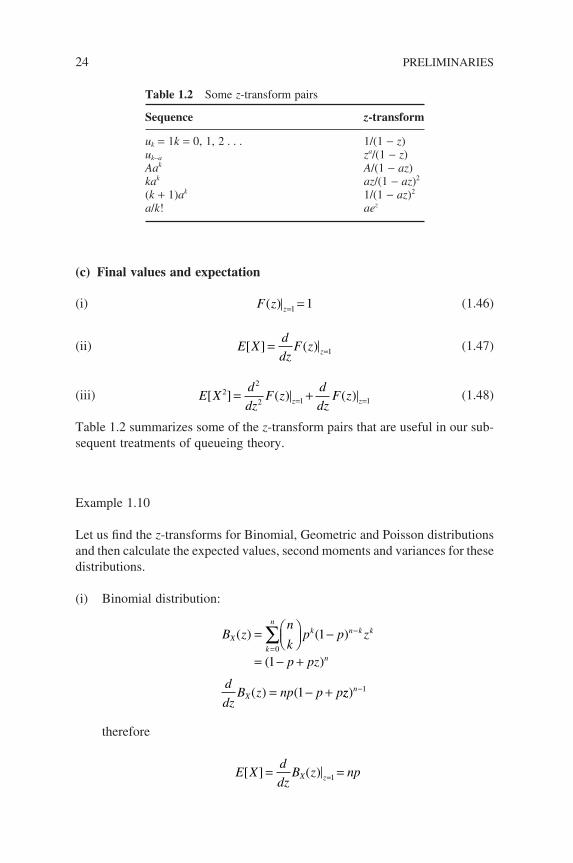
Table 1.2 summarizes some of the z-transform pairs that are useful in our sub-sequent treatments of queueing theory.
Example 1.10
Let us fi nd the z-transforms for Binomial, Geometric and Poisson distributions and then calculate the expected values, second moments and variances for these distributions.
(i) Binomial distribution:
B zn
kp p z
p pz
d
dzB z np p p
Xk
nk n k k
n
X
( ) ( )
( )
( ) (
=
−
= − +
= − +
=
−∑0
1
1
1 zz n) −1
therefore
E Xd
dzB z npX z[ ] ( )= ==1
Table 1.2 Some z-transform pairs
Sequence z-transform
uk = 1k = 0, 1, 2 . . . 1/(1 − z)uk−a za/(1 − z)Aak A/(1 − az)kak az/(1 − az)2
(k + 1)ak 1/(1 − az)2
a/k! aez
andd
dzB z np n p p pz
E X n n p np
E X E
Xn
2
22
2 2
2 2 2
1 1
1
( ) ( ) ( )
[ ] ( )
[ ]
= − − +
= − +
= −
−
σ [[ ]( )
Xnp p= −1
(ii) Geometric distribution:
G z p p zpz
p z
E Xp
p z
pz p
k
k k( ) ( )( )
[ ]( )
( )
( (
= − =− −
=− −
+−
−
=
∞−∑
1
111 1
1 1
1
1 11
1
21 1
1 1
21
2
21
2
22
−=
= −
= −
=
=
p z p
d
dzG z
p p
p p
z
z
) )
( )
σ
(iii) Poisson distribution:
G zt
ke z e e e
E Xd
dzG z
k
kt k t tz t z
z
( )( )
!
[ ] ( )
( )= = =
=
=
∞− − + − −
=
∑0
1
1
λ λ λ λ λ
== =
=
= − =
− −
=
λ λ
λ
σ λ
λte t
d
dzG z t
E X E X t
t z
z
( )
( ) ( )
[ ] [ ]
1
2
21
2
2 2 2
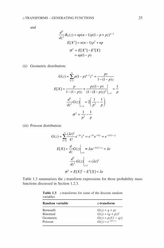
Table 1.3 summarizes the z-transform expressions for those probability mass functions discussed in Section 1.2.3.
z-TRANSFORMS – GENERATING FUNCTIONS 25
Table 1.3 z-transforms for some of the discrete random variables
Random variable z-transform
Bernoulli G(z) = q + pzBinomial G(z) = (q + pz)n
Geometric G(z) = pz/(1 − qz)Poisson G(z) = e−lt(1−z)
26 PRELIMINARIES
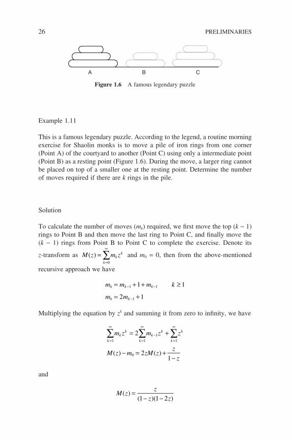
Example 1.11
This is a famous legendary puzzle. According to the legend, a routine morning exercise for Shaolin monks is to move a pile of iron rings from one corner (Point A) of the courtyard to another (Point C) using only a intermediate point (Point B) as a resting point (Figure 1.6). During the move, a larger ring cannot be placed on top of a smaller one at the resting point. Determine the number of moves required if there are k rings in the pile.
Solution
To calculate the number of moves (mk) required, we fi rst move the top (k − 1) rings to Point B and then move the last ring to Point C, and fi nally move the (k − 1) rings from Point B to Point C to complete the exercise. Denote its
z-transform as M z m zk
kk( ) =
=
∞
∑0
and m0 = 0, then from the above-mentioned
recursive approach we have
m m m k
m m
k k k
k k
= + + ≥
= +
− −
−
1 1
1
1 1
2 1
Multiplying the equation by zk and summing it from zero to infi nity, we have
kk
k
kk
k
k
km z m z z
M z m zM zz
z
=
∞
=
∞
−=
∞
∑ ∑ ∑= +
− = +−
1 11
1
0
2
21
( ) ( )
and
M zz
z z( )
( )( )=
− −1 1 2
A B C
Figure 1.6 A famous legendary puzzle
To fi nd the inverse of this expression, we do a partial fraction expansion:
M zz z
z z z( ) ( ) ( ) ( )=−
+−−
= − + − + − +1
1 2
1
12 1 2 1 2 12 2 3 3 . . .
Therefore, we have mk = 2k − 1
Example 1.12
Another well-known puzzle is the Fibonacci numbers 1, 1, 2, 3, 5, 8, 13, 21, . . ., which occur frequently in studies of population grow. This sequence of numbers is defi ned by the following recursive equation, with the initial two numbers as f0 = f1 = 1:
fk = fk−1 + fk−2 k ≥ 2
Find an explicit expression for fk.
Solution
First multiply the above equations by zk and sum it to infi nity, so we have
kk
k
kk
k
kk
kf z f z f z
F z f z f z F z f z
=
∞
=
∞
−=
∞
−∑ ∑ ∑= +
− − = − +
2 21
22
1 0 02( ) ( ( ) ) FF z
F zz z
( )
( ) =−+ −
1
12
Again, by doing a partial fraction expression, we have
F zz z z z z z
z
z
z z
( )[ ( / )] [ ( / )]
=−
−−
= + +
−
1
5 1
1
5 1
1
51
1
51
1 1 2 2
1 1 2
. . . ++ +
z
z2
. . .
where
z z1 21 5
2
1 5
2=
− +=
− −and
z-TRANSFORMS – GENERATING FUNCTIONS 27
28 PRELIMINARIES
Therefore, picking up the k term, we have
fk
k k
= +
− −
+ +1
5
1 5
2
1 5
2
1 1
1.3 LAPLACE TRANSFORMS
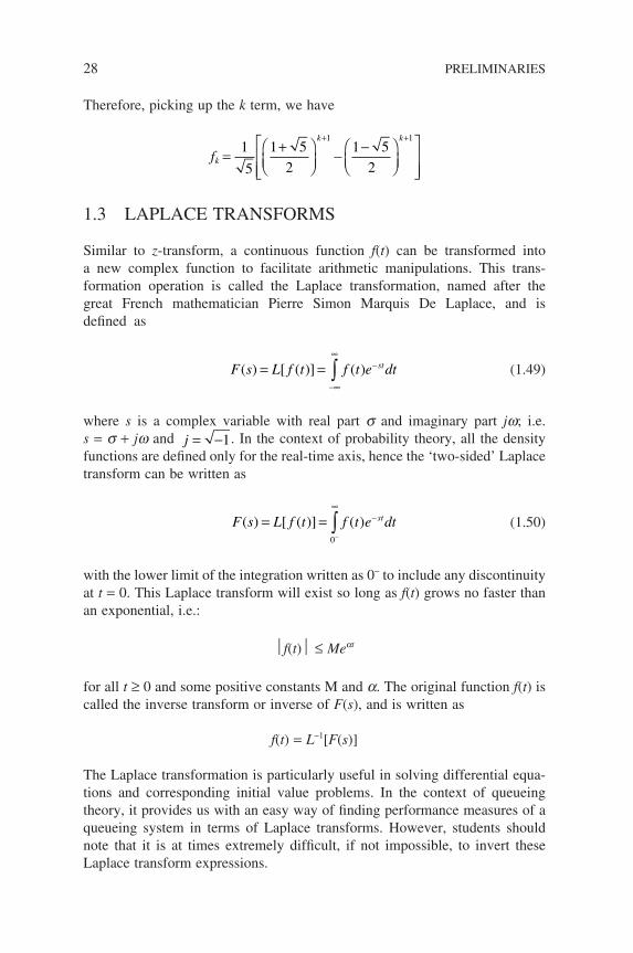
Similar to z-transform, a continuous function f(t) can be transformed into a new complex function to facilitate arithmetic manipulations. This trans-formation operation is called the Laplace transformation, named after the great French mathematician Pierre Simon Marquis De Laplace, and is defi ned as
F s L f t f t e dtst( ) [ ( )] ( )= =−∞
∞−∫ (1.49)
where s is a complex variable with real part s and imaginary part jw; i.e. s = s + jw and j = −1. In the context of probability theory, all the density functions are defi ned only for the real-time axis, hence the ‘two-sided’ Laplace transform can be written as
F s L f t f t e dtst( ) [ ( )] ( )= =−
∞−∫
0
(1.50)
with the lower limit of the integration written as 0− to include any discontinuity at t = 0. This Laplace transform will exist so long as f(t) grows no faster than an exponential, i.e.:
f(t) ≤ Meat
for all t ≥ 0 and some positive constants M and a. The original function f(t) is called the inverse transform or inverse of F(s), and is written as
f(t) = L−1[F(s)]
The Laplace transformation is particularly useful in solving differential equa-tions and corresponding initial value problems. In the context of queueing theory, it provides us with an easy way of fi nding performance measures of a queueing system in terms of Laplace transforms. However, students should note that it is at times extremely diffi cult, if not impossible, to invert these Laplace transform expressions.
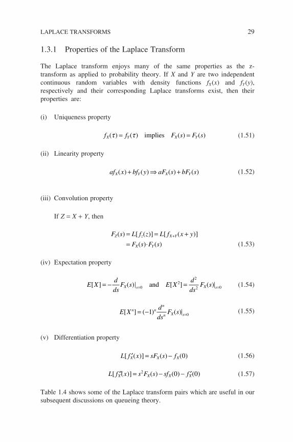
1.3.1 Properties of the Laplace Transform
The Laplace transform enjoys many of the same properties as the z-transform as applied to probability theory. If X and Y are two independent continuous random variables with density functions fX (x) and fY (y), respectively and their corresponding Laplace transforms exist, then their properties are:
(i) Uniqueness property
f f F s F sX Y X Y( ) ( ) ( ) ( )τ τ= =implies (1.51)
(ii) Linearity property
af x bf y aF s bF sX Y X Y( ) ( ) ( ) ( )+ ⇒ + (1.52)
(iii) Convolution property
If Z = X + Y, then
F s L f z L f x y
F s F sZ z X Y
X Y
( ) [ ( )] [ ( )]
( ) ( )
= = += ⋅
+ (1.53)
(iv) Expectation property
E Xd
dsF s E X
d
dsF sX s X s[ ] ( ) [ ] ( )= − == =0
22
2 0and (1.54)
E Xd
dsF sn n
n
n X s[ ] ( ) ( )= − =1 0 (1.55)
(v) Differentiation property
L f x sF s fX X X[ ( )] ( ) ( )′ = − 0 (1.56)
L f x s F s sf fX X X X[ ( )] ( ) ( ) ( )′′ = − − ′2 0 0 (1.57)
Table 1.4 shows some of the Laplace transform pairs which are useful in our subsequent discussions on queueing theory.
LAPLACE TRANSFORMS 29
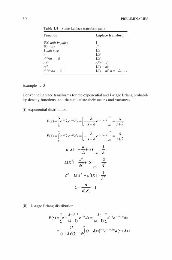
30 PRELIMINARIES
Example 1.13
Derive the Laplace transforms for the exponential and k-stage Erlang probabil-ity density functions, and then calculate their means and variances.
(i) exponential distribution
F s e e dxs
es
ss x s x( ) ( )= = −+
=+
∞− − − +
∞
∫0 0
λ λλ
λλ
λ λ
F s e e dxs
es
E Xd
dsF s
sx x s x( )
[ ] (
( )= = −+
=+
= −
∞− − − +
∞
∫0 0
λ λλ
λλ
λ λ
))
[ ] ( )
[ ] [ ]
[ ]
s
s
E Xd
dsF S
E X E X
CE X
=
=
=
= =
= − =
= =
0
22
20
2
2 2 22
1
2
1
1
λ
λ
σλ
σ
(ii) k-stage Erlang distribution
F s ex
ke dx
kx e dxss
k kx
kk s x( )
( )! ( )!( )=
−=
−
=
∞−
−−
∞− − +∫ ∫
0
1
0
1
1 1
λ λ
λ
λ λ
kk
kk s x
s ks x e d s x
( ) ( )!( ) ( )( )
+ −+ +
∞− − +∫λ
λ λλ
1 0
1
Table 1.4 Some Laplace transform pairs
Function Laplace transform
d (t) unit impulse 1d(t − a) e−as
1 unit step 1/st 1/s2
tn−1/(n − 1)! 1/sn
Aeat A/(s − a)teat 1/(s − a)2
tn−1eat/(n − 1)! 1/(s − a)n n = 1,2, . . .
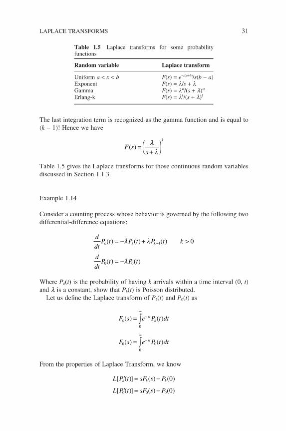
The last integration term is recognized as the gamma function and is equal to (k − 1)! Hence we have
F ss
k
( ) =+
)λ
λ
Table 1.5 gives the Laplace transforms for those continuous random variables discussed in Section 1.1.3.
Example 1.14
Consider a counting process whose behavior is governed by the following two differential-difference equations:
d
dtP t P t P t k
d
dtP t P t
k k k( ) ( ) ( )
( ) ( )
= − + >
= −
−λ λ
λ
1
0 0
0
Where Pk(t) is the probability of having k arrivals within a time interval (0, t) and l is a constant, show that Pk(t) is Poisson distributed.
Let us defi ne the Laplace transform of Pk(t) and P0(t) as
F s e P t dt
F s e P t dt
kst
k
st
( ) ( )
( ) ( )
=
=
∞−
∞−
∫
∫
0
0
0
0
From the properties of Laplace Transform, we know
L P t sF s P
L P t sF s P
k k k[ ( )] ( ) ( )
[ ( )] ( ) ( )
′ = −
′ = −
0
00 0 0
LAPLACE TRANSFORMS 31
Table 1.5 Laplace transforms for some probability functions
Random variable Laplace transform
Uniform a < x < b F(s) = e−s(a+b)/s(b − a)Exponent F(s) = l/s + lGamma F(s) = la/(s + l)a
Erlang-k F(s) = lk/(s + l)k
32 PRELIMINARIES
Substituting them into the differential-difference equations, we obtain
F sP
s
F sP L s
sk
k k
00
1
0
0
( )( )
( )( ) ( )
=+
=+
+−
λλ
λ
If we assume that the arrival process begins at time t = 0, then P0(0) = 1 and Pk(0) = 0, and we have
F ss
F ss
F ss
F s
s
k k
k
k
k
0
1 0
1
1( )
( ) ( ) ( )
( )
=+
=+
=+
)
=+
−
+
λλ
λλ
λλλ
Inverting the two transforms, we obtain the probability mass functions:
P e
P tt
ke
t
k
kt
0 0( )
( )( )
!
=
=
−
−
λ
λλ
1.4 MATRIX OPERATIONS
In Chapter 8, with the introduction of Markov-modulated arrival models, we will be moving away from the familiar Laplace (z-transform) solutions to a new approach of solving queueing systems, called matrix-geometric solutions. This particular approach to solving queueing systems was pioneered by Marcel F Neuts. It takes advantage of the similar structure presented in many interest-ing stochastic models and formulates their solutions in terms of the solution of a nonlinear matrix equation.
1.4.1 Matrix Basics
A matrix is a m × n rectangular array of real (or complex) numbers enclosed in parentheses, as shown below:
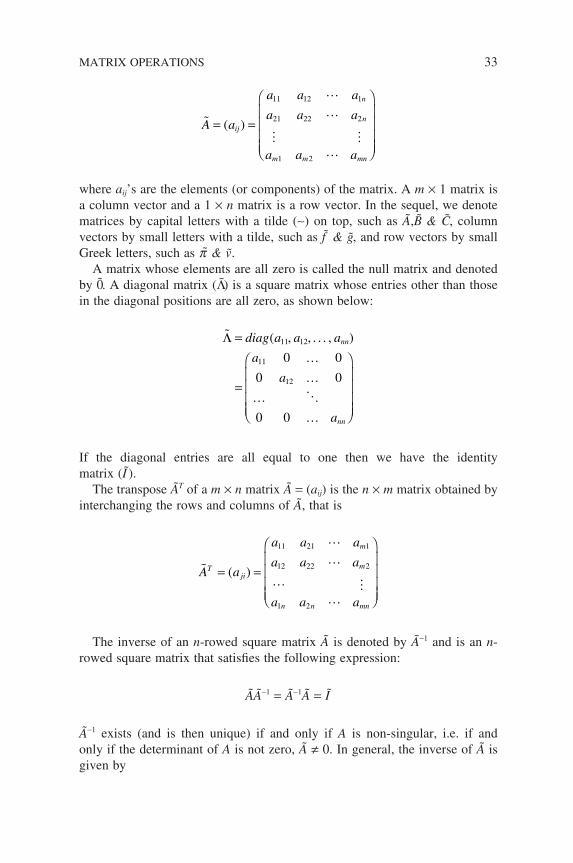
A a
a a a
a a a
a a a
ij
n
n
m m mn
= =
( )
11 12 1
21 22 2
1 2
where aij’s are the elements (or components) of the matrix. A m × 1 matrix is a column vector and a 1 × n matrix is a row vector. In the sequel, we denote matrices by capital letters with a tilde (∼) on top, such as Ã,B & C, column vectors by small letters with a tilde, such as f & g, and row vectors by small Greek letters, such as p & v.
A matrix whose elements are all zero is called the null matrix and denoted by 0. A diagonal matrix (Λ) is a square matrix whose entries other than those in the diagonal positions are all zero, as shown below:
……
… …
Λ =
=
diag a a a
a
a
a
nn
nn
( )11 12
11
12
0 0
0 0
0 0
, , . . . ,
If the diagonal entries are all equal to one then we have the identity matrix (I ).
The transpose ÃT of a m × n matrix à = (aij) is the n × m matrix obtained by interchanging the rows and columns of Ã, that is
A a
a a a
a a a
a a a
Tji
m
m
n n mn
= =
( )
11 21 1
12 22 2
1 2
The inverse of an n-rowed square matrix à is denoted by Ã−1 and is an n-rowed square matrix that satisfi es the following expression:
ÃÃ−1 = Ã−1Ã = I
Ã−1 exists (and is then unique) if and only if A is non-singular, i.e. if and only if the determinant of A is not zero, à ≠ 0. In general, the inverse of à is given by
MATRIX OPERATIONS 33
34 PRELIMINARIES
…
… …A
A
A A A
A A
A A A
n
n n nn
− =
1
11 21 1
12 22
1 2
1
det
where Aij is the cofactor of aij in Ã. The cofactor of aij is the product of (−1)i+j and the determinant formed by deleting the ith row and the jth column from the det Ã. For a 2 × 2 matrix Ã, the inverse is given by
Aa a
a aA
a a a a
a a
a a=
=
−−
−−11 12
21 22
1
11 22 21 12
22 12
21 11
1and
We summarize some of the properties of matrixes that are useful in manipu-lating them. In the following expressions, a and b are numbers:
(i) a(à + B) = aà + aB and (a + b)à = aà + bÃ(ii) (aÃ)B = a(ÃB) = Ã(aB) and Ã(BC) = (ÃB)C(iii) (à + B)C = ÃC + BC and C(à + B) = Cà + CB(iv) ÃB ≠ Bà in general(v) ÃB = 0 does not necessarily imply à = 0 or B = 0(vi) (à + B)T = ÃT + BT and (ÃT)T = Ã(vii) (ÃB)T = BTÃT and det à = det ÃT
(viii) (Ã−1)−1 = Ã and (ÃB)−1 = B−1Ã−1
(ix) (Ã−1)T = (ÃT)−1 and (Ã2)−1 = (Ã−1)2
1.4.2 Eigenvalues, Eigenvectors and Spectral Representation
An eigenvalue (or characteristic value) of an n × n square matrix à = (aij) is a real or complex scalar l satisfying the following vector equation for some non-zero (column) vector x of dimension n × 1. The vector x is known as the eigenvector, or more specifi cally the column (or right) eigenvector:
Ax x= λ (1.58)
This equation can be rewritten as (Ã − lI )x = 0 and has a non-zero solution x only if (Ã − lI ) is singular; that is to say that any eigenvalue must satisfy det(Ã − lI ) = 0. This equation, det(Ã − lI ) = 0, is a polynomial of degree n in l and has exactly n real or complex roots, including multiplicity. Therefore,
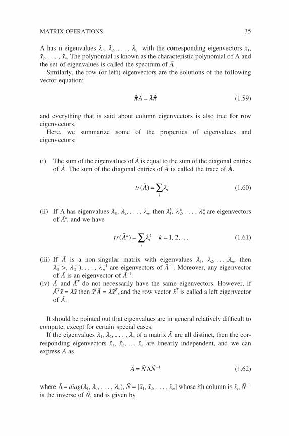
A has n eigenvalues l1, l2, . . . , ln with the corresponding eigenvectors x1, x2, . . . , xn. The polynomial is known as the characteristic polynomial of A and the set of eigenvalues is called the spectrum of Ã.
Similarly, the row (or left) eigenvectors are the solutions of the following vector equation:
π λπA = (1.59)
and everything that is said about column eigenvectors is also true for row eigenvectors.
Here, we summarize some of the properties of eigenvalues and eigenvectors:
(i) The sum of the eigenvalues of à is equal to the sum of the diagonal entries of Ã. The sum of the diagonal entries of à is called the trace of Ã.
tr Ai
i( ) = ∑λ (1.60)
(ii) If A has eigenvalues l1, l2, . . . , ln, then lk1, l k2, . . . , l kn are eigenvectors
of Ãk, and we have
tr A kk
iik( ) = =∑λ 1 2, , . . . (1.61)
(iii) If à is a non-singular matrix with eigenvalues l1, l2, . . . ,ln, then l1
−1>, l 2−1), . . . , l n−1 are eigenvectors of Ã−1. Moreover, any eigenvector of à is an eigenvector of Ã−1.
(iv) Ã and ÃT do not necessarily have the same eigenvectors. However, if ÃTx = lx then xTÃ = lxT, and the row vector xT is called a left eigenvector of Ã.
It should be pointed out that eigenvalues are in general relatively diffi cult to compute, except for certain special cases.
If the eigenvalues l1, l2, . . . , ln of a matrix à are all distinct, then the cor-responding eigenvectors x1, x2, ..., xn are linearly independent, and we can express à as
A N N= −Λ 1 (1.62)
where Λ = diag(l1, l2, . . . , ln), Ñ = [x1, x2, . . . , xn] whose ith column is xi, Ñ −1 is the inverse of Ñ, and is given by
MATRIX OPERATIONS 35
36 PRELIMINARIES
…
N
n
− =
1
1
2
ππ
π
By induction, it can be shown that Ãk = ÑΛkÑ−1.If we defi ne Bk to be the matrix obtained by multiplying the column vector
xk with the row vector pk, then we have
…… …
…
B x
x x n
x n x n n
k k k
k k k k
k k k k
=
=
ππ π
π π
( ) ( ) ( ) ( )
( ) ( ) ( ) ( )
1 1 1
1
(1.63)
It can be shown that
A N N
B B Bn n
=
= + + +
−Λ 1
1 1 2 2λ λ λ. . .
(1.64)
and
A B B Bk k knk
n= + + +λ λ λ11 1 2 2 . . . (1.65)
The expression of à in terms of its eigenvalues and the matrices Bk is called the spectral representation of Ã.
1.4.3 Matrix Calculus
Let us consider the following set of ordinary differential equations with con-stant coeffi cients and given initial conditions:
d
dtx t a x t a x t a x t
d
dtx t a x t
n n
n n
1 11 1 11 2 1
1 1
( ) ( ) ( ) ( )
( ) ( )
= + + +
= +
. . .
aa x t a x tn nn n2 2( ) ( )+ +. . .
(1.66)
In matrix notation, we have
x t Ax t( ) ( )′ = (1.67)
where x(t) is a n × 1 vector whose components xi(t)are functions of an inde-pendent variable t, and x(t)′ denotes the vector whose components are the derivatives dxi /dt. There are two ways of solving this vector equation:
(i) First let us assume that x(t) = eltp, where P is a scalar vector and substitute it in Equation (1.67), then we have
leltp = Ã(eltp)
Since elt ≠ 0, it follows that l and p must satisfy Ãp = l p; therefore, if li is an eigenvector of A and pi is a corresponding eigenvector, then elitpi is a solution. The general solution is given by
x t e pi
n
it
ii( ) =
=∑
1
α λ (1.68)
where ai is the constant chosen to satisfy the initial condition of Equation (1.67).
(ii) The second method is to defi ne the matrix exponential eÃt through the convergent power series as
exp . . . +(
( )
!
( )
!
)
!
At
At
kI At
At At
kk
k k
= = + + +=
∞
∑0
2
2 (1.69)
By differentiating the expression with respect to t directly, we have
d
dte A A t
A t
A I AtA t
At( )!
!
= + + +
= + + +
=
23 2
2 2
2
2
. . .
. . . AAeAt
Therefore, eÃt is a solution to Equation (1.67) and is called the fundamental matrix for (1.67).
We summarize some of the useful properties of the matrix exponential below:
MATRIX OPERATIONS 37
38 PRELIMINARIES
(i) eÃ(s+t) = eÃseÃt
(ii) eÃt is never singular and its inverse is e−Ãt
(iii) e(Ã+B)t = eÃteBt for all t, only if ÃB = BÃ
(iv) d
dte Ae e AAt At At = =
(v) ( ) I A A I A Ai
i− = = + + +−
=
∞
∑1
0
2 . . .
(vi) eÃt = ÑeΛ tÑ−1 = el1tB1 + el2tB2 + . . . + elntBn
where
e
e
e
t
t
tn
Λ =
λ
λ
1 0
0
and Bi are as defi ned in Equation (1.63).Now let us consider matrix functions. The following are examples:
A tt
t tA( ) ( )=
=
−
0
42and
sin cos
0 sinθ
θ θθ
We can easily extend the calculus of scalar functions to matrix functions. In the following, Ã(t) and B(t) are matrix functions with independent variable t and U a matrix of real constants:
(i) d
dtU = 0
(ii) d
dtA t B t
d
dtA t
d
dtB t( ( ) ( )) ( ) ( )α β α β + = +
(iii) d
dtA t B t
d
dtA t B t A t
d
dtB t( ( ) ( )) ( ) ( ) ( ) ( ) =
) + )
(iv) d
dtA t
d
dtA t A t A t
d
dtA t 2( ) ( ) ( ) ( ) ( )=
) + )
(v) d
dtA t A t
d
dtA t A t − − −= −
)1 1 1( ) ( ) ( ) ( )
(vi) d
dtA t
d
dtA tT
T
( ( )) ( ) = )
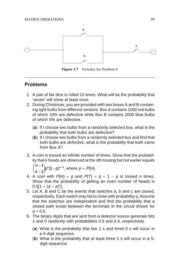
Problems
1. A pair of fair dice is rolled 10 times. What will be the probability that ‘seven’ will show at least once.
2. During Christmas, you are provided with two boxes A and B contain-ing light bulbs from different vendors. Box A contains 1000 red bulbs of which 10% are defective while Box B contains 2000 blue bulbs of which 5% are defective.
(a) If I choose two bulbs from a randomly selected box, what is the probability that both bulbs are defective?
(b) If I choose two bulbs from a randomly selected box and fi nd that both bulbs are defective, what is the probability that both came from Box A?
3. A coin is tossed an infi nite number of times. Show that the probabil-ity that k heads are observed at the nth tossing but not earlier equals
n
kn−
−
− −1
11p p)k k( , where p = PH.
4. A coin with PH = p and PT = q = 1 − p is tossed n times. Show that the probability of getting an even number of heads is 0.5[1 + (q − p)n].
5. Let A, B and C be the events that switches a, b and c are closed, respectively. Each switch may fail to close with probability q. Assume that the switches are independent and fi nd the probability that a closed path exists between the terminals in the circuit shown for q = 0.5.
6. The binary digits that are sent from a detector source generate bits 1 and 0 randomly with probabilities 0.6 and 0.4, respectively.
(a) What is the probability that two 1 s and three 0 s will occur in a 5-digit sequence.
(b) What is the probability that at least three 1 s will occur in a 5-digit sequence.
MATRIX OPERATIONS 39
a
b
c
Figure 1.7 Switches for Problem 6
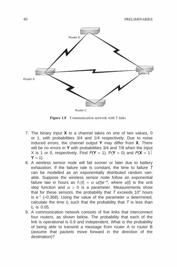
40 PRELIMINARIES
7. The binary input X to a channel takes on one of two values, 0 or 1, with probabilities 3/4 and 1/4 respectively. Due to noise induced errors, the channel output Y may differ from X. There will be no errors in Y with probabilities 3/4 and 7/8 when the input X is 1 or 0, respectively. Find P(Y = 1), P(Y = 0) and P(X = 1Y = 1).
8. A wireless sensor node will fail sooner or later due to battery exhaustion. If the failure rate is constant, the time to failure T can be modelled as an exponentially distributed random vari-able. Suppose the wireless sensor node follow an exponential failure law in hours as fT (t) = a u(t)e−at, where u(t) is the unit step function and a > 0 is a parameter. Measurements show that for these sensors, the probability that T exceeds 104 hours is e−1 (≈0.368). Using the value of the parameter a determined, calculate the time t0 such that the probability that T is less than t0 is 0.05.
9. A communication network consists of fi ve links that interconnect four routers, as shown below. The probability that each of the link is operational is 0.9 and independent. What is the probability of being able to transmit a message from router A to router B (assume that packets move forward in the direction of the destination)?
Router B
Router A
Router D
Router C
Figure 1.8 Communication network with 5 links
10. Two random variables X and Y take on the values i and 2i with probability 1/2i (i = 1,2, . . .). Show that the probabilities sum to one. Find the expected value of X and Y.
11. There are three identical cards, one is red on both sides, one is yellow on both sides and the last one is red on one side and yellow on the other side. A card is selected at random and is red on the upper side. What is the probability that the other side is yellow?
MATRIX OPERATIONS 41

2Introduction to Queueing Systems
In today’s information age society, where activities are highly interdependent and intertwined, sharing of resources and hence waiting in queues is a common phenomenon that occurs in every facet of our lives. In the context of data com-munication, expensive transmission resources in public data networks, such as the Internet, are shared by various network users. Data packets are queued in the buffers of switching nodes while waiting for transmission. In a computer system, computer jobs are queued for CPU or I/O devices in various stages of their processing.
The understanding and prediction of the stochastic behaviour of these queues will provide a theoretical insight into the dynamics of these shared resources and how they can be designed to provide better utilization. The modelling and analysis of waiting queues/networks and their applications in data communica-tions is the main subject of this book. The study of queues comes under a discipline of Operations Research called Queueing Theory and is a pri-mary methodological framework for evaluating resource performance besides simulation.
The origin of queueing theory can be traced back to early in the last century when A K Erlang, a Danish engineer, applied this theory extensively to study the behaviour of telephone networks. Acknowledged to be the father of queue-ing theory, Erlang developed several queueing results that still remain the backbone of queueing performance evaluations today.
In this chapter, you will be introduced to the basic structure, the terminology and the characteristics before embarking on the actual study of queueing
Queueing Modelling Fundamentals Second Edition Ng Chee-Hock and Soong Boon-Hee© 2008 John Wiley & Sons, Ltd
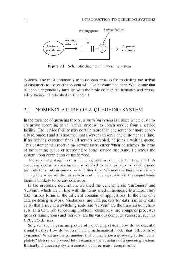
44 INTRODUCTION TO QUEUEING SYSTEMS
systems. The most commonly used Poisson process for modelling the arrival of customers to a queueing system will also be examined here. We assume that students are generally familiar with the basic college mathematics and proba-bility theory, as refreshed in Chapter 1.
2.1 NOMENCLATURE OF A QUEUEING SYSTEM
In the parlance of queueing theory, a queueing system is a place where custom-ers arrive according to an ‘arrival process’ to obtain service from a service facility. The service facility may contain more than one server (or more gener-ally resources) and it is assumed that a server can serve one customer at a time. If an arriving customer fi nds all servers occupied, he joins a waiting queue. This customer will receive his service later, either when he reaches the head of the waiting queue or according to some service discipline. He leaves the system upon completion of his service.
The schematic diagram of a queueing system is depicted in Figure 2.1. A queueing system is sometimes just referred to as a queue, or queueing node (or node for short) in some queueing literature. We may use these terms inter-changeably when we discuss networks of queueing systems in the sequel when there is unlikely to be any confusion.
In the preceding description, we used the generic terms ‘customers’ and ‘servers’, which are in line with the terms used in queueing literature. They take various forms in the different domains of applications. In the case of a data switching network, ‘customers’ are data packets (or data frames or data cells) that arrive at a switching node and ‘servers’ are the transmission chan-nels. In a CPU job scheduling problem, ‘customers’ are computer processes (jobs or transactions) and ‘servers’ are the various computer resources, such as CPU, I/O devices.
So given such a dynamic picture of a queueing system, how do we describe it analytically? How do we formulate a mathematical model that refl ects these dynamics? What are the parameters that characterize a queueing system com-pletely? Before we proceed let us examine the structure of a queueing system. Basically, a queueing system consists of three major components:
Customerpopulation
Departingcustomers
Arrivingcustomers
Waiting queue Service facility
Figure 2.1 Schematic diagram of a queneing system
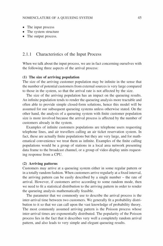
NOMENCLATURE OF A QUEUEING SYSTEM 45
• The input process
• The system structure
• The output process.
2.1.1 Characteristics of the Input Process
When we talk about the input process, we are in fact concerning ourselves with the following three aspects of the arrival process:
(1) The size of arriving populationThe size of the arriving customer population may be infi nite in the sense that the number of potential customers from external sources is very large compared to those in the system, so that the arrival rate is not affected by the size.
The size of the arriving population has an impact on the queueing results. An infi nite population tends to render the queueing analysis more tractable and often able to provide simple closed-form solutions, hence this model will be assumed for our subsequent queueing systems unless otherwise stated. On the other hand, the analysis of a queueing system with fi nite customer population size is more involved because the arrival process is affected by the number of customers already in the system.
Examples of infi nite customers populations are telephone users requesting telephone lines, and air travellers calling an air ticket reservation system. In fact, these are actually fi nite populations but they are very large, and for math-ematical convenience we treat them as infi nite. Examples of the fi nite calling populations would be a group of stations in a local area network presenting data frame to the broadcast channel, or a group of video display units request-ing response from a CPU.
(2) Arriving patternsCustomers may arrive at a queueing system either in some regular pattern or in a totally random fashion. When customers arrive regularly at a fi xed interval, the arriving pattern can be easily described by a single number – the rate of arrival. However, if customers arrive according to some random mode, then we need to fi t a statistical distribution to the arriving pattern in order to render the queueing analysis mathematically feasible.
The parameter that we commonly use to describe the arrival process is the inter-arrival time between two customers. We generally fi t a probability distri-bution to it so that we can call upon the vast knowledge of probability theory. The most commonly assumed arriving pattern is the Poisson process whose inter-arrival times are exponentially distributed. The popularity of the Poisson process lies in the fact that it describes very well a completely random arrival pattern, and also leads to very simple and elegant queueing results.
46 INTRODUCTION TO QUEUEING SYSTEMS
We list below some probability distributions that are commonly used to describe the inter-arrival time of an arrival process. These distributions are generally denoted by a single letter as shown:
M: Markovian (or Memoryless), imply Poisson processD: Deterministic, constant interarrival timesEk: Erlang distribution of order K of inter-arrival timesG: General probability distribution of inter-arrival timesGI: General and independent (inter-arrival time) distribution.
(3) Behaviour of arriving customersCustomers arriving at a queueing system may behave differently when the system is full due to a fi nite waiting queue or when all servers are busy. If an arriving customer fi nds the system is full and leaves forever without entering the system, that queueing system is referred to as a blocking system. The analysis of blocking systems, especially in the case of queueing networks, is more involved and at times it is impossible to obtain closed-form results. We will assume that this is the behaviour exhibited by all arriving customers in our subsequent queueing models. In real life, customers tend to come back after a short while.
In telephone networks, call requests that are blocked when the network is busy are said to employ a lost-calls-cleared discipline. The key measure of performance in such a system is the probability of blocking that a call experi-ences. We will discuss blocking probability in greater detail in Chapter 4. On the other hand, if calls are placed in queues, it is referred to as lost-calls-delayed. The measure of performance is the elapsed time of a call.
2.1.2 Characteristics of the System Structure
(i) Physical number and layout of serversThe service facility shown in Figure 2.1 may comprise of one or more servers. In the context of this book, we are interested only in the parallel and identical servers; that is a customer at the head of the waiting queue can go to any server that is free, and leave the system after receiving his/her service from that server, as shown in Figure 2.2 (a). We will not concern ourselves with the serial-servers case where a customer receives services from all or some of them in stages before leaving the system, as shown in Figure 2.2 (b).
(ii) The system capacityThe system capacity refers to the maximum number of customers that a queue-ing system can accommodate, inclusive of those customers at the service facility.
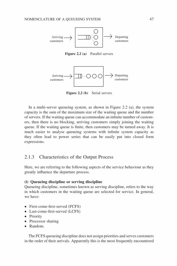
NOMENCLATURE OF A QUEUEING SYSTEM 47
In a multi-server queueing system, as shown in Figure 2.2 (a), the system capacity is the sum of the maximum size of the waiting queue and the number of servers. If the waiting queue can accommodate an infi nite number of custom-ers, then there is no blocking, arriving customers simply joining the waiting queue. If the waiting queue is fi nite, then customers may be turned away. It is much easier to analyse queueing systems with infi nite system capacity as they often lead to power series that can be easily put into closed form expressions.
2.1.3 Characteristics of the Output Process
Here, we are referring to the following aspects of the service behaviour as they greatly infl uence the departure process.
(i) Queueing discipline or serving disciplineQueueing discipline, sometimes known as serving discipline, refers to the way in which customers in the waiting queue are selected for service. In general, we have:
• First-come-fi rst-served (FCFS)
• Last-come-fi rst-served (LCFS)
• Priority
• Processor sharing
• Random.
The FCFS queueing discipline does not assign priorities and serves customers in the order of their arrivals. Apparently this is the most frequently encountered
Arrivingcustomers
Departingcustomers
Arrivingcustomers
Departingcustomers
Figure 2.2 (a) Parallel servers
Figure 2.2 (b) Serial servers
48 INTRODUCTION TO QUEUEING SYSTEMS
discipline at an ordered queue and therefore it will be the default queueing disci-pline for all the subsequent systems discussed, unless otherwise stated.
The LCFS discipline is just the reverse of FCFS. Customers who come last will be served fi rst. This type of queueing discipline is commonly found in stack operations where items (customers in our terminology) are stacked and operations occur only at the top of the stack.
In priority queueing discipline, customers are divided into several priority classes according to their assigned priorities. Those having a higher priority than others are served fi rst before others receiving their service. There are two sub-classifi cations: preemptive and non-preemptive. Their defi nitions and oper-ations will be discussed in detail in Chapter 5.
In processor sharing, capacity is equally divided among all customers in the queue, that is when there are k customers, the server devotes 1/k of his capacity to each. Equally, each customer obtains service at 1/k of rate and leaves the system upon completion of his service.
(ii) Service-time distributionSimilar to arrival patterns, if all customers require the same amount of service time then the service pattern can be easily described by a single number. But generally, different customers require different amounts of service times, hence we again use a probability distribution to describe the length of service times the server renders to those customers. The most commonly assumed service time distribution is the negative exponential distribution.
Again, we commonly use a single letter to indicate the type of service distributions:
M: Markovian (or Memoryless) , imply exponential distributed service timesD: Deterministic ; constant service timesEk: Erlang of order K service time distributionG: General service times distribution.
2.2 RANDOM VARIABLES AND THEIR RELATIONSHIPS
From the preceding description of a queueing system, we see that customers arrive, are served and leave the system, hence presenting a fl uid situation with constant motions. There are many processes present and interacting with each other. Most of the quantities associated with these processes evolve in time and are of a probabilistic nature. In other words, they are the so-called random variables and their values can only be expressed through probability. We sum-marize the primary random variables of a queueing system in Table 2.1 and list some of the relationships among them.
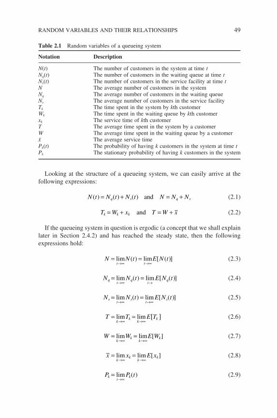
Looking at the structure of a queueing system, we can easily arrive at the following expressions:
N t N t N t N N Nq s q s( ) ( ) ( )= + = +and (2.1)
T W x T W xk k k= + = +and (2.2)
If the queueing system in question is ergodic (a concept that we shall explain later in Section 2.4.2) and has reached the steady state, then the following expressions hold:
N N t E N tt t
= =→∞ →∞
lim lim( ) [ ( )] (2.3)
N N t E N tqt
qt
q= =→∞ →
lim lim( ) [ ( )] (2.4)
N N t E N tst
st
s= =→∞ →∞
lim lim( ) [ ( )] (2.5)
T T E Tk
kk
k= = [ ]→∞ →∞
lim lim (2.6)
W W E Wk
kk
k= =→∞ →∞
lim lim [ ] (2.7)
x x E xk
kk
k= =→∞ →∞
lim lim [ ] (2.8)
P P tkt
k=→∞
lim ( ) (2.9)
Table 2.1 Random variables of a queueing system
Notation Description
N(t) The number of customers in the system at time tNq(t) The number of customers in the waiting queue at time tNs(t) The number of customers in the service facility at time tN The average number of customers in the systemNq The average number of customers in the waiting queueNs The average number of customers in the service facilityTk The time spent in the system by kth customerWk The time spent in the waiting queue by kth customerxk The service time of kth customerT The average time spent in the system by a customerW The average time spent in the waiting queue by a customerx The average service timePk(t) The probability of having k customers in the system at time tPk The stationary probability of having k customers in the system
RANDOM VARIABLES AND THEIR RELATIONSHIPS 49
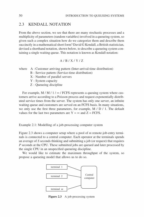
50 INTRODUCTION TO QUEUEING SYSTEMS
2.3 KENDALL NOTATION
From the above section, we see that there are many stochastic processes and a multiplicity of parameters (random variables) involved in a queueing system, so given such a complex situation how do we categorize them and describe them succinctly in a mathematical short form? David G Kendall, a British statistician, devised a shorthand notation, shown below, to describe a queueing system con-taining a single waiting queue. This notation is known as Kendall notation:
A / B / X / Y / Z
where A : Customer arriving pattern (Inter-arrival-time distribution) B : Service pattern (Service-time distribution) X : Number of parallel servers Y : System capacity Z : Queueing discipline
For example, M / M / 1 / ∞ / FCFS represents a queuing system where cus-tomers arrive according to a Poisson process and request exponentially distrib-uted service times from the server. The system has only one server, an infi nite waiting queue and customers are served on an FCFS basis. In many situations, we only use the fi rst three parameters, for example, M / D / 1. The default values for the last two parameters are Y = ∞ and Z = FCFS.
Example 2.1: Modelling of a job-processing computer system
Figure 2.3 shows a computer setup where a pool of m remote-job-entry termi-nals is connected to a central computer. Each operator at the terminals spends an average of S seconds thinking and submitting a job (or request) that requires P seconds at the CPU. These submitted jobs are queued and later processed by the single CPU in an unspecifi ed queueing discipline.
We would like to estimate the maximum throughput of the system, so propose a queueing model that allows us to do so.
Centralcomputer
terminal 1
terminal 2
terminal m
Figure 2.3 A job-processing system
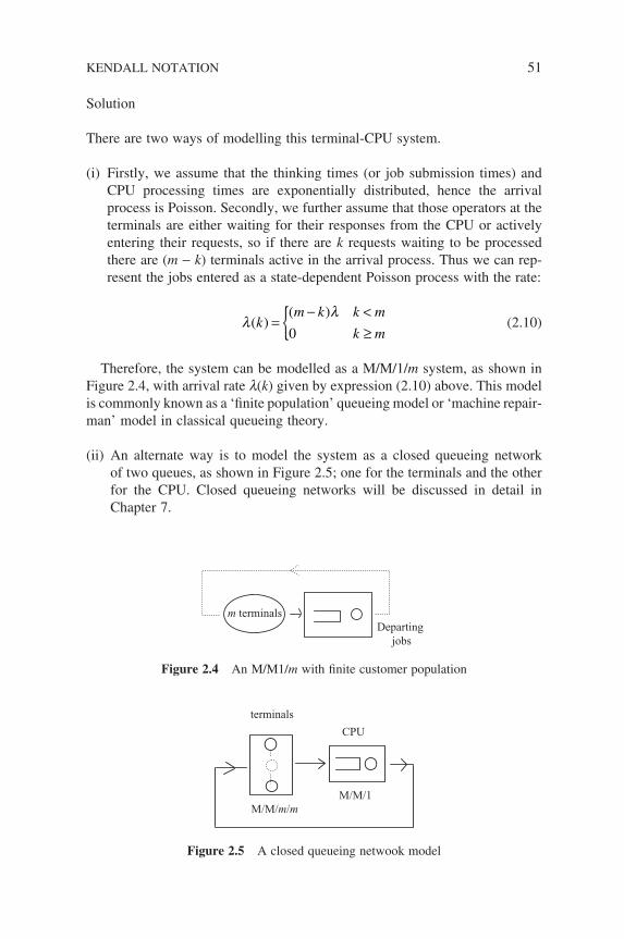
Solution
There are two ways of modelling this terminal-CPU system.
(i) Firstly, we assume that the thinking times (or job submission times) and CPU processing times are exponentially distributed, hence the arrival process is Poisson. Secondly, we further assume that those operators at the terminals are either waiting for their responses from the CPU or actively entering their requests, so if there are k requests waiting to be processed there are (m − k) terminals active in the arrival process. Thus we can rep-resent the jobs entered as a state-dependent Poisson process with the rate:
λλ
( )( )
km k k m
k m=
− <≥0
(2.10)
Therefore, the system can be modelled as a M/M/1/m system, as shown in Figure 2.4, with arrival rate l(k) given by expression (2.10) above. This model is commonly known as a ‘fi nite population’ queueing model or ‘machine repair-man’ model in classical queueing theory.
(ii) An alternate way is to model the system as a closed queueing network of two queues, as shown in Figure 2.5; one for the terminals and the other for the CPU. Closed queueing networks will be discussed in detail in Chapter 7.
m terminalsDeparting
jobs
Figure 2.4 An M/M1/m with fi nite customer population
terminals
CPU
M/M/m/mM/M/1
Figure 2.5 A closed queueing netwook model
KENDALL NOTATION 51
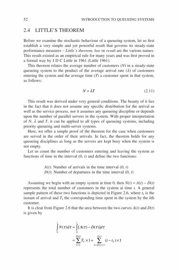
52 INTRODUCTION TO QUEUEING SYSTEMS
2.4 LITTLE’S THEOREM
Before we examine the stochastic behaviour of a queueing system, let us fi rst establish a very simple and yet powerful result that governs its steady-state performance measures – Little’s theorem, law or result are the various names. This result existed as an empirical rule for many years and was fi rst proved in a formal way by J D C Little in 1961 (Little 1961).
This theorem relates the average number of customers (N) in a steady-state queueing system to the product of the average arrival rate (l) of customers entering the system and the average time (T) a customer spent in that system, as follows:
N T= λ (2.11)
This result was derived under very general conditions. The beauty of it lies in the fact that it does not assume any specifi c distribution for the arrival as well as the service process, nor it assumes any queueing discipline or depends upon the number of parallel servers in the system. With proper interpretation of N, l and T, it can be applied to all types of queueing systems, including priority queueing and multi-server systems.
Here, we offer a simple proof of the theorem for the case when customers are served in the order of their arrivals. In fact, the theorem holds for any queueing disciplines as long as the servers are kept busy when the system is not empty.
Let us count the number of customers entering and leaving the system as functions of time in the interval (0, t) and defi ne the two functions:
A(t): Number of arrivals in the time interval (0, t)D(t): Number of departures in the time interval (0, t)
Assuming we begin with an empty system at time 0, then N(t) = A(t) − D(t) represents the total number of customers in the system at time t. A general sample pattern of these two functions is depicted in Figure 2.6, where tk is the instant of arrival and Tk the corresponding time spent in the system by the kth customer.
It is clear from Figure 2.6 that the area between the two curves A(t) and D(t) is given by
N d A D d
T t t
tt
k kk D t
A t
k
D
( ) [ ( ) ( )]
( )( )
( )(
τ τ τ τ τ= −
= × + − ×
∫∫
∑= +=
00
11
1 1tt )
∑
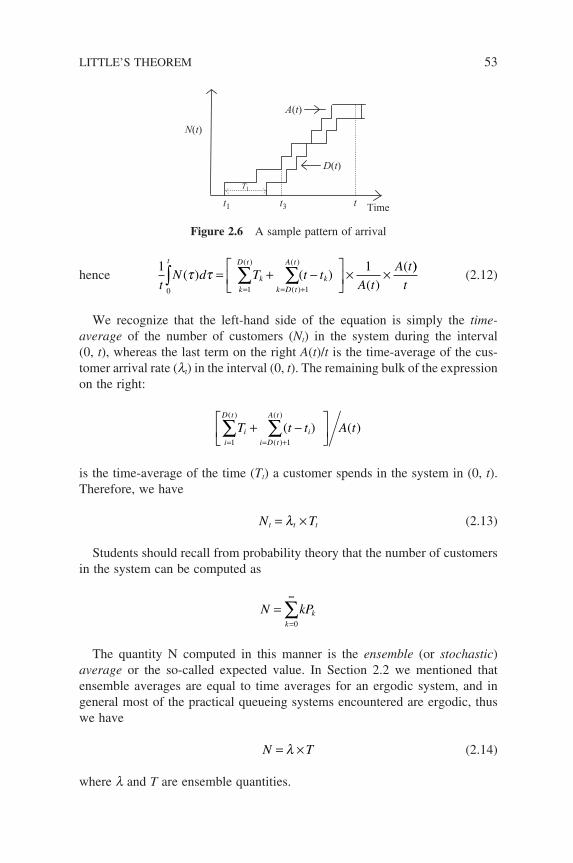
hence 1 1
0 1 1tN d T t t
A t
A tt
k
D t
kk D t
A t
k∫ ∑ ∑= + −
× ×
= = +
( ) ( )( )
(( )
( )
( )
τ τ ))
t (2.12)
We recognize that the left-hand side of the equation is simply the time-average of the number of customers (Nt) in the system during the interval (0, t), whereas the last term on the right A(t)/t is the time-average of the cus-tomer arrival rate (lt) in the interval (0, t). The remaining bulk of the expression on the right:
i
D t
ii D t
A t
iT t t A t= = +∑ ∑+ −
1 1
( )
( )
( )
( ) ( )
is the time-average of the time (Tt) a customer spends in the system in (0, t). Therefore, we have
N Tt t t= ×λ (2.13)
Students should recall from probability theory that the number of customers in the system can be computed as
N kPk
k==
∞
∑0
The quantity N computed in this manner is the ensemble (or stochastic) average or the so-called expected value. In Section 2.2 we mentioned that ensemble averages are equal to time averages for an ergodic system, and in general most of the practical queueing systems encountered are ergodic, thus we have
N T= ×λ (2.14)
where l and T are ensemble quantities.
N(t)
Time
T1
t1 t3 t
A(t)
D(t)
Figure 2.6 A sample pattern of arrival
LITTLE’S THEOREM 53
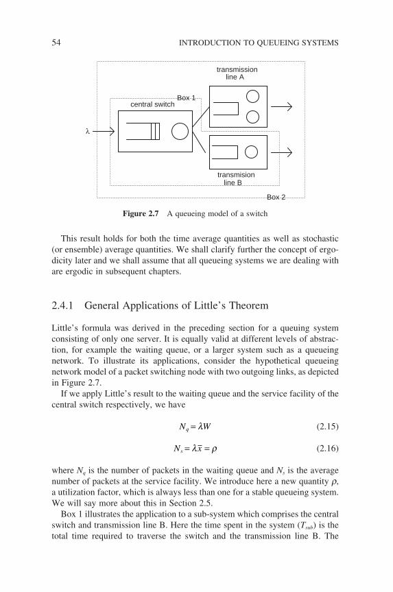
54 INTRODUCTION TO QUEUEING SYSTEMS
This result holds for both the time average quantities as well as stochastic (or ensemble) average quantities. We shall clarify further the concept of ergo-dicity later and we shall assume that all queueing systems we are dealing with are ergodic in subsequent chapters.
2.4.1 General Applications of Little’s Theorem
Little’s formula was derived in the preceding section for a queuing system consisting of only one server. It is equally valid at different levels of abstrac-tion, for example the waiting queue, or a larger system such as a queueing network. To illustrate its applications, consider the hypothetical queueing network model of a packet switching node with two outgoing links, as depicted in Figure 2.7.
If we apply Little’s result to the waiting queue and the service facility of the central switch respectively, we have
N Wq = λ (2.15)
N xs = =λ ρ (2.16)
where Nq is the number of packets in the waiting queue and Ns is the average number of packets at the service facility. We introduce here a new quantity r, a utilization factor, which is always less than one for a stable queueing system. We will say more about this in Section 2.5.
Box 1 illustrates the application to a sub-system which comprises the central switch and transmission line B. Here the time spent in the system (Tsub) is the total time required to traverse the switch and the transmission line B. The
central switch
transmission
transmisionline B
line A
Box 2
Box 1
λ
Figure 2.7 A queueing model of a switch
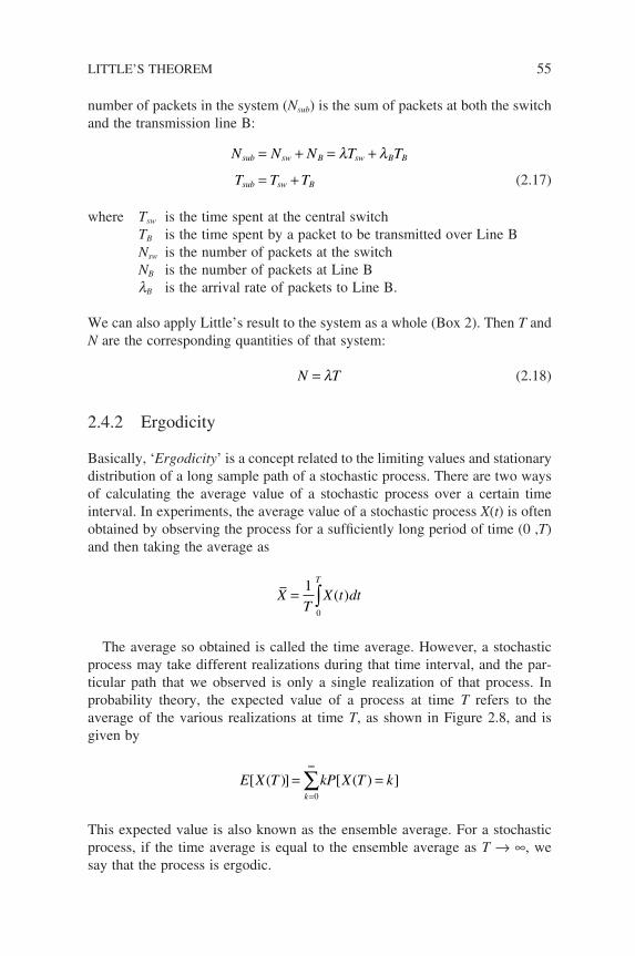
number of packets in the system (Nsub) is the sum of packets at both the switch and the transmission line B:
N N N T T
T T T
sub sw B sw B B
sub sw B
= + = +
= +
λ λ
(2.17)
where Tsw is the time spent at the central switch TB is the time spent by a packet to be transmitted over Line B Nsw is the number of packets at the switch NB is the number of packets at Line B lB is the arrival rate of packets to Line B.
We can also apply Little’s result to the system as a whole (Box 2). Then T and N are the corresponding quantities of that system:
N T= λ (2.18)
2.4.2 Ergodicity
Basically, ‘Ergodicity’ is a concept related to the limiting values and stationary distribution of a long sample path of a stochastic process. There are two ways of calculating the average value of a stochastic process over a certain time interval. In experiments, the average value of a stochastic process X(t) is often obtained by observing the process for a suffi ciently long period of time (0 ,T) and then taking the average as
XT
X t dtT
= ∫1
0
( )
The average so obtained is called the time average. However, a stochastic process may take different realizations during that time interval, and the par-ticular path that we observed is only a single realization of that process. In probability theory, the expected value of a process at time T refers to the average of the various realizations at time T, as shown in Figure 2.8, and is given by
E X T kP X T kk
[ ( )] [ ( ) ]= ==
∞
∑0
This expected value is also known as the ensemble average. For a stochastic process, if the time average is equal to the ensemble average as T → ∞, we say that the process is ergodic.
LITTLE’S THEOREM 55
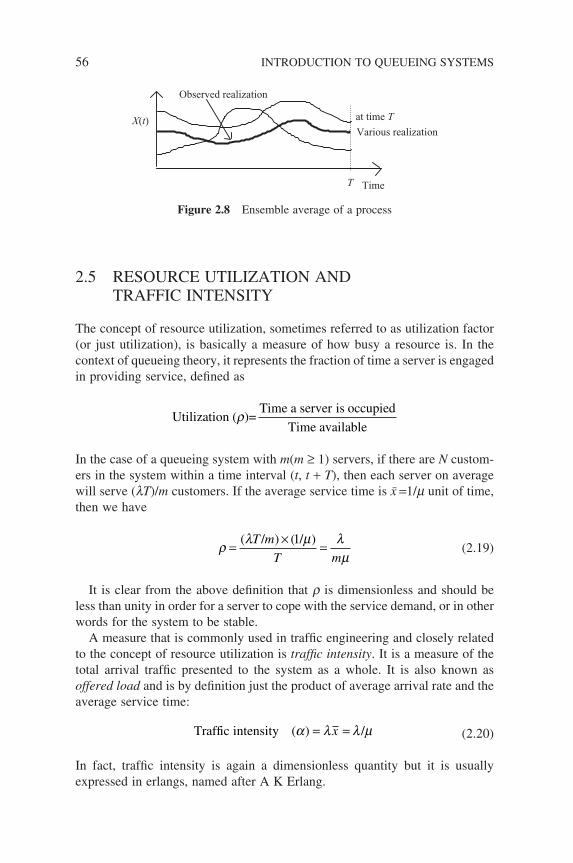
56 INTRODUCTION TO QUEUEING SYSTEMS
2.5 RESOURCE UTILIZATION AND TRAFFIC INTENSITY
The concept of resource utilization, sometimes referred to as utilization factor (or just utilization), is basically a measure of how busy a resource is. In the context of queueing theory, it represents the fraction of time a server is engaged in providing service, defi ned as
Utilization ( )=Time a server is occupied
Time availableρ
In the case of a queueing system with m(m ≥ 1) servers, if there are N custom-ers in the system within a time interval (t, t + T), then each server on average will serve (lT)/m customers. If the average service time is x =1/m unit of time, then we have
ρ λ µ λµ
= × =( / ) ( / )T m
T m
1 (2.19)
It is clear from the above defi nition that r is dimensionless and should be less than unity in order for a server to cope with the service demand, or in other words for the system to be stable.
A measure that is commonly used in traffi c engineering and closely related to the concept of resource utilization is traffi c intensity. It is a measure of the total arrival traffi c presented to the system as a whole. It is also known as offered load and is by defi nition just the product of average arrival rate and the average service time:
Traffic intensity ( ) /α λ λ µ= =x (2.20)
In fact, traffi c intensity is again a dimensionless quantity but it is usually expressed in erlangs, named after A K Erlang.
Various realization
at time T
TimeT
X(t)
Observed realization
Figure 2.8 Ensemble average of a process
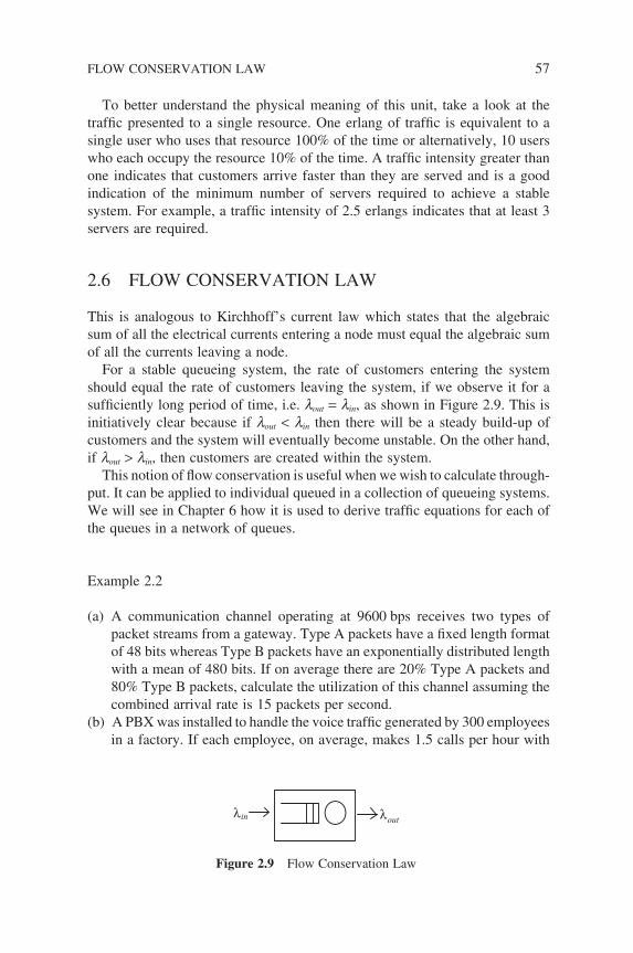
To better understand the physical meaning of this unit, take a look at the traffi c presented to a single resource. One erlang of traffi c is equivalent to a single user who uses that resource 100% of the time or alternatively, 10 users who each occupy the resource 10% of the time. A traffi c intensity greater than one indicates that customers arrive faster than they are served and is a good indication of the minimum number of servers required to achieve a stable system. For example, a traffi c intensity of 2.5 erlangs indicates that at least 3 servers are required.
2.6 FLOW CONSERVATION LAW
This is analogous to Kirchhoff’s current law which states that the algebraic sum of all the electrical currents entering a node must equal the algebraic sum of all the currents leaving a node.
For a stable queueing system, the rate of customers entering the system should equal the rate of customers leaving the system, if we observe it for a suffi ciently long period of time, i.e. lout = lin, as shown in Figure 2.9. This is initiatively clear because if lout < lin then there will be a steady build-up of customers and the system will eventually become unstable. On the other hand, if lout > lin, then customers are created within the system.
This notion of fl ow conservation is useful when we wish to calculate through-put. It can be applied to individual queued in a collection of queueing systems. We will see in Chapter 6 how it is used to derive traffi c equations for each of the queues in a network of queues.
Example 2.2
(a) A communication channel operating at 9600 bps receives two types of packet streams from a gateway. Type A packets have a fi xed length format of 48 bits whereas Type B packets have an exponentially distributed length with a mean of 480 bits. If on average there are 20% Type A packets and 80% Type B packets, calculate the utilization of this channel assuming the combined arrival rate is 15 packets per second.
(b) A PBX was installed to handle the voice traffi c generated by 300 employees in a factory. If each employee, on average, makes 1.5 calls per hour with
λλin out
Figure 2.9 Flow Conservation Law
FLOW CONSERVATION LAW 57
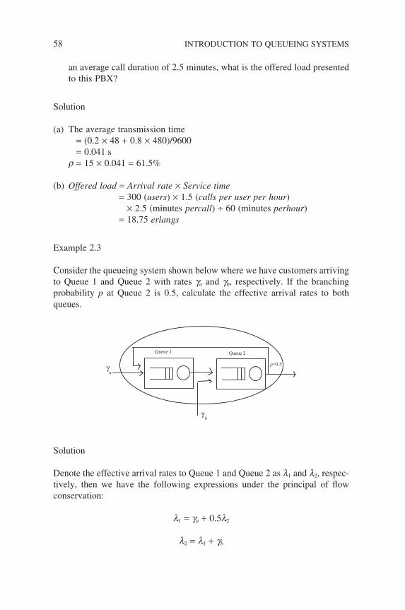
58 INTRODUCTION TO QUEUEING SYSTEMS
an average call duration of 2.5 minutes, what is the offered load presented to this PBX?
Solution
(a) The average transmission time = (0.2 × 48 + 0.8 × 480)/9600 = 0.041 s r = 15 × 0.041 = 61.5%
(b) Offered load = Arrival rate × Service time = 300 (users) × 1.5 (calls per user per hour)
× 2.5 (minutes percall) ÷ 60 (minutes perhour) = 18.75 erlangs
Example 2.3
Consider the queueing system shown below where we have customers arriving to Queue 1 and Queue 2 with rates ga and gb, respectively. If the branching probability p at Queue 2 is 0.5, calculate the effective arrival rates to both queues.
Queue 1 Queue 2
γ
γa
b
p=0.5
Solution
Denote the effective arrival rates to Queue 1 and Queue 2 as l1 and l2, respec-tively, then we have the following expressions under the principal of fl ow conservation:
l1 = ga + 0.5l2
l2 = l1 + gb
Hence, we have
l1 = 2ga + gb
l2 = 2(ga + gb)
2.7 POISSON PROCESS
Poisson process is central to physical process modelling and plays a pivotal role in classical queuing theory. In most elementary queueing systems, the inter-arrival times and service times are assumed to be exponentially distrib-uted or, equivalently, that the arrival and service processes are Poisson, as we shall see below. The reason for its ubiquitous use lies in the fact that it pos-sesses a number of marvellous probabilistic properties that give rise to many elegant queueing results. Secondly, it also closely resembles the behaviour of numerous physical phenomenon and is considered to be a good model for an arriving process that involves a large number of similar and independent users.
Owing to the important role of Poisson process in our subsequent modelling of arrival processes to a queueing system, we will take a closer look at it and examine here some of its marvellous properties.
Put simply, a Poisson process is a counting process for the number of ran-domly occurring point events observed in a given time interval (0, t). It can also be deemed as the limiting case of placing at random k points in the time interval of (0, t). If the random variable X(t) that counts the number of point events in that time interval is distributed according to the well-known Poisson distribution given below, then that process is a Poisson process:
P X t kt
ke
kt[ ( ) ]
( )
!= = −λ λ (2.21)
Here, l is the rate of occurrence of these point events and lt is the mean of a Poisson random variable and physically it represents the average number of occurrences of the event in a time-interval t. Poisson distribution is named after the French mathematician, Simeon Denis Poisson.
2.7.1 The Poisson Process – A Limiting Case
The Poisson process can be considered as a limiting case of the Binomial dis-tribution of a Bernoulli trial. Assuming that the time interval (0, t) is divided into time slots and each time slot contains only one point, if we place points
POISSON PROCESS 59
60 INTRODUCTION TO QUEUEING SYSTEMS
at random in that interval and consider a point in a time slot as a ‘success’, then the number of k ‘successes’ in n time slots is given by the Binomial distribution:
P k nn
kp pk n k[ ( )successes in time-slots] =
− −1
Now let us increase the number of time slots (n) and at the same time decrease the probability (p) of ‘success’ in such a way that the average number of ‘successes’ in a time interval t remains constant at np = lt, then we have the Poisson distribution:
P k t
n
k
t
n
t
nn
k n k
[ )]
(
arrivals in (0,
lim=
−
=
→∞
−λ λ1
λλ λt
k
n n n k
n
t
n
k
n k n
n)
!
( ) ( )lim
. . .lim
→∞ →∞
− − +
−
1 1
1
= −
=
→∞
−−
( )
!
( )
!
λ λ
λ
λ
λ
t
k
t
n
t
k
k
n
n
t
t
k
lim 1
ee t−λ
(2.22)
In the above expression, we made use of the identity:
et
nn
n t
= −
→∞
−
lim 1λ λ
So we see that the process converges to a Poisson process. Therefore, Poisson process can be deemed as the superposition of a large number of Bernoulli arrival processes.
2.7.2 The Poisson Process – An Arrival Perspective
Poisson process has several interpretations and acquires different perspectives depending on which angle we look at it. It can also be viewed as a counting process A(t), t ≥ 0 which counts the number of arrivals up to time t where A(0) = 0. If this counting process satisfi es the following assumptions then it is a Poisson process.
(i) The distribution of the number of arrivals in a time interval depends only on the length of that interval. That is
P A t t o t
P A t t o t
P A t o t
[ ( ) ] ( )
[ ( ) ] ( )
( ) ( )
∆ ∆ ∆∆ ∆ ∆∆ ∆
= = − += = +≥[ ] =
0 1
1
2
λλ
where o(∆t) is a function such that lim∆
∆∆t
o t
t→=
00
( ).
This property is known as independent increments.
(ii) The number of arrivals in non-overlapping intervals is statistically inde-pendent. This property is known as stationary increments.
The result can be shown by examining the change in probability over a time interval (t, t + ∆t). If we defi ne Pk(t) to be the probability of having k arrivals in a time interval t and examine the change in probability in that interval, then
P t t P k arrivals in t t
P k i in t i in t
k
i
k
( ) [ ( )]
[( ) ( ) & ]
+ = +
= − 0=∑
∆ ∆
∆
0
0
,
, (2.23)
Using the assumptions (i) and (ii) given earlier:
P t t P k i arrivals in t P i in t
P t t
ki
k
k
( ) [( ) ( )] [ ]
( )[
+ = − ×
= −=∑∆ ∆
∆0
0
1
,
λ ++ + +−0 01( )] ( )[ ( )]∆ ∆ ∆t P t t tk λ (2.24)
Rearranging the terms, we have
Pk (t + ∆t) − Pk(t) = −l∆tPk(t) + l∆tPk−1(t) + O(∆t)
Dividing both equations by ∆t and letting ∆t → 0, we arrive at
dP t
dtP t P t kk
k k( )
( ) ( )= − + >−λ λ 1 0 (2.25)
Using the same arguments, we can derive the initial condition:
dP t
dtP t0
0( )
( )= −λ (2.26)
POISSON PROCESS 61
62 INTRODUCTION TO QUEUEING SYSTEMS
From the example in Chapter 1, we see that the solution to these two differential equations is given by
P e t0 0( ) = −λ (2.27)
P tt
kek
kt( )
( )
!= −λ λ (2.28)
which is the Poisson distribution. A sample family of Poisson distributions for k = 0, 1, 2 and 3 are plotted in Figure 2.10. The x-axis T = lt.
2.8 PROPERTIES OF THE POISSON PROCESS
2.8.1 Superposition Property
The superposition property says that if k independent Poisson processes A1, A2, . . . Ak are combined into a single process A = A1 + A2 + . . . + Ak, then A is still Poisson with rate l equal to the sum of the individual rates li of Ai, as shown in Figure 2.11.
Recall that the z-transform of a Poisson distribution with parameter lt is e−lt(1−z).
Since A = A1 + A2 + . . . + Ak
k=0
1
Poi
sson
Fun
ctio
n
0.8
0.6
0.4
0.2
00 1 2 3 4 5 6 7
k=1
k=2
k=3
T
Figure 2.10 Sample Poisson distributuon Function
Taking expectations of both sides, we have
E z E Z
E z E z E z
A A A A
A A A
K
k
[ ] = [ ]= [ ] [ ] [ ]
+ + +1 2
1 2
...
. . . . (indenpendencee assumption)
==
− − − −
− + + +
e e
e
t z t z
t
k
k
λ λ
λ λ λ
1
1 2
1 1( ) ( )
( ... ) (
. . . .11−z)
(2.29)
The right-hand side of the fi nal expression is the z-transform of a Poisson distribution with rate (l1 + l2 + . . . + lk), hence the resultant process is Poisson.
2.8.2 Decomposition Property
The decomposition property is just the reverse of the previous property, as shown in Figure 2.12, where a Poisson process A is split into k processes using probability pi (i = 1, . . . , k).
Let us derive the probability mass function of a typical process Ai. On condi-tion that there are N arrivals during the time interval (0, t) from process A, the probability of having k arrivals at process Ai is given by
Poisson A1
Poisson Ak
Poisson A
Figure 2.11 Superposition property
Poisson A1
Poisson Ak
Poisson AP1
Pk
Figure 2.12 Decomposition property
PROPERTIES OF THE POISSON PROCESS 63
64 INTRODUCTION TO QUEUEING SYSTEMS
P A t k A t N N kN
kP pi i
ki
N k[ ( ) | ( ) & ] ( )= = ≥ =
− −1 (2.30)
The unconditional probability is then calculated using the total probability theorem:
P A t kN
N k kp p
t
Ne
e
k
p
iN k
ki
N kN
t
ti
[ ( ) ]!
( )! !( )
( )
!
!
= =−
−
=
=
∞− −
−
∑ 1 1λ λ
λ
11
1
11
−
−−
=−
−
=
∞
−
∑p
p t
N k
e
k
p
p
i
k
N k
iN
ti
i
k
[( ) ]
( )!
![(
λ
λ
pp tp t
j
p t
ke
ik
j
ij
ik
p ti
) ][( ) ]
!
( )
!
λ λ
λ λ
=
∞
−
∑ −
=
0
1
(2.31)
That is, a Poisson process with rate pil.
2.8.3 Exponentially Distributed Inter-arrival Times
The exponential distribution and the Poisson process are closely related and in fact they mirror each other in the following sense. If the inter-arrival times in a point process are exponentially distributed, then the number of arrival points in a time interval is given by the Poisson distribution and the process is a Poisson arrival process. Conversely, if the number of arrival points in any interval is a Poisson random variable, the inter-arrival times are exponential distributed and the arrival process is Poisson.
Let t be the inter-arrival time, then
P[t ≤ t] = 1 − P[t > t].
But P[t > t] is just the probability that no arrival occurs in (0, t); i.e. P0(t). Therefore we obtain
P t e t[ ] (τ λ≤ = − −1 exponential distribution) (2.32)
2.8.4 Memoryless (Markovian) Property of Inter-arrival Times
The memoryless property of a Poisson process means that if we observe the process at a certain point in time, the distribution of the time until next arrival is not affected by the fact that some time interval has passed since the last
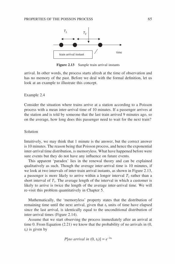
arrival. In other words, the process starts afresh at the time of observation and has no memory of the past. Before we deal with the formal defi nition, let us look at an example to illustrate this concept.
Example 2.4
Consider the situation where trains arrive at a station according to a Poisson process with a mean inter-arrival time of 10 minutes. If a passenger arrives at the station and is told by someone that the last train arrived 9 minutes ago, so on the average, how long does this passenger need to wait for the next train?
Solution
Intuitively, we may think that 1 minute is the answer, but the correct answer is 10 minutes. The reason being that Poisson process, and hence the exponential inter-arrival time distribution, is memoryless. What have happened before were sure events but they do not have any infl uence on future events.
This apparent ‘paradox’ lies in the renewal theory and can be explained qualitatively as such. Though the average inter-arrival time is 10 minutes, if we look at two intervals of inter-train arrival instants, as shown in Figure 2.13, a passenger is more likely to arrive within a longer interval T2 rather than a short interval of T1. The average length of the interval in which a customer is likely to arrive is twice the length of the average inter-arrival time. We will re-visit this problem quantitatively in Chapter 5.
Mathematically, the ‘memoryless’ property states that the distribution of remaining time until the next arrival, given that t0 units of time have elapsed since the last arrival, is identically equal to the unconditional distribution of inter-arrival times (Figure 2.14).
Assume that we start observing the process immediately after an arrival at time 0. From Equation (2.21) we know that the probability of no arrivals in (0, t0) is given by
P[no arrival in (0, t0)] = e−lt0
time
T1 T2
train arrival instant
Figure 2.13 Sample train arrival instants
PROPERTIES OF THE POISSON PROCESS 65
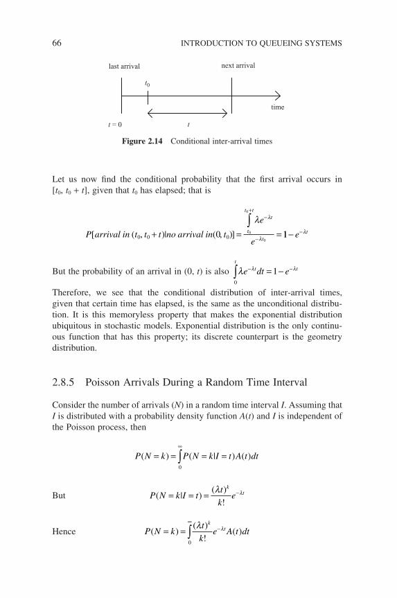
66 INTRODUCTION TO QUEUEING SYSTEMS
Let us now fi nd the conditional probability that the fi rst arrival occurs in [t0, t0 + t], given that t0 has elapsed; that is
P arrival in t t t no arrival in t
e
et
t tt
t[ ( )| ( )]0 0 00 0
0
0, ,+ = =
+−
−
∫ λ λ
λ 11− −e tλ
But the probability of an arrival in (0, t) is also 0
1t
t te dt e∫ − −= −λ λ λ
Therefore, we see that the conditional distribution of inter-arrival times, given that certain time has elapsed, is the same as the unconditional distribu-tion. It is this memoryless property that makes the exponential distribution ubiquitous in stochastic models. Exponential distribution is the only continu-ous function that has this property; its discrete counterpart is the geometry distribution.
2.8.5 Poisson Arrivals During a Random Time Interval
Consider the number of arrivals (N) in a random time interval I. Assuming that I is distributed with a probability density function A(t) and I is independent of the Poisson process, then
P N k P N k I t A t dt( ) ( | ) ( )= = = =∞
∫0
But P N k I tt
ke
kt( | )
( )
!= = = −λ λ
Hence P N kt
ke A t dt
kt( )
( )
!( )= =
∞−∫
0
λ λ
last arrival next arrival
t = 0
t0
t
time
Figure 2.14 Conditional inter-arrival times
Taking the z-transform, we obtain
N zt
ke A t dt z
etz
k
k
kt k
t
k
k
( )( )
!( )
( )
=
=
=
∞ ∞−
∞−
=
∞
∑ ∫
∫ ∑
0 0
0 0
λ
λ
λ
λ
!!( )
( )
)
)
A t dt
e A t dt
A z
z t=
= −
∞−( −∫
0
λ λ
λ λ*(
where A*(l − lz) is the Laplace transform of the arrival distribution evaluated at the point (l − lz).
Example 2.5
Let us consider again the problem presented in Example 2.4. When this pas-senger arrives at the station:
a) What is the probability that he will board a train in the next 5 minutes?b) What is the probability that he will board a train in 5 to 9 minutes?
Solution
a) From Example 2.4, we have l = 1/10 = 0.1 min−1, hence for a time period of 5 minutes we have
λλλ
t
P train ine t
k
et k
= × =
= = =− −
5 0 1 0 5
0 50 5
00
0 5 0
. .
[( )
!
( . )
!
.
and
min] ..607
He will board a train if at least one train arrives in 5 minutes; hence
P[at least 1 train in 5 min] = 1 − P[0 train in 5 min]= 0.393
b) He will need to wait from 5 to 9 minutes if no train arrives in the fi rst 5 minutes and board a train if at least one train arrives in the time interval 5 to 9 minutes. From (a) we have
P[0 train in 5 min] = 0.607
PROPERTIES OF THE POISSON PROCESS 67
68 INTRODUCTION TO QUEUEING SYSTEMS
and P[at least 1 train in next 4 min] = 1 − P[0 train in next 4 min]
= − =−
10 4
00 33
0 4 0e . ( . )
!.
Hence, P[0 train in 5 min & at least 1 train in next 4 min]= P[0 train in 5 min] × P[at least 1 train in next 4 min]= 0.607 × 0.33 = 0.2
Example 2.6
Pure Aloha is a packet radio network, originated at the University of Hawaii, that provides communication between a central computer and various remote data terminals (nodes). When a node has a packet to send, it will transmit it immediately. If the transmitted packet collides with other packets, the node concerned will re-transmit it after a random delay t. Calculate the throughput of this pure Aloha system.
Solution
For simplicity, let us make the following assumptions:
(i) The packet transmission time is one (one unit of measure).(ii) The number of nodes is large, hence the total arrival of packets from all
nodes is Poisson with rate l.(iii) The random delay t is exponentially distributed with density function
be−bt, where b is the node’s retransmission attempt rate.
Given these assumptions, if there are n node waiting for the channel to re-transmit their packets, then the total packet arrival presented to the channel can be assumed to be Poisson with rate (l + nb) and the throughput S is then given by
S = (l + nb)P[a successful transmission]= (l + nb)Psucc
From Figure 2.15, we see that there will be no packet collision if there is only one packet arrival within two units of time. Since the total arrival of packets is assumed to be Poisson, we have
Psucc = e−2(l+nb)
and hence
S = (l + nb)e−2(l+nb)
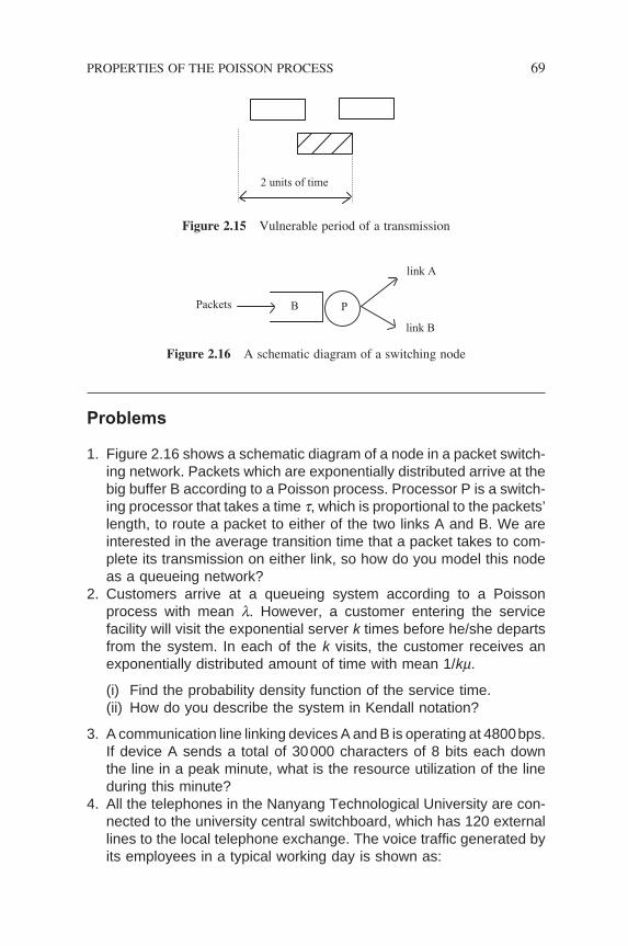
Problems
1. Figure 2.16 shows a schematic diagram of a node in a packet switch-ing network. Packets which are exponentially distributed arrive at the big buffer B according to a Poisson process. Processor P is a switch-ing processor that takes a time t, which is proportional to the packets’ length, to route a packet to either of the two links A and B. We are interested in the average transition time that a packet takes to com-plete its transmission on either link, so how do you model this node as a queueing network?
2. Customers arrive at a queueing system according to a Poisson process with mean l. However, a customer entering the service facility will visit the exponential server k times before he/she departs from the system. In each of the k visits, the customer receives an exponentially distributed amount of time with mean 1/km.
(i) Find the probability density function of the service time.(ii) How do you describe the system in Kendall notation?
3. A communication line linking devices A and B is operating at 4800 bps. If device A sends a total of 30 000 characters of 8 bits each down the line in a peak minute, what is the resource utilization of the line during this minute?
4. All the telephones in the Nanyang Technological University are con-nected to the university central switchboard, which has 120 external lines to the local telephone exchange. The voice traffi c generated by its employees in a typical working day is shown as:
2 units of time
Figure 2.15 Vulnerable period of a transmission
Packets
link A
link B
B P
Figure 2.16 A schematic diagram of a switching node
PROPERTIES OF THE POISSON PROCESS 69
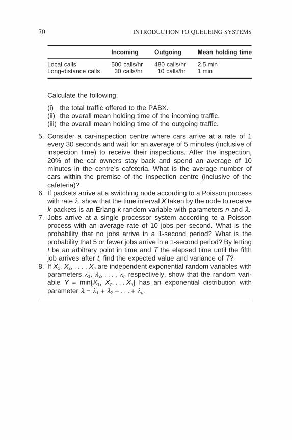
70 INTRODUCTION TO QUEUEING SYSTEMS
Incoming Outgoing Mean holding time
Local calls 500 calls/hr 480 calls/hr 2.5 minLong-distance calls 30 calls/hr 10 calls/hr 1 min
Calculate the following:
(i) the total traffi c offered to the PABX.(ii) the overall mean holding time of the incoming traffi c.(iii) the overall mean holding time of the outgoing traffi c.
5. Consider a car-inspection centre where cars arrive at a rate of 1 every 30 seconds and wait for an average of 5 minutes (inclusive of inspection time) to receive their inspections. After the inspection, 20% of the car owners stay back and spend an average of 10 minutes in the centre’s cafeteria. What is the average number of cars within the premise of the inspection centre (inclusive of the cafeteria)?
6. If packets arrive at a switching node according to a Poisson process with rate l, show that the time interval X taken by the node to receive k packets is an Erlang-k random variable with parameters n and l.
7. Jobs arrive at a single processor system according to a Poisson process with an average rate of 10 jobs per second. What is the probability that no jobs arrive in a 1-second period? What is the probability that 5 or fewer jobs arrive in a 1-second period? By letting t be an arbitrary point in time and T the elapsed time until the fi fth job arrives after t, fi nd the expected value and variance of T?
8. If X1, X2, . . . , Xn are independent exponential random variables with parameters l1, l2, . . . , ln respectively, show that the random vari-able Y = minX1, X2, . . . Xn has an exponential distribution with parameter l = l1 + l2 + . . . + ln.
3Discrete and Continuous Markov Processes
In Chapter 2, we derived Little’s theorem which gives us a basic means to study performance measures of a queueing system. Unfortunately, if we take a closer look at this expression, the only quantity that we have prior knowledge of is probably the average arrival rate. The other two quantities are generally unknown and they are exactly what we want to determine for that particular queueing system.
To exploit the full potential of Little’s theorem, we need other means to calculate either one of the two quantities. It turns out that it is easier to deter-mine N as the number of customers in a queueing system that can be modelled as a continuous-time Markov process, a concept that we will study in this chapter. Once the probability mass function of the number of customers in a queueing system is obtained using the Markov chain, the long-term average N can then be easily computed.
Before we embark on the theory of Markov processes, let us look at the more general random processes – the so-called stochastic processes. The Markov process is a special class of stochastic processes that exhibits particular kinds of dependencies among the random variables within the same process. It pro-vides the underlying theory of analysing queueing systems. In fact, each queue-ing system can, in principle, be mapped onto an instance of a Markov process or its variants (e.g. Imbedded Markov process) and mathematically analysed. We shall discuss this in detail later in the chapter.
Queueing Modelling Fundamentals Second Edition Ng Chee-Hock and Soong Boon-Hee© 2008 John Wiley & Sons, Ltd
72 DISCRETE AND CONTINUOUS MARKOV PROCESSES
3.1 STOCHASTIC PROCESSES
Simply put, a stochastic process is a mathematical model for describing an empirical process that changes with an index, which is usually the time in most of the real-life processes, according to some probabilistic forces. More specifi -cally, a stochastic process is a family of random variables X(t), t ∈ T defi ned on some probability space and indexed by a parameter tt ∈ T, where t is usually called the time parameter. The probability that X(t) takes on a value, say i and that is P[X(t) = i], is the range of that probability space.
In our daily life we encounter many stochastic processes. For example, the price Pst(t) of a particular stock counter listed on the Singapore stock exchange as a function of time is a stochastic process. The fl uctuations in Pst(t) through-out the trading hours of the day can be deemed as being governed by probabi-listic forces and hence a stochastic process. Another example will be the number of customers calling at a bank as a function of time.
Basically, there are three parameters that characterize a stochastic process:
(1) State spaceThe values assumed by a random variable X(t) are called ‘states’ and the col-lection of all possible values forms the ‘state space’ of the process. If X(t) = i then we say the process is in state i. In the stock counter example, the state space is the set of all prices of that particular counter throughout the day.
If the state space of a stochastic process is fi nite or at most countably infi nite, it is called a ‘discrete-state’ process, or commonly referred to as a stochastic chain. In this case, the state space is often assumed to be the non-negative integers 0, 1, 2, . . .. The stock counter example mentioned above is a dis-crete-state stochastic chain since the price fl uctuates in steps of few cents or dollars.
On the other hand, if the state space contains a fi nite or infi nite interval of the real numbers, then we have a ‘continuous-state’ process. At this juncture, let us look at a few examples about the concept of ‘countable infi nite’ without going into the mathematics of set theory. For example, the set of positive integer numbers n in the interval [a, b] is fi nite or countably infi nite, whereas the set of real numbers in the same interval [a, b] is infi nite.
In the subsequent study of queueing theory, we are going to model the number of customers in a queueing system at a particular time as a Markov chain and the state represents the actual number of customers in the system. Hence we will restrict our discussion to the discrete-space stochastic processes.
(2) Index parameterAs mentioned above, the index is always taken to be the time parameter in the context of applied stochastic processes. Similar to the state space, if a process changes state at discrete or fi nite countable time instants, we have a
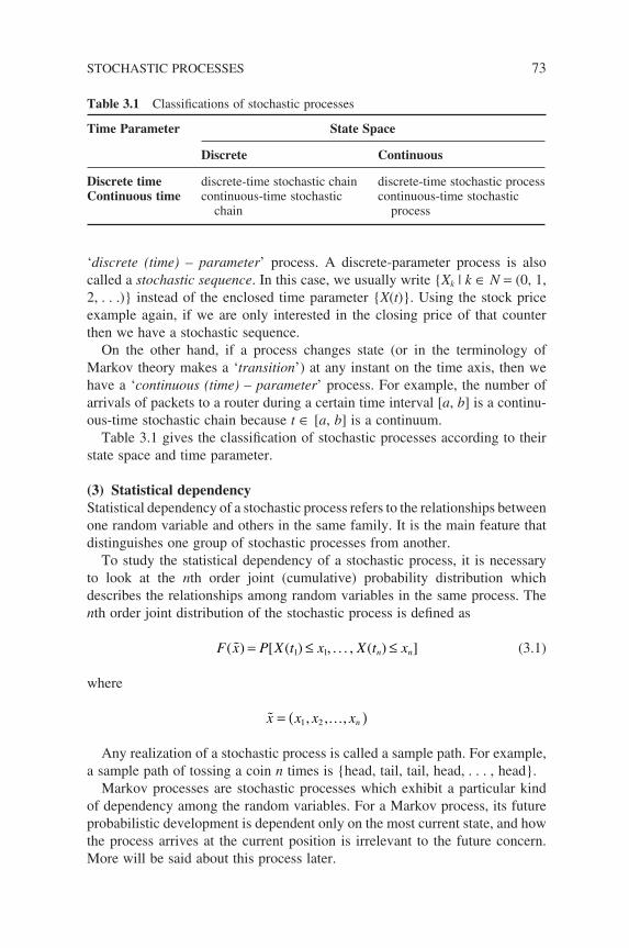
‘discrete (time) – parameter’ process. A discrete-parameter process is also called a stochastic sequence. In this case, we usually write Xk | k ∈ N = (0, 1, 2, . . .) instead of the enclosed time parameter X(t). Using the stock price example again, if we are only interested in the closing price of that counter then we have a stochastic sequence.
On the other hand, if a process changes state (or in the terminology of Markov theory makes a ‘transition’) at any instant on the time axis, then we have a ‘continuous (time) – parameter’ process. For example, the number of arrivals of packets to a router during a certain time interval [a, b] is a continu-ous-time stochastic chain because t ∈ [a, b] is a continuum.
Table 3.1 gives the classifi cation of stochastic processes according to their state space and time parameter.
(3) Statistical dependencyStatistical dependency of a stochastic process refers to the relationships between one random variable and others in the same family. It is the main feature that distinguishes one group of stochastic processes from another.
To study the statistical dependency of a stochastic process, it is necessary to look at the nth order joint (cumulative) probability distribution which describes the relationships among random variables in the same process. The nth order joint distribution of the stochastic process is defi ned as
F x P X t x X t xn n( ) [ ( ) ( ) ] = ≤ ≤1 1, . . . , (3.1)
where
…x x x xn= ( )1 2, , ,
Any realization of a stochastic process is called a sample path. For example, a sample path of tossing a coin n times is head, tail, tail, head, . . . , head.
Markov processes are stochastic processes which exhibit a particular kind of dependency among the random variables. For a Markov process, its future probabilistic development is dependent only on the most current state, and how the process arrives at the current position is irrelevant to the future concern. More will be said about this process later.
Table 3.1 Classifi cations of stochastic processes
Time Parameter State Space
Discrete Continuous
Discrete time discrete-time stochastic chain discrete-time stochastic processContinuous time continuous-time stochastic
chaincontinuous-time stochastic
process
STOCHASTIC PROCESSES 73
74 DISCRETE AND CONTINUOUS MARKOV PROCESSES
In the study of stochastic processes, we are generally interested in the prob-ability that X(t) takes on a value i at some future time t, that is P[X(t) = i], because precise knowledge cannot be had about the state of the process in future times. We are also interested in the steady state probabilities if the prob-ability converges.
Example 3.1
Let us denote the day-end closing price of a particular counter listed on the Singapore stock exchange on day k as Xk. If we observed the following closing prices from day k to day k + 3, then the following observed sequence Xk is a stochastic sequence:
X X
X X
k k
k k
= =
= =
+
+ +
$ . $ .
$ . $ .
2 45 2 38
2 29 2 78
1
2 3
However, if we are interested in the fl uctuations of prices during the trading hours and assume that we have observed the following prices at the instants t1 < t2 < t3 < t4, then the chain X(t) is a continuous-time stochastic chain:
X t X t
X t X t
( ) $ . ( ) $ .
( ) $ . ( ) $ .
1 2
3 4
2 38 2 39
2 40 2 36
= =
= =
3.2 DISCRETE-TIME MARKOV CHAINS
The discrete-time Markov chain is easier to conceptualize and it will pave the way for our later introduction of the continuous Markov processes, which are excellent models for the number of customers in a queueing system.
As mentioned in Section 3.1, a Markov process is a stochastic process which exhibits a simple but very useful form of dependency among the random vari-ables of the same family, namely the dependency that each random variable in the family has a distribution that depends only on the immediate preceding random variable. This particular type of dependency in a stochastic process was fi rst defi ned and investigated by the Russian mathematician Andrei A Markov and hence the name Markov process, or Markov chain if the state space is discrete. In the following sections we will be merely dealing with only the discrete-state Markov processes; we will use Markov chain or process inter-changeably without fear of confusion.
As an illustration to the idea of a Markov chain vs a stochastic process, let us look at a coin tossing experiment. Firstly, let us defi ne two random variables; namely Xk = 1 (or 0) when the outcome of the kth trial is a ‘head’ (or tail), and Yk = accumulated number of ‘heads’ so far. Assuming the system starts in state
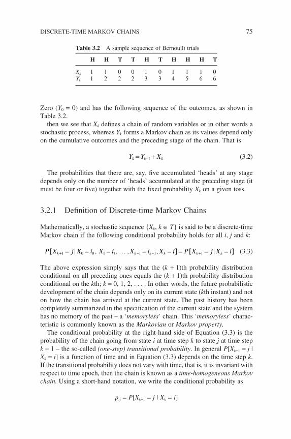
Zero (Y0 = 0) and has the following sequence of the outcomes, as shown in Table 3.2.
then we see that Xk defi nes a chain of random variables or in other words a stochastic process, whereas Yk forms a Markov chain as its values depend only on the cumulative outcomes and the preceding stage of the chain. That is
Y Y Xk k k= +−1 (3.2)
The probabilities that there are, say, fi ve accumulated ‘heads’ at any stage depends only on the number of ‘heads’ accumulated at the preceding stage (it must be four or fi ve) together with the fi xed probability Xk on a given toss.
3.2.1 Defi nition of Discrete-time Markov Chains
Mathematically, a stochastic sequence Xk, k ∈ T is said to be a discrete-time Markov chain if the following conditional probability holds for all i, j and k:
P X j X i X i X i X i P X j X ik k k k k k+ − − += = = = =[ ] = = =[ ]1 0 0 1 1 1 1 1, , , ,… (3.3)
The above expression simply says that the (k + 1)th probability distribution conditional on all preceding ones equals the (k + 1)th probability distribution conditional on the kth; k = 0, 1, 2, . . . . In other words, the future probabilistic development of the chain depends only on its current state (kth instant) and not on how the chain has arrived at the current state. The past history has been completely summarized in the specifi cation of the current state and the system has no memory of the past – a ‘memoryless’ chain. This ‘memoryless’ charac-teristic is commonly known as the Markovian or Markov property.
The conditional probability at the right-hand side of Equation (3.3) is the probability of the chain going from state i at time step k to state j at time step k + 1 – the so-called (one-step) transitional probability. In general P[Xk+1 = j | Xk = i] is a function of time and in Equation (3.3) depends on the time step k. If the transitional probability does not vary with time, that is, it is invariant with respect to time epoch, then the chain is known as a time-homogeneous Markov chain. Using a short-hand notation, we write the conditional probability as
pij = P[Xk+1 = j | Xk = i]
Table 3.2 A sample sequence of Bernoulli trials
H H T T H T H H H T
Xk 1 1 0 0 1 0 1 1 1 0Yk 1 2 2 2 3 3 4 5 6 6
DISCRETE-TIME MARKOV CHAINS 75
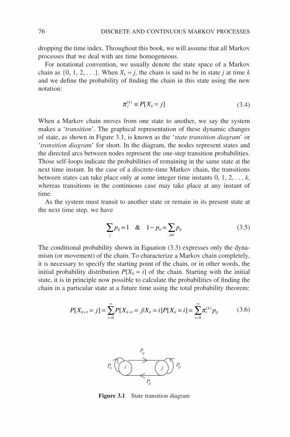
76 DISCRETE AND CONTINUOUS MARKOV PROCESSES
dropping the time index. Throughout this book, we will assume that all Markov processes that we deal with are time homogeneous.
For notational convention, we usually denote the state space of a Markov chain as 0, 1, 2, . . .. When Xk = j, the chain is said to be in state j at time k and we defi ne the probability of fi nding the chain in this state using the new notation:
π jk
kP X j( ) [ ]≡ = (3.4)
When a Markov chain moves from one state to another, we say the system makes a ‘transition’. The graphical representation of these dynamic changes of state, as shown in Figure 3.1, is known as the ‘state transition diagram’ or ‘transition diagram’ for short. In the diagram, the nodes represent states and the directed arcs between nodes represent the one-step transition probabilities. Those self-loops indicate the probabilities of remaining in the same state at the next time instant. In the case of a discrete-time Markov chain, the transitions between states can take place only at some integer time instants 0, 1, 2, . . . k, whereas transitions in the continuous case may take place at any instant of time.
As the system must transit to another state or remain in its present state at the next time step, we have
j
ij iij i
ijp p p∑ ∑= − =≠
1 1& (3.5)
The conditional probability shown in Equation (3.3) expresses only the dyna-mism (or movement) of the chain. To characterize a Markov chain completely, it is necessary to specify the starting point of the chain, or in other words, the initial probability distribution P[X0 = i] of the chain. Starting with the initial state, it is in principle now possible to calculate the probabilities of fi nding the chain in a particular state at a future time using the total probability theorem:
P X j P X j X i P X i pki
k k ki
ik
ij[ ] [ | ] [ ] ( )+
=
∞
+=
∞
= = = = = =∑ ∑10
10
π (3.6)
Pii
Pji
i j Pjj
Pij
Figure 3.1 State transition diagram
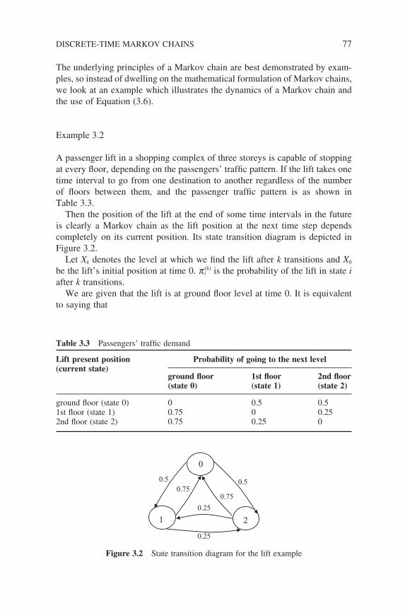
The underlying principles of a Markov chain are best demonstrated by exam-ples, so instead of dwelling on the mathematical formulation of Markov chains, we look at an example which illustrates the dynamics of a Markov chain and the use of Equation (3.6).
Example 3.2
A passenger lift in a shopping complex of three storeys is capable of stopping at every fl oor, depending on the passengers’ traffi c pattern. If the lift takes one time interval to go from one destination to another regardless of the number of fl oors between them, and the passenger traffi c pattern is as shown in Table 3.3.
Then the position of the lift at the end of some time intervals in the future is clearly a Markov chain as the lift position at the next time step depends completely on its current position. Its state transition diagram is depicted in Figure 3.2.
Let Xk denotes the level at which we fi nd the lift after k transitions and X0 be the lift’s initial position at time 0. p i
(k) is the probability of the lift in state i after k transitions.
We are given that the lift is at ground fl oor level at time 0. It is equivalent to saying that
Table 3.3 Passengers’ traffi c demand
Lift present position(current state)
Probability of going to the next level
ground fl oor(state 0)
1st fl oor(state 1)
2nd fl oor(state 2)
ground fl oor (state 0) 0 0.5 0.51st fl oor (state 1) 0.75 0 0.252nd fl oor (state 2) 0.75 0.25 0
1 2
0
0.50.5
0.25
0.25
0.750.75
Figure 3.2 State transition diagram for the lift example
DISCRETE-TIME MARKOV CHAINS 77
78 DISCRETE AND CONTINUOUS MARKOV PROCESSES
p00 ≡ P(X0 = 0) = 1
p 01 ≡ P(X0 = 1) = 0
p02 ≡ P(X0 = 2) = 0
Or in vector form
p (0) = [p 00, p 0
1, p 02] = [1, 0, 0]
(i) The probability of the lift’s position after 1st transition:
π
π
01
1
1 0 0
11
0
0
1 0 0 0 5 0 0 5 0
= =
= = = =
= × + × + × =
≡
∑P X
P X X i P X i
P X
i
( )
( | ) ( )
. .
( 11
1 0 0
1
1
0 5
=
= = = =
=
∑)
( | ) ( )
.i
P X X i P X i
Similarly
p12 = P(X1 = 2) = 0.5
(ii) The probability of the lift’s position after 2nd transition:
π02
2
2 1 1
0
0
0 0 0 75 0 5 0 75 0 50
≡ =
= = = =
= × + × + ×=
∑P X
P X X i P X ii
( )
( | ) ( )
. . . ..775
and
p 21 = P(X2 = 1) = 0.125
p 22 = P(X2 = 2) = 0.125
From the above calculations, we see that we need only the probabilities of the lift’s position after the 1st transition in order to calculate its probabilities after the 2nd transition. That is to say that the future development of the process depends only on its current position.
3.2.2 Matrix Formulation of State Probabilities
Students who have refreshed their memory of matrices in Chapter 1 will rec-ognize that the above calculations can be formulated more succinctly in terms of matrix operations. Let us express the transition probabilities in an n × n square matrix P, assuming there are n states. The square matrix is known as transition probability matrix, or transition matrix for short:
P p
p p p
p p p
p
p
ij
n
n
ij
nn
= =
( )
11 12 1
21 22 2 (3.7)
The element pij is the transition probability defi ned in Equation (3.3). If the number of states is fi nite, say n, then we have a n x n matrix P, otherwise the matrix is infi nite. Since the probability of going to all other states, including itself, should sum to unity, as shown in Equation (3.5), the sum of each row in the above matrix should equal to unity, that is:
jijp∑ = 1
A matrix with each row sums to unity and all elements positive or zero are called a stochastic matrix. A Markov chain is completely characterized by this (one-step) transition probability matrix together with the initial probability vector.
Similarly, we express the state probabilities at each time interval as a row vector:
π π π π( ) ( ) ( ) ( )( )k k knk= 0 1, , . . . , (3.8)
Using these matrix notations, the calculations shown in Example 3.2 can be formulated as
π ππ π
π π
( ) ( )
( ) ( )
( ) ( )
1 0
2 1
1
=
=
= −
P
P
Pk k
. . .
(3.9)
Back substituting the p (i), we have from Equation (3.9) the following equation:
π π( ) ( ) ( )k kP= 0 (3.10)
DISCRETE-TIME MARKOV CHAINS 79
80 DISCRETE AND CONTINUOUS MARKOV PROCESSES
where
P P P Pk k k( ) ( )= ⋅ =−1 (3.11)
Pk, the so-called k-step transition matrix, is the k-fold multiplication of the one-step transition matrix by itself. We defi ne P(0) = I.
Equations (3.10) and (3.11) give us a general method for calculating the state probability k steps into a chain. From matrix operations, we know that
P P Pk l k l( ) ( ) ( )+ = × (3.12)
or
P P Pijk l
k
n
ikk
kjl+
=
= ∑0
(3.13)
These two equations are the well-known Chapman–Kolmogorov forward equations.
Example 3.3
For the lift example, the transition probability matrix is
P =
0 0 5 0 5
0 75 0 0 25
0 75 0 25 0
. .
. .
. .
The transition matrices for the fi rst few transitions can be computed as
P P P( ) ( ) ( )
. . .
. . .
. .
2 1 1
0 75 0 125 0 125
0 1875 0 4375 0 375
0 1875 0 3
= × =775 0 4375
0 1875 0 4063 0 4062
0 6094 0 1875 0 2033
.
. . .
. . .( )
=P 11
0 6094 0 2031 0 1875
0 6094 0 1953 0 1953
0 21934
. . .
. . .
.( )
=P 00 0 3555 0 3515
0 2930 0 3515 0 3554
. .
. . .
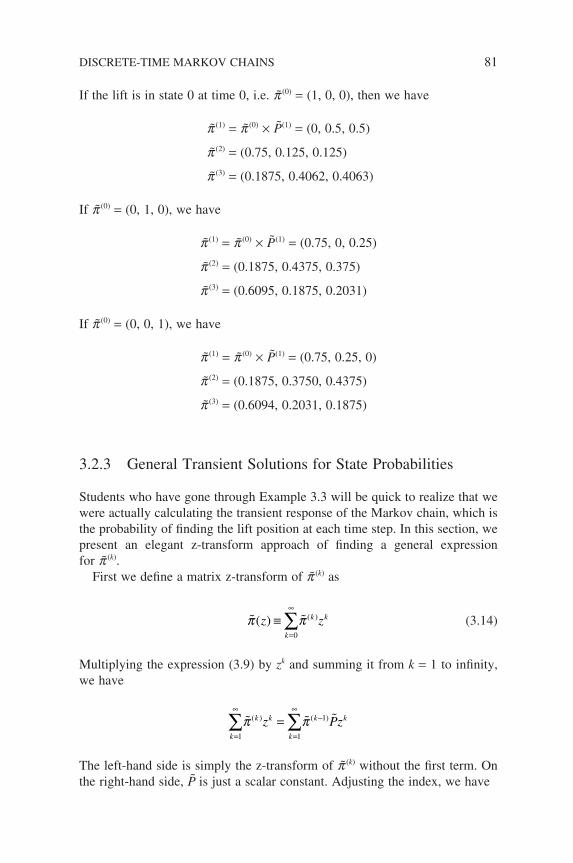
If the lift is in state 0 at time 0, i.e. p (0) = (1, 0, 0), then we have
p (1) = p (0) × P(1) = (0, 0.5, 0.5)
p (2) = (0.75, 0.125, 0.125)
p (3) = (0.1875, 0.4062, 0.4063)
If p (0) = (0, 1, 0), we have
p (1) = p (0) × P(1) = (0.75, 0, 0.25)
p (2) = (0.1875, 0.4375, 0.375)
p (3) = (0.6095, 0.1875, 0.2031)
If p (0) = (0, 0, 1), we have
p (1) = p (0) × P(1) = (0.75, 0.25, 0)
p (2) = (0.1875, 0.3750, 0.4375)
p (3) = (0.6094, 0.2031, 0.1875)
3.2.3 General Transient Solutions for State Probabilities
Students who have gone through Example 3.3 will be quick to realize that we were actually calculating the transient response of the Markov chain, which is the probability of fi nding the lift position at each time step. In this section, we present an elegant z-transform approach of fi nding a general expression for p (k).
First we defi ne a matrix z-transform of p (k) as
π π( ) ( )z zk
k k≡=
∞
∑0
(3.14)
Multiplying the expression (3.9) by zk and summing it from k = 1 to infi nity, we have
k
k k
k
k kz Pz=
∞
=
∞−∑ ∑=
1 1
1 π π( ) ( )
The left-hand side is simply the z-transform of p (k) without the fi rst term. On the right-hand side, P is just a scalar constant. Adjusting the index, we have
DISCRETE-TIME MARKOV CHAINS 81
82 DISCRETE AND CONTINUOUS MARKOV PROCESSES
π π π
π π
( )
( ) ( )
( ) ( )
( )
z zP z
z I zP
k
k k− =
= −
=
∞− −
−
∑0
1
1 1
0 1
(3.15)
where I is the identity matrix and the superscript (−1) denotes the matrix inverse. If the inverse exists, we could obtain the transient solution for the state probability by carrying out the inverse z-transform of Equation (3.15). Com-paring Equations (3.15) and (3.10), we see that the k-step transition matrix is given by
P I zPk = − −( ) 1 (3.16)
Coupling with the initial state probability vector, we can then calculate the state probability vector k-step into the future.
Besides the z-transform method, there is another way of fi nding P(k). Recall from the section on ‘Eigenvalues, Eigenvectors and Spectral Representation’ in Chapter 1, if the eigenvalues li of P are all distinct, then P(k) can be expressed as
P N NB B B
k k
k knk
n
( ) == + +
−Λ 1
1 1 2 2λ λ λ. . .
(3.17)
where N is a matrix that makes up of the eigenvectors of P, and Bi are matrices defi ned in that section. Students should not mistakenly think that this is an easier way of computing P(k). It is in general quite diffi cult to compute the eigenvalues and eigenvectors of a matrix.
Example 3.4
Returning to the lift example, let us fi nd the explicit solution for p (k). First we fi nd the matrix (I − zP):
( ) I zP
z z
z z
z z
− =
− −
− −
− −
11
2
1
23
41
1
43
4
1
41
, ,
, , ,
, ,

To fi nd the inverse, we need to fi nd the determinant of the matrix:
∆
∆
≡ −
≡ − =
− −
− −
−
det
det det
, ,
, , ,
( ):
( )
I zP
I zP
z z
z z
z
11
2
1
23
41
1
43
4,, ,−
= − +
+
1
41
1 11
41
3
4
z
z z z( )
and the inverse of (I − zP) is given by
( ) I zP
z z z z z
z z z z− =
− + +
+ −−1
2 2 2
2 21
11
16
1
2
1
8
1
2
1
83
4
3
161
3
8
1
4∆
, ,
, , ++
+ + −
3
83
4
3
16
1
4
3
81
3
8
2
2 2 2
z
z z z z z, ,
Carrying out partial fraction and grouping the result into three matrices, we obtain
( ) I zPz z
− =−
+
+
−1
17
1
3 2 2
3 2 2
3 2 2
1
114
0 0 0
01
2
1
2
01
2
1
2
++
− −
−
−
17
134
4 2 2
33
2
3
2
33
2
3
2
z
P k ( ) ==
+ −
1
7
3 2 2
3 2 2
3 2 2
1
4
0 0 0
01
2
1
2
01
2
1
2
k
+ −
− −
−
−
1
7
3
4
4 2 2
33
2
3
2
33
2
3
2
k
Once the k-step transition matrix is obtained, we can then calculate the transient solution using p (k) = p (0)P(k).
DISCRETE-TIME MARKOV CHAINS 83
84 DISCRETE AND CONTINUOUS MARKOV PROCESSES
Example 3.5
Now, let us use the spectrum representation method to fi nd the explicit solution for P(k). First we have to fi nd the eigenvalues and eigenvectors of the transition probability matrix:
P =
0 0 5 0 5
0 75 0 0 25
0 75 0 25 0
. .
. .
. .
The eigenvalues can be found by solving the equation det(P − lI) = 0. Forming the necessary matrix and taking the determinant, we have
(l − 1)(4l + 3)(4l + 1) = 0
Now it remains for us to fi nd the corresponding eigenvectors. For l = 1, the corresponding eigenvector (f1) can be found by solving the following set of simultaneous equations:
0 0 5 0 5
0 75 0 0 25
0 75 0 25 0
11
2
3
1
2
3
. .
. .
. .
( )
=
x
x
x
x
x
x
Similarly, the other eigenvectors (f2 and f3) can be found using the same method and we have
N = −− −
= −−
1 1 3 0
1 1 4 1
1 1 4 1
1 0 0
0 3 4 0
0 0 1 4
/
/
/
/
/
and Λ
Finding the inverse of N, we have
N − = − −−
1
3 7 2 7 2 7
12 7 6 7 6 7
0 1 2 1 2
/ / /
/ / /
/ /
Having obtained these matrices, we are ready to form the following matrices:
B x1 1 1
1
1
1
3 7 2 7 2 7
3 7 2 7 2 7
3 7 2 7 2 7
3 7 2
= × =
=π ( / / / )
/ / /
/ / /
/ /77 2 7/
B x3 3 3
1 3
1 4
1 4
12 7 6 7 6 71
7
4 2 2
3 3 2= × = −−
− −( ) =− −
−π/
/
/
/ / / / 33 2
3 3 2 3 2
1
7
4 2 2
3 3 2 3 2
3 3 2 3 2
2
/
/ /
/ /
/ /−
=
− −−−
= B x22 2
0
1
1
0 1 2 1 2
0 0 0
0 1 2 1 2
0 1 2 1 2
× =−
− =
π ( / / ) / /
/ /
Therefore, the transient solution for the state probabilities is given by
P(k) = (1)kB1 + (−1/4)kB2 + (−3/4)kB3
which is the same as that obtained in Example 3.4.
Example 3.6
Continuing with Example 3.4, we see that the k-step transition matrix is made up of three matrices; the fi rst is independent of k. If we let k → ∞, we have
limk
kP P→∞
=
= ( ) 1
7
3 2 2
3 2 2
3 2 2
Using expression
lim limk
k
k
kP→∞ →∞
= π π( ) ( ) ( )0
we have
lim
lim
k
k
k
k
→∞
→∞
=
=
=
π
π
( )
( )
( ) ( )
(
1 0 01
7
3 2 2
3 2 2
3 2 2
1
73 2 2
0 11 01
7
3 2 2
3 2 2
3 2 2
1
73 2 2
0 0 11
7
3 2 2
3 2 2
3 2
) ( )
( )( )
=
=→∞
limk
kπ22
1
73 2 2
= ( )
DISCRETE-TIME MARKOV CHAINS 85
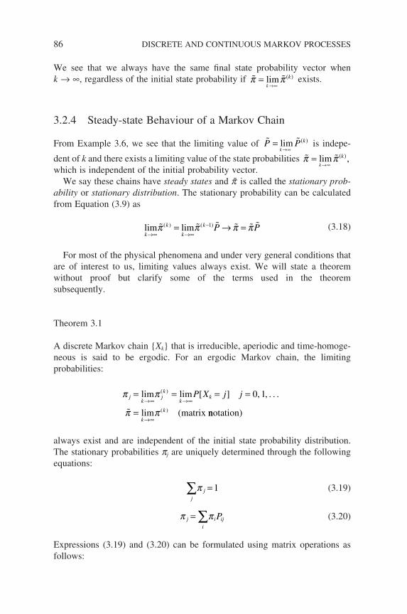
86 DISCRETE AND CONTINUOUS MARKOV PROCESSES
We see that we always have the same fi nal state probability vector when k → ∞, regardless of the initial state probability if π π= ( )
→∞lim k
k exists.
3.2.4 Steady-state Behaviour of a Markov Chain
From Example 3.6, we see that the limiting value of P P k
k= ( )
→∞lim is indepe-
dent of k and there exists a limiting value of the state probabilities π π= ( )→∞
lim ,k
kwhich is independent of the initial probability vector.
We say these chains have steady states and p is called the stationary prob-ability or stationary distribution. The stationary probability can be calculated from Equation (3.9) as
lim limk
k
k
k P P→∞ →∞
−= → = π π π π( ) ( )1 (3.18)
For most of the physical phenomena and under very general conditions that are of interest to us, limiting values always exist. We will state a theorem without proof but clarify some of the terms used in the theorem subsequently.
Theorem 3.1
A discrete Markov chain Xk that is irreducible, aperiodic and time-homoge-neous is said to be ergodic. For an ergodic Markov chain, the limiting probabilities:
π π
π π
jk
jk
kk
k
k
P X j j= = = =
=→∞ →∞
→∞
lim lim , , . . .
lim matrix
( )
( )
[ ]
(
0 1
nnotation)
always exist and are independent of the initial state probability distribution. The stationary probabilities pj are uniquely determined through the following equations:
j
j∑ =π 1 (3.19)
π πji
i ijP=∑ (3.20)
Expressions (3.19) and (3.20) can be formulated using matrix operations as follows:
p · e = 1
p = p · P
where e is a 1 × n row vector with all entries equal to one.To solve these two matrix equations, we fi rst defi ne a n × n matrix U with
all entries equal to one, then the fi rst equation can be rewritten as p · U = e. Students should note that these two matrices, U or e, have the summation property. Any matrix, say A = [aij], multiplied by U or e will give rise to a matrix in which every entry in a row is the same and is the sum of the corre-sponding row in A. For example:
a a
a a
a a a a
a a a a11 12
21 22
11 12 11 12
21 22 21 22
1 1
1 1
=
+ ++ +
Adding the two equations together, we have
π ( )P U I e+ − = (3.21)
We will postpone our discussion of some terms, for example, aperiodic and irreducible, used in the theorem to the next section and instead look at how we could use this theorem to calculate the steady-state probabilities of a Markov chain.
Example 3.7
Continuing with the lift example, the transition probabilities are given by
P pij= =
( )
/ /
/ /
/ /
0 1 2 1 2
3 4 0 1 4
3 4 1 4 0
and steady state probabilities p = [p0, p1, p2]. Using Equation (3.18) and expanding it, we have
π π π π
π π π π
π π π π
0 0 1 2
1 0 1 2
2 0 1 2
03
4
3
41
20
1
41
2
1
40
= + +
= + +
= + +
DISCRETE-TIME MARKOV CHAINS 87
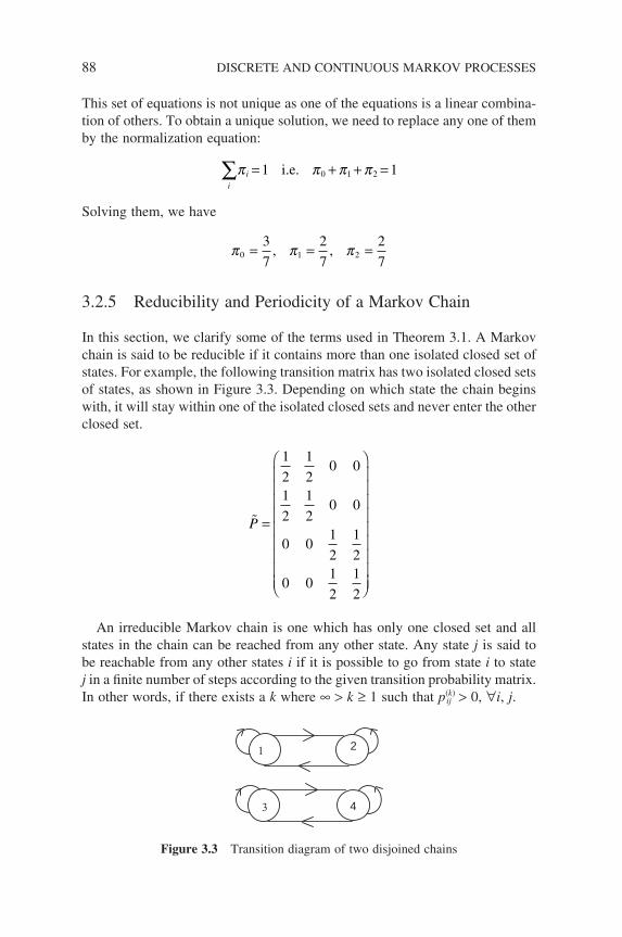
88 DISCRETE AND CONTINUOUS MARKOV PROCESSES
This set of equations is not unique as one of the equations is a linear combina-tion of others. To obtain a unique solution, we need to replace any one of them by the normalization equation:
ii∑ = + + =π π π π1 10 1 2i.e.
Solving them, we have
π π π0 1 23
7
2
7
2
7= = =, ,
3.2.5 Reducibility and Periodicity of a Markov Chain
In this section, we clarify some of the terms used in Theorem 3.1. A Markov chain is said to be reducible if it contains more than one isolated closed set of states. For example, the following transition matrix has two isolated closed sets of states, as shown in Figure 3.3. Depending on which state the chain begins with, it will stay within one of the isolated closed sets and never enter the other closed set.
P =
1
2
1
20 0
1
2
1
20 0
0 01
2
1
2
0 01
2
1
2
An irreducible Markov chain is one which has only one closed set and all states in the chain can be reached from any other state. Any state j is said to be reachable from any other states i if it is possible to go from state i to state j in a fi nite number of steps according to the given transition probability matrix. In other words, if there exists a k where ∞ > k ≥ 1 such that p(k)
ij > 0, ∀i, j.
3 4
21
Figure 3.3 Transition diagram of two disjoined chains

A Markov chain is said to be periodic with period t if it only returns to a particular state (say i) after nt(n = 1, 2, . . .) steps. Otherwise, it is aperiodic. In an irreducible Markov chain, all states are either all aperiodic or all periodic with the same period.
Example 3.8
The closed set of states in a probability transition matrix can be diffi cult to recognize. The following probability transition matrix represents the transitions shown in Figure 3.3, except now nodes 1 and 3 form a closed set and 2 and 4 another (Figure 3.4).
P =
1
20
1
20
01
20
1
21
20
1
20
01
20
1
2
In fact, students can verify that the above given transition-rate matrix can be reduced to
P =
1
2
1
20 0
1
2
1
20 0
0 01
2
1
2
0 01
2
1
2
through some appropriate row and column interchanges.
2 4
31
Figure 3.4 Transition diagram of two disjoined chains
DISCRETE-TIME MARKOV CHAINS 89
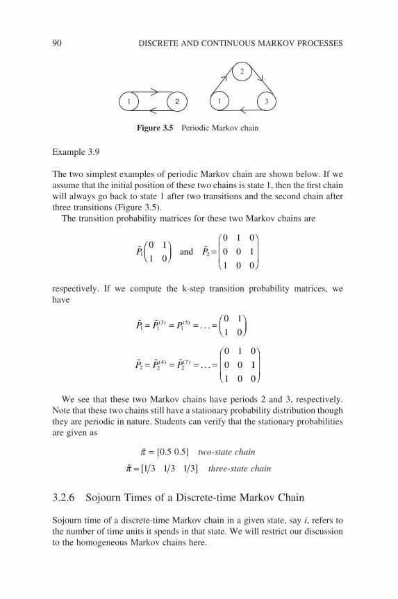
90 DISCRETE AND CONTINUOUS MARKOV PROCESSES
Example 3.9
The two simplest examples of periodic Markov chain are shown below. If we assume that the initial position of these two chains is state 1, then the fi rst chain will always go back to state 1 after two transitions and the second chain after three transitions (Figure 3.5).
The transition probability matrices for these two Markov chains are
P P1 2
0 1
1 0
0 1 0
0 0 1
1 0 0
=
and
respectively. If we compute the k-step transition probability matrices, we have
P P P
P P P
1 13
15
2 24
27
0 1
1 0
0 1 0
0 0
= = = =
= = = =
( ) ( )
( ) ( )
. . .
. . . 11
1 0 0
We see that these two Markov chains have periods 2 and 3, respectively. Note that these two chains still have a stationary probability distribution though they are periodic in nature. Students can verify that the stationary probabilities are given as
p = [0.5 0.5] two-state chain
π = [ ]1 3 1 3 1 3 three-state chain
3.2.6 Sojourn Times of a Discrete-time Markov Chain
Sojourn time of a discrete-time Markov chain in a given state, say i, refers to the number of time units it spends in that state. We will restrict our discussion to the homogeneous Markov chains here.
2
21 31
Figure 3.5 Periodic Markov chain
Assuming the Markov chain has just entered state i, the probability of it
staying in this state at the next time step is given by p pij iji j
= −≠∑1 . If it stays
in this state, again the probability of it staying in that state at the next time step is also pii. Hence, we see that the time a Markov chain stays in a state i, sojourn time Ri, is a geometrically distributed random variable with pmf:
P R k p p ki ii iik[ ] ( )= = − ∀ =−1 1 2 31, , , , . . . (3.22)
And the expected sojourn time is given by
E Rp
iii
[ ] =−1
1
The previous result of the sojourn time is in line with the memoryless prop-erty of a Markov chain. The geometric distribution is the only discrete pro-bability distribution that possesses such a memoryless property. Exponential distribution is the continuous version that also possesses such a property and we will show later that the sojourn times of a continuous-time Markov chain is exponentially distributed.
3.3 CONTINUOUS-TIME MARKOV CHAINS
Having discussed the discrete-time Markov chain, we are now ready to look at its continuous-time counterpart. Conceptually, there is no difference between these two classes of Markov chain; the past history of the chain is still being summarized in its present state and its future development can be inferred from there. In fact, we can think of the continuous-time Markov chain as being the limiting case of the discrete type.
However, there is a difference in mathematical formulation. In a continuous Markov chain, since transitions can take place at any instant of a time contin-uum, it is necessary now to specify how long a process has stayed in a particular state before a transition take place.
In some literature, the term ‘Markov process’ is also used to refer to a con-tinuous-time Markov chain. We use that term occasionally in subsequent chapters.
3.3.1 Defi nition of Continuous-time Markov Chains
The defi nition of a continuous-time Markov chain parallels that of a discrete-time Markov chain conceptually. It is a stochastic process X(t) in which the future probabilistic development of the process depends only on its present
CONTINUOUS-TIME MARKOV CHAINS 91
92 DISCRETE AND CONTINUOUS MARKOV PROCESSES
state and not on its past history. Mathematically, the process should satisfy the following conditional probability relationships for t1 < t2 < . . . < tk:
P X t j X t i X t t X t i P X t j X tk k k k[ ( ) | ( ) ( ) ( ) ] [ ( ) | (+ += = = = = =1 1 1 2 2 1, , . . . kk ki) ]=(3.23)
From the early discussion, we know that in the treatment of continuous-time Markov chains we need to specify a transition scheme by which the system goes from one state to another. The transition probability alone is not suffi cient to completely characterize the process. Instead of dwelling on its formal theo-retical basics which can be quite involved, we will take the following defi nition as the point of departure for our subsequent discussions and develop the neces-sary probability distribution. And again, we will focus our attention on the homogeneous case.
Defi nition 3.1
For a continuous Markov chain which is currently in state i, the probability that the chain will leave state i and go to state j(j ≠ i) in the next infi nitesimal amount of time ∆t, no matter how long the chain has been in state i, is
pij(t, t + ∆t) = qij∆t
where qij is the instantaneous transition rate of leaving state i for state j. In general, qij is a function of t. To simply the discussion, we assume that qij is independent of time; in other words, we are dealing with a homogeneous Markov chain. The total instantaneous transition rate at which the chain leaves
state i is, therefore, j i
ijq≠∑ .
3.3.2 Sojourn Times of a Continuous-time Markov Chains
Analogous to the discrete-time Markov chain, the sojourn times of a continu-ous-time Markov chain is the time the chain spends in a particular state. From the earlier discussion of Markov chains, we know that the future probabilistic development of a chain is only related to the past history through its current position. Thus, the sojourn times of a Markov chain must be ‘memoryless’ and are exponentially distributed, as exponential distribution is the only continuous probability distribution that exhibits such a memoryless property.
We shall demonstrate that the sojourn times of a continuous-time Markov chain are indeed exponentially distributed using the above defi nition. We assume the chain has just entered state i, and will remain in that during an interval [0, t].
Let ti be the random variable that denotes the time spent in state i. If we divide the time t into k equal intervals of ∆t, such that k∆t = t, then for the sojourn time ti to be greater than t, there should not be any transition in any of these ∆t intervals. From the above defi nition, we know that the probability of not having a transition in a time interval ∆t is
1−
≠
∑j i
ijq t∆
Therefore, the probability that the sojourn is greater than t
P t q t
qt
k
ik
j iij
k
kj i
ij
k
[ ]τ > = −
= −
=
→∞ ≠
→∞ ≠
∑
∑
lim
lim
1
1
∆
ee q ti−
(3.24)
where q qij i
ij= −≠∑ . Hence, the sojourn time between transitions is given by
P t P t ei iq ti[ ] [ ]τ τ≤ = − > = − −1 1 (3.25)
which is an exponential distribution.
3.3.3 State Probability Distribution
We will now turn our attention to the probability of fi nding the chain in a par-ticular state – state probability. As usual, we defi ne pj(t) = P[X(t) = j] and consider the probability change in an infi nitesimal amount of time ∆t:
π π πji j
i ij jk j
jkt t t q t t q t( ) ( ) ( )+ = + −
≠ ≠∑ ∑∆ ∆ ∆1 (3.26)
The fi rst term on the right is the probability that the chain is in state i at time t and makes a transition to state j in ∆t. The second term is the probability that the chain is in state j and does not make a transition to any other states in ∆t. Rearranging terms, dividing Equation (3.20) by ∆t and taking limits, we have
d
dtt q qj
i ji ij j
k jjkπ π π( ) = −
≠ ≠∑ ∑ (3.27)
CONTINUOUS-TIME MARKOV CHAINS 93
94 DISCRETE AND CONTINUOUS MARKOV PROCESSES
If we defi ne q qjjk j
ik= −≠∑ then the above expression can be re-written as
d
dtt t qj
ii ijπ π( ) ( )=∑ (3.28)
Let us defi ne the following three matrices:
π π π( ) ( ( ) ( )t t t= 1 2, , . . .) (3.29)
d
dtt
d
dtt
d
dttπ π π( ) ( ) ( )=
)1 2, , . . . (3.30)
Q q
q q q
q q q
q q
ij
jj
jj
nj n
nj
= =
−
−
−
≠
≠
≠
∑∑
∑
( )
11 12 13
212
2 23
1
(3.31)
We can then re-write Equation (3.27) or (3.28) in matrix form as
d
dtt t Q π π( ) ( )= (3.32)
The matrix Q is known as the infi nitesimal generator or transition-rate matrix as its elements are the instantaneous rates of leaving a state for another state. Recall from the section on ‘Eigenvalues, Eigenvectors and Spectral Representation’ in Chapter 1, one of the general solutions for the above matrix equation is given by
π t e IQ t
kQt
k k
k
( ) = = +( )
=
∞
∑ !1
Similar to the discrete-time Markov chains, the limiting value of the stateprobability π π=
→∞limt
t( ) exists for an irreducible homogeneous continuous-
time Markov chain and is independent of the initial state of the chain. That
implies that d
dttπ ( ) = 0 for these limiting values. Setting the differential of the
state probabilities to zero and taking limit, we have
0 = πQ (3.33)
where p = (p1, p2, . . .) and Q is the transition-rates matrix defi ned in Equation (3.31).
We can see the distinct similarity in structure if we compare this equation with that for a discrete-time Markov chain, i.e. p = p P. These two equations uniquely describe the ‘motion’ of a Markov chain and are called stationary equations. Their solutions are known as the stationary distributions.
3.3.4 Comparison of Transition-rate and Transition-probability Matrices
Comparing the transition rate matrix (3.31) defi ned in Section 3.3.3 with the transition probability matrix (3.7) of Section 3.2.2, we see some similarities as well as distinctions between them.
First of all, each of these two matrices completely characterizes a Markov chain, i.e. Q for a continuous Markov chain and P for the discrete counterpart. All the transient and steady-state probabilities of the corresponding chain can in principle be calculated from them in conjunction with the initial probability vector.
The main distinction between them lies in the fact that all entries in Q are transition rates whereas that of P are probabilities. To obtain probabilities in Q, each entry needs to be multiplied by ∆t, i.e. qij∆t.
Secondly, each row of the Q matrix sums to zero instead of one, as in the case of P matrix. The instantaneous transition rate of going back to itself is not
defi ned in the continuous case. It is taken to be q qjjk j
jk= −≠∑ just to place it
in the similar form as the discrete case. In general, we do not show self-loops on a state transition diagram as they are simply the negative sum of all rates leaving those states. On the contrary, self-loops on a state transition diagram for a discrete-time Markov chain indicate the probabilities of staying in those states and are usually shown on the diagram. Note that P and Q are related in the following expression:
d
dtP t P t Q Q t P t ( ) ( ) ( ) ( )= =
It is not surprising to see the similarity in form between the above expression and that governing the state probabilities because it can be shown that the fol-lowing limits always exist and are independent of the initial state of the chain for an irreducible homogeneous Markov chain:
limt
ij jp t→∞
=( ) π
and limt
j jt→∞
=π π( )
CONTINUOUS-TIME MARKOV CHAINS 95
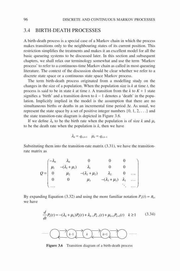
96 DISCRETE AND CONTINUOUS MARKOV PROCESSES
3.4 BIRTH-DEATH PROCESSES
A birth-death process is a special case of a Markov chain in which the process makes transitions only to the neighbouring states of its current position. This restriction simplifi es the treatments and makes it an excellent model for all the basic queueing systems to be discussed later. In this section and subsequent chapters, we shall relax our terminology somewhat and use the term ‘Markov process’ to refer to a continuous-time Markov chain as called in most queueing literature. The context of the discussion should be clear whether we refer to a discrete state space or a continuous state space Markov process.
The term birth-death process originated from a modelling study on the changes in the size of a population. When the population size is k at time t, the process is said to be in state k at time t. A transition from the k to K + 1 state signifi es a ‘birth’ and a transition down to k − 1 denotes a ‘death’ in the popu-lation. Implicitly implied in the model is the assumption that there are no simultaneous births or deaths in an incremental time period ∆t. As usual, we represent the state space by a set of positive integer numbers 0, 1, 2, . . . and the state transition-rate diagram is depicted in Figure 3.6.
If we defi ne lk to be the birth rate when the population is of size k and mk to be the death rate when the population is k, then we have
lk = qk,k+1 mk = qk,k−1
Substituting them into the transition-rate matrix (3.31), we have the transition-rate matrix as
Q =
−− +
− +− +
λ λµ λ µ λ
µ λ µ λµ λ µ λ
0 0
1 1 1 1
2 2 2 2
3 3 3 3
0 0 0
0 0
0 0
0 0
( )
( )
( )
. . .
. .
..
. . .
. . .
By expanding Equation (3.32) and using the more familiar notation Pk(t) = pk, we have
d
dtP t P t P t P t kk k k k k k k k( ) ( ) ( ) ( ) ( )= − + + + ≥− − + +λ µ λ µ1 1 1 1 1 (3.34)
k k+1k–1
Figure 3.6 Transition diagram of a birth-death process
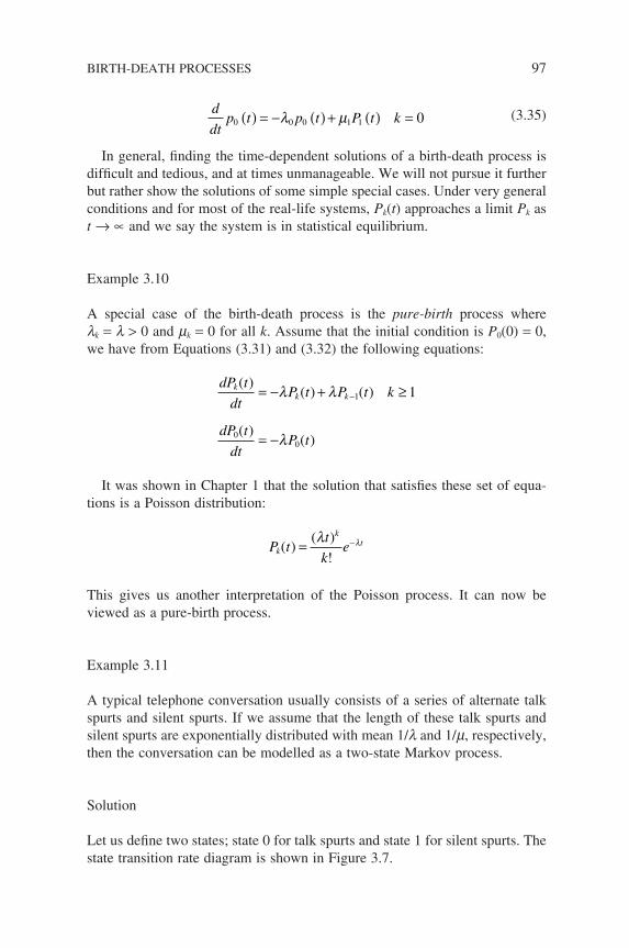
d
dtp t p t P t k0 0 0 1 1 0( ) = − ( ) + ( ) =λ µ
(3.35)
In general, fi nding the time-dependent solutions of a birth-death process is diffi cult and tedious, and at times unmanageable. We will not pursue it further but rather show the solutions of some simple special cases. Under very general conditions and for most of the real-life systems, Pk(t) approaches a limit Pk as t → ∝ and we say the system is in statistical equilibrium.
Example 3.10
A special case of the birth-death process is the pure-birth process where lk = l > 0 and mk = 0 for all k. Assume that the initial condition is P0(0) = 0, we have from Equations (3.31) and (3.32) the following equations:
dP t
dtP t P t k
dP t
dtP t
kk k
( )( ) ( )
( )( )
= − + ≥
= −
−λ λ
λ
1
00
1
It was shown in Chapter 1 that the solution that satisfi es these set of equa-tions is a Poisson distribution:
P tt
kek
kt( )
( )
!= −λ λ
This gives us another interpretation of the Poisson process. It can now be viewed as a pure-birth process.
Example 3.11
A typical telephone conversation usually consists of a series of alternate talk spurts and silent spurts. If we assume that the length of these talk spurts and silent spurts are exponentially distributed with mean 1/l and 1/m, respectively, then the conversation can be modelled as a two-state Markov process.
Solution
Let us defi ne two states; state 0 for talk spurts and state 1 for silent spurts. The state transition rate diagram is shown in Figure 3.7.
BIRTH-DEATH PROCESSES 97
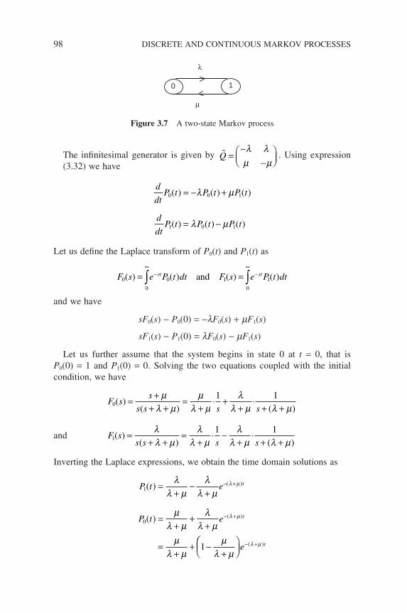
98 DISCRETE AND CONTINUOUS MARKOV PROCESSES
The infi nitesimal generator is given by Q =−
−
λ λµ µ
. Using expression(3.32) we have
d
dtP t P t P t
d
dtP t P t P t
0 0 1
1 0 1
( ) ( ) ( )
( ) ( ) ( )
= − +
= −
λ µ
λ µ
Let us defi ne the Laplace transform of P0(t) and P1(t) as
F s e P t dt F s e P t dtst st0
0
0 1
0
1( ) ( ) ( ) ( )= =∞
−∞
−∫ ∫and
and we have
sF0(s) − P0(0) = −lF0(s) + mF1(s)
sF1(s) − P1(0) = lF0(s) − mF1(s)
Let us further assume that the system begins in state 0 at t = 0, that is P0(0) = 1 and P1(0) = 0. Solving the two equations coupled with the initial condition, we have
F ss
s s s s0
1 1( )
( ) ( )= +
+ +=
+⋅ +
+⋅
+ +µ
λ µµ
λ µλ
λ µ λ µ
and F ss s s s
11 1
( )( ) ( )
=+ +
=+
⋅ −+
⋅+ +
λλ µ
λλ µ
λλ µ λ µ
Inverting the Laplace expressions, we obtain the time domain solutions as
P t e
P t e
t
t
1
0
1
( )
( )
)
( )
=+
−+
=+
++
=+
+ −+
−( +
− +
λλ µ
λλ µ
µλ µ
λλ µ
µλ µ
µλ µ
λ µ
λ µ
− +e t( )λ µ
0 1
λ
µ
Figure 3.7 A two-state Markov process
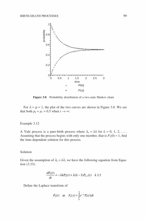
For l = m = 1, the plot of the two curves are shown in Figure 3.8. We see that both p0 = p1 = 0.5 when t → ∞:
Example 3.12
A Yule process is a pure-birth process where lk = kl for k = 0, 1, 2, . . . . Assuming that the process begins with only one member, that is P1(0) = 1, fi nd the time-dependent solution for this process.
Solution
Given the assumption of lk = kl, we have the following equation from Equa-tion (3.33):
dP t
dtkP t k P t kk
k k( )
( ) ( ) ( )= − + − ≥−λ λ 1 11
Defi ne the Laplace transform of
P t F s e P t dtk kst
k( ) ( ) ( )as =∞
−∫0
1
prob
abili
ty
0.8
0.6
0.4
0.2
00 0.5 1 1.5 2 2.5 3
timeP0(t)
P1(t)
Figure 3.8 Probability distribution of a two-state Markov chain
BIRTH-DEATH PROCESSES 99
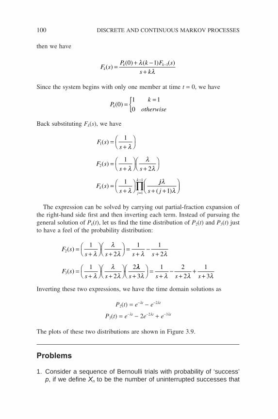
100 DISCRETE AND CONTINUOUS MARKOV PROCESSES
then we have
F sP k F s
s kk
k k( )( ) ( ) ( )= + −
+−0 1 1λ
λ
Since the system begins with only one member at time t = 0, we have
Pk
otherwisek( )0
1 1
0=
=Back substituting Fk(s), we have
F ss
F ss s
F ss
kj
k
1
2
1
1
1
1
2
1
( )
( )
( )
=+
=+
+
=+
=
−
∏
λ
λλ
λ
λjj
s j
λλ+ +
( )1
The expression can be solved by carrying out partial-fraction expansion of the right-hand side fi rst and then inverting each term. Instead of pursuing the general solution of Pk(t), let us fi nd the time distribution of P2(t) and P3(t) just to have a feel of the probability distribution:
F ss s s s
F ss s
2
3
1
2
1 1
2
1
2
2
( )
( )
=+
+
=
+−
+
=+
+
λλ
λ λ λ
λλ
λλλλ λ λ λs s s s+
=
+−
++
+3
1 2
2
1
3
Inverting these two expressions, we have the time domain solutions as
P2(t) = e−lt − e−2lt
P3(t) = e−lt − 2e−2lt + e−3lt
The plots of these two distributions are shown in Figure 3.9.
Problems
1. Consider a sequence of Bernoulli trials with probability of ‘success’ p, if we defi ne Xn to be the number of uninterrupted successes that
have been completed at n trial; that is if the fi rst 6 outcomes are ‘S’, ‘F’, ‘S’,’S’, ‘S’, ‘F’; then X1 = 1, X2 = 0, X3 = 1, X4 = 2, X5 = 3, X6 = 0.
(i) argue that Xn is a Markov chain(ii) draw the state transition diagram and write down the one-step
transition matrix.
2. By considering a distributed system that consists of three processors (A, B and C), a job which has been processed in processor A has a probability p of being redirected to processor B and probability (1 − p) to processor C for further processing. However, a job at processor B is always redirected back to process A after completion of its pro-cessing, whereas at processor C a job is redirected back to proces-sor B q fraction of the time and (1 − q) fraction of the time it stays in processor C.
(i) Draw the state transition diagram for this multi-processor system.
(ii) Find the probability that a job X is in processor B after 2 routings assuming that the job X was initially with processor A.
(iii) Find the steady-state probabilities.(iv) Find value of p and q for which the steady state probabilities are
all equal.
0.25
prob
abili
ty
0.2
0.15
0.1
0.05
00 1 2 3 4 5 6
time axis
P2(t)
P3(t)
Figure 3.9 Probability distribution of a Yule process
BIRTH-DEATH PROCESSES 101
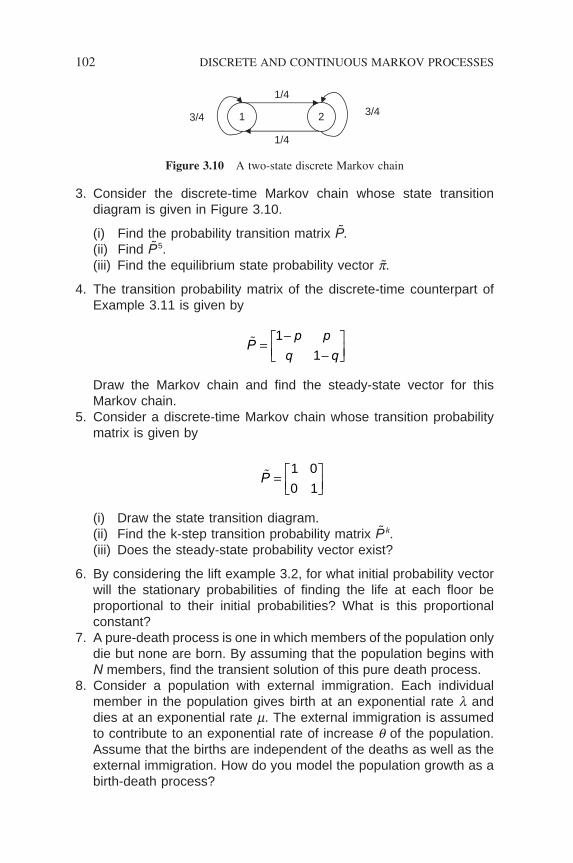
102 DISCRETE AND CONTINUOUS MARKOV PROCESSES
3. Consider the discrete-time Markov chain whose state transition diagram is given in Figure 3.10.
(i) Find the probability transition matrix P.(ii) Find P5.(iii) Find the equilibrium state probability vector p.
4. The transition probability matrix of the discrete-time counterpart of Example 3.11 is given by
Pp p
q q=
−−
1
1
Draw the Markov chain and fi nd the steady-state vector for this Markov chain.
5. Consider a discrete-time Markov chain whose transition probability matrix is given by
P =
1 0
0 1
(i) Draw the state transition diagram.(ii) Find the k-step transition probability matrix P k.(iii) Does the steady-state probability vector exist?
6. By considering the lift example 3.2, for what initial probability vector will the stationary probabilities of fi nding the life at each fl oor be proportional to their initial probabilities? What is this proportional constant?
7. A pure-death process is one in which members of the population only die but none are born. By assuming that the population begins with N members, fi nd the transient solution of this pure death process.
8. Consider a population with external immigration. Each individual member in the population gives birth at an exponential rate l and dies at an exponential rate m. The external immigration is assumed to contribute to an exponential rate of increase q of the population. Assume that the births are independent of the deaths as well as the external immigration. How do you model the population growth as a birth-death process?
1 2
1/4
3/4
1/4
3/4
Figure 3.10 A two-state discrete Markov chain
4Single-Queue Markovian Systems
In Chapter 3 we showed that it was easier to determine N(t), the number of customers in the system, if it could be modelled as a Markov process. Here, we shall demonstrate the general approach employed in obtaining these per-formance measures of a Markovian queueing system using the Markov chain theory. We fi rst model the number of customers present in a queueing system as a birth-death process and then compute the equilibrium state probability Pk using balance equations. Once Pk is found, we can then calculate N using the expression:
N kPk
k= ∑
and then proceed to evaluate other parameters that are of interest by using Little’s theorem.
A Markovian queueing system is one characterized by a Poisson arrival process and exponentially distributed service times. In this chapter we will examine only this group of queueing systems or those that can be adapted as such. These queueing models are useful in applications to data communications and networking. The emphasis here is on the techniques of computing these performance measures rather than to comprehensively cover all queueing systems. Students are referred to (Kleinrock 1975) which gives an elegant analysis for a collection of queueing systems.
We assume all the queueing systems we deal with throughout this book are ergodic and we shall focus our attention on the queueing results in the steady
Queueing Modelling Fundamentals Second Edition Ng Chee-Hock and Soong Boon-Hee© 2008 John Wiley & Sons, Ltd
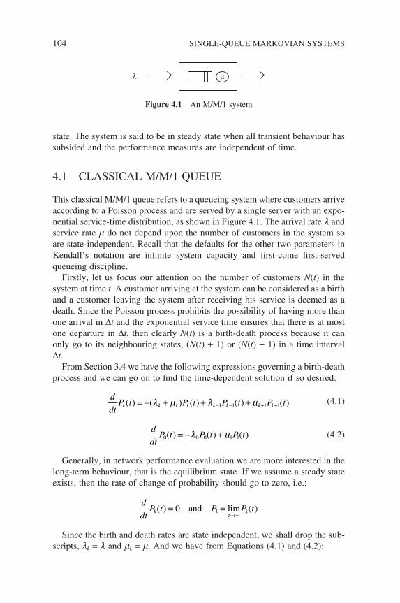
104 SINGLE-QUEUE MARKOVIAN SYSTEMS
state. The system is said to be in steady state when all transient behaviour has subsided and the performance measures are independent of time.
4.1 CLASSICAL M/M/1 QUEUE
This classical M/M/1 queue refers to a queueing system where customers arrive according to a Poisson process and are served by a single server with an expo-nential service-time distribution, as shown in Figure 4.1. The arrival rate l and service rate m do not depend upon the number of customers in the system so are state-independent. Recall that the defaults for the other two parameters in Kendall’s notation are infi nite system capacity and fi rst-come fi rst-served queueing discipline.
Firstly, let us focus our attention on the number of customers N(t) in the system at time t. A customer arriving at the system can be considered as a birth and a customer leaving the system after receiving his service is deemed as a death. Since the Poisson process prohibits the possibility of having more than one arrival in ∆t and the exponential service time ensures that there is at most one departure in ∆t, then clearly N(t) is a birth-death process because it can only go to its neighbouring states, (N(t) + 1) or (N(t) − 1) in a time interval ∆t.
From Section 3.4 we have the following expressions governing a birth-death process and we can go on to fi nd the time-dependent solution if so desired:
d
dtP t P t P t P tk k k k k k k k( ) ( ) ( ) ( ) ( )= − + + +− − + +λ µ λ µ1 1 1 1
(4.1)
d
dtP t P t P t0 0 0 1 1( ) ( ) ( )= − +λ µ (4.2)
Generally, in network performance evaluation we are more interested in the long-term behaviour, that is the equilibrium state. If we assume a steady state exists, then the rate of change of probability should go to zero, i.e.:
d
dtP t P P tk k
tk( ) ( )= =
→∞0 and lim
Since the birth and death rates are state independent, we shall drop the sub-scripts, lk = l and mk = m. And we have from Equations (4.1) and (4.2):
µλ
Figure 4.1 An M/M/1 system
( )λ µ λ µ+ = +− +P P Pk k k1 1 (4.3)
µ λP P1 0= (4.4)
Equation (4.3) is a recursive expression and we shall solve it using z-trans-form. Multiplying the whole equation by zk and summing from one to infi nity, we have
kk
k
kk
k
kk
kP z P z P z=
∞
=
∞
−=
∞
+∑ ∑ ∑+ = +1 1
11
1( )λ µ λ µ
( )[ ( ) ] ( ) [ ( ) ]λ µ λ µ+ − = + − −P z P zP z
zP z P z P0 1 0
Coupled with the boundary conditions of Equation (4.4), P P1 0= λµ
, we have
( ) ( ) [ ( ) ] ( )
( )( )
( )
λ µ µ µ λ
µλ λ µ µ
+ − = − +
=−
− + +=
P z Pz
P z P zP z
P zP z
z z
0 0
0
2
1 PP z
z z
P
z
Pz
0
0
0
1
1
1
1
1
µλ µ
λµ
ρρ λ µ
( )
( )( )
/
−− −
=−
=−
=where
(4.5)
To evaluate P0, we use the normalization condition k
kp=
∞
∑ =0
1 , which is
equivalent to P(z)z=1 = 1. Setting z = 1 and P(z) = 1, we have
P0 1 1= − = −λ
µρ
(4.6)
Hence we arrive at
P zz
( ) = −−
1
1
ρρ
(4.7)
and
CLASSICAL M/M/1 QUEUE 105
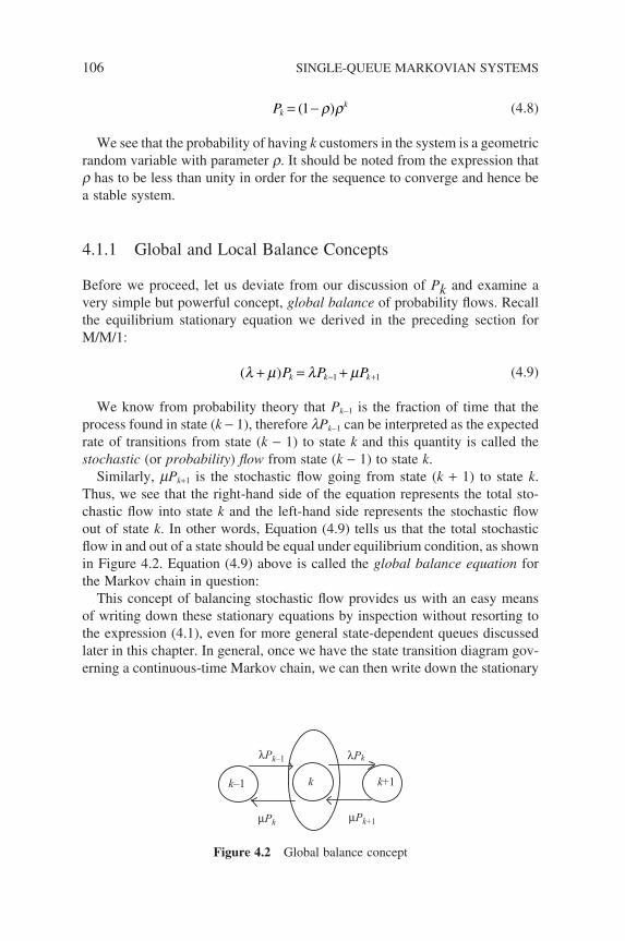
106 SINGLE-QUEUE MARKOVIAN SYSTEMS
Pkk= −( )1 ρ ρ (4.8)
We see that the probability of having k customers in the system is a geometric random variable with parameter r. It should be noted from the expression that r has to be less than unity in order for the sequence to converge and hence be a stable system.
4.1.1 Global and Local Balance Concepts
Before we proceed, let us deviate from our discussion of Pk and examine a very simple but powerful concept, global balance of probability fl ows. Recall the equilibrium stationary equation we derived in the preceding section for M/M/1:
( )λ µ λ µ+ = +− +P P Pk k k1 1 (4.9)
We know from probability theory that Pk−1 is the fraction of time that the process found in state (k − 1), therefore lPk−1 can be interpreted as the expected rate of transitions from state (k − 1) to state k and this quantity is called the stochastic (or probability) fl ow from state (k − 1) to state k.
Similarly, mPk+1 is the stochastic fl ow going from state (k + 1) to state k. Thus, we see that the right-hand side of the equation represents the total sto-chastic fl ow into state k and the left-hand side represents the stochastic fl ow out of state k. In other words, Equation (4.9) tells us that the total stochastic fl ow in and out of a state should be equal under equilibrium condition, as shown in Figure 4.2. Equation (4.9) above is called the global balance equation for the Markov chain in question:
This concept of balancing stochastic fl ow provides us with an easy means of writing down these stationary equations by inspection without resorting to the expression (4.1), even for more general state-dependent queues discussed later in this chapter. In general, once we have the state transition diagram gov-erning a continuous-time Markov chain, we can then write down the stationary
k–1 k k+1
λPk
µPk µPk+1
λPk–1
Figure 4.2 Global balance concept
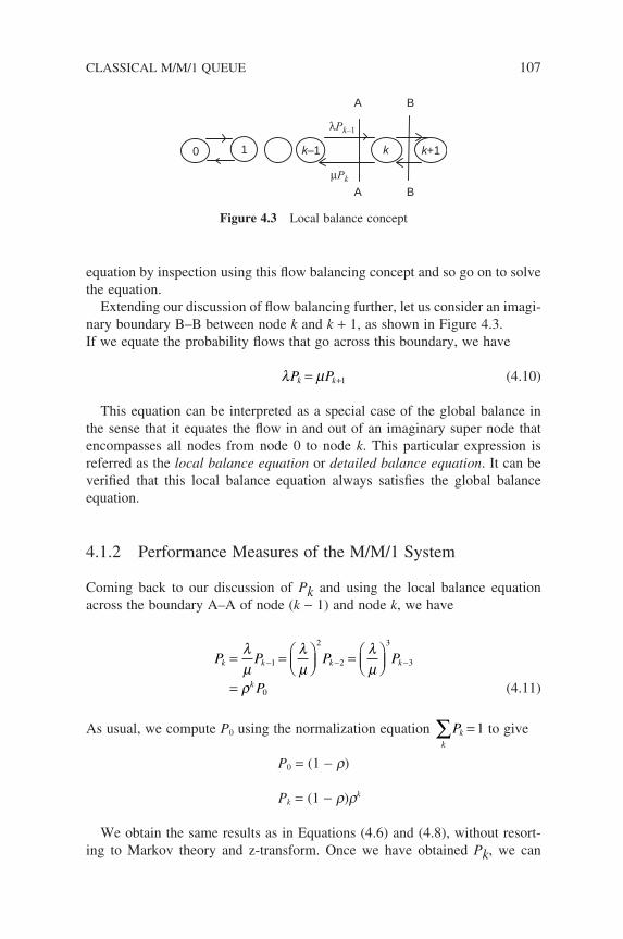
equation by inspection using this fl ow balancing concept and so go on to solve the equation.
Extending our discussion of fl ow balancing further, let us consider an imagi-nary boundary B–B between node k and k + 1, as shown in Figure 4.3.If we equate the probability fl ows that go across this boundary, we have
λ µP Pk k= +1 (4.10)
This equation can be interpreted as a special case of the global balance in the sense that it equates the fl ow in and out of an imaginary super node that encompasses all nodes from node 0 to node k. This particular expression is referred as the local balance equation or detailed balance equation. It can be verifi ed that this local balance equation always satisfi es the global balance equation.
4.1.2 Performance Measures of the M/M/1 System
Coming back to our discussion of Pk and using the local balance equation across the boundary A–A of node (k − 1) and node k, we have
P P P P
P
k k k k
k
= =
=
=
− − −λµ
λµ
λµ
ρ
1
2
2
3
3
0
(4.11)
As usual, we compute P0 using the normalization equation k
kP∑ = 1 to give
P0 = (1 − r)
Pk = (1 − r)rk
We obtain the same results as in Equations (4.6) and (4.8), without resort-ing to Markov theory and z-transform. Once we have obtained Pk, we can
µPk
λPk–1
0 1 k k+1k–1
A
A
B
B
Figure 4.3 Local balance concept
CLASSICAL M/M/1 QUEUE 107
108 SINGLE-QUEUE MARKOVIAN SYSTEMS
proceed to fi nd other performance measures using Little’s theorem. Students should note that this local balance concept offers a simpler expression for computing Pk and this should be the preferred approach as far as possible:
(i) The probability of having n or more customers in the system is given by
P N n Pk n
k
k n
k
k
k
k
nk
[ ]
( )
( )
(
≥ =
= −
= − −
=
=
∞
=
∞
=
∞
=
−
∑
∑
∑ ∑
1
10 0
1
ρ ρ
ρ ρ ρ
111
1
1
1−
−−
−−
=
ρρ
ρρ
ρ
)n
n
(4.12)
(ii) The average number of customers N in the system in steady state is then given by
N kP k
k
kk
k
k
k
k
= = −( )
= −
=−
=−
=
∞
=
∞
=
∞−
∑ ∑
∑0 0
0
1
1
1
1
ρ ρ
ρ ρ ρ
ρρ
λµ λ
( )
(4.13)
and the variance of N can be calculated as
σ ρρN
kkk N p2
0
221
= − =−=
∞
∑( )( )
(4.14)
Figure 4.4 shows the average number of customers as a function of utiliza-tion r. As the utilization (load) approaches the full capacity of the system (r = 1), the number of customers grows rapidly without limit and the system becomes unstable. Again, we see that for the system to be stable, the condition is r < 1.
This is a signifi cant result for a single isolated queueing system and is the basis of the ‘two-third’ design rule. In practice, we usually design a shared
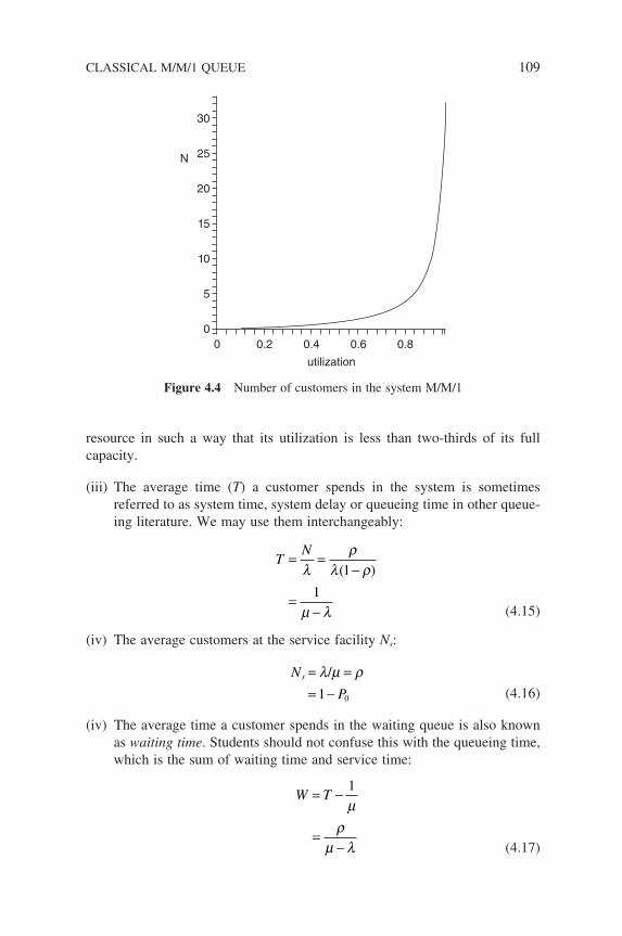
resource in such a way that its utilization is less than two-thirds of its full capacity.
(iii) The average time (T) a customer spends in the system is sometimes referred to as system time, system delay or queueing time in other queue-ing literature. We may use them interchangeably:
T
N= =−
=−
λρ
λ ρ
µ λ
( )1
1
(4.15)
(iv) The average customers at the service facility Ns:
N
Ps = == −
λ µ ρ/
1 0
(4.16)
(iv) The average time a customer spends in the waiting queue is also known as waiting time. Students should not confuse this with the queueing time, which is the sum of waiting time and service time:
W T= −
=−
1
µρ
µ λ
(4.17)
30
25N
20
15
10
5
00 0.2 0.4 0.6
utilization
0.8
Figure 4.4 Number of customers in the system M/M/1
CLASSICAL M/M/1 QUEUE 109
110 SINGLE-QUEUE MARKOVIAN SYSTEMS
(vi) The average number of customers in the waiting queue:
N Wq =
=−
λ
ρρ
2
1
(4.18)
Alternatively, Nq can be found by the following argument:
N Nq = − ρ
(4.19)
=−
− −−
=−
ρρ
ρ ρρ
ρρ
1
1
1
1
2
( )
It should be noted that these steady-state performance measures are derived without any assumption about the queueing discipline and they hold for all queueing disciplines which are work conserving. Simply put, work conserving means that the server is always busy as long as there are customers in the system.
4.2 PASTA – POISSON ARRIVALS SEE TIME AVERAGES
Before we proceed, let us revisit the Poisson arrival process and examine a very useful and important concept called Poisson Arrivals See Time Averages (PASTA). This concept will be used below to obtain the distribution functions of system and waiting times.
Basically, this property states that for a stable queueing system with Poisson arrivals, the probability distribution as seen by an arriving customer is the same as the time-averaged (equilibrium or ergodic) state probability. In other words, the state N(t) = k of the queueing system seen by an arrival has the same probability distribution as the state seen by an external random observer. That is
A t P tk k( ) ( )= (4.20)
Here Ak(t) is the probability of fi nding k customers in the system by an arriving customer and Pk(t) is the steady-state probability of the system in state k. By defi nition:
A t P N t k An arrival at time t
P N t k An arrival at time tk( ) [ ( ) | ]
[ ( )
≡ =
== , ]]
[ ]
[ | ( ) ] [ ( ) ]
P An arrival at time t
P An arrival at time t N t k P N t k=
= ⋅ =PP An arrival at time t[ ]
However, we know that the event of an arrival at time t is independent of the process N(t) = k because of the memoryless property of Poisson process. That is
P[An arrival at time t N(t) = k] = P[An arrival at time t]
Therefore, substituting in the preceding expression, we obtain
A t P N t k P tk k( ) [ ( ) ] ( )= = = (4.21)
In the limit of t → ∞, we have
A Pk k= (4.22)
4.3 M/M/1 SYSTEM TIME (DELAY) DISTRIBUTION
In previous sections, we obtained several performance measures of an M/M/1 queue, so we are now in a position to predict the long-range averages of this queue. However, we are still unable to say anything about the probability that a customer will spend up to 3 minutes in the system or answer any questions on that aspect. To address them, we need to examine the actual probability distribution of both the system time and waiting time. Let us defi ne the system-time density function as
f td
dtP T tT( ) [ ]= <
Students should note that the probability distributions (or density functions) of system time or waiting time depend very much on the actual service disci-pline used, although the steady state performance measures are independent of the service discipline.
We assume here that FCFS discipline is used and focus our attention on the arrival of customer i. The system time of this customer will be the sum of his/her service time and the service times of those customers (say k of them) ahead
M/M/1 SYSTEM TIME (DELAY) DISTRIBUTION 111
112 SINGLE-QUEUE MARKOVIAN SYSTEMS
of him/her if the system is not empty when he/she arrives. Otherwise, his/her system time will be just his/her own service time. That is
Tx x x x k
x ki k
i
=+ + + + ≥
= 1 2 1
0
. . . (4.23)
Owing to the memoryless property of exponential service times, the remaining service time needed to fi nish serving the customer currently in service is still exponentially distributed. Hence the density function of T is simply the convolution of all the service times which are all exponentially distributed.
Using Laplace transform, the conditional system-time density function is
L f t ks
kT
k
[ ( | )] =+
=
+µµ
1
0 1 2, , , . . . (4.24)
Earlier we obtained Pk = (1 − r)rk, hence the Laplace transform of the unconditional probability density function can be obtained using the total prob-ability theorem:
L f t
s
s
Tk
kk[ ( )] ( )
( )
=+
−
= −+ −
=
∞ +
∑0
1
1µ
µρ ρ
µ λµ λ
(4.25)
Inverting the above expression, we have
f t e tTt( ) ( ) ( )= − >− −µ λ µ λ , 0 (4.26)
and the cumulative distribution function FT(t) is
F t P T t eTt( ) [ ] ( )= ≤ = − − −1 µ λ (4.27)
At this juncture, it is important to point out that the above expression was actually derived with respect to an arriving customer. However, owing to the PASTA property of a Poisson arrival process, these probability distributions are the same as the long-range time averages or, in other words, distributions seen by a random observer.
Once the density function of system time is found, the density function of waiting time fw(t) can be found by considering:
T w x= + (4.28)
Taking Laplace transform, we have
µ λµ λ
µµ
µ ρµ λ
ρ λ
−+ −
=+
=+ −+ −
= − +
sL f s
s
L f ss
s
w
w
( )[ ( )]
( ( )]( )( )
( )
( )(
1
111−
+ −ρ
µ λ)
( )s
(4.29)
Inverting
f t t ewt( ) ( ) ( ) ( ) ( )= − + − − −1 1ρ δ λ ρ µ λ (4.30)
where d(t) is the impulse function or Dirac delta function.Integrating we have the waiting time cumulative distribution function
Fw(t):
F t ewt( ) ( )= − − −1 ρ µ λ (4.31)
Example 4.1
At a neighhourhood polyclinic, patients arrive according to a Poisson process with an average inter-arrival time of 18 minutes. These patients are given a queue number upon arrival and will be seen, by the only doctor manning the clinic, according to their queue number. The length of a typical consultation session is found from historical data to be exponentially distributed with a mean of 7 minutes:
(i) What is the probability that a patient has to wait to see the doctor?(ii) What is the average number of patients waiting to see the doctor?(iii) What is the probability that there are more than 5 patients in the clinic,
including the one in consultation with the doctor?(iv) What is the probability that a patient would have to wait more than 10
minutes for this consultation?(v) The polyclinic will employ an additional doctor if the average waiting time
of a patient is at least 7 minutes before seeing the doctor. By how much must the arrival rate increase in order to justify the additional doctor?
Solution
Assuming the clinic is suffi ciently large to accommodate a large number of patients, the situation can be modelled as an M/M/1 queue. Given the following parameters:
M/M/1 SYSTEM TIME (DELAY) DISTRIBUTION 113
114 SINGLE-QUEUE MARKOVIAN SYSTEMS
l = 1/18 person/min and m = 1/7 person/min
We have r = 7/18:
(i) P[patient has to wait] = r = 1 − P0 = 7/18(ii) The waiting-queue length Nq = r2 /(1 − r) = 49/198(iii) P[N ≥ 5] = r5 = 0.0089(iv) Since P[waitingtime ≤ 10] = 1 − re−m(1−r)t,
P e[ ] ./ /queueing time > = =− −( )×107
180 1621 7 1 7 18 10
(v) Let the new arrival rate be l′
then 7
17
71
14′
− ′≥ ⇒ ′ =λ
λλ person/min person/min.
Example 4.2
Variable-length data packets arrive at a communication node according to a Poisson process with an average rate of 10 packets per second. The single outgoing communications link is operating at a transmission rate of 64 kbits per second. As a fi rst-cut approximation, the packet length can be assumed to be exponentially distributed with an average length of 480 characters in 8-bit ASCII format. Calculate the principal performance mea-sures of this communication link assuming that it has a very large input buffer. What is the probability that 6 or more packets are waiting to be transmitted?
Solution
Again the situation can be modelled as an M/M/1 with the communication link being the server.
The average service time:
x = × =480 8
640000 06. s
and the arrival rate
l = 10 packets/second
thus
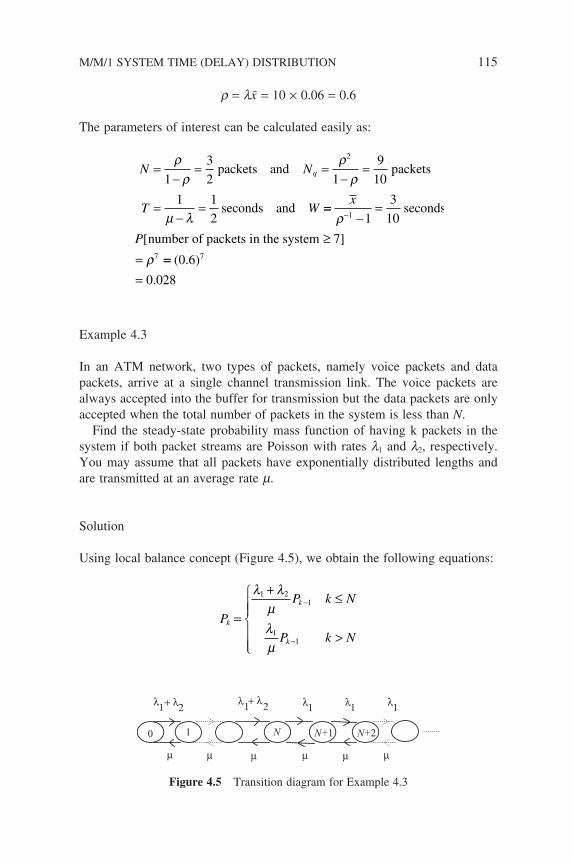
r = lx = 10 × 0.06 = 0.6
The parameters of interest can be calculated easily as:
N N
T W
q=−
= =−
=
=−
=
ρρ
ρρ
µ λ
1
3
2 1
9
10
1 1
2
2
packets and packets
seconds and ==−
=
≥=
−
x
P
ρ
ρ
1
7
1
3
10
7
seconds
number of packets in the system[ ]
===
( . )
.
0 6
0 028
7
Example 4.3
In an ATM network, two types of packets, namely voice packets and data packets, arrive at a single channel transmission link. The voice packets are always accepted into the buffer for transmission but the data packets are only accepted when the total number of packets in the system is less than N.
Find the steady-state probability mass function of having k packets in the system if both packet streams are Poisson with rates l1 and l2, respectively. You may assume that all packets have exponentially distributed lengths and are transmitted at an average rate m.
Solution
Using local balance concept (Figure 4.5), we obtain the following equations:
P
P k N
P k Nk
k
k
=
+≤
>
−
−
λ λµλµ
1 21
11
0 1 N+1 N+2
λ1+ λ2
N
λ1+ λ2 λ1 λ1
µ µ µ µ µ µ
λ1
Figure 4.5 Transition diagram for Example 4.3
M/M/1 SYSTEM TIME (DELAY) DISTRIBUTION 115
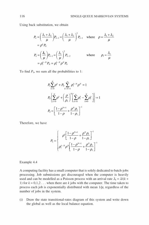
116 SINGLE-QUEUE MARKOVIAN SYSTEMS
Using back substitution, we obtain
P P P
P
P
k k k
k
k
=+
=
+
=
=+
=
− −λ λ
µλ λ
µρ
ρ λ λµ
1 21
1 22
1
0
1 2where
λλµ
λµ
ρ ρ ρ
ρ λµ
11
12
2
1 1 0
11
=
= =
=− −
− −
P P
P P
k k
k NN
k N N
where
To fi nd P0, we sum all the probabilities to 1:
P P
P
k
Nk
k N
k N N
k
Nk
N
k
k
k
00
01
1
00 1 0
1
1= = +
∞−
= =
∞
∑ ∑
∑ ∑
+ =
+
−
ρ ρ ρ
ρ ρρ
ρ==
+ −
∑
=
=−
−+
−
01
0
11
1
1
1
1
1 1
Nk
N N
P
ρ
ρρ
ρ ρρ
Therefore, we have
Pk
kN N
k N NN N
=
−−
+−
−−
+−
+ −
−+
ρ ρρ
ρ ρρ
ρ ρ ρρ
ρ ρρ
1
1 1
1
1 1
11
1
1
1
11
1
−1
Example 4.4
A computing facility has a small computer that is solely dedicated to batch-jobs processing. Job submissions get discouraged when the computer is heavily used and can be modelled as a Poisson process with an arrival rate lk = l/(k + 1) for k = 0,1,2 . . . when there are k jobs with the computer. The time taken to process each job is exponentially distributed with mean 1/m, regardless of the number of jobs in the system.
(i) Draw the state transitional-rates diagram of this system and write down the global as well as the local balance equation.
(ii) Find the steady-state probability Pk that there are k jobs with the computer and then fi nd the average number of jobs.
(iii) Find the average time taken by a job from submission to completion.
Solution
(i) With reference to node k (Figure 4.6), we have
Global: Pk
Pk
Pk k kµ λ λ µ++
) = +− +
11 1
With reference to the boundary between nodes k − 1 and k, we have
Local:λ µk
P Pk k= −1
(ii) From the local balance equation, we obtain
Pk k
Pk
Pk k
k
=−
= =−ρ ρ ρ λ µ
2
2 01( ) !
/where
Summing all the probabilities to 1, we have
k
k
kP P e
=
∞−∑ = ⇒ =
00 01
ρ ρ
!
Therefore
Pk
ek
k
= −ρ ρ
!
Since Pk is Poisson distributed, the average number of jobs N = r.
0 1 k–1 k k+1
λ λ/2 λ/k λ/k+1
µ µµ µ µ µ
Figure 4.6 Transition diagram for Example 4.4
M/M/1 SYSTEM TIME (DELAY) DISTRIBUTION 117
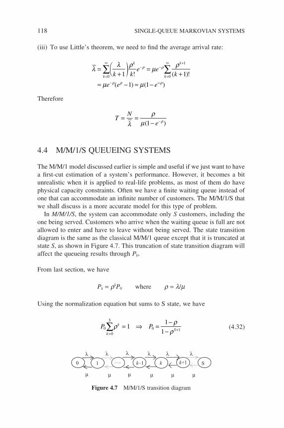
118 SINGLE-QUEUE MARKOVIAN SYSTEMS
(iii) To use Little’s theorem, we need to fi nd the average arrival rate:
λ λ ρ µ ρ
µ µ
ρ ρ
ρ ρ
=+
) =
+= − = −
=
∞− −
=
∞ +
−
∑ ∑k
k
k
k
k ke e
k
e e e
0 0
1
1 1
1 1
! ( )!
( ) ( −−ρ)
Therefore
TN
e= =
− −λρ
µ ρ( )1
4.4 M/M/1/S QUEUEING SYSTEMS
The M/M/1 model discussed earlier is simple and useful if we just want to have a fi rst-cut estimation of a system’s performance. However, it becomes a bit unrealistic when it is applied to real-life problems, as most of them do have physical capacity constraints. Often we have a fi nite waiting queue instead of one that can accommodate an infi nite number of customers. The M/M/1/S that we shall discuss is a more accurate model for this type of problem.
In M/M/1/S, the system can accommodate only S customers, including the one being served. Customers who arrive when the waiting queue is full are not allowed to enter and have to leave without being served. The state transition diagram is the same as the classical M/M/1 queue except that it is truncated at state S, as shown in Figure 4.7. This truncation of state transition diagram will affect the queueing results through P0.
From last section, we have
Pk = rkP0 where r = l/m
Using the normalization equation but sums to S state, we have
P Pk
Sk
S00
0 11
1
1=+∑ = ⇒ =
−−
ρ ρρ
(4.32)
0 1 k–1 k k+1 S
λ
µ
λ λ λλ λ
µ µµ µ µ
Figure 4.7 M/M/1/S transition diagram
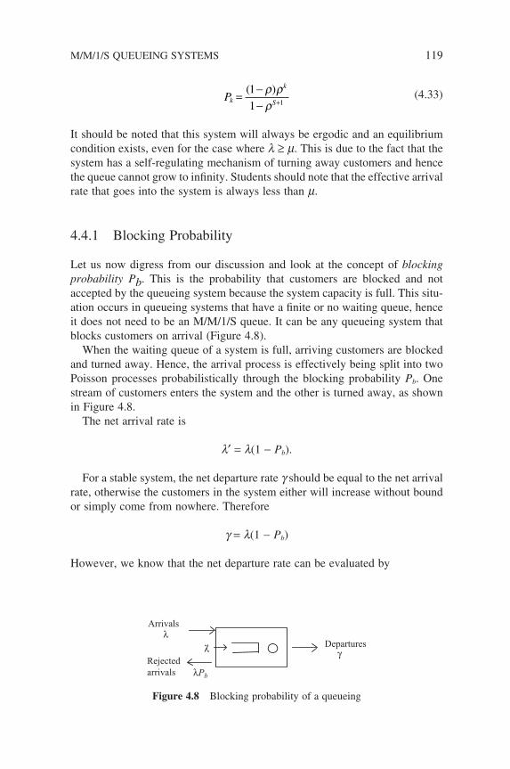
Pk
k
S= −
− +
( )1
1 1
ρ ρρ
(4.33)
It should be noted that this system will always be ergodic and an equilibrium condition exists, even for the case where l ≥ m. This is due to the fact that the system has a self-regulating mechanism of turning away customers and hence the queue cannot grow to infi nity. Students should note that the effective arrival rate that goes into the system is always less than m.
4.4.1 Blocking Probability
Let us now digress from our discussion and look at the concept of blocking probability Pb. This is the probability that customers are blocked and not accepted by the queueing system because the system capacity is full. This situ-ation occurs in queueing systems that have a fi nite or no waiting queue, hence it does not need to be an M/M/1/S queue. It can be any queueing system that blocks customers on arrival (Figure 4.8).
When the waiting queue of a system is full, arriving customers are blocked and turned away. Hence, the arrival process is effectively being split into two Poisson processes probabilistically through the blocking probability Pb. One stream of customers enters the system and the other is turned away, as shown in Figure 4.8.
The net arrival rate is
l′ = l(1 − Pb).
For a stable system, the net departure rate g should be equal to the net arrival rate, otherwise the customers in the system either will increase without bound or simply come from nowhere. Therefore
g = l(1 − Pb)
However, we know that the net departure rate can be evaluated by
Departuresλ
λPb
Arrivals
Rejectedarrivals
γλ'
Figure 4.8 Blocking probability of a queueing
M/M/1/S QUEUEING SYSTEMS 119
120 SINGLE-QUEUE MARKOVIAN SYSTEMS
γ µ µ= = −=
∑k
S
kP P1
01( ) (4.34)
Equating both expressions, we obtain
λ µ
ρρ
( ) ( )1 1
1
0
0
− = −
=+ −
P P
PP
b
b
(4.35)
The expression is derived for a queueing system with constant arrival and service rates; if they are state-dependent, then the corresponding ensemble averages should be used.
4.4.2 Performance Measures of M/M/1/S Systems
Continuing with our early discussion, the various performance measures can then be computed once Pk is found:
(i) The saturation probabilityBy defi nition, the saturation probability is the probability when the system is full; that is there are S customers in the system. We say the system is saturated and we have
PS
S
S= −
− +
( )1
1 1
ρ ρρ
However, substituting P0 of M/M/1/S into expression (4.35), we have
PP
b
S
S= + − = −
− +0
1
1 1
1
ρρ
ρ ρρ
( ) (4.36)
That is just the expression for Ps. This result is intuitively correct as it indicates that the blocking probability is the probability when the system is saturated. Owing to this blocking probability, the system now has a built-in self-regulatory mechanism and we see for the fi rst time that it is still stable even when arrival rate is great than the service rate.
For r = 1, the expression for the blocking probability has to be evalu-ated using L’Hopital’s rule and we have
PS
b =+1
1
(ii) The average number of customers in the system is given by
N kP
k
k
k
S
k
k
S
Sk
Sk
s
=
= −−
= −−
=
=+
+=
∑
∑
∑
0
11
11
1
1
1
1
ρρ
ρ
ρρ
ρ ρkk
Sk
sk
S
S
d
d
S
−
+=
+
+
= −−
=−
− +−
=−
−
∑
1
11
1
1
1
1
1
1
1
1
ρρ
ρρ
ρ
ρρ
ρρ
ρρ
( )
ρρρ1
1−
+( )S PS
(4.37)
Again, for r = 1, the expression has to be evaluated by L’Hopital’s rule and we have
NS=2
(4.38)
(iii) The average number of customers at the service facility:
N P k E N k P k E N N
PP
s s s
S
= = = + > >= −= −
[ ] [ | ] [ ] [ | ]
( )
0 0 0 01
10
ρ
(4.39)
(iv) The average number of customers in the waiting queue:
N N NS
Pq s S= − =−
− +−
ρρ
ρ ρρ
2
1 1
( ) (4.40)
(v) The average time spent in the system and in the waiting queue.Since customers are blocked when there are S customers in the system, the effective arrival rate of customers admitted into the system is
′ = −λ λ( )1 Ps (4.41)
and the T and W can be computed as
TN S S
S=
′=
−−
−
+
+λ µ λρ
λ µρ1 1
1 (4.42)
M/M/1/S QUEUEING SYSTEMS 121
122 SINGLE-QUEUE MARKOVIAN SYSTEMS
WN Sq
S
S=
′=
−−
−
+
+λρ
µ λρ
λ µρ
1
1 (4.43)
Example 4.5
Variable-length packets arrive at a network switching node at an average rate of 125 packets per second. If the packet lengths are exponentially distributed with a mean of 88 bits and the single outgoing link is operating at 19.2 kb/s, what is the probability of buffer overfl ow if the buffer is only big enough to hold 11 packets? On average, how many packets are there in the buffer? How big should the buffer be in terms of number of packets to keep packet loss below 10−6?
Solution
Given l = 125 pkts/s m−1 = 88/19200 = 4.6 × 10⁻³ s r = lm−1 = 0.573
P
N
S
S
S
q
=−−
=−
−= ×
+
−
( ) ( . )( . )
( . )
.
1
1
1 0 573 0 573
1 0 573
5 35 10
1
12
13
4
ρ ρρ
==−
−+−
=
=−
−≤+
−
ρρ
ρρ
2
16
1 10 75
1 0 573 0 573
1 0 57310
SP
P
d
d
S
S
.
( . )( . )
( . )
The above equation is best solved by trial and error. By trying various numbers, we have
S = 23 Pd = 1.2 × 10⁻⁶
S = 24 Pd = 6.7 × 10⁻⁷
Therefore, a total of 24 buffers is required to keep packet loss below 1 packet per million.
Example 4.6
Let us compare the performance of a statistical multiplexer with that of a fre-quency-division multiplexer. Assume that each multiplexer has 4 inputs of 5
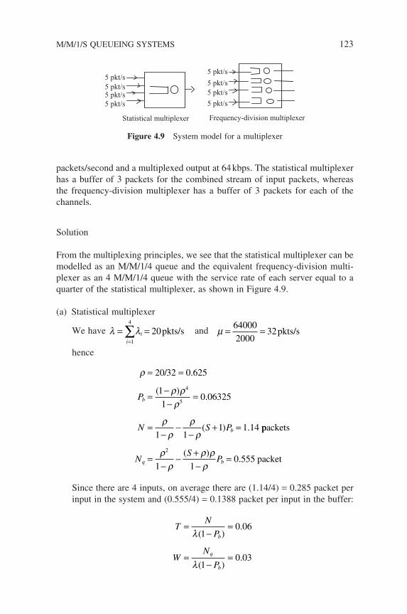
packets/second and a multiplexed output at 64 kbps. The statistical multiplexer has a buffer of 3 packets for the combined stream of input packets, whereas the frequency-division multiplexer has a buffer of 3 packets for each of the channels.
Solution
From the multiplexing principles, we see that the statistical multiplexer can be modelled as an M/M/1/4 queue and the equivalent frequency-division multi-plexer as an 4 M/M/1/4 queue with the service rate of each server equal to a quarter of the statistical multiplexer, as shown in Figure 4.9.
(a) Statistical multiplexer
We have λ λ= ==∑i
i1
4
20pkts/s and µ = =64000
200032pkts/s
hence
ρ
ρ ρρ
ρρ
ρρ
= =
=−−
=
=−
−−
+ =
20 32 0 625
1
10 06325
1 11 1 14
4
5
/ .
( ).
( ) .
P
N S P
b
b ppackets
packetNS
Pq b=−
−+−
=ρ
ρρ ρρ
2
1 10 555
( ).
Since there are 4 inputs, on average there are (1.14/4) = 0.285 packet per input in the system and (0.555/4) = 0.1388 packet per input in the buffer:
TN
P
WN
P
b
q
b
=−
=
=−
=
λ
λ
( ).
( ).
10 06
10 03
Statistical multiplexer Frequency-division multiplexer
5 pkt/s
5 pkt/s5 pkt/s
5 pkt/s
5 pkt/s5 pkt/s5 pkt/s
5 pkt/s
Figure 4.9 System model for a multiplexer
M/M/1/S QUEUEING SYSTEMS 123
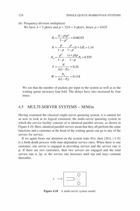
124 SINGLE-QUEUE MARKOVIAN SYSTEMS
(b) Frequency-division multiplexer We have l = 5 pkts/s and m = 32/4 = 8 pkts/s, hence r = 0.625
P
N S P
Ns
b
b
q
=−−
=
=−
−−
+ =
=−
−+
( ).
( ) .
(
1
10 06325
1 11 1 14
1
4
5
2
ρ ρρ
ρρ
ρρ
ρρ
ρ)).
( ).
( ).
ρρ
λ
λ
10 555
10 24
10 118
−=
=−
=
=−
=
P
TN
P
WN
P
b
b
q
b
We see that the number of packets per input in the system as well as in the waiting queue increases four-fold. The delays have also increased by four times.
4.5 MULTI-SERVER SYSTEMS – M/M/m
Having examined the classical single-server queueing system, it is natural for us now to look at its logical extension; the multi-server queueing system in which the service facility consists of m identical parallel servers, as shown in Figure 4.10. Here, identical parallel servers mean that they all perform the same functions and a customer at the head of the waiting queue can go to any of the servers for service.
If we again focus our attention on the system state N(t), then N(t), t ≥ 0 is a birth-death process with state-dependent service rates. When there is one customer, one server is engaged in providing service and the service rate is m. If there are two customers, then two servers are engaged and the total service rate is 2m, so the service rate increases until mm and stays constant thereafter.
λ
Figure 4.10 A multi-server system model
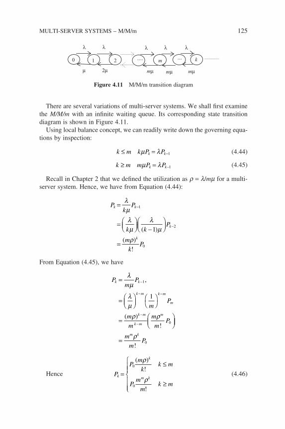
There are several variations of multi-server systems. We shall fi rst examine the M/M/m with an infi nite waiting queue. Its corresponding state transition diagram is shown in Figure 4.11.
Using local balance concept, we can readily write down the governing equa-tions by inspection:
k m k P Pk k≤ = −µ λ 1 (4.44)
k m m P Pk k≥ = −µ λ 1 (4.45)
Recall in Chapter 2 that we defi ned the utilization as r = l/mm for a multi-server system. Hence, we have from Equation (4.44):
Pk
P
k kP
m
kP
k k
k
k
=
=
−
=
−
−
λµλµ
λµ
ρ
1
2
0
1( )
( )
!
From Equation (4.45), we have
Pm
P
mP
m
m
m
mP
k k
k m k m
m
k m
k m
m
=
=
=
−
− −
−
−
λµ
λµ
ρ ρ
1
0
1
,
( )
!
=m
mP
m kρ!
0
Hence P
Pm
kk m
Pm
mk m
k
k
m k=
≤
≥
0
0
( )
!
!
ρ
ρ (4.46)
0 1 2 .... m ... k
λ λ
µ 2µ
λ λλ
mµ mµmµ
Figure 4.11 M/M/m transition diagram
MULTI-SERVER SYSTEMS – M/M/m 125
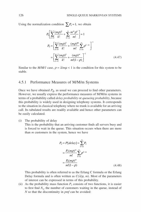
126 SINGLE-QUEUE MARKOVIAN SYSTEMS
Using the normalization condition ∑ =Pk 1, we obtain
Pm
k
m
m
Pm
k
m
k
m k
k m
m k
k
m k
00
1
00
1
1=
−
=
∞
=
−
∑ ∑
∑
+
=
= +
( )
! !
( )
!
( )
ρ ρ
ρ ρ mm
k m
k m
k
m k m
m
m
k
m
m
!
( )
!
( )
!( )
=
∞−
−
=
− −
∑
∑
= +−
ρ
ρ ρρ
1
0
1 1
1 (4.47)
Similar to the M/M/1 case, r = l/mm < 1 is the condition for this system to be stable.
4.5.1 Performance Measures of M/M/m Systems
Once we have obtained Pk, as usual we can proceed to fi nd other parameters. However, we usually express the performance measures of M/M/m systems in terms of a probability called delay probability or queueing probability, because this probability is widely used in designing telephony systems. It corresponds to the situation in classical telephony where no trunk is available for an arriving call. Its tabulated results are readily available and hence other parameters can be easily calculated.
(i) The probability of delay This is the probability that an arriving customer fi nds all servers busy and
is forced to wait in the queue. This situation occurs when there are more than m customers in the system, hence we have
P P delay P
P m
m
P m
m
dk m
k
om
k m
k m
m
= =
=
=−
=
∞
=
∞−
∑
∑
[ ]
( )
!
( )
!( )
ρ ρ
ρρ
0
1
(4.48)
This probability is often referred to as the Erlang C formula or the Erlang Delay formula and is often written as C(l/m, m). Most of the parameters of interest can be expressed in terms of this probability.
(ii) As the probability mass function Pk consists of two functions, it is easier to fi rst fi nd Nq, the number of customers waiting in the queue, instead of N so that the discontinuity in pmf can be avoided:
N kP Pm
mk
Pm
m
Pm
qk
m k
m
k
k
m
d
= =
=−
=−
=
=
∞
+=
∞
∑ ∑0
00
0 21
1
( )
!
( )
! ( )
ρ ρ
ρ ρρ
ρρ
λµµ λ−
Pd (4.49)
(iii) The time spent in the waiting queue:
WN
mPq
d= =−λ µ λ
1 (4.50)
(iv) The time spends in the queueing system:
T WP
md= + =−
+1 1
µ µ λ µ (4.51)
(v) The number of customers in the queueing system:
N T P md= =−
+λ ρρ
ρ1
(4.52)
4.5.2 Waiting Time Distribution of M/M/m
Parallel to the M/M/1 case, we will continue with the examination of the waiting time distribution in this section. Again, we are going to make use of the PASTA concept to derive the function. Let us focus our attention on an arriving customer i to the system. He/her may fi nd k customers waiting in the queue upon arrival, meaning there are n = (k + m) customers in the system. He/she may also fi nd no customers waiting in the queue, meaning the total number of customers is n ≤ m − 1.
We denote the waiting time of this customers i as w, and its density function as fw(t) and cumulative probability function Fw(t); then we have
F t P w tP w t no waiting P w t k
w( ) [ ][ ] [ ]
= <= < + < ≥, , 0
(4.53)
Let us examine each individual term on the right-hand side of the expression. The fi rst term is simply the probability of having n ≤ m − 1 customers in the system, hence no waiting:
MULTI-SERVER SYSTEMS – M/M/m 127
128 SINGLE-QUEUE MARKOVIAN SYSTEMS
P w t no waiting P n m
P Pm
kn
m
nn
m k
[ ] [ ]
( )
!
< = ≤ −
= ==
−
=
−
∑ ∑
, 1
0
1
00
1 ρ (4.54)
But, we have from Equation (4.47):
Pm
k
m
mk
m k m
00
1 1
1= +
−
=
− −
∑ ( )
!
( )
!( )
ρ ρρ
Pm
k
P m
mk
m k m
00
101
1=
−
∑ = −−
( )
!
( )
!( )
ρ ρρ
Hence
P w t no waitingP m
m
m
[ ]( )
!( )< = −
−, 1
10 ρ
ρ (4.55)
The second term depicts the situation where customer i has to wait in the queue. His/her waiting time is simply the sum of the service time xj ( j = 1, . . . k) of those k customers in the queue as well as the service time x of those customers currently in service. That is
w = x + x1 + x2 + . . . + xk
The service times are all exponentially distributed with a rate mm, as there are m servers. Therefore the density function of w is simply the convolution of these service times, and in Laplace transform domain, the multiplication of them. Thus we have
L f t km
s mkw
k
( | ) =+
= ∞
+µµ
1
0 1, , , . . . ,
and
L f tm
s mP
m
s mPw
k
k
k mk
k
( ) =+
⋅ =
+
⋅
=
∞ +
+=
∞ +
∑ ∑0
1
0
1
0µ
µµ
µmm
m
Pm
m
m
s m
m
s m
Pm
mk m
m
k
kk
!
( )
!
(
ρ
ρ µµ
µµ
ρ
ρ
+
=
∞
=+
+
⋅
=
∑00
0))
!
( )
!
m
m
m
m
s m
s m
s m
Pm
m
m
s m
µµ
µµ λ
ρ µµ λ
+
++ −
=+ −
0
(4.56)
Inverting the Laplace transform, we have
f t Pm
mm ew
mm t( )
( )
!( ) ( )= ⋅ − −
0ρ µ µ λ (4.57)
Integrating the density function, we obtain
F t Pm
m
m
m gle
Pm
m
w
mm t
m
( )( )
!( )
( )
( ) !
( )= −−
⋅ −
=−
− −0
0
1
1
ρ µµ
ρρ
µ λ
⋅⋅ − − −( )( )1 e m tµ λ
(4.58)
Combining both Equations (4.55) and (4.58), we have
F tP m
m
P m
me
P m
w
m mm t( )
( )
!( )
( )
( ) !( )
(
( )= −−
+−
⋅ −
= −
− −11 1
1
1
0 0
0
ρρ
ρρ
µ λ
ρρρ
µ λ
µ λ
)
( ) !( )
( )
mm t
dm t
me
P e
1
1
−= −
− −
− −
(4.59)
where Pd is the delay (queueing) probability. We see the similarity of this expression with that of the M/M/1 case, except now the r is replaced with Pd and m with mm.
The time a customer spent in the system, system time or system delay, is simply his/her waiting time plus his/her own service time, i.e. T = w + x. Note that his/her service time is exponentially distributed with m instead of mm as the service rate of each individual server is m. It can then be shown that the cumulative probability function of system time FT(t) is given by
F t P eP
mm e eT d
t d m t t( ) ( )( )
( ) ( )( )= − +− −
− −− − − −11 1
1µρ
ρ µµ µ λ µ (4.60)
4.6 ERLANG’S LOSS QUEUEING SYSTEMS – M/M/m/m SYSTEMS
Similar to the single-server case, the assumption of infi nite waiting queue may not be appropriate in some applications. Instead of looking at the multi-server system with fi nite waiting queue, we shall examine the extreme case M/M/m/m system where there is no waiting queue. This particular model has been widely used in evaluating the performance of circuit-switched telephone systems. It corresponds to the classical case where all the trunks
ERLANG’S LOSS QUEUEING SYSTEMS – M/M/m/m SYSTEMS 129
130 SINGLE-QUEUE MARKOVIAN SYSTEMS
of a telephone system are occupied and connection cannot be set up for further calls.
Since there is no waiting queue, when a customer arrives at the system and fi nds all servers engaged, the customer will not enter the system and is consid-ered lost. The state transition diagram is the same as that of M/M/m except that it is truncated at state m.
Again using local balance concept, we have the following equation by inspection:
λ µ
ρ
P k P
P Pm
k
k k
k
k
− =
=
1
0( )
!
(4.61)
Solving for P0:
Pm
kk
m k
00
1
=
=
−
∑ ( )
!
ρ (4.62)
hence, we have
P
m k
m
k
k
k
k
m k=
=
∑( ) / !
( )!
ρρ
0
(4.63)
Again this system is stable even for r = l/mm ≥ 1 because of this self-regulating mechanism of turning away customers when the system is full.
4.6.1 Performance Measures of the M/M/m/m
(i) The probability that an arrival will be lost when all servers are busy:
P
m m
m k
Pb
m
k
mk
m= =
=∑( ) / !
( ) / !
ρ
ρ0
(4.64)
This probability is the blocking probability and is the same as the probability when the system is full. It is commonly referred to as the Erlang B formula or Erlang’s loss formula and is often written as B(l/m,m).
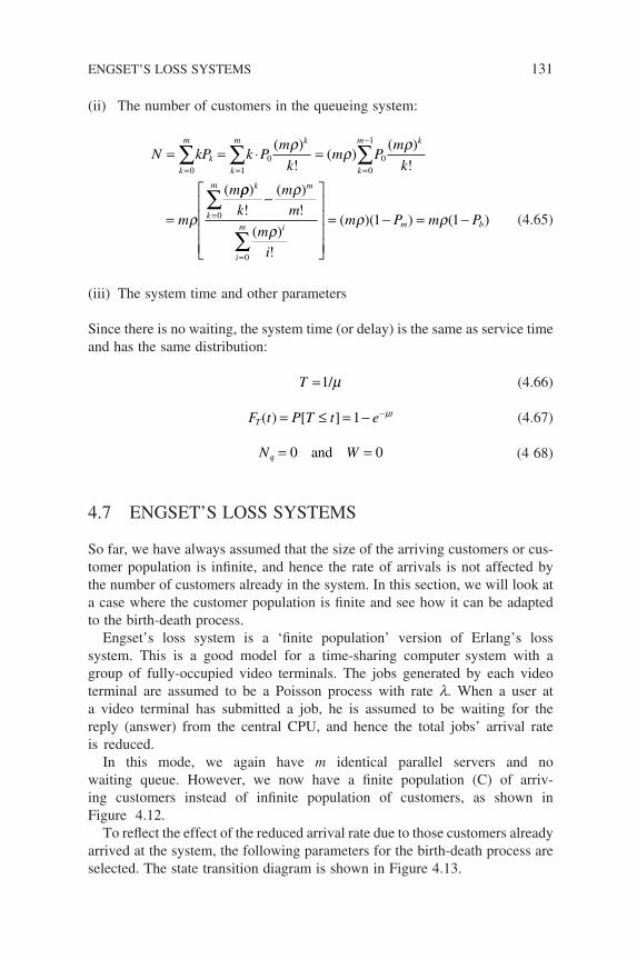
(ii) The number of customers in the queueing system:
N kP k Pm
km P
m
k
m
m
k
m
kk
m k
k
m k
k
m
= = ⋅ =
=
= = =
−
=
∑ ∑ ∑
∑0 1
00
1
0
0
( )
!( )
( )
!
(
ρ ρ ρ
ρ
ρρ ρ
ρρ ρ
)!
( )!
( )!
( )( ) ( )
k m
i
m i m b
k
m
m
m
i
m P m P
−
= − = −
=∑
0
1 1
(4.65)
(iii) The system time and other parameters
Since there is no waiting, the system time (or delay) is the same as service time and has the same distribution:
T =1/µ (4.66)
F t P T t eTt( ) [ ]= ≤ = − −1 µ (4.67)
N Wq = =0 0and (4 68)
4.7 ENGSET’S LOSS SYSTEMS
So far, we have always assumed that the size of the arriving customers or cus-tomer population is infi nite, and hence the rate of arrivals is not affected by the number of customers already in the system. In this section, we will look at a case where the customer population is fi nite and see how it can be adapted to the birth-death process.
Engset’s loss system is a ‘fi nite population’ version of Erlang’s loss system. This is a good model for a time-sharing computer system with a group of fully-occupied video terminals. The jobs generated by each video terminal are assumed to be a Poisson process with rate l. When a user at a video terminal has submitted a job, he is assumed to be waiting for the reply (answer) from the central CPU, and hence the total jobs’ arrival rate is reduced.
In this mode, we again have m identical parallel servers and no waiting queue. However, we now have a fi nite population (C) of arriv-ing customers instead of infi nite population of customers, as shown in Figure 4.12.
To refl ect the effect of the reduced arrival rate due to those customers already arrived at the system, the following parameters for the birth-death process are selected. The state transition diagram is shown in Figure 4.13.
ENGSET’S LOSS SYSTEMS 131
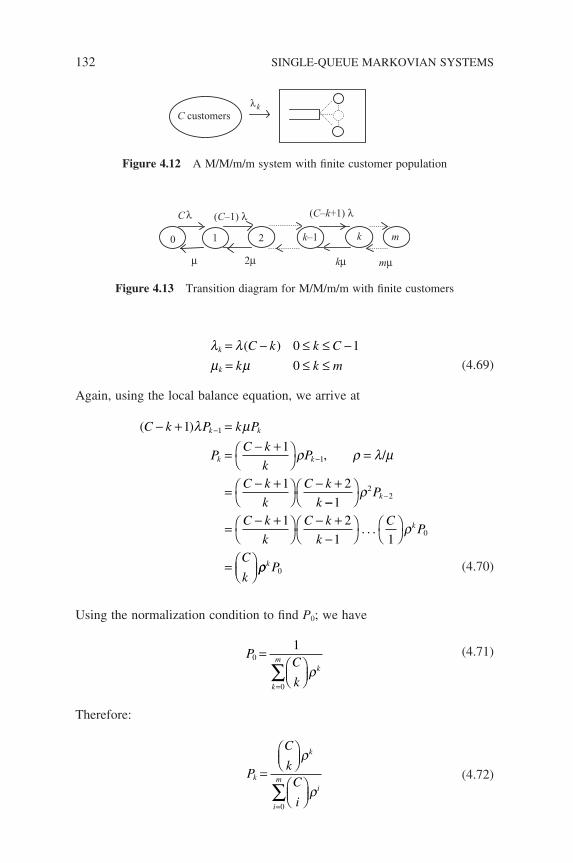
132 SINGLE-QUEUE MARKOVIAN SYSTEMS
λ λµ µ
k
k
C k k C
k k m
= − ≤ ≤ −= ≤ ≤
( ) 0 1
0
(4.69)
Again, using the local balance equation, we arrive at
( )
/
C k P k P
PC k
kP
C k
k
C k
k
k k
k k
− + =
=− +
=
=− +
− +
−
−
1
1
1 2
1
1
λ µ
ρ ρ λ µ,
−−
=− +
− +−
=
−1
1 2
1 1
22
0
ρ
ρ
P
C k
k
C k
k
CP
C
k
k
k. . .
ρρk P0
(4.70)
Using the normalization condition to fi nd P0; we have
P
C
kk
mk
0
0
1=
=
∑ ρ (4.71)
Therefore:
P
C
kC
i
k
k
i
mi
=
=
∑
ρ
ρ0
(4.72)
0 1 2 k m
λ
µ 2µ
k–1
C (C–1) λ (C–k+1) λ
mµkµ
Figure 4.13 Transition diagram for M/M/m/m with fi nite customers
λC customers
k
Figure 4.12 A M/M/m/m system with fi nite customer population
If the population size C of the arriving customers is the same as the number of servers in the system, i.e. C = m, then
P
m
km
i
m
kk
k
i
mi
k
m=
=
+=∑
ρ
ρ
ρ
ρ0
1( ) (4.73)
4.7.1 Performance Measures of M/M/m/m with Finite Customer Population
(i) The probability of blocking; that is the probability of having all m servers engaged:
P P
C
mC
k
b m
m
k
mk
= =
=
∑
ρ
ρ0
(4.74)
(ii) The number of customers in the queueing system.
Instead of the usual approach, it is easier in this case to compute N by fi rst calculating the average arrival rate l:
λ λ λ ρ
λ
= = −
=
=
−
=
−
=
−
∑ ∑
∑k
m
k kk
mk
k
m
P C k PC
k
C
C
k
0
1
0
1
0
0
1
( )
−
=
=
=
−
=∑
∑
∑
ρ
ρλ
ρ
ρ
k
k
mk
k
mk
k
mk
C
k
C
kC
k0
0
1
0
λλρ ρ
ρλC
C
k
C
mC
k
kC
kk
mk m
k
mk
k
m
=
=
=∑
∑
∑
−
−
0
0
0 −
= − − −=
∑
ρ ρ
ρ
λ λ
k m
k
mk
b b
mC
mC
k
C P N mP0
1( ) ( )
(4.75)
where N is the expected number of customers in the system and is given by the usual defi nition:
N P kC
kk
mk=
=
∑00
ρ (4.76)
ENGSET’S LOSS SYSTEMS 133
134 SINGLE-QUEUE MARKOVIAN SYSTEMS
But we know that
N T= = ×λ λµ1
therefore
N C P N mP
N C C m P
b b
b
= − − −
=+
−+
−
11
1 1
µλ λ
ρρ
ρρ
[ ( ) ( )]
( )
(4.77)
where
ρ λµ
=
If the population size C of the arriving customers is the same as the number of servers in the system, i.e. C = m, then
N m=+ρ
ρ1 (4.78)
(iii) The system time
T = 1
µ (4.79)
4.8 CONSIDERATIONS FOR APPLICATIONS OF QUEUEING MODELS
Those queueing models discussed so far are fairly elegant in analysis and yield simple closed-form results owing to the memoryless property of Poisson process and exponential service times. However, how valid are the assump-tions of Poisson arrival process and exponential service times in real-life applications?
From the past observation and studies, the Poisson arrival has been found to be fairly accurate in modelling the arrival of calls in a telephone network, and hence was extensively used in designing such networks. It is a fairly good model as long as the arriving customer population is large and there is no interdependency among them on arrival. It may not fully match the arrival
process of some other real-life problems, but so long as the discrepancy is small, it can be treated as the fi rst-cut approximation.
The exponential service time assumption appears to be less ideal than the Poisson assumption but still offers fairly good results as far as voice networks are concerned. However, it may be inadequate in modelling packets or mes-sages in data networks as the length of a packet is usually constrained by the physical implementation. The length could even be a constant, as in the case of ATM (Asynchronous Transfer Mode) networks. Nevertheless, the exponen-tial distribution can be deemed as the worst-case scenario and will give us the fi rst-cut estimation.
The M/M/1 queue and its variants can be used to study the performance measure of a switch with input buffer in a network. In fact, its multi-server counterparts have traditionally been employed in capacity planning of tele-phone networks. Since A K Erlang developed them in 1917, the M/M/m and M/M/m/m models have been extensively used to analyse the ‘lost-calls-cleared’ (or simply blocked-calls) and ‘lost-calls-delayed’ (queued-calls) telephone systems, respectively. A ‘queued-calls’ telephone system is one which puts any arriving call requests on hold when all the telephone trunks are engaged, whereas the ‘blocked-calls’ system rejects those arriving calls.
In a ‘blocked-calls’ voice network, the main performance criterion is to determine the probability of blocking given an offered load or the number of trunks (circuits) needed to provide certain level of blocking. The performance of a ‘queued-calls’ voice network is characterized by the Erlang C formula and its associated expressions.
Example 4.6
A trading company is installing a new 300-line PBX to replace its old exist-ing over-crowded one. The new PBX will have a group of two-way external circuits and the outgoing and incoming calls will be split equally among them.
It has been observed from past experience that each internal telephone usually generated (call or receive) 20 minutes of voice traffi c during a typical busy day. How many external circuits are required to ensure a blocking prob-ability of 0.02?
Solution
In order for the new PBX to handle the peak load during a typical busy hour, we assume that the busy hour traffi c level constitutes about 14% of a busy day’s traffi c.
Hence the total traffi c presented to the PBX:
CONSIDERATIONS FOR APPLICATIONS OF QUEUEING MODELS 135
136 SINGLE-QUEUE MARKOVIAN SYSTEMS
= 300 × 20 × 14% ÷ 60= 14erlangs
The calculated traffi c load does not account for the fact that trunks are tied up during call setups and uncompleted calls. Let us assume that these amount to an overhead factor of 10%.
Then the adjusted traffi c = 14 × (1 + 10%) = 15.4erlangs
Using the Erlang B formula:
Pm
km
m
k
mk
= ≤
=∑( . ) / !
( . ) / !
.15 4
15 4
0 02
0
Again, we solve it by trying various numbers for m and we have
m P
m Pm
m
= == =
22 0 0254
23 0 0164
.
.
Therefore, a total of 23 lines is needed to have a blocking probability of less than or equal to 0.02.
Example 4.7
At the telephone hot line of a travel agency, information enquiries arrive according to a Poisson process and are served by 3 tour coordinators. These tour coordinators take an average of about 6 minutes to answer an enquiry from each potential customer.
From past experience, 9 calls are likely to be received in 1 hour in a typical day. The duration of these enquiries is approximately exponential. How long will a customer be expected to wait before talking to a tour coordinator, assum-ing that customers will hold on to their calls when all coordinator are busy? On the average, how many customers have to wait for these coordinators?
Solution
The situation can be modelled as an M/M/3 queue with
ρ λµ
= =×
=m
9 60
3 1 60 3
/
( / ).
Pm
k
m
m
k
k
m k m
k
k
= +−
= +
=
− −
=
∑
∑
0
1 1
0
2
1
1
0 9
( )
!
( )
!
( . )
!
(
ρ ρρ
00 9
3
1
1 0 3
0 4035
1
1
0
3 1
0
. )
! .
.
( )
!
.
−
=
=−
=
−
P Pm
md
mρρ
440350 9
3
1
1 0 3
0 07
10 03
0 03
9 600 2
3
× ×−
=
=−
=
= = =
( . )
! .
.
.
.
/.
N P
WN
q d
q
ρρ
λmminute
Example 4.8
A multi-national petroleum company leases a certain satellite bandwidth to implement its mobile phone network with the company. Under this implemen-tation, the available satellite bandwidth is divided into Nv voice channels operating at 1200 bps and Nd data channels operating at 2400 bps. It was fore-cast that the mobile stations would collectively generate a Poisson voice stream with mean 200 voice calls per second, and a Poisson data stream with mean 40 messages per second. These voice calls and data messages are approxi-mately exponentially distributed with mean lengths of 54 bits and 240 bits, respectively. Voice calls are transmitted instantaneously when generated and blocked when channels are not available, whereas data messages are held in a large buffer when channels are not available:
(i) Find Nv, such that the blocking probability is less than 0.02.(ii) Find Nd, such that the mean message delay is less than 0.115 second.
Solution
(i) lv = 200 and m v−1 = 54/1200 = 9/200 (lv/mv) = 9
CONSIDERATIONS FOR APPLICATIONS OF QUEUEING MODELS 137
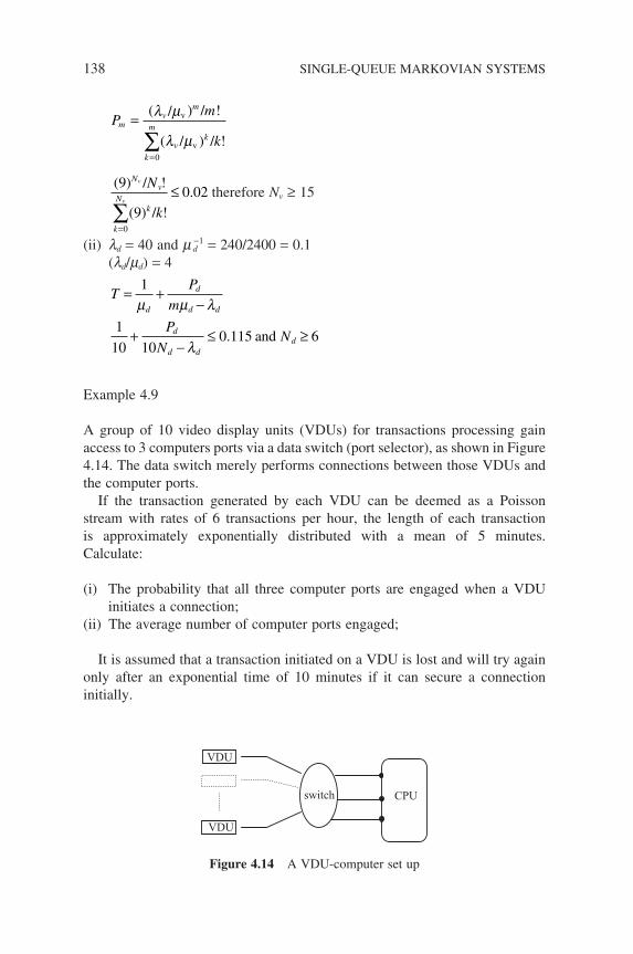
138 SINGLE-QUEUE MARKOVIAN SYSTEMS
Pm
km
vm
k
m
vk
=
=∑( ) / !
( ) / !
λ µ
λ µ
/
/
v
v0
( ) / !
( ) / !.
9
90 02
0
Nv
k
Nk
v
v
N
k=
∑≤ therefore Nv ≥ 15
(ii) ld = 40 and m d−1 = 240/2400 = 0.1 (ld/md) = 4
T
P
md
d
d d
= +−
1
µ µ λ
1
10 100 115 6+
−≤ ≥
P
NNd
d ddλ
. and
Example 4.9
A group of 10 video display units (VDUs) for transactions processing gain access to 3 computers ports via a data switch (port selector), as shown in Figure 4.14. The data switch merely performs connections between those VDUs and the computer ports.
If the transaction generated by each VDU can be deemed as a Poisson stream with rates of 6 transactions per hour, the length of each transaction is approximately exponentially distributed with a mean of 5 minutes. Calculate:
(i) The probability that all three computer ports are engaged when a VDU initiates a connection;
(ii) The average number of computer ports engaged;
It is assumed that a transaction initiated on a VDU is lost and will try again only after an exponential time of 10 minutes if it can secure a connection initially.
switch CPU
VDU
VDU
Figure 4.14 A VDU-computer set up
Solution
In this example, computer ports are servers and transactions are customers and the problem can be formulated as an M/M/m/m system with fi nite arriving customers.
Given l = 6/60 = 0.1 trans/min m−1 = 5 min therefore a = 0.5
(i)
P
k
b
k
k
=
=
=∑
10
30 5
100 5
0 4651
3
0
3
( . )
( . ).
(ii) N =+
× −+
− ×
=
0 5
1 0 510
0 5
1 0 510 3 0 4651
2 248
.
.
.
.( ) .
.
Problems
1. By referring to Section 4.1, show that the variance of N and W for an M/M/1 queue are
(i) Var [N] = r/(1 − r)2
(ii) Var [W] = [m(1 − r)]−2
2. Show that the average number of customers in the M/M/1/S model is N/2 when l = m.
3. Consider an M/M/S/S queueing system where customers arrive from a fi xed population base of S. This system can be modelled as a Markov chain with the following parameters:
λ λµ µ
k
k
s k
k
= −=
( )
Draw the state-transition diagram and show that the probability of an empty system is (1 + r)−S. Hence fi nd the expected number of cus-tomers in the system.
4. Data packets arrive at a switching node, which has only a single output channel, according to a Poisson process with rate l. To handle congestion issues, the switching node implements a simple strategy of dropping incoming packets with a probability p when the total number of packets in the switch (including the one under transmission) is greater or more than N. Assuming that the
CONSIDERATIONS FOR APPLICATIONS OF QUEUEING MODELS 139

140 SINGLE-QUEUE MARKOVIAN SYSTEMS
transmission rate of that output channel is m, fi nd the probability that an arriving packet is dropped by the switch.
5. A trading company intends to install a small PBX to handle ever-increasing internal as well as external calls within the company. It is expected that the employees will collectively generate Poisson out-going external calls with a rate of 30 calls per minute. The duration of these outgoing calls is independent and exponentially distributed with a mean of 3 minutes. Assuming that the PBX has separate external lines to handle the incoming external calls, how many exter-nal outgoing lines are required to ensure that the blocking probability is less than 0.01? You may assume that when an employee receives the busy tone he/she will not make an attempt again.
6. Under what conditions is the assumption ‘Poisson arrival process and exponential service times’ a suitable model for the traffi c offered to a communications link? Show that when ‘Poisson arrival process and exponential service times’ traffi c is offered to a multi-channel communications link with a very large number of channels, the equi-librium carried traffi c distribution (state probability distribution) is Poisson. What is the condition for this system to be stable?
7. Consider Example 4.1 again. If a second doctor is employed to serve the patients, fi nd the average number of patients in the clinic, assum-ing that the arrival and service rates remained the same as before?
8. A trading fi rm has a PABX with two long-distance outgoing trunks. Long-distance calls generated by the employees can be approxi-mated as a Poisson process with rate l. If a call arrives when both trunks are engaged, it will be placed on ‘hold’ until one of the trunks is available. Assume that long-distance calls are exponentially dis-tributed with rate m and the PABX has a large enough capacity to place many calls on hold:
(i) Show that the steady-state probability distribution is 2 11( )−
+ρ
ρρk
(ii) Find the average number of calls in the system.
9. By considering the Engset’s loss system, if there is only one server instead of m servers, derive the probability of having k customers in the system and hence the average number of customers, assuming equilibrium exists.
5Semi-Markovian Queueing Systems
The queueing models that we have discussed so far are all Markovian types; that is both the arrival and service processes are memoryless. These models are appropriate in certain applications but may be inadequate in other instances. For example, in voice communication, the holding time of a call is approxi-mately exponentially distributed, but in the case of packet switching, packets are transmitted either with a fi xed length or a certain limit imposed by the physical constraints. In the latter case, a more appropriate model would be the M/G/1, which belongs to the class of queueing systems called semi-Markovian queueing systems.
Semi-Markovian queueing systems refer to those queueing systems in which either the arrival or service process is not ‘memoryless’. They include M/G/1, G/M/1, their priority queueing variants and, of course, the multi-server counterparts.
In a Markovian queueing system, the stochastic process N(t), t ≥ 0, that is the number of customers in the system at time t, summarizes the complete past history of the system and can be modelled as a birth-death process. This enables us to write down the balance equations from its state transition diagram, and then proceed to calculate Pk and its performance measures.
However, in the case of a semi-Markovian system, say M/G/1, we have to specify the service time already received by the customer in service at time t in addition to the N(t). This is necessary as the distribution of the remaining service time for that customer under service is no longer the same as the origi-nal distribution. The process N(t) no longer possesses the ‘memoryless’
Queueing Modelling Fundamentals Second Edition Ng Chee-Hock and Soong Boon-Hee© 2008 John Wiley & Sons, Ltd
142 SEMI-MARKOVIAN QUEUEING SYSTEMS
property that was discussed in Chapter 2. The concept of fl ow balancing breaks down and we cannot set up simple balance equations for the process N(t), t ≥ 0 using a transition rate diagram.
There are several techniques for solving this type of queueing system. The most frequently presented method in queueing literature is the imbedded Markov-chain approach in which we look at the queue behavior at those instants of a service completion, that is when a customer has fi nished receiving his/her service and left the system. In so doing, we get rid of the remaining service time to the completion of a service interval and again the system can be modelled by a birth-death process. Another approach is the so-called Resid-ual Service Time method which examines the system process from an arriving customer’s perspective. This method is simpler but can only give the mean value of the performance measures.
In this chapter, we present both approaches to highlight the various concepts and theories used in obtaining the results.
5.1 THE M/G/1 QUEUEING SYSTEM
This is a queueing system, Figure 5.1, where customers arrive according to a Poisson process with mean l and are served by a single server of general service-time distribution X(t) (and density function x(t)). We assume that the mean E(x) and the second moment E(x2) of the service time distribution exist and are fi nite. We denote them as x and x2 , respectively.
The capacity of the waiting queue is as usual infi nite and customers are served in the order they arrived, i.e. FCFS. Note that this service discipline will not affect the mean queueing results providing it is work conserving. Simply put, work conserving means that the server does not stay idle when there are customers waiting in the queue. We also assume that the service times are independent of the arrival process as well as the number of customers in the system.
5.1.1 The Imbedded Markov-Chain Approach
As mentioned in the introduction, the stochastic process N(t) is no longer suf-fi cient to completely summarize the past history, as additional information such
λ
general distribution
Figure 5.1 A M/G/1 queueing system
THE M/G/1 QUEUEING SYSTEM 143
as the elapsed service time x0(t) needs to be specifi ed. If we also specify the elapsed service time, then the tuple [N(t), x0(t)] is again a Markov process and we will be able to proceed with the analysis using Markov theory. Unfortu-nately, this is a two-dimensional specifi cation of the state space and compli-cates the analysis considerably.
However, we can simplify the [N(t), x0(t)] specifi cation into a one-dimensional description N(t) by selecting certain special observation instants in time. If we observe the M/G/1 queue at departure instants rn, where x0(t) = 0, then we have a one-dimensional state space specifi cation. The evolu-tion of the number of customers N(t) left behind by a departing customer at these instants is an imbedded Markov chain and we can again resort to Markov theory to derive the desired performance measures.
But before we proceed, let us take a closer look at the state description N(t) at those departure epochs. This is the state probability that is seen by a depart-ing customer. Is it the same as the limiting steady-state probability which is the system state observed by a random observer?
Fortunately, it can be shown that the system state seen by a departing cus-tomer is the same as the system state seen by an arriving customer. Kleinrock (1975) reasoned that the system state in an M/G/1 queue can change at most by +1 or −1. The former corresponds to a customer arrival and the latter refers to a departure. In the long term, the number of transitions upwards must equal the number of transitions downwards. Hence the system state distribution seen by a departing customer should be the same as that seen by an arriving customer.
And according to the PASTA property, as shown in Section 4.2, the system state distribution seen by an arriving customer is the same as the limiting steady-state distribution. We can therefore conclude that the system state dis-tribution that we are going to derive with respect to a departing customer is the same as the limiting steady-state distribution seen by a random observer, that is the usual limiting state distribution we have been deriving for other queues.
With the assurance that the imbedded Markov process will yield the same limiting steady-state distribution, we can then proceed with our analysis.
5.1.2 Analysis of M/G/1 Queue Using Imbedded Markov-Chain Approach
Let us focus our attention at the departure epochs and examine the number of customers Nn left behind by customer Cn at the departure instant rn. If Cn left behind a non-empty system, then customer Cn+1 will leave behind a system with the number of customers increased by the number of arrivals during the service time of customer Cn+1 minus themselves; that is Nn+1 = Nn − 1 + An+1, where An+1 is the number of arrivals during the service time of customer Cn+1.
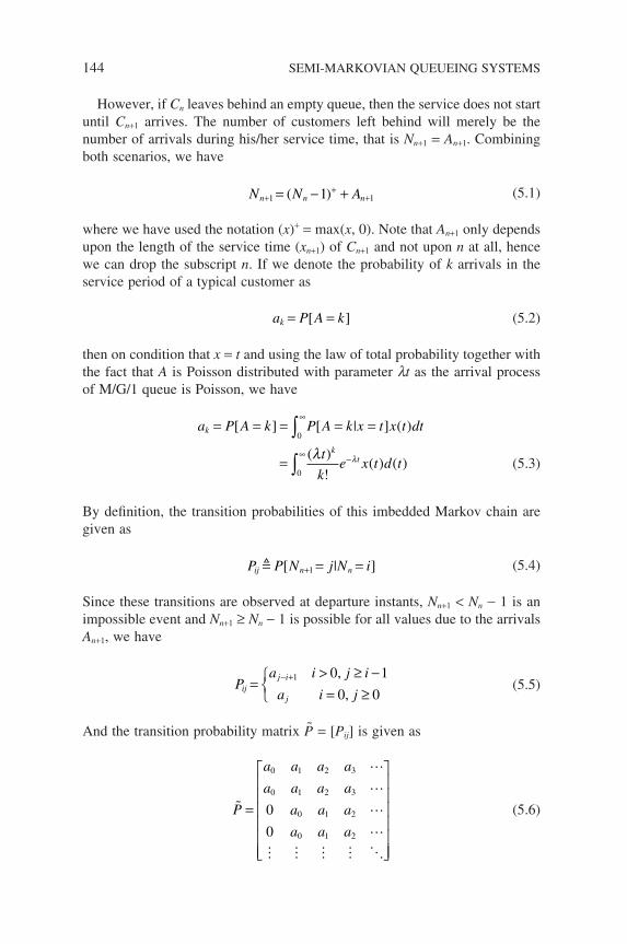
144 SEMI-MARKOVIAN QUEUEING SYSTEMS
However, if Cn leaves behind an empty queue, then the service does not start until Cn+1 arrives. The number of customers left behind will merely be the number of arrivals during his/her service time, that is Nn+1 = An+1. Combining both scenarios, we have
N N An n n++
+= − +1 11( ) (5.1)
where we have used the notation (x)+ = max(x, 0). Note that An+1 only depends upon the length of the service time (xn+1) of Cn+1 and not upon n at all, hence we can drop the subscript n. If we denote the probability of k arrivals in the service period of a typical customer as
a P A kk = =[ ] (5.2)
then on condition that x = t and using the law of total probability together with the fact that A is Poisson distributed with parameter lt as the arrival process of M/G/1 queue is Poisson, we have
a P A k P A k x t x t dt
t
ke x t d t
k
kt
= = = = =
=
∞
∞ −
∫
∫
[ ] [ | ] ( )
( )
!( ) ( )
0
0
λ λ
(5.3)
By defi nition, the transition probabilities of this imbedded Markov chain are given as
P P N j N iij n n [ | ]+ = =1 (5.4)
Since these transitions are observed at departure instants, Nn+1 < Nn − 1 is an impossible event and Nn+1 ≥ Nn − 1 is possible for all values due to the arrivals An+1, we have
Pa i j i
a i jij
j i
j
=> ≥ −= ≥
− +1 0 1
0 0
,
, (5.5)
And the transition probability matrix P = [Pij] is given as
P
a a a a
a a a a
a a a
a a a
=
0 1 2 3
0 1 2 3
0 1 2
0 1 2
0
0
(5.6)
THE M/G/1 QUEUEING SYSTEM 145
Given the service distribution, the transition probabilities are completely defi ned by Equation (5.3) and theoretically the steady state distribution can be found using p = pP. Instead of pursuing this line of analysis, we derive the system state using generating functions. We defi ne the generating function of A as
A z E z P A k zA
k
k( ) [ ] [ ] = ==
∞
∑0
(5.7)
Using Equation (5.3), we have
A zt
ke x t dt z
etz
k
k
kt k
t
k
k
( )( )
!( )
( )
!
= =
=
∞ ∞ −
∞ −
=
∞
∑ ∫
∫ ∑0
0
00
λ
λ
λ
λ
=
= −
∞ − −∫
x t dt
e x t dt
x z
z t
( )
( )
)
( )
0
λ λ
λ λ*(
(5.8)
where x*(l − lz) is the Laplace transform of the service time pdf, x(t), evalu-ated at l − lz.
Expression (5.8) reveals an interesting relationship between the number of arrivals occurring during a service interval x where the arrival process is Poisson at a rate of l.
Let us evaluate the mean and second moment of A as we need them for the subsequent analysis of system state. Using Equation (5.8), we have
A E AdA z
dz
dx z
dz
dx z
d z
d z
d
z
z
[ ]( )
)
( )
( )
( )
=
=−
=−−
⋅−
=
=
1
1
*(
*
λ λ
λ λλ λ
λ λzz
dx z
d z
z
z
=
=
= − ⋅−−
1
1
λ λ λλ λ
*( )
( )
(5.9)
But the last term is just the mean service time x, hence we arrive at
A x= =λ ρ (5.10)
Proceeding with the differentiation further, we can show that
146 SEMI-MARKOVIAN QUEUEING SYSTEMS
A E A
E x A
2 2
2 2
[ ]
[ ]= +λ
(5.11)
5.1.3 Distribution of System State
Let us now return to our earlier investigation of the system state. We defi ne the z-transform of the random variable Nn as
N z E z P N k znN
kn
kn( ) [ ] [ ] = ==
∞
∑0
(5.12)
Taking z-transform of Equation (5.1), we have
E z E zN N An n[ ] [ ]( )++= − +1 1 (5.13)
We drop the subscript of A as it does not depend on n. Note that A is also independent of the random variable Nn, so we can rewrite the previous expression as
E[z Nn+1] = E[z(Nn−1)+]E[zA]
and combining the defi nition of their z-transform, we have
N z A z E ZnNn
+−= ⋅ +
11( ) ( ) [ ]( ) (5.14)
Let us examine the second term on the right-hand side of the expression:
E z P N K z
P N P N K z
N
kn
k
nk
nk
n[ ] [ ]
[ ] [ ]
(
( ) ( )−
=
∞−
=
∞−
+ += =
= = + =
=
∑
∑
1
0
1
1
10
111 1
0
11 1
0
− + = − =
= − + −−
=
∞
∑ρ
ρ ρ
) [ ] [ ]
( ) ( )
zP N K z
zP N
zN z
z
kn
kn
n
(5.15)
We assume that the limiting steady-state exists, that is
N z N z N zn
nn
n( ) ( ) ( )= =→∞ →∞
+lim lim 1
THE M/G/1 QUEUEING SYSTEM 147
We then arrive at
N z
z A z
z A z
z x z
z x z
( ) ( )( ) ( )
( )
( )( ) ( )
( )
= −−−
= −− −− −
11
11
ρ
ρ λ λλ λ
*
*
(5.16)
Having obtained the generating function of the system state given in Equation (5.16), we can proceed to fi nd the mean value N as
N E N td
dzN z z= = =[ ( )] ( )| 1
With N we can proceed to calculate other performance measures of the M/G/1. We will postpone this until we examine the Residual Service Time approach.
5.1.4 Distribution of System Time
System Time refers to the total time a typical customer spends in the system. It includes the waiting time of that customer and its service time. Note that though the distribution of system state derived in the previous sections does not assume any specifi c service discipline, the system time distribution is dependent on the order in which customers are served. Here, we assume that the service discipline is FCFS. The Laplace transform of the system time dis-tribution T(s) can be found using the extension of the concept adopted in the previous section. We will briefl y describe it as this is a commonly used approach in analysing the delays of queueing systems.
Recall that in Section 5.1.2 we derived the generating function of the total arrivals A during a service time interval x, where the arrival process is Poisson with rate l given by A(z) = x*(l − lz). Similarly, since a typical customer spends a system time T in the system, then the total arrivals during their system time interval will be given by
A zt
ke f t dt z
T z
Tk
kt
Tk( )
( )
!( )
)
= = −
=
∞ ∞ −∑ ∫0
0
λ
λ λ
λ
*(
(5.17)
where AT(z) is the generating function of the total arrivals, fT(t) is the density function of system time and T*(s) is the Laplace transform of the system time.
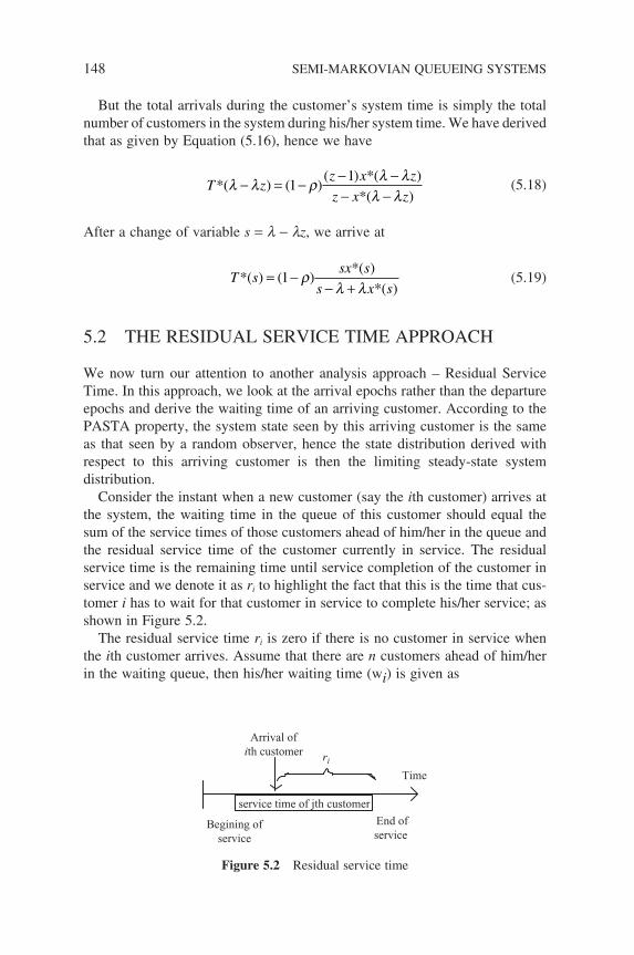
148 SEMI-MARKOVIAN QUEUEING SYSTEMS
But the total arrivals during the customer’s system time is simply the total number of customers in the system during his/her system time. We have derived that as given by Equation (5.16), hence we have
T zz x z
z x z*
*(( ) ( )
( ) *( )
)λ λ ρ λ λ
λ λ− = − − −
− −1
1 (5.18)
After a change of variable s = l − lz, we arrive at
T ssx s
s x s*
*
*( ) ( )
( )
( )= −
− +1 ρ
λ λ (5.19)
5.2 THE RESIDUAL SERVICE TIME APPROACH
We now turn our attention to another analysis approach – Residual Service Time. In this approach, we look at the arrival epochs rather than the departure epochs and derive the waiting time of an arriving customer. According to the PASTA property, the system state seen by this arriving customer is the same as that seen by a random observer, hence the state distribution derived with respect to this arriving customer is then the limiting steady-state system distribution.
Consider the instant when a new customer (say the ith customer) arrives at the system, the waiting time in the queue of this customer should equal the sum of the service times of those customers ahead of him/her in the queue and the residual service time of the customer currently in service. The residual service time is the remaining time until service completion of the customer in service and we denote it as ri to highlight the fact that this is the time that cus-tomer i has to wait for that customer in service to complete his/her service; as shown in Figure 5.2.
The residual service time ri is zero if there is no customer in service when the ith customer arrives. Assume that there are n customers ahead of him/her in the waiting queue, then his/her waiting time (wi) is given as
service time of jth customer
Begining ofservice
End ofservice
Arrival ofith customer
Time
ri
Figure 5.2 Residual service time
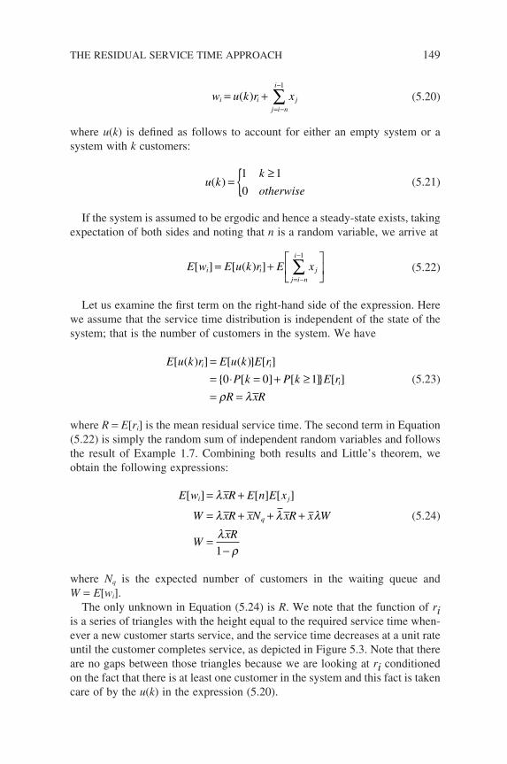
w u k r xi ij i n
i
j= += −
−
∑( )1
(5.20)
where u(k) is defi ned as follows to account for either an empty system or a system with k customers:
u kk
otherwise( ) =
≥1 1
0 (5.21)
If the system is assumed to be ergodic and hence a steady-state exists, taking expectation of both sides and noting that n is a random variable, we arrive at
E w E u k r E xi ij i n
i
j[ ] [ ( ) ]= +
= −
−
∑1
(5.22)
Let us examine the fi rst term on the right-hand side of the expression. Here we assume that the service time distribution is independent of the state of the system; that is the number of customers in the system. We have
E u k r E u k E r
P k P k E r
R xR
i i
i
[ ( ) ] [ ( )] [ ]
[ ] [ ] [ ]
== ⋅ = + ≥= =
0 0 1
ρ λ (5.23)
where R = E[ri] is the mean residual service time. The second term in Equation (5.22) is simply the random sum of independent random variables and follows the result of Example 1.7. Combining both results and Little’s theorem, we obtain the following expressions:
E w xR E n E x
W xR xN xR x W
WxR
i j
q
[ ] [ ] [ ]= +
= + + +
=−
λ
λ λ λλ
ρ1
(5.24)
where Nq is the expected number of customers in the waiting queue and W = E[wi].
The only unknown in Equation (5.24) is R. We note that the function of ri is a series of triangles with the height equal to the required service time when-ever a new customer starts service, and the service time decreases at a unit rate until the customer completes service, as depicted in Figure 5.3. Note that there are no gaps between those triangles because we are looking at ri conditioned on the fact that there is at least one customer in the system and this fact is taken care of by the u(k) in the expression (5.20).
THE RESIDUAL SERVICE TIME APPROACH 149
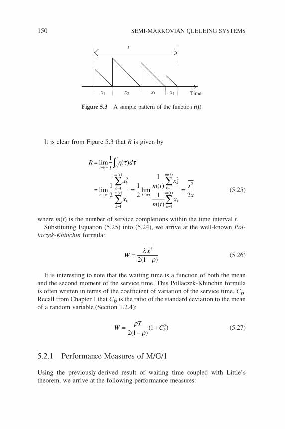
150 SEMI-MARKOVIAN QUEUEING SYSTEMS
It is clear from Figure 5.3 that R is given by
Rt
r d
x
x
t
t
i
t
k
m t
k
k
m t
k
t
=
= =
→∞
→∞
=
=
→
∫
∑
∑
lim
lim lim
1
1
2
1
2
0
1
2
1
( )
( )
( )
τ τ
∞∞
=
=
∑
∑=
1
1 21
2
1
2m tx
m tx
x
xk
m t
k
k
m t
k
( )
( )
( )
( )
(5.25)
where m(t) is the number of service completions within the time interval t.Substituting Equation (5.25) into (5.24), we arrive at the well-known Pol-
laczek-Khinchin formula:
Wx=−
λρ
2
2 1( ) (5.26)
It is interesting to note that the waiting time is a function of both the mean and the second moment of the service time. This Pollaczek-Khinchin formula is often written in terms of the coeffi cient of variation of the service time, Cb. Recall from Chapter 1 that Cb is the ratio of the standard deviation to the mean of a random variable (Section 1.2.4):
Wx
Cb=−
+ρρ2 1
1 2
( )( ) (5.27)
5.2.1 Performance Measures of M/G/1
Using the previously-derived result of waiting time coupled with Little’s theorem, we arrive at the following performance measures:
Timex1 x2 x3 x4
t
Figure 5.3 A sample pattern of the function r(t)
(i) The number of customers in the waiting queue:
N Wx
q = =−
λ λρ
2 2
2 1( ) (5.28)
(ii) The time spent in the system (system time):
T xx= +−
λρ
2
2 1( ) (5.29)
(iii) The number of customers in the system:
Nx= +−
ρ λρ
2 2
2 1( ) (5.30)
A special case of the M/G/1 queueing system is that of deterministic service time – the M/D/1 model. This particular queueing system is a good model for analysing packet delays of an isolated queue in a packet switching network if the packet arrival process is Poisson. This model has been used to analyse the performance of time-division multiplexing and asynchronous time-division multiplexing.
Another important application of M/G/1 queueing systems in communica-tions networks is in the study of data link protocols, for example, Stop-and-Wait and Sliding Window protocols.
Example 5.1
Let us re-visit the train arrivals problem of Example 2.4. If the arrival process is not Poisson and the inter-train arrival times are distributed according to a general distribution with a mean of 10 minutes, when a passenger arrives at the station, how long does he/she need to wait on average until the next train arrives?
Solution
Intuitively, you may argue that since you may likely to come at the middle of an inter-arrival interval, hence the answer is 5 minutes. The actual answer is somewhat counter-intuitive to the above intuitive reasoning. Let us examine the situation more closely.
THE RESIDUAL SERVICE TIME APPROACH 151
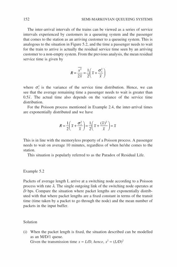
152 SEMI-MARKOVIAN QUEUEING SYSTEMS
The inter-arrival intervals of the trains can be viewed as a series of service intervals experienced by customers in a queueing system and the passenger that comes to the station as an arriving customer to a queueing system. This is analogous to the situation in Figure 5.2, and the time a passenger needs to wait for the train to arrive is actually the residual service time seen by an arriving customer to a non-empty system. From the previous analysis, the mean residual service time is given by
Rx
xx
xx= = +
2 2
2
1
2
σ
where s 2x is the variance of the service time distribution. Hence, we can
see that the average remaining time a passenger needs to wait is greater than 0.5x . The actual time also depends on the variance of the service time distribution.
For the Poisson process mentioned in Example 2.4, the inter-arrival times are exponentially distributed and we have
R xx
xx
xxx= +
= +
=
1
2
1
2
2 2σ ( )
This is in line with the memoryless property of a Poisson process. A passenger needs to wait on average 10 minutes, regardless of when he/she comes to the station.
This situation is popularly referred to as the Paradox of Residual Life.
Example 5.2
Packets of average length L arrive at a switching node according to a Poisson process with rate l. The single outgoing link of the switching node operates at D bps. Compare the situation where packet lengths are exponentially distrib-uted with that where packet lengths are a fi xed constant in terms of the transit time (time taken by a packet to go through the node) and the mean number of packets in the input buffer.
Solution
(i) When the packet length is fi xed, the situation described can be modelled as an M/D/1 queue.Given the transmission time x = L/D, hence, x2 = (L/D)2
We have TL
D
L D
L D
L D
L D
L D
L D
NL
D
L
= +−
=−
−−
= +
λλ
λλ
λ
λ λ
( / )
( / )
/
/
( / )
( / )
(
2
2
2
2 1
1 2 1
// )
( / )
( / )
/ )
( / )
( / )
D
L D
L D
L D
L D
L D
2
2 2
2 1
1 2 1
−
=−
−−
λλλ
λλ
(ii) When the packet lengths are exponentially distributed, it is an M/M/1 model, and we have
TL D
L D
NL D
L D
=−
=−
/
/
( / )
/
1
1
λ
λλ
We see that the constant service time case offers better performance than the exponential case as far as the transit time and number of messages in the system are concerned.
Example 5.3
In a point-to-point setup as shown in Figure 5.4, data packets generated by device A are sent over a half-duplex transmission channel operating at 64 Kbps using stop-and-wait protocol. Data packets are assumed to be gener-ated by the device according to a Poisson process and are of fi xed length of 4096 bits. The probability of a packet being in error is 0.01 and the round trip propagation delay is a constant 10 msec. Assume that Acks and Nacks are never in error.
A B
64 kbps
Half-duplex
A point-to-point setup
Figure 5.4 A point-to-point setup
THE RESIDUAL SERVICE TIME APPROACH 153
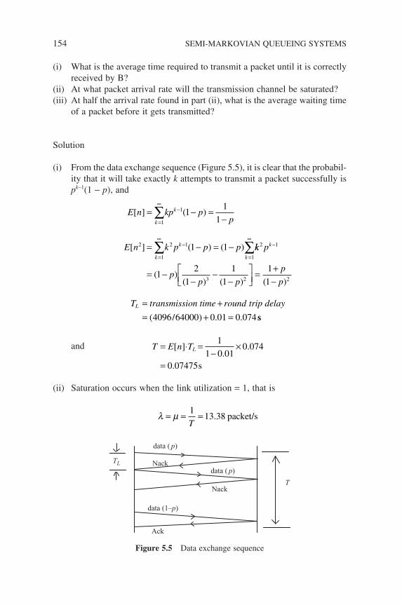
154 SEMI-MARKOVIAN QUEUEING SYSTEMS
(i) What is the average time required to transmit a packet until it is correctly received by B?
(ii) At what packet arrival rate will the transmission channel be saturated?(iii) At half the arrival rate found in part (ii), what is the average waiting time
of a packet before it gets transmitted?
Solution
(i) From the data exchange sequence (Figure 5.5), it is clear that the probabil-ity that it will take exactly k attempts to transmit a packet successfully is pk−1(1 − p), and
E n kp pp
E n k p p p
k
k
k
k
k
[ ] ( )
[ ] ( ) ( )
= − =−
= − = −
=
∞−
=
∞−
=
∞
∑
∑ ∑
1
1
2
1
2 1
1
11
1
1 1 kk p
pp p
p
p
k2 1
3 2 21
2
1
1
1
1
1
−
= −−
−−
= +
−( )
( ) ( ) ( )
T transmission time round trip delayL = += + =( / ) . .4096 64000 0 01 0 074ss
and T E n TL= ⋅ =−
×
=
[ ].
.
.
1
1 0 010 074
0 07475s
(ii) Saturation occurs when the link utilization = 1, that is
λ µ= = =113 38
T. packet/s
data ( p)
data (1–p)
data ( p)
Nack
Nack
Ack
TL
T
Figure 5.5 Data exchange sequence
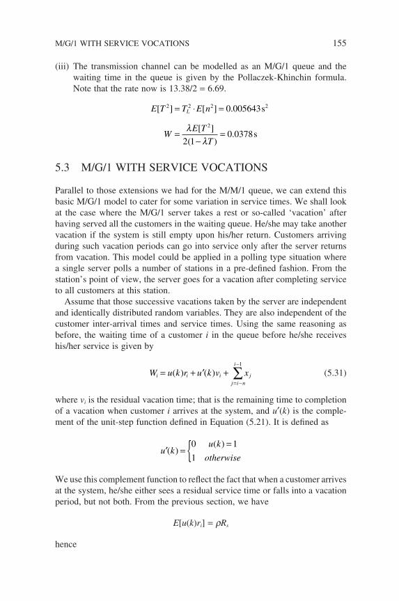
(iii) The transmission channel can be modelled as an M/G/1 queue and the waiting time in the queue is given by the Pollaczek-Khinchin formula. Note that the rate now is 13.38/2 = 6.69.
E T T E n
WE T
T
L[ ] [ ] .
[ ]
( ).
2 2 2 2
2
0 005643
2 10 0378
= ⋅ =
=−
=
s
sλ
λ
5.3 M/G/1 WITH SERVICE VOCATIONS
Parallel to those extensions we had for the M/M/1 queue, we can extend this basic M/G/1 model to cater for some variation in service times. We shall look at the case where the M/G/1 server takes a rest or so-called ‘vacation’ after having served all the customers in the waiting queue. He/she may take another vacation if the system is still empty upon his/her return. Customers arriving during such vacation periods can go into service only after the server returns from vacation. This model could be applied in a polling type situation where a single server polls a number of stations in a pre-defi ned fashion. From the station’s point of view, the server goes for a vacation after completing service to all customers at this station.
Assume that those successive vacations taken by the server are independent and identically distributed random variables. They are also independent of the customer inter-arrival times and service times. Using the same reasoning as before, the waiting time of a customer i in the queue before he/she receives his/her service is given by
W u k r u k v xi i ij i n
i
j= + ′ += −
−
∑( ) ( )1
(5.31)
where vi is the residual vacation time; that is the remaining time to completion of a vacation when customer i arrives at the system, and u′(k) is the comple-ment of the unit-step function defi ned in Equation (5.21). It is defi ned as
′ ==u k
u k
otherwise( )
( )0 1
1
We use this complement function to refl ect the fact that when a customer arrives at the system, he/she either sees a residual service time or falls into a vacation period, but not both. From the previous section, we have
E[u(k)ri] = rRs
hence
M/G/1 WITH SERVICE VOCATIONS 155
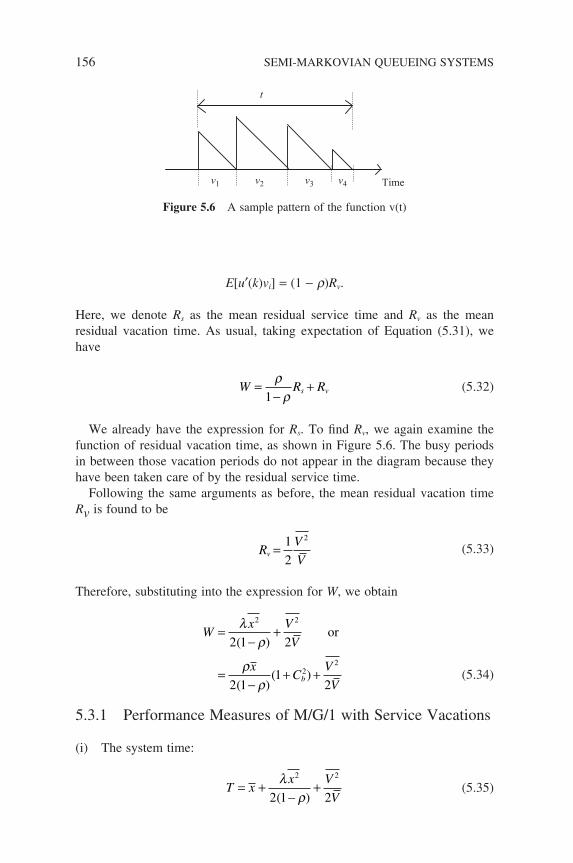
156 SEMI-MARKOVIAN QUEUEING SYSTEMS
E[u′(k)vi] = (1 − r)Rv.
Here, we denote Rs as the mean residual service time and Rv as the mean residual vacation time. As usual, taking expectation of Equation (5.31), we have
W R Rs v=−
+ρρ1
(5.32)
We already have the expression for Rs. To fi nd Rv, we again examine the function of residual vacation time, as shown in Figure 5.6. The busy periods in between those vacation periods do not appear in the diagram because they have been taken care of by the residual service time.
Following the same arguments as before, the mean residual vacation time Rv is found to be
RV
Vv =
1
2
2
(5.33)
Therefore, substituting into the expression for W, we obtain
Wx V
V
xC
V
Vb
=−
+
=−
+ +
λρ
ρρ
2 2
22
2 1 2
2 11
2
( )
( )( )
or
(5.34)
5.3.1 Performance Measures of M/G/1 with Service Vacations
(i) The system time:
T xx V
V= +
−+λ
ρ
2 2
2 1 2( ) (5.35)
Timev1 v2 v3 v4
t
Figure 5.6 A sample pattern of the function v(t)
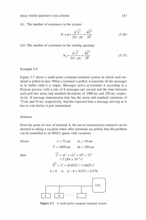
(ii) The number of customers in the system:
Nx V
V= +
−+ρ λ
ρλ2 2 2
2 1 2( ) (5.36)
(iii) The number of customers in the waiting queuing:
Nx V
Vq = −
+λρ
λ2 2 2
2 1 2( ) (5.37)
Example 5.4
Figure 5.7 shows a multi-point computer-terminal system in which each ter-minal is polled in turn. When a terminal is polled, it transmits all the messages in its buffer until it is empty. Messages arrive at terminal A according to a Poisson process with a rate of 8 messages per second and the time between each poll has mean and standard deviations of 1000 ms and 250 ms, respec-tively. If message transmission time has the mean and standard variations of 72 ms and 10 ms, respectively, fi nd the expected time a message arriving at A has to wait before it gets transmitted.
Solution
From the point of view of terminal A, the server (transmission channel) can be deemed as taking a vacation when other terminals are polled, thus the problem can be modelled as an M/G/1 queue with vacations:
Given: x = 72 ms s x = 10 ms
V = 1000 ms sV = 250 ms
then x2 = s 2 + (x)2 = 102 + 722
= 5.284 × 10⁻³ s2
V 2 = 12 + (0.025)2 = 1.0625 s2
l = 8 ⇒ r − 8 × 0.072 = 0.576
A B
CPU
Figure 5.7 A multi-point computer terminal system
M/G/1 WITH SERVICE VOCATIONS 157
158 SEMI-MARKOVIAN QUEUEING SYSTEMS
Therefore, we have
Wx V
V=
−+ =λ
ρ
2 2
2 1 20 581
( ). s
5.4 PRIORITY QUEUEING SYSTEMS
For all the queueing systems that we have discussed so far, the arriving customers are treated equally and served in the order they arrive at the system; that is FCFS queueing discipline is assumed. However, in real life we often encounter situations where certain customers are more important than others. They are given greater privileges and receive their services before others. The queueing system that models this kind of situation is called a priority queueing system.
There are various applications of this priority model in data networks. In a packet switching network, control packets that carry vital instructions for network operations are usually transmitted with a higher priority over that of data packets. In a multi-media system in which voice and data are carried in the same network, the voice packets may again accord a higher priority than that of the data packets owing to real-time requirements.
For our subsequent treatments of priority queueing systems, we divide the arriving customers into n different priority classes. The smaller the priority class number, the higher the priority; i.e. Class 1 has the highest priority and Class 2 has the second highest and so on.
There are two basic queueing disciplines for priority systems, namely pre-emptive and non-preemptive. In a pre-emptive priority queueing system, the service of a customer is interrupted when a customer of a higher priority class arrives. As a further division, if the customer whose service was interrupted resumes service from the point of interruption once all customers of higher priority have been served, it is a pre-emptive resume system. If the customer repeats his/her entire service, then it is a pre-emptive repeat system. In the case of the non-preemptive priority system, a customer’s service is never inter-rupted, even if a customer of higher priority arrives in the meantime.
5.4.1 M/G/1 Non-preemptive Priority Queueing
We shall begin with the analysis of an M/G/1 non-preemptive system. In this model, customers of each priority Class i (i = 1, 2, . . . n) arrive according to a Poisson process with rate li and are served by the same server with a general service time distribution of mean xi and second moment xi
2 for customers of each Class i, as shown in Figure 5.8. The arrival process of each class is assumed to be independent of each other and the service process. Within each
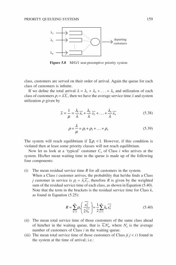
class, customers are served on their order of arrival. Again the queue for each class of customers is infi nite.
If we defi ne the total arrival l = l1 + l2 + . . . + ln and utilization of each class of customers ri = l xi , then we have the average service time x and system utilization r given by
x x x xnn= = + + +1 1
12
2µλλ
λλ
λλ
. . . (5.38)
ρ λµ
ρ ρ ρ= = + + +1 2 . . . n (5.39)
The system will reach equilibrium if Σρi < 1. However, if this condition is violated then at least some priority classes will not reach equilibrium.
Now let us look at a ‘typical’ customer Cn of Class i who arrives at the
system. His/her mean waiting time in the queue is made up of the following four components:
(i) The mean residual service time R for all customers in the system.When a Class i customer arrives, the probability that he/she fi nds a Class j customer in service is rj = lj x j , therefore R is given by the weighted sum of the residual service time of each class, as shown in Equation (5.40). Note that the term in the brackets is the residual service time for Class k, as found in Equation (5.25):
Rx
xx
k
n
kk
k k
n
k k=
=
= =∑ ∑
1
2
1
2
2
1
2ρ λ (5.40)
(ii) The mean total service time of those customers of the same class ahead of him/her in the waiting queue, that is xi Ni
q, where Niq is the average
number of customers of Class i in the waiting queue.(iii) The mean total service time of those customers of Class j( j < i ) found in
the system at the time of arrival; i.e.:
λ1
λi
λn
departingcustomers
Figure 5.8 M/G/1 non-preemptive priority system
PRIORITY QUEUEING SYSTEMS 159
160 SEMI-MARKOVIAN QUEUEING SYSTEMS
j
i
j qjx N
=
−
∑1
1
.
(iv) The mean total service time of those customers of Class j( j < i) arriving at the system while customer Cn is waiting in the queue, i.e.:
j
i
j j ix W=
−
∑1
1
λ
Combining the four components together, we arrive at
W R x N x N x Wi i qi
j
i
j qj
j
i
j j i= + + +=
−
=
−
∑ ∑1
1
1
1
λ (5.41)
For Class 1 customers, since their waiting times are not affected by custom-ers of lower classes, the expression of W1 is the same as that of an M/G/1 queue and is given by
WR
111
=− ρ
(5.42)
By using Equation (5.41) together with Equation (5.42) and the expression Nk
q = lkWk, we can obtain the mean waiting time for Class 2 customers as
WR
21 1 21 1
=− − −( )( )ρ ρ ρ
(5.43)
In general, the expression for the mean waiting time for Class i customers can be calculated recursively using the preceding approach and it yields
WR
ii i
=− − − − − −−( )( )1 11 2 1 1 2ρ ρ ρ ρ ρ ρ. . . . . .
(5.44)
where the mean residual service time R is given by expression (5.40).
5.4.2 Performance Measures of Non-preemptive Priority
The other performance measures can be found once the waiting time is known:
(i) The average number of customers of each class in their own waiting queue:
( )( )( )
N WR
q i i ii
i
= =− − − − − −−
λ λρ ρ ρ ρ1 11 1 1 1. . . . . .
(5.45)
(ii) The total time spends in the system by a customer of Class i:
T W xi i i= + (5.46)
(iii) Total number of customers in the system:
N Nk
n
q k= +=∑
1
( ) ρ (5.47)
(iv) If the service times of each class of customers are exponentially distrib-uted with a mean of m, then in effect we have an M/M/1 non-preemptive priority system. Then we have
Rk
n
k=
=
=∑1
2
1
1
2
λµ
ρµ
(5.48)
Note that the variance and mean of an exponential distribution with parameter m are m−2 and m−1, respectively, hence the second moment is 2m−2.
Example 5.5
In a packet switching network, there are two types of packets traversing the network; namely data packets of fi xed length of 4800 bits and control packets of fi xed length of 192 bits. On average, there are 15% control packets and 85% data packets present in the network and the combined arriving stream of packets to a switching node is Poisson with rate l = 4 packets per second. If all transmission links in the network operate at 19.2 kbps, calculate:
(i) the average waiting time for both the control and data packets at a switch-ing node.
(ii) the waiting times for the control and data packets respectively if a non-preemptive priority scheme is employed at each switching node with control packets given a higher priority.
PRIORITY QUEUEING SYSTEMS 161
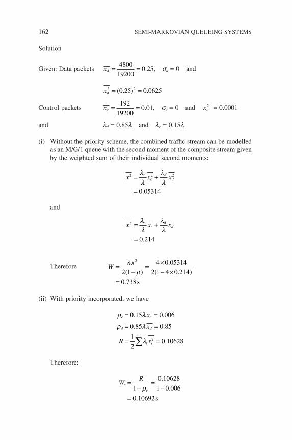
162 SEMI-MARKOVIAN QUEUEING SYSTEMS
Solution
Given: Data packets xd = =4800
192000 25. , sd = 0 and
xd2 20 25 0 0625= =( . ) .
Control packets xc = =192
192000 01. , sc = 0 and xc
2 = 0.0001
and ld = 0.85l and lc = 0.15l
(i) Without the priority scheme, the combined traffi c stream can be modelled as an M/G/1 queue with the second moment of the composite stream given by the weighted sum of their individual second moments:
x x xcc
dd
2 2 2
0 05314
= +
=
λλ
λλ
.
and
x x xcc
dd
2
0 214
= +
=
λλ
λλ
.
Therefore Wx=−
= ×− ×
=
λρ
2
2 1
4 0 05314
2 1 4 0 214
0 738
( )
.
( . )
. s
(ii) With priority incorporated, we have
ρ λ
ρ λ
λ
c c
d d
i i
x
x
R x
= =
= =
= =∑
0 15 0 006
0 85 0 85
1
20 106282
. .
. .
.
Therefore:
WR
cc
=−
=−
=1
0 10628
1 0 006
0 10692
ρ.
.
. s
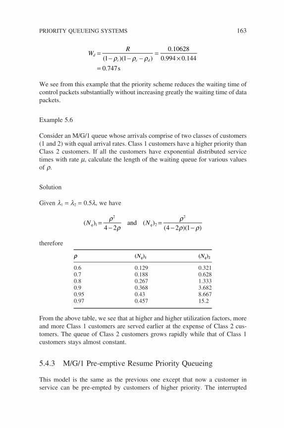
WR
dc c d
=− − −
=×
=( )( )
.
. .
.
1 1
0 10628
0 994 0 144
0 747
ρ ρ ρs
We see from this example that the priority scheme reduces the waiting time of control packets substantially without increasing greatly the waiting time of data packets.
Example 5.6
Consider an M/G/1 queue whose arrivals comprise of two classes of customers (1 and 2) with equal arrival rates. Class 1 customers have a higher priority than Class 2 customers. If all the customers have exponential distributed service times with rate m, calculate the length of the waiting queue for various values of r.
Solution
Given l1 = l2 = 0.5l, we have
( ) ( )( )( )
N Nq q1
2
2
2
4 2 4 2 1=
−=
− −ρρ
ρρ ρ
and
therefore
r (Nq)1 (Nq)2
0.6 0.129 0.3210.7 0.188 0.6280.8 0.267 1.3330.9 0.368 3.6820.95 0.43 8.6670.97 0.457 15.2
From the above table, we see that at higher and higher utilization factors, more and more Class 1 customers are served earlier at the expense of Class 2 cus-tomers. The queue of Class 2 customers grows rapidly while that of Class 1 customers stays almost constant.
5.4.3 M/G/1 Pre-emptive Resume Priority Queueing
This model is the same as the previous one except that now a customer in service can be pre-empted by customers of higher priority. The interrupted
PRIORITY QUEUEING SYSTEMS 163
164 SEMI-MARKOVIAN QUEUEING SYSTEMS
service resumes from the point of interruption when all customers of higher priority classes have been served. There are two basic distinctions between this mode and the previous one:
(i) The presence of customers of lower priority Classes (i + 1 to n) in the system has no effect on the waiting time of a customer of Class i because he/she always pre-empts those customers of lower priority classes. So in the analysis, we can ignore those customers of Class i + 1 to n.
(ii) While a customer of Class i is waiting for his/her service, his/her waiting time is the same whether customers of Class 1 to i − 1 are served in a pre-emptive manner or non-preemptive fashion. This is due to the fact that he/she only gets his/her service when there are no customers of higher priority classes in the system.
We can use the expression (5.44) for his/her waiting time. Thus, the waiting time in queue of a customer of Class i is given by
WR
R xii
i ii
k
i
k k=− − − − − −
=− =
∑( )( )1 1
1
21 1 1 1
2
ρ ρ ρ ρλ
. . . . . .and (5.49)
However, the system time of a customer of Class i is not equal to Wi plus his/her service time because his/her service may be interrupted by customers of higher Classes (1 to i − 1) arriving while he/she is being served. Let us defi ne T k′ to be the time his/her service starts until completion, then we have the fol-lowing expression:
′= + ′=
−
∑T x x Ti ij
i
j j i1
1
( )λ (5.50)
where ljTi′ is the average arrival of customers of Class j ( j = 1 to i − 1) during the time Ti′. Combining these two parts, the system time of a customer of Class i is then given by
T W T
TR x
i i i
ii
i i i
i
i
= + ′
=− − − − − −
+− − −− −( )( ) (1 1 11 1 1ρ ρ ρ ρ ρ ρ. . . . . . . . . 11)
(5.51)
and we arrive at the following expression:
Tx R
iii i
i i
= − − − +− − − − − −
>−
( )
( )( )
1
1 111 1
1 1 1
ρ ρρ ρ ρ ρ
. . .
. . . . . . (5.52)
For i = 1, we have
Tx R
11 1 1
1
1
1= − +
−( )ρ
ρ (5.53)
Example 5.7
Consider Example 5.5, we repeat the calculation assuming the pre-emptive resume priority scheme is employed.
Solution
R x
R x x
Tx R
c c
c c d d
cc c
12
22 2
1
1
20 00003
1
20 10628
1
= =
= + =
= − +
λ
λ λ
ρ
.
( ) .
( )
110 01003
1
1 10 9942
−=
= − − +− − −
=
ρ
ρ ρρ ρ ρ
c
dd c d
c c d
Tx R
.
( )
( )( ).
s
s
Compare them with that of the non-preemptive scheme:
T W x
T W xc c c
d d d
= + == + =
0 11692
0 9925
.
.
s
s
Again, we see that the pre-emptive scheme signifi cantly reduces the system time of the control packets without increasing too much the system time of those data packets.
5.5 THE G/M/1 QUEUEING SYSTEM
The G/M/1 queueing system can be considered as the ‘dual image’ of M/G/1. This model is less useful than M/G/1 in data networks, owing to the reasons given in Section 4.8. However, it is important theoretically and worth mention-ing because this is the fi rst time (in so many chapters) that we see that the system state seen by an arriving customer is different from that seen by a random observer.
THE G/M/1 QUEUEING SYSTEM 165
166 SEMI-MARKOVIAN QUEUEING SYSTEMS
In this model, customers arrive according to a general arrival process with mean rate l and are served by an exponential server with mean m−1. The inter-arrival times of those customers are assumed to be independent and identically distributed random variables. Some literature uses GI instead of G to signify this nature of independence.
The stochastic process N(t) is not Markovian because the elapsed time since the last arrival has to be considered in deriving Pk. But if we focus our attention at those instants where an arrival occurs, the process N(t)|An arrival at those arrival instants can be shown to be a Markovian process and so solved by the imbedded Markov-chain technique.
We will not discuss the analysis of this model as it is rather complex, but just state the results. It has been shown (Kleinrock 1975) that the probability of fi nding k customers in the system immediately before an arrival is given by the following:
R kkk= − =( )1 0 2σ σ ,1, , . . . (5.54)
where s is the unique root of the equation:
σ µ µσ= −A*( ) (5.55)
and A*(m − ms) denotes the Laplace transform of the pdf of inter-arrival times evaluated at the special point (m − ms ).
As discussed earlier, Rk is, in general, not equal to Pk. They are equal only when the arrival process is Poisson. It can be shown that Pk is given by
PR k
kk
k==
− = −ρρ
1 1 2 3
1 0
, , , . . . (5.56)
5.5.1 Performance Measures of GI/M/1
(i) The number of customers in the waiting queue:
N kP kq
kk
k
k= + −
=−
=
∞
+=
∞
∑ ∑0
11
1
1
ρ σ σ
ρσσ
( )
(5.57)
(ii) The number of customers in the system:
N kPk
k= =−=
∞
∑0 1
ρσ
(5.58)
(iii) The waiting time in the queue:
WNq= =
−λσ
µ σ( )1 (5.59)
(iv) The time spent in the system:
TN= =
−λ µ σ1
1( ) (5.60)
Problems
1. Consider a switch with two input links and one outgoing transmission link. Data packets arrive at the fi rst input link according to a Poisson process with mean l1 and voice packets arrive at the second input link also according to a Poisson process with mean l2. Determine the total transit time when a packet arrives at either input until its transmission completion if the service time of both the data and voice packets are exponentially distributed with mean rates m1 and m2, respectively.
2. Consider a time-division multiplexor that multiplexes 30 input packet streams onto a outgoing link with a slot time of 4 ms. Assume that the packet arrival process of each packet stream is Poisson with a rate of 3000 packets/sec. What is the average waiting time before a packet is transmitted if the outgoing link transmits a packet from each input line and then instantaneously switches to serve the next input line according to a fi xed service cycle?
3. Two types of packets, naming Control and Data packets, arrive at a switching node as independent Poisson processes with a rate of 10 packets/sec (Control packets) and 30 packets/sec (Data packets), respectively. Control packets have a constant length of 80 bits and are given higher priority over Data packets for processing. Data packets are of exponential length with a mean of 1000 bits. If the only outgoing link of this node is operating at 64 000 bps, determine the mean waiting times of these two types of packets for a non-preemptive priority system. Repeat the calculation when the priorities of these two types of packets are switched.
4. Repeat Question 3 if the pre-emptive priority system is used.5. Consider a queueing system where customers arrive according to a
Poisson process with rate l but the service facility now consists of two servers in series. A customer upon entry into the service facility will spend a random amount of time with server 1, and then proceeds
THE G/M/1 QUEUEING SYSTEM 167
168 SEMI-MARKOVIAN QUEUEING SYSTEMS
immediately to the second server for service after leaving server 1. While the customer in the service facility is receiving his/her service from either server, no other customer is allowed into the service facility. If the service rates of these two servers are exponentially distributed with rate 2m, calculate the mean waiting time of a cus-tomer in this queueing system.
6. Consider the queueing system in Problem 5, but the service facility now consists of two parallel servers instead of serial servers. A cus-tomer upon entry into the service facility will proceed to either server 1 with probability 0.25 or to server 2 with probability 0.75. While the customer in the service facility is receiving his/her service, no other customer is allowed into the service facility. If the service rates of these two servers are exponentially distributed with rate mi(i = 1,2), calculate the mean waiting time of a customer in this queueing system.
6Open Queueing Networks
In preceding discussions, we have dealt solely with single isolated queueing systems and showed examples of their applications in data networks. It is a natural extension to now look at a collection of interactive queueing systems, the so-called networks of queues, whereby the departures of some queues feed into other queues. In fact, queueing networks are a more realistic model for a system with many resources interacting with each other. For simplicity, each individual queueing system is often referred to as a queue in a queueing network or just a node. We will use this terminology when the context is clear.
The analysis of a queueing network is much more complicated due to the interactions between various queues and we have to examine them as a whole. The state of one queue is generally dependent on the others because of feedback loops and hence the localized analysis of an isolated queue will not give us a complete picture of the network dynamics.
There are many real-life applications that can be modelled as networks of queues. In communication networks, those cascaded store-and-forward switch-ing nodes that forward data packets/messages from one node to another are a good example of a network of queues. Job processing on a machine fl oor is another candidate for the model of network queues. A job usually requires a sequence of operations by one or more machines. A job entering the machine fl oor corresponds to an arrival, and its departure occurs when its required pro-cessing at various machines has been completed.
There are various ways of classifying queueing networks. From the network topology point of view, queueing networks can be categorized into two generic classes, namely Open and Closed Queueing Networks, and of course a mixture
Queueing Modelling Fundamentals Second Edition Ng Chee-Hock and Soong Boon-Hee© 2008 John Wiley & Sons, Ltd
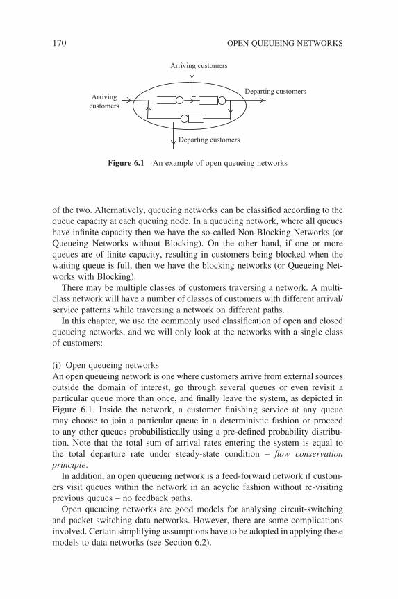
170 OPEN QUEUEING NETWORKS
of the two. Alternatively, queueing networks can be classifi ed according to the queue capacity at each queuing node. In a queueing network, where all queues have infi nite capacity then we have the so-called Non-Blocking Networks (or Queueing Networks without Blocking). On the other hand, if one or more queues are of fi nite capacity, resulting in customers being blocked when the waiting queue is full, then we have the blocking networks (or Queueing Net-works with Blocking).
There may be multiple classes of customers traversing a network. A multi-class network will have a number of classes of customers with different arrival/service patterns while traversing a network on different paths.
In this chapter, we use the commonly used classifi cation of open and closed queueing networks, and we will only look at the networks with a single class of customers:
(i) Open queueing networksAn open queueing network is one where customers arrive from external sources outside the domain of interest, go through several queues or even revisit a particular queue more than once, and fi nally leave the system, as depicted in Figure 6.1. Inside the network, a customer fi nishing service at any queue may choose to join a particular queue in a deterministic fashion or proceed to any other queues probabilistically using a pre-defi ned probability distribu-tion. Note that the total sum of arrival rates entering the system is equal to the total departure rate under steady-state condition – fl ow conservation principle.
In addition, an open queueing network is a feed-forward network if custom-ers visit queues within the network in an acyclic fashion without re-visiting previous queues – no feedback paths.
Open queueing networks are good models for analysing circuit-switching and packet-switching data networks. However, there are some complications involved. Certain simplifying assumptions have to be adopted in applying these models to data networks (see Section 6.2).
Arrivingcustomers
Departing customers
Arriving customers
Departing customers
Figure 6.1 An example of open queueing networks
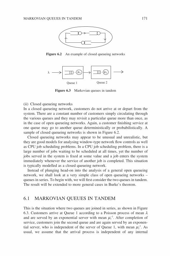
MARKOVIAN QUEUES IN TANDEM 171
(ii) Closed queueing networksIn a closed queueing network, customers do not arrive at or depart from the system. There are a constant number of customers simply circulating through the various queues and they may revisit a particular queue more than once, as in the case of open queueing networks. Again, a customer fi nishing service at one queue may go to another queue deterministically or probabilistically. A sample of closed queueing networks is shown in Figure 6.2.
Closed queueing networks may appear to be unusual and unrealistic, but they are good models for analysing window-type network fl ow controls as well as CPU job scheduling problems. In a CPU job scheduling problem, there is a large number of jobs waiting to be scheduled at all times, yet the number of jobs served in the system is fi xed at some value and a job enters the system immediately whenever the service of another job is completed. This situation is typically modelled as a closed queueing network.
Instead of plunging head-on into the analysis of a general open queueing network, we shall look at a very simple class of open queueing networks – queues in series. To begin with, we will fi rst consider the two queues in tandem. The result will be extended to more general cases in Burke’s theorem.
6.1 MARKOVIAN QUEUES IN TANDEM
This is the situation where two queues are joined in series, as shown in Figure 6.3. Customers arrive at Queue 1 according to a Poisson process of mean l and are served by an exponential server with mean m1
−1. After completion of service, customers join the second queue and are again served by an exponen-tial server, who is independent of the server of Queue 1, with mean m2
−1. As usual, we assume that the arrival process is independent of any internal
Figure 6.2 An example of closed queueing networks
Queue 1 Queue 2
λ µ1 µ2
Figure 6.3 Markovian queues in tandem
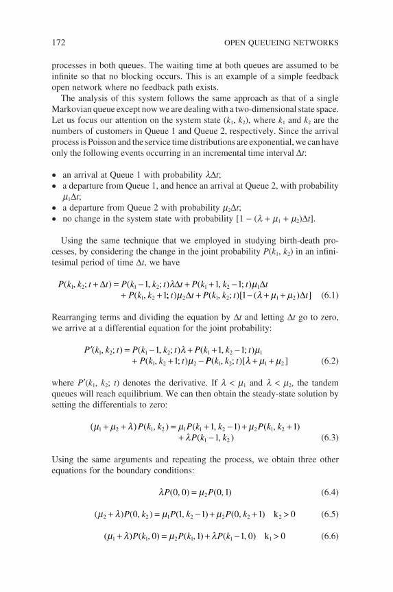
172 OPEN QUEUEING NETWORKS
processes in both queues. The waiting time at both queues are assumed to be infi nite so that no blocking occurs. This is an example of a simple feedback open network where no feedback path exists.
The analysis of this system follows the same approach as that of a single Markovian queue except now we are dealing with a two-dimensional state space. Let us focus our attention on the system state (k1, k2), where k1 and k2 are the numbers of customers in Queue 1 and Queue 2, respectively. Since the arrival process is Poisson and the service time distributions are exponential, we can have only the following events occurring in an incremental time interval ∆t:
• an arrival at Queue 1 with probability l∆t;
• a departure from Queue 1, and hence an arrival at Queue 2, with probability m1∆t;
• a departure from Queue 2 with probability m2∆t;
• no change in the system state with probability [1 − (l + m1 + m2)∆t].
Using the same technique that we employed in studying birth-death pro-cesses, by considering the change in the joint probability P(k1, k2) in an infi ni-tesimal period of time ∆t, we have
P k k t t P k k t t P k k t t
P k k( , ; ) ( , ; ) ( , ; )
( ,1 2 1 2 1 2 1
1 2
1 1 11
+ = − + + −+ +
∆ ∆ ∆λ µ;; ) ( , ; )[ ( ) ]t t P k k t tµ λ µ µ2 1 2 1 21∆ ∆+ − + + (6.1)
Rearranging terms and dividing the equation by ∆t and letting ∆t go to zero, we arrive at a differential equation for the joint probability:
′ = − + + −
+ + −P k k t P k k t P k k t
P k k t( , ; ) ( , ; ) ( , ; )
( , ; )1 2 1 2 1 2 1
1 2 2
1 1 11
λ µµ PP k k t( , ; )[ ]1 2 1 2λ µ µ+ + (6.2)
where P′(k1, k2; t) denotes the derivative. If l < m1 and l < m2, the tandem queues will reach equilibrium. We can then obtain the steady-state solution by setting the differentials to zero:
µ µ λ µ µ
λ1 2 1 2 1 1 2 2 1 2
1 2
1 1 11
+ +( ) = + − + ++ −
P k k P k k P k kP k k
( , ) ( , ) ( , )( , ) (6.3)
Using the same arguments and repeating the process, we obtain three other equations for the boundary conditions:
λ µP P( , ) ( , )0 0 0 12= (6.4)
( ) ( , ) ( , ) ( , )µ λ µ µ2 2 1 2 2 2 20 1 1 0 1 0+ = − + + >P k P k P k k (6.5)
( ) ( , ) ( , ) ( , )µ λ µ λ1 1 2 1 1 10 1 1 0 0+ = + − >P k P k P k k (6.6)
MARKOVIAN QUEUES IN TANDEM 173
Students will be quick to notice that this set of equations resembles that of the one-dimensional birth-death processes and can be interpreted as fl ow bal-ancing equations for probability fl ow going in and out of a particular state. The state transition diagram which refl ects this set of fl ow equations is shown in Figure 6.4.
Similar to the one-dimensional case, this set of equations is not independent of each other and the additional equation required for a unique solution is pro-vided by the normalization condition:
P k kkk
( , )1 2
21
1∑∑ = (6.7)
To solve Equations (6.3) to (6.6), let us assume that the solution has the so-called Product form, that is
P k k P k P k( , ) ( ) ( )1 2 1 1 2 2= (6.8)
where P1(k1) is the marginal probability function of Queue 1 and is a function of parameters of Queue 1 alone; similarly P2(k2) is the marginal probability function of Queue 2 and is a function of parameters of Queue 2 alone.
Substituting Equation (6.8) into Equation (6.4), we have
λ µP P2 2 20 1( ) ( )= (6.9)
Using it together with Equation (6.8) in Equation (6.6), we have
µ λ1 1 1 1 1 1P k P k( ) ( )= − (6.10)
P k P k
Pk
1 11
1 1
1 1 11
1
01
( ) ( )
( )
= −
= =
λµρ ρ λ
µwhere (6.11)
0,0 1,0
0,1
2,0
1,1
0,2
k1,0
k1–1,1
λ λ λ
λ
µ2µ2
µ2
µ1 µ1
µ1
λ
λ
µ2 µ2
Figure 6.4 State transition diagram of the tandem queues
174 OPEN QUEUEING NETWORKS
Since the marginal probability should sum to one, we have
P k P kk k
1 1 2 2
1 2
1 1∑ ∑= =( ) ( )and (6.12)
Using the expression (6.12), we obtain P1(0) = (1 − r1), therefore
P k k1 1 1 11 1( ) ( )= − ρ ρ (6.13)
Now, substituting Equations (6.10), (6.8) and (6.9) into Equation (6.3) and after simplifying terms, we arrive at
( ) ( ) ( ) ( )λ µ λ µ+ = − + +2 2 2 2 2 2 2 21 1P k P k P k (6.14)
This is a recursive equation in P2(k2), which we solve by z-transform:
P k z P k z P k zk
k
k
k
k2 2
12 2
12 2
12 2
2
2
2
2
2
1 1( )( ) ( ) ( )=
∞
=
∞
=
∞
∑ ∑ ∑+ = − + +λ µ λ µ kk2 (6.15)
Defi ne the z-transform of P2(k2) as
P z P k zk
k2 2 2
02
2( ) ( )==
∞
∑ (6.16)
We have from Equation (6.15):
( )[ ( ) ( )] ( ) ( ) ( ) ( )λ µ λ µ λµ
+ − = + − −
P z P zP zz
P z P P
P
2 2 22
2 22
2
2
0 0 0
(( )( )( ) ( )( )( )z z z P zρ ρ ρ λ µ2 2 2 2 21 1 0 1 1− − = + − =where /
and
P z Pz
2 22
2
01
1( ) ( )= +
−ρρ
(6.17)
Similarly, since the marginal probability P2 should sum to 1, that is equivalent to P2(z)|z=1 = 1, we arrive at
P22
2
01
1( ) = −
+ρρ
(6.18)
and
P zz
2 22
11
1( ) ( )= −
−ρ
ρ (6.19)
MARKOVIAN QUEUES IN TANDEM 175
Inverting the z-transform, we have
P k k2 2 2 21 2( ) ( )= − ρ ρ (6.20)
Therefore:
P k k k k( , ) ( ) ( )1 2 1 1 2 21 11 2= − −ρ ρ ρ ρ (6.21)
where ρ λµ
ρ λµ1
12
2
= =and
The expression of (6.21) holds for r0 < 1 and r1 < 1.For an isolated M/M/1 queueing system, the probability that there are k
customers in the system is P(k) = (1 − r)rk, therefore
P(k1, k2) = (1 − r1)r1k1(1 − r2)r2
k2
= P1(k1)P2(k2)
We see that the joint probability distribution is the product of the marginal probability distributions, and hence the term Product-Form solution.
6.1.1 Analysis of Tandem Queues
The foregoing analysis provides us with a steady-state solution but fails to give us an insight into the interaction between the two queues. The fi nal expression seems to suggest that the two queues are independent of each other. Are they really so?
To answer that, let us examine the two tandem queues in more detail. First let us look at Queue 1. The customer arriving pattern to Queue 1 is a Poisson process and the service times are distributed exponentially, therefore it is a classical M/M/1 queue.
How about Queue 2, what is the customer arriving pattern, or in other words the inter-arrival time distribution? It is clear from the connection diagram that the inter-departure time distribution from Queue 1 forms the inter-arrival time distribution of Queue 2. It can be shown that the customer arriving pattern to Queue 2 is a Poisson process as follows.
When a customer, say A, departs from Queue 1, he/she may leave behind an empty system with probability (1 − r1) or a busy system with probability r1. In the case of an empty system, the inter-departure time between A and the next customer (say B) is the sum of B’s service time and the inter-arrival time between A and B at Queue 1. Whereas in the busy system case, the inter-departure time is simply the service time of B.
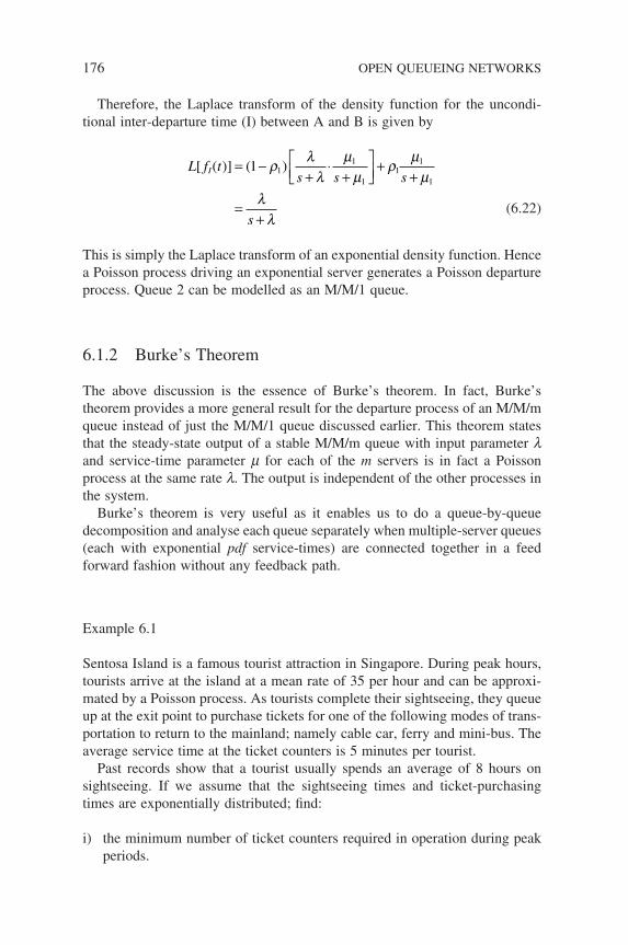
176 OPEN QUEUEING NETWORKS
Therefore, the Laplace transform of the density function for the uncondi-tional inter-departure time (I) between A and B is given by
L f t
s s s
s
I[ ( )] ( )= −+
⋅+
++
=+
1 11
11
1
1
ρ λλ
µµ
ρ µµ
λλ
(6.22)
This is simply the Laplace transform of an exponential density function. Hence a Poisson process driving an exponential server generates a Poisson departure process. Queue 2 can be modelled as an M/M/1 queue.
6.1.2 Burke’s Theorem
The above discussion is the essence of Burke’s theorem. In fact, Burke’s theorem provides a more general result for the departure process of an M/M/m queue instead of just the M/M/1 queue discussed earlier. This theorem states that the steady-state output of a stable M/M/m queue with input parameter l and service-time parameter m for each of the m servers is in fact a Poisson process at the same rate l. The output is independent of the other processes in the system.
Burke’s theorem is very useful as it enables us to do a queue-by-queue decomposition and analyse each queue separately when multiple-server queues (each with exponential pdf service-times) are connected together in a feed forward fashion without any feedback path.
Example 6.1
Sentosa Island is a famous tourist attraction in Singapore. During peak hours, tourists arrive at the island at a mean rate of 35 per hour and can be approxi-mated by a Poisson process. As tourists complete their sightseeing, they queue up at the exit point to purchase tickets for one of the following modes of trans-portation to return to the mainland; namely cable car, ferry and mini-bus. The average service time at the ticket counters is 5 minutes per tourist.
Past records show that a tourist usually spends an average of 8 hours on sightseeing. If we assume that the sightseeing times and ticket-purchasing times are exponentially distributed; fi nd:
i) the minimum number of ticket counters required in operation during peak periods.
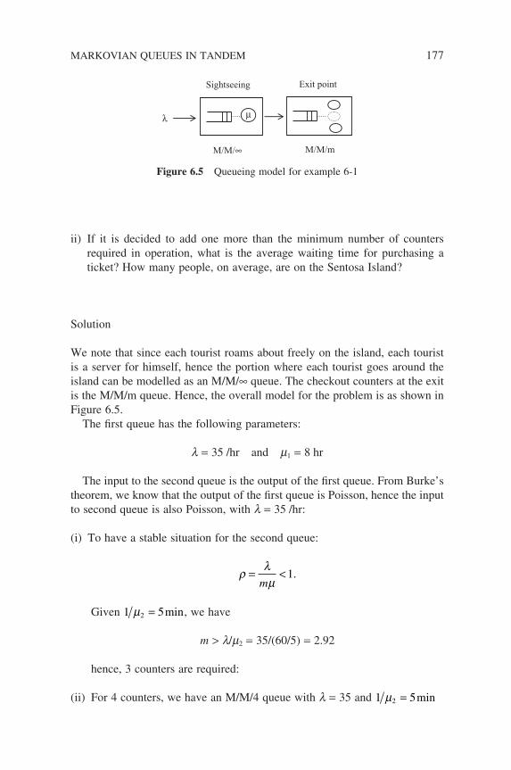
MARKOVIAN QUEUES IN TANDEM 177
ii) If it is decided to add one more than the minimum number of counters required in operation, what is the average waiting time for purchasing a ticket? How many people, on average, are on the Sentosa Island?
Solution
We note that since each tourist roams about freely on the island, each tourist is a server for himself, hence the portion where each tourist goes around the island can be modelled as an M/M/∞ queue. The checkout counters at the exit is the M/M/m queue. Hence, the overall model for the problem is as shown in Figure 6.5.
The fi rst queue has the following parameters:
l = 35 /hr and m1 = 8 hr
The input to the second queue is the output of the fi rst queue. From Burke’s theorem, we know that the output of the fi rst queue is Poisson, hence the input to second queue is also Poisson, with l = 35 /hr:
(i) To have a stable situation for the second queue:
ρ λµ
= <m
1.
Given 1 52µ = min, we have
m > l/m2 = 35/(60/5) = 2.92
hence, 3 counters are required:
(ii) For 4 counters, we have an M/M/4 queue with l = 35 and 1 52µ = min
M/M/∞ M/M/m
Sightseeing Exit point
µλ
Figure 6.5 Queueing model for example 6-1
178 OPEN QUEUEING NETWORKS
Pm
k
m
m
k
k
k
m m
k
00
1 1
1
1 35
12
35 12
= +−
=
+
=
− −
∑ ( )
!
( )
!( )
!
(
ρ ρρ
/ ))
!.
(
4
0
3
1
2 2
0
4 13548
0 0427
1
−( )
=
=−
=−
×
=
−
∑k
dWP
m m
P m
µ λ µ λρρ
ρ)
!( )
( )
!( )
. . min
m
m
P
hr
1
1
13
35 12
4 13 48
0 036 2 16
4
0
−
= ⋅
= =
/
/
and the average number of people waiting in line to purchase tickets Nq:
N Wq == ×=
λ35 0 036
1 26
( . )
.
N Nq22
1 99
= +
=
λµ
.
The total number of tourists (N) on the island is the sum of the number of tourists (N1) doing their sightseeing and the number of tourists (N2) at the exit point. It can be shown that the number of customers in an M/M/∞ is given by
N11
35
1 8
280
= =
=
λµ ( )/
Therefore N = N1 + N2
= 282
6.2 APPLICATIONS OF TANDEM QUEUES IN DATA NETWORKS
In a data network, messages (or packets) usually traverse from node to node across several links before they reach their destination. Superfi cially, this picture gives us an impression that the transmission of data packets across
several links can in a way be modelled as a cascade of queues in series. In reality, certain simplifying assumptions need to be made before the queueing results can be applied.
To understand the complications involved, we will consider two transmis-sion channels of same transmission speed in tandem in a packet switching network. This is a situation which is very similar to the queue in tandem that we discussed earlier. Unfortunately it warrants further consideration owing to the dependency between the two queues, as illustrated below:
(i) If packets have equal length, then the fi rst transmission channel can be modelled as an M/D/1 queue whereas the second transmission channel cannot be modelled as an M/D/1 queue because the departure process of the fi rst queue is no longer Poisson.
(ii) If packet lengths are exponentially distributed and are independent of each other as well as the inter-arrival times at the fi rst queue, the fi rst queue can be modelled as an M/M/1 queue but the second queue still cannot be modelled as an M/M/1 because the inter-arrival times are strongly corre-lated with the packet lengths and hence the service times. A packet that has a transmission time of t seconds at the fi rst channel will have the same transmission time at the second.
The second queue can be modelled as an M/M/1 only if the correlation is not present, i.e. a packet will assume a new exponential length upon departure from a transmission channel. Kleinrock (1975) suggested that merging several packet streams on a transmission channel has an effect similar to restoring the independence of inter-arrival times and packet lengths. This assumption is known as Kleinrock independence approximation.
With the Kleinrock’s approximation suggestion and coupled with Burke’s theorem, we are now in a position to estimate the average end-to-end delay of acyclic store-and-forward data networks. Virtual circuits in a packet switching network is a good example of a feed-forward queues in which packets traverse a virtual circuit from source to destination, as shown in Figure 6.6.
If we focus on a single virtual circuit then it generally has no feedback loop and can be approximately modelled as a series of queues, as shown in Figure 6.7.
The situation will not be so simple and straightforward when there are feed-back loops. The presence of feedback loops destroys the Poisson characteristic of the fl ow and Burke’s theorem will no longer be valid. We shall look at this type of network when we discuss Jackson’s queueing networks.
Referring to Figure 6.7, if we assume that packets of exponentially distrib-uted lengths arrive at Queue 1 according to a Poisson process and further assume that they take on new exponential lengths while traversing a cascade of queues in series, then the virtual circuit path can be decomposed into several M/M/1 queues and the average end-to-end delay for packets is then given by
APPLICATIONS OF TANDEM QUEUES IN DATA NETWORKS 179
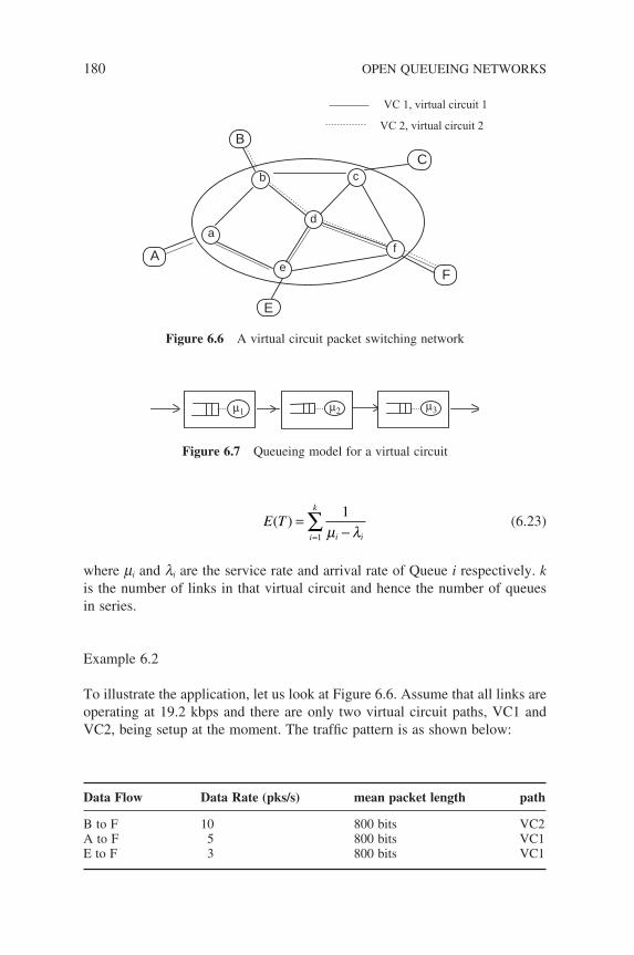
180 OPEN QUEUEING NETWORKS
E Ti ii
k
( ) =−=
∑ 1
1 µ λ (6.23)
where mi and li are the service rate and arrival rate of Queue i respectively. k is the number of links in that virtual circuit and hence the number of queues in series.
Example 6.2
To illustrate the application, let us look at Figure 6.6. Assume that all links are operating at 19.2 kbps and there are only two virtual circuit paths, VC1 and VC2, being setup at the moment. The traffi c pattern is as shown below:
VC 1, virtual circuit 1
VC 2, virtual circuit 2
E
B
F
C
A
a
b c
d
e
f
Figure 6.6 A virtual circuit packet switching network
µ1 µ2 µ3
Figure 6.7 Queueing model for a virtual circuit
Data Flow Data Rate (pks/s) mean packet length path
B to F 10 800 bits VC2A to F 5 800 bits VC1E to F 3 800 bits VC1
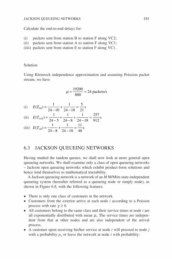
Calculate the end-to-end delays for:
(i) packets sent from station B to station F along VC2;(ii) packets sent from station A to station F along VC1;(iiii) packets sent from station E to station F along VC1.
Solution
Using Kleinrock independence approximation and assuming Poission packet stream, we have
µ = =19200
80024 packets/s
(i) E Tbdf( ) =−
+−
=1
24 10
1
24 18
5
21s
(ii) E Taedf( ) =−
+−
+−
=1
24 5
1
24 8
1
24 18
257
912s
(iii) E Tedf( ) =−
+−
=1
24 8
1
24 18
11
48s
6.3 JACKSON QUEUEING NETWORKS
Having studied the tandem queues, we shall now look at more general open queueing networks. We shall examine only a class of open queueing networks – Jackson open queueing networks which exhibit product-form solutions and hence lend themselves to mathematical tractability.
A Jackson queueing network is a network of an M M/M/m state-independent queueing system (hereafter referred as a queueing node or simply node), as shown in Figure 6.8, with the following features:
• There is only one class of customers in the network.
• Customers from the exterior arrive at each node i according to a Poisson process with rate gi ≥ 0.
• All customers belong to the same class and their service times at node i are all exponentially distributed with mean mi. The service times are indepen-dent from that at other nodes and are also independent of the arrival process.
• A customer upon receiving his/her service at node i will proceed to node j with a probability pij or leave the network at node i with probability:
JACKSON QUEUEING NETWORKS 181
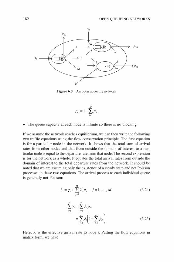
182 OPEN QUEUEING NETWORKS
p pio ijj
M
= −=
∑11
.
• The queue capacity at each node is infi nite so there is no blocking.
If we assume the network reaches equilibrium, we can then write the following two traffi c equations using the fl ow conservation principle. The fi rst equation is for a particular node in the network. It shows that the total sum of arrival rates from other nodes and that from outside the domain of interest to a par-ticular node is equal to the departure rate from that node. The second expression is for the network as a whole. It equates the total arrival rates from outside the domain of interest to the total departure rates from the network. It should be noted that we are assuming only the existence of a steady state and not Poisson processes in these two equations. The arrival process to each individual queue is generally not Poisson:
λ γ λi i j jij
M
p j M= + ==
∑1
1, . . . , (6.24)
γ λ
λ
ii
M
i ioi
M
ii
M
ijj
M
p
p
= =
= =
∑ ∑
∑ ∑
=
= −
1 1
1 1
1 (6.25)
Here, li is the effective arrival rate to node i. Putting the fl ow equations in matrix form, we have
p10
γ1
γ3
γ2
p30
p20
1
i
µ
µ
µM
Figure 6.8 An open queueing network
λ λ γi j jij
M
ip i M− = ==
∑1
1 2, , . . . , (6.26)
I P
I P
T
T
λ λ γ
λ γ
− =
− =( ) (6.27)
where
I
TM
TM
is the identity matrix
λ λ λ λ
γ γ γ γ
=
=
[ , , . . . , ]
[ , , . . . , ]
1 2
1 2
PP
p p p
p p
p p
M
M MM
=
11 12 1
21 22
1
. . .
. . .
. . . . . . . . . . . .
(6.28)
Jackson demonstrated in 1957 (Jackson 1957) that the joint probability dis-tribution for this type of network exhibits the product-form solution. i.e.:
P n P n n n
P n P n P nM
M M
( ) ( , , . . . , )
( ) ( ) . . . ( )
==
1 2
1 1 2 2 (6.29)
where Pi(ni) is the marginal probability distribution of each node i.We present here a simple verifi cation of the product-form solution assuming
that all nodes are in an M/M/1 queue. In fact, the Jackson’s result is applicable to multi-server and state dependent cases. To begin with, we defi ne the follow-ing notations:
ñ = (n1, n2, . . . , ni, . . . , nM)
1i = (0, 0, . . . , 1, 0, 0)
ñ − 1i = (n1, n2, . . . , ni − 1, . . . , nM)
ñ + 1i = (n1, n2, . . . , ni + 1, . . . , nM)
Parallel to the analysis of tandem queues, we again focus our attention on the change in system state ñ in an incremental time interval ∆t. The system as a whole is Markov because the arrival processes are all Poisson and service processes are exponential, therefore there can only be four types of transition, as follows:
JACKSON QUEUEING NETWORKS 183
184 OPEN QUEUEING NETWORKS
• no change in system state
• an arrival to node i
• a departure from node i
• transfer of a customer from node i to node j.
The corresponding transitional probability for the network going from state m to state ñ due to the above mentioned four events is
P n m
t t m n
t m n
p
ii
M
ii
M
i i
i ijj
M( )
=
− − =
= +
−
= =
=
∑ ∑1
1
1
1 1
1
γ µ
γ
µ
∆ ∆
∆
∑∑
= −
= + −
∆
∆
t m n
p t m n
i
i ij j i
1
1 1µ
Therefore
P n t t P n t t t
P n t
ii
M
ii
M
[ ( )] [ ( )]
[ ( )
+ = − −
+ −
= =∑ ∑∆ ∆ ∆1
1
1 1
γ µ
ii ii
M
i i ijj
M
i
M
t P n t p t
P n t
] [ ( ) ]
[ ( )
γ µ∆ ∆= ==∑ ∑∑+ + −
+
1 11
1 1
++ −==
∑∑ 1 111
j i j jij
M
i
M
p t]µ ∆
(6.30)
Rearranging terms, dividing the equation by ∆t, taking limit and dropping the time parameter, we have
d
dtP n P n P n
P n
ii
M
ii
M
i ii
M
( ) ( ) ( )
(
= − −
+ −
+
= = =∑ ∑ ∑γ µ γ
1 1 1
1
++ −
+ + −== ==
∑∑ ∑∑ 1 1 1 111 11
i i ijj
M
i
M
j jij
M
i
M
j ip p P n) ( )µ µ
(6.31)
Setting the derivative of the joint probability density function to zero, we obtain
γ µ γ µii
M
ii
M
i ii
M
i ijj
M
P n P n p= = = =∑ ∑ ∑ ∑+
= − + −1 1 1 1
1 1( ) ( )
+
+ − +
=
==
∑
∑∑
P n
p P n
ii
M
j ji i jj
M
i
M
( )
( )
1
1 1
1
11
µ
(6.32)
This is a rather complex equation to deal with, so instead of solving the equation directly we do the reverse. With a bit of hindsight, let us suggest that the fi nal solution P(ñ) satisfi es the following relationships:
P n P ni i( ) ( ) − = −1 1ρ (6.33)
P n P ni i( ) ( ) + =1 ρ (6.34)
P n P ni j i j( ) ( ) − + = −1 1 1ρ ρ (6.35)
where as usual rk = lk/mk. The validity of this suggestion can be verifi ed by showing that they indeed satisfy the general fl ow balance Equation (6.32). Substituting them into Equation (6.32), we have
γ µ γ ρ µ ρ µii
M
ii
M
i ii
M
i ijj
M
i
M
i j jp p= =
−
= ==∑ ∑ ∑ ∑∑+ = + −
+1 1
1
1 11
1 ii i jj
M
i
M
ρ ρ−
==∑∑ 1
11
So far we have not used the fl ow conservation Equations (6.24) and (6.25). The above equation can be further simplifi ed by using these two equations. In doing so, we arrive at
γ µ λ λ ρ γ λii
M
ii
M
i j jij
M
ii
M
ii
M
j jip p= = =
−
= =∑ ∑ ∑∑ ∑+ = −
+ +1 1 1
1
1 1
ρρ
µ γ
ij
M
i
M
ii
M
ii
M
−
==
= =
∑∑
∑ ∑= +
1
11
1 1
(6.36)
Now, we have established the validity of our suggested relationships of P(ñ), it is easy for us to fi nd the fi nal expression of P(ñ) using expression (6.33):
P n P n
P n n n n
P n n
i i
i i M
ini
( ) ( )
( , , . . . , , . . . , )
( , , .
= −= −=
ρρρ
1
11 2
1 2 .. . , , . . . , )
( , , . . . , )
( )
0
0 0 0
0
1
1
n
P
P
M
in
i
M
in
i
M
i
i
=
=
=
=
∏
∏
ρ
ρ
(6.37)
JACKSON QUEUEING NETWORKS 185
186 OPEN QUEUEING NETWORKS
The P(0) can be found, as usual, by the normalization condition:
P n P
P
P
nin
i
M
n
in
ni
M
i
i
i
( ) ( )
( )
(
∑ ∏∑
∑∏
=
=
=
=
=
∞
=
0 1
0 1
1
01
ρ
ρ
0 1 1
0 1
1
1
1
) ( )
( ) ( )
− =
= −
=
−
=
∏
∏
ρ
ρ
ii
M
ii
M
P
(6.38)
Hence, the fi nal solution is given by
P n
P n P n P n
ii
M
in
M M
i( ) ( )
( ) ( ) . . . . ( )
= −
==
∏ 11
1 1 2 2
ρ ρ
(6.39)
The condition for stability in the network is li/mi < 1 and we shall assume that this condition exists throughout all our discussions.
There are two observations we can derive from the about expression. Firstly, the expression seems to suggest that each queue in the network behaves as if it is independent of the others and hence the joint state probability is a product of the marginal probabilities. Secondly, each queue can be considered sepa-rately in isolation, even though the arrival is not Poisson due to the feedback paths.
6.3.1 Performance Measures for Open Networks
Jackson’s theorem coupled with Little’s theorem provides us with a simple means of evaluating some of the performance parameters of an open queueing network:
(i) Total throughput of the network g. This follows from the fl ow conservation principle, as the total number of
customers entering the system should be the same as the total number of customers leaving the system, if it is stable.
γ γ= ∑ ii
(6.40)
(ii) The average number of times a customer visits a node Vi is
Vi i= λ γ/ (6.41)
and the network-wide average number of times a customer visits a typical node V is
V ii
= ∑λ γ (6.42)
(iii) The marginal probability of node i is, in general, defi ned as
P k P n n ni Mn ki
( ) ( , , . . . , )==
∑ 1 2 (6.43)
Subject to the normalization condition
P n( ) .∑ = 1
(iv) Once the marginal probability is obtained, the marginal queue length for the ith node in theory can be calculated. For a product-form open queueing network consisting of only single-server queues, the marginal queue length is the same as that of an isolated M/M/1, as shown below. The arrival rate li (or load) to each node can be obtained from the overall traffi c pattern using fl ow conservation Equations (6.24) and (6.25):
nii
ii
i
i
=−
=ρ
ρρ λ
µ1and (6.44)
Then the total number of customers in the whole system (network) is
N n n nM
i
ii
M
i
i ii
M
= + + +
=−
=−
=
=
∑
∑
1 2
1
1
1
1
. . . .
ρρ
λµ λ
(all M/M/ queues) (6.45)
(v) Average time spent in the network:
TN
ii
M
ii
Mi
i ii
M
= =−
= =
=∑ ∑∑
γ γ
λµ λ
1 1
1
1 (6.46)
JACKSON QUEUEING NETWORKS 187
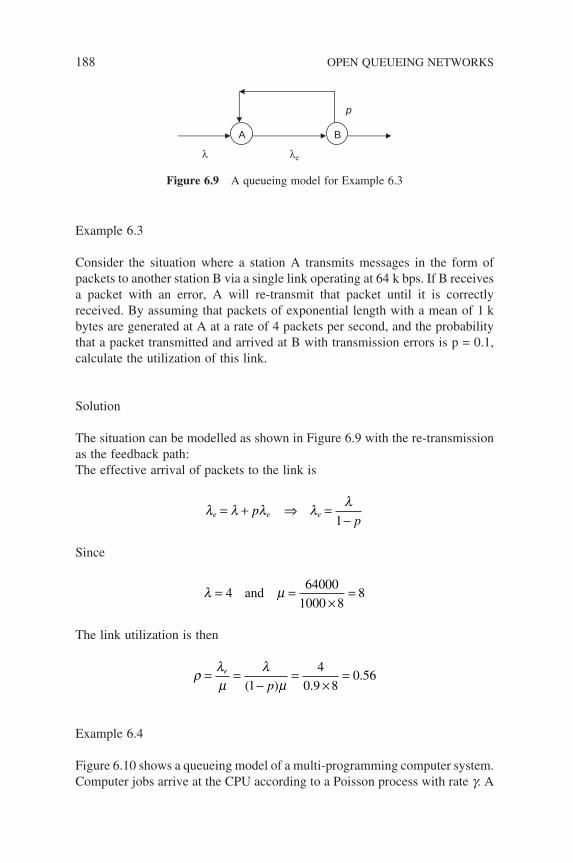
188 OPEN QUEUEING NETWORKS
Example 6.3
Consider the situation where a station A transmits messages in the form of packets to another station B via a single link operating at 64 k bps. If B receives a packet with an error, A will re-transmit that packet until it is correctly received. By assuming that packets of exponential length with a mean of 1 k bytes are generated at A at a rate of 4 packets per second, and the probability that a packet transmitted and arrived at B with transmission errors is p = 0.1, calculate the utilization of this link.
Solution
The situation can be modelled as shown in Figure 6.9 with the re-transmission as the feedback path:The effective arrival of packets to the link is
λ λ λ λ λe e ep
p= + ⇒ =
−1
Since
λ µ= =×
=464000
1000 88and
The link utilization is then
ρ λµ
λµ
= =−
=×
=e
p( ) ..
1
4
0 9 80 56
Example 6.4
Figure 6.10 shows a queueing model of a multi-programming computer system. Computer jobs arrive at the CPU according to a Poisson process with rate g. A
A B
p
λ λe
Figure 6.9 A queueing model for Example 6.3
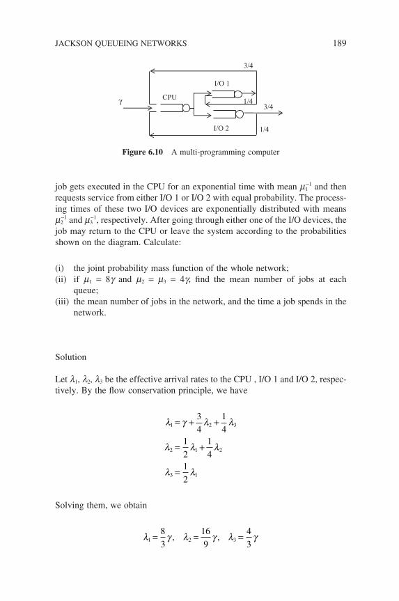
job gets executed in the CPU for an exponential time with mean m1−1 and then
requests service from either I/O 1 or I/O 2 with equal probability. The process-ing times of these two I/O devices are exponentially distributed with means m2
−1 and m3−1, respectively. After going through either one of the I/O devices, the
job may return to the CPU or leave the system according to the probabilities shown on the diagram. Calculate:
(i) the joint probability mass function of the whole network;(ii) if m1 = 8g and m2 = m3 = 4g, fi nd the mean number of jobs at each
queue;(iii) the mean number of jobs in the network, and the time a job spends in the
network.
Solution
Let l1, l2, l3 be the effective arrival rates to the CPU , I/O 1 and I/O 2, respec-tively. By the fl ow conservation principle, we have
λ γ λ λ
λ λ λ
λ λ
1 2 3
2 1 2
3 1
3
4
1
41
2
1
41
2
= + +
= +
=
Solving them, we obtain
λ γ λ γ λ γ1 2 38
3
16
9
4
3= = =, ,
I/O 2
I/O 1
CPUγ 1/4
3/4
1/4
3/4
Figure 6.10 A multi-programming computer
JACKSON QUEUEING NETWORKS 189
190 OPEN QUEUEING NETWORKS
(i) The joint probability mass function is then given by Jackson’s theorem:
P n n n( , , )1 2 31 2 3 1
18
31
16
91
4
3
8
3= −
−
−
γµ
γµ
γµ
γµ
n n n1 2 316
9
4
32 3
γµ
γµ
(ii) ρ λµ
ρ ρ11
12 3
1
3
4
9
1
3= = = =, ,
NCPU =
−=
−=ρ
ρ1
11
1 3
1 1 3
1
2
/
/( )
N NI O I O/ /and1 2
4
5
1
2= =
(iii) N N N NCPu I O I O= + + =/ /1 29
5
T = =9 5 9
5
/
γ γ
6.3.2 Balance Equations
Students who are familiar with the probability fl ow balance concept discussed earlier will be able to recognize that Equation (6.32) is the network version of the global balance equation encountered in Chapter 4. The equation basically equates the total probability fl ow in and out of the state ñ.
The left-hand side of the equation is the probability fl ow leaving state ñ due to arrivals or departure from the queues. The fi rst term on the right corresponds to the probability fl ow from state (ñ − 1i) into state ñ due to an arrival, the second term is the probability fl ow from state (ñ + 1i) into state ñ due to a departure and the last term is the probability fl ow from (ñ − 1i + 1j) into state ñ due to a transfer of a customer from node i to j.
The expressions (6.33) to (6.35) are simply the local balance equations. These local balance equations must satisfy the global balance equation. It should be noted that the local balance concept is a unique property peculiar to product-form queueing networks. It is a stronger and more stringent form of balance than global balance. A solution that satisfi es all the local balance equa-tions also satisfi es the global balance equations, but the converse does not necessary hold.
Example 6.5
Consider the virtual-circuit packet-switching network shown in Figure 6.6, and the traffi c load together with the routing information as given in Table 6.1. If
all the links operate at 9600 bps and the average length of a packet is 320 bits, calculate:
(i) The network-wide packet delay;(ii) The average number of hops a packet will traverse through the network.
Solution
(i) The network-wide delay is given by the expression
T
ii
Mi
i ii
M
=−
=
=∑∑1
1
1γ
λµ λ
Let us calculate the last summation using the data listed in Table 6.2. Since the transmission speed is the same for all links:
mi = 9600/320 = 30
The total load to each link (li) can be obtained from Table 6.1. For example, Link 1 (ab) has a total load of 4(ab) + 1(abc) + 3(eab) = 8 and Link 4 (ea) has a total traffi c load of 1 (ea) + 3 (eab) + 10 (fea) = 14.Once:
λµ λ
i
i ii
M
−=
=∑
1
5 5499.
is calculated, it remains for us to calculate the sum of total external arrival
rates to the network γ ii
M
=∑
1
. This can be obtained by assuming packets
Table 6.1 Traffi c load and routing information
a b c e f
a — 4 (ab) 1 (abc) 3 (ae) 6 (aef)b 5 (ba) — 4 (bc) 1 (bde) 10 (bdf)c 2 (cba) 2 (cb) — 1 (cde) 3 (cf)e 1 (ea) 3 (eab) 7 (edc) — 1 (ef)f 10 (fea) 1 (fdb) 2 (fc) 4 (fe) —
* The number in each cell indicates the mean number of packets per second that are transmitted from a source (row) to a destina-tion (column). The alphabet string indicates the path taken by these packets.
JACKSON QUEUEING NETWORKS 191
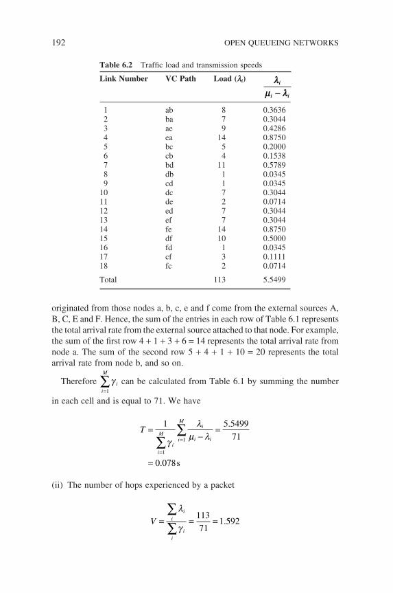
192 OPEN QUEUEING NETWORKS
originated from those nodes a, b, c, e and f come from the external sources A, B, C, E and F. Hence, the sum of the entries in each row of Table 6.1 represents the total arrival rate from the external source attached to that node. For example, the sum of the fi rst row 4 + 1 + 3 + 6 = 14 represents the total arrival rate from node a. The sum of the second row 5 + 4 + 1 + 10 = 20 represents the total arrival rate from node b, and so on.
Therefore γ ii
M
=∑
1
can be calculated from Table 6.1 by summing the number
in each cell and is equal to 71. We have
T
ii
Mi
i ii
M
=−
=
==
=∑∑1 5 5499
71
0 0781
1γ
λµ λ
.
. s
(ii) The number of hops experienced by a packet
Vi
i
ii
= = =∑∑
λ
γ113
711 592.
Table 6.2 Traffi c load and transmission speeds
Link Number
VC Path
Load (li)
lm l
i
i i-
1 ab 8 0.3636 2 ba 7 0.3044 3 ae 9 0.4286 4 ea 14 0.8750 5 bc 5 0.2000 6 cb 4 0.1538 7 bd 11 0.5789 8 db 1 0.0345 9 cd 1 0.034510 dc 7 0.304411 de 2 0.071412 ed 7 0.304413 ef 7 0.304414 fe 14 0.875015 df 10 0.500016 fd 1 0.034517 cf 3 0.111118 fc 2 0.0714
Total 113 5.5499
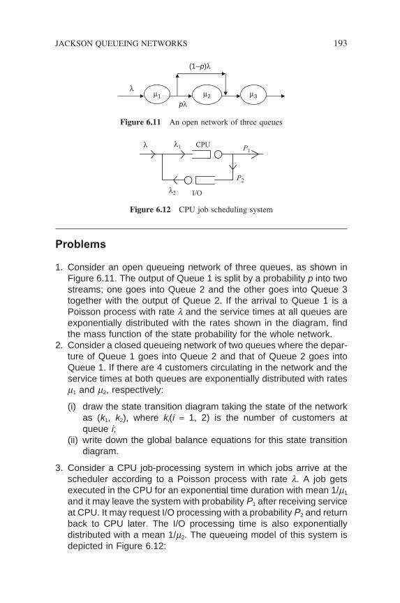
Problems
1. Consider an open queueing network of three queues, as shown in Figure 6.11. The output of Queue 1 is split by a probability p into two streams; one goes into Queue 2 and the other goes into Queue 3 together with the output of Queue 2. If the arrival to Queue 1 is a Poisson process with rate l and the service times at all queues are exponentially distributed with the rates shown in the diagram, fi nd the mass function of the state probability for the whole network.
2. Consider a closed queueing network of two queues where the depar-ture of Queue 1 goes into Queue 2 and that of Queue 2 goes into Queue 1. If there are 4 customers circulating in the network and the service times at both queues are exponentially distributed with rates m1 and m2, respectively:
(i) draw the state transition diagram taking the state of the network as (k1, k2), where ki(i = 1, 2) is the number of customers at queue i;
(ii) write down the global balance equations for this state transition diagram.
3. Consider a CPU job-processing system in which jobs arrive at the scheduler according to a Poisson process with rate l. A job gets executed in the CPU for an exponential time duration with mean 1/m1 and it may leave the system with probability P1 after receiving service at CPU. It may request I/O processing with a probability P2 and return back to CPU later. The I/O processing time is also exponentially distributed with a mean 1/m2. The queueing model of this system is depicted in Figure 6.12:
µ1λ
(1–p)λ
pλµ2 µ3
Figure 6.11 An open network of three queues
CPU
I/O
P1
P2
λ λ1
λ2
Figure 6.12 CPU job scheduling system
JACKSON QUEUEING NETWORKS 193
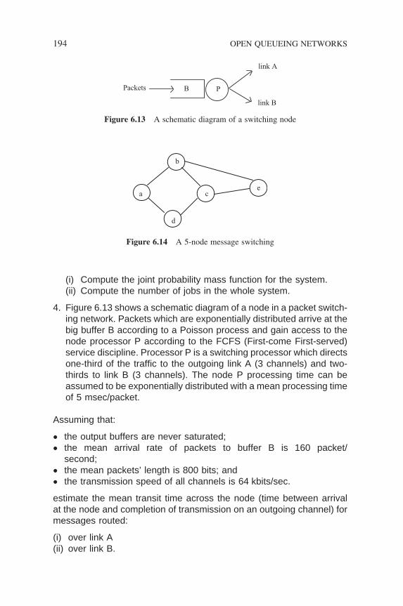
194 OPEN QUEUEING NETWORKS
(i) Compute the joint probability mass function for the system.(ii) Compute the number of jobs in the whole system.
4. Figure 6.13 shows a schematic diagram of a node in a packet switch-ing network. Packets which are exponentially distributed arrive at the big buffer B according to a Poisson process and gain access to the node processor P according to the FCFS (First-come First-served) service discipline. Processor P is a switching processor which directs one-third of the traffi c to the outgoing link A (3 channels) and two-thirds to link B (3 channels). The node P processing time can be assumed to be exponentially distributed with a mean processing time of 5 msec/packet.
Assuming that:
• the output buffers are never saturated;• the mean arrival rate of packets to buffer B is 160 packet/
second;• the mean packets’ length is 800 bits; and• the transmission speed of all channels is 64 kbits/sec.
estimate the mean transit time across the node (time between arrival at the node and completion of transmission on an outgoing channel) for messages routed:
(i) over link A(ii) over link B.
Packets
link A
link B
B P
Figure 6.13 A schematic diagram of a switching node
a
b
d
ce
Figure 6.14 A 5-node message switching
5. Consider the message-switching network shown in Figure 6.14, and the traffi c load together with the routing information as shown in Table 6.3. If all links operate at 19.2 kbps and the average length of a message is 960 bits, calculate:
(i) the network-wide message delay; and(ii) the average delay experience by a message traversing the path
adce.
Table 6.3 Traffi c load and routing information for Figure 6.14
a b c d e
a — 5 (ab) 7 (adc) 1 (ab) 3 (abc)b 2 (ba) — 3 (bc) 1 (bcd) 5 (bc)c 3 (cba) 4 (cb) — 4 (cd) 10 (ce)d 10 (da) 5 (dcb) 3 (dc) — 1 (dce)e 5 (ecda) 2 (eb) 4 (ec) 1 (ecd) —
JACKSON QUEUEING NETWORKS 195

7Closed Queueing Networks
In this chapter, we shall complete our analysis of queueing networks by looking at another class that has neither external arrivals nor departures – closed queue-ing networks. As before, we shall restrict our discussion to where all customers in the networks have the same service demand distribution. These types of networks are often termed as single customer class (or single class) networks in contrast to multi-class networks in which customers belong to different classes and each class has its own service demand distribution. Students should not confuse these multi-class networks with priority queueing systems. In multi-class queueing networks, customers of different classes are treated equally and selected for service according to the prevailing queueing discipline, even though they have different service-time distributions.
Closed queueing networks are often more useful than their open counterparts because the infi nite customer population assumption that is implicit in open queueing networks is unrealistic. Many interesting problems in computer and communication networks can be formulated as closed queueing networks.
7.1 JACKSON CLOSED QUEUEING NETWORKS
For simplicity, we shall deal only with a class of closed queueing networks that parallel the Jackson open queueing networks. The structure of a Jackson closed network is similar to that of the open network. It is a closed queueing network of M queues with N customers circulating in the network with the following characteristics:
Queueing Modelling Fundamentals Second Edition Ng Chee-Hock and Soong Boon-Hee© 2008 John Wiley & Sons, Ltd
198 CLOSED QUEUEING NETWORKS
• All customers have the same service demand distribution. They are served in their order of arrivals at node i and their service demands are exponen-tially distributed with an average rate mi, which is independent of other processes in the network.
• A customer completing service at node i will proceed to node j with a prob-ability of pij.
• There is no blocking at each node, in other words, the capacity of each node is greater than or equal to (N − 1).
The equilibrium state distribution is given by the joint probability vector:
P(ñ) ≡ P(n1, n2, . . . , nM)
Since there are no external arrivals or departures in a closed queueing network, by setting pio = 0 and gi = 0 in Equation (6.24), we obtain the following traffi c equations:
piji
M
==∑ 1
1
(7.1)
λ λi j jij
M
p==
∑1
(7.2)
Equation (7.2) is a set of homogeneous linear equations that has no unique solution. Any solution e = (e1, e2, . . . , eM) or its multiplier ke is also a solution. Here we use the new notation ei instead of li because li is no longer the absolute arrival rate to Queue i and the ratio (li/mi) is also not the actual utilization (ri) of Queue i.
To solve this equation, we can set one of the ei s to a certain convenient value, such as 1. If we set e1 = 1, then ei(i > 1) can be interpreted as the mean number of visits by a customer to node i(i > 1) relative to the number of visits to station 1, which is also 1. Therefore, ei is sometimes called the relative visi-tation rate of Queue i.
The state space (S) of a closed queueing network is fi nite since there are a fi xed number of customers circulating in the system. The state space (S) is
S n n n n n NM i ii
M
= ≥ =
=
∑( , , . . . ) &1 21
0 (7.3)
Using the method shown in Example 1.2, the number of states in S will be
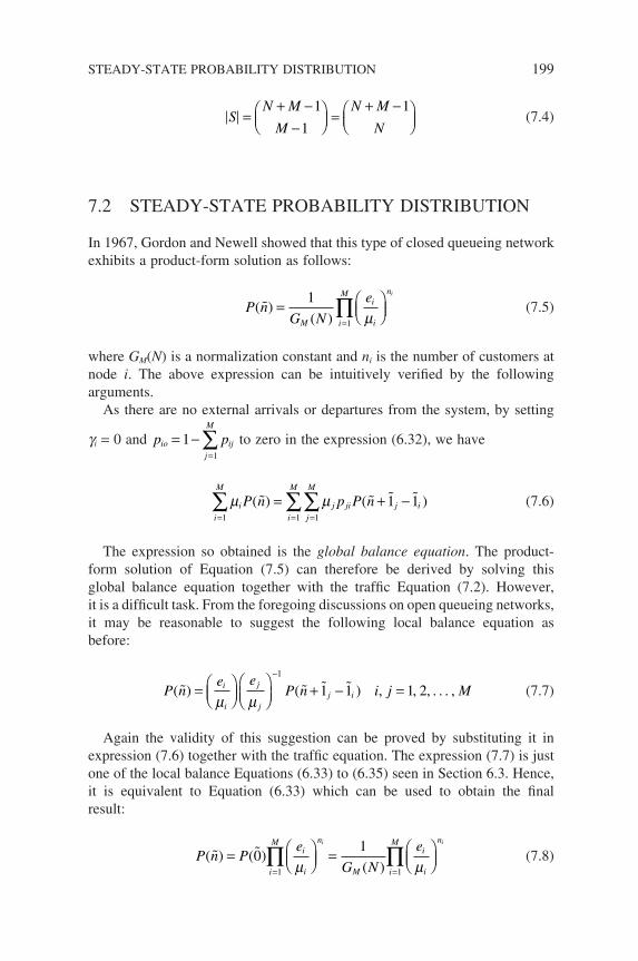
SN M
M
N M
N=
+ −−
=
+ −
1
1
1 (7.4)
7.2 STEADY-STATE PROBABILITY DISTRIBUTION
In 1967, Gordon and Newell showed that this type of closed queueing network exhibits a product-form solution as follows:
P nG N
e
M
i
i
n
i
M i
( )( )
=
=
∏1
1 µ (7.5)
where GM(N) is a normalization constant and ni is the number of customers at node i. The above expression can be intuitively verifi ed by the following arguments.
As there are no external arrivals or departures from the system, by setting
gi = 0 and p pio ijj
M
= −=
∑11
to zero in the expression (6.32), we have
µ µii
M
j ji j ij
M
i
M
P n p P n( ) ( ) = ==∑ ∑∑= + −
1 11
1 1 (7.6)
The expression so obtained is the global balance equation. The product-form solution of Equation (7.5) can therefore be derived by solving this global balance equation together with the traffi c Equation (7.2). However, it is a diffi cult task. From the foregoing discussions on open queueing networks, it may be reasonable to suggest the following local balance equation as before:
P ne e
P n i j Mi
i
j
jj i( ) ( ) , , , . . . , =
+ − =−
µ µ
1
1 1 1 2 (7.7)
Again the validity of this suggestion can be proved by substituting it in expression (7.6) together with the traffi c equation. The expression (7.7) is just one of the local balance Equations (6.33) to (6.35) seen in Section 6.3. Hence, it is equivalent to Equation (6.33) which can be used to obtain the fi nal result:
P n Pe
G N
ei
i
n
Mi
Mi
i
n
i
Mi i
( ) ( )( )
=
=
= =
∏ ∏01
1 1µ µ (7.8)
STEADY-STATE PROBABILITY DISTRIBUTION 199
200 CLOSED QUEUEING NETWORKS
The normalization constant GM(N) is used in the expression instead of P(0) to signify that it can be evaluated recursively, as we shall show in the next section. By defi nition, it is given by the usual normalization of probability
P nn S
( )
=⊂∑ 1 , i.e.:
G Ne
Mi
i
n
i
M
n S
i
( ) =
=⊂
∏∑ µ1
(7.9)
It is clear from the above that GM(N) is a function of both the number of queues (M) and the total number of customers (N) in the network. Students should also realize that it is also a function of ei’s,mi’s and pij’s, although they are not explicitly expressed in the notation.
Once the normalization constant is calculated, we can then calculate the performance measures. Since there is neither external arrival nor departure from the network, certain performance measures for opening networks are not applicable here, such as the throughput of the network.
The marginal probability of node i is the probability that node i contains exactly ni = k customers. It is the sum of the probabilities of all possible
states that satisfi es n Nii
M
==∑
1
and ni = k; i.e.:
P k P n n ni M
n N n ki i
( ) ( , , . . . , )&
=∑ = =
∑ 1 2 (7.10)
Again, subject to the normalization condition:
P n( ) . =∑ 1
Interestingly, we shall see in the next section that most of the statistical parameters of interest for a closed queueing network can be obtained in terms of GM(N) without the explicit evaluation of P(ñ).
Example 7.1
Consider a closed queueing network, as shown in Figure 7.1, with two custom-ers circulating in the network. Customers leaving Queue 2 and Queue 3 will automatically join back to Queue 1 for service. If service times at the three queues are exponentially distributed with rate m and the branching probability at the output of Queue 1 is p = 0.5, fi nd the joint probability distribution and other performance measures for the network.
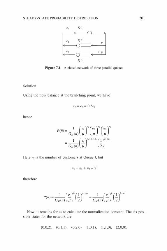
Solution
Using the fl ow balance at the branching point, we have
e2 = e3 = 0.5e1
hence
P nG n
e e e
G n
e
M
n n n
M
( )( )
( )
=
=
1
1
1 2 3
1
1 2 3
µ µ µ
µ
+ + +n n n n n1 2 3 2 31
2
Here ni is the number of customers at Queue I, but
n1 + n2 + n3 = 2
therefore
P nG n
e
G n
e
M
n n
M
( )( ) ( )
=
=
+ −1 1
2
1 1
21
21
2 22 3
µ µ
nn1
Now, it remains for us to calculate the normalization constant. The six pos-sible states for the network are
(0,0,2), (0,1,1), (0,2,0) (1,0,1), (1,1,0), (2,0,0).
Q 2
Q 3
Q 1
p
1–p
e1
e2
e3
Figure 7.1 A closed network of three parallel queues
STEADY-STATE PROBABILITY DISTRIBUTION 201
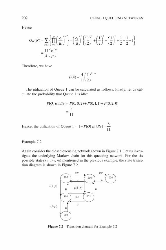
202 CLOSED QUEUEING NETWORKS
Hence
G Ne e
Mi
i
n
i
M i
( ) =
=
+
+
=∏ µ µ1
12 2 21
2
1
2
1
2
+ + +
=
⊂∑
2
12
1
2
1
21
11
4
n S
e
µ
Therefore, we have
P nn
( ) =
−4
11
1
2
2 1
The utilization of Queue 1 can be calculated as follows. Firstly, let us cal-culate the probability that Queue 1 is idle:
P Q is idle P P P[ ] ( , , ) ( , , ) ( , , )1 0 0 2 0 1 1 0 2 0
3
11
= + +
=
Hence, the utilization of Queue 1 = 1 18
11− =P Q is idle[ ]
Example 7.2
Again consider the closed queueing network shown in Figure 7.1. Let us inves-tigate the underlying Markov chain for this queueing network. For the six possible states (n1, n2, n3) mentioned in the previous example, the state transi-tion diagram is shown in Figure 7.2.
µ(1–p) µ(1–p)
µ p
µ p
µ p
µ
µ
µµ
µ
µ
µ(1–p)
002
101 011
110200 020
Figure 7.2 Transition diagram for Example 7.2
CONVOLUTION ALGORITHM 203
Writing the global balance equation for each state using the notation of P(n1 n2 n3) for state probability, we have
(200) mP(200) = mP(110) + mP(101)(110) 2mP(110) = mP(020) + mP(011) + 0.5 mP(200)(020) mP(020) = 0.5 mP(110)(101) 2 mP(101) = 0.5 mP(200) + mP(011) + mP(002)(011) 2 mP(011) = 0.5 mP(110) + 0.5 mP(101)(002) mP(002) = 0.5 mP(101)
The normalization condition is
P(110) + P(011) + P(200) + P(020) + P(002) + P(101) = 1
Solving this set of equations, we have
P P P
P P P
( ) , ( ) , ( )
( ) , ( ) , (
0021
11101
2
11011
1
11
1102
11200
4
1102
= = =
= = 001
11) =
The utilization for Queue 1:
ρ1 110 200 101
2
11
4
11
2
11
8
11
= + +
= + + =
P P P( ) ( ) ( )
7.3 CONVOLUTION ALGORITHM
Before we proceed to evaluate performance measures of a closed queueing network using P(ñ), as we did in the case of a single queueing system, let us examine the problem faced with calculating GM(N), which is part of the expres-sion of P(ñ). As pointed out earlier, the state space for a closed queueing network with M queues and N customers is given by
SN M
M
N M
N=
+ −−
=
+ −
1
1
1 (7.11)
So for a network with moderate M and N, it is rather computationally expen-sive to evaluate GM(N) and often the process will quickly run into the usual combinatorial problem. In the 1970s, Buzen developed an effi cient recursive algorithm for computing the normalization constants (Buzen 1973). This
204 CLOSED QUEUEING NETWORKS
somehow reduces the computational burden of evaluating performance mea-sures for a closed queueing network. However, the computation is still sub-stantial, as we shall see later. Here we describe the so-called convolution algorithm, which is due to (Buzen 1973), for the case where queues in the network are not state-dependent, that is, we have constant mi.
Recall that
G Ne
Mi
i
n
i
M
n S
i
( ) =
=∈
∏∑ µ1
(7.12)
If we defi ne a function g(n,m) similar to GM(N) in defi nition, we use the lower case n and m to signify that gm(n) can later be expressed as a recursive function in terms of gm−1(n) and gm(n − 1). By considering the case when the last queue (M) is empty and when it has customers, it can be shown that
g n g ne
g nm mm
mm( ) ( ) ( )= +
−−1 1
µ (7.13)
This is a convolution-like recursive expression enabling us to compute gm(n) progressively using the following initial conditions:
g n e n Nn1 1 1 1 2( ) ( / ) , , . . . ,= =µ (7.14)
g m Mm ( ) , , . . . ,0 1 1 2= = (7.15)
Example 7.3
Consider a closed queueing network of three parallel queues, as shown in Figure 7.3. The service times at all three queues are exponentially distributed with mean m−1 and the branching probability p = 1/2.
Q 2
Q 3
Q 1
p
1–p
e1
e2
e3
Figure 7.3 A closed network of three parallel queues
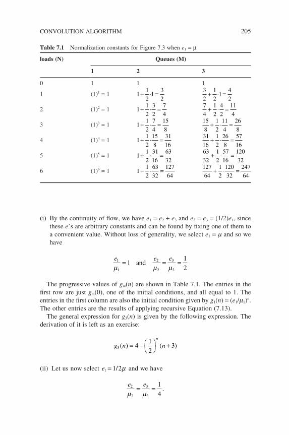
CONVOLUTION ALGORITHM 205
(i) By the continuity of fl ow, we have e1 = e2 + e3 and e2 = e3 = (1/2)e1, since these e’s are arbitrary constants and can be found by fi xing one of them to a convenient value. Without loss of generality, we select e1 = m and so we have
e e e1
1
2
2
3
3
11
2µ µ µ= = =and
The progressive values of gm(n) are shown in Table 7.1. The entries in the fi rst row are just gm(0), one of the initial conditions, and all equal to 1. The entries in the fi rst column are also the initial condition given by g1(n) = (e1/m1)n. The other entries are the results of applying recursive Equation (7.13).
The general expression for g3(n) is given by the following expression. The derivation of it is left as an exercise:
g n nn
3 41
23( ) ( )= −
+
(ii) Let us now select e1 1 2= / µ and we have
e e2
2
3
3
1
4µ µ= = .
Table 7.1 Normalization constants for Figure 7.3 when e1 = µ
loads (N) Queues (M)
1 2 3
0 1 1 1
1 (1)1 = 1 11
21
3
2+ ⋅ =
3
2
1
21
4
2+ ⋅ =
2 (1)2 = 1 11
2
3
2
7
4+ ⋅ =
7
4
1
2
4
2
11
4+ ⋅ =
3 (1)3 = 1 11
2
7
4
15
8+ ⋅ =
15
8
1
2
11
4
26
8+ ⋅ =
4 (1)4 = 1 11
2
15
8
31
16+ ⋅ =
31
16
1
2
26
8
57
16+ ⋅ =
5 (1)5 = 1 11
2
31
16
63
32+ ⋅ =
63
32
1
2
57
16
120
32+ ⋅ =
6 (1)6 = 1 11
2
63
32
127
64+ ⋅ =
127
64
1
2
120
32
247
64+ ⋅ =
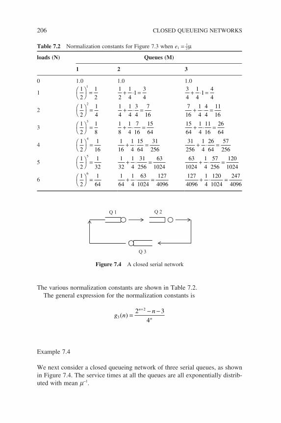
206 CLOSED QUEUEING NETWORKS
The various normalization constants are shown in Table 7.2.The general expression for the normalization constants is
g nnn
n3
22 3
4( ) =
− −+
Example 7.4
We next consider a closed queueing network of three serial queues, as shown in Figure 7.4. The service times at all the queues are all exponentially distrib-uted with mean m−1.
Table 7.2 Normalization constants for Figure 7.3 when e1 = 1–2 µ
loads (N) Queues (M)
1 2 3
0 1.0 1.0 1.0
11
2
1
2
1
=
1
2
1
41
3
4+ ⋅ =
3
4
1
41
4
4+ ⋅ =
21
2
1
4
2
=
1
4
1
4
3
4
7
16+ ⋅ =
7
16
1
4
4
4
11
16+ ⋅ =
31
2
1
8
3
=
1
8
1
4
7
16
15
64+ ⋅ =
15
64
1
4
11
16
26
64+ ⋅ =
41
2
1
16
4
=
1
16
1
4
15
64
31
256+ ⋅ =
31
256
1
4
26
64
57
256+ ⋅ =
51
2
1
32
5
=
1
32
1
4
31
256
63
1024+ ⋅ =
63
1024
1
4
57
256
120
1024+ ⋅ =
61
2
1
64
6
=
1
64
1
4
63
1024
127
4096+ ⋅ =
127
4096
1
4
120
1024
247
4096+ ⋅ =
Q 1 Q 2
Q 3
Figure 7.4 A closed serial network
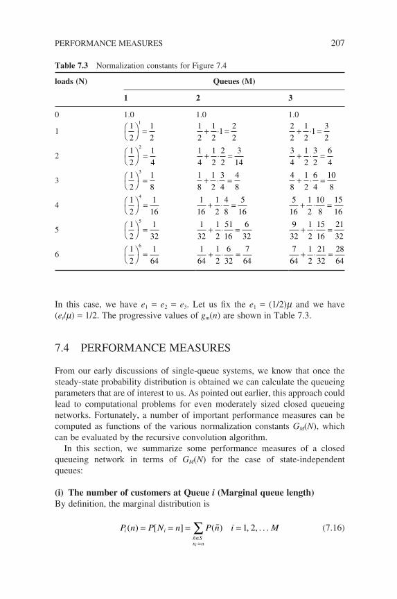
In this case, we have e1 = e2 = e3. Let us fi x the e1 = (1/2)m and we have (ei/m) = 1/2. The progressive values of gm(n) are shown in Table 7.3.
7.4 PERFORMANCE MEASURES
From our early discussions of single-queue systems, we know that once the steady-state probability distribution is obtained we can calculate the queueing parameters that are of interest to us. As pointed out earlier, this approach could lead to computational problems for even moderately sized closed queueing networks. Fortunately, a number of important performance measures can be computed as functions of the various normalization constants GM(N), which can be evaluated by the recursive convolution algorithm.
In this section, we summarize some performance measures of a closed queueing network in terms of GM(N) for the case of state-independent queues:
(i) The number of customers at Queue i (Marginal queue length)By defi nition, the marginal distribution is
P n P N n P n i Mi in Sn ni
( ) [ ] ( ) , , . . .= = = =∈=
∑
1 2 (7.16)
Table 7.3 Normalization constants for Figure 7.4
loads (N) Queues (M)
1 2 3
0 1.0 1.0 1.0
11
2
1
2
1
=
1
2
1
21
2
2+ ⋅ =
2
2
1
21
3
2+ ⋅ =
21
2
1
4
2
=
1
4
1
2
2
2
3
14+ ⋅ =
3
4
1
2
3
2
6
4+ ⋅ =
31
2
1
8
3
=
1
8
1
2
3
4
4
8+ ⋅ =
4
8
1
2
6
4
10
8+ ⋅ =
41
2
1
16
4
=
1
16
1
2
4
8
5
16+ ⋅ =
5
16
1
2
10
8
15
16+ ⋅ =
51
2
1
32
5
=
1
32
1
2
51
16
6
32+ ⋅ =
9
32
1
2
15
16
21
32+ ⋅ =
61
2
1
64
6
=
1
64
1
2
6
32
7
64+ ⋅ =
7
64
1
2
21
32
28
64+ ⋅ =
PERFORMANCE MEASURES 207
208 CLOSED QUEUEING NETWORKS
From Chapter 1 Equation (1.8), we see that Pi(n) can also be computed as
P n P N n P N ni i i( ) [ ] [ ]= ≥ − ≥ +1 (7.17)
However
P N n P ng N
ei
n Sn n
M
j
j
n
j
M
n Sn ni
j
i
[ ] ( )( )
≥ = =
∈
≥=∈
≥
∑ ∏∑
1
1 µ (7.18)
Since Queue i has more than n customers, we can factor out (ei/mi)n from the last product term, and what remains is simply the normalization constant with N − n customers. Hence
P N ne g N n
g Ni
i
i
nM
M
[ ]( )
( )≥ =
−µ
(7.19)
Substituting back into Equation (7.17), we have
P ne
g Ng N n
eg N ni
i
i
n
MM
i
iM( )
( )( ) ( )=
− −
− −
µ µ
11 (7.20)
(ii) The mean number of customers at Queue iThe mean number of customers at Queue i is by defi nition
E N kP N ki ik
N
[ ] [ ]= ==
∑1
(7.21)
But from Example 1.8 in Chapter 1, we know that the expected value of a dis-crete random variable can alternatively be computed as
E N P N k
e g N k
g N
i ik
N
i
i
kM
Mk
N
[ ] [ ]
( )
( )
= ≥
=
−=
=
∑
∑1
1 µ
(7.22)
(iii) Marginal utilization of node iFor a single-server queueing network, the marginal utilization of node i is
ρ
µ
i i i
i
i
M
M
P N P N
e g N
g N
= − = = ≥
=
−1 0 1
1
[ ] [ ]
( )
( )
(7.23)
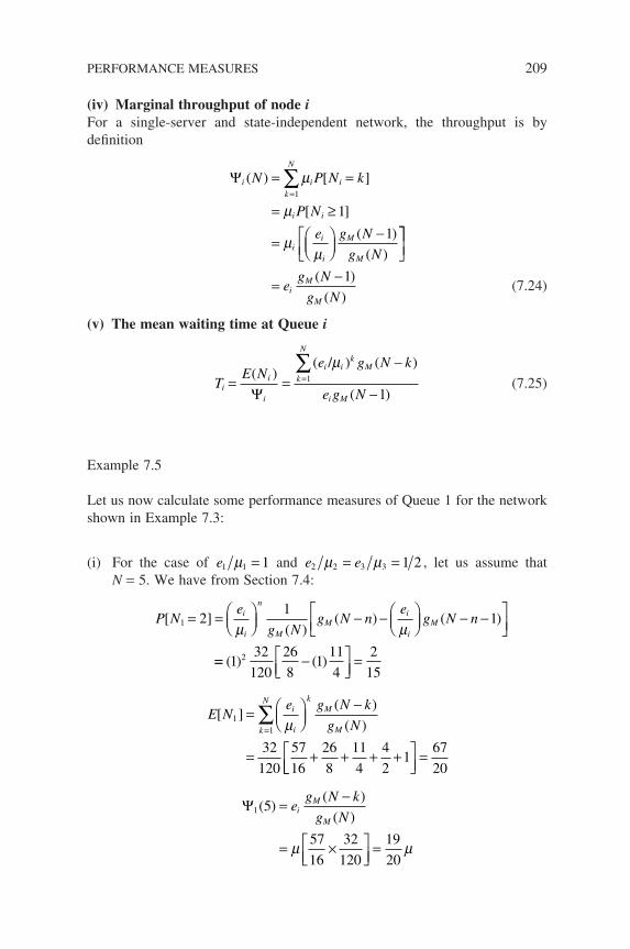
(iv) Marginal throughput of node iFor a single-server and state-independent network, the throughput is by defi nition
Ψi i ik
N
i i
ii
i
M
M
N P N k
P N
e g N
g N
( ) [ ]
[ ]
( )
( )
= =
= ≥
=
−
=∑µ
µ
µµ
1
1
1
=−
eg N
g Ni
M
M
( )
( )
1
(7.24)
(v) The mean waiting time at Queue i
TE N
e g N k
e g Ni
i
i
i ik
Mk
N
i M
= =−
−=
∑( )( / ) ( )
( )Ψ
µ1
1 (7.25)
Example 7.5
Let us now calculate some performance measures of Queue 1 for the network shown in Example 7.3:
(i) For the case of e1 1 1µ = and e e2 2 3 3 1 2µ µ= = , let us assume that N = 5. We have from Section 7.4:
P Ne
g Ng N n
eg N ni
i
n
MM
i
iM[ ]
( )( ) ( )1 2
11= =
− −
− −
µ µ
== −
=( ) ( )132
120
26
81
11
4
2
152
E Ne g N k
g Ni
i
kM
Mk
N
[ ]( )
( )1
1
32
120
57
16
26
8
11
4
4
21
=
−
= + + + +=
∑ µ
=67
20
Ψ1 5
57
16
32
120
19
20
( )( )
( )=
−
= ×
=
eg N k
g Ni
M
M
µ µ
PERFORMANCE MEASURES 209
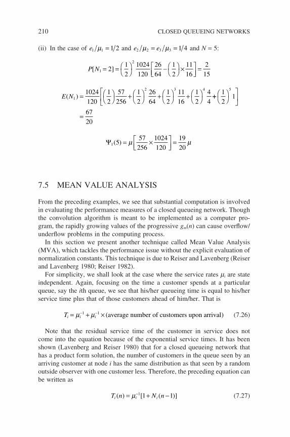
210 CLOSED QUEUEING NETWORKS
(ii) In the case of e1 1 1 2µ = and e e2 2 3 3 1 4µ µ= = and N = 5:
P N[ ]1
2
21
2
1024
120
26
64
1
2
11
16
2
15= =
−
×
=
E N( )1
2 3 41024
120
1
2
57
256
1
2
26
64
1
2
11
16
1
2
4
4=
+
+
+
++
=
1
21
67
20
5
Ψ1 557
256
1024
120
19
20( ) = ×
=µ µ
7.5 MEAN VALUE ANALYSIS
From the preceding examples, we see that substantial computation is involved in evaluating the performance measures of a closed queueing network. Though the convolution algorithm is meant to be implemented as a computer pro-gram, the rapidly growing values of the progressive gm(n) can cause overfl ow/underfl ow problems in the computing process.
In this section we present another technique called Mean Value Analysis (MVA), which tackles the performance issue without the explicit evaluation of normalization constants. This technique is due to Reiser and Lavenberg (Reiser and Lavenberg 1980; Reiser 1982).
For simplicity, we shall look at the case where the service rates mi are state independent. Again, focusing on the time a customer spends at a particular queue, say the ith queue, we see that his/her queueing time is equal to his/her service time plus that of those customers ahead of him/her. That is
Ti i i= + ×− −µ µ1 1 ( )average number of customers upon arrival (7.26)
Note that the residual service time of the customer in service does not come into the equation because of the exponential service times. It has been shown (Lavenberg and Reiser 1980) that for a closed queueing network that has a product form solution, the number of customers in the queue seen by an arriving customer at node i has the same distribution as that seen by a random outside observer with one customer less. Therefore, the preceding equation can be written as
T n N ni i i( ) [ ( )]= + −−µ 1 1 1 (7.27)
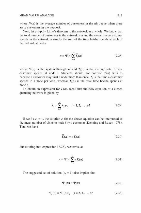
where Ni(n) is the average number of customers in the ith queue when there are n customers in the network.
Now, let us apply Little’s theorem to the network as a whole. We know that the total number of customers in the network is n and the mean time a customer spends in the network is simply the sum of the time he/she spends at each of the individual nodes:
n n T nii
M
==∑Ψ( ) ( )
1
(7.28)
where Ψ(n) is the system throughput and Ti(n) is the average total time a customer spends at node i. Students should not confuse Ti(n) with Ti because a customer may visit a node more than once. Ti is the time a customer spends in a node per visit, whereas Ti(n) is the total time he/she spends at node i.
To obtain an expression for Ti(n), recall that the fl ow equation of a closed queueing network is given by
λ λi j jij
M
p i M= ==
∑1
1 2, , . . . , (7.29)
If we fi x e1 = 1, the solution ei for the above equation can be interpreted as the mean number of visits to node i by a customer (Denning and Buxen 1978). Thus we have
T n e T ni i i( ) ( )= (7.30)
Substituting into expression (7.28), we arrive at
n n e T ni ii
M
==∑Ψ( ) ( )
1
(7.31)
The suggested set of solution (e1 = 1) also implies that
Ψ Ψ1( ) ( )n n= (7.32)
Ψ Ψj jn n e j M( ) ( ) , , . . . ,= =1 2 3 (7.33)
MEAN VALUE ANALYSIS 211
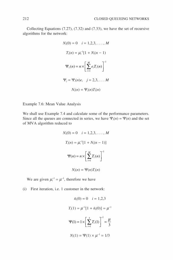
212 CLOSED QUEUEING NETWORKS
Collecting Equations (7.27), (7.32) and (7.33), we have the set of recursive algorithms for the network:
Ni(0) = 0 i = 1,2,3, . . . , M
Ti(n) = mi−1[1 + Ni(n − 1)
Ψ11
1
( ) ( )n n e T ni ii
M
= ×
=
−
∑
Ψj = Ψi(n)ei j = 2,3, . . . M
Ni(n) = Ψi(n)Ti(n)
Example 7.6: Mean Value Analysis
We shall use Example 7.4 and calculate some of the performance parameters. Since all the queues are connected in series, we have Ψi(n) = Ψ(n) and the set of MVA algorithm reduced to
Ni(0) = 0 i = 1,2,3, . . . , M
Ti(n) = mi−1[1 + Ni(n − 1)]
Ψ( ) ( )n n T nii
M
= ×
=
−
∑1
1
Ni(n) = Ψ(n)Ti(n)
We are given mi−1 = m−1, therefore we have
(i) First iteration, i.e. 1 customer in the network:
ni(0) = 0 i = 1,2,3
Ti(1) = m−1[1 + ni(0)] = m−1
Ψ( ) ( )1 1 131
3 1
= ×
==
−
∑Tii
µ
Ni(1) = Ψ(1) × m−1 = 1/3
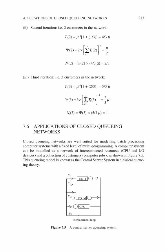
(ii) Second iteration: i.e. 2 customers in the network:
Ti(2) = m−1[1 + (1/3)] = 4/3 m
Ψ( ) ( )2 2 221
3 1
= ×
==
−
∑Tii
µ
Ni(2) = Ψ(2) × (4/3 m) = 2/3
(iii) Third iteration: i.e. 3 customers in the network:
Ti(3) = m−1[1 + (2/3)] = 5/3 m
Ψ( ) ( )3 3 33
51
3 1
= ×
==
−
∑Tii
µ
Ni(3) = Ψ(3) × (5/3 m) = 1
7.6 APPLICATIONS OF CLOSED QUEUEING NETWORKS
Closed queueing networks are well suited for modelling batch processing computer systems with a fi xed level of multi-programming. A computer system can be modelled as a network of interconnected resources (CPU and I/O devices) and a collection of customers (computer jobs), as shown in Figure 7.5. This queueing model is known as the Central Server System in classical queue-ing theory.
CPU
I/O M
I/O 1 p1
p2
p0
pM
Replacement loop
Figure 7.5 A central server queueing system
APPLICATIONS OF CLOSED QUEUEING NETWORKS 213
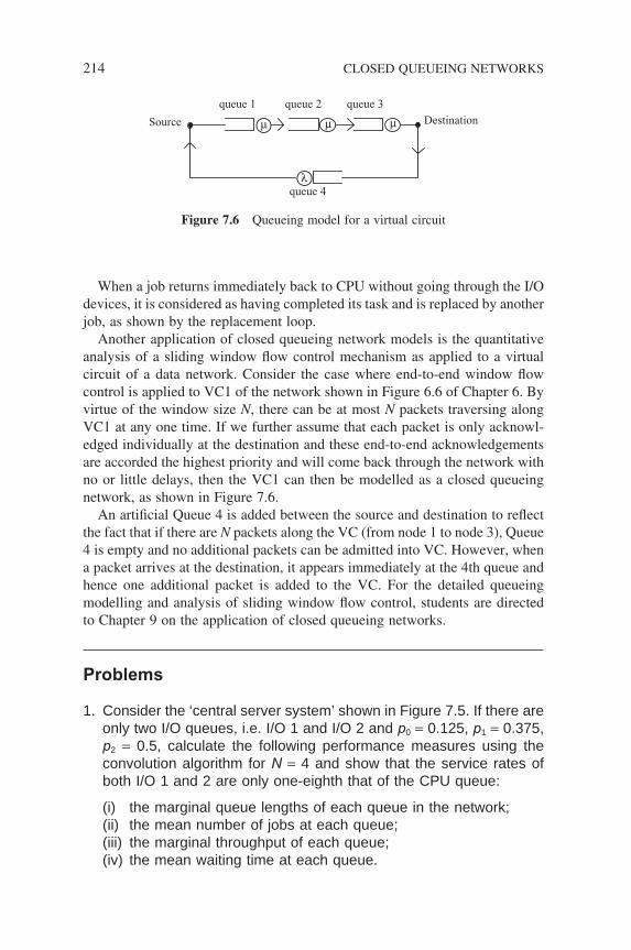
214 CLOSED QUEUEING NETWORKS
When a job returns immediately back to CPU without going through the I/O devices, it is considered as having completed its task and is replaced by another job, as shown by the replacement loop.
Another application of closed queueing network models is the quantitative analysis of a sliding window fl ow control mechanism as applied to a virtual circuit of a data network. Consider the case where end-to-end window fl ow control is applied to VC1 of the network shown in Figure 6.6 of Chapter 6. By virtue of the window size N, there can be at most N packets traversing along VC1 at any one time. If we further assume that each packet is only acknowl-edged individually at the destination and these end-to-end acknowledgements are accorded the highest priority and will come back through the network with no or little delays, then the VC1 can then be modelled as a closed queueing network, as shown in Figure 7.6.
An artifi cial Queue 4 is added between the source and destination to refl ect the fact that if there are N packets along the VC (from node 1 to node 3), Queue 4 is empty and no additional packets can be admitted into VC. However, when a packet arrives at the destination, it appears immediately at the 4th queue and hence one additional packet is added to the VC. For the detailed queueing modelling and analysis of sliding window fl ow control, students are directed to Chapter 9 on the application of closed queueing networks.
Problems
1. Consider the ‘central server system’ shown in Figure 7.5. If there are only two I/O queues, i.e. I/O 1 and I/O 2 and p0 = 0.125, p1 = 0.375, p2 = 0.5, calculate the following performance measures using the convolution algorithm for N = 4 and show that the service rates of both I/O 1 and 2 are only one-eighth that of the CPU queue:
(i) the marginal queue lengths of each queue in the network;(ii) the mean number of jobs at each queue;(iii) the marginal throughput of each queue;(iv) the mean waiting time at each queue.
queue 1 queue 2 queue 3
queue 4 λ
µ µ µSource Destination
Figure 7.6 Queueing model for a virtual circuit
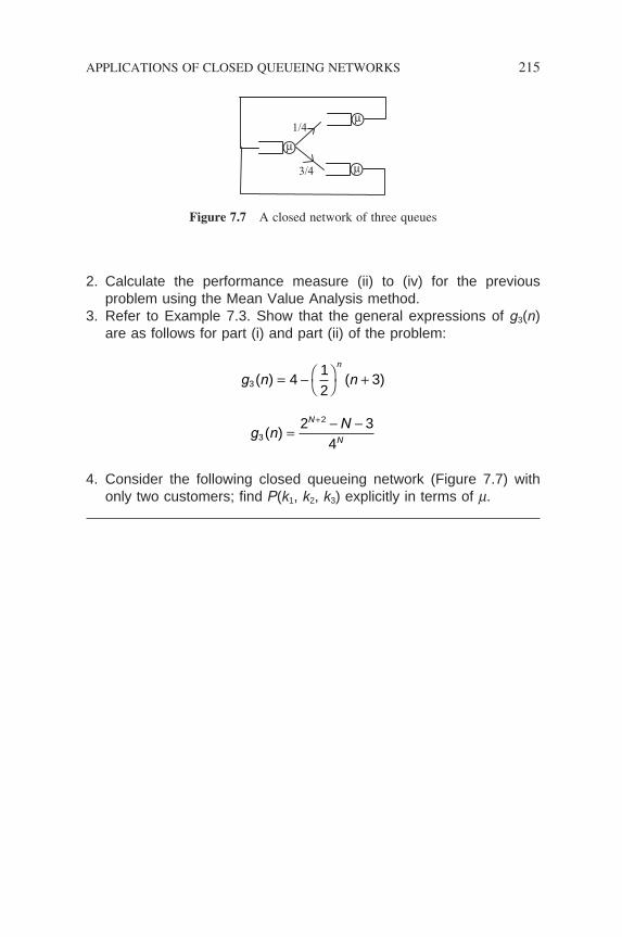
2. Calculate the performance measure (ii) to (iv) for the previous problem using the Mean Value Analysis method.
3. Refer to Example 7.3. Show that the general expressions of g3(n) are as follows for part (i) and part (ii) of the problem:
g n nn
3 41
23( ) ( )= −
+
g nNN
N3
22 3
4( ) =
− −+
4. Consider the following closed queueing network (Figure 7.7) with only two customers; fi nd P(k1, k2, k3) explicitly in terms of m.
µ
µ
µ
1/4
3/4
Figure 7.7 A closed network of three queues
APPLICATIONS OF CLOSED QUEUEING NETWORKS 215

8Markov-Modulated Arrival Process
In all the queueing systems (or networks) that we have discussed so far, we have always adopted the rather simple arrival model – Poisson or General Independent process that specifi cally assumes arrivals occur independently of one another and of the service process. This simple assumption is not always adequate in modelling real-life data traffi c, which exhibits correlations in their arrivals, especially the new services found in Asynchronous Transfer Mode (ATM) or broadband networks.
ATM is a transport mechanism recommended for the Broadband Integrated Services Digital Network that is supposedly capable of handling a wide mixture of traffi c sources; ranging from the traditional computer data, to packetized voice and motion video. In this multi-media traffi c, the arrival instants are in some sense correlated and exhibit a diverse mixture of traffi c characteristics with different correlations and burstiness. As queueing system performances are highly sensitive to these correlations and bursty characteristics in the arrival process, we need more realistic models to represent the arrival process.
In this chapter, we fi rst examine three traffi c models, namely:
• Markov-modulated Poisson Process (MMPP)
• Markov-modulated Bernoulli process (MMBP), and
• Markov-modulated Fluid Flow.
These traffi c models are widely used as source models in performance evalua-tion of multi-media traffi c due to their ability to capture the strong correlation
Queueing Modelling Fundamentals Second Edition Ng Chee-Hock and Soong Boon-Hee© 2008 John Wiley & Sons, Ltd
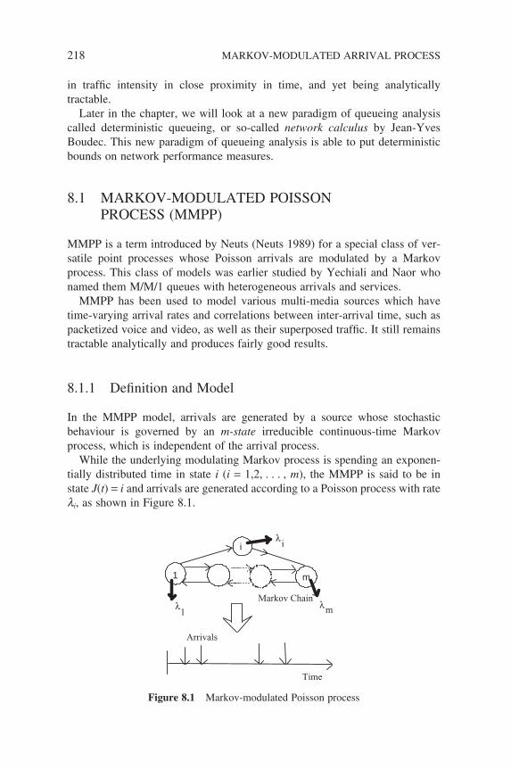
218 MARKOV-MODULATED ARRIVAL PROCESS
in traffi c intensity in close proximity in time, and yet being analytically tractable.
Later in the chapter, we will look at a new paradigm of queueing analysis called deterministic queueing, or so-called network calculus by Jean-Yves Boudec. This new paradigm of queueing analysis is able to put deterministic bounds on network performance measures.
8.1 MARKOV-MODULATED POISSON PROCESS (MMPP)
MMPP is a term introduced by Neuts (Neuts 1989) for a special class of ver-satile point processes whose Poisson arrivals are modulated by a Markov process. This class of models was earlier studied by Yechiali and Naor who named them M/M/1 queues with heterogeneous arrivals and services.
MMPP has been used to model various multi-media sources which have time-varying arrival rates and correlations between inter-arrival time, such as packetized voice and video, as well as their superposed traffi c. It still remains tractable analytically and produces fairly good results.
8.1.1 Defi nition and Model
In the MMPP model, arrivals are generated by a source whose stochastic behaviour is governed by an m-state irreducible continuous-time Markov process, which is independent of the arrival process.
While the underlying modulating Markov process is spending an exponen-tially distributed time in state i (i = 1,2, . . . , m), the MMPP is said to be in state J(t) = i and arrivals are generated according to a Poisson process with rate li, as shown in Figure 8.1.
1
i
m
Time
Arrivals
Markov Chainλ
λ
λ1 m
i
Figure 8.1 Markov-modulated Poisson process
The Markov-modulated Poisson process (MMPP) is a doubly stochastic Poisson process whose rate varies according to a continuous time function. In this case, the time function is the underlying Markov chain. MMPP is fully characterized by the following parameters:
(i) The transition-rate matrix (also known as the infi nitesimal generator Q) of the underlying modulating Markov process:
Q
q q q
q q q
q q
m
m
m m
=
−−
−
1 12 1
21 2 2
1
(8.1)
where
q qi ijjj i
m
==≠
∑1
We assume here that the transition-rate matrix Q is homogeneous, i.e. Q does not vary with time. The steady-state vector:
π = [p1, p2, . . . , pm]
of the modulating Markov chain is then given by
π Q = 0 and p1 + p2 + . . . + pm = 1
(ii) The Poisson arrival rate at each state l1, l2, . . . , lm. We defi ne a diagonal matrix Λ and a vector λ as
Λ =
=
diag m
m
( , , . . . )λ λ λλ
λ
λ
1 2
1
2
0 0
0 0
0
0 0
(8.2)
λ λ λ λ= ( , , . . . )1 2 mT (8.3)
MARKOV-MODULATED POISSON PROCESS (MMPP) 219
220 MARKOV-MODULATED ARRIVAL PROCESS
(iii) The initial state (initial probability vector) of the MMPP, i.e.:
ϕ ϕi ii
P J t i= = = =∑[ ( ) ] & .0 1
Depending on the initial vector chosen, we have
(a) an interval-stationary MMPP that starts at an ‘arbitrary’ arrival epoch if the initial vector is chosen as
ϕπ λ π λ π λ
π=+ + +
1
1 1 2 2 . . . m m
Λ (8.4)
(b) an environment stationary MMPP whose initial probability vector is chosen as π, which is the stationary vector of Q . Now the origin of time is not an arrival epoch, but is chosen so that the environmental Markov process is stationary.
Having described the model, let us examine the distribution of the inter-arrival time of an MMPP. If we denote Xk as the time between (k − 1) arrival and k arrival, and Jk the state of the underlying Markov process at the time of the kth arrival, then the sequence (Jk,Xk), k ≥ 0 is a Markov renewal sequence with a transition probability distribution matrix given by
F x e d
e Q
I e
Qx
Q x
( )
[ ( ) ]
[( ) ]
( )
(
=
= − −
= −
−
− −
∫ Λ
Λ
Λ
Λ Λ
ς
ς
ς0
10
QQ x Q− −− Λ Λ Λ) ( ) 1 (8.5)
The elements Fij(x) of the matrix are the conditional probabilities:
F x P J j X x J iij k k k( ) , = = ≤ =−1 (8.6)
The transition probability density matrix is then given by differentiating F(x) with respect to x:
f xd
dxF x e Q Q
e
Q x
Q x
( ) ( ) ( )( )( )
( )
= = − − −
=
− − −
−
Λ
Λ
Λ Λ Λ
Λ
1
(8.7)
Taking the Laplace transform of f (x), we have
L f x e e dx
sI Q e
Q x sx
sI Q
[ ( )]
[ ( )
( )
( )
=
= − − +
− −∞
− − − +
∫ Λ
Λ
Λ
Λ0
1 xx
sI Q
]
( )
0
1
∞
−= − +
Λ
Λ Λ (8.8)
Now let us consider N(t), the number of arrivals in (0, t). If J(t) is the state of the Markov process at time t, defi ne a matrix P(n, t) whose (i, j) entry is
P n t P N t n J t j N t J t iij ( , ) [ ( ) , ( ) ( ) , ( ) ]= = = = = = =0 0 0 (8.9)
Then the matrices satisfy the Chapman–Kolmogorov equation and the matrix generating function P*(z, t) is
P z t P n t z
Q z t
n
n
*( , ) ( , )
exp( ( ) )
=
= − −=
∞
∑0
1 Λ (8.10)
with
P z I*( , )0 = (8.11)
then the probability generating function of the number of arrivals is
g n t Q z t e( , ) exp( ( ) ) = − − π 1 Λ (8.12)
where π is the steady-state probability vector of the Markov chain and e = [1, 1, . . . 1]T.
Example 8.1
A two-state MMPP has only two states in its underlying modulating Markov chain, characterized by
Qr r
r r=
−−
=
1 1
2 2
1
2
0
0and Λ
λλ
The stationary distribution is given by
π =+ +
r
r r
r
r r2
1 2
1
1 2
, .
MARKOV-MODULATED POISSON PROCESS (MMPP) 221
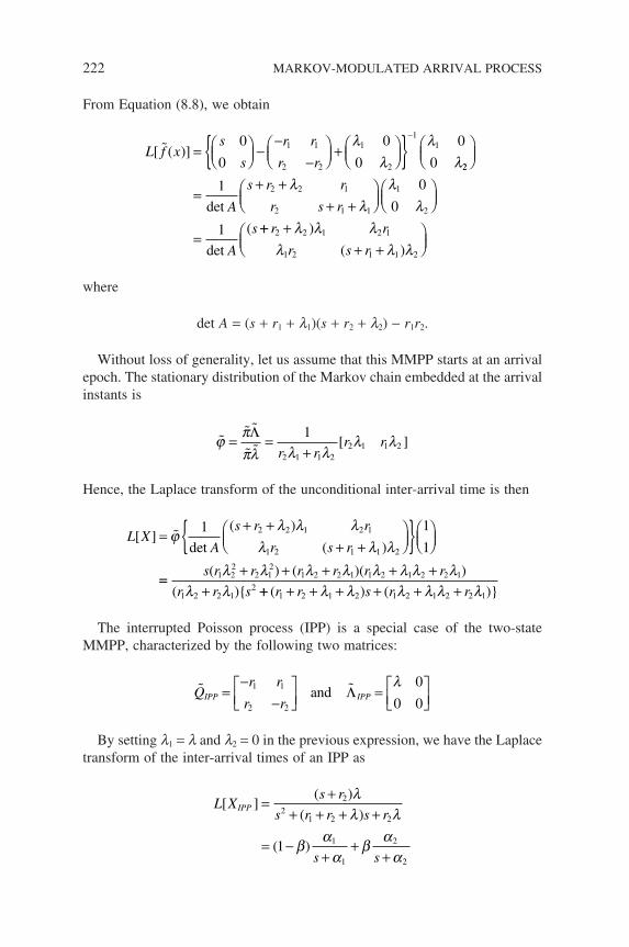
222 MARKOV-MODULATED ARRIVAL PROCESS
From Equation (8.8), we obtain
L f xs
s
r r
r r[ ( )] =
−
−−
+
−0
0
0
0
0
01 1
2 2
1
2
11λ
λλ
λ22
2 2 1
2 1 1
1
2
1 0
0
1
=+ +
+ +
=
det
det
(
A
s r r
r s r
A
s
λλ
λλ
++ ++ +
r r
r s r2 2 1 2 1
1 2 1 1 2
λ λ λλ λ λ
)
( )
where
det A = (s + r1 + l1)(s + r2 + l2) − r1r2.
Without loss of generality, let us assume that this MMPP starts at an arrival epoch. The stationary distribution of the Markov chain embedded at the arrival instants is
ϕ π
πλ λ λλ λ= =
+Λ 1
2 1 1 22 1 1 2
r rr r[ ]
Hence, the Laplace transform of the unconditional inter-arrival time is then
L XA
s r r
r s r[ ]
det
( )
( )=
+ ++ +
ϕλ λ λ
λ λ λ1 1
12 2 1 2 1
1 2 1 1 2
==+ + + + +
+s r r r r r r
r r s
( ) ( )( )
( )1 2
22 1
21 2 2 1 1 2 1 2 2 1
1 2 2 12
λ λ λ λ λ λ λ λλ λ ++ + + + + + +( ) ( )r r s r r1 2 1 2 1 2 1 2 2 1λ λ λ λ λ λ
The interrupted Poisson process (IPP) is a special case of the two-state MMPP, characterized by the following two matrices:
Qr r
r rIPP IPP=
−−
=
1 1
2 2
0
0 0and Λ
λ
By setting l1 = l and l2 = 0 in the previous expression, we have the Laplace transform of the inter-arrival times of an IPP as
L Xs r
s r r s r
s s
IPP[ ]( )
( )
( )
=+
+ + + +
= −+
++
2
21 2 2
1
1
2
2
1
λλ λ
β αα
β αα
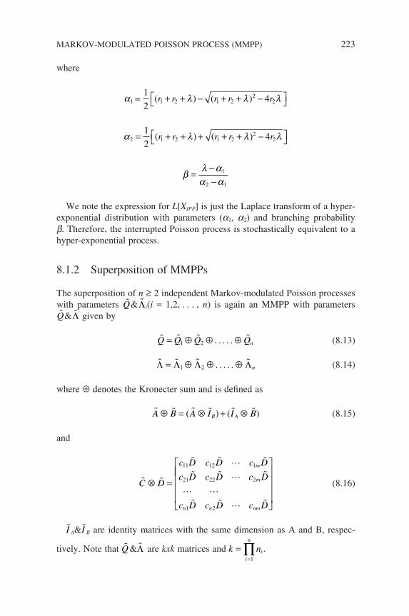
where
α λ λ λ1 1 2 1 22
21
24= + + − + + − ( ) ( )r r r r r
α λ λ λ2 1 2 1 22
21
24= + + + + + − ( ) ( )r r r r r
β λ αα α
=−−
1
2 1
We note the expression for L[XIPP] is just the Laplace transform of a hyper-exponential distribution with parameters (a1, a2) and branching probability b. Therefore, the interrupted Poisson process is stochastically equivalent to a hyper-exponential process.
8.1.2 Superposition of MMPPs
The superposition of n ≥ 2 independent Markov-modulated Poisson processes with parameters Q& Λi(i = 1,2, . . . , n) is again an MMPP with parameters Q& Λ given by
Q Q Q Qn= ⊕ ⊕ ⊕1 2 . . . . . (8.13)
Λ Λ Λ Λ= ⊕ ⊕ ⊕1 2 . . . . . n (8.14)
where ⊕ denotes the Kronecter sum and is defi ned as
A B A I I BB A⊕ = ⊗ + ⊗( ) ( ) (8.15)
and
C D
c D c D c D
c D c D c D
c D c D c D
m
m
n n nm
⊗ =
11 12 1
21 22 2
1 2
(8.16)
I A& I B are identity matrices with the same dimension as A and B, respec-
tively. Note that Q & Λ are kxk matrices and k nii
n
==
∏1
.
MARKOV-MODULATED POISSON PROCESS (MMPP) 223
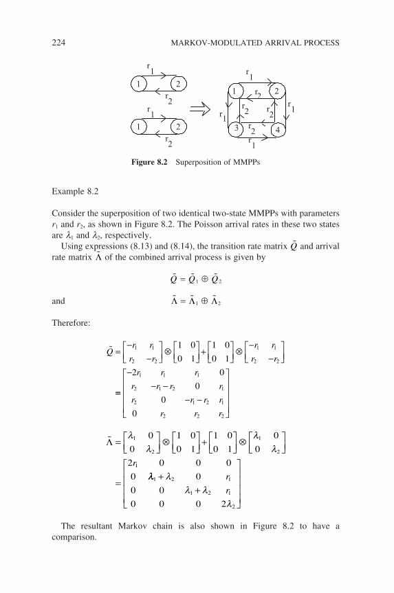
224 MARKOV-MODULATED ARRIVAL PROCESS
Example 8.2
Consider the superposition of two identical two-state MMPPs with parameters r1 and r2, as shown in Figure 8.2. The Poisson arrival rates in these two states are l1 and l2, respectively.
Using expressions (8.13) and (8.14), the transition rate matrix Q and arrival rate matrix Λ of the combined arrival process is given by
Q = Q1 ⊕ Q2
and Λ = Λ1 ⊕ Λ2
Therefore:
Qr r
r r
r r
r r=
−−
⊗
+
⊗−
−
1 1
2 2
1 1
2 2
1 0
0 1
1 0
0 1
==
−− −
− −
2 0
0
0
0
1 1 1
2 1 2 1
2 1 2 1
2 2 2
r r r
r r r r
r r r r
r r r
Λ =
⊗
+
⊗
=
λλ
λλ
1
2
1
2
1
0
0
1 0
0 1
1 0
0 1
0
0
2 0 0 0
0
r
λλ λλ λ
λ
1 2 1
1 2 1
2
0
0 0
0 0 0 2
++
r
r
The resultant Markov chain is also shown in Figure 8.2 to have a comparison.
r1
r1
1 2
3 4
r2
r1
r1r
2 r2
r2
r1
1 2r2
1 2r2
r1
Figure 8.2 Superposition of MMPPs
8.1.3 MMPP/G/1
This is a queueing system where customers arrive according to an MMPP and are served by a single server with a general service time distribution x(t). The waiting queue is infi nite and customers are served according to their order of arrival, as shown in Figure 8.3.
The MMPP is characterized by the matrices Q& Λ, and the service time distribution has a mean 1/m and Laplace transform X(s). The utilization of the system is
ρ πλ µ π λ π λ π λµ
= =+ + + 1 1 2 2 . . . m m
Consider the successive epochs of departure tk : k ≥ 0. Firstly, let us defi ne Nk&Jk to be the number of customers in the system and the state of the MMPP at tk respectively, then the sequence (Nk, Jk, tk+1 − tk) : k ≥ 0 forms a semi-Markov sequence with the transition probability matrix:
Q
B B B
A A A
A A=
0 1 2
0 1 2
0 10 (8.17)
where
A P n t d x t B Q An n n( ) ( , ) ( ( )) ( ) ( )ςς
= = − ∞∫ −
0
1and Λ Λ (8.18)
If we defi ne wi(t) to be the joint probability that the MMPP is in phase i and that a customer who arrives at that time would wait less than or equal to t before receiving service, then the virtual delay distribution matrix, W(t) = (wi(t)) is given by the following expression in Laplace transform:
1
i
m
Markov Chainλ
λ
λ1 m
i
Figure 8.3 MMPP/G/1
MARKOV-MODULATED POISSON PROCESS (MMPP) 225
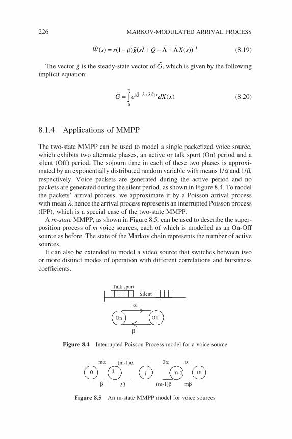
226 MARKOV-MODULATED ARRIVAL PROCESS
W s s g sI Q X s( ) ( ) ( ( ))= − + − + −1 1ρ Λ Λ (8.19)
The vector g is the steady-state vector of G, which is given by the following implicit equation:
G e dX xQ G x= − +
∞
∫ ( ) ( )Λ Λ
0
(8.20)
8.1.4 Applications of MMPP
The two-state MMPP can be used to model a single packetized voice source, which exhibits two alternate phases, an active or talk spurt (On) period and a silent (Off) period. The sojourn time in each of these two phases is approxi-mated by an exponentially distributed random variable with means 1/a and 1/b, respectively. Voice packets are generated during the active period and no packets are generated during the silent period, as shown in Figure 8.4. To model the packets’ arrival process, we approximate it by a Poisson arrival process with mean l, hence the arrival process represents an interrupted Poisson process (IPP), which is a special case of the two-state MMPP.
A m-state MMPP, as shown in Figure 8.5, can be used to describe the super-position process of m voice sources, each of which is modelled as an On-Off source as before. The state of the Markov chain represents the number of active sources.
It can also be extended to model a video source that switches between two or more distinct modes of operation with different correlations and burstiness coeffi cients.
On Off
α
β
Talk spurtSilent
Figure 8.4 Interrupted Poisson Process model for a voice source
0 1 i m-1 m
β
αmα (m-1)α 2α
2β (m-1)β mβ
Figure 8.5 An m-state MMPP model for voice sources
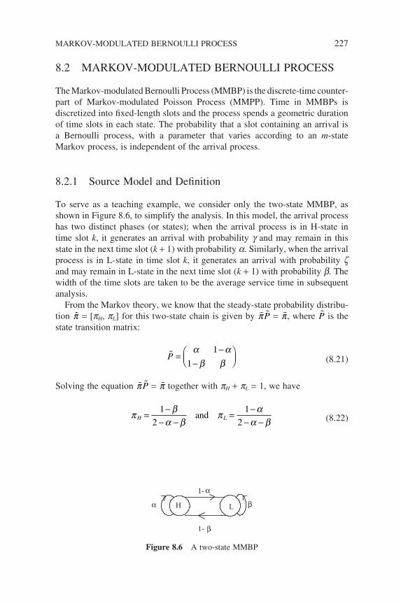
8.2 MARKOV-MODULATED BERNOULLI PROCESS
The Markov-modulated Bernoulli Process (MMBP) is the discrete-time counter-part of Markov-modulated Poisson Process (MMPP). Time in MMBPs is discretized into fi xed-length slots and the process spends a geometric duration of time slots in each state. The probability that a slot containing an arrival is a Bernoulli process, with a parameter that varies according to an m-state Markov process, is independent of the arrival process.
8.2.1 Source Model and Defi nition
To serve as a teaching example, we consider only the two-state MMBP, as shown in Figure 8.6, to simplify the analysis. In this model, the arrival process has two distinct phases (or states); when the arrival process is in H-state in time slot k, it generates an arrival with probability g and may remain in this state in the next time slot (k + 1) with probability a. Similarly, when the arrival process is in L-state in time slot k, it generates an arrival with probability z and may remain in L-state in the next time slot (k + 1) with probability b. The width of the time slots are taken to be the average service time in subsequent analysis.
From the Markov theory, we know that the steady-state probability distribu-tion π = [pH, pL] for this two-state chain is given by π P = π, where P is the state transition matrix:
P =−
−
α αβ β
1
1 (8.21)
Solving the equation π P = π together with pH + pL = 1, we have
π βα β
π αα βH L=
−− −
=−
− −1
2
1
2and (8.22)
H L
1-
1-
α β
α
β
Figure 8.6 A two-state MMBP
MARKOV-MODULATED BERNOULLI PROCESS 227
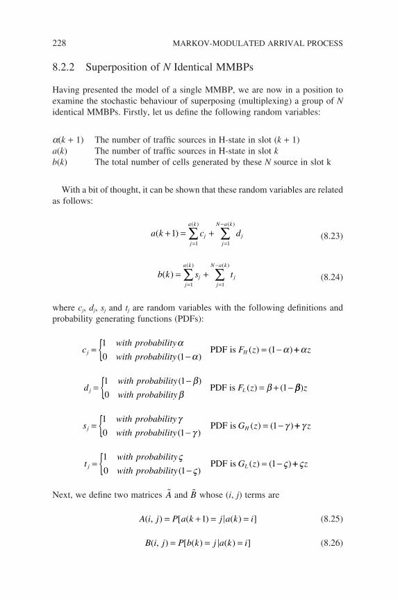
228 MARKOV-MODULATED ARRIVAL PROCESS
8.2.2 Superposition of N Identical MMBPs
Having presented the model of a single MMBP, we are now in a position to examine the stochastic behaviour of superposing (multiplexing) a group of N identical MMBPs. Firstly, let us defi ne the following random variables:
a(k + 1) The number of traffi c sources in H-state in slot (k + 1)a(k) The number of traffi c sources in H-state in slot kb(k) The total number of cells generated by these N source in slot k
With a bit of thought, it can be shown that these random variables are related as follows:
a k c djj
a k
jj
N a k
( )( ) ( )
+ = += =
−
∑ ∑11 1
(8.23)
b k s tjj
a k
jj
N a k
( )( ) ( )
= += =
−
∑ ∑1 1
(8.24)
where cj, dj, sj and tj are random variables with the following defi nitions and probability generating functions (PDFs):
cwith probability
with probabilityF zj H=
− = −1
0 11
αα
α( )
( ) ( )PDF is ++ αz
dwith probability
with probabilityF zj L=
− = + −1 1
01
( )( ) (
ββ
βPDF is ββ)z
swith probability
with probabilityG zj H=
− = −1
0 11
γγ
γ( )
( ) ( )PDF is ++ γ z
twith probability
with probabilityG zj L=
− = −1
0 11
ςς
ς( )
( ) ( )PDF is ++ ςz
Next, we defi ne two matrices A and B whose (i, j) terms are
A i j P a k j a k i( , ) [ ( ) ( ) ]= + = =1 (8.25)
B i j P b k j a k i( , ) [ ( ) ( ) ]= = = (8.26)
Matrix A gives the correlation between the number of H-state MMBP sources in adjacent time slots, and matrix B shows the relationship between the number of arrivals and the number of H-state MMBP sources in a particular time slot. Both matrices are required in subsequent analysis.
To facilitate the build-up of these two matrices, we see that the z-transform of the ith row of these two matrices are given respectively as
A z P a k j a k i z
F z F z
in
j
Hi
LN i
( ) [ ( ) ( ) ]
( ) ( )
= + = =
= ⋅=
∞
−
∑ 10
(8.27)
B z P b k j a k i z
G z G z
in
j
Hi
LN i
( ) [ ( ) ( ) ]
( ) ( )
= = =
= ⋅=
∞
−
∑0
(8.28)
where f i means the multiplication of i times.The steady-state number of arrivals per time slot is then given by
λ π πtot H H z L L zN G z G z= ′ + ′= =[ ( ) ( ) ]1 1 (8.29)
8.2.3 ΣMMBP/D/1
In this section, we take a look at a queueing system where an infi nite waiting queue is fed by a group of N identical MMBP sources and served by a deter-ministic server. Without loss of generality, we assume that the width of a time slot is equal to the constant service time (1/m) and is equal to 1 unit of measure.
Having obtained the correlation expressions (8.27) and (8.28) for those random variables presented in the last section, we are now in a position to examine the evolution of queue length in slot (k + 1), that is q(k + 1). Firstly, let us defi ne the z-transform of the joint probability P[q(k + 1) = j, a(k + 1) = i]:
Q z P q k j a k i z
z
ik j
j
jik j
j
+
=
∞
+
=
∞
= + = + =
=
∑
∑
1
0
1
0
1 1( ) [ ( ) , ( ) ]
π (8.30)
MARKOV-MODULATED BERNOULLI PROCESS 229
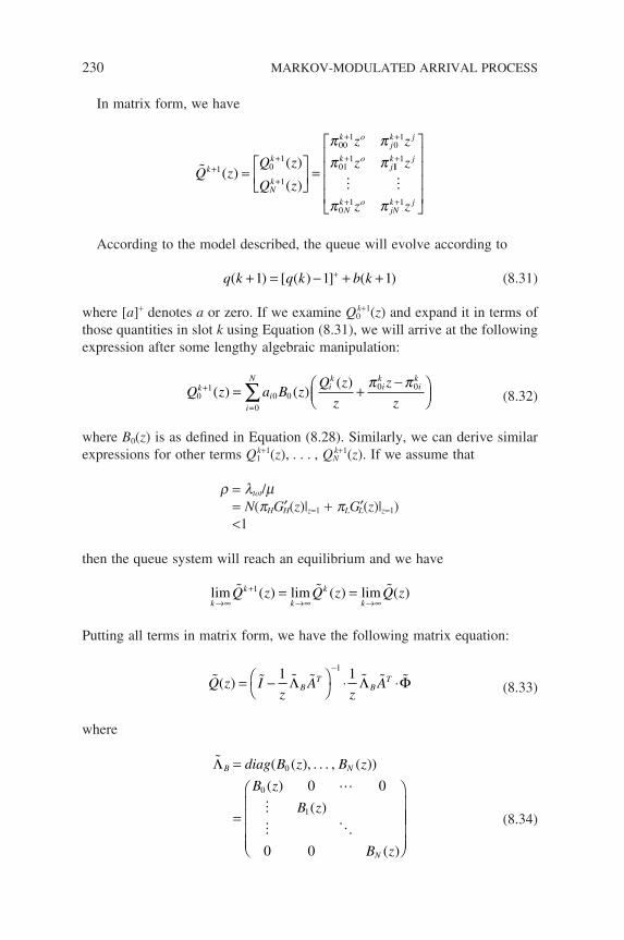
230 MARKOV-MODULATED ARRIVAL PROCESS
In matrix form, we have
Q zQ z
Q z
z z
zk
k
Nk
k ojk j
k oj+
+
+
+ +
+
=
=1 01
1
001
01
011
( )( )
( )
π ππ π 11
1
01 1
k j
Nk o
jNk j
z
z z
+
+ +
π π
According to the model described, the queue will evolve according to
q k q k b k( ) [ ( ) ] ( )+ = − + ++1 1 1 (8.31)
where [a]+ denotes a or zero. If we examine Q0k+1(z) and expand it in terms of
those quantities in slot k using Equation (8.31), we will arrive at the following expression after some lengthy algebraic manipulation:
Q z a B zQ z
z
z
zk
ii
Nik
ik
ik
01
0 00
0 0+
=
= +−
∑( ) ( )
( ) π π (8.32)
where B0(z) is as defi ned in Equation (8.28). Similarly, we can derive similar expressions for other terms Q1
k+1(z), . . . , QNk+1(z). If we assume that
r = ltot/m = N(pHG′H(z)|z=1 + pLG′L(z)|z=1) <1
then the queue system will reach an equilibrium and we have
lim ( ) lim ( ) lim ( )k
k
k
k
kQ z Q z Q z
→∞
+
→∞ →∞= = 1
Putting all terms in matrix form, we have the following matrix equation:
Q z I
zA
zAB
TB
T( ) = −
⋅ ⋅
−1 11
Λ Λ Φ (8.33)
where
ΛB N
N
diag B z B z
B z
B z
B z
=
=
( ( ), . . . , ( ))
( )
( )
( )
0
0
1
0 0
0 0
(8.34)
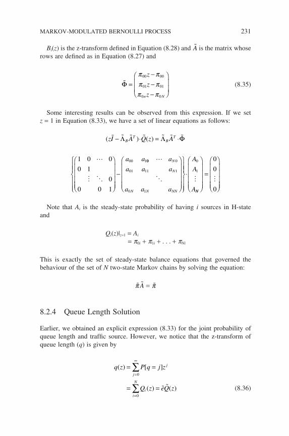
Bi(z) is the z-transform defi ned in Equation (8.28) and A is the matrix whose rows are defi ned as in Equation (8.27) and
Φ =−−−
π ππ ππ π
00 00
01 01
0 0
z
z
zn N
(8.35)
Some interesting results can be observed from this expression. If we set z = 1 in Equation (8.33), we have a set of linear equations as follows:
( ) ( )zI A Q z A
a a
BT
BT
− ⋅ = ⋅
−
Λ Λ Φ
1 0 0
0 1
0
0 0 1
00 100 0
01 11 1
0 1
0
1
a
a a a
a a a
A
A
A
N
N
N N NN
⋅
NN
=
0
0
0
Note that Ai is the steady-state probability of having i sources in H-state and
Qi(z)|z=1 = Ai
= p0i + p1i + . . . + pNi
This is exactly the set of steady-state balance equations that governed the behaviour of the set of N two-state Markov chains by solving the equation:
π A = π
8.2.4 Queue Length Solution
Earlier, we obtained an explicit expression (8.33) for the joint probability of queue length and traffi c source. However, we notice that the z-transform of queue length (q) is given by
q z P q j z
Q z eQ z
j
j
ii
N
( ) [ ]
( ) ( )
= =
= =
=
∞
=
∑
∑0
0
(8.36)
MARKOV-MODULATED BERNOULLI PROCESS 231
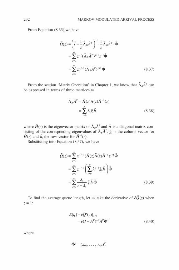
232 MARKOV-MODULATED ARRIVAL PROCESS
From Equation (8.33) we have
Q z Iz
Az
A
z A z
BT
BT
jB
T j
j
( )
( )
= −
⋅ ⋅
=
−
− + −
=
1 11
1 1
0
Λ Λ Φ
Λ Φ∞∞
− − +
=
∞
∑
∑= z AjB
T j
j
1 1
0
( ) Λ Φ (8.37)
From the section ‘Matrix Operation’ in Chapter 1, we know that ΛBAT can
be expressed in terms of three matrices as
Λ ΛBT
i i ii
N
A H z z H z
g h
=
=
−
=∑
( ) ( ) ( )1
0
λ (8.38)
where H(z) is the eigenvector matrix of ΛBAT and Λ is a diagonal matrix con-
sisting of the corresponding eigenvalues of ΛBAT. gi is the column vector for
H(z) and hi the row vector for H−1(z).Substituting into Equation (8.37), we have
Q z z H z z H
z g h
j j
j
jij
h ii
N
( ) ( ( ) ( ) )=
=
− − − +
=
∞
− − +
=
∑ 1 1 1
0
1 1
0
Λ Φ
λ∑∑∑
∑
=−
=
∞
=
∞
Φ
Φ
j
i
ii i
j zg h
0
0
λλ
(8.39)
To fi nd the average queue length, let us take the derivative of e Q(z) when z = 1:
E q eQ z
e I A A
z
T T
[ ] ( )
( )
= ′
= − ′=
−
1
1 Φ (8.40)
where
Φ′ = (p00, . . . , p0N)T.
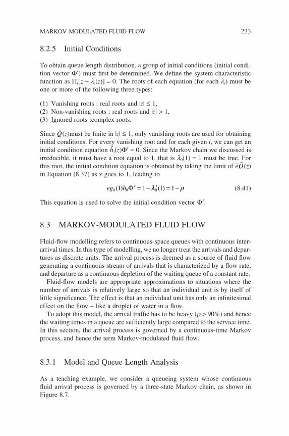
8.2.5 Initial Conditions
To obtain queue length distribution, a group of initial conditions (initial condi-tion vector Φ′) must fi rst be determined. We defi ne the system characteristic function as Πi[z − li(z)] = 0. The roots of each equation (for each li) must be one or more of the following three types:
(1) Vanishing roots : real roots and |z| ≤ 1,(2) Non-vanishing roots : real roots and |z| > 1,(3) Ignored roots :complex roots.
Since Q(z)must be fi nite in |z| ≤ 1, only vanishing roots are used for obtaining initial conditions. For every vanishing root and for each given i, we can get an initial condition equation hi(z)Φ′ = 0. Since the Markov chain we discussed is irreducible, it must have a root equal to 1, that is l0(1) = 1 must be true. For this root, the initial condition equation is obtained by taking the limit of e Q(z) in Equation (8.37) as z goes to 1, leading to
eg h0 0 01 1 1 1( ) ( )′ = − ′ = −Φ λ ρ (8.41)
This equation is used to solve the initial condition vector Φ′.
8.3 MARKOV-MODULATED FLUID FLOW
Fluid-fl ow modelling refers to continuous-space queues with continuous inter-arrival times. In this type of modelling, we no longer treat the arrivals and depar-tures as discrete units. The arrival process is deemed as a source of fl uid fl ow generating a continuous stream of arrivals that is characterized by a fl ow rate, and departure as a continuous depletion of the waiting queue of a constant rate.
Fluid-fl ow models are appropriate approximations to situations where the number of arrivals is relatively large so that an individual unit is by itself of little signifi cance. The effect is that an individual unit has only an infi nitesimal effect on the fl ow – like a droplet of water in a fl ow.
To adopt this model, the arrival traffi c has to be heavy (r > 90%) and hence the waiting times in a queue are suffi ciently large compared to the service time. In this section, the arrival process is governed by a continuous-time Markov process, and hence the term Markov-modulated fl uid fl ow.
8.3.1 Model and Queue Length Analysis
As a teaching example, we consider a queueing system whose continuous fl uid arrival process is governed by a three-state Markov chain, as shown in Figure 8.7.
MARKOV-MODULATED FLUID FLOW 233
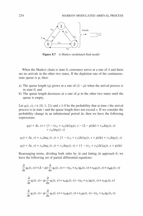
234 MARKOV-MODULATED ARRIVAL PROCESS
When the Markov chain is state 0, customers arrive at a rate of l and there are no arrivals in the other two states. If the depletion rate of the continuous-state queue is m, then:
a) The queue length (q) grows at a rate of (l − m) when the arrival process is in state 0, and
b) The queue length decreases at a rate of m in the other two states until the queue is empty.
Let qi(t, x), i ∈ 0, 1, 2) and x ≥ 0 be the probability that at time t the arrival process is in state i and the queue length does not exceed x. If we consider the probability change in an infi nitesimal period ∆t, then we have the following expressions:
q0(t + ∆t, x) = 1 − (r01 + r02)∆tq0(t, x − (l − m)∆t) + r10∆tq1(t, x) + r20∆tq2(t, x)
q1(t + ∆t, x) = r01∆tq0 (t, x) + 1 − (r10 + r12)∆tq1(t, x + m)∆t) + r21∆tq2(t, x)
q2(t + ∆t, x) = r02∆tq0 (t, x) + r12∆tq1(t, x) + 1 − (r21 + r20)∆tq2(t, x + m)∆t)
Rearranging terms, dividing both sides by ∆t and letting ∆t approach 0, we have the following set of partial differential equations:
∂∂
+ −∂∂
= − + + +t
q t xx
q t x r r q t x r q t x r0 0 01 02 0 10 1 2( , ) ( ) ( , ) ( ) ( , ) ( , )λ µ 00 2q t x( , )
∂∂
−∂∂
= − + +t
q t xx
q t x r q t x r r q t x r q t1 1 01 0 10 12 1 21 2( , ) ( , ) ( , ) ( ) ( , ) (µ ,, )x
∂∂
−∂∂
= + − +t
q t xx
q t x r q t x r q t x r r q t2 2 02 0 12 1 21 20 2( , ) ( , ) ( , ) ( , ) ( ) (µ ,, )x
1
0 2
r01
r12
r20
r10
r21
r12
λ
Arrivals
Figure 8.7 A Markov-modulated fl uid model
Since we are interested in the steady-state behaviour of a queueing system, we set
∂∂
=t
q t xi ( , ) 0
hence we can drop the time parameter t and we have
( ) ( , ) ( ) ( , ) ( , ) ( , )λ µ− = − + + +d
dxq t x r r q t x r q t x r q t x0 01 02 0 10 1 20 2 (8.42)
−∂∂
= − + +µx
q t x r q t x r r q t x r q t x1 01 0 10 12 1 21 2( , ) ( , ) ( ) ( , ) ( , ) (8.43)
−∂∂
= + − +µx
q t x r q t x r q t x r r q t x2 02 0 12 1 21 20 2( , ) ( , ) ( , ) ( ) ( , ) (8.44)
The qi(x) is the steady-state probability that the arrival process is in state i and the queue length does not exceed x. In matrix form, we have
Dd
dxQ x MQ x( ) ( )= (8.45)
where
Q x q x q x q x T( ) ( ( ), ( ), ( ))= 0 1 2
D diag= − − −[( ), , ]λ µ µ µ
Mr r r r
r r r r
r r r r
=− +
− +− +
( )
( )
( )
01 02 10 20
01 10 12 21
02 12 21 20
From the section ‘Matrix Calculus’ in Chapter 1, we see that the general solution of Equation (8.45) is
Q x Q a g ei iz xi( ) ( )= ∞ + ∑ (8.46)
where the z′is are eigenvalues of D−1 M in the left-half complex plane (i.e. Re(zi) > 0) and gi are eigenvectors satisfying
zigi = D−1 M
MARKOV-MODULATED FLUID FLOW 235
236 MARKOV-MODULATED ARRIVAL PROCESS
The coeffi cient ai can be determined by boundary conditions. We see from the proceeding analysis that the fl uid fl ow model has transformed the queueing problem into a set of differential equations instead of the usual linear equations.
8.3.2 Applications of Fluid Flow Model to ATM
The Markov-modulated fl uid fl ow model is a suitable model for analysing traffi c presented to a switch in an ATM network. In ATM, packets are fi xed-sized cells of 53 bytes in length and the transmission speeds are probably of the order of a few gigabits per second, hence the transmission time of an indi-vidual cell is like a drop of water in the fl uid fl ow model and so its effect is infi nitesimal.
Another important advantage of the fl uid-fl ow model is its ease of simula-tion. As discussed earlier, the transmission time of a cell is on a very fi ne scale, hence the simulation of cell-arrival events would consume vast CPU and pos-sible memory resources, even for a simulation of a few minutes. A statistically meaningful simulation may not be feasible. In contrast, a fl uid-fl ow model simulation deals with the rate of arrivals and rate of transmission and can be simulated over much longer time periods.
8.4 NETWORK CALCULUS
In this section, we are presenting an introductory overview of a new paradigm of queueing analysis called Network Calculus, which analyses queues from a very different perspective from that of classical queueing theory. For more detail, students should refer to the references.
Network Calculus is a new methodology that works with deterministic bounds on the performance measures of a queue. It was pioneered by Rene L. Cruz (Cruz 1991) for analysing delay and buffering requirements of network elements, and further developed by Jean-Yves Boudec (Boudec and Thiran 2002) and Cheng-Shang Chang (Chang 2000). It is a form of deterministic queueing theory for the reasons explained below.
In classical queueing theory, the traffi c that enters a queueing system (or queueing network) is always characterized by a stochastic process; notably Poisson or other independent arrival processes. The associated calculus is then applied to derive the performance measures. The calculus here refers to the stochastic and mathematical theories that are associated with the arrival and service processes. The queueing results are often complex or the exact analysis intractable for realistic models. In addition, the traffi c arrival processes are often correlated and hence render the Poisson or other simple arrival model unrealistic.
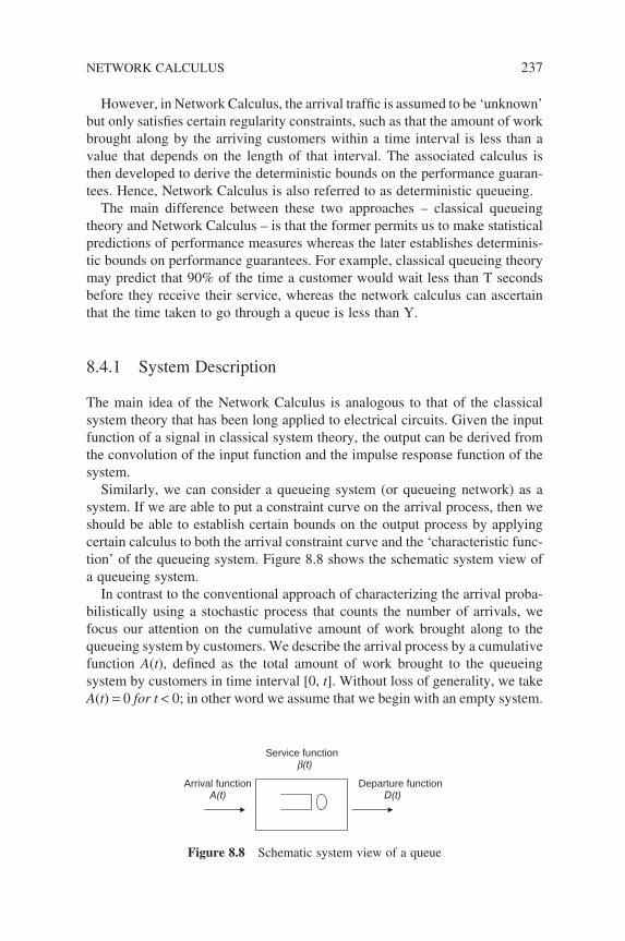
However, in Network Calculus, the arrival traffi c is assumed to be ‘unknown’ but only satisfi es certain regularity constraints, such as that the amount of work brought along by the arriving customers within a time interval is less than a value that depends on the length of that interval. The associated calculus is then developed to derive the deterministic bounds on the performance guaran-tees. Hence, Network Calculus is also referred to as deterministic queueing.
The main difference between these two approaches – classical queueing theory and Network Calculus – is that the former permits us to make statistical predictions of performance measures whereas the later establishes determinis-tic bounds on performance guarantees. For example, classical queueing theory may predict that 90% of the time a customer would wait less than T seconds before they receive their service, whereas the network calculus can ascertain that the time taken to go through a queue is less than Y.
8.4.1 System Description
The main idea of the Network Calculus is analogous to that of the classical system theory that has been long applied to electrical circuits. Given the input function of a signal in classical system theory, the output can be derived from the convolution of the input function and the impulse response function of the system.
Similarly, we can consider a queueing system (or queueing network) as a system. If we are able to put a constraint curve on the arrival process, then we should be able to establish certain bounds on the output process by applying certain calculus to both the arrival constraint curve and the ‘characteristic func-tion’ of the queueing system. Figure 8.8 shows the schematic system view of a queueing system.
In contrast to the conventional approach of characterizing the arrival proba-bilistically using a stochastic process that counts the number of arrivals, we focus our attention on the cumulative amount of work brought along to the queueing system by customers. We describe the arrival process by a cumulative function A(t), defi ned as the total amount of work brought to the queueing system by customers in time interval [0, t]. Without loss of generality, we take A(t) = 0 for t < 0; in other word we assume that we begin with an empty system.
Arrival function A(t)
Departure function D(t)
Service function b(t)
Figure 8.8 Schematic system view of a queue
NETWORK CALCULUS 237
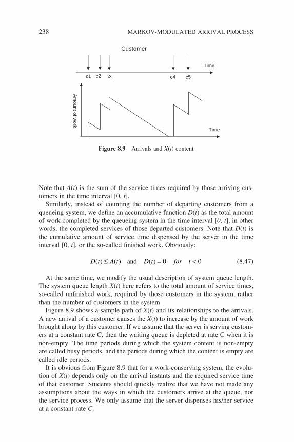
238 MARKOV-MODULATED ARRIVAL PROCESS
Note that A(t) is the sum of the service times required by those arriving cus-tomers in the time interval [0, t].
Similarly, instead of counting the number of departing customers from a queueing system, we defi ne an accumulative function D(t) as the total amount of work completed by the queueing system in the time interval [0, t], in other words, the completed services of those departed customers. Note that D(t) is the cumulative amount of service time dispensed by the server in the time interval [0, t], or the so-called fi nished work. Obviously:
D t A t D t for t( ) ( ) ( )≤ = <and 0 0 (8.47)
At the same time, we modify the usual description of system queue length. The system queue length X(t) here refers to the total amount of service times, so-called unfi nished work, required by those customers in the system, rather than the number of customers in the system.
Figure 8.9 shows a sample path of X(t) and its relationships to the arrivals. A new arrival of a customer causes the X(t) to increase by the amount of work brought along by this customer. If we assume that the server is serving custom-ers at a constant rate C, then the waiting queue is depleted at rate C when it is non-empty. The time periods during which the system content is non-empty are called busy periods, and the periods during which the content is empty are called idle periods.
It is obvious from Figure 8.9 that for a work-conserving system, the evolu-tion of X(t) depends only on the arrival instants and the required service time of that customer. Students should quickly realize that we have not made any assumptions about the ways in which the customers arrive at the queue, nor the service process. We only assume that the server dispenses his/her service at a constant rate C.
Customer
c1 c2 c3 c4 c5
Time
Time
Am
ount of work
Figure 8.9 Arrivals and X(t) content
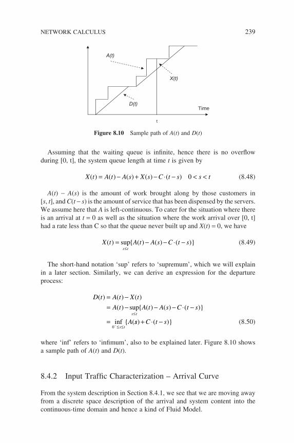
Assuming that the waiting queue is infi nite, hence there is no overfl ow during [0, t], the system queue length at time t is given by
X t A t A s X s C t s s t( ) ( ) ( ) ( ) ( )= − + − ⋅ − < <0 (8.48)
A(t) − A(s) is the amount of work brought along by those customers in [s, t], and C(t − s) is the amount of service that has been dispensed by the servers. We assume here that A is left-continuous. To cater for the situation where there is an arrival at t = 0 as well as the situation where the work arrival over [0, t] had a rate less than C so that the queue never built up and X(t) = 0, we have
X t A t A s C t ss t
( ) sup ( ) ( ) ( )= − − ⋅ −≤
(8.49)
The short-hand notation ‘sup’ refers to ‘supremum’, which we will explain in a later section. Similarly, we can derive an expression for the departure process:
D t A t X t
A t A t A s C t s
As t
s t
( ) ( ) ( )
( ) sup ( ) ( ) ( )
inf (
= −= − − − ⋅ −
=≤
≤ ≤−0ss C t s) ( )+ ⋅ − (8.50)
where ‘inf’ refers to ‘infi mum’, also to be explained later. Figure 8.10 shows a sample path of A(t) and D(t).
8.4.2 Input Traffi c Characterization – Arrival Curve
From the system description in Section 8.4.1, we see that we are moving away from a discrete space description of the arrival and system content into the continuous-time domain and hence a kind of Fluid Model.
Time
A(t)
t
D(t)
X(t)
Figure 8.10 Sample path of A(t) and D(t)
NETWORK CALCULUS 239
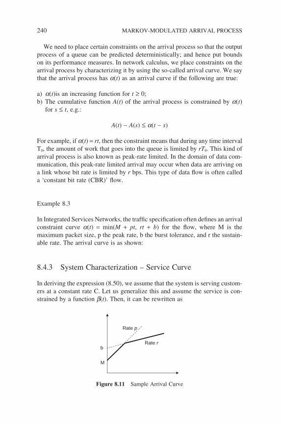
240 MARKOV-MODULATED ARRIVAL PROCESS
We need to place certain constraints on the arrival process so that the output process of a queue can be predicted deterministically; and hence put bounds on its performance measures. In network calculus, we place constraints on the arrival process by characterizing it by using the so-called arrival curve. We say that the arrival process has a(t) as an arrival curve if the following are true:
a) a(t)is an increasing function for t ≥ 0;b) The cumulative function A(t) of the arrival process is constrained by a(t)
for s ≤ t, e.g.:
A(t) − A(s) ≤ a(t − s)
For example, if a(t) = rt, then the constraint means that during any time interval T0, the amount of work that goes into the queue is limited by rT0. This kind of arrival process is also known as peak-rate limited. In the domain of data com-munication, this peak-rate limited arrival may occur when data are arriving on a link whose bit rate is limited by r bps. This type of data fl ow is often called a ‘constant bit rate (CBR)’ fl ow.
Example 8.3
In Integrated Services Networks, the traffi c specifi cation often defi nes an arrival constraint curve a(t) = min(M + pt, rt + b) for the fl ow, where M is the maximum packet size, p the peak rate, b the burst tolerance, and r the sustain-able rate. The arrival curve is as shown:
8.4.3 System Characterization – Service Curve
In deriving the expression (8.50), we assume that the system is serving custom-ers at a constant rate C. Let us generalize this and assume the service is con-strained by a function b(t). Then, it can be rewritten as
M
b
Rate p
Rate r
Figure 8.11 Sample Arrival Curve
D t A s t s
A ts t
( ) inf ( ) ( )
( )( )
= + −
= ⊗− ≤ ≤0
β
β (8.51)
The ⊗ notation is the so-called convolution operation in min-plus algebra. The expression resembles the convolution of the input signal function and the impulse function to yield the output process in system theory, except the min-plus convolution operation here replaces multiplication with addition, and addition with the computation of infi mum.
This leads us to the defi nition of the service curve. We say that a system offers to the input process a service curve b if and only if
D t A t( ) ( )( )= ⊗ β (8.52)
From Equation (8.51), we see that given the characterization of arrival process in terms of arrival curve and the characterization of service process in terms of service curve, the departing process of a queue can be calculated deterministically. This is the essence of network calculus.
8.4.4 Min-Plus Algebra
In previous sections, we introduced the notions of infi mum and supremum. We shall clarify these terms here. Students can refer to (Boudec and Thiran 2002) for more detail.
Conceptually, infi mum and supremum are similar to the minimum and maximum of a set respectively with some minor differences. Consider a non-empty set S s ∈ S; it is said to be bounded from below if there is a number N1 such that s ≥ N1. That number N1 is the infi mum of S. If N1 happens to be an element in set S and is smaller than any other elements in the set, then is called the minimum of S. For example, the closed and open interval of [a, b] and (a, b) have the same infi mum, but (a, b) does not have a minimum.
Similarly, S is said to be bounded from above if there is a number N2 such that S ≤ N2, then N2 is the supremum of S. If it happens to be an element in the set and is larger than any other elements in the set, it is called the maximum of S. For example, sup [4,5,6] = max [4,5,6] = 6.
In conventional linear system theory, the convolution between two functions is defi ned as
(f ⊗ g)(t) = −∞
∞
∫ f(t − s)g(s)ds
However, in min-plus algebra, the usual addition operator is replaced by the inf (or min) operator and the multiplication operator by the addition operator. Hence, the convolution of two functions is given as
NETWORK CALCULUS 241
242 MARKOV-MODULATED ARRIVAL PROCESS
( )( ) inf [ ( ) ( )]f g t f s g t ss t
⊗ = + −≤ ≤0
(8.53)
Similar to the conventional convolution, the min-plus convolution is associa-tive, commutative and distributive as
(f ⊗ g) ⊗ h = f ⊗ (g ⊗ h) Associativity
f ⊗ g = g = g ⊗ f Commutativity
[inf(f, g)] ⊗ h = inf(f ⊗ h, g ⊗ h) Distributivity
9Flow and Congestion Control
Today, we often experience congestion in modern cities, in terms of long queues of cars, buses and people waiting for services. Congestion is usually caused by unpredictable events. Although the daily rush hour is semi-predict-able, congestion can also be random due to breakdowns and accidents that cause delays and long queues stretching for long distances. Therefore, a control mechanism might be implemented, such as using traffi c lights to delay access to a junction or by restricting access to crowded areas in central business dis-tricts through tolls and congestion charges.
In general, the communication network is similar to our everyday experi-ences and consists of fi nite resources, such as bandwidth, buffer capacity for packets and transmission capacity that depend on traffi c control mechanisms to alleviate congestion problems.
There are specifi c requirement guarantees, referred to as Quality of Service (QoS), specifi ed for each traffi c fl ow. When the offered traffi c load from the user to the network exceeds the design limit and the required network resources, congestion will often occur. In this section, we introduce several specifi c examples, where queueing theory has been successfully applied to study the behaviour of the network under these extreme conditions. We describe key parameters of performances, i.e. throughput g and time delay E[T]. It is impor-tant to examine the basic functioning of the network, as shown in Figure 9.1.
9.1 INTRODUCTION
The topic of congestion control has a long history (Schwartz 1987). A simple mechanism for preventing congestion is fl ow control, which involves
Queueing Modelling Fundamentals Second Edition Ng Chee-Hock and Soong Boon-Hee© 2008 John Wiley & Sons, Ltd
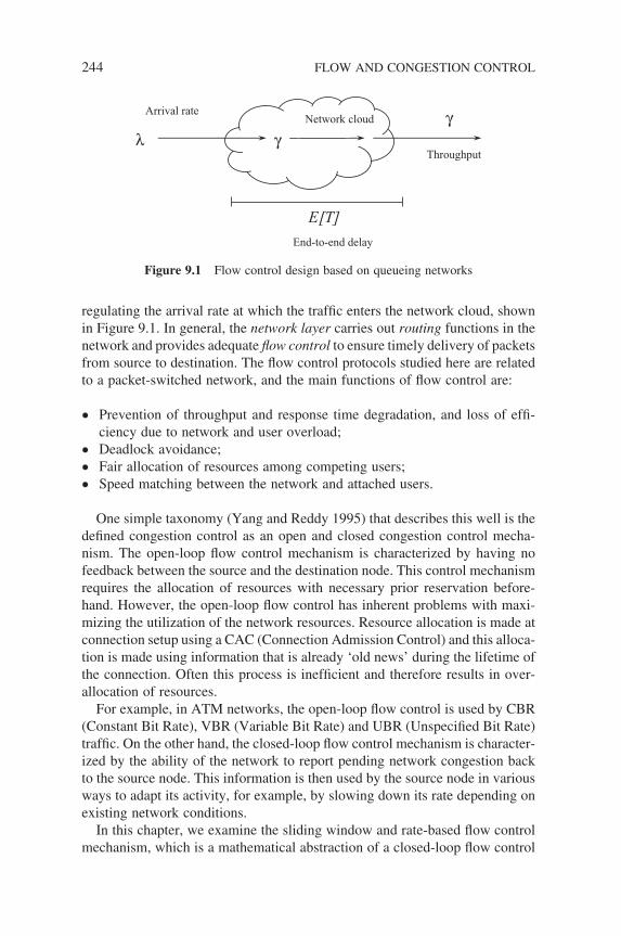
244 FLOW AND CONGESTION CONTROL
regulating the arrival rate at which the traffi c enters the network cloud, shown in Figure 9.1. In general, the network layer carries out routing functions in the network and provides adequate fl ow control to ensure timely delivery of packets from source to destination. The fl ow control protocols studied here are related to a packet-switched network, and the main functions of fl ow control are:
• Prevention of throughput and response time degradation, and loss of effi -ciency due to network and user overload;
• Deadlock avoidance;
• Fair allocation of resources among competing users;
• Speed matching between the network and attached users.
One simple taxonomy (Yang and Reddy 1995) that describes this well is the defi ned congestion control as an open and closed congestion control mecha-nism. The open-loop fl ow control mechanism is characterized by having no feedback between the source and the destination node. This control mechanism requires the allocation of resources with necessary prior reservation before-hand. However, the open-loop fl ow control has inherent problems with maxi-mizing the utilization of the network resources. Resource allocation is made at connection setup using a CAC (Connection Admission Control) and this alloca-tion is made using information that is already ‘old news’ during the lifetime of the connection. Often this process is ineffi cient and therefore results in over-allocation of resources.
For example, in ATM networks, the open-loop fl ow control is used by CBR (Constant Bit Rate), VBR (Variable Bit Rate) and UBR (Unspecifi ed Bit Rate) traffi c. On the other hand, the closed-loop fl ow control mechanism is character-ized by the ability of the network to report pending network congestion back to the source node. This information is then used by the source node in various ways to adapt its activity, for example, by slowing down its rate depending on existing network conditions.
In this chapter, we examine the sliding window and rate-based fl ow control mechanism, which is a mathematical abstraction of a closed-loop fl ow control
End-to-end delay
Arrival rate
Throughput
γγ
E[T]
λ Network cloud
Figure 9.1 Flow control design based on queueing networks
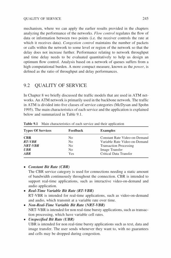
mechanism, where we can apply the earlier results provided in the chapters analyzing the performance of the networks. Flow control regulates the fl ow of data or information between two points (i.e. the receiver controls the rate at which it receives data). Congestion control maintains the number of packets or calls within the network to some level or region of the network so that the delay does not increase further. Performance relating to network throughput and time delay needs to be evaluated quantitatively to help us design an optimum fl ow control. Analysis based on a network of queues suffers from a high computational burden. A more compact measure, known as the power, is defi ned as the ratio of throughput and delay performances.
9.2 QUALITY OF SERVICE
In Chapter 8 we briefl y discussed the traffi c models that are used in ATM net-works. An ATM network is primarily used in the backbone network. The traffi c in ATM is divided into fi ve classes of service categories (McDysan and Spohn 1995). The main characteristics of each service and the application is explained below and summarized in Table 9.1.
Table 9.1 Main characteristics of each service and their application
Types Of Services Feedback Examples
CBR No Constant Rate Video-on-DemandRT-VBR No Variable Rate Video-on-DemandNRT-VBR No Transaction ProcessingUBR No Image TransferABR Yes Critical Data Transfer
QUALITY OF SERVICE 245
• Constant Bit Rate (CBR) The CBR service category is used for connections needing a static amount
of bandwidth continuously throughout the connection. CBR is intended to support real-time applications, such as interactive video-on-demand and audio application.
• Real-Time Variable Bit Rate (RT-VBR) RT-VBR is intended for real-time applications, such as video-on-demand
and audio, which transmit at a variable rate over time.
• Non-Real-Time Variable Bit Rate (NRT-VBR) NRT-VBR is intended for non real-time bursty applications, such as transac-
tion processing, which have variable cell rates.
• Unspecifi ed Bit Rate (UBR) UBR is intended for non real-time bursty applications such as text, data and
image transfer. The user sends whenever they want to, with no guarantees and cells may be dropped during congestion.
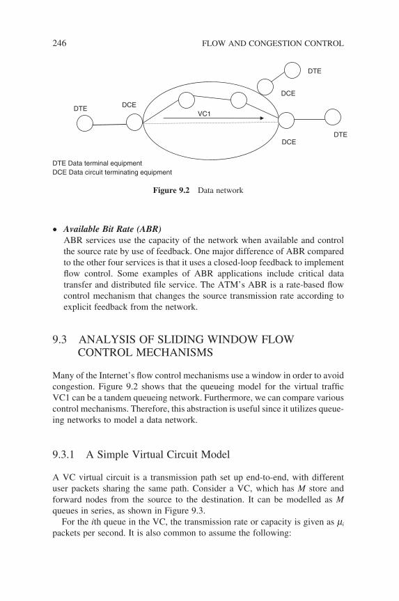
246 FLOW AND CONGESTION CONTROL
• Available Bit Rate (ABR) ABR services use the capacity of the network when available and control
the source rate by use of feedback. One major difference of ABR compared to the other four services is that it uses a closed-loop feedback to implement fl ow control. Some examples of ABR applications include critical data transfer and distributed fi le service. The ATM’s ABR is a rate-based fl ow control mechanism that changes the source transmission rate according to explicit feedback from the network.
9.3 ANALYSIS OF SLIDING WINDOW FLOW CONTROL MECHANISMS
Many of the Internet’s fl ow control mechanisms use a window in order to avoid congestion. Figure 9.2 shows that the queueing model for the virtual traffi c VC1 can be a tandem queueing network. Furthermore, we can compare various control mechanisms. Therefore, this abstraction is useful since it utilizes queue-ing networks to model a data network.
9.3.1 A Simple Virtual Circuit Model
A VC virtual circuit is a transmission path set up end-to-end, with different user packets sharing the same path. Consider a VC, which has M store and forward nodes from the source to the destination. It can be modelled as M queues in series, as shown in Figure 9.3.
For the ith queue in the VC, the transmission rate or capacity is given as mi
packets per second. It is also common to assume the following:
DTE Data terminal equipment DCE Data circuit terminating equipment
DCE
DCE
DCE
DTE
DTE
DTE
VC1
Figure 9.2 Data network
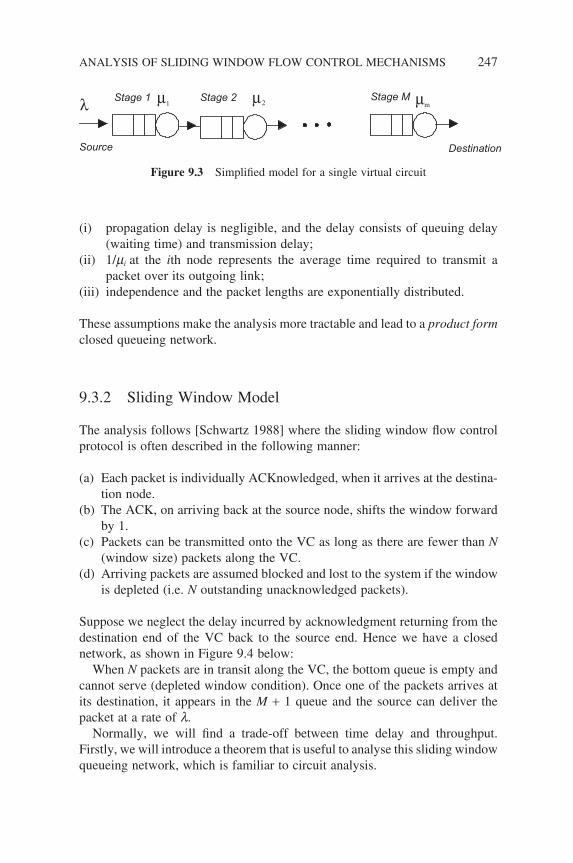
(i) propagation delay is negligible, and the delay consists of queuing delay (waiting time) and transmission delay;
(ii) 1/mi at the ith node represents the average time required to transmit a packet over its outgoing link;
(iii) independence and the packet lengths are exponentially distributed.
These assumptions make the analysis more tractable and lead to a product form closed queueing network.
9.3.2 Sliding Window Model
The analysis follows [Schwartz 1988] where the sliding window fl ow control protocol is often described in the following manner:
(a) Each packet is individually ACKnowledged, when it arrives at the destina-tion node.
(b) The ACK, on arriving back at the source node, shifts the window forward by 1.
(c) Packets can be transmitted onto the VC as long as there are fewer than N (window size) packets along the VC.
(d) Arriving packets are assumed blocked and lost to the system if the window is depleted (i.e. N outstanding unacknowledged packets).
Suppose we neglect the delay incurred by acknowledgment returning from the destination end of the VC back to the source end. Hence we have a closed network, as shown in Figure 9.4 below:
When N packets are in transit along the VC, the bottom queue is empty and cannot serve (depleted window condition). Once one of the packets arrives at its destination, it appears in the M + 1 queue and the source can deliver the packet at a rate of l.
Normally, we will fi nd a trade-off between time delay and throughput. Firstly, we will introduce a theorem that is useful to analyse this sliding window queueing network, which is familiar to circuit analysis.
Stage 1 Stage 2 Stage M
Source Destination
λ µ µ1 2 mµ
Figure 9.3 Simplifi ed model for a single virtual circuit
ANALYSIS OF SLIDING WINDOW FLOW CONTROL MECHANISMS 247
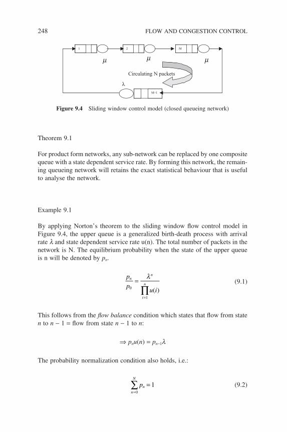
248 FLOW AND CONGESTION CONTROL
Theorem 9.1
For product form networks, any sub-network can be replaced by one composite queue with a state dependent service rate. By forming this network, the remain-ing queueing network will retains the exact statistical behaviour that is useful to analyse the network.
Example 9.1
By applying Norton’s theorem to the sliding window fl ow control model in Figure 9.4, the upper queue is a generalized birth-death process with arrival rate l and state dependent service rate u(n). The total number of packets in the network is N. The equilibrium probability when the state of the upper queue is n will be denoted by pn.
p
pu i
nn
i
n0
1
=
=∏
λ
( ) (9.1)
This follows from the fl ow balance condition which states that fl ow from state n to n − 1 = fl ow from state n − 1 to n:
⇒ pnu(n) = pn−1l
The probability normalization condition also holds, i.e.:
pnn
N
==
∑ 10
(9.2)
m1 M2
M+1
λ
Circulating N packets
mm
Figure 9.4 Sliding window control model (closed queueing network)
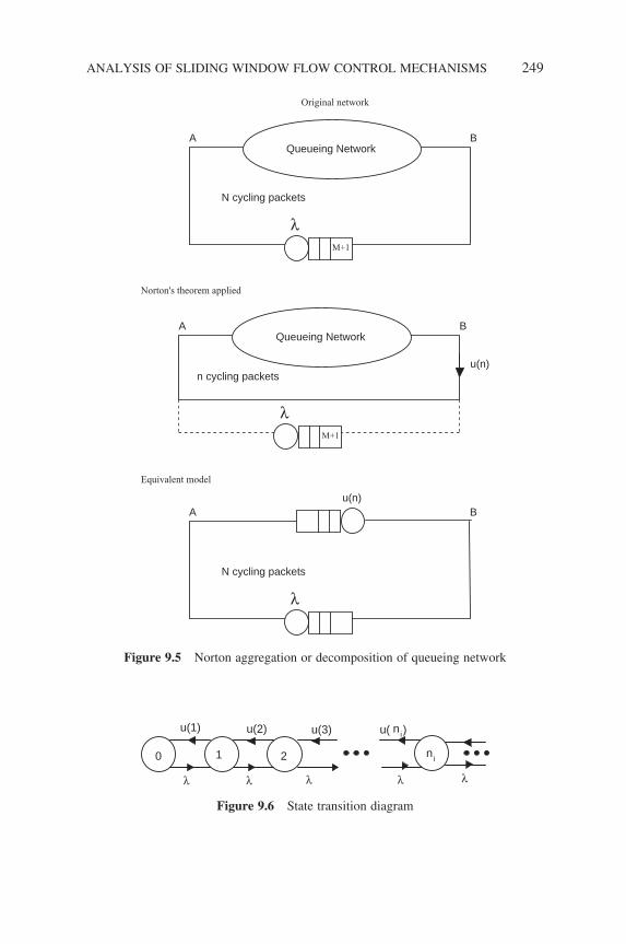
Original network
Queueing Network
N cycling packets
λM+1
BA
Norton's theorem applied
Queueing Network
λM+1
BA
u(n)n cycling packets
Equivalent model
N cycling packets
λ
BAu(n)
Figure 9.5 Norton aggregation or decomposition of queueing network
λ λ λ λ
ni
0 1 2 ni
λ
u(1) u(2) u(3) u( )
Figure 9.6 State transition diagram
ANALYSIS OF SLIDING WINDOW FLOW CONTROL MECHANISMS 249
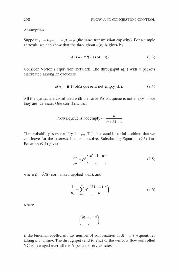
250 FLOW AND CONGESTION CONTROL
Assumption
Suppose m1 = m2 = . . . = mm = m (the same transmission capacity). For a simple network, we can show that the throughput u(n) is given by
u n n n M( ) /( ( ))= + −µ 1 (9.3)
Consider Norton’s equivalent network. The throughput u(n) with n packets distributed among M queues is
u n( ) ( )= ⋅ ≤µ µProb a queue is not empty (9.4)
All the queues are distributed with the same Prob(a queue is not empty) since they are identical. One can show that
Prob a queue is not empty( ) =+ −
n
n M 1
The probability is essentially 1 − p0. This is a combinatorial problem that we can leave for the interested reader to solve. Substituting Equation (9.3) into Equation (9.1) gives
p
p
M n
nn n
0
1=
− +
ρ (9.5)
where r = l/m (normalized applied load), and
1 1
0 0p
M n
nn
n
N
=− +
=
∑ρ (9.6)
where
M n
n
− +
1
is the binomial coeffi cient, i.e. number of combination of M − 1 + n quantities taking n at a time. The throughput (end-to-end) of the window fl ow controlled VC is averaged over all the N possible service rates:
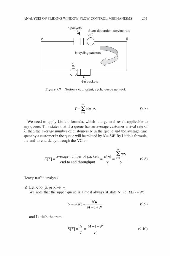
γ ==
∑u n pnn
N
( )1
(9.7)
We need to apply Little’s formula, which is a general result applicable to any queue. This states that if a queue has an average customer arrival rate of l, then the average number of customers N in the queue and the average time spent by a customer in the queue will be related by N = lW. By Little’s formula, the end-to-end delay through the VC is
E TE n
npnn[ ]
[ ]= = = =average number of packets
end to end throughput γ1
NN
∑γ
(9.8)
Heavy traffi c analysis
(i) Let l >> m, or l → ∞We note that the upper queue is almost always at state N, i.e. E(n) ≈ N:
γ µ= =
− +u N
N
M N( )
1 (9.9)
and Little’s theorem:
E TN M N
[ ] = =− +
γ µ1
(9.10)
Figure 9.7 Norton’s equivalent, cyclic queue network
ANALYSIS OF SLIDING WINDOW FLOW CONTROL MECHANISMS 251
N cycling packets
λ
BAu(n)State dependent service rate
n packets
N-n packets
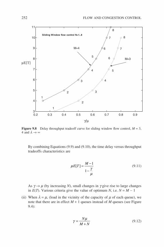
252 FLOW AND CONGESTION CONTROL
By combining Equations (9.9) and (9.10), the time delay versus throughput tradeoffs characteristics are
µ γµ
E TM
[ ] =−
−
1
1 (9.11)
As g → m (by increasing N), small changes in g give rise to large changes in E(T). Various criteria give the value of optimum N, i.e. N = M − 1
(ii) When l = m, (load in the vicinity of the capacity of m of each queue), we note that there are in effect M + 1 queues instead of M queues (see Figure 9.4):
γ µ=
+N
M N (9.12)
0.2 0.3 0.4 0.5
γ/µ
0.6 0.7 0.8 0.93
4
5
6
7
8
9
10
11
M=3
M=4
8
7
6
5
4
3
2
1
8
7
6
5
4
3
2
1
Sliding Window flow control N=1..8
µE[T]
Figure 9.8 Delay throughput tradeoff curve for sliding window fl ow control, M = 3, 4 and l → ∞
and the new time delay expression:
µE TM
MM N
ified to account for M queues
[ ] ( )
mod
=+
+
+
11
(9.13)
The new optimum value of N is
N = M
For the closed queuing network, the product form solution for this type of network is
pg N M
i
i
n
i
M i
( )( , )
n =
=
∏1
1
λµ
(9.14)
g(N, M) is called the normalization constant (statistical parameter of interest). Note that only ‘relative’ values of li can be found and so ri = li/mi no longer represents the actual utilization of the ith queue.
Buzen’s Algorithm (Convolution)
g n m g n m g n mm( , ) ( , ) ( , )= − + −1 1ρ (9.15)
with initial starting condition:
g n n Nn( , ) , , , . . . ,1 0 1 21= =ρ (9.16)
g m m M( , ) , , . . . ,0 1 1 2= = (9.17)
where
ρ λµm
m
m
=
The important desired statistics is contained in the g(N, M) normalization constant. g(N, M) is also related to the moment generating function. Consider the number of packets in queueing station i to be equal to or exceed k packets. Then
Prob /( ) ( , ) ( , )n k g N k M g N Mi ik≥ = −ρ (9.18)
ANALYSIS OF SLIDING WINDOW FLOW CONTROL MECHANISMS 253
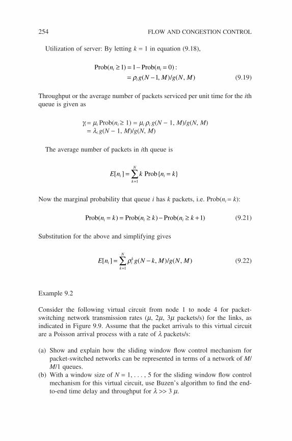
254 FLOW AND CONGESTION CONTROL
Utilization of server: By letting k = 1 in equation (9.18),
Prob Prob
/
( ) ( ) :
( , ) ( , )
n n
g N M g N Mi i
i
≥ = − == −
1 1 0
1ρ (9.19)
Throughput or the average number of packets serviced per unit time for the ith queue is given as
gi = mi Prob(ni ≥ 1) = mi ri g(N − 1, M)/g(N, M)= li g(N − 1, M)/g(N, M)
The average number of packets in ith queue is
E n k n ki ik
N
[ ] = ==
∑ Prob1
Now the marginal probability that queue i has k packets, i.e. Prob(ni = k):
Prob Prob Prob( ) ( ) ( )n k n k n ki i i= = ≥ − ≥ +1 (9.21)
Substitution for the above and simplifying gives
E n g N k M g N Mi ik
k
N
[ ] ( , ) ( , )= −=
∑ρ /1
(9.22)
Example 9.2
Consider the following virtual circuit from node 1 to node 4 for packet-switching network transmission rates (m, 2m, 3m packets/s) for the links, as indicated in Figure 9.9. Assume that the packet arrivals to this virtual circuit are a Poisson arrival process with a rate of l packets/s:
(a) Show and explain how the sliding window fl ow control mechanism for packet-switched networks can be represented in terms of a network of M/M/1 queues.
(b) With a window size of N = 1, . . . , 5 for the sliding window fl ow control mechanism for this virtual circuit, use Buzen’s algorithm to fi nd the end-to-end time delay and throughput for l >> 3 m.
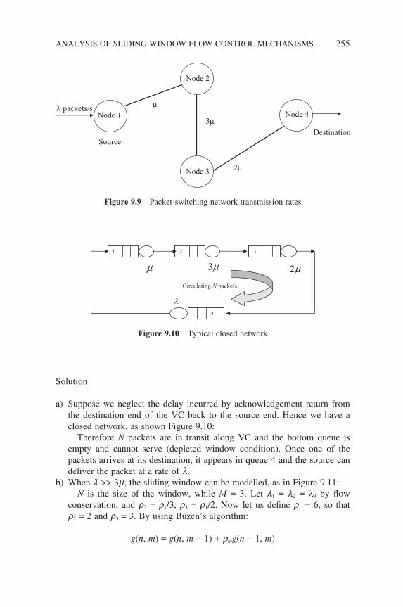
Solution
a) Suppose we neglect the delay incurred by acknowledgement return from the destination end of the VC back to the source end. Hence we have a closed network, as shown Figure 9.10:
Therefore N packets are in transit along VC and the bottom queue is empty and cannot serve (depleted window condition). Once one of the packets arrives at its destination, it appears in queue 4 and the source can deliver the packet at a rate of l.
b) When l >> 3m, the sliding window can be modelled, as in Figure 9.11:N is the size of the window, while M = 3. Let l1 = l2 = l3 by fl ow
conservation, and r2 = r1/3, r3 = r1/2. Now let us defi ne r1 = 6, so that r2 = 2 and r3 = 3. By using Buzen’s algorithm:
g(n, m) = g(n, m − 1) + rmg(n − 1, m)
2µ
λ packets/s
3µ
µNode 1
Node 2
Node 3
Node 4
Destination Source
Figure 9.9 Packet-switching network transmission rates
3µ
1 32
4
λ
Circulating N packets
2µµ
Figure 9.10 Typical closed network
ANALYSIS OF SLIDING WINDOW FLOW CONTROL MECHANISMS 255
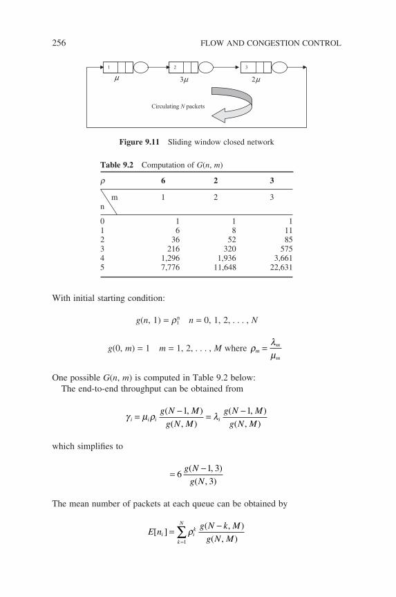
256 FLOW AND CONGESTION CONTROL
With initial starting condition:
g(n, 1) = r1n n = 0, 1, 2, . . . , N
g(0, m) = 1 m = 1, 2, . . . , M where ρ λµm
m
m
=
One possible G(n, m) is computed in Table 9.2 below:The end-to-end throughput can be obtained from
γ µ ρ λi i i ig N M
g N M
g N M
g N M=
−=
−( , )
( , )
( , )
( , )
1 1
which simplifi es to
=−
61 3
3
g N
g N
( , )
( , )
The mean number of packets at each queue can be obtained by
E ng N k M
g N Mi i
k
k
N
[ ]( , )
( , )=
−
=∑ρ
1
1 32
µ3µ
Circulating N packets
µ2
Figure 9.11 Sliding window closed network
Table 9.2 Computation of G(n, m)
r 6 2 3
mn
1 2 3
0 1 1 11 6 8 112 36 52 853 216 320 5754 1,296 1,936 3,6615 7,776 11,648 22,631
The delay over each of the virtual circuits can be determined by Little’s formula:
T TE n
g N k g N
ii
Mi
i
ik
k
N
i
i
= = =−
=
==
=∑
∑∑∑
1
11
3
1
33 3
[ ]( , ) ( , )
γ
ρ
γ
/
When l >> 3m, it is obvious that it is not necessary to calculate the numerator term as it is
E[n] = N
the window size. So the normalized end-to-end throughput and delay can be calculated as a function of the different window size N, as shown in Table 9.3:
9.4 RATE BASED ADAPTIVE CONGESTION CONTROL
For the ATM network, the ABR service will systematically and dynamically allocate available bandwidths to users by controlling the rate of offered traffi c through feedback. The aim of the ABR service is to support applications with vague requirements for throughput and delay. Due to these vague requirements, they are best expressed as ranges of acceptable values. The ABR service allows a user to specify the lower and upper bound on the bandwidth allotted upon connection. The control mechanism is based on feedback from the network to the traffi c source.
The ability for the ABR service to work in a variety of environments, i.e. LANs, MANs or WANs, is particularly important when traffi c is controlled using feedback. The motivation for feedback congestion control is based on adaptive control theory. A simple model may be derived to control the source rate l(t) to optimize a particular objective, such as the throughput or stability. By providing information regarding the buffer occupancy of the bottleneck queue, we can adjust the rate accordingly. The reader is advised to refer to advanced textbooks on the subject, such as (McDysan 2000).
Table 9.3 Normalized end-to-end throughput and delay
N 1 2 3 4 5
g /m 0.545 0.776 0.887 0.942 0.971mT 1.834 2.577 3.382 4.246 5.149
RATE BASED ADAPTIVE CONGESTION CONTROL 257

References
Allen, A.O. Probability, Statistics and Queueing Theory. Academic Press Inc., 1978.Anurag K.D. and Manjunath, J.K. Communication Networking: An Analytical Approach.
Morgan Kaufmann Publishers, 2004.Anick, D., Mitra D. and Sondhi, M.M. ‘Stochastic Theory of a Data-Handling System
with Multiple Sources’. Bell Technical Journal 61(8): 1982.Bae, J.J, et al., ‘Analysis of Individual Packet Loss in a Finite Buffer Queue with Het-
erogeneous Markov Modulated Arrival Processes: A Study of Traffi c Burstiness and Priority Packet Discarding’. INFOCOM ’92, 219–230, 1992.
Baskett, F., Chandy, K.M., Muntz R.R. and Palacios-Gomez, F. ‘Open, Closed and Mixed Networks of Queues with Different Classes of Customers’. Journal of the ACM 22(2): 248–260, 1975.
Bertsekas, D and Gallager, R. Data Networks, 2nd Edition. Prentice-Hall International Inc., 1992.
Blondia, C. and Casals, O. ‘Statistical Multiplexing of VBR Sources: A Matrix-Analysis Approach’. Performance Evaluation 16: 5–20, 1992.
Bolch, G., Greiner, S., de Meer, H. and Trivedi, K.S. Queueing Networks and Markov Chains. Wiley Interscience. 2006.
le Boudec, J-Y. and Thiran. P. Network Calculus. Springer Verlag, 2002.Bruell, S.C. and Balbo, G. Computational Algorithms for Closed Queueing Networks.
North-Holland, 1980.Bruneel, H. ‘Queueing Behavior of Statistical Multiplexers with Correlated Inputs’.
IEEE Trans. Commmunications, 36: 1339–1341, 1988.Bruneel, H. and Byung G.K. Discrete-Time Models for Communication Systems Includ-
ing ATM. Kluwer Academic Publishers, 1993.Burke, P.J. ‘The Output of a Queueing System’. Operations Research 4(6): 699–704,
1956.Buzen, J.P. ‘Computational Algorithms for Closed Queueing Networks with Exponen-
tial Servers’. ACM 16(9): 527–531, 1973.
Queueing Modelling Fundamentals Second Edition Ng Chee-Hock and Soong Boon-Hee© 2008 John Wiley & Sons, Ltd
260 REFERENCES
Buzen, J.P. ‘Operational Analysis: The Key to the New Generation of Performance Prediction Tools’. Proceedings of the IEEE Compcon, September 1976.
N. Cardwell, Savage, S. and Anderson, T. ‘Modelling TCP Latency’ Proceedings of the IEEE Infocom, 2000.
Chao, H.J. and Guo, X. Quality of Service Control in High-Speed Networks, 2002.Chandy, K.M., Hergoy, U. and Woo, L. ‘Parametric Analysis of Queueing Network
Models’. IBM Journal of R&D, 19(1): 36–42, 1975.Chang, C-S. Performance Guarantees in Communication Networks. Springer Verlag,
2000.Chen, J.S.-C., Guerin, R. and Stern, T.E. ‘Markov-Modulated Flow Model for the Output
Queues of a Packet Switch’. IEEE Trans. Communications. 40(6): 1098–1110, 1992.Chen, H. and Yao, D.D. Fundamentals of Queueing Networks, Springer-Verlag, 2001.Cinlar, E. Introduction to Stochastic Processes. Prentice-Hall, 1975.Cohen, J.W. The Single Serve Queue. North-Holland, 1982.Diagle, J.N. and Langford, J.D. ‘Models for Analysis of Packet Voice Comunications
Systems’. IEEE Journal Sel Areas Communications SAC-4(6): 1986.Denning, P.J. and Buxen, J.P. ‘The Operational Analysis of Queueing Network Models’.
Computer Surveys 10(3): 1978.Elwalid, A.I., Mitra, D. and Stern, T.E. ‘Statistical Multiplexing of Markov Modulated
Sources Theory and Computational Algorithms’. ITC-13, 495–500, 1991.Elwalid, A.I. and Mitra, D. ‘Fluid Models For The Analysis and Design of Statistical
Multiplexing With Loss Priority On Multiple Classes of Bursty Traffi c’. IEEE INFOCOM ’92, 415–425, 1992.
Feller, W. An Introduction to Probability Theory and Its Applications, 3rd Edition,Volume I. John Wiley and Sons, 1968.
Firoiu, V. et al. ‘Theory and Models for Internet Quality of Service’. Proceedings of the IEEE, May 2002.
Fischer, W. and Meier-Hellstern, K. ‘The Markov-modulated Poisson Process (MMPP) Cookbook’. Performance Evaluation 18: 147–171, 1993.
Fortz, B. and Thorup, M. ‘Internet Traffi c Engineering by Optimizing OSPF Weights’. IEEE INFOCOM 2000, 2000.
Frost, V.S. and Melamed, B. ‘Traffi c Modelling for Telecommunications Networks’. IEEE Communications Magazine, 70–81, 1994.
le Gall, D. ‘MPEG: A Video Compression Standard for Multimedia Applications’. Com-munications of the ACM 34(4): 47–58, 1991.
Gebali, F. Computer Communication Networks Analysis and Design, Northstar Digital Design Inc, Victoria, BC 2005.
Gelenbe, E. and Pujolle, G. Introduction to Queueing Networks. John Wiley & Sons, 1987.
Gerla, M. and Kleinrock, L. ‘Flow Control: A Comparative Survey.’ IEEE Trans. on Communications 28(4): 553–574, 1980.
Ghanbari, M, and Hughes, C.J. ‘Packing Coded Video Signals into ATM Cells’. IEE/ACM Trans. on Networking 1(5): 505–509, 1993.
Giambene, G. Queueing Theory and Telecommunications. Springer-Verlag, 2005.Gordon, W.J and Newell, G.F. ‘Closed Queueing Systems With Exponential Servers’.
Operations Research 15(2): 254–265, 1967.Gross, D and Harris, C.M. Fundamentals of Queueing Theory. John Wiley & Sons:
New York, 1974.
REFERENCES 261
Gunter, B., Greiner, S., de Meer, H., Trivedi, K.S. Queueing Networks and Markov Chains. John Wiley & Sons, 2006.
Habib, I.W. and Saadawi, T.N. ‘Multimedia Traffi c Characteristics in Broadband Net-works’. IEEE Communications Magazine 48–54, July 1992.
Haight, F.A. Applied Probability. Plenum Press: New York and London, 1981.Harrison, P.G. and Patel, N.M. Performance Modelling of Communication Networks
and Computer Architectures. Addison-Wesley Publishing Company, 1993.Hayes, J.F. Modeling and Analysis of Computer Communications Networks. Plenum
Press: New York and London, 1984.Heffes, H. and Lucantoni, D.M. ‘A Markov Modulated Characterization of Packetized
Voice and Data Traffi c and Related Statistical Multiplexer Performance’. IEEE Journal of Sel Areas in Communications SAC-4(6): 1986.
Horn, R.A. and Johson, C.R.. Matrix Analysis. Cambridge University Press, 1990.Jackson, J.R. ‘Networks of Waiting Lines’. Operations Research 5(4): 518–521,
1957.Jackson, J.R. ‘Jobshop-Like Queueing Systems’. Management Science 10(1): 131–142,
1963.Jain, J.L., Mohanty, S.G. and Bohm, W. A Course on Queueing Models. Chapman &
Hall, 2006.Jaiswal, J.M. Priority Queues. Academic Press, 1968.King, P J.B. Computer and Communication Systems Performance Modelling. Prentice-
Hall, 1990.Kleinrock, L. Communication Nets: Stochastic Message Flow and Delay. McGraw Hill:
New York 1964, reprinted by Dover: New York 1972.Kleinrock, L. Queueing Systems, Volume. 1. John Wiley & Sons: New York, 1975.Kleinrock, L. ‘Performance Evaluation of Distributed Computer-Communication
Systems’. In: Queueing Theory and Its Applications (Boxma, O.J. and Syski, R. eds), North-Holland, 1988.
Kobayashi, H. Modeling and Analysis: An Introduction to System Performance Evalu-ation Methodology. Addison-Wesley 1978.
Lavenberg, S.S. and Reiser, M. ‘Stationary State Probabilities at Arrival Instants of Closed Queueing Networks with Multiple Types of Customers’. Journal of Applied Probability 19: 1048–1061, 1980.
Lee, Hyong W. and Mark, J.W. ‘ATM Network Traffi c Characterization Using Two Types of On-Off Sources’ IEEE INFOCOM ’93: 152–159, 1993.
Leduc, J-P. Digital Moving Pictures Coding and Transmission on ATM. Elsevier, 1994.
Li, S-Q. ‘A General Solution Technique for Discrete Queueing Analysis of Multimedia Traffi c on ATM’. IEEE Trans. Communications 39: 115–1132, 1991.
Little, J. ‘A Proof of the Queueing Formula L = lW’. Operations Research 18: 172–174, 1961.
Lucantoni, D.M., Meier-Hellstern, K.S. and Neuts, M.F. ‘A Single Server Queue with Server Vacations and a Class of Non-renewal Arrival Process’. Advances in Applied Probability 22(2): 676–705, 1990.
Luhanga, M.L. ‘A Fluid Approximation Model of an Integrated Packet Voice and Data Multiplexer’. Proc of INFOCOM ’88, 687–692, 1988.
Magnus, J.R. and Neudecker, H. Matrix Differential Calculus with Applications in Statistics and Econometrices. John Wiley & Sons, 1988.
262 REFERENCES
Martin, J. Design of Real-Time Computer Systems. Prentice Hall, 1967.McDysan, D.E. and Spohn, D.L. ATM: Theory and Application. McGraw-Hill, 1995.McDysan D.E., QoS and Traffi c Management in IP & ATM Network. McGraw Hill,
2000.Neuts, M.F. Matrix-Geometric Solutions in Stochastic Models. The John Hopkins Uni-
versity Press, 1981.Neuts, M.F. Structured Stochastic Matrices of M/G/1 Type and Their Applications.
Marcel Dekker, Inc., 1989.Newman, P. ‘ATM Technology for Corporate Networks’. IEEE Communications Maga-
zine, 90–101, April 1992.Nomura, M., et al. ‘Basic Characteristics of Variable Rate Video Coding in ATM Envi-
ronment’. IEEE Journal Sel. in Communications 7(5): 752–760, 1989.Mieghem, P.V. Performance of Communications Networks and Systems. Cambridge
University Press, 2006.Onvural, R.O. Asynchronous Transfer Mode Networks Performance Issues. Artech
House, Inc., 1994.Papoulis, A. Probability, Random Variables, and Stochastic Processes, 3rd Edition.
McGraw-Hill, 1991.Prabhu, N.U. and Zhu, Y. ‘Markov-Modulated Queueing Systems’. Queueing Systems
5: 215–246, 1989.Ramamurthy, G. and Sengupta, B. ‘Modeling and Analysis of a Variable Bit Rate Video
Multiplexer’. INFOCOM ’92 817–827, 1992.Reiser, M. and Kobayashi, H. ‘Numerical Solution of Semiclosed Exponential Server
Queueing Networks’. Proceedings of the 7th Asilomar Conference on Circuits Systems and Computers, 308–312. November 1973.
Reiser, M. ‘A Queueing Network Analysis of Computer Communication Networks with Window Flow Control’. IEEE Trans. on Communications, 27(8): 1990–1209, 1979.
Reiser, M. and Lavenberg, S.S. Mean Value Analysis of Closed Multichain Queueing Networks’. Journal of the ACM 22: 313–322, 1980.
Reiser, M. ‘Performance Evaluation of Data Communication Systems’. Proceedings of the IEEE 70(2): 171–195, 1982.
Ren, Q. and Kobayashi, H. ‘Diffusion Process Approximations of a Statistical Multi-plexer with Markov Modulated Bursty Traffi c Sources’. GLBECOM ’94 3: 1100–1106, 1994.
Robertazzi, T.G. Computer Networks and System: Queueing Theory and Performance Evaluation, 3rd Edition, Springer-Verlag, 2000.
Robertazzi, T.G. Planning Telecomunication Networks. IEEE: Piscataway, NJ. 1999.Ross, S.M. Stochastic Processes. John Wiley & Sons, 1983.Sen, P., et al. ‘Models for Packet Switching of Variable-Bit-Rate Video Sources’. IEEE
Journal of Sel Areas Communications 7(5): 865–869, 1989.Schwartz, M. Telecommunication Networks Protocol, Modeling and Analysis. Addison-
Wesley, 1987.Schwartz, M. Broadband Integrated Networks. Prentice Hall, 1996.Sevcik, K.C. and Mitrani I. ‘The Distribution of Queueing Network States at Input and
Output Instants’. Journal of the ACM 28(2): 358–371, 1981.Skelly, P.M., Schwartz, M. and Dixit, S. ‘A Histogram-Based Model for Video Traffi c
Behavior in an ATM Multiplexer’. IEEE/ACM Trans. on Networking 1(4): 446–459, 1993.
REFERENCES 263
Spragin, J.D., Hammond, J.L. and Pawlikowski, K. Telecommunications: Protocol and Design. Addison-Wesley: Reading, MA., 1991.
Sohraby, K. ‘On the Asymptotic Behavior of Heterogeneous Statistical Multiplexer With Applications’. INFOCOM ’92 839–847, 1992.
Sriram, K. and Whitt, W. ‘Characterizing Superposition Arrival Processes in Packet Multiplexers for Voice and Data’. IEEE Journal of Sel. Area Communications SAC-4(6): 833–845, 1986.
Taylor, H.M. and Karlin, S. An Introduction To Stochastic Modeling. Academic Press, 1994.
Tian, N. and Zhe, G.Z. Vacation Queueing Models: Theory and Applications. Springer-Verlag, 2006.
Tijms, H.C. Stochastic Models: An Algorithmic Approach. John Wiley & Sons, 1994.Van Dijk, N. Queueing Networks and Product Forms A Systems Approach. John Wiley
& Sons, 1993.Vesilo, R.A.. ‘Long-Range Dependence of Markov Renewal Processes’. Australian and
New Zealand Journal of Statistics 46(1): 155–171, 2004.Wolff, R.W. ‘Poisson Arrivals See Time Averages’. Operations Research 30: 223–231,
1982.Wright, S. ‘Admission Control in Multi-service IP Networks: A Tutorial’. IEEE Com-
munications Surveys and Tutorials, July 2007.Xiong, Y. and Bruneel, H. ‘A Tight Upper Bound for the Tail Distribution of the Buffer
Contents in Statistical Multiplexers with Heterogeneous MMBP Traffi c Sources’. GLOBECOM ’93 767–771, 1993.
Yang, C. and Reddy, A. ‘A Taxonomy for Congestion Control Algorithms in Packet Switching Network’, IEEE Networks, July/August 1995.
Ye, J. and Li, S-Q. ‘Analysis of Multi-Media Traffi c Queues with Finite Buffer and Overload Control – Part I: Algorithm’. INFOCOM ’91, 464–1474, 1991.
Ye, J. and Li, S-Q. ‘Analysis of Multi-Media Traffi c Queues with Finite Buffer and Overload Control – Part II: Applications’. INFOCOM ’92, 1464–1474, 1992.


Index
Note: page numbers in italics refer to fi gures and diagrams
Queueing Modelling Fundamentals Second Edition Ng Chee-Hock and Soong Boon-Hee© 2008 John Wiley & Sons, Ltd
ABR (available bit rate) 246, 257arrival curve 239–40arrival process, Markov-modulated
217–42arriving population, size of 45asynchronous transfer mode see
ATMATM (Asynchronous Transfer Mode)
networks 135, 217, 257applications of fl uid fl ow model to
236service categories of traffi c 245–6
available bit rate see ABRaverage value 13axiom of probability 9
balance equations 190–3Bayes’ formula 6Bernoulli random variable 10Bernoulli trial 10, 59–60
sample sequence 75binomial distribution 25, 59–60binomial random variable 10, 14birth-death processes 96–100
transition diagram 96blocked-calls telephone system 135blocking probability 119–20, 119Boudec, Jean-Yves 218broadband integrated services networks
217
Burke’s theorem 176–8Buzen’s algorithm (convolution) 253
CAC (connection admission control) 244
Cauchy random variable 15CBR (constant bit rate) 244, 245Central limit theorem 22central server system 213Chapman–Kolmogorov forward
equations 80circuit-switching data networks 170closed network, typical 255closed queueing networks 51, 169, 171,
197–215applications of 213–14examples 171, 201Jackson closed queueing networks
197–9performance measures 207–10
closed serial network 206conditional probability 5
and independence 5–7congestion control 243–57connection admission control see CACconstant bit rate see CBRcontinuous random variable 8, 12continuous-state process 72continuous time Markov chains 91–5continuous (time) – parameter process 73
266 INDEX
continuous uniform random variable 11convolution algorithm 203–7convolution property
of Laplace transforms 29of z-transforms 23–4
CPU job scheduling problems 171CPU system 50–1Cruz, Rene L. 236cumulative probability distribution
function 8customer arriving pattern (A) 50
data exchange sequence 154, 154data network 246decomposition property 63–4delay probability 126density function 21detailed balance equation 107deterministic distribution (D) 46differentiation property of Laplace
transform 30Dirac delta function 113discrete and continuous Markov
processes 71–102discrete random variables 8, 12, 13discrete-state process 72discrete time Markov chains 74–91
defi nition 75–8sojourn times 90–1
discrete (time) – parameter process 73distribution function 8
of continuous RV 9of discrete random variable 13joint 16of system state 146–7of system time 147–8
distribution(s)marginal 16and random variables 8–12state probability 93–5
eigenvalues 34–6eigenvectors 34–7Engset’s loss systems 131–3ensemble (or stochastic) average 53, 56ergodocity 55Erlang, A.K. 43, 135Erlang B formula 130
Erlang distribution (Ek) 46Erlang-k random variable 12Erlang’s loss formula 130Erlang’s loss queueing systems – M/M/
m/m systems 129–31expectation property of Laplace
transform 29expected values and variances 13–15exponential random variable 11, 30, 64exponentially distributed inter-arrival
times 64
FCFS (fi rst-come-fi rst-served) 47–8, 111, 142
feedback loops 169feedback open network 172Fibonacci numbers 32fi rst-come-fi rst-served see FCFSfl ow and congestion control 243–57
quality of service 245–6fl ow balance 248fl ow conservation law 57–9, 57, 58, 170fl ow control 243–7
design based on queueing networks 244
G/M/1 queueing system 141, 165–7G1/M/1 queueing system 166
performance measures 166–7Gamma random variable 11, 35Gaussian (Normal) random variable 12general and independent (inter-arrival
time) distribution 46general probability distribution 46general service times distribution (G) 48general transient solutions for state
probabilities 81–6generating functions 22–8gometric distribution 25geometric random variable 10global balance concept 106–7, 106global balance equation 106, 189
imbedded Markov chain approach 142–3, 142
independenceand conditional probability 5–7of random variables 21–2
INDEX 267
index parameter 72–3infi nitesimal generator 94input process characteristics 45–6
arriving pattern 45–6behaviour of arriving customers 46size of arriving population 45
inter-arrival time distribution 46Internet fl ow control mechanisms 246
Jackson closed queueing networks 197–9
Jackson queueing networks 181–6job processing 169
system 50–1, 50joint density function 16joint distribution function 16joint probability mass function 17joint random variables and their
distributions 16–21
k-stage Erlang random variable 12, 30, 31
Kendall, David G. 50Kendall notation 50–1Kirchhoff’s current law 57Kleinrock independence assumption 21,
179
Laplace, Pierre Simon Marquis De 28Laplace transforms 20, 28–32
pairs 35for probability functions 31properties 29–32
convolution 29differentiation 30expectation 29linearity 29uniqueness 29
last-come-fi rst-served see LCFSLaw of Total Probability 6LCFS (last-come-fi rst-served) 47–8linearity property
of Laplace transforms 29of z-transforms 23
Little, J.D.C. 52Little’s theorem (law or result) 52–6
general applications 54–5local balance concept 106–7, 107
local balance equation 107, 190lost-calls-cleared telephone system 135lost-calls-delayed telephone system 135
M/G/1 queueing systems 141, 142–8, 151
analysis of, using imbedded Markov-chain approach 143–6
non-preemptive priority queueing 158–60, 159
performance measures 160–3performance measures 150–5with service vacations 155–8
performance measures 156–8M/M/1 queueing systems 104–10, 104
with fi nite customer population 51number of customers in system 109performance measures 107–10system time (delay) distribution
111–18M/M/1/S queueing systems 118–24
performance measures 120–4transitional-rates diagram 118
M/M/m 125performance measures 126–7transition diagram 125waiting time distribution of M/M/m
127–9M/M/m/m – Erlang’s loss queueing
systems 129–31performance measures 130–1system with fi nite customer population
132performance measures 133–4
transition diagram 132m-state MMPP 225, 226marginal distribution 16Markov chain/process
birth-death processes 96–100continuous time 91–5
defi nition 91–2discrete and continuous 71–102discrete time 74–91imbedded Markov chain approach
142reducibility and periodicity 88–90semi-Markovian queueing systems
141–68
268 INDEX
single-queue 103–40steady-state behaviour 86–8
Markov-modulated arrival process 217–42
Markov-modulated Bernoulli process (MMBP) 217, 227–33
SMMBP/D/1 229–31initial conditions 233queue length solution 231–2source model and defi nition 227superposition of N identical MMBPs
228–9two-state MMBP 227, 227
Markov-modulated fl uid fl ow 217, 233–6
applications to ATM 236model 234
and queue length analysis 233–6Markov-modulated Poisson process
(MMPP) 217, 218, 218–26applications of 226defi nition and model 218–23m-state MMPP 225, 226MMPP/G/1 225, 225–6superposition of MMPPs 223–4, 224
Markovian (memoryless) distribution (M) 46
of Poisson process 64–6sample train arrival 65
Markovian queues in tandem 171, 171–8
analysis of 175–6application in data networks 178–81state transition diagram 173
matrixcalculus 36–8formulation of state probabilities
79–81operations 33–8
mean value 13mean value analysis see MVAmemoryless chain 75min-plus algebra 241–2mixed random variable 12MMBP see Markov-modulated Bernoulli
processMMPP see Markov-modulated Poisson
process
multi-server 124queues 176systems – M/M/M 124–9
MVA (mean value analysis) 210–13
network calculus 218, 236–42arrivals and X(t) content 238input traffi c characterization – arrival
curve 239–40sample arrival curve 240sample path of A(t) and D(t)system characterization – service
curve 240–1system description 237–9system view of queue 237
network layer 244Neuts, Marcel F. 33non-blocking networks 170non-preemptive priority 48
M/G/1 158–60, 159performance rates 160–3
non-real-time variable bit rate see NRT-VBR
Normal (Gaussian) random variable 12
normalization conditions 10normalization constant 253Norton aggregation or decomposition of
queueing network 249Norton’s equivalent, cyclic queue
network 251Norton’s theorem 248NRT (non-real-time variable bit rate)
245
offered load 56one step transitional probability 75open-loop fl ow control 244open queueing networks 169–95
example 170performance measures 186–90
operations research 43output process characteristics 47–8
packet-switching data networks 170packet-switching network transmission
rates 255Paradox of Residual Life 152
INDEX 269
parallel servers 47number of (X) 50
PASTA (Poisson Arrivals See Time Averages) 110–11, 112, 143
PDF (probability distribution function) 8pdf (probability density function) 9, 13,
20, 30performance measures
closed queueing networks 207–10G1/M/1 166–7M/G/1 150–5
non-preemptive priority 160–3with service vacations 156–8
M/M/1 107–10M/M/1/S 120–4M/M/m 126–7M7/M/m/m 130–1open networks 186–90
pmf (probability mass function) 9, 13physical number and layout of servers
46point-to-point setup 153, 153Poisson Arrivals See Time Averages see
PASTAPoisson distribution 25
sample 62Poisson process 45, 59–62
arrival perspective 60–2limiting case 59–60properties 62–9
decomposition 63–4exponentially distributed inter-
arrival times 64memoryless (Markovian), of inter-
arrival times 64–6Poisson arrivals during random time
interval 66–9superposition 62–3, 63
Poisson random variable 10–11, 14Pollaczek-Khinchin formula 150pre-emptive resume priority queueing
48M/G/1 163–5
priority 47–8priority queueing systems 158–65
non-preemptive priority 48M/G/1 158–60, 159performance rates 160–3
preemptive 48, 158M/G/1 163–5
probabilityaxioms of, and sample spaces 2–5conditional, and independence 5–7density 9fl ow 106, 190law of total probability 6theory 1–22
probability density function see pdfprobability distribution, steady-state
199–203probability distribution function see
PDFprobability mass function see pmfproblems
closed queueing networks 214–15discrete and continuous Markov
processes 100–2introduction to queueing systems
69–70open queueing networks 193–5preliminaries 39–40semi-Markovian queueing systems
167–8single-queue Markovian systems
139–40processor sharing 47–8product-form queueing networks 190pure-birth process 97
quality of service (QoS) 243, 245–6queue-by-queue decomposition 176queued-calls telephone system 135queueing discipline (serving discipline)
(Z) 47–8queueing models, considerations for
applications of 134–9queueing networks with blocking 170queueing probability 126queueing system(s)
introduction 43–70nomenclature 44–5random variables 49schematic diagram 44structure characteristics 46–7
queueing theory 43queueing time 109
270 INDEX
random 47random time interval, Poisson arrivals
during 66–9random variable(s) (RV) 8
Bernoulli 10binomial 10continuous 8continuous uniform 11discrete 8and distributions 8–12Erlang-k (k-stage Erlang) 12exponential 11Gamma 11geometric 10independence of 21–2joint, and their distributions 16–21means and variances of 15mixed 12Normal (Gaussian) 12Poisson 10random sum of 18and their relationships 48–9uniform 11
rate based adaptive congestion control 257
real-time variable bit rate see RT-VBRreducibility and periodicity of Markov
chain 88–90residual service time 142, 148–50, 148resource utilization and traffi c intensity
56–7RT-VBR (real-time variable bit rate)
245RV see random variable(s)
sample point 6sample space 6
and axioms of probability 2–5saturation probability 120scalar vector 37semi-Markovian queueing systems
141–68serial servers 47servers
parallel 47physical number and layout of 46serial 47
service curve 240–1
service pattern (service-time distribution (B)) 48, 50
service vacations, M/G/1 with 155–8serving discipline see queueing
disciplineShaolin monks puzzle 26, 26simple feedback open network 172simple virtual circuit model 246–7single-queue Markovian systems 103–40sliding window
analysis of fl ow control mechanisms 246–57
simple virtual circuit model 246–7closed network 256control model (closed queueing
network) 248data link protocol 151model 247–57protocol 247–9
spectral representation 34–6standard deviation 13state space 72state probability
distribution 93–5general transient solutions for 81–6
state transition diagram 76, 76, 88, 98, 249
lift example 77statistical dependency 73–4steady-state behaviour of Markov chain
86–8steady-state probability distribution
199–203stochastic average see ensemble averagestochastic matrix 79stochastic (or probability) fl ow 106stochastic processes 72–4
classifi cations 73discrete-state process 72index parameter 72–3statistical dependency 73–4
stochastic sequence 73Stop-and-Wait data link protocol 151Strong law of large numbers 21superposition property 62–3, 63
of MMPPs 223–4, 224of N identical MMBPs 228–9
system capacity (Y) 46, 50
INDEX 271
system delay 109system state, distribution of 146–7system time 109
distribution of 147–8
tandem queues 171, 171–8analysis of 175–6application in data networks
178–81state transition diagram 173
time-homogeneous Markov chain 75
total probabilitylaw 6theorem 19
traffi c intensity and resource utilization 56–7
transforms 20transition 73, 76transition diagram 76
of birth-death process 96–100M/M/m 125M/M/m/m 132
transition matrix 79transitional probability matrix 79
cf transition-rate matrix 95transitional probability (one step) 75transitional-rates diagrams
M/M/1/S 118transition-rate matrix 95
cf transition-probability matrix 95two-state Markov process 98
UBR (unspecifi ed bit rate) 244, 245uniform random variable 11unspecifi ed bit rate see UBR
variable bit rate see VBRvariance 13
and expected values 13–15VBR (variable bit rate) 244, 245VC see virtual circuitvirtual circuit (VC)
packet switching network 180queueing model for 180simple model 246–7
waiting time 109distribution of M/M/m 127–9
Yule process 99
z-transformation 22z-transforms 22–8
for discrete random variables 26pairs 24properties 23–8
convolution 23–4fi nal values and expectation 24linearity 23