Questions to the UniverseAn introduction to particle and astroparticle physics

Alessandro De Angelis and Mario Pimenta

September 26, 2012

Contents

1 introduction 3

2 The birth and the basics of particle physics 42.1 Atomic models . . . . . . . . . . . . . . . . . . . . . . . . . . . . 42.2 The Rutherford experiment . . . . . . . . . . . . . . . . . . . . . 52.3 Cross-section and interaction length . . . . . . . . . . . . . . . . 7

2.3.1 Total cross-section . . . . . . . . . . . . . . . . . . . . . . 72.3.2 Differential cross-sections . . . . . . . . . . . . . . . . . . 82.3.3 Cross-sections at colliders . . . . . . . . . . . . . . . . . . 92.3.4 Partial cross-sections . . . . . . . . . . . . . . . . . . . . . 92.3.5 Interaction length . . . . . . . . . . . . . . . . . . . . . . 9

2.4 The Fermi golden rule and the Rutherford scattering . . . . . . . 102.5 Particle scattering in static fields . . . . . . . . . . . . . . . . . . 13

2.5.1 Extended charge distributions . . . . . . . . . . . . . . . . 132.5.2 Finite range interactions . . . . . . . . . . . . . . . . . . . 142.5.3 Electron scattering . . . . . . . . . . . . . . . . . . . . . . 15

2.6 Special relativity . . . . . . . . . . . . . . . . . . . . . . . . . . . 152.6.1 Lorentz transformations . . . . . . . . . . . . . . . . . . . 162.6.2 Space-time interval . . . . . . . . . . . . . . . . . . . . . . 172.6.3 Energy and momentum . . . . . . . . . . . . . . . . . . . 182.6.4 Mandelstam variables . . . . . . . . . . . . . . . . . . . . 192.6.5 Lorentz invariant transition rates, phase space, fluxes and

cross-sections . . . . . . . . . . . . . . . . . . . . . . . . . 212.7 Decays . . . . . . . . . . . . . . . . . . . . . . . . . . . . . . . . . 22

2.7.1 β decay and the neutrino hypothesis . . . . . . . . . . . . 242.8 Fields and particles . . . . . . . . . . . . . . . . . . . . . . . . . . 252.9 Units . . . . . . . . . . . . . . . . . . . . . . . . . . . . . . . . . . 26

3 Cosmic rays and the development of the physics of elementaryparticles and fundamental interactions 313.1 The puzzle of atmospheric ionisation and the discovery of cosmic

rays . . . . . . . . . . . . . . . . . . . . . . . . . . . . . . . . . . 323.1.1 Experiments underwater and in height . . . . . . . . . . . 343.1.2 The nature of cosmic rays . . . . . . . . . . . . . . . . . . 38

1

3.2 Cosmic rays and the beginning of particle physics . . . . . . . . . 383.2.1 Relativistic quantum mechanics and antimatter . . . . . . 393.2.2 The discovery of antimatter . . . . . . . . . . . . . . . . . 423.2.3 Cosmic rays and the progress of particle physics . . . . . 433.2.4 The µ lepton and the π mesons . . . . . . . . . . . . . . . 453.2.5 Strange particles . . . . . . . . . . . . . . . . . . . . . . . 483.2.6 Mountain-top laboratories . . . . . . . . . . . . . . . . . . 49

3.3 Particle hunters become farmers . . . . . . . . . . . . . . . . . . 50

4 Particle detection 534.1 Interaction of particles with matter . . . . . . . . . . . . . . . . . 53

4.1.1 Charged particle interactions . . . . . . . . . . . . . . . . 534.1.2 Photon interactions . . . . . . . . . . . . . . . . . . . . . 614.1.3 Nuclear (hadronic) interactions . . . . . . . . . . . . . . . 644.1.4 Range . . . . . . . . . . . . . . . . . . . . . . . . . . . . . 64

4.2 Particle detectors . . . . . . . . . . . . . . . . . . . . . . . . . . . 654.2.1 Track detectors . . . . . . . . . . . . . . . . . . . . . . . . 654.2.2 Photosensors . . . . . . . . . . . . . . . . . . . . . . . . . 734.2.3 Cherenkov detectors . . . . . . . . . . . . . . . . . . . . . 754.2.4 Transition radiation detectors . . . . . . . . . . . . . . . . 764.2.5 Calorimeters . . . . . . . . . . . . . . . . . . . . . . . . . 76

2

Chapter 1

Introduction

3

Chapter 2

The birth and the basics ofparticle physics

2.1 Atomic models

The Universe around us, the objects surrounding us, have an enormous diver-sity. Is this diversity built over small hidden structures? This interrogationstarted to be, as often, a philosophical question, to become, several thousandyears later, a scientific one. In the VI and V century BC in India and Greece theatomic concept was proposed: matter was formed by small invisible, indivisibleand eternal particles - the atoms, a word invented by Leucippus (460 BC) andmade popular by his disciple Democritus. In the late XVIII, early XIX century,Chemistry gave finally to atomism the status of a scientific theory (mass con-servation law - Lavoisier 1789; ideal gas laws - Gay-Lussac 1802; law of partialpressures - Dalton 1805), which was strongly reinforced with the establishmentof the Periodic Table of elements by Mendeleev in 1869 - the chemical propertiesof the elements depends on a “magic” number, their atomic number.

If atoms did exist their shape and structure were to be discovered. ForDalton, who lived before electromagnetism, atoms had to be able to establishmechanical links with each other. After Maxwell (the electromagnetic fieldequations) and Thompson (the electron) the binding force was the electric oneand in atoms an equal number of positive and negative electric charges had to beaccommodated in stable configurations. Several solutions were proposed fromthe association of small electric dipoles of Philip Lenard to the Saturnian modelof Hantora Nagoaka where the positive charges were surrounded by the negativeones like Saturn and its rings. In the Anglo-Saxon world the most popular inthe beginning of XX century was the so called plum pudding model of Thomsonwhere the negative charges, the electrons, were immersed in a “soup” of positivecharges. This model was clearly dismissed by Rutherford: the positive chargeshad to be concentrated in a very, very small nucleus.

4

Figure 2.1: Sketch of the atom according to several scientists in the XIX andearly XX century.

2.2 The Rutherford experiment

Collide a beam of particles with a target, observe what comes out and tryto infer the proprieties both of the interacting objects and/or of the relevantinteraction force. This is the paradigm of Particle Physics experiments, the firstfamous realized by Marsden and Geiger in 1909, and now remembered as theRutherford experiment. The beam was consisting of alpha particles (Heliumnuclei); the target a thin gold foil; the detector a scintillating screen and alow power microscope. The observed result was that around 1 in 8000 alphaparticles was deflected by very large angles (over 90).

The interpretation of such result was given by Rutherford in 1911 based in amodel where the atom positive nucleus was a point in space and the scattering,due to the Coulomb force, obeyed Classical Mechanics (Quantum Mechanicswas to be born, yet...). The alpha particles were supposed to follow Kepleriantrajectories.

Energy and angular momentum are conserved. For a given impact parameterb there will be a well-defined scattering angle θ:

b =1

4πε0

Q1Q2

2E0cot

(θ

2

)(2.1)

where ε0 is the vacuum dielectric constant, Q1 and Q2 are the charges of thebeam particle and of the target particle, and E0 is the kinetic energy of thebeam particle.

Then, if the number of beam particles per unit of transverse area nbeam isnot a function of the transverse coordinates b and φ, the differential number ofparticles as a function of b is:

dN

db= 2πb nbeam (2.2)

and expressing the differential number of particles as a function of the scatteredangle θ as:

dN

dθ=dN

db

db

dθ(2.3)

5

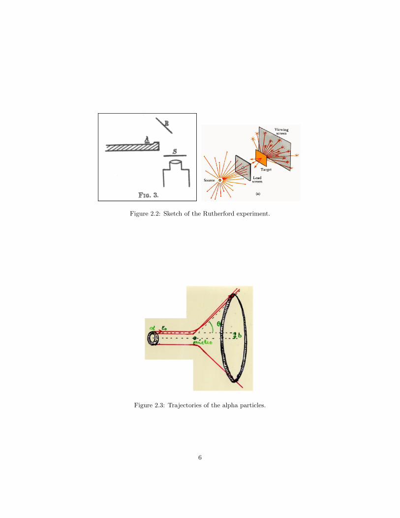
Figure 2.2: Sketch of the Rutherford experiment.

Figure 2.3: Trajectories of the alpha particles.

6

the result, using the expression for b(θ) obtained before, is:

dN

dθ= π

(1

4πε0

Q1Q2

2E0

)2 cos(θ2

)sin3

(θ2

) nbeam (2.4)

or, in terms of the solid angle Ω (dΩ = 2π sin θdθ) :

dN

dΩ=

(1

4πε0

Q1Q2

2E0

)21

sin4(θ2

) nbeam (2.5)

which is the well known Rutherford formula.

2.3 Cross-section and interaction length

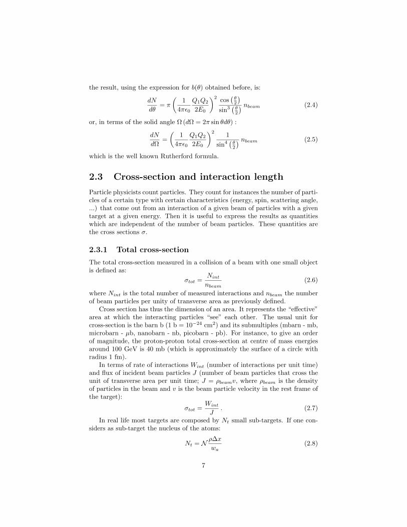
Particle physicists count particles. They count for instances the number of parti-cles of a certain type with certain characteristics (energy, spin, scattering angle,...) that come out from an interaction of a given beam of particles with a giventarget at a given energy. Then it is useful to express the results as quantitieswhich are independent of the number of beam particles. These quantities arethe cross sections σ.

2.3.1 Total cross-section

The total cross-section measured in a collision of a beam with one small objectis defined as:

σtot =Nintnbeam

(2.6)

where Nint is the total number of measured interactions and nbeam the numberof beam particles per unity of transverse area as previously defined.

Cross section has thus the dimension of an area. It represents the “effective”area at which the interacting particles “see” each other. The usual unit forcross-section is the barn b (1 b = 10−24 cm2) and its submultiples (mbarn - mb,microbarn - µb, nanobarn - nb, picobarn - pb). For instance, to give an orderof magnitude, the proton-proton total cross-section at centre of mass energiesaround 100 GeV is 40 mb (which is approximately the surface of a circle withradius 1 fm).

In terms of rate of interactions Wint (number of interactions per unit time)and flux of incident beam particles J (number of beam particles that cross theunit of transverse area per unit time; J = ρbeamv, where ρbeam is the densityof particles in the beam and v is the beam particle velocity in the rest frame ofthe target):

σtot =Wint

J. (2.7)

In real life most targets are composed by Nt small sub-targets. If one con-siders as sub-target the nucleus of the atoms:

Nt = N ρ∆x

wa(2.8)

7

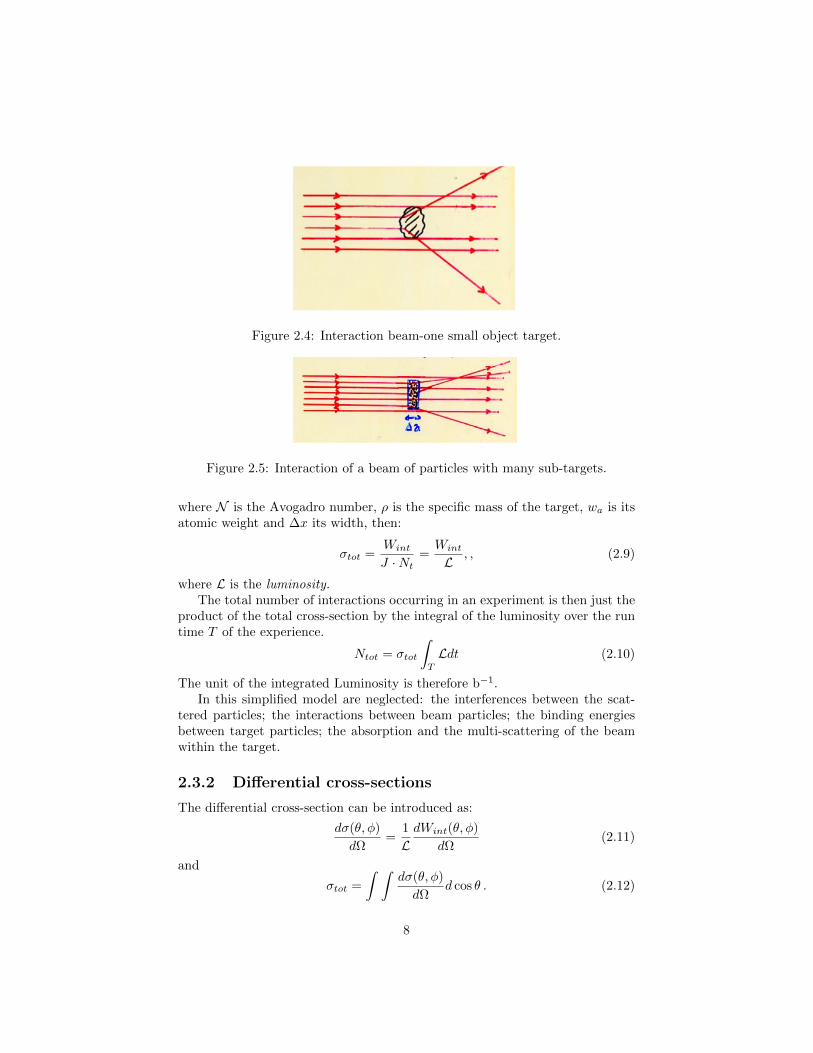
Figure 2.4: Interaction beam-one small object target.

Figure 2.5: Interaction of a beam of particles with many sub-targets.

where N is the Avogadro number, ρ is the specific mass of the target, wa is itsatomic weight and ∆x its width, then:

σtot =Wint

J ·Nt=Wint

L, , (2.9)

where L is the luminosity.The total number of interactions occurring in an experiment is then just the

product of the total cross-section by the integral of the luminosity over the runtime T of the experience.

Ntot = σtot

∫T

Ldt (2.10)

The unit of the integrated Luminosity is therefore b−1.In this simplified model are neglected: the interferences between the scat-

tered particles; the interactions between beam particles; the binding energiesbetween target particles; the absorption and the multi-scattering of the beamwithin the target.

2.3.2 Differential cross-sections

The differential cross-section can be introduced as:

dσ(θ, φ)

dΩ=

1

LdWint(θ, φ)

dΩ(2.11)

and

σtot =

∫ ∫dσ(θ, φ)

dΩd cos θ . (2.12)

8

Figure 2.6: Beam-beam interaction.

2.3.3 Cross-sections at colliders

In colliders beam/target collisions are replaced by beam/beam collisions. Par-ticles in the beams are packed in bunches. Thus the Luminosity is defined as:

L =N1N2

ATNb f (2.13)

where N1 and N2 are the number of particles in the crossing bunches, Nb is thenumber of bunches per beam, AT is the intersection transverse area and fthebeam frequency.

2.3.4 Partial cross-sections

There are often many possible results whenever two particles collide. Quantummechanics allows computing the occurring probabilities for each specific finalstate. Total cross-section is thus a sum over all possible specific final states:

σtot =∑i

σi (2.14)

where the σi are defined as the partial cross section for the specific channel i.A relevant partial cross section is the elastic cross-section σel (the particles

in the final state and in initial state are the same - there is just an exchangeof energy-momentum). Whenever there is no available energy to create newparticles, σtot = σel, as it is exemplified in Figure 2.7 in the case of the proton-proton cross-section.

2.3.5 Interaction length

The intensity of a beam is reduced whenever it crosses some piece of matter.Using the definittion of total cross-section (2.9), the reduction in a small sliceof length ∆x is:

∆N

N=Wint

J= N ρ

wA∆xσtot (2.15)

where wA is the atomic weight of the target. Defining the interaction lengthLint as:

Lint =wA

σtotNρ(2.16)

9

Figure 2.7: Proton-proton cross-section [?].

thendN

dx= − 1

LintN (2.17)

andN = N0e

−x/Lint . (2.18)

According to the above definition the unit of Lint is the unit of length (usu-ally cm). However this quantity is often redefined as

Lint =wAσtotN

(2.19)

then its unit will be g cm−2. This particular unit will be largely used in cosmicray physics. In fact the density of the atmosphere has a strong variation withheight (see next section) and thus to compute the fraction of the cosmic rayswhich have interacted along its path in the atmosphere the relevant quantity isthe amount of matter,

∫ρdx, that has been traversed.

Variation of the density of the atmosphere with height. ??

2.4 The Fermi golden rule and the Rutherfordscattering

Particles interact like “particles” but propagate like “waves”. That was theturmoil Einstein theory on the photo-electric effect introduced in Physics in

10

early XX century. In the “micro world” no more deterministic trajectories werepossible. The Newton laws had to be replaced by wave equations. Rutherfordformulae, classically deduced, are however luckily correct!

In Quantum Mechanics the scattering of a particle due to one interactionthat acts only in a finite time interval can be described as the transition betweenan initial and a final stationary states characterized by well-defined momentum.The probability λ of such transition is given, if the perturbation is small, by theFermi golden rule:

λ =2π

~|H ′fi|2ρ(Ei) (2.20)

where H ′fi is the transition amplitude between the states i and f and ρ(Ei) thedensity of final states for a given energy Ei = Ef .

The cross-section is, as it was seen above, the interaction rate per unit offlux J . Thus:

σtot =λ

J. (2.21)

Rutherford scattering can be, in first approximation, computed as a no-relativistic elastic scattering of a single particle by a fixed static Coulomb po-tential. The initial and final time independent state amplitudes may be writtenas plane waves normalized in a box of volume L3 (figure (2.8)) and with linear

momentum −→pi = ~−→ki and −→pf = ~

−→kf respectively (k=

∣∣∣−→ki ∣∣∣ =∣∣∣−→kf ∣∣∣) :

ui = L−32 exp(i

−→ki .−→r )

anduf = L−

32 exp(i

−→kf .−→r )

Assuming a scattering centre at the origin of coordinates the Coulomb potentialis written as:

V (r) =1

4πε0

Q1Q2

r

where ε0 is the vacuum dialectric constant and Q1and Q2are the charges of thebeam particle and of the target particle.

H′

fi = L−3

∫exp

(− i−→kf .−→r)V (r) exp

(− i−→ki .−→r)d3 x

introducing the momentum transfer q

−→q = ~(−→kf −

−→ki

)with

|−→q |2= 4 ~2 k2 sin2

(θ

2

)Then:

H′

fi = L−3

∫V (r) exp

(− i

~−→q .−→r

)d3 x

11

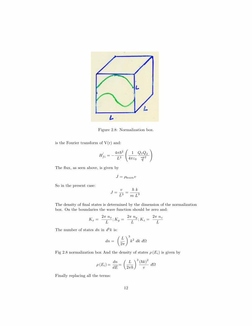
Figure 2.8: Normalization box.

is the Fourier transform of V(r) and:

H′

fi = −4π~2

L3

(1

4πε0

Q1Q2

−→q 2

)

The flux, as seen above, is given by

J = ρbeamv

So in the present case:

J =v

L3=

~ km L3

The density of final states is determined by the dimension of the normalizationbox. On the boundaries the wave function should be zero and:

Kx =2π nxL

;Ky =2π nyL

;Kz =2π nzL

The number of states dn in d3k is:

dn =

(L

2π

)3

k2 dk dΩ

Fig 2.8 normalization box And the density of states ρ (Ei) is given by

ρ (Ei) =dn

dE=

(L

2π~

)3(~k)

2

vdΩ

Finally replacing all the terms:

12

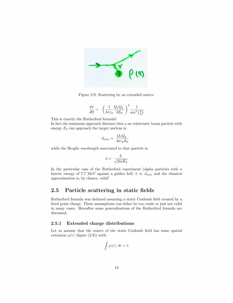
Figure 2.9: Scattering by an extended source.

dσ

dΩ=

(1

4πε0

Q1Q2

4E0

)21

sin4(θ2

)This is exactly the Rutherford formula!In fact the minimum approach distance that a no relativistic beam particle withenergy E0 can approach the target nucleus is:

dmin =Q1Q2

4πε0E0

while the Broglie wavelength associated to that particle is:

λ =h√

2mE0

In the particular case of the Rutherford experiment (alpha particles with akinetic energy of 7.7 MeV against a golden foil) λ dmin and the classicalapproximation is, by chance, valid!

2.5 Particle scattering in static fields

Rutherford formula was deduced assuming a static Coulomb field created by afixed point charge. These assumptions can either be too crude or just not validin many cases. Hereafter some generalizations of the Rutherford formula arediscussed.

2.5.1 Extended charge distributions

Let us assume that the source of the static Coulomb field has some spatialextension ρ(r) (figure (2.9)) with:∫

ρ (r) dr = 1

13

Then

H′

fi = L−3

∫ (1

4πε0

Q1Q2 ρ (r)

r

)exp

(− i

~−→q .−→r

)d3 x

and defining the electric form factor F (q) as

F (q) =

∫ρ (r) exp

(− i

~−→q .−→r

)d3 x

the modified scattering cross-section is

dσ

dΩ= |F (−→q )|2

(dσ

dΩ

)0

where(dσdΩ

)0

is the Rutherford cross-section.In the case of the proton ρ (r) ∝ exp (− b r) , with b ' 0.71 GeV/c and so(diple formula):

F (q) ∝

(1 +−→q 2

b2

)−2

2.5.2 Finite range interactions

Coulomb field, as the Newton gravitational field, has an infinite range. Letus now assume that there is an exponential attenuation on the field (Yukawapotential):

V (r) =g

4πrexp(− r

a)

where a is some range scale.Then

H′

fi = L−3

∫ ( g

4πrexp(− r

a))

exp

(− i

~−→q .−→r

)d3 x

H′

fi = − ~2

L3

(g

−→q 2+ 1

a2

)and

dσ

dΩ= g2ε2

0

( −→q 2

−→q 2+M2c2

)2 (dσ

dΩ

)0

where(dσdΩ

)0

is the Rutherford cross-section. M = 1/ac can be interpreted, asit will be discussed later on, as the mass of an exchange particle (a = 1 fmcorresponds to M ' 200 MeV/c).

14

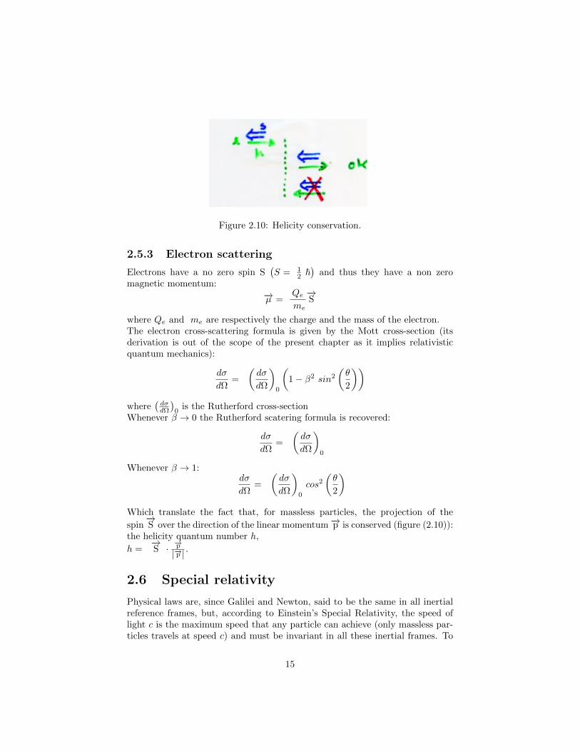
Figure 2.10: Helicity conservation.

2.5.3 Electron scattering

Electrons have a no zero spin S(S = 1

2 ~)

and thus they have a non zeromagnetic momentum:

−→µ =Qeme

−→S

where Qe and me are respectively the charge and the mass of the electron.The electron cross-scattering formula is given by the Mott cross-section (itsderivation is out of the scope of the present chapter as it implies relativisticquantum mechanics):

dσ

dΩ=

(dσ

dΩ

)0

(1− β2 sin2

(θ

2

))where

(dσdΩ

)0

is the Rutherford cross-sectionWhenever β → 0 the Rutherford scatering formula is recovered:

dσ

dΩ=

(dσ

dΩ

)0

Whenever β → 1:dσ

dΩ=

(dσ

dΩ

)0

cos2

(θ

2

)Which translate the fact that, for massless particles, the projection of the

spin−→S over the direction of the linear momentum −→p is conserved (figure (2.10)):

the helicity quantum number h,

h =−→S ·

−→p|−→p | .

2.6 Special relativity

Physical laws are, since Galilei and Newton, said to be the same in all inertialreference frames, but, according to Einstein’s Special Relativity, the speed oflight c is the maximum speed that any particle can achieve (only massless par-ticles travels at speed c) and must be invariant in all these inertial frames. To

15

Figure 2.11: Inertial reference frames.

cope with these two postulates a deep change in our perception of space andtime was needed: time and length are no longer absolute; two simultaneousevents in one reference frame are not simultaneous in any other reference framethat moves with a nonzero velocity in relation to the first one; Galilei trans-formation have to be replaced by new ones (Lorentz transformations); mass isjust a particular form of energy; kinematics at velocities near c is quite differentfrom the usual one and particle physics is the laboratory to test it.

2.6.1 Lorentz transformations

Let S and S’ be two inertial reference frames that move one in relation to theother, at a constant velocity ~v directed along the x axis (Figure 2.11). Thenthe coordinates in one reference frame transform into new coordinates (Lorentztransformation) as:

ct = γ(ct′ + β x′)

x = γ(x′ + β ct′)

y = y′

z = z′

where β = v/c and γ = 1/√

1− β2.For an observer in S the time interval measured by a clock in S’ is larger

(time dilatation):∆T = γ∆T ′

while the length of a ruler that is at rest in S’ is shorter (length contraction):

∆L = γ∆L′/γ .

16

Defining time-position four vectors xµ (µ = 0, 1, 2, 3) as:

x0 = ct ; x1 = x ; x2 = y ; x3 = z

the Lorentz transformations can be written in a matricial way: with

xµ = Λµνxν

with

Λµν =

γ γβ 0 0γβ γ 0 00 0 1 00 0 0 1

.

2.6.2 Space-time interval

Time and space intervals are no longer invariants. However a combination ofboth is a Lorentz invariant. Defining the space-time interval ∆s and ∆s′ as:

∆s2 = (c∆t)2 − (∆x2 + ∆y2 + ∆z2)

∆s′2 = (c∆t′2)2 − (∆x′2 + ∆y′2 + ∆z′2)

then, using the Lorentz transformation it can be shown that:

∆s2 = ∆s′2 .

Two events can be:

∆s2 > 0 (“time− like” interval)

∆s2 = 0

∆s2 < 0 (“space− like” interval) .

The space-time is divided thus into two regions by the cone of the ∆s2 = 0events (the so-called light cone). The interval between two causal events isalways “time-like” (no time travels, sorry).

∆s2 can be obtained as a scalar product of xµ with itself:

∆s2 = xµxµ

or∆s2 = gµνx

µxν

being gµν the Minkowski metric matrix:

gµν =

1 0 0 00 −1 0 00 0 −1 00 0 0 −1

.

17

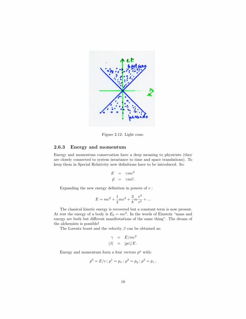
Figure 2.12: Light cone.

2.6.3 Energy and momentum

Energy and momentum conservation have a deep meaning to physicists (theyare closely connected to system invariance to time and space translations). Tokeep them in Special Relativity new definitions have to be introduced. So:

E = γmc2

~p = γm~v .

Expanding the new energy definition in powers of v :

E = mc2 +1

2mv2 +

3

8mv4

c2+ ...

The classical kinetic energy is recovered but a constant term is now present.At rest the energy of a body is E0 = mc2. In the words of Einstein “mass andenergy are both but different manifestations of the same thing”. The dream ofthe alchemists is possible!

The Lorentz boost and the velocity β can be obtained as:

γ = E/mc2

|β| = |pc|/E .

Energy and momentum form a four vectors pµ with:

p0 = E/c ; p1 = px ; p2 = py ; p3 = pz ,

18

Figure 2.13: Two-to-two particle scattering.

and the same Lorentz transformations, valid for any four-vector, apply:

E/c = γ(E′/c+ β p′x)

px = γ(p′x + β E′/c)

py = p′y

pz = p′z

The scalar product of pµ with itself is by definition invariant and gives:

p2 = pµpµ = (E/c)2 − |~p|2 = m2c4

and thusE2 = m2c4 + |~p|2c2 .

For massless particles (as the photon):

E = pc .

2.6.4 Mandelstam variables

The kinematics of two to two particle scattering can be expressed in terms ofLorentz invariant scalars, the Mandelstam variables s, t, u, obtained as thesquare of the sum (or subtraction) of two of the intervenient particles four-vectors.

If p1 and p2 are the four-vectors of the incoming particles and p3 and p4 arethe four-vectors of the outgoing particles, the Mandelstam variables are definedas:

s = (p1 + p2)2

t = (p1 − p3)2

u = (p1 − p4)2 .

The s variable is the square of the centre-of-mass energy. In the centre-of-mass reference frame S∗ :

s =((E∗1 , ~p

∗) + (E∗1 ,− ~p∗))2

= E2CM = (E∗1 + E∗2 )2

19

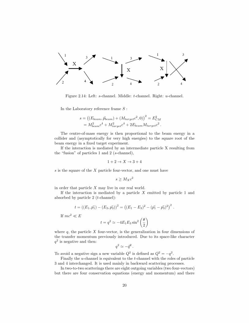
Figure 2.14: Left: s-channel. Middle: t-channel. Right: u-channel.

In the Laboratory reference frame S :

s =((Ebeam, ~pbeam) + (Mtargetc

2, 0))2

= E2CM

= M2beamc

4 +M2targetc

4 + 2EbeamMtargetc2 .

The centre-of-mass energy is then proportional to the beam energy in acollider and (asymptotically for very high energies) to the square root of thebeam energy in a fixed target experiment.

If the interaction is mediated by an intermediate particle X resulting fromthe “fusion” of particles 1 and 2 (s-channel),

1 + 2→ X → 3 + 4

s is the square of the X particle four-vector, and one must have

s ≥MXc2

in order that particle X may live in our real world.If the interaction is mediated by a particle X emitted by particle 1 and

absorbed by particle 2 (t-channel):

t = ((E1, ~p1)− (E3, ~p3))2

=((E1 − E3)2 − (~p1 − ~p3)2

)2.

If mc2 E

t = q2 ' −4E1E3 sin2

(θ

2

)where q, the particle X four-vector, is the generalization in four dimensions ofthe transfer momentum previously introduced. Due to its space-like characterq2 is negative and then:

q2 ' −~q2 .

To avoid a negative sign a new variable Q2 is defined as Q2 = −q2.Finally the u-channel is equivalent to the t-channel with the roles of particle

3 and 4 interchanged. It is used mainly in backward scattering processes.In two-to-two scatterings there are eight outgoing variables (two four-vectors)

but there are four conservation equations (energy and momentum) and there

20

are relations between the energy of each outgoing particle and its momentum(see previous section). Then there are only two independent outgoing variablesand s, t, u must be related. In fact:

s+ t+ u = m1c2 +m2c

2 +m3c2 +m4c

2 .

2.6.5 Lorentz invariant transition rates, phase space, fluxesand cross-sections

In not relativistic Quantum Mechanics probability density |ψ(~r)|2 is usuallynormalized to 1 in some arbitrary box of volume V. However, V is not a Lorentzinvariant and therefore the transition amplitude H ′fi, the density of final statesρ(Ei) and the flux J as defined previously are not Lorentz invariant! Theadopted convention is to normalize the density of probability to 2E (EV is aLorentz invariant and the factor 2 is historical). Then the transition rate isredefined as:

λ =2π

~|M|2∏ni

i=1 2Eiρnf

(E)

where the scattering amplitude is

|M|2 = |H ′fi|2ni∏i=1

2Ei

nf∏f=1

2Ef

and the relativistic phase space is

ρnf(E) =

1

2π~)3nf

∫ nf∏f=1

2Efδ

nf∑f=1

~pf − ~p0

δ

nf∑f=1

Ef − E0

.

ni and nf are the number of particles in the intial and final states respectivelyand the δ functions ensures the conservation of linear momentum and energy.

In the case of a two body final state the phase space in the centre of massframe is just:

ρ2(E∗) =π

(2π~)6

| ~p∗|E∗

where ~p∗ and E∗ are respectively the linear momentum of each final state particleand the total energy in the centre of mass reference frame.

The flux is now defined as :

J = 2Ea2Ebvab = 4F

where vab is the relative velocity of the two interacting particles and F theMller’s invariant flux factor.In term of the four-vectors and pa and pb of the incoming particles:

F =

√(pa.pb )

2 −ma2mb

2c4

21

or in terms of invariant variables

F =

√(s− (mac2 +mbc2)

2)(

s− (mac2 −mbc2)2)

Putting together all the factors the cross section of two interacting particles isgiven by:

σa+b→1+2+···+nf=

1

4F

S~2

(2π)3nf−4

∫|M|2

nf∏f=1

d3pf2Ef

δ

nf∑f=1

−→pf −−→p0

δ nf∑f=1

Ef − E0

Where S is a statistical factor that correct for double counting whenever thereare identical particles and accounts also for spin statistics.In the special case of a two to two body scattering in the centre of mass framea simple expression for the differential cross section dσ

dΩ can thus be obtained (

if |M|2 is a function of final momentum the angular integration can not becarried out):

dσ

dΩ=

(~c8π

)2S |M|2

s

|−→pf ||−→pi |

2.7 Decays

Stable particles like the proton, the electron and the photon (as much as weknow) are the exception, not the rule. The lifetime of most particles is finiteand its value may span over many orders of magnitude from, for instance, 10−25

s for the electroweak massive bosons (Z and W ) to around 900 s for the neutron,depending on the strength of the relevant interaction and on the size of the decayphase space.

Stable particles are described by pure harmonic wave functions and theirFourier transforms are just functions centred in well defined proper energiesE = mc2 (figure (2.15)):

Ψ(t) ∝ Ψ(0)e−iE~ t

Ψ(E) ∝ δ(E −mc2) .

Unstable particles are described by damped harmonic wave functions andtherefore their proper energies are not well defined (figure (2.16)):

Ψ(t) ∝ Ψ(0)e−iE~ te−i

Γ2~ t =⇒ |Ψ(t)|2 ∝ |Ψ(0)|2e−t/τ

Ψ(E) ∝ 1

(E −mc2) + iΓ/2=⇒ |Ψ(E)|2 ∝ 1

(E −mc2)2 + Γ2/4

which is a Cauchy function (physicists usually call it a Breit-Wigner function)for which the witht Γ is thus directly related to the particle lifetime τ :

τ =~Γ.

22

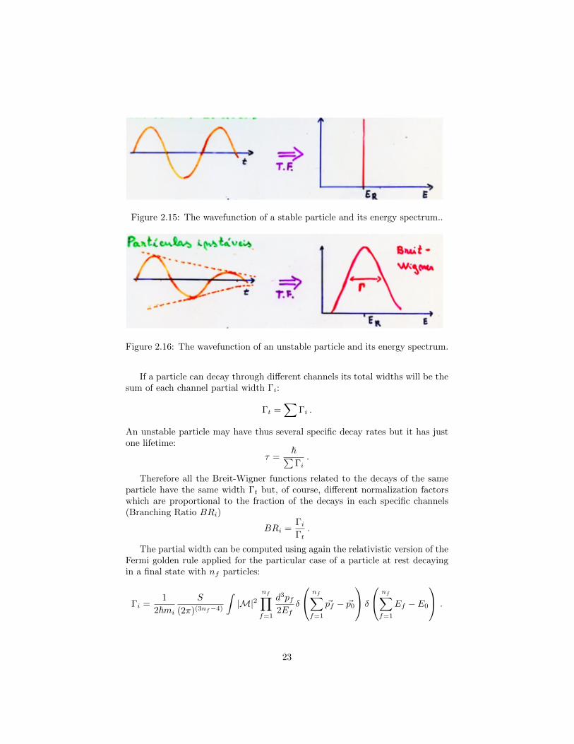
Figure 2.15: The wavefunction of a stable particle and its energy spectrum..

Figure 2.16: The wavefunction of an unstable particle and its energy spectrum.

If a particle can decay through different channels its total widths will be thesum of each channel partial width Γi:

Γt =∑

Γi .

An unstable particle may have thus several specific decay rates but it has justone lifetime:

τ =~∑Γi.

Therefore all the Breit-Wigner functions related to the decays of the sameparticle have the same width Γt but, of course, different normalization factorswhich are proportional to the fraction of the decays in each specific channels(Branching Ratio BRi)

BRi =ΓiΓt.

The partial width can be computed using again the relativistic version of theFermi golden rule applied for the particular case of a particle at rest decayingin a final state with nf particles:

Γi =1

2~mi

S

(2π)(3nf−4)

∫|M|2

nf∏f=1

d3pf2Ef

δ

nf∑f=1

~pf − ~p0

δ

nf∑f=1

Ef − E0

.

23

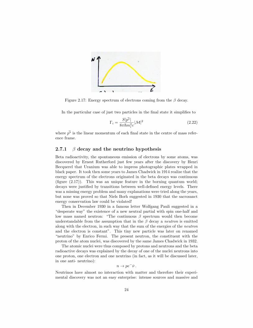
Figure 2.17: Energy spectrum of electrons coming from the β decay.

In the particular case of just two particles in the final state it simplifies to

Γi =S| ~p∗|

8π~m2i c|M|2 (2.22)

where ~p∗ is the linear momentum of each final state in the centre of mass refer-ence frame.

2.7.1 β decay and the neutrino hypothesis

Beta radioactivity, the spontaneous emission of electrons by some atoms, wasdiscovered by Ernest Rutherford just few years after the discovery by HenriBecquerel that Uranium was able to impress photographic plates wrapped inblack paper. It took then some years to James Chadwick in 1914 realize that theenergy spectrum of the electrons originated in the beta decays was continuous(figure (2.17)). This was an unique feature in the borning quantum world;decays were justified by transitions between well-defined energy levels. Therewas a missing energy problem and many explanations were tried along the years,but none was proved so that Niels Borh suggested in 1930 that the sacrosanctenergy conservation law could be violated!

Then in December 1930 in a famous letter Wolfgang Pauli suggested in a“desperate way” the existence of a new neutral partial with spin one-half andlow mass named neutron: “The continuous β spectrum would then becomeunderstandable from the assumption that in the β decay a neutron is emittedalong with the electron, in such way that the sum of the energies of the neutronand the electron is constant”. This tiny new particle was later on renamed“neutrino” by Enrico Fermi. The present neutron, the constituent with theproton of the atom nuclei, was discovered by the same James Chadwick in 1932.

The atomic nuclei were thus composed by protons and neutrons and the betaradioactive decays was explained by the decay of one of the nuclei neutrons intoone proton, one electron and one neutrino (in fact, as it will be discussed later,in one anti- neutrino):

n→ pe−ν .

Neutrinos have almost no interaction with matter and therefore their experi-mental discovery was not an easy enterprise: intense sources and massive and

24

performant detectors had to be made. Only in 1956 Reines and Cowen provedthe neutrino existence placing an instrumented water tank near a nuclear reac-tor. Some of the anti-neutrino produced in the reactor interacted in the waterwith one proton giving raise to one neutron and a positron (the anti-particle ofthe electron), the so called inverse beta decay:

νp→ ne+ .

The positron would then annihilate with an ordinay electron and the neutronmay be captured by some cadmium chloride atoms dissolved in the water. Threephotons were then detected (two from the annihilation and 5 microseconds lateranother from the excited cadmium atom).

The mass of the neutrino is indeed very low (but not zero, as discovered atthe end of the XX century with the observation of neutrino oscillations) anddetermines the maximum energy that the electron may have in the beta decay(the energy spectrum end point). The present measurements are compatiblewith neutrino masses bellow a few eV.

2.8 Fields and particles

Particle interactions are described by fields. Fields were, in classical mechanics,just a mathematical abstraction; the real thing were the forces. The paradig-matic example was the instantaneous and universal Newton’s gravitation law.Later on, Maxwell gave to the electromagnetic field the status of a physics en-tity: it transports energy and momentum in the form of electromagnetic wavesand propagates at a finite velocity - the speed of light. Then, Einstein explainedthe photo-electric effect postulating the existance of photons - the interaction ofthe electromagnetic waves with free electrons, as discovered by Compton, wasequivalent to elastic collisions between two particles: the photon and the elec-tron. Finally with Quantum Mechanics the wave-particle duality was extendedto all field and matter particles.

Field particles and matter particles have however striking different behaviours.While there is no limit for the number of identical and indistinguishable field par-ticles that can be in the same quantum state (field particles obey Bose-Einsteinstatistics and are called bosons), the matter particles are under the rule of thePauli exclusion principle - only one single particle can occupy a given quantumstate (matter particles obey Fermi-Dirac statistics and are called fermions).Lasers (coherent streams of photons) and the electronic structure of atoms arejustified.

The spin of the particle and the statistics it obeys are connected by the spin-statistic theorem. According to this highly non trivial theorem, demonstratedby Fierz and Pauli in 1939 and 1940 respectively, fermions have half-integerspins while bosons have integer spins.

Behind the gravitational and the electromagnetic interactions there was theneed to introduce in the XX century two new fundamental interactions: thestrong and the weak interactions. The strong interaction ensures for instance

25

the stability of atomic nuclei and the weak interaction the beta decay and thusthe energy production at the Sun. The boson associated to gravitation is thegraviton (not yet experimentally discovered), to electromagnetism the photon,to strong interaction the gluons (there are eight!) and to weak interaction themassive bosons W±, and the neutral Z.

The couplings of each particle to the boson(s) associated to a given interac-tion are determined by magic numbers called charges. The gravitational chargeis, in Einstein’s general relativity version, its energy-momentum tensor, theelectrical charges are the well-known positive and negative charges, the strongcharges are three and designated by colours names (red, green, blue), and theweak charges are the weak isospin charges (±1/2 for fermions, 0, ±1 for bosons).

The relative intensity of such interactions spans many orders of magnitude.In a scale where the intensity of strong interactions is 1: the intensity electro-magnetic interactions is 10−2; the intensity of weak interactions is 10−13 andfinally the intensity of gravitational interactions is 10−38. Contrary to the grav-itational interaction, particles or combination of particles can be neutral to theother interactions. For instances electrons have electric and weak charges butno colour charge, and atoms are electrically neutral. At astrophysical scales thedominant interaction is gravitation, at the object scale is the electromagneticinteraction, at the scale of nuclei is the strong one.

Quantum vacuum is not empty at all. Heisenberg’s incertitude relationsallow energy violations by a quantity ∆E within small time intervals ∆t suchthat ∆t ∼ ~/∆E. Massive particles that “live” in such tiny time intervals arecalled “virtual”. But besides such particles which are in the origin of measurableeffects (like the Casimir effect) we have just discovered that space is filled, as itwould be discussed below, by an extra field: the Higgs field (a boson of spin 0).Particles in the present theory are intrinsically massless. It is their interactionwith the Higgs field that originate some kind of effective mass: a new Ethercould be conjectured.

2.9 Units

The International system of units (SI) can be constructed on the basis of fourfundamental units: of length (the meter m), of time (the second s), of mass (thekilogram kg), of charge (the coulomb C)1.

These units are inappropriate for the world of fundamental physics: theradius of a nucleus is of the order of 10−15 m, also called one femtometer (fm)or one fermi; the mass me of an electron is of the order of 10−30 kg; the chargeof an electron is (in absolute value) of the order of 10−19 C. By using such unitswe would carry along a lot of exponents! Thus in particle physics we better useunits like the electron charge for the electrostatic charge, and the electronvolteV and its multiples (keV, MeV, GeV, TeV) for the energy.

1For reasons related only to metrology, i.e., of reproducibility and accuracy of the definition,in the standard SI the unit of electrical current, the ampere A, is used instead of the coulomb;the two definitions are however conceptually equivalent.

26

Length 1 fm 10−15 mMass 1 MeV/c2 1.78× 10−30 kgCharge |e| 1.60× 10−19 C

Note the unit of mass, in which the relation E = mc2 is used implicitly:what one is doing here is to use 1 eV ' 1.60× 10−19 J as the new fundamentalunit of energy.

With these new units, the mass of a proton is about 0.938 GeV/c2, and themass of the electron is about 0.511 MeV/c2. The fundamental energy level ofHydrogen is about −13.6 eV.

In addition to this, nature is providing us with two constants which areparticularly appropriate for the world of fundamental physics: the speed of lightc ' 3.00×108 m/s = 3.00×1023 fm/s, and the Planck’s constant ~ ' 1.05×10−34

J s ' 6.58× 10−16 eV s.It seems then natural to express speeds in terms of c, and angular moments

in terms of ~. When we do this we switch to the so-called Natural Units (NU).The minimal set of natural units (not including electromagnetism) could thenbe

Speed 1 c 3.00× 108 m/sAngular momentum 1 ~ 1.05× 1034 J sEnergy 1 eV 1.60× 10−19 J

In such a system, ~ = c = 1.After these conventions, just one unit can be used to describe the mechanical

Universe: we choose energy, and thus we can express al mechanical quantitiesin terms of eV and of its multiples. It is immediate to express momenta andmasses directly in NU. To express 1 m and 1 s , we can just write 2

1m = 1m~c ' 5.10× 1012MeV−1

1s = 1s~ ' 1.52× 1021 .MeV−1

Both length and time are thus, in natural units, expressed as inverse ofenergy.

The first relation can also be written as 1fm ' 5.10GeV−1: note that whenyou have a quantity expressed in MeV−1, in order to express it in GeV−1, youmust multiply (and not divide) by a factor of 1000.

Let us now find a general rule to transform quantities expressed in naturalunits into SI units, and vice-versa.

To express a quantity in NU back to SI we first restore the ~ and c factorsby dimensional arguments and then use the conversion factors ~ and c (or ~c)to evaluate the result. The dimension of c is [c] = [m/s]; the dimension of ~ is[kgm2s−1].

2~c ' 1.97× 10−13MeV m = 3.15× 10−26J m

27

mks NUQuantity p q r nMass 1 0 0 0Length 0 1 0 -1Time 0 0 1 -1Action (~) 1 2 -1 0Velocity (c) 0 1 -1 0Momentum 1 1 -1 1Energy 1 2 -2 1

Table 2.1: Dimensions of different physical quantities in the SI and NU.

The vice-versa (from SI to NU) is also easy. A quantity with metre-kilogram-second (mks) dimensions MpLqT r (where M represents the mass, L the lengthand T the time) has the NU dimensions [Ep−q−r], where E represents energy.Since ~ and c do not appear in NU, this is the only relevant dimension, anddimensional checks and estimates are very simple. The quantity Q in the SI canbe expressed in NU as

QNU = QSI

(5.62× 1029 MeV

kg

)p(5.10× 1012 MeV−1

m

)q×

(1.52× 1021 MeV−1

s

)rMeVp−q−r

The NU and SI dimensions are listed for some important quantities in Table2.1.

Note that by choosing natural units, all factors of ~ and c may be omittedfrom equations, which leads to considerable simplifications (and, in the nextchapters, we will profit from it!). For example, the relativistic energy relation

E2 = p2c2 +m2c4

becomesE2 = p2 +m2

Finally, let us discuss how to treat electromagnetism. To do so, we mustintroduce a new unit, charge for example. We can redefine the unit charge byobserving that

e2

4πε0

has the dimension of [J m], and thus is a pure number in NU. By dividing by~c one has:

e2

4πε0~c' 1

137.

Imposing that the electric permeability of vacuum ε0 = 1 (thus automaticallyµ0 = 1 for the magnetic permeability of vacuum, since from Maxwell’s equations

28

ε0µ0 = 1/c2) we obtain the new definition of charge, and with such a definition:

α =e2

4π' 1

137.

This is called the Lorentz-Heaviside convention. Elementary charge in NU be-comes then a pure number:

e ' 0.303 .

Let use make some applications.

The Thomson cross section. Let us express in NU a cross section. The crosssection for Compton scattering of a photon by a free electron is for E mec

2

(Thomson regime)

σT '8πα2

3m2e

. (2.23)

The dimension of a cross section must be, in SI, [m2]. Thus we can write

σT '8πα2

3m2e

~acb (2.24)

and determine a and b such that the result has the dimension of a length squared.We find a=2 and b=-2; thus

σT '8πα2

3(mec2)2(~c)2 (2.25)

and thus σT ' 6.65× 1029 m2 = 665 mb.

The Planck mass, length, time. Quantum theory says that associated toany mass m there is a length called the Compton wavelength, λC , which isdefined as the wavelength of a photon with an energy equal to the rest mass ofthe particle.

λC =h

mc= 2π

~mc

.

Thus the Compton wavelength sets the distance scale at which quantum fieldtheory becomes crucial for understanding the behavior of a particle of a givenmass.

On the other hand, general relativity says that associated to any mass mthere is a Schwarzschild radius, RS , such that compressing an object of mass mto a size smaller than this radius results in the formation of a black hole. TheSchwarzschild radius gives the distance scale at which general relativity becomescrucial for understanding the behavior of an object of a given mass. We have

RS =2GNm

c2

where GN is the gravitational constant.

29

We call the Planck mass the mass at which the Schwarzschild radius of a par-ticle becomes equal to its Compton length, and the Planck length their commonvalue when this happens. The probe who could locate a particle within this dis-tance would collapse to a black hole, something that would make measurementsvery weird. In NU, one can write

2π

mP= 2GNmP → mP =

√π

GN

which can be converted into

mP =

√π~cGN' 3.86× 10−8kg ' 2.16× 1019GeV/c2 .

Since we are talking about orders of magnitude, the factor√π is often ne-

glected and we take as a definition:

mP =

√~cGN' 2.18× 10−8kg ' 1.22× 1019GeV/c2 .

Besides the Planck length `P , we can also define a Planck time tP = `P /c(their value is equal in NU):

`P = tP =1

mP=√GN

(this corresponds to a length of about 1.6 × 10−20 fm, and to a time of about5.4× 10−44 s).

We expect that both general relativity and quantum field theory would beneeded to understand the behavior of an object whose mass is about the Planckmass and whose radius is about the Planck length, or when we talk about timescomparable to the Planck time. Traditional quantum physics and gravitationcertainly fall short at this scale; since this failure should be independent ofthe reference frame, many scientists think that the Plank scale should be aninvariant irrespective of the reference frame in which it is calculated (this factwould of course require important modifications to the theory of relativity).

Note that the shortest length you can probe with the energy of a particle ac-celerated by LHC (which is expected to be of 7 TeV in the future, correspondingto the collision of a proton of about 105 TeV with a proton at rest) is about 1011

times larger than the Planck length scale. Cosmic protons can reach an energyof 1021 eV, i.e., a distance about 107 times larger than the Planck length scale.Indirect measurements with cosmic rays allow testing effects very close to thePlanck scale. Cosmic rays are at the frontier of the exploration of fundamentalscales.

30