lable at ScienceDirect

Quaternary Science Reviews 29 (2010) 113–128

Contents lists avai

Quaternary Science Reviews

journal homepage: www.elsevier .com/locate/quascirev

EPICA Dome C record of glacial and interglacial intensities

V. Masson-Delmotte a,*, B. Stenni b, K. Pol a, P. Braconnot a, O. Cattani a, S. Falourd a, M. Kageyama a,J. Jouzel a, A. Landais a, B. Minster a, J.M. Barnola c, J. Chappellaz c, G. Krinner c, S. Johnsen d,R. Rothlisberger e, J. Hansen f,g, U. Mikolajewicz h, B. Otto-Bliesner i

a Laboratoire des Sciences du Climat et de l’Environnement, IPSL, UMR CEA CNRS UVSQ 1572, CEA Saclay, Bat. 701, L’Orme des Merisiers, 91 191 Gif-sur-Yvette cedex, Franceb Universita di Trieste, Dipartimento di Scienze Geologiche, Ambientali e Marine, Via E. Weiss 2, 34127 Trieste, Italyc Laboratoire de Glaciologie et Geophysique de l’Environnement, UMR CNRS UJF 5183, 54 rue Moliere, 38 402 Saint Martin d’Heres cedex, Franced Geophysical Department, Juliane Maries Vej 30, DK-2100 Kobenhavn, Denmarke British Antarctic Survey, High Cross, Madingley Road, Cambridge CB3 0ET, United Kingdomf NASA/Goddard Institute for Space Studies, New York, NY 10025, USAg Columbia University Earth Institute, New York, NY 10027, USAh Max-Planck-Institute for Meteorology, Bundesstrasse 53, D-20146 Hamburg, Germanyi CCR, CGD/NCAR, PO Box 3000, Boulder, CO 80307-3000, USA

a r t i c l e i n f o

Article history:Received 19 December 2008Received in revised form29 September 2009Accepted 30 September 2009

* Corresponding author. Tel.: þ33 1 69 08 77 15; faE-mail address: valerie.masson@cea.fr (V. Masson

0277-3791/$ – see front matter � 2009 Elsevier Ltd.doi:10.1016/j.quascirev.2009.09.030

a b s t r a c t

Climate models show strong links between Antarctic and global temperature both in future and in glacialclimate simulations. Past Antarctic temperatures can be estimated from measurements of water stableisotopes along the EPICA Dome C ice core over the past 800 000 years. Here we focus on the reliability ofthe relative intensities of glacial and interglacial periods derived from the stable isotope profile. Theconsistency between stable isotope-derived temperature and other environmental and climatic proxiesmeasured along the EDC ice core is analysed at the orbital scale and compared with estimates of globalice volume. MIS 2, 12 and 16 appear as the strongest glacial maxima, while MIS 5.5 and 11 appear as thewarmest interglacial maxima.

The links between EDC temperature, global temperature, local and global radiative forcings areanalysed. We show: (i) a strong but changing link between EDC temperature and greenhouse gas globalradiative forcing in the first and second part of the record; (ii) a large residual signature of obliquity inEDC temperature with a 5 ky lag; (iii) the exceptional character of temperature variations withininterglacial periods.

Focusing on MIS 5.5, the warmest interglacial of EDC record, we show that orbitally forced coupledclimate models only simulate a precession-induced shift of the Antarctic seasonal cycle of temperature.While they do capture annually persistent Greenland warmth, models fail to capture the warmingindicated by Antarctic ice core dD. We suggest that the model-data mismatch may result from the lack offeedbacks between ice sheets and climate including both local Antarctic effects due to changes in icesheet topography and global effects due to meltwater–thermohaline circulation interplays. An MIS 5.5sensitivity study conducted with interactive Greenland melt indeed induces a slight Antarctic warming.We suggest that interglacial EDC optima are caused by transient heat transport redistribution compa-rable with glacial north–south seesaw abrupt climatic changes.

� 2009 Elsevier Ltd. All rights reserved.

1. Introduction

Glacial–interglacial climate change is expected to result fromthe orbital forcing, changes in atmospheric composition andinternal feedbacks, such as changes in planetary albedo (Paillard,

x: þ33 1 69 08 77 16.-Delmotte).

All rights reserved.

1998). Along the last million years, changes in land–seageographical distribution can be considered as negligible in drivingpast changes in climate and atmospheric composition, in contrastwith deeper times. Over this time period, the orbital forcing is wellknown from astronomical calculations (Berger and Loutre, 1991;Laskar et al., 1993). It is therefore critical to document the relativeintensities of past glacial and interglacial periods, in terms ofchanges in atmospheric composition and global temperatures. Eachclimate archive provides a complementary view of the global

V. Masson-Delmotte et al. / Quaternary Science Reviews 29 (2010) 113–128114

climate system. Globally relevant climate data can be extractedfrom marine records, where proxies document past changes intropical sea surface temperature (Lea, 2004), deep ocean temper-ature (Zachos et al., 2001), or past changes in sea level (Bintanjaet al., 2005; Lisiecki and Raymo, 2005), or from continental recordsdocumenting past changes in vegetation cover (Cheddadi et al.,2005; Tzedakis et al., 2006) or monsoon intensity (Sun et al., 2006;Wang et al., 2008).

There are specific areas, such as the tropics or Antarctica (Fig. 1),where climate models show a strong link between local tempera-ture changes and global temperature changes (Lea, 2004; Masson-Delmotte et al., 2006a; Schneider von Deimling et al., 2006;Hargreaves et al., 2007; IPCC, 2007). Here, we focus on deepAntarctic ice cores. They offer a variety of new climate and envi-ronmental records including the documentation of past atmo-spheric composition over several glacial–interglacial cycles, atVostok (Petit et al., 1999), Dome Fuji (Watanabe et al., 2003;Kawamura et al., 2007) or EPICA Dome C (Jouzel et al., 2007;Loulergue et al., 2008; Luthi et al., 2008). Recently, multipleparameters have been measured on the EPICA Dome C (hereafterEDC) ice core spanning the past 800 000 years (Section 2).

These parameters track climate changes from a variety of lati-tudes. Past temperatures are relevant for central Antarctica. Pastchanges in sea salt sodium have been suggested to be related to seaice surface area, modulated by uplift and transport from the sea icesurface towards central Antarctica. Past changes in methaneconcentrations are relevant for continental wetland temperatureand moisture, mainly in the tropics and the Northern Hemisphere.Past changes in carbon dioxide concentration are relevant forchanges in terrestrial and marine carbon sources and sinks, andpast changes in dust or non-sea-salt calcium are expected todocument dust production on southern hemisphere mid-latitudecontinents and its transport to Antarctica. Recent studies havebeen conducted on the sequence of events during terminations(Rothlisberger et al., 2008), but this approach remains difficult toextend to the phase relationships between atmospheric composi-tion and climate due to relative dating uncertainties for the gas andthe ice records caused by firnification processes (Caillon et al.,2003; Loulergue et al., 2007).

Section 3 is focused on the relative intensity of glacial andinterglacial extrema as identified in various ice core proxies. First,we discuss the uncertainties on past Antarctic temperatures which

-10

-8

-6

-4

-2

0

2

4)C°( egnahc erutarep

meT

4002000

Age (ka B

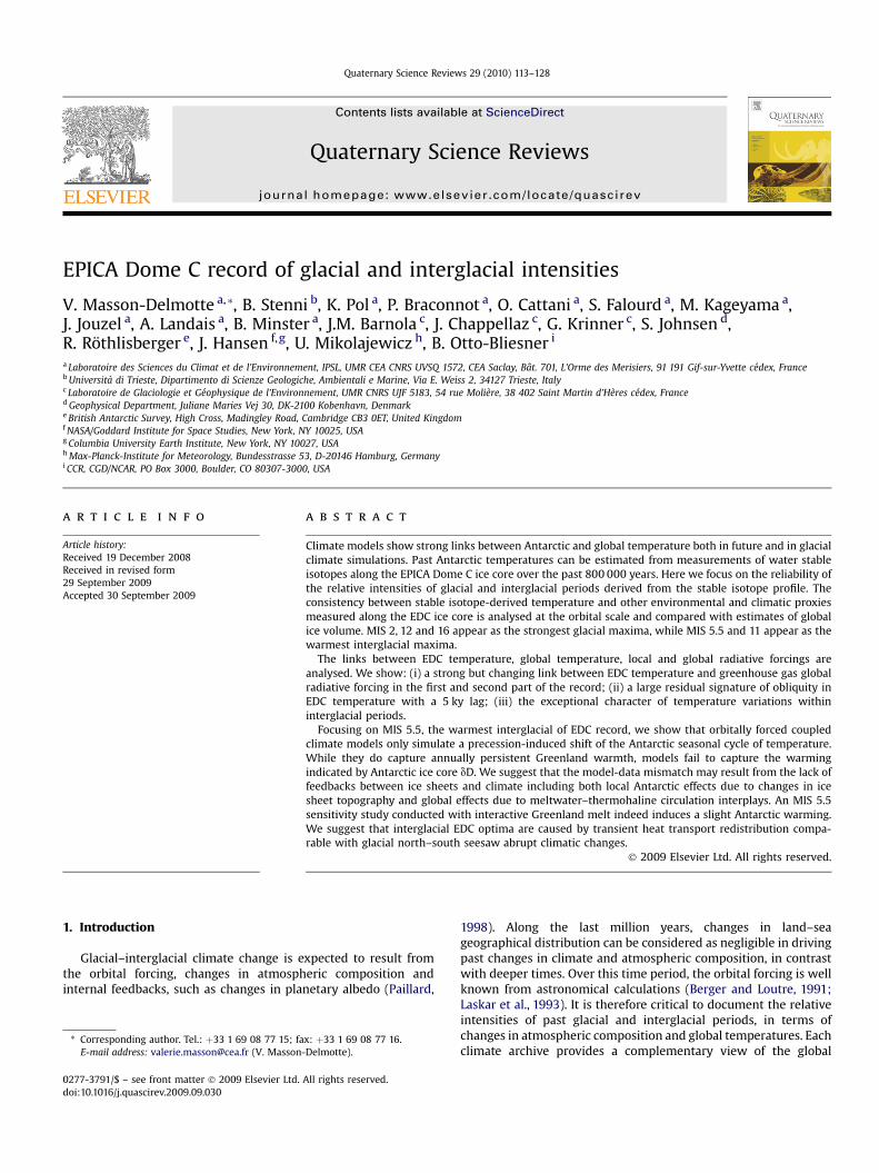
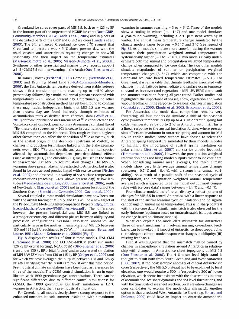
Fig. 1. Comparison of two methods to assess past EDC temperature based on EDC ice core dcomposition and a constant isotope–temperature slope. Red (Jouzel et al., 2007), same as gglaciological model used for the age scale, displayed in grey on the top panel (Parrenin et al.,levels.

are estimated from measurements of water stable isotopes alongthe EPICA EDC ice core over the past 800 000 years. We then discussthe consistency between stable isotope-derived temperature andother environmental and climatic proxies measured in the EDC icecore regarding the relative intensity of glacial and interglacialextrema.

Section 4 is dedicated to the links between radiative perturba-tions and climate and the new results from the EDC ice core. Wediscuss the weights of orbital frequencies in EDC temperature. Weanalyse the links between EDC temperature and greenhouse gasradiative forcing. We use climate models to discuss the relationshipbetween Antarctic and global temperature, highlighting the prob-lems of changes in local ice sheet elevation. A reconstruction of pastglobal temperature variations is compared to the simulations ofglobal temperature response to global radiative forcings estimatedfrom past changes in greenhouse gas concentrations and innorthern hemisphere glaciation.

As we show that EDC interglacial temperature variations cannotbe explained by a simple response to radiative forcing perturba-tions, we finally focus our discussion (Section 5) on the warmestinterglacial period identified in the EDC ice cores (MIS 5.5). Wecompare the response of climate models forced by changes inorbital configurations with observational constraints fromGreenland and Antarctica. We show that MIS 5.5 Antarctic warmthis not captured by the response of ocean and atmosphere dynamicsto orbital forcing and that other feedbacks involving the couplingwith the cryosphere must be at play.

2. Data

In this analysis, we use the available datasets measured andpreviously published, on the EPICA EDC3 age scale (Parrenin et al.,2007a). This age scale is generated by combining an accumulation andan ice flow model optimised using absolute age markers (Parreninet al., 2007b). For the time period from 300 to 800 kyr (thousands ofyears before present), the age scale is obtained from a glaciologicalinterpolation of precession age markers identified in EDC d18O of O2

(Dreyfus et al., 2007). The accuracy of the EDC3 age scale is estimatedto be w6 kyr from 130 kyr to 800 kyr. The EDC3 age scale is thereforeset up independently of the orbital properties of dD.

The dD measurements of the ice core are available on 55 cm icesections (‘‘bag samples’’) (Jouzel et al., 2007). Due to the combined

800600

P)

-150

-100

-50

0

50

)m(

egn

ahc

noit

avel

E

classical method + elevation correction classical method

D. Green, conventional approach taking into account past changes in sea water isotopicreen but also including a correction for ice sheet elevation changes derived from the2007b). Horizontal dashed lines show the average Holocene and Last Glacial Maximum

V. Masson-Delmotte et al. / Quaternary Science Reviews 29 (2010) 113–128 115

effects of lower glacial accumulation and ice thinning, this depthresolution corresponds to a temporal resolution of w20 yearsduring the Holocene, w50 years during MIS 2, w200 years duringMIS 11, w600 years during MIS 12 and w1000 years during theoldest glacial periods. As the average temporal spacing is w150years, we have re-sampled the data to a mean 200 year resolution.

The CO2 record discussed here is constructed with a stack ofconcentration measurements combined from the Vostok (Petitet al., 1999) and EPICA DC ice cores (Monnin et al., 2001;Siegenthaler et al., 2005; Luthi et al., 2008), transferred onto theEDC3 age scale. The methane profile is now continuously availablefrom the EDC ice core (Spahni et al., 2005; Loulergue et al., 2008).Hereafter, we use them either in terms of concentrations, or interms of radiative forcing, using a consensus conversion fromconcentration to radiative forcing (Joos, 2005). In the followingequations, atmospheric concentrations are expressed in ppmv forCO2 (respectively ppbv for CH4) and the pre-industrial referenceconcentration CO2,0 is 278 ppmv (respectively 742 ppbv for CH4,0);radiative forcings are expressed in W m�2; we neglect the correc-tion term accounting for the overlap between CH4 and N2Oabsorption bands. The global Radiative Forcing (RF) caused by thedifferent gases is then estimated by:

RFCO2¼ 5:35� ln

�½CO2��CO2;0

��

(1)

RFCH4¼ 0:036�

� ffiffiffiffiffiffiffiffiffiffiffiffi½CH4�

p�

ffiffiffiffiffiffiffiffiffiffiffiffiffiffiffiffi�CH4;0

�q �(2)

The temporal resolution of the records is variable. From theVostok data, the mean temporal interval between subsequent datais 1187�1080 years for CO2 (the largest gap between measure-ments is 8600 years). For Dome C, from 400 to 800 ka BP, the meantemporal interval between CO2 data is 684� 406 years (maximumspacing of 3525 years). For EDC CH4 data, the mean temporalinterval is 381�333 years (maximum spacing of 3460 years). Thebest documented periods have temporal resolutions up to 200years. In order to be consistent with the mean spacing of thedeuterium record, we have also re-sampled the stacked radiativeforcing record on a 200 year time step.

The dust flux is documented by 989 data points back to 740 kaBP, corresponding to a mean age distance of 750�1450 years(EPICA-Community-Members, 2004; Lambert et al., 2008). AsAntarctic ice core dust levels are log-normally distributed, we haveconsidered the logarithm of the dust flux as the function whichshould be most clearly related to the climate signal from dustsource areas (Petit and Delmonte, 2009).

By comparison, the temporal resolution of the chemical records(Wolff et al., 2006) is slightly higher than the dust profile resolution(a total of 1400 depths sampled). It was recently expanded to800 ka at 100 year resolution (Rothlisberger et al., 2008). Thechemical composition of the ice in terms of calcium, sodium andsulphate is published on a 2.2 m depth basis, corresponding to 1405depths and a mean temporal resolution of 530� 660 years. Forconsistency with the deuterium record, these profiles have alsobeen re-sampled to a 200 year time interval.

The accumulation rate is derived from the inverse glaciologicaldating method (Parrenin et al., 2007a), mainly as the result of anoptimised relationship with the deuterium content of the ice,which is supposedly related to the condensation temperature andthe moisture-holding capacity of the atmosphere. We haveused accumulation data at a 200 year time step to derive theatmospheric flux of aerosols from the observed concentrations ofnon-sea-salt calcium, sea salt sodium and dust. Note that while theaccuracy of the measurements of stable isotopes or greenhouse

gases is stable over glacials or interglacials, the very low levels ofdust and aerosol fluxes during interglacial periods make thediscussion of their variability within or between interglacials moredifficult due to the low signal to noise ratios (see the envelope ofthe profiles in Fig. 2).

In order to compare the EDC records with a northern hemi-sphere perspective, we have included in our comparison thenorthern hemisphere ice volume derived from the marinesediment signals after correction for deep water temperatureeffects (Bintanja et al., 2005) using benthic stacks (Lisiecki andRaymo, 2005).

Note that the time step of 200 years was selected based on theaverage resolution of deuterium data. We have repeated our anal-yses using a lower time resolution of 1000 years: our resultsregarding glacial and interglacial intensities are robust with respectto this sampling resolution.

3. Relative intensity of glacial and interglacial EDCtemperature changes

3.1. EDC temperature reconstructions

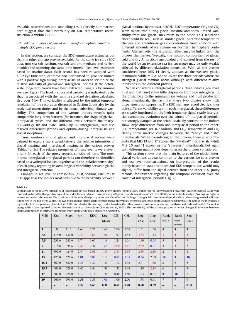
Fig. 1 shows different temperature reconstructions based on EDCstable isotope data. The detailed basis of temperature reconstruc-tions using ice core isotopic composition has been previously pub-lished (Jouzel et al., 2003; Masson-Delmotte et al., 2006b; Masson-Delmotte et al., 2008). Due to isotopic distillation processes, changesin central Antarctic snow dD are primarily driven by changes incondensation temperature. Past temperature reconstructions relyon the explicit assumptions of a constant relationship betweenmean condensation and surface temperatures (including a constantinversion strength). Available isotopic modelling studies show thatin central Antarctica the glacial–interglacial relationship betweensurface temperature and snow isotopic composition is similar to themodern spatial gradient (Jouzel et al., 2007). The EDC dD data haveto be corrected for sea water isotopic composition changes linkedwith ice volume formation (Bintanja et al., 2005). A first tempera-ture can then be estimated using the modern spatial isotope–temperature slope (Masson-Delmotte et al., 2008) and is referred toas ‘‘classical method’’. Several factors can have an additional impacton the temperature and are not accounted for in this ‘‘classical’’reconstruction:

1. In order to provide climate information which is independentof variations of local elevation, a ‘‘fixed elevation’’ temperaturereconstruction was recently produced (Jouzel et al., 2007). Pastelevation variations can be estimated from the accumulationand ice flow model used for EDC dating (Parrenin et al., 2007b).EDC elevation is reduced by up to 125 m during glacial periodsin response to reduced glacial accumulation, and enhanced byup to 45 m during ‘‘warm’’ interglacials such as MIS 5.5 (Fig. 1).The shapes and magnitudes of these modelled elevationchanges are comparable with other independent glaciologicalcalculations (Pollard and DeConto, 2009). In order to correct forelevation effects, we assume a constant lapse rate of 9 �C perkm based on modern spatial gradients. The hypothesis ofa constant lapse rate is supported by sensitivity studiesconducted with the LMDz model with different glacial ice sheetconfigurations (see Section 4.3). The glacial–interglacial EDCtemperature variations (at constant present-day altitude) areenhanced by w1 �C (w10%) when considering elevationchanges (Fig. 1). Early interglacials (before 420 ka) appearcooler than the most recent interglacials (since 420 ka), and theelevation correction enhances this temperature contrast (byw0.5 �C).

-2

0

2erutarepme

T

8006004002000

Age (ky BP)

-2

0

2

xulf

tsu

D

-2

0

2

OC

2

-2

0

2

HC

4

-2

0

2

xulf aCssn

-2

0

2

xulf

aNs

s

-2

0

2

level aeS

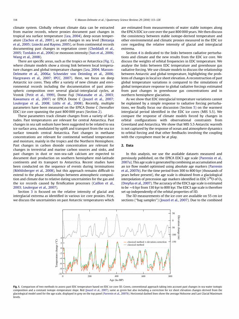
Fig. 2. Climate indices (in standard deviation units) derived from the ice core analyses and from marine sediments. Aerosol records (dust, calcium and sodium flux) were transformedwith a logarithm scale to have distributions comparable with other records. All time series were centered, normalised (average over 800 000 years zero, standard deviation 1, positiveanomaly during interglacials) and re-sampled with a time resolution of 200 years. In order to analyse the orbital scale features, running averages over 7000 years were performed. Themagnitude of suborbital variability (standard deviation within 7000 years) is displayed as the shaded envelop on each record. This apparent suborbital variability is obviouslydependent on the initial resolution of the records. Horizontal lines display plus or minus one standard deviation of the full indices. In the upper panel, the temperature index derivedfrom the Jouzel et al., (2007) temperature reconstruction (red) is compared with the average of all the other EDC climate indices displayed below (black line).

V. Masson-Delmotte et al. / Quaternary Science Reviews 29 (2010) 113–128116

2. Changes in evaporation conditions and moisture sources areexpected to impact the isotopic composition of the initial watervapour and the isotopic composition of the Antarctic snowfall(Vimeux et al., 2002). Deuterium excess data from EDC haveshown that EDC temperature reconstruction is robust withrespect to changes in moisture origin over the past climaticcycle (Stenni et al., 2010; Stenni et al., 2001).

3. Changes in precipitation seasonality and/or intermittency areexpected to play an important role in the sampling of climatesignals recorded in ice cores (Masson-Delmotte et al., 2006b;Timmermann et al., 2009). There is no proxy available to detectpast changes in snowfall seasonality. For present day, EDCaccumulation is dominated by a few randomly distributedsnowfall events (Gallee and Gorodetskaya, 2008). In the Vostokarea, a stake network showed that present-day accumulation isregularly distributed year round and mostly (75%) provided byclear sky precipitation (diamond dust) (Ekaykin, 2003). Climatemodels have been used to quantify the impact of past changesin snowfall seasonality. At the glacial–interglacial scale,modelling studies conducted with isotopic general circulationmodels support a stable central Antarctic isotope–temperatureslope and suggest that glacial–interglacial surface temperaturechanges based on Antarctic ice core stable isotope recordsshould be valid within �2 �C (Jouzel et al., 2003; Jouzel et al.,2007).

In order to assess the impact of changes in orbital configurationon precipitation seasonality aspects, we have analysed sensitivitysimulations conducted with the IPSL (Institut Pierre Simon Laplace)coupled climate model under pre-industrial boundary conditionsand with orbital configurations from present day, 6, 9, 115, 122 and126 kyr (thousands of years before present) spanning a range ofobliquity, precession and eccentricity configurations (Braconnotet al., 2008). For inland Antarctica (above 2500 m elevation), wehave calculated the annual mean temperature (average of monthlymean temperatures) and the precipitation weighted temperaturefrom monthly values of temperature and precipitation. The resultsfrom this coupled climate model indicate that the absolute value ofthe seasonal bias (difference between these two annual tempera-tures) is always lower than 0.5 �C. For 126 kyr, this result is furtherconfirmed by comparable results obtained with three other coupledclimate models (see Section 5). A 130 ka transient simulation hasrecently been conducted with the LOVECLIM model (Timmermann,pers. comm.), forced by astronomical, greenhouse gas, and ice sheetmodel based estimates of ice sheet topography and albedo. Incentral Antarctica, the precipitation weighted temperature is onaverage 1.2 �C above the annual mean surface temperature.Precession appears to modulate this bias by about �0.75 �C.

Considering uncertainties linked with changes in moistureorigin, local elevation, condensation versus surface temperaturevariations and by snowfall seasonality or intermittency, the

V. Masson-Delmotte et al. / Quaternary Science Reviews 29 (2010) 113–128 117

available observations and modelling results briefly summarizedhere suggest that the uncertainty on EDC temperature recon-struction is within 1–2 �C.

3.2. Relative intensity of glacial and interglacial optima based onmultiple EDC proxy records

In this section, we consider the EDC temperature estimates butalso the other climate proxies available for the same ice core (EDCdust, non-sea-salt calcium, sea salt sodium, methane and carbondioxide) and spanning the same time interval (sea level estimatesbased on marine data). Each record has been re-sampled witha 0.2 kyr time step, centered and normalised to produce indiceswith a positive sign during interglacials. In order to scrutinize therelative intensity of glacial and interglacial optima at the orbitalscale, long-term trends have been extracted using a 7 ky runningaverage (Fig. 2). The level of suborbital variability is indicated by theshading associated with the running standard deviation calculatedalso over 7 ky. This variability is affected by the initial temporalresolution of the records as discussed in Section 2, but also by theanalytical uncertainties and by the actual suborbital climate vari-ability. The comparison of the various indices reveals quitecomparable long-term features (for instance, the shape of glacial–interglacial cycles, and the different levels between the ‘‘early’’800–400 ky BP and ‘‘late’’ 400–0 ky BP interglacials), but alsomarked differences (trends and optima during interglacials andglacial inceptions).

Time windows around glacial and interglacial optima weredefined to explore more quantitatively the relative intensities ofglacial maxima and interglacial maxima in the various proxies(Tables 1a–1c). The relative intensities of these events were givena rank for each of the proxy records considered here. The mostintense interglacial and glacial periods can therefore be identifiedbased on a variety of indices, together with the ‘‘relative sensitivity’’of each proxy regarding its own range of variability between glacialand interglacial extrema.

Changes in sea level or aerosol flux (dust, sodium, calcium) atEDC appear as the indices most sensitive to the variability between

Table 1aComparison of the relative intensities of interglacial periods based on EDC proxy indicescentered, reduced (with a positive sign of the index for interglacials), sampled at a 200 yeintensities’’ at the orbital scale. The maximum of the smoothed proxy index was identifiedis reported in the table (red values, the two most intense interglacials for each proxy; blueis given for EDC temperature (Jouzel et al., 2007) and also for the averaged index based oninterglacials is also reported based on the estimate of past ice volume (Bintanja et al., 20interglacial periods is estimated using the inter-interglacial index standard deviation s.

MIS End Start D EDC

T

Log

(dust)

CO2

1 0.0 11.6 1.69 1.76 1.66 2.06

5.5 115.0 132.0 2.70 2.69 1.98 1.93

7.5 233.6 245.6 1.74 1.67 1.18 1.24

9 316.8 335.6 2.46 2.34 1.69 2.08

11 392.0 424.6 2.44 2.61 1.81 2.31

13 470.0 529.6 1.01 0.88 1.19 0.82

15.1 560.0 580.0 1.36 1.32 1.22 1.12

15.5 603.0 628.0 1.45 1.40 1.39 1.32

17 680.0 720.0 1.10 1.16 1.34 0.48

19 769.6 791.6 1.51 1.33 1.06 1.09

– – 0.59 0.63 0.31 0.61

glacial maxima. By contrast, EDC dD, EDC temperature, CH4 and CO2

seem to saturate during glacial maxima and show limited vari-ability from one glacial maximum to the other. This saturationeffect could be real, such as similar glacial Antarctic temperaturechanges and greenhouse gas concentrations could coincide withdifferent amounts of ice volume on northern hemisphere conti-nents. Alternatively, the saturation effect may be linked with theproxies themselves. Typically, the isotopic composition of glacialcold and dry Antarctica (surrounded and isolated from the rest ofthe world by an extensive sea ice coverage) may be only weaklyaffected by different glaciation intensities. With all the proxiesconsidered here, MIS 14 clearly appears as the weakest glacialmaximum, while MIS 2, 12 and 16 are the three periods where thestrongest glacial maxima occur, although with different relativeintensities in the different proxies.

When considering interglacial periods, three indices (sea level,dust and methane) show little dispersion from one interglacial tothe other. Due to the minimum ice volume and dust productionalong interglacials, the fact that these two proxies show littledispersion is not surprising. The EDC methane record clearly showsquite different variability within each interglacial; these differencesare clearly imprinted on the high frequency signal (early intergla-cial overshoots, evolution over the course of interglacial periods)but strongly damped at the orbital scale. By contrast, three indicesshow large differences from one interglacial period to the other:EDC temperature, sea salt sodium, and CO2. Temperature and CO2

clearly show marked changes between the ‘‘early’’ and ‘‘late’’interglacials. When considering all the proxies, there is no ambi-guity that MIS 13 and 17 appear the ‘‘weakest’’ interglacials, whileMIS 5.5 and 11 appear as the ‘‘strongest’’ interglacials, but againwith different magnitudes depending on the proxies considered.

This section shows that the main features of the glacial–inter-glacial variations appear common to the various ice core proxiesand sea level reconstructions. An interpretation of the resultspurely based on stable isotopes and EDC temperature would onlyslightly differ from the signal derived from the other EDC proxyrecords, for instance regarding the temporal evolution over thecourse of interglacial periods (Fig. 2).

(no unit). EDC initial records (converted to a logarithm scale for aerosol data) werear resolution and smoothed over 7000 years in order to analyse ‘‘average interglacialwithin large ‘‘interglacial’’ time intervals (end and start dates are given in ky BP) andvalues, the two less intense interglacials for each proxy). The rank of the interglacialsthe other proxies (dust, sodium, calcium, methane and carbon dioxide). The rank of05). The ‘‘sensitivity’’ of the various proxies to detect changes in intensity between

CH4 Log Log

(Na) (Ca)

Rank Rank

E DC T other

proxies

Sea

level

1.65 1.51 1.54 4 4 4

1.83 3.64 1.44 1 2 2

1.01 1.99 0.68 5 8 7

2.11 2.59 0.81 3 3 3

2.55 2.59 2.19 2 1 1

1.05 0.54 2.08 10 9 10

1.35 2.21 1.38 8 6 5

1.48 1.29 2.18 6 5 9

1.50 1.24 0.87 9 10 8

2.00 1.78 0.91 7 7 6

0.48 0.88 0.59 – – 0.30

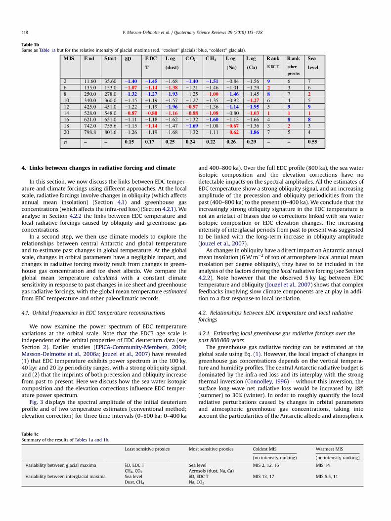
Table 1bSame as Table 1a but for the relative intensity of glacial maxima (red, ‘‘coolest’’ glacials; blue, ‘‘coldest’’ glacials).

M IS E nd Start D E DC

T

L og

(dust)

C O2 C H4 L og

(Na)

L og

(Ca)

R ank

E DC T

R ank

other

proxies

Sea

level

2 11.60 35.60 1.40 1.45 1.68 1.40 1.51 0.84 1.56 9 6 7 6 135.0 153.0 1.07 1.14 1.38 1.21 1.46 1.01 1.29 2 3 6 8 250.0 278.0 1.32 1.27 1.93 1.25 1.00 1.46 1.45 8 7 210 340.0 360.0 1.15 1.19 1.57 1.27 1.35 0.92 1.27 6 4 5 12 425.0 451.0 1.22 1.19 1.96 0.97 1.36 1.14 1.95 5 9 9 14 528.0 548.0 0.87 0.80 1.16 0.88 1.08 0.80 1.03 1 1 1 16 621.0 651.0 1.11 1.18 1.62 1.32 1.60 1.13 1.66 4 8 8 18 742.0 755.6 1.15 1.14 1.47 1.69 1.08 0.67 1.36 3 2 320 798.8 801.6 1.26 1.19 1.68 1.32 1.11 0.62 1.86 7 5 4

– – 0.15 0.17 0.25 0.24 0.22 0.26 0.29 – – 0.55

V. Masson-Delmotte et al. / Quaternary Science Reviews 29 (2010) 113–128118

4. Links between changes in radiative forcing and climate

In this section, we now discuss the links between EDC temper-ature and climate forcings using different approaches. At the localscale, radiative forcings involve changes in obliquity (which affectsannual mean insolation) (Section 4.1) and greenhouse gasconcentrations (which affects the infra-red loss) (Section 4.2.1). Weanalyse in Section 4.2.2 the links between EDC temperature andlocal radiative forcings caused by obliquity and greenhouse gasconcentrations.

In a second step, we then use climate models to explore therelationships between central Antarctic and global temperatureand to estimate past changes in global temperature. At the globalscale, changes in orbital parameters have a negligible impact, andchanges in radiative forcing mostly result from changes in green-house gas concentration and ice sheet albedo. We compare theglobal mean temperature calculated with a constant climatesensitivity in response to past changes in ice sheet and greenhousegas radiative forcings, with the global mean temperature estimatedfrom EDC temperature and other paleoclimatic records.

4.1. Orbital frequencies in EDC temperature reconstructions

We now examine the power spectrum of EDC temperaturevariations at the orbital scale. Note that the EDC3 age scale isindependent of the orbital properties of EDC deuterium data (seeSection 2). Earlier studies (EPICA-Community-Members, 2004;Masson-Delmotte et al., 2006a; Jouzel et al., 2007) have revealed(1) that EDC temperature exhibits power spectrum in the 100 ky,40 kyr and 20 ky periodicity ranges, with a strong obliquity signal,and (2) that the imprints of both precession and obliquity increasefrom past to present. Here we discuss how the sea water isotopiccomposition and the elevation corrections influence EDC temper-ature power spectrum.

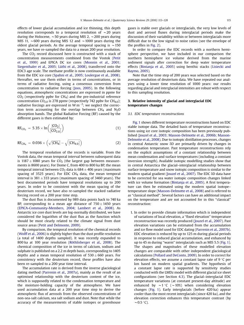
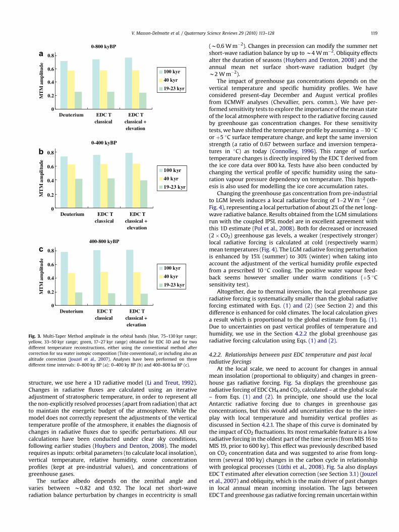
Fig. 3 displays the spectral amplitude of the initial deuteriumprofile and of two temperature estimates (conventional method;elevation correction) for three time intervals (0–800 ka; 0–400 ka

Table 1cSummary of the results of Tables 1a and 1b.

Least sensitive proxies Mos

Variability between glacial maxima dD, EDC T SeaCH4, CO2 Aero

Variability between interglacial maxima Sea level dD, EDust, CH4 Na, C

and 400–800 ka). Over the full EDC profile (800 ka), the sea waterisotopic composition and the elevation corrections have nodetectable impacts on the spectral amplitudes. All the estimates ofEDC temperature show a strong obliquity signal, and an increasingamplitude of the precession and obliquity periodicities from thepast (400–800 ka) to the present (0–400 ka). We conclude that theincreasingly strong obliquity signature in the EDC temperature isnot an artefact of biases due to corrections linked with sea waterisotopic composition or EDC elevation changes. The increasingintensity of interglacial periods from past to present was suggestedto be linked with the long-term increase in obliquity amplitude(Jouzel et al., 2007).

As changes in obliquity have a direct impact on Antarctic annualmean insolation (6 W m�2 of top of atmosphere local annual meaninsolation per degree obliquity), they have to be included in theanalysis of the factors driving the local radiative forcing (see Section4.2.2). Note however that the observed 5 ky lag between EDCtemperature and obliquity (Jouzel et al., 2007) shows that complexfeedbacks involving slow climate components are at play in addi-tion to a fast response to local insolation.

4.2. Relationships between EDC temperature and local radiativeforcings

4.2.1. Estimating local greenhouse gas radiative forcings over thepast 800 000 years

The greenhouse gas radiative forcing can be estimated at theglobal scale using Eq. (1). However, the local impact of changes ingreenhouse gas concentrations depends on the vertical tempera-ture and humidity profiles. The central Antarctic radiative budget isdominated by the infra-red loss and its interplay with the strongthermal inversion (Connolley, 1996) – without this inversion, thesurface long-wave net radiative loss would be increased by 18%(summer) to 30% (winter). In order to roughly quantify the localradiative perturbations caused by changes in orbital parametersand atmospheric greenhouse gas concentrations, taking intoaccount the particularities of the Antarctic albedo and atmospheric

t sensitive proxies Coldest MIS Warmest MIS

(no intensity ranking) (no intensity ranking)

level MIS 2, 12, 16 MIS 14sols (dust, Na, Ca)DC T MIS 13, 17 MIS 5.5, 11O2

0-800 kyBP

0

0.2

0.4

0.6

0.8

Deuterium EDC Tclassical

EDC Tclassical +elevation

ed

utilp

ma M

TM

100 kyr

40 kyr

19-23 kyr

0-400 kyBP

0

0.2

0.4

0.6

0.8

Deuterium EDC Tclassical

EDC Tclassical +elevation

dutilpma

MT

Me

100 kyr

40 kyr

19-23 kyr

400-800 kyBP

0

0.2

0.4

0.6

0.8

Deuterium EDC Tclassical

EDC Tclassical +elevation

ed

utilp

ma M

TM

100 kyr

40 kyr

19-23 kyr

a

b

c

Fig. 3. Multi-Taper Method amplitude in the orbital bands (blue, 75–130 kyr range;yellow, 33–50 kyr range; green, 17–27 kyr range) obtained for EDC dD and for twodifferent temperature reconstructions, either using the conventional method aftercorrection for sea water isotopic composition (Tsite conventional), or including also analtitude correction (Jouzel et al., 2007). Analyses have been performed on threedifferent time intervals: 0–800 ky BP (a); 0–400 ky BP (b) and 400–800 ka BP (c).

V. Masson-Delmotte et al. / Quaternary Science Reviews 29 (2010) 113–128 119

structure, we use here a 1D radiative model (Li and Treut, 1992).Changes in radiative fluxes are calculated using an iterativeadjustment of stratospheric temperature, in order to represent allthe non-explicitly resolved processes (apart from radiation) that actto maintain the energetic budget of the atmosphere. While themodel does not correctly represent the adjustments of the verticaltemperature profile of the atmosphere, it enables the diagnosis ofchanges in radiative fluxes due to specific perturbations. All ourcalculations have been conducted under clear sky conditions,following earlier studies (Huybers and Denton, 2008). The modelrequires as inputs: orbital parameters (to calculate local insolation),vertical temperature, relative humidity, ozone concentrationprofiles (kept at pre-industrial values), and concentrations ofgreenhouse gases.

The surface albedo depends on the zenithal angle andvaries between w0.82 and 0.92. The local net short-waveradiation balance perturbation by changes in eccentricity is small

(w0.6 W m�2). Changes in precession can modify the summer netshort-wave radiation balance by up to w4 W m�2. Obliquity effectsalter the duration of seasons (Huybers and Denton, 2008) and theannual mean net surface short-wave radiation budget (byw2 W m�2).

The impact of greenhouse gas concentrations depends on thevertical temperature and specific humidity profiles. We haveconsidered present-day December and August vertical profilesfrom ECMWF analyses (Chevallier, pers. comm.). We have per-formed sensitivity tests to explore the importance of the mean stateof the local atmosphere with respect to the radiative forcing causedby greenhouse gas concentration changes. For these sensitivitytests, we have shifted the temperature profile by assuming a�10 �Cor þ5 �C surface temperature change, and kept the same inversionstrength (a ratio of 0.67 between surface and inversion tempera-tures in �C) as today (Connolley, 1996). This range of surfacetemperature changes is directly inspired by the EDC T derived fromthe ice core data over 800 ka. Tests have also been conducted bychanging the vertical profile of specific humidity using the satu-ration vapour pressure dependency on temperature. This hypoth-esis is also used for modelling the ice core accumulation rates.

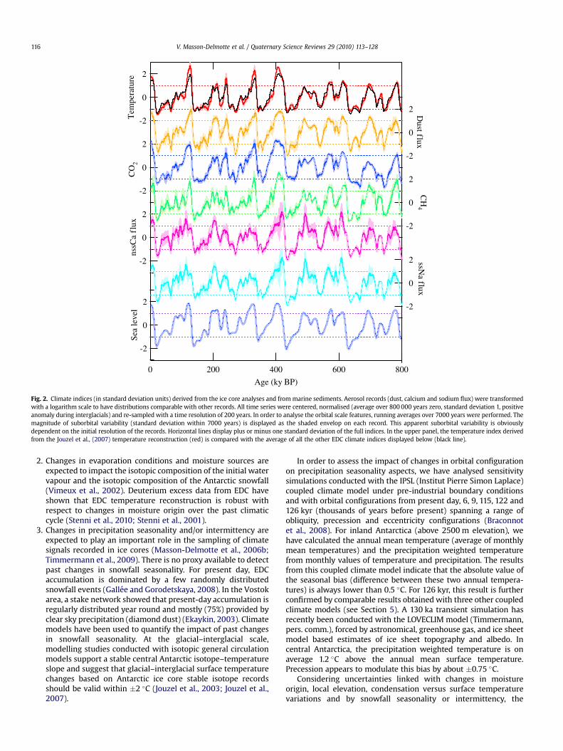
Changing the greenhouse gas concentration from pre-industrialto LGM levels induces a local radiative forcing of 1–2 W m�2 (seeFig. 4), representing a local perturbation of about 2% of the net long-wave radiative balance. Results obtained from the LGM simulationsrun with the coupled IPSL model are in excellent agreement withthis 1D estimate (Pol et al., 2008). Both for decreased or increased(2� CO2) greenhouse gas levels, a weaker (respectively stronger)local radiative forcing is calculated at cold (respectively warm)mean temperatures (Fig. 4). The LGM radiative forcing perturbationis enhanced by 15% (summer) to 30% (winter) when taking intoaccount the adjustment of the vertical humidity profile expectedfrom a prescribed 10 �C cooling. The positive water vapour feed-back seems however smaller under warm conditions (þ5 �Csensitivity test).

Altogether, due to thermal inversion, the local greenhouse gasradiative forcing is systematically smaller than the global radiativeforcing estimated with Eqs. (1) and (2) (see Section 2) and thisdifference is enhanced for cold climates. The local calculation givesa result which is proportional to the global estimate from Eq. (1).Due to uncertainties on past vertical profiles of temperature andhumidity, we use in the Section 4.2.2 the global greenhouse gasradiative forcing calculation using Eqs. (1) and (2).

4.2.2. Relationships between past EDC temperature and past localradiative forcings

At the local scale, we need to account for changes in annualmean insolation (proportional to obliquity) and changes in green-house gas radiative forcing. Fig. 5a displays the greenhouse gasradiative forcing of EDC CH4 and CO2, calculated – at the global scale– from Eqs. (1) and (2). In principle, one should use the localAntarctic radiative forcing due to changes in greenhouse gasconcentrations, but this would add uncertainties due to the inter-play with local temperature and humidity vertical profiles asdiscussed in Section 4.2.1. The shape of this curve is dominated bythe impact of CO2 fluctuations. Its most remarkable feature is a lowradiative forcing in the oldest part of the time series (from MIS 16 toMIS 19, prior to 600 ky). This effect was previously described basedon CO2 concentration data and was suggested to arise from long-term (several 100 ky) changes in the carbon cycle in relationshipwith geological processes (Luthi et al., 2008). Fig. 5a also displaysEDC T estimated after elevation correction (see Section 3.1) (Jouzelet al., 2007) and obliquity, which is the main driver of past changesin local annual mean incoming insolation. The lags betweenEDC T and greenhouse gas radiative forcing remain uncertain within

-3

-2

-1

0

1

2

3

4

LMG

DP

LMG

+5

LMG

01-q01-

MGL

DP2OCx2

5+2OCx2

q5+2OCx2

)²m/

W(gnicrof

evitaidaR

August

December

Global

Fig. 4. EDC radiative forcing calculations. The radiative budgets are calculated with a 1D radiative transfer model forced by prescribed vertical profiles of temperature and specifichumidity, and different concentrations in greenhouse gases (pre-industrial, 280 ppm of CO2, 580 ppb of CH4, 270 ppb of N2O; LGM, 180 ppm of CO2, 390 ppb of CH4, 220 ppb of N2O;2� CO2, 560 ppm, other gases at their pre-industrial levels). A fixed pre-industrial ozone concentration profile is used. The present-day vertical temperature profiles are obtainedfrom ECMWF analyses for December and August. Sensitivity tests are conducted by shifting the surface temperature by �10 or þ5 �C, assuming constant inversion strength, and bycalculating associated humidity (q) profiles (using the saturation vapour pressure–temperature relationship). Vertical bars display changes in radiative forcing changes betweenpre-industrial greenhouse gas concentrations and LGM or 2� CO2 greenhouse gas concentrations, for different hypotheses of vertical temperature and humidity profiles (PD,present day; þ5 or �10 �C perturbations; ‘‘q’’ indicates a calculation of specific humidity feedback) and for two seasons (August, grey and December, white). For comparison, globalannual radiative forcing calculations from Eq. (1) are displayed (shaded bars).

V. Masson-Delmotte et al. / Quaternary Science Reviews 29 (2010) 113–128120

a few centuries due to gas age–ice age differences (Dreyfus et al.,2010).

Fig. 5b displays the relationship between EDC T and the green-house gas radiative forcing. The colour scale is used to show thetemporal evolution, ranging from blue (800 ky BP) to red (presentday), as indicated on the EDC T profile (Fig. 5a). The relationshipbetween EDC T and greenhouse radiative forcing exhibits a crescent(convex) shape. During glacial minima, the slope betweentemperature and radiative forcing is very small, while it appearslarger for the warmest interglacials. The relationship is notsymmetric between glacial inceptions and terminations. It exhibitsa hysteresis behaviour with values above the linear fit for termi-nations and below the linear fit for inceptions. Interglacial periodsexhibit a complete decoupling of the greenhouse gas radiativeforcing and EDC T (Fig. 5a). As a first approximation, we can usea linear relationship between EDC T and radiative forcing, witha slope of 3.9 �C per W m�2 (R2¼ 0.80), or a parabolic fit (R2¼ 0.82)(Fig. 5b). An F-test conducted on the residuals confirms lowerunexplained variance for the parabolic fit than for the linear fit(p¼ 2�10�5). The ‘‘crescent’’ (convex) shape is robust with respectto the method used to estimate the local greenhouse gas radiativeforcing (using Eqs. (1) and (2)) or more precise local radiativecalculations leading to a smaller radiative forcing under colderconditions, see Section 4.2.1.

While EDC T shows a strong obliquity signal (see Section 4.1),the linear relationship between EDC T and obliquity is small butsignificant (95% confidence level), with a slope of 1 �C per degreeobliquity (R2¼ 0.1). Note that a maximum R2 of 0.2 is reached usinga lag of 5 ky, leading to a slope of 2.1 �C per degree obliquity. Here,we explore the impact of instantaneous annual mean radiativeforcings on Antarctic temperature and therefore ignore this lag. Amultiple linear regression leads to a reconstructed EDC T whichcaptures 82% of EDC T variance (93% through changes in green-house gas radiative forcing and 7% due to changes in obliquity). Inorder to identify the part of EDC T which cannot be explained bya simple linear response to changes in greenhouse gas radiativeforcing and in-phase obliquity, we have displayed the residual ofEDC T (grey line, Fig. 5a). The magnitude and shape of this residualis unchanged when considering obliquity or not, or when consid-ering a linear or parabolic link with greenhouse gas radiative

forcing, or when using Eqs. (1) and (2) or local estimates ofgreenhouse gas radiative forcing (see Section 4.2.1). The result isnot sensitive to the corrections for past changes in EDC elevation. Apart of the sharp variations of this residual temperature cannot bediscussed as they arise from the phase lags between temperatureand greenhouse gas variations during terminations or inceptions.The millennial variability reflects the Antarctic Isotopic Maxima(AIM), which are the Antarctic temperature counter-part of Dans-gaard–Oeschger variability (EPICA-Community-Members, 2006;Jouzel et al., 2007; Loulergue et al., 2008). AIM events are under-stood to be driven by reorganisations in meridional oceanic circu-lation (Stocker and Johnsen, 2003) and correlate with parallelmillennial variations in atmospheric CO2 concentration, reachingw20 ppmv (Ahn and Brook, 2008) (Schmittner and Galbraith,2008). These millennial CO2 variations are not fully resolved in thecurrent Vostok and EDC low resolution profiles. We therefore focuson the multi-millenial variations, highlighted in red using an orbitalband Gaussian pass filter (see caption of Fig. 5a).

First, this residual reveals a long-term trend. From about 800 kyBP to about 380 ky BP, the EDC temperature residual shows a slowdecreasing trend, followed by a slow increasing trend towards thepresent day. These slow trends were not obvious in the profiles ofgreenhouse gas concentrations, radiative forcing, or the initial EDCtemperature. This trend cannot be explained by the currentunderstanding of past changes in ice sheet elevation (Pollard andDeConto, 2009). This result suggests that long-term processes alterthe coupling between greenhouse radiative forcing and tempera-ture. In other words, the response of Antarctic temperature tochanges in radiative forcing may vary over a time scale of w400 ky.The cause for such long-term fluctuations remains to beunderstood.

Secondly, this residual reveals a strong obliquity component,which can be seen from the comparison of its orbital component(red line) with the fluctuations of obliquity (yellow line) (Fig. 5a).Most of the obliquity component in EDC T is not due to the local andinstantaneous response to Antarctic insolation change (or to theobliquity component of the greenhouse gas radiative forcing) but toa delayed response (with a lag of 5 ky with respect to obliquity).There is therefore a strong obliquity component in the residual. Thecoherency of the residual with obliquity is minimal for the period

-4

-2

0

2

4

)C°

( lau

dise

r T

8007006005004003002001000Age EDC3 (ky BP)

-10

-5

0

5

)C°( yla

mona erutarepmet

CD

E

-3

-2

-1

0

1

m.W(

gni

crof

evi

taid

aR

2-)

24.0

23.5

23.0

)°( ytiuqilbO

-4

-2

0

2

)C°

( lau

dise

r T

28

26

)C°

( TS

S B6

08P

DO

24

22

)C°(

TSS B648

PD

O

-12

-10

-8

-6

-4

-2

0

2

4

6

)C°( yla

mona erutarepmet

CD

E

-3 -2 -1 0 1

RF (W.m-2)

a

b

Fig. 5. (a). Change in radiative forcing due to CO2 and CH4 calculated using Vostok andEDC data (Petit et al., 1999; Loulergue et al., 2008; Luthi et al., 2008) using the formulaof Joos (2005) (top panel, grey line). EDC temperature with elevation correction (Jouzelet al., 2007) (colour scale reflecting the temporal evolution from past to present, blueto red). A regression is calculated between EDC T and radiative forcing (Fig. 5a). Theresidual part of EDC temperature that cannot be explained by a multiple linear modelconsidering greenhouse gas radiative forcing and obliquity (dark grey, using a para-bolic regression; red line, orbital long-term component of the regression residual). Thisorbital component (red line) is superimposed on the obliquity fluctuations (yellowline). SST records from the Pacific Ocean are displayed in the lowest panel, based onalkenones for ODP846B (thin grey line, original data; thick light blue, low pass filter)(Lawrence et al., 2006) and on Mg/Ca for ODP806B (thin light blue line, original data;thick dark blue, low pass filter) (Medina-Elizalde and Lea, 2005). (b). Change in EDCtemperature (Jouzel et al., 2007) (vertical axis, �C) as a function of the radiative forcingdue to CO2 and CH4 calculated using Vostok and EDC data (Petit et al., 1999; Loulergueet al., 2008; Luthi et al., 2008) using the formula of Joos (2005) (Eqs. (1) and (2)). Thecolour scale reflects the temporal evolution from past to present, blue to red as inFig. 6b. Linear (dashed line) and parabolic (solid black line) regressions are displayed.

V. Masson-Delmotte et al. / Quaternary Science Reviews 29 (2010) 113–128 121

between 350 and 400 ky, a period poorly constrained in the EDC3age scale (Dreyfus et al., 2007; Parrenin et al., 2007a), questioningthe accuracy of the EDC3 age scale for MIS 10–12. This analysisreveals that the large signature of obliquity in EDC temperature(Jouzel et al., 2007) cannot solely be attributed to the obliquitycomponent of the greenhouse gas radiative forcing or to instanta-neous local incoming solar radiation. The fact that the obliquitysignal is in phase in equatorial Pacific sea surface temperaturerecords (Medina-Elizalde and Lea, 2005; Lawrence et al., 2006) andin Antarctica suggests coupling mechanisms between low and highlatitudes, as also observed at the multi-decadal time scale (Ekaykinet al., 2004). There are also long-term trends in the equatorialPacific sea surface temperatures between 800 and 400 ky BP whichsuggest that this low–high latitude coupling may also be at play onlonger time scales (Fig. 5a).

While levels of greenhouse gas radiative forcing and obliquitycan account for different ‘‘mean levels’’ of interglacials, this is notthe case for the EDC T evolution over the course of interglacialperiods. Early interglacial optima cannot be explained by a simpleresponse to changes in local radiative forcings.

4.3. Relationships between EDC temperature and globaltemperature

One may want to use EDC greenhouse gas radiative forcings,infer global temperature from EDC temperature, and finally discussglobal climate sensitivity based on glacial–interglacial changes,following the pioneer approach conducted for Vostok (Genthonet al., 1987). Based on Last Glacial Maximum (LGM) PMIP (Paleo-climate Modelling Intercomparison Project), climate model simu-lations, the glacial–interglacial change in central Antarctictemperature appears to be linked with global temperature change,with an amplifying factor of w2 (Masson-Delmotte et al., 2006a)(Fig. 6). Under present-day boundary conditions, and in response toincreased CO2 levels, coupled climate models also exhibit a linearrelationship between central Antarctic and global temperaturechanges (Fig. 6), albeit with a slope of w1.2. A 130 ka simulationconducted with the intermediate complexity model LOVECLIM (seeSection 3.1) also shows strong correlation between Antarctic andglobal temperature, with a slope of w2 (Timmermann, pers.comm.).

This result can be compared with modelling studies conductedwith different versions of the same climate model with differentequilibrium CO2 sensitivities, mostly comparing their results for theLGM and for future climate change. An intermediate complexityclimate model (Schneider von Deimling et al., 2006) showed anLGM Antarctic cooling of 2.5 �C per �C of climate sensitivity(therefore 7.5 �C for the most plausible 3 �C equilibrium sensi-tivity). Studies with a general circulation model (Hargreaves et al.,2007) also highlighted a strong link between the model sensitivityand its Antarctic temperature response. Finally a linear relationshipbetween LGM Antarctic cooling and CO2-induced Antarctic warm-ing was demonstrated with four coupled climate models (Crucifix,2006) (see his Fig. 2).

State-of-the-art PMIP2 (Paleoclimate Modelling Intercompar-ison Project, Phase 2) coupled climate models simulate a globalLGM cooling of 4.6� 0.9 �C and a central Antarctic annual meansurface air temperature changes of 8.8� 3.6 �C (Fig. 6). The simu-lated Antarctic temperature change seems at first sight in very goodagreement with EDC T reconstruction (Fig. 1). However, half of thesimulated glacial–interglacial Antarctic temperature magnitude isan artefact of the prescribed PMIP2 glacial boundary conditions.Whereas all ice sheet glaciological models suggest that the LGMtopography was w100–200 m lower than at present in central EastAntarctica, because of the lower glacial accumulation (see Section

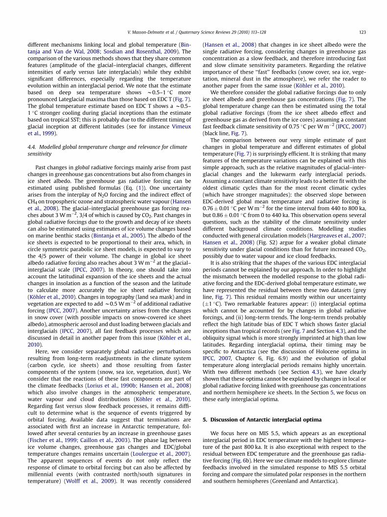
Fig. 7. Calculation of global radiative forcings (Hansen et al., 2008) associated withslow feedback processes involving past changes in carbon cycle (global greenhouse gasconcentrations using only continuous records of EDC and Vostok CO2 and CH4) (green)and in ice sheet extent, deriving ice sheet extent as a function of an estimate ofnorthern and southern hemisphere ice volume using global ice volume estimates fromBintanja et al. (2005) (in light blue). The global temperature change is estimated usingeither a ratio of 1/2 with respect to EDC temperature (red, with a �1 �C uncertaintyshading), a ratio of 2/3 from equatorial Pacific SST (Medina-Elizalde and Lea, 2005)(pink) or deep ocean temperature (blue) (Zachos et al., 2001) (light blue) (Bintanjaet al., 2005). The global temperature change is calculated using the past ice sheetalbedo and greenhouse gas radiative forcings and the fast feedback global temperaturesensitivity of 0.75 �C per W m�2 (Hansen et al., 2008) (black). The residual between theestimated global temperature using EDC temperature and the modelled globaltemperature is displayed in grey. Marine Isotopic Stages associated with strongresiduals are displayed.

0

2

4

6

8

10

12

14

16

18

20

0 2 4 6 8 10

Global T (°C)

)C°(

T citcratn

A lartne

C

IPCC 2x

IPCC 4x

PMIP1

PMIP2

Sensitivity

Fig. 6. Comparison between Central Antarctic (area above 2500 m elevation) andglobal surface air temperature changes simulated by coupled climate models inresponse to sensitivity simulations to CO2 increase (orange, CMIP 2� CO2 minuscontrol; red, 4� CO2 minus control) and in response to Last Glacial Maximumboundary conditions (in blue, control minus PMIP1; in green, control minus PMIP2LGM boundary conditions). Datasets for CMIP simulations are similar to those informearlier studies (Masson-Delmotte et al., 2006b). Datasets for PMIP2 simulations havebeen updated from these references to include 5 more model results (PMIP databasehttp://pmip2.lsce.ipsl.fr/on date of November 25th, 2008). Sensitivity tests are LGMsimulations conducted with the LMDZ model with ICEG5 ice sheet topography (uppercircle) and with the modern Antarctic topography (lower circle). The dashed linesshow slopes of 1:1 and 2:1.

V. Masson-Delmotte et al. / Quaternary Science Reviews 29 (2010) 113–128122

3.1 and Fig. 1), the LGM ICE5G topography (Peltier, 2004) interpo-lated in PMIP simulations is w400 m above present day in centralAntarctica. Using the modern spatial altitude–surface air temper-ature gradient of w10 �C per km, we can roughly estimate that theprescribed topography should account for a w4 �C Antarctic cool-ing at LGM, almost half of the simulated magnitude.

A specific sensitivity study has been conducted with the LMDzatmospheric general circulation model (Hourdin et al., 2006). Withthis model, three different LGM simulations were run. All simula-tions include changes in orbital parameters and greenhouse gasconcentrations following PMIP recommendations (Joussaume andTaylor, 1995). The first one (CLIMAP-ICE5G) is a conventional PMIP1type simulation (Joussaume and Taylor, 1995) using CLIMAP SST(CLIMAP, 1981) and ICE5G ice sheets (Peltier, 2004). The secondsimulation (GERSONDE-ICE5G) is a sensitivity test to the southernocean surface boundary conditions performed using new recon-structions (Gersonde et al., 2005). The third simulation (GER-SONDE-MODERN) is a sensitivity test to the Antarctic ice sheettopography performed using the present-day Antarctic ice sheetwith the same ocean surface data (Gersonde et al., 2005). Thesesimulations show no significant impacts of southern boundaryconditions on global mean and Antarctic temperature changes (notshown), coherent with limited impacts of austral sea ice albedofound in PMIP2 simulations at the LGM (Braconnot et al., 2007). Thecomparison between annual mean temperature and precipitationweighted temperature changes confirms earlier AGCM studiessuggesting limited (<1.3 �C) LGM central Antarctic seasonalityeffects (Krinner et al., 1997; Krinner and Werner, 2003; Masson-Delmotte et al., 2006a). By contrast, the impact of changes in icesheet topography is striking. The ICE5G change in topography doesnot affect the seasonality of precipitation but accounts for a simu-lated temperature change at Dome C of 3.6 �C (blue circles, Fig. 6),almost half of the LGM-control magnitude. This sensitivity studyconfirms our initial prediction that almost half of the PMIP simu-lated glacial–interglacial central Antarctic temperature may bean artefact of the prescribed LGM ice sheet topography (Masson-Delmotte et al., 2006a).

The uncertainty linked with the prescribed PMIP2 Antarctic icesheet topography limits the model-data comparison, but mostmodel simulations (Fig. 4) clearly show a strong link between thesimulated Antarctic and the simulated global mean temperatureboth for past and future climate boundary conditions. Followingearlier studies (Lorius et al., 1990a; Hansen et al., 2008), we assumethat past global mean temperature changes can be estimated usingpast EDC temperature changes. Our fixed point is the LGM forwhich global ocean temperature databases and climate modelsimulations are available (Otto-Bliesner, 2009).

We therefore use a slope of 1/2 to estimate past changes inglobal temperature from changes in EDC T (Fig. 7). This scaling maybe inappropriate for interglacial periods, for which increased CO2

climate change simulations suggest a slope of 1/1.2 (Fig. 6). Thisscaling is also problematic for millennial bipolar seesaw eventssuch as Antarctic Isotopic Maxima (EPICA-Community-Members,2006). Due to the uncertainties on EDC T reconstructions (typically2 �C), the magnitude of millennial variability (typically 2 �C), andthe uncertainty on the slope between Antarctic and globaltemperature (between 1.16 for future climate and 2 for LGM), weestimate an uncertainty of about 1–2 �C on the reconstructed globalmean temperature (1 �C light red shading, Fig. 7).

There is no available global synthesis of temperature recordsspanning the past 800 000 years from other latitudes. Other esti-mates of past global temperature changes have been previouslypublished using deep ocean temperature (Zachos et al., 2001;Bintanja et al., 2005) or tropical Sea Surface Temperature (SST)records (Lea, 2004; Medina-Elizalde and Lea, 2005; Hansen et al.,2008) also scaled for the LGM with a slope of 2/3 (see theircomparison on Fig. 7). Detailed comparisons are limited by theresolutions of the records (much higher for EDC), age scale and lagsuncertainties. Each of these estimates is of course biased by theproxy records potentially affected by seasonality effects and by the

V. Masson-Delmotte et al. / Quaternary Science Reviews 29 (2010) 113–128 123

different mechanisms linking local and global temperature (Bin-tanja and Van de Wal, 2008; Sosdian and Rosenthal, 2009). Thecomparison of the various methods shows that they share commonfeatures (amplitude of the glacial–interglacial changes, differentintensities of early versus late interglacials) while they exhibitsignificant differences, especially regarding the temperatureevolution within an interglacial period. We note that the estimatebased on deep sea temperature shows w0.5–1 �C morepronounced Lateglacial maxima than those based on EDC T (Fig. 7).The global temperature estimate based on EDC T shows a w0.5–1 �C stronger cooling during glacial inceptions than the estimatebased on tropical SST; this is probably due to the different timing ofglacial inception at different latitudes (see for instance Vimeuxet al., 1999).

4.4. Modelled global temperature change and relevance for climatesensitivity

Past changes in global radiative forcings mainly arise from pastchanges in greenhouse gas concentrations but also from changes inice sheet albedo. The greenhouse gas radiative forcing can beestimated using published formulas (Eq. (1)). One uncertaintyarises from the interplay of N2O forcing and the indirect effect ofCH4 on tropospheric ozone and stratospheric water vapour (Hansenet al., 2008). The glacial–interglacial greenhouse gas forcing rea-ches about 3 W m�2, 3/4 of which is caused by CO2. Past changes inglobal radiative forcings due to the growth and decay of ice sheetscan also be estimated using estimates of ice volume changes basedon marine benthic stacks (Bintanja et al., 2005). The albedo of theice sheets is expected to be proportional to their area, which, incircle symmetric parabolic ice sheet models, is expected to vary tothe 4/5 power of their volume. The change in global ice sheetalbedo radiative forcing also reaches about 3 W m�2 at the glacial–interglacial scale (IPCC, 2007). In theory, one should take intoaccount the latitudinal expansion of the ice sheets and the actualchanges in insolation as a function of the season and the latitudeto calculate more accurately the ice sheet radiative forcing(Kohler et al., 2010). Changes in topography (land sea mask) and invegetation are expected to add w0.5 W m�2 of additional radiativeforcing (IPCC, 2007). Another uncertainty arises from the changesin snow cover (with possible impacts on snow-covered ice sheetalbedo), atmospheric aerosol and dust loading between glacials andinterglacials (IPCC, 2007), all fast feedback processes which arediscussed in detail in another paper from this issue (Kohler et al.,2010).

Here, we consider separately global radiative perturbationsresulting from long-term readjustments in the climate system(carbon cycle, ice sheets) and those resulting from fastercomponents of the system (snow, sea ice, vegetation, dust). Weconsider that the reactions of these fast components are part ofthe climate feedbacks (Lorius et al., 1990b; Hansen et al., 2008)which also involve changes in the atmospheric temperature,water vapour and cloud distributions (Kohler et al., 2010).Regarding fast versus slow feedback processes, it remains diffi-cult to determine what is the sequence of events triggered byorbital forcing. Available data suggest that terminations areassociated with first an increase in Antarctic temperature, fol-lowed after several centuries by an increase in greenhouse gases(Fischer et al., 1999; Caillon et al., 2003). The phase lag betweenice volume changes, greenhouse gas changes and EDC/globaltemperature changes remains uncertain (Loulergue et al., 2007).The apparent sequences of events do not only reflect theresponse of climate to orbital forcing but can also be affected bymillennial events (with contrasted north/south signatures intemperature) (Wolff et al., 2009). It was recently considered

(Hansen et al., 2008) that changes in ice sheet albedo were thesingle radiative forcing, considering changes in greenhouse gasconcentration as a slow feedback, and therefore introducing fastand slow climate sensitivity parameters. Regarding the relativeimportance of these ‘‘fast’’ feedbacks (snow cover, sea ice, vege-tation, mineral dust in the atmosphere), we refer the reader toanother paper from the same issue (Kohler et al., 2010).

We therefore consider the global radiative forcings due to onlyice sheet albedo and greenhouse gas concentrations (Fig. 7). Theglobal temperature change can then be estimated using the totalglobal radiative forcings (from the ice sheet albedo effect andgreenhouse gas as derived from the ice cores) assuming a constantfast feedback climate sensitivity of 0.75 �C per W m�2 (IPCC, 2007)(black line, Fig. 7).

The comparison between our very simple estimate of pastchanges in global temperature and different estimates of globaltemperature (Fig. 7) is surprisingly efficient. It is striking that manyfeatures of the temperature variations can be explained with thissimple approach, such as the relative magnitudes of glacial–inter-glacial changes and the lukewarm early interglacial periods.Assuming a constant climate sensitivity leads to a better fit with theoldest climatic cycles than for the most recent climatic cycles(which have stronger magnitudes): the observed slope betweenEDC-derived global mean temperature and radiative forcing is0.76� 0.01 �C per W m�2 for the time interval from 440 to 800 ka,but 0.86� 0.01 �C from 0 to 440 ka. This observation opens severalquestions, such as the stability of the climate sensitivity underdifferent background climate conditions. Modelling studiesconducted with general circulation models (Hargreaves et al., 2007;Hansen et al., 2008) (Fig. S2) argue for a weaker global climatesensitivity under glacial conditions than for future increased CO2,possibly due to water vapour and ice cloud feedbacks.

It is also striking that the shapes of the various EDC interglacialperiods cannot be explained by our approach. In order to highlightthe mismatch between the modelled response to the global radi-ative forcing and the EDC-derived global temperature estimate, wehave represented the residual between these two datasets (greyline, Fig. 7). This residual remains mostly within our uncertainty(�1 �C). Two remarkable features appear: (i) interglacial optimawhich cannot be accounted for by changes in global radiativeforcings, and (ii) long-term trends. The long-term trends probablyreflect the high latitude bias of EDC T which shows faster glacialinceptions than tropical records (see Fig. 7 and Section 4.3), and theobliquity signal which is more strongly imprinted at high than lowlatitudes. Regarding interglacial optima, their timing may bespecific to Antarctica (see the discussion of Holocene optima inIPCC, 2007, Chapter 6, Fig. 6.9) and the evolution of globaltemperature along interglacial periods remains highly uncertain.With two different methods (see Section 4.3), we have clearlyshown that these optima cannot be explained by changes in local orglobal radiative forcing linked with greenhouse gas concentrationsand northern hemisphere ice sheets. In the Section 5, we focus onthese early interglacial optima.

5. Discussion of Antarctic interglacial optima

We focus here on MIS 5.5, which appears as an exceptionalinterglacial period in EDC temperature with the highest tempera-ture of the past 800 ka. It is also exceptional with respect to theresidual between EDC temperature and the greenhouse gas radia-tive forcing (Fig. 6b). Here we use climate models to explore climatefeedbacks involved in the simulated response to MIS 5.5 orbitalforcing and compare the simulated polar responses in the northernand southern hemispheres (Greenland and Antarctica).

V. Masson-Delmotte et al. / Quaternary Science Reviews 29 (2010) 113–128124

Greenland ice cores cover parts of MIS 5.5, back to w123 ky BPin the bottom part of the unperturbed NGRIP ice core (NorthGRIP-Community-Members, 2004; Landais et al., 2005) and in pieces ofthe disturbed parts of the GRIP and GISP2 ice cores (Landais et al.,2003). The 3& enhanced Greenland ice core d18O suggest thatGreenland temperature was w5 �C above present day, with theusual caveats and uncertainties regarding changes in snowfallseasonality and their impact on the temperature estimates(Masson-Delmotte et al., 2005; Masson-Delmotte et al., 2006b).Syntheses of other terrestrial and marine proxy records supporta 3–5 �C MIS 5.5 summer warming in the Arctic (Otto-Bliesner et al.,2006).

In Dome C, Vostok (Petit et al., 1999), Dome Fuji (Watanabe et al.,2003) and Dronning Maud Land (EPICA-Community-Members,2006), the East Antarctic temperature derived from stable isotopesshows a first transient optimum, reaching up to w5 �C abovepresent day, followed by a multi-millennial plateau associated withtemperatures w2 �C above present day. Unfortunately, no othertemperature reconstruction method has yet been found to confirmthese magnitudes. Independent hints that MIS 5.5 was warmerthan present day are found indirectly through estimates ofaccumulation rates as derived from chemical data (Wolff et al.,2010) or from unpublished measurements of 10Be conducted on theVostok ice core (Raisbeck, pers. comm.). Assuming a constant flux of10Be, these data suggest an w20% increase in accumulation rate atMIS 5.5 compared to the Holocene. This rough estimate neglectsother factors than can affect the deposition of 10Be at Vostok, suchas the spatial origin of the deep ice (upstream of Vostok), orchanges in production for instance linked with the Blake geomag-netic event. EDC 10Be and specific analyses of chemical speciesaffected by accumulation-dependent post-depositional effects(such as nitrate (NO3

�) and chloride (Cl�)) may be used in the futureto characterise EDC MIS 5.5 accumulation changes. The MIS 5.5warming above present day is not restricted to Antarctica but is alsofound in ice core aerosol proxies linked with sea ice extent (Fischeret al., 2007) and observed in a variety of sea surface temperaturereconstructions (reaching 1–4 �C above present day) at low lati-tudes (Medina-Elizalde and Lea, 2005; Lawrence et al., 2006), southof New Zealand (Barrows et al., 2007) and in various locations of theSouthern Ocean (Bianchi and Gersonde, 2002; Govin et al., 2009).

Several coupled climate model simulations have now been runwith the orbital forcing of MIS 5.5, and this will be a new target ofthe Paleoclimate Modelling Intercomparison Project (http://pmip2.lsce.ipsl.fr/share/overview/PMIP_flier_view.pdf). The differencesbetween the present interglacial and MIS 5.5 are linked toa stronger eccentricity, and different phases between obliquity andprecession configurations. Seasonal insolation anomalies areparticularly large in the northern hemisphere for MIS 5.5 between130 and 125 ka BP, reaching up to 70 W m�2 in summer (Berger andLoutre, 1991; Masson-Delmotte et al., 2006b) (Fig. 4).

Fig. 8 displays the results of four climate models, IPSL CM4(Braconnot et al., 2008) and ECHAM5-MPIOM (both run under126 ky BP orbital forcing), NCAR CCSM (Otto-Bliesner et al., 2006)(run under 130 ky BP orbital forcing) and an accelerated simulationof MPI-UW ESM run from 130 to 115 ky BP (Groger et al., 2007) andfor which we have averaged the outputs between 128 and 126 kyBP after verifying that the results are robust over this time period.Pre-industrial climate simulations have been used as references forthree of the models. The CCSM control simulation is run in equi-librium with 1990 greenhouse gas concentrations. There can besignificant differences due to different control simulations: forCCSM3, the ‘‘1990 greenhouse gas level’’ simulation is 1.2 �Cwarmer in Antarctica than a pre-industrial simulation.

For Greenland, all models clearly show a strong response to theenhanced northern latitude summer insolation, with a maximum

warming in summer reaching w3 to w6 �C. Three of the modelsshow a cooling in winter (w �1 �C) and one model simulatesa year-round warming, including a 2 �C persistent warming inwinter. The annual mean temperature change simulated by theclimate models varies between w0.5 �C and 3 �C (see legend ofFig. 8). As all models simulate more snowfall during the warmersummer, their precipitation weighted annual temperature issystematically higher (w1 to w3.6 �C). Two models clearly under-estimate both the annual and precipitation weighted temperaturechange when compared to ice core data. The two other modelssimulate magnitudes of summer or precipitation weightedtemperature changes (3–5 �C) which are compatible with theGreenland ice core based temperature estimates (w5 �C). ForGreenland, it is remarkable that climate feedbacks associated withchanges in high latitude intermediate and surface ocean tempera-ture and sea ice cover (and vegetation in MPI-UW ESM) do transmitthe summer insolation forcing all year round. Earlier studies hadhighlighted the importance of sea ice, snow, vegetation and watervapour feedbacks in the response to seasonal changes in insolation(Kubatzki et al., 2000; Khodri et al., 2005; Braconnot et al., 2007).

For Antarctica, the model-data comparison remains veryfrustrating. All four models do simulate a shift of the seasonalcycle (warmer temperatures by up to 4 �C in Antarctic spring butcolder temperatures by up to 2 �C in Antarctic autumn). This isa linear response to the austral insolation forcing, where preces-sion effects are maximum in Antarctic spring and autumn for MIS5.5. In earlier studies, some authors have chosen to select theAntarctic spring temperature simulated by their models in orderto highlight the importance of austral spring insolation onpolar climate (Stott et al., 2007) via sea ice albedo feedbacks(Timmermann et al., 2009). However, the precipitation weightedinformation does not bring model outputs closer to ice core data.When considering annual mean averages, the three climatemodels show very little average annual temperature changes(between �0.7 �C and þ0.4 �C, with a strong inter-annual vari-ability). As a result of a parallel shift of the seasonal cycle ofprecipitation, the precipitation weighted annual temperatureaverage (which is expected to be the model output most compa-rable with ice core data) ranges between �1.4 �C and þ0.1 �C.

Four climate models therefore all display a robust pattern ofchanges for MIS 5.5 in central Antarctica, with a linear response tothe shift of the austral seasonal cycle of insolation and no signifi-cant change in annual mean temperature. This is in sharp contrastwith the ice core data. A similar mismatch is also observed for theearly Holocene (optimum based on Antarctic stable isotopes versusno change based on climate models).

What can explain the model-data mismatch for Antarctica?Three different mechanisms involving missing cryospheric feed-backs can be invoked: (i) impact of Antarctic ice sheet topography;(ii) inadequate climate model response to changes in obliquity; (iii)missing feedbacks.

First, it was suggested that the mismatch may be caused bychanges in atmospheric circulation around Antarctica in relation-ship with changes in Antarctic ice sheet topography at MIS 5.5(Otto-Bliesner et al., 2006). The 4–6 m sea level high stand isthought to result both from South Greenland and West Antarctica(IPCC, 2007). If the peak isotopic anomaly of central Antarctic icecores (respectively the MIS 5.5 plateau) had to be explained by localelevation, one would require a 500 m (respectively 200 m) lowerelevation, which seems inconsistent with the observations in termsof accumulation, ice sheet dynamics and sea level fluctuations, andwith the time scale of ice sheet reaction. Local elevation changes arepoor candidates to explain the model-data mismatch. Anotheroption is that a reduced West Antarctic Ice Sheet (e.g. Pollard andDeConto, 2009) could have an impact on Antarctic atmospheric

6

4

2

0

-2

-4

)C°( egnahc erutarep

met dnalneerG detalu

mis

121086420

Month

CCSM 130 ka : +0.5°C (ann. mean), +1°C (precip. weighted ann. mean) IPSL 126 ka : +0.9°C (ann. mean), +3.6°C (precip. weighted ann. mean) MPI-UW ESM 128-126 ka : +3.0°C (ann. mean), +3.5°C (precip. weighted ann. mean) ECHAM5-MPIOM 126 ka : +0.8°C (ann. mean), +1.4°C (precip.weighted ann. mean)

6

4

2

0

-2

-4

)C°( egnahc erutarep

met citcratnA detalu

mis

121086420

Month

CCSM 130 ka : -0.7°C (ann. mean), -1.4°C (precip. weighted ann. mean) IPSL 126 ka: : 0.2°C (ann. mean), -0.1°C (precip. weighted ann. mean) MPI-UW ESM 128-126 ka : 0.4°C (ann. mean), -0.3°C (precip. weighted ann. mean) ECHAM5-MPIOM 126 ka : +0.2°C (ann. mean), +0.1°C (precip. weighted ann. mean)

6

4

2

0

-2

-4

)C°( egnahc

T dnalneerG

121086420

Month

-6

-4

-2

0

2

4

)C°

( eg

nahc

T

citc

ratn

A

without Greenland melt with Greenland melt

a

b

c

V. Masson-Delmotte et al. / Quaternary Science Reviews 29 (2010) 113–128 125

dynamics and induce a dynamical warming in central inlandAntarctica. This hypothesis deserves to be further quantitativelyexplored with general circulation models in response to differentice sheet topographies.

Second, we have observed a strong imprint of obliquity in theEDC data. Obliquity is the only component of the orbital forcingwhich leaves a symmetric imprint at high latitudes north andsouth. The model-data mismatch may arise from a lack of simulatedresponse to obliquity, involving a synchronous warming of theequatorial Pacific and of Antarctica. The MIS 5.5 warming abovepresent day is indeed not restricted to Antarctica but is alsoobserved in a variety of sea surface temperature reconstructions(reaching 1–4 �C above present day) at low latitudes (Medina-Elizalde and Lea, 2005; Lawrence et al., 2006), south of New Zea-land (Barrows et al., 2007) and in various locations of the SouthernOcean (Bianchi and Gersonde, 2002; Govin et al., 2009). Ice coredeuterium excess data highlight the importance of obliquity indriving changes in Antarctic moisture origin (Vimeux et al., 2001).The simulations analysed here (Fig. 7) and sensitivity studies con-ducted under pre-industrial boundary conditions with the coupledIPSL climate model (not shown) display a negligible impact ofobliquity on the simulated annual mean Antarctic temperature. Thelack of response to the obliquity forcing may result from modelbiases, such as a lack of austral sea ice in control simulations andtherefore a lack of positive feedbacks linked with sea ice retreat.

Finally, the model-data mismatch may result from processes notincluded in the set up of the modelling experiments. Recently, itwas suggested that the early MIS 5.5 Antarctic peak warmth mayresult from a north south bipolar seesaw process linked with thedramatic inflow of glacial meltwater from the northern hemisphereice sheets possibly including Greenland (Kelly et al., 2006),a suggestion based on the phase lag between methane andAntarctic temperature change, recently reinforced by the discoveryof a very sharp change in EDC deuterium excess during MIS 5.5. Wetherefore suggest that climate models fail to capture MIS 5.5Antarctic warming because they do not include the feedbacksassociated with ice sheet melting and global ocean circulationchanges. This hypothesis could be tested by prescribing freshwaterforcing for MIS 5.5, by calculating Greenland meltwater inflow, orby fully coupling climate and ice sheet models. A first sensitivityexperiment has been conducted with the IPSL model (Swingedouwet al., in press) including the crude representation of Greenlandland ice melting previously used for future climate projections(Swingedouw et al., 2006). In this model version, the ice meltingdepends on the climate conditions over the ice sheet and is routedto the ocean, thereby affecting the salinity and density of thesurface ocean. Swingedouw et al. (in press) have also shown thatthe impact of freshwater on the AMOC strength depends on themean climate state. The orbital configuration at 126 ky BP inducesa cumulative melting over 250 years leading to an additionalfreshwater input of about 13.5�1014 m3 into the North Atlantic.This corresponds to a sea level rise of 1.6 mm yr�1, consistent with

Fig. 8. Comparison of three different climate model simulations for MIS5e regardingchanges in the mean seasonal cycle for Greenland (Fig. 8a) and Antarctica (Fig. 8b).Different boundary conditions were used depending on the orbital context. NCARCCSM (Otto-Bliesner et al., 2006) is run under 130 ka BP orbital forcing. IPSL CM4 is rununder 126 ka BP orbital forcing (Braconnot et al., 2007; Braconnot et al., 2008), and it isthe same for ECHAM5-MPIOM. MPI-UW is run accelerated from 130 to 115 ka BP inresponse to changes in orbital forcing (Groger et al., 2007); its outputs have beenextracted for the period from 128 to 126 ka BP. For each model, changes in annualmean temperature and in annual mean – monthly precipitation weighted temperatureare displayed in the legend. Fig. 8c displays the IPSL model results (126 kyr minuspre-industrial) in the standard PMIP2 simulation (light blue, as in Fig. 8a and b), andin a sensitivity test including a parameterization of Greenland ice sheet melt(Swingedouw et al., in revision) (dark blue).

V. Masson-Delmotte et al. / Quaternary Science Reviews 29 (2010) 113–128126

the 1.1 mm yr�1 estimate from a longer simulation (Otto-Bliesneret al., 2006). Since the parameterization does not account for all thesurface processes over the ice sheet, our simulated melting rateshould be seen as an upper bound. This freshwater flux reducesAMOC (Atlantic Meridional Overturning Circulation) by about 6 Sv.This ocean circulation change damps Greenland warming byw0.5 �C but generates a 0.5 �C year-round Antarctic warming(Fig. 8c). The temperature change is robust with respect toprecipitation weighting (to mimic deposition in ice cores).

Part of the Antarctic temperature variations which cannot beexplained by changes in global greenhouse gas radiative forcingsmay therefore involve large-scale heat and moisture transportprocesses, both at the scale of obliquity and at the scale of inter-glacial optima. This hypothesis has profound implications on theinterpretation of the shape of EDC temperature variations alonginterglacials, with peak warmth potentially associated withmaximum northern hemisphere ice sheet melting.

6. Conclusions and perspectives

The EDC ice core offers a wealth of information on past climateglacial–interglacial dynamics. We have discussed the uncertaintieslinked with the intensity of glacial and interglacial periods asderived from water stable isotope records, and shown limitedeffects of changes in local elevation. A deeper understanding of theuncertainties linked with changes in moisture origin will soon beprovided by the full record of EDC deuterium excess data.

A solid knowledge of past Antarctic temperature changes iscritical for the comparison with climate model results. Indeed,Antarctica is one of the areas where these climate models simulatea strong link between past or future local changes and past or futureglobal temperature changes, suggesting that it has relevance forglobal climate sensitivity investigations. While these modelssuggest a 2 to 1 glacial–interglacial relationship between EDC andglobal temperature change, one has to keep in mind that the PMIPsimulations are conducted with a prescribed LGM Antarctic icesheet elevation which is not supported by glaciological models andwhich accounts for almost half of the simulated glacial–interglacialtemperature change. Simulations of warmer Antarctic climates areneeded to explore the uncertainties associated with isotope-basedreconstructions for interglacials.

The comparison between EDC temperature estimates andother proxy records available from the same ice core is useful toidentify robust features regarding the relative intensity of glacialand interglacial extrema. Without doubts, MIS 5.5 and 11 appearas the warmest interglacial periods, while MIS 14 is the coolestinterglacial period. MIS 2, 12 and 16 appear as the strongestglacial maxima, while MIS 13 and 17 have a weak intensity. Thiscomparison also reveals different sensitivities of the variousproxy records regarding the characterisation of these differentintensities. For instance, EDC temperature appears to saturate andshow little dispersion from a glacial maximum to the other, whileit captures large differences from one interglacial period to thenext.

Different methods have been deployed to assess the relation-ships between EDC temperature, global temperature, and globalradiative forcings. When considering the radiative forcing only dueto ice sheet albedo and greenhouse gas concentrations, a simplecalculation using a constant fast feedback climate sensitivity of0.75 �C per W m�2 proves efficient to capture most of the glacial–interglacial global temperature changes. The data suggest that theclimate sensitivity was higher during the most recent glacial–interglacial cycles (0–450 ka) than during the earlier ones(450–800 ka). This very simple approach confirms that most of theglacial–interglacial variations purely arise from climate feedbacks.

It shows that the ‘‘lukewarm’’ early interglacials displayed by theEDC ice core can be quantitatively explained in response to a largerice sheet albedo and lower greenhouse gas concentrationscompared to the Holocene. Earth system models including cryo-sphere and carbon cycle feedbacks are needed to further under-stand why such different ‘‘levels of interglacials’’ have occurred.

In order to go beyond this first order approach, we have ana-lysed the part of the EDC temperature variations which cannot beaccounted for by changes in greenhouse gas radiative forcing. Thesetwo parameters exhibit a parabolic relationship which shows thatthe Antarctic response to the change in greenhouse gas radiativeforcing is not linear and depends on the background climate state;feedbacks associated with water vapour and ice clouds are indeedexpected to be variable between warm and cold climate states. Theresidual between EDC temperature and this residual fit displaysa strong obliquity component, highlighting slow feedbacks linkingAntarctic temperature and obliquity (with a lag of 5 ky). Theavailable simulations conducted with climate models do not showa significant impact of obliquity on the simulated Antarctictemperature, which exhibits a seasonal shift driven by the localeffect of precession. The long lag between obliquity and EDCtemperature (5 ky) remains to be understood and probably requiresthe explicit coupling between ice sheet and climate models(Bintanja and Van de Wal, 2008). A long-term trend is identifiedprior to 400 ky BP. This trend suggests that long-term processes doalter the carbon cycle and the Antarctic temperature–radiativeforcing relationships.

None of the radiative forcing approaches can explain the trendsand intensities of EDC temperature along interglacial periods. Thissuggests that other factors such as changes in local topography orchanges in meridional heat transport may be at play. For exploringthis, we have focused on MIS 5.5 which is exceptionally warm in theEDC temperature record. Four comprehensive climate modelsimulations are available for this time period. They all show a linearresponse to the shifted MIS 5.5 seasonal cycle of local insolation,without significant annual mean change. The simulations differsignificantly between Antarctica where there is no identifiedfeedback transferring the seasonal orbital forcing to an annualmean climate response, and Greenland, where local feedbacks doamplify the summer response and propagate the impact of thesummer insolation forcing all year round. We suggest that the MIS5.5 optimum in Antarctica may result from an Antarctic heat piracy(a north/south seesaw behaviour but during the beginning of theinterglacial period), possibly in response to the final deglaciation ofthe northern hemisphere ice sheets and to the associated fresh-water flux. This hypothesis is supported by a sensitivity testconducted with the IPSL model in response to a parameterization ofGreenland meltwater flux, showing a slight (0.5 �C) Antarcticwarming.

Acknowledgments

We thank J.R. Petit, G. Raisbeck and M. Werner, A. Timmermannand two anonymous reviewers for constructive comments on themanuscript. This work is a contribution to the European Project forIce Coring in Antarctica (EPICA), a joint European Science Founda-tion/European Commission scientific programme, funded by the EU(EPICA-MIS) and by national contributions from Belgium, Denmark,France, Germany, Italy, the Netherlands, Norway, Sweden,Switzerland and the United Kingdom. The main logistic supportwas provided by IPEV and PNRA (at Dome C) and AWI (at DronningMaud Land). LSCE ice core work has been supported by ANR(Agence Nationale de la Recherche) PICC and NEEM-Franceprojects. We acknowledge the modelling groups for providing theirdata for analysis, the CMIP (Climate Model Intercomparison

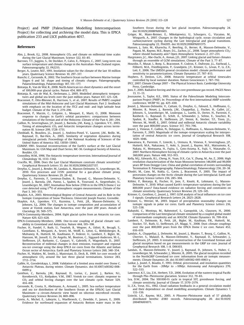
V. Masson-Delmotte et al. / Quaternary Science Reviews 29 (2010) 113–128 127

Project) and PMIP (Paleoclimate Modelling IntercomparisonProject) for collecting and archiving the model data. This is EPICApublication 233 and LSCE publication 4017.

References

Ahn, J., Brook, E.J., 2008. Atmospheric CO2 and climate on millennial time scalesduring the Last Glacial Maximum. Science 322, 83–85.

Barrows, T.T., Juggins, S., De Deckker, P., Calvo, E., Pelejero, C., 2007. Long-term seasurface temperature and climate change in the Australian–New Zealand region.Paleoceanography 22, PA2215.

Berger, A., Loutre, M.F., 1991. Insolation values for the climate of the last 10 millionyears. Quaternary Science Reviews 10, 297–317.

Bianchi, C., Gersonde, R., 2002. The Southern Ocean surface between Marine IsotopeStages 6 and 5d: shape and timing of climatic changes. Palaeogeography,Palaeoclimatology, Palaeoecology 187, 151–177.

Bintanja, R., Van de Wal, R., 2008. North American ice-sheet dynamics and the onsetof 100,000-year glacial cycles. Nature 454, 869–872.

Bintanja, R., van de Wal, R., Oerlemans, J., 2005. Modelled atmospheric tempera-tures and global sea levels over the past million years. Nature 437, 125–128.

Braconnot, P., Otto-Bliesner, B., Harrison, S., et al., 2007. Results of PMIP2 coupledsimulations of the Mid-Holocene and Last Glacial Maximum. Part 2: feedbackswith emphasis on the location of the ITCZ and mid- and high latitude heatbudget. Climate of the Past 3, 279–296.

Braconnot, P., Marzin, C., Gregoire, L., Mosquet, E., Marti, O., 2008. Monsoonresponse to changes in Earth’s orbital parameters: comparisons betweensimulations of the Eemian and of the Holocene. Climate of the Past 4, 281–294.

Caillon, N., Severinghaus, J.P., Jouzel, J., Barnola, J.M., Kang, J., Lipenkov, V.Y., 2003.Timing of atmospheric CO2 and Antarctic temperature changes across termi-nation III. Science 299, 1728–1731.

Cheddadi, R., Beaulieu, J.L., Jouzel, J., Andrieu-Ponel, V., Laurent, J.M., Reille, M.,Raynaud, D., Bar-Hen, A., 2005. Similarity of vegetation dynamics duringinterglacial periods. Proceedings of the National Academy of Sciences of theUnited States of America 102, 13030–13043.

CLIMAP, 1981. Seasonal reconstructions of the Earth’s surface at the Last GlacialMaximum. In: GSA Map and Chart Series, MC-36. Geological Society of America,Boulder, CO.

Connolley, W.M., 1996. The Antarctic temperature inversion. International Journal ofClimatology 16, 1333–1342.

Crucifix, M., 2006. Does the Last Glacial Maximum constrain climate sensitivity?Geophysical Research Letters 33. doi:10.1029/2006GL027137.

Dreyfus, G., Jouzel, J., Bender, M., Landais, A., Masson-Delmotte, V., Leuenberger, M.,2010. Firn processes and d15N: potential for a gas-phase climate proxy.Quarternary Science Reviews 29, 28–42.

Dreyfus, G., Parrenin, F., Lemieux-Dudon, B., Durand, G., Masson-Delmotte, V.,Jouzel, J., Barnola, J.M., Panno, L., Spahni, R., Tisserand, A., Siegenthaler, U.,Leuenberger, M., 2007. Anomalous flow below 2700 m in the EPICA Dome C icecore detected using d18O of atmospheric oxygen measurements. Climate of thePast 3, 341–353.

Ekaykin, A.A., 2003. Meteorological Regime of Central Antarctic and its Role in theIsotopic Composition of Snow Thickness. Universite Joseph Fourier, Grenoble.

Ekaykin, A.A., Lipenkov, V.Y., Kuzmina, I., Petit, J.R., Masson-Delmotte, V.,Johnsen, S.J., 2004. The changes in isotope composition and accumulation ofsnow at Vostok station, East Antarctica, over the past 200 years. Annals ofGlaciology 39, 569–575.

EPICA-Community-Members, 2004. Eight glacial cycles from an Antarctic ice core.Nature 429, 623–628.

EPICA-Community-Members, 2006. One-to-one coupling of glacial climate vari-ability in Greenland and Antarctica. Nature 444, 195–198.

Fischer, H., Fundel, F., Ruth, U., Twarloh, B., Wegner, A., Udisti, R., Becagli, S.,Castellano, E., Morganti, A., Severi, M., Wolff, E., Littot, G., Rothlisberger, R.,Mulvaney, R., Hutterli, M., Kaufmann, P., Federer, U., Lambert, F., Bigler, M.,Hansson, M., Jonsell, U., De Angelis, M., Boutron, C., Siggaard-Andersen, M.-L.,Steffensen, J.P., Barbante, C., Gaspari, V., Gabrielli, P., Wagenbach, D., 2007.Reconstruction of millenial changes in dust emission, transport and regionalsea-ice coverage using the deep EPICA ice cores from the Atlantic and IndianOcean sector of Antarctica. Earth and Planetary Science Letters 260, 340–354.

Fischer, H., Wahlen, M., Smith, J., Mastroiani, D., Deck, B., 1999. Ice core records ofatmospheric CO2 around the last three glacial terminations. Science 283,1712–1714.

Gallee, H., Gorodetskaya, I., 2008. Validation of a limited area model over Dome C,Antarctic Plateau, during winter. Climate Dynamics. doi:10.1007/s00382-008-0499-y.

Genthon, C., Barnola, J.M., Raynaud, D., Lorius, C., Jouzel, J., Barkov, N.I.,Korotkevich, Y.S., Kotlyakov, V.M., 1987. Vostok ice core: climatic response toCO2 and orbital forcing changes over the last climatic cycle. Nature 329,414–418.

Gersonde, R., Crosta, X., Abelmann, A., Armand, L., 2005. Sea-surface temperatureand sea ice distribution of the Southern Ocean at the EPILOG Last GlacialMaximumda circum-Antarctic view based on siliceous microfossil records.Quaternary Science Reviews 24, 869–896.

Govin, A., Michel, E., Labeyrie, L., Waelbroeck, C., Dewilde, F., Jansen, E., 2009.Evidence for northward expansion of Antarctic Bottom water mass in the

Southern Ocean during the last glacial inception. Paleoceanography 24.doi:10.1029/2008PA001603.

Groger, M., Maier-Reimer, E., Mikolajewicz, U., Schurgers, G., Vizcaino, M.,Wingurth, A., 2007. Changes in the hydrological cycle, ocean circulation andcarbon/nutrient cycling during the Last Interglacial and glacial transitions.Paleoceanography 22, PA4205. doi:10.1029/2006PA001375.

Hansen, J., Sato, M., Kharecha, P., Beerling, D., Berner, R., Masson-Delmotte, V.,Pagani, M., Raymo, M.E., Royer, D.L., Zachos, J.C., 2008. Target atmospheric CO2:where should humanity aim? Open Atmospheric Sciences 2, 217–231.

Hargreaves, J.C., Abe-Ouchi, A., Annan, J.D., 2007. Linking glacial and future climatesthrough an ensemble of GCM simulations. Climate of the Past 3, 77–87.

Hourdin, F., Musat, I., Bony, S., Braconnot, P., Codron, F., Dufresne, J.L., Fairhead, L.,Filiberti, M.A., Friedlingstein, P., Grandpeix, J.Y., Krinner, G., Levan, P., Li, Z.X.,Lott, F., 2006. The LMDZ4 general circulation model: climate performance andsensitivity to parameterizations. Climate Dynamics 27, 787–813.

Huybers, P., Denton, G.H., 2008. Antarctic temperature at orbital timescalescontrolled by local summer duration. Nature Geosciences 1, 787–792.

IPCC, 2007. Climate Change 2007 – The Physical Science Basis. Cambridge UniversityPress, Cambridge.

Joos, F., 2005. Radiative forcing and the ice core greenhouse gas record. PAGES News13, 11–13.

Joussaume, S., Taylor, K.E., 1995. Status of the Paleoclimate Modeling Intercom-parison Project (PMIP). In: Proceedings of the first international AMIP scientificconference, WCRP 92, pp. 425–430.

Jouzel, J., Masson-Delmotte, V., Cattani, O., Dreyfus, G., Falourd, S., Hoffmann, G.,Minster, B., Nouet, J., Barnola, J.M., Chappellaz, J., Fischer, H., Gallet, J.C.,Johnsen, S., Leuenberger, M., Loulergue, L., Luethi, D., Oerter, H., Parrenin, F.,Raisbeck, G., Raynaud, D., Schilt, A., Schwander, J., Selmo, E., Souchez, R.,Spahni, R., Stauffer, B., Steffensen, J.P., Stenni, B., Stocker, T.F., Tison, J.L.,Werner, M., Wolff, E., 2007. Orbital and millenial Antarctic climate variabilityover the past 800,000 years. Science 317, 793–796.

Jouzel, J., Vimeux, F., Caillon, N., Delaygue, G., Hoffmann, G., Masson-Delmotte, V.,Parrenin, F., 2003. Magnitude of the isotope–temperature scaling for interpre-tation of central Antarctic ice cores. Journal of Geophysical Research 108,1029–1046.

Kawamura, K., Parrenin, F., Lisiecki, L., Uemura, R., Vimeux, F., Severinghaus, J.P.,Hutterli, M.A., Nakazawa, T., Aoki, S., Jouzel, J., Raymo, M.E., Matsumoto, K.,Nakata, H., Motoyama, H., Fujita, S., Goto-Azuma, K., Fujii, Y., Watanabe, O.,2007. Northern Hemisphere forcing of climatic cycles in Antarctica over the past360,000 years. Nature 448, 912–915.

Kelly, M.J., Edwards, R.L., Cheng, H., Yuan, D.X., Cai, Y., Zhang, M., An, Z., 2006. Highresolution characterization of the Asian Monsoon between 146,000 and 99,000years BP from Dongge Cave, China and global correlation of events surroundingTermination II. Palaeogeography, Palaeoclimatology, Palaeoecology 236, 20–38.

Khodri, M., Cane, M., Kukla, G., Gavin, J., Braconnot, P., 2005. The impact ofprecession changes on the Arctic climate during the Last Interglacial. Earth andPlanetary Science Letters 236, 285–304.

Kohler, P., Bintanja, R., Fischer, H., Joos, F., Knutti, R., Lohmann, G., Masson-Delmotte, V., 2010. What caused Earth’s temperature variations during the last800,000 years? Data-based evidence on radiative forcing and constraints onclimate sensitivity. Quaternary Science Reviews 29, 129–145.

Krinner, G., Genthon, C., Jouzel, J., 1997. GCM analysis of local influences on ice cored signals. Geophysical Research Letters 24, 2825–2828.

Krinner, G., Werner, M., 2003. Impact of precipitation seasonality changes onisotopic signals in polar ice cores. Earth and Planetery Science Letters 216,525–538.

Kubatzki, C., Montoya, M., Rahmstorf, S., Ganopolsk, i.A., Claussen, H., 2000.Comparison of the Last Interglacial climate simulated by a coupled global modelof intermediate complexity and an AOGCM. Climate Dynamics 16, 799–814.

Lambert, F., Delmonte, B., Petit, J.R., Bigler, M., Kaufman, P.R., Hutterli, M.,Stocker, T.F., Ruth, U., Steffensen, J.P., Maggi, V., 2008. Dust–climate couplingsover the past 800,000 years from the EPICA Dome C ice core. Nature 452,616–619.

Landais, A., Chappellaz, J., Delmotte, M., Jouzel, J., Blunier, T., Bourg, C., Caillon, N.,Cherrier, S., Malaize, B., Masson-Delmotte, V., Raynaud, D., Schwander, J.,Steffensen, J.P., 2003. A tentative reconstruction of the Greenland Eemian andglacial inception based on gas measurements in the GRIP ice core. Journal ofGeophysical Research 108, 1–8. D06103.

Landais, A., Masson-Delmotte, V., Jouzel, J., Raynaud, D., Johnsen, S., Huber, C.,Leuenberger, M., Schwander, J., Minster, B., 2005. The glacial inception recordedin the NorthGRIP Greenland ice core: information from air isotopic measure-ments. Climate Dynamics 26. doi:10.1007/s00382-005-0063-y.

Laskar, J., Joutel, F., Boudin, F., 1993. Orbital, precessional, and insolation quantitiesfor the Earth from �20Myr to þ10Myr. Astronomy and Astrophysics 270,522–533.

Lawrence, K.T., Liu, Z.H., Herbert, T.D., 2006. Evolution of the eastern tropical Pacificthrough Plio–Pleistocene glaciation. Science 312, 79–83.

Lea, D.W., 2004. The 100 000-Yr cycle in tropical SST, greenhouse forcing, andclimate sensitivity. Journal of Climate 17, 2170–2179.

Li, Z.X., Treut, H.L., 1992. Cloud radiation feedbacks in a general circulation modeland their dependence on cloud modelling assumptions. Climate Dynamics 7,133–139.

Lisiecki, L.E., Raymo, M.E., 2005. A Pliocene–Pleistocene stack of 57 globallydistributed benthic d18O records. Paleoceanography 20. doi:10.1029/2004PA001071.

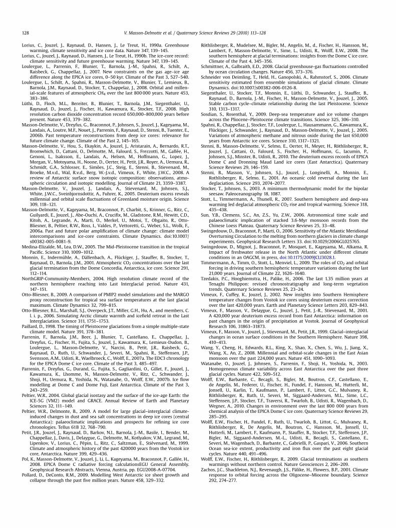
V. Masson-Delmotte et al. / Quaternary Science Reviews 29 (2010) 113–128128

Lorius, C., Jouzel, J., Raynaud, D., Hansen, J., Le Treut, H., 1990a. Greenhousewarming, climate sensitivity and ice core data. Nature 347, 139–145.

Lorius, C., Jouzel, J., Raynaud, D., Hansen, J., Le Treut, H., 1990b. The ice-core record:climate sensitivity and future greenhouse warming. Nature 347, 139–145.

Loulergue, L., Parrenin, F., Blunier, T., Barnola, J.-M., Spahni, R., Schilt, A.,Raisbeck, G., Chappellaz, J., 2007. New constraints on the gas age–ice agedifference along the EPICA ice cores, 0–50 kyr. Climate of the Past 3, 527–540.

Loulergue, L., Schilt, A., Spahni, R., Masson-Delmotte, V., Blunier, T., Lemieux, B.,Barnola, J.M., Raynaud, D., Stocker, T., Chappelaz, J., 2008. Orbital and millen-ial-scale features of atmospheric CH4 over the last 800 000 years. Nature 453,383–386.

Luthi, D., Floch, M.L., Bereiter, B., Blunier, T., Barnola, J.M., Siegenthaler, U.,Raynaud, D., Jouzel, J., Fischer, H., Kawamura, K., Stocker, T.F., 2008. Highresolution carbon dioxide concentration record 650,000–800,000 years beforepresent. Nature 453, 379–382.

Masson-Delmotte, V., Dreyfus, G., Braconnot, P., Johnsen, S., Jouzel, J., Kageyama, M.,Landais, A., Loutre, M.F., Nouet, J., Parrenin, F., Raynaud, D., Stenni, B., Tuenter, E.,2006b. Past temperature reconstructions from deep ice cores: relevance forfuture climate change. Climate of the Past 2, 145–165.

Masson-Delmotte, V., Hou, S., Ekaykin, A., Jouzel, J., Aristarain, A., Bernardo, R.T.,Bromwhich, D., Cattani, O., Delmotte, M., Falourd, S., Frezzotti, M., Gallee, H.,Genoni, L., Isaksson, E., Landais, A., Helsen, M., Hoffmann, G., Lopez, J.,Morgan, V., Motoyama, H., Noone, D., Oerter, H., Petit, J.R., Royer, A., Uemura, R.,Schmidt, G.A., Schlosser, E., Simoes, J.C., Steig, E., Stenni, B., Stievenard, M.,Broeke, M.v.d., Wal, R.v.d., Berg, W.-J.v.d., Vimeux, F., White, J.W.C., 2008. Areview of Antarctic surface snow isotopic composition: observations, atmo-spheric circulation and isotopic modelling. Journal of Climate 21, 3359–3387.

Masson-Delmotte, V., Jouzel, J., Landais, A., Stievenard, M., Johnsen, S.J.,White, J.W.C., Sveinbjornsdottir, A., Fuhrer, K., 2005. Deuterium excess revealsmillennial and orbital scale fluctuations of Greenland moisture origin. Science309, 118–121.

Masson-Delmotte, V., Kageyama, M., Braconnot, P., Charbit, S., Krinner, G., Ritz, C.,Guilyardi, E., Jouzel, J., Abe-Ouchi, A., Crucifix, M., Gladstone, R.M., Hewitt, C.D.,Kitoh, A., Legrande, A., Marti, O., Merkel, U., Motoi, T., Ohgaito, R., Otto-Bliesner, B., Peltier, R.W., Ross, I., Valdes, P., Vettoretti, G., Weber, S.L., Wolk, F.,2006a. Past and future polar amplification of climate change: climate modelintercomparisons and ice-core constraints. Climate Dynamics. doi:10.1007/s00382-005-0081-9.

Medina-Elizalde, M., Lea, D.W., 2005. The Mid-Pleistocene transition in the tropicalPacific. Science 310, 1009–1012.

Monnin, E., Indermuhle, A., Dallenbach, A., Fluckiger, J., Stauffer, B., Stocker, T.,Raynaud, D., Barnola, J.M., 2001. Atmospheric CO2 concentrations over the lastglacial termination from the Dome Concordia, Antarctica, ice core. Science 291,112–114.

NorthGRIP-Community-Members, 2004. High resolution climate record of thenorthern hemisphere reaching into Last Interglacial period. Nature 431,147–151.

Otto-Bliesner, B., 2009. A comparison of PMIP2 model simulations and the MARGOproxy reconstruction for tropical sea surface temperatures at the last glacialmaximum. Climate Dynamics 32, 799–815.

Otto-Bliesner, B.L., Marshall, S.J., Overpeck, J.T., Miller, G.H., Hu, A., and members, C.l. i. p., 2006. Simulating Arctic climate warmth and icefield retreat in the LastInterglaciation. Science 311, 1751–1753.

Paillard, D., 1998. The timing of Pleistocene glaciations from a simple multiple-stateclimate model. Nature 391, 378–381.

Parrenin, F., Barnola, J.M., Beer, J., Blunier, T., Castellano, E., Chappellaz, J.,Dreyfus, G., Fischer, H., Fujita, S., Jouzel, J., Kawamura, K., Lemieux-Dudon, B.,Loulergue, L., Masson-Delmotte, V., Narcisi, B., Petit, J.R., Raisbeck, G.,Raynaud, D., Ruth, U., Schwander, J., Severi, M., Spahni, R., Steffensen, J.P.,Svensson, A.M., Udisti, R., Waelbroeck, C., Wolff, E., 2007a. The EDC3 chronologyfor the EPICA Dome C ice core. Climate of the Past 3, 485–497.

Parrenin, F., Dreyfus, G., Durand, G., Fujita, S., Gagliardini, O., Gillet, F., Jouzel, J.,Kawamura, K., Lhomme, N., Masson-Delmotte, V., Ritz, C., Schwander, J.,Shoji, H., Uemura, R., Yoshida, N., Watanabe, O., Wolff, E.W., 2007b. Ice flowmodelling at Dome C and Dome Fuji, East Antarctica. Climate of the Past 3,243–259.

Peltier, W.R., 2004. Global glacial isostasy and the surface of the ice-age Earth: theICE-5G (VM2) model and GRACE. Annual Review of Earth and PlanetarySciences 32, 111–149.

Peltier, W.R., Delmonte, B., 2009. A model for large glacial–interglacial climate-induced changes in dust and sea salt concentrations in deep ice cores (centralAntarctica): palaeoclimatic implications and prospects for refining ice corechronologies. Tellus 61B 32, 768–790.

Petit, J.R., Jouzel, J., Raynaud, D., Barkov, N.I., Barnola, J.-M., Basile, I., Bender, M.,Chappellaz, J., Davis, J., Delaygue, G., Delmotte, M., Kotlyakov, V.M., Legrand, M.,Lipenkov, V., Lorius, C., Pepin, L., Ritz, C., Saltzman, E., Stievenard, M., 1999.Climate and atmospheric history of the past 420000 years from the Vostok icecore, Antarctica. Nature 399, 429–436.

Pol, K., Masson-Delmotte, V., Jouzel, J., Li, L., Kageyama, M., Braconnot, P., Gallee, H.,2008. EPICA Dome C radiative forcing calculationsEGU General Assembly.Geophysical Research Abstracts, Vienna, Austria, pp. EGU2008-A-07704.

Pollard, D., DeConto, R.M., 2009. Modelling West Antarctic ice sheet growth andcollapse through the past five million years. Nature 458, 329–332.

Rothlisberger, R., Mudelsee, M., Bigler, M., Angelis, M., d., Fischer, H., Hansson, M.,Lambert, F., Masson-Delmotte, V., Sime, L., Udisti, R., Wolff, E.W., 2008. Thesouthern hemisphere at glacial terminations: insights from the Dome C ice core.Climate of the Past 4, 345–356.

Schmittner, A., Galbraith, E.D., 2008. Glacial greenhouse-gas fluctuations controlledby ocean circulation changes. Nature 456, 373–376.

Schneider von Deimling, T., Held, H., Ganopolski, A., Rahmstorf, S., 2006. Climatesensitivity estimated from ensemble simulations of glacial climate. ClimateDynamics. doi:10.1007/s00382-006-0126-8.

Siegenthaler, U., Stocker, T.F., Monnin, E., Luthi, D., Schwander, J., Stauffer, B.,Raynaud, D., Barnola, J.-M., Fischer, H., Masson-Delmotte, V., Jouzel, J., 2005.Stable carbon cycle–climate relationship during the last Pleistocene. Science310, 1313–1317.

Sosdian, S., Rosenthal, Y., 2009. Deep-sea temperature and ice volume changesacross the Pliocene–Pleistocene climate transitions. Science 325, 306–310.

Spahni, R., Chappellaz, J., Stocker, T.F., Loulergue, L., Hausammann, G., Kawamura, K.,Fluckiger, J., Schwander, J., Raynaud, D., Masson-Delmotte, V., Jouzel, J., 2005.Variations of atmospheric methane and nitrous oxide during the last 650,000years from Antarctic ice cores. Science 310, 1317–1321.

Stenni, B., Masson-Delmotte, V., Selmo, E., Oerter, H., Meyer, H., Rothlisberger, R.,Jouzel, J., Cattani, O., Falourd, S., Fischer, H., Hoffmann, G., Iacumin, P.,Johnsen, S.J., Minster, B., Udisti, R., 2010. The deuterium excess records of EPICADome C and Dronning Maud Land ice cores (East Antarctica). QuaternaryScience Reviews 29, 146–159.

Stenni, B., Masson, V., Johnsen, S.J., Jouzel, J., Longinelli, A., Monnin, E.,Rothlisberger, R., Selmo, E., 2001. An oceanic cold reversal during the lastdeglaciation. Science 293, 2074–2077.

Stocker, T., Johnsen, S., 2003. A minimum thermodynamic model for the bipolarseesaw. Paleoceanography 18, 1087.

Stott, L., Timmermann, A., Thunell, R., 2007. Southern hemisphere and deep-seawarming led deglacial atmospheric CO2 rise and tropical warming. Science 318,435–438.

Sun, Y.B., Clemens, S.C., An, Z.S., Yu, Z.W., 2006. Astronomical time scale andpalaeoclimatic implication of stacked 3.6-Myr monsoon records from theChinese Loess Plateau. Quaternary Science Reviews 25, 33–48.

Swingedouw, D., Braconnot, P., Marti, O., 2006. Sensitivity of the Atlantic MeridionalOverturning Circulation to the melting from northern glaciers in climate changeexperiments. Geophysical Research Letters 33. doi:10.1029/2006GL025765.

Swingedouw, D., Mignot, J., Braconnot, P., Mosquet, E., Kageyama, M., Alkama, R.Impact of freshwater release in the North Atlantic under different climateconditions in an OAGCM, in press, doi:10.1175/2009JCLI3028.1.

Timmermann, A., Timm, O., Stott, L., Menviel, L., 2009. The roles of CO2 and orbitalforcing in driving southern hemispheric temperature variations during the last21,000 years. Journal of Climate 22, 1626–1640.

Tzedakis, P.C., Hooghiemstra, H., Palike, H., 2006. The last 1.35 million years atTenaghi Philippon: revised chronostratigraphy and long-term vegetationtrends. Quaternary Science Reviews 25, 23–24.

Vimeux, F., Cuffey, K., Jouzel, J., 2002. New insights into Southern Hemispheretemperature changes from Vostok ice cores using deuterium excess correctionover the last 420,000 years. Earth and Planetary Science Letters 203, 829–843.

Vimeux, F., Masson, V., Delaygue, G., Jouzel, J., Petit, J.-R., Stievenard, M., 2001.A 420,000 year deuterium excess record from East Antarctica: information onpast changes in the origin of precipitation at Vostok. Journal of GeophysicalResearch 106, 31863–31873.

Vimeux, F., Masson, V., Jouzel, J., Stievenard, M., Petit, J.R., 1999. Glacial–interglacialchanges in ocean surface conditions in the Southern Hemisphere. Nature 398,410–413.

Wang, Y., Cheng, H., Edwards, R.L., King, X., Shao, X., Chen, S., Wu, J., Jiang, X.,Wang, X., An, Z., 2008. Millennial and orbital-scale changes in the East Asianmonsoon over the past 224,000 years. Nature 451, 1090–1093.

Watanabe, O., Jouzel, J., Johnsen, S., Parrenin, F., Shoji, H., Yoshida, N., 2003.Homogeneous climate variability across East Antarctica over the past threeglacial cycles. Nature 422, 509–512.

Wolff, E.W., Barbante, C., Becagli, S., Bigler, M., Boutron, C.F., Castellano, E.,de Angelis, M., Federer, U., Fischer, H., Fundel, F., Hansson, M., Hutterli, M.,Jonsell, U., Karlin, T., Kaufmann, P., Lambert, F., Littot, G.C., Mulvaney, R.,Rothlisberger, R., Ruth, U., Severi, M., Siggaard-Andersen, M.L., Sime, L.C.,Steffensen, J.P., Stocker, T.F., Traversi, R., Twarloh, B., Udisti, R., Wagenbach, D.,Wegner, A., 2010. Changes in environment over the last 800 000 years fromchemical analysis of the EPICA Dome C ice core. Quaternary Science Reviews 29,285–295.

Wolff, E.W., Fischer, H., Fundel, F., Ruth, U., Twarloh, B., Littot, G., Mulvaney, R.,Rothlisberger, R., De Angelis, M., Boutron, C., Hansson, M., Jonsell, U.,Hutterli, M., Lambert, F., Kaufmann, P., Stauffer, B., Stocker, T.F., Steffensen, J.P.,Bigler, M., Siggaard-Andersen, M.-L., Udisti, R., Becagli, S., Castellano, E.,Severi, M., Wagenbach, D., Barbante, C., Gabrielli, P., Gaspari, V., 2006. SouthernOcean sea-ice extent, productivity and iron flux over the past eight glacialcycles. Nature 440, 491–496.

Wolff, E.W., Fischer, H., Rothlisberger, R., 2009. Glacial terminations as southernwarmings without northern control. Nature Geosciences 2, 206–209.

Zachos, J.C., Shackleton, N.J., Revenaugh, J.S., Palike, H., Flowers, B.P., 2001. Climateresponse to orbital forcing across the Oligocene–Miocene boundary. Science292, 274–277.