Embed Size (px)
Citation preview

Nothing is mightier than an ideawhose time has come.
V. M. Hugo (1802-1885)
12Quantum Electrodynamics
In Chapter 7 we have learned how to quantize relativistic free fields and in Chap-ters 10 and 11 how to deal with interactions if the coupling is small. So far, this wasonly done perturbatively. Fortunately, there is a large set of physical phenomenafor which perturbative techniques are sufficient to supply theoretical results thatagree with experiment. In particular, there exists one theory, where the agreementis extremely good. This is the quantized theory of interacting electrons and photonscalled quantum electrodynamics, or shortly QED.
12.1 Gauge Invariant Interacting Theory
The free Lagrangians of electrons and photons are known from Chapter 5 as
L(x) =e
L(x) +γ
L(x), (12.1)
with
e
L(x) = ψ(x) (i/∂ −m)ψ(x), (12.2)γ
L(x) = −1
4Fµν(x)F
µν(x) = −1
4[∂µAν(x)− ∂νAµ(x)] [∂
µAν(x)− ∂νAµ(x)] .(12.3)
When quantizing the photon field, there were subtleties due to the gauge freedomin the choice of the gauge fields Aµ:
Aµ(x) → Aµ(x) + ∂µΛ(x). (12.4)
For this reason, there were different ways of constructing a Hilbert space of freeparticles. The first, described in Subsection 7.5.1, was based on the quantizationof only the two physical transverse degrees of freedom. The time component ofthe gauge field A0 and the spatial divergence ∇ ·A(x) had no canonically conjugatefield and were therefore classical fields, with no operator representation in the Hilbertspace. The two fields are related by Coulomb’s law which reads, in the absence ofcharges:
∇2A0(x) = −∂0∇ ·A(x). (12.5)
801

802 12 Quantum Electrodynamics
Only the transverse components, defined by
Ai⊥(x) ≡(
δij −∇i∇j/∇2)
Aj(x, t), (12.6)
were operators. These components represent the proper dynamical variables of thesystem. After fulfilling the canonical commutation rules, the positive- and negative-frequency parts of these fields define creation and annihilation operators for theelectromagnetic quanta. These are the photons of right and left circular polarization.
This method had an esthetical disadvantage that two of the four components ofthe vector field Aµ(x) require a different treatment. The components which becomeoperators change with the frame of reference in which the canonical quantizationprocedure is performed.
To circumvent this, a covariant quantization procedure was developed by Guptaand Bleuler in Subsection 7.5.3. In their quantization scheme, the propagator took apleasant covariant form. But this happened at the expense of another disadvantage,that this Lagrangian describes the propagation of four particles of which only twocorrespond to physical states. Accordingly, the Hilbert space contained two kindsof unphysical particle states, those with negative and those with zero norm. Still,a physical interpretation of this formalism was found with the help of a subsidiarycondition that selects the physical subspace in the Hilbert space of free particles.
The final and most satisfactory successful quantization was developed by Faddeevand Popov [1] and was described in Subsection 7.5.2. It started out by modifyingthe initial photon Lagrangian by a gauge-fixing term
LGF(x) = −D∂µAµ(x) + αD2(x)/2. (12.7)
After that, the quantization can be performed in the usual canonical way.
12.1.1 Reminder of Classical Electrodynamics of Point Particles
In this chapter we want to couple electrons and photons with each other by anappropriate interaction and study the resulting interacting field theory, the famousquantum electrodynamics (QED). Since the coupling should not change the twophysical degrees of freedom described by the four-component photon field Aµ, it isimportant to preserve the gauge invariance, which was so essential in assuring thecorrect Hilbert space of free photons. The prescription how this can be done has beenknown for a long time in the context of classical electrodynamics of point particles.In that theory, a free relativistic particle moving along an arbitrarily parametrizedpath xµ(τ) in four-space is described by an action
A = −mc2∫
dτ
√
dxµ
dτ
dxµdτ
= −mc2∫
dt
[
1− v2(t)
c2
]1/2
, (12.8)
where x0(τ) = t is the time and dx/dt = v(t) the velocity along the path. If theparticle has a charge e and lies at rest at position x, its potential energy is
V (t) = eφ(x, t), (12.9)

12.1 Gauge Invariant Interacting Theory 803
where
φ(x, t) = A0(x, t). (12.10)
In our convention, the charge of the electron e has a negative value to agree withthe sign in the historic form of the Maxwell equations
∇ · E(x) = −∇2φ(x) = ρ(x),
∇×B(x)− E(x) = ∇×∇×A(x)− E(x)
= −[
∇2A(x)−∇ ·∇A(x)
]
− E(x) =1
cj(x). (12.11)
If the electron moves along a trajectory x(t), the potential energy becomes
V (t) = eφ (x(t), t) . (12.12)
In the Lagrangian L = T − V , this contributes with the opposite sign
Lint(t) = −eA0 (x(t), t) , (12.13)
adding a potential term to the interaction
Aint|pot = −e∫
dtA0 (x(t), t) . (12.14)
Since the time t coincides with x0(t)/c of the trajectory, this can be expressed as
Aint|pot = −ec
∫
dx0A0(x). (12.15)
In this form it is now quite simple to write down the complete electromagneticinteraction purely on the basis of relativistic invariance. The minimal Lorentz-invariant extension of (12.15) is obviously
Aint = −ec
∫
dxµAµ(x). (12.16)
Thus, the full action of a point particle can be written, more explicitly, as
A =∫
dtL(t) = −mc∫
ds− e
c
∫
dxµAµ(x)
= −mc2∫
dt
[
1− v2
c2
]1/2
− e∫
dt(
A0 − 1
cv ·A
)
. (12.17)
The canonical formalism supplies the canonically conjugate momentum
P =∂L
∂v= m
v√
1− v2/c2+e
cA ≡ p+
e
cA. (12.18)

804 12 Quantum Electrodynamics
Thus the velocity is related to the canonical momentum and external vector potentialvia
v
c=
P− ecA
√
(
P− ecA)2
+m2c2. (12.19)
This can be used to calculate the Hamiltonian as the Legendre transform
H =∂L
∂vv − L = P · v − L, (12.20)
with the result
H = c
√
(
P− e
cA
)2
+m2c2 + eA0. (12.21)
At nonrelativistic velocities, this has the expansion
H = mc2 +1
2m
(
P− e
cA
)2
+ eA0 + . . . . (12.22)
The rest energy mc2 is usually omitted in this limit.
12.1.2 Electrodynamics and Quantum Mechanics
When going over from quantum mechanics to second-quantized field theory in Chap-ter 2, we found the rule that a nonrelativistic Hamiltonian
H =p2
2m+ V (x) (12.23)
becomes an operator
H =∫
d3xψ†(x, t)
[
−∇2
2m+ V (x)
]
ψ(x, t). (12.24)
For brevity, we have omitted a hat on top of H and the fields ψ†(x, t), ψ(x, t).Following the rules of Chapter 2, we see that the second-quantized form of theinteracting nonrelativistic Hamiltonian in a static A(x) field with the Hamiltonian(12.22) (minus mc2),
H =(P− eA)2
2m+ eA0, (12.25)
is given by
H =∫
d3xψ†(x, t)
[
− 1
2m
(
∇− ie
cA
)2
+ eA0
]
ψ(x, t). (12.26)
12.1 Gauge Invariant Interacting Theory 805
The action of this theory reads
A =∫
dtL =∫
dt∫
d3x[
ψ†(x, t)(
i∂t + eA0)
ψ(x, t)
+1
2mψ†(x, t)
(
∇− ie
cA
)2
ψ(x, t)]
. (12.27)
It is easy to verify that (12.26) reemerges from the Legendre transform
H =∂L
∂ψ(x, t)ψ(x, t)− L. (12.28)
The action (12.27) holds also for time-dependent Aµ(x)-fields.These equations show that electromagnetism is introduced into a free quantum
theory of charged particles following the minimal substitution rule
∇ → ∇− ie
cA(x, t),
∂t → ∂t + ieA0(x, t), (12.29)
or covariantly:
∂µ → ∂µ − ie
cAµ(x). (12.30)
The substituted action has the important property that the gauge invariance ofthe free photon action is preserved by the interacting theory: If we perform thegauge transformation
Aµ(x) → Aµ(x) + ∂µΛ(x), (12.31)
i.e.,
A0(x, t) → A0(x, t) + ∂tΛ(x, t),
A(x, t) → A(x, t)−∇Λ(x, t), (12.32)
the action remains invariant provided thet we simultaneously change the fieldsψ(x, t) of the charged particles by a spacetime-dependent phase
ψ (x, t) → e−i(e/c)Λ(x,t)ψ(x, t). (12.33)
Under this transformation, the space and time derivatives of the field change like
∇ψ(x, t) → e−i(e/c)Λ(x,t)[
∇− ie
c∇Λ(x, t)
]
ψ,
∂tψ → e−i(e/c)Λ(x,t) (∂t − ie∂tΛ)ψ(x, t). (12.34)
The covariant derivatives in the action (12.27) have therefore the following simpletransformation law:
(
∇− ie
cA
)
ψ(x, t) → e−i(e/c)Λ(x,t)(
∇− ie
cA
)
ψ(x, t),(
∂t + ie
cA0)
ψ(x, t) → e−i(e/c)Λ(x,t)(
∂t + ieA0)
ψ(x, t). (12.35)

806 12 Quantum Electrodynamics
These combinations of derivatives and gauge fields are called covariant derivatives
and are written as
Dψ(x, t) ≡(
∇− ie
cA
)
ψ(x, t),
Dtψ(x, t) ≡(
∂t + ieA0)
ψ(x, t), (12.36)
or, in four-vector notation, as
Dµψ(x) =(
∂µ + ie
cAµ
)
ψ(x). (12.37)
Here the adjective “covariant” does not refer to the Lorentz group but to the gaugegroup. It records the fact that Dµψ transforms under local gauge changes (12.29)of ψ in the same way as ψ itself in (12.33):
Dµψ(x) → e−i(e/c)Λ(x)Dµψ(x). (12.38)
With the help of such covariant derivatives, any action which is invariant underglobal phase changes by a constant phase angle [i.e., U(1)-invariant in the sensediscussed in Section 8.11.1]
ψ(x) → e−iαψ(x), (12.39)
can easily be made invariant under local gauge transformations (12.31). We merelyhave to replace all derivatives by covariant derivatives (12.37), and add to the fieldLagrangian the gauge-invariant photon expression (12.3).
12.1.3 Principle of Nonholonomic Gauge Invariance
The minimal substitution rule can be viewed as a consequence of a more generalprinciple of nonholonomic gauge invariance. The physics of the initial action (12.17)is trivially invariant under the addition of a term
∆A = −ec
∫
dt xµ(t)∂µΛ(x). (12.40)
The integral runs over the particle path and contributes only a pure surface termfrom the endpoints:
∆A = −ec[Λ(xb)− Λ(xa)] . (12.41)
This does not change the particle trajectories. If we now postulate that the dynam-ical laws of physics remain also valid when we admit multivalued gauge functionsΛ(x) for which the Schwarz integrability criterion is violated, i.e., which possessnoncommuting partial derivatives:
(∂µ∂ν − ∂ν∂µ)Λ(x) 6= 0. (12.42)

12.1 Gauge Invariant Interacting Theory 807
Then the derivatives
Aµ(x) = ∂µΛ(x) (12.43)
have a nonzero curl Fµν = (∂µAν − ∂µAν) = (∂µ∂ν − ∂ν∂µ)Λ(x) 6= 0, and the action(12.41) coincides with the interaction (12.16).
Similarly we can derive the equations of motion of a wave function in an elec-tromagnetic field from that in field-free space by noting the trivial invariance ofquantum mechanics without fields under gauge transformations (12.33), and by ex-tending the set of permissible gauge functions Λ(x) to multivalued functions forwhich the partial derivatives do not commute as in (12.42).
In either case, the nonholonomic gauge transformations convert the physical lawsobeyed by a particle in Euclidean spacetime without electromagnetism into thosewith electromagnetic fields.
This principle is discussed in detail in the literature [11]. It can be generalizedto derive the equations of motion in a curved spacetime from those in flat spacetimeby nonholonomic coordinate transformations which introduce defects in spacetime.
12.1.4 Electrodynamics and Relativistic Quantum Mechanics
Let us follow this rule for relativistic electrons and replace, in the Lagrangian (12.2),the differential operator /∂ = γµ∂µ by
γµ(
∂µ + ie
cAµ
)
=(
/∂ + ie
c/A)
≡ /D . (12.44)
In this way we arrive at the Lagrangian of quantum electrodynamics (QED)
L(x) = ψ(x) (i/D −m)ψ(x)− 1
4F 2µν . (12.45)
The classical field equations can easily be found by extremizing the action withrespect to all fields, which gives
δAδψ(x)
= (i/D −m)ψ(x) = 0, (12.46)
δAδAµ(x)
= ∂νFνµ(x)− 1
cjµ(x) = 0, (12.47)
where jµ(x) is the current density:
jµ(x) ≡ ecψ(x)γµψ(x). (12.48)
Equation (12.47) coincides with the Maxwell equation for the electromagnetic fieldaround a classical four-dimensional vector current jµ(x):
∂νFνµ(x) =
1
cjµ(x). (12.49)

808 12 Quantum Electrodynamics
In the Lorenz gauge ∂µAµ(x) = 0, this equation reduces to
−∂2Aµ(x) = 1
cjµ(x). (12.50)
The current density jµ combines the charge density ρ(x) and the spatial currentdensity j(x) of particles of charge e in a four-vector:
jµ = (cρ, j) . (12.51)
In terms of electric and magnetic fields Ei = F i0, Bi = −F jk, the field equations(12.49) turn into the Maxwell equations
∇ · E = ρ = eψγ0ψ = eψ†ψ, (12.52)
∇×B− E =1
cj =
e
cψ ψ. (12.53)
The first is Coulomb’s law, the second is Ampere’s law in the presence of chargesand currents.
Note that the physical units employed here differ from those used in many booksof classical electrodynamics [12], by the absence of a factor 1/4π on the right-handside. The Lagrangian used in those books is
L(x) = − 1
8πF 2µν(x)−
1
cjµ(x)Aµ(x) (12.54)
=1
4π
[
E2(x)−B2(x)]
−[
ρ(x)φ(x)− 1
cj(x) ·A(x)
]
,
which leads to Maxwell’s field equations
∇ · E = 4πρ,
∇×B− E =4π
cj. (12.55)
The form employed conventionally in quantum field theory arises from this by re-placing A →
√4πA and e → −
√4πe2. The charge of the electron in our units has
therefore the numerical value
e = −√4πα ≈ −
√
4π/137 (12.56)
rather than e = −√α.
12.2 Noether’s Theorem and Gauge Fields
In electrodynamics, the conserved charge resulting from the U(1)-symmetry of thematter Lagrangian by Noether’s theorem (recall Chapter 8) is the source of a mass-less particle, the photon. This is described by a gauge field which is minimallycoupled to the conserved current. A similar structure will be seen in Chapters 27

12.2 Noether’s Theorem and Gauge Fields 809
and 28 to exist for many internal symmetries giving rise to nonabelian versions ofthe photon, for instance the famous W - and Z-vector mesons, which mediate theweak interactions, or the gluons which give rise to strong interactions. It is usefulto recall Noether’s derivation of conservation laws in such theories.
For a a locally gauge invariant theory, the conserved matter current can no longerbe found by the rule (8.118), which was so useful in the globally invariant theory.Indeed, in quantum electrodynamics, the derivative with respect to the local fieldtransformation ǫ(x) would be simply given by
jµ =δL∂∂µΛ
, (12.57)
since this would be identically equal to zero, due to local gauge invariance. We may,however, subject just the matter field to a local gauge transformation at fixed gaugefields. Then we obtain the correct current
jµ ≡ ∂L∂∂µΛ
∣
∣
∣
∣
∣
γ
. (12.58)
Since the complete change under local gauge transformations δxsL vanishes identi-cally, we can alternatively vary only the gauge fields and keep the electron fieldfixed
jµ = − ∂L∂∂µΛ
∣
∣
∣
∣
∣
e
. (12.59)
This is done most simply by forming the functional derivative with respect to the
gauge field, and by omitting the contribution ofγ
L:
jµ = − ∂e
L∂∂µΛ
. (12.60)
An interesting consequence of local gauge invariance can be found for the gaugefield itself. If we form the variation of the pure gauge field action
δsγ
A =∫
d4x tr
δxsAµ
γ
Aǫ
δAµ
, (12.61)
and insert, for δxsA, an infinitesimal pure gauge field configuration
δxsAµ = −i∂µΛ(x), (12.62)
the variation must vanish for all Λ(x). After a partial integration, this implies thelocal conservation law ∂µj
µ(x) = 0 for the current
jµ(x) = −i δγ
AδAµ
. (12.63)

810 12 Quantum Electrodynamics
In contrast to the earlier conservation laws derived for matter fields which were validonly if the matter fields obey the Euler-Lagrange equations, the current conservationlaw for gauge fields is valid for all field configurations. It is an identity , oftencalled Bianchi identity due to its close analogy with certain identities in Riemanniangeometry.
To verify this, we insert the Lagrangian (12.3) into (12.63) and find jν =∂µF
µν/2. This current is trivially conserved for any field configuration due to theantisymmetry of F µν .
12.3 Quantization
The canonical formalism can be used to identify canonical momenta of the fieldsψ(x) and Ai(x):
πψ(x) =∂L
∂ψ(x)= ψ†(x), (12.64)
and
πAi(x) ≡ πi(x) = F 0i(x) = −Ei(x), (12.65)
and to find the Hamiltonian density
H(x) =∂L
∂ψ(x)ψ(x) +
∂L(x)∂Ak(x)
− L(x) (12.66)
= ψ(−i ∇+m)ψ +1
2(E2 +B2) +∇A0 · E+ eψγµψA
µ.
Here, and in all subsequent discussions, we use natural units in which the lightvelocity is equal to unity.
The quantization procedure in the presence of interactions now goes as follows:The Dirac field of the electron has the same equal-time anticommutation rules as inthe free case:
ψa(x, t), ψ†b(x
′, t) = δ(3)(x′ − x)δab,
ψ(x, t), ψ(x′, t) = 0, (12.67)
ψ†(x, t)ψ†(x′t) = 0.
For the photon field we first write down the naive commutation rules of the spatialcomponents:
− [Ei(x, t), Aj(x′, t)] = −iδ(3)(x− x′)δij (12.68)
[Ai(x, t), Aj(x′, t)] = 0, (12.69)
[Ei(x, t), Ej(x′, t)] = 0. (12.70)
12.3 Quantization 811
As in Eq. (7.346), the first commutator cannot be true here, since by Coulomb’slaw (12.52):
∇ · E = −∇ · A−∇2A0
= eψ†ψ, (12.71)
and we want the canonical fields Ai to be independent of ψ, ψ†, and thus to commute
with them. The contradiction can be removed just as in the free case by postulating(12.68) only for the transverse parts of Ei, and using δTij(x−x′) as in (7.347), whileletting the longitudinal part ∇ ·A(x, t) be a c-number field, since it commutes withall Ai(x, t). The correct commutation rules are the following:
[
Aj(x, t), Aj(x′, t)
]
= −iδTij(x− x′),
[Aj(x, t), Aj(x′, t)] = 0, (12.72)
[
Ai(x, t), Aj(x′, t)
]
= 0.
To calculate the temporal behavior of an arbitrary observable composed of ψ, ψ†,and of Ai, Ai fields, only one more set of commutation rules has to be specifiedwhich are those with A0. This field occurs in the Hamiltonian density (12.66) andis not one of the canonical variables. Moreover, in contrast to the free-field case inSection 7.5, it is no longer a c-number. To see this, we express A0 in terms of thedynamical fields using Coulomb’s law (12.71):
A0(x, t) =1
4π
∫
d3x′1
|x′ − x|(
eψ†ψ +∇ · A)
(x′, t). (12.73)
This replaces Eq. (4.268) in the presence of charges. In an infinite volume withasymptotically vanishing fields, there is no freedom of adding a solution of thehomogeneous Poisson equation (4.269). Hence, whereas ∇ ·A is a c-number field,the time component of the gauge field A0 is now a non-local operator involving thefermion fields. Since these are independent of the electromagnetic field, A0 stillcommutes with the canonical Ai, Aj fields:
[
A0(x, t), Ai(x′)]
=[
A0(x, t), Ai(x′, t)]
= 0. (12.74)
The commutator with the Fermi fields, on the other hand, is nonzero:
[
A0(x, t), ψ(x′, t)]
= − e
4π|x− x′|ψ(x, t). (12.75)
Note the peculiar property of A0: It does not commute with the electron field, nomatter how large the distance between the space points is. This property is callednonlocality. It is a typical property of the present transverse covariant quantizationprocedure.
Certainly, the arbitrary c-number function ∇ ·A(x, t) can be made zero by anappropriate gauge transformation, as in (4.257).
812 12 Quantum Electrodynamics
In the Hamiltonian, the field A0 can be completely removed by a partial inte-gration:
∫
d3x∇A0 · E = −∫
d3xA0∇ · E, (12.76)
if we set the surface term equal to zero. Using now the field equation
∇ · E = eψ†ψ, (12.77)
we derive
H =∫
d3xH (12.78)
=∫
d3x
ψ[
−i · (∇− ie
cA) +m
]
ψ +1
2
(
E2 +B2)
.
When looking at this expression, one may wonder where the electrostatic interactionhas gone. The answer is found by decomposing the electric field
Ei = −∂0Ai + ∂iA0 (12.79)
into longitudinal and transverse parts EiL and Ei
T with EL · ET = 0:
EiL = ∂i
(
A0 − ∂i∂i
∇2 A
j
)
,
EiT = −∂0
(
δij − ∂i∂j
∇2
)
Aj . (12.80)
Then the field energy becomes
1
2
∫
d3x(
E2 +B2)
=1
2
∫
d3x(
E2T +B2
)
+1
2
∫
d3xE2L. (12.81)
Using (12.73), we see that the longitudinal field is simply given by
EL(x) = − 1
4π∇
∫
d3x′1
|x− x′|eψ†(x′, t)ψ(x′, t)
= ∇
[
1
∇2 eψ
†(x)ψ(x)]
. (12.82)
It is the Coulomb field caused by the charge density of the electron eψ†(x)ψ(x). Thefield energy carried by Ei
L(x) is
1
2
∫
d3xE2L(x) =
e2
2
∫
d3x
∇
[
1
∇2ψ
†(x)ψ(x)]2
=−e2
2
∫
d3xψ†(x)ψ(x)1
∇2ψ
†(x)ψ(x)
=e2
8π
∫
d3xd3x′ ψ†(x, t)ψ(x, t)1
|x− x′|ψ†(x′, t)ψ(x′, t). (12.83)

12.4 Perturbation Theory 813
This coincides precisely with the classical Coulomb energy associated with the chargedensity (12.52). The term 1
2
∫
d3x (E2T +B2) in Eq. (12.81), on the other hand, is
an operator and contains the energy of the field quanta.In order to develop a perturbation theory for QED in this quantization, we
must specify the free and interacting parts of the action. Since A0 and ∇·A areunquantized and appear only quadratically in the action, they may be eliminatedin the action in the same way as in the energy, so that the action becomes
A =∫
d4x
ψ(x)(i/∂ −M)ψ(x) +1
2
[
E2T (x)−B2(x)
]
+Aint. (12.84)
The first two terms are the actions of the Dirac field ψ and transverse electromagneticfields AT , and Aint denotes the interaction
Aint=− e2
8π
∫
dt∫
d3xd3x′ψ†(x, t)ψ(x, t)1
|x− x′|ψ(x′, t)ψ(x′, t) +
∫
d4x1
cj ·AT .
(12.85)The interaction contains two completely different terms: The first is an instanta-neous Coulomb interaction at a distance, which takes place without retardation andinvolves the charge density. It is a nontrivial field-theoretic exercise to show thatthe absence of retardation in the first term is compensated by current-current inter-action resulting from the second term, so that it does not cause any conflicts withrelativity. This will be done at the end of Section 14.16.
The special role of the Coulomb interaction is avoided from the beginning in theGupta-Bleuler quantization procedure that was discussed in Subsection 7.5.2. Therethe free action was
A =∫
d4x[
ψ (i/∂ −m)ψ − 1
4F µνFµν −D∂µAµ +D2/2
]
, (12.86)
and the interaction had the manifestly covariant form
Aint = −∫
d4x jµAµ. (12.87)
12.4 Perturbation Theory
Let us now set up the rules for building the Feynman diagrams to calculate theeffect of the interaction. In this context, we shall from now on attach, to the freepropagator, a subscript 0. The propagator of the free photon depends on the gauge.It is most simple in the Gupta-Bleuler quantization scheme, where [see (7.510)]
Gµν0 (x, x′) = −gµνG0(x, x
′) = −gµν∫
d4q
(2π)4i
q2 + iηe−ik(x−x
′). (12.88)
Since we want to calculate the effect of interactions, we shall from now on attach tothe free propagator a subscript 0.

814 12 Quantum Electrodynamics
The free-particle propagator of the electrons was given in (7.289):
S0(x− x′) =∫
d4p
(2π)4i
/p −M + iηe−ip(x−x
′). (12.89)
In a Wick expansion of eiAint
, each contraction is represented by one of these twopropagators:
Aµ(x)Aν(x′) = Gµν0 (x− x′), (12.90)
ψ(x)ψ(x′) = S0(x− x′). (12.91)
In the Feynman diagrams, they are pictured by the lines
= −gµν i
q2 + iǫ ,
=i
/p −m.
(12.92)
(12.93)
The interaction Lagrangian
Lint = −eψγµAµ(x) (12.94)
is pictured by the vertex
= −eγµ.(12.95)
With these graphical elements we must form all Feynman diagrams which can con-tribute to a given physical process.
In the transverse quantization scheme, the Feynman diagrams are much morecomplicated. Recalling the propagator (7.361), the photon line stands now for
= P µνphys(q)
i
q2 + iǫ, (12.96)
with the physical off-shell polarization sum [compare (12.7)]
P µνphys(q) = −gµν − qµqν
(qη)2 − q2+ qη
qµην + qνηµ(qη)2 − q2
− ηµηνq2
(qη)2 − q2. (12.97)
The photon propagator is very complicated due to the appearance of the frame-dependent auxiliary vector η = (1, 0, 0, 0). As a further complication, there are

12.4 Perturbation Theory 815
diagrams from the four-fermion Coulomb interactions in (12.85). These can bepictured by a photon exchange diagram
=i
q2γ0 × γ0. (12.98)
They may be derived from an auxiliary interaction
Aint = −∫
d4x j0A0, (12.99)
assuming the A0-field to have the propagator
=i
q20 0 . (12.100)
If this propagator is added to the physical one, it cancels precisely the last term inthe off-shell polarization sum (12.97), which becomes effectively
P µνphys,eff(k) = −gµν − qµqν
(qη)2 − q2+ qη
qµην + qνηµ(qη)2 − q2
. (12.101)
Of course, the final physical results cannot depend on the frame in which thetheory is quantized. Thus it must be possible to drop all η-dependent terms. Weshall now prove this in three steps:
First, a photon may be absorbed (or emitted) by an electron which is on theirmass shell before and after the process. The photon propagator is contracted withan electron current as follows
u(p′, s′3)γµu(p, s′3)P
µνphys,eff(q). q = p′ − p. (12.102)
Since the spinors on the right and left-hand side satisfy the Dirac equation, thecurrent is conserved and satisfies
u(p′, s′3)γµu(p, s′3)q
µ = 0. (12.103)
This condition eliminates the terms containing the vector qµ in the polarization sum(12.101). Only the reduced polarization sum
P µνred(q) = −gµν (12.104)
survives, which is the polarization tensor of the Gupta-Bleuler propagator (12.88).The same cancellation occurs if a photon is absorbed by an internal line, although
due to a slightly more involved mechanism. An internal line may arise in two ways.

816 12 Quantum Electrodynamics
Figure 12.1 An electron on the mass shell absorbing several photons.
An electron may enter a Feynman diagram on the mass shell, absorb a number ofphotons, say n of them, and leave again on the mass shell as shown in Fig. 12.1.The associated off-shell amplitude is
a(p′, p, qi) =1
/p ′ −M/q n
1
/p n−1 −M/q n−1/q n−1 · · · /q 3
1
/p 2 −M/q 2
1
/p 1 −M/q 1. (12.105)
It has to be amputated and evaluated between the initial and final spinors, whichamounts to multiplying it from the left and right with u(p′, s′3)(/p
′ −M) and with(/p−M)u(p, s3), respectively. If an additional photon is absorbed, it must be insertedas shown in Fig. 12.2. At each vertex, there is no current conservation since the
Figure 12.2 An electron on the mass shell absorbing several photons, plus one additional
photon.
photon lines are not on their mass shell. Nevertheless, the sum of all n+2 diagramsdoes have a conserved current.
To prove this we observe the following Ward-Takahashi identity for free particles[2, 3]:
1
/p r + /q −M/q
1
/p r −M=
1
/p r −M− 1
/p r + /q −M. (12.106)
More details on this important identity will be given in the next section.The sum of all off-shell absorption diagrams can be written as
a(p′, p, qi; q) =1
/p ′ + /q −M/q n
1
/p n−1 + /q −M/q n−1 · · ·

12.4 Perturbation Theory 817
· · · 1
/p r + /q −M/q
1
/p r −M· · · /q 2
1
/p 1 −M/q 1u(p, s3), (12.107)
to be evaluated between u(p′ + q, s′3)(/p′ + /q − M) and (/p − M)u(p, s3). With
the help of the Ward-Takahashi identity we can now remove the /q recursively froma(p′, p, qi; q) and remain with the difference
a(p′, p, qi; q) = a(p′, p, qi)− a(p′ + q, p+ q, qi). (12.108)
When evaluating the right-hand side between the above spinors, we see that thefirst term in the difference vanishes since the left-hand spinor satisfies the Diracequation. The same thing holds for the second term and the right-hand spinor.Thus the polarization sum in the photon propagator can again be replaced by thereduced expression (12.104).
Finally, the electron line can be closed to a loop as shown in Fig. 12.3. Here the
Figure 12.3 An internal electron loop absorbing several photons, plus an additional
photon, and leaving again on the mass shell.
amplitude (12.108) appears in a loop integral with an additional photon vertex:
∫
d4p
(2π)4tr[/q a(p′, p, qi; q)] =
∫
d4p
(2π)4tr/q [a(p′, p, qi)− a(p′ + q, p+ q, qi)]. (12.109)
If the divergence of the integral is made finite by a dimensional regularization, theloop integral is translationally invariant in momentum space and the amplitudedifference vanishes. Hence, also in this case, the polarization sum can be replacedby the reduced expression (12.104).
Thus we have shown that due to current conservation and the Ward-Takahashiidentity, the photon propagator in all Feynman diagrams can be replaced by
(12.110)
818 12 Quantum Electrodynamics
= Gµν(q) =−igµνq2 + iη
.
As a matter of fact, for the same reason, any propagator
(12.111)= Gµν(q) = − i
q2
[
gµν −qµqνq2
(1− α)
]
can be used just as well, and the parameter α is arbitrary. Indeed, this is thepropagator arising when adding to the gauge-invariant Lagrangian in (12.84) thegauge-fixing expression
LGF =α
2D2 −D∂µAµ. (12.112)
For the value α = 1 favored by Feynman, the propagator (12.4) reduces to (12.110).
12.5 Ward-Takahashi Identity
From the application of Eq. (12.106), it is apparent that the Ward-Takahashi identityplays an important role in ensuring the gauge invariance of loop diagrams. In fact,the renormalizability of quantum electrodynamics was completed only after makinguse of the diagonal part of it, which was the originalWard identity . For free particles,we observe that the Ward-Takahashi identity (12.106) can be written in terms ofthe electron propagator (12.90), and the free vertex function Γµ0(p
′, p) = γµ, as
S−10 (p′)− S−1
0 (p) = i(p− q)µΓµ0(p
′, p). (12.113)
The original Ward identity is obtained from this by forming the limit p′ → p:
∂
∂pµS−10 (p) = iΓµ0 (p, p). (12.114)
The important contribution of Ward and Takahashi was to prove that theiridentity is valid for the interacting propagators and vertex functions, order by orderin perturbation theory. Thus we may drop the subscripts zero in Eq. (12.113) andwrite
S−1(p′)− S−1(p) = i(p′ − p)µΓµ(p′, p). (12.115)
This identity is a general consequence of gauge invariance, as was first conjecturedby Rohrlich [4].
For the general proof of (12.115), the key observation is that the operator versionof the fully interacting electromagnetic current jµ(x) = eψ(x)γµψ(x) satisfies, atequal times, the commutation rules with the interacting electron and photon fields
[j0(x), ψ(y)]δ(x0 − y0) = −eγ0ψ(x) δ(x0 − y0), (12.116)
[j0(x), ψ(y)]δ(x0 − y0) = eψ(x)γ0 δ(x0 − y0), (12.117)
[j0(x), Aµ(y)]δ(x0 − y0) = 0. (12.118)

12.6 Magnetic Moment of Electron 819
This follows directly from the canonical equal-time anticommutation rules of theelectrons written in the form
ψ(x), ψ†(y)δ(x0 − y0) = δ(4)(x− y). (12.119)
As a consequence of (12.116)–(12.118), we find for any local operator O(x):
∂µ(
T jµ(x)O(y))
=(
j0(x)O(yi))
δ(x0 − y0) + T (∂µjµ(x)O(y)) . (12.120)
The first term on the right-hand side arises when the derivative is applied to theHeaviside functions in the definition (2.232) of the time-ordered product. The gen-eralization to many local operators reads:
∂µ(
T jµ(x)O(y1) · · ·O(yi) · · ·O(yn))
=n∑
i=1
T O(y1) · · ·[
j0(x), O(yi)]
· · ·O(yn)δ(x0−y0i )
+ T (∂µjµ(x)O(y1) · · ·O(yi) · · ·O(yn)). (12.121)
Since the electromagnetic current is conserved, the last term vanishes.A particular case of (12.121) for a conserved current is the relation
∂µ(
T jµ(x)ψ(y1)ψ(y2))
= eT(
ψ(y1)ψ(y2))
[δ(x− y1)− δ(x− y2)] . (12.122)
Taking this between single-particle states and going to momentum space yields anidentity that is valid to all orders in perturbation theory [5]
−i(p′ − p)µS(p′)Γµ(p′, p)S(p) = S(p′)− S(p). (12.123)
This is precisely the Ward-Takahashi identity (12.113).
12.6 Magnetic Moment of Electron
For dimensional reasons, the magnetic moment of the electron is proportional to theBohr magnetic moment
µB =eh
2Mc. (12.124)
Since it is caused by the spin of the particle, it is proportional to it and can bewritten as
= gµBs
h. (12.125)
The proportionality factor g is called the gyromagnetic ratio. If the spin is polarizedin the z-direction, the z-component of is
µ = gµB1
2= g
eh
2Mc
1
2. (12.126)
We have discussed in Subsec. 4.15 that, as a result of the Thomas precession, anexplanation of the experimental fine structure will make the g-factor of the electron

820 12 Quantum Electrodynamics
magnetic moment to have a value near 2. This is twice as large as that of a chargedrotating sphere of angular momentum L, whose magnetic moment is
=eh
2Mc
L
h, (12.127)
i.e., whose g-value is unity. The result g = 2 has been found also in Eq. (6.119) bybringing the Dirac equation in an electromagnetic field to the second-order Pauliform (6.110).
Let us convince ourselves that a Dirac particle possesses the correct gyromagneticratio g = 2. Consider an electron of momentum p in a electromagnetic field whichchanges the momentum to p′ (see Fig. 12.95). The interaction Hamiltonian is givenby the matrix element
H int =∫
d3xAµ(x)〈p′|jµ(x)|p〉, (12.128)
where in Dirac’s theory:
〈p′, s′3|jµ(x)|p, s3〉 = e〈0|a(p′, s′3) ψ(x)γµψ(x) a†(p, s3)|0〉. (12.129)
Inserting the field expansion (7.224) in terms of creation and annihilation operators
ψ(x) =∑
p,s3
1√
V Ep/M
[
e−ipxu(p, s3)ap,s3 + eipxv(p, s3)b†(p, s3)
]
, (12.130)
and using the anticommutators (7.228) and (7.229), we obtain
〈p′, s′3|jµ(x)|p, s3〉 = eu(p′, s3)γµu(p, s3)
ei(p′−p)x
√
V Ep′/M√
V Ep/M. (12.131)
The difference between final and initial four-momenta
q′ ≡ p′ − p (12.132)
is the momentum transfer caused by the incoming photon.In order to find the size of the magnetic moment we set up a constant magnetic
field in the third space direction by assuming the second component of the vectorpotential to be the linear function A2(x) = x1B3. Then we put the final electron torest, i.e., p′µ = (M, 0), and let the initial electron move slowly in the 1-direction. Wecreate an associated spinor u(p, s3) by applying a small Lorentz-boost e−iζ
1(iγ0γ1)/2
to the rest spinors (4.676), and expanding the matrix element (12.131) up to thefirst order in p. In zeroth order, we see that
u(0, s′3)γµu(0, s3) = χ†(s′3)χ(s3)δ
µ0, (12.133)
showing that the charge is unity. The linear term in q1 gives rise to a 2-component:
〈p′, s′3|j2(x)|p, s3〉 = eu(0, s3)γ2e−iζ
1(iγ0γ1)/2u(0, s3)eiq
1x1
V. (12.134)
12.6 Magnetic Moment of Electron 821
The two normalization factors on the right-hand side of (12.131) differ only bysecond-order terms in q1. Now, since u(0, s3)γ
2u(0, s3) = 0 and iγ1γ2/2 = S3, thespinors on the right-hand side reduce to
−ieζ1u†(0, s3)S3u(0, s3) = −ieζ1s3. (12.135)
Momentum conservation enforces ζ1 = −q1/M , so that we find
〈p′, s′3|j2(x)|p, s3〉 = ieq1
Ms3eiq
1x1
V. (12.136)
Inserting this into the interaction Hamiltonian (12.128), we obtain
Eint = limq1→0
∫
d3xA2(x)iq1eiq
1x1 e
Ms3
1
V= lim
q1→0
∫
d3xA2(x)∂1eiq1x1 e
Ms3
1
V
= −∫
d3x ∂1A2(x)e
Ms3
1
V. (12.137)
Inserting here the above vector potential A2(x) = x1B3, we obtain the magneticinteraction Hamiltonian
H int = −B3e
Ms3. (12.138)
Since a magnetic moment µ interacts, in general, with a magnetic field via the energy−B, we identify the magnetic moment as being (12.126), implying a gyromagneticratio g = 2.
Note that the magnetic field caused by the orbital motion of an electron leadsto a coupling of the orbital angular momentum L = x×p with a g-factor g = 1. Inorder to see this relative factor 2 most clearly, consider the interaction Hamiltonian
H int = −∫
d3xA(x)〈p′, s′3|j(x)|p, s3〉, (12.139)
and insert the Dirac current (12.131). For slow electrons we may neglect quantitiesof second order in the momenta, so that the normalization factors E/M are unity,and we obtain
H int = −e∫
d3xA(x)u(p′, s3) u(p, s3)e−i(p′−p)x. (12.140)
At this place we make use of the so-called Gordon decomposition formula
u(p′, s′3)γµu(p, s3) = u(p′, s′3)
[
1
2M(p′µ + pµ) +
i
2Mσµνqν
]
u(p, s3), (12.141)
where q ≡ p′ − p is the momentum transfer. This formula follows directly from theanticommutation rules of the γ-matrices and the Dirac equation.
An alternative decomposition is
〈p′|jµ|p〉 = eu(p′)[
1
2M(p′µ + pµ)F1(q
2) +i
2MσµνqνF2(q
2)]
u(p′), (12.142)

822 12 Quantum Electrodynamics
with the form factors F1(q2), F2(q
2) related to F (q2), G(q2) via (12.141) by
F (q2) = F1(q2), G(q2) = F1(q
2) + F2(q2). (12.143)
Then we rewrite the interaction Hamiltonian as
H int = − e
M
∫
d3xA(x) u(p′, s3) (p+ q− iq× S) u(p, s3)e−iqx, (12.144)
where we have used the relations (4.518) and (4.515). We now replace q by thederivatives i∂x in front of the exponential e−iqx, and perform an integration by partsto make the derivatives act on the vector potential A(x), with the opposite sign. Inthe transverse gauge, the term A(x) · q gives zero while −iA(x) · (q × S) becomesB · S. For equal incoming and outgoing momenta, this leads to the interactionHamiltonian
H int = − e
M
∫
d3x [A(x) · p+B(x) · S] . (12.145)
We now express the vector potential in terms of the magnetic field as
A(x) =1
2B× x, (12.146)
and rewrite (12.145) in the final form
H int = − e
2MB · (L+ 2S) , (12.147)
where L = x×p is the orbital angular momentum. The relative factor 2 discoveredby Alfred Lande in 1921 between orbital and spin angular momentum gives rise toa characteristic splitting of atomic energy levels in an external magnetic field. Ifthe field is weak, both orbital and spin angular momenta will precess around thedirection of the total angular momentum. Their averages will be, for example,
L = JJ · LJ2
, S = JJ · SJ2
. (12.148)
By rewriting
J · L =1
2
(
J2 + L2 − S2)
, J · S =1
2
(
J2 − L2 + S2)
, (12.149)
we see thatL = fLJ J, S = fSJ J (12.150)
with the factors
fLJ = [J(J + 1) + L(L+ 1)− S(S + 1)] /2J(J + 1), (12.151)
fSJ = [J(J + 1)− L(L+ 1) + S(S + 1)] /2J(J + 1). (12.152)
Inserting this into (12.147), we obtain the interaction energies of an atomic state|JM〉:
H int = −gLSe
2MBM, (12.153)

12.7 Decay of Atomic State 823
where
gLS = fLJ + 2fSJ = 1 + [J(J + 1)− L(L+ 1) + S(S + 1)] /2J(J + 1) (12.154)
is the gyromagnetic ratio of the coupled system. This has been measured in manyexperiments as Zeeman effect , if the external field is small, and as anomalous Zeeman
effect or Paschen-Back effect, if the external field strength exceeds the typical fieldstrength caused by the electron orbit. Then orbital and spin angular momentadecouple and precess independently around the direction of the external magneticfield.
12.7 Decay of Atomic State
The first important result of quantum electrodynamics is the explanation of thedecay of an atom. In quantum mechanics, this decay can only be studied by meansof the correspondence principle.
Consider an electron in an atomic state undergoing a transition from a state nwith energy En to a lower state n′ with energy En′ , whereby a photon is emittedwith a frequency ω = (En′−En)/h (see Fig. 12.4). According to the correspondence
Figure 12.4 Transition of an atomic state from a state n with energy En to a lower state
n′ with energy En′ , thereby emitting a photon with a frequency ω = (En′ − En)/h.
principle, this is the frequency with which the center of charge of the electronic cloudoscillates back and forth along the direction with an amplitude:
x0 = 〈n′| · x|n〉 = ǫ〈n′| · x|n〉. (12.155)
The oscillating charge emits antenna radiation. The classical theory of this processhas been recapitulated in Section 5.1, where we have given in Eq. (5.37) the radiatedpower per solid angle. Its directional integral led to the Larmor formula (5.38), andreduced to (5.38) for a harmonic oscillator.
Quantum mechanically, the antenna radiation formula (5.37) can be applied toan atom that decays from level n to n′, if we replace |x0|2 by the absolute square ofthe quantum mechanical matrix element (12.155):
|x0|2 → |〈n′| · x|n〉|2 . (12.156)

824 12 Quantum Electrodynamics
Then formula (5.37) yields the radiated power per unit solid angle
dEn′n
dΩ=
e2
8π2
ω4
c3|〈n′| · x|n〉|2 sin2 θ. (12.157)
Integrating over all dΩ gives the total radiated power, and if we divide this by theenergy per photon hω, we obtain the decay rate
Γn′n =4
3
e2
4π
ω3
hc3|〈n′| · x|n〉|2 = 4
3αω|k|2 |〈n′| · x|n〉|2 . (12.158)
Let us now confirm this result by a proper calculation within quantum electro-dynamics. Consider a single nonrelativistic electron in a hydrogen-like atom withcentral charge Ze. For an electron of mass M moving in a Coulomb potential
VC(x) ≡ −Zα|x| , (12.159)
the Hamiltonian reads in the transverse gauge with ∇A(x) = 0,
H =p2
2M− 1
MA(x, t) ·p+
e2
2MA2(x, t) + VC(x) + eA0(x, t) = HC +H int. (12.160)
where
HC =p2
2M+VC(x) (12.161)
is the Hamiltonian of the hydrogen-like atom by itself, and H int contains the in-teraction of the electron with the vector potential Aµ(x, t) = 0. Its magnitudeis determined by the electronic charge distribution via the Coulomb law as shownin Eq. (12.73). The radiation field A(x, t), has an expansion in terms of photoncreation and annihilation operators given in Eq. (7.350):
A(x, t) =∑
k,h
1√2V ωk
[
e−ikx(k, h)ak,h + h.c.]
. (12.162)
Let |n〉 be an excited initial state of an atom with an electron orbit having theprincipal quantum number n, and suppose that it decays into lower state a†(k, h)|n′〉with a principal quantum number n′. In addition to the electron, the lower atomicstate contains a photon with wave vector k, energy ω = ck, and helicity h. Accordingto Eq. (9.235), the decay probability of the initial state per unit time is given byFermi’s golden rule (in the remainder of this section we use physical units):
dPn′n
dt=∫ d3kV
(2π)32πhδ(En + hω − En′)
∣
∣
∣
∣
1
h〈n′|a(k, h)T |n〉
∣
∣
∣
∣
2
, (12.163)
where T is the T -matrix which coincides, in lowest order perturbation theory, withthe matrix Hint
∫
d3xHintx) [see (9.132) and (9.288) ]. The matrix element is obvi-ously
〈n′|a(k, h)H int|n〉 = c√2V ω
e
Mc〈n′|e−ikx∗(k, h) · p|n〉. (12.164)

12.7 Decay of Atomic State 825
Performing the integral over the photon momentum (neglecting recoil) we find from(12.163) the differential decay rate [compare (9.338)]
dΓn′n
dΩ=
e2
8π2h
ω
M2c3|〈n′|e−ikx∗(k, h) · p|n〉|2. (12.165)
Further calculations are simplified by the observation that the wavelength of theemitted photons is the inverse of their energy (in massless units), and thus of theorder of h/Zα2Mc, about 100 times larger than the atomic diameter which is ofthe order of the Bohr radius aB = h/ZαMc for an atom of charge Z. The expo-nential e−ikx is therefore almost unity and can be dropped. This yields the dipole
approximation to the atomic decay rate:
dΓn′n
dΩ≈ e2
8π2h
ω
M2c3|∗(k, h) · 〈n′|p|n〉|2. (12.166)
Another way of writing this result is
dΓn′n
dΩ≈ α
ω
2πh
ω2
c2|∗(k, h) · 〈n′|x|n〉|2. (12.167)
The momentum operator p can be replaced by M x = i[H,x]/h, and thus, in thematrix element 〈n′|p|n〉|2, by iM(En′ − En)x/h = −iMωx. Multiplying the decayrate by the energy of the photon hω to get the rate of radiated energy, the result(12.167) coincides with the classical result (12.158).
It is customary to introduce the so-called oscillator strength for an oscillator inthe direction ǫ:
f
n′n ≈ 2Mω
h
∣
∣
∣
∣
∣
∑
ν
〈n′| · x|n〉∣
∣
∣
∣
∣
2
= 2|k|λe
∣
∣
∣
∣
∣
∑
ν
〈n′| · x|n〉∣
∣
∣
∣
∣
2
. (12.168)
This quantity fulfills the Thomas-Reiche-Kuhn sum rule:∑
n′
f
n′n = 1. (12.169)
For an atom with Z electrons, the right-hand side is equal to Z.To derive this sum rule (and a bit more) we define the operator
E ≡ 1
|k|e−i|k|·x, (12.170)
whose time derivative is
˙E =
i
h[H, E] =
h
2M
(
e−i|k|·x ·∇+ ·∇e−i|k|·x)
. (12.171)
According to the canonical commutator [pi, xj] = −ihδij , the Hermitian-conjugate
of˙E commutes with E like
[˙E†, E] = −i h
M. (12.172)

826 12 Quantum Electrodynamics
Taking this commutator between states 〈n| and |n〉, and inserting a completenessrelation
∑
n′ |n′〉〈n′| = 1 in the middle, we may go to small k, to find indeed the sumrule (12.169).
Let us calculate the angular properties of the radiation in more detail. Thedecomposition of the hydrogen wave functions into radial and angular parts is
〈x|nlm〉 = Rnl(r)Ylm(θ, ϕ). (12.173)
Then the matrix elements of x factorize:
〈n′l′m′|x|nlm〉 = rn′l′;nl × 〈l′m′|x|lm〉. (12.174)
The matrix elements of r,
rn′l′;nl ≡∫ ∞
0drr2Rn′l′(r)rRnl(r), (12.175)
have been calculated by Gordon [25]:
rn′l′;nl =(−1)n
′−l
4(2l − 1)!
√
√
√
√
(n+ l)!(n′ + l − 1)!
(n′ − l)!(n− l − 1)!(4nn′)l+1 (n− n′)n+n
′−2l−2
(n+ n′)n+n′(12.176)
×
F
(
−n′r, 2l,−
4nn′
(n− n′)2
)
−(
n− n′
n+ n′
)2
F
(
−nr − 2,−n′r, 2l,−
4nn′
(n− n′)2
)
,
with F (a, b, c; z) being hypergeometric functions. The angular matrix elements ofthe unit vector in (12.174),
〈l′m′|x|lm〉 ≡∫
dxY ∗l′m′(θ, ϕ)xYlm(θ, ϕ), (12.177)
are easily calculated since x3 = cos θ, and the spherical harmonics satisfy the recur-sion relation
cos θ Ylm(θ, ϕ)=
√
√
√
√
(l+1)2 −m2
(2l+2)(2l+1)Yl+1m(θ, ϕ)+
√
√
√
√
l2 −m2
(2l+1)(2l−1)Yl−1m(θ, ϕ). (12.178)
On account of the orthonormality relation [recall (4F.3)]∫
dxY ∗l′m′(θ, ϕ)Ylm(θ, ϕ) = δl′lδm′m, (12.179)
we obtain immediately the angular matrix elements of x3:
〈l+1 m|x3|lm〉 =√
√
√
√
(l+1)2−m2
(2l+2)(2l+1), 〈l−1 m′|x3|lm〉 =
√
√
√
√
l2−m2
(2l+1)(2l−1), (12.180)
with all others vanishing. The matrix elements of x1 and x2 are found with the helpof the commutation rule
[Li, xj ] = iǫijkxk, (12.181)

12.8 Rutherford Scattering 827
which states that xi is a vector operator. As a consequence, the matrix elementssatisfy the Wigner-Eckart theorem,
〈l′m′ ± 1|xM |lm〉 = 〈l′m′|1M ; lm〉xl′l, (12.182)
where 〈l′m′|1m′′; lm〉 are Clebsch-Gordan coefficients (see Appendix 4E) and xm′′
are the spherical components of x [recall the definition in Eq. (4.893)]:
x3 = cos θ, x± = ∓(x2 ± x2)/√2 = sin θe±iϕ/
√2. (12.183)
Explicitly:
〈l + 1 m± 1|x±|lm〉 =
√
√
√
√
(l ±m+ 2)(l ±m+ 1)
2(2l + 3)(2l + 1),
〈l − 1 m± 1|x±|lm〉 =
√
√
√
√
(l ∓m)(l ∓m− 1)
2(2l + 1)(2l − 1).
(12.184)
12.8 Rutherford Scattering
The scattering of electrons on the Coulomb potential of nuclei of charge Ze,
VC(r) = −ZE2
4πr= −Zα
r, (12.185)
was the first atomic collision observed experimentally by Rutherford.The associated scattering cross section can easily be calculated in an estimated
classical approximation.
12.8.1 Classical Cross Section
In a Coulomb potential the electronic orbits are hyperbola. If an incoming elec-tron runs along the z-direction and is deflected by a scattering angle θ towards thex direction (see Fig. 12.5), the nucleus has the coordinates
(xF, zF) = (b,−a), (12.186)
wherea
b= tan
θ
2,
b
d= cos
θ
2. (12.187)
The parameter d is equal to aǫ, where ǫ > 1 is the excentricity of the hyperbola.The distance of closest approach to the nucleus is
rc = d− a. (12.188)
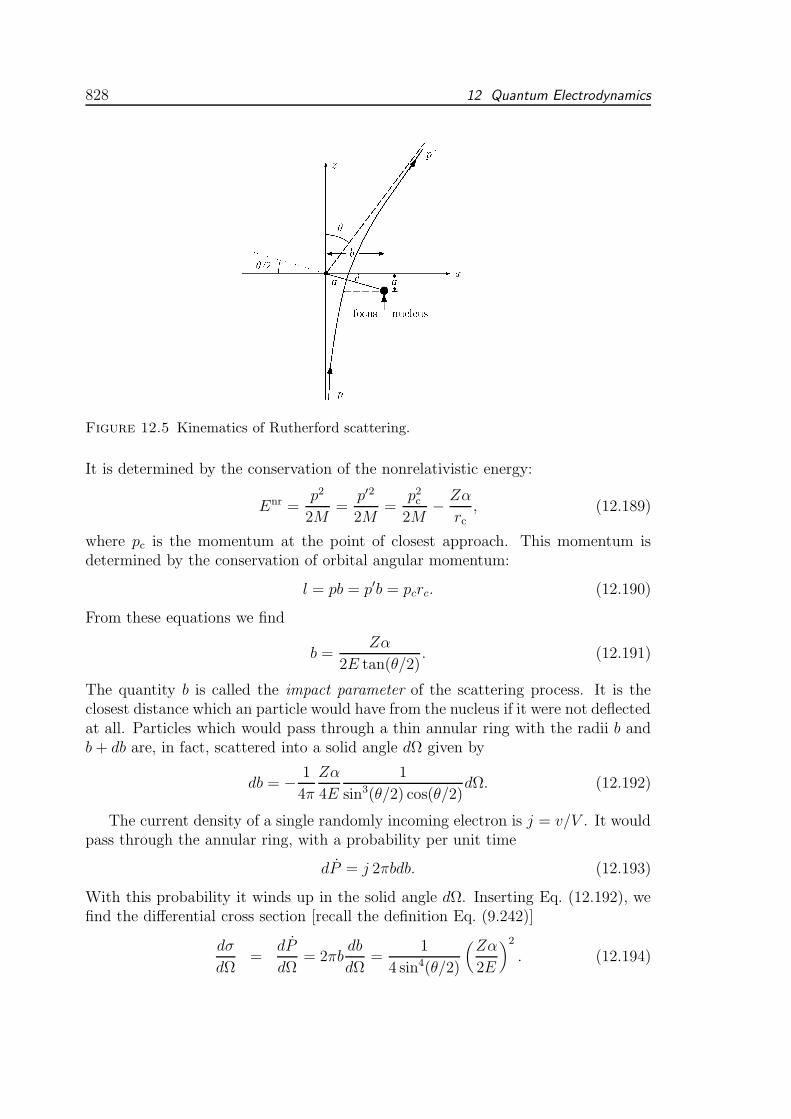
828 12 Quantum Electrodynamics
Figure 12.5 Kinematics of Rutherford scattering.
It is determined by the conservation of the nonrelativistic energy:
Enr =p2
2M=
p′2
2M=
p2c2M
− Zα
rc, (12.189)
where pc is the momentum at the point of closest approach. This momentum isdetermined by the conservation of orbital angular momentum:
l = pb = p′b = pcrc. (12.190)
From these equations we find
b =Zα
2E tan(θ/2). (12.191)
The quantity b is called the impact parameter of the scattering process. It is theclosest distance which an particle would have from the nucleus if it were not deflectedat all. Particles which would pass through a thin annular ring with the radii b andb+ db are, in fact, scattered into a solid angle dΩ given by
db = − 1
4π
Zα
4E
1
sin3(θ/2) cos(θ/2)dΩ. (12.192)
The current density of a single randomly incoming electron is j = v/V . It wouldpass through the annular ring, with a probability per unit time
dP = j 2πbdb. (12.193)
With this probability it winds up in the solid angle dΩ. Inserting Eq. (12.192), wefind the differential cross section [recall the definition Eq. (9.242)]
dσ
dΩ=
dP
dΩ= 2πb
db
dΩ=
1
4 sin4(θ/2)
(
Zα
2E
)2
. (12.194)

12.8 Rutherford Scattering 829
12.8.2 Quantum-Mechanical Born Approximation
Somewhat surprisingly, the same result is obtained in quantum mechanics within theBorn approximation. According to Eqs. (9.147) and (9.248), the differential crosssection is
dσ
dΩ≈ M2V 2
(2π)2|Vp′p|2, (12.195)
where
Vp′p = − 1
V
∫
d3x ei(p′−p)xZα
r= −4π
V
Zα
|q2|2 . (12.196)
The quantity
q2 ≡ |p′ − p|2 = 2p2(1− cos θ) = 4p2 sin2(θ/2) = 8EM sin2(θ/2) (12.197)
is the momentum transfer of the process. Inserting this into (12.196), the differentialcross section (12.195) coincides indeed with the classical expression (12.194).
12.8.3 Relativistic Born Approximation: Mott Formula
Let us now see how the above cross section formula is modified in a relativisticcalculation involving Dirac electrons. The scattering amplitude is, according toEq. (10.142),
Sfi = −ie〈p′, s′3|∫
d4x ψ(x)γµψ(x)|p, s3〉Aµ(x), (12.198)
where Aµ(x) has only the time-like component
A0(x) = − Ze
4πr= −
∫ d3q
(2π)3eiqx
Ze
|q|2 . (12.199)
The time-ordering operator has been dropped in (12.198) since there are no operatorsat different times to be ordered in first-order perturbation theory. By evaluating thematrix element of the current in (12.198), and performing the spacetime integral weobtain
Sfi = i2πδ(E ′ − E)
√
M2
V 2E ′Eu(p′, s′3)γ
0u(p, s3)Ze2
|q|2 , (12.200)
where E and E ′ are the initial and final energies of the electron, which are in factequal in this elastic scattering process.
Comparing this with (9.130) we identify the T -matrix elements
Tp′p =M
VEu(p′, s′3)γ
0u(p, s3)Ze2
|q|2 , (12.201)
In the nonrelativistic limit this is equal to
Tp′p = − 1
V
Ze2
|q|2 . (12.202)

830 12 Quantum Electrodynamics
Its relativistic extension contains a correction factor
C =M
Eu(p′, s3)γ
0u(p, s3). (12.203)
Its absolute square multiplies the nonrelativistic differential cross section (12.194).Apart from this, the relativistic cross section contains an extra kinematic factorE2/M2 accounting for the different phase space of a relativistic electron with respectto the nonrelativistic one [the ratio between (9.247) and (9.244)]. The differentialcross section (12.194) receives therefore a total relativistic correction factor
E2
M2|C|2 = |u(p′, s′3)γ
0u(p, s3)|2. (12.204)
If we consider the scattering of unpolarized electrons and do not observe the finalspin polarizations, this factor has to be summed over s′3 and averaged over s3, andthe correction factor is
E2
M2|C|2 = 1
2
∑
s′3,s3
u(p′, s′3)γ0u(p, s3)u(p, s3)γ
0u(p′, s′3). (12.205)
To write the absolute square in this form we have used the general identity in thespinor space, valid for any 4× 4 spinor matrix M :
(u′Mu)∗ = uMu′, (12.206)
where the operation bar is defined for a spinor matrix in complete analogy to thecorresponding operation for a spinor:
M ≡ γ0M †γ0−1. (12.207)
The Dirac matrices themselves satisfy
γµ = γµ. (12.208)
The “bar” operation has the typical property of an “adjoining” operation. If it isapplied to a product of matrices, the order is reversed:
M1 · · ·Mn =Mn · · ·M1. (12.209)
We use now the semi-completeness relation (4.702) for the u-spinors and rewrite(12.205) as
E2
M2|C|2 = 1
2tr
(
γ0/p +M
2Mγ0/p +M
2M
)
. (12.210)
The trace over product of gamma matrices occurring in this expression is typicalfor quantum electrodynamic calculations. Its evaluation is somewhat tedious, butfollows a few quite simple algebraic rules.
12.8 Rutherford Scattering 831
The first rule states that a trace containing an odd number of gamma matricesvanishes. This is a simple consequence of the fact that γµ and any product of anodd number of gamma matrices change sign under the similarity transformationγ5γ
µγ5 = −γµ, while the trace is invariant under any similarity transformation.The second rule governs the evaluation of a trace containing an even number of
gamma matrices. It is a recursive rule which makes essential use of the invarianceof the trace under cyclic permutations
tr(γµ1γµ2γµ3 · · · γµn−1γµn) = tr(γµ2γµ3 · · · γµn−1γµnγµ1). (12.211)
This leads to an explicit formula that is a close analog of Wick’s expansion formulafor time-ordered products of fermion field operators. To find this, we define a paircontraction between /a and /b as
/a/b ≡ 1
4tr(/a /b ) = ab. (12.212)
Then we consider a more general trace
1
4tr(/a 1 · · · /a n) (12.213)
and move the first gamma matrix step by step to the end, using the anticommutationrules between gamma matrices (4.566), which imply that
/a1/a i = −/ai /a1 + 2a1ai = −/ai /a1 + 2 /a1/ai . (12.214)
Having arrived at the end, it can be taken back to the front, using the cyclic invari-ance of the trace. This produces once more the initial trace, except for a minus sign,thus doubling the initial trace on the left-hand side of the equation if n is even. Inthis way, we find the recursion relation
1
4tr(/a1 /a2 /a3 · · · /an−1 /an ) =
1
4tr(/a1/a2) +
1
4tr(/a1/a2/a3 · · · /an−1 /an )
+ . . .+1
4tr(/a1/a2/a3 · · ·/an−1 /an ) + . . .+
1
4tr(/a1/a2/a3 · · · /an−1/an).(12.215)
The contractions within the traces are defined as in (12.212), but with a minus signfor each permutation necessary to bring the Dirac matrices to adjacent positions.Performing these operations, the result of (12.215) is
1
4tr(/a1 /a2 /a3· · · /an−1 /an )=(a1a2)
1
4tr(/a3 /a4· · · /an−1 /an ) + (a1a3)
1
4tr(/a2 /a4· · · /an−1 /an )
+ . . .+ (a1an−1)1
4tr(/a2 /a3 · · · /an−2 /an ) + (a1an)
1
4tr(/a2 /a3 · · · /an−1 /an ).(12.216)
By applying this formula iteratively, we arrive at the expansion rule of the Wicktype:
1
4tr(/a1 · · · /an ) =
∑
pair contractions
(−)P (ap(1)ap(2))(ap(3)ap(4)) · · · (ap(n−1)ap(n)), (12.217)

832 12 Quantum Electrodynamics
where P is the number of permutations to adjacent positions.The derivation of the rule is completely parallel to that of the thermodynamic
version of Wick’s rule in Section 4.14, whose Eqs. (7.857) and (7.858) can directlybe translated into anticommutation rules between gamma matrices and the cyclicinvariance of their traces, respectively.
Another set of useful rules following from (12.214) and needed later is
γµ/a γν = /a + 2aµγν , (12.218)
γµγµ = 4, (12.219)
γµ/a γµ = −2/a , (12.220)
γµ/a /b γµ = −2/a , (12.221)
γµ/a /b /b γµ = −2/c /b /a . (12.222)
Following the Wick rule (12.253) for γ-matrices, we now calculate the expression(12.210) as
E2
M2|C|2 =
1
2M2
[
1
4tr(γ0/p γ0/p ′) +M2tr(γ02)
]
=1
2M2
(
2p0p′0 − pp′ +M2)
. (12.223)
Inserting p0 = p′0 = E and, in the center-of-mass frame,
pp′ = E2 − |p|2 cos θ =M2 + 2|p|2 sin2 θ
2, (12.224)
the total cross section in the center-of-mass frame becomes
dσ
dΩCM
=Z2α2M2
4|p|4 sin4(θ/2)× E2
M2|C|2. (12.225)
This relativistic version of Rutherford’s formula is known as Mott’s formula.In terms of the incident electron velocity, the total modification factor reads
E2
M2|C|2 = 1
1− (v/c)2
[
1−(
v
c
)2
sin2 θ
2
]
. (12.226)
It is easy to verify that the same differential cross section is valid for positrons. Inthe nonrelativistic case, this follows directly from the invariance of (12.195) undere → −e. But also the relativistic correction factor remains the same under theinterchange of electrons and positrons, where (12.205) becomes
E2
M2|C|2 = 1
2
∑
s′3,s3
v(p′, s′3)γ0v(p, s3)v(p, s3)γ
0v(p′, s′3). (12.227)
Inserting the semi-completeness relation (4.703) for the spinors v(p, s3), this becomes
E2
M2|C|2 = 1
2tr
(
γ0/p −M
2Mγ0/p ′ −M
2M
)
, (12.228)
which is the same as (12.205), since only traces of an even number of gamma matricescontribute.

12.9 Compton Scattering 833
12.9 Compton Scattering
A simple scattering process, whose cross section can be calculated to a good accu-racy by means of the above diagrammatic rules, is photon-electron scattering, alsoreferred to as Compton scattering. It gives an important contribution to the bluecolor of the sky.1
Consider now a beam of photons with four-momentum ki and polarization λiimpinging upon an electron target of four-momentum pi and spin orientation σi.The two particles leave the scattering regime with four-momenta kf and pf , and spinindices λf , σf , respectively. Adapting formula (10.103) for the scattering amplitudeto this situation we have
Sfi = S (p′, s′3;k′, h′|k, h;p, s3)
≡ 〈0|a(p′, s′3)a(k′, h′)T e
−i∫
∞
−∞dtVI (t)a†(k, h)a†(p, s3)|0〉
〈0|e−i∫
∞
−∞dtVI (t)|0〉
≡ SN (p′, s′3;k′, h′|k, h;p, s3) /Z[0], (12.229)
with
e−i∫
∞
−∞dt VI(t) = e−ie
∫
d4x ψ(x)γµψ(x)Aµ(x). (12.230)
Expanding the exponential in powers of e, we see that the lowest-order contributionto the scattering amplitude comes from the second-order term which gives rise to thetwo Feynman diagrams shown in Fig. 12.6. In the first, the electron s1 of momentump absorbs a photon of momentum k, and emits a second photon of momentum k′,to arrive in the final state of momentum p′. In the second diagram, the acts ofemission and absorption have the reversed order. Before we calculate the scatteringcross section associated with these Feynman diagrams, let us first recall the classicalresult.
Figure 12.6 Lowest-order Feynman diagrams contributing to Compton Scattering and
giving rise to the Klein-Nishina formula.
1The blue color is usually attributed to Rayleigh scattering. This arises from generalizing Thom-son’s formula (12.233) for the scattering of light of wavelength λ on electrons to that on dropletsof diameter d with refractive index n. That yields σRayleigh = 2π5d6[(n2 − 1)/(n2 + 2)]2/3λ4.

834 12 Quantum Electrodynamics
12.9.1 Classical Result
Classically, the above process is described as follows. A target electron is shakenby an incoming electromagnetic field. The acceleration of the electron causes anemission of antenna radiation. For a weak and slowly oscillating electromagneticfield of amplitude, the electron is shaken nonrelativistically and moves with aninstantaneous acceleration
x =e
ME =
e
ME0e
−iωt+ik·x, (12.231)
where ω is the frequency and E0 the amplitude of the incoming field.The acceleration of the charge gives rise to antenna radiation following Larmor’s
formula. Inserting (12.231) into (5.37), and averaging over the temporal oscillations,the radiated power per unit solid angle is
dEdΩ
=1
2
(
e2
4πM
)2
E20 sin
2 β, (12.232)
where β is the angle between the direction of polarization of the incident light andthe direction of the emitted light.
For a later comparison with quantum electrodynamic calculations we associatethis emitted power with a differential cross section of the electron with respect tolight. According to the definition in Chapter 6, a cross section is obtained by dividingthe radiated power per unit solid angle by the incident power flux density cE2
0/2.This yields
dσ
dΩ=
(
e2
4πMc2
)2
sin2 β = r2e sin2 β, (12.233)
where
re =e2
4πMc2=
hα
Mc≈ 2.82× 10⁻¹³ cm (12.234)
is the classical electron radius. Formula (12.233) describes the so-called Thomson
scattering cross section. It is applicable to linearly polarized incident waves. Forunpolarized waves, we have to form the average between the cross section (12.233)and another one in which the plane of polarization is rotated by 90%. Supposethe incident light runs along the z-axis, and the emitted light along the directionk = (sin θ cos φ, sin θ sin φ, cos θ). For a polarization direction = ˆx along the x-axis,the angle β is found from
sin2 β = (k× )2 = cos2 θ + sin2 θ sin2 φ. (12.235)
For a polarization direction = ˆx along the y-axis, it is
sin2 β = (k× )2 = cos2 θ + sin2 θ cos2 φ. (12.236)
The average is
sin2 β = cos2 θ +1
2sin2 θ =
1
2(1 + cos2 θ). (12.237)

12.9 Compton Scattering 835
Integrating this over all solid angles yields the Thomson cross section for unpolarizedlight
σtot =8π
3r2e . (12.238)
12.9.2 Klein-Nishina Formula
The scattering amplitude corresponding to the two Feynman diagrams in Fig. 12.6is obtained by expanding formula (10.103) up to second order in e:
Sfi = −e2∫
d4xd4y〈0|ap′,s′3T ψ(y)/ǫ ′ψ(y)ψ(x)/ǫ ψ(x)a†p,s3|0〉, (12.239)
and by performing the Wick contractions of Section 7.8:
〈0|ap′,s′3T ψ(y)/ǫ ′ψ(y)ψ(x)/ǫ ψ(x)a†p,s3|0〉 = 〈0|T ap′,s′
3ψ(y) /ǫ ′ ψ(y)ψ(x) /ǫ ψ(x)a†p,s3 |0〉
+〈0|T ap′,s′3ψ(y)/ǫ′ψ(y)ψ(x)/ǫψ(x)a†p,s3 |0〉|0〉. (12.240)
After Fourier-expanding the intermediate electron propagator,
G0(y, x) =∫
d4pi
(2π)4e−ip
i(y−x) i
/p i −M, (12.241)
we find
Sfi = −e2∫
d4xd4yek′y−kx
∫ d4pi
(2π)4M√
V 2EE ′2ω2ω′
×[
ei(p′−pi)y−(p−pi)xu(p′, s′3)/ǫ
′∗ i
/p i −M/ǫ u(p, s3)
+ ei(p′−pi)x−(p−pi)yu(p′, s′3)/ǫ
i
/p i −M/ǫ ′u(p, s3)
]
. (12.242)
One of the spatial integrals fixes the intermediate momentum in accordance withenergy-momentum conservation, the other yields a δ(4)-function for overall energy-momentum conservation. The result is
Sfi = −i(2π)4δ(4)(p′ + k′ − p− k)e2M√
V 2EE ′2ω2ω′u(p′, s′3)Hu(p, s3), (12.243)
where H is the 4× 4-matrix in spinor space
H ≡ /ǫ ′∗(/p + /k ) +M
(p+ k)2 −M2/ǫ + /ǫ
(/p − /k ′) +M
(p− k′)2 −M2/ǫ ′∗. (12.244)
We have written ǫ(k, h), ωk as ǫ, ω, and ǫ(k′, h′), ωk′ as ǫ′, ω′, respectively, with asimilar simplification for E and E ′. The second term of the matrix H arises fromthe first by the crossing symmetry
ǫ↔ ǫ′, k ↔ −k′. (12.245)

836 12 Quantum Electrodynamics
Simplifications arise from the properties (12.246). It can, moreover, be simplifiedby recalling that external electrons and photons are on their mass shell, so that
p2 = p′2 =M2, k2 = k′2 = 0, (12.246)
k ǫ = k′ǫ′ = 0. (12.247)
A further simplification arises by working in the laboratory frame in which the initialelectron is at rest, p = (M, 0, 0, 0). Also, we choose a gauge in which the polarizationvectors have only spatial components. Then
p ǫ = p ǫ′ = 0, (12.248)
since p has only a temporal component and ǫ only space components. We alsouse the fact that H stands between spinors which satisfy the Dirac equation (/p −M)u(p, s3) = 0, u(p, s3)(/p −M) = 0. Further we use the commutation rules (4.566)for the gamma matrices to write [as in (12.214)]
/p/ǫ = − /ǫ/p + 2pǫ. (12.249)
The second term vanishes by virtue of Eq. (12.248). Similarly, we see that /p anti-commutes with /ǫ ′. Using these results, we may eliminate the terms /p +M occurringin M . Finally, using Eq. (12.247), we obtain
u(p′, s′3)Hu(p, s3) = u(p′, s′3)
ǫ′∗/k
2pk/ǫ + /ǫ
/k ′
2pk′/ǫ ′∗
u(p, s3). (12.250)
To obtain the transition probability, we must take the absolute square of this. Ifwe do not observe initial and final spins, we may average over the initial spin andsum over the final spin directions. This produces a factor 1/2 times the sum overboth spin directions, which is equal to
F =∑
s′3,s3
|u(p′, s′3)Hu(p, s3)|2 =∑
s′3,s3
u(p′, s′3)Hu(p, s3)u(p, s3)Hu(p′, s′3). (12.251)
Here we apply the semi-completeness relation (4.702) for the spinors to find
F =1
4M2tr [(/p ′ +M)H(/p +M)H ] . (12.252)
The trace over the product of gamma matrices can be evaluated according to theWick-type of rules explained on p. 830.
1
4tr(/a 1 · · · /a n) =
∑
pair contractions
(−)P /a 1 · · · /a n. (12.253)
After some lengthy algebra (see Appendix 9A), we find
F =1
2M2
[
ω′
ω+ω
ω′− 2 + 4|′∗ · |2
]
. (12.254)

12.9 Compton Scattering 837
Figure 12.7 Illustration of the photon polarization sum∑
h,h′ |′∗|2 = 1 + cos2 θ in
Compton scattering in the laboratory frame. Incoming and outgoing photon momenta
with scattering angle θ are shown in the scattering plane, together with their transverse
polarization vectors.
This holds for specific polarizations of the incoming and outgoing photons. If we sumover all final polarizations and average over all initial ones, we find (see Fig. 12.7)
1
2
∑
h,h′|′∗|2 = 1
2(1 + cos2 θ), (12.255)
This can also be found more formally using the transverse completeness relation(4.334) of the polarization vectors:
1
2
∑
h,h′|′∗|2= 1
2
∑
h,h′ǫ′i∗(k′, h′)ǫi(k, h)ǫ∗j(k, h)ǫ′i(k′, h′) (12.256)
=1
2
(
δij − kikj
k2
)(
δji − k′jk′i
k′2
)
=1
2
[
1 +(k · k′)2
k2k′2
]
=1
2(1 + cos2 θ).
The average value of F is therefore
F =1
2
∑
h,h′
1
2M2
[
ω′
ω+ω
ω′− 2 + 4|′∗ · |2
]
=1
M2
[
ω′
ω+ω
ω′− sin2 θ
]
. (12.257)
We are now ready to calculate the transition rate, for which we obtain fromEq. (9.298):
dP
dt= V (2π)4
∫ d3p′V
(2π)3
∫ d3k′V
(2π)3δ(4)(p′ − p)|tfi|2, (12.258)
with the squared t-matrix elements
|tfi|2 = e41
V 4
M2
EE ′2ω2ω′
1
2F. (12.259)
The spatial part of the δ-function removes the momentum integral over p′. Thetemporal part of the δ-function enforces energy conservation. This is incorporatedinto the momentum integral over k′ as follows. We set Ef = p′0 + k′0, and write
d3k′ = k′2dk′dΩ = ω′2 dω′
dEf
dΩdEf , (12.260)

838 12 Quantum Electrodynamics
where Ω is the solid angle into which the photon has been scattered. Then (12.258)becomes
dP
dtdΩ= V e4(2π)4
V 2
(2π)6
(
ω′
ω
)
dω′
dEf
∣
∣
∣
∣
∣
Ef=Ei
1
4V 4
M2
EE ′
1
2F. (12.261)
For an explicit derivative dω′/dEf , we go to the laboratory frame and express thefinal energy as
Ef = ω′+√
p′2 +M2 = ω′+√
(k− p′)2 +M2 = ω′+√ω2 − 2ωω′ cos θ + ω′2 +M2,
(12.262)where θ is the scattering angle in the laboratory. This yields the derivative
dEf
dω′= 1 +
ω′ − ω cos θ
E ′. (12.263)
By equating Ei =M + ω with Ef , we derive the Compton relation
ωω′(1− cos θ) =M(ω − ω′), (12.264)
orω′ =
ω
1 + ω(1− cos θ)/M, (12.265)
and therefore
dEf
dω′= 1 +
ω′ − ω cos θ
E ′=E ′ + ω′ − ω cos θ
E ′=M + ω − ω cos θ
E ′=M
E ′
ω
ω′. (12.266)
Since E =M in the laboratory frame, Eq. (12.261) yields the differential probabilityrate
dP
dtdΩ= V e4(2π)4
V 2
(2π)6V
(
ω′
ω
)21
4V 4
1
2F. (12.267)
To find the differential cross section, this has to be divided by the incomingparticle current density. According to Eq. (9.315), this is given by
j =v
V, (12.268)
where v is the velocity of the incoming particles. The incoming photons move withlight velocity, so that (in natural units with c = 1)
j =1
V. (12.269)
This leaves us with the Klein-Nishina formula for the differential cross section
dσ
dΩ= α2
(
ω′
ω
)21
2F. (12.270)

12.10 Electron-Positron Annihilation 839
In the nonrelativistic limit where ω ≪ M , the Compton relation (12.265) showsthat ω′ ≈ ω, and Eq. (12.257) reduces to
F → 1
M2(1 + cos2 θ). (12.271)
Expressed in terms of the classical electron radius r0 = α/M , the differential scat-tering cross section becomes, expressed in terms of the classical electron radiusr0 ≡ α/M ,
dσ
dΩ≈ r0
2 1
2(1 + cos2 θ). (12.272)
This is the Thomson formula for the scattering of low energy radiation by a staticcharge. To find the total Thomson cross section, we must integrate (12.272) over allsolid angles and obtain:
σ =∫
dΩdσ
dΩ≈ 2π
∫ 1
−1d cos θ r20
1
2(1 + cos2 θ). (12.273)
In the low-energy limit we identify
σThomson ≡ r028π
3. (12.274)
Let us also calculate the total cross section for relativistic scattering, integrating(12.270) over all solid angles:
σ =∫
dΩdσ
dΩ= 2π
∫ 1
−1d cos θ
α2
2M2
(
ω′
ω
)2 [ω′
ω+ω
ω′− sin2 θ
]
. (12.275)
Inserting
ω′ =ω
1 + ω(1− cos θ)/M, (12.276)
which follows from (12.265), the angular integral yields
σ = σThomsonf(ω), (12.277)
where f(ω) contains the relativistic corrections to Thomson’s cross section:
f(ω) =3
8ω3
2ω[ω(ω + 1)(ω + 8) + 2]
(2ω + 1)2− (2+2ω−ω2) log(1 + 2ω)
(12.278)
For small ω, f(ω) starts out like (see Fig. 12.8a):
f(ω) = 1− 2ω +O(ω2). (12.279)
For large ω, ωf(ω) increases like (see Fig. 12.8b):
ωf(ω) =3
8ωlog 2ω +O(1/ logω). (12.280)
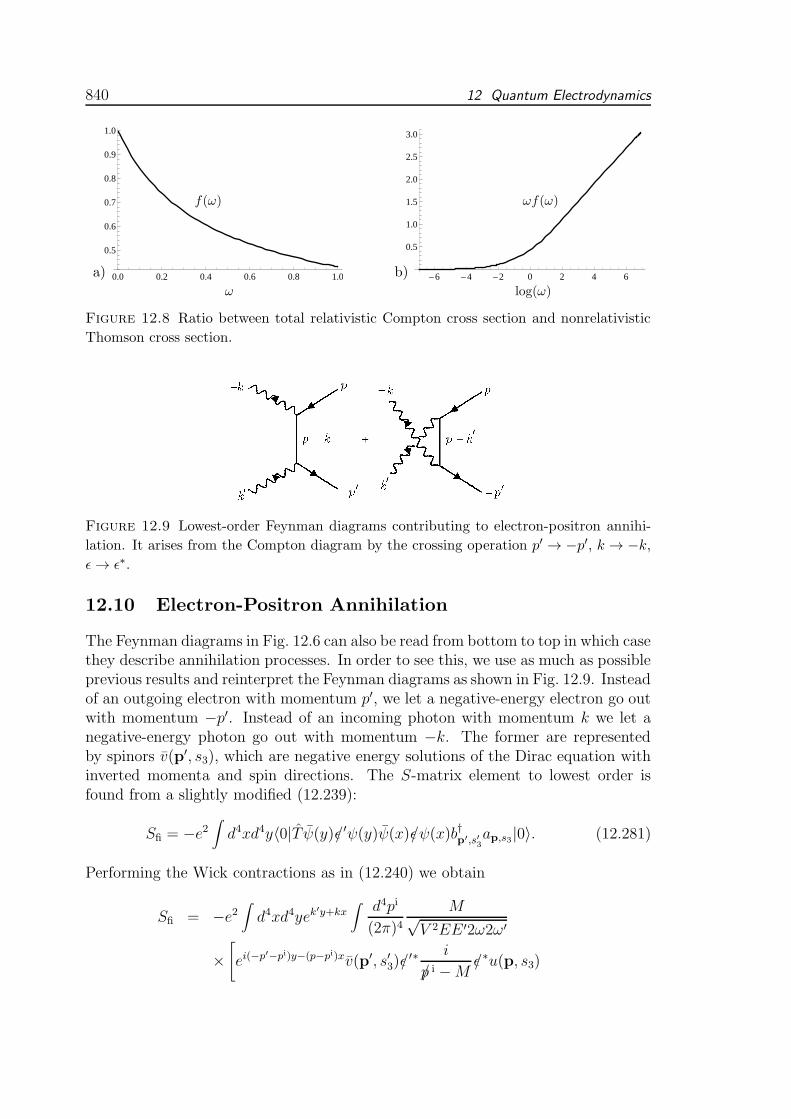
840 12 Quantum Electrodynamics
-6 -4 -2 0 2 4 6
0.5
1.0
1.5
2.0
2.5
3.0
ωf(ω)
log(ω)
b)0.0 0.2 0.4 0.6 0.8 1.0
0.5
0.6
0.7
0.8
0.9
1.0
f(ω)
ω
a)
Figure 12.8 Ratio between total relativistic Compton cross section and nonrelativistic
Thomson cross section.
Figure 12.9 Lowest-order Feynman diagrams contributing to electron-positron annihi-
lation. It arises from the Compton diagram by the crossing operation p′ → −p′, k → −k,
ǫ → ǫ∗.
12.10 Electron-Positron Annihilation
The Feynman diagrams in Fig. 12.6 can also be read from bottom to top in which casethey describe annihilation processes. In order to see this, we use as much as possibleprevious results and reinterpret the Feynman diagrams as shown in Fig. 12.9. Insteadof an outgoing electron with momentum p′, we let a negative-energy electron go outwith momentum −p′. Instead of an incoming photon with momentum k we let anegative-energy photon go out with momentum −k. The former are representedby spinors v(p′, s3), which are negative energy solutions of the Dirac equation withinverted momenta and spin directions. The S-matrix element to lowest order isfound from a slightly modified (12.239):
Sfi = −e2∫
d4xd4y〈0|T ψ(y)/ǫ ′ψ(y)ψ(x)/ǫ ψ(x)b†p′,s′
3
ap,s3|0〉. (12.281)
Performing the Wick contractions as in (12.240) we obtain
Sfi = −e2∫
d4xd4yek′y+kx
∫
d4pi
(2π)4M√
V 2EE ′2ω2ω′
×[
ei(−p′−pi)y−(p−pi)xv(p′, s′3)/ǫ
′∗ i
/p i −M/ǫ ∗u(p, s3)

12.10 Electron-Positron Annihilation 841
+ ei(−p′−pi)x−(p−pi)y v(p′, s′3)/ǫ
∗ i
/p i −M/ǫ ′u(p, s3)
]
. (12.282)
Note that this arises from the Compton expression (12.242) by the crossing opera-tion
p′ → −p′, u(p, s3) → v(p, s3), k → −k, ǫ(k, h) → ǫ∗(k, h). (12.283)
As before, one of the spatial integrals fixes the intermediate momentum in accor-dance with energy-momentum conservation, the other yields a δ(4)-function for over-all energy-momentum conservation. The result is
Sfi = −i(2π)4δ(4)(k + k′ − p− p′)e2M√
V 2EE ′2ω2ω′v(p′, s′3)Hu(p, s3), (12.284)
where H is the 4× 4-matrix in spinor space
H ≡ /ǫ ′∗(/p − /k ) +M
(p− k)2 −M2/ǫ ∗ + /ǫ ∗
(/p − /k ′) +M
(p− k′)2 −M2/ǫ ′∗. (12.285)
As before, we have written ǫ(k, h), ωk as ǫ, ω, and ǫ(k′, h′), ωk′ as ǫ′, ω′, respectively,with a similar simplification for E and E ′. The second term of the matrix H arisesfrom the first by the Bose symmetry
ǫ↔ ǫ′, k ↔ k′. (12.286)
Simplifications arise from the mass shell properties (12.246), the gauge conditions(12.247), and the other relations (12.248), (12.249). We also work again in thelaboratory frame in which the initial electron is at rest, p = (M, 0, 0, 0) and thepositron comes in with momentum p′ and energy E ′ =
√p′2 +M2. This leads to
v(p′, s′3)Hu(p, s3) = v(p′, s′3)
ǫ′∗/k
2pk/ǫ ∗ + /ǫ ∗
/k ′
2pk′/ǫ ′∗
u(p, s3). (12.287)
To obtain the transition probability, we must take the absolute square of this.If we do not observe initial spins, we may average over the initial spin componentswhich gives a factor 1/4 times the spin sum
F =∑
s′3,s3
|v(p′, s′3)Hu(p, s3)|2 =∑
s′3,s3
v(p′, s′3)Hu(p, s3)u(p, s3)Hu(p′, s′3). (12.288)
Now we use the semi-completeness relations (4.702) and (4.703) for the spinors torewrite (12.288) as
F = − 1
4M2tr [(−/p ′ +M)H(/p +M)H ] . (12.289)

842 12 Quantum Electrodynamics
The trace over a product of gamma matrices is now evaluated as before and weobtain, for specific polarizations of the two outgoing photons, almost the same ex-pression as before in Eq. (12.257) (see Appendix 12A):
F =1
2M2
[
ω′
ω+ω
ω′+ 2− 4|′∗ · ∗|2
]
. (12.290)
This result can be deduced directly from the previous polarization sum (12.254) bythe crossing operation (12.283), apart from an overall minus sign, whose origin isthe negative sign in front of (12.289).
We are now ready to calculate the transition rate, for which we obtain fromEq. (9.298)
dP
dt= V (2π)4
∫
d3k′V
(2π)3
∫
d3k′V
(2π)3δ(4)(p′ − p)|tfi|2, (12.291)
with the squared t-matrix elements
|tfi|2 = e41
V 4
M2
EE ′2ω2ω′
1
4F. (12.292)
The spatial part of the δ-function removes the momentum integral over k′. Thetemporal part of the δ-function enforces energy conservation. This is incorporatedinto the momentum integral over k as follows. We set Ef = ω + ω′, and write
d3k = k2dkdΩ = ω2 dω
dEfdΩdEf , (12.293)
where Ω is the solid angle into which the photon with momentum k emerges. Then(12.291) becomes
dP
dtdΩ= V e4(2π)4
V 2
(2π)6
(
ω
ω′
)
dω
dEf
∣
∣
∣
∣
∣
Ef=Ei
1
4V 4
M2
EE ′
1
4F. (12.294)
To calculate dω/dEf explicitly, we express the final energy in the laboratory frameas
Ef = ω +√k′2 = ω +
√
(p′ − k)2 = ω +√
p′2 − 2ω|p′| cos θ + ω2, (12.295)
where θ is the scattering angle in the laboratory. Hence:
dEf
dω=1 +
1
2ω′
d
dω
(
p′2 − 2ω|p′| cos θ + ω2)
=1
ωω′
(
ωω′ − 2ω|p′| cos θ + ω2)
=1
ωω′
[
ω(
M +√
p′2+M2
)
−2ω|p′| cos θ]
=k(p+ p′)
ωω′=M(M + E ′)
ωω′. (12.296)
We must now divide (12.294) by the incoming positron current density j = |p′|/E ′V[recall (9.315)], and find the differential cross section
dσ
dΩ=
α2
|p′|(M + E ′)
(
ω
M
)2 1
4M2F, (12.297)

12.10 Electron-Positron Annihilation 843
Figure 12.10 Illustration of the photon polarization sum∑
h,h′ |′∗|2 in electron-
positron annihilation in the laboratory frame. Incoming positron and outgoing photon
momenta with scattering angles θ and θ′ are shown in the scattering plane, together with
their transverse polarization vectors.
whereM
ω=M + E ′ − |p′| cos θ
M + E ′, (12.298)
as follows from equating the right-hand sides of
kk′ =1
2(k + k′)2 =
1
2(p+ p′)2 =M(M + E ′), (12.299)
andkk′ = k(p + p′ − k) = ω(M + E ′ − |p′| cos θ). (12.300)
If the incoming positron is very slow, then ω ≈ ω′ ≈M , and the two photons shareequally the rest energies of the electron and the positron. We can now substitute inF of Eq. (12.290):
ω′
ω=E ′ − |p′|cos θ
M, (12.301)
and sum over all photon polarizations to obtain [see Fig. 12.10 and Eq. (12.257)]
∑
h,h′|′∗|2 = 1 +
(k · k′)2
k2k′2= 1 + cos2(θ + θ′) =
(
1− M
ω− M
ω′
)2
. (12.302)
The last expression is found by observing that
k k′ = ωω′[1− cos(θ + θ′)], (12.303)
so that we can express
cos(θ + θ′) = 1− k k′
ωω′= 1− 1
2
(k + k′)2
ωω′= 1− 1
2
(p+ p′)2
ωω′= 1− M(M + E ′)
ωω′.
Energy conservation leads to
cos(θ + θ′) = 1− k k′
ωω′= 1− M(ω + ω′)
ωω′, (12.304)
thus obtainig the right-hand side of (12.302). Note that from (12.303) and (12.304)we find a relation
k k′ =M(ω + ω′). (12.305)

844 12 Quantum Electrodynamics
We now introduce the relativistic factor of the incoming positron γ ≡ E ′/M andwrite the relation (12.298) as
M
ω= 1−
√
γ − 1
γ + 1cos θ,
M
ω′=
1−√
γ − 1
γ + 1cos θ
γ −√γ2 − 1 cos θ
. (12.306)
The result is integrated over all solid angles, and divided by 2 to account for Bosestatistics of the two final photons. This yields the cross section expressed in termsof the classical electron radius r0 = α/M :
σ(γ) =1
2
∫
dΩdσ
dΩ=
πr201 + γ
[
γ2 + 4γ + 1
γ2 − 1log
(
γ +√
γ2 − 1)
− γ + 3√γ2 − 1
]
.
(12.307)For small incoming positron energy, the cross section diverges like
σ(γ)−−−→smallp
σlow−energy(γ) ≡πr20 γ√γ2 − 1
≈ πr20c
v, (12.308)
whereas in the high-energy limit it behaves like
σ−−−→|p|→∞
πr20γ
[log(2γ)− 1] . (12.309)
The detailed behavior is shown in Fig. 12.11.
The above result can be used to estimate the lifetime of a positron movingthrough matter. We simply have to multiply the cross section σ by the incidentcurrent density j = |p|/EV of a single positron and by the number N of targetelectrons, which is Z per atom. For slow positrons we may use Eq. (12.308) to findthe decay rate
1. 2. 3. 4. 5. 6. 7. 8. 9. 10.
0.2
0.4
0.6
0.8
1.
γ
σ(γ)/σ low−energy(γ)
Figure 12.11 Electron-positron annihilation cross section divided by its low-energy lim-
iting expression (12.308) as a function of γ = 1/√
1− v2/c2 of the incoming positron in
the laboratory frame.
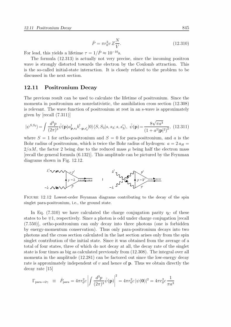
12.11 Positronium Decay 845
P = πr20v ZN
V. (12.310)
For lead, this yields a lifetime τ = 1/P ≈ 10−10s.The formula (12.313) is actually not very precise, since the incoming positron
wave is strongly distorted towards the electron by the Coulomb attraction. Thisis the so-called initial-state interaction. It is closely related to the problem to bediscussed in the next section.
12.11 Positronium Decay
The previous result can be used to calculate the lifetime of positronium. Since themomenta in positronium are nonrelativistic, the annihilation cross section (12.308)is relevant. The wave function of positronium at rest in an s-wave is approximatelygiven by [recall (7.311)]
|ψS,S3〉=∫ d3p
(2π)3ψ(p)a†p,s3b
†−p,s′
3|0〉〈S, S3|s, s3; s, s′3〉, ψ(p)=
8√πa3
(1 + a2|p|2)2, (12.311)
where S = 1 for ortho-positronium and S = 0 for para-positronium, and a is theBohr radius of positronium, which is twice the Bohr radius of hydrogen: a = 2 aH =2/αM , the factor 2 being due to the reduced mass µ being half the electron mass[recall the general formula (6.132)]. This amplitude can be pictured by the Feynmandiagrams shown in Fig. 12.12.
Figure 12.12 Lowest-order Feynman diagrams contributing to the decay of the spin
singlet para-positronium, i.e., the ground state.
In Eq. (7.310) we have calculated the charge conjugation parity ηC of thesestates to be ∓1, respectively. Since a photon is odd under charge conjugation [recall(7.550)], ortho-positronium can only decay into three photons (one is forbiddenby energy-momentum conservation). Thus only para-positronium decays into twophotons and the cross section calculated in the last section arises only from the spinsinglet contribution of the initial state. Since it was obtained from the average of atotal of four states, three of which do not decay at all, the decay rate of the singletstate is four times as big as calculated previously from (12.308). The integral over allmomenta in the amplitude (12.281) can be factored out since the low-energy decayrate is approximately independent of v and hence of p. Thus we obtain directly thedecay rate [15]
Γpara→2γ ≡ Ppara = 4πr20c
∣
∣
∣
∣
∣
∫
d3p
(2π)3ψ(p)
∣
∣
∣
∣
∣
2
= 4πr20c |ψ(0)|2 = 4πr20c1
πa3

846 12 Quantum Electrodynamics
=Mc2
h
α5
2. (12.312)
Using the electron energy Mc2 ≈ 0.510 MeV and the Planck constant h ≈ 6.682×10⁻¹⁶eV s, the ratio h/Mc2 is equal to 1.288 × 10⁻²² s. Together with the factor2/α5, this leads to a lifetime τ = 1/Γ ≈ 0.13× 10⁻⁹ s.
The decay of the spin triplet ortho-positronium state proceeds at a roughlythousand times slower rate
Γorth→3γ ≡ Porth =Mc2
h
α6
2
4(π2 − 9)
9π, (12.313)
with a lifetime of 140× 10−9 s.
Figure 12.13 Lowest-order Feynman diagrams contributing to decay of the spin-triplet
ortho-positronium, the first excited state which lies 203.5 GHz above the ground state.
Decays into 4 and 5 photons have also been calculated and measured experimen-tally. The theoretical rates are [14, 15]:
Γpara→4γ ≈ 0.0138957Mc2
hα7[
1−14.5α
π+O(α2)
]
≈ 1.43× 10⁻⁶ × Γpara→2γ . (12.314)
Γorth→5γ ≈ 0.0189α2 × Γorth→3γ ≈ 0.959× 10⁻⁶ × Γorth→3γ. (12.315)
Experimentally, the branching ratios are 1.14(33) × 10−6 and 1.67(99) × 10−6, inreasonable agreement with the theoretical numbers. The validity of C-invariancehas also been tested by looking for the forbidden decays of para-positronium intoan odd and ortho-positronium into an even number of photons. So far, there is noindication of C-violation.
12.12 Bremsstrahlung
If a charged particle is accelerated or slowed down, it emits an electromagneticradiation called Bremsstrahlung . This is a well-known process in classical electro-dynamics and we would like to find the quantum field theoretic generalization of it.First, however, we shall recapitulate the classical case.
12.12.1 Classical Bremsstrahlung
Consider a trajectory in which a particle changes its momentum abruptly from p top′ [see Fig. 12.14].

12.12 Bremsstrahlung 847
Figure 12.14 Trajectories in the simplest classical Bremsstrahlung process: An electron
changing abruptly its momentum.
The trajectory may be parametrized as:
xµ(τ) =
τp/M
τp′/Mfor
τ < 0,
τ > 0,(12.316)
where τ is the proper time. The electromagnetic current associated with this tra-jectory is
jµ(x) = e∫
dτdxµ(τ)
dτδ(4)(x− x(τ))
=e
M
∫
dτ[
Θ(τ)pµδ(4)(x− τp/M) + θ(−τ)p′µδ(4)(x− τp′/M)]
.(12.317)
After a Fourier decomposition of the δ-functions, this can be written as
jµ(x) =∫
d4k
(2π)4e−ikxjµ(k), (12.318)
with the Fourier components
jµ(k) = −ie(
pµ
pk− p′µ
p′k
)
. (12.319)
The vector potential associated with this current is found by solving the Maxwellequation Eq. (12.50). Under the initial condition that at large negative time, thevector potential describes the retarded Coulomb potential of the incident particle,we obtain
Aµ(x) = i∫
dx′GR(x− x′)jµ(x′), (12.320)
where GR(x − x′) is the retarded Green function defined in Eq. (7.162). At verylarge times the particle has again a Coulomb field associated with it which can befound by using the advanced Green function of Eq. (7.168):
Aµout(x) = i∫
dx′GA(x− x′)jµ(x′). (12.321)
As the acceleration takes place, the particle emits radiation which is found from thedifference between the two fields,
Aµrad =1
i
∫
dx′[GR(x, x′)−GA(x, x
′)]jµ(x′). (12.322)

848 12 Quantum Electrodynamics
Remembering the list (7.212) of Fourier transforms of the various Green functions,we see that the Fourier components of the radiation field are given by
Aµrad(k) = −i2πǫ(k0)δ(k2)jµ(k). (12.323)
The energy of the electromagnetic field is, by Eq. (7.427):
H =∫
d3x1
2(−AµAµ −∇Aµ∇Aµ). (12.324)
A classical field which solves the field equations can be Fourier decomposed intopositive- and negative-frequency components as in (7.390),
Aµ(x) =∑
k
1√2V ωk
(
e−ikxaµk + eikxaµ†k)
, (12.325)
where
aµk ≡3∑
λ=0
ǫµ(k, λ)ak,λ (12.326)
are classical Fourier components. Then the combination of time and space deriva-tives in (12.324) eliminates all terms of the form akak and a∗ka
∗k, and we find
H =∑
k
ωk
2(−aµ∗k aνk − aµka
νk∗) gµν , (12.327)
just as in the calculation of the energy in (7.428). The radiation field (12.323)corresponds to
aµk = −ijµ(k)|k0=|k|. (12.328)
Inserting everything into (12.327) we derive, for large t, an emitted energy
E = −∫
d3k
2k0(2π)3k0
∑
h=1,2
j∗µ(k)jµ(k). (12.329)
Inserting (12.319) we obtain the energy emitted into a momentum space elementd3k:
dE =1
2
d3k
(2π)3e2[
2pp′
(pk)(p′k)− M2
(pk)2− M2
(p′k)2
]
, (12.330)
where polarization vectors have vanishing zeroth components. Dividing out theenergy per photon k0, this can be interpreted as the probability of omitting a photoninto d3k:
dP =d3k
2k0(2π)3e2[
2pp′
(pk)(p′k)− M2
(pk)2− M2
(p′k)2
]
. (12.331)
If we are interested in the polarization of the radiated electromagnetic field, wemake use of the local current conservation law ∂µj
µ which reads, in momentumspace,
k · j = k0j0. (12.332)

12.12 Bremsstrahlung 849
This allows us to rewrite
j∗µ(k)jµ(k) = |j0(k)|2 − |j(k)|2 = 1
k2|k · j(k)|2 − |j(k)|2 = −|jT (k)|2, (12.333)
where
jiT (k) ≡(
δij − kikj
k2
)
jj(k) (12.334)
is the transverse part of the current. In the second-quantized description of theenergy, the transverse projection is associated with a sum over the two outgoingphoton polarization vectors [recall (4.334)]:
δij −kikjk2
=∑
h=1,2
ǫ∗i (k, h)ǫi(k, h). (12.335)
The emitted energy (12.329) can therefore be resolved with respect to the polariza-tion vectors as
E =∫
d3k
2k0(2π)3k0
∑
h=1,2
|(k, h) · j(k)|2. (12.336)
This leads to an energy emitted into a momentum space element d3k:
dE =d3k
2(2π)3e2
∑
h=1,2
∣
∣
∣
∣
∣
pǫ
pk− p′ǫ
p′k
∣
∣
∣
∣
∣
2
, (12.337)
and a corresponding probability of omitting a photon into d3k, by analogy with(12.331).
Let us calculate the angular distribution of the emitted energy in Eq. (12.330).Denote the direction of k by n:
n ≡ k
|k| . (12.338)
Then we can write pk aspk = E|k|(1− v · n) (12.339)
and find
dE =d3k
(2π)32
e2
|k|2[
2(1−v · v′)
(1−v · n)(1−v′ · n) −M2
E2(1−v · n)2−M2
E ′2(1−v′ · n)2]
. (12.340)
The radiation is peaked around the directions of the incoming and outgoing particles.
12.12.2 Bremsstrahlung in Mott Scattering
We now turn to the more realistic problem of an electron scattering on a nucleus.Here the electron changes its momentum within a finite period of time rather thanabruptly. Still, the Bremsstrahlung will be very similar to the previous one. Let usconsider immediately a Dirac electron, i.e., we study the Bremsstrahlung emitted
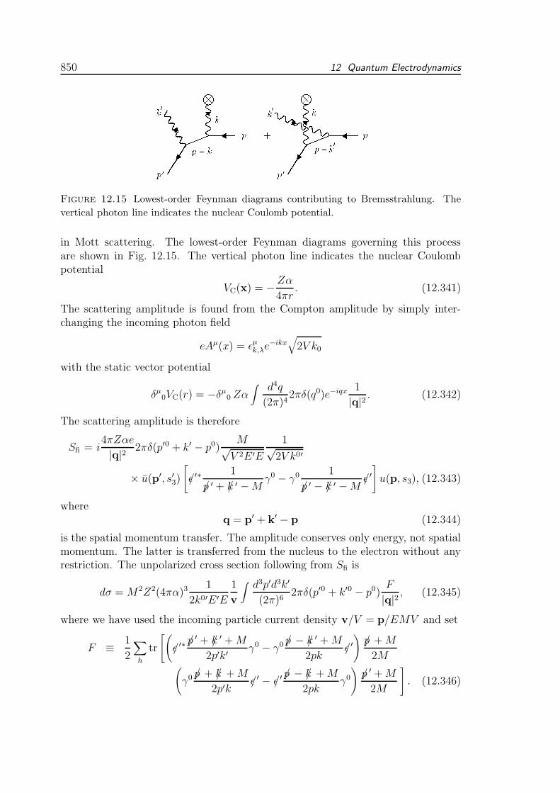
850 12 Quantum Electrodynamics
Figure 12.15 Lowest-order Feynman diagrams contributing to Bremsstrahlung. The
vertical photon line indicates the nuclear Coulomb potential.
in Mott scattering. The lowest-order Feynman diagrams governing this processare shown in Fig. 12.15. The vertical photon line indicates the nuclear Coulombpotential
VC(x) = −Zα
4πr. (12.341)
The scattering amplitude is found from the Compton amplitude by simply inter-changing the incoming photon field
eAµ(x) = ǫµk,λe−ikx
√
2V k0
with the static vector potential
δµ0VC(r) = −δµ0 Zα∫
d4q
(2π)42πδ(q0)e−iqx
1
|q|2 . (12.342)
The scattering amplitude is therefore
Sfi = i4πZαe
|q|2 2πδ(p′0 + k′ − p0)M√V 2E ′E
1√2V k0′
× u(p′, s′3)
[
/ǫ ′∗1
/p ′ + /k ′ −Mγ0 − γ0
1
/p ′ − /k ′ −M/ǫ ′]
u(p, s3), (12.343)
whereq = p′ + k′ − p (12.344)
is the spatial momentum transfer. The amplitude conserves only energy, not spatialmomentum. The latter is transferred from the nucleus to the electron without anyrestriction. The unpolarized cross section following from Sfi is
dσ =M2Z2(4πα)31
2k0′E ′E
1
v
∫
d3p′d3k′
(2π)62πδ(p′0 + k′0 − p0)
F
|q|2 , (12.345)
where we have used the incoming particle current density v/V = p/EMV and set
F ≡ 1
2
∑
h
tr
[(
/ǫ ′∗/p ′ + /k ′ +M
2p′k′γ0 − γ0
/p − /k ′ +M
2pk/ǫ ′)
/p +M
2M(
γ0/p + /k +M
2p′k/ǫ ′ − /ǫ ′
/p − /k +M
2pkγ0)
/p ′ +M
2M
]
. (12.346)

12.12 Bremsstrahlung 851
Let dΩe and dΩγ be the solid angles of outgoing electrons and photons dΩe and dΩγ ,respectively. If we drop the prime on the emitted photon variables, so that ǫ′ andk′ are written as ǫ and k, and write for the energy k0 of the outgoing photon thevariable ω, the differential cross section becomes
dσ
dΩedΩγdω=Z2α3
π2
M2
|q|4|p′||p| ωF. (12.347)
The calculation of F is as tedious as that of the trace (12.289) in the Klein-Nishinacross section. It can be done again with the help of the formulas in Appendix 12A.Let us introduce the angles θ and θ′ between the outgoing photon momentum andthe initial and final electron momenta p and p′, respectively (see Fig. 12.16). Then
k
θ′ θp′ p
ϕ
Figure 12.16 The angles θ′, θ, ϕ in the Bethe-Heitler cross section formula.
we calculate the polarization sums∑
h
( · p′)2 = |p′2| sin2 θ′,
∑
h
( · p)2 = |p|2 sin2 θ, (12.348)
∑
h
(ǫ · p′)( · p) = |p′||p| sin θ′ sin θ cosϕ, (12.349)
and obtain
F =1
4ω2
[
p′2 sin2 θ′
(E ′ − p′ cos θ′)2(4E2 − q2) +
p2 sin2 θ
(E − p cos θ)2(4E ′2 − q2)
+ 2ω2 p2 sin2 θ + p′2 sin2 θ′
(E ′ − p′ cos θ′)(E − p cos θ)
− 2p′p sin θ′ sin θ cosϕ
(E ′ − p′ cos θ′)(E − p cos θ)(4E ′E − q2 + 2ω2)
]
. (12.350)
With this form of the function F , Eq. (12.347) is known as the Bethe-Heitler cross
section formula. For soft photon emission, ω → 0, the cross section becomes:
dσ
dΩe≈ dσ
dΩe
∣
∣
∣
∣
∣
elastic
× e2d3k
2ω(2π)3
∣
∣
∣
∣
∣
ǫp′
kp′− ǫp
kp
∣
∣
∣
∣
∣
2
. (12.351)
It consists of the elastic cross section that is multiplied by the cross section of theclassical Bremsstrahlung.

852 12 Quantum Electrodynamics
12.13 Electron-Electron Scattering
The leading Feynman diagrams are shown in Fig. 12.17. The associated scattering
Figure 12.17 Lowest-order Feynman diagrams contributing to electron-electron scatter-
ing.
amplitude is given by
Sfi = (2ω)4δ4(p′1 + p′2 − p1 − p2)(−ie)2 (12.352)
×[
−u(p′1, ε′1)γνu(p1, ε1)−igνρ
(p1 − p′1)2u(p′2, ε
′2)γ
ρu(p2, ε2)
+ u(p′2, ε′2)γ
νu(p1, ε1)−igνρ
(p1 − p′2)2u(p′1, ε
′1)γ
ρu(p2, ε2)
]
.
For the scattering amplitude tfi defined by
Sfi ≡ −ie2(2π)4δ4(p′1 + p′2 − p1 − p2)tfi, (12.353)
we find
tfi =u(p′1, ε
′1)u(p1, ε1)u(p
′2, ε
′2)γνu(p2, ε2)
(p1 − p′1)2
− u(p′2, ε′2)γ
νu(p1, ε1)u(p′1, ε
′1)γνu(p2, ε2)
(p1 − p′2)2
.
(12.354)
There is a manifest antisymmetry of the initial or final states accounting for the Pauliprinciple. Due to the identity of the electrons, the total cross section is obtained byintegrating over only half of the final phase space.
Let us compute the differential cross section for unpolarized initial beams, whenthe final polarizations are not observed. The kinematics of the reaction in the centerof mass frame is represented in Fig. 12.18, where θ is the scattering angle in thisframe. The energy E is conserved, and we denote |p| = |p′| = p =
√E2 −m2. Using
the general formula (9.311) with the covariant fermion normalization V → 1/E, weobtain
dσ
dΩCM=
M2e4
4E2(2π)2|tfi|2. (12.355)
The bar on the right-hand side indicates an average over the initial polarizationsand a sum over the final polarizations. More explicitly, we must evaluate the traces1

12.13 Electron-Electron Scattering 853
Figure 12.18 Kinematics of electron-electron scattering in the center of mass frame.
|tfi|2 =1
4
∑
ε1ε2ε′1ε′
2
|tfi|2
=1
4
tr
(
γν6p1 +M
2Mγp
6p′1 +M
2M
)
tr
(
γν6p+M
2Mγρ
6p2 +M
2M
)
1
[(p′1 − p1)2]2
−tr
(
γν6p+M
2Mγρ
6p2 +M
2Mγν
6p +M
2Mγρ
6p′1 +M
2M
)
1
(p′1 − p1)2(p′2 − p1)2
+(p′1 ↔ p′2) . (12.356)
This is done using the formulas
tr [γν( 6p1 +M)γρ( 6p1 +M)] = 4(p1νp′1ρ − gνρp1 · p′1 + p1ρp
′1ν +M2gνρ),
tr [γν( 6p1 +M)γπ( 6p′1 +M)]× tr [γν( 6p2 +M)γρ( 6p2 +M)]
= 32[(p1 · p2)2 + (p1 · p′2)2 + 2M2(p1 · p′2 − p1 · p2)], (12.357)
and further
γν( 6p1 +M)γρ( 6p2 +M)γν = −2 6p′2γρ 6p1 + 4M(p′2ρ + p1ρ)− 2M2γρ, (12.358)
leading to
tr[γν( 6p1 +M)γρ( 6p′2 +M)γν( 6 p2 +M)γρ( 6 p′1 +M)] = −32(p1 p2)2 − 2M2p1 p2],
and thus to
|tfi|2 =1
2M4
(p1 p2)2 + (p1 p
′2)
2 + 2M(p1 p′2 − p1 p2)
[(p′1 − p1)2]2
+(p1 p2)
2 + (p1 p′1)
2 + 2M2(p1 p′1 − p1 p2)
[(p′2 − p1)2]2
+ 2(p1 p2)
2 − 2M2p1 p2(p′1 − p1)2(p
′2 − p1)2
. (12.359)
This can be expressed in terms of the Mandelstam variables s, t, u whose propertieswere discussed in Eqs. (9.318)–(9.331), yielding
|tfi|2 =1
2M4
1
t2
[
s2 + u2
4+ 2m2(t−m2)
]
+1
u2
[
s2 + t2
4+ 2m2(u−m2)
]
+1
tu
[(
s
2−m2
)(
s
2− 3m2
)]
. (12.360)

854 12 Quantum Electrodynamics
We may now easily express all invariants in terms of the center-of-mass energy ECM
and the scattering angle θ:
p1 p2 = 2E2CM −M2,
p1 p′1 = E2
CM(1− cos θ) +M2 cos θ, (12.361)
p1 p′2 = E2
CM(1− cos θ)−M2 cos θ.
This leads to the Møller formula (1932):
dσ
dΩCM=
α2(2E2CM−M2)2
4E2CM(E
2CM−M2)2
[
4
sin4 θ− 3
sin2 θ+
(E2CM−M2)2
(2E2CM−M2)2
(
1+4
sin2 θ
)
]
. (12.362)
In the ultrarelativistic limit of high incident energies M/ECM → 0, we have
dσ
dΩCM
∣
∣
∣
∣
ur≈ α2
E2CM
(
4
sin4 θ− 2
sin2 θ+
1
4
)
=α2
4E2CM
(
1
sin4 θ/2+
1
cos4 θ/2+ 1
)
. (12.363)
For small energies where E2CM ≃ M2, v2 = (p2 −M2)/E2
CM, we obtain the nonrela-tivistic formula
dσ
dΩCM
∣
∣
∣
∣
nr=
(
α
M
)2 1
4v4
(
4
sin4 θ− 3
sin2 θ
)
=(
α
M
)2 1
16v4
(
1
sin4 θ/2+
1
cos4 θ/2− 1
sin2 θ/2 cos2 θ/2
)
, (12.364)
that was first derived by Mott in 1930.Comparing (12.364) with the classical Rutherford formula for Coulomb scattering
in Eq. (12.194), we see that the forward peak is the same for both if we set Z = 1and replace M by the reduced mass M/2. The particle identity yields, in addition,the backward peak.
12.14 Electron-Positron Scattering
Let us now consider electron-positron scattering. The kinematics and lowest-orderdiagrams are depicted in Figs. 12.19 and 12.20. Polarization indices are omitted
Figure 12.19 General form of diagrams contributing to electron-positron scattering.

12.14 Electron-Positron Scattering 855
Figure 12.20 Lowest-order contributions to electron-positron scattering.
and in Fig. 12.20 four-momenta are oriented according to the charge flow. Thescattering amplitude may then be obtained from (12.354) by substituting
p2 → q′1, u(p2) → v(q′1),
p′2 → −q′1, u(p′2) → v(q′1),
and by changing the sign of the amplitude. The center of mass cross section is thengiven by the formula
dσ
dΩ=
M4e4
4E2CM(2π)
2|tfi|2 (12.365)
with
|tfi|2 =1
2M4
(p1 q′1)
2 + (p1 q1)2 − 2M2(p1 q1 − p1 q
′1)
[(p′1 + p1)2]2
+(p1 q
′1)
2 + (p1 p′1)
2 + 2M2(p1 p′1 + p1 q
′1)
[(p1 + q1)2]2
+2(p1 q
′1)
2 + 2M2p1 q′1
(p1 − p′1)2(p1 + q1)2
. (12.366)
This can be expressed in terms of the Mandelstam variables s, t, u whose propertieswere discussed in Eqs. (9.318)–(9.331) as follows:
|tfi|2 =1
2M4
1
t2
[
u2 + s2
4+ 2m2(t−m2)
]
+1
s2
[
u2 + t2
4+ 2m2(s−m2)
]
+1
st
[(
u
2−m2
)(
u
2− 3m2
)]
. (12.367)
It is then straightforward to derive the cross section formula first obtained by Bhabha(1936):
dσe−e+
dΩ=
α
2E2CM
[
5
4− 8E4
CM−M4
E2CM(E
2CM−M2)(1−cos θ)
+(2E2
CM−M2)2
2(E2CM−M2)2(1−cos θ)2
(12.368)
+2E4
CM(−1 + 2 cos θ + cos2 θ) + 4E2CMM
2(1− cos θ)(2 + cos θ) + 2M4 cos2 θ
16E4CM
]
.

856 12 Quantum Electrodynamics
In the ultrarelativistic limit, this becomes
dσe−e+
dΩ=ur
α2
8E2CM
[
1 + cos4 θ/2
sin4 θ/2+
1
2(1 + cos2 θ)− 2
cos4 θ/2
sin2 θ/2
]
. (12.369)
The nonrelativistic limit is simply
dσe−e+
dΩ=nr
(
α
M
)2 1
16v4 sin4 θ/2. (12.370)
This agrees again with the classical Rutherford cross section (12.194). The annihi-lation diagram does not contribute in this limit,
Figure 12.21 Experimental data for electron-electron and electron-positron scattering at
θ = 900 as a function of the incident electron energy in the laboratory frame. (a) Electron-
electron scattering. The solid line represents the Møller formula, the broken one the Møller
formula when the spin terms are omitted. (b) Electron-positron scattering. The solid line
follows the Bhabha formula, the broken one the prediction when annihilation terms are
deleted. Data are from A. Ashkin, L.A. Page, and W.M. Woodward, Phys. Rev. 94, 357,
(1974).
The results of Eqs. (12.362) and (12.368) may be compared with experimentaldata. At low energies we show in Fig. 12.21 some experimental data for electron-electron scattering at 90 degrees [7]. Møller’s formula (12.362) is a good agreementwith the data. The agreement confirms the fact that the spin of the electron is really1/2. If it was zero, the agreement would have been bad (see the dashed curve inFig. 12.21).
Electron-positron scattering data are fitted well by Bhabha’s cross section, andthe annihilation term is essential for the agreement. The energy of the incidentparticle in the laboratory frame plotted on the abscissa is chosen in the intermedi-ate range where neither the nonrelativistic nor the ultrarelativistic approximationis valid. The numerical values show a significant departure from the ratio 2:1 be-tween e−e− and e−e+ cross sections, expected on the basis of a naive argument ofindistinguishability of the two electrons.
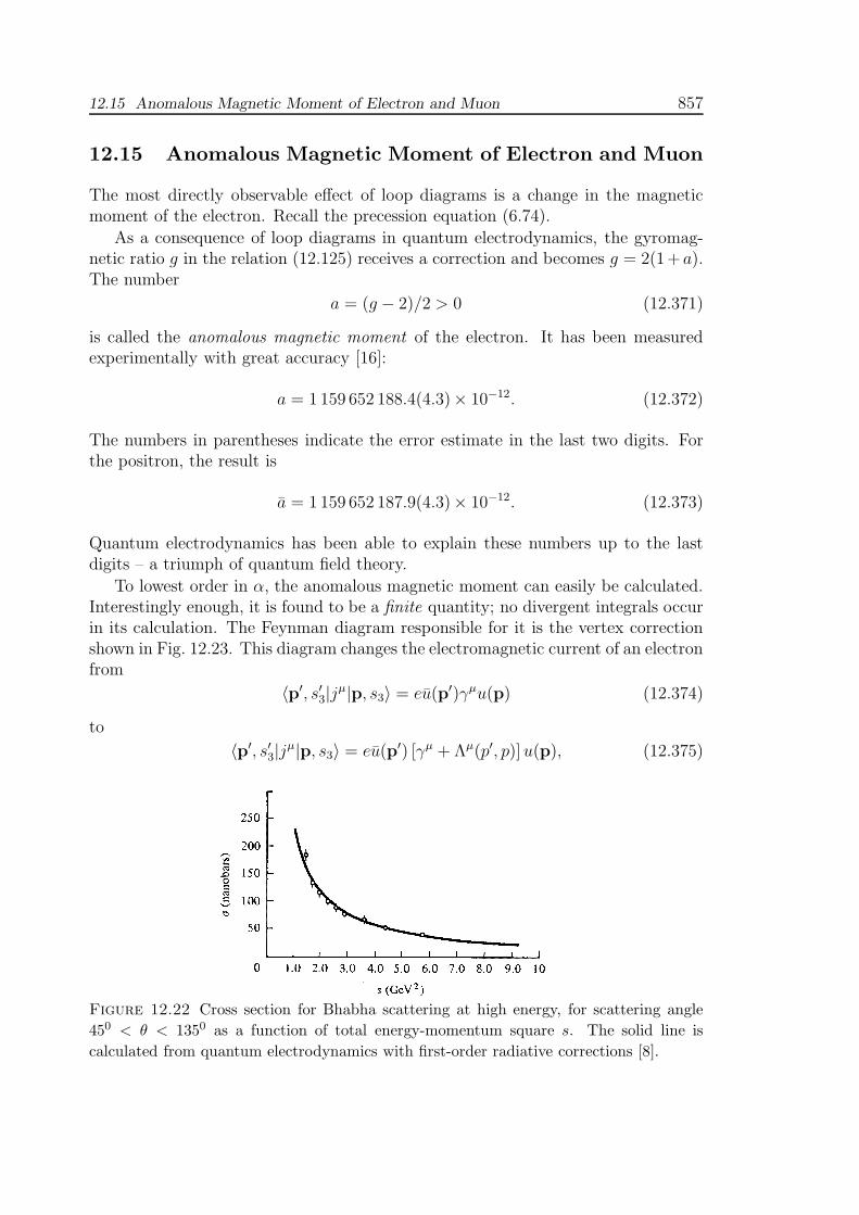
12.15 Anomalous Magnetic Moment of Electron and Muon 857
12.15 Anomalous Magnetic Moment of Electron and Muon
The most directly observable effect of loop diagrams is a change in the magneticmoment of the electron. Recall the precession equation (6.74).
As a consequence of loop diagrams in quantum electrodynamics, the gyromag-netic ratio g in the relation (12.125) receives a correction and becomes g = 2(1+a).The number
a = (g − 2)/2 > 0 (12.371)
is called the anomalous magnetic moment of the electron. It has been measuredexperimentally with great accuracy [16]:
a = 1 159 652 188.4(4.3)× 10−12. (12.372)
The numbers in parentheses indicate the error estimate in the last two digits. Forthe positron, the result is
a = 1 159 652 187.9(4.3)× 10−12. (12.373)
Quantum electrodynamics has been able to explain these numbers up to the lastdigits – a triumph of quantum field theory.
To lowest order in α, the anomalous magnetic moment can easily be calculated.Interestingly enough, it is found to be a finite quantity; no divergent integrals occurin its calculation. The Feynman diagram responsible for it is the vertex correctionshown in Fig. 12.23. This diagram changes the electromagnetic current of an electronfrom
〈p′, s′3|jµ|p, s3〉 = eu(p′)γµu(p) (12.374)
to
〈p′, s′3|jµ|p, s3〉 = eu(p′) [γµ + Λµ(p′, p)]u(p), (12.375)
Figure 12.22 Cross section for Bhabha scattering at high energy, for scattering angle
450 < θ < 1350 as a function of total energy-momentum square s. The solid line is
calculated from quantum electrodynamics with first-order radiative corrections [8].

858 12 Quantum Electrodynamics
Figure 12.23 Vertex correction responsible for the anomalous magnetic moment.
where the vertex correction Λµ(p′, p) is given by the Feynman integral
Λµ(p′, p) = −i4πα∫ d4k
(2π)4γν
1
/p′ + /k −Mγµ
1
/p + /k −Mγν
1
k2. (12.376)
This integral is logarithmically divergent at large momenta kµ. It can be regularizedby cutting the integration off at some large but finite momentum Λ which is laterremoved by a renormalization of the charge in the Lagrangian. There is also aninfrared divergence which is kept finite by cutting off the k-integration at a smallmass value k2 = µ2, much smaller than the electron mass, i.e., µ2 ≪M2.
To do the integral, we rewrite the integrand as
γν/p′ + /k +M
(p′ + k)−M2γµ
/p + /k +M
(p+ k)2 −M2γν
1
k2 − µ2, (12.377)
where we have introduced a small photon mass µ to avoid infrared divergencies atsmall momenta. We now collect the product of denominators into a single denomi-nator with the help of Feynman’s formula (11.158) for three denominators
1
ABC= 2
∫ 1
0dx∫ x
0dy[Ay +B(x− y) + C(1− x)]−3, (12.378)
so that
1
(p′ + k)−M2
1
(p+ k)2 −M2
1
k2(12.379)
= 2∫ 1
0dx∫ x
0dy[
(p′ + k)2−M2]
y +[
(p+k)2−M2]
(x−y) + (k2−µ2)(1− x)−3
.
This can be simplified to
2∫ 1
0dx∫ x
0dy
[k − p′y − p(x− y)]2 − µ2(1− x)−M2x2 + q2y(x− y)
−3.
(12.380)After performing a shift of the integration variable
k → k + p′y + p(x− y),
12.15 Anomalous Magnetic Moment of Electron and Muon 859
the vertex correction (12.376) takes the form
Λµ(p′, p) = −i4πα 2∫ 1
0dx∫ x
0dy∫
d4k
(2π)4(12.381)
×γν [/p′ (1− y)− /k − /p (x− y) +M ]γµ[/p (1− x− y)− /k − /p′ y +M ]
[k2 − µ2(1− x)−M2x2 + q2y(x− y)]3γν .
Instead of calculating this general expression, we shall restrict ourselves to matrix el-ements of the current between electron states and evaluate u(p′, s′3)Λ
µ(p′, p)u(p, s3).Then we can use the mass shell conditions p2 = p′2 = M2 and the Dirac equa-tions /p u(p, s3) = Mu(p, s3) and u(p′, s′3)/p = Mu(p′, s′3). We now employ ap-propriately the anticommutation rules of the gamma matrices using the formulas(12.220)–(12.222), perform a Wick rotation k0 → ik4, and integrate over the Eu-clidean four-momenta d4kE = 2π2dk k3, setting p2 = −p2E , p′2 = −p′E2. Cutting offthe k-integral at kE = Λ, we arrive at the triple integral
u(p′, s′3)Λµ(p′, p)u(p, s3)=α
∫ 1
0dx∫ x
0dy∫ Λ
0dkEk
3E
k3E[k2E + µ2(1−x)+M2x2+q2Ey(x−y)]
3
×u(p′, s′3)
γµ[
k2E − 2M2(x2 − 4x+ 2) + 2q2 (y(x− y) + 1− x)]
(12.382)
− 4Mp′µ(y − x+ xy)− 4Mpµ(x2 − xy − y)
u(p, s3).
The denominator is symmetric under the exchange y → x−y. Under this operation,the coefficients of pµ and p′µ are interchanged, showing that the vertex function issymmetric in pµ and p′µ. We can therefore replace each of these coefficients by thecommon average
y − x+ xy
x2 − xy − y
→ 1
2[(y − x+ xy) + (x2 − xy − y)] = − 1
2x(1 − x),
and rewrite (12.382) as
u(p′, s′3)Λµ(p′, p)u(p, s3)=α
∫ 1
0dx∫ x
0dy∫ Λ
µdkEk
3E
k3E[k2E+ µ2(1−x)+M2x2−q2y(x−y)]3
×u(p′, s′3)
γµ[
k2E − 2M2(x2 − 4x+ 2) + 2q2 (y(x− y) + 1− x)]
(12.383)
− 2M(p′µ + pµ)x(1− x) u(p, s3).
This expression may be decomposed as follows:
u(p′, s′3)Λµ(p′, p)u(p, s3) = u(p′, s′3)
[
γµH(q2)− 1
2M(p′µ + pµ)G(q2)
]
u(p, s3),
(12.384)
with the invariant functions
H(q2) =α
π
∫ 1
0dx∫ x
0dy∫ Λ
µdkE k
3E
k2E − 2M2(x2 − 4x+ 2) + 2q2[y(x− y) + 1− x]
[k2E + µ2(1− x) +M2x2 − q2y(x− y)]3
(12.385)

860 12 Quantum Electrodynamics
and
G(q2) =α
πM2
∫ 1
0dx∫ x
0dy∫ Λ
µdkE k
3E
4M2x(1− x)
[k2E + µ2(1− x) +M2x2 − q2y(x− y)]3 .
(12.386)
The momentum integral in the second invariant function G(q2) is convergentat small and large momenta, such that we can set the photon mass µ to zero andultraviolet to infinity. Using the integral formula
∫ ∞
0dk2E k
2E
1
(k2E +M21 )
3=
1
2M21
, (12.387)
we obtain
G(q2) =α
πM2
∫ 1
0dx∫ x
0dy
x(1− x)
M2x2 − q2y(x− y). (12.388)
The integral over y yields
G(q2) =α
πM2
∫ 1
0dx 4(1− x)
1√
q2(4M2 − q2)arctan
√
q2
4M2 − q2, (12.389)
leading to
G(q2) =α
π
2M2
√
q2(4M2 − q2)arctan
√
q2
4M2 − q2, (12.390)
which can be rewritten as
G(q2) =α
2π
2θ
sin 2θ, with sin2 θ ≡ q2
4M2. (12.391)
For small q2, it has the expansion
G(q2) =α
2π
(
1 +q2
6M2+ . . .
)
. (12.392)
In the first invariant function H(q2), both the cutoff and the photon mass arenecessary to obtain a finite result. The divergence can be isolated by a subtractionof the integrand, separating
H(q2) = H(0) + ∆H(q2), (12.393)
with a divergent integral
H(0) =α
π
∫ 1
0dx∫ x
0dy∫ ∞
0dkE k
3E
k2E − 2M2(x2−4x+2)
[k2E + µ2(1−x) +M2x2]3
(12.394)

12.15 Anomalous Magnetic Moment of Electron and Muon 861
and a convergent one at large momenta
∆H(q2) =α
π
∫ 1
0dx∫ x
0dy∫ ∞
0dkE k
3E
k2E − 2M2(x2−4x+2) + 2q2[y(x−y) + 1− x]
[k2E + µ2(1−x) +M2x2− q2y(x−y)]3
− k2E − 2M2(x2 − 4x+ 2)
[k2E + µ2(1−x) +M2x2]3
. (12.395)
The divergent momentum integral in (12.394) must be performed with the help ofsome regularization scheme, for which we choose the Pauli-Villars regularization,replacing the photon propagator as follows:
1
k2 − µ2→ 1
k2 − µ2− 1
k2 − Λ2, (12.396)
where Λ is a large cutoff mass. Then we may use the formula∫ ∞
0dk2E k
2E
[
k2E +M22
(k2E + µ2(1− x) +M21 )
3
]
− [µ2 → Λ2]
= − logµ2(1− x) +M2
1
Λ2(1− x)+
1
2
M22
µ2(1− x) +M21
. (12.397)
With this, the convergent momentum integral (12.395) yields
∆H(q2) =α
2π
∫ 1
0dx∫ x
0dy
−M2(x2 − 4x+ 2)− q2[y(x− y) + 1− x]
µ2(1− x) +M2x2 − q2y(x− y)
+M2(x2 − 4x+ 2)
µ2(1− x) +M2x2− log
[
µ2(1− x) +M2x2 − q2y(x− y)
µ2(1− x) +M2x2
]
. (12.398)
If the photon mass is set equal to zero, the integral is divergent at x = 0. Thephysical meaning of this infrared divergence will be explained later.
Let us first understand ∆H(q2) for small q2 by expanding ∆H(q2) = ∆H ′(0)q2+O(q4). Then ∆H ′(0) is given by the integral
∆H ′(0) =α
2π
∫ 1
0dx∫ x
0dy
y(x− y) + 1− x
µ2(1− x) +M2x2
− M2(x2 − 4x+ 2)y(x− y)
[µ2(1− x) +M2x2]2+
y(x− y)
µ2(1− x) +M2x2
=α
2π
(
1
3log
M2
µ2− 1
12
)
, (12.399)
where we have discarded all terms which go to zero for µ→ 0.The full result is
H(q2) = H(0) +α
2π
[(
logM2
µ2− 2
)(
1− 2θ
tan 2θ
)
+ θ tan θ +4
tan 2θ
∫ θ
0dx x tanx+
2θ
sin 2θ
]
, (12.400)
which has precisely the first Taylor coefficient (12.399).

862 12 Quantum Electrodynamics
12.15.1 Form Factors
We now introduce the customary Lorentz-invariant decompositions of the matrixelements of the current (12.375) of a spin-1/2 particle as follows:
〈p′|jµ|p〉 = eu(p′)[
γµF (q2) +i
2MσµνqνG(q
2)]
u(p′). (12.401)
The invariant functions F (q2) and G(q2) are the standard form factors of the elec-tron. The relation between this and (12.384) follows directly from Gordon’s decom-position formula (12.141), showing that G(q2) in (12.386) coincides with G(q2) in(12.401), whereas
F (q2) = 1 +H(q2)−G(q2). (12.402)
The charge form factor F (q2) at q2 = 0 specifies the charge of the electron.Inserting (12.400), we obtain
F (q2) = F (0) +α
2π
[(
logM2
µ2− 2
)(
1− 2θ
tan 2θ
)
+ θ tan θ +4
tan 2θ
∫ θ
0dx x tanx
]
, (12.403)
where
F (0) ≡ 1 +α
2π
(
logΛ
M+
9
4− log
M2
µ2
)
. (12.404)
The value F (0) contains both the ultraviolet and the infrared cutoff. The subtractedfunction ∆F (q2) ≡ F (q2) − F (0) has only an infrared divergence. In writing downthe expressions (12.403) and (12.404), we have ignored all contributions which vanishfor µ→ 0 and Λ → ∞.
Due to the loop integral, the charge is changed to the new value
e1 = eF (0) = e
[
1 +α
2π
(
logΛ
M+
9
4− 2 log
M
µ
)]
. (12.405)
The factor is commonly denoted as the renormalization constant Z−11 . To order α,
it is
Z1 ≡ F−1(0) = 1− α
2π
(
logΛ
M+
9
4− 2 log
M
µ
)
. (12.406)
According to the theory of renormalization, this has to be equated with the exper-imentally observed charge. After this we can replace, in Eq. (12.403), the numberF (0) by 1, and the bare fine-structure constant α by the physical one (keeping thenotation, for simplicity). The latter substitution is also done in G(q).

12.15 Anomalous Magnetic Moment of Electron and Muon 863
12.15.2 Charge Radius
For small momentum transfers q2, the renormalized charge form factor has the Taylorseries expansion
FR(q2) = 1 + q2
α
3πM2
(
logM
µ− 3
8
)
+O(q4). (12.407)
The form factor of the anomalous magnetic moment is, for small q,
GR(q2) = q2
α
3πM2
1
4+O(q4). (12.408)
Due to the emission and absorption of virtual photons, the electron is shakenover a finite range. It is customary to define here a charge radius Re of the electronby the first term in the expansion of the charge form factor2
F (q2) = 1− q2R2e
6+ . . . . (12.409)
The factor 1/6 is due to the fact that for a uniformly charged shell of radius Re, theFourier transform of the charge density has the expansion
F (q2) =∫
d3x eiqxρ(x) =∫
d3x[
1 + iqx− 1
2(qx)2 + . . .
]
ρ(x)
= 1− 1
6q2∫
d3x r2ρ(x) = 1− q2R2e
6+ . . . . (12.410)
Setting q0 = 0 in Eq. (12.407), we find that due to the vertex correction, the chargeradius Rvc
e of the electron is given by
R2evc =
α
π
2
M2
(
logM
µ− 3
8
)
. (12.411)
If the zeroth component of the current (12.401) couples to a static electric po-tential A0(x), the q
2-term in (12.407) yields a correction factor
[
1 +R2e
6∇
2
]
A0(x). (12.412)
The fluctuations of the electron position leads to an extra term proportional tothe harmonic average of the potential. Since the potential obeys Gauss’ law, thisis nonzero only where there are charges. In an atom of nuclear charge Ze at theorigin, the potential is
eA0(x) = VC(x) = −Zαr
(12.413)
2Note the difference of this quantity with respect to the classical electron radius (12.234).

864 12 Quantum Electrodynamics
and the harmonic average produces an additional δ-function at the origin:
e∇2A0(x) = 4πZα δ(3)(x). (12.414)
Thus the correction factor changes the Coulomb potential into an effective potential
V effC = −Zα
r+R2evc
6Zα 4πδ(3)(x). (12.415)
The prediction of this additional term is the origin of one of the early triumphsof QED. The δ-function leads to an energy shift of s-wave orbits with respect tothose of nonzero orbital angular momentum, called the Lamb shift . It removes thedegeneracy between the 2S1/2 and the 2P1/2 predicted by Dirac’s equation in anexternal Coulomb field. It will be discussed in detail below.
12.15.3 Anomalous Magnetic Moment
On the right-hand side of the current matrix element (12.401) we replace the γµ-term by a combination of vectors p′µ + pµ and σµνqν , as before in (12.141), and seethat the magnetic moment of the free electron acquires a correction factor 1+G(0).Thus the gyromagnetic ratio g in Eq. (12.126) is changes from g = 2 to
g ≡ 2(1 + a) = 2[1 +G(0) + . . . ] (12.416)
[recall (12.371)]. The number G(0) yields therefore directly the anomalous magneticmoment:
a = G(0). (12.417)
In contrast to the charge, this quantity is finite. Its value is [17]
a = G(0) =α
2π∼ 1 161 409 74292× 10−12. (12.418)
This result was first calculated by Schwinger [18]. It is about 1.5% larger thanthe experimental values (12.372) and (12.373). The difference can be explained byhigher-order electrodynamic and strong-interaction corrections [19]. By includingall diagrams of sixth order in perturbation theory one finds, after a considerableeffort (there are 72 Feynman diagrams to sixth order), the expansion
a =α
2π+ c2
(
α
π
)2
+ c3
(
α
π
)3
(12.419)
with the coefficients [20]
c2 =197
144+(
1
2− 3 log 2
)
ζ(2) +3
4ζ(4) = −0.328 478 965 . . . , r (12.420)
c3 = 1.176 11(42). (12.421)

12.15 Anomalous Magnetic Moment of Electron and Muon 865
Up to c2, the theory is lower than the experimental number by only 1 part in 105.Adding the c3-term, the theoretical value becomes
a = 1 159 652 140.4(27.1)× 10−12, (12.422)
reducing the discrepancy to 1 part in 108. The error is mainly due to the uncertaintyin the fine-structure constant [17].
The above calculation may be used to show that the anomalous magnetic momentof an antiparticle is the same as for a particle. The matrix element of the initialcurrent between positron states is
〈p′, s′3|jµ(x)|p, s3〉 = e〈0|b(p′, s′3)ψ(x)γµψ(x)b†(p, s3)|0〉 = −ev(p′, s3)γ
µu(p, s3)eiqx,
(12.423)rather than (12.129). The minus sign is due to the odd number of exchanges offield operators necessary to evaluate the anticommutators. If both momenta arezero, only the zeroth component survives, showing that the charge of the positronis −e. For small momentum transfers, we calculate the second spatial componentof (12.423) more explicitly as
〈p′, s′3|j2(x)|p, s3〉 = −ev(0, s3)γ2eiζ1(iγ0γ1)/2v(0, s3), (12.424)
and compare this with (12.134). The linear term in ζ1 contains the contributionof the charge form factor to the magnetic moment. We see that (12.424) has theopposite overall sign of (12.134) which is compensated by an opposite sign in theexponent of the Lorentz transformation. Thus we obtain the matrix element of j2
between positrons:−ieζ1v(0, s3)S3v(0, s3) = ieζ1s3, (12.425)
with an opposite sign in comparison with the electron in (12.135). The sign change atthe end is caused by the opposite spin orientation of the two-spinors ξ(s3) containedin the spinors v(0, s3) [recall (4.684),(4.685) and (4.676)].
An opposite sign is also found for the contribution from the second form factorwhere the matrix element of the electron is
eu(0, s3)i
2Mσ21q1G(0)u(0, s3) = −ieu(0, s3)S3ζ
1G(0)u(0, s3) = −ieζ1s3G(0).(12.426)
This produces the correction to the g-factor
g = 2[1 +G(0)]. (12.427)
For a positron, the matrix element of the current is
−ev(p′, s′3)[γ2F (q2) +
i
2Mσ2νqνG(q
2)]v(p, s3), (12.428)
and the second term becomes, for p′ = 0 and small p in the x-direction,
−ev(0, s3)i
2Mσ21q1G(0)v(0, s3) = iev(0, s3)S3ζ
1G(0)v(0, s3) = ieζ1s3G(0),
(12.429)
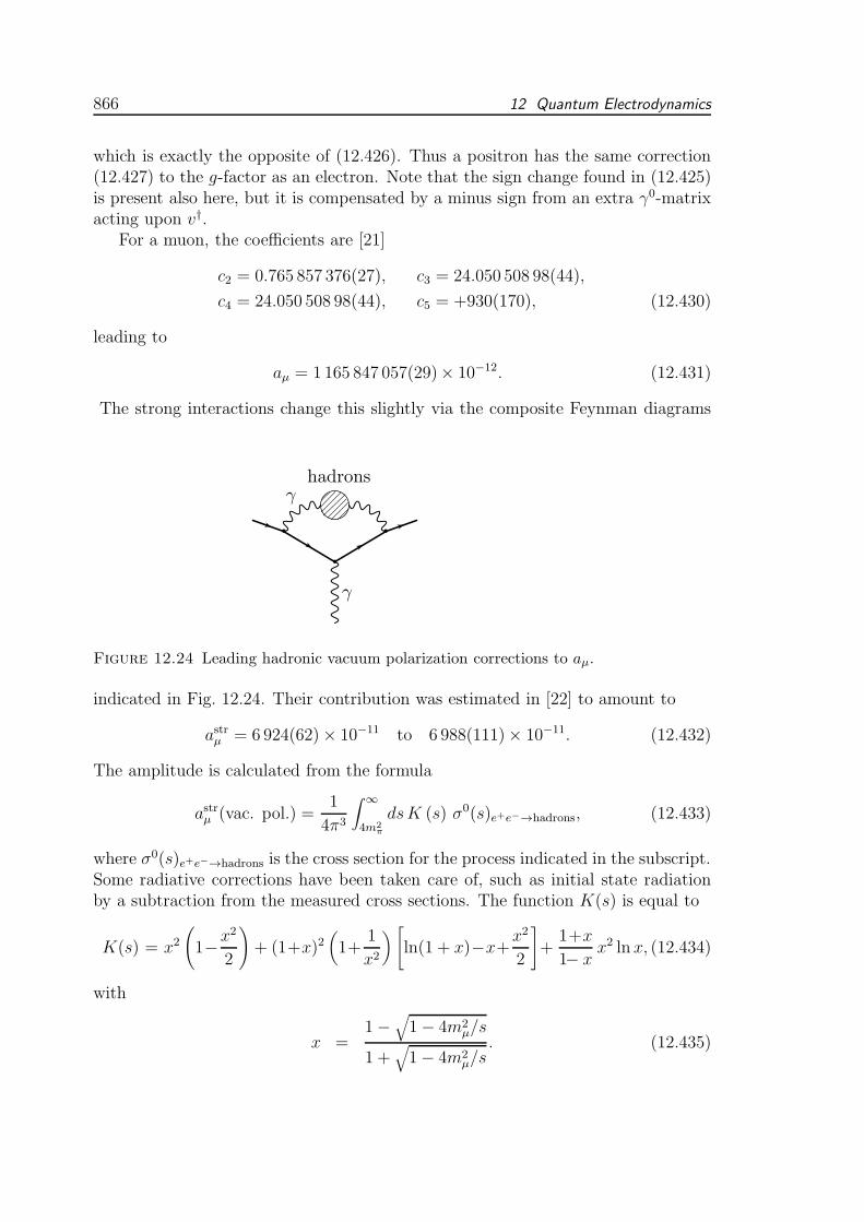
866 12 Quantum Electrodynamics
which is exactly the opposite of (12.426). Thus a positron has the same correction(12.427) to the g-factor as an electron. Note that the sign change found in (12.425)is present also here, but it is compensated by a minus sign from an extra γ0-matrixacting upon v†.
For a muon, the coefficients are [21]
c2 = 0.765 857 376(27), c3 = 24.050 508 98(44),
c4 = 24.050 508 98(44), c5 = +930(170), (12.430)
leading to
aµ = 1 165 847 057(29)× 10−12. (12.431)
The strong interactions change this slightly via the composite Feynman diagrams
hadronsγ
γ
Figure 12.24 Leading hadronic vacuum polarization corrections to aµ.
indicated in Fig. 12.24. Their contribution was estimated in [22] to amount to
astrµ = 6 924(62)× 10−11 to 6 988(111)× 10−11. (12.432)
The amplitude is calculated from the formula
astrµ (vac. pol.) =1
4π3
∫ ∞
4m2π
dsK (s) σ0(s)e+e−→hadrons, (12.433)
where σ0(s)e+e−→hadrons is the cross section for the process indicated in the subscript.Some radiative corrections have been taken care of, such as initial state radiationby a subtraction from the measured cross sections. The function K(s) is equal to
K(s) = x2(
1−x2
2
)
+ (1+x)2(
1+1
x2
)
[
ln(1 + x)−x+x2
2
]
+1+x
1− xx2 ln x, (12.434)
with
x =1−
√
1− 4m2µ/s
1 +√
1− 4m2µ/s
. (12.435)

12.15 Anomalous Magnetic Moment of Electron and Muon 867
√s (GeV) astrµ (vac. pol.)× 1011
2mπ − 1.8 6343± 601.8− 3.7 338.7± 4.63.7− 5 + ψ(1S, 2S) 143.1± 5.45− 9.3 68.7± 1.19.3− 12 12.1± 0.512−∞ 18.0± 0.1
Total 6924± 62
Table 12.1 Different contributions to astrµ (vac. pol.) in the integral 12.433.
It comes from the remaining part of the diagram. The contributions from thedifferent parts of the cross sections to astrµ (vac. pol.) in the integral (12.433) areseparately listed in Table 12.15.3. The weak interactions in the standard model addto this [23]
aEWµ (1 loop) =5
3
Gµm2µ
8√2π2
[
1 +1
5(1− 4 sin2 θW )2 +O
(
m2µ
M2
)]
≈ 195× 10−11, (12.436)
whereGµ = 1.16637(1)×10−5 GeV−2, sin2 θW ≡ 1−M2W /M
2Z ≃ 0.223. andM =MW
or MHiggs. See Fig. 12.25 for the Feynman diagrams.
g
W W
Z
g
H
g
(a) (b) (c)
Figure 12.25 One-loop electroweak radiative corrections to aµ. The wiggly lines are
gluons.
Two-loop corrections change this slightly by
aweakµ (2 loop) = −43(4)× 10−11, (12.437)
if we assume a Higgs particle mass of mH ≃ 150 GeV (with little sensitivity to theexact value). Altogether, we obtain
atheoryµ = 1 165 915 97(67)× 10−11, (12.438)
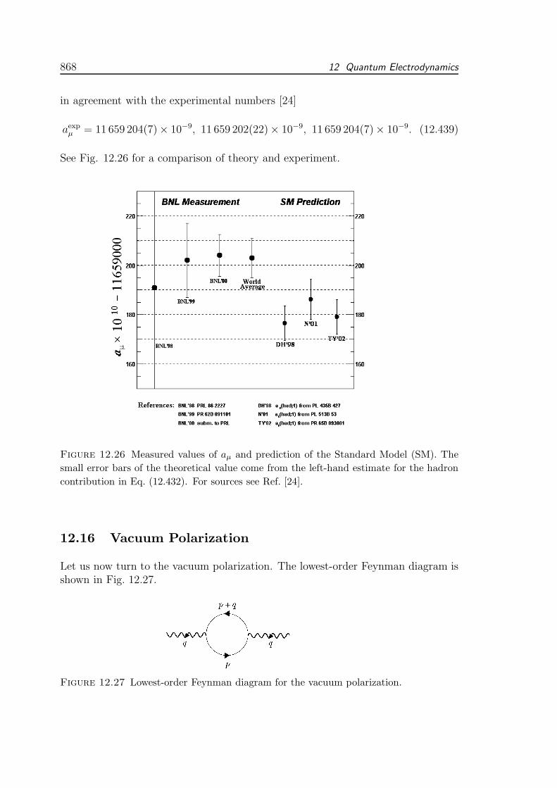
868 12 Quantum Electrodynamics
in agreement with the experimental numbers [24]
aexpµ = 11 659 204(7)× 10−9, 11 659 202(22)× 10−9, 11 659 204(7)× 10−9. (12.439)
See Fig. 12.26 for a comparison of theory and experiment.
Figure 12.26 Measured values of aµ and prediction of the Standard Model (SM). The
small error bars of the theoretical value come from the left-hand estimate for the hadron
contribution in Eq. (12.432). For sources see Ref. [24].
12.16 Vacuum Polarization
Let us now turn to the vacuum polarization. The lowest-order Feynman diagram isshown in Fig. 12.27.
Figure 12.27 Lowest-order Feynman diagram for the vacuum polarization.

12.16 Vacuum Polarization 869
In general, the propagator of the photon has the form
Gµν(q) = iP µν(q)
q2, (12.440)
where the polarization tensor P µν(q) depends on the gauge [see (12.111)]. From thelowest-order Feynman diagram in Fig. 12.27, the propagator receives a lowest-ordercorrection
Gµν0 (q) [−iΠλκ(q)]G
κν0 (q), (12.441)
where −Πµν(k) is given by the Feynman integral.
−iΠµν(q) = e2∫
d4p
(2π)4tr[γµ(/p + /q +M)γν(/p +M)]
[(p+ q)2 −M2](p2 −M2). (12.442)
Using Feynman’s formula (11.156)
1
AB=∫ 1
0dz
1
[Az +B(1− z)]2, (12.443)
we rewrite (12.442) as
−iΠµν(q) = e2∫ 1
0dz∫ d4p
(2π)4tr[γµ(/p + /q +M)γν(/p +M)]
[(p+ qz)2 + q2(z − z2)−M2]2. (12.444)
This expression is symmetric in µ and ν. A shift in the p-integration by an amountqz brings it to the form
−iΠµν(q) = e2∫ 1
0dz∫ d4p
(2π)4trγµ[/p + /q (1− z) +M ]γν(/p − /q z +M)
[p2 + q2(z − z2)−M2]2. (12.445)
After evaluating the trace, dropping odd terms in p, and using the symmetry in µand ν, we obtain
−iΠµν(q) = 4e2∫ 1
0dz∫ d4p
(2π)4−(−gµνq2 + 2qνqν)(z − z2)−gµν(p2−M2)+2pµpν
[p2 + q2(z − z2)−M2]2.
(12.446)Because of the rotational symmetry of the integrand we can use the first replacementrule in Eq. (11.136) to replace −gµν(p2 −M2) + 2pµpν by −gµν(p2/2−M2).
The momentum integral is quadratically divergent, since there are two morepowers of integration variables in the numerator than in the denominator. Thesituation is improved by imposing the requirement of gauge invariance, qµΠµν(q) =0. This makes the final results independent of the gauge choice in the photonpropagator. Thus we postulate, for the moment, the vanishing of the divergentintegral
−iqµΠµν(q) = e2qν 4∫ 1
0dz∫
d4p
(2π)4−q2(z − z2)− (p2/2−M2)
[p2 + q2(z − z2)−M2]2. (12.447)

870 12 Quantum Electrodynamics
We shall verify in the next Subsection that this is guaranteed if we calculate theFeynman diagrams by analytic regularization in D dimensions rather than D = 4.
Thus we are left with the logarithmically divergent integral
−iΠµν(q) = −(−gµνq2 + qµqν) 8e2∫ 1
0dz(z − z2)
∫
d4p
(2π)41
[p2 + q2(z − z2)−M2]2.
(12.448)Let us define the invariant function that accompanies the tensor (−gµνq2 + qµqν) =q2Pµν(q) as −iΠ(q2), i.e., we write
−iΠµν(q) ≡ −iPµν(q)q2Π(q2). (12.449)
If we expandΠ(q2) = Π(0) + Π′(0)q2 + . . . , (12.450)
we see that only Π(0) is logarithmically divergent:
−iΠ(0) = −8e2∫ 1
0dz(z − z2)
∫ d4p
(2π)41
(p2 −M2)2, (12.451)
whereas all remaining terms in the expansion (12.450) are finite, for example thefirst term:
−iΠ′(0) = 16e2∫ 1
0dz(z − z2)2
∫
d4p
(2π)41
(p2 −M2)3. (12.452)
Since the mass M carries a small negative imaginary part, we now perform a Wickrotation of the integration contour, setting p0 = ip4 and letting p4 run from −∞ to∞. Thus we substitute p2 = −p2E and d4p/(2π)4 = id4pE/(2π)
4, and calculate from(12.452):
Π′(0) =e2
(2π)44
15
π2
M2=
α
6πM2
1
5. (12.453)
In the divergent quantity Π(0), we perform a Wick rotation so that the integrald4p/(2π)4 turns into an integral over all Euclidean four-momenta d4pE/(2π)
4 =S4dpEp
3E = dp2E p
2E/16π
2. If we introduce an ultraviolet momentum cutoff at Λ2, weobtain
Π(0) = 8e21
6
∫
d4pE(2π)4
1
(p2E +M2)2= 8e2
1
6
1
16π2
∫ ∞
0dp2E
p2E(p2E +M2)2
=α
π
1
3
(
logΛ2
M2− 1
)
. (12.454)
The complete invariant function of the polarization tensor is therefore
Π(q2) =α
π
[
1
3
(
logΛ2
M2− 1
)
+(
2
3+
1
3 sin2 θ
)
(
1− θ
tan θ
)
− 1
9
]
. (12.455)

12.16 Vacuum Polarization 871
For small q2, we expand
Π(q2) =(
2
3+
1
3 sin2 θ
)
(
1− θ
tan θ
)
=1
9+
4
15θ2 + . . . , (12.456)
and find the bracket to behave like
Π(0) + Π′(0)q2 + . . . =α
π
[
1
3
(
logΛ2
M2− 1
)
+1
15
q2
M2+O(q4)
]
. (12.457)
The last term agrees with the result (12.453) of a direct calculation of Π′(0). Itis gratifying to find out that the condition (12.447) is fulfilled by the dimensionalregularization in d = 4− ǫ dimensions.
Note that the expression (12.455) is real only for q2 < M2. When q2 > (2M)2 theexternal field can produce electron-positron pairs and Π(q2) acquires an imaginarypart. The imaginary part causes a decrease of the probability amplitude for theoccurrence of a pure scattering process below the threshold of pair production.
A string of vacuum polarization diagrams produces the geometric series
Gµν = Gµν0 +Gµλ
0 [−iΠλκ]Gκν0 + . . .+Gµλ
0 [−iΠλκ]Gκσ0 [−iΠστ ]G
τν0 + . . . , (12.458)
which can be summed up to
Gµν(q) = [G−1µν (q) + iΠµν(q)]
−1−1. (12.459)
Inserting the tensor decomposition (12.449), this can be written as
Gµν(q) = iP µν(q)
q2[1− Π(q2)]≈ i
P µν(q)
q2[1 + Π(0) + Π′(0)q2 − . . .](12.460)
For small q2, the photon propagator is, therefore,
Gµν(q) ≈ iPµν(q)
q2
1 + Π(0) +α
15πM2q2−1
. (12.461)
The divergent number 1+Π(0) can be absorbed into the field renormalization factor,after defining
AµR(x) = Z−1/23 A(x) (12.462)
with
Z3 = [1 + Π(0)]−1 = 1− α
3πlog
Λ2
m2+ . . . . (12.463)
This corresponds to renormalizing the charge to
αR = Z3α. (12.464)
The propagator of the renormalized field AµR is then
GµνR (q) = i
Pµν(q)
q2
(
1 +αR15π
q2
M2
)−1
. (12.465)
872 12 Quantum Electrodynamics
For a given static source of charge Ze at the origin, the Coulomb potential
VC(x) = −Zαr
(12.466)
is obtained by applying the free propagator Gµν0 to the current jµ(x) = δµ0 Zeδ
(3)(x).To lowest order in α, the vacuum polarization changes G0
µν(q) by a factor(
1− αR15π
q2
M2
)
which is equivalent to multiplying the potential VC(x) by a factor(
1− αR15π
∇2
M2
)
.
The potential is therefore modified to
V RC (x) = −Zα
[
1
r+
α
15πM24πδ(3)(x)
]
. (12.467)
A comparison with (12.407)–(12.415) shows that the vacuum polarization decreasesthe effective radius of the electron (12.411), derived from the vertex correction, by
R2evp = − α
3πM2
1
5, (12.468)
thus giving rise to a total effective radius determined to lowest order in α by:
R2evp = − α
3πM2
1
5
(
logM
µ− 3
8− 1
5
)
. (12.469)
Since the finite radius of the electron gives rise to the Lamb shift to be derivedbelow, the vacuum polarization decreases the Lamb shift.
12.17 Dimensional Regularization
We still must show that the divergent integral (12.447) is really zero, to ensure thegauge invariance of the self-energy (12.446). In D dimensions, the Dirac matriceshave the dimension 2D/2, and (12.446) reads [26]
−iΠµν(q) = 2D/2e2∫ 1
0dz∫
dDp
(2π)D−(−gµνq2+2qνqν)(z−z2)−gµν(p2−M2)+2pµpν
[p2 + q2(z − z2)−M2]2.
(12.470)Then the previous replacement under the integral pµpν → gµν/4 becomes pµpν →gµν/D [recall (11.136)]. The integral dDp over all four-momenta may now be Wick-rotated to
i∫
dDpE/(2π)D = iSD/2(2π)
D∫ ∞
0dp2E(p
2E)
D/2−1, (12.471)

12.18 Two-Dimensional QED 873
where SD is the surface of the unit sphere (11.126). Hence we can rewrite the integral(12.447) in Euclidean spacetime as
−iqµΠµν(q) = e2qν 2D/2i
∫ 1
0dz∫
dDpE(2π)D
−q2(z−z2)+ (1− 2/D)p2E +M2
[p2E +m2]2, (12.472)
where
m2 = m2(q2, z) ≡M2 − q2z(1− z), (12.473)
and further as
−iqµΠµν(q) = e2qν 2D/2i
∫ 1
0dz∫ dDpE
(2π)D2m2/D + (1− 2/D)(p2E +m2)
[p2E +m2]2. (12.474)
Now we use Formula (11.130) to replace
∫
dDpE(2π)D
1
(p2E +m2)ν= SD
Γ(D/2)Γ (ν −D/2)
2Γ(ν)[m2]D/2−ν , (12.475)
so that
−iqµΠµν(q)=e2qν 2
D/2iSDΓ(D/2)
2
×[
2
DΓ (1−D/2)Γ(2) +
(
1− 2
D
)
Γ (2−D/2)Γ(1)]∫ 1
0dz[m2]D/2−1 = 0, (12.476)
thus guaranteeing the gauge invariance of the vacuum polarization tensor in anydimension D [10].
12.18 Two-Dimensional QED
If the bare electron mass is zero, an interesting phenomenon arises in two dimensions:The self-energy of the photon makes the photon massive. This happens in spite ofgauge invariance of the Lagrangian, as pointed out by Schwinger [6] in 1962. Sincethis was a surprise, the two-dimensional massless QED is called the Schwinger model
[27].Consider the self-energy (12.448) in D spacetime dimensions where the prefactor
4 in Eq. (12.446) is replaced by 2D/2, so that (12.448) reads
−iΠµν(q)=−(−gµνq2 + qµqν) 2D/2+1e2
∫ 1
0dz(z−z2)
∫
dDp
(2π)D1
[p2 + q2(z−z2)−M2]2.
(12.477)Here the integral over dDp in momentum spacetime is Wick-rotated, as in (12.471),into the Euclidean momentum integral
SD2(2π)D
i∫ ∞
0dp2E
1
(p2E +m2)2=
SD2(2π)D
i[m2]D/2−2Γ(D/2)Γ(2−D/2)Γ(2)
, (12.478)

874 12 Quantum Electrodynamics
withm2 determined by Eq. (12.473). Inserting this into (12.477) yields, for−iΠµν(q)of massless electrons, the tensor
−(−gµνq2+qµqν) 2D/2+1e2i∫ 1
0dz[z(1−z)]D/2−1(−q2)D/2−2 SD
2(2π)DΓ(D/2)Γ(2−D/2)
Γ(2),
(12.479)which is equal to3
−(−gµνq2 + qµqν)2D/2+1e2i
Γ2(D/2)
Γ(D)(−q2)D/2−2 SD
2(2π)DΓ(D/2)Γ(2−D/2)
Γ(2), (12.480)
so that we obtain, in D = 2 dimensions,
−iΠµν(q)=−i(−gµνq2 + qµqν)4e2
−q2S2
2(2π)2=−i(−gµνq2 + qµqν)
e2
−πq2 =−iPµνe2
−πq2 ,(12.481)
or, recalling (12.449),
!Π(q) = − e2
πq2. (12.482)
Inserting this into (12.460), we obtain the renormalized photon propagator
Gµν(q) = iP µν(q)
q2 + q2Π(q)= i
P µν(q)
q2 − e2/π. (12.483)
This shows that the photon has acquired a nonzero mass m2γ = e2/π. The effective
Lagrangian of the photon to this order is
Leff = − 1
4F µν(1 +m2
γ/ )Fµν . (12.484)
The Schwinger model illustrates the remarkable fact that in spite of the gauge invari-ance of the theory, a mass term can be generated for the photon by a loop diagramof a massless fermion.
12.19 Self-Energy of Electron
The lowest-order Feynman diagram for the self-energy of the electron is shown inFig. 12.28. It adds to the electron propagator a term
G0(p)[−iΣ(p)]G0(p), (12.485)
where
G0(p) =i
/p −M(12.486)
3I.S. Gradshteyn and I.M. Ryzhik, Table of Integrals, Series, and Products , Academic Press,New York, 1980, Formula 3.191.3.

12.19 Self-Energy of Electron 875
Figure 12.28 Lowest-order Feynman diagram for the self-energy of the electron.
is the free Dirac propagator and the self-energy −iΣ(p) of the electron is given bythe diagram in Fig. 12.28. Explicitly:
−iΣ(p) = e2∫
d4k
(2π)4γµ
/p − /k +M
(p− k)2 −M2γµ
1
k2. (12.487)
Using the anticommutation rule (12.214), we can simplify, in the numerator,
γµ(/p − /k +M)γµ = −2(/p − /k ). (12.488)
The integral is logarithmically divergent at large k. It also has an infrared diver-gence. To enforce convergence, we employ the Pauli-Villars regularization methodand modify the photon propagator as follows:
1
k2→ 1
k2 − µ2− 1
k2 − Λ2, (12.489)
where Λ is a large cutoff mass and µ is a small photon mass. The self-energy becomes
−iΣ(p) = e2∫
d4k
(2π)4−2(/p − /k ) + 4M
(p− k)2 −M2
(
1
k2 − µ2− 1
k2 − Λ2
)
. (12.490)
The mass parameter Λ cuts off the contribution of short-wave photons with k ≫ Λ2.At the end we shall take the cutoff to infinity.
By adding the same Feynman diagram repeatedly to an electron line, we obtainthe geometric series
G0(p) +G0(p)[−iΣ(p)]G0(p) +G0(p)[−iΣ(p)]G0(p)[−iΣ(p)]G0(p) + . . . , (12.491)
which can be summed up to
G(p) =i
/p −M − Σ(p). (12.492)
Using Feynman’s formula (12.443), this can be rewritten as
Σ(p) = −ie2∫ 1
0dx∫
d4k
(2π)4
×
−2(/p − /k ) + 4M
[−(k − px)2 − p2x(1− x) +M2x+ Λ2(1− x)]2− (Λ = µ)
. (12.493)

876 12 Quantum Electrodynamics
A simplification occurs by shifting the integration variable from k to k + px. Thenthe terms proportional to k are off in k and can be dropped. After performing aWick rotation of the integration contour, we obtain
Σ(p)=2π2e2
(2π)4
∫ 1
0ds∫ 1
0dkEk
3E
−2/p (1− x) + 4M
[k2E − p2x(1 − x) +M2x+ Λ2(1− x)]2−(Λ=0)
.
(12.494)The kE-integral is easily done, and yields
Σ(p) =π2e2
(2π)4
∫ 1
0dx [−2/p (1− x) + 4M ]
×
log
[
−p2x(1− x) +M2x+ Λ2(1− x)
−p2x(1 − x) +M2x
]
− (Λ = µ)
. (12.495)
The right-hand side is a 4×4-matrix in spinor space which may be decomposed intoinvariant functions
Σ(p) = (/p −M)A(p2) +B(p2), (12.496)
where
A(p2) =π2e2
(2π)4
∫ 1
0dx[−2(1− x)]
log f(p2, x,Λ)− (Λ = µ)
,
B(p2) =π2e2
(2π)4
∫ 1
0dx 2M(1 + x)
log f(p2, x,Λ)− (Λ = µ)
, (12.497)
with
f(p2, x,Λ) =−p2x(1 − x) +M2x+ Λ2(1− x)
−p2x(1− x) +M2x. (12.498)
The invariant functions are logarithmically divergent for large Λ.We may expand them around the mass shell p2 = M2 in powers of p2 −M2.
Then only the lowest expansion terms carry the logarithmic divergence:
A(M2) =π2e2
(2π)4
∫ 1
0dx [−2(1− x)] log
[
M2x2 + Λ2(1− x)
M2x2
]
,
B(M2) =π2e2
(2π)4
∫ 1
0dx 2M(1 + x) log
[
M2x2 + Λ2(1− x)
M2x2
]
,
B′(M2) =π2e2
(2π)4
∫ 1
0dx 2M(1 + x)(1− x)
×[
Λ2(1− x)
M2x[M2x2 + Λ2(1− x)]− µ2(1− x)
M2x[M2x2 + µ2(1− x)]
]
. (12.499)
All higher expansion terms are finite and can be evaluated with an infinite cutoffΛ. We have also dropped all terms that vanish in the limit of zero photon mass µ.Omitting the regular parts of the self-energy, the propagator becomes
G(p) =i
(/p −M)[1 + A(M2)] +B(M2) +B′(M2)(p2 −M2)

12.20 Ward-Takahashi Identity 877
=1
1 + A(M2) + 2MB′(M2)
i
/p −M − δM, (12.500)
where
δM ≡ − B(M2)
1 + A(M2) + 2MB′(M2). (12.501)
The prefactor in the denominator is commonly denoted by
Z2 ≡ 1 + A(M2) + 2MB′(M2). (12.502)
It can be removed by renormalizing the field ψ(x) to ψR(x) = Z1/22 ψ(x). The
renormalized field has then a propagator with a pole term i/(/p −M). For large Λ2,we can simplify the results for Z2 and δM2 to order α:
Z2 − 1=− α
2π
∫ 1
0dx
(1−x)[
logΛ2
M2+log
1−xx2
]
−21−x2x
[
1− µ2(1−x)M2x2 + µ2(1−x)
]
,
δM2 =α
2π
∫ 1
0dx(1+x)
[
logΛ2
M2+ log
1−xx2
]
. (12.503)
Performing the integrals over x yields
Z2 − 1 = − α
2π
[
logΛ
M+
5
4+ 1− log
M2
µ2
]
,
δM2 =α
2π
∫ 1
0dx[
3 logΛ
M+
3
4
]
. (12.504)
12.20 Ward-Takahashi Identity
It is important to realize that Z2 coincides with the renormalization constant Z1 =F−1(0) defined in Eq. (12.406) by the charge form factor to make the current matrixelement finite. This equality is a consequence of the Ward identity fulfilled by thevertex correction Λµ(p′, p) defined in Eq. (12.375):
Λµ(p, p) = − ∂
∂pµΣ(p). (12.505)
For the total Dirac matrix Γµ(p′, p) ≡ γµ + Λµ(p′, p) in the current (12.375), thisimplies that
Γµ(p, p) =∂
∂pµ[/p −M − Σ(p)] . (12.506)
This relation holds to all orders in α. For off-diagonal matrix elements of the current,there also exists a more general relation:
(p′ − p)µΓµ(p′, p) = [/p ′ −M − Σ(p)]− [/p −M − Σ(p)], (12.507)
878 12 Quantum Electrodynamics
from which (12.506) can be derived in the limit p′ → p. This is the famous Ward-
Takahashi identity . Its validity for a free theory is obvious. For the interactingtheory it will be proved at the end of this section..
A first important consequence of the Ward-Takahashi identity is the equality ofthe renormalization constants Z1 = Z2. To derive it, we use (12.506) to rewrite
Γµ(p′, p) = − ∂
∂pµΣ(p) + Γµ(p′, p)− Γµ(p, p)
= −γµ + ∂
∂pµ[/p −M − Σ(p)] + Γµ(p′, p)− Γµ(p, p). (12.508)
From the renormalization equation of the electron propagator (12.500), we see that
/p −M − Σ(p) = Z−12 [/p −MR − ΣR(p)] , (12.509)
where MR =M + δM . This leads to
Γµ(p′, p) = γµ(Z−12 − 1)− Z−2
2
∂
∂pµΣR(p) + Γµ(p′, p)− Γµ(p, p). (12.510)
This must be compared with the definition of the renormalized vertex function
Γµ(p′, p) = γµ(Z−11 − 1) + Z−1
1 ΓµR(p′, p), (12.511)
to conclude that
Z1 = Z2,
ΓµR(p′, p) = Z1 [Γ
µ(p′, p)− Γµ(p, p)]− ∂
∂pµΣR(p). (12.512)
The proof of the Ward-Takahashi identity (12.507) follows from the canonicalcommutation relations of the current with the fields. These are certainly true in thepresence of interactions [28]:
[j0(x, x0), ψ(x′, x0)] = −eδ(3)(x− x′)ψ(x, x0),
[j0(x, x0), ψ(x′, x0)] = eδ(3)(x− x′)ψ(x, x0). (12.513)
These illustrate Noether’s theorem, which makes j0 the generator of phase trans-formations [recall Eq. (8.280)]. We now form the derivative of the time-orderedexpectation
∂µz 〈0|Tψ(x′)jµ(z)ψ(x)|0〉 = e〈0|Tψ(x′)ψ(x)|0〉[
δ(4)(x′ − z)− δ(4)(z − x)]
.
(12.514)Expressed in terms of the full propagators, this equation becomes
iS(x′ − z) ∂µz Γµ(z) iS(z − x) = iS(z − x)− iS(x′ − z). (12.515)
12.21 Lamb Shift 879
After a Fourier transformation, it reads
S(p′)(p′ − p)µΓµ(p′, p)S(p) = S(p)− S(p′), (12.516)
or
(p′ − p)µΓµ(p′, p) = S−1(p)− S−1(p′), (12.517)
which is precisely the Ward-Takahashi identity (12.507).As a consequence of the equality Z1 = Z2, we find that the matrix elements of the
current between one-loop corrected electron states exhibit a unit charge, rather thanthe divergent charge that is contained in the charge form factor F (0) = Z−1
1 . Thuswe may conclude the important property of QED that the electric charge remainsunrenormalized to all orders in perturbation theory.
12.21 Lamb Shift
One of the most important early confirmations of the correctness of quantum elec-trodynamics of electrons and photons came from the atomic Lamb shift. Accordingto Dirac’s theory, the energy spectrum of an electron in an external Coulomb fieldis
Enl =Mc2
1 +α2Z2
n′ +√
(j + 1/2)2 − α2Z2
1/2
, (12.518)
where n′ = n − j − 1/2 = 0, 1, 2, . . . is the radial quantum number, and j =1/2, 3/2, . . . the total angular momentum. Up to lowest order in the fine-structureconstant α = e2/hc, this is approximately equal to
Enl =Mc2 − 1
2α2Mc2
Z2
n2
[
1 +α2Z2
n
(
1
j + 1/2− 3
4n
)
+ . . .
]
. (12.519)
These formulas show that the Schrodinger degeneracy, of all levels with the sameprincipal quantum number and different values of the orbital angular l, is modified inDirac’s theory, where levels with the same quantum numbers n and j are degeneratefor different l’s. The lowest states, where this degeneracy can be compared withexperimental data, are the n = 2 - states 2S1,2 and 2P1/2. They are found to haveslightly different energies, thus contradicting the simple Dirac theory.
The energy difference is explained by quantum electrodynamics, and may beattributed to three physical effects. First, the electron encircling the nucleus isshaken by the vacuum fluctuations of the electromagnetic field over a range of theorder of the Compton wavelength. Thus it sees a harmonic average of the Coulombpotential over this length scale. This lifts the level 2S1/2 against the level 2P1/2 byroughly 27MHz. Second, the anomalous magnetic moment of the electron changesslightly the Coulomb attraction. Third, the photon running through the vacuum canexcite an electron-positron pair. These three effects together cause an upwards shift
880 12 Quantum Electrodynamics
of the level 2S1/2 with respect to the level 2P1/2 equal to [29] ∆E = 1 010 MHz, 68MHz, and −27 MHz, respectively. The sum is roughly 1 052 MHz, a number whichwas confirmed experimentally around 1950 [30]. The calculation of these effects willnow be reviewed.
12.21.1 Rough Estimate of the Effect of Vacuum Fluctuations
In order to estimate the first effect, consider a free nonrelativistic electron of massM in the vacuum. It is shaken by the zero-point oscillation of the electromagneticfield, which causes an acceleration
M x = eE. (12.520)
For a given frequency ω, the electron is shaken around its average position by adisplacement
∆x = − e
Mω2E(ω). (12.521)
Its square-average is
〈(∆x)2〉 = e2
M2
∫ ∞
0
dω
ω4〈E2(ω)〉. (12.522)
The right-hand side can be estimated from the energy (7.341) of the free electro-magnetic field in the vacuum, where it has the value [recall (7.434)]
E =1
2
∑
k,λ
ωk. (12.523)
The polarization sum runs over the two helicities. Hence, with the usual limitingphase space integral (7.21) for the momentum sum, we have
E =∫
d3k
(2π)3ωk =
1
2π
∫ ∞
0
dω
πω3. (12.524)
Since the vacuum energy is equally distributed between electric and magnetic fields,we find
〈E2〉 = 1
2π
∫ ∞
0
dω
πω3, (12.525)
and hence
〈(∆x)2〉 = 2α
M2
∫ ∞
0
dω
π
1
ω. (12.526)
The integral is divergent at small and large frequencies ω. A priori, it is unclearwhich are the relevant frequencies that will contribute in a proper calculation. If weconsider only electromagnetic waves with wavelength shorter than the Bohr radiusaB = 1/αM , the integral starts at ωmin = Mα. Alternatively, we may expect theenergy of the atomic electrons to supply the relevant cutoff. Then ωmin =Mα2. Onthe high-frequency end, we omit wavelengths shorter than the Compton wavelength

12.21 Lamb Shift 881
of the electron, where classical considerations become invalid. Thus we cut off theintegral at ωmax =M . In this way we obtain a mean square somewhere in the range
〈∆x〉2 = 2α
πMC, (12.527)
with a constant C somewhere in the range
C ∈(
log1
ωmin, 2 log
1
ωmin
)
≈ 4.92× (1, 2). (12.528)
The electric interaction energy of an electron shaken over this region is modified asfollows. The Hamiltonian at the position x +∆x(t) is
H = e∫
d3xA0(x+∆x(t)). (12.529)
Averaging over ∆x gives
H = e∫
d3x[
A0(x) +1
2〈∆xi∆xj〉∂i∂jA0(x)
]
= e∫
d3x[
1 +1
6〈∆x ·∆x〉∇2
]
A0(x)
= e∫
d3x[
1 +1
3π
α
M2C∇
2]
A0(x). (12.530)
In an atom of nuclear charge Ze with a Coulomb potential (12.413), the Laplaceoperator yields (12.414), and the potential is changed into an effective one:
V effC = −Zα
r+
1
3π
α
M2CZα4πδ(3)(x). (12.531)
For an atomic s-state with wave function ψn, we treat the extra potential V effC
perturbatively. We evaluate its expectation value in a state of principal quantumnumber n, and find the positive energy shift
∆En =4α
3M2ZαC|ψn(0)|2. (12.532)
Thus, the present rough estimate of the effect of vacuum fluctuations produces thesame term as before in (12.415), except for a different logarithmic factor (12.411).
For a hydrogen atom we insert
ψn(0) =1√n3π
(
1
aB
)3/2
, (12.533)
where aB = 1/Mα is the Bohr radius. If the nuclear charge is Z, then aB is dimin-ished by this factor. Thus, we obtain the energy shift
∆En =4α2Z
3M2(MZα)3
1
n3πC. (12.534)

882 12 Quantum Electrodynamics
For a hydrogen atom with n = 2, this becomes
∆E2 =α3
6πα2MC. (12.535)
The quantity Mα2 is the unit energy of atomic physics determining the hydrogenspectrum to be En = −Mα2/2n2. Thus
Mα2 = 4.36× 10⁻¹¹erg = 27.21eV = 2Ry = 2 · 3.288× 1015Hz. (12.536)
Inserting this, together with α ≈ 1/137.036, into (12.542) yields4
∆E2 ≈ 135.6MHz× C, (12.537)
which amounts to the theoretical estimate
667.15 MHz < ∆E2 < 1334.3 MHz. (12.538)
The experimental Lamb shift5
∆ELamb shift ≈ 1 057 MHz, (12.539)
is indeed contained in this range.
12.21.2 Relativistic Estimate
The above simple estimate of the effect of vacuum fluctuations produces the sametype of correction to the Coulomb potential as the vertex correction in Eq. (12.415),and the vacuum polarization in (12.467). Those two corrections yield an energyshift in an s-state ψn(x) of principal quantum number n:
∆En =4α
3M2Zα|ψn(0)|2Crel =
4α3Z4
3πn3α2MCrel, (12.540)
with the constant Crel:
Crel ≡ logM
µ− 3
8− 1
5. (12.541)
For a hydrogen atom in an s-state of principal quantum number n = 2 with n = 2,this implies
∆E2 =α3
6πMα2Crel ≈ 135.641 MHz× Crel. (12.542)
The result is not completely determined since it contains an infrared cutoff µ in theconstant Crel of Eq. (12.541). In a first approximation, we may imagine the atomicenergy Mα2 to provide the infrared cutoff for the photon energies. This leads to anestimate for the energy shift of the 2S1/2 levels with respect to the 2P1/2 levels of
4The precise value of the Lamb constant α4M/6π is 135.641± 0.004 MHz.5See Notes and References.

12.21 Lamb Shift 883
the hydrogen atom that is about 6% smaller than the larger of the nonrelativisticestimates (12.538):
∆E2 ≈ (1 334.3− 51− 27.3) MHz. ≈ 1 256 MHz. (12.543)
The intermediate expression exhibits the contribution of the terms −3/8 and−1/5 in(12.541) (thus showing that vacuum polarization gives a negative shift −27.31 MHz).This shift was first calculated by Uehling [31], who initially thought that vacuumpolarization was the main cause of the Lamb shift. He was disappointed to see itcontributing only with about 3%. In muonic atoms, however, vacuum polarizationdoes produce the dominant contribution to the Lamb shift for a simple reason:While the above-calculated energy shifts contain a factor 1/M2 in formulas such as(12.593), where M is the mass of the muon, the leading vacuum polarization graphstill involves an electron loop containing the electron mass, thus being enhanced bya factor (Mµ/Me)
2 ≈ 2102.
12.21.3 Effect of Wave Functions
In the above calculations the finite size of the electron was derived from a one-loopFeynman-diagram in which the electron lines describe free particles. In an atom,however, the electrons move in a Coulomb potential. The electron is bound to thenucleus. A more accurate calculation should take into account the atomic wave func-tions of the electron. This is most simply done in an approximation which treatsthe electrons as nonrelativistic particles. Such an approximation carries an intrinsicerror caused by the fact that if a nonrelativistic electron emits a photon with energyof the orderMc2 and larger, the recoil will necessarily make the electron relativistic.Such an error can, however, be avoided by separating the relativistic from the non-relativistic contributions. In the first contribution, the effect of the atomic bindingof the electrons is negligible, so that the electrons can be treated as free relativisticparticles. In the second contribution, the electrons remain approximately nonrela-tivistic. There exists a natural energy scale K = Mα which is much larger thanthe atomic energy Mα2, but much smaller than the rest energy of the electron M .The energy scale K serves to make the separation quantitative. For photons in theupper energy regime, to be referred to as the hard-photon regime, we may equip thephoton with a mass α2M ≫ µ≪ αM , and deduce the Lamb shift from Eq. (12.540)to be
∆En =4α
3M2Zα|ψn(0)|2Chard =
4α3Z4
3πn3α2MChard, (12.544)
with the constant
Chard ≡ logM
µ− 3
8− 1
5. (12.545)
The renormalization procedure has removed the ultraviolet divergences occuring inthe calculation of vertex corrections and vacuum polarizations. In the soft-photon
regime, this leaves us with the task of calculating the contribution from the photonsof low energy where the electrons stay nonrelativistic. In the transverse gauge with

884 12 Quantum Electrodynamics
∇A(x) = 0, the Hamiltonian has the form (12.160), with the Coulomb Hamiltonian(12.161). The radiation field (12.162) contains, in the soft-photon regime underconsideration, only photon energies within the limited interval ω ∈ (0, K) whereK satisfies Mα2 ≪ K ≪ M . The radiation field is expanded in terms of photoncreation and annihilation operators as in Eq. (7.350):
Aµ(x) =∑
k,λ
1√2V ωk
[
e−ikxǫµ(k, λ)ak,λ + h.c.]
. (12.546)
The hats above the field operators are displayed, for clarity. To estimate the expectedeffects we consider first the influence of the radiation field upon a free electron.
Effect of Vacuum Oscillations upon Free Electron
Let us first calculate the size of the energy shift for a free electron. This is thequantum-mechanical version of the calculation in Subsection 9.10.1.
The Hamilton operator of a free electron of momentum p is H0 = p2/2M , andthe wave functions is a plane wave
〈x|p〉 = 1√Veipx (12.547)
of energy Ep = p2/2M . If the electromagnetic field is quantized, there is a groundstate for the fluctuating vector potential, which is the vacuum state |0〉 of the pho-ton field. The combined state will be denoted by |p; 0〉. The calculation is doneperturbatively. Thus we expand the energy shift in powers of the coupling constant:
∆Ep = ∆E(1)p +∆E(2)
p + . . . , (12.548)
assuming the charge e to be sufficiently small. The first-order shift ∆E(1)p is simply
the expectation value of the interaction operator
H int = − e
Mcp · A(x) +
e2
M2c2A2(x). (12.549)
Since this is odd in the field A(x) which has no expectation value, the first-orderenergy shift vanishes. Thus we turn to the second-order shift ∆E(2)
p , in which we mayignore the second term in the interaction (called the seagull term) that contributesequally to all atomic levels. Then we have
∆Ep =e2
(Mc)2〈p; 0|p · A(x)
1
Ep − H0
p · A(x)|p; 0〉. (12.550)
Inserting a complete set of intermediate electron-plus-single photon states |p; k〉, wefind, in natural units with c = 1, h = 1,
∆Ep =e2
M2
∫
d3x∑
k,k′
λ,λ′=1,2
1√
2V |k|1
√
2V |k′|
[
p · (k, λ)eikx] [
p · ∗(k′, λ′)e−ik′x]
p2
2M− 1
2M(p− k′)2 − |k′|

12.21 Lamb Shift 885
=e2
M2
∑
k,λ=1,2
1
2V |k||p · (k, λ)|2
p · kM
− k2
2M− |k|
. (12.551)
Performing the polarization sum
∑
λ=1,2
|p · (k, λ)|2 = p2 − (p · k)2k2
, (12.552)
and replacing the sum over momenta by a phase space integral, V∫
d3k/(2π)3, weobtain
∆Ep =p2
2MJM(p2) (12.553)
with
JM(p2) =e2
M
∫ d3k
(2π)31
|k|
[
1− (p · k)2p2k2
]
1
p · kM
− k2
2M− |k|
. (12.554)
Writing the last factor as
−1
k+
1
k
k2
2M− p · k
Mk2
2M− p · k
M+ k
, (12.555)
we obtainJM(p2) = JM(0) + J ′
M(p2) (12.556)
with
JM(0) = − e2
M
∫
d3k
(2π)31
k
[
1− (p · k)2p2k2
]
1
k(12.557)
and
J ′M(p2) =
e2
M
∫
d3k
(2π)31
k
[
1− (p · k)2p2k2
]
k2
2M− p · k
Mk2
2M− p · k
M+ k
. (12.558)
The first term can easily be calculated:
JM(0) = − e2
4π2M
∫ ∞
0dk∫ ∞
0d cos θ(1− cos2 θ)
= − 4α
3πM
∫ ∞
0dk. (12.559)
Being in the soft-photon regime, a quadratic divergence at large k is avoided. Theintegral is cut off at k = K << M . With the resulting finite JM(0), the kineticenergy of the electron is changed from E(p) = p2/2M to the renormalized energy
ER(p) =p2
2M[1 + JM(0)]. (12.560)

886 12 Quantum Electrodynamics
Such a factor may be absorbed in the mass of the electron, by defining a renormalizedmass
MR =M
1 + JM(0)∼M −MJM(0). (12.561)
In terms of this and the subtracted function J ′M(p2) of Eq. (12.558), we find the full
momentum dependence of the energy to order α:
ER(p) =p2
2MR
[1 + J ′MR
(p2)]. (12.562)
Effect of Vacuum Oscillations upon Bound Electron
We now perform the same calculation once more in the presence of the Coulomb po-tential VC(x), and study an electron in an orbit of principal quantum number n witha wave function ψn(x), moving through a photon vacuum |0〉. Then Eq. (30B.18)becomes
∆En =e2
M2〈n; 0|p · A(x)
1
En − HC
p · A(x)|n; 0〉. (12.563)
Inserting a complete set of states |n; 0〉 between the operators in Eq. (12.563) leadsto
∆En =e2
M2
∑
n
∑
λ,λ′
∫
d3k
(2π)31
2V |k|(peikx)nn′
(k, λ)(pe−ikx)n′n∗(k, λ)
En −En′ − k(12.564)
where (peikx)nn′ denotes the matrix elements
(peikx)nn′ ≡∫
d3xψn(x)(peikx)nn′ψn′(x). (12.565)
A Schrodinger wave function corresponds graphically to an infinite set of staticphoton exchanges. The energy shift to be calculated from Eq. (12.563) has thereforethe following graphical representation: The additional photon provides a radiative
=∑
n
nucleus
electron
Figure 12.29 Diagrammatic content in the calculation of the energy shift with the help
of Schrodinger wave functions. A hydrogen atom is represented by the fat line on the left
which results from an infinite sum of photon exchanges.
correction to the static photons which creates the bound state. The sum over n′
must, of course, include also an integral over the continuous wave functions. Byrewriting, as in (12.555),
1
En −En′ − k= −1
k+
En′ − Enk(En′ − En + k)
, (12.566)

12.21 Lamb Shift 887
we obtain
∆En =e2
M2
∑
n′
(pieikx)nn′
(
pje−ikx
)
n′n
×∫ d3k
(2π)31
2k2
(
δij −kikjk2
)
[
−1 +En′ − En
En′ −En + k
]
. (12.567)
The |k|-integration is again restricted to the soft-photon regime |k| < K << M . Inthe integral involving only the first term in the brackets of (12.567), the energies En′
are absent and we can replace the sum over all wave functions |n′〉 by an integralover plane waves. Then we obtain the expectation value of the energy calculated fora free electron in Eq. (12.560):
− 1
2M〈n|p2|n〉JM(0). (12.568)
This produces the same mass renormalization as before. Subtracting this from ∆En,we are left with
∆E ′n =
e2
2M2
∑
n′
(pieikx)nn′(pje
−ikx)n′n
×∫
d3k
(2π)31
k2
(
δij −kikjk2
)
En′ −EnEn′ −En + k
. (12.569)
In order to understand the behavior of the integral, it is useful to further split thek-integral in the soft-photon regime. Thus we introduce the eneries Mα2 ≪ K ′ ≪K = Mα, and distinguish an upper regime with wave number K ′ < k < K and alower regime with Mα2 ≪ k < K ′. The corresponding energy shifts are denoted by∆lowE
′n and ∆upE
′n, respectively. In the upper regime we may approximate (12.569)
by
∆upE′n =
e2
4M2
[
∑
n′
(pieikx)nn′(pje
−ikx)n′n(En′ −En) + (i↔ j)
]
(12.570)
×∫ d3k
(2π)31
k2
(
δij −kikjk2
)
.
The sum over n′ can now be expressed with the help of the Hamilton operator HC
of the Coulomb system as
∑
n′
(
pieikx)
nn′
(
pje−ikx
)
n′n(En′ − En) + (i↔ j) = 〈n|[pieikx[HC, pje
−ikx]]|n〉.(12.571)
Working out the commutators, this reduces to
[pieikx, [HC, pje
−ikx]] = ∂i∂jVC(x) + . . . , (12.572)
888 12 Quantum Electrodynamics
where the omitted terms contain a factor ki, kj, or both. Due to their longitudinalnature, they do not contribute to (12.571), where they are contracted with thetransverse projection tensor δij − kikj/k
2. Thus we find
∆upE′n =
e2
4M2〈n|∂i∂jVC(x)|n〉
∫
K>|k|>K ′
d3k
(2π)31
k3
(
δij −kikjk2
)
. (12.573)
Doing the integral over all k-directions yields
∆upE′n =
e2
4M2〈n|∇2VC(x)|n〉
1
3π2
∫ K
K ′
dk
k. (12.574)
Inserting
∇2VC(x) = 4πZαδ(3)(x), (12.575)
this can be rewritten as
∆upE′n =
4αZ
3πM2|ψn(0)|2 log
K
K ′. (12.576)
Note that this expression matches smoothly with the energy shift (12.544) caused byhard photons. By adding the two results, the intermediate energy scale K cancels,producing an energy shift depending only on the separation parameter K ′:
(∆hard +∆up)E′n =
4α
3πM2|ψn(0)|2
(
logM
K ′− 3
8− 1
5
)
. (12.577)
Consider now the lower soft-photon part of the integral (12.569). Here we takeadvantage of the fact that, due to the presence of the atomic probability distribution|ψn(x)|2, the integration over x is limited to a range |x| <∼ aB = 1/αM . Since|k| < K ′ ≪ αM we see that
|kx| ≪ 1, (12.578)
so that we can neglect the exponential eikx in the matrix elements (peikx)nn′. Thuswe may evaluate the simpler expression
∆lowE′n ≈ e2
2M2
∑
n′
(pi)nn′(pj)n′n
∫ K
0
d3k
(2π)31
k2
(
δij −kikjk2
)
En′ − EnEn′ −En + k
. (12.579)
This approximation amounts to neglecting the recoil of the atom. Performing theintegral over all k-directions yields
∆lowE′n ≈
∑
n′
|pnn′|22M
JM(n, n′) (12.580)
with
JM(n, n′) =2α
πM
2
3
∫ K ′
0dk
En′ − EnEn′ − En + k
. (12.581)

12.21 Lamb Shift 889
After doing the k-integral, this becomes
JM(n, n′) ≈ 4α
3πM(En′ − En)
[
logK ′
|En′ −En|+ iπΘ(En −En′)
]
. (12.582)
The imaginary part contributes to the decay rate of an atom from the state ninto a lower state n′. It can be dropped in the final formula for the energy shift.
Let us decompose
logK ′
En′ −En= log
K ′
2E1S− log
En′ − En2E1S
, (12.583)
thus separating (12.580) into two sums ∆(1)lowEn and ∆lowEn. The first of these sums
can be treated the same way as in (12.571) and yields a contribution
∆(1)lowE
′n =
4αZ
3πM2|ψn(0)|2 log
K ′
2E1S. (12.584)
Together with the energy shift (12.577), this becomes
(∆hard +∆up +∆(1)low)E
′n =
4αZ
3πM2|ψn(0)|2C =
4α3Z4
3πn3α2MC (12.585)
with the constant
C = logM
2E1S− 3
8− 1
5= log
1
α2− 3
8− 1
5≈ 9.265. (12.586)
The separation parameter K ′ has disappeared, and the result is unambiguous.For the n = 2 -state of the hydrogen atom, the numerical value is
(∆hard +∆up +∆(1)low)E
′n ≈ 135.6 MHz× C
≈ (1 334− 51) MHz ≈ 1 283 MHz. (12.587)
This is still larger than the experimental value 1 057 MHz. The relativistic treatmentof the hard regime together with the upper soft-photon regime have produced anumber which lies about 4% below the upper rough estimate (12.538).
It remains to calculate the second sum ∆lowE′n in the lower soft-photon regime
which contains the effect of the wave functions in an essential way. This sum isslightly more involved and requires evaluating a detailed spectral sum. We shallwrite it as
∆lowE′n = −2α
3πM2Sn (12.588)
where Sn denotes the sum
Sn =∑
n′
|pnn′|2(En′ −En) log|En′ − En|
2E1S
. (12.589)

890 12 Quantum Electrodynamics
It is convenient to define an average energy Eaν by the relation
Sn =
[
∑
n′
|pnn′|2(En′ − En)
]
logEav
2E1S
. (12.590)
The bracket is, by virtue of (12.571), equal to
∑
n′
|pnn′|2(En′ − En) =1
2〈n|[peikx[HC, pe
−ikx]]|n〉 = 1
2〈n|∇2VC|n〉
=1
24πZα|ψn(0)|2 =
2Z4α
n3. (12.591)
This provides a useful check for the convergence of the calculation. An explicitevaluation of the sum gives, for the 2S level [32]:
Eav = 8.320 α2M. (12.592)
By writing Sn in the form (12.590), the effect of the correction is to subtract a termlog(2E1S/E
av) from C in (12.585), thus producing the result
∆En =4α
3πM2|ψn(0)|2C2 =
4α3Z4
3πn3α2MC2, (12.593)
with
Ctot2S1/2 = C − log
2E1S
Eav= log
1
α2− 3
8− 1
5− log
2E1S
Eav≈ 7.146. (12.594)
In combining the hard-photon with the two soft-photon results we have beena bit careless since the first result (12.544) was derived with a finite photon massα2M ≫ µ ≪ αM as an infrared cutoff parameter. The calculation of the finitecorrection (12.595) should be done in the same way, i.e., we should integrate
∆lowE′n ≈ e2
2M2
∑
n′
(pi)nn′(pj)n′n
×∫ K
0
d3k
(2π)31
k2 + µ2
(
δij −kikj
k2 + µ2
)
En′ − EnEn′ −En +
√k2 + µ2
. (12.595)
The photon mass changes (12.581) into
J ′M(n, n′) =
2α
πM
∫ K ′
0dk
(
1− 1
3
k2
k2 + µ2
)
En′ − EnEn′ − En +
√k2 + µ2
. (12.596)
The difference between the two integrals is
J ′M(n, n′)− JM(n, n′) =
4α
3πM(En′ − En)
[
logµ
2|En′ −En|+
5
6+ iπΘ(En − En′)
]
.
(12.597)

12.21 Lamb Shift 891
A comparison with (12.582) shows that the constant Ctot2S1/2 in (12.594) receives an
additional correction of 5/6− log 2 ≈ 0.140, bringing it up to
Ctot2S1/2 = log
M
2E1S− 3
8− 1
5− log
2E1S
Eav+
5
6− log 2 ≈ 7.286, (12.598)
corresponding to an energy shift
∆E2S1/2 ≈ (1 334.3− 51− 27.3− 287 + 20) MHz ≈ 989 MHz, (12.599)
which is smaller than the experimental value 1 057 MHz.An important correction is missing in this calculation: the one caused by the
anomalous magnetic moment of the electron. This produces an energy shift ofabout 68.5 MHz, which brings the Lamb shift from the value (12.599) up to 1 057.5MHz, in excellent agreement with the experimental number 1 057 MHz.
This contribution will be calculated in the next subsection. Before we come tothat, however, we want to observe that, while the relativistic Lamb shift was appliedonly to s-waves, the effect of the wave functions changes also the energy of stateswith orbital angular momenta l ≥ 0. For such wave functions, we may define anaverage energy analog to (12.590) as
Sn =
[
∑
n′
|pnn′|2(En′ − En)
]
l=0
logEav
2E1S
. (12.600)
The bracket must be taken for l = 0 since it vanishes for l > 0 by virtue of the samecommutator calculation as in (12.591), to be evaluated between l 6= 0-states. Bydoing the spectral sum one finds the average energy [33]
Eav2P = 0.9704 α2M. (12.601)
This raises the p-wave slightly by
∆avE2P =α3
6πα2MCav
2P , (12.602)
with
Cav2P = log
2E1S
2Eav2P
≈ 0.03, (12.603)
i.e., by∆avE2P ≈ 135.6 MHz× Cav
2P ≈ 4 MHz. (12.604)
12.21.4 Effect of the Anomalous Magnetic Moment
The relativistic current of the electron was found in Eq. (12.401) to have the form
〈p′|jµ|p〉 = eu(p′)[
γµF (q2) +i
2MσµνqνG(q
2)]
u(p′), (12.605)
892 12 Quantum Electrodynamics
with the form factors F (q2) and G(q2) given by Eqs. (12.403) and (12.391). For smallmomentum transfers, these can be approximated by [recall (12.407) and (12.418)]
F (q2) ≈ 1 + q2Rvce
2, Rvce
2 =α
3πM2
(
logM
µ− 3
8
)
, (12.606)
G(q2) ≈ α
2π.
In configuration space, this amounts to an effective extra electromagnetic interactionof the Dirac field of the electron which can be written as a Lagrangian density
Leff = −eψ(x)
γµ[
1− Rvce
2]
Aµ(x) +i
2Mσµνi
α
2π∂νAµ(x)
ψ(x). (12.607)
In a static electric field, the radiative corrections provide a solution of the Diracequation ψnjm(x) with an additional energy
∆E = eψ(x)[
γ0Rvce
2∇
2A0(x) +iα
4πM ·E(x)
]
ψ(x). (12.608)
To lowest order in α, we approximate the solutions to the Dirac equation by com-binations of the nonrelativistic Schrodinger wave functions ψnlm with rest spinorsu(0, s3), combining them to state of total angular momentum j with the help ofClebsch-Gordan coefficients, as shown in Eq. (6.184). The first term in (12.608)leads precisely to the relativistic energy shift ∆hardE calculated in (12.544). How-ever, that calculation lacked the energy shift due to the second term, which arisesfrom the anomalous magnetic moment:
∆Ea = ieα
4πM
∫
d3x ψ(x) ψ(x)E(x). (12.609)
In order to calculate this we have to approximate the solutions of the Diracequations a little better than so far. We go to the Dirac representation of the gammamatrices and decompose the bispinor into two simple spinors, as in Eq. (6.184),
ψ(x) =
(
ξ(x)η(x)
)
. (12.610)
These satisfy the Dirac equation (4.500). We observed in (4.580) that the lower,small components are related to the upper large ones by [see also (6.113)]
η(x) = −i∇ · M
ξ(x) +O(α). (12.611)
Neglecting the corrections of the order of α and inserting (12.611) into (12.610) and(12.609), thereby using the explicit form of the electric field
E(x) = −Zα x
|x|3 , (12.612)

12.21 Lamb Shift 893
the integrand is found to contain an expression
ψ(x) · x
|x|3ψ(x) = ξ†(x) · x|x|3 η(x)− η†(x)
· x|x|3 ξ(x)
≈ 1
2Mi
[
ξ†(x) · x|x|3 ·∇ξ(x) + h.c.
]
. (12.613)
After an integration by parts this leads to
∫
d3xψ(x) · x
|x|3ψ(x) ≈ ξ†(x)
[
·∇, · x|x|3
]
ξ(x). (12.614)
We now observe that
∇ · x
|x|3 = −∇2 1
|x| = 4πδ(3)(x), (12.615)
which allows us to calculate the commutator, using the chain rule, as being
[
·∇, · x|x|3
]
= −∇2 1
|x| − 2i · (x×∇)1
|x|3 = 4πδ(3)(x) + 41
|x|3L · S. (12.616)
The first term gives rise to another energy shift for s-waves, which may be writtenin the same general form as the previous ones:
∆En =4α
3M2Zα|ψn(0)|2Ca, (12.617)
with the constant being now
Ca ≡ 3
8. (12.618)
The second term depends on the angular momentum of the Dirac wave function.Writing 2L · S = J2 −L2 − S2, the eigenvalues of L · S are j(j + 1)− l(l+ 1)− 3/4.The expectation value of 1/|x|3 in l 6= 0 -states is
〈nlm| 1
|x|3 |nlm〉 = 2
l(l + 1)(2l + 1)n3(ZαM)3. (12.619)
Thus we obtain an energy shift for l 6= 0-states:
∆En =4α
3M2Zα|ψn(0)|2Ca
j,lj =4α3Z4
3πn3α2MCa
j,l (12.620)
with
Caj,l ≡
3
8
1
2l + 1
1
l + 1
−1
l
forj = l +
1
2,
j = l − 1
2; (l ≥ 1).
(12.621)

894 12 Quantum Electrodynamics
This leads for a level shift of the s-wave
∆aE2S1/2 =α3
6πα2MCa
1/2,0, (12.622)
with
Ca1/2,0 =
3
8. (12.623)
Remarkably, the anomalous magnetic moment causes a small energy shift also instates of higher angular momenta. The 2P 1/2-state of the relativistic hydrogen atomis shifted opposite to the 2S1/2-state by
∆aE2P 1/2 =α3
6πα2MCa
1/2,1, (12.624)
with
Ca1/2,1 ≡ −1
8. (12.625)
Together with the s-wave splitting (12.623) this leads to the total Lamb shift :
∆aE =α3
6πα2M(Ca
1/2,0 − Ca1/2,1) =
α3
6πα2MCa
Lamb, (12.626)
with
CaLamb =
3
8+
1
8=
1
2, (12.627)
i.e., by∆aE ≈ 135.6 MHz × Ca
Lamb ≈ 68.9 MHz. (12.628)
Recently, Lamb shifts have been measured also in heavy atoms where the atomiclevels are accessible to X-ray spectroscopy. There the theoretical analysis is muchmore difficult due to the narrowness of the atomic wave functions and the large sizeof the nucleus [35].
Appendix 12A Calculation of the Dirac Trace in
the Klein-Nishina Formula
The trace (12.289) can be expanded as
F =1
M2
[
t81 +M2t61(2pk)2
+t82 +M2t62(2pk)(2p′k′)
+t83 +M2t63(2pk)(2pk′)
+t84 +M2t64(2pk′)2
]
, (12A.1)
where tij denotes the following Dirac traces involving i gamma matrices:
t81 = 14tr(/ǫ ′ /k /ǫ /p /ǫ /k /ǫ ′ /p ′ ), t82 = 1
4tr(/ǫ ′/k /ǫ /p /ǫ ′/k ′/ǫ /p ′ ),
t83 = 14tr(/ǫ /k ′ /ǫ ′ /p /ǫ /k /ǫ ′ /p ′ ), t84 = 1
4tr(/ǫ /k ′/ǫ ′ /p /ǫ ′ /k ′ /ǫ /p ′ ),
t61 = 14tr(/ǫ ′ /k /ǫ /ǫ /k /ǫ ′), t62 = 1
4tr(/ǫ ′/k /ǫ /ǫ ′ /k ′ /ǫ ),
t63 = 14tr(/ǫ /k ′ /ǫ ′ /ǫ /k /ǫ ′), t64 = 1
4tr(/ǫ /k ′/ǫ ′/ǫ ′ /k ′/ǫ ).
(12A.2)
For brevity, we have omitted the symbols of complex conjugation on the outgoing polarizationvectors, which may be taken to be real and purely spatial, corresponding to linear polarizations.

Appendix 12A Calculation of the Dirac Trace in Klein-Nishina Formula 895
Traces involving an odd number of gamma matrices have been omitted, since they vanish. We nowuse the crossing symmetry (12.286) to rewrite F as
F =1
M2
[
t81 +M2t61(2pk)2
+t82 +M2t62(2pk)(2p′k′)
+ (ǫ ↔ ǫ′, k ↔ −k′)
]
. (12A.3)
The traces are evaluated using the Wick expansion (12.253), together with the properties
p2 = p′2 = M2, k2 = k′2 = 0, ǫ2 = ǫ′2 = −1. (12A.4)
Using further the properties in the laboratory frame with p = (M, 0, 0, 0):
ǫp = ǫ′p = 0,
ǫ′p′ = ǫ′(p+ k − k′) = ǫ′k,
we calculate t81 as follows: First we use ǫ2 = −1, and the Dirac relation (12.249) to reduce
/ǫ /p /ǫ = −/p /ǫ /ǫ = /p . (12A.5)
Similarly, k2 = 0 allows us to rewrite
/k /p /k = −/k /k /p + 2(kp)/k = 2(kp)/k . (12A.6)
Then t81 becomes
t81 = 2(pk)1
4tr(/ǫ ′ /k /ǫ ′/p ′). (12A.7)
Now there are only three Wick contractions in the expansion a la (12.253):
t81 = 2(pk) [(ǫ′k)(ǫ′p′)− (ǫ′ǫ′)(kp′) + (ǫ′p′)(kǫ′)] , (12A.8)
which yieldt81 = 2(pk) [2(ǫ′k)(ǫ′p′) + (kp′)] . (12A.9)
With the help of the substitution
kp′ = − 1
2[(p′ − k)2 −M2] = − 1
2[(p− k′)2 −M2] = pk′, (12A.10)
this becomest81 = 4(pk)(ǫ′k)2 + 2(pk′)(pk). (12A.11)
Note that the similar relation
kp = 1
2[(p+ k)2 −M2] = 1
2[(p′ + k′)2 −M2] = p′k′, (12A.12)
leads tot84 = −4(pk′)(ǫk′)2 + 2(pk′)(pk) (12A.13)
arising from t81 via the crossing operation (12.286). The other traces are
t61 = t64 = 0, (12A.14)
since they contain, in the middle, the products /k /ǫ /ǫ /k = −/k /k = −k2 = 0 and /k ′/ǫ ′/ǫ ′/k ′ =−/k ′ /k ′ = −k′2 = 0. We further find
t62 = t63 = 1
4tr(/ǫ ′ /ǫ /ǫ ′ /ǫ /k ′/k ) = M2
[
2(kk′)(ǫǫ′)2−2(ǫǫ′)(kǫ′)(k′ǫ)−(kk′)]
, (12A.15)
and finally,
t82 = t83 = −4(ǫǫ′)2(kp)(k′p) + 2(ǫǫ′)2(kk′)M2 − 2(ǫǫ′)(ǫk′)(ǫ′k)M2 − 2(ǫk′)2(kp)
+ 2(ǫk)2(k′p)− (kk′)M2 + 2(kp)(k′p). (12A.16)

896 12 Quantum Electrodynamics
Hence
1
2M2
[
t81 +M2t61(2pk)2
+t82 +M2t62(2pk)(2p′k′)
]
(ǫ ↔ ǫ′, k ↔ k′) =1
2M2
2(ǫǫ′)2
+
[
1
2(pk)(pk′)
(
(ǫk′)2(kp) + (ǫ′k)2(k′p)− (kk′)(k′p))
+ (ǫ ↔ ǫ′, k ↔ k′)
]
.
The bracket is, explicitly,
1
2(pk)(pk′)(kk′)[(kp)− (k′p)] , (12A.17)
which can be simplified to
1
2(pk)(pk′)(kk′)2, (12A.18)
using the equation
kk′ = k(p+ k − p′) = kp− kp′ = kp− k′p. (12A.19)
Thus we obtain [34]
F =1
2M2
[
(k′k)2
(pk)(pk′)+ 4(ǫ′ǫ)2
]
. (12A.20)
In the laboratory frame where
pk′ = Mω′, pk = Mω, (12A.21)
and Compton’s relation ensures that (12.264),
k′k = ω′ω(1− cos θ) = Mω′ω
(
1
ω′− 1
ω
)
= M (ω − ω′) ,
pk′ = Mω′, pk = Mω, (12A.22)
and expression (12A.20) reduces to (12.254).
In the electron-positron annihilation process, the trace in Eq. (12.289) becomes
F =1
M2
[
t81 −M2t61(2pk)2
+t82 −M2t62(2pk)(2p′k′)
+ (ǫ ↔ ǫ′, k ↔ k′)
]
, (12A.23)
and we find, after the replacement p′ = k + k′ − p,
F =1
2M2
(k′k) [(kp) + (k′p)]
(kp)(k′p)− 4(ǫ′ǫ)2
. (12A.24)
Inserting (12.305) and using k p = ωM and k′ p = ω′M , this becomes
F =1
2M2
[
(k′k)2
4(kp)(k′p)− 4(ǫ′ǫ)2
]
, (12A.25)
instead of (12A.20), thus yielding Eq. (12.290) which we wanted to derive.

Notes and References 897
Notes and References
More on this subject can be found in the textbooksS. Schweber, Relativistic Quantum Fields , Harper and Row, N.Y., N.Y., 1961;J.D. Bjorken and S.D. Drell, Vol. I: Relativistic Quantum Mechanics, Vol. II: Relativistic QuantumFields, McGraw-Hill, New York, 1965;J.M. Jauch and F. Rohrlich, The Theory of Photons and Electrons, Springer, Second Edition,Berlin 1975;L.H. Ryder, Quantum Field Theory, Second edition, Cambridge University Press, 1996, Cambridge;M.E. Peskin and D.V. Schroeder, An Introduction to Quantum Field Theory, Addison-Wesley, NewYork, 1995;and, most of all,C. Itzykson and J.-B. Zuber, Quantum Field Theory, McGraw-Hill, New York (1985).
The individual citations refer to:
[1] L.D. Faddeev and V.N. Popov, Phys. Lett. B 25 , 29 (1967).
[2] J.C. Ward, Phys. Rev. 78, 182 (1959).
[3] Y. Takahashi, Nuovo Cimento 6, 371 (1957).
[4] F. Rohrlich, Phys. Rev. 80, 666 (1950).
[5] See the third of the above textbooks;
[6] J. Schwinger, Phys. Rev. 125, 397 (1962); ibid. 128, 2425 (1962).
[7] A. Ashkin, L.A. Page, and W.M. Woodward, Phys. Rev. 94, 1974 (p. 357).
[8] K. Strauch in Proceedings of the Sixth Symposium on Electron and Photon Interactions atHigh Energies , edited by H. Rollnik and W. Pfeil, North-Holland, Amsterdam, 1974.
[9] S. Coleman, R. Jackiw, and L. Susskind, Ann. Phys. 93, 267 (1975);S. Coleman, ibid. 101, 239 (1976);C. Adam, Nucl. Phys. B 54, 198 (1997).
[10] G. ’t Hooft and M.T. Veltman, Nucl. Phys. B 44, 189 (1972).For earlier related publications see:C. Bollini, J. Giambagi, and A.G. Dominguez, Nuovo Cimento 31, 550 (1964);P. Breitenlohner and H. Mitter, Nucl. Phys. B 7, 443 (1968);C. Bollini and J. Giambagi, Nuovo Cimento B 12 (1972);J.F. Ashmore, Lett. Nuovo Cim. 4, 289 (1972).
[11] See the textbookH. Kleinert, Multivalued Fields in Condensed Matter, Electromagnetism, and Gravitation,World Scientific, Singapore 2008, pp. 1-497, (klnrt.de/b11)
[12] See for exampleJ.D. Jackson, Classical Electrodynamics, Wiley and Sons, New York, 1967, orH. Ohanian, Classical Electrodynamics , Allyn and Bacon, Boston, Mass., 1988.
[13] W. Gordon, Ann. d. Phys. 2, 1031 (1929).The matrix elements (12.177) can also be found very simply by group theory, as shown inH. Kleinert, Fortschr. Phys. 6, 1 (1968), and Group Dynamics of the Hydrogen Atom,Lectures presented at the 1967 Boulder Summer School, published in Lectures in TheoreticalPhysics , Vol. X B, pp. 427–482, ed. by A.O. Barut and W.E. Brittin, Gordon and Breach,New York, 1968.
[14] G.S. Atkins and E.D. Pfahl, Phys. Rev. A 59, R915 (1999);G.S. Atkins and F.R. Brown, Phys. Rev. A 28, 1164 (1983).

898 12 Quantum Electrodynamics
[15] For a review of the experimental situation see the internet page http://int.phys.
washington.edu/~int talk/WorkShops/int 02 3/People/Vetter P/pstalk.pdf.
[16] SeeR.S. Van Dyck, in Quantum Electrodynamics, ed. by T. Kinoshita, World Scientific, Singa-pore, 1990, p. 322.
[17] The numerical value uses the fine-structure constant α−1 = 137.035 997 9(3 2) found withthe help of the quantum Hall effect. See M.E. Cage et al., IEEE Trans. Instrum. Meas. 38,284 (1989).
[18] J. Schwinger, Phys. Rev. 73, 416 (1948).
[19] For a discussion see the review byJ. Gailey and E. Picasso, Progr. Nucl. Phys. 12, Part 1, eds. D.M. Brink and J.H. Mulvey,Pergamon, Oxford, 1970, pp. 43-.
[20] The calculation of c2 was performed in the Feynman gauge byA. Petermann, Helv. Phys. Acta 30, 407 (1957);C.M. Sommerfield, Phys. Rev. 107, 328 (1957);and in another gauge byG.S. Adkins, Phys. Rev. D 39, 3798 (1989).The number for c3 was published in T. Kinoshita, IEEE Trans. Instrum. Meas. 38, 172(1989).See also the review articles by T. Kinoshita as well as byR.Z. Roskies, E. Remiddi, and M.J. Levine, in Quantum Electrodynamics, ed. by T. Ki-noshita, World Scientific, Singapore, 1990, p. 218 and p. 162, respectively.
[21] T. Kinoshita in Quantum Electrodynamics, ed. by T. Kinoshita, World Scientific, Singapore,1990, p. 419; A. Czarnecki and W.J. Marciano (hep-ph/0102122).
[22] The small errors are estimated byM. Davier, Nucl. Phys. B (Proc. Suppl.) 76, 327 (1999) (hep-ex/9912044).The second, more conservative estimate is due toF. Jegerlehner, in Radiative Corrections, edited by J. Sola (World Scientific, Singapore,1999), pp. 75–89. See also his lectures in a seminar at New York University in honor of A.Sirlin’s 70th Birthday.
[23] R. Jackiw and S. Weinberg, Phys. Rev. D 5, 2473 (1972);W.A. Bardeen, R. Gastmans, and B.E. Lautrup, Nucl. Phys. B 46, 315 (1972).
[24] J. Bailey et al., Phys. Lett. B 68, 191 (1977);F.J.M. Farley and E. Picasso, in Quantum Electrodynamics, ed. by T. Kinoshita, WorldScientific, Singapore, 1990, p. 479.H.N. Brown et al., Phys. Rev. Lett. 86, 2227 (2001) (hep-ex/0102017);G.W. Bennett et al., Phys. Rev. Lett. 89, 101804 (2002); Erratum-ibid. 89, 129903 (2002)(hep-ex/0208001);See also http://phyppro1.phy.bnl.gov/g2muon.
[25] W. Gordon, Ann. d. Phys. 2, 1031 (1929).The matrix elements (12.177) can also be found very simply by group theory, as shown byH. Kleinert, Fortschr. Phys. 6, 1, (1968), and Group Dynamics of the Hydrogen Atom,Lectures presented at the 1967 Boulder Summer School, published in Lectures in TheoreticalPhysics , Vol. X B, pp. 427–482, ed. by A.O. Barut and W.E. Brittin, Gordon and Breach,New York, 1968.
[26] For details the reader is referred to Bernard de Wit’s lecture on this subject inhttp://www.phys.uu.nl/~bdewit/ftip/AppendixE.pdf.

Notes and References 899
[27] The Schwinger model with a nonzero initial electron mass is discussed in Ref. [9]
[28] Y. Takahashi, Nuovo Cimento 6, 370 (1957).
[29] H.A. Bethe, Phys. Rev. 72, 339 (1947);J. Schwinger and V. Weisskopf, Phys. Rev. 73, 1272A (1948);R.P. Feynman, Phys. Rev. 76, 939 (1948);N.M. Kroll and W.E. Lamb, Phys. Rev. 75, 388 (1949);J.B. French and V. Weisskopf, Phys. Rev. 75, 1240 (1949);H.A. Bethe, L.M. Brown, and J.R. Stehn, Phys. Rev. 77, 370 (1950);A.J. Layzer, Phys. Rev. Lett. 4, 580 (1960);G.W. Erickson and D.R. Yennie, Annals of Phys. 35, 271, 447 (1965);G.W. Erickson, Phys. Rev. Lett. 27, 780 (1971);P.J. Mohr, Phys. Rev. Lett. 34, 1050 (1975).
[30] The first experiment was done byW.E. Lamb and R.C. Retherford, Phys. Rev. 72, 241 (1947); 79, 549 (1950); 81, 222 (1951);86, 1014 (1951).See also the reviewW.E. Lamb, Rep. Progr. Phys. 14, 19 (1951).A more accurate value ∆E = 1 057.8± 0.1 MHz was found byS. Triebwasser, E.E. Dayhoff, and W.E. Lamb, Phys. Rev. 89, 98 (1953).
[31] E.A. Uehling, Phys. Rev. 49, 55 (1935).
[32] H.A. Bethe and E.E. Salpeter in Encyclopedia of Physics (Handbuch der Physik), Springer,Berlin, 1957, p. 405.
[33] For more average energy values see J.M. Harriman, Phys. Rev. 101, 594 (1956).
[34] The calculation can actually be performed with a simple reduce program which can bedownloaded from http://www.physik.fuberlin.de/~kleinert/b6/programs/reduce.
[35] For a review seeP.J. Mohr, G. Plunien, and G. Seff, QED-Corrections in Heavy Atoms , Phys. Rep 293, 227(1998).


![Gauge Fields in Condensed Matter [H. Kleinert]](https://img.pdfslide.us/doc/110x75/55cf8fd9550346703ba086b4/gauge-fields-in-condensed-matter-h-kleinert.jpg)