Quantum Trajectories in the Laboratory Tutorial talk

1

Andrew Doherty Newton Institute, Cambridge, August 1 2014

2

Theoretical foundations of quantum measurement and control

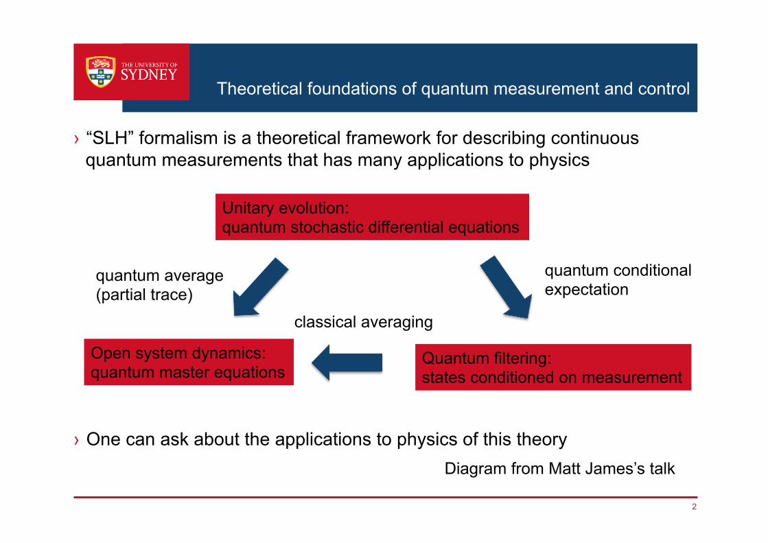
›  “SLH” formalism is a theoretical framework for describing continuous quantum measurements that has many applications to physics

› One can ask about the applications to physics of this theory

Unitary evolution: quantum stochastic differential equations

Quantum filtering: states conditioned on measurement

Open system dynamics: quantum master equations

Diagram from Matt James’s talk

quantum average (partial trace)

quantum conditional expectation

classical averaging

3

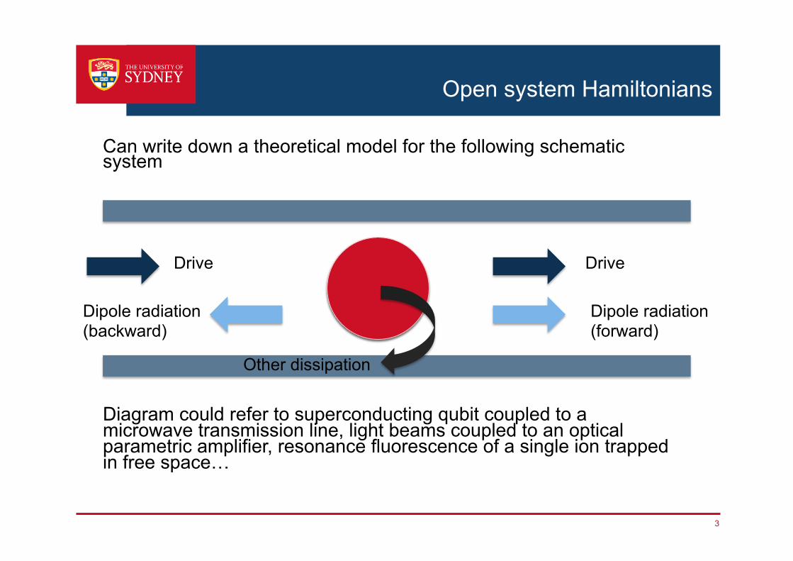
Can write down a theoretical model for the following schematic system Diagram could refer to superconducting qubit coupled to a microwave transmission line, light beams coupled to an optical parametric amplifier, resonance fluorescence of a single ion trapped in free space…

Open system Hamiltonians

Drive Drive

Dipole radiation (forward)

Dipole radiation (backward)

Other dissipation

4

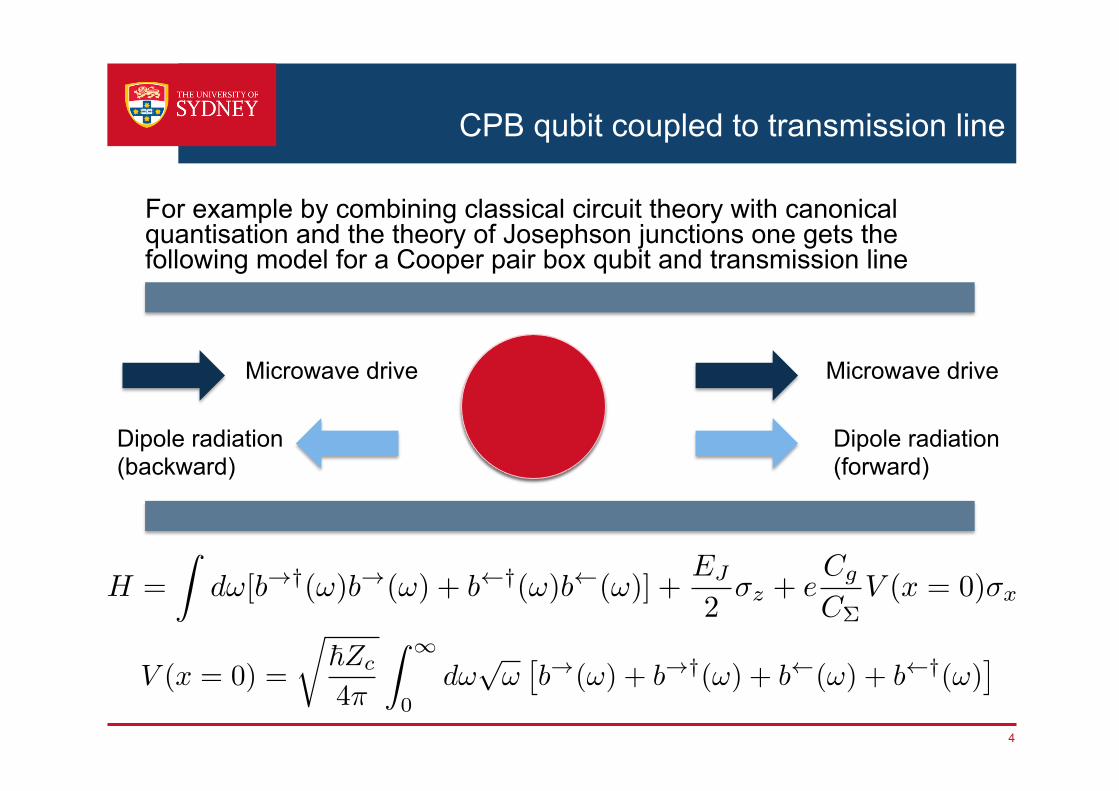
For example by combining classical circuit theory with canonical quantisation and the theory of Josephson junctions one gets the following model for a Cooper pair box qubit and transmission line

CPB qubit coupled to transmission line

Microwave drive Microwave drive

Dipole radiation (forward)

Dipole radiation (backward)

H =

Zd![b!†(!)b!(!) + b †(!)b (!)] +

EJ

2�z

+ eC

g

C⌃V (x = 0)�

x

V (x = 0) =

r~Zc

4⇡

Z 1

0d!

p!

⇥b

!(!) + b

!†(!) + b

(!) + b

†(!)⇤

5

Input fields

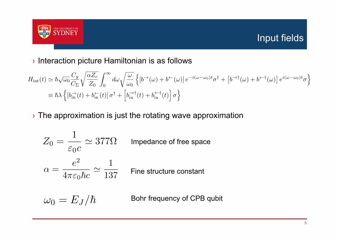
›  Interaction picture Hamiltonian is as follows

›  The approximation is just the rotating wave approximation

Hint(t) ' ~p!0Cg

C⌃

r

↵Zc

Z0

Z 1

0d!

r

!

!0

n

[b!(!) + b (!)] e�i(!�!0)t�† +⇥

b!†(!) + b †(!)⇤

ei(!�!0)t�o

⌘ ~�n

[b!in (t) + b in (t)]�† +

h

b!†in (t) + b †

in (t)i

�o

!0 = EJ/~

Impedance of free space

Fine structure constant

Bohr frequency of CPB qubit

Z0 =1

"0c' 377⌦

↵ =e2

4⇡"0~c' 1

137

6

Input fields

›  Interaction picture Hamiltonian is as follows

›  The approximation is just the rotating wave approximation

›  Picture of modes of the electromagnetic field interacting sequentially

› Or mathematically commutativity of input fields at different times

Hint(t) ' ~p!0Cg

C⌃

r

↵Zc

Z0

Z 1

0d!

r

!

!0

n

[b!(!) + b (!)] e�i(!�!0)t�† +⇥

b!†(!) + b †(!)⇤

ei(!�!0)t�o

⌘ ~�n

[b!in (t) + b in (t)]�† +

h

b!†in (t) + b †

in (t)i

�o

[bin(t), b†in(t

0)] =

Z 1

0d!d!0

p!!0

2⇡!0e�i(!�!0)tei(!

0�!0)t0[b(!), b†(!0)]

=

Z 1

�!0

d!!0 + !

2⇡!0e�i!(t�t0) ! �(t� t0)

7

Input-Output Theory

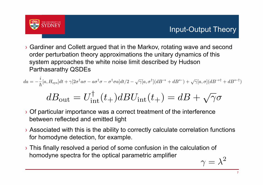
› Gardiner and Collett argued that in the Markov, rotating wave and second order perturbation theory approximations the unitary dynamics of this system approaches the white noise limit described by Hudson Parthasarathy QSDEs

› Of particular importance was a correct treatment of the interference between reflected and emitted light

›  Associated with this is the ability to correctly calculate correlation functions for homodyne detection, for example.

›  This finally resolved a period of some confusion in the calculation of homodyne spectra for the optical parametric amplifier

da = � i

~ [a,Hsys]dt+ �[2�†a� � a�†� � �†�a]dt/2�p�[a,�†](dB! + dB ) +

p�[a,�](dB!† + dB †)

dBout

= U†int

(t+

)dBUint

(t+

) = dB +p��

� = �2

8

Input-Output Theory

› Gardiner and Collett argued that in the Markov, rotating wave and second order perturbation theory approximations the unitary dynamics of this system approaches the white noise limit described by Hudson Parthasarathy QSDEs

› Of particular importance was a correct treatment of the interference between reflected and emitted light

›  Associated with this is the ability to correctly calculate correlation functions for homodyne detection, for example.

›  This finally resolved a period of some confusion in the calculation of homodyne spectra for the optical parametric amplifier

d� = � i

~ [�, Hsys]dt� ��dt/2 +p��z(dB

! + dB )

dBout

= U†int

(t+

)dBUint

(t+

) = dB +p��

� = �2

9

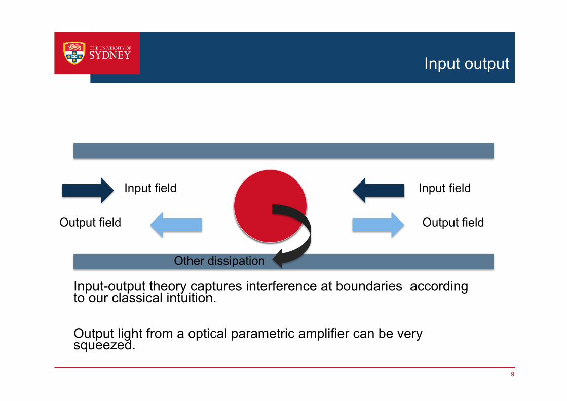
Input-output theory captures interference at boundaries according to our classical intuition. Output light from a optical parametric amplifier can be very squeezed.

Input output

Input field Input field

Output field Output field

Other dissipation

10

Input-Output theory: Rigorous statement

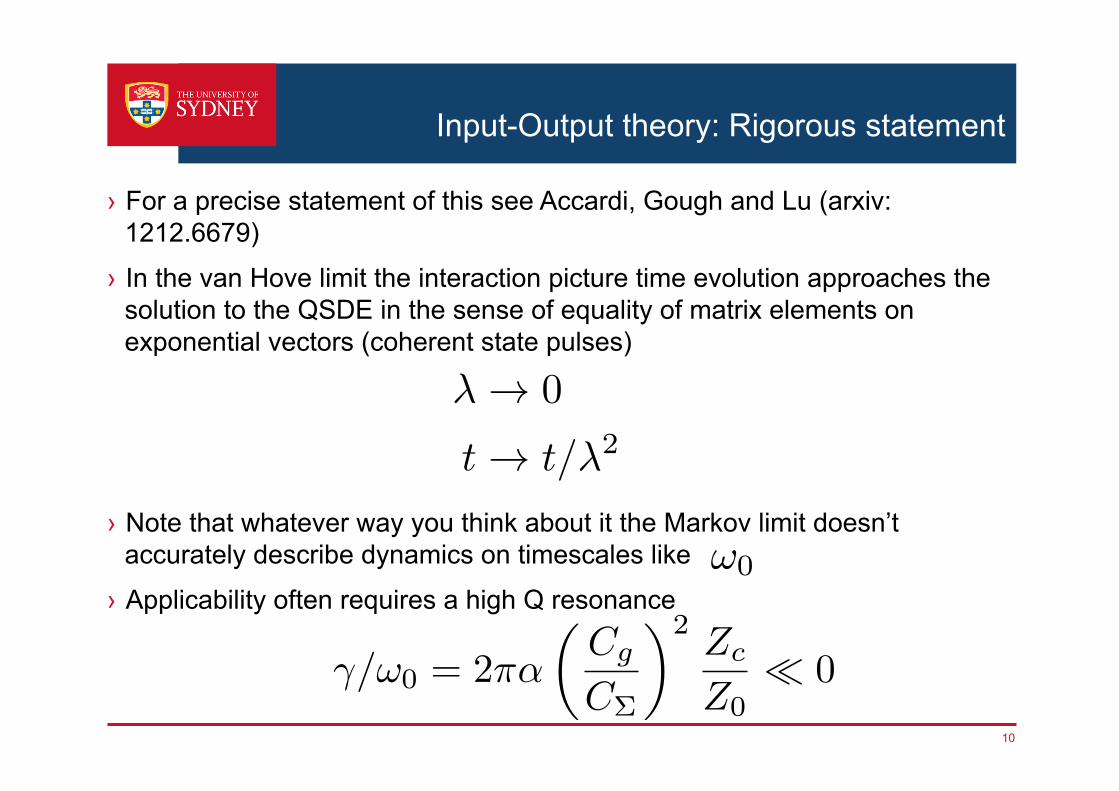
›  For a precise statement of this see Accardi, Gough and Lu (arxiv:1212.6679)

›  In the van Hove limit the interaction picture time evolution approaches the solution to the QSDE in the sense of equality of matrix elements on exponential vectors (coherent state pulses)

› Note that whatever way you think about it the Markov limit doesn’t accurately describe dynamics on timescales like

›  Applicability often requires a high Q resonance

� ! 0

t ! t/�2

!0

�/!0 = 2⇡↵

✓Cg

C⌃

◆2 Zc

Z0⌧ 0

11

“Quantum mechanics is a statistical theory”

This article reviews the various quantum-jump ap-proaches developed over the past few years. We focuson the theoretical description of basic dynamics and onsimple instructive examples rather than the applicationto numerical simulation methods.

Some of the topics covered here can also be found inearlier summaries (Erber et al., 1989; Cook, 1990;Mo” lmer and Castin, 1996; Srinivas, 1996) and more re-cent summer school lectures (Mo” lmer, 1994; Zoller andGardiner, 1995; Knight and Garraway, 1996).

II. INTERMITTENT FLUORESCENCE

Quantum mechanics is a statistical theory that makesprobabilistic predictions of the behavior of ensembles(ideally an infinite number of identically prepared quan-tum systems) using density operators. This descriptionwas completely sufficient for the first 60 years of theexistence of quantum mechanics because it was gener-ally regarded as completely impossible to observe andmanipulate single-quantum systems. For example,Schrodinger (1952) wrote. . . we never experiment with just one electron or atom or(small) molecule. In thought experiments we sometimesassume that we do; this invariably entails ridiculous con-sequences. . . . . In the first place it is fair to state that weare not experimenting with single particles, any more thanwe can raise Ichthyosauria in the zoo.

This (rather extreme) opinion was challenged by a re-markable idea of Dehmelt, which he first made public in1975 (Dehmelt, 1975, 1982). He considered the problemof high-precision spectroscopy, where one wants to mea-sure the transition frequency of an optical transition asaccurately as possible, e.g., by observing the resonancefluorescence from that transition as part (say) of anoptical-frequency standard. However, the accuracy ofsuch a measurement is fundamentally limited by thespectral width of the observed transition. The spectralwidth is due to spontaneous emission from the upperlevel of the transition, which leads to a finite lifetime t ofthe upper level. Basic Fourier considerations then implya spectral width of the scattered photons of the order oft

21. To obtain a precise value of the transition fre-quency, it would therefore be advantageous to excite ametastable transition that scatters only a few photonswithin the measurement time. On the other hand, onethen has the problem of detecting these few photons,and this turns out to be practically impossible by directobservation. Dehmelt’s proposal, however, suggests asolution to these problems, provided one would be ableto observe and manipulate single ions or atoms, whichbecame possible with the invention of single-ion traps(Paul et al., 1958; Paul, 1990) (for a review, see Horvathet al., 1997). We illustrate Dehmelt’s idea in its originalsimplified rate-equation picture. It runs as follows.

Instead of observing the photons emitted on the meta-stable two-level system directly, he proposed using anoptical double-resonance scheme as depicted in Fig. 1.One laser drives the metastable 0$2 transition while asecond strong laser saturates the strong 0$1; the life-

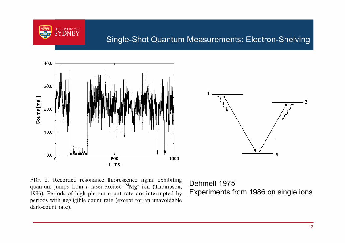
time of the upper level 1 is, for example, 1028 s, whilethat of level 2 is of the order of 1 s. If the initial state ofthe system is the lower state 0, then the strong laser willstart to excite the system to the rapidly decaying level 1,which will then lead to the emission of a photon after atime that is usually very short (of the order of the life-time of level 1). This emission restores the system to thelower level 0; the strong laser can start to excite thesystem again to level 1, which will emit a photon on thestrong transition again. This procedure repeats until atsome random time the laser on the weak transition man-ages to excite the system into its metastable state 2,where it remains shelved for a long time, until it jumpsback to the ground state, either by spontaneous emissionor by stimulated emission due to the laser on the 0$2transition. During the time the electron rests in themetastable state 2, no photons will be scattered on thestrong transition, and only when the electron jumps backto state 0 can the fluorescence on the strong transitionstart again. Therefore, from the switching on and off ofthe resonance fluorescence on the strong transition(which is easily observable), we can infer the extremelyrare transitions on the 0$2 transition. Therefore wehave a method to monitor rare quantum jumps (transi-tions) on the metastable 0$2 transition by observationof the fluorescence from the strong 0$1 transition.

A typical experimental fluorescence signal is depictedin Fig. 2 (Thompson, 1996), where the fluorescence in-tensity I(t) is plotted. However, this scheme only worksif we observe a single quantum system, because if weobserve a large number of systems simultaneously, therandom nature of the transitions between levels 0 and 2implies that some systems will be able to scatter photonson the strong transition, while others will not becausethey are in their metastable state at that moment. Froma large collection of ions observed simultaneously, onewould then obtain a more or less constant intensity ofphotons emitted on the strong transition.

The calculation of this mean intensity is a straightfor-ward task using standard Bloch equations. The calcula-

FIG. 1. The V system. Two upper levels 1 and 2 couple to acommon ground state 0. The transition frequencies are as-sumed to be largely different so that each of the two lasersdriving the system couples to only one of the transitions. The1$0 transition is assumed to be strong while the 2$0 transi-tion is weak.

102 M. B. Plenio and P. L. Knight: Quantum-jump approach to dissipative dynamics . . .

Rev. Mod. Phys., Vol. 70, No. 1, January 1998

Schroedinger, 1952

12

Single-Shot Quantum Measurements: Electron-Shelving

tion of single-system properties, such as the distributionof the lengths of the periods of strong fluorescence, re-quired some effort, which eventually led to the develop-ment of the quantum-jump approach. Apart from theinteresting theoretical implications for the study of indi-vidual quantum systems, Dehmelt’s proposal obviouslyhas important practical applications. An often-cited ex-ample is the realization of a new time standard using asingle atom in a trap. The key idea here is to use eitherthe instantaneous intensity or the photon statistics of theemitted radiation on the strong transition (the statisticsof the bright and dark periods) to stabilize the frequencyof the laser on the weak transition. This is possible be-cause the photon statistics of the strong radiation de-pends on the detuning of the laser on the weak transi-tion (Kim, 1987; Kim and Knight, 1987; Kim et al., 1987;Ligare, 1988; Wilser, 1991). Therefore a change in thestatistics of bright and dark periods indicates that thefrequency of the weak laser has shifted and has to beadjusted. However, for continuously radiating lasers thisfrequency shift will also depend on the intensity of thelaser on the strong transition. Therefore, in practice,pulsed schemes are preferable for frequency standards(Arecchi et al., 1986; Bergquist et al., 1994).

Due to the inability of experimentalists to store, ma-nipulate, and observe single-quantum systems (ions) atthe time of Dehmelt’s proposal, both the practical andthe theoretical implications of his proposal were not im-mediately investigated. It was about ten years later thatthis situation changed. At that time Cook and Kimble(1985) made the first attempt to analyze the situationdescribed above theoretically. Their advance was stimu-lated by the fact that by that time it had become possibleto actually store single ions in an ion trap (Paul trap;Paul et al., 1958; Neuhauser et al., 1980; Paul, 1990).

In their simplified rate-equation approach Cook andKimble started with the rate equations for an incoher-ently driven three-level system as shown in Fig. 1 and

assumed that the strong 0$1 transition is driven tosaturation. They consequently simplify their rate equa-tions, introducing the probabilities P1 of being in themetastable state and P2 of being in the strongly fluo-rescing 0$1 transition. This simplification now allowsthe description of the resonance fluorescence to be re-duced to that of a two-state random telegraph process.Either the atomic population is in the levels 0 and 1, andtherefore the ion is strongly radiating (on), or the popu-lation rests in the metastable level 2, and no fluores-cence is observed (off). They then proceed to calculatethe distributions for the lengths of bright and dark peri-ods and find that their distribution is Poissonian. Theiranalysis, which we have outlined very briefly here, is ofcourse very much simplified in many respects. The mostimportant point is certainly the fact that Cook andKimble assume incoherent driving and therefore adopt arate-equation model. In a real experiment coherent ra-diation from lasers is used. The complications arising incoherent excitation finally led to the development of thequantum-jump approach. Despite these problems, theanalysis of Cook and Kimble showed the possibility ofdirect observation of quantum jumps in the fluorescenceof single ions, a prediction that was confirmed shortlyafterwards in a number of experiments (Bergquist et al.,1986; Nagourney et al., 1986a, 1986b; Sauter et al., 1986a,1986b; Dehmelt, 1987) and triggered a large number ofmore detailed investigations, starting with early worksby Javanainen (1986a, 1986b, 1986c). The subsequent ef-fort of a great number of physicists eventually culmi-nated in the development of the quantum-jump ap-proach. Before we present this development in greaterdetail, we should like to study in slightly more detailhow the dynamics of the system determines the statisticsof bright and dark periods. Again assume a three-levelsystem as shown in Fig. 1. Provided the 0$1 and 0$2Rabi frequencies are small compared with the decayrates, one finds for the population in the strongly fluo-rescing level 1 as a function of time something like thebehavior shown in Fig. 3 (we derive this in detail in alater section). We choose for this figure the valuesg1@g2 for the Einstein coefficients of levels 1 and 2,which reflects the metastability of level 2. For timesshort compared with the metastable lifetime g2

21 , theatomic dynamics can hardly be aware of level 2 andevolve as a 0–1 two-level system with the ‘‘steady-state’’population r 11 of the upper level. After a time g2

21 , themetastable state has an effect, and the (ensemble-averaged) population in level 1 reduces to the appropri-ate three-level equilibrium values. The ‘‘hump’’ Dr11shown in Fig. 3 is actually a signature of the telegraphicfluorescence discussed above. To show this, consider afew sequences of bright and dark periods in the tele-graph signal as shown in Fig. 4. The total rate of emis-sion R is proportional to the rate in a bright periodtimes the fraction of the evolution made up of brightperiods. This gives

R5g1 r 11S TL

TL1TDD , (1)

FIG. 2. Recorded resonance fluorescence signal exhibitingquantum jumps from a laser-excited 24Mg+ ion (Thompson,1996). Periods of high photon count rate are interrupted byperiods with negligible count rate (except for an unavoidabledark-count rate).

103M. B. Plenio and P. L. Knight: Quantum-jump approach to dissipative dynamics . . .

Rev. Mod. Phys., Vol. 70, No. 1, January 1998

This article reviews the various quantum-jump ap-proaches developed over the past few years. We focuson the theoretical description of basic dynamics and onsimple instructive examples rather than the applicationto numerical simulation methods.

Some of the topics covered here can also be found inearlier summaries (Erber et al., 1989; Cook, 1990;Mo” lmer and Castin, 1996; Srinivas, 1996) and more re-cent summer school lectures (Mo” lmer, 1994; Zoller andGardiner, 1995; Knight and Garraway, 1996).

II. INTERMITTENT FLUORESCENCE

Quantum mechanics is a statistical theory that makesprobabilistic predictions of the behavior of ensembles(ideally an infinite number of identically prepared quan-tum systems) using density operators. This descriptionwas completely sufficient for the first 60 years of theexistence of quantum mechanics because it was gener-ally regarded as completely impossible to observe andmanipulate single-quantum systems. For example,Schrodinger (1952) wrote. . . we never experiment with just one electron or atom or(small) molecule. In thought experiments we sometimesassume that we do; this invariably entails ridiculous con-sequences. . . . . In the first place it is fair to state that weare not experimenting with single particles, any more thanwe can raise Ichthyosauria in the zoo.

This (rather extreme) opinion was challenged by a re-markable idea of Dehmelt, which he first made public in1975 (Dehmelt, 1975, 1982). He considered the problemof high-precision spectroscopy, where one wants to mea-sure the transition frequency of an optical transition asaccurately as possible, e.g., by observing the resonancefluorescence from that transition as part (say) of anoptical-frequency standard. However, the accuracy ofsuch a measurement is fundamentally limited by thespectral width of the observed transition. The spectralwidth is due to spontaneous emission from the upperlevel of the transition, which leads to a finite lifetime t ofthe upper level. Basic Fourier considerations then implya spectral width of the scattered photons of the order oft

21. To obtain a precise value of the transition fre-quency, it would therefore be advantageous to excite ametastable transition that scatters only a few photonswithin the measurement time. On the other hand, onethen has the problem of detecting these few photons,and this turns out to be practically impossible by directobservation. Dehmelt’s proposal, however, suggests asolution to these problems, provided one would be ableto observe and manipulate single ions or atoms, whichbecame possible with the invention of single-ion traps(Paul et al., 1958; Paul, 1990) (for a review, see Horvathet al., 1997). We illustrate Dehmelt’s idea in its originalsimplified rate-equation picture. It runs as follows.

Instead of observing the photons emitted on the meta-stable two-level system directly, he proposed using anoptical double-resonance scheme as depicted in Fig. 1.One laser drives the metastable 0$2 transition while asecond strong laser saturates the strong 0$1; the life-

time of the upper level 1 is, for example, 1028 s, whilethat of level 2 is of the order of 1 s. If the initial state ofthe system is the lower state 0, then the strong laser willstart to excite the system to the rapidly decaying level 1,which will then lead to the emission of a photon after atime that is usually very short (of the order of the life-time of level 1). This emission restores the system to thelower level 0; the strong laser can start to excite thesystem again to level 1, which will emit a photon on thestrong transition again. This procedure repeats until atsome random time the laser on the weak transition man-ages to excite the system into its metastable state 2,where it remains shelved for a long time, until it jumpsback to the ground state, either by spontaneous emissionor by stimulated emission due to the laser on the 0$2transition. During the time the electron rests in themetastable state 2, no photons will be scattered on thestrong transition, and only when the electron jumps backto state 0 can the fluorescence on the strong transitionstart again. Therefore, from the switching on and off ofthe resonance fluorescence on the strong transition(which is easily observable), we can infer the extremelyrare transitions on the 0$2 transition. Therefore wehave a method to monitor rare quantum jumps (transi-tions) on the metastable 0$2 transition by observationof the fluorescence from the strong 0$1 transition.

A typical experimental fluorescence signal is depictedin Fig. 2 (Thompson, 1996), where the fluorescence in-tensity I(t) is plotted. However, this scheme only worksif we observe a single quantum system, because if weobserve a large number of systems simultaneously, therandom nature of the transitions between levels 0 and 2implies that some systems will be able to scatter photonson the strong transition, while others will not becausethey are in their metastable state at that moment. Froma large collection of ions observed simultaneously, onewould then obtain a more or less constant intensity ofphotons emitted on the strong transition.

The calculation of this mean intensity is a straightfor-ward task using standard Bloch equations. The calcula-

FIG. 1. The V system. Two upper levels 1 and 2 couple to acommon ground state 0. The transition frequencies are as-sumed to be largely different so that each of the two lasersdriving the system couples to only one of the transitions. The1$0 transition is assumed to be strong while the 2$0 transi-tion is weak.

102 M. B. Plenio and P. L. Knight: Quantum-jump approach to dissipative dynamics . . .

Rev. Mod. Phys., Vol. 70, No. 1, January 1998

Dehmelt 1975 Experiments from 1986 on single ions

13

Theoretical efforts

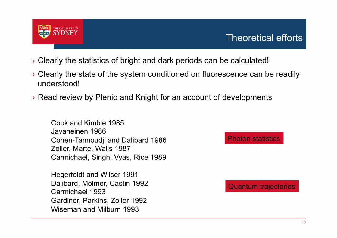
› Clearly the statistics of bright and dark periods can be calculated!

› Clearly the state of the system conditioned on fluorescence can be readily understood!

› Read review by Plenio and Knight for an account of developments

Cook and Kimble 1985 Javaneinen 1986 Cohen-Tannoudji and Dalibard 1986 Zoller, Marte, Walls 1987 Carmichael, Singh, Vyas, Rice 1989 Hegerfeldt and Wilser 1991 Dalibard, Molmer, Castin 1992 Carmichael 1993 Gardiner, Parkins, Zoller 1992 Wiseman and Milburn 1993

Photon statistics

Quantum trajectories

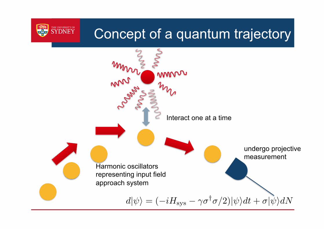
Concept of a quantum trajectory

Harmonic oscillators representing input field approach system

Interact one at a time

undergo projective measurement

d| i = (�iHsys � ��†�/2)| idt+ �| idN

15

Applications

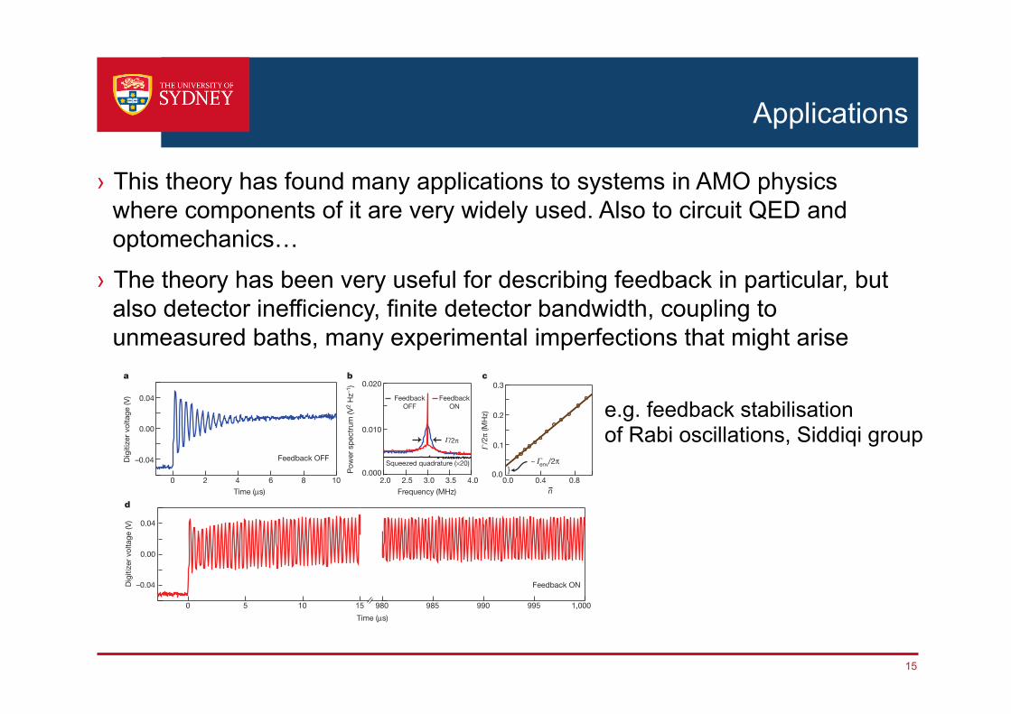
›  This theory has found many applications to systems in AMO physics where components of it are very widely used. Also to circuit QED and optomechanics…

›  The theory has been very useful for describing feedback in particular, but also detector inefficiency, finite detector bandwidth, coupling to unmeasured baths, many experimental imperfections that might arise

amplifier10,11 (paramp), which boosts the relevant quadrature to a levelcompatible with classical circuitry. The paramp output is further amp-lified and homodyne-detected (Fig. 1c) such that the amplified quad-rature (Q) contains the final measurement signal.

We obtain Rabi oscillations with the cavity continuously excited atvr/2p5 7.2749 GHz (vr < vc 2 x) with a mean cavity photon occu-pation (!n) that controls the measurement strength (see SupplementaryInformation, section II, for calibration of !n). The Rabi drive at the a.c.Stark-shifted25 qubit frequency (v01{2x!n) is turned on for a fixedduration, tm. The amplitude is adjusted to yield a Rabi frequency ofVR/2p5 3 MHz. First we average 104 measurement traces to obtain aconventional ensemble-averaged Rabi oscillation trace (Fig. 2a). Eventhough the qubit is continuously oscillating between its ground andexcited states, the oscillation phase diffuses, primarily owing to measure-ment back-action. As a result, the averaged oscillation amplitude decaysover time, but the frequency domain response retains a signature of theseoscillations26. We Fourier-transform the individual measurement tracesand plot the averaged spectrum (Fig. 2b, blue trace). A peak, centred at3 MHz and with a full-width at half-maximum of C/2p, is observed andremains unchanged even when tm is much longer than the decay time ofthe ensemble-averaged oscillations. A plot of C/2p for different mea-surement strengths (in units of !n) is shown in Fig. 2c. As expected in thedispersive regime, C and !n are linearly related25. The vertical offset isdominated by pure environmental dephasing, Cenv/2p, but has contri-butions from qubit relaxation (T1) and thermal excitation into higherqubit levels; more details can be found in Supplementary Information,sections II and IV(C).

The ratio of the height of the Rabi spectral peak to the height of thenoise floor has a theoretical maximum value of four27, correspondingto an ideal measurement with overall efficiency g 5 1. For our set-up,this efficiency can be separated into two contributions as g 5 gdetgenv.The detector efficiency is given by gdet 5 (112nadd)21, with nadd beingthe number of noise photons added by the amplification chain. The

added noise is referenced to the output of the cavity and includes theeffect of signal attenuation between the cavity and the paramp. The effectof environmental dephasing, Cenv, is modelled using genv 5 (11Cenv/CQ)21. The best measurement efficiency we obtain experimentally isg 5 0.40, with gdet 5 0.46 and genv 5 0.87; more details can be foundin Supplementary Information, section III.

We now discuss the quantum feedback protocol, which is motivatedby the classical phase-locked loop used for stabilizing an oscillator. Theamplified quadrature is multiplied by a Rabi reference signal with fre-quency V0/2p5 3 MHz using an analogue multiplier (Fig. 1d). Theoutput of this multiplier is low-pass-filtered and yields a signal propor-tional to the sine of the phase difference, herr, between the 3-MHzreference and the 3-MHz component of the amplified quadrature.This ‘phase error’ signal is fed back to control the Rabi frequency VR

by modulating the Rabi drive strength with an upconverting IQ mixer(Fig. 1a). The amplitude of the reference signal controls the dimension-less feedback gain, F, through the expression Vfb/VR 5 2Fsin(herr),where Vfb is the change in Rabi frequency due to feedback. Figure 2dshows the ensemble-averaged, feedback-stabilized oscillation, whichpersists for much longer than the original oscillation in Fig. 2a. In fact,within the limits imposed by our maximum data acquisition time of20 ms, these oscillations persist indefinitely. The red trace in Fig. 2bshows the corresponding averaged spectra. The needle-like peak at3 MHz is the signature of the stabilized Rabi oscillations.

To confirm the quantum nature of the feedback-stabilized oscillations,we perform state tomography on the qubit28. We stabilize the dynamicalqubit state, stop the feedback and Rabi driving after a fixed time (80ms 1ttomo after starting the Rabi drive), and then measure the projection ofthe quantum state along one of three orthogonal axes. This is done usingstrong measurements (by increasing !n) with high single-shot fidelity11.This allows us to remove any data points where the qubit was found inthe second excited state (Supplementary Information, section IV(C)).By repeating this many times, we can determine ÆsXæ, ÆsYæ and ÆsZæ,

Feedback ONDig

itize

r vol

tage

(V)

Time (μs)

–0.04

0.00

0.04

151050 1,000995990985980

–0.04

0.00

0.04

1086420

Dig

itize

r vol

tage

(V)

Time (μs)

Feedback OFF

a

d

b0.020

0.010

0.0004.03.53.02.52.0

Pow

er s

pect

rum

(V2

Hz–1

)

Frequency (MHz)

/2π

FeedbackOFF

FeedbackON

Squeezed quadrature (×20)

/2π

(MH

z)n

c0.3

0.2

0.1

0.00.80.40.0

~ env/2π}

Γ

Γ

Γ

Figure 2 | Rabi oscillations and feedback. a, We average 104 measurementtraces using weak continuous measurement and simultaneous Rabi driving toobtain ensemble-averaged Rabi oscillations that decay in time as a result ofensemble dephasing. b, Averaged Fourier transforms of the individualmeasurement traces from a. The spectrum shows a peak at the Rabi frequency(blue trace) with a full-width at half-maximum of C/2p. The grey trace showsan identically prepared spectrum for the squeezed quadrature (multiplied by 20for clarity), which contains no qubit state information. c, C/2p plotted as afunction of cavity photon occupation, !n (measurement strength), showing the

expected linear dependence. The vertical offset is dominated by pureenvironmental dephasing, Cenv/2p, but has contributions from qubit relaxation(T1) and thermal excitation into higher qubit levels. d, Feedback-stabilized,ensemble-averaged Rabi oscillations, which persist for much longer times thanthose without feedback (a). The corresponding spectrum, shown in b, has aneedle-like peak at the Rabi reference frequency (red trace). The slowlychanging mean level in the Rabi oscillation traces in a and d is due to thethermal transfer of population into the second excited state of the qubit. SeeSupplementary Information, section IV(C), for more details.

RESEARCH LETTER

7 8 | N A T U R E | V O L 4 9 0 | 4 O C T O B E R 2 0 1 2

Macmillan Publishers Limited. All rights reserved©2012

e.g. feedback stabilisation of Rabi oscillations, Siddiqi group

16

Beyond second order

› Many physicists are allergic to the set of approximations that are used to reach this theory

›  There are many alternative methods for dealing with open quantum systems that do not necessarily make these approximations, but usually no analog of the conditioned state is available (eg Leggett et al Rev Mod Phys)

› My prejudice is that this theory is too useful to ignore and more widely applicable than is usually appreciated

› However important insights as to how to proceed may be gained from some of these alternative approaches

›  For example the model we have discussed corresponds to the “anisotropic Kondo model” and has been very widely studied.

17

Some higher order approaches

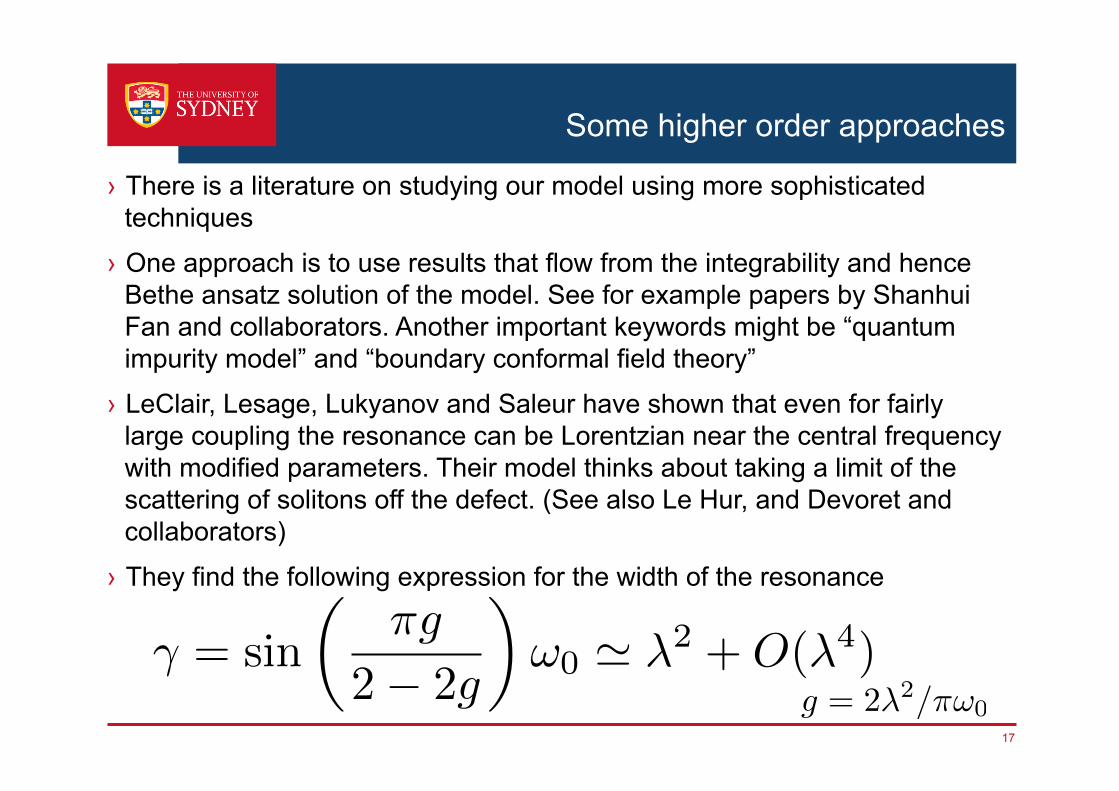
›  There is a literature on studying our model using more sophisticated techniques

› One approach is to use results that flow from the integrability and hence Bethe ansatz solution of the model. See for example papers by Shanhui Fan and collaborators. Another important keywords might be “quantum impurity model” and “boundary conformal field theory”

›  LeClair, Lesage, Lukyanov and Saleur have shown that even for fairly large coupling the resonance can be Lorentzian near the central frequency with modified parameters. Their model thinks about taking a limit of the scattering of solitons off the defect. (See also Le Hur, and Devoret and collaborators)

›  They find the following expression for the width of the resonance

� = sin

✓⇡g

2� 2g

◆!0 ' �2 +O(�4)

g = 2�2/⇡!0

18

Toward Controllable Markov Approximation

›  The detector should be located well away from the system and there will be an approximation where these modes approximately commute close to some central frequency, as before, and can be described in a white noise limit.

›  The times of these output fields will only label arrival at the detector, interaction at the system will be at some indefinite time, cf current situation

›  Is it possible to write a conditioned state for the system under these circumstances?