Quantum Spin and Local Reality - viXravixra.org/pdf/1408.0005v2.pdfAlmost a century ago Stern-Gerlach laid important foundations for quantum mechanics. Based on these, Bell formulated

.193

Quantum Spin and Local Reality

A Quantum Theory of Events

© Edwin Eugene Klingman

8/5/2014

Almost a century ago Stern-Gerlach laid important foundations for quantum mechanics. Based on these, Bell formulated a model of local hidden variables, which is supposed to describe "all possible ways" in which classical systems can generate results, but Bell did not consider one possibility in which classical behavior leads to quantum results. Bell buried the key fact needed to challenge his logic: the θ -dependence of two energy modes: rotation and deflection. An Energy-Exchange theorem is presented and proved: if 0≠dtdθ the implied time-evolution will affect expectation values and the essentially classical mechanism yields quantum correlations ba ⋅− . Analysis of the spin-component measurement brings Bell’s counterfactual logic into question. I show that Watson’s formal linking of time-evolution operator to measurement operation addresses Bell's stated concerns about measurement in quantum mechanics and produces the ba ⋅− correlation. Our results, restricted to particle spin, have wider implications, including relevance to the ontic versus epistemic issues currently debated in the literature. The suggested formalism extends beyond Stern-Gerlach to other quantum mechanical processes characterized by a 'jump' or 'collapse of the wave function'.

Table of Contents Abstract ......................................................................................................................................................... 5

An Overview—50 years of Bell’s Theorem .................................................................................................... 6

Bell’s Theorem .......................................................................................................................................... 6

Spin: Classical and Quantum ..................................................................................................................... 7

The Experiment ........................................................................................................................................... 10

The Quantum Analysis ............................................................................................................................ 12

Exactly what is precessing? ..................................................................................................................... 16

The Classical Model ................................................................................................................................. 17

Positivism or Realism? ................................................................................................................................ 20

Basic Physical Assumptions about Degrees of Freedom ....................................................................... 21

Does deflection in a magnetic field require energy? .............................................................................. 24

Classical Analysis of Precessing in Stern-Gerlach ........................................................................................ 26

Quantum Analysis of Stern-Gerlach ........................................................................................................... 30

More complex spin interactions ............................................................................................................. 34

Is Stern-Gerlach really a 'quantum' measurement? ................................................................................... 35

Susskind's first Quantum Mechanics Lecture of Theoretical Minimum ................................................. 35

An Energy Exchange Theorem .................................................................................................................... 38

Does the Angle of Precession Change? ....................................................................................................... 39

Is Stern-Gerlach a dissipative system? .................................................................................................... 39

The extended Stern-Gerlach apparatus .................................................................................................. 41

New Field-theoretical Facts? .................................................................................................................. 45

Conservation of Energy and Momentum................................................................................................ 47

Quantum caveat.......................................................................................................................................... 49

Bell’s Theorem ............................................................................................................................................ 50

”Disproof” of Bell’s Theorem .................................................................................................................. 51

Formulation of Bell’s Theorem ............................................................................................................... 52

Our ‘hidden variable’ .............................................................................................................................. 52

The Quantum Theory of Events .................................................................................................................. 53

Energy Modes Coupled to a Common Variable .......................................................................................... 55

The Energy-Exchange Theorem .............................................................................................................. 55

The transfer of locally conserved energy ................................................................................................ 58

2

The Energy-Exchange Theorem and the change of precessional energy ............................................... 59

If it gains .............................................................................................................................................. 59

If it loses .............................................................................................................................................. 59

Where does it go? ............................................................................................................................... 60

Quantum Precession ................................................................................................................................... 61

Quantum Transformation theory ............................................................................................................... 62

Watson’s Q-operator .............................................................................................................................. 63

Watson’s refutation of Bell’s Theorem ................................................................................................... 64

Local realism in the quantum theory of events ...................................................................................... 67

The Perspective of Local Realism ................................................................................................................ 68

Dynamic Equivalence Classes .................................................................................................................. 69

Q-operator and Probability ..................................................................................................................... 70

Q-operator Probability Distributions ...................................................................................................... 71

An Event-based Interpretation of Quantum Mechanics ............................................................................ 73

The Geometry ......................................................................................................................................... 75

The Algebra ............................................................................................................................................. 77

The Formal Nature of the Wave Function .................................................................................................. 79

Constructing the quantum mechanics of spin ........................................................................................ 81

The Quantum Nature of the Wave Function .............................................................................................. 83

Is Watson’s formalism compatible with quantum mechanics? .............................................................. 87

Consequences of the Standard Formalism ............................................................................................. 88

No Epistemic Model Can Fully Explain… ................................................................................................. 89

The Physical Nature of the Wave Function ................................................................................................. 92

A Geometric Algebra Perspective ............................................................................................................... 95

Wave Function and Superposition .......................................................................................................... 98

‘Measurement’ and ‘Experiment’ ............................................................................................................. 101

The Canonical Counter and Information .............................................................................................. 104

Summary: Quantum Theory of Events ..................................................................................................... 105

The ‘jump’ operator goes beyond Bell's theorem and Stern-Gerlach .................................................. 107

The Confused Understanding of Quantum Mechanics ............................................................................. 109

The Underlying State ............................................................................................................................ 110

The Structure of Reality ........................................................................................................................ 111

3

But is it realistic? ................................................................................................................................... 112

Remember what’s at stake ....................................................................................................................... 113

Born Rule and Bayesian Probability .......................................................................................................... 114

Enter Counterfactuality ............................................................................................................................. 116

Bell’s theorem is based on counterfactual logic ....................................................................................... 118

Asher Peres ‘counterfactual’ quotes..................................................................................................... 120

The source of the counterfactual problem ........................................................................................... 121

Entanglement and Steering ...................................................................................................................... 122

Brief summary .......................................................................................................................................... 126

Conclusion: the Quantum Theory of Events ............................................................................................. 127

The cup overfloweth ................................................................................................................................. 131

Acknowledgments ..................................................................................................................................... 132

References ................................................................................................................................................ 132

4

Quantum Spin and Local Reality © Edwin Eugene Klingman

Abstract

Almost a century ago Stern-Gerlach laid important foundations for quantum mechanics. Based on these, Bell formulated a model of local hidden variables, which is supposed to describe "all possible ways" in which classical systems can generate results, but Bell did not consider one possibility in which classical behavior leads to quantum results. Bell buried the key fact needed to challenge his logic: the θ -dependence of two energy modes: rotation and deflection. An Energy-Exchange theorem is presented and proved: if 0≠dtdθ the implied time-evolution will affect expectation values and an essentially classical mechanism yields quantum correlations ba ⋅− . Analysis of the spin-component measurement brings Bell’s counterfactual logic into question. I show that Watson’s formal linking of time-evolution operator to measurement operation addresses Bell's stated concerns about measurement in quantum mechanics and produces the ba ⋅− correlation. Our results, restricted to particle spin, have wider implications, including relevance to the ontic versus epistemic issues currently debated in the literature. The suggested formalism extends beyond Stern-Gerlach to other quantum mechanical processes characterized by a 'jump' or 'collapse of the wave function'.

5

An Overview—50 years of Bell’s Theorem Two conceptual revolutions in physics are approaching major anniversaries – the 100th anniversary of Einstein's 1916 general relativity theory and the 50th anniversary of John Bell's 1964 theory1 about local realism. The significance of these revolutions is their challenge to intuitive understand-ing of reality. Classical physics is largely compatible with our intuition. The few exceptions, like action-at-a-distance, trace primarily to a static treatment of a dynamic reality. Einstein’s relativistic denial of simultaneity left the realm of intuition entirely. And Bell's denial of local realism left all physicists confused, confirming Feynman's claim that no one understands quantum mechanics. This paper reviews the concept of local realism analyzed by Bell and challenges to Bell's theorem. To do so requires a definition of local realism and the concepts of spin, both classical and quantum. Local realism refers to the intuitively obvious fact that physically real things in one location do not and cannot instantaneously affect other physically real things at a remote location. Based on his analysis of 'quantum spin', John S Bell, in 1964, claimed that local realism does not exist. He did so by analyzing a physics experiment and deriving a result that fails to agree with the actual measured results. On the basis of the model’s failure to accurately describe the way Nature behaves, he concludes there is no local reality.

Bell’s Theorem On this 50th anniversary of Bell's theorem there is no shortage of papers about Bell's theorem; each paper tending to become a little more obtuse than the last one, so we focus first on the physics of Bell's theorem, based on Stern-Gerlach. Assume that λ represents a locally real physical property of a particle, and let the physics involve a pair of such particles created in such a way that angular momentum (spin) is conserved and sums to zero. In relevant experiments Alice sets her instrument to a , denoted )(aA while Bob independently chooses b

for

his setting, )(bB

. Alice measures A , which yields 1+ or 1− , and Bob measures B . The term λ is what all the excitement is about. It represents the physics of the situation, while a and b

represent freely chosen, independent settings of

the experimental apparatus. Bell defines λ very broadly, allowing it to be continuous or discrete, scalar or vector, etc. Whatever its form, λ should explain how Alice's particle and Bob's particle are correlated in such a way that the product of measurements yields

babBaA⋅−=⟩⟨ ),(),( λλ 1- 1

6

because this is the result of a quantum mechanical formulation of the problem and it agrees with the correlated measurement data. Bell is searching for a classical explanation of this result. As there is no visible mechanism in quantum mechanics, λ is called a ‘hidden variable’ . Correlated measurements are based on the assumption that Alice and Bob freely choose their own settings and no information is exchanged between remote measure-ment stations until after the experiment has been performed. Bell asked if any classical property, common to both Alice and Bob can match the experiment-ally found measurement correlations.

This is Bell’s theorem: it is impossible to find such a λ . We will analyze Bell’s theorem, but first we review the classical and quantum physics of spin, on which the key experiment is based.

Spin: Classical and Quantum Key particle properties are mass, spin, and charge. Classically these properties are well-defined, but, although spin is visualizable as a spinning top, problems arise when the model is interpreted through quantum mechanics. Though first encountered experimentally by Stern and Gerlach, these are still unresolved. And although particle spin was initially used primarily to interpret fine-splitting of atomic spectra, today Xiao and Bauer note4 that

"Spintronics is all about manipulation and transport of the spin, the intrinsic angular momentum of the electron. These two tasks are incompatible, since manipulation requires strong coupling of the spin with the outside world, which perturbs (spin) transport over long distances."

This certainly seems to apply to the Stern-Gerlach experiment, in which the ‘outside world’ (the inhomogeneous magnets) ‘perturbs’ transport of the spin. Macroscopic spin is associated with tops and gyroscopes. A ‘top’ is a classical spinning particle, of arbitrary shape. Mathematically, this is called a trivector. Analysis of its motion forms a significant portion of classical mechanics. A gyroscope is a constrained particle with well-defined reference frames in terms of which torque and forces are analyzed. But there is a huge conceptual mis-match between classical rotor and quantum spin. We examine this mismatch in some detail, beginning with the classical definition of angular momentum as a 3D vector, prL

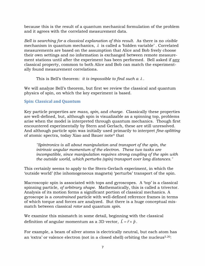
×= . For example, a beam of silver atoms is electrically neutral, but each atom has an ‘extra’ or valence electron (not in a closed shell) orbiting the nucleus5.20:

7

This creates a magnetic moment (current loop). The reader is assumed familiar with classical spin but somewhat confused by quantum mechanical spin, and associated quantum concepts of probability wave functions, Heisenberg’s un-certainty principle, Dirac half-integer spin, the lack of the classically expected continuous output from the Stern-Gerlach device, plus superposition, interfer-ence, collapse of the wave function, and other aspects of quantum mechanics. These predispose most physicists to accept one more weird feature of quantum mechanics: Bell's inequality, which effectively does away with local realism.

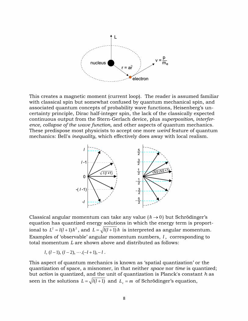
Classical angular momentum can take any value ( 0→ ) but Schrödinger’s equation has quantized energy solutions in which the energy term is proport-ional to 22 )1( += llL , and )1( += llL is interpreted as angular momentum. Examples of ‘observable’ angular momentum numbers, l , corresponding to total momentum L are shown above and distributed as follows:

lllll −+−−− ),1.(),2(),1(, .

This aspect of quantum mechanics is known as ‘spatial quantization’ or the quantization of space, a misnomer, in that neither space nor time is quantized; but action is quantized, and the unit of quantization is Planck's constant h as seen in the solutions )1( += llL and mLz = of Schrödinger’s equation,

8

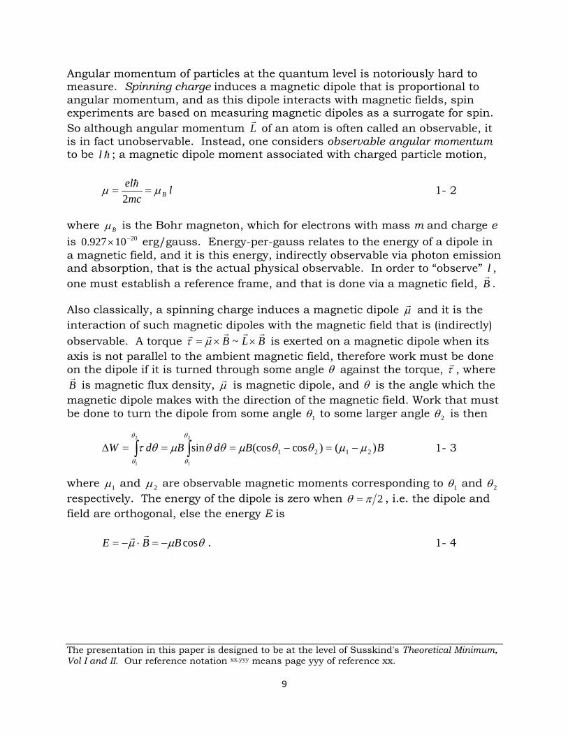
Angular momentum of particles at the quantum level is notoriously hard to measure. Spinning charge induces a magnetic dipole that is proportional to angular momentum, and as this dipole interacts with magnetic fields, spin experiments are based on measuring magnetic dipoles as a surrogate for spin. So although angular momentum L

of an atom is often called an observable, it

is in fact unobservable. Instead, one considers observable angular momentum to be l ; a magnetic dipole moment associated with charged particle motion,

lmc

elBµµ ==

2 1- 2

where Bµ is the Bohr magneton, which for electrons with mass m and charge e is 2010927.0 −× erg/gauss. Energy-per-gauss relates to the energy of a dipole in a magnetic field, and it is this energy, indirectly observable via photon emission and absorption, that is the actual physical observable. In order to “observe” l , one must establish a reference frame, and that is done via a magnetic field, B

.

Also classically, a spinning charge induces a magnetic dipole µ and it is the interaction of such magnetic dipoles with the magnetic field that is (indirectly) observable. A torque BLB

××= ~µτ is exerted on a magnetic dipole when its

axis is not parallel to the ambient magnetic field, therefore work must be done on the dipole if it is turned through some angle θ against the torque, τ , where B

is magnetic flux density, µ is magnetic dipole, and θ is the angle which the magnetic dipole makes with the direction of the magnetic field. Work that must be done to turn the dipole from some angle 1θ to some larger angle 2θ is then

BBdBdW )()cos(cossin 2121

2

1

2

1

µµθθµθθµθτθ

θ

θ

θ

−=−===∆ ∫∫ 1- 3

where 1µ and 2µ are observable magnetic moments corresponding to 1θ and 2θ respectively. The energy of the dipole is zero when 2πθ = , i.e. the dipole and field are orthogonal, else the energy E is

θµµ cosBBE −=⋅−=

. 1- 4 The presentation in this paper is designed to be at the level of Susskind's Theoretical Minimum, Vol I and II. Our reference notation xx.yyy means page yyy of reference xx.

9

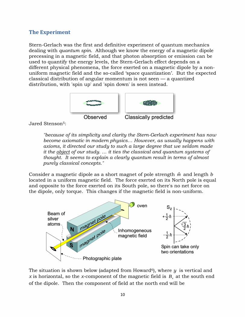
The Experiment Stern-Gerlach was the first and definitive experiment of quantum mechanics dealing with quantum spin. Although we know the energy of a magnetic dipole precessing in a magnetic field, and that photon absorption or emission can be used to quantify the energy levels, the Stern-Gerlach effect depends on a different physical phenomena, the force exerted on a magnetic dipole by a non-uniform magnetic field and the so-called ‘space quantization’. But the expected classical distribution of angular momentum is not seen — a quantized distribution, with 'spin up' and 'spin down' is seen instead.

Jared Stenson5:

"because of its simplicity and clarity the Stern-Gerlach experiment has now become axiomatic in modern physics… However, as usually happens with axioms, it directed our study to such a large degree that we seldom made it the object of our study. … it ties the classical and quantum systems of thought. It seems to explain a clearly quantum result in terms of almost purely classical concepts."

Consider a magnetic dipole as a short magnet of pole strength m and length b located in a uniform magnetic field. The force exerted on its North pole is equal and opposite to the force exerted on its South pole, so there's no net force on the dipole, only torque. This changes if the magnetic field is non-uniform.

The situation is shown below (adapted from Howard6), where y is vertical and x is horizontal, so the x-component of the magnetic field is xB at the south end of the dipole. Then the component of field at the north end will be

10

zx

yx

xx

x bz

Bb

yB

bx

BB

∂∂

+∂∂

+∂∂

+ 1- 5

where xb , yb , and zb are the projections of b

on the respective axes.

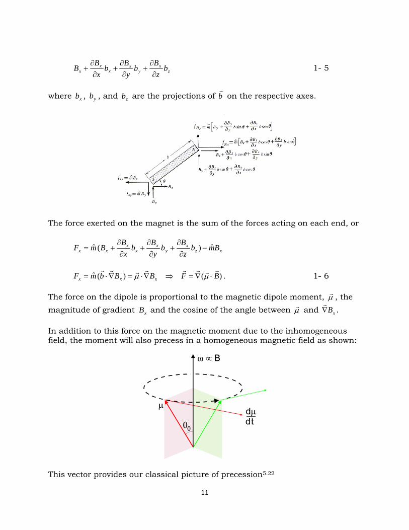
The force exerted on the magnet is the sum of the forces acting on each end, or

xzx

yx

xx

xx Bmbz

Bb

yB

bx

BBmF ˆ)(ˆ −

∂∂

+∂∂

+∂∂

+=

)()(ˆ BFBBbmF xxx

⋅∇=⇒∇⋅=∇⋅= µµ . 1- 6

The force on the dipole is proportional to the magnetic dipole moment, µ , the magnitude of gradient xB and the cosine of the angle between µ and xB∇

.

In addition to this force on the magnetic moment due to the inhomogeneous field, the moment will also precess in a homogeneous magnetic field as shown:

This vector provides our classical picture of precession5.22

11

The Quantum Analysis There are, however, major conceptual problems, as Stenson indicates5.2:

"In the textbooks forces, trajectories, precessing vectors are all used to make the description clear, while on another page we’re forbidden to speak of such things in quantum descriptions." (see 9.188)

Stanford professor Leonard Susskind has produced a well-received YouTube series and published two books in the series2,3: The Theoretical Minimum. In Vol. 2: Quantum Mechanics, he says essentially the same thing:3.3

"… spin can be pictured as a little arrow that points in some direction, but that naïve picture is too classical to accurately represent the real situation. The spin of an electron is about as quantum mechanical as a system can be, and any attempt to visualize it classically will badly miss the point."

Why is this so? In his lectures Susskind introduces it as a ‘qubit’ or quantum bit rather than as physical spin, and treats it as a two state system or “a bit". He notes that an experiment involves not only the system to be measured, but an apparatus—a two state device that records 'up' or 'down' (+1 or -1). He notes that, if spin is a vector, it should have three components xσ , yσ , and zσ , and when we measure the spin to be pointing in the z -direction, we expect to find

xσ or yσ to be zero. But if the apparatus is pointed in the x or y direction, it still produces 1± . Yet, the average of xσ measurements performed on a 1=zσ spin will yield zero, and the average of zσ measurements performed on a 1=zσ spin will yield +1. Also the average of measurements performed at an angle θ to the z-axis will yield θcos . This is not classical behavior. Moreover, as long as zσ is measured, the state remains unchanged, but any other measurement will restore the system to a state of uncertainty (although the average of successive measurements yields the value expected for a component in that direction, if repeatedly reset to z, then measured at θ ). Susskind:

"… one simply cannot simultaneously know the components of the spin along two different axes… There is something fundamentally different about the state of a quantum system and the state of classical system."

The question is: does this simply reflect the fundamentally different quantum and classical measurement apparatus? In most treatments the nature of the measurement device is vastly under-emphasized. That we're using a 1D device to measure a 3D spin is glossed over. Consider an analogy with quantum fishermen using a 2D device to measure 3D fish, and concluding that all fish

12

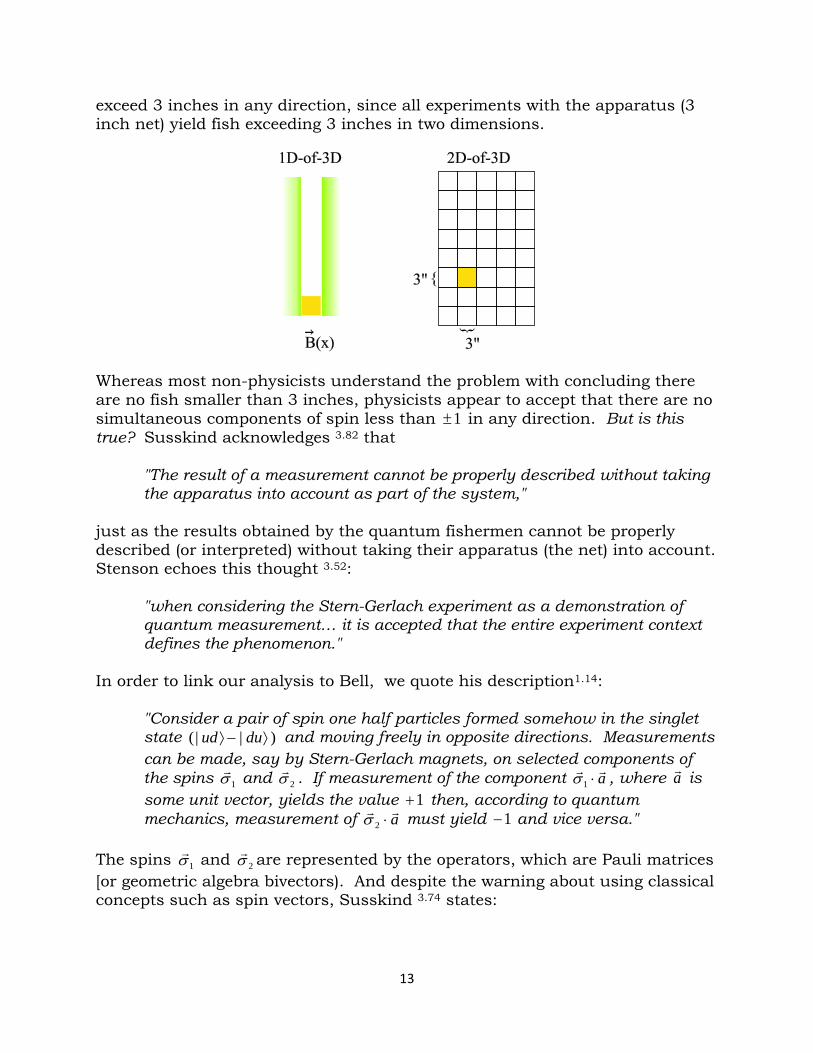
exceed 3 inches in any direction, since all experiments with the apparatus (3 inch net) yield fish exceeding 3 inches in two dimensions.

Whereas most non-physicists understand the problem with concluding there are no fish smaller than 3 inches, physicists appear to accept that there are no simultaneous components of spin less than 1± in any direction. But is this true? Susskind acknowledges 3.82 that

"The result of a measurement cannot be properly described without taking the apparatus into account as part of the system,"

just as the results obtained by the quantum fishermen cannot be properly described (or interpreted) without taking their apparatus (the net) into account. Stenson echoes this thought 3.52:

"when considering the Stern-Gerlach experiment as a demonstration of quantum measurement… it is accepted that the entire experiment context defines the phenomenon."

In order to link our analysis to Bell, we quote his description1.14:

"Consider a pair of spin one half particles formed somehow in the singlet state )||( ⟩−⟩ duud and moving freely in opposite directions. Measurements can be made, say by Stern-Gerlach magnets, on selected components of the spins 1σ

and 2σ . If measurement of the component a⋅1σ , where a is

some unit vector, yields the value 1+ then, according to quantum mechanics, measurement of a

⋅2σ must yield 1− and vice versa." The spins 1σ

and 2σ are represented by the operators, which are Pauli matrices [or geometric algebra bivectors). And despite the warning about using classical concepts such as spin vectors, Susskind 3.74 states:

13

"An operator associated with the measurement of a vector (spin) has a vector character of its own."

Stop and think about that…

"Because their components are real valued, 3-vectors are not quite rich enough to represent quantum states. (…) What sort of vector is the spin operator σ ? It is definitely not a state-vector [a bra or a ket]. It's not exactly a 3-vector either … but it's associated with the direction in space. But … just as a spin-measuring apparatus can only answer questions about a spin's orientation in a specific direction, a spin operator can only provide information about the spin component in a specific direction. To physically measure spin in a different direction, we need to rotate the apparatus to point in the new direction …there is a spin operator for each direction in which the apparatus can be oriented."

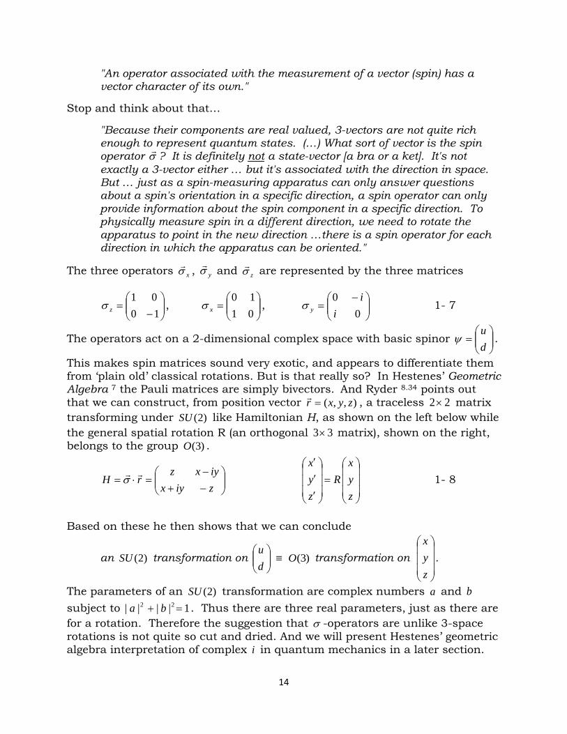
The three operators xσ , yσ and zσ are represented by the three matrices

−

=1001

zσ ,

=

0110

xσ ,

−=

00i

iyσ 1- 7

The operators act on a 2-dimensional complex space with basic spinor

=

du

ψ .

This makes spin matrices sound very exotic, and appears to differentiate them from ‘plain old’ classical rotations. But is that really so? In Hestenes’ Geometric Algebra 7 the Pauli matrices are simply bivectors. And Ryder 8.34 points out that we can construct, from position vector ),,( zyxr =

, a traceless 22× matrix transforming under )2(SU like Hamiltonian H, as shown on the left below while the general spatial rotation R (an orthogonal 33× matrix), shown on the right, belongs to the group )3(O .

−+−

=⋅=ziyxiyxz

rH σ

=

′′′

zyx

Rzyx

1- 8

Based on these he then shows that we can conclude

an )2(SU transformation on

du

≡ )3(O transformation on

zyx

.

The parameters of an )2(SU transformation are complex numbers a and b subject to 1|||| 22 =+ ba . Thus there are three real parameters, just as there are for a rotation. Therefore the suggestion that σ -operators are unlike 3-space rotations is not quite so cut and dried. And we will present Hestenes’ geometric algebra interpretation of complex i in quantum mechanics in a later section.

14

But there are other differences peculiar to quantum mechanics. For example Griffiths explains 9.27 that if the expectation value is ⟩⟨≡⟩⟨ ψψ ||ˆ AA and xA ˆˆ =

"[This] emphatically does not mean that if you measure the position of one particle over and over again, ⟩⟨ x is the average of the results… Rather, ⟩⟨ x is the average of measurements performed on all particles all in the state ψ , which means you must find some way of returning the particle to its original state after each measurement, or else you prepare a whole ensemble particles, each in the same state ψ , and measure the positions of all of them: ⟩⟨ x is the average of these results…"

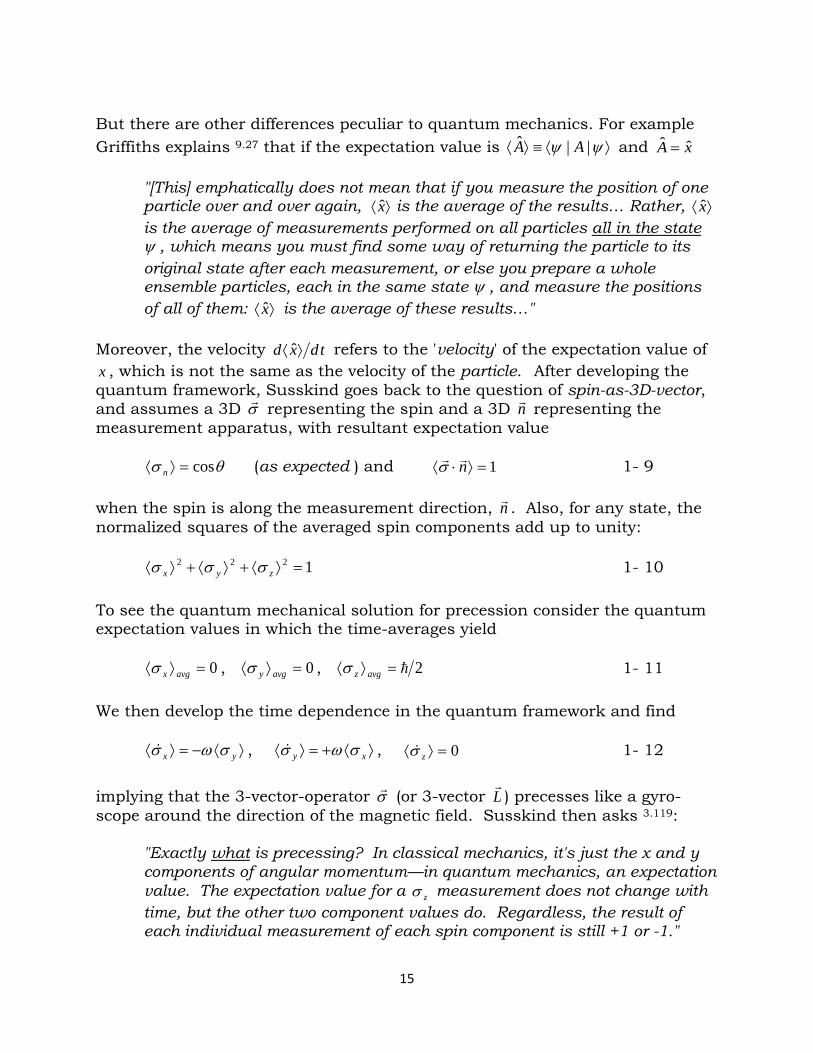
Moreover, the velocity tdxd ⟩⟨ ˆ refers to the 'velocity' of the expectation value of x , which is not the same as the velocity of the particle. After developing the quantum framework, Susskind goes back to the question of spin-as-3D-vector, and assumes a 3D σ representing the spin and a 3D n representing the measurement apparatus, with resultant expectation value

θσ cos=⟩⟨ n (as expected ) and 1=⟩⋅⟨ nσ 1- 9

when the spin is along the measurement direction, n . Also, for any state, the normalized squares of the averaged spin components add up to unity:

1222 =⟩⟨+⟩⟨+⟩⟨ zyx σσσ 1- 10 To see the quantum mechanical solution for precession consider the quantum expectation values in which the time-averages yield

0=⟩⟨ avgxσ , 0=⟩⟨ avgyσ , 2=⟩⟨ avgzσ 1- 11 We then develop the time dependence in the quantum framework and find

⟩⟨−=⟩⟨ yx σωσ , ⟩⟨+=⟩⟨ xy σωσ , 0=⟩⟨ zσ 1- 12 implying that the 3-vector-operator σ (or 3-vector L

) precesses like a gyro-

scope around the direction of the magnetic field. Susskind then asks 3.119:

"Exactly what is precessing? In classical mechanics, it's just the x and y components of angular momentum—in quantum mechanics, an expectation value. The expectation value for a zσ measurement does not change with time, but the other two component values do. Regardless, the result of each individual measurement of each spin component is still +1 or -1."

15

So in classical mechanics, real objects precess, but in quantum mechanics only statistical objects behave in the same way as real classical objects. This fact underlies Feynman's famous remark about no one understanding QM. A schizophrenia was built into quantum mechanics by Bohr and Heisenberg: quantum phenomena, at least in terms of experiments, must be described in plain language. Heisenberg10.17:

"Any experiment in physics, whether it refers to the phenomenon of daily life or atomic events, is to be described in terms of classical physics."

As Stenson explains 5.47:

"in other words, the common opinion is that although nature fundamentally behaves quantum mechanically humans can only understand it in terms of classical concepts."

Humans understand a thing at a time, while quantum mechanics treats not "things", but only statistical summaries of measurements on things. Susskind asked the key question:

Exactly what is precessing?

Either a real classical object or statistical quantum object appears to precess. In lectures, Susskind several times focuses on the precession of the spin in a magnetic field, maintaining that only absorption or emission of photons will cause the angle the spin makes with the magnetic field B

to change. But we do

not observe the emission or absorption of photons. Does this mean that spin continues to precess? That seems to be his implication, but is it true? The question ‘what is precessing?’ implies significant confusion surrounding the physics of Stern-Gerlach. The key fact that is interpreted as establishing the 'quantum' nature of spin is that the particles traversing the field are found at two discrete positions (up and down) as opposed to the continuous distrib-ution expected from a classical treatment. This is interpreted as demonstrating that the spin is quantized, existing only in spin up or spin down states. Two facts complicate this seeming agreement with Schrödinger’s space quantization. Heisenberg’s uncertainty principle implies one cannot measure one component of the spin without disturbing other components of the spin; the fact is that the measuring apparatus has only one degree of freedom, or spin direction. So, in analogous manner, scientists employing a 'quantized' filter will conclude "fish are quantized", since all experiments performed with this apparatus yield fish greater than or equal to 3 inches in any direction.

16

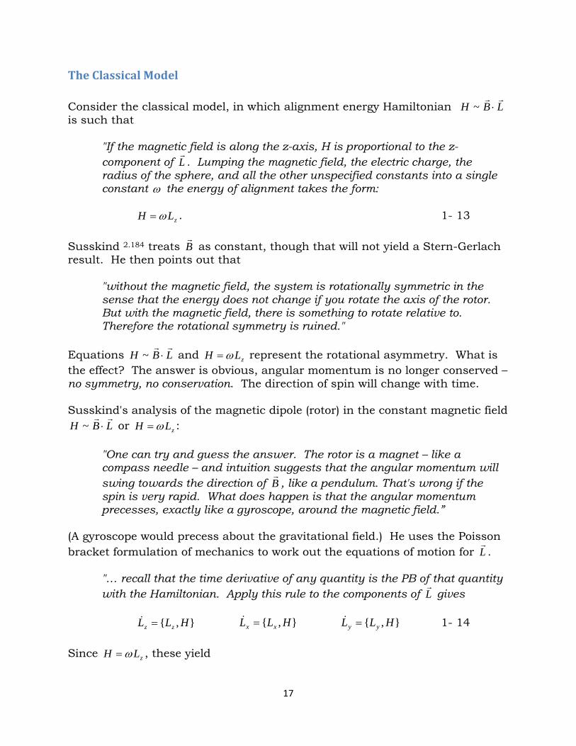
The Classical Model Consider the classical model, in which alignment energy Hamiltonian LBH

⋅~

is such that

"If the magnetic field is along the z-axis, H is proportional to the z-component of L

. Lumping the magnetic field, the electric charge, the

radius of the sphere, and all the other unspecified constants into a single constant ω the energy of alignment takes the form:

zLH ω= . 1- 13

Susskind 2.184 treats B

as constant, though that will not yield a Stern-Gerlach

result. He then points out that

"without the magnetic field, the system is rotationally symmetric in the sense that the energy does not change if you rotate the axis of the rotor. But with the magnetic field, there is something to rotate relative to. Therefore the rotational symmetry is ruined."

Equations LBH

⋅~ and zLH ω= represent the rotational asymmetry. What is

the effect? The answer is obvious, angular momentum is no longer conserved – no symmetry, no conservation. The direction of spin will change with time. Susskind's analysis of the magnetic dipole (rotor) in the constant magnetic field

LBH

⋅~ or zLH ω= :

"One can try and guess the answer. The rotor is a magnet – like a compass needle – and intuition suggests that the angular momentum will swing towards the direction of B

, like a pendulum. That's wrong if the

spin is very rapid. What does happen is that the angular momentum precesses, exactly like a gyroscope, around the magnetic field.”

(A gyroscope would precess about the gravitational field.) He uses the Poisson bracket formulation of mechanics to work out the equations of motion for L

.

"… recall that the time derivative of any quantity is the PB of that quantity with the Hamiltonian. Apply this rule to the components of L

gives

, HLL zz = , HLL xx =

, HLL yy = 1- 14 Since zLH ω= , these yield

17

, zzz LLL ω= , zxx LLL ω=

, zyy LLL ω= 1- 15 but zyx LLL =, so 0=zL , i.e., the z-component of L

does not change, and the

angle between B and L

does not change, "immediately precluding the idea that

L swings like a pendulum about B

." Cyclically permuting zyx LLL =, we have

yzx LLL −=,

xzy LLL +=, hence

yx LL ω−=

xy LL ω+= Susskind’s heuristic approach, assumes little initial physical knowledge. He first suggests that the magnetic moment swings in a plane like a pendulum about the B-field, with the angle between L

and B

changing periodically. He

then uses Poisson brackets to derive the equations of motion, finding that the z-component of L

is constant, hence the angle is constant.

"This is exactly the equation of a vector in the xy-plane rotating uniformly about the origin with angular frequency ω . In other words, L

precesses

about the magnetic field B

. Of this approach: "the magic of Poisson brackets allows us to solve the problem knowing very little other than that the Hamiltonian is proportional to LB

⋅ .”

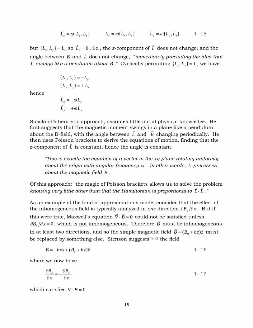
As an example of the kind of approximations made, consider that the effect of the inhomogeneous field is typically analyzed in one direction xBx ∂∂ . But if this were true, Maxwell's equation 0=⋅∇ B

could not be satisfied unless

0=∂∂ xBx , which is not inhomogeneous. Therefore B

must be inhomogeneous in at least two directions, and so the simple magnetic field zzbBB ˆ)( 0 +=

must

be replaced by something else. Stenson suggests 5.52 the field

zzbBxxbB ˆ)(ˆ 0 ++−=

1- 16 where we now have

zB

xB zx

∂∂

−=∂∂ 1- 17

which satisfies 0=⋅∇ B

.

18

This is the simplest magnetic field that satisfies the Stern-Gerlach conditions while also satisfying Maxwell's equations. Unfortunately this field blows up (grows without limit) away from the origin. Stenson notes that the simple 1D field zzbBB ˆ)( 0 +=

produces the correct results, and explains that it is the

"precession" that accounts for this, in the sense that in order to precess, the uniform field 0B must be much greater than the inhomogeneous field

|||| mogeneousinhomogeneousho BB

>> 1- 18 and hence

zBBbrB ˆ|||| 00 ≈⇒>>

That is, the inhomogeneity is ignored to first-order. So the 1D approximation is solved rigorously zBB ˆ0≈

for the homogeneous field, but then is subjectively

applied to a completely different problem5.57, with the field zzbBxxbB ˆ)(ˆ 0 ++−=

.

"this assumes that the interaction of these phenomena – the uniform and non-uniform parts of the field – is linear and can be naïvely superposed."

But Stenson shows that solving only the non-uniform part is non-trivial and suggests that more than just a linear interaction is occurring. Just because the expectation value time-averages to zero does not mean the measured value is zero, or even close to zero. From such considerations he concludes that

"At best the precession argument that is traditionally involved in thematic accounts of the Stern-Gerlach experiment disguises several interesting questions and at worst is completely invalid and inaccurate."

And he notes, as I have, that if this canonical quantum mechanical experiment is misinterpreted then there is also a possibility of other misinterpretations… For example, if precession is invalidly interpreted and the 2-D field yields a particle at a 45° angle from the location of the localized y-directed beam we would assume the particle felt an equal force in both x and z-directions, and would classically interpret such a result as a simultaneous measurement of both x and z-components of the magnetic moment. A quantum interpretation in which the strong 0B field (and hence precession) is removed leads to the possibility of simultaneous measurement of two components. Thus 5.59

"It is possible that our present understanding of the Uncertainty Principle only follows from our choice of field and not from the nature of the particles themselves."

19

Positivism or Realism? So the canonical Stern-Gerlach depends, for its quantum interpretation, on classical notions, specifically precession. This mixing of quantum and classical concepts is the basis of much confusion surrounding quantum mechanics. The fact that transverse spin components average to zero, based on the use of a magnetic field which clearly violates Maxwell's equations,5 “is an ad hoc assumption and has not been shown to easily follow from rigorous solutions." The prevalent view is that classical physics is a statistical approximation to quantum physics, which is assumed to be beyond human intuitive grasp. But why not assume that quantum physics is a measurement-induced approximat-ion to classical physics? Today it is primarily due to Bell's inequality and his theorem that local realism cannot produce quantum measurement results. Recall the two major views. In the positivist perspective, physical phenomena do not exist until observed. This is the basis of the Copenhagen interpretation and 'collapse of the wave function'. In the realist view, properties exist independently of the measurement, albeit are modified by measurement, i.e., the properties exist independently but their specific values do not. In the Copenhagen ( magical ) view, the particle is in a superposition of states and assumes a local reality on striking the detector. In the realist ( physical ) view, the particle has a real spin that exists and is detected by the detector. The Stern-Gerlach experiment serves to distinguish the positivist view from the realist view. The question is, does spin exist before measurement, or not.

"The precession interpretation makes sense only if spin actually exists; hence Copenhagen is inconsistent with the precession interpretation.”

One problem with realism is the lack of an expected continuous distribution. One problem with positivism is the idea of precession: what is precessing? If spin exists locally, then precessing make sense, and superposition is non-sense. If superposition is real, then spin does not exist locally, and precession is nonsense. Which is it? So Stern-Gerlach can be partitioned into two physical phenomena: precession (torque) in a homogeneous magnetic field and deflection (force) in an inhomo-geneous field. Stenson asked whether there is even any reason to apply the homogeneous field component.

20

"It's only purpose classically seems to be to induce precession about the direction of interest so that only components in that direction will be clearly observed."

But this becomes logically distorted such that

"In the old paradigm it was justified by our desire to measure only a single component of the magnetic moment, it has now become the justification for our [quantum] belief that measuring only one component is possible, via the Uncertainty Principle."

It seems incumbent on quantum mechanics to explain physical reality without this tortured logic. Or classical physicists must explain the success of quantum calculations and Bell's interpretation in terms of local realism.

Basic Physical Assumptions about Degrees of Freedom At issue in Stern-Gerlach experiments is quantization of spin. A non-uniform field exerts a force on a dipole, but a smeared distribution of particles passing through the field is expected if particles have random distributed spin vectors. Instead, we find +1 and -1. This is essentially unexplained… Brunner et al. 11 discuss an approach to ‘testing the dimension of an unknown physical system’, where dimension represents the number of degrees of free-dom of the system…

“… in contrast with the more usual approach in physics, in which, when constructing a theoretical model aiming at explaining some experimental data, the dimension of the system is a parameter that is defined a priori."

For example, a classical model of a magnetic dipole (rotor) has infinite degrees of freedom in that the dipole can point in any direction. But this would be expected to produce a continuous distribution in the output of the Stern-Gerlach experiment, which does not occur. Brunner et al. note that a model:

"...may or may not reproduce the experimental data. If the model fits the data, one can make a statement about the systems dimension. If it does however not work, nothing can be said, since, in principle, there could be a different model using the same dimension that could explain the data."

For example, the Bell model does not represent particle properties correctly; the data often violate Bell’s inequality. Perhaps a model with different dimension would reproduce the data. The problem of finding the dimensionality of classical and quantum systems is a black box scenario. Stern-Gerlach as black box is appropriate; EPR, based on it, has been a paradox for almost a century. Whereas the classical moment is a vector in 3-space, the 1D apparatus yields

21

only binary results, and Bell's analysis concludes local realism is incompatible with quantum theory. Could the a priori ‘dimension’ of his model be a problem? Bell makes no use of the inhomogeneous field required to obtain non-null results from Stern-Gerlach. When I mentioned this, Susskind said 12 "Oh, I'm sure Bell understood inhomogeneity." He may have understood it, but he does not model it. Bell and Susskind model the problem as essentially one-dimensional—that dimension being the angle θ between vectors L

and B

(or,

equivalently, the precession frequency.) They acknowledge this can change with absorption or emission of photons, but these are not believed to occur. The result: a two-state system whose physical components are mysterious and understood by no one, and the belief (that's all it is) that local realism is incompatible with quantum mechanics.

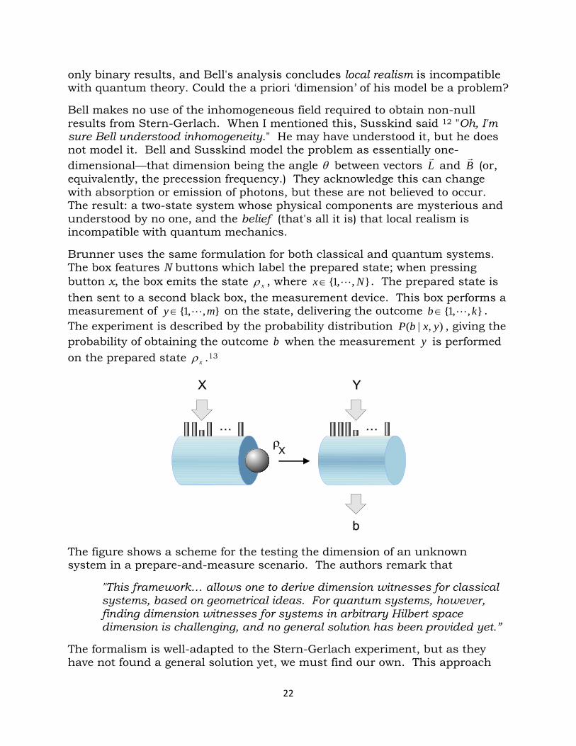
Brunner uses the same formulation for both classical and quantum systems. The box features N buttons which label the prepared state; when pressing button x, the box emits the state xρ , where ,,1 Nx ∈ . The prepared state is then sent to a second black box, the measurement device. This box performs a measurement of ,,1 my ∈ on the state, delivering the outcome ,,1 kb ∈ . The experiment is described by the probability distribution ),|( yxbP , giving the probability of obtaining the outcome b when the measurement y is performed on the prepared state xρ .13

The figure shows a scheme for the testing the dimension of an unknown system in a prepare-and-measure scenario. The authors remark that

"This framework… allows one to derive dimension witnesses for classical systems, based on geometrical ideas. For quantum systems, however, finding dimension witnesses for systems in arbitrary Hilbert space dimension is challenging, and no general solution has been provided yet.”

The formalism is well-adapted to the Stern-Gerlach experiment, but as they have not found a general solution yet, we must find our own. This approach

22

has focused attention on the fact that the Stern-Gerlach has been formulated a priori as a 1D problem, with that dimension identified as the potential energy of the precessing moment. Note that we have three 3-space vectors: dipole µ , field gradient dxdBBx =∇

,

and velocity dtxdv = . The dipole moves through the field gradient, with velocity

v . Since the particle is subject to a force, xx BF ∇⋅=µ , it accelerates the dipole

into a new region of the field, i.e., a different B-field; B

changes with time )( vxt ∆=∆ so, from the particle’s perspective, 0≠dtdB . But 0≠dxdB (as

Stern-Gerlach will not work with 0=dxdB ) and the velocity of the particle is not zero, so

xBvdtdx

dxdB

dtdB

∇⋅==

. 1- 19

Because the angular momentum is precessing, the L

vector is a complicated

function of time, and now we have a change in the B

vector with time, and a change in the velocity v of the atom with time, due to the force induced by the gradient, xx BF ∇⋅=

µ . We can attempt to solve for the changes in energy dtdH ,

due to the atom traveling through the gradient xB∇

, or we can ask how dtdH

can be made zero, i.e., energy be conserved. Does L change to accommodate

the changing B-field, and/or does energy exchange occur? As the precessing L

is constantly changing, this might seem to imply energy is

not conserved. But BL

⋅ is constant if B

is constant; if 0=dtdB and 0=dtdH , and the energy of the precessing dipole is conserved in a constant B-field. But with a constant B-field spins pass undeflected to the detector—a null result. What happens if the atom encounters a changing B-field? It’s no longer clear that 0=dtdH , so energy may not be conserved. This motivates investigation of whether a different dimension or number of degrees of freedom will reproduce the experimental data for what is, in most respects, an "unknown" system. In our case we contrast the one dimension )(xV versus )(xV and )(xT . The linear dimension v , through the inhomogeneous field, while understood to be the mechanism that actually produces the discrete outputs of the Stern-Gerlach experiment, is not actually modeled in the John Bell's analysis.

23

In his treatment of gauge and electromagnetic theory 2.207 Susskind says:

"If you look carefully at the (Hamiltonian with the vector potential A

)

−

−= ∑ )()(

21 xA

cepxA

cep

mH ii

iii 1- 20

you'll see something a little surprising. The combination

− )(xA

cep ii is

the mechanical velocity ivm . The Hamiltonian is nothing but

22mvH = In other words, its numerical value is the same as the naïve kinetic energy. This proves (among other things) that the energy is gauge invariant. Since it is conserved, the naïve kinetic energy is also conserved, as long as the magnetic field does not change with time."

But an inhomogeneous magnetic field exerting a force on a magnetic dipole traversing the field does change with time, and thus accelerates the dipole;

dtpdF = . The acceleration produces a change in kinetic energy. Or does it?

Does deflection in a magnetic field require energy?

The problem is the binary splitting of a beam of neutral atoms passing through a non-uniform magnetic field.

Does this splitting require energy or not? The 'bending of the trajectory' of the charged particle in a magnetic field, subject to Lorentz force )( BvqF

×= , does

not require energy, as |||| afterbefore vv = . The vector direction of the particle velocity is changed by the action of the magnetic field, but the magnitude || vv

= is not changed, hence kinetic energy 22mv is not changed. As Howard notes 6.44 in Nuclear Physics:

"Actually, there is no potential energy associated with the motion of a charged particle in a steady magnetic field, so that what appears here as a potential energy must in fact be a change in the kinetic energy of the moving charge associated with the establishment of the magnetic field."

But does the force of a non-uniform field on an uncharged magnetic dipole behave the same as a magnetic field on charge? The force equation )( BF

⋅∇= µ

14.326, 15, 9 implies that the force is zero if the energy is constant. But zero force gives a null result for Stern-Gerlach. And from the Lorentz force for a charged particle in a magnetic field, BvqF

×= , we see that the force is always perpend-

icular to the velocity, yielding zero work xdF ⋅ , while gradient force )( BF

⋅∇= µ

24

is independent of velocity, and thus can perform work. Therefore we conclude that energy changes when the dipole transits a non-uniform field. Thus, we expect the 22mv kinetic energy imparted by the field to represent real energy. But where does this energy come from? Susskind discusses 2.152 an electron in a changing electric field: In the capacitor experiment in which the energy of the electron is not conserved in the field inside a charging capacitor, he asks:

"What if we did the entire experiment now or later? The outcome, of course would be the same."

In other words, by expanding the model to take into account the switch and the charging battery,

"if we treated the entire collection as a single system, it would be time-translation invariant, and the total energy would be conserved."

The same logic applies to the Stern-Gerlach experiment; results are indepen-dent of whether we do the entire experiment now or later, so total energy is conserved. But what is the ‘entire system’ that we must analyze to achieve this? Susskind’s example of an electron in a changing electric field, needed to take into account the battery charging the capacitor. But there is no battery in the Stern-Gerlach circuit, only a non-uniform field shaped by a non-uniform magnet. So either the change in energy is globally-based, and energy must somehow re-arrange the microscopic spins in the magnetic material or the change in energy must be a local phenomena. When a physicist says that "energy is not conserved", he usually means that we must look further to find a system in which energy is conserved. We do have a local "battery" equivalent, in the sense that the energy of precession, LBH

⋅~ ,

is represented by the angle between the magnetic field B and the dipole L

. As

a local battery stores electric energy, a flywheel stores rotational energy. So if we desire to conserve total energy, 0=dH , we might assume that the energy is transferred from the 'local battery' (the flywheel ) to some other aspect of the local system. The two obvious aspects of energy are the precession energy of rotation and the (induced) kinetic energy. If the kinetic energy is maximized, then the precessional energy must be minimized, which occurs when there is no precession! This is true when 0≡θ , that is, the dipole is aligned with the magnetic field. Nassar and Miret-Artes 63 note that

"… in a system under observation, there are many degrees of freedom such that information can be lost in the couplings, which may account for dissipation."

25

Classical Analysis of Precessing in Stern-Gerlach The torque due to the magnetic dipole mis-alignment with the magnetic field attempts to align the dipole with the field. For constant dipole and a constant field the interaction energy )(~ BLB

⋅⋅µ is constant, and the dipole precesses.

A photon tuned to the right frequency can cause transition to a different angle (or precessing frequency). With no such tuned radiation in Stern-Gerlach, it is assumed that the particle simply continues to precess as it traverses the field. The classical precession, maintained at a given (Larmor) frequency, represents rotational inertia as proportional to 2mr . If the magnetic dipole has local energy (it does) then it has local equivalent mass, and this precession stores rotational energy, conceptually analogous to a flywheel. Recall that torque Fr

× has units

of work or energy, 2222 mvItml == ω , where I is moment of inertia 2~ mr , ω is frequency t1~ and v is linear velocity. So the torque attempts to align the dipole with the field, but the dynamics (in a constant field) lead to precession and conservation of energy B

⋅− µ . But we've

also seen that a dipole in an inhomogeneous field experiences force proportion-al to the gradient dxdB due to the fact that interaction energy B

⋅− µ changes

when B changes. The force acting on the particle accelerates it and increases

its kinetic energy 22mv . The question that seems to have been ignored is whether there is exchange of energy between these modes. If, as seems to be the case, precessional energy is assumed to be constant, 0θθ = , then the question of energy conservation arises. Based on the behavior of dipoles in 'extended' Stern-Gerlach devices, such as the Rabi-Ramsey molecular beam apparatus, and on Mansuripur's recent analysis of Maxwell's equations, we will assume that there is exchange of energy between the rotational mode and the linear motion modes. To analyze the situation we assume the particle has initial velocity )0,,0( yvv =

and initial

angle )ˆˆ(cos 1 B⋅= − µθ . The two-degrees-of-freedom Hamiltonian, )(xT and )(xV , is simply

BmvH

⋅−= µ22 1- 21 Energy = Linear + Rotational

Assume the magnetic field )(xB

is a function of x , such that gradient 0≠dxdBx . We know this will exert force in the x -direction, which will accelerate the particle in the x -direction, producing a velocity component xv , that is,

)0,,()0,,0( yxy vvvvv =→=

. 1- 22

26

Thus the situation is described by a force that wants to move the particle in the direction of the gradient and a torque that wants to align the particle with the field, and two corresponding modes of energy, i.e., degrees of freedom. And we know that if the radiation frequency is tuned correctly, the angle of precession θ will undergo change. As noted above, there are three vectors: the dipole µ which is changing due to precession, the field gradient xB∇

which is changing as we traverse the field,

and the velocity of the particle, which is being accelerated in the x -direction. One could attempt to solve for the dynamics of these three changing vectors in 3-space. Or we can require conservation of energy by demanding the Hamilton-ian be independent of time 0=dtdH .

⋅−== Bmv

dtd

dtdH µ

20

2

1- 23

( )Bdtd

dtpdv

⋅−⋅= µ

Since µ changes direction, and B changes magnitude, let us replace B

⋅− µ by

)cos(θk , where |||| Bk µ= is considered constant in the first approximation,

since, per Stenson, |||| mogeneousinhomogeneousho BB

>> . This assumption leads to

( ))(θfdtd

dtpdv =⋅

1- 24

which implies that the change in linear energy is equal to the change in rotational energy as measured by the angle of precession. The force acting to change the linear kinetic energy in a B-field gradient dxdBx is dxBdF

⋅= µ . If

µ and B

are orthogonal, the force is zero. If angle between µ and B

changes, the force changes, with maximum force when µ and B

are aligned, 0=θ .

So if the angle between µ and B

changes toward alignment the force increases until it reaches a maximum value at 0=θ . But if the energy is conserved, 0=H

( ) 0=⋅−⋅ Bdtd

dtpdv

µ 1- 25

( )Bdtd

dtpdv

⋅=⋅ µ

where dtpd is force F

and vF

⋅ is power dtdE= .

27

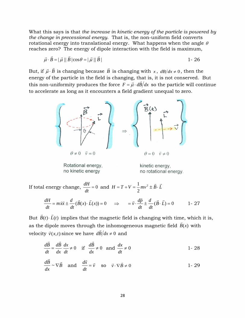
What this says is that the increase in kinetic energy of the particle is powered by the change in precessional energy. That is, the non-uniform field converts rotational energy into translational energy. What happens when the angle θ reaches zero? The energy of dipole interaction with the field is maximum,

||||cos|||| BBB µθµµ ==⋅ 1- 26

But, if B

⋅µ is changing because B

is changing with x , 0≠dxdB , then the energy of the particle in the field is changing, that is, it is not conserved. But this non-uniformity produces the force dxBdF

⋅= µ so the particle will continue

to accelerate as long as it encounters a field gradient unequal to zero.

If total energy change, 0=dt

dH and LBvmVTH

⋅±=+= 2

21

0))()(( =⋅±= xLxBdtdxxm

dtdH

⇒ 0)( =⋅±⋅= LBdtd

dtpdv

1- 27

But )()( tLtB

⋅ implies that the magnetic field is changing with time, which it is, as the dipole moves through the inhomogeneous magnetic field )(xB

with

velocity ),( txv since we have 0≠dxBd

and

0≠=dtdx

dxBd

dtBd

if 0≠dxBd

and 0≠dtdx 1- 28

BdxBd

∇~ and vdtxd

= so 0≠∇⋅ Bv 1- 29

28

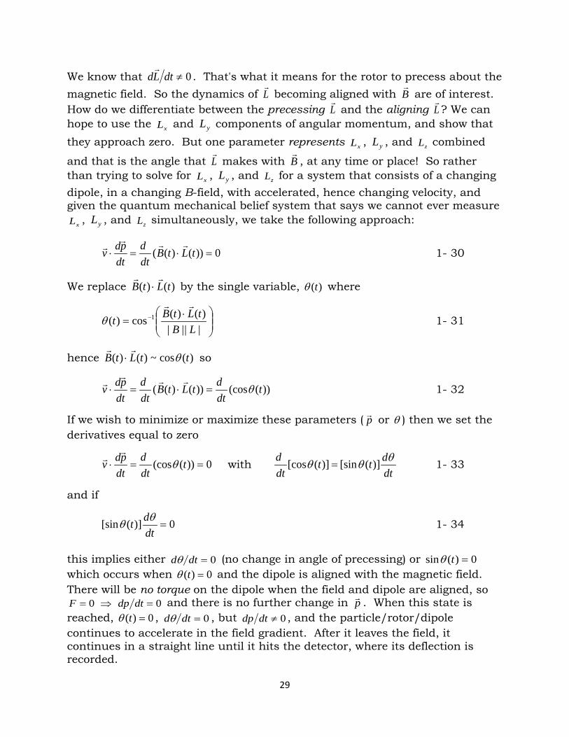
We know that 0≠dtLd

. That's what it means for the rotor to precess about the magnetic field. So the dynamics of L

becoming aligned with B

are of interest.

How do we differentiate between the precessing L and the aligning L

? We can

hope to use the xL and yL components of angular momentum, and show that they approach zero. But one parameter represents xL , yL , and zL combined

and that is the angle that L makes with B

, at any time or place! So rather

than trying to solve for xL , yL , and zL for a system that consists of a changing dipole, in a changing B-field, with accelerated, hence changing velocity, and given the quantum mechanical belief system that says we cannot ever measure

xL , yL , and zL simultaneously, we take the following approach:

0))()(( =⋅=⋅ tLtBdtd

dtpdv

1- 30

We replace )()( tLtB

⋅ by the single variable, )(tθ where

⋅= −

||||)()(cos)( 1

LBtLtBt

θ 1- 31

hence )(cos~)()( ttLtB θ

⋅ so

))((cos))()(( tdtdtLtB

dtd

dtpdv θ=⋅=⋅

1- 32 If we wish to minimize or maximize these parameters ( p or θ ) then we set the derivatives equal to zero

0))((cos ==⋅ tdtd

dtpdv θ

with

dtdtt

dtd θθθ )]([sin)]([cos = 1- 33

and if

0)]([sin =dtdt θθ 1- 34

this implies either 0=dtdθ (no change in angle of precessing) or 0)(sin =tθ which occurs when 0)( =tθ and the dipole is aligned with the magnetic field. There will be no torque on the dipole when the field and dipole are aligned, so

00 =⇒= dtdpF and there is no further change in p . When this state is reached, 0)( =tθ , 0=dtdθ , but 0≠dtdp , and the particle/rotor/dipole continues to accelerate in the field gradient. After it leaves the field, it continues in a straight line until it hits the detector, where its deflection is recorded.

29

Quantum Analysis of Stern-Gerlach

We have reviewed the classical formulation of a magnetic dipole precessing in a uniform field, and the quantum formulation which statistically supports such precessing. We discussed the non-uniform magnetic field—typically ignored or glossed over in Stern-Gerlach. Our analysis implies that exchange of energy between modes, or degrees of freedom, changes the picture. And the axiomatic, even iconic, place of Stern-Gerlach in quantum mechanics implies this novel treatment is significant. Other physicists seem to be coming to the same realization. Recently Navascues and Popescu 16 stated:

"Traditional descriptions of the measurement process and quantum mechanics typically overlook the energy exchange between the system under consideration and the measurement device carrying it."

They analyze the Bell-type CHSH experiment using photons, but we translate their statements straightforwardly into terms of Stern-Gerlach. Then we will examine their surprising and counterintuitive conclusion concerning quantum versus classical measurement, but first review a few facts about the energies:

Angular momentum

)1(|| += llL is quantized and conserved, but the energy

in the battery, BE

⋅= µ , is not quantized, as B

is a continuous variable. Consequently, whereas angular momentum L

can vary only by discrete values,

the energy )()( xBxE

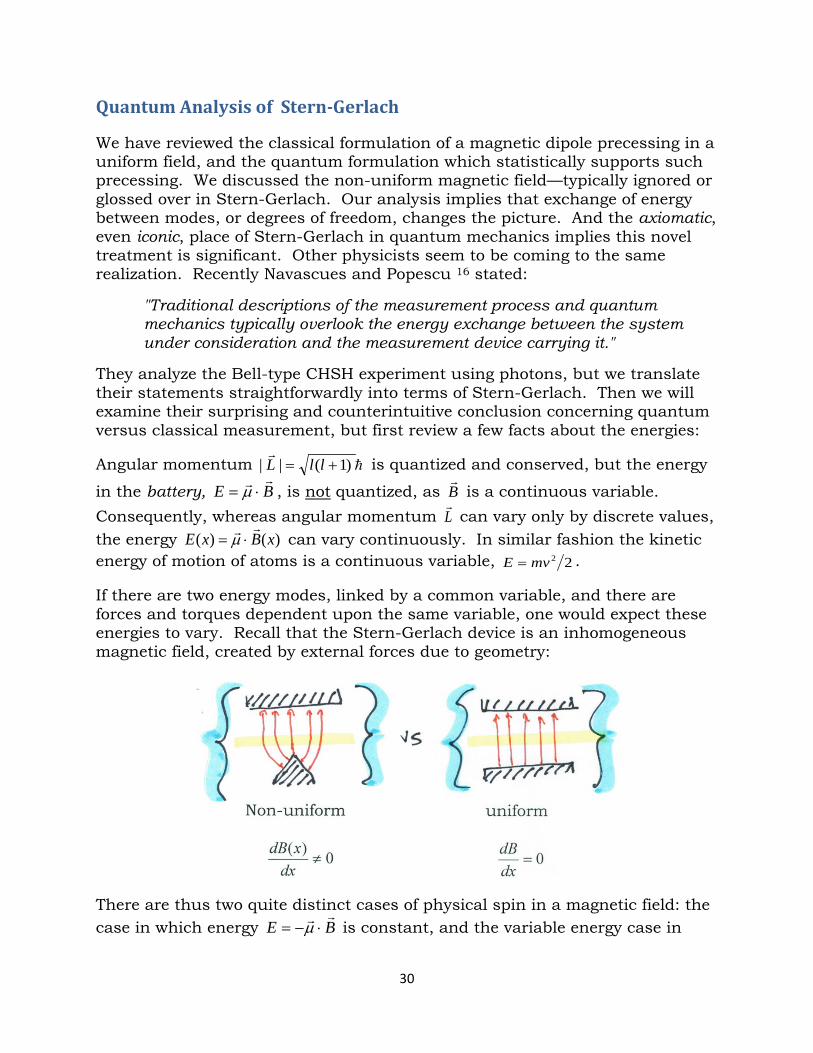
⋅= µ can vary continuously. In similar fashion the kinetic energy of motion of atoms is a continuous variable, 22mvE = . If there are two energy modes, linked by a common variable, and there are forces and torques dependent upon the same variable, one would expect these energies to vary. Recall that the Stern-Gerlach device is an inhomogeneous magnetic field, created by external forces due to geometry:

There are thus two quite distinct cases of physical spin in a magnetic field: the case in which energy BE

⋅−= µ is constant, and the variable energy case in

30

which )()( xBxE

⋅−= µ . In the first case energy is conserved, the dipole precesses and there is no deflection of the atom; a null result is obtained. In the second case the energy of both the system ( 22mv ) and the battery ( )(xB

⋅µ ) can vary.

Both the torque on the dipole (acting to align it with the field) and the force of the gradient, xB∇⋅

µ , depend on the alignment. So alignment angle θ is the common variable linking the two continuous energy modes. Conservation of energy implies that energy loss in one mode balances energy gain in the other mode. We impose energy conservation by requiring 0=dtdH . In this regard Navascues and Popescu ask16:

"What are the constraints imposed by conservation laws, when some form of exchange of conserved quantities is allowed?"

They state that

"… for any other conservative system, such as momentum and angular momentum, one can also consider an auxiliary system (i.e., a "battery") with which the conserved quantity can be exchanged, and the existence of such a battery will enlarge the class of possible measurements."

In the homogeneous case, the inability to exchange energy between the battery and system leads to null results—in line with the above statement—whereas with the exchange we get 1+ or 1− , obviously a larger class of measurements.

In the specific system they treat,

"… the target is the [laser] beam carrying the state )||( φφ ⟨⟩Atr , and the ancillary state )1|0|()21(| ⟩+⟩=+⟩ constitutes the battery."

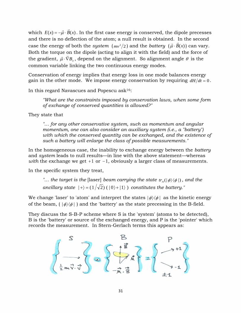
We change 'laser' to 'atom' and interpret the states || φφ ⟨⟩ as the kinetic energy of the beam, ( || φφ ⟨⟩ ) and the 'battery' as the state precessing in the B-field. They discuss the S-B-P scheme where S is the 'system' (atoms to be detected), B is the 'battery' or source of the exchanged energy, and P is the 'pointer' which records the measurement. In Stern-Gerlach terms this appears as:

31

Our system is the atom with kinetic energy, )(vE . Our battery is the precessing dipole with rotational energy— the flywheel or energy storage device. It is no wonder physicists find Stern-Gerlach confusing. They’ve believed they were measuring components of the magnetic dipole as a surrogate for spin. But whatever the original spin of the system, the configuration energy of the dipole is exchanged with the kinetic energy of linear modes and the spin is left in the aligned state which corresponds to the battery being ‘drained’. Conservation of energy through exchange between system and battery accounts for the 1± observed by the pointer. Navascues and Popescu state 16:

"Suppose now that we try to measure a target system S with Hamiltonian SH and assume that our measurement device has a battery with energy

operator ∑=j

jjBH πµ where jπ are orthogonal projection operators."

They base their analysis on laser beams and photons, not atomic beams and spin. In our Stern-Gerlach case the system Hamiltonian is

2|||| vvvxxH S =⋅=⟨⟩≡⟨⟩=φφ 1- 35

This is the usual mpH S 2ˆ~ 2 . We express their battery-energy operator as

aaHi

iij

jjB⋅=⇒= ∑∑ σσπµ 1- 36

where σ is the spin projection operator and a is Alice's setting. We see that

Ba

⋅⇔⋅ µσ . 1- 37

Energy stored in B

⋅µ is exchanged with SH such that conservation applies:

finalBSinitialBS HHHH )()( +=+ . 1- 38 These energy terms yield:

−

=

⋅−

∑∑

ii

ii BvmBvm ||||

2222 µµ . 1- 39

The |||| Bµ term represents the energy of the aligned final state, 0=θ . There is

no rotational energy of precession when µ is aligned with B

. If we choose coordinates so that the initial system state is in motion along the y-axis, then

)0,,0( yinit vv =

and the force of the gradient produces a displacement component of velocity along the x-axis, xv , that is included in the final energy:

32

||||)(2

)(2

222 BvvmBvmyxy

µµ −+=⋅− 1- 40

( )( ) 2

2cos1|||| xvmB =−⇒ θµ

( ~ 2θ )

This relation shows that the difference in the final aligned energy and the initial ‘battery’ energy, B

⋅− µ , is transferred to the motion of the particle.

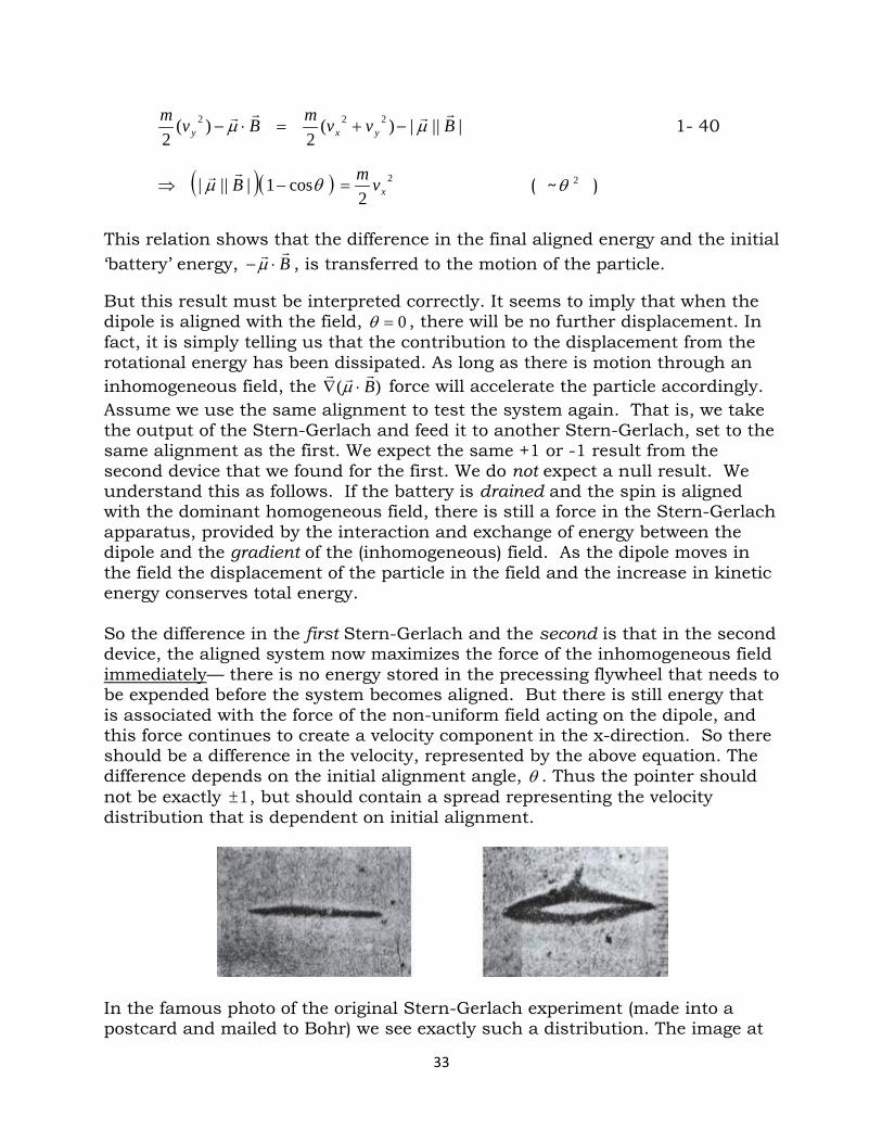
But this result must be interpreted correctly. It seems to imply that when the dipole is aligned with the field, 0=θ , there will be no further displacement. In fact, it is simply telling us that the contribution to the displacement from the rotational energy has been dissipated. As long as there is motion through an inhomogeneous field, the )( B

⋅∇ µ force will accelerate the particle accordingly.

Assume we use the same alignment to test the system again. That is, we take the output of the Stern-Gerlach and feed it to another Stern-Gerlach, set to the same alignment as the first. We expect the same +1 or -1 result from the second device that we found for the first. We do not expect a null result. We understand this as follows. If the battery is drained and the spin is aligned with the dominant homogeneous field, there is still a force in the Stern-Gerlach apparatus, provided by the interaction and exchange of energy between the dipole and the gradient of the (inhomogeneous) field. As the dipole moves in the field the displacement of the particle in the field and the increase in kinetic energy conserves total energy. So the difference in the first Stern-Gerlach and the second is that in the second device, the aligned system now maximizes the force of the inhomogeneous field immediately— there is no energy stored in the precessing flywheel that needs to be expended before the system becomes aligned. But there is still energy that is associated with the force of the non-uniform field acting on the dipole, and this force continues to create a velocity component in the x-direction. So there should be a difference in the velocity, represented by the above equation. The difference depends on the initial alignment angle, θ . Thus the pointer should not be exactly 1± , but should contain a spread representing the velocity distribution that is dependent on initial alignment.

In the famous photo of the original Stern-Gerlach experiment (made into a postcard and mailed to Bohr) we see exactly such a distribution. The image at

33

left is with no inhomogeneous field, while the image on the right is the quantum result that caused so much excitement, because a continuous distribution was expected for classical particles. The spread appears greater on the right than on the left. This has been ignored, and, I assume, attributed to a spread in the thermal velocity of the atoms, but we may be seeing the θ -dependent velocity contribution. Interestingly, the brass plaque at the Frankfurt institute that commemorates the experiment clearly shows the broad distribution. In their analysis of laser beams and photons Navascues and Popescu state16:

"If the Hamiltonians of the target and the battery do not have coincident energy gaps (i.e., if they are non-resonant) the presence of system B will not provide any advantages toward measuring or interacting with system S in a quantum way."

They immediately note that this is counterintuitive; they suggest a possible solution for this apparent paradox based on invoking or interacting with

"hidden continuous degrees of freedom". This remarkable "counterintuitive" observation tells us that the presence of the precessing dipole (battery) does not provide any advantage towards measuring or interacting with the atom in a quantum way! Instead, the continuous drain of energy from the precessing flywheel (as the torque aligns the dipole with the field) is exchanged with (added to) the velocity of the atom in a continuous, classical interaction, having nothing to do with "quantum spin".

More complex spin interactions While Stern-Gerlach describes a single spin in a field, there is support for change in precession from far more complex materials. For instance Kochan et al. report64 that in graphene "spin lifetimes of the Dirac electrons are expected to be long, on the order of microseconds, yet experiments find tenths of a nano-second. This has been the most outstanding puzzlement graphene spintronics.” Now both theory and experiment indicate that local magnetic moments in the graphene are the culprit. That is, magnetic impurities in graphene introduce local magnetic dipole fields that are in effect microscopic inhomogeneous magnetic fields that affect the orientation of the electron spin. In a somewhat similar vein 65 single electron spins and lattice vacancies have been shown to directly couple to nano-mechanical oscillations, yielding a mechanically driven spin transition, which can be mediated through electron-phonon coupling of the vacancy excited states. As Kalev 66 points out:

"An important distinction between classical and quantum measurement is that the latter implies an inevitable disturbance to the measured system."

34

Is Stern-Gerlach really a 'quantum' measurement?

If the physical process is as I have described it, the apparatus is the two-state device. The system is essentially a classical rotor/dipole. The quantum formu-lation is based on the "quantum measurement", which does not, as generally believed, actually measure components of the magnetic moment. It "quantizes" the moments by forcing them into alignment with the "measuring device" and then reports alignment or anti-alignment (+1 or -1) — mistakenly interpreted as a quantum characteristic of the particle. The experiment couples two different energies to a common variable implying that energy exchange occurs. We've seen the intuitive obviousness of this, but we next state it as a theorem. Please note that this does not remove the real quantized nature of the particle, the fact that the angular momentum is quantized in units of Planck's constant . That is a real phenomenon. But the 'qubit' nature of the particle is an artifact, imposed by the 1D "fishnet" apparatus. We will discuss the proper interpret-ation of the quantum formalism, but first we analyze 0≠dtdθ . In typical quantum mechanical books this is generally handled "quantum mechanically", which usually means "you won't understand how this can be, but I'll show you how to handle the quantum formalism of the problem.” How did the situation arise? Stern-Gerlach performed the experiment in 1922 while deBroglie particle/wave approach was circa 1925 and Heisenberg's and Schrödinger’s "incompatible" [at first] quantum formulations were in the 1925-26 timeframe. Many new and poorly understood aspects of physics were being digested, and the particle/wave aspect was especially difficult to understand. In addition, the spin ‘observed’ by Stern-Gerlach is not found in Schrödinger‘s wave function, postulated to contain all accessible information about a system.

Susskind's first Quantum Mechanics Lecture of Theoretical Minimum

As Stenson mentioned, Stern-Gerlach is more often used as a vehicle to carry quantum concepts than analyzed as the experiment that it is. Because his (free videos) lectures are popular worldwide I will focus on Leonard Susskind's introduction to quantum mechanics, beginning with his first lecture 17:

http://freevideolectures.com/Course/3151/The-Theoretical-Minimum-Quantum-Mechanics

Starting at minute 21 on the video Susskind defines a ‘system’ as a qubit, which when measured has heads or tails within a mathematical degree of freedom, σ . Then he shows three different notations for description of system: H ↑+= 1σ T ↓−= 1σ

35



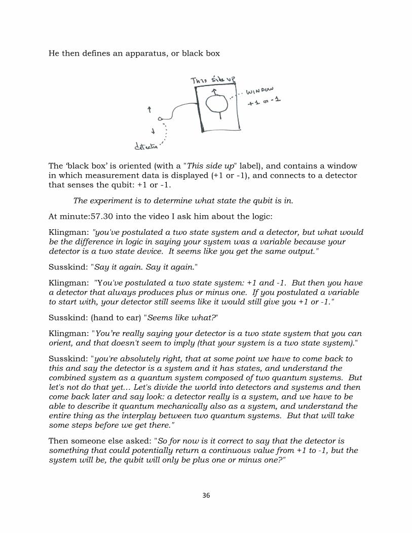
He then defines an apparatus, or black box

The ‘black box’ is oriented (with a "This side up" label), and contains a window in which measurement data is displayed (+1 or -1), and connects to a detector that senses the qubit: +1 or -1.

The experiment is to determine what state the qubit is in. At minute:57.30 into the video I ask him about the logic: Klingman: "you've postulated a two state system and a detector, but what would be the difference in logic in saying your system was a variable because your detector is a two state device. It seems like you get the same output." Susskind: "Say it again. Say it again." Klingman: "You've postulated a two state system: +1 and -1. But then you have a detector that always produces plus or minus one. If you postulated a variable to start with, your detector still seems like it would still give you +1 or -1."

Susskind: (hand to ear) "Seems like what?" Klingman: "You’re really saying your detector is a two state system that you can orient, and that doesn't seem to imply (that your system is a two state system)." Susskind: "you're absolutely right, that at some point we have to come back to this and say the detector is a system and it has states, and understand the combined system as a quantum system composed of two quantum systems. But let's not do that yet… Let's divide the world into detectors and systems and then come back later and say look: a detector really is a system, and we have to be able to describe it quantum mechanically also as a system, and understand the entire thing as the interplay between two quantum systems. But that will take some steps before we get there." Then someone else asked: "So for now is it correct to say that the detector is something that could potentially return a continuous value from +1 to -1, but the system will be, the qubit will only be plus one or minus one?"

36

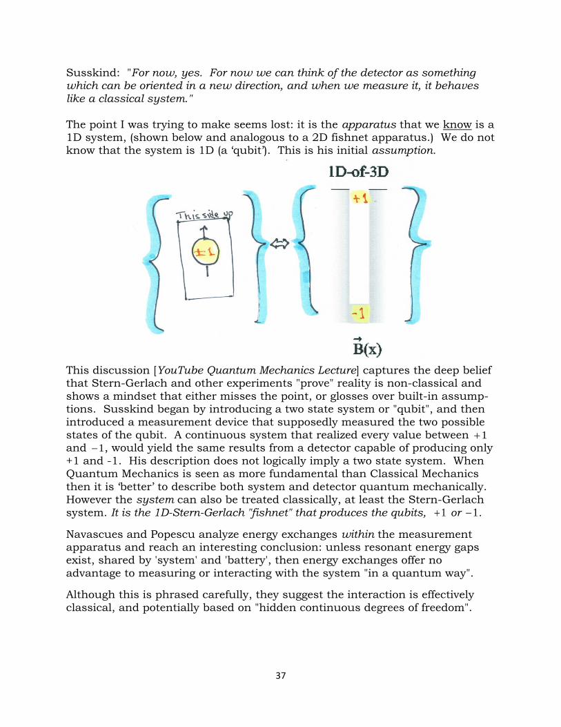
Susskind: "For now, yes. For now we can think of the detector as something which can be oriented in a new direction, and when we measure it, it behaves like a classical system." The point I was trying to make seems lost: it is the apparatus that we know is a 1D system, (shown below and analogous to a 2D fishnet apparatus.) We do not know that the system is 1D (a ‘qubit’). This is his initial assumption.

This discussion [YouTube Quantum Mechanics Lecture] captures the deep belief that Stern-Gerlach and other experiments "prove" reality is non-classical and shows a mindset that either misses the point, or glosses over built-in assump-tions. Susskind began by introducing a two state system or "qubit", and then introduced a measurement device that supposedly measured the two possible states of the qubit. A continuous system that realized every value between 1+and 1− , would yield the same results from a detector capable of producing only +1 and -1. His description does not logically imply a two state system. When Quantum Mechanics is seen as more fundamental than Classical Mechanics then it is ‘better’ to describe both system and detector quantum mechanically. However the system can also be treated classically, at least the Stern-Gerlach system. It is the 1D-Stern-Gerlach "fishnet" that produces the qubits, 1+ or 1− .

Navascues and Popescu analyze energy exchanges within the measurement apparatus and reach an interesting conclusion: unless resonant energy gaps exist, shared by 'system' and 'battery', then energy exchanges offer no advantage to measuring or interacting with the system "in a quantum way". Although this is phrased carefully, they suggest the interaction is effectively classical, and potentially based on "hidden continuous degrees of freedom".

37

An Energy Exchange Theorem We have discussed a process whereby energy is exchanged between two modes in the operation of the apparatus. Although that seems likely, based on being coupled to a common variable, it both depends on the variable changing and upon the energy exchange occurring. We now desire to put this process on firmer ground, and do so by stating and proving the following theorem:

The Energy Exchange Theorem: Given the existence of a system with two modes of energy coupled to one variable, conservation of energy implies energy exchange between the modes.

We prove by contradiction. Assume no exchange occurs when the common variable (call it θ ) changes — energy 1E of mode 1 and 2E of mode 2 are independent of each other: ))(()( 21 θθ EfE ≠ . But our theorem says that each mode is coupled to θ , so

θθ

θ dddEE 1

1 )( =∆ and θθ

θ dddEE 2

2 )( =∆ 1- 41

And conservation of energy implies the Hamiltonian is time independent:

0=dt

dH 02121 =

+=+⇒

dtd

ddE

dtd

ddE

dtdE

dtdE θ

θθ

θ 1- 42

therefore

021 =

+

dtd

ddE

ddE θ

θθ 1- 43

If 0≠dtdθ then this implies

θθ d

dEddE 21 −= 1- 44

which contradicts our assumption. Q.E.D. We look next at the evidence for 0≠dtdθ .

38

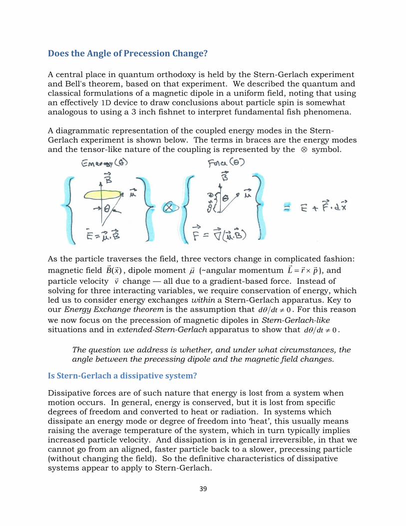
Does the Angle of Precession Change? A central place in quantum orthodoxy is held by the Stern-Gerlach experiment and Bell's theorem, based on that experiment. We described the quantum and classical formulations of a magnetic dipole in a uniform field, noting that using an effectively 1D device to draw conclusions about particle spin is somewhat analogous to using a 3 inch fishnet to interpret fundamental fish phenomena. A diagrammatic representation of the coupled energy modes in the Stern-Gerlach experiment is shown below. The terms in braces are the energy modes and the tensor-like nature of the coupling is represented by the ⊗ symbol.

As the particle traverses the field, three vectors change in complicated fashion: magnetic field )(xB

, dipole moment µ (~angular momentum prL ×= ), and

particle velocity v change — all due to a gradient-based force. Instead of solving for three interacting variables, we require conservation of energy, which led us to consider energy exchanges within a Stern-Gerlach apparatus. Key to our Energy Exchange theorem is the assumption that 0≠dtdθ . For this reason we now focus on the precession of magnetic dipoles in Stern-Gerlach-like situations and in extended-Stern-Gerlach apparatus to show that 0≠dtdθ .

The question we address is whether, and under what circumstances, the angle between the precessing dipole and the magnetic field changes.

Is Stern-Gerlach a dissipative system? Dissipative forces are of such nature that energy is lost from a system when motion occurs. In general, energy is conserved, but it is lost from specific degrees of freedom and converted to heat or radiation. In systems which dissipate an energy mode or degree of freedom into ‘heat’, this usually means raising the average temperature of the system, which in turn typically implies increased particle velocity. And dissipation is in general irreversible, in that we cannot go from an aligned, faster particle back to a slower, precessing particle (without changing the field). So the definitive characteristics of dissipative systems appear to apply to Stern-Gerlach.

39

Assume that the energy of precession is converted into the energy of linear motion. In the non-uniform field the force is specified as )( BF

⋅∇= µ , or its

simpler approximation xBF ∆⋅∆= )(µ . If we multiply by tt ∆∆ we obtain

( ) ( ) ( )BdtdvFB

txtB

xF

⋅=⋅⇒⋅

∆∆

∆∆

⇒⋅∆∆

= µµµ 1- 45

Since B

⋅µ is the precessing energy we see that the change in such energy with time is proportional to the velocity of the particle in a non-uniform field times the measure of non-uniformity—the gradient. So the key criteria for dissipative system seem to be met. Of course if we exchange B

⋅µ for 2vvm

⋅ we obtain:

( ) Fmadtdvmvm

tdd

vB

tdd

vF ===

⇒⋅=

211 2µ 1- 46

This is expected; nevertheless, dimensional checks are good. Other examples exist involving exchanges between two separate energy modes or degrees of freedom that interact and influence each other. Vibronic coupling is a case of non-adiabatic coupling or derivative coupling in a molecule based on interactions between electronic and nuclear vibrational motion. Although Susskind is unsure about what is precessing, he implies in lectures that the precessing moment will continue to precess unless it emits or absorbs a photon. An apparent consensus of physicists is that,

with no absorption or emission of photons to deliver or carry away angular momentum and energy, a dipole moment will continue to precess and θ will be preserved.

How likely is it that the dipole will emit a photon? Is magnetic dipole radiation even detectable? Ivanov and Karlovets18 note that electromagnetic radiation can be produced by neutral particles carrying magnetic moments, but the contribution of the magnetic moment to any kind of polarization radiation (in the presence of a medium) has never been detected. Experimental observation of the influence of the magnetic moment in electromagnetic radiation is very scarce and limited to very few cases of spin-induced effects in bremstrahlung. Absorption of electromagnetic radiation by magnetic moments is, however, quite common. Some experiments deal with individual (charged) particles caught in a Penning trap and subject to oscillating fields which can ‘flip’ the spin of individual particles. Most such traps use a strong homogeneous field and a strong inhomogeneous electric field; a recent version is such that 19,20:

"A strong magnetic field inhomogeneity couples the proton’s spin direction to the frequency with which the proton oscillates along the direction of the trap's magnetic field. This frequency is measured to monitor the single-proton spin flips, which are induced by an external radiofrequency field."

40

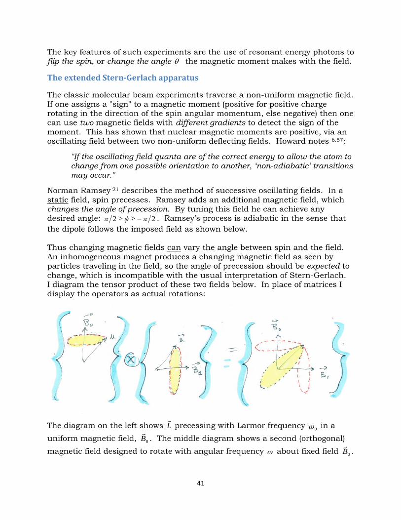
The key features of such experiments are the use of resonant energy photons to flip the spin, or change the angle θ the magnetic moment makes with the field.

The extended Stern-Gerlach apparatus The classic molecular beam experiments traverse a non-uniform magnetic field. If one assigns a "sign" to a magnetic moment (positive for positive charge rotating in the direction of the spin angular momentum, else negative) then one can use two magnetic fields with different gradients to detect the sign of the moment. This has shown that nuclear magnetic moments are positive, via an oscillating field between two non-uniform deflecting fields. Howard notes 6.57:

"If the oscillating field quanta are of the correct energy to allow the atom to change from one possible orientation to another, ‘non-adiabatic’ transitions may occur."

Norman Ramsey 21 describes the method of successive oscillating fields. In a static field, spin precesses. Ramsey adds an additional magnetic field, which changes the angle of precession. By tuning this field he can achieve any desired angle: 22 πφπ −≥≥ . Ramsey’s process is adiabatic in the sense that the dipole follows the imposed field as shown below. Thus changing magnetic fields can vary the angle between spin and the field. An inhomogeneous magnet produces a changing magnetic field as seen by particles traveling in the field, so the angle of precession should be expected to change, which is incompatible with the usual interpretation of Stern-Gerlach. I diagram the tensor product of these two fields below. In place of matrices I display the operators as actual rotations:

The diagram on the left shows L

precessing with Larmor frequency 0ω in a

uniform magnetic field, 0B

. The middle diagram shows a second (orthogonal) magnetic field designed to rotate with angular frequency ω about fixed field 0B

.

41

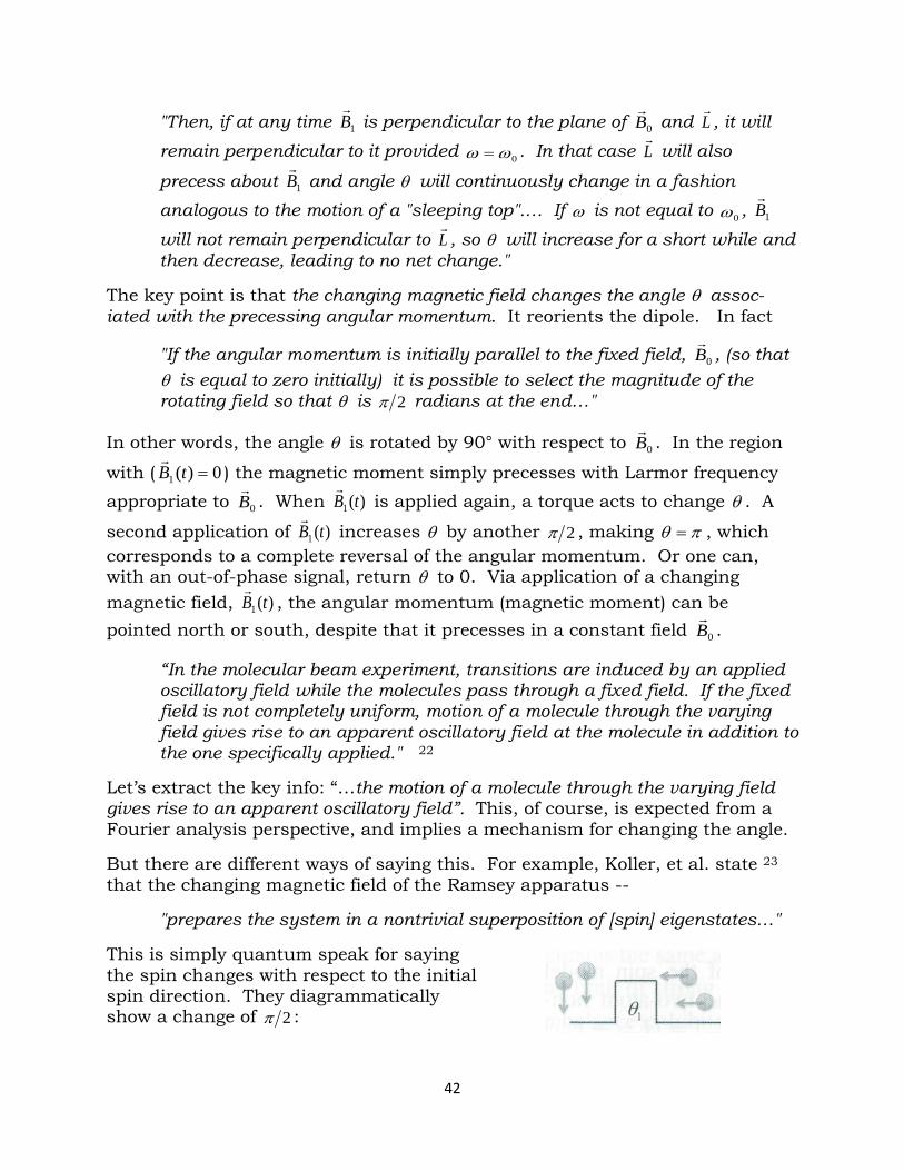
"Then, if at any time 1B

is perpendicular to the plane of 0B

and L, it will

remain perpendicular to it provided 0ωω = . In that case L will also

precess about 1B

and angle θ will continuously change in a fashion analogous to the motion of a "sleeping top".… If ω is not equal to 0ω , 1B

will not remain perpendicular to L, so θ will increase for a short while and

then decrease, leading to no net change."

The key point is that the changing magnetic field changes the angle θ assoc-iated with the precessing angular momentum. It reorients the dipole. In fact

"If the angular momentum is initially parallel to the fixed field, 0B

, (so that θ is equal to zero initially) it is possible to select the magnitude of the rotating field so that θ is 2π radians at the end…"

In other words, the angle θ is rotated by 90° with respect to 0B

. In the region

with ( 0)(1 =tB

) the magnetic moment simply precesses with Larmor frequency appropriate to 0B

. When )(1 tB

is applied again, a torque acts to change θ . A

second application of )(1 tB

increases θ by another 2π , making πθ = , which corresponds to a complete reversal of the angular momentum. Or one can, with an out-of-phase signal, return θ to 0. Via application of a changing magnetic field, )(1 tB

, the angular momentum (magnetic moment) can be

pointed north or south, despite that it precesses in a constant field 0B

.

“In the molecular beam experiment, transitions are induced by an applied oscillatory field while the molecules pass through a fixed field. If the fixed field is not completely uniform, motion of a molecule through the varying field gives rise to an apparent oscillatory field at the molecule in addition to the one specifically applied." 22

Let’s extract the key info: “…the motion of a molecule through the varying field gives rise to an apparent oscillatory field”. This, of course, is expected from a Fourier analysis perspective, and implies a mechanism for changing the angle. But there are different ways of saying this. For example, Koller, et al. state 23 that the changing magnetic field of the Ramsey apparatus --

"prepares the system in a nontrivial superposition of [spin] eigenstates…" This is simply quantum speak for saying the spin changes with respect to the initial spin direction. They diagrammatically show a change of 2π :

42

There is thus no question that the spin direction changes due to the change in magnetic field through which the spin passes. The question is one of timing, i.e., adiabatic or non-adiabatic change. Ramsey describes using an inhomo-geneous field in the oscillatory field regions, beginning far from resonance:

“When the resonance condition is slowly approached, the magnetic moment that was initially aligned parallel to 0H

will adiabatically follow

the effective magnetic field on a coordinate system rotating with 1H

until… the moment is parallel to 1H

and therefore at angle 2πφ = . The moment

precesses in the intermediate region and then the oscillatory field applied shifts the moment from parallel to 1H

to parallel to 0H

.”

Keywords are slowly and adiabatically. The adiabatic theorem 56:

"A physical system remains in its instantaneous eigenstate if a given perturbation is acting on it slowly enough and if there is a gap between the eigenvalue and the rest of the Hamiltonian's spectrum."

The key word here is "and", that is, "and if there is a gap between the eigen-values and the rest of the Hamiltonian's spectrum." But if the atom’s Hamiltonian is

BLmvH ⋅+=

22 , 1- 47 then there is no gap, as the kinetic energy of the particle in the inhomogeneous field is a continuum, not a discrete eigenspectrum. Therefore the system has time to adapt its configuration and has a mechanism of energy exchange:

)2()( 2mvdtdBL

dtd

⇒⋅

. 1- 48

In a static field the Hamiltonian is BL

⋅~ and there is torque, but no force to change the particle’s linear momentum. The quantum nature of angular momentum does produce a gap: )1( += llL , mLz = and this gap prevents the adiabatic change in state, so spin precesses with no change in BL

⋅ , hence no

change in θ . In a changing field angular momentum L’s magnitude does not

change, only its direction. But angular momentum associated with precession does vanish if the dipole aligns with the field. But if the bending of the particle path represents an increase in the angular momentum represented by

prL ×=′ then angular momentum is conserved. Detailed calculations should

show this. We note that a very relevant paper by Koller, et al. states 23

43

"In many theoretical treatments, key to understanding the dynamics has been to assume the external (motional) degrees of freedom are decoupled from the pseudo-spin degrees of freedom. Determining the validity of this approximation – known as the spin model approximation – has not been addressed in detail."

I find it amazing that such a key assumption "has not been addressed in detail" in the 92 years since Stern-Gerlach performed their axiomatic experiment that served to 'explain' many quantum mechanical concepts, and was used by Bell to banish local realism. Perhaps it is time to address the issue that:

"The external degrees of freedom can affect the spin dynamics in a non-trivial way… A great simplification could be gained if it were possible to decouple the motional and spin degrees of freedom…"

As a vehicle they focus on a 'pure spin model' description of Ramsey spectro-scopy, by performing exact calculations on fermions confined in quasi-1D and quasi-2D harmonic traps. While this facilitates calculations, it introduces the "gap" we discussed "between the eigenvalue and the rest of the Hamiltonian's spectrum". That is, by confining the particles in a quantum oscillator potential, they violate the conditions of our Energy Exchange Theorem. Nevertheless they say that their two body calculations are

"…a first step towards understanding the interplay between spin and particle motion in generic many-body ensembles."

Although their laser-irradiated trap-confined fermions are not the best model of our Stern-Gerlach system, they state that:

"In one dimension the spin model treatment breaks down for dark times on the order of the inverse interaction strength, and for strong interactions. In two dimensions we find an effective spin model… whose dynamics can be quite different from those predicted by spin model treatment."

In other words the motional and spin degrees of freedom are coupled. But this brings the equations of coupled fields into the picture. And these are Maxwell’s equations. Recently Masud Mansuripur claimed that situations that involve exchange of linear and angular momentum require using specific terms.

44

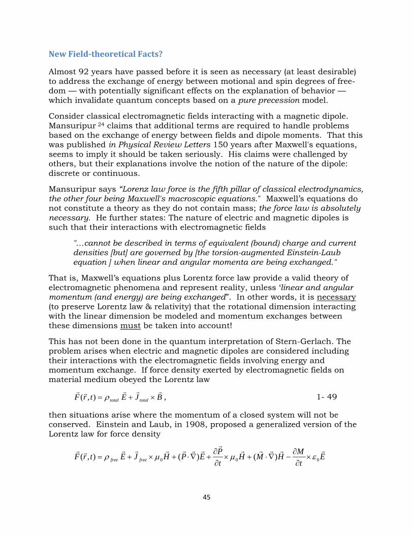
New Field-theoretical Facts? Almost 92 years have passed before it is seen as necessary (at least desirable) to address the exchange of energy between motional and spin degrees of free-dom — with potentially significant effects on the explanation of behavior — which invalidate quantum concepts based on a pure precession model. Consider classical electromagnetic fields interacting with a magnetic dipole. Mansuripur 24 claims that additional terms are required to handle problems based on the exchange of energy between fields and dipole moments. That this was published in Physical Review Letters 150 years after Maxwell's equations, seems to imply it should be taken seriously. His claims were challenged by others, but their explanations involve the notion of the nature of the dipole: discrete or continuous. Mansuripur says “Lorenz law force is the fifth pillar of classical electrodynamics, the other four being Maxwell's macroscopic equations." Maxwell’s equations do not constitute a theory as they do not contain mass; the force law is absolutely necessary. He further states: The nature of electric and magnetic dipoles is such that their interactions with electromagnetic fields

"…cannot be described in terms of equivalent (bound) charge and current densities [but] are governed by [the torsion-augmented Einstein-Laub equation ] when linear and angular momenta are being exchanged."

That is, Maxwell’s equations plus Lorentz force law provide a valid theory of electromagnetic phenomena and represent reality, unless ‘linear and angular momentum (and energy) are being exchanged”. In other words, it is necessary (to preserve Lorentz law & relativity) that the rotational dimension interacting with the linear dimension be modeled and momentum exchanges between these dimensions must be taken into account! This has not been done in the quantum interpretation of Stern-Gerlach. The problem arises when electric and magnetic dipoles are considered including their interactions with the electromagnetic fields involving energy and momentum exchange. If force density exerted by electromagnetic fields on material medium obeyed the Lorentz law

BJEtrF totaltotal

×+= ρ),( , 1- 49

then situations arise where the momentum of a closed system will not be conserved. Einstein and Laub, in 1908, proposed a generalized version of the Lorentz law for force density

Et

MHMHtPEPHJEtrF freefree

000 )()(),( εµµρ ×

∂∂

−∇⋅+×∂∂

+∇⋅+×+=

45

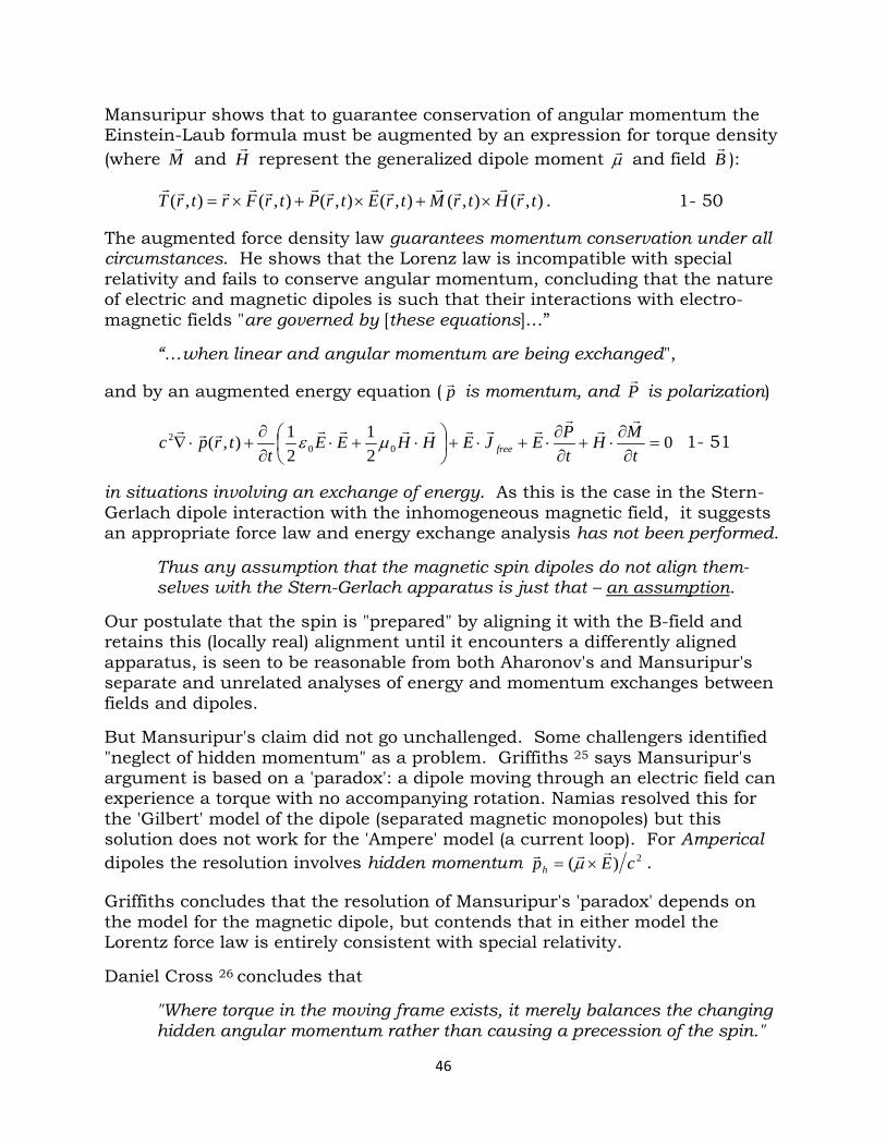
Mansuripur shows that to guarantee conservation of angular momentum the Einstein-Laub formula must be augmented by an expression for torque density (where M

and H

represent the generalized dipole moment µ and field B

):

),(),(),(),(),(),( trHtrMtrEtrPtrFrtrT ×+×+×= . 1- 50

The augmented force density law guarantees momentum conservation under all circumstances. He shows that the Lorenz law is incompatible with special relativity and fails to conserve angular momentum, concluding that the nature of electric and magnetic dipoles is such that their interactions with electro-magnetic fields "are governed by [these equations]…”

“…when linear and angular momentum are being exchanged",

and by an augmented energy equation ( p is momentum, and P

is polarization)

021

21),( 00

2 =∂∂⋅+

∂∂⋅+⋅+

⋅+⋅

∂∂

+⋅∇t

MHtPEJEHHEE

ttrpc free

µε 1- 51

in situations involving an exchange of energy. As this is the case in the Stern-Gerlach dipole interaction with the inhomogeneous magnetic field, it suggests an appropriate force law and energy exchange analysis has not been performed.

Thus any assumption that the magnetic spin dipoles do not align them-selves with the Stern-Gerlach apparatus is just that – an assumption.

Our postulate that the spin is "prepared" by aligning it with the B-field and retains this (locally real) alignment until it encounters a differently aligned apparatus, is seen to be reasonable from both Aharonov's and Mansuripur's separate and unrelated analyses of energy and momentum exchanges between fields and dipoles. But Mansuripur's claim did not go unchallenged. Some challengers identified "neglect of hidden momentum" as a problem. Griffiths 25 says Mansuripur's argument is based on a 'paradox': a dipole moving through an electric field can experience a torque with no accompanying rotation. Namias resolved this for the 'Gilbert' model of the dipole (separated magnetic monopoles) but this solution does not work for the 'Ampere' model (a current loop). For Amperical dipoles the resolution involves hidden momentum 2)( cEph

×= µ .

Griffiths concludes that the resolution of Mansuripur's 'paradox' depends on the model for the magnetic dipole, but contends that in either model the Lorentz force law is entirely consistent with special relativity. Daniel Cross 26 concludes that

"Where torque in the moving frame exists, it merely balances the changing hidden angular momentum rather than causing a precession of the spin."

46

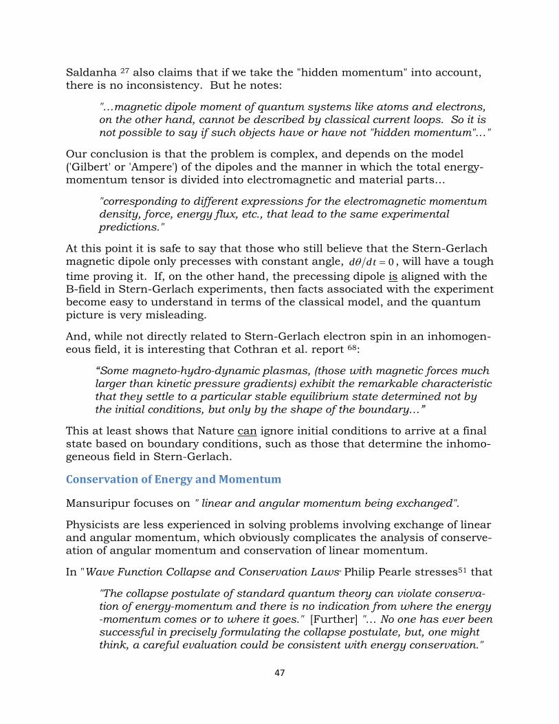
Saldanha 27 also claims that if we take the "hidden momentum" into account, there is no inconsistency. But he notes:

"…magnetic dipole moment of quantum systems like atoms and electrons, on the other hand, cannot be described by classical current loops. So it is not possible to say if such objects have or have not "hidden momentum"…"

Our conclusion is that the problem is complex, and depends on the model ('Gilbert' or 'Ampere') of the dipoles and the manner in which the total energy-momentum tensor is divided into electromagnetic and material parts…

"corresponding to different expressions for the electromagnetic momentum density, force, energy flux, etc., that lead to the same experimental predictions."

At this point it is safe to say that those who still believe that the Stern-Gerlach magnetic dipole only precesses with constant angle, 0=tddθ , will have a tough time proving it. If, on the other hand, the precessing dipole is aligned with the B-field in Stern-Gerlach experiments, then facts associated with the experiment become easy to understand in terms of the classical model, and the quantum picture is very misleading. And, while not directly related to Stern-Gerlach electron spin in an inhomogen-eous field, it is interesting that Cothran et al. report 68:

“Some magneto-hydro-dynamic plasmas, (those with magnetic forces much larger than kinetic pressure gradients) exhibit the remarkable characteristic that they settle to a particular stable equilibrium state determined not by the initial conditions, but only by the shape of the boundary…”

This at least shows that Nature can ignore initial conditions to arrive at a final state based on boundary conditions, such as those that determine the inhomo-geneous field in Stern-Gerlach.

Conservation of Energy and Momentum Mansuripur focuses on " linear and angular momentum being exchanged". Physicists are less experienced in solving problems involving exchange of linear and angular momentum, which obviously complicates the analysis of conserve-ation of angular momentum and conservation of linear momentum. In "Wave Function Collapse and Conservation Laws" Philip Pearle stresses51 that

"The collapse postulate of standard quantum theory can violate conserva-tion of energy-momentum and there is no indication from where the energy -momentum comes or to where it goes." [Further] "… No one has ever been successful in precisely formulating the collapse postulate, but, one might think, a careful evaluation could be consistent with energy conservation."

47

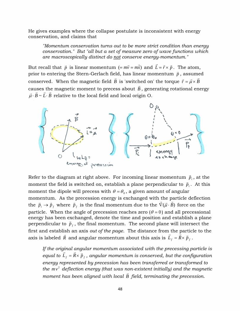
He gives examples where the collapse postulate is inconsistent with energy conservation, and claims that

"Momentum conservation turns out to be more strict condition than energy conservation." But "all but a set of measure zero of wave functions which are macroscopically distinct do not conserve energy-momentum."

But recall that p is linear momentum )( xmvm == and prL

×= . The atom, prior to entering the Stern-Gerlach field, has linear momentum p , assumed conserved. When the magnetic field B

is 'switched on' the torque B

×= µτ

causes the magnetic moment to precess about B

, generating rotational energy BLB

⋅⋅ ~µ relative to the local field and local origin O.

Refer to the diagram at right above. For incoming linear momentum ip , at the moment the field is switched on, establish a plane perpendicular to ip . At this moment the dipole will precess with 0θθ = , a given amount of angular momentum. As the precession energy is exchanged with the particle deflection the fi pp

→ where fp is the final momentum due to the )( B

⋅∇ µ force on the particle. When the angle of precession reaches zero ( 0=θ ) and all precessional energy has been exchanged, denote the time and position and establish a plane perpendicular to fp , the final momentum. The second plane will intersect the first and establish an axis out of the page. The distance from the particle to the axis is labeled R

and angular momentum about this axis is ff pRL

×= .

If the original angular momentum associated with the precessing particle is equal to ff pRL

×= , angular momentum is conserved, but the configuration energy represented by precession has been transferred or transformed to the 2vm deflection energy (that was non-existent initially) and the magnetic moment has been aligned with local B

field, terminating the precession.

48

Quantum caveat

Some experiments show light exhibits the properties of waves while others show it exhibits properties of particles, so Stenson notes that we can use well-defined particle concepts of position, speed, mass, trajectories and force but also wave fronts, interference, crests, troughs, frequency and amplitude:5.16

"We have effectively doubled the space in which we describe quantum mechanics by doubling the number of concepts that can be applied to it… the reverse of the vector… in which we choose a mathematical represent-ation so as to reduce the dimensionality of the problem."

But "the implications and emphasis of the representation become confused with those of the original phenomena."

Consider use of a classical angular momentum vector to represent spin, versus infinite plane wave solutions to Schrödinger’s equation for the same problem. Stenson begins with a quantum mechanical solution5.80 to the appropriate Hamiltonian — describing the atomic beam as an infinite plane wave. Then he formulates the problem as Clifford algebra spinors, and in the Schrödinger, Heisenberg, and Dirac pictures 5.87. Each approach to solving the inhomo-geneous Stern-Gerlach problem involves approximating and assuming— preventing Stenson from drawing solid conclusions. Instead it reinforces that:

"While representations are necessary in order for rational communication and comprehension they also necessarily alter the perceived behavior of the phenomena they represent."

For example, precession is vital to standard descriptions of the Stern-Gerlach effect, due to its averaging away incompatible components. Stenson concludes that use of several representations is interesting not so much for the specific knowledge but that there is absolute knowledge—what I would term knowledge of reality —so "shut up and calculate" is not a philosoph-ically satisfactory attitude. Stenson: "It works’ should only serve as temporary justification for pursuing knowledge and not as a permanent replacement."

Quantum mechanics is inconsistent, with one foot in classical description and the other in axiomatic representation. Incompatibilities and impossibilities from John Bell's theorem are based on quantum mechanical representation and attendant assumptions. Can these incompatibilities be resolved and the classical model sought by Bell be made compatible with quantum mechanics? Angular momentum and the wave nature of propagating particles are two such different aspects of reality best represented differently. Both are susceptible to classical explanation. We will distinguish between inherent wave properties of particles with linear momentum and the different nature of "spin".

49

Bell’s Theorem David Bohm said 57 in 1952:

"The usual interpretation of the quantum theory requires us to give up the possibility of even conceiving precisely what might determine the behavior of an individual system at the quantum level, without providing adequate proof that such a renunciation is necessary. The usual interpretation is admittedly consistent; but [this] does not exclude the possibility of other equally consistent interpretations…"

John Bell in 1964 claimed 1.14 to provide adequate proof. He begins:

"Consider a pair of spin one half particles formed somehow in the singlet state )||( ⟩−⟩ duud and moving freely in opposite directions. Measure-ments can be made, say by Stern-Gerlach magnets, on selected comp-onents of the spins 1σ

and 2σ . If measurement of the component a⋅1σ ,

where a is some unit vector, yields the value 1+ then, according to quant-um mechanics, measurement of a

⋅2σ must yield 1− and vice versa." Spins 1σ

and 2σ are represented by operators which are Pauli matrices or geometric algebra entities. Of the fact that measuring any component of 2σ determines the measurement of the same component of 1σ

Bell says 1.15 :

“Since the initial quantum mechanical wave function does not determine the result of an individual measurement, this predetermination implies the possibility of a more complete specification of the state."

Bell effects this more complete specification by means of a ‘hidden variable’ λ . The result A of measuring a

⋅1σ is determined by a and λ , while B , the result of b

⋅2σ is determined by b

and λ : 1),( ±=λaA , 1),( ±=λbB

.

The key assumption: A does not depend on b, and B does not depend on a .

Using )(λρ , the probability distribution of λ , he obtains the expectation value of the product of the two components of a

⋅1σ and b⋅2σ :

∫==⟩⟨ ),(),()(),( λλλρλ bBaAdbaPAB . 1- 52

This should equal a quantum mechanical expectation value, which for the singlet state is

baba⋅−=⟩⋅⋅⟨ σσ 1- 53

He claims that this is impossible. That is Bell's theorem.

50

”Disproof” of Bell’s Theorem Christian 28.1 attempts to disprove Bell’s theorem by identifying symmetries of our physical space with those of a parallelized sphere in 7-space and claims:

"Any quantum correlation can be understood as a classical, local-realistic correlation among a set of points of the parallelized seven-sphere."

Quantum correlations are supposedly stronger than classical correlations, Bell:

“it is not possible to find local functions of the form 1),( +=λaA or 1− , and 1),( +=λbB

or 1− , which can give the correlation of the form baAB

⋅−=⟩⟨ ,

where the measurement setting b of one apparatus has no effect on what

happens, A , in a remote region, and likewise that the measurement setting a has no effect on B ." 1.200

Bell claims "it is not possible", so all attempts to disprove Bell try to derive local functions that do produce ba

⋅− . Christian does produce ba

⋅− . His math is

not unusual, but his physics is remarkable. Based on 3- and 7-dimensional spheres, he maps Bell's theorem into higher spaces and finds a topological 'torsion', or 'twist', "analogous to the one in a Mobius strip" that is "responsible for producing the right combinations of polarizations… as observed by experiment." Twist—in his model—has two possible orientations or handed-ness, and applies to the physical space that Alice and Bob exist in. ( Alice and Bob is shorthand for experimenters operating remotely from each other. ) This handedness of space varies—the twist is his random variable, the initial orientation for each experiment. 1.200 Christian says 28.213 the essence of his argument “depends on the double cover property of the physical space." Random non-local orientation of space—changing with each experiment—leads to the cancellation of terms in his equation (9.6) 28.212.

×⋅−⋅−= ∑

=>>

n

i

i

nbaI

nbaba

11)(1lim),( λε 0),( +⋅−=⇒ baba

ε 1- 54

where Iλµ = is the hidden variable of this theory, with 1±=λ and zyx eeeI = the

trivector (volume and orientation) which represents the standard volume of the physical space of the experiments and experimenters. Again, to disprove Bell:

"These two alternative orientations of the 3-sphere is then the random hidden variable 1±=λ (or the initial state) within my model." 28.216

Christian proposes 7-dimensional space with randomly alternating Mobius-like ‘twist’ as the explanation for quantum measurement results.

51

Formulation of Bell’s Theorem Bell claims that it is not possible for local realism models to violate a specific inequality describing the correlations observed when two Stern-Gerlach devices are used. He assumes hidden variables that allow prediction of measurement results. Since nature consistently violates his inequality, it is likely that Bell’s analysis is at fault. We have given a physical explanation for the actual results — two discrete results rather than a smeared continuous result — but Bell says one cannot represent quantum results of spin measurement by classical variables. His theorem is formulated as:

If ∫ =−=±==±== ±± ;1)();,(1),(;1),( λρλλλλ dbABbBAaA

Then ∫∫ ⋅−≠−=≡⟩⟨ babAaAdbBaAdAB ),(),()(),(),()( λλλρλλλλρλ 1- 55

where A and B represent measurements of spin; λ is the hidden variable that is assumed to deterministically cause the measurement results.

Our ‘hidden variable’

Christian’s hidden variable requires us to conceive of space-time as “twisted like a Mobius strip”, while in our analysis of Stern-Gerlach, the hidden variable is obviously the actual spin of the particle, i.e., the angular momentum that the particle was born with and that exists when the particle enters the apparatus.

Our "hidden variable" λ is the actual spin the particle has upon entering the Stern-Gerlach device, transformed by the Stern-Gerlach device into a .

Note that Bell’s definition of λ is extremely general. To emphasize this we will not write λ as a vector, λ

, although we will in most cases view it as a spinor.

In our quantum fishermen analogy, 3D spins are measured using a 1D Stern-Gerlach device and interpreted via Heisenberg's uncertainty principle: only one spin component of the quantized angular momentum is measurable, and the device is interpreted as ‘revealing’ its value, a or b

. Experimental measure-

ments yield 1+ or 1− versus the classical expectation in the range ]11[ +− .

Bell says there is no locally real quantum mechanical description of the results of the Stern-Gerlach experiment.

52

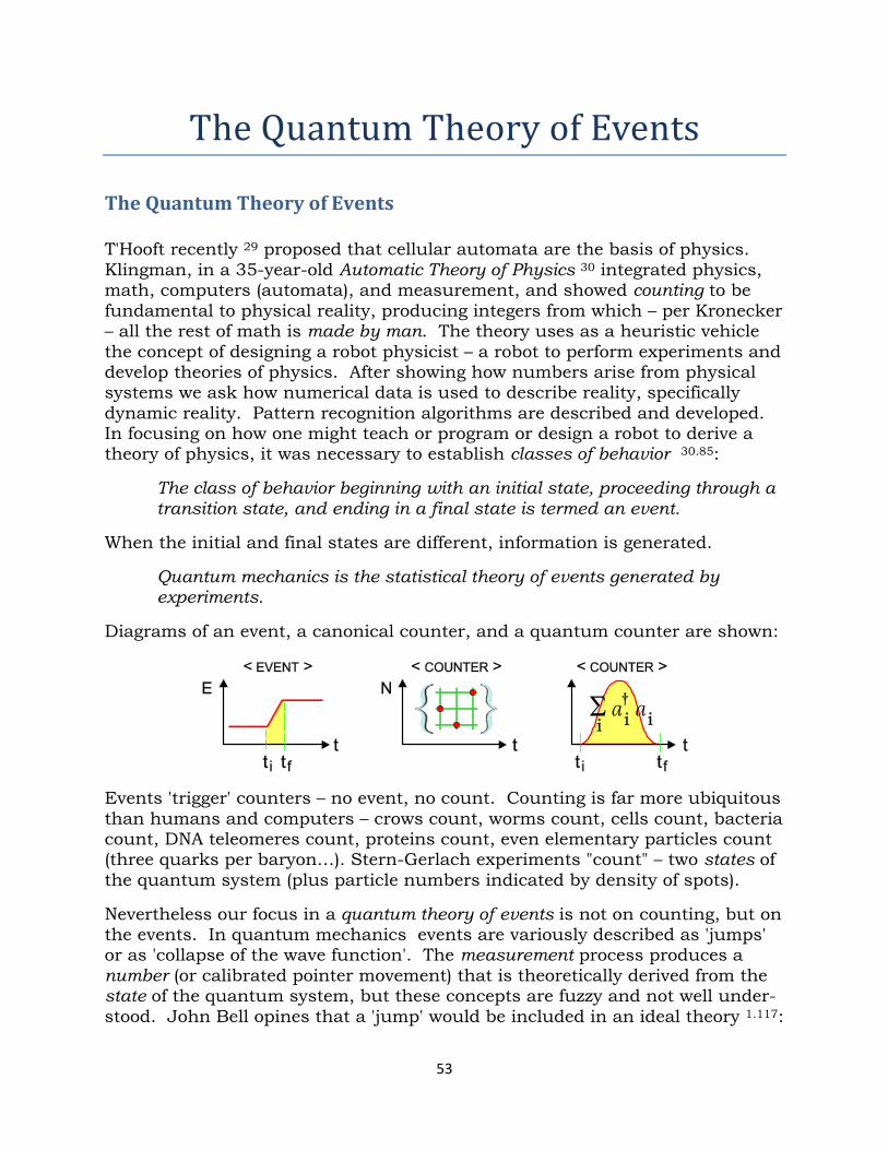
The Quantum Theory of Events

The Quantum Theory of Events T'Hooft recently 29 proposed that cellular automata are the basis of physics. Klingman, in a 35-year-old Automatic Theory of Physics 30 integrated physics, math, computers (automata), and measurement, and showed counting to be fundamental to physical reality, producing integers from which – per Kronecker – all the rest of math is made by man. The theory uses as a heuristic vehicle the concept of designing a robot physicist – a robot to perform experiments and develop theories of physics. After showing how numbers arise from physical systems we ask how numerical data is used to describe reality, specifically dynamic reality. Pattern recognition algorithms are described and developed. In focusing on how one might teach or program or design a robot to derive a theory of physics, it was necessary to establish classes of behavior 30.85:

The class of behavior beginning with an initial state, proceeding through a transition state, and ending in a final state is termed an event.

When the initial and final states are different, information is generated.

Quantum mechanics is the statistical theory of events generated by experiments.

Diagrams of an event, a canonical counter, and a quantum counter are shown:

Events 'trigger' counters – no event, no count. Counting is far more ubiquitous than humans and computers – crows count, worms count, cells count, bacteria count, DNA teleomeres count, proteins count, even elementary particles count (three quarks per baryon…). Stern-Gerlach experiments "count" – two states of the quantum system (plus particle numbers indicated by density of spots).

Nevertheless our focus in a quantum theory of events is not on counting, but on the events. In quantum mechanics events are variously described as 'jumps' or as 'collapse of the wave function'. The measurement process produces a number (or calibrated pointer movement) that is theoretically derived from the state of the quantum system, but these concepts are fuzzy and not well under-stood. John Bell opines that a 'jump' would be included in an ideal theory 1.117:

53

"… the fundamental theory [should] be about these more fundamental concepts… One line of development towards greater physical precision would be to have the [quantum] 'jumps' in the equation and not just in the talk – so it would come about as a dynamical process in dynamically defined conditions."

But jumps are not the only confusing aspect of quantum theory. Leifer 31 notes

"The status of the quantum state is one of the most controversial issues in the foundation of quantum theory. Is it a state of knowledge (an epistemic state), or a state of physical reality (an ontic state)?"

We will show that it is a restricted knowledge of a locally real physical property.

"An ontological model for […] experiments is an attempt to explain the quantum predictions in terms of some real physical properties – denoted and called ontic states – that exist independently of the experimenters…”

while a knowledge model leads to such questions as “What is precessing?” and to concepts such as collapse of the wavefunction. Recent theorems aiming to show that quantum states must be ontic have been proved in refinements of Bell’s hidden variable approach. And Leifer, based on the indistinguishability of non-orthogonal states, shows that epistemic explanations of indistinguish-ability become increasingly implausible as Hilbert space dimension grows. Hidden variables should allow prediction of measurement results; Leifer notes:

In general, the probability measure should be associated with the method of preparing ⟩ψ| rather than with ⟩ψ| itself.

Bell agrees 1.35 about the very essential role of apparatus:

“…the result of measurement does not actually tell us about some property previously possessed by the system, but about something which has come into being in the combination of system and apparatus."

In other words, something which has come into being during the transition from initial to final states. Of course, ontological models are required to reproduce quantum predictions, but for realistic models we must develop a theory of this transition behavior, which we do next. Alain Aspect1 ironically notes that "John Bell started his activity in physics at a time when the first quantum revolution had been so successful that nobody would 'waste time' in considering questions about the very basic concepts at work in quantum mechanics." Ironic because, 50 years later, few will 'waste time' considering questions about John Bell's ‘revolution’. Yet Aspect observes

"fundamental questions about the measurement problem … are not yet settled."

54

Energy Modes Coupled to a Common Variable We have seen that the energy of the precessing moment in an inhomogeneous field consists of two primary terms:

xdxBxBxE ⋅⋅∇+⋅−= ))(()()( µµ . 2- 1

If 0|| =dtd µ and θµµ cos|||| BB =⋅ this implies

xdgfxE

⋅+−= )()()( θθ 2- 2 where )(θf represents configurational energy, including the rotational kinetic energy of precession, and )(θg represents the force of the field gradient, which results in linear kinetic energy xdg

⋅)(θ . The two different energy modes depend on the variable θ . If local energy E is conserved the Energy-Exchange theorem applies.

The Energy-Exchange Theorem

Assume a physical system possesses two energy modes 0M and 1M with energy

0ε and 1ε — for example, a molecule’s vibrational and rotational modes. Assume both modes couple to a common physical variable, θ , and 0ε and 1ε are not separated by a quantum gap 0>∆ε . If the common variable θ varies with time the modes will exchange energy.

The total energy 10 εεε += where ⟩=⟩ ψεψ || iiH and total energy 10 HHH += is conserved:

000 1010 =+⇒=+⇒=dtd

ddH

dtd

ddH

dtdH

dtdH

dtdH θ

θθ

θ 010 =

+⇒

dtd

ddH

ddH θ

θθ

Since 0≠dtdθ

θθ ddH

ddH 10 −= 2- 3

and energy flows to mode 0M from mode 1M . QED

A simple example is the flow of energy from the gravitational energy mode to the kinetic energy of a particle in the Earth’s local gravitational field, where

Fzdd

⋅=0ε and zdmgd −=1ε . With shared variable θ the height, z , we have

Fzd

d=0ε and mg

zdd

−=1ε . 2- 4

55

From the Energy-Exchange theorem we expect:

010 =

+

tdzd

zdd

zdd εε

. 2- 5

Hence, if 0≠tdzd then 0)( =−+ mgF and therefore mgF = . As a second example, consider the Stern-Gerlach apparatus with energy modes

220 mv=ε and B

⋅−= µε1 where µ is the magnetic moment of the atom and B

is the inhomogeneous field the atom traverses, and which exerts a force25, 14.326

given by )( BF

⋅∇= µ . Translational kinetic energy of motion over distance xd is

xdBxdFd ⋅⋅∇=⋅= )(0 µε . 2- 6

Assume that the magnitude of the moment µ is constant and the precessional

angle between µ and B is θ and is common to both energies. According to the

Energy Exchange theorem, there is energy flow associated with the change in the common variable, θ , the initial angle of precession. But does the angle actually change? Bell says not, 1.141

"It might be supposed …that the magnetic field first pulls the little magnets into alignment with itself, like compass needles. [But this] is not dynamic-ally sound. The internal angular momentum, by gyroscopic action, should stabilize the angle between particle axis and magnetic field."

But Bell also says

"suppose the field points up, and that the strength of the field increases in the upward direction. Then a particle with south-north axis pointing up would be pulled up, one with axis pointing down would be pulled down."

Configurational energy θµµ cos00 BB −=⋅− is based on moment µ , and initial

field 0B

. Let BBB

∆+=+ 0 and consider the configurational energy after being

pulled up to field strength +B

. Assume configurational energy is conserved:

±± ⋅−=⋅− BB µµ 2- 7

But we assume that ±≡ µµ so

θµθµ ′∆±−=− cos)(cos 00 BBB

where the final angle θδθθ +=′ . Then (choosing the ‘+’ branch for B∆ ) we find

56

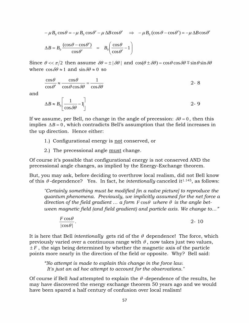
θµθµθµ ′∆−′−=− coscoscos 00 BBB θµθθµ ′∆−=′−−⇒ cos)cos(cos0 BB

−′

=′

′−=∆ 1

coscos

cos)cos(cos

00 θθ

θθθ BBB

Since 2πθ << then assume || δθδθ ±= and δθθδθθδθθ sinsincoscos)cos( =± where 1cos ≈δθ and 0sin ≈δθ so

δθδθθθ

θθ

cos1

coscoscos

coscos

=≈′

2- 8

and

−≈∆ 1

cos1

0 δθBB 2- 9

If we assume, per Bell, no change in the angle of precession: 0=δθ , then this implies 0=∆B , which contradicts Bell’s assumption that the field increases in the up direction. Hence either:

1.) Configurational energy is not conserved, or

2.) The precessional angle must change. Of course it’s possible that configurational energy is not conserved AND the precessional angle changes, as implied by the Energy-Exchange theorem. But, you may ask, before deciding to overthrow local realism, did not Bell know of this θ -dependence? Yes. In fact, he intentionally canceled it1.145, as follows:

"Certainly something must be modified [in a naïve picture] to reproduce the quantum phenomena. Previously, we implicitly assumed for the net force a direction of the field gradient … a form θcosF where θ is the angle bet-ween magnetic field (and field gradient) and particle axis. We change to…”

|cos|cosθθF . 2- 10

It is here that Bell intentionally gets rid of the θ dependence! The force, which previously varied over a continuous range with θ , now takes just two values,

F± , the sign being determined by whether the magnetic axis of the particle points more nearly in the direction of the field or opposite. Why? Bell said:

“No attempt is made to explain this change in the force law. It's just an ad hoc attempt to account for the observations."

Of course if Bell had attempted to explain the θ -dependence of the results, he may have discovered the energy exchange theorem 50 years ago and we would have been spared a half century of confusion over local realism!

57

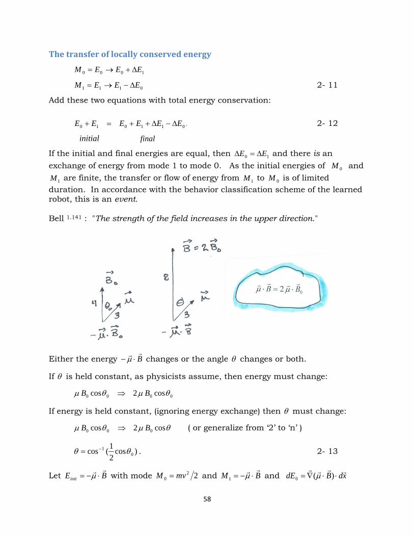
The transfer of locally conserved energy

1000 EEEM ∆+→=

0111 EEEM ∆−→= 2- 11

Add these two equations with total energy conservation:

011010 EEEEEE ∆−∆++=+ . 2- 12

initial final If the initial and final energies are equal, then 10 EE ∆=∆ and there is an exchange of energy from mode 1 to mode 0. As the initial energies of 0M and

1M are finite, the transfer or flow of energy from 1M to 0M is of limited duration. In accordance with the behavior classification scheme of the learned robot, this is an event.

Bell 1.141 : "The strength of the field increases in the upper direction."

Either the energy B

⋅− µ changes or the angle θ changes or both.

If θ is held constant, as physicists assume, then energy must change:

0000 cos2cos θµθµ BB ⇒ If energy is held constant, (ignoring energy exchange) then θ must change:

θµθµ cos2cos 000 BB ⇒ ( or generalize from ‘2’ to ‘n’ )

)cos21(cos 0

1 θθ −= . 2- 13

Let BEinit

⋅−= µ with mode 22

0 vmM = and BM

⋅−= µ1 and xdBdE ⋅⋅∇= )(0 µ

58

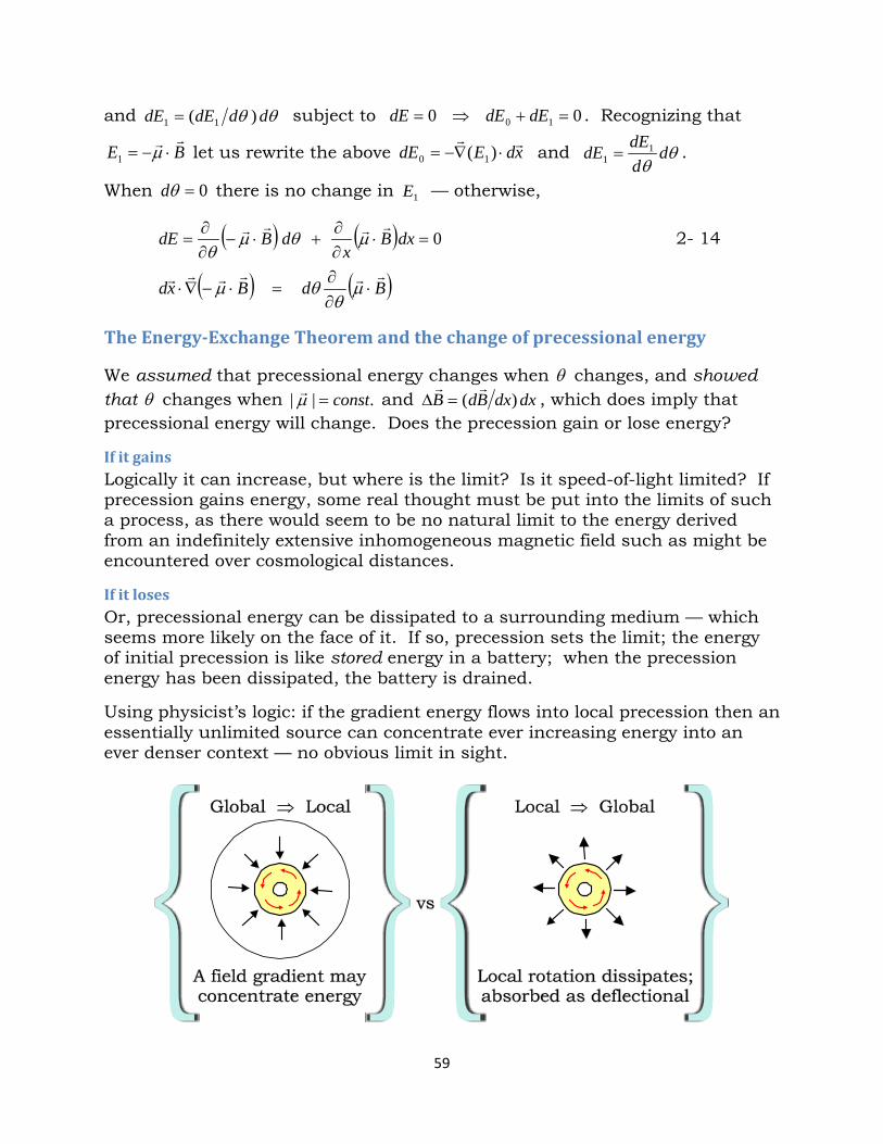
and θθ dddEdE )( 11 = subject to 00 10 =+⇒= dEdEdE . Recognizing that

BE

⋅−= µ1 let us rewrite the above xdEdE ⋅∇−= )( 10 and θ

θd

ddEdE 1

1 = .

When 0=θd there is no change in 1E — otherwise,

( ) ( ) 0=⋅∂∂

+⋅−∂∂

= dxBx

dBdE µθµ

θ 2- 14

( ) ( )BdBxd

⋅

∂∂

=⋅−∇⋅ µθ

θµ

The Energy-Exchange Theorem and the change of precessional energy

We assumed that precessional energy changes when θ changes, and showed that θ changes when .|| const=µ and dxdxBdB )(

=∆ , which does imply that

precessional energy will change. Does the precession gain or lose energy?

If it gains Logically it can increase, but where is the limit? Is it speed-of-light limited? If precession gains energy, some real thought must be put into the limits of such a process, as there would seem to be no natural limit to the energy derived from an indefinitely extensive inhomogeneous magnetic field such as might be encountered over cosmological distances.

If it loses Or, precessional energy can be dissipated to a surrounding medium — which seems more likely on the face of it. If so, precession sets the limit; the energy of initial precession is like stored energy in a battery; when the precession energy has been dissipated, the battery is drained. Using physicist’s logic: if the gradient energy flows into local precession then an essentially unlimited source can concentrate ever increasing energy into an ever denser context — no obvious limit in sight.

59

Where does it go? But if the precessional energy dissipates, where does the exchanged energy go, and how? There are two cases: a) it is exchanged locally through tight coupling, or b) it is distributed globally through looser coupling. The first case, coupling the precession energy to the local deflection energy is compatible with our energy exchange theorem. The second case could entail radiation of dipole electromagnetic energy via coupling to the field, and distribute this to the ends of the universe. It seems likely that precession dissipates energy to the local environment by deflecting the particle ( and agrees with Stern-Gerlach data ). Energy accumulates locally only if the binding energy becomes negative, as in electrons bound to nuclei, or quarks bound together. Else, either design (focused lasers, microwave ovens…) or gravitic self-interaction is involved.

So without solving any equations we can convince ourselves that the energy of precession will be dissipated and will be absorbed by deflectional energy – thus deflection energy 0ε is absorber, and precession energy 1ε is a finite source, and the energy exchange theorem implies

θε

θε

dd

dd 10 −= 2- 15

and, integrated over θd we find −=0εd 0εd . Here we have considered no physical issues other than scale — the unlimited global sink or source versus the limited local source or sink. Logic indicates that local flow is outward (entropic) – flow terminates when the local source is exhausted. The alternative is a never-ending conversion of local energy extract-ed everywhere globally and concentrated locally, antientropic and limit seeking! In the above we have recognized that the detailed dynamics of three interacting vector entities )),(,( vxB µ are in general too complex to calculate. In this regard Grover 67 recently pointed out that:

"… there are only a few interacting quantum systems that can be solved exactly…"

But such classical tools as Poisson Brackets, applied to conservation of energy,

0=dtdH , have allowed us to show that different energy modes coupled to a common variable will exchange energy regardless of the complex dynamics! So we are encouraged to continue analyzing other physical aspects of change of precessional energy, although, heretofore, in quantum mechanics,

… such change has merely been assumed not to occur, and this assumption treated as a fundamental basis of quantum mechanics.

60

Quantum Precession

It is customary — as seen in Susskind’s videos and in Bell’s claim that the internal angular momentum should stabilize the angle between the particle axis and the field — to treat the particle as if it continues to precess, with the components perpendicular to the field being averaged to zero. So the quantum mechanical result is semi-compatible with the classical treatment, in which the off-axis components also average to zero. The quantum mechanical average is interpreted as ‘what is expected’ for a magnetic moment precessing in the field. But it is precession that enables the spin-component illusion – the belief that the Stern-Gerlach experiment measures any spin component of three spin components, which we will call λλλλ =),,( zyx . If we measure the z-axis component — assumed aligned with the 1D-field — we find 1± , indicating alignment or anti-alignment – the only two possible choices for the z-axis. But if we compute the quantum expectation values of the off-z-axis components, they average to zero, just as the classical analog would predict. As the z-axis "component" is constant, its time derivative is zero, and therefore the component does not vary. As this component is perceived as the projection onto the z-axis of a precessing dipole moment, the illusion is maintained, perceived as backed up by experimental proof. It may not have occurred to Bell that zero averages of all off-axis components, consistent with the precessing model, are also 100% consistent with the energy exchange model wherein the entire moment becomes aligned and there are no off-axis components. In other words an energy-exchange-theorem-based theory is absolutely consistent with the data — but not with the reigning paradigm.

“Zero average component” is also compatible with “no precession”. Thus, the factual quantum mechanical results are actually compatible with our energy-exchange interpretation of the physics, in which the moment aligns with the field and does not precess! So we will consider real 3D spins as measured using a 1D Stern-Gerlach apparatus to align with the field.

The quantum assumption is that, because components of angular momentum do not commute, they are not simultaneously measurable, and thus measure-ments are interpreted as one spin component of quantized angular momentum. The concept of precession—whatever is precessing —is key to the interpretation and to support of the ‘only-one-component-can-be-measured’ story. Of course, missing in the standard interpretation is conversion of rotational energy LB

⋅ to

kinetic energy 22mv and re-alignment of the spin. We will revisit this aspect of the problem when we discuss counterfactual reasoning, but first we ask how the energy exchange interpretation can be best incorporated into the current formalism of quantum physics.

61

Quantum Transformation theory

Since Bell’s naive analysis produces a local realism model that does not jive with results of experiment, many physicists have concluded that local realism models are incompatible with quantum correlations — a very high price to pay. But only local realism models in which spin is unperturbed will fail to match experimental results. Bell says1.117

"The concept of 'measurement' becomes so fuzzy on reflection that it is quite surprising to have it appearing in physical theory at the most fundamental level … [D]oes not any analysis of measurement require concepts more fundamental than measurement?"

Bell was, perhaps unwittingly, noting that quantum fishermen are not so much measuring physical reality in sea-space, as transforming sea-space by removing and recording fish greater than 3 inches in size. For them, ‘hidden parameters’ below 3 inches remain hidden. Similarly, Stern-Gerlach transforms the atomic distribution by removing all partially aligned dipoles and replacing them with fully aligned dipoles and recording these.

The spin λ undergoes a transformation!

Once λ has been transformed to a+ , all following tests will produce a+ . But if a is changed (say z to x ) then a new transformation occurs; the measurement value becomes 1+ or 1− again (with average value zero). Although this seems obvious, physicists, based on the "quantum theory of measurement" (3” nets) have tied themselves in knots and, en mass, decided to give up local realism.

Santos states32 quantum mechanics consists of two quite different ingredients: "…the formalism (…) and the theory of measurement, both of which are postulated independently. Actually the two ingredients are to some extent contradictory, because quantum evolution is continuous and deterministic except during the measurement, where the "collapse of the wave function" is discontinuous and stochastic."

In the spirit of Santos we ask how we can accommodate the formalism and the theory of measurement. Perhaps they are separable, such that the experiment can be represented by a Q-operator which represents the physics evolution of the physical state λ and the measurement by the experimental setting a : ),( aQ λ

Gordon Watson, taking Bell seriously, concluded that analysis of measurement does require new concepts. Specifically, Watson 33

“takes transformation to be a concept more fundamental than measurement.'"

62

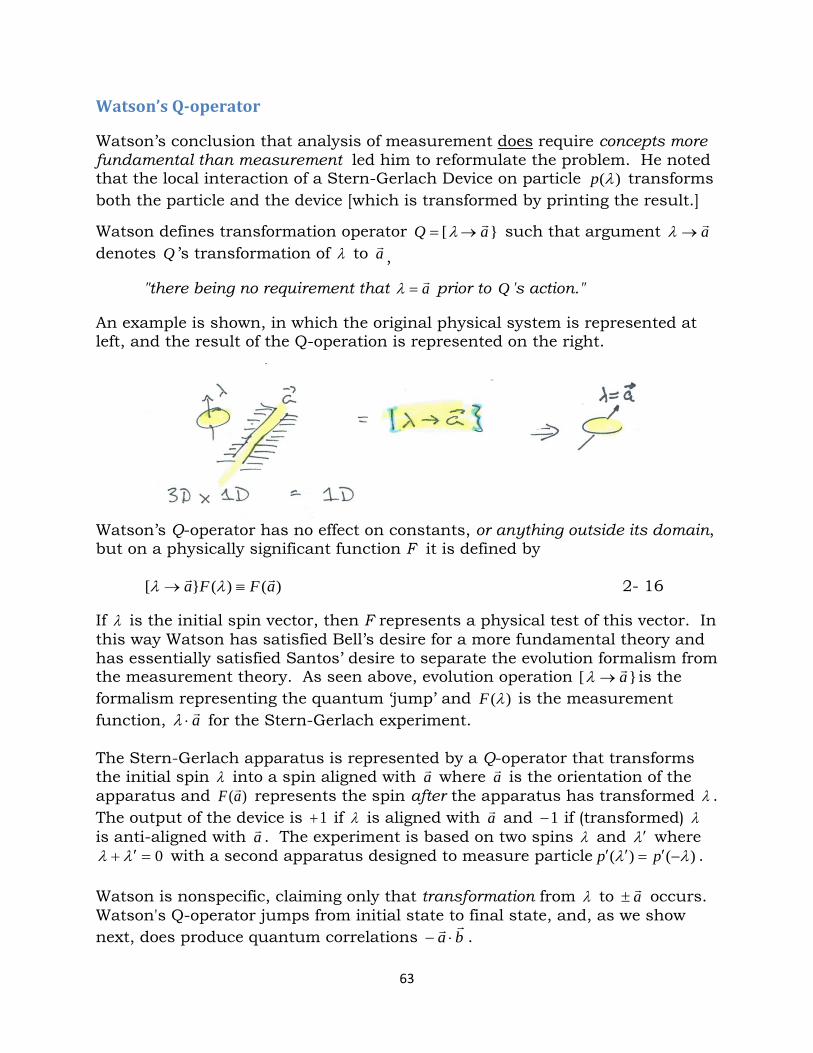
Watson’s Q-operator Watson’s conclusion that analysis of measurement does require concepts more fundamental than measurement led him to reformulate the problem. He noted that the local interaction of a Stern-Gerlach Device on particle )(λp transforms both the particle and the device [which is transformed by printing the result.] Watson defines transformation operator [ aQ

→= λ such that argument a→λ denotes Q ’s transformation of λ to a ,

"there being no requirement that a=λ prior to Q 's action."

An example is shown, in which the original physical system is represented at left, and the result of the Q-operation is represented on the right.

Watson’s Q-operator has no effect on constants, or anything outside its domain, but on a physically significant function F it is defined by

)()([ aFFa ≡→ λλ 2- 16

If λ is the initial spin vector, then F represents a physical test of this vector. In this way Watson has satisfied Bell’s desire for a more fundamental theory and has essentially satisfied Santos’ desire to separate the evolution formalism from the measurement theory. As seen above, evolution operation [ a→λ is the formalism representing the quantum ‘jump’ and )(λF is the measurement function, a⋅λ for the Stern-Gerlach experiment. The Stern-Gerlach apparatus is represented by a Q-operator that transforms the initial spin λ into a spin aligned with a where a is the orientation of the apparatus and )(aF represents the spin after the apparatus has transformed λ . The output of the device is 1+ if λ is aligned with a and 1− if (transformed) λ is anti-aligned with a . The experiment is based on two spins λ and λ′ where

0=′+ λλ with a second apparatus designed to measure particle )()( λλ −′=′′ pp . Watson is nonspecific, claiming only that transformation from λ to a± occurs. Watson's Q-operator jumps from initial state to final state, and, as we show next, does produce quantum correlations ba

⋅− .

63

Watson’s refutation of Bell’s Theorem A Stern-Gerlach apparatus represented by a Q -operator transforms the initial spin λ into a spin aligned with a and )(aF measures the spin after transform-ation. In reality we do not know until measurement occurs whether the result is 1± , therefore the application of the Q-operator has the form [ a±→λ . The EPRB experiment is based on two spins λ and λ′ with 0=′+ λλ and a second apparatus designed to measure particle )()( λλ −′=′′ pp is represented by Q operating on G. To proceed we recall that Bell’s theorem is formulated as:

If ∫ =−=±==±== ±± ;1)();,(1),(;1),( λρλλλλ dbABbBAaA

Then ∫∫ ⋅−≠−=≡⟩⟨ babAaAdbBaAdAB ),(),()(),(),()( λλλρλλλλρλ 2- 17

where A and B represent measurements of spin; λ is the hidden variable that is assumed to deterministically cause the measurement results. To reformulate this in terms of more fundamental operations, Watson replaces Bell’s ),( λaA by the term )([),( λλλ FaaQ

±→= and ),( λbB

by )([),( λλλ ′±→′=′ GbbQ

, respect-ing the locality of the terms via the use of primed spin. Watson thus translates the terms in Bell’s integral as follows:

=),(),( λλ bBaA )([)([ λλλλ ′±→′±→ GbFa

. 2- 18

We will later analyze the error in Bell's approach, but for the moment we focus on interpreting Watson’s more fundamental approach. Reading Bell's analysis is almost meaningless for one who does not understand quantum mechanical formalism, and we assume at this point that the reader is not yet familiar with Watson’s formalism. Specifically, Bell uses λ as if it were equally applicable to A and B, while Watson respects the fact that A and B are located remotely from each other and if Alice measures spin λ , then Bob measures spin λ′ , despite the fact that the two are highly correlated. Thus Q is a local operation, while this fact is glossed over by Bell's use of λ with both A and B. To illustrate Watson’s approach and to help familiarize the reader with the local realism built into Watson’s approach, we show a formal picture of an entire EPRB experiment below, worthy of study before proceeding. Key to interpreting the Q-operator is to pay attention to the domain of the operator. A Q-operation is truly a local operation, operating only on elements in its local domain. Thus the operator [ a→λ has no effect on λ′ or on [ b

→′λ and vice versa.

The power of Watson’s concise formalism is shown by the following summary:

±± =±=⋅′±→′→′′→=′+←←←±⋅=±= BbbppaaA )1()([)(0)(])()1( λλλλλλλλ .

64

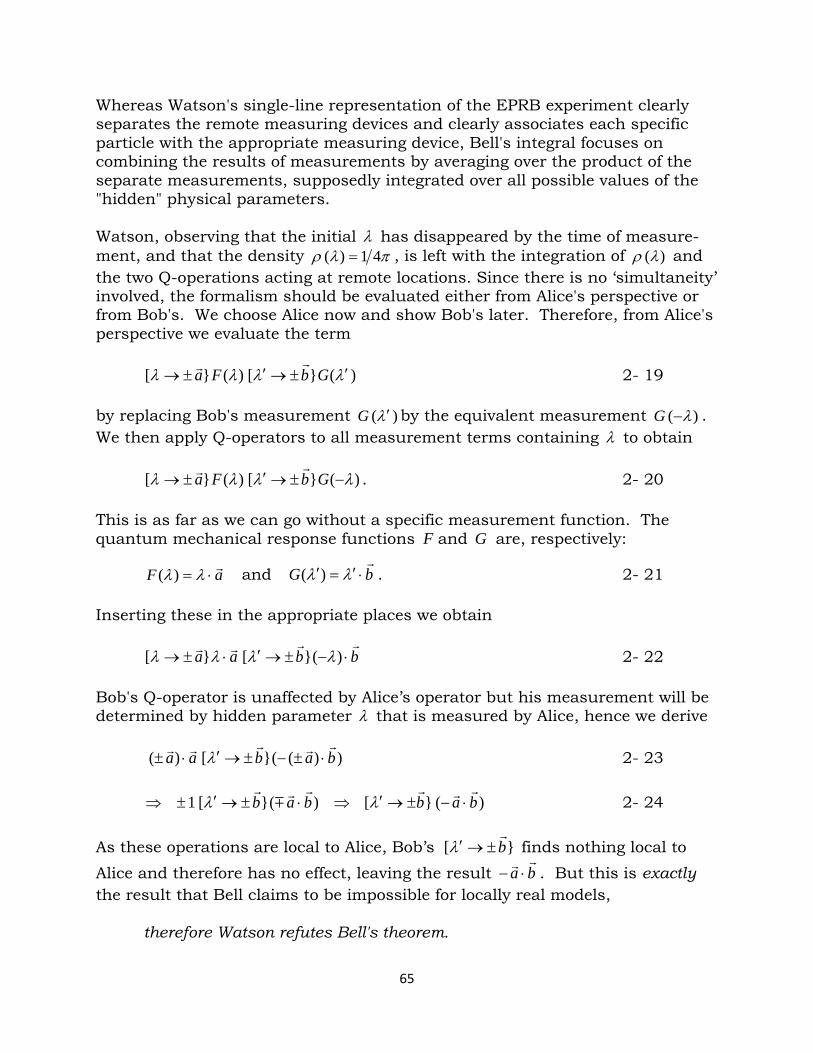
Whereas Watson's single-line representation of the EPRB experiment clearly separates the remote measuring devices and clearly associates each specific particle with the appropriate measuring device, Bell's integral focuses on combining the results of measurements by averaging over the product of the separate measurements, supposedly integrated over all possible values of the "hidden" physical parameters. Watson, observing that the initial λ has disappeared by the time of measure-ment, and that the density πλρ 41)( = , is left with the integration of )(λρ and the two Q-operations acting at remote locations. Since there is no ‘simultaneity’ involved, the formalism should be evaluated either from Alice's perspective or from Bob's. We choose Alice now and show Bob's later. Therefore, from Alice's perspective we evaluate the term )([)([ λλλλ ′±→′±→ GbFa

2- 19

by replacing Bob's measurement )(λ′G by the equivalent measurement )( λ−G . We then apply Q-operators to all measurement terms containing λ to obtain )([)([ λλλλ −±→′±→ GbFa

. 2- 20

This is as far as we can go without a specific measurement function. The quantum mechanical response functions F and G are, respectively:

aF ⋅= λλ)( and bG

⋅′=′ λλ )( . 2- 21

Inserting these in the appropriate places we obtain

bbaa⋅−±→′⋅±→ )([[ λλλλ 2- 22

Bob's Q-operator is unaffected by Alice’s operator but his measurement will be determined by hidden parameter λ that is measured by Alice, hence we derive

))(([)( babaa⋅±−±→′⋅± λ 2- 23

)([)([1 babbab

⋅−±→′⇒⋅±→′±⇒ λλ 2- 24

As these operations are local to Alice, Bob’s [ b

±→′λ finds nothing local to

Alice and therefore has no effect, leaving the result ba⋅− . But this is exactly

the result that Bell claims to be impossible for locally real models,

therefore Watson refutes Bell's theorem.

65

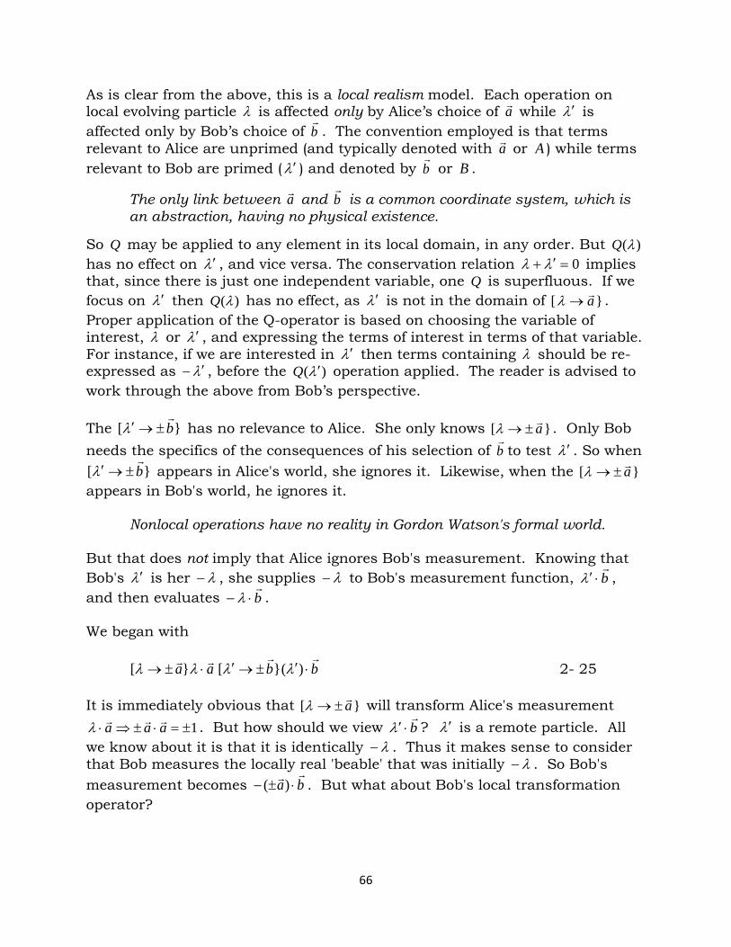
As is clear from the above, this is a local realism model. Each operation on local evolving particle λ is affected only by Alice’s choice of a while λ′ is affected only by Bob’s choice of b

. The convention employed is that terms

relevant to Alice are unprimed (and typically denoted with a or A ) while terms relevant to Bob are primed (λ′ ) and denoted by b

or B .

The only link between a and b

is a common coordinate system, which is an abstraction, having no physical existence.

So Q may be applied to any element in its local domain, in any order. But )(λQ has no effect on λ′ , and vice versa. The conservation relation 0=′+ λλ implies that, since there is just one independent variable, one Q is superfluous. If we focus on λ′ then )(λQ has no effect, as λ′ is not in the domain of [ a→λ . Proper application of the Q-operator is based on choosing the variable of interest, λ or λ′ , and expressing the terms of interest in terms of that variable. For instance, if we are interested in λ′ then terms containing λ should be re-expressed as λ′− , before the )(λ′Q operation applied. The reader is advised to work through the above from Bob’s perspective. The [ b

±→′λ has no relevance to Alice. She only knows [ a±→λ . Only Bob

needs the specifics of the consequences of his selection of bto test λ′ . So when

[ b

±→′λ appears in Alice's world, she ignores it. Likewise, when the [ a±→λappears in Bob's world, he ignores it.

Nonlocal operations have no reality in Gordon Watson's formal world. But that does not imply that Alice ignores Bob's measurement. Knowing that Bob's λ′ is her λ− , she supplies λ− to Bob's measurement function, b

⋅′λ ,

and then evaluates b⋅− λ .

We began with bbaa

⋅′±→′⋅±→ )([[ λλλλ 2- 25

It is immediately obvious that [ a±→λ will transform Alice's measurement

1±=⋅±⇒⋅ aaa λ . But how should we view b⋅′λ ? λ′ is a remote particle. All

we know about it is that it is identically λ− . Thus it makes sense to consider that Bob measures the locally real 'beable' that was initially λ− . So Bob's measurement becomes ba

⋅±− )( . But what about Bob's local transformation

operator?

66

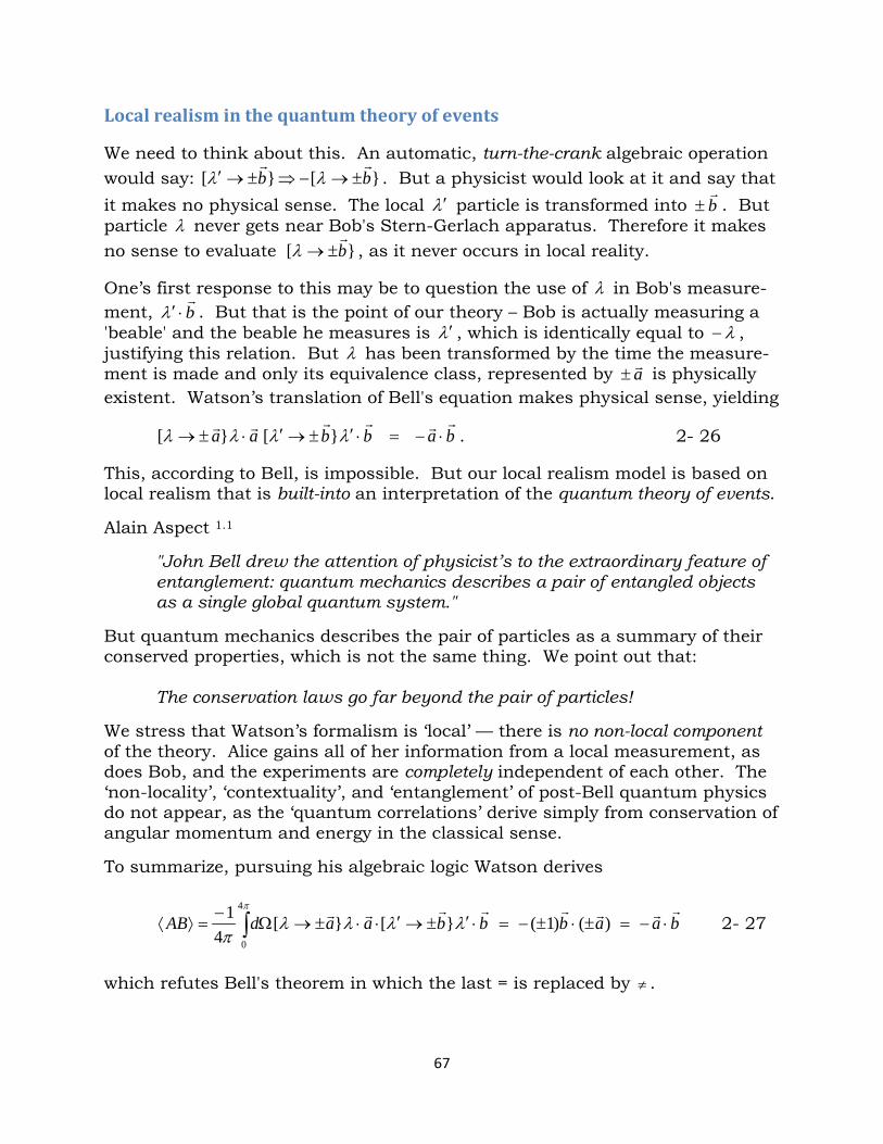
Local realism in the quantum theory of events We need to think about this. An automatic, turn-the-crank algebraic operation would say: [[ bb

±→−⇒±→′ λλ . But a physicist would look at it and say that

it makes no physical sense. The local λ′ particle is transformed into b

± . But particle λ never gets near Bob's Stern-Gerlach apparatus. Therefore it makes no sense to evaluate [ b

±→λ , as it never occurs in local reality.

One’s first response to this may be to question the use of λ in Bob's measure-ment, b

⋅′λ . But that is the point of our theory – Bob is actually measuring a

'beable' and the beable he measures is λ′ , which is identically equal to λ− , justifying this relation. But λ has been transformed by the time the measure-ment is made and only its equivalence class, represented by a± is physically existent. Watson’s translation of Bell's equation makes physical sense, yielding

babbaa⋅−=⋅′±→′⋅±→ λλλλ [[ . 2- 26

This, according to Bell, is impossible. But our local realism model is based on local realism that is built-into an interpretation of the quantum theory of events.

Alain Aspect 1.1

"John Bell drew the attention of physicist’s to the extraordinary feature of entanglement: quantum mechanics describes a pair of entangled objects as a single global quantum system."

But quantum mechanics describes the pair of particles as a summary of their conserved properties, which is not the same thing. We point out that:

The conservation laws go far beyond the pair of particles! We stress that Watson’s formalism is ‘local’ — there is no non-local component of the theory. Alice gains all of her information from a local measurement, as does Bob, and the experiments are completely independent of each other. The ‘non-locality’, ‘contextuality’, and ‘entanglement’ of post-Bell quantum physics do not appear, as the ‘quantum correlations’ derive simply from conservation of angular momentum and energy in the classical sense. To summarize, pursuing his algebraic logic Watson derives

baabbbaadAB⋅−=±⋅±−=⋅′±→′⋅⋅±→Ω

−=⟩⟨ ∫ )()1([[

41 4

0

λλλλπ

π

2- 27

which refutes Bell's theorem in which the last = is replaced by ≠ .

67

The Perspective of Local Realism For most quantum physicists this is quite a shift in perspective. For 50 years Bell has employed counterfactual reasoning to deny the possibility of local realistic models of physical reality, concluding that both particles are non-locally "entangled", all based on Bell’s ∫ ⋅−≠ bad

λ and his 'merging' of the two

particles into one λ , spanning the entire space superluminally. For example, papers on quantum states and reality are adamant 34:

"Unfortunately, as shown later by Bell, Einstein's specific argument for incompleteness was based on the false premise (locality). [and] separated subsystems would involve superluminal influences of measurement choices upon ontic variables."

But Alain Aspect, who first confirmed that Bell's inequality is violated by Nature, claims that such nonlocal entanglement is "difficult to swallow." So now, despite physical reasoning based on the energy exchange theorem, the typical quantum mechaniker (whose quantum knowledge after all extends far beyond Stern-Gerlach) probably has the feeling that Watson has figured out a 'trick' that yields the desired result but need not be taken seriously. Therefore we need to show that Watson’s formalism provides 'local beables' and produces the required probability, thus not only fulfilling Einstein's desire for local realism but also his belief that a complete theory was possible, subject to1.91:

"The formal relations [of quantum mechanics] – i.e., it's entire mathematical formalism – will probably have to be contained, in the form of logical inferences, in every useful future theory."

Watson’s formalism is exactly what Bell speculated about 1.41 :

"… a future theory will not be intrinsically ambiguous and approximate. Such a theory could not be fundamentally about 'measurement'… not about 'observables' but about 'beables'."

Watson’s ‘dynamic equivalence classes’ are equivalent to Bell’s beables and are similar to Nobelist G. ‘t Hooft’s mapping of events into equivalence classes29.186

“Each info-equivalence class corresponds to an element of the ontological basis of a quantum theory. [and] classical states are obviously represented by the equivalence classes.”

68

Dynamic Equivalence Classes Watson’s Q -operator, via result +A , reveals a dynamic equivalence class +a .

“The dynamic equivalence class +a reveals a previously-hidden pre-existing real property of the [ pretested ] particle.”

Thus for any a the Q -operator establishes a dynamic equivalence class. Watson defines an equivalence relation ~ on the set 3R⊂Λ of the spin-related parameter λ as: has the same output under Q . That is, under the equivalence relation ~ on Λ , two spin parameters are equivalent if the Q -operator maps them to the same output. Under the mapping [ a±→λ , Λ is spanned by two dynamic equivalence classes, defined on the sets

~| 33 RaRa ∈+⊂Λ∈≡+ λλ and ~| 33 RaRa ∈−⊂Λ∈≡− λλ Thus 3: RVQ ⊂→Λ assigns every object Λ∈λ to exactly one element VQ ∈)(λ where V is the space of three vectors. Specifically, the measurement result

1+=≡+ AA reveals the previously-hidden pre-existing dynamic equivalence class +a to which λ belongs. The correlation between operations and equivalence classes:

[ a±→λ the operation transforming λ based on Alice's setting a

)( ±∈ aλ λ belongs to dynamic equivalence class −+ ⊗ aa The equivalence class defines a hidden pre-existing property, which refutes Bell's theorem in all its manifestations, demonstrating a local parameter which leads to correlations, ba

⋅− . Watson invokes no physical arguments, only

mathematical logic. His theory applies to any realistic physical interpretation that is compatible with the experimental results. His "dynamic equivalence class" may be a broader category than has typically been sought, but it never-theless satisfies all of Bell's requirements. Recall, Bell clearly stated that1.117

"… the fundamental theory [should] be about these more fundamental concepts… One line of development towards greater physical precision would be to have the [quantum] 'jumps' [or mergings] in the equation and not just in the talk – so it would come about as a dynamical process in dynamically defined conditions."

69

Q-operator and Probability The ‘jump’ that Bell desires is built-into Watson’s Q-operator, symbolized by the arrow → . The fact that the Stern-Gerlach apparatus maps any member of the equivalence class into output +A or −A implies that it is impossible to recapture the original λ input to the device. Information is irrevocably lost. The Q operator reveals the dynamic equivalence class of not only the local particle but its far-off "twin", thus allowing instant prediction of the remote 'measurement' without in any way implying either non-locality or action-at-a-distance. But is this just a ‘trick’? How does this relate to quantum mechanics? In an FQXi article, “Why Quantum?” 35 Colin Stuart notes:

"…any theory worthy of replacing quantum mechanics would still need to assign probabilities to the outcomes of experiments…"

If relation )|( ZXP denotes normalized prevalence (or probability) of X given Z, dynamic equivalence classes are akin to Bayesian updating in the expression

)|()|()|()|()|( YZXPZYPXZYPZXPZXYP == 2- 28

when X and Y are causally independent, in the sense that neither exerts any direct causal influence on the other. If quantum states are viewed as epistemic (informative) rather than ontic (real) then the "collapse of the wave function" is viewed as "Bayesian updating" of information/knowledge, as opposed to the more mysterious interpretation of a real ‘superposition of states’ collapsing. Watson then notes that since

⟩⟨=⋅−=±⋅±−=⋅±→⋅±→−= ABbaabbbaaAB )()1([[ λλλλ 2- 29

he establishes the consequential distribution of 1± as a function of a and b.

Having already derived the relation baAB⋅−=⟩⟨ (contradicting Bell) we simply

recall that ⟩⟨AB is the expectation value of the product of A with B . But, by definition, if a random variable X can take value 1x with probability )( 11 xPP = , value 2x with probability 2P , and so on, then the expectation value of the random variable X is defined as

∑=+++=⟩⟨j

jjkk xPxPxPxPxX )(2211 2- 30

where

1=∑j

jP . 2- 31

70

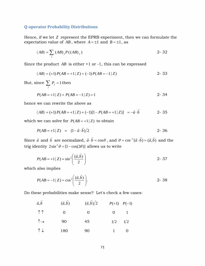
Q-operator Probability Distributions Hence, if we let Z represent the EPRB experiment, then we can formulate the expectation value of AB , where 1±=A and 1±=B , as

))(()( jj

j ABPABAB ∑=⟩⟨ 2- 32

Since the product AB is either +1 or -1, this can be expressed

)|1()1()|1()1( ZABPZABPAB −=−++=+=⟩⟨ 2- 33

But, since 1=∑j

jP then

1)|1()|1( =−=++= ZABPZABP 2- 34

hence we can rewrite the above as

baZABPZABPAB⋅−=+=−−++=+=⟩⟨ )]|1(1[)1()|1()1( 2- 35

which we can solve for )|1( ZABP += to obtain

2)1()|1( baZABP⋅−=+= 2- 36

Since a and b are normalized, θcos=⋅ba

, and ),()(cos 1 baba

=⋅= −θ and the

trig identity )]2cos(1[sin2 2 θθ −= allows us to write

=+=

2),(sin)|1( 2 baZABP

2- 37

which also implies

=−=

2),(cos)|1( 2 baZABP

. 2- 38

Do these probabilities make sense? Let's check a few cases: ba

, ),( ba

2),( ba

)1(+P )1(−P

↑↑ 0 0 0 1

↑→ 90 45 21 21

↓↑ 180 90 1 0

71

This distribution agrees with Bell, who says1.153: “According to quantum mechanics, however, for example with some practical approximation to the EPRB gedanken set up, we can have approximately 1.146, 3.88 :

bababababaE⋅−=−−=

−

−

−

= )cos(2

cos2

sin),( 22 2- 39

The probability for random variable A to yield +=+ A1 is 21 while the probability for −A is 21 also.

1)()( =+ −+ APAP independent of a (and b) 2- 40

and similarly

21)()( == −+ BPBP independent of b (and a ) 2- 41

But we found above that ),()( bafABP

= , therefore

)|()|()|( ZBPZAPZBAP ++++ ≠ 2- 42 which differs from Bell’s equation (9) and hence (10) 1.243, which Bell interprets as A and B having no dependence on one another, nor on the settings of the remote polarizers (b

and a ) respectively.

Watson thus refutes Bell’s conclusion that causal independence should equate to statistical independence, quoting 58 Arthur Fine:

“One general issue raised by the debates over locality is to understand the connection between stochastic independence (probabilities multiply) and genuine physical independent (no mutual influence). It is the latter that is at issue in ‘locality’, but it is the former that goes proxy for it in the Bell-like calculations. We need to press harder and deeper in our analysis here,”

Watson says of the above:

“Thus, given such physical correlations as those in EPRB, statistical independence does not equate to causal independence under local causality.

He mentions an analogy with pear and apple crops, which grow in the same climate. Neither causes the other to grow, but local physical reality establishes a physical correlation between these crops. Just as, with Q, we have physical correlations and consequent dynamic equivalence classes in our math/logic. So Watson’s equivalence classes are akin to Bayesian updating when a and b

are causally independent, neither exerting direct causal influence on the other.

72

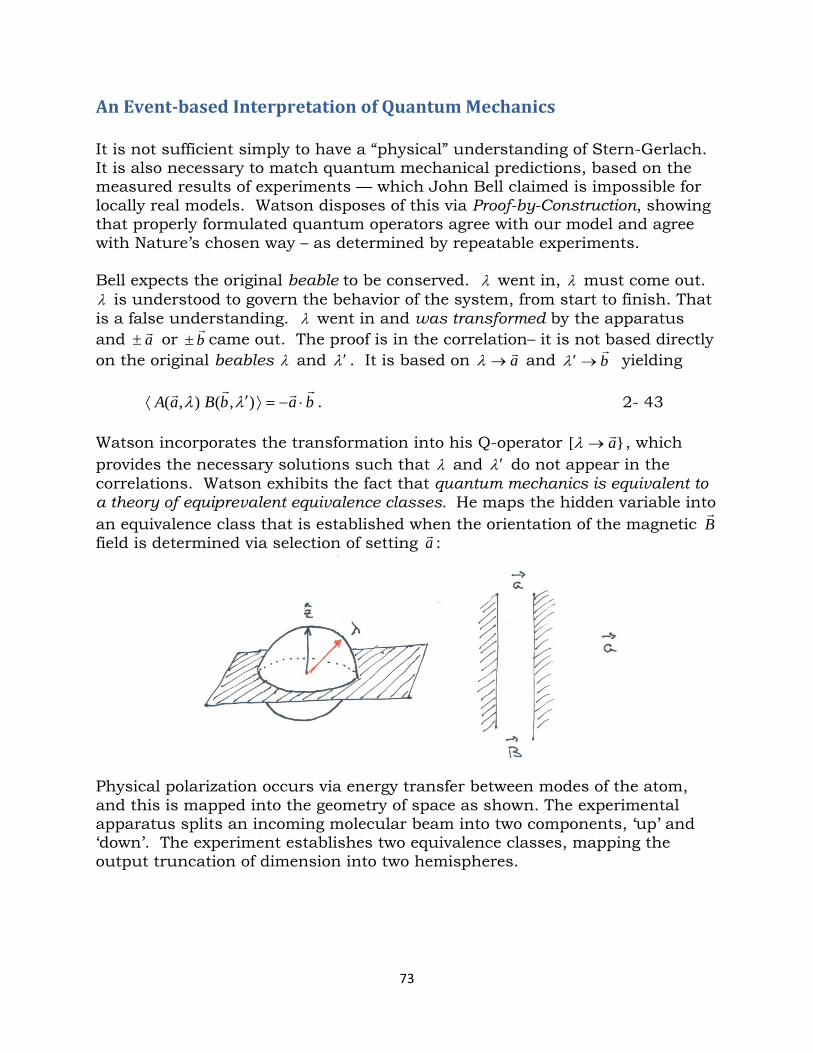
An Event-based Interpretation of Quantum Mechanics It is not sufficient simply to have a “physical” understanding of Stern-Gerlach. It is also necessary to match quantum mechanical predictions, based on the measured results of experiments — which John Bell claimed is impossible for locally real models. Watson disposes of this via Proof-by-Construction, showing that properly formulated quantum operators agree with our model and agree with Nature’s chosen way – as determined by repeatable experiments. Bell expects the original beable to be conserved. λ went in, λ must come out. λ is understood to govern the behavior of the system, from start to finish. That is a false understanding. λ went in and was transformed by the apparatus and a± or b

± came out. The proof is in the correlation– it is not based directly

on the original beables λ and λ′ . It is based on a→λ and b

→′λ yielding

babBaA⋅−=⟩′⟨ ),(),( λλ . 2- 43

Watson incorporates the transformation into his Q-operator [ a→λ , which provides the necessary solutions such that λ and λ′ do not appear in the correlations. Watson exhibits the fact that quantum mechanics is equivalent to a theory of equiprevalent equivalence classes. He maps the hidden variable into an equivalence class that is established when the orientation of the magnetic B

field is determined via selection of setting a :

Physical polarization occurs via energy transfer between modes of the atom, and this is mapped into the geometry of space as shown. The experimental apparatus splits an incoming molecular beam into two components, ‘up’ and ‘down’. The experiment establishes two equivalence classes, mapping the output truncation of dimension into two hemispheres.

73

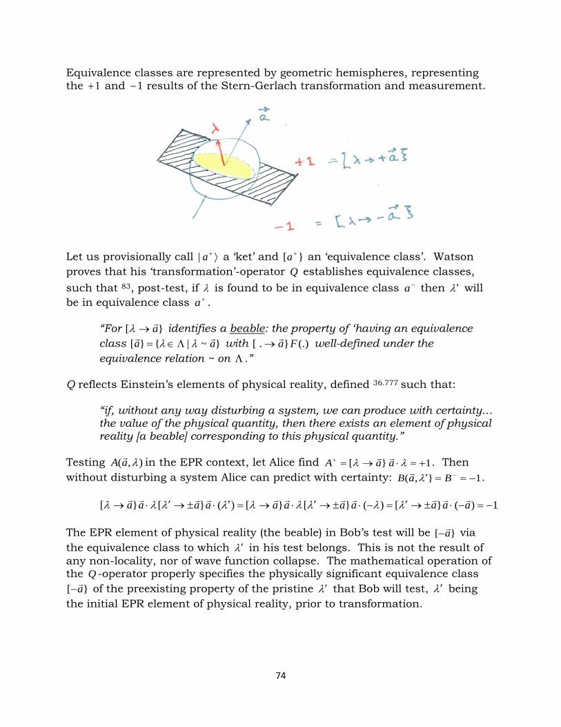
Equivalence classes are represented by geometric hemispheres, representing the 1+ and 1− results of the Stern-Gerlach transformation and measurement.

Let us provisionally call ⟩+a| a ‘ket’ and [ +a an ‘equivalence class’. Watson proves that his ‘transformation’-operator Q establishes equivalence classes, such that 83, post-test, if λ is found to be in equivalence class −a then λ′ will be in equivalence class +a .

“For [ a→λ identifies a beable: the property of ‘having an equivalence class ~|[ aa λλ Λ∈= with (.).[ Fa→ well-defined under the equivalence relation ~ on Λ .”

Q reflects Einstein’s elements of physical reality, defined 36.777 such that:

“if, without any way disturbing a system, we can produce with certainty… the value of the physical quantity, then there exists an element of physical reality [a beable] corresponding to this physical quantity.”

Testing ),( λaA in the EPR context, let Alice find 1[ +=⋅→=+ λλ aaA . Then without disturbing a system Alice can predict with certainty: 1,( −==′ −BaB λ .

1)([)([[)([[ −=−⋅±→′=−⋅±→′⋅→=′⋅±→′⋅→ aaaaaaaaaaa λλλλλλλλλ

The EPR element of physical reality (the beable) in Bob’s test will be [ a− via the equivalence class to which λ′ in his test belongs. This is not the result of any non-locality, nor of wave function collapse. The mathematical operation of the Q -operator properly specifies the physically significant equivalence class

[ a− of the preexisting property of the pristine λ′ that Bob will test, λ′ being the initial EPR element of physical reality, prior to transformation.

74

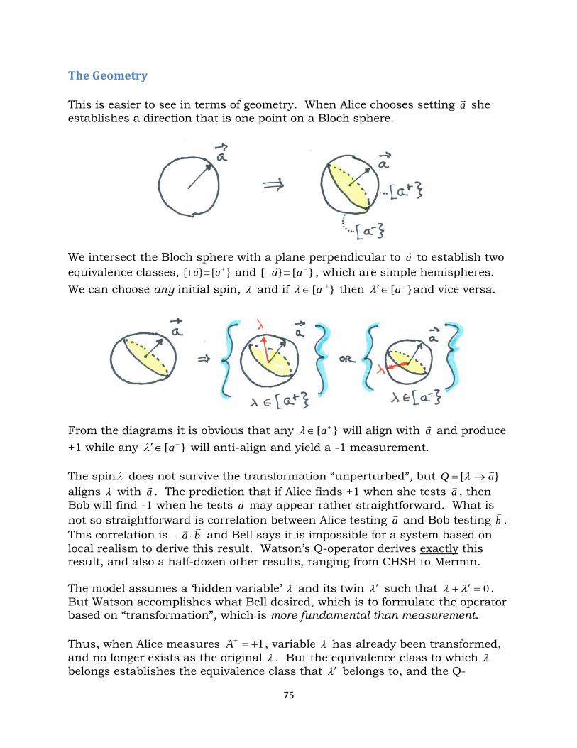
The Geometry This is easier to see in terms of geometry. When Alice chooses setting a she establishes a direction that is one point on a Bloch sphere.

We intersect the Bloch sphere with a plane perpendicular to a to establish two equivalence classes, [[ +≡+ aa and [[ −≡− aa , which are simple hemispheres. We can choose any initial spin, λ and if [ +∈ aλ then [ −∈′ aλ and vice versa.

From the diagrams it is obvious that any [ +∈ aλ will align with a and produce +1 while any [ −∈′ aλ will anti-align and yield a -1 measurement. The spinλ does not survive the transformation “unperturbed”, but [ aQ

→= λ aligns λ with a . The prediction that if Alice finds +1 when she tests a , then Bob will find -1 when he tests a may appear rather straightforward. What is not so straightforward is correlation between Alice testing a and Bob testing b

.

This correlation is ba⋅− and Bell says it is impossible for a system based on

local realism to derive this result. Watson’s Q-operator derives exactly this result, and also a half-dozen other results, ranging from CHSH to Mermin. The model assumes a ‘hidden variable’ λ and its twin λ′ such that 0=′+ λλ . But Watson accomplishes what Bell desired, which is to formulate the operator based on “transformation”, which is more fundamental than measurement. Thus, when Alice measures 1+=+A , variable λ has already been transformed, and no longer exists as the original λ . But the equivalence class to which λ belongs establishes the equivalence class that λ′ belongs to, and the Q-

75

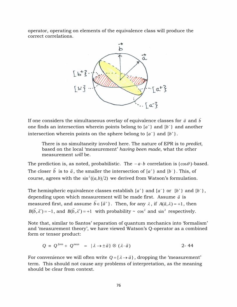
operator, operating on elements of the equivalence class will produce the correct correlations.

If one considers the simultaneous overlay of equivalence classes for a and b

one finds an intersection wherein points belong to [ +a and [ −b and another intersection wherein points on the sphere belong to [ −a and [ +b .

There is no simultaneity involved here. The nature of EPR is to predict, based on the local ‘measurement’ having been made, what the other measurement will be.

The prediction is, as noted, probabilistic. The ba ⋅− correlation is ( θcos )-based. The closer b

is to a , the smaller the intersection of [ +a and [ −b . This, of

course, agrees with the )2),((sin 2 ba we derived from Watson’s formulation. The hemispheric equivalence classes establish [ +a and [ −a or [ +b and [ −b , depending upon which measurement will be made first. Assume a is measured first, and assume [ +∈ ab

. Then, for any λ , if 1),( +=λaA , then 1),( −=′λbB

, and 1),( +=′λbB

with probability ~ 2cos and 2sin respectively. Note that, similar to Santos’ separation of quantum mechanics into ‘formalism’ and ‘measurement theory’, we have viewed Watson’s Q-operator as a combined form or tensor product: )(| aaQQQ measform

⋅⊗±→=+≡ λλ 2- 44 For convenience we will often write [ aQ

→= λ , dropping the ‘measurement’ term. This should not cause any problems of interpretation, as the meaning should be clear from context.

76

The Algebra The variable λ relates to the spin of a pristine spin one-half particle )(λp . The λ will be disturbed by sp' interaction with a Stern-Gerlach apparatus, which is represented by [ a±→λ which transforms λ into a± . The ‘hidden variable’ λ is initially random, any radius of a Bloch sphere. Alice’s measurement is: 1[),( ±=⋅±⇒⋅±→= aaaaaA λλλ . 2- 45

So that, if Bob chooses the exact opposite of Alice, then ab −= :

1)()()([[),( ±=−⋅=−⋅′→′⇒⋅′±→′=′ aaaabbbB

λλλλλ , 2- 46

in which case Alice and Bob’s measurements are perfectly correlated. The normalized Bloch sphere is

141)(

4

0

=Ω= ∫∫π

πλρλ dd 2- 47

where Ω is a unit of solid angle and πλρ 41)( = . We can now apply these definitions to Bell’s 1964 equations1.15:

If 1),( ±=aA λ ; ),(1),( bAbB

λλ −=±=′ ; 1)(∫ =λρλd (1)

Then ∫ ⋅−≠=⟩⟨ babBaAdAB ),(),()( λλλρλ (2)

Inserting Watson’s definitions into Bell’s equation (2) we obtain:

bababbaadAB⋅−=⋅±±−=⋅′±→′⋅±→Ω−=⟩⟨ ∫ )()1([[

41 4

0

λλλλπ

π

QED

From Alice’s point of view, the setting is a and the local spin is λ . Alice’s Q-operator operates only on her local particle’s spin, establishing the equivalence class ±a . Therefore the first term 1[ ±=⋅±⇒⋅±→ aaaa λλ . Next we transform the expression for Bob’s test of λ′ into local spin λ− and use this in the term representing Bob’s test: )([[ bbbb

⋅−±→′⇒⋅′±→′ λλλλ . Bob’s Q-operation

on λ′ is not local to Alice, who has already transformed her own λ to a± , so Bob’s term becomes baba

⋅=⋅±− )( , which, multiplied by 1± yields ba

⋅− , in

contradiction to Bell’s claim of impossibility. But we could have looked at the same calculation from Bob’s point of view, that is, in terms of his setting b

and of λ′ , the hidden variable tested by Bob.

1)()([),( ±=⋅±=⋅′±→′=′ bbbbbB

λλλ 2- 48

77

This establishes the equivalence class ±b describing the element of reality; we then transform Alice’s response function, a⋅λ to a⋅′− λ , so that it is described in terms of Bob’s locality. As noted, 0=′+ λλ implies that one of the variables is redundant. To focus on λ′ , we re-express λ as λ′− and reduce terms:

babbabbbadAB

⋅−=⋅±⋅=⋅′±→′⋅′−Ω=⟩⟨ ∫ )()([)(41 4

0

λλλπ

π

2- 49

Bob’s Q-operator operates only on his local particle’s spin, establishing the equivalence class ±b . Therefore Bob’s term 1[ ±=⋅±⇒⋅′±→′ bbbb

λλ . Next we

transform the expression for Alice’s test of λ into Bob’s local spin λ′− and use this in the term representing Alice’s test: )([[ aaaa

⋅′−±→⇒⋅±→ λλλλ . Alice’s Q-operation has no effect as λ is not local to Bob, who has already transformed λ′ into b

± , so Alice’s term becomes, )([ aa

⋅′−±→ λλ which, multiplied by 1± again yields ba

⋅− , contradicting Bell’s claim of impossibility.

babbaadAB⋅−⇒⋅′±→′⋅±→Ω=⟩⟨ ∫ λλλλ

π[[

41

2- 50

Thus Watson’s Q-operator or ‘jump’-operator yields the expectation value calculated by quantum mechanics found by experimental results. There is nothing “non-local” about it — Alice’s measurement is independent of Bob’s, Bob’s is independent of Alice’s. The correlation is based on the existence of locally real entities, the conserved local spins, 0=′+ λλ , and the first measure-ment, by Alice or Bob, establishes an equivalence class ±a or ±b .

Physics transforms the local spin to a local setting, and the jump operator formalism computes relevant correlations over a statistical number of tests.

Calculation of the expectation value is local. For a given pair of (twin) particles either measurement establishes an equivalence class, which determines what the other measurement will find, given only a common coordinate system linking the two remote experimental stations. There is no nonlocal physics and there is no entanglement. There is only locally real conservation of momentum until the onset of the "event" which transforms the local system from initial state )(λλ ′ to the final state determined by settings )(ba

.

Thus, Watson’s Q-operator describes the physics, produces probability distrib-utions, generates the statistical correlations and contradicts John Bell's "proof" of the impossibility of local reality models. As he himself suggested, all Bell proved was a lack of imagination. We will return to analyze the error in Bell's reasoning, after we establish further the connection to quantum mechanics.

78

The Formal Nature of the Wave Function The general quantum mechanical expansion has the form of the superposition of quantum states, nψ , with complex coefficients )(tcn :

∑∞

=

=0

)()(),(n

nn xtctx ψψ 2- 51

Unlike the general wave function, all possible spin states can be represented in a two-dimensional vector space, so we define the spin state as the expansion

⟩−+⟩+=⟩ −+ |)(|)(| tctcξ where ⟩⟨+=+ ξ|c and ⟩⟨−=− ξ|c , 2- 52 subject to normalization 1| =⟩⟨ ξξ . With this definition the squared modulus of the spin probability amplitude )(tc± is the probability that, in a measurement of the projection of spin σ at time t , we would obtain 2± . 37.478

)()(|)(|)( *2 tctctctP ±±± ==σ 2- 53 This is the physical significance (in quantum mechanics) of the expansion coefficients of the spin state ⟩ξ| . To derive the spin probability amplitude it is necessary to compute ⟩⟨ ξξ | in terms of the expansion coefficients:

)||()||(| ** −⟩++⟩⟨−+⟨+=⟩⟨ −+−+ ccccξξ 2- 54

−⟩⟨−++⟩⟨−+−⟩⟨+++⟩⟨+= −−+−−+++ |||| **** cccccccc

From the orthogonality relations jiji δ=⟩⟨ | we have: 0|| =+⟩⟨−=−⟩⟨+ , and 1|| =−⟩⟨−=+⟩⟨+ 2- 55

Therefore since 2* || ±±± = ccc

1||||| 22 =+=⟩⟨ −+ ccξξ 2- 56 which is the Born probability for the two state system. So we choose ⟩+| and

⟩−| as the two basis vectors; any state is a linear superposition of these two in a generic state: ⟩−+⟩+=⟩ −+ ||| ccξ . Thus ⟩ξ| can represent any state of spin, prepared in any manner, +c and −c are complex numbers, such that ++cc* is the probability that the spin would be measured as 1+=zσ and −−cc* the probability that the spin yields 1−=zσ , if measured. ⟩⟨+⟩+⟨=+ ξξ ||P and ⟩⟨−⟩−⟨=− ξξ ||P

79

The formulation in terms of state vectors is that if ⟩ξ| is the state vector of the system, and observable L

is measured, the probability to observe value iλ is

⟩⟨⟩⟨= ξλλξλ ||)( iiiP 2- 57

and, since 1=∑i

iP we have

1=∑i

iP ⟩⟨⟩⟨= ∑ ξλλξ |)||(| iii

2- 58

which for normalized vector ⟩iλ| implies

1|| ≡⟨⟩∑ iii

λλ , 2- 59

that is, if the system can be projected into states ⟩iλ| , the probability that it will be found in one state ⟩iλ| is certain. The mathematical formulation of quantum mechanics is quite straightforward. Nevertheless, Schrödinger’s equation is based on spatial variables ),( txψ while spin, treated as an intrinsic variable, is not. So ),( txψ , a solution of Schrödinger’s equation, contains no information about zσ , the projection of the spin onto the z-axis. But

"… the atoms ‘motion’ through space corresponds to the evolution of the wave packet according to the time-dependent Schrödinger equation –"

The phenomenally extended wave function ),,( µ trΨ might look like37.470

),,( +Ψ tr for an atom that moves up,

),,( −Ψ tr for an atom that moves down, therefore one might view the extended wave function as ),,( µ trΨ , but this is formal and the preferred extension is a product of Schrödinger’s wave function with the two-state vector ⟩−+⟩+=⟩ −+ ||| ccξ , which we can write as ),(),(),,( ttrtr µξψµ

⊗=Ψ . 2- 60 / \ )(µf≠ )(rf

≠

This extended wave function is thus a tensor product of two independent wave functions. The separability extends to spin operators and space operators, such that spin operators have no effect on spatial variables and vice versa. Therefore Schrödinger’s equation, for which the spatial wave function is a solution, has nothing that corresponds to intrinsic spin.

80

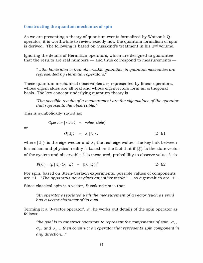
Constructing the quantum mechanics of spin As we are presenting a theory of quantum events formalized by Watson’s Q-operator, it is worthwhile to review exactly how the quantum formalism of spin is derived. The following is based on Susskind’s treatment in his 2nd volume. Ignoring the details of Hermitian operators, which are designed to guarantee that the results are real numbers — and thus correspond to measurements —

"…the basic idea is that observable quantities in quantum mechanics are represented by Hermitian operators.”

These quantum mechanical observables are represented by linear operators, whose eigenvalues are all real and whose eigenvectors form an orthogonal basis. The key concept underlying quantum theory is

"The possible results of a measurement are the eigenvalues of the operator that represents the observable."

This is symbolically stated as: ⟩=⟩ statevaluestateOperator || or ⟩=⟩ iiiO λλλ ||ˆ . 2- 61

where ⟩iλ| is the eigenvector and iλ the real eigenvalue. The key link between formalism and physical reality is based on the fact that if ⟩ξ| is the state vector of the system and observable L

is measured, probability to observe value iλ is

2|||||)( ⟩⟨≡⟩⟨⟩⟨= ξλξλλξλ iiiiP 2- 62

For spin, based on Stern-Gerlach experiments, possible values of components are 1± . “The apparatus never gives any other result." …so eigenvalues are 1± .

Since classical spin is a vector, Susskind notes that

"An operator associated with the measurement of a vector (such as spin) has a vector character of its own."

Terming it a '3-vector operator', σ , he works out details of the spin operator as follows:

"the goal is to construct operators to represent the components of spin, xσ ,

yσ , and zσ … then construct an operator that represents spin component in any direction…"

81

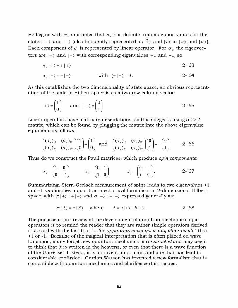
He begins with zσ and notes that zσ has definite, unambiguous values for the states ⟩+| and ⟩−| (also frequently represented as ⟩↑| and ⟩↓| or ⟩u| and ⟩d| ). Each component of σ is represented by linear operator. For zσ the eigenvec-tors are ⟩+| and ⟩−| with corresponding eigenvalues 1+ and 1− , so

⟩++=⟩+ ||zσ 2- 63

⟩−−=⟩− ||zσ with 0| =⟩−⟨+ . 2- 64 As this establishes the two dimensionality of state space, an obvious represent-ation of the state in Hilbert space is as a two-row column vector:

=⟩+

01

| and

=⟩−

10

| 2- 65

Linear operators have matrix representations, so this suggests using a 22× matrix, which can be found by plugging the matrix into the above eigenvalue equations as follows:

=

01

01

)()()()(

2221

1211

zz

zz

σσσσ

and

−=

10

10

)()()()(

2221

1211

zz

zz

σσσσ

2- 66

Thus do we construct the Pauli matrices, which produce spin components:

−

=10

01zσ

=

0110

xσ

−=

00i

iyσ . 2- 67

Summarizing, Stern-Gerlach measurement of spins leads to two eigenvalues +1 and -1 and implies a quantum mechanical formalism in 2-dimensional Hilbert space, with +⟩+=+⟩ ||σ and −⟩−=−⟩ ||σ expressed generally as:

⟩±=⟩ ξξσ || where ⟩−+⟩+= || baξ . 2- 68 The purpose of our review of the development of quantum mechanical spin operators is to remind the reader that they are rather simple operators derived in accord with the fact that “…the apparatus never gives any other result,” than +1 or -1. Because of the magical interpretation that is often placed on wave functions, many forget how quantum mechanics is constructed and may begin to think that it is written in the heavens, or even that there is a wave function of the Universe! Instead, it is an invention of man, and one that has lead to considerable confusion. Gordon Watson has invented a new formalism that is compatible with quantum mechanics and clarifies certain issues.

82

The Quantum Nature of the Wave Function We have just shown that the quantum formalism of spin is based on the 1D measurement apparatus. This was essentially built into the Uhlenbeck and Goudsmit model of the 'magnetic electron', when they hypothesized

"The projection of the intrinsic moment on any axis is quantized (and can assume one of two values)."

Thus quantum spin was born in a confused state, as no one can understand how projections on any axis can be so. In 1925, when they proposed this, Schrödinger's wave mechanics was not off the ground, and, as we have seen, must still be augmented for spin. Perhaps Bohr's quantized orbits (not under-stood either, but clearly useful for explaining spectra) had prepared physicists to accept utilitarian ideas even if they made no physical sense. Uhlenbeck and Goudsmit successfully applied the idea to the anomalous spectra of atoms in magnetic fields (which Pauli had developed the previous year.) Nevertheless, quantum spin operators were based on simulating the 1D output of such experiments, not on predicting the dynamics of spin, although we have seen that the average or expectation values of quantum spin are 'compatible' with dynamic precession, whatever is precessing. But I've also noted that the same result is compatible with no precession, i.e., alignment. Thus spin oper-ators and spin states are measurement-based and successfully predict such things as EPRB correlations, but are connected to Schrödinger's spatial wave function only tensorially. As Bell notes:

"in a complete physical theory of the type envisaged by Einstein, the hidden variable would have dynamical significance of laws of motion…"

Our laws of motion derived from the energy exchange theorem and are represented by Watsons Q-operator — [ a±→λ . But is the spin wave function properly a "law of motion"? Susskind3.94:

"The main rule – determinism – was that wherever you are in the state space, the next state is completely specified by the law of motion. […] A good law corresponds to a graph with exactly one arrow in and one arrow out at each state."

83

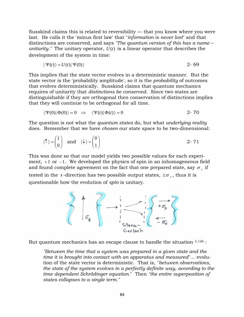
Susskind claims this is related to reversibility — that you know where you were last. He calls it the 'minus first law' that "information is never lost" and that distinctions are conserved, and says "The quantum version of this has a name – unitarity." The unitary operator, )(tU is a linear operator that describes the development of the system in time:

⟩Ψ=⟩Ψ )0(|)()(| tUt 2- 69 This implies that the state vector evolves in a deterministic manner. But the state vector is the 'probability amplitude', so it is the probability of outcomes that evolves deterministically. Susskind claims that quantum mechanics requires of unitarity that distinctions be conserved. Since two states are distinguishable if they are orthogonal then conservation of distinctions implies that they will continue to be orthogonal for all time.

⇒=⟩ΦΨ⟨ 0)0(|)0( 0)(|)( =⟩ΦΨ⟨ tt 2- 70 The question is not what the quantum states do, but what underlying reality does. Remember that we have chosen our state space to be two-dimensional:

=⟩↑

01

| and

=⟩↓

10

| 2- 71

This was done so that our model yields two possible values for each experi-ment, 1+ or 1− . We developed the physics of spin in an inhomogeneous field and found complete agreement on the fact that one prepared state, say zσ if tested in the x -direction has two possible output states, xσ± , thus it is questionable how the evolution of spin is unitary.

But quantum mechanics has an escape clause to handle the situation 3.126 :

"Between the time that a system was prepared in a given state and the time it is brought into contact with an apparatus and measured"… evolu-tion of the state vector is deterministic. That is, "between observations, the state of the system evolves in a perfectly definite way, according to the time dependent Schrödinger equation." Then "the entire superposition of states collapses to a single term."

84

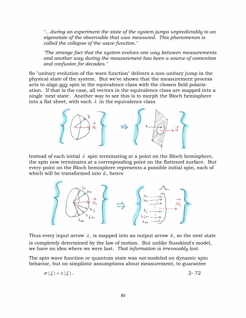
"…during an experiment the state of the system jumps unpredictably to an eigenstate of the observable that was measured. This phenomenon is called the collapse of the wave function."

"The strange fact that the system evolves one way between measurements and another way during the measurement has been a source of contention and confusion for decades."

So "unitary evolution of the wave function" delivers a non-unitary jump in the physical state of the system. But we've shown that the measurement process acts to align any spin in the equivalence class with the chosen field polariz-ation. If that is the case, all vectors in the equivalence class are mapped into a single 'next state'. Another way to see this is to morph the Bloch hemisphere into a flat sheet, with each λ in the equivalence class

Instead of each initial λ spin terminating at a point on the Bloch hemisphere, the spin now terminates at a corresponding point on the flattened surface. But every point on the Bloch hemisphere represents a possible initial spin, each of which will be transformed into a , hence

Thus every input arrow iλ is mapped into an output arrow a , so the next state is completely determined by the law of motion. But unlike Susskind's model, we have no idea where we were last. That information is irrevocably lost. The spin wave function or quantum state was not modeled on dynamic spin behavior, but on simplistic assumptions about measurement, to guarantee ⟩±=⟩ ξξσ || . 2- 72

85

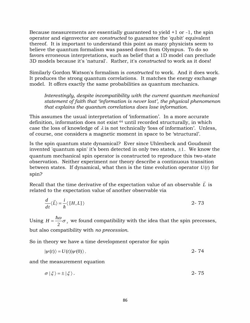
Because measurements are essentially guaranteed to yield +1 or -1, the spin operator and eigenvector are constructed to guarantee the 'qubit' equivalent thereof. It is important to understand this point as many physicists seem to believe the quantum formalism was passed down from Olympus. To do so favors erroneous interpretations, such as belief that a 1D model can preclude 3D models because it's 'natural'. Rather, it's constructed to work as it does! Similarly Gordon Watson's formalism is constructed to work. And it does work. It produces the strong quantum correlations. It matches the energy exchange model. It offers exactly the same probabilities as quantum mechanics.

Interestingly, despite incompatibility with the current quantum mechanical statement of faith that ‘information is never lost’, the physical phenomenon that explains the quantum correlations does lose information.

This assumes the usual interpretation of ‘information’. In a more accurate definition, information does not exist 44 until recorded structurally, in which case the loss of knowledge of λ is not technically ‘loss of information’. Unless, of course, one considers a magnetic moment in space to be ‘structural’.

Is the spin quantum state dynamical? Ever since Uhlenbeck and Goudsmit invented 'quantum spin' it’s been detected in only two states, 1± . We know the quantum mechanical spin operator is constructed to reproduce this two-state observation. Neither experiment nor theory describe a continuous transition between states. If dynamical, what then is the time evolution operator )(tU for spin?

Recall that the time derivative of the expectation value of an observable L is

related to the expectation value of another observable via

⟩⟨=⟩⟨ ],[ LHiLtd

d

2- 73

Using zH σω2

= we found compatibility with the idea that the spin precesses,

but also compatibility with no precession. So in theory we have a time development operator for spin

⟩=⟩ )0(|)()(| ψψ tUt , 2- 74 and the measurement equation

⟩±=⟩ ξξσ || . 2- 75

86

Is Watson’s formalism compatible with quantum mechanics? In theory, quantum mechanics provides us with two equations for spin: the time development operator equation (of the ‘ontic’ state of reality, λψ ~ )

⟩=⟩ )0(|)()(| ψψ tUt , 2- 76 and the measurement operator equation (of the ‘epistemic’ information, a±~ξ )

⟩±=⟩ ξξσ || , 2- 77 the combination of which yields the only information we have about spin. Based on this it is obvious that Watson’s Q-operator combines these two operations in a tensor product:

⟩±=⟩⊗⟩=⟩ ξξσψψ ||)0(|)()(| tUt \ | / /

aaQ ⋅⊗←±= λλ ] 2- 78

where the time evolution occurs:

λψ ~)0( →~)(tU

at ±~)(ψ

followed by measurement of the evolved spin state: 1)( ±=⋅±→⋅ aaa λ . 2- 79 Thus, whereas the quantum spin operator description of the Stern-Gerlach experiment yields 1+ or 1− , Watson’s Q-operator describes the transformation on spin and then the measurement of the final state

aaQ ⋅±→= λλ [ 2- 80

and satisfies the quantum operator equation:

⟩±=⟩ ξξ ||Q , since ⟩±=⟩⋅±=⟩⋅±→ ξξξλλ ||)(|[ aaaa 2- 81 This produces exactly the same results as the quantum correlations but does so with local realism. There is no action-at-a-distance or entanglement involved, nor is it needed. We conclude the Q-operator is fully compatible with quantum measurement theory and provides the jump-operation Bell speculated about.

87

The 'jump'-operator, Q, incorporates the physical state transition that Bell wished for in a future theory:

"The fundamental theory… would… have the [quantum] 'jumps' in the equation and not just in the talk –… It would come about as a dynamical process in dynamically defined conditions."

Our energy exchange theorem describes the relevant dynamical process, whose (classical) transformation is represented by [ a±→λ and measurement a⋅λ . But this is a generalization of quantum operators, in which the 'jump' or 'collapse of the wave function' is a not-understood process. As such, the Q-operator is not a linear operator, which must give a unique output for every vector in the space.

"the space of states for a single spin has only two dimensions." 3.37 Thus the quantum fisherman, using a 1D 'net' or Stern-Gerlach apparatus, intentionally limits the state space to two dimensions ⟩↑| and ⟩↓| .

Consequences of the Standard Formalism The consequences of this conscious choice of quantum representation is the confusion and requirement of constant caveats such as Susskind’s 3: "Complete" or "incomplete with hidden variables" – "I don't know what the

ultimate answer will be"3.37 There is something fundamentally different about the state of the quantum

system and the state of the classical system." 3.13 "If the spin really is a vector, it is a very peculiar one indeed." 3.9

"Exactly what is precessing?"3.119

In fact, exploring the case of measuring xσ followed by yσ versus yσ followed by xσ , Susskind (and most quantum physicists) conclude that "The very foundations of logic are different in quantum physics…"3.19

Different logic and no local causality – this seems a very high price to pay for removing the θ -dependence and not bothering to attempt to explain why!

88

No Epistemic Model Can Fully Explain… Recall that Leifer 31 notes

"The status of the quantum state is one of the most controversial issues in the foundation of quantum theory."

As usual, Barrett et al. begin by noting that Bell's 'no-go' theorem

"shows that locally causal models must make different predictions than quantum theory."

They then shift focus from locally causal theory to

"…whether the quantum state should be viewed as a description of the physical state of the system (an "ontic state") or as an observer’s information about the system (an "epistemic state")."

The focus recently has been on non-orthogonal states, which cannot be distinguished by single test. They choose a framework of 'ontological models', in which a physical system that has been prepared in state ⟩ψ| is assumed to be "real", or "ontic". To each quantum state is assigned an epistemic state, ψµ , which is a probability distribution over this set of ontic states Λ . The probabil-ity represents our ignorance about which ontic state Λ∈λ the system is in.

How does our model fit into the framework developed around the idea of ontic versus epistemic? The framework is typically used to propose specific types of states and seek limitations on wave functions of this type. No 'real' physical model is proposed, only generic models or types. Instead, we have developed a local model of physical reality with a formalism that does reproduce the same predictions as quantum theory. Note that the term 'state' has a nonzero overlap in these discussions. We will distinguish the 'ontic' state or real physical 'state of reality', from the 'quantum' state, or Hilbert space ‘state vector’ ⟩ψ| which may be ontic, if it represents the physical state, or epistemic if it fails to represent some aspect of reality. The quantum state ⟩ψ| represents the 'ontic' state λ by assigning an epistemic state ψµ which is a probability distribution over the set of ontic states Λ . The several meanings of state to some degree accounts for why papers on epistemic versus ontic are such a joy to read. Maroney39 treats ψ -epistemic versus ψ -ontic via non-orthogonality, the fact that "it is possible to prepare two different pure quantum states that cannot be perfectly discriminated by single ideal measurement." 39

89

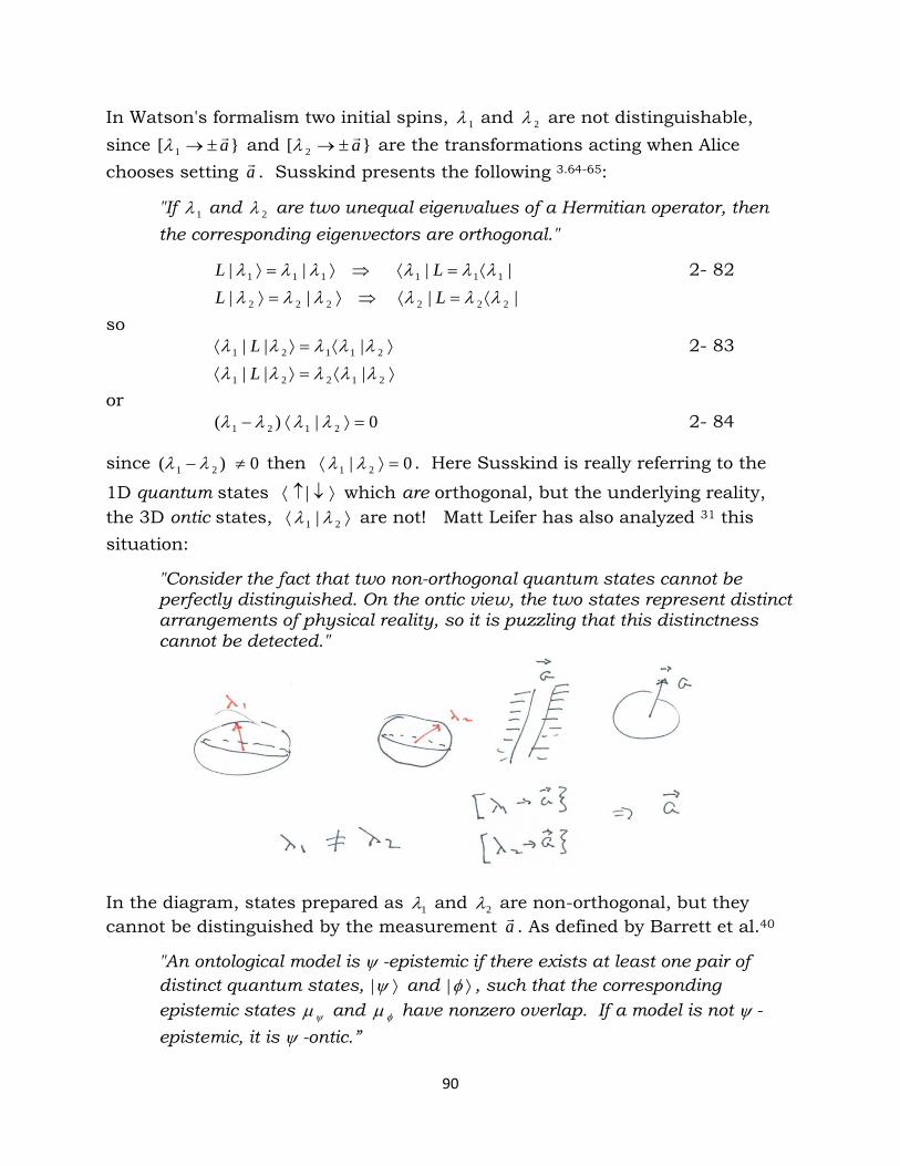
In Watson's formalism two initial spins, 1λ and 2λ are not distinguishable, since [ 1 a±→λ and [ 2 a±→λ are the transformations acting when Alice chooses setting a . Susskind presents the following 3.64-65:

"If 1λ and 2λ are two unequal eigenvalues of a Hermitian operator, then the corresponding eigenvectors are orthogonal."

⇒⟩=⟩ 111 || λλλL || 111 λλλ ⟨=⟨ L 2- 82 ⇒⟩=⟩ 222 || λλλL || 222 λλλ ⟨=⟨ L

so ⟩⟨=⟩⟨ 21121 ||| λλλλλ L 2- 83 ⟩⟨=⟩⟨ 21221 ||| λλλλλ L

or 0|)( 2121 =⟩⟨− λλλλ 2- 84

since 0)( 21 ≠− λλ then 0| 21 =⟩⟨ λλ . Here Susskind is really referring to the

1D quantum states ⟩↓↑⟨ | which are orthogonal, but the underlying reality, the 3D ontic states, ⟩⟨ 21 | λλ are not! Matt Leifer has also analyzed 31 this situation:

"Consider the fact that two non-orthogonal quantum states cannot be perfectly distinguished. On the ontic view, the two states represent distinct arrangements of physical reality, so it is puzzling that this distinctness cannot be detected."

In the diagram, states prepared as 1λ and 2λ are non-orthogonal, but they cannot be distinguished by the measurement a . As defined by Barrett et al.40

"An ontological model is ψ -epistemic if there exists at least one pair of distinct quantum states, ⟩ψ| and ⟩φ| , such that the corresponding epistemic states ψµ and φµ have nonzero overlap. If a model is not ψ -epistemic, it is ψ -ontic.”

90

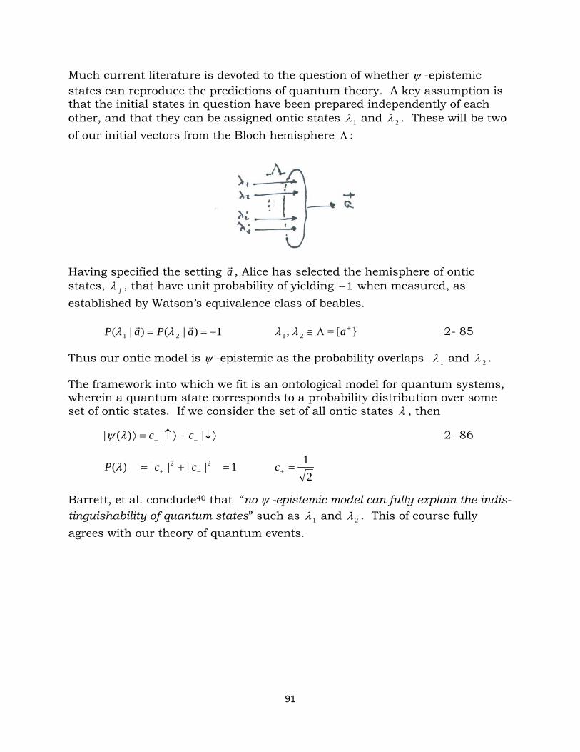
Much current literature is devoted to the question of whether ψ -epistemic states can reproduce the predictions of quantum theory. A key assumption is that the initial states in question have been prepared independently of each other, and that they can be assigned ontic states 1λ and 2λ . These will be two of our initial vectors from the Bloch hemisphere Λ :

Having specified the setting a , Alice has selected the hemisphere of ontic states, jλ , that have unit probability of yielding 1+ when measured, as established by Watson’s equivalence class of beables.

1)|()|( 21 +== aPaP λλ [, 21+≡Λ∈ aλλ 2- 85

Thus our ontic model is ψ -epistemic as the probability overlaps 1λ and 2λ . The framework into which we fit is an ontological model for quantum systems, wherein a quantum state corresponds to a probability distribution over some set of ontic states. If we consider the set of all ontic states λ , then

⟩↓+⟩↑=⟩ −+ ||)(| ccλψ 2- 86

1||||)( 22 =+= −+ ccP λ 2

1=+c

Barrett, et al. conclude40 that “no ψ -epistemic model can fully explain the indis-tinguishability of quantum states” such as 1λ and 2λ . This of course fully agrees with our theory of quantum events.

91

The Physical Nature of the Wave Function Leading edge physicists today explore many dimensions and many universes, and often attach 'magical' significance to the wave function and the equations from which it derives. For the most part they believe that quantum mechanics is fundamental; that classical mechanics emerges from statistical macroscopic averages. To return to classical physics concepts — in which continuity reigns, as physical reality, and quantum mechanics as merely a theoretical statistical model of the quantum events generated by experimental apparatus — has to be hard to take seriously for one who attaches magical significance to a formalism, but who is completely confused and perplexed about the fundamental physical reality underlying quantum mechanics, or even wonders if there is such. Recall Leifer: "the status of the quantum state is one of the most controversial issues in the foundations of quantum theory", where quantum state and wave function are almost synonymous. Is it a state of knowledge or a physically real state — is it a complete description or incomplete? Susskind simply says "I don't know what the ultimate answer will be…". One must ask why, ninety years after Schrödinger’s equation, there is so much confusion about wave functions? I suggest the ultimate answer is as follows:

The intrinsic spin is not derivable from Schrödinger’s spatial equation, whose solution is ),( trΨ . Instead the spin state ⟩)(| µξ is linked to ),( trψ as a tensor:

⟩⊗=Ψ )(|),(),,( µξψµ trtr 2- 87 Spatial derivatives operate on the spatial part, i.e. ),( trψ ; the spin operator σ operates only on ⟩ξ| . It is important to distinguish these separate aspects, which are generally associated with different momenta. The spatial part of the wave function is associated with linear momentum, p

including the rp × orbital angular momentum. It is induced by momentum

density and, in the theory of quantum events is an element of reality. The spin part of the wave function has been seen to be a ψ -epistemic function that does not directly represent an element of reality, but an equivalence class of such elements. Thus the combined wave function

⟩⊗=Ψ )(|),(),,( µξψµ trtr 2- 88 | | ψ -ontic ψ -epistemic At present I am prepared to defend the 'ψ -epistemicity' of ⟩ξ| more so than the ψ -ontic nature of ),( trψ , but a start on the ontic ),( trψ has been made in an FQXi essay: The Nature of the Wave Function. If, as I conjecture, the spatial

92

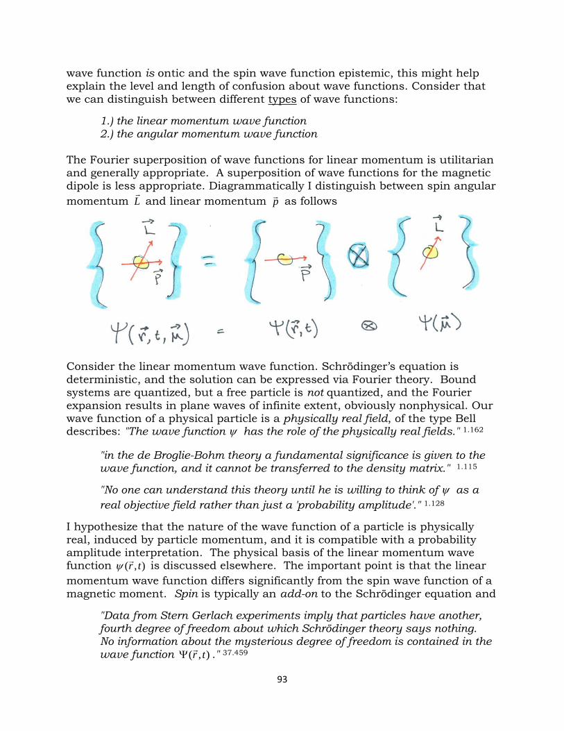
wave function is ontic and the spin wave function epistemic, this might help explain the level and length of confusion about wave functions. Consider that we can distinguish between different types of wave functions:

1.) the linear momentum wave function 2.) the angular momentum wave function

The Fourier superposition of wave functions for linear momentum is utilitarian and generally appropriate. A superposition of wave functions for the magnetic dipole is less appropriate. Diagrammatically I distinguish between spin angular momentum L

and linear momentum p as follows

Consider the linear momentum wave function. Schrödinger’s equation is deterministic, and the solution can be expressed via Fourier theory. Bound systems are quantized, but a free particle is not quantized, and the Fourier expansion results in plane waves of infinite extent, obviously nonphysical. Our wave function of a physical particle is a physically real field, of the type Bell describes: "The wave function ψ has the role of the physically real fields." 1.162

"in the de Broglie-Bohm theory a fundamental significance is given to the wave function, and it cannot be transferred to the density matrix." 1.115

"No one can understand this theory until he is willing to think of ψ as a real objective field rather than just a 'probability amplitude'." 1.128

I hypothesize that the nature of the wave function of a particle is physically real, induced by particle momentum, and it is compatible with a probability amplitude interpretation. The physical basis of the linear momentum wave function ),( trψ is discussed elsewhere. The important point is that the linear momentum wave function differs significantly from the spin wave function of a magnetic moment. Spin is typically an add-on to the Schrödinger equation and

"Data from Stern Gerlach experiments imply that particles have another, fourth degree of freedom about which Schrödinger theory says nothing. No information about the mysterious degree of freedom is contained in the wave function ),( trΨ ." 37.459

93

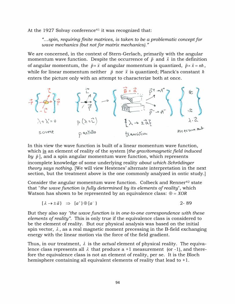
At the 1927 Solvay conference41 it was recognized that:

“…spin, requiring finite matrices, is taken to be a problematic concept for wave mechanics (but not for matrix mechanics).”

We are concerned, in the context of Stern-Gerlach, primarily with the angular momentum wave function. Despite the occurrence of p and x in the definition of angular momentum, the xp

× of angular momentum is quantized, nxp =× ,

while for linear momentum neither p nor x is quantized; Planck's constant enters the picture only with an attempt to characterize both at once.

In this view the wave function is built of a linear momentum wave function, which is an element of reality of the system [the gravitomagnetic field induced by p ], and a spin angular momentum wave function, which represents incomplete knowledge of some underlying reality about which Schrödinger theory says nothing. [We will view Hestenes’ alternate interpretation in the next section, but the treatment above is the one commonly analyzed in ontic study.] Consider the angular momentum wave function. Colbeck and Renner42 state that "the wave function is fully determined by its elements of reality", which Watson has shown to be represented by an equivalence class: XOR=⊕

[[[ −+ ⊕⇒±→ aaaλ 2- 89 But they also say "the wave function is in one-to-one correspondence with these elements of reality”. This is only true if the equivalence class is considered to be the element of reality. But our physical analysis was based on the initial spin vector, λ , as a real magnetic moment precessing in the B-field exchanging energy with the linear motion via the force of the field gradient. Thus, in our treatment, λ is the actual element of physical reality. The equiva-lence class represents all λ that produce a +1 measurement (or -1), and there-fore the equivalence class is not an element of reality, per se. It is the Bloch hemisphere containing all equivalent elements of reality that lead to +1.

94

A Geometric Algebra Perspective In geometric algebra all terms have both algebraic and geometric meaning. For example algebraically 1−=i , while every bivector B is the dual of a vector b

,

expressed as ibbiB

== where the geometric duality is expressed as multiplica-tion by the pseudoscalar i . It is generally valid to think of i as projecting out of the relevant dimension, for example

baiba

∧=× 2- 90

where ba

× is the standard vector cross product while ba

∧ is the (planar) bivector found by rotating a into b

. As an example, the electromagnetic field F

can be expressed in terms of an electric vector field E and a magnetic vector

field B

as

BiEF

+= 2- 91

which decomposes F into vector and bivector parts. In this way an electro-magnetic field ),( txFF

= with charge density ),( txρρ = and charge current ),( txJJ

= as source is determined by Maxwell's equation

Jc

Fc t

11−=

∇+∂ ρ 2- 92

which is equivalent to the standard set of four equations. It would be interesting to analyze Mansuripur’s claims in geometric algebra. In geometric algebra a bivector (2-vector) basis is spanned by

321 σσσ i= 132 σσσ i= 213 σσσ i= 2- 93

which is the bivector equivalent of the Pauli ( 22× )-matrix equation. Hestenes notes 61.28

"To describe the interaction of electron spin with an external magnetic field B

, Pauli added an interaction term to Schrödinger's equation for his two component wave function,"

Ψ⋅−Ψ=Ψ∂∂ B

mceH

ti S

σ

2 2- 94

where SH is the Schrödinger Hamiltonian and iiBB σσ =⋅ . Recall Susskind's

'momentum' ( )cAep

− and replace p with its quantum operator equivalent ∇

i and write

95

−∇−⋅=⋅ A

ceip

σσ 2- 95

and assume a Hamiltonian of the form

( ) )(21 2 xVpm

H P +⋅=σ 2- 96

and we can expand this 62.165 with )( baiIbaba

×⋅+⋅=⋅⋅ σσσ to obtain Pauli’s version of Schrodinger. After deriving this let u be the basis spin for the "spin up" eigenstate of 3σ , so we have

uu =3σ for

=

01

u or, equivalently, ⟩++=⟩+ ||3σ 2- 97

and rewrite

uiu =21σσ 2- 98

which allows us to replace 1−=i with 21σσ in Schrödinger's equation to establish a one-to-one correspondence between Pauli spinors Ψ and even multi-vectors ψ in geometric algebra, and derive the real Pauli-Schrödinger equation

33 2σψψσψ

B

mceHi

t S −=∂∂ 2- 99

where i is now the unit pseudoscalar so 321 σσσ i= . Thus, by using the geometric interpretation of i Hestenes represents spin by a bivector, which is appropriate to angular momentum, and concludes that

"Spin was originally introduced into quantum mechanics with the factor i in the original Schrödinger equation."

Hestenes then shows that the last term in the real Pauli-Schrödinger equation can be rewritten

ψµσψ Bmc

eBmce −

=−

32 2- 100

where )2(21

eei =µ and )( µµµ ×+⋅= BiBB which splits into terms proportional

to magnetic energy and torque. A physical interpretation assumes energy E of a stationary state is given by the eigenvalue equation

96

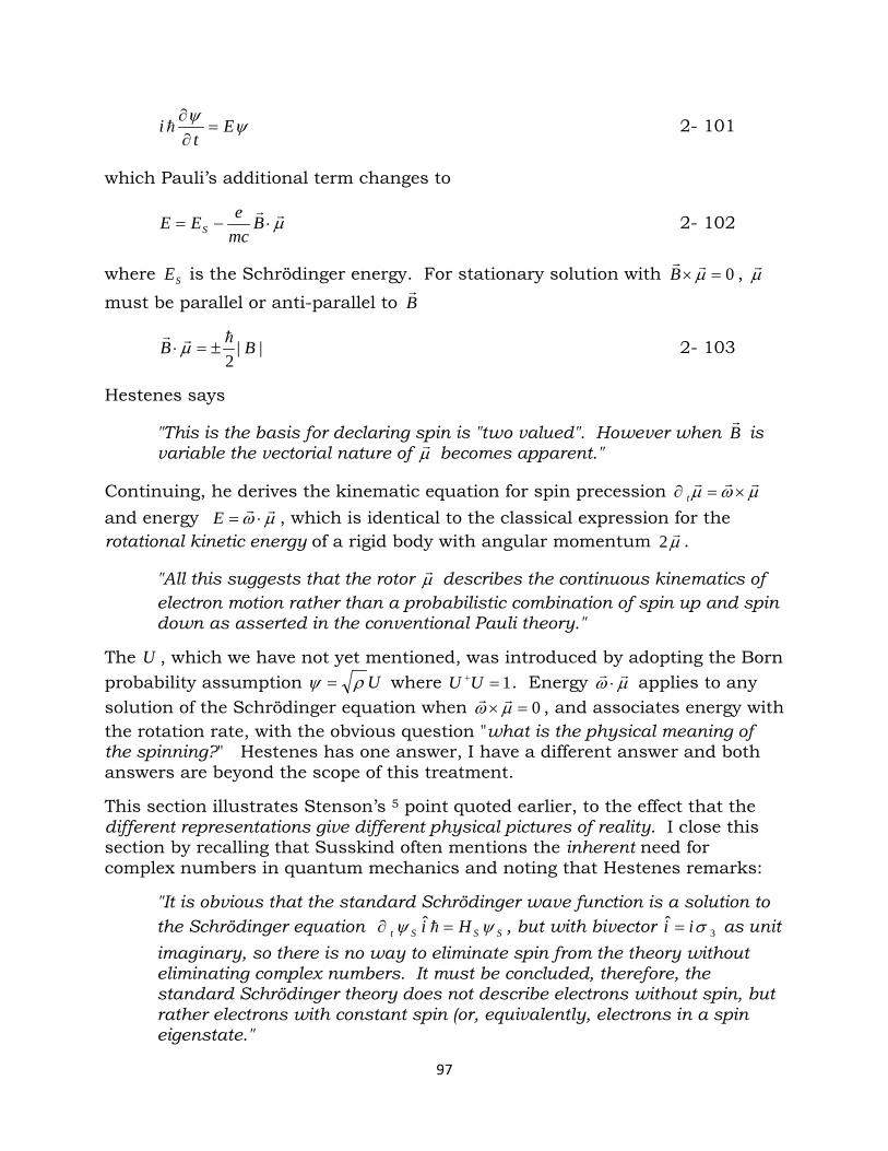
ψψ Et

i =∂∂

2- 101

which Pauli’s additional term changes to

µ⋅−= B

mceEE S 2- 102

where SE is the Schrödinger energy. For stationary solution with 0=× µB , µ

must be parallel or anti-parallel to B

||2

BB ±=⋅ µ 2- 103

Hestenes says

"This is the basis for declaring spin is "two valued". However when B

is variable the vectorial nature of µ becomes apparent."

Continuing, he derives the kinematic equation for spin precession µωµ ×=∂ t

and energy µω ⋅=E , which is identical to the classical expression for the

rotational kinetic energy of a rigid body with angular momentum µ2 .

"All this suggests that the rotor µ describes the continuous kinematics of electron motion rather than a probabilistic combination of spin up and spin down as asserted in the conventional Pauli theory."

The U , which we have not yet mentioned, was introduced by adopting the Born probability assumption Uρψ = where 1=+UU . Energy µω

⋅ applies to any solution of the Schrödinger equation when 0=× µω , and associates energy with the rotation rate, with the obvious question "what is the physical meaning of the spinning?" Hestenes has one answer, I have a different answer and both answers are beyond the scope of this treatment. This section illustrates Stenson’s 5 point quoted earlier, to the effect that the different representations give different physical pictures of reality. I close this section by recalling that Susskind often mentions the inherent need for complex numbers in quantum mechanics and noting that Hestenes remarks:

"It is obvious that the standard Schrödinger wave function is a solution to the Schrödinger equation SSSt Hi ψψ =∂ ˆ , but with bivector 3

ˆ σii = as unit imaginary, so there is no way to eliminate spin from the theory without eliminating complex numbers. It must be concluded, therefore, the standard Schrödinger theory does not describe electrons without spin, but rather electrons with constant spin (or, equivalently, electrons in a spin eigenstate."

97

Wave Function and Superposition Stern-Gerlach in 1922 were unaware of intrinsic electron spin, believing that they were testing the orbital angular momentum and consequent magnetic moment of the atoms. It was three years before Uhlenbeck and Goudsmit, based on Stern-Gerlach's experiment, in 1925 proposed 37.462 "the hypothesis of the magnetic electron" with these elements

The electron has an intrinsic magnetic moment, distinct from its orbital magnetic moment (with corresponding intrinsic angular momentum).

The projection of the intrinsic moment on any axis is quantized (and can assume one of two values, Bµ± ).

Let Hamiltonian H be partitionable into a term obsH depending only on spatial (orbital) operators and another spinH that depends only on spin operators.37.499 The hydrogen-atom-in-a-constant-field-Hamiltonian can be partitioned with

re

mpH obs

20

2

2ˆ += 2- 104

and

BH spin

⋅= σˆ 2- 105 Like all particles with spin, the spinor state functions of our system satisfy the time-dependent Schrödinger equation

),(),(ˆ trt

itrH

Ψ

∂∂

=Ψ 2- 106

But Heisenberg and Born, in 1927, noted:

“[with regard to the Uhlenbeck-Goudsmit magnetic electron] …two three dimensional wave functions are associated with each electron.”

If H can be partitioned as above, this has solutions of the separable form

=⟩=Ψ

−

+

)()(

),()(|),(),(tctc

trttrtr ψξψ 2- 107

Consider spin magnetic resonance in the case of time-dependent magnetic fields

"If a hydrogen atom is exposed to a time-varying external magnetic field zz etrBtrB ˆ),(),(

= , its Hamiltonian depends explicitly on time, so stationary states of the entire system, the atom and the field, don't exist. If the field depends on position, r , then H intermingles spatial and spin operators in such a way that there don't exist solutions to time-dependent Schrödinger equations that are separable in space and spin degrees of freedom."

98

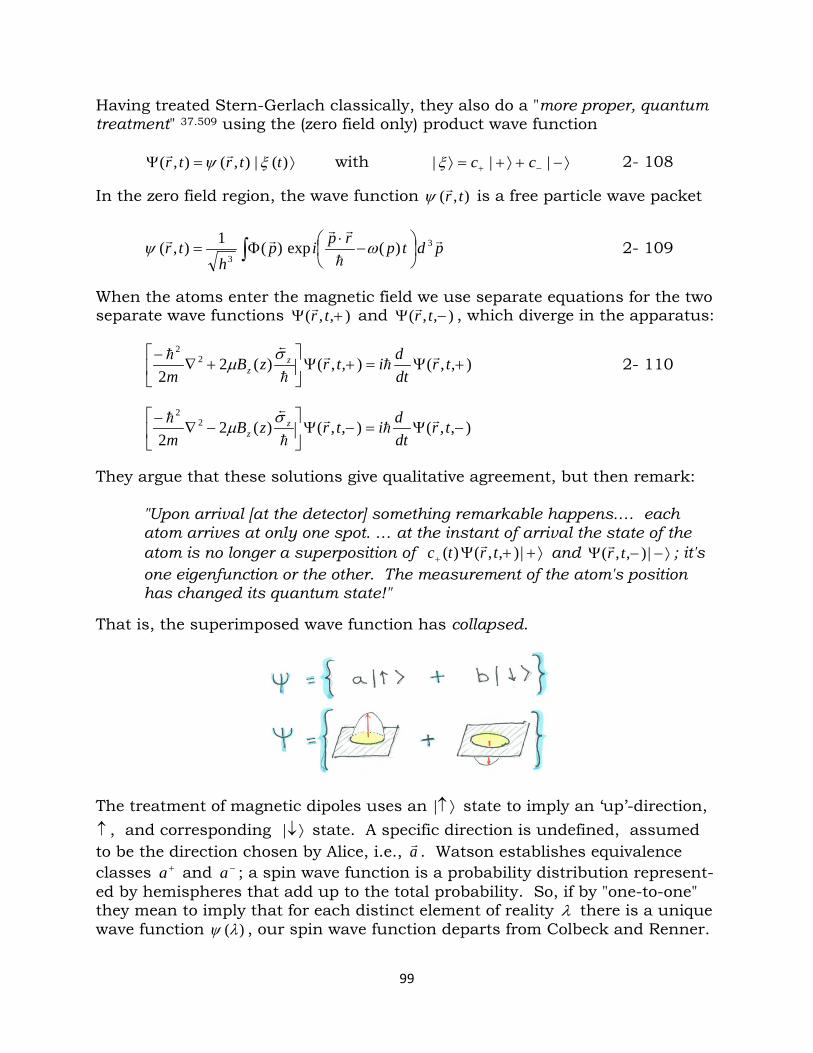
Having treated Stern-Gerlach classically, they also do a "more proper, quantum treatment" 37.509 using the (zero field only) product wave function

⟩=Ψ )(|),(),( ttrtr ξψ with ⟩−+⟩+=⟩ −+ ||| ccξ 2- 108 In the zero field region, the wave function ),( trψ is a free particle wave packet

pdtprpiph

tr

3

3)(exp)(1),(

−

⋅Φ= ∫ ωψ 2- 109

When the atoms enter the magnetic field we use separate equations for the two separate wave functions ),,( +Ψ tr and ),,( −Ψ tr , which diverge in the apparatus:

),,(),,()(22

22

+Ψ=+Ψ

+∇

− trdtditrzB

mz

z

σ

µ 2- 110

),,(),,()(22

22

−Ψ=−Ψ

−∇

− trdtditrzB

mz

z

σ

µ

They argue that these solutions give qualitative agreement, but then remark:

"Upon arrival [at the detector] something remarkable happens.… each atom arrives at only one spot. … at the instant of arrival the state of the atom is no longer a superposition of ⟩++Ψ+ |),,()( trtc and ⟩−−Ψ |),,( tr ; it's one eigenfunction or the other. The measurement of the atom's position has changed its quantum state!"

That is, the superimposed wave function has collapsed.

The treatment of magnetic dipoles uses an ⟩↑| state to imply an ‘up’-direction, ↑ , and corresponding ⟩↓| state. A specific direction is undefined, assumed to be the direction chosen by Alice, i.e., a . Watson establishes equivalence classes +a and −a ; a spin wave function is a probability distribution represent-ed by hemispheres that add up to the total probability. So, if by "one-to-one" they mean to imply that for each distinct element of reality λ there is a unique wave function )(λψ , our spin wave function departs from Colbeck and Renner.

99

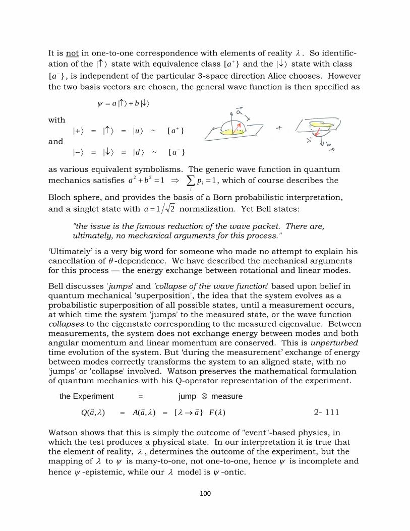
It is not in one-to-one correspondence with elements of reality λ . So identific-ation of the ⟩↑| state with equivalence class [ +a and the ⟩↓| state with class

[ −a , is independent of the particular 3-space direction Alice chooses. However the two basis vectors are chosen, the general wave function is then specified as

↓⟩+↑⟩= || baψ

with ⟩=⟩↑=⟩+ u||| [~ +a

and ⟩=⟩↓=⟩− d||| [~ −a

as various equivalent symbolisms. The generic wave function in quantum mechanics satisfies 1122 =⇒=+ ∑

iipba , which of course describes the

Bloch sphere, and provides the basis of a Born probabilistic interpretation, and a singlet state with 21=a normalization. Yet Bell states:

"the issue is the famous reduction of the wave packet. There are, ultimately, no mechanical arguments for this process."

‘Ultimately’ is a very big word for someone who made no attempt to explain his cancellation of θ -dependence. We have described the mechanical arguments for this process — the energy exchange between rotational and linear modes. Bell discusses 'jumps' and 'collapse of the wave function' based upon belief in quantum mechanical 'superposition', the idea that the system evolves as a probabilistic superposition of all possible states, until a measurement occurs, at which time the system 'jumps' to the measured state, or the wave function collapses to the eigenstate corresponding to the measured eigenvalue. Between measurements, the system does not exchange energy between modes and both angular momentum and linear momentum are conserved. This is unperturbed time evolution of the system. But ‘during the measurement’ exchange of energy between modes correctly transforms the system to an aligned state, with no 'jumps' or 'collapse' involved. Watson preserves the mathematical formulation of quantum mechanics with his Q-operator representation of the experiment. the Experiment = jump ⊗ measure )([),(),( λλλλ FaaAaQ

→== 2- 111 Watson shows that this is simply the outcome of "event"-based physics, in which the test produces a physical state. In our interpretation it is true that the element of reality, λ , determines the outcome of the experiment, but the mapping of λ to ψ is many-to-one, not one-to-one, hence ψ is incomplete and hence ψ -epistemic, while our λ model is ψ -ontic.

100

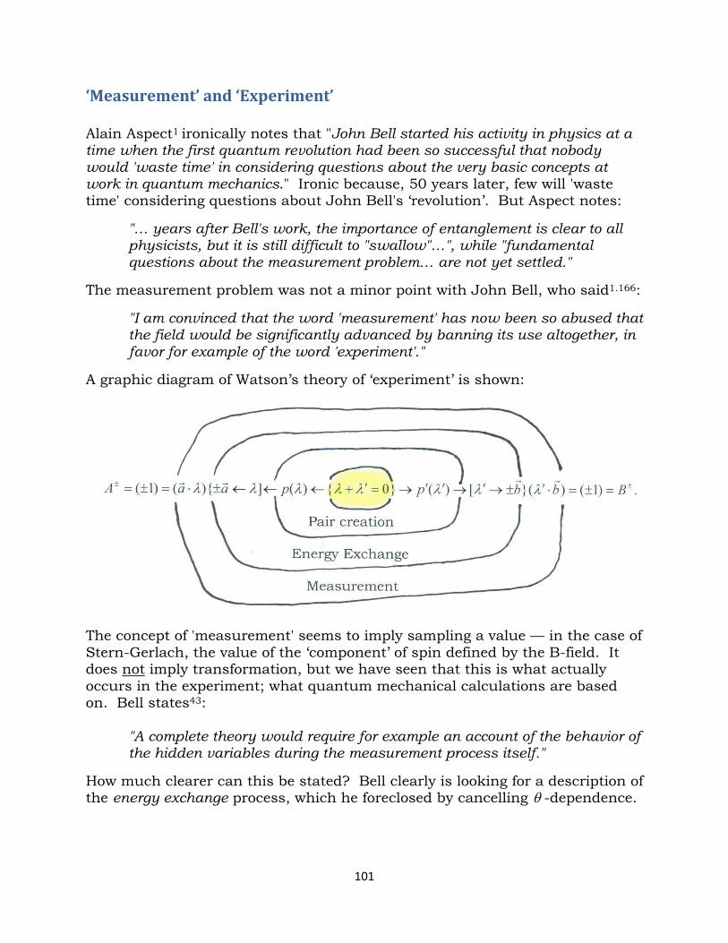
‘Measurement’ and ‘Experiment’ Alain Aspect1 ironically notes that "John Bell started his activity in physics at a time when the first quantum revolution had been so successful that nobody would 'waste time' in considering questions about the very basic concepts at work in quantum mechanics." Ironic because, 50 years later, few will 'waste time' considering questions about John Bell's ‘revolution’. But Aspect notes:

"… years after Bell's work, the importance of entanglement is clear to all physicists, but it is still difficult to "swallow"…", while "fundamental questions about the measurement problem… are not yet settled."

The measurement problem was not a minor point with John Bell, who said1.166:

"I am convinced that the word 'measurement' has now been so abused that the field would be significantly advanced by banning its use altogether, in favor for example of the word 'experiment'."

A graphic diagram of Watson’s theory of ‘experiment’ is shown:

The concept of 'measurement' seems to imply sampling a value — in the case of Stern-Gerlach, the value of the ‘component’ of spin defined by the B-field. It does not imply transformation, but we have seen that this is what actually occurs in the experiment; what quantum mechanical calculations are based on. Bell states43:

"A complete theory would require for example an account of the behavior of the hidden variables during the measurement process itself."

How much clearer can this be stated? Bell clearly is looking for a description of the energy exchange process, which he foreclosed by cancelling θ -dependence.

101

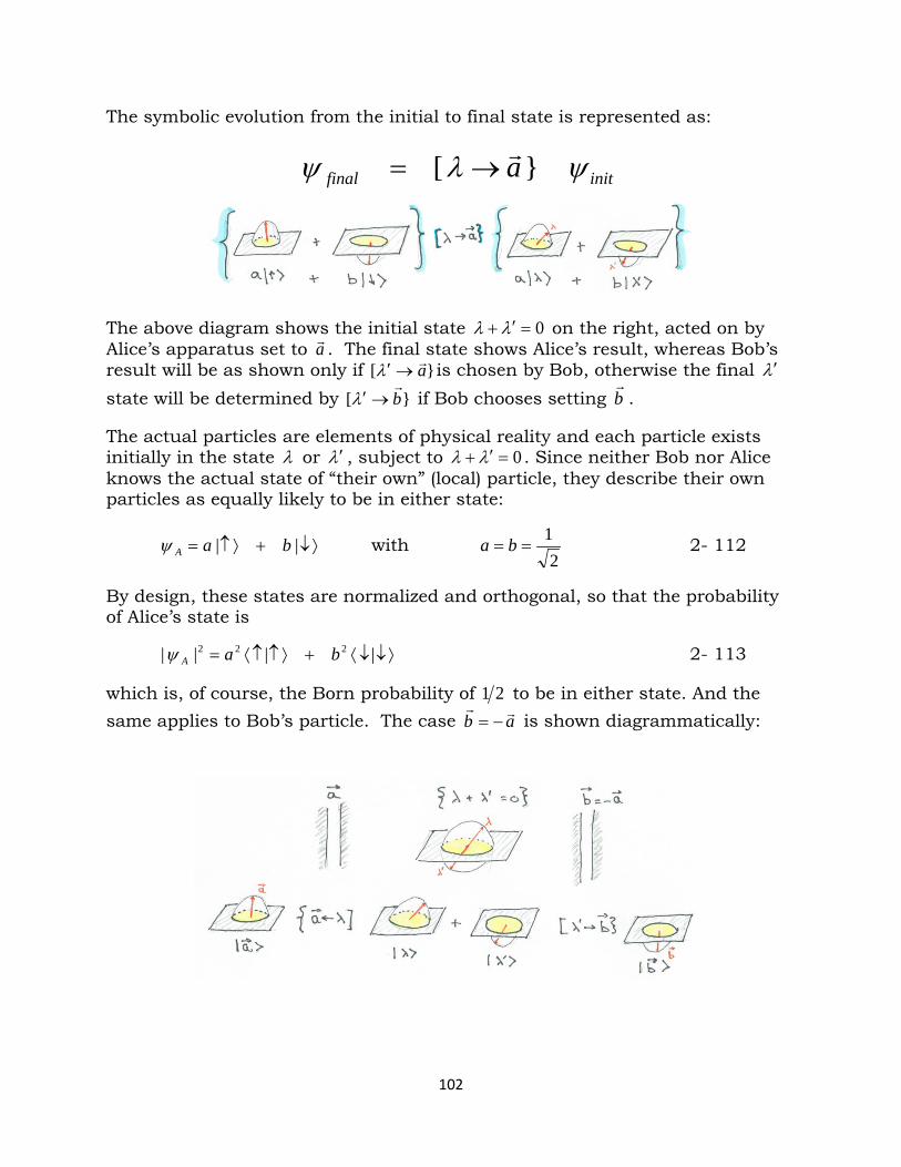
The symbolic evolution from the initial to final state is represented as:

initfinal a ψλψ [ →=

The above diagram shows the initial state 0=′+ λλ on the right, acted on by Alice’s apparatus set to a . The final state shows Alice’s result, whereas Bob’s result will be as shown only if [ a→′λ is chosen by Bob, otherwise the final λ′ state will be determined by [ b

→′λ if Bob chooses setting b

.

The actual particles are elements of physical reality and each particle exists initially in the state λ or λ′ , subject to 0=′+ λλ . Since neither Bob nor Alice knows the actual state of “their own” (local) particle, they describe their own particles as equally likely to be in either state:

⟩↓+⟩↑= || baAψ with 2

1== ba 2- 112

By design, these states are normalized and orthogonal, so that the probability of Alice’s state is

⟩↓↓⟨+⟩↑↑⟨= |||| 222 baAψ 2- 113

which is, of course, the Born probability of 21 to be in either state. And the same applies to Bob’s particle. The case ab

−= is shown diagrammatically:

102

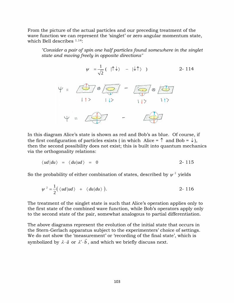
From the picture of the actual particles and our preceding treatment of the wave function we can represent the ‘singlet’ or zero angular momentum state, which Bell describes 1.14:

"Consider a pair of spin one half particles found somewhere in the singlet state and moving freely in opposite directions"

)||(2

1⟩↑↓−⟩↓↑=ψ 2- 114

In this diagram Alice’s state is shown as red and Bob’s as blue. Of course, if the first configuration of particles exists ( in which Alice = ↑ and Bob = ↓ ), then the second possibility does not exist; this is built into quantum mechanics via the orthogonality relations: 0|| =⟩⟨=⟩⟨ udduduud 2- 115 So the probability of either combination of states, described by 2ψ yields

( )⟩⟨+⟩⟨= duduudud ||212ψ . 2- 116

The treatment of the singlet state is such that Alice’s operation applies only to the first state of the combined wave function, while Bob’s operators apply only to the second state of the pair, somewhat analogous to partial differentiation. The above diagrams represent the evolution of the initial state that occurs in the Stern-Gerlach apparatus subject to the experimenters’ choice of settings. We do not show the ‘measurement’ or ‘recording of the final state’, which is symbolized by a⋅λ or b

⋅′λ , and which we briefly discuss next.

103

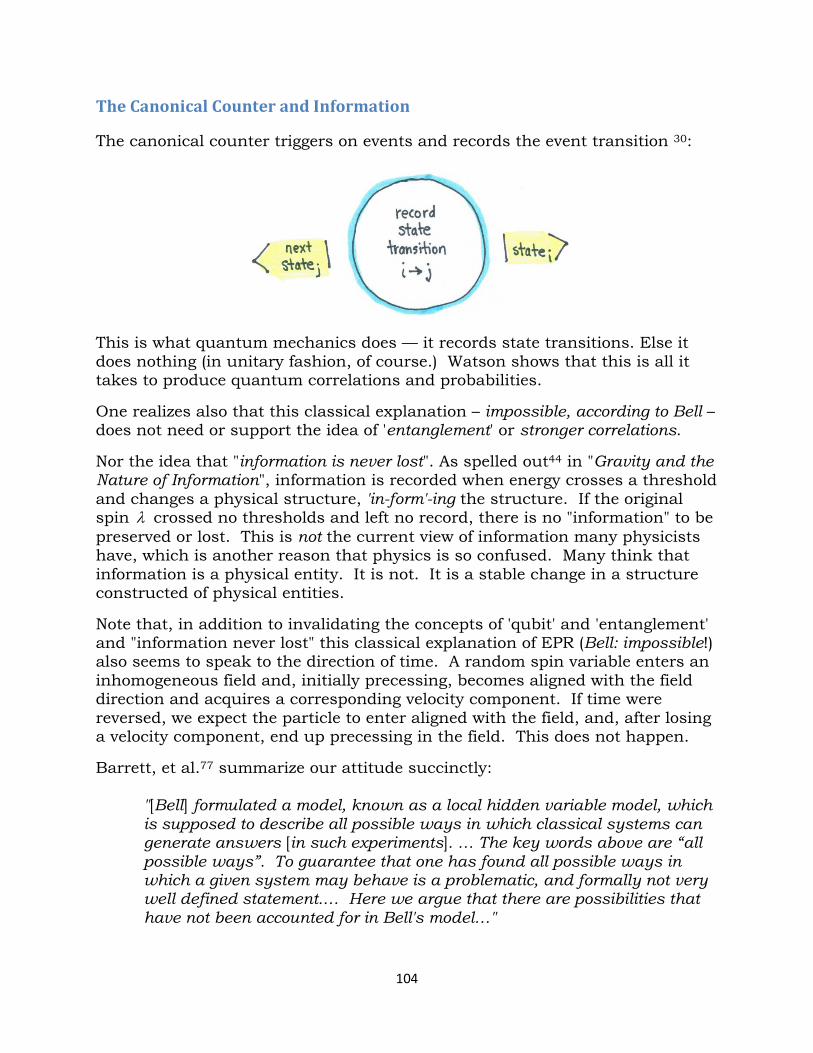
The Canonical Counter and Information The canonical counter triggers on events and records the event transition 30:

This is what quantum mechanics does — it records state transitions. Else it does nothing (in unitary fashion, of course.) Watson shows that this is all it takes to produce quantum correlations and probabilities.

One realizes also that this classical explanation – impossible, according to Bell – does not need or support the idea of 'entanglement' or stronger correlations. Nor the idea that "information is never lost". As spelled out44 in "Gravity and the Nature of Information", information is recorded when energy crosses a threshold and changes a physical structure, 'in-form'-ing the structure. If the original spin λ crossed no thresholds and left no record, there is no "information" to be preserved or lost. This is not the current view of information many physicists have, which is another reason that physics is so confused. Many think that information is a physical entity. It is not. It is a stable change in a structure constructed of physical entities.

Note that, in addition to invalidating the concepts of 'qubit' and 'entanglement' and "information never lost" this classical explanation of EPR (Bell: impossible!) also seems to speak to the direction of time. A random spin variable enters an inhomogeneous field and, initially precessing, becomes aligned with the field direction and acquires a corresponding velocity component. If time were reversed, we expect the particle to enter aligned with the field, and, after losing a velocity component, end up precessing in the field. This does not happen.

Barrett, et al.77 summarize our attitude succinctly:

"[Bell] formulated a model, known as a local hidden variable model, which is supposed to describe all possible ways in which classical systems can generate answers [in such experiments]. … The key words above are “all possible ways”. To guarantee that one has found all possible ways in which a given system may behave is a problematic, and formally not very well defined statement.… Here we argue that there are possibilities that have not been accounted for in Bell's model…"

104

Summary: Quantum Theory of Events Colin Stuart, in an FQXi article35, 'Why Quantum?', notes that

"Physicists always strive to ground their theories in aspects of physical reality … the phenomena associated with quantum physics can be derived from abstract mathematical postulates, but not from physical ones."

We, of course, have anchored our quantum theory of events in the physical reality of electron spin and magnetic fields, and, using Watson’s Q-operator formalism, we have shown how (and why) quantum theory works for spin. It works by designing systems with unique states that can be put in one-to-one correspondence with vectors in an appropriate Hilbert space. By abstracting the physical transformation involved in the experiment and presuming a naïve (i.e. non-transforming) measurement process, the system is forced into one of the fixed number of possible output states. These results are either assumed a priori equal or distributed according to a partition function, derived essentially from counting partitions containing the results. Stuart notes that

"any theory worthy of replacing quantum mechanics would still need to assign probabilities to the outcomes of experiments…"

We abstract away most of the physics, to focus on probable distributions. We use ψ -epistemic states that are information-based and therefore superimpose all possible states in a probabilistic expression with coefficients ic as shown:

⟩=⟩Ψ ∑j

jjc ψ|| 2- 117

To many physicists this looks mysterious, and even more so the fact that the

2|| ic can be interpreted as Born probabilities. But by orthogonalizing and normalizing the (Hilbert) vector space, we always obtain ∑ =

iic 1|| 2 when we

calculate ⟩ΨΨ⟨ | . The trick is to design experiments with discrete outputs ⟩iψ| and then to determine the coefficients, based on a reasonable probability distribution. Note that design includes accidental, as well as intentional. Barrett, in the same article, is quoted saying that this most successful theory – quantum mechanics – is odd, in that physicists cannot use the theory to calculate the precise outcome of quantum experiments before they've been performed, but only the probabilities for getting a certain result. But this is easy to understand in Stern-Gerlach, where the reasonable choice of the 2D Hilbert space captures the fact that measurements always yield one of two results; 1+ or 1− . Thus, given equal a priori probability, the probability of a random initial state producing either result is one half.

105

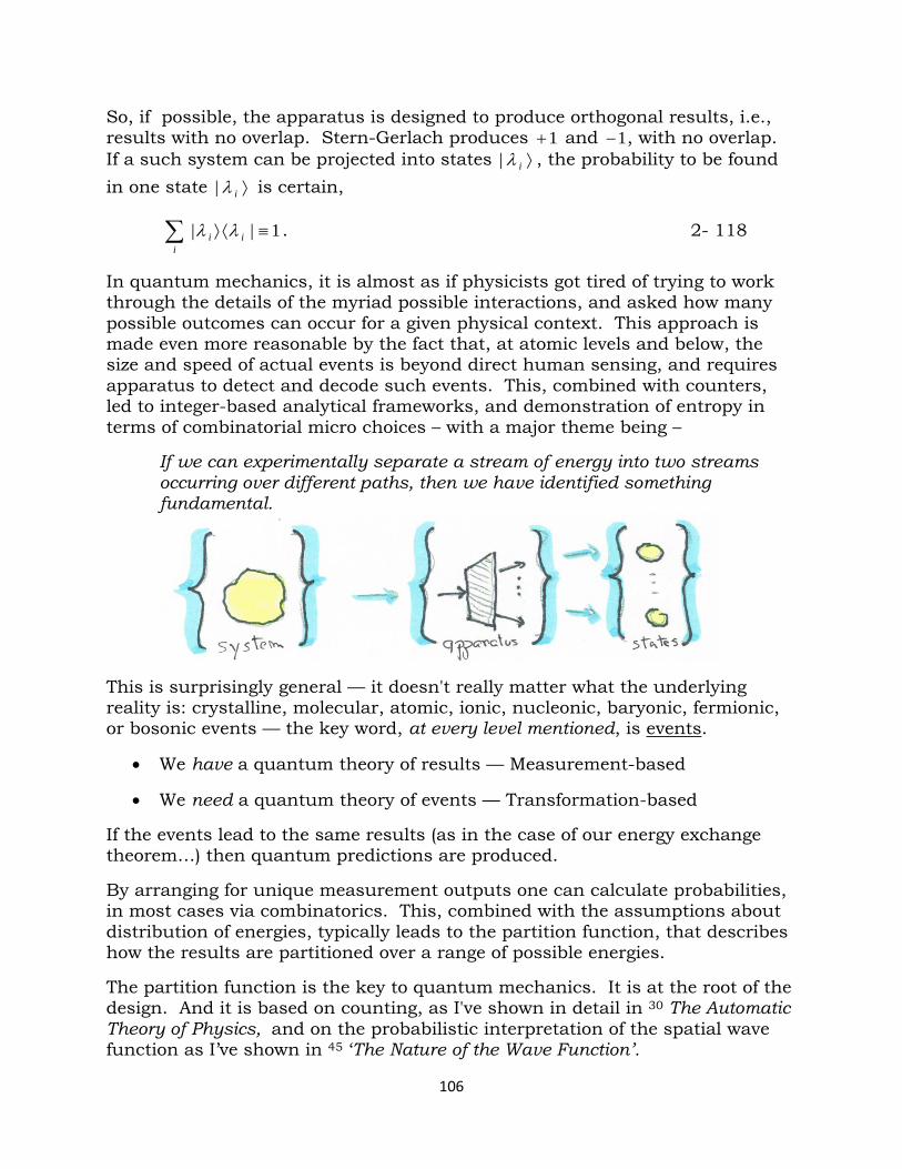
So, if possible, the apparatus is designed to produce orthogonal results, i.e., results with no overlap. Stern-Gerlach produces 1+ and 1− , with no overlap. If a such system can be projected into states ⟩iλ| , the probability to be found in one state ⟩iλ| is certain,

1|| ≡⟨⟩∑ iii

λλ . 2- 118

In quantum mechanics, it is almost as if physicists got tired of trying to work through the details of the myriad possible interactions, and asked how many possible outcomes can occur for a given physical context. This approach is made even more reasonable by the fact that, at atomic levels and below, the size and speed of actual events is beyond direct human sensing, and requires apparatus to detect and decode such events. This, combined with counters, led to integer-based analytical frameworks, and demonstration of entropy in terms of combinatorial micro choices – with a major theme being –

If we can experimentally separate a stream of energy into two streams occurring over different paths, then we have identified something fundamental.

This is surprisingly general — it doesn't really matter what the underlying reality is: crystalline, molecular, atomic, ionic, nucleonic, baryonic, fermionic, or bosonic events — the key word, at every level mentioned, is events.

• We have a quantum theory of results — Measurement-based

• We need a quantum theory of events — Transformation-based If the events lead to the same results (as in the case of our energy exchange theorem…) then quantum predictions are produced. By arranging for unique measurement outputs one can calculate probabilities, in most cases via combinatorics. This, combined with the assumptions about distribution of energies, typically leads to the partition function, that describes how the results are partitioned over a range of possible energies. The partition function is the key to quantum mechanics. It is at the root of the design. And it is based on counting, as I've shown in detail in 30 The Automatic Theory of Physics, and on the probabilistic interpretation of the spatial wave function as I’ve shown in 45 ‘The Nature of the Wave Function’.

106

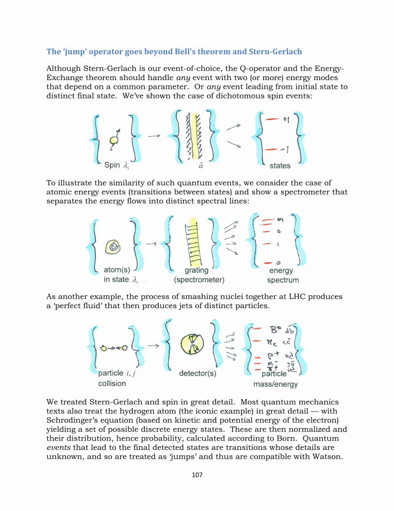
The ‘jump’ operator goes beyond Bell's theorem and Stern-Gerlach Although Stern-Gerlach is our event-of-choice, the Q-operator and the Energy-Exchange theorem should handle any event with two (or more) energy modes that depend on a common parameter. Or any event leading from initial state to distinct final state. We’ve shown the case of dichotomous spin events:

To illustrate the similarity of such quantum events, we consider the case of atomic energy events (transitions between states) and show a spectrometer that separates the energy flows into distinct spectral lines:

As another example, the process of smashing nuclei together at LHC produces a ‘perfect fluid’ that then produces jets of distinct particles.

We treated Stern-Gerlach and spin in great detail. Most quantum mechanics texts also treat the hydrogen atom (the iconic example) in great detail — with Schrodinger’s equation (based on kinetic and potential energy of the electron) yielding a set of possible discrete energy states. These are then normalized and their distribution, hence probability, calculated according to Born. Quantum events that lead to the final detected states are transitions whose details are unknown, and so are treated as ‘jumps’ and thus are compatible with Watson.

107

Less obvious, perhaps, is the case of particle energy (mass) states deriving from particle collisions which produce a ‘perfect fluid’ that then produces jets of discrete particles. The current state is described by Adare, et al.46:

“… quark-gluon plasma (GQP), a state of nuclear matter in which quarks and gluons are deconfined, is produced in nuclear collisions at sufficiently high energy. Once formed, the QGP expands, cools, and then freezes out into a collection of final-state particles. …a detailed space-time picture of the evolution of the QGP is emerging, but…”

Physicists have no model of behavior for this fluid leading to the production of elementary particles, so they jump over this process and go straight to the final result, using quantum field theory to “create” the measured result and a formal canonical counter ∑ +

ii aa to count the final states (particles). The pretense is that the different quantum fields, interacting at a point, create point particles. The reality is colorfully described above: "expands, cools, and then freezes out".

For a classical gravito-hydro-dynamics model of how the transition states of a perfect fluid create particle jets, see The Chromodynamics War 55.

Watson’s [ ip→λ represents a jump from the perfect fluid process λ to particle

ip , and quantum formalism is retained. Any quantum process that ‘jumps’ to a final state on measurement — ignoring transition behavior and treating it as merely probabilistic of various outcomes — is compatible with a jump operator.

So ‘jumps’ map into QFT and QCD, in which transitions resulting in particle creation are ignored, and only the results detected.

The probabilities are not calculated, but derived as ‘branching fractions’ from experiments. In fact, Pickering points out 78.106 that

"The 'properties' count [ for particles and resonances ] is almost entirely made up of 'branching ratios."

And Weinberg 78.181 states:

"… None of these theories is sufficiently natural.… the models all contain small parameters, such as µmme … which …ought to be calculated in any fundamental theory, which existing theories have to be put in by hand…"

This makes sense when it is realized that quantum physicists largely design experiments to yield discrete outputs, and quantum theory is largely based on mapping outputs to orthonormal state vectors compatible with Born probability. Of course these ideas carry over into the continuous energy-momentum realm, but they are essentially variations on the quantum spin formalism we derived herein. Key to quantum mechanics is the complete ignorance of the details of the transitions known as ‘jumps’ and as ‘collapse of the wave function’. This is why outputs are not predicted, but only described statistically.

108

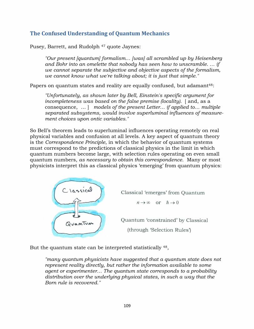
The Confused Understanding of Quantum Mechanics Pusey, Barrett, and Rudolph 47 quote Jaynes:

"Our present [quantum] formalism… [was] all scrambled up by Heisenberg and Bohr into an omelette that nobody has seen how to unscramble. … if we cannot separate the subjective and objective aspects of the formalism, we cannot know what we're talking about; it is just that simple."

Papers on quantum states and reality are equally confused, but adamant48:

"Unfortunately, as shown later by Bell, Einstein's specific argument for incompleteness was based on the false premise (locality). [ and, as a consequence, … ] models of the present Letter… if applied to… multiple separated subsystems, would involve superluminal influences of measure-ment choices upon ontic variables."

So Bell’s theorem leads to superluminal influences operating remotely on real physical variables and confusion at all levels. A key aspect of quantum theory is the Correspondence Principle, in which the behavior of quantum systems must correspond to the predictions of classical physics in the limit in which quantum numbers become large, with selection rules operating on even small quantum numbers, as necessary to obtain this correspondence. Many or most physicists interpret this as classical physics ‘emerging’ from quantum physics:

But the quantum state can be interpreted statistically 48,

"many quantum physicists have suggested that a quantum state does not represent reality directly, but rather the information available to some agent or experimenter… The quantum state corresponds to a probability distribution over the underlying physical states, in such a way that the Born rule is recovered."

109

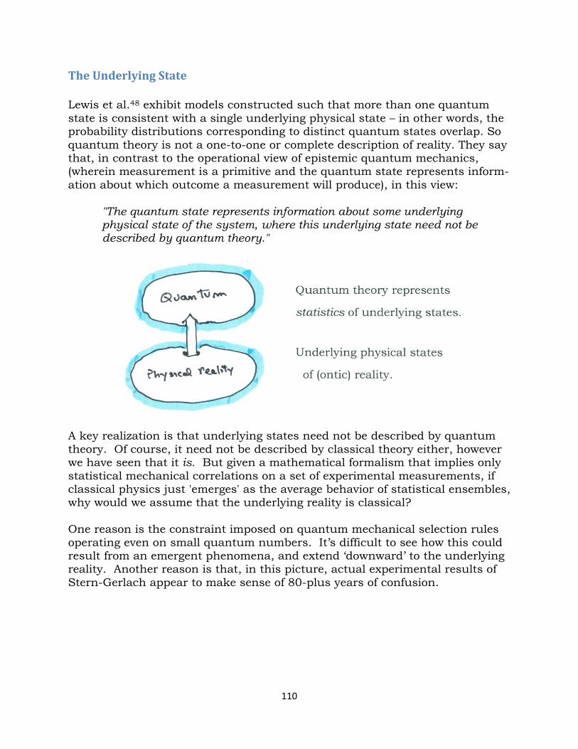
The Underlying State Lewis et al.48 exhibit models constructed such that more than one quantum state is consistent with a single underlying physical state – in other words, the probability distributions corresponding to distinct quantum states overlap. So quantum theory is not a one-to-one or complete description of reality. They say that, in contrast to the operational view of epistemic quantum mechanics, (wherein measurement is a primitive and the quantum state represents inform-ation about which outcome a measurement will produce), in this view:

"The quantum state represents information about some underlying physical state of the system, where this underlying state need not be described by quantum theory."

A key realization is that underlying states need not be described by quantum theory. Of course, it need not be described by classical theory either, however we have seen that it is. But given a mathematical formalism that implies only statistical mechanical correlations on a set of experimental measurements, if classical physics just 'emerges' as the average behavior of statistical ensembles, why would we assume that the underlying reality is classical? One reason is the constraint imposed on quantum mechanical selection rules operating even on small quantum numbers. It’s difficult to see how this could result from an emergent phenomena, and extend ‘downward’ to the underlying reality. Another reason is that, in this picture, actual experimental results of Stern-Gerlach appear to make sense of 80-plus years of confusion.

110

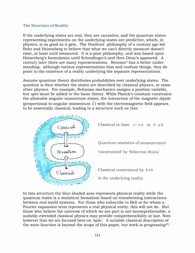
The Structure of Reality If the underlying states are real, they are causative, and the quantum states representing experiments on the underlying states are predictive, which, in physics, is as good as it gets. The Positivist philosophy of a century ago led Bohr and Heisenberg to believe that what we can’t directly measure doesn’t exist, at least until measured. It is a poor philosophy, and was based upon Heisenberg’s formulation until Schrodinger’s and then Dirac’s appeared. A century later there are many representations. Stenson5 has a better under-standing: although various representations bias and confuse things, they do point to the existence of a reality underlying the separate representations. Assume quantum theory distributes probabilities over underlying states. The question is then whether the states are described by classical physics, or some other physics. For example, Bohmian mechanics assigns a position variable, but spin must be added to the basic theory. While Planck’s constant constrains the allowable angular momentum states, the interaction of the magnetic dipole (proportional to angular momentum L

) with the electromagnetic field appears

to be essentially classical, leading to a structure such as this:

In this structure the blue shaded area represents physical reality while the quantum realm is a statistical formalism based on transforming interactions between real world systems. For those who subscribe to Bell or for whom a Fourier expansion term represents a real physical entity, this will not do. But those who believe the universe of which we are part is not incomprehensible, a suitably extended classical physics may provide comprehensibility at last. Note however that we are focused here on ‘spin’. A suitable classical description of the wave function is beyond the scope of this paper, but work is progressing45.

111

But is it realistic? But could a classical model work? Eisberg and Resnick49 on Magnetic Dipole Moments, Spin, and Transition Rates:

"Our treatments … employ a combination of simple electromagnetic theory, partly classical physics such as the Bohr model, and quantum mechanics. […] This procedure is justified by the fact that the results agree with those of completely quantum mechanical treatments." 49.291

Reinhard et al., experimentally find that 50:

"…the semi classical description is valid for large magnetic fields…"

John Bell states 1.238

"the notion of external field is more honorable than that of 'measurement'. There are many cases in practice where our electromagnetic field can be considered, in an adequate approximation, to be classical and external to the quantum system."

We found that transformation of rotational energy into linear energy occurring when the atom travels through the changing field is compatible with Maxwell’s equations and Mansuripur’s conservation of angular momentum via Einstein-Laub’s formula augmented by an expression for torque density. He concludes that the nature of electric and magnetic dipoles is such that their interactions with electromagnetic fields

"… are governed by the [torsion-augmented Einstein-Laub] equations when linear and angular momentum are being exchanged",

And recall the spin magnetic resonance case of time-dependent magnetic fields:

"If a hydrogen atom is exposed to a time-varying external magnetic field … that depends on position r , then H intermingles spatial and spin operators in such a way that there don't exist solutions to time-dependent Schröd-inger equations that are separable in space and spin degrees of freedom."

Our energy-exchange theorem argues against Bell and Susskind and all of the standard magical quantum mechanical interpretations of Stern-Gerlach. But Bell, in a section on quantum entanglement 1.204 said:

"There is nothing in this theory but the wave function." On the other hand, he states1.241 that

"Most physicists do not really accept, deep down, that the wave function is the whole story."

112

Remember what’s at stake Just to recall how confused current quantum mechanics is 52:

"A particle emerges from the source and travels towards the screen. The spin of the particle, at time 0=t , is in the superposition state of pointing "up" +⟩| and pointing "down" ⟩−| . It can be represented by ⟩−++⟩=⟩= ||0| bat As it passes through the magnets, the "up" component of the spin pulls the particle up, and the "down" component of the spin pulls it down. As a result, the particle becomes "fuzzy" and splits with the superposition of two wave packets traveling in different directions – simultaneously in two positions. When this superposition of wave packets, on reaching the other end, interacts with the detectors, quantum coherence is destroyed, and the particle is detected at one of the two positions (with probability 2|~|)( aupP and 2|~|)( bdownP . This last stage, where the superposition of the two wave packets is destroyed, and one ends up with the particle either ‘here’ or ‘there’, is loosely referred to as the wave function collapse."

That, as I understand it, is a not uncommon interpretation of the Copenhagen Interpretation of quantum mechanics. But there are others; in "Can a Future Choice Affect a Past Measurement's Outcome?" Aharonov et al. start off with 69:

"Bell's theorem has dealt the final blow on all attempts to explain EPR correlations by invoking previously existing local hidden variables."

When one starts with this statement of faith, one can end up with their idea:

"The hidden variable would then be the future state vector, affecting weak measurements at present. Then what turns out to be nonlocal in space turns out to be perfectly local in space-time."

Of course, the a± is in the future when λ is created but why would one wish to do such a thing unless one views Bell as infallible? They also write:

"Naturally, more conservative interpretations ought to be considered before concluding that measurement’s results anticipated future event. By normal causality, it must be Alice's results which affected Bob's…"

Even without considering the ‘Many World’s Interpretation’, these two views should remind us of the confusion, and motivate an attempt to understand how Watson’s formalism and the Energy-Exchange Theorem yield a classical model that produces quantum correlations, without magic! We next pursue the question of just exactly where Bell went wrong.

113

Born Rule and Bayesian Probability Chris Fuchs explains QBism, a formulation based on 'Quantum Bayesianism". A Bayesian interpretation of probability is contrasted to a frequency-based one. Fuchs views 79 the Born Rule as an addition to the rules of probability theory. In my estimation, the overlay of probability on physics is primarily 'frequentist', based on counting various possibilities and summing all possibilities, then normalizing via this sum. The distinct ratios determine the probabilities, which automatically sum to one. This is overlaid on 'reality' by noticing that the inner product of a vector with itself ( ⟩⟨≡⋅ ψψψψ | ) can always be self-normalized via

|||| ⟩⟨⟩⟨ ψψψψ and is always expressible by ∑ =i

i 1|| 2ψ .

The Born Rule associates iψ with vectors whose components are in one-to-one correspondence with the outcomes of relevant physical events:

⟩=⟩ iii || ψψ when 0|,1| =⟩⟨=⟩⟨ jiii 2- 119 When this is overlaid on the Bayesian probability 80

)|()|()|()|()|( zxPxzyPzyPyzxPzxyP == 2- 120 we have a probabilistic formalism that works.

The problem then is to determine the probabilities ⟩⟨= ψψ |ii . This is done experimentally by counting. The number of distinct instances are counted, and the counts are associated with relevant partitions, where the problem is partitioned into more than one state. Ignoring the infinite continuous partition-ability of a free particle, the simplest case is the partitioning of the Stern-Gerlach results into two partitions, a partition counting +1 results and one counting -1 results. This is easy to establish experimentally, and to intuitively assign a 50-50 or equal a priori distribution thereto. For more complex systems, such as hydrogen energy states, the counting is more complex, but the probabilities of the various energy outcomes of events (transitions between states) are generally summarized by the rule,

"The more energy is required (involved) in a particular transition, the less frequently that transition occurs."

If a multi-particle system, composed of various discrete energies, is considered, one can count the various ways the energies can be partitioned and derive the partition function, which is the true basis of quantum mechanical probability. Fuchs notes that, despite the fact that, "In the history of physics, there has never been a healthier body than quantum theory…", nevertheless,

114

"There is something about quantum theory that is different in character from any physical theory posed before",

and many physicists, over the last century, have the continuing feeling that

“…something at the bottom of it does not make sense." He summarizes major approaches to interpreting quantum mechanics: deBroglie-Bohm ‘pilot wave’: no measurements, only 'particles' flying

around in a 3N-dimensional configuration space, pushed around by a wave function regarded as a real physical field.

Spontaneous collapse: systems are endowed with quantum states that generally evolve unitarily, but from time-to-time collapse without any need for measurement.

Everettian 'many-worlds': only the world as a whole – the 'multiverse'

exists; its quantum state evolves deterministically – probability is an illusion seen from one 'branch'.

Our Theory of Quantum Events assumes an ontic wave function, similar, but not identical to, deBroglie-Bohm and the epistemic spin function we’ve seen:

)()( µψψ epistemicontic p ⊗=Ψ 2- 121 QM fundamentalists focus on the nature of the quantum state and probability. That is what the ontic/epistemic hullabaloo is about. The nature of probability is quoted 81 by Mark Feeley: "Probability is not real". While Fuchs’ analysis of probability leads him to change the emphasis from "state of knowledge" to "degree of belief", it does not solve Bell’s problem. The QBists appear to reclaim 'locality' by relinquishing 'reality', at least in the sense of Einstein's "elements of physical reality". Nevertheless, while claiming that "quantum states must… be like personalist, Bayesian probabilities", Fuchs says:

"If one has elicited one’s degrees of belief for the outcomes of a xσ measurement and similarly one’s degrees of belief for the outcomes of yσ and zσ measurements, then this is the same as specifying a quantum state itself: for if one knows the quantum state projections onto three independent axes, then that uniquely determines a Bloch vector, and hence a quantum state."

It is this belief, as we've seen, that is a major source of confusion in QM.

115

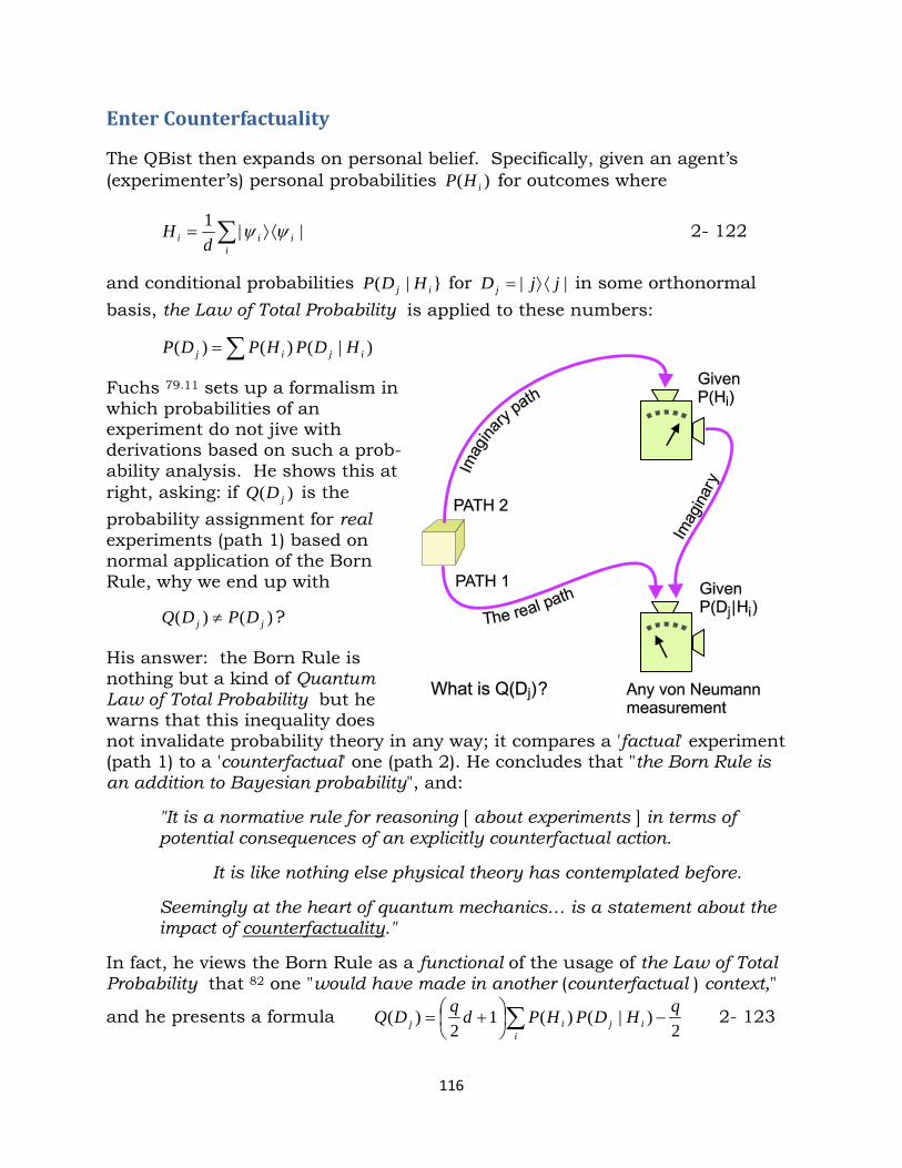
Enter Counterfactuality

The QBist then expands on personal belief. Specifically, given an agent’s (experimenter’s) personal probabilities )( iHP for outcomes where

∑ ⟨⟩=i

iii dH ||1 ψψ 2- 122

and conditional probabilities |( ij HDP for || jjD j ⟨⟩= in some orthonormal basis, the Law of Total Probability is applied to these numbers:

∑= )|()()( ijij HDPHPDP

Fuchs 79.11 sets up a formalism in which probabilities of an experiment do not jive with derivations based on such a prob-ability analysis. He shows this at right, asking: if )( jDQ is the probability assignment for real experiments (path 1) based on normal application of the Born Rule, why we end up with

)()( jj DPDQ ≠ ?

His answer: the Born Rule is nothing but a kind of Quantum Law of Total Probability but he warns that this inequality does not invalidate probability theory in any way; it compares a 'factual' experiment (path 1) to a 'counterfactual' one (path 2). He concludes that "the Born Rule is an addition to Bayesian probability", and:

"It is a normative rule for reasoning [ about experiments ] in terms of potential consequences of an explicitly counterfactual action.

It is like nothing else physical theory has contemplated before. Seemingly at the heart of quantum mechanics… is a statement about the impact of counterfactuality."

In fact, he views the Born Rule as a functional of the usage of the Law of Total Probability that 82 one "would have made in another (counterfactual ) context,"

and he presents a formula ∑ −

+=

iijij

qHDPHPdqDQ2

)|()(12

)( 2- 123

116

where d is the finite Hilbert space dimension and q takes on integer values, ∞= ...,,2,1,0q . The 2=q case is identified as quantum mechanics, while case

0=q is identified with the classical world:

"…where counterfactuals simply do not matter, for the world just ‘is’."

…a world where the fine details of the experiment don’t matter. He claims of the mathematical structure of quantum mechanics, that the formalism, per Bell's theorem, is eye-opening, and what is seen when the eyes are open is

"Non-locality everlasting… [ a world ] full of spooky action at a distance"

"That the world should violate Bell's theorem remains … the deepest statement ever drawn from quantum theory."

Unfortunately, in order to rescue locality from "non-locality everlasting", Fuchs claims that "it is the EPR criterion that should be jettisoned, not locality," where the criterion of EPR is simply stated by Einstein:

"If, without in any way disturbing a system, we can predict with certainty …the value of a physical quantity, then there exists an element of reality corresponding to that quantity."

Fuchs: "without doubt, no personalist Bayesian would ever utter such a notion", and from here Fuchs wanders off into metaphysical speculations. Focusing on the Born Rule as key to quantum mechanics, QBists apply Bayes-ian probability 82 to quantum theory. In being focused on knowledge or belief, the analysis of Bell's violation of intuition is idea-based — ideas that gravitate toward the metaphysical, which is an unlimited domain — if possible, it would be better to locate the problem in a less abstract, more physical realm.

When the hammer is Bayesian probability, the nails look like information, and the measure is belief.

When the hammer is Frequency-based probability theory, the nails look like counting, and the measure is the numeric ratio derived from physics experiments and from theoretical models.

Fuchs captures the essence of the problem: counterfactualism, and illustrates its nature graphically, showing two paths to a result — the direct path through the actual experiment and the indirect path, through counterfactual reasoning. Bayesian probability appears more likely to subscribe to ideas of superposition; all states are in the mix, yet experimental outcomes ‘collapse’ to one state. In contrast, a frequentist approach counts actual outcomes; counterfactual out-comes are not counted, as they don't exist. So frequentist quantum mechanics should correlate with reality, while the counterfactual correlates with John Bell and his "proof" that local causality cannot explain quantum correlations.

117

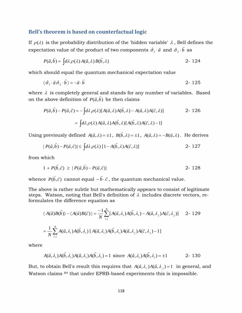
Bell’s theorem is based on counterfactual logic If )(λρ is the probability distribution of the 'hidden variable' λ , Bell defines the expectation value of the product of two components a⋅1σ and b

⋅2σ as

∫= ),(),()(),( λλλρλ bBaAdbaP 2- 124

which should equal the quantum mechanical expectation value

baba⋅−=⟩⋅⋅⟨ 21 ˆˆ σσ 2- 125

where λ is completely general and stands for any number of variables. Based on the above definition of ),( baP

he then claims

∫ −−=− )],(),(),(),([)(),(),( λλλλλρλ cAaAbAaAdcaPbaP 2- 126

∫ −= ]1),(),([),(),()( λλλλλρλ cAbAbAaAd

Using previously defined 1),( ±=λaA , 1),( ±=λbB

, ),(),( λλ aBaA −= . He derives

∫ −≤− )],(),(1[)(|),(),(| λλλρλ cAbAdcaPbaP 2- 127 from which

|),(),(|),(1 caPbaPcbP −≥+ 2- 128

whence ),( cbP cannot equal cb ⋅− , the quantum mechanical value.

The above is rather subtle but mathematically appears to consist of legitimate steps. Watson, noting that Bell's definition of λ includes discrete vectors, re-formulates the difference equation as

∑ −−

=⟩⟨−⟩⟨N

jijjii cAaAbAaA

NcBaAbBaA

,)],(),(),(),([1)()()()( λλλλ 2- 129

∑ −=N

jijjiiii cAaAbAaAbAaA

N ,]1),(),(),(),([),(),(1 λλλλλλ

where

1),(),(),(),( =iiii bAaAbAaA λλλλ since 1),(),( ±=ii bAaA λλ

2- 130

But, to obtain Bell's result this requires that 1),(),( =ji aAaA λλ in general, and Watson claims 84 that under EPRB-based experiments this is impossible.

118

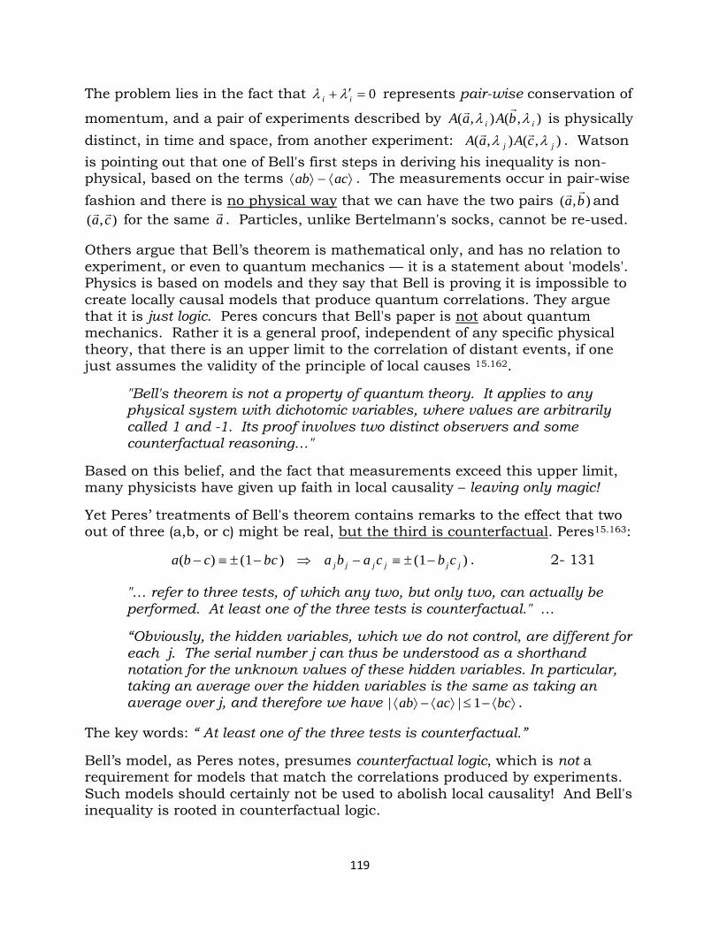
The problem lies in the fact that 0=′+ ii λλ represents pair-wise conservation of

momentum, and a pair of experiments described by ),(),( ii bAaA λλ is physically

distinct, in time and space, from another experiment: ),(),( jj cAaA λλ . Watson is pointing out that one of Bell's first steps in deriving his inequality is non-physical, based on the terms ⟩⟨−⟩⟨ acab . The measurements occur in pair-wise fashion and there is no physical way that we can have the two pairs ),( ba

and ),( ca for the same a . Particles, unlike Bertelmann's socks, cannot be re-used.

Others argue that Bell’s theorem is mathematical only, and has no relation to experiment, or even to quantum mechanics — it is a statement about 'models'. Physics is based on models and they say that Bell is proving it is impossible to create locally causal models that produce quantum correlations. They argue that it is just logic. Peres concurs that Bell's paper is not about quantum mechanics. Rather it is a general proof, independent of any specific physical theory, that there is an upper limit to the correlation of distant events, if one just assumes the validity of the principle of local causes 15.162.

"Bell's theorem is not a property of quantum theory. It applies to any physical system with dichotomic variables, where values are arbitrarily called 1 and -1. Its proof involves two distinct observers and some counterfactual reasoning…"

Based on this belief, and the fact that measurements exceed this upper limit, many physicists have given up faith in local causality – leaving only magic!

Yet Peres’ treatments of Bell's theorem contains remarks to the effect that two out of three (a,b, or c) might be real, but the third is counterfactual. Peres15.163:

)1()1()( jjjjjj cbcabacbcba −±≡−⇒−±≡− . 2- 131

"… refer to three tests, of which any two, but only two, can actually be performed. At least one of the three tests is counterfactual." … “Obviously, the hidden variables, which we do not control, are different for each j. The serial number j can thus be understood as a shorthand notation for the unknown values of these hidden variables. In particular, taking an average over the hidden variables is the same as taking an average over j, and therefore we have ⟩⟨−≤⟩⟨−⟩⟨ bcacab 1|| .

The key words: “ At least one of the three tests is counterfactual.”

Bell’s model, as Peres notes, presumes counterfactual logic, which is not a requirement for models that match the correlations produced by experiments. Such models should certainly not be used to abolish local causality! And Bell's inequality is rooted in counterfactual logic.

119

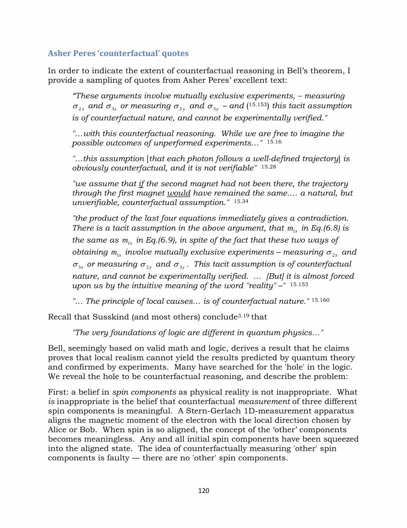
Asher Peres ‘counterfactual’ quotes In order to indicate the extent of counterfactual reasoning in Bell’s theorem, I provide a sampling of quotes from Asher Peres’ excellent text:

“These arguments involve mutually exclusive experiments, – measuring x2σ and x3σ or measuring y2σ and y3σ – and (15.153) this tacit assumption

is of counterfactual nature, and cannot be experimentally verified."

"…with this counterfactual reasoning. While we are free to imagine the possible outcomes of unperformed experiments…" 15.16 "…this assumption [that each photon follows a well-defined trajectory] is obviously counterfactual, and it is not verifiable" 15.28 "we assume that if the second magnet had not been there, the trajectory through the first magnet would have remained the same.… a natural, but unverifiable, counterfactual assumption." 15.34 "the product of the last four equations immediately gives a contradiction. There is a tacit assumption in the above argument, that xm1 in Eq.(6.8) is the same as xm1 in Eq.(6.9), in spite of the fact that these two ways of obtaining xm1 involve mutually exclusive experiments – measuring x2σ and

x3σ or measuring y2σ and y3σ . This tacit assumption is of counterfactual nature, and cannot be experimentally verified. … [But] it is almost forced upon us by the intuitive meaning of the word "reality" –" 15.153

"… The principle of local causes… is of counterfactual nature." 15.160

Recall that Susskind (and most others) conclude3.19 that

"The very foundations of logic are different in quantum physics…" Bell, seemingly based on valid math and logic, derives a result that he claims proves that local realism cannot yield the results predicted by quantum theory and confirmed by experiments. Many have searched for the 'hole' in the logic. We reveal the hole to be counterfactual reasoning, and describe the problem: First: a belief in spin components as physical reality is not inappropriate. What is inappropriate is the belief that counterfactual measurement of three different spin components is meaningful. A Stern-Gerlach 1D-measurement apparatus aligns the magnetic moment of the electron with the local direction chosen by Alice or Bob. When spin is so aligned, the concept of the ‘other’ components becomes meaningless. Any and all initial spin components have been squeezed into the aligned state. The idea of counterfactually measuring 'other' spin components is faulty — there are no 'other' spin components.

120

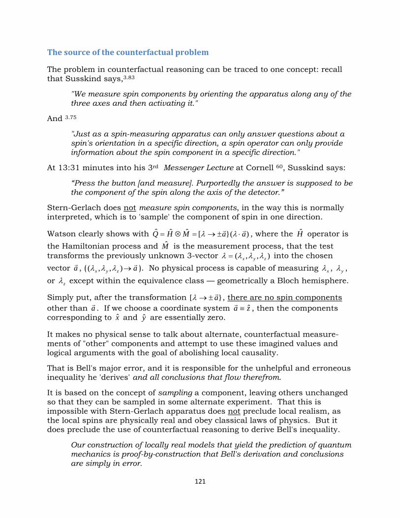
The source of the counterfactual problem The problem in counterfactual reasoning can be traced to one concept: recall that Susskind says,3.83

"We measure spin components by orienting the apparatus along any of the three axes and then activating it."

And 3.75

"Just as a spin-measuring apparatus can only answer questions about a spin's orientation in a specific direction, a spin operator can only provide information about the spin component in a specific direction."

At 13:31 minutes into his 3rd Messenger Lecture at Cornell 60, Susskind says:

“Press the button [and measure]. Purportedly the answer is supposed to be the component of the spin along the axis of the detector.”

Stern-Gerlach does not measure spin components, in the way this is normally interpreted, which is to 'sample' the component of spin in one direction.

Watson clearly shows with )([ˆˆˆ aaMHQ ⋅±→=⊗= λλ , where the H operator is

the Hamiltonian process and M is the measurement process, that the test transforms the previously unknown 3-vector ),,( zyx λλλλ = into the chosen vector a , ( azyx

→),,( λλλ ). No physical process is capable of measuring xλ , yλ ,

or zλ except within the equivalence class — geometrically a Bloch hemisphere. Simply put, after the transformation [ a±→λ , there are no spin components other than a . If we choose a coordinate system za ˆ≡

, then the components corresponding to x and y are essentially zero. It makes no physical sense to talk about alternate, counterfactual measure-ments of "other" components and attempt to use these imagined values and logical arguments with the goal of abolishing local causality.

That is Bell's major error, and it is responsible for the unhelpful and erroneous inequality he 'derives' and all conclusions that flow therefrom. It is based on the concept of sampling a component, leaving others unchanged so that they can be sampled in some alternate experiment. That this is impossible with Stern-Gerlach apparatus does not preclude local realism, as the local spins are physically real and obey classical laws of physics. But it does preclude the use of counterfactual reasoning to derive Bell's inequality.

Our construction of locally real models that yield the prediction of quantum mechanics is proof-by-construction that Bell's derivation and conclusions are simply in error.

121

Entanglement and Steering

A ubiquitous theme in physics is 71:

"…in 1964, Bell showed that the laws of quantum mechanics are inconsist-ent with the description of our world based on local elements of reality."

In discussing Bell's theorem we noted that Peres states:

"Bell’s paper is not about quantum mechanics… It is a general proof [of a limit on correlations ]… if one just assumes the validity of local causes."

Though Bell defines ‘local causality’ rather simply, I translate the sense of the above as believing the magnetic moment is somewhat of a bull-in-a-china-shop, smashing its way through all impediments, taking no heed of local surround-ings. But it is not like that in reality. Delicate magnetic moments, however currently aligned, can be tossed like a boat on the ocean, and Stern-Gerlach brews up a perfect local storm.

The idea of spin as impervious to local surroundings is embodied in Bell's naïve model in which λ , the initial spin, is described in a way that, independently of the travails it traverses, can be 'sampled', component-by-component, at the end of its voyage, and this can be used with counterfactual reasoning ( imagined, but not tested ) to conclude that local reality is incapable of describing what actually happens. The use of imagined components to reason physically leads to other imaginary phenomena such as entanglement — the idea that launched 1000 papers. For a perfect example of this watch Susskind's "Entanglement—the hooks that hold space together." In this, his third Messenger Lecture at Cornell 60 Susskind says:

"We have a spin – a little bitty physical system – attached to an electron – and it has an arrow associated with it – in other words a vector – it's something you can measure, and when you measure it you measure its components: it's x-component, its y-component and its z-component. … To measure it, you bring the apparatus up to the spin… press the button and you get an answer.

Purportedly the answer is supposed to be the component of the spin along the axis of the detector. You always get, in quantum mechanics, either + or -1. No intermediate answer, nothing in between. 1± . This is a little bit peculiar, that the component of a vector in an arbitrary direction should be +1 or -1, but we understand this, this is quantum mechanics. This is the weirdness of quantum mechanics.”

I don't think Susskind means "we understand this". I think he means "we're accustomed to this, and we accept it." He goes on in this talk to explain that

122

"Space can't hold itself together: entanglement equals the hooks that hold space together."

The belief that local causality cannot account for "quantum correlations" led to the idea that the remote particles are "entangled" in some distance-independ-ent manner. What, in classical physics, would have been attributed to simple ‘conservation of momentum’ was sabotaged by Bell, when he ‘proved’ classical mechanisms cannot produce the ‘quantum correlations’. If particles are not conserving angular momentum , then they must be ‘entangled’ in some other way. In this regard, Hirsch et al. state that 72:

“Performing local measurement on separated entangled particles can lead to nonlocal correlations, as witnessed by the violation of a Bell inequality… However, 50 years after the discovery of Bell’s theorem, we still do not fully understand the relation between entanglement and nonlocality…”

‘Entangled’ particles “as witnessed by violation of a Bell inequality.” Is there anything other than the violation of a Bell inequality that points to entangle-ment? Anything at all? No, there is not!

Despite that measurements ‘confirm’ quantum correlations, many agree with Aspect, that entanglement is "difficult to swallow". In discussing the correlated states of identical particles as "strongly … entangled", Killoran, et al.73 state:

“..the notion of entanglement for identical particles is troublesome… [ due to indistinguishability ] . Many authors share the viewpoint that such entanglement is a mathematical artifact, and not fully legitimate…"

Even Susskind states 3.231:

"Of all the counterintuitive ideas quantum mechanics forces on us, entanglement may be the hardest one to accept."

A variant of the idea of entanglement is that of EPR-'steering', described as 74 :

Two parties, Alice and Bob, share an entangled state ⟩ABψ| . By measuring her subsystem, Alice can remotely change ( i.e., steer ) the state of Bob’s subsystem in such a way that would be impossible if their systems were only classically correlated."

Thus, whether non-locality, entanglement, or steering, faith in Bell’s claim that observed correlations cannot arise from local realism leads to unreal notions of superluminal effects acting over arbitrary distances. How does this differ from pure magic? I don't think one can say.

123

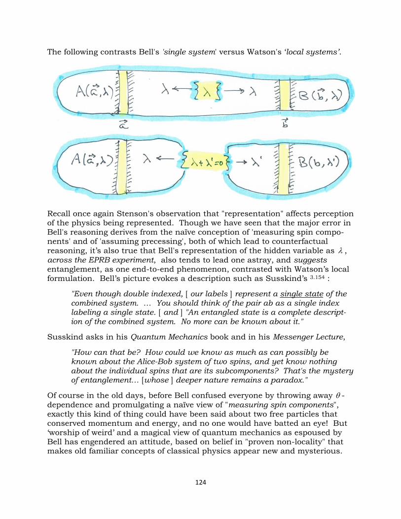
The following contrasts Bell's 'single system' versus Watson's ‘local systems’.

Recall once again Stenson's observation that "representation" affects perception of the physics being represented. Though we have seen that the major error in Bell's reasoning derives from the naïve conception of 'measuring spin compo-nents' and of 'assuming precessing', both of which lead to counterfactual reasoning, it’s also true that Bell's representation of the hidden variable as λ , across the EPRB experiment, also tends to lead one astray, and suggests entanglement, as one end-to-end phenomenon, contrasted with Watson’s local formulation. Bell’s picture evokes a description such as Susskind’s 3.154 :

"Even though double indexed, [ our labels ] represent a single state of the combined system. … You should think of the pair ab as a single index labeling a single state. [ and ] "An entangled state is a complete descript-ion of the combined system. No more can be known about it."

Susskind asks in his Quantum Mechanics book and in his Messenger Lecture,

"How can that be? How could we know as much as can possibly be known about the Alice-Bob system of two spins, and yet know nothing about the individual spins that are its subcomponents? That's the mystery of entanglement… [whose ] deeper nature remains a paradox."

Of course in the old days, before Bell confused everyone by throwing away θ -dependence and promulgating a naïve view of "measuring spin components", exactly this kind of thing could have been said about two free particles that conserved momentum and energy, and no one would have batted an eye! But ‘worship of weird’ and a magical view of quantum mechanics as espoused by Bell has engendered an attitude, based on belief in "proven non-locality" that makes old familiar concepts of classical physics appear new and mysterious.

124

"So it seems that in quantum mechanics, we can know everything about a composite system – everything there is to know, anyway – and still know nothing about its constituent parts. This is the true weirdness of entanglement, that so disturbed Einstein." 3.175

Of course if we rephrase this:

So it seems that in classical mechanics, we can know everything about a composite system – a system that conserves momentum – and still know nothing about [ the individual momentum of ] its constituent parts. Even Newton understood this.

But of course Newton was not confused by ‘collapse of the wave function’, or ‘deleted degrees of freedom [θ ]’, ‘entanglement’, and other misleading concepts that Bell helped push on the world. And the duality of 'wave and particle', combined with the formalism of quantum mechanics, in some sense obscures natural phenomena that were quite clear to Newton. Complexity masks the transparency of the system. It takes time to be comfortable with 3.198

"When the density matrix corresponds to a single state, it is a projection operator that projects onto that state. In this case we say that the state is pure… [ and ] represents the maximum amount of knowledge that Bob can have of a quantum system."

By the time a student has been indoctrinated with quantum worship and has absorbed enough math to use density matrices and projection operators, he has also absorbed enough of Bell's 50-year-old ideas of non-locality, steering, entanglement, and collapse of the wave function to be almost beyond the possibility of actually understanding quantum phenomena. Those confused ideas have so distorted today's physics that Aephraim Steinberg says 70

"Too many physicists have fallen prey to the reassuring but nihilistic thesis that since so many before us have failed, we would be wasting our time to seek any deeper understanding of quantum theory ( than is contained in our beautiful equations. )

Susskind continues 3.213:

"Entanglement is the quantum mechanical generalization of correlation.… It indicates that Alice can learn something about Bob's half of the system by measuring her own."

Of course we have explained this in terms of the local equivalence classes defined by Alice or Bob's measurement, with no need for entanglement or for collapse of the wave function, but many physicists will not appreciate this. It is too far removed from their beliefs about the primacy of quantum mechanics.

125

Brief summary To briefly summarize the key points of the quantum mechanics situation: 1. Correspondence between measurement and operator is fundamental to QM. 2. Operators are constructed to represent components of spin. 3. Spin components are measured by orienting the apparatus. Our theory of quantum events, with the Energy-Exchange theorem and [ a±→λ operation implies alignment of initial spin, which conflicts with #3, that is, we do not measure spin components in a given direction. The entire electron spin is transformed to point in a specific direction:

There are no other components! But counterfactual reasoning is based on the belief that we are measuring the ‘components’ of spin, and belief that a different measurement would measure a different 'component'. That is the basis of Bell's error in deriving his inequality. And the basis for physicists’ current belief that local realism does not exist and superluminal entanglement does.

So the counterfactual fallacy is based on a naïve interpretation of measurement as sampling a component of spin, based in turn on classical knowledge of spin, which is a 3-space phenomenon, and on a 1D net that passes two directions of spin. Because physicists believe they’re measuring a 'component' of spin, instead of spin, per se, they reasonably assume that other components exist and could have been measured. This is the basis of counterfactual reasoning. We have shown that both the magnetic moment’s configuration energy and the deflection energy of the particle are coupled to a common parameter, θ , and hence θεθε dddd 10 −= and a finite amount of precession energy is dissipated as deflection energy and entropy increases. Via the Hamiltonian for changing fields the net result is that the aligned spin has only one direction, the direction produced by the experimental apparatus. No other test of 'another spin component' would produce anything different, or relevant.

When this is understood, no more worry!

I conjecture that the wave function of quantum mechanics is a tensor product of the linear momentum-based wave function ( in which a real circulating field is induced by real linear momentum ) and the angular momentum- or spin-wave function, in which the real spin is transformed and only the 'equivalence class' remains [i.e., incomplete information],

yielding both epistemic and ontic aspects of the wave function.

This may help explain why this basic question is still unanswered.

126

Conclusion: the Quantum Theory of Events

We began with a 35-year-old analysis (The Automatic Theory of Physics) of how robots could be designed, programmed, or 'taught’ to do physics. This led us to three problems: 1) generating numbers, 2) manipulating numbers, and 3) assigning numbers to physical entities. The first two are easily solved struct-urally, by implementing logic structures in material form. The assignment is performed algorithmically by implementing clustering algorithms followed by pattern recognition algorithms with entropy-based measures of 'best fit'.

As it turns out, myriads of numbers can be produced by any robot interacting (experimenting) with its environment. Some numbers do not change and some cycle endlessly. It was therefore found to be useful, FAPP 'necessary', to define classes of behaviors, and one of the most useful classes was found to be the 'event', defined as an initial state (or set of numbers) followed by transition to a final state (a new set of numbers.) Following such procedures it was found that "rules of behavior" could be generated and "theories" of physics invented. We also developed means to determine the "best" theories, again based on entropy measures. It was later found, by Schmidt and Lipson53, that the robot could control the type of law by choosing what variables to provide to the algorithms.

"… If we only provide position coordinates, the algorithm is forced to converge on a manifold equation of the system’s state space. If we provide velocities, the algorithm is biased to find energy laws. If we additionally supply accelerations, the algorithm is biased to define force identities and equations of motion."

The result of this exercise yielded both classical physics and a Hilbert space representation of discrete states or 'features' of local physical entities.

Recently, in analyzing the Stern-Gerlach experiment, it became obvious that two different energy modes are linked through common variable, θ , in this case the "angle of precession". This led to the 'energy-exchange theorem'

θε

θε

dd

dd 10 −= , 2- 132

and the realization that the initial spin λ , entering the apparatus, is trans-formed to the control setting a and then it is measured. Watson, independ-ently, analyzed such fundamental transformations formally, using the Q-operator MHQ ˆˆˆ ⊗= where [ˆ aH

±→= λ and )(ˆ aM ⋅= λ . He did so in the

context of Bell's theorem, an inequality derived 50 years ago and used as the basis of a claim that local causal models are impossible to construct, since

babAaAd⋅−≠− ∫ ),(),()( λλλρλ 2- 133

127

while the quantum mechanics of the corresponding singlet state yields

baba⋅−=⟩⋅⋅⟨ ξσσξ |ˆˆ| 2- 134

The consequence has been a half-century of 'magical thinking' with superlum-inal effects and 'entanglement' spreading over space-time. And yet no one has found the smoking gun, the ‘hole’ or broken link in Bell's chain of logic. Watson has criticized Bell's use the same λ for ⟩⟨ab and ⟩⟨ac since all Stern-Gerlach tests are of paired spins and are not repeatable. Thus the λ for a tested against b

and the λ for a tested against c cannot be the same λ .

Many physicists argue against this, claiming that Bell is not analyzing experiments, but is simply stating what kinds of math models can be built. I think that is a difficult argument to make, and not wholly consistent. Peres states 15.162 that Bell's theorem is not about quantum mechanics (per se) but

"Applies to any physical system with dichotomic variables, where values are arbitrarily called 1+ and 1− . Its proof involves two distinct observers and some counterfactual reasoning."

[Bell’s logic] "referred to three tests, of which any two, but only two can actually be performed. At least one of the three tests is counterfactual."

The qualification 'dichotomic' is probably unnecessary, it may be proved for N distinct output states, but dichotomic reasoning makes it simpler to analyze. It has been convenient to use Susskind's first two volumes of "The Theoretical Minimum" as a main reference (in addition to Bell's "Speakable…") and one particularly useful section involves "constructing the quantum mechanical representation of the dichotomic system." Given that the apparatus always produces 1+ or 1− , observed values can be represented by a 2D Hilbert vector

=⟩+

01

| and

=⟩−

10

| 2- 135

and the (Hermitian) linear operator that fulfills the quantum 'formula'

⟩±=⟩ ξξσ || . 2- 136

expressed as a 22× matrix, (the Pauli matrices), where it is clearly stated up front that the goal in this construction is to

"Construct operators to represent the components of spin, zσ , xσ , and yσ " and use these operators 3.83 to

"measure spin components by orienting the apparatus along any of the three axes…"

128

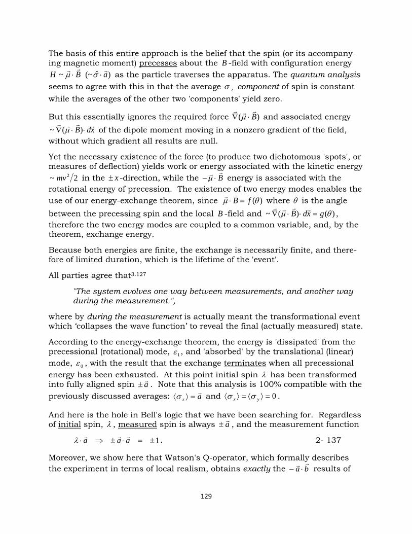
The basis of this entire approach is the belief that the spin (or its accompany-ing magnetic moment) precesses about the B -field with configuration energy

)ˆ(~~ aBH ⋅⋅ σµ as the particle traverses the apparatus. The quantum analysis

seems to agree with this in that the average zσ component of spin is constant while the averages of the other two 'components' yield zero.

But this essentially ignores the required force )( B

⋅∇ µ and associated energy xdB

⋅⋅∇ )(~ µ of the dipole moment moving in a nonzero gradient of the field, without which gradient all results are null. Yet the necessary existence of the force (to produce two dichotomous 'spots', or measures of deflection) yields work or energy associated with the kinetic energy

2~ 2mv in the x± -direction, while the B

⋅− µ energy is associated with the rotational energy of precession. The existence of two energy modes enables the use of our energy-exchange theorem, since )(θµ fB =⋅

where θ is the angle

between the precessing spin and the local B -field and )()(~ θµ gxdB =⋅⋅∇

, therefore the two energy modes are coupled to a common variable, and, by the theorem, exchange energy. Because both energies are finite, the exchange is necessarily finite, and there-fore of limited duration, which is the lifetime of the 'event'. All parties agree that3.127

"The system evolves one way between measurements, and another way during the measurement.",

where by during the measurement is actually meant the transformational event which ‘collapses the wave function’ to reveal the final (actually measured) state.

According to the energy-exchange theorem, the energy is 'dissipated' from the precessional (rotational) mode, 1ε , and 'absorbed' by the translational (linear) mode, 0ε , with the result that the exchange terminates when all precessional energy has been exhausted. At this point initial spin λ has been transformed into fully aligned spin a± . Note that this analysis is 100% compatible with the previously discussed averages: az

=⟩⟨σ and 0=⟩⟨=⟩⟨ yx σσ .

And here is the hole in Bell's logic that we have been searching for. Regardless of initial spin, λ , measured spin is always a± , and the measurement function

1±=⋅±⇒⋅ aaa λ . 2- 137

Moreover, we show here that Watson's Q-operator, which formally describes the experiment in terms of local realism, obtains exactly the ba

⋅− results of

129

quantum mechanics, which Bell insists is impossible for locally real models, and the Q-operator produces the Born probability distribution, as required. But the key aspect of this analysis is the fact that, whatever the initial spin, the final measured spin will be ± the control setting, a . What this means is that there are no other spin components. No other measurement will measure any different result, period. [ 1+ or 1− is what you get, it’s built in. ] Thus counterfactual assumptions of measuring "other" spin components are non-physical, and cannot be used for reasoning about physical models, and most assuredly cannot be used as the basis of the denial of local causality, (and consequent claim of "entanglement".) Finally, one might ask whether John Bell was aware of θ -dependence and of energy-exchange. Yes, he was absolutely aware of the θ -dependence, when he modified the picture as follows:

"Previously, we implicitly assumed for the net force a direction of the field gradient… a force θcosF where θ is the angle between magnetic field (and field gradient) and particle axis. We change to…"

|cos|cosθθF . 2- 138

Thus did Bell intentionally get rid of θ -dependence, and hence the consequent energy-exchange, believing that the moment continues to precess and the spin components continue to have meaning, and thus to support his counterfactual logic. Moreover, Bell states:

"No attempt is made to explain this change in the force law. It is just an ad hoc attempt to account for the observations."

Of course if Bell had attempted to explain the θ -dependence of the results, he may have discovered the energy-exchange theorem 50 years ago and we would have been spared a half century of confusion over local realism! But that is counterfactual speculation. Bell did not prove that ‘all possible ways’ for classical mechanisms to produce quantum results will fail. It is difficult to ‘prove’ issues of hidden entities. That’s why Feynman, 78.154, on believing the reality of ‘never-seen’ quarks, said:

"I am more sure of the conclusions than of any single argument which suggested them to me, for they have an internal consistency which surprises me and exceeds the consistency of my deductive arguments which hinted at their existence."

I believe the internal consistency of the arguments presented herein call for a reconsideration of Bell’s ‘non-locality’.

130

The cup overfloweth

When one thinks that he basically understands the world, with only a few holes left to be filled in, it is difficult to see new phenomena that do not fit the model, or see integration of ideas incompatible with our current understanding – This is alluded to in the classic Zen story of the honored guest visiting a Zen master, hoping to receive wisdom54. At the tea ceremony the master poured for his guest and continued pouring until the tea was overflowing onto the floor. The guest protested and the master replied

"Like this cup, you are too full of your own opinions and speculations. [You must first ] empty your cup."

This classic story could have been written for 21st century physicists. Despite anomalies, ambiguities, unknowns and paradoxes, physicists assume that they understand the basics, notwithstanding Feynman's claim that no one under-stands quantum mechanics. The key phenomenon, discussed at the 1927 Solvay conference and formalized in 1935 as EPR, and the 50-year-old Bell's theorem, have left physicists confused, with many interpretations of quantum mechanics, some seemingly more mathematical than physical. One well-known analysis, by d’Espagnat 59, in "Quantum Theory and Reality" discussed Bell's theorem in terms of three fundamentals: realism, induction, and separability.

By now you know that our model is locally real, contradicting Bell's theorem. This leaves induction and separability as the likely culprits. Bell and most physicists have sacrificed separability, the belief that physically separated particles have no effect on each other. Instead, they are assumed "entangled", with a superluminal causal connection between separated particles. In short, Bell’ists cling to induction, the ability of the mind to draw logical conclusions, and sacrifice realism and separability. This is quite surprising, as no real problem even exists if one merely assumes an error lies in the basic assump-tions. But, for whatever reason, (lack of imagination) physicists would rather give up reality than think they have made a mistake in reasoning. This problem seems to represent a move away from science and toward faith on the part of scientists — faith that they ‘know’ the truth. It’s almost impossible to empty one’s mind of current physics and see things in a new light, but that shouldn’t prevent new interpretations from being offered, as we have done.

If the logic behind our key belief about spin is wrong, it is possible that logic behind other 50 or 100-year old so-called 'facts' may be wrong also.

131

Acknowledgments

I particularly wish to thank Gordon Watson for his invention of the Q-operator formalism and Dick Zacher and Mike Peeler for discussions of Bell's theorem.

Edwin Eugene Klingman

References

1 JS Bell. 1987. Speakable and Unspeakable in Quantum Mechanics, Cambridge 2 L Susskind and Hrabovsky, 2013 The Theoretical Minimum, Basic Books 3 L Susskind and Friedman, 2014 Quantum Mechanics, Basic Books 4 Xiao and Bauer, 2012, "Spin-Wave Excitation in Magnetic Insulators by Spin-

Transfer Torque", Phys Rev Lett 108, 217204 (25 May 2012) 5 JR Stenson, 2005, “Representations for Understanding the Stern-Gerlach

Effect”, thesis BYU 6 RA Howard, 1963, Nuclear Physics, Wadsworth Pub 7 D Hestenes, 1999, New Foundations for Classical Mechanics, Kluwer Pub. 8 LH Ryder, 1996, Quantum Field Theory, 2nd Ed. Cambridge 9 D Griffiths, 2006, Introduction to Quantum Mechanics, 2nd Ed., Pearson 10 W Heisenberg, 1958, Physics and Philosophy, (Harper & Row, New York 11 Brunner, et al. , 2013, "Dimension Witnesses and Quantum State Discrimination"

Phys Rev Lett 110, 150501 (12 April 2013) 12 L Susskind, private communications 13 Brunner, et al., 2010, “Device-Independent Tests of Classical and Quantum

Dimensions”, Phys Rev Lett 105, 230501 (2010) 14 David Bohm, 1951, Quantum Theory, Prentice Hall Pub 15 A Peres, 1995, Quantum Theory: Concepts and Methods, Kluwer Pub. 16 Navascues and Popescu, 2014, “How Energy Conservation Limits Our

Measurements”, Phys Rev Lett, 112, 140502 (11 Apr 14) 17 http://freevideolectures.com/Course/3151/The-Theoretical-Minimum-

Quantum-Mechanics 18 Ivanov and Karlovets, 2013, “Detecting transmission of radiation from a

magnetic moment” , Phys Rev Lett 110, 264801 (28 Jun 2013) 19 R Blatt, 2011, "Spin Flips with a Single Proton" Nature vol. 475 21 Jul 2011 20 Ulmer, et al. Phys Rev Lett 106, 253001 (2011) and 110, 140405 (2013) 21 N Ramsey, 2013, “The Method of successive oscillatory fields”, Physics Today

(Jan 2013) 22 N Ramsey, 1955, “Resonance Transitions Induced by Perturbations at Two…”,

Phys Rev 100, #4 Nov 15, 1955 23 Koller, et al., 2014, "Beyond the Spin Model Approximation for Ramsey

Spectroscopy" Phys Rev Letters 112, 123001 (28 March 2014) 24 M Mansuripur, 2012, "Trouble with the Lorentz Law of Force: Incompatibility

with Special Relativity and Momentum Conservation", Phys Rev Lett 108, 193901 (11 May 2012)

25 D Griffiths, 2013, “Mansuripur’s Paradox”, arXiv:1303.0732 26 DJ Cross, 2012, “Reso;ution of the Mansuripur Paradox”, arXiv:1205.5451 27 Saldanha, 2012, “Comment on “Trouble with the Lorentz…”, arXiv:1205.6858

132



28 J Christian, 2012, Disproof of Bell’s Theorem, Brown-Walker Press. 29 G ‘t Hooft, 2014, “Cellular Automata Basis for Quantum Mechanics”,

arXiv:1405.1548 30 EE Klingman, 2010 The Automatic Theory of Physics, ISBN 978-0-979-17652-4 31 MS Leifer, 2014 "ψ -epistemic models are exponentially bad at explaining the

distinguishability of quantum states", Phys Rev Lett 112, 160404, (25 Apr 14) 32 E Santos, 2004, “Bell’s Theorem and Experiments”, arXiv:0410193 (2004) 33 G Watson, 2014, “Commonsense Local Realism Refutes Bell’s Theorem,”

viXra:1403.0089, 1405.0020 (2014) 34 PG Lewis, et al., 2012, Phys Rev Lett 109, 150404 (2012) 35 C Stuart, 2014, FQXi article, “Why Quantum?” (11 Jun 2014) [link] 36 Einstein, Podolsky, Rosen, 1935, “Can Quantum-Mechanical Description of

Physical Reality Be Considered Complete?”, Physical Review 47, 15 May 1935 37 JQPMaster, 2010, “The Phenomenal Physics of Spin”

[eg.bucknell.edu/~koutslts/Ph332/Text/Chap6_JQPMaster.pdf] 38 EE Klingman, 2010, The Automatic Theory of Physics, ISBN 978-0-979-17652-4 39 Maroney, 2013, “How statistical are quantum states?”, arXiv: 1207.6906 40 Barrett et al. ,2014, “No ψ -epistemic model can fully explain the indistinguish-

ability of quantum states“, Phys Rev Lett 112, 250403 (Jun 2014) 41 Bacciagaluppi & Valentini, 2009,Quantum Theory at the Crossroads, Cambridge 42 Colbeck & Renner, 2012, “Is a System Wave Function in One-to-One Correspond-

ence with Its Elements of Reality?”, Phys Rev Lett 108, 150402 (13 Apr 2012) 43 JS Bell, 1966, "On the problem of hidden variables in Quantum Mechanics"

Reviews of Modern Phys , (1966) 44 EE Klingman, 2013, FQXi essay ‘Gravity and the Nature of Information’ 45 EE Klingman, 2012, FQXi essay ‘The Nature of the Wave Function’ 46 Adare, et al., 2014, Phys Rev Lett 112,222301 (6 Jun 2014) 47 Pusey, Barrett, & Rudolph, 2012, “On the reality of quantum states”

http://arxiv.org/pdf/1111.3328v2.pdf (7 May 2012) 48 PG Lewis, et al, 2012, “Distinct quantum states can be compatible with a single

state of reality”, Phys Rev Lett 109, 150404 (2012) 49 Eisberg and Resnick, 1974, Quantum Physics, John Wiley 50 Reinhard, et al. 2012, "Tuning a Spin Bath through the Quantum-Classical

Transition", Phys Rev Lett 108, 200402 (18 May 2012) 51 Philip Pearle, 2000, “Wave Function Collapse and Conservation Laws”,

arXiv:0004067v2 6 June 2000 52 tabish.freeshell.org/physics/pm 53 Schmidt and Lipson, 2009, ‘Distilling Free-form Natural Laws from Experimental

Data’, Science Vol 324, 3 PR 2009 54 Paul Reps [compiler], 1957: Zen Flesh, Zen Bones, , 1957, Charles E Tuttle, Co. 55 EE Klingman, 2009, The Chromodynamics War, ISBN: 978-0-979-17657-9 56 Wikipedia, 2014, ‘Adiabatic Theorem’, Born & Foch-1928 57 D Bohm, 1942, “A suggested Interpretation of the Quantum Theory in Terms of

“Hidden” Variables, I and II”, Physical Review 85, #2 (15 Jan 1952) 58 M Schlosshauer, Ed., 2011, Elegance and Enigma: The Quantum Interviews,

Heidelberg, Springer. 59 B d’Espagnat, 1979, "Quantum Theory and Reality", Scientific American 60 L Susskind, 2014 Messenger Lecture, (50th after Feynman’s lecture)

http://www.cornell.edu/video/leonard-susskind-3-entanglement

133

http://arxiv.org/pdf/1111.3328v2.pdf

http://www.cornell.edu/video/leonard-susskind-3-entanglement

61 D Hestenes, 2002, Oersted Medal Lecture 2002 62 JJ Sakurai, 1994 , Modern Quantum Theory, Addison-Wesley Pub, 1994 63 Nassar and Miret-Artes, 2013, "Dividing line between Quantum and Classical

…", Phys Rev Lett 111, 150401 (11 October 2013) 64 Kochan et al., 2014, "Spin Relaxation Mechanism in Graphene…", Phys Rev Lett

112, 116602 (21 March 2014) 65 Golter and Wang, 2014, "Optically Driven Rabi Oscillation… of Single Electron

Spins in Diamond", Phys Rev Lett 112, 116403 (21 March 2014) 66 A Kalev, 2013, “Choice of Measurement as the Signal", Phys Rev Lett 110,

260502 (28 June 2013) 67 T Grover, 2014, "Entanglement Monotonicity…", Phys Rev Lett 112, 151601 (18

April 2014) 68 CD Cothran, et al., 2009, “Observation of a Helical Self-Organized State…”, Phys

Rev Lett, 103, 215002 (20 Nov 2009) 69 Aharonov et al.,2012, “Can a Future Choice Affect a Past-Measurement's

Outcome?" , arXiv:1206.6224 (27 Jun 2012) 70 A Steinberg, 2003, "Speakable and Unspeakable, Past and Future", arXiv:

0302003, (31 Jan 2003) 71 Asadian, Brukner, Rabl, 2014, "Probing Macroscopic Realism…" Phys Rev Lett

112, 190402 (16 May 2014) 72 Hirsch et al., 2013, “Genuine Hidden Quantum Nonlocality”, Phys Rev Lett

111,160402 (18 Oct 2013) 73 Killoran, Cramer, and Plenio, 2014, "Extracting Entanglement from identical

particles", Phys Rev Lett, 112, 150501, (18 April 2014) 74 Skrzypcyzyk, Navascues, and Cavalcanti, 2014, "Quantifying EPR Steering",

Phys Rev Lett 112, 180404 (9 May 2014) 75 Busch and Loveridge, 2011, "Positive Measurements Obeying Momentum

Conservation", Phys Rev Lett 106, 110406 (18 March 2011) 76 J Ozawa, 1984, J. Math. Phy. (NY) 25, 79 (1984) 77 Barrett, et al., 2002, “Quantum non-locality, Bell inequalities, and the memory

loophole”, arXiv 0205016v3 (5 Oct 2002) 78 A Pickering, 1984, Constructing Quarks, Edinburgh Univ. Press 79 CA Fuchs, 2010, “QBism, the Perimeter of Quantum Bayesianism”,

arXiv:1003.5209 (2010) 80 EE Klingman, 2014, FQXi esay: The Thermodynamics of Freedom 81 M Feeley, 2013, FQXi essay: “Without Cause”, 2013 82 ET Jaynes, 2003, Probability Theory: the Logic of Science, Cambridge Press 83 G Watson, 2014, Private communications 84 G Watson, 2014, “Bell’s 1964:(15) is False”, viXra:1406.0027 (2014)

134

Documents

Quantum Spin and Local Reality - viXravixra.org/pdf/1408.0005v2.pdfAlmost a century ago Stern-Gerlach laid important foundations for quantum mechanics. Based on these, Bell formulated