Embed Size (px)
Citation preview
Quantum random walk search on satisfiability problems
Stephan Hoyer
Swarthmore CollegeDepartment of Physics and Astronomy
April 1, 2008
Adviser: David A. MeyerDepartment of MathematicsUniversity of California San Diego

Abstract
Using numerical simulation, we measured the performance of several poten-tial quantum algorithms, based on quantum random walks, to solve Booleansatisfiability (SAT) problems. We develop the fundamentals of quantum com-puting and the theory of classical algorithms to indicate how these algorithmscould be implemented. We also discuss the development of quantum randomwalks and the principles that go into creating them, presenting existing workon search algorithms using coined discrete-time quantum random walks. Al-though our quantum algorithms do not solve SAT problems faster than may bedone classically, as a step toward that objective, we present the first exampleof a quantum walk on a directed graph that has a significant increase in speedover the analogous classical walk.

Contents
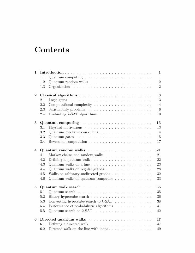
1 Introduction . . . . . . . . . . . . . . . . . . . . . . . . . . . . . . 11.1 Quantum computing . . . . . . . . . . . . . . . . . . . . . . . 11.2 Quantum random walks . . . . . . . . . . . . . . . . . . . . . 21.3 Organization . . . . . . . . . . . . . . . . . . . . . . . . . . . 2
2 Classical algorithms . . . . . . . . . . . . . . . . . . . . . . . . . 32.1 Logic gates . . . . . . . . . . . . . . . . . . . . . . . . . . . . 32.2 Computational complexity . . . . . . . . . . . . . . . . . . . . 42.3 Satisfiability problems . . . . . . . . . . . . . . . . . . . . . . 62.4 Evaluating k-SAT algorithms . . . . . . . . . . . . . . . . . . 10
3 Quantum computing . . . . . . . . . . . . . . . . . . . . . . . . 133.1 Physical motivations . . . . . . . . . . . . . . . . . . . . . . . 133.2 Quantum mechanics on qubits . . . . . . . . . . . . . . . . . . 143.3 Quantum gates . . . . . . . . . . . . . . . . . . . . . . . . . . 153.4 Reversible computation . . . . . . . . . . . . . . . . . . . . . . 17
4 Quantum random walks . . . . . . . . . . . . . . . . . . . . . . 214.1 Markov chains and random walks . . . . . . . . . . . . . . . . 214.2 Defining a quantum walk . . . . . . . . . . . . . . . . . . . . . 224.3 Quantum walks on a line . . . . . . . . . . . . . . . . . . . . . 234.4 Quantum walks on regular graphs . . . . . . . . . . . . . . . . 284.5 Walks on arbitrary undirected graphs . . . . . . . . . . . . . . 324.6 Quantum walks on quantum computers . . . . . . . . . . . . . 33
5 Quantum walk search . . . . . . . . . . . . . . . . . . . . . . . . 355.1 Quantum search . . . . . . . . . . . . . . . . . . . . . . . . . . 355.2 Binary hypercube search . . . . . . . . . . . . . . . . . . . . . 365.3 Converting hypercube search to k-SAT . . . . . . . . . . . . . 385.4 Performance of probabilistic algorithms . . . . . . . . . . . . . 415.5 Quantum search on 2-SAT . . . . . . . . . . . . . . . . . . . . 42
6 Directed quantum walks . . . . . . . . . . . . . . . . . . . . . . 476.1 Defining a directed walk . . . . . . . . . . . . . . . . . . . . . 476.2 Directed walk on the line with loops . . . . . . . . . . . . . . . 49
6.3 Returning to k-SAT . . . . . . . . . . . . . . . . . . . . . . . . 526.4 General quantum operations . . . . . . . . . . . . . . . . . . . 526.5 Directed quantum walks on any graph . . . . . . . . . . . . . 556.6 Quantum directed walks on 2-SAT . . . . . . . . . . . . . . . 566.7 Conclusions . . . . . . . . . . . . . . . . . . . . . . . . . . . . 57
References . . . . . . . . . . . . . . . . . . . . . . . . . . . . . . . . . 61

Chapter 1
Introduction
1.1 Quantum computing
Quantum computing offers a physically based model for computation that maybe fundamentally more powerful than the computational model used for com-puters today. Originally suggested by theoretical physicists Richard Feynmanand David Deutsch in the 1980’s, quantum computing remained little morethan a curiosity until Peter Shor’s discovery of a polynomial time integer fac-torization algorithm in 1994 and Lov Grover’s subsequent development of aquantum search algorithm in 1996 [13, 12, 29, 14]. The discovery of thesepractical algorithms launched a flurry of interest which continues to this day.Fundamental theoretical difficulties with quantum noise and error correctionhave been resolved, meaning that in principle, these computers can be builtand operated efficiently to actually realize their potential [23]. Accordingly,today the race is on to build scalable quantum computers. Many scientistsnow believe that almost inevitably such machines will be built, however manyyears that may be down the line.
But even when they are finally built, the hardware for quantum computerswill require software, and as yet this software—algorithms to run on quantumcomputers—remains very limited. Shor’s factoring algorithm and Grover’ssearch algorithm remain the foundations of the two main families of usefulquantum algorithms. There is the additional likelihood of efficiently simu-lating real world quantum mechanical systems for chemistry, but these algo-rithms remain remarkably limited compared to the set of algorithms still mostefficiently run on classical computers. Finding new and innovative quantumalgorithms is hard, because classical intuitions no longer hold. Regardless, thistask is important both to justify the expense and effort that will be required tobuild such machines, and also because the realm of quantum algorithms stillseems to hold untapped potential. One such family of algorithms of recentinterest and potential are those based on so-called quantum random walks [5].
2 Chapter 1. Introduction
1.2 Quantum random walks
The classical random walk is one of the most basic concepts of probability.When formulated with a finite number of states, it consists of randomly choos-ing paths between vertices on a graph, and many randomized algorithms forcomputing are such walks. These randomized algorithms are significant be-cause they are often some of the simplest and fastest known ways to solve hardproblems [22]. Important applications include solving a variety of graph theoryproblems, the fastest known tests of primality, and solving boolean satisfiabil-ity problems. Similarly, random walks and Brownian motion are at the coreof statistical mechanics. Random walks have a clear appeal to both physicistsand computer scientists: they are a powerful tool for both describing physicalphenomena and writing algorithms.
Not surprisingly then, the quantum random walk can be developed fromboth physical and computational directions as well. A quantum walk is definedby the quantum mechanical movement of a particle on a graph such that ifits position were measured continuously, the probability distribution wouldbe a classical random walk. These walks also arise as the simplest versions ofquantum cellular automata, and as it turns out, include a discrete version of theDirac equation of relativistic quantum mechanics [19]. These walks have verydifferent properties from classical walks, as they do not converge to limitingdistributions and potentially spread much faster. As with classical walks onclassical computers, quantum walks could be run directly and efficiently onquantum computers.
Our focus is on the algorithmic applications of discrete time quantumwalks. The frequent faster spreading of quantum walks offers some possi-bility to improve the performance of randomized algorithms by running themas quantum walks instead, but doing so with most randomized algorithmsof interest is difficult as there is no direct translation. We consider severaltechniques to do so using the problem of boolean satisfiability (SAT), of cen-tral interest to theoretical computer science, as a conceptual and quantitativeframework to guide our investigations.
1.3 Organization
We begin discussing the classical theory of algorithms as necessary to under-stand both quantum computing in general and the specific problems we areattempting to solve (Chapter 2). We follow with an introduction to the founda-tions of quantum computing (Chapter 3), and introduce the notion and powerof the quantum random walk (Chapter 4). Specific techniques for speedingup satisfiability problems in the form of quantum walk search are explored inChapters 5 and 6.

Chapter 2
Classical algorithms
This chapter lays the groundwork in computer science necessary to understandquantum computing and the challenges in creating quantum algorithms. Wereview logic gates and computational complexity, and then consider in depththe problem of boolean satisfiability for which we hope to find a quantumalgorithm.
2.1 Logic gates
There are a number of equivalent theoretical models for classical computation,but the fundamental model used by all modern computers is that of bits andlogic gates. The fundamental unit of information is a bit, either 1 or 0. Largerblocks of information are represented by combinations of bits, so bits strungtogether encode individual letters, documents, pictures, sound and so forth.Thus data is represented by a string of n bits denoted 0, 1n.
Each operation on a classical computer then may be considered as mapping0, 1n → 0, 1m for some n and m. These operations are called logic gates.Classical computers rely on the principle that any logic gate can be constructedfrom repetition of a small finite set of logic gates that only act on a few bits,so all computation can be done with binary logic. Furthermore, each of theseoperation can be built from a small set of fundamental one or two bit operationssuch as not, and and or. One such set is given by the first four entries inTable 2.1. These sets are called universal. Note the inclusion of the fanoutgate. This is often not raised to the level of a logic gate, as in a digital circuitduplicating bits is as simple as attaching another wire. But the same sort ofwiring does not work in a quantum circuit, so it is best to make all operationsexplicit. It is an easy exercise to show that nand (not and) with appropriatedummy inputs can simulate each of the first three gates, so as it turns out,merely the operations nand and fanout form a universal gate set.

4 Chapter 2. Classical algorithms
Gate Input → Outputand (a, b)→ abxor (a, b)→ a⊕ bnot a→ a⊕ 1
fanout a→ (a, a)nand (a, b)→ ab⊕ 1
Table 2.1: Classical logic gates defined by their action on a, b ∈ 0, 1. ⊕denotes addition modulo 2.
2.2 Computational complexity
Stating the computational resources that an algorithm requires is more so-phisticated than it may seem. It is easy to use a stopwatch to see how fasta program runs, but such a metric is not very useful. It is dependent on theparticular hardware on which the program is run, and the computers of to-day vary widely in speed, and are all overwhelmingly faster than those useddecades ago. Instead, we could count the number of fundamental operationsrequired, but this measure is still not universally meaningful because the samealgorithm may tackle problems of widely varying difficulty and which problemsare good benchmarks may change over time. Imagine we have a route-findingalgorithm that takes a map and destinations as input and outputs an optimaldriving plan. The measure of how long it takes to find a route from Philadel-phia to New York might be a useful basis for comparison, but this is not whywe wrote the algorithm in the first place. We want to know roughly how longthe algorithm takes to find optimal routes based upon the map provided andthe destinations. In particular, we are interested in how the time requirementsfor calculation scale in terms of quantitative measures like the number of junc-tions and the distance between destinations. Finally, we usually do not carehow hard the easy cases are. If the same algorithm will be solving problemsat vastly different scales of difficulty at comparable frequencies, it is the hardproblems that determine the computational requirements.
Accordingly, computer scientists quantify the scaling of an algorithm bydescribing how characteristics like the time or memory space required scaleas a function of input size n as it grows asymptotically large. A resourcerequirement given by f(n) is described asO(g(n)) if f(n) ≤ c·g(n) for all inputsas n→∞ with some constant c. Likewise it is described as Ω(g(n)) if f(n) ≥ d·g(n) for all input as n→∞ with some constant d, and Θ(g(n)) if both O(g(n))and Ω(g(n)). Accordingly O(g(n)) gives an upper bound on the requirementin the worst case of input parameters of size n, whereas Ω(g(n)) gives a lowerbound in the best case. This notation gives a useful definition of speed andspace requirements for algorithms independent of physical implementations.The difference in speed for an algorithm proceeding at some simple multipleof the speed of another is usually not interesting, because faster computerswith identical design scale in performance in the same way. Since again the
2.2. Computational complexity 5
hardest cases are usually of the most interest, the notation using O(f(n)),labeled “big O” notation, is the most common basis for comparison betweenalgorithms.
Problems are divided into computational complexity classes generally bythe time requirements of their best possible algorithms using big O notation.The two main complexity classes used to classify the difficulty of problemsare P and NP. These classify problems known as decision problems, thosewith only yes or no answers. This may seem overly restrictive, but nearly anyproblem can be rewritten as a decision problem. For instance, we could restateour route optimal route finding algorithm as the question of whether or notthere is a route from A to B of less than X total miles. P stands for the classof such problems that can be solved in deterministic polynomial time, that isin time O(poly(n)) where poly(n) is any polynomial of n. NP stands for theclass of problems to which proposed solutions can be verified in polynomialtime. A proposed solution gives a full description of a potential answer, so wecan quickly check the answer to the decision problem. For instance, given aroute between A and B, we can quickly check if it is less than X miles. Anyproblem in P is in the class NP as well, since we can merely run the entirealgorithm to test any proposed solution. Problems in NP but not P are usuallyconsidered to run in exponential time, even though strictly there exist rarelyencountered functions which are asymptotically larger than any polynomialbut smaller than any exponential.
More colloquially, P can be considered as the class of “easy” problemswhereas NP in general includes the class of hard problems as well. This break-down makes sense because of the observation usually referred to as Moore’slaw, that the power of computers grows exponentially over time, which hasremarkably held true for the most part since when Moore first stated it overfour decades ago. Since t→∞, exp(t) > poly(t) for all exponential and poly-nomial functions, so eventually a polynomial requirement will always be lessthan an exponential one. Furthermore, an exponential increase in computa-tional resources means that all problems that can be solved in polynomial timecan eventually be done easily for nearly any input size, whereas problems thatare exponentially hard will always remain hard.
Another subset of NP, termed NP-complete, is the set of all problems towhich a solution can efficiently be used to solve any other problem in NP.Similar to the distinction between P and NP, “efficient” in a technical sensemeans that a solution to the original problem would only need to be repeatedsome at most some polynomial (sub-exponential) number of times to createa mapping to the other problem. Since any NP-complete can be efficientlymapped onto other hard problems, in some sense this is class of “hardest”problems.
One of the most significant open questions in computer science and mathe-matics is whether P is equal to NP. To show P=NP, it would suffice to find oneexample of an NP-complete problem that is also in P, as this problem could beadapted to every other problem in NP. Such a result would have revolutionary
6 Chapter 2. Classical algorithms
implications for computer science, as then nearly all hard problems could besolved with relative ease. Accordingly, nearly all complexity theorists believethat P 6=NP.
The power of quantum computers comes because there are a number ofquantum algorithms fundamentally faster than the best known classical al-gorithms, in the sense of big O asymptotic notation. There are problemsthat computer scientists believe cannot be solved classically in sub-exponentialtime, but can be solved in polynomial time on a quantum computer, themost notable example of these problems being integer factorization. The bestclassical algorithms take exponential time to factor large, but on a quantumcomputer, using Shor’s algorithm, integer factorization can be done in polyno-mial time [29]. But importantly, integer factorization is not NP-complete. Ifso, quantum computers could solve nearly any computational problem easily.Quantum information theorists do not expect to find any such problems either,as this would imply in some sense a lack of bounds in the computational powerof physical systems [1]. Quantum computers are good, but not that good.
2.3 Satisfiability problems
The problem of boolean satisfiability (SAT) is one of the archetypal NP-complete problems. A satisfiability formula is given by any logic gate orcombination of gates that takes n bits to 1 bit. Such a formula is said tobe satisfiable if there exists a truth assignment—a set of bit values assignedto each variable—such that the entire statement evaluates to 1. The SATproblem is then the question of whether or not a given satisfiability statementis satisfiable. Clearly this is a decision problem, and since it can be checkedin polynomial time if a proposed truth assignment evaluates to 1 or 0, thisproblem is in NP. It should not be surprising that SAT is NP-complete, sinceas we already noted logic gates form the fundamental building blocks of mod-ern computers. Thus the statement that SAT is NP-complete is equivalent tonoting that any hard problem can be run with roughly equivalent efficiencyon the hardware of a modern computer.
As it turns out, there is far more flexibility in SAT formulas than is requiredfor NP-completeness. A useful subset of SAT formulas are those that can bewritten in k conjunctive normal form (k-CNF). A formula in k-CNF consistsof literals defined as one of n variables or their negation, of which groups of kare combined by or to form clauses, with m clauses combined by and. As aconcrete example, consider the following formula:
k literals per clause︷ ︸︸ ︷(a or ¬b or c) and (¬a or b or d) and (¬a or a or ¬c)︸ ︷︷ ︸
m clauses with literals chosen from n variables (a, b, c, d, . . .) and their negations (¬a = not a)
.
The problem of k-satisfiability (k-SAT) consists of all SAT formulas in k-CNF.As it turns out, k-SAT is also NP-complete for k ≥ 3. Since 3-SAT is NP-

2.3. Satisfiability problems 7
000 100
001
010 110
111
101
011
Figure 2.1: The binary hypercube in 3 dimensions. Vertices correspond toeach bit array of length n, and edges connect paths that only differ in one bit.
complete and given by such a prescribed form, it is one of the simplest regularforms of SAT that maintains the full complexity of the problem. Also, sincenumerous other problems have been shown to be NP-complete by noting theirequivalence to 3-SAT, many consider it the canonical NP-complete problem.In fact, the term “SAT” often refers directly to 3-SAT.
Remarkably, even though 3-SAT is NP-complete, 2-SAT with its very sim-ilar form is in P. This means that 2-SAT is actually an easy problem. Wewill prove this by presenting a simple random walk algorithm due to ChristosPapadimitriou [24]:
Guess an initial truth assignment at random.While the SAT formula is unsatisfied:
1. Choose an unsatisfied clause at random.2. Flip the value of the variable associated with a random literalin that clause.
Note that a clause is said to be unsatisfied just as for a complete formula, if itevaluates to 0. We will spend a lot of time analyzing this algorithm becauseit will also be a focus of our interest in random walk search procedures.
Before we present a proof of the speed of this algorithm, there are a fewthings worth observing about it. First, note that we can represent any truthassignment as a position on the binary hypercube in n-dimensions, the n-dimensional space where there are exactly two possible values 0, 1 in eachdimension, as was perhaps alluded to by referring to a string of bits as 0, 1n.A binary hypercube is shown is in Fig. 2.1.
But more specifically to this problem, note that the algorithm given herefor 2-SAT is a random walk algorithm that proceeds along the edges of thisbinary hypercube. In particular, the algorithm proceeds by picking a randomstarting vertex, and then flipping the value of one variable at a time. In fact,this 2-SAT algorithm can be considered as exactly a random walk proceedingalong a directed graph where edges are taken from the set of those appearing

8 Chapter 2. Classical algorithms
<1/2<1/2<1/2
>1/2>1/2>1/2
3210
101
111
110
100
010
011000
001
Solution
Figure 2.2: Reduction of hypercube walk to the line. Vertices are grouped bytheir Hamming distance from a solution, here chosen arbitrarily at 000.
on the binary hypercube, with possibly redundant paths in the case that avariable appears in multiple unsatisfied clauses.
Theorem. If its formula is satisfiable, the 2-SAT algorithm given above ter-minates in O(n2) steps.
Proof. In the worst case scenario that this formula is satisfiable, there is exactlyone satisfying truth assignment, and the initial guess is as far away from thatsolution as possible. We can group truth assignments by how many bits theyhave that are different from the solution. This measure of the number ofdifferent bits is known as the Hamming distance. This grouping by Hammingdistance from x0 = 000 is shown in Fig. 2.2. Since each possible move alongthe hypercube is a change of the value of one bit, each either increments ordecrements the Hamming distance from the solution, so we can consider thisalgorithm as a random walk along the line given by this set of distance valuesas well. If there are n variables, then this walk is along the line [0, n].
At each position along the line, there is at least a 1/2 probability of movingcloser to the solution, because in each unsatisfied clause, there are at most twovariables, at least one of which must have a different value from its value inthe solution. The walk only terminates when it reaches the end of the lineat distance x = 0 from the solution. At the other end, it reflects from theposition of maximum distance x = n to the position x = n− 1 with certainty.
We can write down a recurrence relation for the number of expected stepsEx at position x until the walk terminates in terms of the number of expected
2.3. Satisfiability problems 9
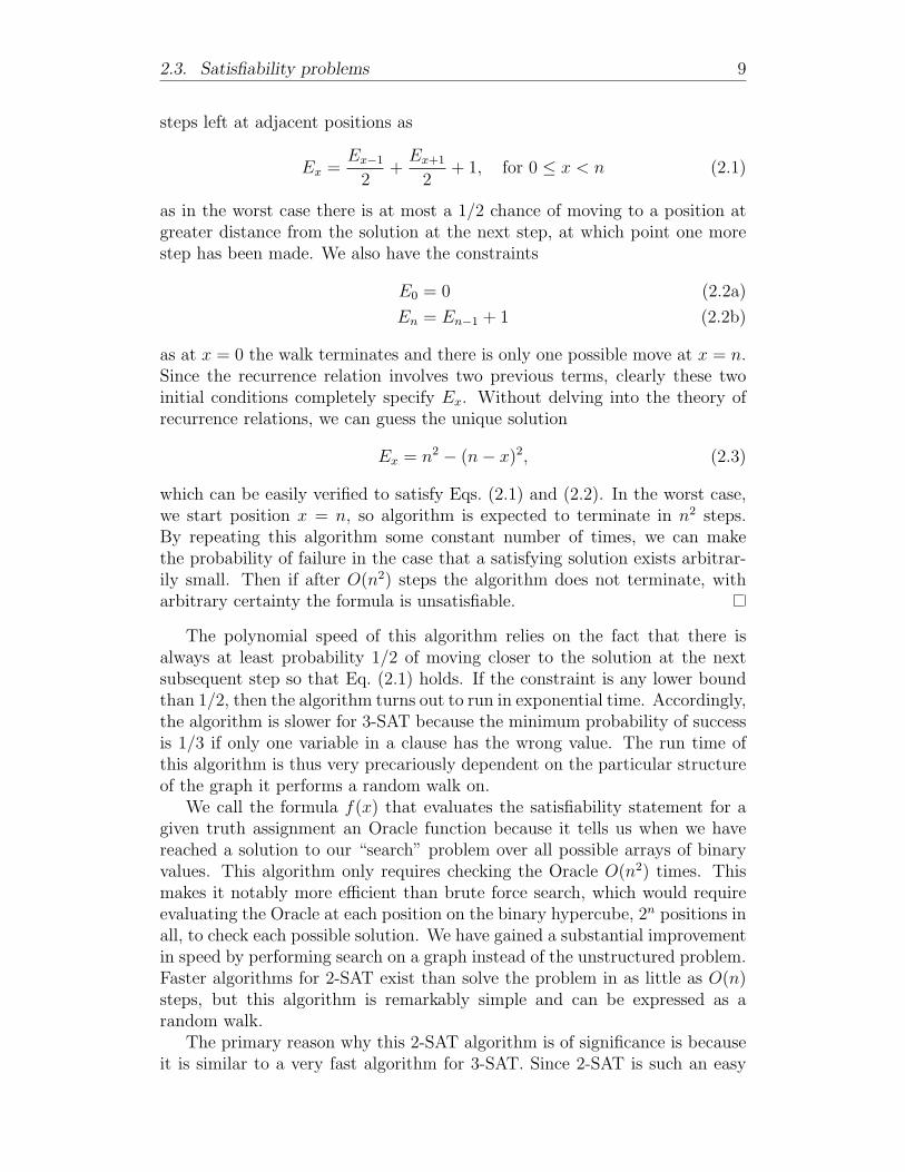
steps left at adjacent positions as
Ex =Ex−1
2+Ex+1
2+ 1, for 0 ≤ x < n (2.1)
as in the worst case there is at most a 1/2 chance of moving to a position atgreater distance from the solution at the next step, at which point one morestep has been made. We also have the constraints
E0 = 0 (2.2a)
En = En−1 + 1 (2.2b)
as at x = 0 the walk terminates and there is only one possible move at x = n.Since the recurrence relation involves two previous terms, clearly these twoinitial conditions completely specify Ex. Without delving into the theory ofrecurrence relations, we can guess the unique solution
Ex = n2 − (n− x)2, (2.3)
which can be easily verified to satisfy Eqs. (2.1) and (2.2). In the worst case,we start position x = n, so algorithm is expected to terminate in n2 steps.By repeating this algorithm some constant number of times, we can makethe probability of failure in the case that a satisfying solution exists arbitrar-ily small. Then if after O(n2) steps the algorithm does not terminate, witharbitrary certainty the formula is unsatisfiable.
The polynomial speed of this algorithm relies on the fact that there isalways at least probability 1/2 of moving closer to the solution at the nextsubsequent step so that Eq. (2.1) holds. If the constraint is any lower boundthan 1/2, then the algorithm turns out to run in exponential time. Accordingly,the algorithm is slower for 3-SAT because the minimum probability of successis 1/3 if only one variable in a clause has the wrong value. The run time ofthis algorithm is thus very precariously dependent on the particular structureof the graph it performs a random walk on.
We call the formula f(x) that evaluates the satisfiability statement for agiven truth assignment an Oracle function because it tells us when we havereached a solution to our “search” problem over all possible arrays of binaryvalues. This algorithm only requires checking the Oracle O(n2) times. Thismakes it notably more efficient than brute force search, which would requireevaluating the Oracle at each position on the binary hypercube, 2n positions inall, to check each possible solution. We have gained a substantial improvementin speed by performing search on a graph instead of the unstructured problem.Faster algorithms for 2-SAT exist than solve the problem in as little as O(n)steps, but this algorithm is remarkably simple and can be expressed as arandom walk.
The primary reason why this 2-SAT algorithm is of significance is becauseit is similar to a very fast algorithm for 3-SAT. Since 2-SAT is such an easy
10 Chapter 2. Classical algorithms
problem, it is generally only of interest because of its connection to 3-SAT.3-SAT is a problem of substantial interest to computer scientists for whichthere have been ongoing efforts to find fast algorithms. As for 2-SAT, thenaive brute-force search of each possible solution runs in 2n steps, but betteralgorithms exist. One of the very best to date is due to Uwe Schoning [26]. Atits core is the same procedure as the 2-SAT algorithm by Papadimitriou, how-ever the loop is only repeated 3n times before the algorithm is run again in itsentirety with a new guess of an initial truth assignment. After some numberof repetitions taking no more than O((4/3)n) steps in total, the algorithm willterminate successfully with arbitrarily high constant probability if a satisfyingtruth assignment exists. Note that the fact that the algorithm repeats is notactually any different from the 2-SAT algorithm, as both only terminate suc-cessfully after some number of steps with some probability. Reaching arbitrarycertainty in either case would require repetition, although in the case of 2-SATit would suffice to merely run continue the same run of the algorithm for longeras well. Although Schoning’s algorithm is no longer remains the very fastestfor 3-SAT, it remains among the best, and many superior algorithms are stillbased off of it.
2.4 Evaluating k-SAT algorithms
Evaluating new algorithms for 2-SAT and 3-SAT by numerical simulation in-stead of analytical techniques requires measuring speed on some set of formulasinstead of establishing some abstract upper bound. But k-SAT problems canvary widely in difficulty, and it is easy to cook up formulas that are either sat-isfiable or unsatisfiable for all truth assignments. The tricky cases are thosethat a priori cannot be categorized as likely satisfiable or unsatisfiable. Thisshould correspond to a set of formulas for which on average it takes a longtime to find a solution, giving some rough estimate of the upper bound.
The simplest way to find k-SAT formulas to test other than taking themdirectly from real world problems would be to generate them uniformly atrandom with n variables and m clauses. If we are interested in measuring theperformance of a k-SAT algorithm at different values of n, then for given n andk, we need to somehow pick the number of clauses m. For randomly generatedformulas, it is clearly far more likely for there to be multiple solutions if m issmall since there is a smaller set of constraints, and as m increases randomlygenerated formulas should be less and less likely to have any solutions at all.This transition between likely satisfiable and likely unsatisfiable formulas canbe considered as sort of numerical phase transition occurring at some criticalratio α = n/m of the number of variables to the number of clauses, and thereis an actually an extensive literature examining these sorts of transitions fromthe perspective of statistical mechanics [9]. Randomly generated formulas atthis phase transition are neither more likely to be satisfiable or not, so theseare the hardest cases. Since some of the best 3-SAT algorithms run slowest
2.4. Evaluating k-SAT algorithms 11
5
4
3
2
1
0
α15105
n
2-SAT
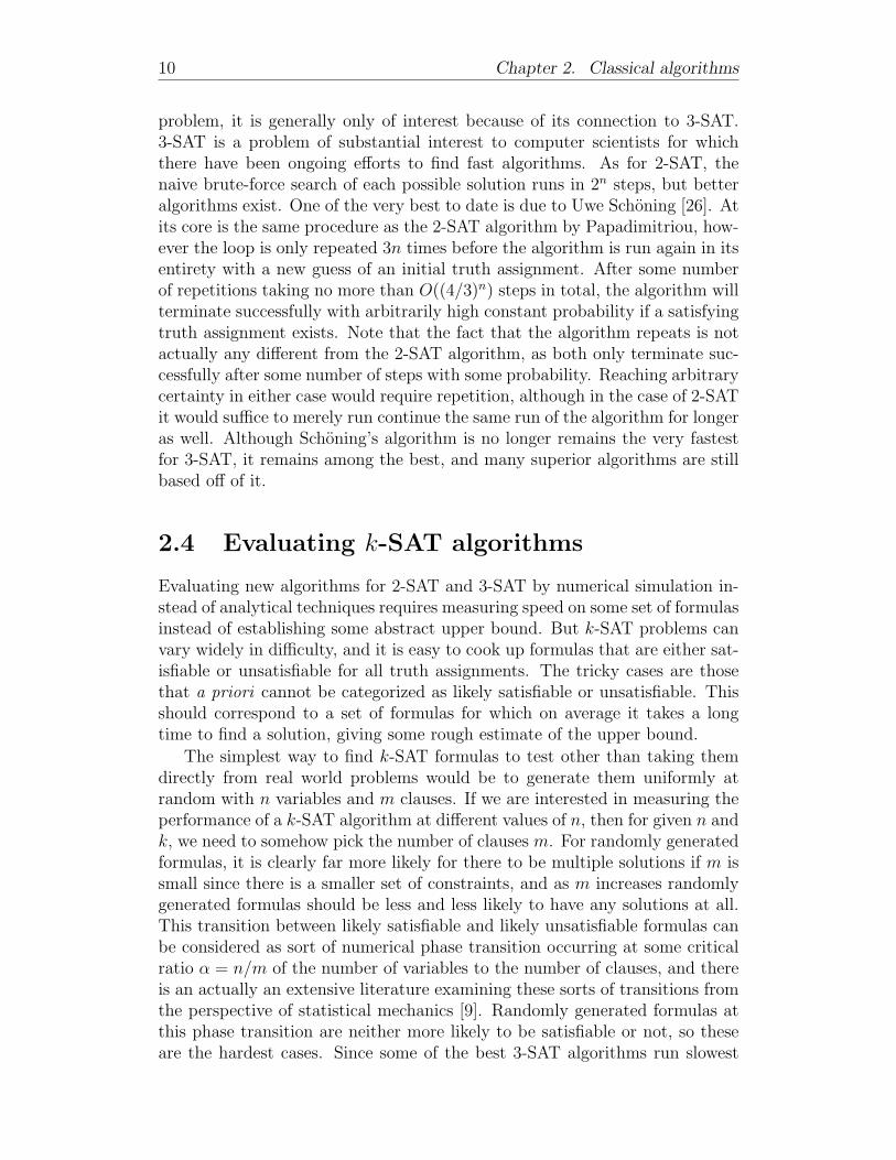
Figure 2.3: Location of phase transition for 2-SAT problems at small n interms of the parameter α = m/n. As n→∞, α = 1 for 2-SAT and α ≈ 4.25for 3-SAT.
on randomly generated formulas at the transition, it makes sense to use thistransition when evaluating the performance of algorithms numerically [15].These algorithmic phase transitions have been studied and classified in thesame sorts of ways as with physical transitions. For example, 3-SAT has afirst-order (discontinuous) transition in terms of the number of clauses m,whereas the transition with 2-SAT is second-order (continuous). It turns outthat in the limit as n → ∞, for 2-SAT this transition is at α = 1 and for3-SAT at about α = 4.25, but the transition moves to this limit relativelyslowly. Accordingly, for use in later numerical trials, we give the location ofthe phase transition for 2-SAT in Fig. 2.3.
Another way to find hard cases is the obvious measure of counting thenumber of solutions. Then k-SAT formulas with only one solution shouldbe the hardest to solve. This is most dramatically true for a random brute-force approach, although in practical instances, we can imagine that multiplesolutions may be clustered structurally, so multiple solutions could be nearlyas hard to find as one solution for a classical random walk or systematic search.There are two obvious ways to generate such statements randomly. One optionis add clauses one by one until a only one solution remains or the formulais unsatisfiable, in which case we backtrack one step. The alternative is torandomly generate formulas at the phase transition and discard them unlessthey have one solution. The distinction is not very important, and accordinglywe will choose the second method, if only because it seems more analogous tothe more general technique.


Chapter 3
Quantum computing
3.1 Physical motivations
The potential of quantum computing is alluded to by the difficulty of simulat-ing quantum systems on a classical computer. For example, consider a systemof 100 particles each with two possible states. If this system were classical,we could write down its state just with 100 zeros or ones. But if this systemwere quantum mechanically, recording its state would involve writing down2100 complex numbers, more numbers to keep track of than the number ofatoms in the visible universe, estimated at roughly 1080. Accordingly there isclearly no way that a classical computer could calculate exactly any sort ofnon-trivial evolution of such a system.
This suggests a natural question leading to quantum computing, originallyby Richard Feynman, of whether such hard to simulate systems could be har-nessed directly to solve other hard problems of interest [13]. One obviousand very important application would be simulating quantum systems them-selves, already of central interest to many chemists and biophysicists. Butin a broader sense, quantum simulation alone is a very limited of application.More interesting is the question of whether more general computational needs,as we use classical computers for, can be better met by quantum devices.
In particular, in this chapter we present a general model of computingwith quantum systems that is believed to give as much computational poweras possible with quantum systems. The answer to the question of whetherquantum computers are fundamentally more powerful than classical machinesseems to be a resounding yes. Some such algorithms for quantum search will beidentified in Chapter 5, although the algorithms providing the most compellingevidence for this answer are not the focus of this thesis. For further detailsabout other quantum algorithms and implementing quantum computing, agood reference is the introduction to quantum computing and information byNielsen and Chuang [23].

14 Chapter 3. Quantum computing
3.2 Quantum mechanics on qubits
Quantum computing builds from very basic concepts in quantum mechanics.The gate model of quantum computing that we will construct here relies onlyon a small subset of these laws. Here we will review the foundations, althoughportions of this thesis may not be accessible to those without further familiaritywith quantum mechanics.
The evolution of quantum states is deterministic, but the process of mea-suring a quantum system is stochastic. The state of a quantum system isgiven by a vector written |ψ〉 in a complex vector space. Each dimension ofthe vector space corresponds to possible result from measuring the system,such as the location of a particle. If ψi indicates the projection of |ψ〉 ontothe ith dimension, then measurement of the ith result has probability |ψi|2.“Measurement” is an ambiguous concept, corresponding to a result indicatedby a detector in the lab. It is the only way that classical information may beextracted from quantum systems: there is no way to determine the exact stateof such a system. Since a detector always registers a value, these probabilitiesmust sum to one. This corresponds to the requirement that the state |ψ〉 musthave length 〈ψ|ψ〉 = 1, as 〈ψ| indicates the conjugate transpose |ψ〉†. Sincequantum mechanics is linear, transitions between quantum states are given bylength preserving transformations. These correspond to left multiplication bya unitary matrices U , that is those such that UU † = U †U = I.
Quantum computing uses systems built from the natural quantum analogof the bit, the qubit. A qubit is any two dimensional quantum system withorthonormal states labeled |0〉 and |1〉. Accordingly it can be measured ineither of the classical states 0 or 1. But qubits can also be in any superpositionof |0〉 and |1〉, in the state |ψ〉 = a |0〉 + b |1〉 with |a|2 and |b|2 correspondingto the probabilities of measuring 0 and 1. Larger systems are built fromsystems that could describe multiple qubits, with basis states given by thetensor product of the basis vectors for the original qubits. If two qubits arespecified by independent states |ψ1〉 and |ψ2〉, then a combined system is givenby the tensor product |ψ1〉 ⊗ |ψ2〉. Accordingly systems formed by two qubitsare a four dimensional with basis states |0〉⊗|0〉, |0〉⊗|1〉, |1〉⊗|0〉 and |1〉⊗|1〉.These states are generally referred to with the tensor product symbol omitted,as |00〉 and so forth, corresponding to a result from measurement. Thus aquantum system upon measurement gives a result with the same number ofclassical bits as there are qubits. More generally, larger systems are built inthe analogous fashion with simply more qubits.
Quantum algorithms consist of these qubits and unitary operations, calledquantum gates, that are applied to them. As the first step of an algorithm,the qubits are initialized in some uniform starting state, usually in the state|00 . . . 0〉. The qubits are processed through quantum gates, and at the end ofany algorithm, the state of the system is measured so that a classical resultmay be obtained. There is no particular quantum system such as an atomor photon that a qubit represents—rather, as with classical bits, a qubit is

3.3. Quantum gates 15
an abstract building block that could refer to any quantum system. As withclassical computers, we can abstract away the details of how these machinesare built. There are many proposals for implementations that are for the mostpart theoretically equivalent.
Because quantum mechanical systems are linear, we can put the initialstate of our system in any superposition of input states. So in a single evalu-ation of a unitary operation on the superposition of all possible input states,we can obtain a quantum mechanical state that is some combination of resultsthat classically could only be obtained from evaluating each possible resultseparately. Accordingly it might seem that quantum computers can run ev-ery possible input at the same time. This is a frequent misconception, butquantum states cannot be known absolutely as they can only be obtained bythe physical process of measurement. Thus this sort of naive parallelism givesno more information on average in one evaluation than by choosing the inputto an equivalent classical circuit at random. However, this does allude to thewhere the power of quantum computing arises. Sometimes the clever use ofthese superpositions allows information to be obtained at substantially fasterspeeds than is known or possible classically.
3.3 Quantum gates
As with classical computing, it is generally not helpful to consider quantumalgorithms as a single unitary transformation. Accordingly, as with classicaloperations and logic gates, we generally break down unitary operations into aseries of sub-operations known as quantum gates.
For clarity, such operations are often written in a form known as quantumcircuit notation. Quantum circuit notation is used to represent the actionof a quantum system on a set of qubits, like a classical circuit acts on bits.Qubits are indicated by lines and multiple qubits may be indicated by slashesthrough those lines. Operations are indicated by labeled boxes intersectingqubits. As is written for classical circuits, time always proceeds from left toright. Also, as the final step in a quantum algorithm, measurement is oftenindicated explicitly by the icon
NM .
The operation U applied to a qubit |ψ〉 is written in quantum circuit notationas
|ψ〉 U .
Overall, this framework is especially useful because it keeps a physical imple-mentation of quantum devices in mind.
Since quantum transitions are given by matrices, we can define any oper-ation by considering its action on a set of basis vectors. So to construct aquantum not gate X, we want a qubit starting in with a definite value of 0
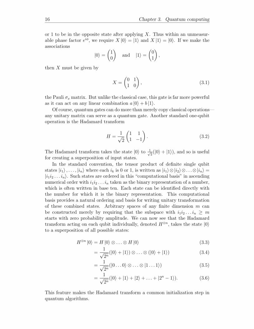
16 Chapter 3. Quantum computing
or 1 to be in the opposite state after applying X. Thus within an unmeasur-able phase factor eiφ, we require X |0〉 = |1〉 and X |1〉 = |0〉. If we make theassociations
|0〉 =
(10
)and |1〉 =
(01
),
then X must be given by
X =
(0 11 0
), (3.1)
the Pauli σx matrix. But unlike the classical case, this gate is far more powerfulas it can act on any linear combination a |0〉+ b |1〉.
Of course, quantum gates can do more than merely copy classical operations—any unitary matrix can serve as a quantum gate. Another standard one-qubitoperation is the Hadamard transform
H =1√2
(1 11 −1
). (3.2)
The Hadamard transform takes the state |0〉 to 1√2(|0〉+ |1〉), and so is useful
for creating a superposition of input states.
In the standard convention, the tensor product of definite single qubitstates |i1〉 , . . . , |in〉 where each ik is 0 or 1, is written as |i1〉⊗|i2〉⊗ . . .⊗|in〉 =|i1i2 . . . in〉. Such states are ordered in this “computational basis” in ascendingnumerical order with i1i2 . . . in taken as the binary representation of a number,which is often written in base ten. Each state can be identified directly withthe number for which it is the binary representation. This computationalbasis provides a natural ordering and basis for writing unitary transformationof these combined states. Arbitrary spaces of any finite dimension m canbe constructed merely by requiring that the subspace with i1i2 . . . in ≥ mstarts with zero probability amplitude. We can now see that the Hadamardtransform acting on each qubit individually, denoted H⊗n, takes the state |0〉to a superposition of all possible states:
H⊗n |0〉 = H |0〉 ⊗ . . .⊗H |0〉 (3.3)
=1√2n
(|0〉+ |1〉)⊗ . . .⊗ (|0〉+ |1〉) (3.4)
=1√2n
(|0 . . . 0〉 ⊗ . . .⊗ |1 . . . 1〉) (3.5)
=1√2n
(|0〉+ |1〉+ |2〉+ . . .+ |2n − 1〉). (3.6)
This feature makes the Hadamard transform a common initialization step inquantum algorithms.
3.4. Reversible computation 17
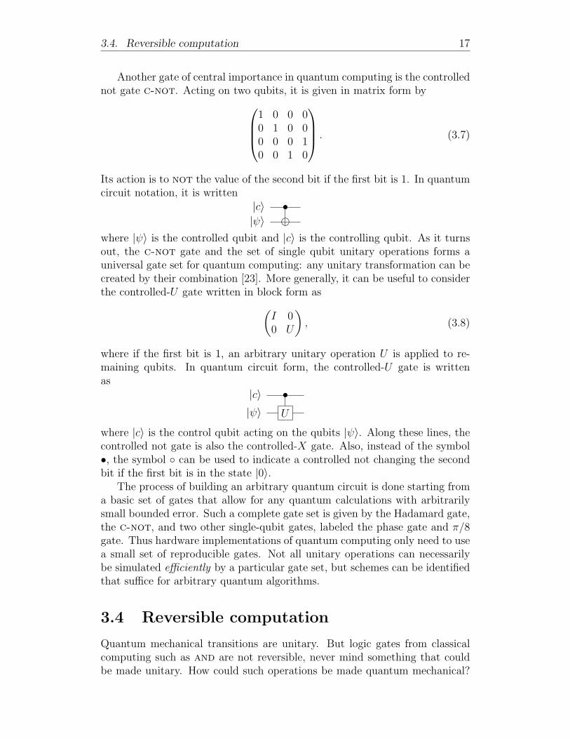
Another gate of central importance in quantum computing is the controllednot gate c-not. Acting on two qubits, it is given in matrix form by
1 0 0 00 1 0 00 0 0 10 0 1 0
. (3.7)
Its action is to not the value of the second bit if the first bit is 1. In quantumcircuit notation, it is written
|c〉 •|ψ〉
where |ψ〉 is the controlled qubit and |c〉 is the controlling qubit. As it turnsout, the c-not gate and the set of single qubit unitary operations forms auniversal gate set for quantum computing: any unitary transformation can becreated by their combination [23]. More generally, it can be useful to considerthe controlled-U gate written in block form as(
I 00 U
), (3.8)
where if the first bit is 1, an arbitrary unitary operation U is applied to re-maining qubits. In quantum circuit form, the controlled-U gate is writtenas
|c〉 •|ψ〉 U
where |c〉 is the control qubit acting on the qubits |ψ〉. Along these lines, thecontrolled not gate is also the controlled-X gate. Also, instead of the symbol•, the symbol can be used to indicate a controlled not changing the secondbit if the first bit is in the state |0〉.
The process of building an arbitrary quantum circuit is done starting froma basic set of gates that allow for any quantum calculations with arbitrarilysmall bounded error. Such a complete gate set is given by the Hadamard gate,the c-not, and two other single-qubit gates, labeled the phase gate and π/8gate. Thus hardware implementations of quantum computing only need to usea small set of reproducible gates. Not all unitary operations can necessarilybe simulated efficiently by a particular gate set, but schemes can be identifiedthat suffice for arbitrary quantum algorithms.
3.4 Reversible computation
Quantum mechanical transitions are unitary. But logic gates from classicalcomputing such as and are not reversible, never mind something that couldbe made unitary. How could such operations be made quantum mechanical?
18 Chapter 3. Quantum computing
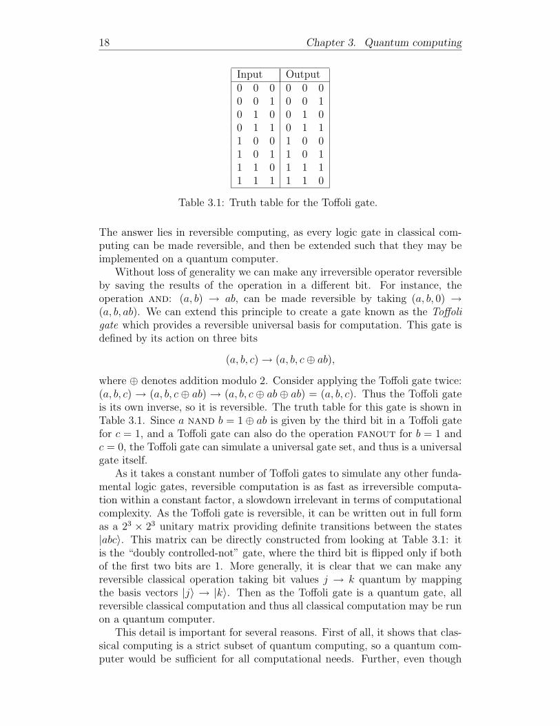
Input Output0 0 0 0 0 00 0 1 0 0 10 1 0 0 1 00 1 1 0 1 11 0 0 1 0 01 0 1 1 0 11 1 0 1 1 11 1 1 1 1 0
Table 3.1: Truth table for the Toffoli gate.
The answer lies in reversible computing, as every logic gate in classical com-puting can be made reversible, and then be extended such that they may beimplemented on a quantum computer.
Without loss of generality we can make any irreversible operator reversibleby saving the results of the operation in a different bit. For instance, theoperation and: (a, b) → ab, can be made reversible by taking (a, b, 0) →(a, b, ab). We can extend this principle to create a gate known as the Toffoligate which provides a reversible universal basis for computation. This gate isdefined by its action on three bits
(a, b, c)→ (a, b, c⊕ ab),
where ⊕ denotes addition modulo 2. Consider applying the Toffoli gate twice:(a, b, c) → (a, b, c ⊕ ab) → (a, b, c ⊕ ab ⊕ ab) = (a, b, c). Thus the Toffoli gateis its own inverse, so it is reversible. The truth table for this gate is shown inTable 3.1. Since a nand b = 1⊕ ab is given by the third bit in a Toffoli gatefor c = 1, and a Toffoli gate can also do the operation fanout for b = 1 andc = 0, the Toffoli gate can simulate a universal gate set, and thus is a universalgate itself.
As it takes a constant number of Toffoli gates to simulate any other funda-mental logic gates, reversible computation is as fast as irreversible computa-tion within a constant factor, a slowdown irrelevant in terms of computationalcomplexity. As the Toffoli gate is reversible, it can be written out in full formas a 23 × 23 unitary matrix providing definite transitions between the states|abc〉. This matrix can be directly constructed from looking at Table 3.1: itis the “doubly controlled-not” gate, where the third bit is flipped only if bothof the first two bits are 1. More generally, it is clear that we can make anyreversible classical operation taking bit values j → k quantum by mappingthe basis vectors |j〉 → |k〉. Then as the Toffoli gate is a quantum gate, allreversible classical computation and thus all classical computation may be runon a quantum computer.
This detail is important for several reasons. First of all, it shows that clas-sical computing is a strict subset of quantum computing, so a quantum com-puter would be sufficient for all computational needs. Further, even though
3.4. Reversible computation 19
all classical computation could just be run on a classical computer directly,the theoretical ability to mock up quantum versions of an any classical cir-cuit is important when considering minor adaptations of otherwise classicalalgorithms. This is important for the implementation of quantum walks asdiscussed in the following chapter.

Chapter 4
Quantum random walks
4.1 Markov chains and random walks
Before considering quantum random walks, it is worthwhile to recall the for-malism of classical random walks, embodied in the notion of a Markov chain.Consider any system undergoing random transitions between a discrete set ofpossibilities. Let a column vector p with each term positive and summing toone be a probability distribution over these states. For each possible state,there is corresponding column vector that gives the probability of transitionto each other state. Accordingly transitions to another state via a randomprocess can be described by a Markov transition matrix M where the ijthentry is given by
Mij = Pr(i|j), (4.1)
and the state after the random process is given by1
p′ = Mp. (4.2)
Repeated applications of the random process can be determined by repeatedleft multiplication by M .
For example, for the random walk on a line with equal probability of movingleft and right, the transition matrix is given by the band diagonal matrix
M =
. . .12
0 12
12
0 12
12
0 12
. . .
. (4.3)
1The standard convention of mathematicians for Markov chains uses right multiplication,but instead we use an equivalent formulation with left multiplication to emphasize theirconnection with changes of state in quantum mechanics.
22 Chapter 4. Quantum random walks
Thus a particle at position n goes to positions n − 1 and n + 1 each withprobability 1
2.
In general, Markov chains greatly aide the analysis of complicated randomsystems. For instance, stationary distributions can be identified immediatelyas the eigenvectors of M with eigenvalue 1. They are a widely used toolin probability theory, but for our purposes it will be sufficient to note theirexistence and form for comparison to quantum walks.
4.2 Defining a quantum walk
Equation (4.2) looks remarkably similar in form to the quantum mechanicalevolution of a state |ψ〉 under the unitary operator U ,
|ψ′〉 = U |ψ〉 , (4.4)
with the new normalization condition 〈ψ|ψ〉 = 1. Evolution after each addi-tional time steps proceeds again by left multiplication by U . But if projectivemeasurement onto basis state is performed after each application of U , theunitary transition U becomes a stochastic process that can be described by aMarkov chain, with a transition matrix given by entries
Mij = U∗ijUij = |Uij|2, (4.5)
corresponding to the ijth entry Uij of U . This “classical limit” is the naturalway in which a quantum operation suggests a random walk.
We call such an quantum system when thought of in the context of therandom walk that is its classical limit a quantum random walk. Originallyconsidered in continuous time and space in 1993 [4], quantum random walks indiscrete space have been the focus of subsequent work because they amenableto use in quantum algorithms. Although our focus is on quantum walks dis-crete in both time and space, there is significant literature concerning quantumwalks that evolve in continuous time. They will not be discussed here, butthey have similarly powerful algorithmic applications, including exponential topolynomial speedup for some contrived problems [10]. Thus in some sense—not very usefully—any quantum system can be considered as such a walk, soin practice systems are labeled quantum walks to emphasize their connectionwith classical walks.
The difficulty with this definition is that a quantum mechanical operationinduces a random walk, not the other way around. As the standard challengein quantum computing is to speed up classical algorithms, we would like to beable to directly find quantum analogs of classical walks. Any sort of randomwalk with discrete positions marked on a graph is a natural candidate. Thefocus of research in this subfield has been to discover quantum versions ofclassical walks of interest and examine the distinctions between quantum andclassical versions, all with an eye toward “speeding up” algorithms based onsuch walks.
4.3. Quantum walks on a line 23
We will introduce quantum walks and their uses in the remainder of thischapter. For further details and more applications, we recommend that theinterested reader consult review articles by Ambainis [5] and Kempe [16].
4.3 Quantum walks on a line
The simplest classical random walk is a particle on a discrete line in onedimension. At each step, a coin is flipped and the particle moves left orright with equal probability. The transition matrix for this walk was givenpreviously in Equation (4.3), and the probability distribution from this walkis well known to proceed as a binomial distribution. The probability of findingthe particle at position n at time T p(n, T ) is zero if n+T is odd and otherwisegiven by
p(n, T ) =1
2T
(T
12(n+ T )
), if n+ T even (4.6)
where the deviation from the direct binomial distribution(Tn
)arises because
the walking particle moves left or right dependent on a coin flip, instead ofmerely moving on each successful flip. In any case the distribution for this walkis identical to the binomial distribution centered at the origin adding zeros atalternate positions. Over time, the average position 〈n〉 = 0 and the variance,the average distance squared to the mean, is given by σ2 = 〈(n − 〈n〉)2〉 =〈n2〉 = T , as can be show by straightforward algebra.
Since so much of the representative power of the classical random walk isfound on the line, the line is a natural first candidate for finding a quantumrandom walk as well. Following the definition given in the proceeding section,we would like to find a quantum walk on the line with a random walk as itsclassical limit.
The most obvious way to define a quantum walk on a line is to choose asa set of basis states |n〉, n ∈ Z representing each integer. Then we would liketo find a unitary operator U that acts as a classical walk under measurement.The operation should act identically on each position state |n〉 by altering theposition with some probability. Defining its action on each basis vector |n〉,then the walk must be given by some U such that
U |n〉 = a |n− 1〉+ b |n〉+ c |n+ 1〉 , (4.7)
where a, b, c ∈ C. However, defining a non-trivial quantum walk in this manneris not possible, as the following theorem shows.
Theorem. If this operation U as defined above is unitary, then exactly one ofthe following holds (a simple case following the general proof given by Meyer[19]):
1. |a|2 = 1, b = c = 0

24 Chapter 4. Quantum random walks
2. |b|2 = 1, a = c = 0
3. |c|2 = 1, a = b = 0
Proof. Written in matrix form, we have
U =
. . . a
b ac b a
c b
c. . .
.
Since the columns of U form an orthonormal set, we have
c∗a = 0
a∗b+ b∗c = 0
|a|2 + |b|2 + |c|2 = 1.
From the first two equations, at least two of a, b and c must equal zero, andby the last equation one of the cases 1-3 is fulfilled.
Accordingly if a walk is defined as in Equation (4.7) at each step a particlemakes a definite step left or right, or stays in the same position. These are notinteresting cases, but fortunately, non-trivial quantum walks can be easily de-fined using only slightly more complicated operations. There are multiple waysin which this could be done; here we present only the most straightforwardand extensible method, known as the “coined” quantum walk.
The walk is performed on the Hilbert space Hs ⊗ Hc, the tensor productof Hilbert space Hs of discrete position states |n〉 with another 2-dimensionalspace Hc labeled the coin space. We label a set of orthonormal basis vectors inHc as |−〉 and |+〉. Thus the coin space is equivalent to the particle having spin-12. Two unitary operations are then defined which are performed in succession
at each time step.
1. The “coin flip” operator C acts on Hc:
C |−〉 = a |−〉+ b |+〉 (4.8a)
C |+〉 = c |−〉+ d |+〉 (4.8b)
2. The “shift” operator S applies a conditional shift to the states |n〉 de-pendent on the coin state:
S |n,−〉 = |n− 1,−〉 (4.9a)
S |n,+〉 = |n+ 1,+〉 (4.9b)
4.3. Quantum walks on a line 25
The evolution of the walk in one time step is thus given by U = S · (I ⊗ C).The operator I ⊗ C indicates the identity operation on the position subspaceand the operation C on the coin subspace, and is unitary for any unitary C =(a bc d
). The operator S is also clearly unitary since it is norm preserving as it
merely exchanges the amplitudes associated with basis vectors. Accordinglythe evolution U is unitary as well.
The coin flip operator C may be specified by any unitary matrix. Standardchoices include the Hadamard transformation
H =1√2
(1 11 −1
)(4.10)
and the “balanced” coin
Y =1√2
(1 ii 1
). (4.11)
Both these operators exactly reproduce the classical random walk in the clas-sical limit when projective measurement is applied after each set to collapsethe state |ψ〉 to a state with definite number |n〉, since any state specifiedby |n〉 transitions to either |n− 1〉 or |n+ 1〉 with equal probability. Nowconsider the evolution of an initial state |ψ〉 = |0,+〉 using the Hadamardtransformation H as the coin operator:
|ψ〉 → 1√2|−1,−〉 − 1√
2|1,+〉 (4.12a)
→ 1
2|−2,−〉 − 1
2|0,−〉+
1
2|0,+〉+
1
2|2,+〉 (4.12b)
→ 1
2√
2|−3,−〉+
1
2√
2|−1,+〉+
1√2|−1,−〉 − 1
2√
2|1,−〉+
1
2√
2|3,+〉
(4.12c)
After the first two evolutions, the probability of measuring the particle at anyposition remains the same as for a classical random walk. But on the thirdapplication of U , positive moving amplitudes at n = 1 interfere destructivelysimultaneously with constructive interference at n = −1. There is a probabil-ity 5/8 of the particle being measured in the state |−1〉 but only a probability1/8 at |1〉. Quantum effects have entered our random walk, and all futureevolution of the walk will show even more interference effects.
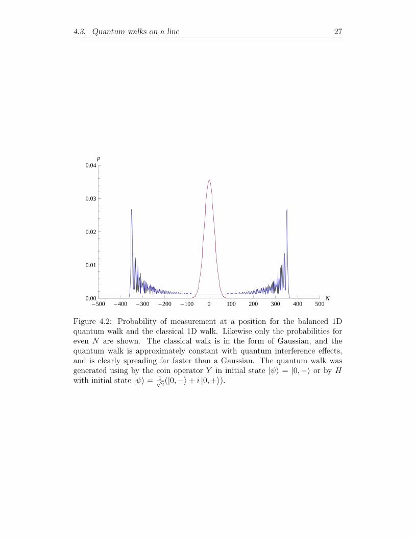
Graphs of the probability distribution of these walks initialized in the state|ψ〉 = |0,−〉 as measured after T steps are shown in Figure 4.1. The Hadamardmatrix is real, but does not treat |−〉 and |+〉 state symmetrically and thusleads to an asymmetric walk as shown when started in a state initially movingstrictly in one direction. The initial state |ψ〉 = |0,+〉 leads to the sameprobability distribution reflected over the vertical axis, so the initial state|ψ〉 = 1√
2(|0,−〉+i |0,+〉) with the coin H leads to the symmetrical probability
distribution shown in Figure 4.2, since H has all real values, so the imaginary
26 Chapter 4. Quantum random walks
-500 -400 -300 -200 -100 0 100 200 300 400 500N0.00
0.01
0.02
0.03
0.04p
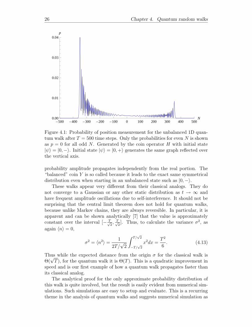
Figure 4.1: Probability of position measurement for the unbalanced 1D quan-tum walk after T = 500 time steps. Only the probabilities for even N is shownas p = 0 for all odd N . Generated by the coin operator H with initial state|ψ〉 = |0,−〉. Initial state |ψ〉 = |0,+〉 generates the same graph reflected overthe vertical axis.
probability amplitude propagates independently from the real portion. The“balanced” coin Y is so called because it leads to the exact same symmetricaldistribution even when starting in an unbalanced state such as |0,−〉.
These walks appear very different from their classical analogs. They donot converge to a Gaussian or any other static distribution as t → ∞ andhave frequent amplitude oscillations due to self-interference. It should not besurprising that the central limit theorem does not hold for quantum walks,because unlike Markov chains, they are always reversible. In particular, it isapparent and can be shown analytically [7] that the value is approximatelyconstant over the interval [− T√
2, T√
2]. Thus, to calculate the variance σ2, as
again 〈n〉 = 0,
σ2 = 〈n2〉 =1
2T/√
2
∫ T/√
2
−T/√
2
x2dx =T 2
6. (4.13)
Thus while the expected distance from the origin σ for the classical walk isΘ(√T ), for the quantum walk it is Θ(T ). This is a quadratic improvement in
speed and is our first example of how a quantum walk propagates faster thanits classical analog.
The analytical proof for the only approximate probability distribution ofthis walk is quite involved, but the result is easily evident from numerical sim-ulations. Such simulations are easy to setup and evaluate. This is a recurringtheme in the analysis of quantum walks and suggests numerical simulation as
4.3. Quantum walks on a line 27
-500 -400 -300 -200 -100 0 100 200 300 400 500N0.00
0.01
0.02
0.03
0.04p
Figure 4.2: Probability of measurement at a position for the balanced 1Dquantum walk and the classical 1D walk. Likewise only the probabilities foreven N are shown. The classical walk is in the form of Gaussian, and thequantum walk is approximately constant with quantum interference effects,and is clearly spreading far faster than a Gaussian. The quantum walk wasgenerated using by the coin operator Y in initial state |ψ〉 = |0,−〉 or by Hwith initial state |ψ〉 = 1√
2(|0,−〉+ i |0,+〉).
28 Chapter 4. Quantum random walks
the primary method of attack for these problems. Once a result is obtainednumerically, then it may be well worth attempting to prove analytically.
4.4 Quantum walks on regular graphs
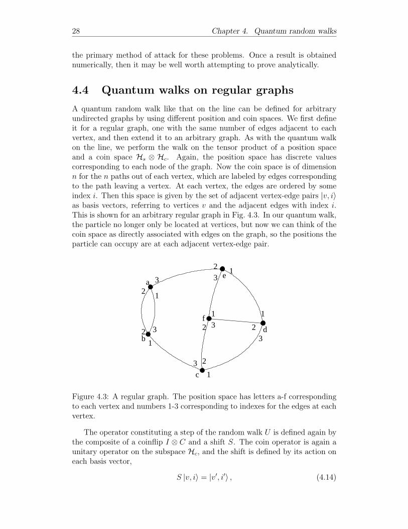
A quantum random walk like that on the line can be defined for arbitraryundirected graphs by using different position and coin spaces. We first defineit for a regular graph, one with the same number of edges adjacent to eachvertex, and then extend it to an arbitrary graph. As with the quantum walkon the line, we perform the walk on the tensor product of a position spaceand a coin space Hs ⊗ Hc. Again, the position space has discrete valuescorresponding to each node of the graph. Now the coin space is of dimensionn for the n paths out of each vertex, which are labeled by edges correspondingto the path leaving a vertex. At each vertex, the edges are ordered by someindex i. Then this space is given by the set of adjacent vertex-edge pairs |v, i〉as basis vectors, referring to vertices v and the adjacent edges with index i.This is shown for an arbitrary regular graph in Fig. 4.3. In our quantum walk,the particle no longer only be located at vertices, but now we can think of thecoin space as directly associated with edges on the graph, so the positions theparticle can occupy are at each adjacent vertex-edge pair.
1
2
3
21
3
32
1
1
1
1
2
3
3 2
2 3
a
b
c
d
e
f
Figure 4.3: A regular graph. The position space has letters a-f correspondingto each vertex and numbers 1-3 corresponding to indexes for the edges at eachvertex.
The operator constituting a step of the random walk U is defined again bythe composite of a coinflip I ⊗ C and a shift S. The coin operator is again aunitary operator on the subspace Hc, and the shift is defined by its action oneach basis vector,
S |v, i〉 = |v′, i′〉 , (4.14)
4.4. Quantum walks on regular graphs 29
where v′ is the other vertex attached to edge marked by i, and i′ is the labelingfor the index associated with the same edge marked by i. There are many waysin which the index i may be ordered at each vertex. As in Fig. 4.3, it may bechosen arbitrarily, but more generally, when possible, it is chosen in some waythat reflects the symmetry of the graph, or in which i and i′ may be labeledthe same. For instance on a square lattice, indexes , , and would bechosen corresponding to the direction of each path.
In general, the coin operator C may also be chosen arbitrarily, but two suchchoices are most common. The first such coin is the discrete Fourier transform(DFT). Recall that the Fourier Transform X(f) is given by
X(f) =
∫ ∞−∞
x(t)e−2πiftdt. (4.15)
Then the discrete Fourier transform ~X ∈ Cn performs the same transformationas the Fourier Transform on the discrete set of n data points ~x ∈ Cn by
Xk =1√n
n−1∑j=0
xje−2πijk/n (4.16)
with the substitutions t→ j, dt→ 1 and f → k/n. The factor 1/√n in front
is a normalization constant so that ~x and ~X have the same length, making theDFT transformation unitary, as can be easily verified. Then we can re-expressthe DFT as mapping basis vectors |j〉 to |k〉 as with
|j〉 → 1√n
n−1∑k=0
e2πijk/n |k〉 , (4.17)
which in matrix form in the standard basis gives us,
DFT =1√n
1 1 1 · · · 11 γ γ2 · · · γn−1
1 γ2 γ4 · · · γ2(n−1)
......
.... . .
...1 γn−1 γ2(n−1) · · · γ(n−1)(n−1)
, (4.18)
where γ = e2πi/n is the nth root of unity. It turns out that the DFT gatecan in general be constructed easily out of simple gates for use in a quantumcomputer [23]. This gate makes it easy to find the periodicity of functions,and is the basis of a whole family of quantum algorithms based off Shor’srevolutionary algorithm for integer factorization in time O(poly) in contrastto the best classical algorithm running in time O(exp). But this operationis also remarkably useful for quantum walks. In some sense it is the naturalgeneralization of the Hadamard transformation (Eq. (4.10)), as the Hadamardtransform is the discrete Fourier transform with n = 2. In the classical limit

30 Chapter 4. Quantum random walks
this coin gives an equal probability of a transition from any state to any other,since each matrix element has equal absolute value, and this operation is theunique such choice, up to an irrelevant phase factor and permutation of therows and columns. This coin lets us exactly reproduce a random walk on agraph with equal probability of moving along each edge from a vertex, but itintroduces phase differences dependent upon the path. These phases break thesymmetry of the original random walk, just as in the case of the Hadamardcoin H vs. the balanced coin Y (Eq. (4.11)), but for n > 2 there is not aneasy way to account for this lack of balance with a difference initial state.
The second coin of prominent use is an extension of the balanced coin Y .It is also, perhaps not coincidently, an operation of central importance in theother main family of quantum algorithms. Physically, a particle in a quantumwalk can be considered to be moving through the graph and scattering off avertex. If the coin matrix corresponds to a physical operation of scattering,then the resulting amplitude distribution should respect the symmetry of theinteraction. So the balanced coin reflects the symmetry of a random walk ona line in a way that the Hadamard coin does not by treating the transitionsfrom positive to negative moving particles and vice-versa symmetrically. Theseare also the sort of coins that yield quantum walks corresponding to physicalprocess, such as discrete versions of the Schrodinger and Dirac equations. Forexample, a quantum walk on a square lattice, on the basis |〉 , |〉 , |〉 , |〉corresponding to shifts in the direction of the arrow, one would expect a coinof the form
C =
a c b cc a c bb c a cc b c a
, (4.19)
as particles arriving in any direction at a vertex should have the same ampli-tudes associated with reflection (a), transmission (b) or deflection to the leftor right at 90 degrees (c).
For a general graph without any additional structure, there is only onefeature that breaks the symmetry of the problem: the edge along which aprobability amplitude representing a particle arrives. Then coins respectingthis symmetry would be matrices of the form
C =
a b · · · bb a · · · b...
.... . .
...b b · · · a
(4.20)
at each vertex, with some constant amplitude a for the diagonal elements andb for the off-diagonal elements. The constant off-diagonal elements associatethe same amplitude with each possible edge change. Using the requirement

4.4. Quantum walks on regular graphs 31
that this matrix must be unitary, we can place restrictions on a and b. By theorthonormality of the columns,
|a|2 + (n− 1)|b|2 = 1 (4.21a)
a∗b+ b∗a+ (n− 2)|b|2 = 0. (4.21b)
Let α = |a| and β = |b| be the magnitudes of a and b. Then action of thecoin will clearly only depend upon the phase difference ∆ between a and b asany overall phase can be factored out of the matrix, and phase factors are notmeasurable. Then as a∗b+ b∗a = 2αβ cos ∆, we have
α2 + (n− 1)β2 = 1 (4.22a)
2αβ cos ∆ + (n− 2)β2 = 0. (4.22b)
For n = 2, there are three solutions: the identity, the Pauli matrix σx andsymmetric coin Y from Eq. (4.11). Solving these equations for α and β yieldsa continuum of solutions for n > 2. These are given by
α =
(1 +
4(n− 1) cos ∆
(n− 2)2
)−1/2
(4.23a)
β =2α cos ∆
n− 2. (4.23b)
These solutions are shown graphically in Fig 4.4. As ∆ → π/2, that is as aand b become orthogonal vectors in the complex plane, β → 0, so the coin issome multiple of the identity. As ∆ → 0, a and b becomes parallel vectors,yielding another solution that can be written as a real matrix (clearly a andb will have to differ in sign). Making an arbitrary sign choice, the case ∆ = 0simplifies to the diffusion operator G from Grover’s search algorithm,
G =
−1 + 2
n2n
· · · 2n
2n
−1 + 2n· · · 2
n...
.... . .
...2n
2n
· · · −1 + 2n
, (4.24)
Α
Β
0 Π
8
Π
4
3 Π
8Π
2
D0
0.5
1
Figure 4.4: Magnitudes of diagonal elements α and non-diagonal elements βas a function of the phase difference ∆ with n = 5.
32 Chapter 4. Quantum random walks
which can also be written
G = −I + 2 |ψ〉〈ψ| , (4.25)
where |ψ〉 = 1√n
∑ni=0 |i〉 is the equal superposition over all states. This choice
of “Grover’s coin” ensures that amplitudes spreads through a quantum walkat the maximum rate, as using the identity operator as a coin means that thewalk does not move at all. Clearly as n increases, all these solutions includ-ing Grover’s coin tend strictly toward the identity operator, but this cannotbe avoided, and as it turns out, does not mean that this coin is necessarilyless powerful than the classical “fair” coin with equal transition probabilities.On general graphs, in addition to being more physically realistic, these sortsof coins are more likely to creating interesting quantum walks, as respectingthe symmetry of the graph allows quantum interference to yield non-classicalresults. Another advantage of this particular coin is that the matrix has sub-stantial symmetry that could make analytical analysis substantially easier.
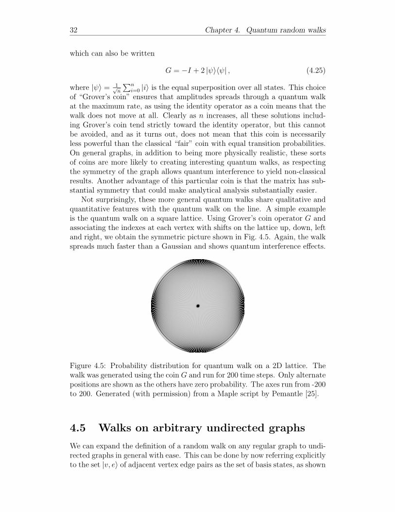
Not surprisingly, these more general quantum walks share qualitative andquantitative features with the quantum walk on the line. A simple exampleis the quantum walk on a square lattice. Using Grover’s coin operator G andassociating the indexes at each vertex with shifts on the lattice up, down, leftand right, we obtain the symmetric picture shown in Fig. 4.5. Again, the walkspreads much faster than a Gaussian and shows quantum interference effects.
Figure 4.5: Probability distribution for quantum walk on a 2D lattice. Thewalk was generated using the coin G and run for 200 time steps. Only alternatepositions are shown as the others have zero probability. The axes run from -200to 200. Generated (with permission) from a Maple script by Pemantle [25].
4.5 Walks on arbitrary undirected graphs
We can expand the definition of a random walk on any regular graph to undi-rected graphs in general with ease. This can be done by now referring explicitlyto the set |v, e〉 of adjacent vertex edge pairs as the set of basis states, as shown
4.6. Quantum walks on quantum computers 33
a
109
87
6
5
4
3
2
1 g
f
e
dc
b
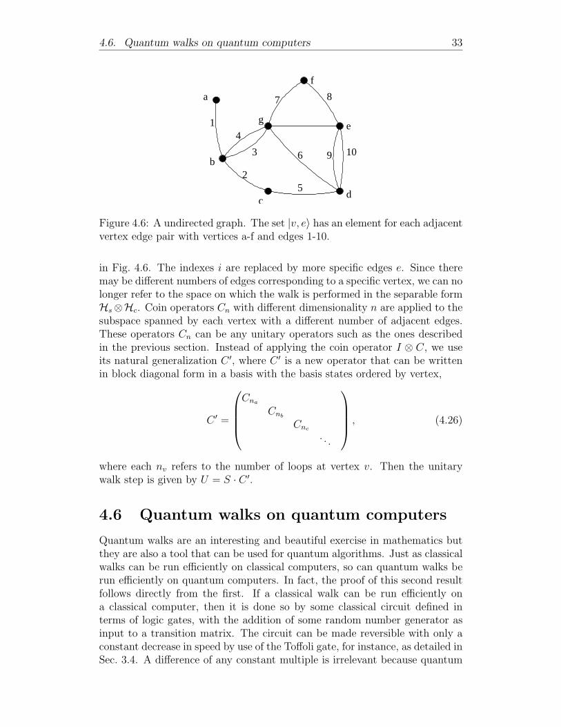
Figure 4.6: A undirected graph. The set |v, e〉 has an element for each adjacentvertex edge pair with vertices a-f and edges 1-10.
in Fig. 4.6. The indexes i are replaced by more specific edges e. Since theremay be different numbers of edges corresponding to a specific vertex, we can nolonger refer to the space on which the walk is performed in the separable formHs⊗Hc. Coin operators Cn with different dimensionality n are applied to thesubspace spanned by each vertex with a different number of adjacent edges.These operators Cn can be any unitary operators such as the ones describedin the previous section. Instead of applying the coin operator I ⊗ C, we useits natural generalization C ′, where C ′ is a new operator that can be writtenin block diagonal form in a basis with the basis states ordered by vertex,
C ′ =
Cna
Cnb
Cnc
. . .
, (4.26)
where each nv refers to the number of loops at vertex v. Then the unitarywalk step is given by U = S · C ′.
4.6 Quantum walks on quantum computers
Quantum walks are an interesting and beautiful exercise in mathematics butthey are also a tool that can be used for quantum algorithms. Just as classicalwalks can be run efficiently on classical computers, so can quantum walks berun efficiently on quantum computers. In fact, the proof of this second resultfollows directly from the first. If a classical walk can be run efficiently ona classical computer, then it is done so by some classical circuit defined interms of logic gates, with the addition of some random number generator asinput to a transition matrix. The circuit can be made reversible with only aconstant decrease in speed by use of the Toffoli gate, for instance, as detailed inSec. 3.4. A difference of any constant multiple is irrelevant because quantum

34 Chapter 4. Quantum random walks
|v〉 /
S
T
|e〉 / C
Figure 4.7: Quantum circuit implementation of a quantum walk on a regulargraph. The walk operation U is outlined by the box marked by T , to indicatethat the circuit inside is repeated sequentially T times. There are qubitsrepresenting the vertices |v〉 and the edges |e〉, and the gates marked C and Sare the coin and shift operations.
and classical hardware will differ massively in speed and design anyways. Thenin place of using a stochastic transition between states, we place the “coin flip”operator directly into the quantum circuit instead.
More concretely, we can also create a quantum circuit diagrams for anarbitrary quantum walk that show directly how they could be implementedon a quantum computer. Such a diagram is shown in Fig. 4.7. For simplicity,it shows a quantum walk on a regular graph; the implementation of a generalundirected graph is similar, although it is harder to draw the circuit clearly.
Chapter 5
Quantum walk search
In previous chapters we have presented both random walk search based algo-rithms for k-SAT and quantum random walks as a family of algorithms thatcan be faster than classical random walks. The challenge discussed in thischapter and the next is to find faster quantum versions of these randomizedalgorithms.
5.1 Quantum search
Searching a database is a basic and essential task for computers. In the classicalworld, finding a particular entry in an unsorted database of N items alwaystakes on average checkingN/2 entries. So classical database search runs in timeO(N). In contrast, Lov Grover’s search algorithm can search any unstructureddatabase by with only O(
√N) queries of an Oracle f(x) [23]. This result is
remarkable because almost every important algorithm in classical computingcan be phrased as a search of some sort, even if it works as naively as bychecking every possible solution. The quadratic speedup offered by Grover’salgorithm has been proved to be the best possible result for general search.
But real databases have their entries stored in physical media. It is fareasier to flip to the next page of this thesis than to head to the library andcheck out another book, and it takes more effort to flip two pages than onepage. Moreover, information may be transmitted no faster than the speedof light, and actual quantum circuits will take time to look up entries. Soas a new model, consider search of a database on a graph with one entry ateach point. Then instead of reading all entries simultaneously, we imagine a“quantum robot” moving through the database in the form of operations thatcan only be applied locally [8]. If this robot is running Grover’s algorithm,it will take M times longer to run the search algorithm, where M is averagedistance it needs to move between vertices. It still only requires only O(
√N)
queries, but between each evaluation it takes M steps to move to the nextvertex. More precisely, the Oracle operation itself now takes O(M) steps toevaluate. Then as a square grid of N elements has distance O(
√N) between
36 Chapter 5. Quantum walk search
elements, running Grover’s search on this structured database in fact takesorder
√N ×
√N = N steps, no better than classical search [11].
Quantum walks resolve this issue by providing a means to perform localsearch on structured databases often just as fast as Grover’s algorithm. Thequantum walk by analogy has robots as cellular automata stuck at each cellwho can only pass quantum states off to their neighbors. These search al-gorithms are remarkably simple and have been implemented for a variety ofgraphs reaching the theoretical limit of O(
√N) performance or close to it
for many graphs. Aaronson and Ambainis have shown that for 3 or moredimensions, quantum search on a grid can be performed in time O(
√N), al-
though their best algorithm for search on the 2 dimensional lattice is in time
O(√
N log3/2N)
[2].
5.2 Binary hypercube search
Quantum walk search works on many graphs, but search on most graphs lacksan algorithmic application. Recall the binary hypercube in n-dimensions, asintroduced in the discussion of satisfiable algorithms in Sec. 2.3. We can con-sider this graph as a database with N = 2n entries. One vertex x0 chosenarbitrarily is marked as the solution to our search. Classically, starting fromany initial vertex, it takes O(2n) steps until a solution is reached with highprobability. Since the maximum distance between any two vertices is M = n,Grover’s algorithm could search the hypercube in O(n
√2n) steps. The fol-
lowing algorithm, due to Shevi, Kempe and Whaley [28], performs the spatialsearch in O(
√2n) steps.
Since the hypercube is regular, we can choose a basis by the vertices andan index keeping track of each edge. The set of basis vectors is of the form|x, i〉 ∈ Hs ⊗ Hc, where each vertex is a string of bits x, and the indexes icorrespond to the ith variable being flipped between the two adjacent vertices.In general, one arbitrary vertex x0 is marked as the solution. The algorithmis given as follows:
1. The system is initialized in the equal superposition state 1√n2n
∑x,i |x, i〉,
as can be obtained by performing a Hadamard transform on each qubitrepresenting the space Hs and Hc.
2. The operation U = S · C ′ is applied for π2
√2n steps.
(a) At unmarked vertices, the coin C0 is used. At the marked vertex,the coin C1 is used. Then the operation C ′ is given by
C ′ = I ⊗ C0 + |x0〉 〈x0| ⊗ (C1 − C0). (5.1)
Let C0 = G (Grover’s operator from Eq. (4.24)) and C1 = −I.
5.2. Binary hypercube search 37
0 20 40 60 80 100 120 140T0.0
0.1
0.2
0.3
0.4
0.5p
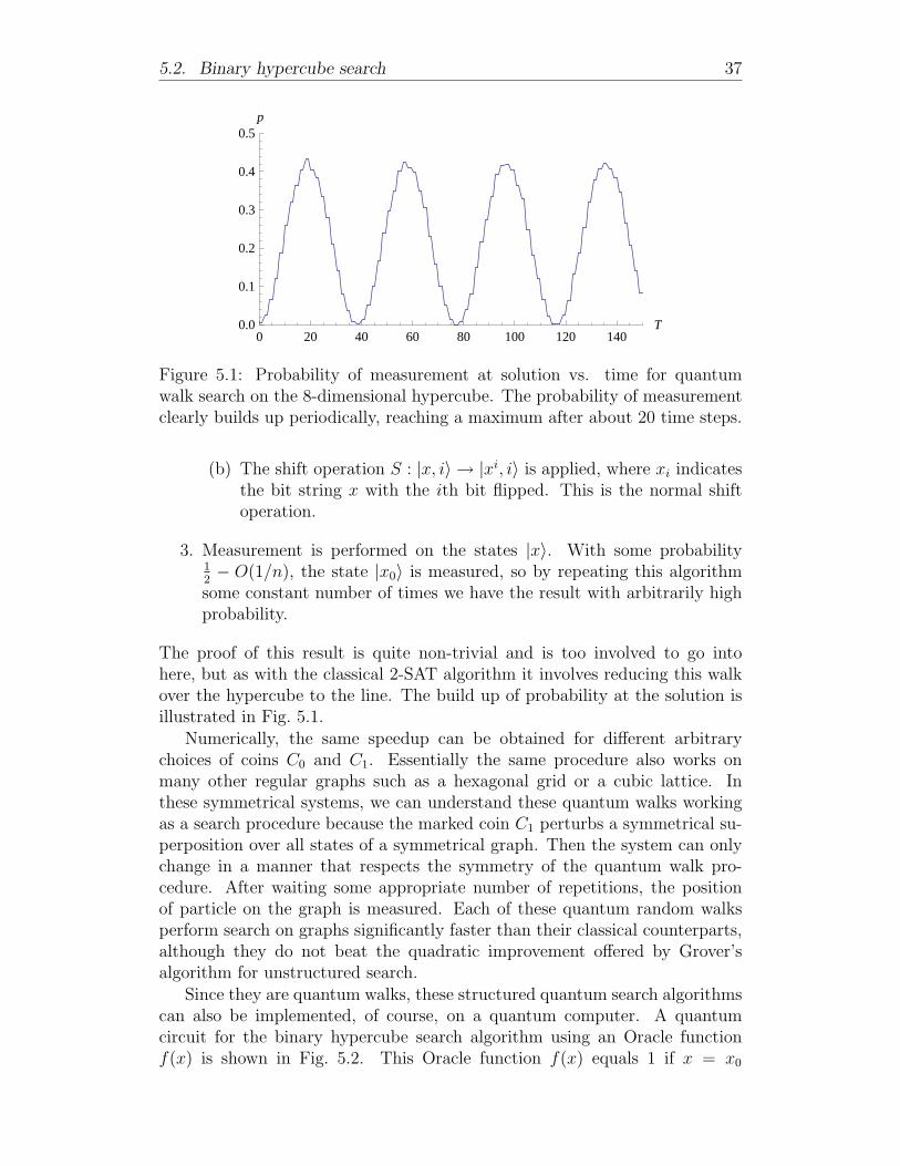
Figure 5.1: Probability of measurement at solution vs. time for quantumwalk search on the 8-dimensional hypercube. The probability of measurementclearly builds up periodically, reaching a maximum after about 20 time steps.
(b) The shift operation S : |x, i〉 → |xi, i〉 is applied, where xi indicatesthe bit string x with the ith bit flipped. This is the normal shiftoperation.
3. Measurement is performed on the states |x〉. With some probability12− O(1/n), the state |x0〉 is measured, so by repeating this algorithm
some constant number of times we have the result with arbitrarily highprobability.
The proof of this result is quite non-trivial and is too involved to go intohere, but as with the classical 2-SAT algorithm it involves reducing this walkover the hypercube to the line. The build up of probability at the solution isillustrated in Fig. 5.1.
Numerically, the same speedup can be obtained for different arbitrarychoices of coins C0 and C1. Essentially the same procedure also works onmany other regular graphs such as a hexagonal grid or a cubic lattice. Inthese symmetrical systems, we can understand these quantum walks workingas a search procedure because the marked coin C1 perturbs a symmetrical su-perposition over all states of a symmetrical graph. Then the system can onlychange in a manner that respects the symmetry of the quantum walk pro-cedure. After waiting some appropriate number of repetitions, the positionof particle on the graph is measured. Each of these quantum random walksperform search on graphs significantly faster than their classical counterparts,although they do not beat the quadratic improvement offered by Grover’salgorithm for unstructured search.
Since they are quantum walks, these structured quantum search algorithmscan also be implemented, of course, on a quantum computer. A quantumcircuit for the binary hypercube search algorithm using an Oracle functionf(x) is shown in Fig. 5.2. This Oracle function f(x) equals 1 if x = x0

38 Chapter 5. Quantum walk search
|c〉 c
x
Oracle
c⊕ f(x)
x
• c
x
Oracle
c⊕ f(x)
x
T
|x〉 / H⊗n x
i
S
xi
i
NM
|i〉 / H⊗(logn) C0 C1
Figure 5.2: Quantum circuit implementation of binary hypercube search al-gorithm. The control qubit |c〉 is initialized in the state |0〉 as are the qubitsreferred to by the labels |x〉 and |i〉. The position states |x〉 are stored in a setof n-qubits and the coin index |i〉 can without loss of generality be representedby log n qubits since it needs to have n distinct states. The Oracle circuitflips the value of |c〉 if x = x0 and is run again after the controlled operationsto reset the value of |c〉. The walk step U marked by the box is repeatedT = O(
√2n) times.
and 0 otherwise, and is the standard way in which a particular element ismarked in quantum algorithms. Writing the Oracle as circuit element suggeststhe approach we will use for satisfiability problems in which case the Oraclefunction actually involves the evaluation of a circuit, the formula for the SATproblem. The Oracle is in fact called twice for each iteration to reverse itsaction on the control qubit, but again some reduction in speed by a constantmultiple is irrelevant in a broader sense.
5.3 Converting hypercube search to k-SAT
Our challenge now is to adapt this quantum search procedure to solve sat-isfiability problems. However, there are a significant differences between thehypercube search problem and the k-SAT random walk algorithms. The k-SAT algorithms run on directed graphs with possibly redundant paths, ona subset of the binary hypercube. It is also possible and common to havemultiple solutions. Furthermore, several steps in the procedure such as theinitialization step rely on the symmetric nature and known structure of thegraph at each vertex. None of these challenges is necessarily insurmountablebut a quantum version of this walk will clearly be far less trivial on the hy-percube. As a general principle, even without proof or any particular reason,we can safely assume that no altering of the graph in the process of making itsuitable for quantum walks would improve the speed of the classical algorithm,or the approach would already have been taken. Under this principle, we willconsider two main approaches. The first is explained in the remainder of thischapter and the second in Chapter 6.
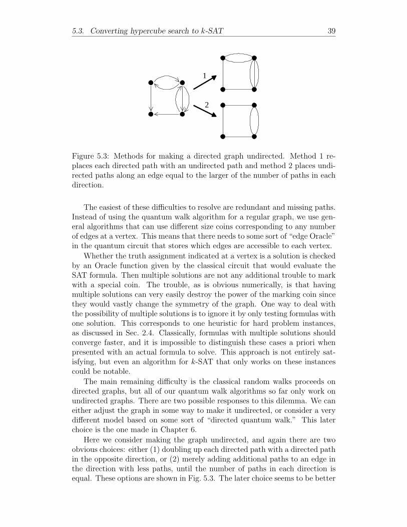
5.3. Converting hypercube search to k-SAT 39
2
1
Figure 5.3: Methods for making a directed graph undirected. Method 1 re-places each directed path with an undirected path and method 2 places undi-rected paths along an edge equal to the larger of the number of paths in eachdirection.
The easiest of these difficulties to resolve are redundant and missing paths.Instead of using the quantum walk algorithm for a regular graph, we use gen-eral algorithms that can use different size coins corresponding to any numberof edges at a vertex. This means that there needs to some sort of “edge Oracle”in the quantum circuit that stores which edges are accessible to each vertex.
Whether the truth assignment indicated at a vertex is a solution is checkedby an Oracle function given by the classical circuit that would evaluate theSAT formula. Then multiple solutions are not any additional trouble to markwith a special coin. The trouble, as is obvious numerically, is that havingmultiple solutions can very easily destroy the power of the marking coin sincethey would vastly change the symmetry of the graph. One way to deal withthe possibility of multiple solutions is to ignore it by only testing formulas withone solution. This corresponds to one heuristic for hard problem instances,as discussed in Sec. 2.4. Classically, formulas with multiple solutions shouldconverge faster, and it is impossible to distinguish these cases a priori whenpresented with an actual formula to solve. This approach is not entirely sat-isfying, but even an algorithm for k-SAT that only works on these instancescould be notable.
The main remaining difficulty is the classical random walks proceeds ondirected graphs, but all of our quantum walk algorithms so far only work onundirected graphs. There are two possible responses to this dilemma. We caneither adjust the graph in some way to make it undirected, or consider a verydifferent model based on some sort of “directed quantum walk.” This laterchoice is the one made in Chapter 6.
Here we consider making the graph undirected, and again there are twoobvious choices: either (1) doubling up each directed path with a directed pathin the opposite direction, or (2) merely adding additional paths to an edge inthe direction with less paths, until the number of paths in each direction isequal. These options are shown in Fig. 5.3. The later choice seems to be better
40 Chapter 5. Quantum walk search
for a two marginal reasons. First, it alters the classical algorithm less, as thereare less additional paths added into the graph, so the transition probabilities inthe classical limit would be altered by a lesser amount. Secondly, it would alsohave marginally less significant resource requirements for implementation, bothon a quantum device and for simulating performance on a classical computer.Nonetheless, we will look at both approaches.
Unfortunately, both of these approaches, and any based on an undirectedwalk, would not work in the classical limit. This is because the random walkSAT algorithms we have examined rely on solution vertices having no pathsout to trap random walk attempts there. When the graph is made undi-rected, the structure does not force the particle to stay at potential solutions,as undirected graphs always have the same number of edges in and out ofeach vertex. It appears that our quantum search algorithms and the classicalstructured search for SAT problems may rely on antithetical principles.
Still, we will evaluate the merit of this procedure experimentally. Nowthat we have an undirected graph on which to perform a quantum walk, weconsider the walk using the general formalism for undirected walks discussedin the previous chapter. Instead of using the same coins C0 and C1, we use thecoins of the same form scaled at each vertex to the number of attached edges.We also need to initialize graph in some uniform state that is not dependentupon the structure, as the walk possessing non-local knowledge of the locationof each path would require already having solved the problem. To do so, wecreate an equal superposition at each vertex such that the probability of thewalk starting at each vertex is the same, even if the edges from distinct verticesstart with different values.
There is one major distinction with the choice of marking coins from thehypercube search algorithm. In the original hypercube search, the coin C1 =−G produces identical results to the coin C1 = −I. This is because the walkis initialized in an entirely symmetric state, the amplitude on each vertex willalways be some multiple a of the equal superposition state |ψ〉. Then usingthe form of G from Eq. (4.25),
−Ga |ψ〉 = −(−I + 2 |ψ〉〈ψ|)a |ψ〉 = a |ψ〉 , (5.2)
so the equal superposition |ψ〉 is an eigenvector of the operator −G with eigen-value −1. Since the walk is initialized in this eigenstate, the operator has thesame action as the operator −I. In contrast, on these hypercube walks fork-SAT, the symmetry of the graphs has been thrown off in some way. Accord-ingly it is now possible that these two coin may result in different walks.
The full procedure for the algorithm is as follows:
1. Initialize walk in a uniform state equally likely to be at any vertex.
2. The operation U = S · C ′ is applied for t steps.
(a) Using an edge Oracle from the classical algorithm, record the edgesadjacent to each vertex from the classical walk.
5.4. Performance of probabilistic algorithms 41
(b) Combine marked directed edges into undirected edges, and counttheir multiplicity both along every edge of the hypercube and ateach vertex.
(c) Using the solution Oracle, apply coins of the form C0 at unmarkedvertices, and C1 at vertices that represent a satisfying truth assign-ment. These coins will of size as given by the multiplicity calculatedin the previous step.
(d) Then apply the shift operator S : |x, e〉 → |x′, e〉 where x′ is theother vertex to which the edge e is assigned. This shift is dependentupon the recorded multiplicities.
3. Measure the position of the particle in the quantum walk.
4. Evaluate the SAT formula with the truth assignment from the positionof the quantum walk with a classical circuit.
5. If the formula is unsatisfied and the quantum walk has been run lessthan r times, go back to step 1.
This algorithm uses some classical steps, but a quantum walk is used for therandom walk procedure. As with the classical algorithms, it only completes ifthere is no satisfying truth assignment, but unlike the classical procedure, itcannot stop in the middle of the random walk procedure if it reaches the solu-tion. If after evaluating the quantum walk r times for t steps each (time T = rtin total) no satisfying assignment has been found, the algorithm should ter-minate stating that the formula is unsatisfying with some probability greaterthan 1− ε, where ε is some maximum error rate. These counts r and t remainundetermined but will be evaluated numerically once we know how the prob-ability of the quantum walk succeeding varies over time so that the total timethe algorithm takes to run is minimized.
In principle, we can create a quantum circuit to run this algorithm onlyusing at most kmn = O(n2) qubits to store the associated edges assignments.This is possible since each of n variables may only appear unsatisfied in at mostkm literals for any truth assignment. Also in principle, this walk could be im-plemented with only at most some constant decrease in speed and increase instorage requirements associated with making each operation reversible. Weomit actually drawing a full quantum circuit implementation for this algo-rithm, as it would be quite complicated and unilluminating with making re-versible some non-trivial operations such as those involved with counting themultiplicities of edges, especially when making the graph undirected.
5.4 Performance of probabilistic algorithms
To determine whether this search procedure works and to evaluate its perfor-mance, we need to be able to guess a time at which there is a high probability
42 Chapter 5. Quantum walk search
of measuring the walk at the solution. As with the original hypercube search,we expect the probability p of measuring the particle at the solution to buildperiodically. But as with the classical 3-SAT algorithm, running the walkreinitialized r times could be faster than only letting the same walk run oncefor a longer time. Subject to some upper bound ε on the probability of failingto categorize a SAT formula as satisfiable, we would like to minimize the totalrun time T = rt as a function of the probability p(t) that a satisfiable formulais measured at a satisfying truth assignment after t steps of each random walk.This will give us optimal choices of n and t, but in particular, we expect thatthe cutoff time tc of “maximum returns” will be independent of ε as ε → 0.This would match the result obtained for the classical 3-SAT algorithm inChapter 2 of t = 3n.
This algorithm terminates in the case that the formula is satisfiable uponthe quantum walk successfully returning a satisfying truth assignment. Theprobability in one evaluation of the quantum walk of returning a non-satisfyingtruth assignment is 1− p(t). Then the probability Pr(F ) of failing to return asatisfying truth assignment each of r times is given by
Pr(F ) = [1− p(t)]r , (5.3)
as each trial is independent. Using the result T = rt, we would like to minimizethe total time T given that the probability of failure is less than some upperbound ε. Excluding the trivial case t = 0, we have the constraint
[1− p(t)]T/t ≤ ε, (5.4)
which will be minimized in the case of equality. Simple algebraic manipulationshows that the total time T is given in terms of ε and t by
T (t) =t log ε
log [1− p(t)], (5.5)
which should be minimized as a function of t to find the optimal number ofsteps tc for which to run each iteration of the walk. This equation allowseasy determination of tc from values of p(t) obtained from simulation for somefinite number of steps, and holds for any probabilistic algorithm for k-SAT ofthis design. Further, as is appropriate, this minimal value tc is independentof ε as log ε is a constant factor. Thus we can calculate the absolute timerequirements for all k-SAT algorithms using Eq. (5.5) for any arbitrary choiceof ε, so we choose ε = 1/e so that log ε = −1.
5.5 Quantum search on 2-SAT
We used the result of the previous section to numerically evaluate the perfor-mance of these adapted quantum search algorithms on 2-SAT. As a general

5.5. Quantum search on 2-SAT 43
procedure, we simulated the performance of these quantum walk search al-gorithms for 2-SAT for a number of formulas with n variables as chosen atrandom at the phase transition, as described in Sec. 2.4. We chose to tryalgorithms on 2-SAT first, both because classically it is an easier problem, andbecause it would be easier to simulate such algorithms for 2-SAT as well. Thisis because the difficulty of simulating a quantum walk scales with the numberof states in the corresponding basis, and hard 2-SAT formulas have about 4times fewer clauses than with 3-SAT formulas and a correspondingly smallernumber of edges on their graphs.
We simulated the probability of measuring the walk at a satisfying truthassignment as a function of the time for which it was allowed to evolve undis-turbed, and found the time t that minimized the total time T for each individ-ual SAT formula. We also found the time tc that minimized the time requiredto evaluate most SAT instances by minimizing the quantity
〈T 〉+ cσT , (5.6)
as a function of t, where c is some small constant (we chose 2), and σT is thestandard deviation of T , used so that nearly all SAT instances will convergein the appropriate time. Then we considered the resulting total time T foreach SAT formula using tc, so that the algorithm would be likely to correctlyclassify each SAT formula as satisfiable. This procedure optimizes for the bestcandidate algorithm using the procedure from the previous section, with timet = tc.
As shown in Fig. 5.4, on general 2-SAT instances at the phase transition,the walk performs abysmally. The total time required is exponential and farabove the time required for the classical walk. The only consolation is thatat least this algorithm performs better than the most naive, blind guess algo-rithm. Also as it turns out, our guess that −G and −I might have significantlydifferent performance turned out to be unfounded. As these marking coinsyielded almost completely identical performance, all results are all shown forclarity only using −I as the marking coin. Fig. 5.5 shows another distincteffect, that the quantum walk performs worse on those 2-SAT formulas withthe most satisfying truth assignments, exactly opposite the performance forthe classical walk.
This performance leads us to consider how well this algorithm works strictlyon formulas with only one solution. For these problems, we have another algo-rithm that provides a baseline comparison—the original quantum hypercubesearch. Unfortunately, as Fig. 5.6 shows, our modified algorithm actually per-forms worse than the straightforward hypercube search. The performance gapis small, suggesting that the process of making the graph undirected made thewalk equivalent to a slight random perturbation of the hypercube search. Thisis similar to numerical results obtained by Krovi and Brun [18] for quantumsearch for a single element on hypercubes with minor a distortion formed byswapping paths such that the number of edges at each vertex remains con-
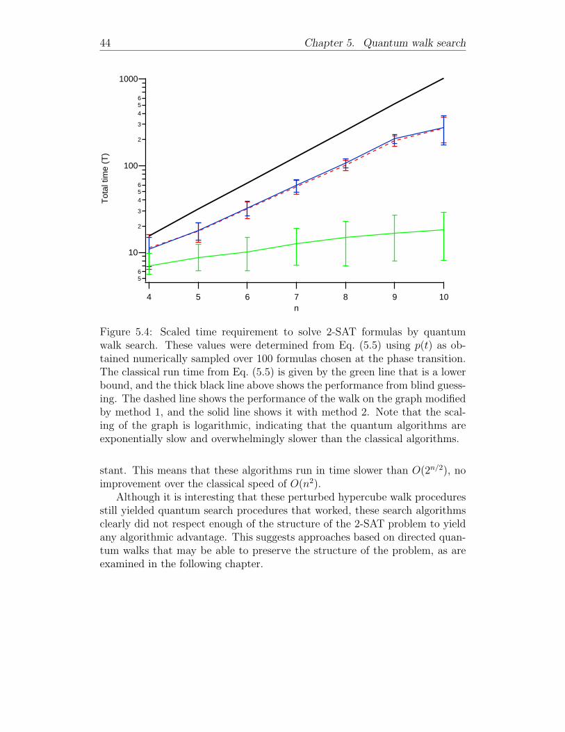
44 Chapter 5. Quantum walk search
56
10
2
3
456
100
2
3
456
1000
Tot
al ti
me
(T)
10987654n
Figure 5.4: Scaled time requirement to solve 2-SAT formulas by quantumwalk search. These values were determined from Eq. (5.5) using p(t) as ob-tained numerically sampled over 100 formulas chosen at the phase transition.The classical run time from Eq. (5.5) is given by the green line that is a lowerbound, and the thick black line above shows the performance from blind guess-ing. The dashed line shows the performance of the walk on the graph modifiedby method 1, and the solid line shows it with method 2. Note that the scal-ing of the graph is logarithmic, indicating that the quantum algorithms areexponentially slow and overwhelmingly slower than the classical algorithms.
stant. This means that these algorithms run in time slower than O(2n/2), noimprovement over the classical speed of O(n2).
Although it is interesting that these perturbed hypercube walk proceduresstill yielded quantum search procedures that worked, these search algorithmsclearly did not respect enough of the structure of the 2-SAT problem to yieldany algorithmic advantage. This suggests approaches based on directed quan-tum walks that may be able to preserve the structure of the problem, as areexamined in the following chapter.

5.5. Quantum search on 2-SAT 45
500
400
300
200
100
0
Min
imal
tota
l tim
e (T
)
2520151050Number of solutions
Figure 5.5: Minimal time required to solve 2-SAT formulas by quantum walksearch vs. the number of satisfying truth assignments. The size of each dia-mond indicates the multiplicity at each point. These values were determinedfrom Eq. (5.5) directly for each individual formula, and were taken from thedata used to generated Fig. 5.4 with n = 10, so these formulas were at thephase transition. This plot clearly shows a strong correlation exactly oppositethat of the classical algorithm: the presence of additional solutions makes thealgorithm slower. Since these SAT formulas were also randomly generated atthe phase transition, it shows that in general we cannot expect these formulasto only have a few solutions.
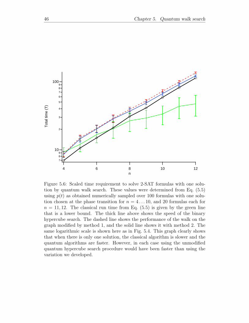
46 Chapter 5. Quantum walk search
7
89
10
2
3
4
5
6
7
89
100
Tot
al ti
me
(T)
1210864n
Figure 5.6: Scaled time requirement to solve 2-SAT formulas with one solu-tion by quantum walk search. These values were determined from Eq. (5.5)using p(t) as obtained numerically sampled over 100 formulas with one solu-tion chosen at the phase transition for n = 4 . . . 10, and 20 formulas each forn = 11, 12. The classical run time from Eq. (5.5) is given by the green linethat is a lower bound. The thick line above shows the speed of the binaryhypercube search. The dashed line shows the performance of the walk on thegraph modified by method 1, and the solid line shows it with method 2. Thesame logarithmic scale is shown here as in Fig. 5.4. This graph clearly showsthat when there is only one solution, the classical algorithm is slower and thequantum algorithms are faster. However, in each case using the unmodifiedquantum hypercube search procedure would have been faster than using thevariation we developed.
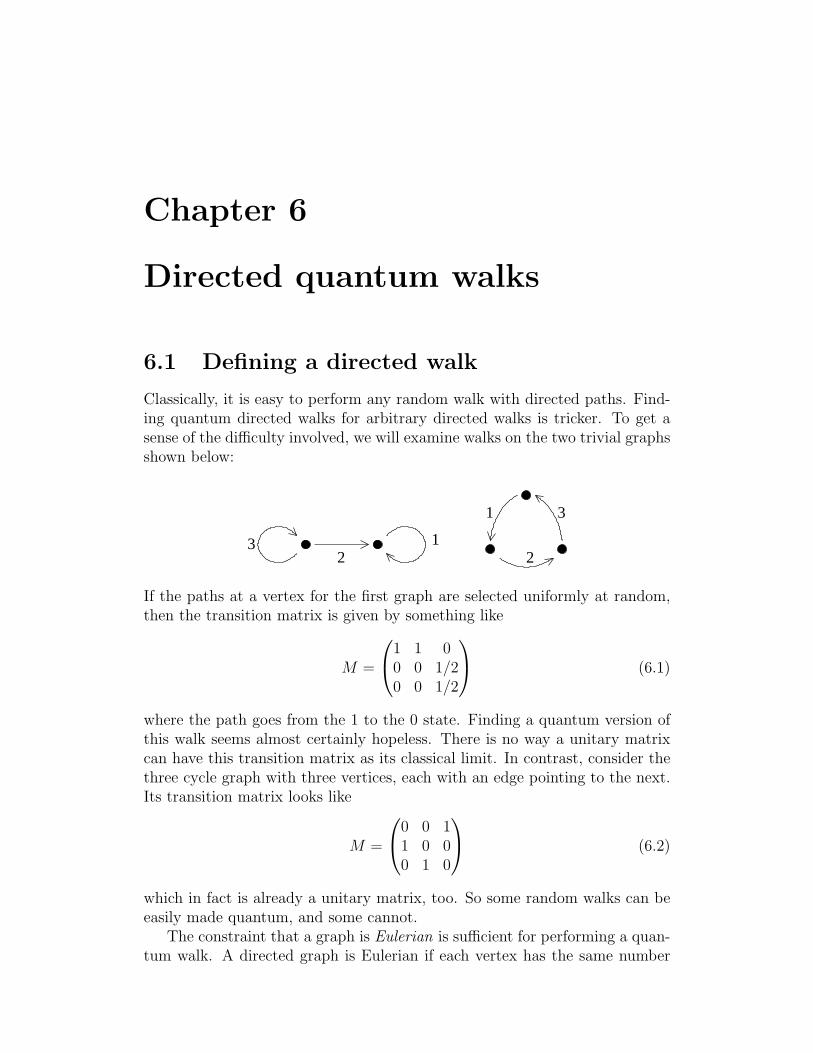
Chapter 6
Directed quantum walks
6.1 Defining a directed walk
Classically, it is easy to perform any random walk with directed paths. Find-ing quantum directed walks for arbitrary directed walks is tricker. To get asense of the difficulty involved, we will examine walks on the two trivial graphsshown below:
3 12
3
2
1
If the paths at a vertex for the first graph are selected uniformly at random,then the transition matrix is given by something like
M =
1 1 00 0 1/20 0 1/2
(6.1)
where the path goes from the 1 to the 0 state. Finding a quantum version ofthis walk seems almost certainly hopeless. There is no way a unitary matrixcan have this transition matrix as its classical limit. In contrast, consider thethree cycle graph with three vertices, each with an edge pointing to the next.Its transition matrix looks like
M =
0 0 11 0 00 1 0
(6.2)
which in fact is already a unitary matrix, too. So some random walks can beeasily made quantum, and some cannot.
The constraint that a graph is Eulerian is sufficient for performing a quan-tum walk. A directed graph is Eulerian if each vertex has the same number
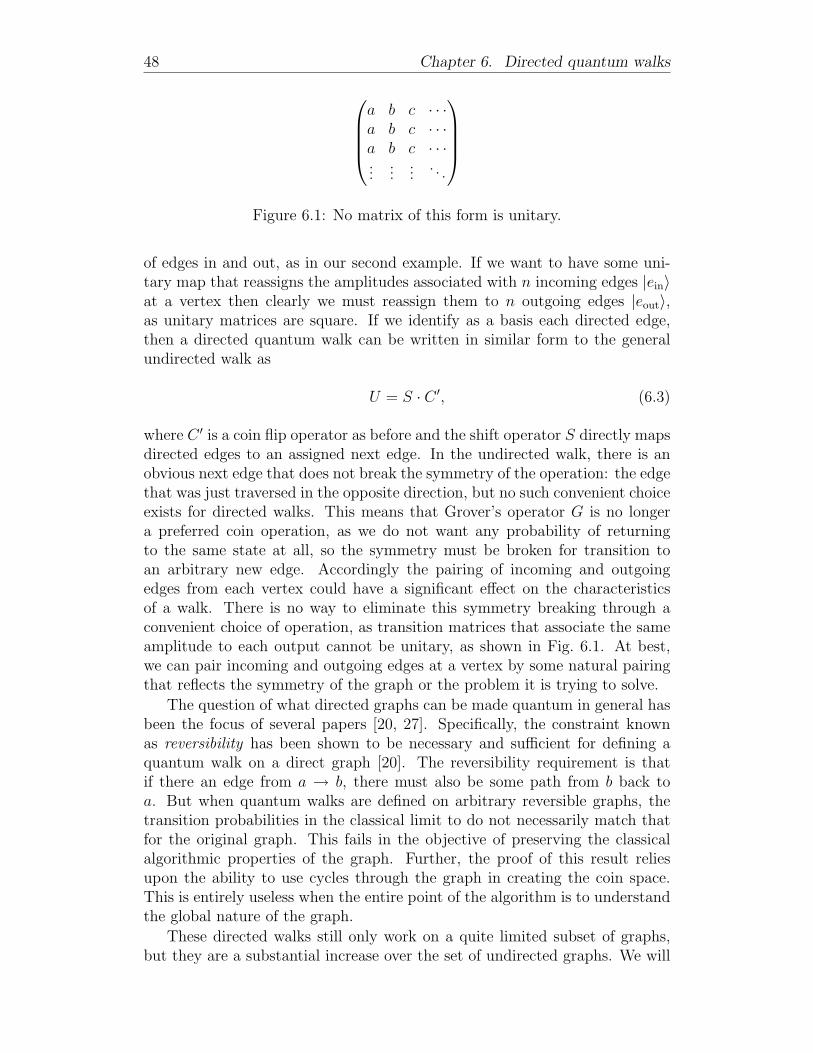
48 Chapter 6. Directed quantum walks
a b c · · ·a b c · · ·a b c · · ·...
......
. . .
Figure 6.1: No matrix of this form is unitary.
of edges in and out, as in our second example. If we want to have some uni-tary map that reassigns the amplitudes associated with n incoming edges |ein〉at a vertex then clearly we must reassign them to n outgoing edges |eout〉,as unitary matrices are square. If we identify as a basis each directed edge,then a directed quantum walk can be written in similar form to the generalundirected walk as
U = S · C ′, (6.3)
where C ′ is a coin flip operator as before and the shift operator S directly mapsdirected edges to an assigned next edge. In the undirected walk, there is anobvious next edge that does not break the symmetry of the operation: the edgethat was just traversed in the opposite direction, but no such convenient choiceexists for directed walks. This means that Grover’s operator G is no longera preferred coin operation, as we do not want any probability of returningto the same state at all, so the symmetry must be broken for transition toan arbitrary new edge. Accordingly the pairing of incoming and outgoingedges from each vertex could have a significant effect on the characteristicsof a walk. There is no way to eliminate this symmetry breaking through aconvenient choice of operation, as transition matrices that associate the sameamplitude to each output cannot be unitary, as shown in Fig. 6.1. At best,we can pair incoming and outgoing edges at a vertex by some natural pairingthat reflects the symmetry of the graph or the problem it is trying to solve.
The question of what directed graphs can be made quantum in general hasbeen the focus of several papers [20, 27]. Specifically, the constraint knownas reversibility has been shown to be necessary and sufficient for defining aquantum walk on a direct graph [20]. The reversibility requirement is thatif there an edge from a → b, there must also be some path from b back toa. But when quantum walks are defined on arbitrary reversible graphs, thetransition probabilities in the classical limit to do not necessarily match thatfor the original graph. This fails in the objective of preserving the classicalalgorithmic properties of the graph. Further, the proof of this result reliesupon the ability to use cycles through the graph in creating the coin space.This is entirely useless when the entire point of the algorithm is to understandthe global nature of the graph.
These directed walks still only work on a quite limited subset of graphs,but they are a substantial increase over the set of undirected graphs. We will
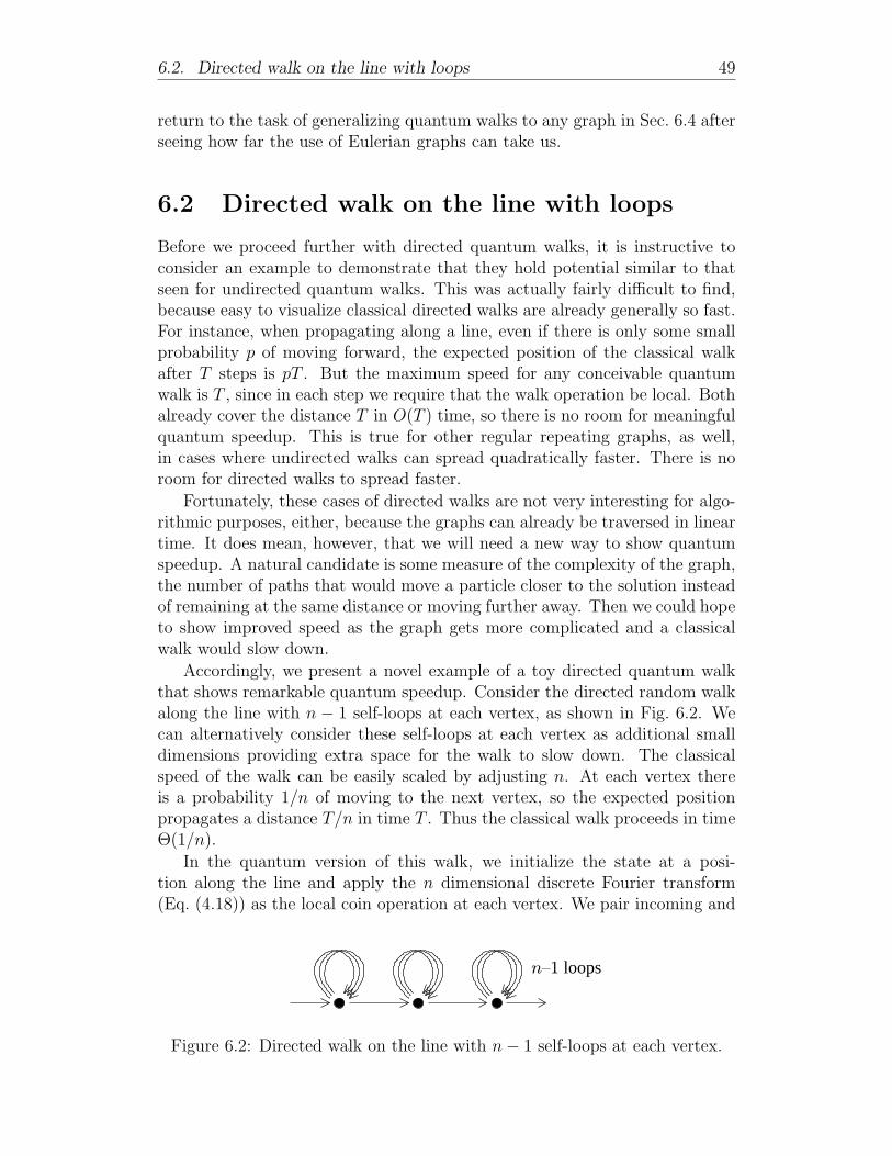
6.2. Directed walk on the line with loops 49
return to the task of generalizing quantum walks to any graph in Sec. 6.4 afterseeing how far the use of Eulerian graphs can take us.
6.2 Directed walk on the line with loops
Before we proceed further with directed quantum walks, it is instructive toconsider an example to demonstrate that they hold potential similar to thatseen for undirected quantum walks. This was actually fairly difficult to find,because easy to visualize classical directed walks are already generally so fast.For instance, when propagating along a line, even if there is only some smallprobability p of moving forward, the expected position of the classical walkafter T steps is pT . But the maximum speed for any conceivable quantumwalk is T , since in each step we require that the walk operation be local. Bothalready cover the distance T in O(T ) time, so there is no room for meaningfulquantum speedup. This is true for other regular repeating graphs, as well,in cases where undirected walks can spread quadratically faster. There is noroom for directed walks to spread faster.
Fortunately, these cases of directed walks are not very interesting for algo-rithmic purposes, either, because the graphs can already be traversed in lineartime. It does mean, however, that we will need a new way to show quantumspeedup. A natural candidate is some measure of the complexity of the graph,the number of paths that would move a particle closer to the solution insteadof remaining at the same distance or moving further away. Then we could hopeto show improved speed as the graph gets more complicated and a classicalwalk would slow down.
Accordingly, we present a novel example of a toy directed quantum walkthat shows remarkable quantum speedup. Consider the directed random walkalong the line with n − 1 self-loops at each vertex, as shown in Fig. 6.2. Wecan alternatively consider these self-loops at each vertex as additional smalldimensions providing extra space for the walk to slow down. The classicalspeed of the walk can be easily scaled by adjusting n. At each vertex thereis a probability 1/n of moving to the next vertex, so the expected positionpropagates a distance T/n in time T . Thus the classical walk proceeds in timeΘ(1/n).
In the quantum version of this walk, we initialize the state at a posi-tion along the line and apply the n dimensional discrete Fourier transform(Eq. (4.18)) as the local coin operation at each vertex. We pair incoming and
loops1n
Figure 6.2: Directed walk on the line with n− 1 self-loops at each vertex.

50 Chapter 6. Directed quantum walks
50x10-3
40
30
20
10
0
p
5004003002001000x
n=2
n=5
n=10
n=2n=5n=10
Figure 6.3: Classical vs. quantum directed walks with loops after 500 timesteps, for increasing number of loops n. The classical walks are those with theGaussian shape and the quantum walks are those exhibiting the characteris-tic interference pattern. The classical proceed on average a distance 500/n,whereas the quantum walks converge to proceeding a constant distance.
outgoing edges in the only non-symmetry breaking manner, by associating self-loops with themselves and pairing the incoming and outgoing paths along theline. Starting in a definite state at one edge along the line, numerical resultsshow that as n → ∞, the expected position of this walk propagates T stepsforward in time T/2, independent of n. This is in time Θ(1). Superimposedpictures of the walk after 100 steps for increasing n are shown in Fig. 6.3. Thespeed of the walk over time is shown in Fig. 6.4 clearly converging to 1/2 stepforward per time step. The speed of this walk has been verified numericallyfor up to n = 1000.
This walk proceeds quickly by strongly exploiting the symmetry of itssetup. We can understand how it works by considering the effects of thediscrete Fourier transform in two steps. Starting with the |0〉 state, it is trans-formed to the equal superposition
|ψ〉 =1√n
(|0〉+ |1〉+ . . .+ |n− 1〉).
The inverse discrete Fourier transform is given by
|j〉 → 1√n
n−1∑k=0
e−2πijk/n |k〉 , (6.4)
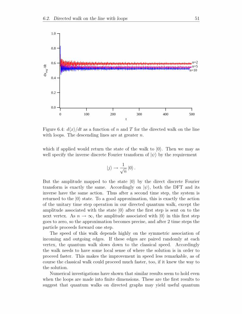
6.2. Directed walk on the line with loops 51
1.0
0.8
0.6
0.4
0.2
0.0
dxax
g /d
t
5004003002001000t
n=2n=5
n=10
Figure 6.4: d〈x〉/dt as a function of n and T for the directed walk on the linewith loops. The descending lines are at greater n.
which if applied would return the state of the walk to |0〉. Then we may aswell specify the inverse discrete Fourier transform of |ψ〉 by the requirement
|j〉 → 1√n|0〉 .
But the amplitude mapped to the state |0〉 by the direct discrete Fouriertransform is exactly the same. Accordingly on |ψ〉, both the DFT and itsinverse have the same action. Thus after a second time step, the system isreturned to the |0〉 state. To a good approximation, this is exactly the actionof the unitary time step operation in our directed quantum walk, except theamplitude associated with the state |0〉 after the first step is sent on to thenext vertex. As n → ∞, the amplitude associated with |0〉 in this first stepgoes to zero, so the approximation becomes precise, and after 2 time steps theparticle proceeds forward one step.
The speed of this walk depends highly on the symmetric association ofincoming and outgoing edges. If these edges are paired randomly at eachvertex, the quantum walk slows down to the classical speed. Accordinglythe walk needs to have some local sense of where the solution is in order toproceed faster. This makes the improvement in speed less remarkable, as ofcourse the classical walk could proceed much faster, too, if it knew the way tothe solution.
Numerical investigations have shown that similar results seem to hold evenwhen the loops are made into finite dimensions. These are the first results tosuggest that quantum walks on directed graphs may yield useful quantum
52 Chapter 6. Directed quantum walks
algorithms, and suggest that this approach may have merit, although thespeedup we have found is different and perhaps harder to obtain than thatwith undirected quantum walks.
6.3 Returning to k-SAT
Of course, the graphs from k-SAT problems are not necessarily Eulerian, sowe cannot yet run a directed walk on them. Reflecting the difficulty of SAT,there are no nice restrictions on the number of edges in and out of each ver-tex on graphs corresponding to SAT formulas. Along the lines developed inChapter 5, a natural first thought is to create some sort of edge Oracle thatconditionally fixes the graph by adding in additional directed edges as neces-sary to make them Eulerian. But such a procedure is not helpful here, becauseadding edges to fix the graph at each vertex simultaneously would not fix thegraph in one step. The fix of adding an new edge to or away from one vertexwould throw off the count of in and out edges at the adjacent vertex. Anyquantum walk search algorithm needs to be local, as querying the entire graphto fix it up is equivalent to solving the problem directly. Even worse, there isno way for probability to build up at solutions if there are paths leaving them,so the idea of conserving the number of paths in and out of every vertex isdoomed at those vertices representing solutions. With this conundrum, we areleft to consider the options for non-unitary quantum walk operations.
6.4 General quantum operations
Recall that the statistical ensemble of state vectors |ψi〉 with probabilities piis described by a density operator ρ given by
ρ =∑i
pi |ψi〉〈ψi| . (6.5)
An ensemble of density operators ρi with probabilities pi is given by∑
i piρi.Density operators in general are the set of positive semi-definite matrices withtrace 1. Pure states are the set of density operator that can be representedexactly as a single state vector |ψ〉, that is, if a density operator has onenon-zero eigenvalue. States that are not pure are called mixed and representclassical ensembles of pure states. We evolve the state ρ by an operation E inthe usual fashion by the use of a unitary operator U such that
E(ρ) = UρU †. (6.6)
These unitary operators classify the full range of quantum transitions in closedsystems without measurement.
But this is not the full range of manners in which one quantum state maybe mapped onto another. Consider a quantum black box that maps arbitrary
6.4. General quantum operations 53
quantum systems using physical processes. Inside, it can store any sort ofancillary quantum systems, to which we can apply a joint operation with oursystem of interest. The black box lets out another quantum system, but it mustnot necessarily even have the same size as the original system. For example,it could take two qubits as input and throw away one, only outputting theremaining qubit. It turns out that in general we can express any such blackbox E , termed a general quantum operation or super operator, as
E(ρ) =∑i
EiρE†i , (6.7)
where Ei is any set of complex matrices satisfying∑i
E†iEi ≤ I, (6.8)
where the ≤ sign indicates that I −∑
iE†iEi must be a positive-semidefinite
operator. For an operator from an n dimensional state to an m dimensionalstate, only at most mn operator elements Ei are needed to describe it. Also,just as a combination of pure states is not uniquely specified by a densityoperator, a set of operator elements is not uniquely specified by an quantumoperation.
This formalism is most commonly used to rigorously describe the phe-nomena of decoherence, as quantum systems become classical due to noise.Using non-unitary operators E in quantum algorithms does not give space fornew quantum phenomena, but allows us to make algorithms more classical ina controlled and limited way. This suggests a strategy for extending directedquantum walks to general graphs in a manner in which they may still maintainsome of their quantum properties.
It can be shown that Eq. (6.7) and (6.8) are a complete classification of alloperators arising from the restrictions imposed by the following set of physicalprinciples [23]:
1. Tr E(ρ) ≤ 1, where the equality is strict unless the process is explicitlydependent upon the results of measurement. This inequality correspondsto the inequality in Eq. (6.8).
2. Applying the operation separately to a set of quantum states which arethen mixed together should be equivalent to applying the operation tothe states combined first:
E
(∑i
piρi
)=∑i
piE(ρi). (6.9)
3. If we consider ρ as part of any other quantum state described by a densityoperator, the final state should still be a density operator. This meansthat the operator I ⊗ E should also map density operators to densityoperators, where I is the identity operator on any finite size space.

54 Chapter 6. Directed quantum walks
ρn
U
mE(ρ)
|0〉〈0|m2 mn
discarded
Figure 6.5: General quantum operations as unitary evolution of the system ofinterest and an environmental system. The numbers above the lines indicatethe dimensionality of the quantum systems being manipulated.
When not dependent upon measurement results, these operators can alsobe described by a unitary operator acting on the combined system. Given ageneral quantum operation E , we can describe its action by a unitary matrix Uacting on ρ⊗|0〉〈0|, where |0〉〈0| is a label associated with some environmentalsystem in its initial state, and then discarding all but some m dimensionalstate. We can explicitly write U acting on the pure state |0〉 ⊗ |ψ〉 as
U =
[E1] . . .[E2] . . .
... . . .[Emn] . . .
, (6.10)
where the Ei are a set of operator element corresponding to the operator andall but the first block column is filled in arbitrarily to make the matrix uni-tary. Each operator Ei corresponds to a particular basis state |ei〉 in the finalenvironmental system. Then discarding this environment corresponds to mea-suring all states by |ei〉, obtaining the states 1√
piEi |ψ〉 each with probability
pi = 〈ψ|E†iEi |ψ〉. Schematically, this corresponds to the quantum circuitshown in Fig. 6.5. Since the density matrix for this new state is∑
i
Ei |ψ〉〈ψ|E†i , (6.11)
and we can write any density matrix as a sum of pure states, this procedurecorresponds exactly to the operation E .
This picture of general quantum operations is significant for two reasons.First of all, it shows that they can be specified by a unitary operation andadding only at most a certain number of temporary ancillary qubits. Itdemonstrates that in principle using such a general operation instead of aunitary transformation does not increase the permanent spatial requirementsof a quantum algorithm and nor change the order of its run time.
Secondly, this result establishes shows that we can classically simulatequantum algorithms involving general quantum operations without revert-ing to the density matrix formalism. Simulating a quantum system in thedensity matrix formalism instead of with state vectors increases the memoryrequirements by a quadratic factor and increases the calculation requirementsjust as much. The simulation requirements to exactly calculate transitions of
6.5. Directed quantum walks on any graph 55
general quantum operators with density matrices could be even worse, sinceunlike unitary operators acting on independent subspaces, general quantumoperations cannot be easily separated. Accordingly applying non-trivial gen-eral operations to density operators would involve exponentially larger matrixmultiplication when simulating systems like quantum walks. By using quan-tum Monte-Carlo simulation with state vectors, we can model these algorithmsfar faster than from exact evaluation using density operators.
6.5 Directed quantum walks on any graph
We can now can write a quantum walk for any directed graph. Writing a singlestep of the walk as the composition of a shift and coin operation again, wehave
U = S ′ C ′, (6.12)
where U is no longer necessarily unitary. The coin C ′ is of the form for generalundirected graphs, but the shift S ′ must incorporates possibly changing the sizeof the spaces at each vertices, and thus must include some non-trivial generalquantum operation. It also includes an explicit step pairing the possibly sizechanged amplitudes at a vertex with outgoing edges. In general, we can breakdown S ′ into the direct sum of shifts that happen at each vertex. At eachvertex, there are n edges in and m edges out, leaving three possible cases. Ifn = m, then we can apply straightforward permutation, a unitary operation.If n < m, then we can also apply permutation, by classically choosing thevertices to be shifted onto at random. The hard case is for n > m, becausethen we need to somehow over-compress quantum states onto a smaller space.In general, we know this is not possible with perfect fidelity for arbitrary purestates, because quantum operations must be linear, and there are no invertiblelinear maps from a space of higher to lower dimensionality. At best, we canhope to compress the state in such a way that only some minimal amount ofinformation is lost.
We now consider such choices of “over-compressing” operations in the casethat there are more paths in n than out m. One of the easiest such operatorsto devise is to create an equal classical superposition of all outgoing stateseach time it is applied. This operation has operator elements given by
Eij =1√m|j〉〈i| . (6.13)
where 1 ≤ i ≤ n and 1 ≤ j ≤ m. We can easily verify
∑i,j
E†ijEij =1
m
∑i,j
|i〉〈j|j〉〈i| =n∑i=1
|i〉〈i| = I, (6.14)
56 Chapter 6. Directed quantum walks
as required by Eq. (6.8). Then its action on a state ρ is given by∑i,j
EijρE†ij =
1
m
∑i,j
|j〉〈i|ρ|i〉〈j| (6.15)
=1
m
n∑i=1
〈i|ρ|i〉m∑j=1
|j〉〈j| (6.16)
=1
mTr(ρ)I (6.17)
= I/m, (6.18)
which is exactly the classical superposition of the states |j〉 with probability1/m each. But classical superpositions do not provide room for quantuminterference, so this is a poor candidate for our shift operation.
A more sophisticated transition operator picks m input states at randomand maps them to output states, discarding n − m states. This operator isgiven by operator elements
Ei =1√mn
(nm
) m∑j=1
|j〉〈ij| , (6.19)
where |ij〉 indicates the jth basis vector from the ith choice of m out of n basisvectors for the input space. We can verify
∑i∈C
E†iEi =n/m(nm
) ∑i∈C
m∑j=1
|ij〉〈j|j〉〈ij| =n/m(nm
) ∑i∈C
m∑j=1
|ij〉〈ij| = I, (6.20)
where C is the set of m choices of n, as on average each sum∑m
j=1 |ij〉〈ij|contributes m
nI and there are
(nm
)choices, so this is a general quantum opera-
tion. To get some limited sense of how this operator acts, consider its actionreducing an arbitrary state in 3 dimensions to 2 dimensions,a b c
e f gh j k
→ (a+ 1
2f 1
2(b+ c+ g)
12(e+ h+ j) 1
2f + k
). (6.21)
In some sense the matrix elements of this resulting state look similar to theoriginal. More broadly, it is hard to understand what this operator does, butat least its transitions clearly remain significantly quantum mechanical.
6.6 Quantum directed walks on 2-SAT
In the full procedure, we start the directed quantum walk in an initial stateat an equal superposition of being at each vertex. Then we use a standardcoin operator C ′ and a shift operator including one of the over-compression

6.7. Conclusions 57
operators as given by Eq. (6.13) or Eq. (6.19). As we have no heuristic to pairin and out edges at any vertex, we resort choosing random pairings with theshift operation.
Unfortunately, when averaged over a sufficiently large number of runs,numerical results show that the average probability of any quantum walk con-verging to a solution after running the walk for any time t is exactly equalto the probability from simulating the classical walk with a Markov chain.Although the first transition operator is almost entirely useless, keeping thepairing between in and out edges at some random constant assignment overthe course of quantum walk yields varied results at least for the second opera-tor. But on average for every 2-SAT formula the performance of the classicaland quantum walks are identically the same. By pairing in and out verticesrandomly, we seem to have averaged over all quantum interference effects suchthat they are entirely unnoticeable.
6.7 Conclusions
Quantum random walks provide a simple model of quantum systems that em-phasize the profound power of quantum interference. Constructive interferenceallows probability to build up faster in quantum walks than can be done clas-sically. Intuitively, it is clear that in order for interference to build up in amanner that reflects the symmetry of a particular problem, the quantum walkitself must as much as possible reflect that symmetry. The examples of quan-tum walks we have discussed that are successfully faster than their classicalversions respect most of the symmetry of the underlying graph obtained fromthe classical version, and this is an observation also consistent more generallywith the most powerful quantum walks [18]. Our failure to find a way to re-spect symmetry when approaching SAT with directed quantum walks explainswhy these algorithms were not successful.
In our work with directed walks, we may also have been moving too fast inour attempts to solve satisfiability problems. We provided the first demonstra-tion of the power of directed quantum walks (Sec. 6.2) and then immediatelyattempted to solve the very hard problem of satisfiability. Careful intermedi-ate work would warranted, using directed quantum walks to solve more toyproblems with intrinsically more accessible symmetry. A good starting pointfor further investigations would be to attempt to find more examples of use-ful quantum versions of directed walks on the hypercube or other structureswith similarities to the graphs used in satisfiability problems, in a manner thatis not as ambitious as attacking SAT directly. As it turns out, satisfiabilityproblems may simply not have sufficient symmetry to be exploited by quan-tum walks, but further investigations toward these conclusions could still yieldother useful insights.
In fact, hoping to spur these other insights was always the primary moti-vation for this work, as ironically a quantum algorithm for 3-SAT better than
58 Chapter 6. Directed quantum walks
any classical algorithm already exists. It is essentially the best probabilisticalgorithm for 3-SAT plugged directly into Grover’s algorithm, which can makeany algorithm that succeeds with bounded probability run in the square rootof the time [6]. One might wonder in that case why we even looked for animprovement that could be expected at best to only match that performance,but even solving 3-SAT is only relevant because of its connection to a biggerclasses of problems. The most important aspect of this work is the guidanceit yields toward future quantum random walk based algorithms for problemsthat may not have such easy shortcuts, and, in a pinch, that guidance couldbe summarized in one word and essential concept: symmetry.
Acknowledgments
First and foremost, I would like to thank my research adviser last summer,David Meyer, under whom I performed most of this research. He introducedme to quantum computing and quantum walks, and was extremely helpful inguiding my research and providing feedback on this thesis.
I had a tremendously fun summer doing physics at UCSD thanks to mycompanions in the REU program. The comments and feedback from the fellowstudents in David’s group were also hugely helpful, especially from Yi-Kai Liuwho gave me some useful pointers on satisfiability problems. I would also liketo thank my friend Eric Christiansen for convincing me to program in Pythonand for his (futile) attempts to understand quantum mechanics.
I am indebted to the UCSD Mathematics department Computing Support,which lent me a laptop when my own was stolen three weeks before the endof my work. For that matter, I can also thank the coincidence that I backedup all my work to a server only two days before.
Finally, I am grateful to my thesis readers at Swarthmore, John Boccioand Amy Bug, for reading this thesis with a critical eye even though it wasoutside their specialty, and also the entire physics department at Swarthmorefor giving me a fantastic education.
This research was funded mostly by the NSF under the 2007 REU programat the University of California San Diego.

References
[1] Scott Aaronson. The limits of quantum computers. Scientific American,298(3):62, Mar 2008.
[2] Scott Aaronson and Andris Ambainis. Quantum search of spatial regions.In FOCS ’03: Proceedings of the 44th Annual IEEE Symposium on theFoundations of Computer Science, page 200, 2003.
[3] Dorit Aharonov, Andris Ambainis, Julia Kempe, and Umesh Vazirani.Quantum walks on graphs. In STOC ’01: Proceedings of the 33rd An-nual ACM Symposium on Theory of Computing, pages 50–59, July 2001,arXiv:quant-ph/0012090.
[4] Y. Aharonov, L. Davidovich, and N. Zagury. Quantum random walks.Phys. Rev. A, 48(2):1687–1690, Aug 1993.
[5] Andris Ambainis. Quantum walks and their algorithmic applica-tions. International Journal of Quantum Information, 1:507–518, 2003,arXiv:quant-ph/0403120.
[6] Andris Ambainis. Quantum search algorithms. SIGACT News, 35(2):22–35, 2004, arXiv:quant-ph/0504012.
[7] Andris Ambainis, Eric Bach, Ashwin Nayak, Ashvin Vishwanath, andJohn Watrous. One-dimensional quantum walks. In STOC ’01: Proceed-ings of the 33rd Annual ACM Symposium on Theory of Computing, pages37–49, New York, NY, USA, 2001.
[8] Paul Benioff. Space searches with a quantum robot. AMS ContemporaryMath Series, Vol, 305, 2002, arXiv:quant-ph/0003006.
[9] Bla Bollobs, Christian Borgs, Jennifer T. Chayes, Jeong Han Kim, andDavid B. Wilson. The scaling window of the 2-SAT transition. RandomStructures and Algorithms, 18(3):201–256, 2001, arXiv:math/9909031.
[10] Andrew M. Childs, Richard Cleve, Enrico Deotto, Edward Farhi, SamGutmann, and Daniel A. Spielman. Exponential algorithmic speedupby quantum walk. In STOC ’03: Proceedings of the 35th Annual ACMSymposium on Theory of Computing, pages 59–68, 2003, arXiv:quant-ph/0209131.
62 References
[11] Andrew M. Childs and Jeffrey Goldstone. Spatial search by quantumwalk. Phys. Rev. A, 70:022314, 2004, arXiv:quant-ph/0306054.
[12] D. Deutch. Quantum theory, the Church-Turing principle and the uni-versal quantum computer. In Proceedings of the Royal Society of London,volume 400 of A, Mathematical and Physical Sciences, pages 97–117, 1985.
[13] Richard P. Feynman. Simulating physics with computers. InternationalJournal of Thoeretical Physics, 21(6/7):467–488, Jun 1982.
[14] Lov K. Grover. A fast quantum mechanical algorithm for databasesearch. In STOC ’96: Proceedings of the 28th annual ACM Symposiumon the Theory of Computing, pages 212–219, May 1996, arXiv:quant-ph/9605043.
[15] Tad Hogg. Solving random satisfiability problems with quantum comput-ers. 2001, arXiv:quant-ph/0104048.
[16] Julia Kempe. Quantum random walks - an introductory overview. Con-temporary Physics, 44(4):307–327, 2003, arXiv:quant-ph/0303081.
[17] Viv Kendon. Decoherence in quantum walks - a review. MathematicalStructures in Computer Science, 17(6):1169–1220, Dec 2007, arXiv:quant-ph/0606016.
[18] Hari Krovi and Todd A. Brun. Hitting time for quantum walks on thehypercube. Phys. Rev. A, 73:032341, 2006, arXiv:quant-ph/0510136.
[19] David A. Meyer. From quantum cellular automata to quantum latticegases. J. Stat. Phys., 85:551–574, 1996, arXiv:quant-ph/9604003.
[20] Ashley Montanaro. Quantum walks on directed graphs. Quantum Infor-mation and Computation, 7(1), 2007, arXiv:quant-ph/0504116.
[21] Cristopher Moore and Alexander Russell. Quantum walks on the hyper-cube. In RANDOM ’02: Proceedings of the 6th International Workshopon Randomization and Approximation Techniques, pages 164–178, Lon-don, UK, 2002. Springer-Verlag, arXiv:quant-ph/0104137.
[22] Rajeev Motwani and Prabhakar Raghavan. Randomized Algorithms.Cambridge University Press, Cambridge, UK, 1995.
[23] Michael A. Nielsen and Isaac L. Chaung. Quantum Computation andQuantum Information. Cambridge University Press, Cambridge, UK,2000.
[24] C.H. Papadimitriou. On selecting a satisfying truth assignment. In FOCS’91: Proceedings of the 32nd Annual IEEE Symposium on the Foundationsof Computer Science, pages 163–169, October 1991.
References 63
[25] Robin Pemantle, Rajarshi Das, and Torin Greenwood. Quantum ran-dom walks archive. Available online at http://www.math.upenn.edu/
~pemantle/Summer2007/Archive.html, Aug 2007.
[26] Uwe Schoning. A probabilistic algorithm for k-SAT and constraint sat-isfaction problems. In FOCS ’99: Proceedings of the 40th Annual IEEESymposium on the Foundations of Computer Science, pages 410–414, Oc-tober 1999.
[27] Simone Severini. On the digraph of a unitary matrix. SIAM J. MatrixAnal. Appl., 25(1):295–300, 2003, arXiv:math/0205187.
[28] Neil Shenvi, Julia Kempe, and K. Birgitta Whaley. Quantum random-walk search algorithm. Phys. Rev. A, 67(5):052307, May 2003,arXiv:quant-ph/0210064.
[29] Peter W. Shor. Polynomial-time algorithms for prime factorization anddiscrete logarithms on a quantum computer. In FOCS ’94: Proceedingsof the 35th Annual IEEE Symposium the on Foundations of ComputerScience, pages 124–134, 1994, arXiv:quant-ph/9508027.