Quantum Monte Carlo calculations on Rydberg states … · QMC workshop, The Towler Institute, ... Importance sampled DMC algorithm: ... node optimization for rydberg states 1P

Quantum Monte Carlo calculations onRydberg states and transition metal

oxides

Arne Lüchow , Tony C. Scott, and Annika Bande

Theoretical chemistryInstitute of physical chemistry

RWTH Aachen university

QMC workshop, The Towler Institute, July 26 - August 2, 2008

– p.1/41

Outline

Few details of our quantum Monte Carlo methods

Excited states: nodal domains

Optimal nodes in fixed-node DMC

vanadium oxides with QMC

– p.2/41

DMC: Importance Sampling with Guide Function

guide function ΦG(r) forces spatial and spin symmetry

f(r, τ) := Ψ(r, τ)ΦG(r)

Hamiltonian H = ΦGHΦ−1

G− Eref (non-Hermitian)

Importance sampled DMC algorithm:

diffusion step

drift step towards large |ΦG(r)|weight/branch step with e

−(EL(r)−Eref)τ

with local energy: EL(r) =HΦG(r)

ΦG(r)

ΦG can statisfy (two-particle) cusp conditions⇒ singularities vanish!

Asymptotic (τ →∞) probability density f(r, τ)→ ΦG(r)Φ0(r)

– p.3/41

Quantum Monte Carlo for Electron Structure

Pauli principle causes nodes in wave function: Ψ(r) = 0

Fermion sign problem!

example: exact nodes for 3S He: r1 = r2

Ψ(r1, r1, r12) = −Ψ(r1, r1, r12)⇒ Ψ = 0

note: orbital ansatz Ψ = 1s12s1 has exact nodes,no correlation effect on nodes: complicated wf but simple nodes!

more exact nodes: Lubos Mitas and coworker

– p.4/41

exact Helium nodes

Similar for singlet states 1S He?

Is there a correlation effect on nodes, i.e. dependence on r12 or θ12?

High accuracy Hylleraas-CI wavefunctions indicate:no dependence on θ12 (Bressanini, Reynolds)

We find with very high accuracy (Frankowski-Pekeris basis):

Small but significant dependence on θ12:simple nodes, very weak correlation dependence

0

0.5

1

1.5

2

0 0.5 1 1.5 2

r 2 (

bohr

)

r1 (bohr)

1.367

1.368

1.369

1.37

1.371

1.372

1.373

1.374

1.375

0 0.5 1 1.5 2 2.5 3

r 1 =

r2 (b

ohr)

θ12

a T.C. Scott, A. Lüchow, D. Bressanini, J.D. Morgan III, PRA 75,060101(R), (2007) – p.5/41

Quantum Monte Carlo for Electron Structure

nodes are 3n− 1-dimensional hypersurfaces

fixed node approximation (FN-DMC):use nodes from known functions (here: ab initio)

usually: enforce nodes from guide function ΦG = ΦdeteU then

Ψ(τ)ΦG ≥ 0 (probability density)

FN-DMC solves Schrödinger equation with additional boundarycondition exactly

→ node location error

or: released-node methods

– p.6/41

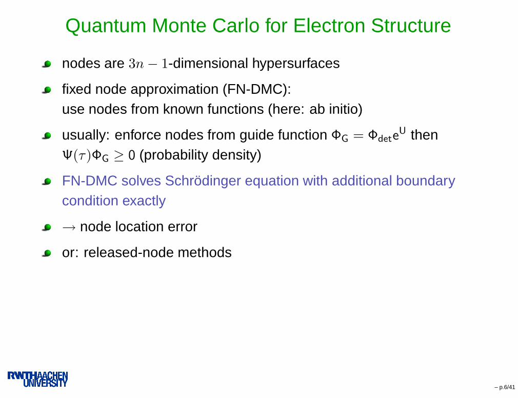
excited states with DMC: nodal domains

consequences of the fixed-node approximation:

3n− 1 dimensional nodal hypersurface partitions the space R3n

in disjoint domains ΩjFN-DMC means: Solving S.E. in one or more domains

HΨ(j)0 (r) = E

(j)0 Ψ

(j)0 (r) for r ∈ Ωj

Ψ(j)0 (r) = 0 for r 6∈ Ωj

domain energies E(j)0 are identical if domains Ωj are related by

permutation

Tiling theorem (Ceperley): in exact ground state all domains arerelated by permutation

spurious nodes: even in ground state e.g. through limited basisa

excitation nodes: different domains Ωj in excited states

a J. Hachmann et al. (Handy group) CPL 392, 55 (2004)– p.7/41

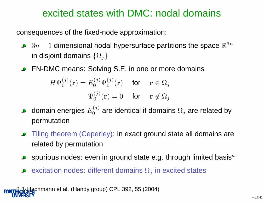
Rydberg states with QMC

generally:

the higher the excitation the more hydrogenic the Rydberg orbitalbecomes, even for molecules

HF or standard DFT virtual orbitals too diffuse

excited state calculations with QMC require guide functions withmany Slater determinants

CASSCF-type calculations do not scale well and result in manydeterminants

– p.8/41

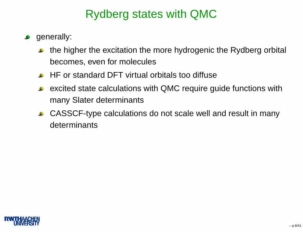
Rydberg states with QMC

generally:

the higher the excitation the more hydrogenic the Rydberg orbitalbecomes, even for molecules

HF or standard DFT virtual orbitals too diffuse

excited state calculations with QMC require guide functions withmany Slater determinants

CASSCF-type calculations do not scale well and result in manydeterminants

here for low-lying Rydberg states:

we use (unoptimized) OSLHF Kohn-Sham orbitals:very efficient in QMC

triplet states: one determinant (MS = 1)

singlet states: two determinants

large molecules possible both with OSLHF and QMC

– p.8/41

OSLHF

open shell localized Hartree-Fock (OSLHF) method

recent DFT method by Görling and Della Sala

self-interaction free method with exact exchange

proper description of open shell atoms and molecules

here:

combination with Lee-Yang-Parr (LYP) correlation functional

calculations with standard cc-pVTZ basis set plus several diffusefunctions (no ECP, but cusp corrected MOs)

bond centered diffuse functions for Rydberg character

– p.9/41

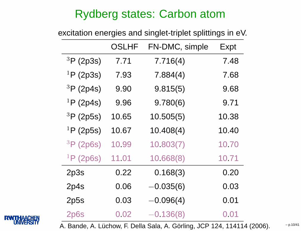
Rydberg states: Carbon atom

excitation energies and singlet-triplet splittings in eV.

OSLHF FN-DMC, simple Expt3P (2p3s) 7.71 7.716(4) 7.481P (2p3s) 7.93 7.884(4) 7.683P (2p4s) 9.90 9.815(5) 9.681P (2p4s) 9.96 9.780(6) 9.713P (2p5s) 10.65 10.505(5) 10.381P (2p5s) 10.67 10.408(4) 10.403P (2p6s) 10.99 10.803(7) 10.701P (2p6s) 11.01 10.668(8) 10.71

2p3s 0.22 0.168(3) 0.20

2p4s 0.06 −0.035(6) 0.03

2p5s 0.03 −0.096(4) 0.01

2p6s 0.02 −0.136(8) 0.01A. Bande, A. Lüchow, F. Della Sala, A. Görling, JCP 124, 114114 (2006). – p.10/41

nodal domains for C atom

analysis of nodal domains (not exhaustive) of C atom for current Slaterdeterminants from OSLHF/LYP orbitals

motivation: different domain energies? spurious nodes due toincomplete basis sets?

finding nodal domains:FN-DMC runs started with one walker only in arbitrary positions

importance of nodal domains:FN-DMC started with each walker of Ψ2

T VMC sample

averaging electron coordinates in each block

analysis for ground state and 1P (2p6s) state

– p.11/41


1P (2p6s) Rydberg state: domain energies and topologicalcharacterization

spin up spin down

EFN−DMC 〈r1〉〈r2〉〈r3〉〈r4〉〈r5〉〈r6〉Ω1 −37.4378(5) 1.5 1.5 1.5 1.1 1.1 1.1

Ω2 −37.4311(4) 43 1.5 0.3 1.1 1.1 1.1

Ω3 −37.4280(3) 20 1.5 0.3 1.1 1.1 1.1

Ω4 −37.4249(4) 10 1.5 0.3 1.1 1.1 1.1

Ω5 −36.563(1) 35 1.4 0.3 38 1.0 0.7

Ω6 −36.554(1) 46 1.4 0.3 30 1.4 0.3

energies in Eh and distances in bohr, individual standard deviations

excitation nodes: different domain energies

additionally spurious nodes: increase of FN-DMC excitation energy?

standard DMC calculation (random initial sample) ends in Ω1– p.12/41


if one electron is at large distance (“Rydberg electron”):

ΨN ≈ φnsΨN−1

excitation nodes as in atomic φns (hydrogen-like!)

Example 1P: φ6s radial distribution

3020100

0,03

0,02

0,01

0

-0,01r

-0,02

-0,03

5040

3020 50100

0,0025

r

0,0005

0,0015

40

0,001

0,002

0

– p.13/41

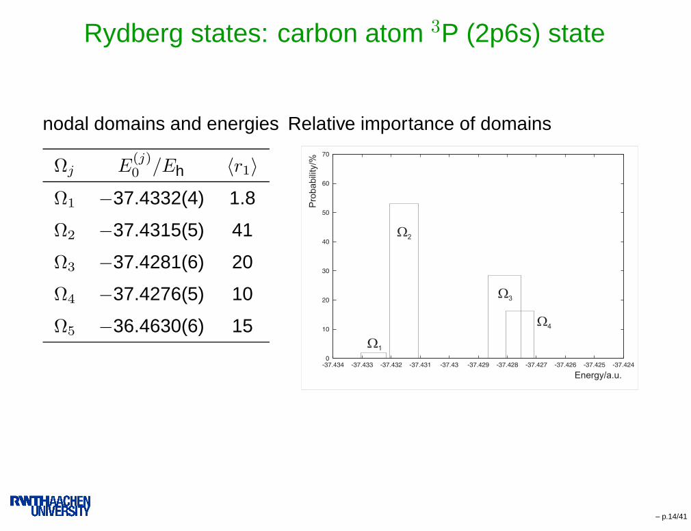
Rydberg states: carbon atom 3P (2p6s) state

nodal domains and energies

Ωj E(j)0 /Eh 〈r1〉

Ω1 −37.4332(4) 1.8

Ω2 −37.4315(5) 41

Ω3 −37.4281(6) 20

Ω4 −37.4276(5) 10

Ω5 −36.4630(6) 15

Relative importance of domains

– p.14/41

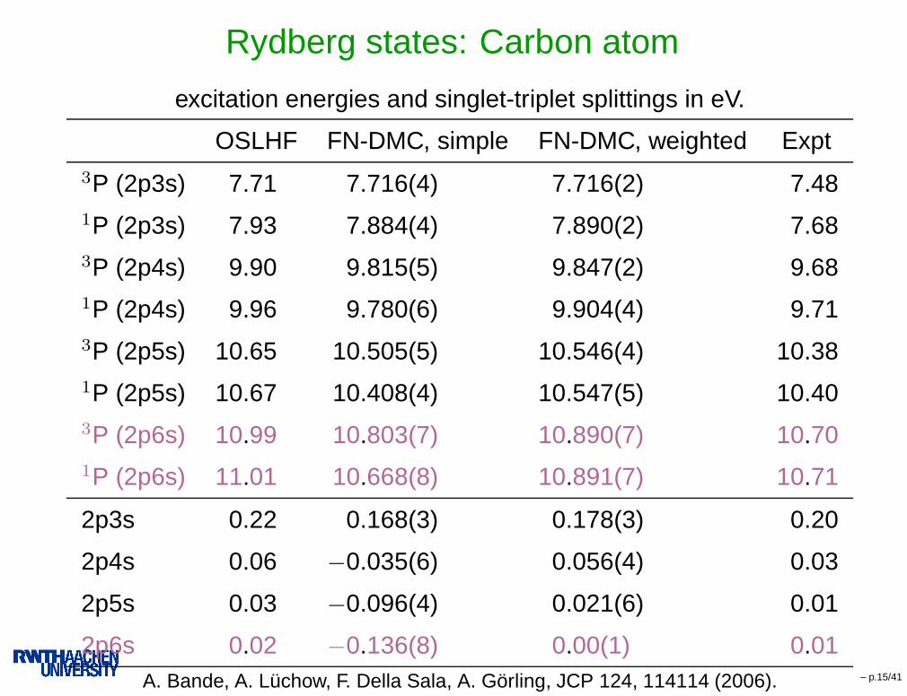
Rydberg states: Carbon atom

excitation energies and singlet-triplet splittings in eV.

OSLHF FN-DMC, simple FN-DMC, weighted Expt3P (2p3s) 7.71 7.716(4) 7.716(2) 7.481P (2p3s) 7.93 7.884(4) 7.890(2) 7.683P (2p4s) 9.90 9.815(5) 9.847(2) 9.681P (2p4s) 9.96 9.780(6) 9.904(4) 9.713P (2p5s) 10.65 10.505(5) 10.546(4) 10.381P (2p5s) 10.67 10.408(4) 10.547(5) 10.403P (2p6s) 10.99 10.803(7) 10.890(7) 10.701P (2p6s) 11.01 10.668(8) 10.891(7) 10.71

2p3s 0.22 0.168(3) 0.178(3) 0.20

2p4s 0.06 −0.035(6) 0.056(4) 0.03

2p5s 0.03 −0.096(4) 0.021(6) 0.01

2p6s 0.02 −0.136(8) 0.00(1) 0.01A. Bande, A. Lüchow, F. Della Sala, A. Görling, JCP 124, 114114 (2006). – p.15/41

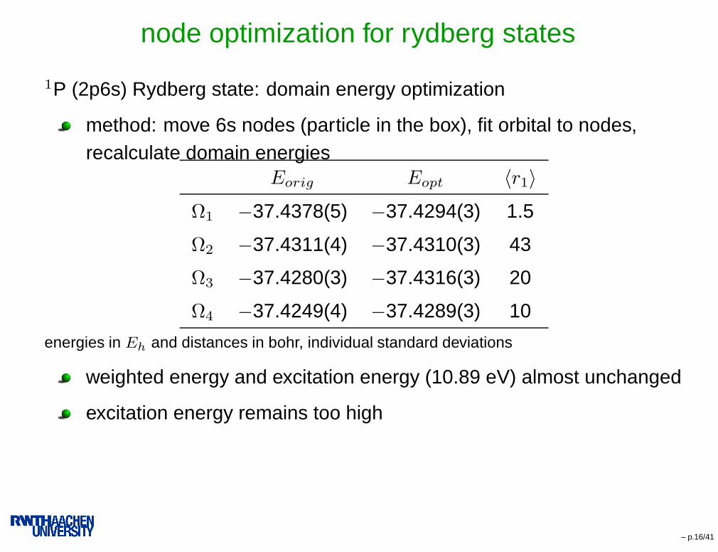
node optimization for rydberg states

1P (2p6s) Rydberg state: domain energy optimization

method: move 6s nodes (particle in the box), fit orbital to nodes,recalculate domain energies

Eorig Eopt 〈r1〉Ω1 −37.4378(5) −37.4294(3) 1.5

Ω2 −37.4311(4) −37.4310(3) 43

Ω3 −37.4280(3) −37.4316(3) 20

Ω4 −37.4249(4) −37.4289(3) 10


weighted energy and excitation energy (10.89 eV) almost unchanged

excitation energy remains too high

– p.16/41

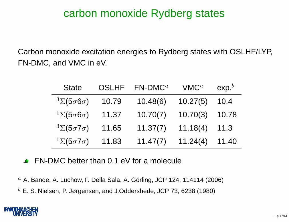
carbon monoxide Rydberg states

Carbon monoxide excitation energies to Rydberg states with OSLHF/LYP,FN-DMC, and VMC in eV.

State OSLHF FN-DMCa VMCa exp.b

3Σ(5σ6σ) 10.79 10.48(6) 10.27(5) 10.41Σ(5σ6σ) 11.37 10.70(7) 10.70(3) 10.783Σ(5σ7σ) 11.65 11.37(7) 11.18(4) 11.31Σ(5σ7σ) 11.83 11.47(7) 11.24(4) 11.40

FN-DMC better than 0.1 eV for a molecule

a A. Bande, A. Lüchow, F. Della Sala, A. Görling, JCP 124, 114114 (2006)b E. S. Nielsen, P. Jørgensen, and J.Oddershede, JCP 73, 6238 (1980)

– p.17/41

carbon monoxide Rydberg states

Carbon monoxide singlet-triplet splittings calculated with OSLHF/LYP,FN-DMC, and VMC in eV.

State OSLHF FN-DMC VMC exp.

(5σ6σ) 0.58 0.21(9) 0.43(6) 0.38

(5σ7σ) 0.18 0.10(9) 0.06(6) 0.10

– p.18/41

Fermion sign problem: direct improvement of nodes

current approach:

take nodal hypersurface from HF or KS Slater determinant (orMCSCF, CIS, PNOCI function) as fixed node

FN-DMC energy is determined by nodal hypersurface only (andvariational for the ground state)

BUT: nodal hypersurface obtained from energy minimization of

〈Ψ|H|Ψ〉 =∫

HΨ

ΨΨ2 dτ

⇒ good energies with inaccurate nodes possible

new idea: Direct optimization of the nodal hypersurface. But how?

local measure for the accuracy of the nodes

– p.19/41

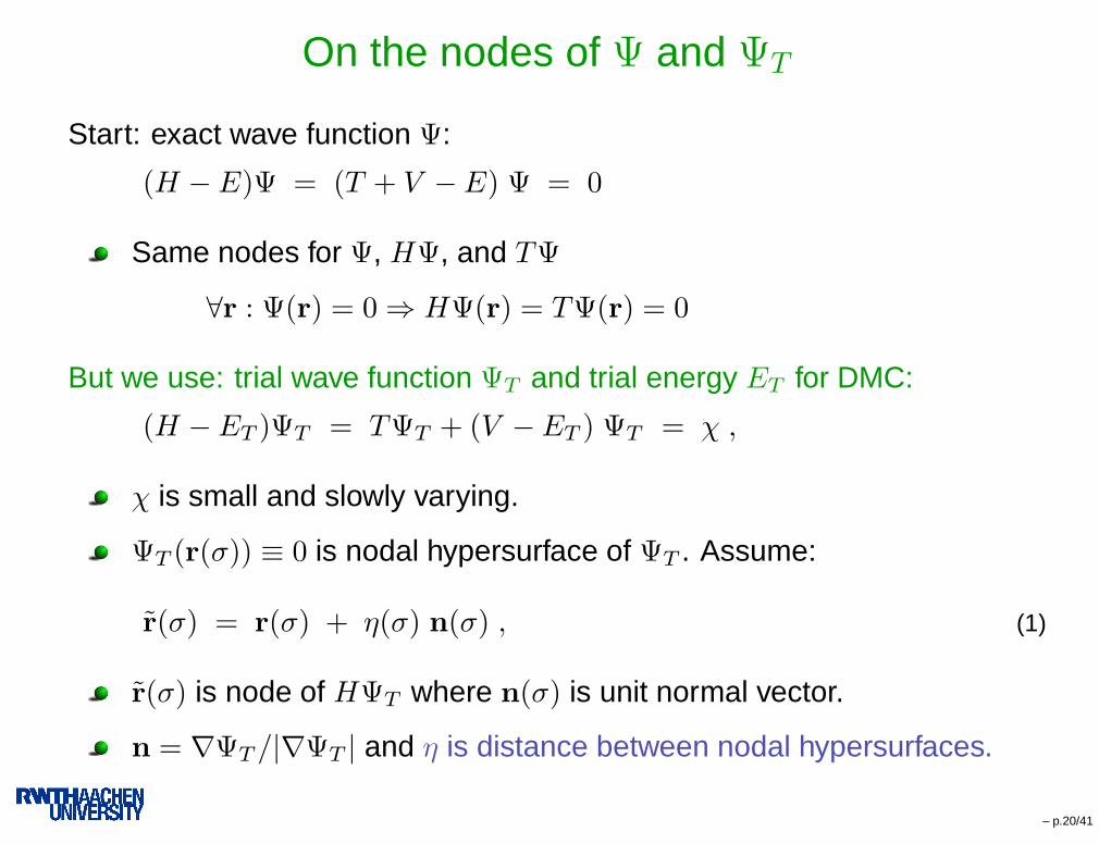
On the nodes of Ψ and ΨT

Start: exact wave function Ψ:

(H − E)Ψ = (T + V −E) Ψ = 0

Same nodes for Ψ, HΨ, and TΨ

∀r : Ψ(r) = 0⇒ HΨ(r) = TΨ(r) = 0

But we use: trial wave function ΨT and trial energy ET for DMC:

(H − ET )ΨT = TΨT + (V −ET ) ΨT = χ ,

χ is small and slowly varying.

ΨT (r(σ)) ≡ 0 is nodal hypersurface of ΨT . Assume:

r(σ) = r(σ) + η(σ) n(σ) , (1)

r(σ) is node of HΨT where n(σ) is unit normal vector.

n = ∇ΨT /|∇ΨT | and η is distance between nodal hypersurfaces.

– p.20/41

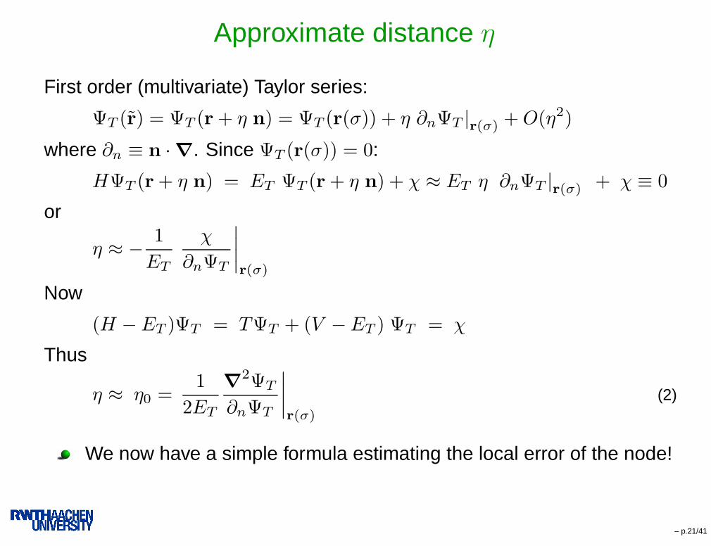
Approximate distance η

First order (multivariate) Taylor series:

ΨT (r) = ΨT (r + η n) = ΨT (r(σ)) + η ∂nΨT |r(σ) + O(η2)

where ∂n ≡ n ·∇. Since ΨT (r(σ)) = 0:

HΨT (r + η n) = ET ΨT (r + η n) + χ ≈ ET η ∂nΨT |r(σ) + χ ≡ 0

or

η ≈ − 1

ET

χ

∂nΨT

∣

∣

∣

∣

r(σ)

Now

(H − ET )ΨT = TΨT + (V −ET ) ΨT = χ

Thus

η ≈ η0 =1

2ET

∇2ΨT

∂nΨT

∣

∣

∣

∣

r(σ)

(2)

We now have a simple formula estimating the local error of the node!

– p.21/41

How accurate is distance approximation η0

plot of distance η (bisection) vs. approximation η0 for Be atom wavefunction (HF with Jastrow)

– p.22/41

Fermion sign problem: direct improvement of nodes

New approach:

determine quality of nodes locally (e.g. distance of nodes of Ψ = 0

and HΨ = 0, local variance)

improve nodes by parameter optimization for a sample of points atthe nodes (importance sampling)

most successful so far: estimate for the distance of nodal surface ofΨ = 0 and HΨ = 0:

η0 =1

2ET

∇2Ψ

∂nΨ

∣

∣

∣

∣

r(σ)

(3)

Minimization of sample mean: very inexpensive

η0 =

√

√

√

√

1

K

K∑

j=1

η0(rj)2 (4)

Levenberg-Marquardt-method applicable for many parameters

– p.23/41

direct improvement of nodes: first results

-0.4 -0.3 -0.2 -0.1 0.0 0.1c

-14.670

-14.665

-14.660

-14.655

-14.650

-14.645

-14.640

fixed

nod

e en

ergy

/ a.u

.

-0.4 -0.3 -0.2 -0.1 0.0 0.1c

0.003

0.004

0.005

mea

n di

stan

ces

η,η 0 /

bohr

-0.7 -0.6 -0.5 -0.4 -0.3 -0.2 -0.1 0 0.1c

0.00135

0.00140

0.00145

mea

n di

stan

ce η

0 / bo

hr

-0.7 -0.6 -0.5 -0.4 -0.3 -0.2 -0.1 0 0.1c

-75.900

-75.880

-75.860

fixed

nod

e en

ergy

/a.u

.

Successfully optimized a 2 CSF wave function for Be atom and C2

molecule

In the case of C2: better nodes than with MCSCF wave function

Allows finding “best” nodal hypersurface (lowest node location error)for a given wave function ansatz

a A. Lüchow, R. Petz, T.C. Scott, JCP 126, 144110 (2007) – p.24/41

Other Splittings and Bound

Similarly, get distance ξ between nodal hypersurfaces of ΨT and TΨT :

1

2

∇2ΨT

ξ∂nΨT

∣

∣

∣

∣

r(σ)

≈ ET −∂n(V ΨT )

∂nΨT

or ξ ≈ −TΨT

(ET − V )∂nΨT − (∂nV )ΨT

.

Establish Newton-Raphson (NR) scheme

ri+1 = ri + ei n,

where r0 = r(σ) and the error of ith iteration is:

ei(E, Ψ) =−TΨ(ri)

(E − V )∂nΨ(ri) − (∂nV )Ψ(ri)(5)

Self-Consistent NR scheme: ei(ET , ΨT ) where ΨT is updated withthe improved nodes at each iteration i.e. ΨT (r; ri+1)← ΨT (r; ri).

Iteration requires fitting of trial wave function to new nodes.

– p.25/41

Self-consistent Newton-Raphson scheme

Error |ei| of Self-Consistent Newton-Raphson scheme (SCNR) in bohr:

i Hydrogen 3s statea Hooke’s Atomb He 2 3S(1s2s)c

0 0.660851e-1 0.3192854 0.13614731 0.8242796e-2

5 0.161150e-2 0.3838903e-2 0.5172530e-3 0.5349413e-2

10 0.609075e-4 0.1431900e-3 0.2130606e-5 0.3480515e-2

15 0.228432e-5 0.5369231e-5 0.8778382e-8 0.2267004e-2

20 0.856610e-7 0.2013420e-6 0.3616815e-10 0.1477277e-2

aTrial nodes 1.93833 . . . , 6.63309 . . .→ True nodes 32 (3±

√3)

bTrial node at r12 = −2.2→ True node r12 = −2.cTrial node at s = 1.0, u = 0.5, t = −0.1→ True node t = 0.a T.C. Scott, A. Lüchow, J. Phys. B, 40, 851 (2007)

– p.26/41

Vanadium Oxides with Quantum Monte Carlo

transition metal compounds are often difficult for computational chemistry

strong non-dynamical correlation due to excitations within d shell

many electronic states close to ground state

strong dynamical correlation

relativistic contributions

standard ab initio techniques:

HF fails to describe non-dynamical correlation

MP2 often very inaccurate

Coupled cluster techniques often fairly accurate (but expensive)

DFT often surprisingly good

multireference method with dynamical correlation desired

MRCI, CASPT2

– p.27/41


why QMC?

dynamical correlation with Jastrow correlation factor

non-dynamical correlation with multi-determinant guide functions

but: large numbers of determinants expensive

relativistic effects with (localized) scalar relativistic pseudo potential

good scaling behaviour compared to coupled cluster or MRCImethods

– p.28/41


this investigation:

VO,VO2,VO3,VO4,V2O5 and its cations as examples

How accurate is QMC with single determinant?

Which orbitals are best for guide function?

Can KS orbitals catch non-dynamical correlation for DMC?

Stuttgart scalar relativistic PP for V

new Burkatzki/Dolg QMC-PP for O

– p.29/41


BP86/TZVP optimized geometries. Bond lengths are given in Å.

– p.30/41


Atomization energies in eV for VO and VO2:

VO VO2

Expt 6.51(20) 12.37

DMC/BP86 6.51(1) 11.83(2)

DMC/B3LYP 6.26(1) 11.58(2)

B3LYP 6.53 11.97

CCSD(T) 6.21 10.88

better accuracy with BP86 than B3LYP nodes

single reference DMC more accurate than CCSD(T)

– p.31/41


Oxygen abstraction energies in eV: VO(+)2 → V(+)O + O

VO2 VO+2

Expt 5.83(28) 3.60(36)

DMC/BP86 5.32(2) 3.90(1)

B3LYP 5.45 4.03

CCSD(T) 4.67 4.24

– p.32/41


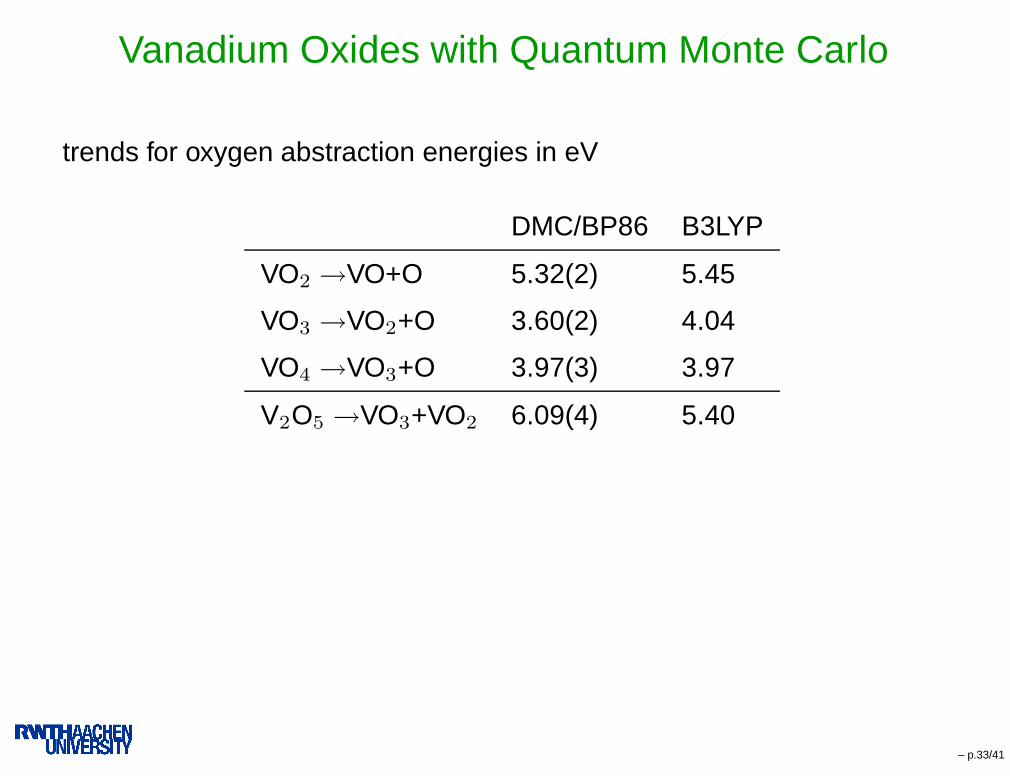
trends for oxygen abstraction energies in eV

DMC/BP86 B3LYP

VO2 →VO+O 5.32(2) 5.45

VO3 →VO2+O 3.60(2) 4.04

VO4 →VO3+O 3.97(3) 3.97

V2O5 →VO3+VO2 6.09(4) 5.40

– p.33/41


vertical and adiabatic ionization potential in eV

VO (v) VO (a)

Expt 7.31(1) 7.2386(4)

DMC/BP86 7.24(1) 7.17(1)

B3LYP 7.42 7.37

CCSD(T) 7.03 7.00

– p.34/41

Conclusions

conclusions:

FN-DMC for excited states possible. But: careful if domain energiesdiffer

solution: average over (many) DMC runs starting from individualwalkers of VMC sample

excitation energies with accuracy of 0.1 eV possible for Rydbergstates

direct optimization of nodes can be done by minimizing distance ofnodes of ΨT and HΨT for model problems.

direct node optimization successful for few atoms and molecules

good accuracy for vanadium oxides with only one determinantobtained: at least as good as CCSD(T)

higher accuracy of few systems would require multireference DMC– p.35/41

Acknowledgements

Annika Bande, RWTH Aachen university

Tony Scott, RWTH Aachen university

Christian Dietrich, Münster university

Collaborations:

Stefan Grimme, Münster

Andreas Görling, Erlangen

Fabio Della Sala, Lecce, Italy

Reinhold Fink, Würzburg

Financial support:

from Deutsche Forschungsgemeinschaft (DFG)

– p.36/41

DMC: Computational Details and Effort

Algorithm (part):

calculate AOs at current electron position(cubic splines, cusp correction)

calculate MOs from AOsor: direct 3d-interpolation for MOs

calculate Φdet(r) as (sum of) determinant(s)using LU decomposition

also: ∇Φdet(r),∇2Φdet(r)

updating algorithm

same for eU,∇e

U,∇2eU

calculate EL(r) = −∇2ΦG(r)

2ΦG(r)+ V(r)

– p.37/41

QMC: cusp correction for standard basis functions

GTOs have no cusp at nucleus→ fluctuating local energy nearnucleus

contracted GTO basis sets do not work for QMC(without pseudo potentials)→ use STO basis

standard contracted GTO basis sets can be used aftercusp correction:– exponential near nucleus, interpolating polynomial, rest unchanged– corrected basis function replaced by cubic splines

– p.38/41

QMC: cusp correction for standard basis functions

cusp correction for carbon 1s cc-pVTZ basis functionand its 2nd derivative:

using standard all-electron ab initio wavefunctions with QMC

or ECPs, but: only localized ECPs possible, localization Wloc =WΦG

ΦG

S. Manten and A. Lüchow, JCP 115, 5362 (2001)

– p.39/41

FN-DMC: carbon clusters

DMC/HF calculations for carbon clusters C20

ring bowl cage

S. Sokolova, A. Lüchow, J. B. Anderson, Chem. Phys. Lett. 323, 299 (2000) – p.40/41

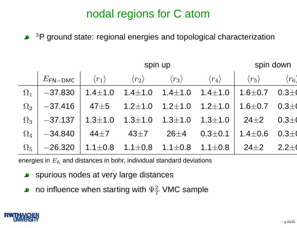
nodal regions for C atom

3P ground state: regional energies and topological characterization

spin up spin down

EFN−DMC 〈r1〉〈r2〉〈r3〉〈r4〉〈r5〉〈r6〉Ω1 −37.830 1.4±1.0 1.4±1.0 1.4±1.0 1.4±1.0 1.6±0.7 0.3±0.1

Ω2 −37.416 47±5 1.2±1.0 1.2±1.0 1.2±1.0 1.6±0.7 0.3±0.1

Ω3 −37.137 1.3±1.0 1.3±1.0 1.3±1.0 1.3±1.0 24±2 0.3±0.1

Ω4 −34.840 44±7 43±7 26±4 0.3±0.1 1.4±0.6 0.3±0.1

Ω5 −26.320 1.1±0.8 1.1±0.8 1.1±0.8 1.1±0.8 24±2 2.2±0.8


spurious nodes at very large distances

no influence when starting with Ψ2T VMC sample

– p.41/41

Documents

Quantum Monte Carlo calculations on Rydberg states … · QMC workshop, The Towler Institute, ... Importance sampled DMC algorithm: ... node optimization for rydberg states 1P