This content has been downloaded from IOPscience. Please scroll down to see the full text.

Download details:

IP Address: 193.205.206.85

This content was downloaded on 04/07/2016 at 21:20

Please note that terms and conditions apply.

Quantum interference in an asymmetric Mach-Zehnder interferometer

View the table of contents for this issue, or go to the journal homepage for more

2016 J. Opt. 18 085201

(http://iopscience.iop.org/2040-8986/18/8/085201)

Home Search Collections Journals About Contact us My IOPscience

Quantum interference in an asymmetricMach-Zehnder interferometer

A Trenti, M Borghi, M Mancinelli, H M Price, G Fontana and L Pavesi

Department of Physics, University of Trento, via Sommarive 14, Trento 38123, Italy

E-mail: alessandro.trenti@unitn.it

Received 24 March 2016, revised 17 May 2016Accepted for publication 31 May 2016Published 4 July 2016

AbstractA re-visitation of the well known free space Mach-Zehnder interferometer is reported here. Thecoexistence between one-photon and two-photons interference from collinear color entangledphoton pairs is investigated. Thisarises from an arbitrarily small unbalance in the armtransmittance. The tuning of such asymmetry is reflected in dramatic changes in the coincidencedetection, revealing beatings between one particle and two particle interference patterns. Inparticular, the role of the losses and of the intrinsic phase imperfectness of the lossy beamsplitterare explored in a single-port excited Mach-Zehnder interferometer. This configuration isespecially useful for quantum optics on a chip, where the guiding geometry forces photons totravel in the same spatial mode.

Keywords: quantum optics, quantum interferometry, color entangled photons, nonlinear optics

(Some figures may appear in colour only in the online journal)

1. Introduction

In recent years, advances in the generation of stable quantumstates of light by spontaneous parametric down conversion(SPDC) allowed to reinterpret several interferometricexperiments from a quantum optical point of view [1–4].Nonclassical interference has been observed in Michelson,Mach-Zehnder (MZ), Franson and Hong Ou Mandel (HOM)geometries [5–8]. Among these, the MZ structure receivedgrowing attentions due to its scalability in modern quantumoptical integrated circuits [9–11]. However, despite the sim-plicity of the device, not all the possibilities have beenexplored. In most of the cases, the symmetric configuration,where the MZ is excited at both ports of the input beamsplitter, has been considered [8, 12, 13]. In this case, thephoton pair is never split after the entrance beamsplitter dueto HOM effect [5], thus reducing the number of indis-tinguishable paths leading to a coincidence detection. Fur-thermore, it was assumed that the propagation characteristics(transmittance, losses, etc) of the two arms of the inter-ferometer were the same. On one hand, this simplificationoffers a more direct insight on the physics of the problem, butat the same time it hides the possibility to observe novelinteractions between single and two photon correlations.

In this work, we revisited the classical Mach-Zehnderinterferometer by assuming asymmetry and losses to enableall the different interference possibilities. In fact, we report onthe realization of an interference experiment in a Mach-Zehnder device where all the symmetries are removed. A pairof 1550 nm colour-entangled photons produced by type-0SPDC (i.e. both the down converted photons are co-polarizedand collinear with the pump ones) in a crystal of periodicallypoled lithium niobate (PPLN) enters in the same input port ofthe interferometer. Photon antibunching (split) and bunching(N00N) states, are created after the first beam splitter, and thestrength of their self and mutual interaction is changed bytuning the asymmetry of the transmittance between the twoarms. When bunching-bunching interactions are suppressed,the coincidence detection pattern, which is monitored as afunction of the time delay between the arms, shows only oneparticle interference fringes. On the contrary, the period of thelatter is doubled when antibunching-bunching interactionscancel, creating a two particle interference pattern. When allthe interactions act simultaneously, mixed patterns, showingat the same time beatings between single-photon, two-photonand Hong Ou Mandel interference, are observed. It is worthnoting that, while all these interference effects have beenpreviously reported [5, 8, 14], it has never addressed theimpact of the arm and of the beamsplitter losses on their

Journal of Optics

J. Opt. 18 (2016) 085201 (7pp) doi:10.1088/2040-8978/18/8/085201

2040-8978/16/085201+07$33.00 © 2016 IOP Publishing Ltd Printed in the UK1

interplay in the same coincidence pattern. The phase imper-fectness induced by the presence of the beamsplitter lossesplays a role in determining the outcome of our interferometricquantum optical experiment. The assumption of a lossy beamsplitter was essential to reproduce the experimental data withthe theoretical model. Our treatment is particularly relevantfor applications of quantum optic concepts in integrateddevices, since the waveguiding geometry itself forces the twophotons of the pair to travel in the same spatial direction, i.ethey are collinear at the input port of the MZ.

The paper is organized as follows: in section 2, thetheoretical model of the MZ is presented, and the probabilityof a coincidence photodetection is derived in terms of anunbalancing parameter. The experimental setup used tovalidate the model predictions will be outlined in section 3.The experimental results will be discussed in section 4.

2. Model

With reference to figure 1(a), the probability per unit time ofcoincidence detections at the output ports C and D of the MZat times t and t+t is given by [15]:

t t t= á + + ñ- - + +

P K E t E t E t E t 1D C C D( ) ˆ ( ) ˆ ( ) ˆ ( ) ˆ ( ) ( )

in which K is a constant which depends on the photodetectors,while

+ECˆ and

+EDˆ are respectively the positive frequency parts

of the electric field operator at the output ports C and D of theinterferometer. The expectation value of expression (1) iscalculated on state:

òyb

w w f w wñ = ñ + ñw wd d a a02

, 0 2s i s iin s i∣ ∣ ( ) ˆ ˆ ∣ ( )† †

which represents the two photon state produced by the SPDC.The process splits a pump photon at frequency w̃ into a signaland an idler photon at frequencies ws and wi respectively [5].

In equation (2), β is a constant which is proportional to theaverage number of pump photons in a second [16]. Thefunction f w w,s i( ) in equation (2) is the biphoton wavefunc-tion [16], which is normalized in such a way that

ò w w f w w =d d , 1s i s i2∣ ( )∣ . In what follows, we will consider

the pump field as monochromatic, since its coherence time isassumed to greatly exceeds the one of the down convertedphotons. As a consequence of this approximation, we can usethe energy conservation relation w w w= +s i˜ to express thefrequency of one photon of the pair as ω, and the frequency ofthe twin photon as w w-˜ . In this way, the biphotonwavefunction, which we assume to be Gaussian, can bewritten as:

f w w f wp s

= - w ws

-

e,1

3s i4

2 2

2 2( ) ( ) ( )( ˜ )

in which σ is the bandwidth of the generated photons. Thestate in equation (2) is sent to the input beamsplitter BS1,which, for simplicity, is described by the frequencyindependent amplitude reflectance and transmittance para-meters r1 and t1. The two arms of the MZ have differentpropagation losses gh and gr (defined as the ratio between theelectric field at the input ports of BS2 and the electric field atthe output ports of BS1), and a relative time delay tD . Thesubscript h comes from the fact that we will use an electronicheater to vary tD in the experiment described in section 4,while the subscript r indicates the reference arm. The outputbeamsplitter BS2 has amplitude reflectivity r2j and amplitudetransmittivity t2j, where =j C D, refer to the output ports ofBS2. This notation allows BS2 to be not symmetric withrespect to the input beams A and B, e.g. the reflectivity from Ato C (r2C) can be different with respect to the reflectivity fromB to D (r2D). We point out that, in our case, such asymmetryis not attributed to an intrinsic unbalance of the BS2transmittance/reflectance, but is induced by independentlytuning the position of the focusing lenses in front of thedetectors C and D. This is purposely done in order tointroduce a given asymmetry in the interferometer and,therefore, to allow studying its effect in the coincidence rates.For both BS1 and BS2, we will assume an equal phasedifference δ between the transmitted and reflected waves. Therange of variability of δ, as discussed in appendix B, isdetermined by the magnitude of losses [17]. In the mostfamiliar case of a lossless beamsplitter, d p= 2 [18].

The electric fields EC and ED can be written as:

g t gg g t

= - D += + - D

d

d d

- - - -

- - - - -

E t r r e E t t t E t

E t t r e E t r t e E t 4C h c

ir c

D r di

h di

1 22

in 1 2 in

1 2 in 1 2 in

( ) ( ) ( )( ) ( ) ( ) ( )

where -Ein is the negative frequency part of the input electricfield operator at BS1. By inserting a completeness relationbetween t+-E tC ( ) and t++E tD ( ) in equation (1), and byusing equation (4) we find:

t g g t tg g tg g t t tg g t t

= á + - D ñ

+ á + ñ

+ á - D + - D ñ

+ á - D + ñ

d

d

d

d

- - -

- - -

- - -

- - -

P K e E t E t

e E t E t

e E t E t

e E t E t 5

hc rdi

rd rci

hc hdi

hd rci

3in in

in in3

in in

in in2

( ) ∣ ( ) ( )( ) ( )

( ) ( )( ) ( ) ∣ ( )

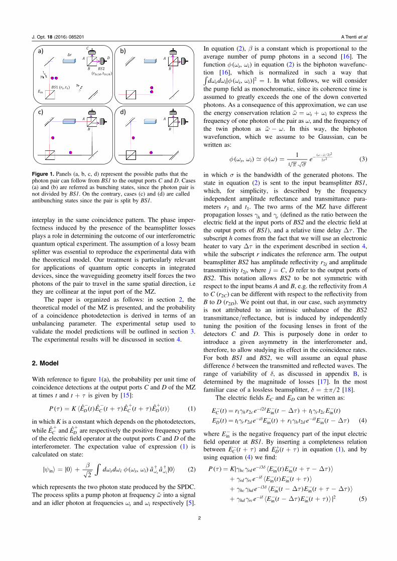
Figure 1. Panels (a, b, c, d) represent the possible paths that thephoton pair can follow from BS1 to the output ports C and D. Cases(a) and (b) are referred as bunching states, since the photon pair isnot divided by BS1. On the contrary, cases (c) and (d) are calledantibunching states since the pair is split by BS1.

2

J. Opt. 18 (2016) 085201 A Trenti et al

where the expectation values are now evaluated between theinitial state Y ñin∣ and the vacuum state ñ0∣ , i.eá ¢ ñ = áY ¢ ñ- - - -E t E t E t E t 0in in in in in( ) ( ) ∣ ( ) ( )∣ . In equation (5) wehave introduced the parameters:

g g g gg g g g

= == =

r r r tt t t r 6

hc h C hd h D

rc r C rd r D

1 2 1 2

1 2 1 2 ( )

where the subscript h r, refers to the path along the upper orlower arm of the interferometer respectively, while subscriptc d, denotes whether the photon arrives at detector C or D.The expectation values in equation (5) can be evaluated byusing the Fourier representation of the negative frequencypart of the input electric field:

ò w= ww-E t a e d 7i t

in( ) ( )†

and hence that:

fá ¢ ñ = - ¢ w- - ¢E t E t t t e2 8i tin in( ) ( ) ( ) ( )˜

where f t( ) is the Fourier transform of f w( ). Substitutingequation (8) into equation (5), we obtain that

t µ + + +P p p p ph h r r h rR

h rT

, , , ,2( ) ∣ ∣( ) ( ) , where:

g= w t d- D + -s tp r t r e e2 9h h D C h

i, 1

22 2

2 32 22 ( )( ˜ )

g= d- -s tp t t r e e2 10r r C D r

i, 1

22 2

2 2 22 ( )

g g= d- + -w t s t tD -Dp r t r r e e2 11h r

RC D h r

i, 1 1 2 2

32

2 2

2( ) ( )( ) ˜ ( )

g g= d- + -w t s t tD +Dp r t t t e e2 12h r

TC D h r

i, 1 1 2 2 2

2 2

2( ) ( )( ) ˜ ( )

The amplitude probabilities in equations (9)–(12) areassociated to well defined physical paths that the photon paircan follow from BS1 to ports C and D. These are sketched infigure 1. Consider for example the case in figure 1(a), whichis described by equation (9): both signal and idler are reflectedat BS1 and bunched into the upper arm of the MZ (r1

2), andexperience the same losses (gh

2). Then one photon is reflectedto port C while the other is transmitted to the port D at BS2(t rD C2 2 ). While travelling in the upper arm, they acquire an

overall phase factor w t- De i ˜ . The factor -s te

2 22 accounts for the

fact that the two photons are localized in time within theircoherence time t =

sc1 . Similar reasoning applies to the cases

when both photons are transmitted at BS1 (figure 1(b) andequation (10)) or when the pair is split (figures 1(c), (d) andequations (11)–(12)). The difference in the paths described byph r

R,

( ) and ph rT,

( ) comes from the fact that the pair reaches theoutput ports undergoing two reflections or two transmissionsat BS2 respectively. The factor two in all the amplitudeprobabilities takes into account the fact that the system issymmetric for the exchange of signal and idler photons. It isworth noting that the coincidence measurement correspondsto an integration with respect to τ over the coincidenceresolving time of a few nanoseconds of our detectors, whichis much longer than the photon correlation time. After per-forming the modulus square of the sum of the four transition

amplitudes in equations (9)–(12) and integrating, one findsthat the coincidence rate Nc is given by:

tD = ¢ + +N K C C C 13c 1 2 3( ) ( ) ( )

where ¢K is a constant and the three terms on the right handside are defined as follows:

g g g g d= + + ws t- DC A e2 cos 2 14hc rd hd rc1

2 2 2 2 2 2 ( ) ( )˜

g g g g w t d= + + D -wC A2 cos 2 15hc hd rc rd22 2 2 2 ( ˜ ) ( )˜

⎜ ⎟

⎜ ⎟

⎡⎣⎢

⎛⎝

⎞⎠

⎛⎝

⎞⎠

⎤⎦⎥

w t d

w t

=D +

+D

w

w

-s tDC e A

A

2 cos2

cos2

. 16

3 21

22

2 24

˜

˜ ( )

˜( )

˜( )

In equations (14)–(16) we have adopted the followingdefinitions:

g g g g=wA 17rc rd hc hd ( )˜

g g g g= +wA 18hc rc rd hd21 2 2( ) ( )˜

( )

g g g g= +wA . 19hd rd hc rc22 2 2( ) ( )˜

( )

It is also convenient to introduce the power amplitudecoefficient wA 2˜ associated to the frequency component at w

2

˜ :

d= + +w w w w wA A A A A2 cos 2 . 2022

21 2

22 2

21

22( ) ( ) ( ) ( )˜ ˜

( )˜( )

˜( )

˜( )

Equation (14) represents the antibunching-antibunchinginteraction between the paths (c) and (d) in figure 1, resultingin the well-known HOM dip at the optical contact of the MZ( tD = 0). Equation (15) describes the bunching-bunchinginteraction between the paths (a) and (b) in figure 1, which ismediated by the coupling strength wA ˜ . This term oscillates atfrequency w̃ which is two times the average single photonfrequency (w 2˜ ) and is responsible of two photon inter-ference. Finally equation (16) comes from the interferencebetween the bunching cases with the antibunching ones, andis mediated by the interaction parameter wA 2˜ . This inter-ference channel is missing in a balanced MZ or in a MZwhich is fed symmetrically at the two input ports due to acompletely destructive quantum interference [8, 12, 13]. Thisterm shows fringes at w 2˜ , creating a single photon inter-ference pattern. This comes from the fact that the phase dif-ference between the bunching and the antibunching cases isalways w tD2( ˜ ) . In fact, from the comparison of the paths(a-b) in figure 1 with the ones in figures 1(c)–(d), one cannotice that there is always one arm of the interferometerwhich carries one more photon with respect to the other. Thesame happens when a single photon enters at the input of BS1:it can take either the lower arm or the upper one, giving arelative phase of w tD2( ˜ ) between the two paths. In general,the coincidence pattern exhibits competing effects betweensingle and two particle interference, where their relative vis-ibility can be evaluated by the magnitude of an unbalancing

3

J. Opt. 18 (2016) 085201 A Trenti et al

parameter x = w wA A2˜ ˜ . Without losing any generality, wecan now restrict to the case of a lossless beamsplitter, inwhich d = p

2. In this case equation (20) simplifies

to g g g g g g g g= - -wA hc rd rc hd hc hd rc rd22 ( )( )˜ .In the limiting case where x ¥, the coincidence rate

shows no signs of two photon correlations. This can occur whenone of the four loss factor in equation (6) is equal to zero. If weconsider for example the case g = 0hc , then the photon whichfires the detector at port C is forced to come from the lower arm,providing a which-path information. The remaining uncertaintybetween the paths which the other photon of the pair may taketo fire the other detector, gives raise to pure single photoninterference. The lack of two photon correlations can be alsoexplained from the fact that when g = 0hc , the bunching path infigure 1(a) is suppressed, so bunching-bunching interactions(which are the source of two photon correlations) cancel. In theopposite case where x 0, antibunching-bunching interactionscancel out. This happens when some symmetries are imposedon the arm losses or on the beamsplitter coefficients. Thesimplest case is when both the beamsplitters are 50/50 devicesand the two arms have the same losses. We then haveg g g g= = =hc hd rc rd and consequently =wA 02˜ . Thus, onlyone frequency is observed when the device is ideal symmetric,which is consistent with what found in previous works [8, 12].There exist actually three other possible configurations forwhich antibunching-bunching interactions cancel:

i. Considering BS2 perfectly balanced, in this caseg g=hc hd and g g=rd rc.

ii. Imposing BS1 balanced and, at the same time, the armloss gr and gh to be equal, in this case g g=hc rcand g g=rd hd .

iii. Imposing that the transmittance from the input to port Cwhile travelling in the upper arm is equal to thetransmittance of its symmetric path (g g=rd hc) or vice-versa (g g=hd rc).

The presence of beamsplitter loss imped a completecancellation of the antibunching-bunching term. However, itis again the balanced configuration which minimizes thisinterference effect. Intermediate values of ξ can be realized bychanging the relative arm transmittance.

3. Experimental setup

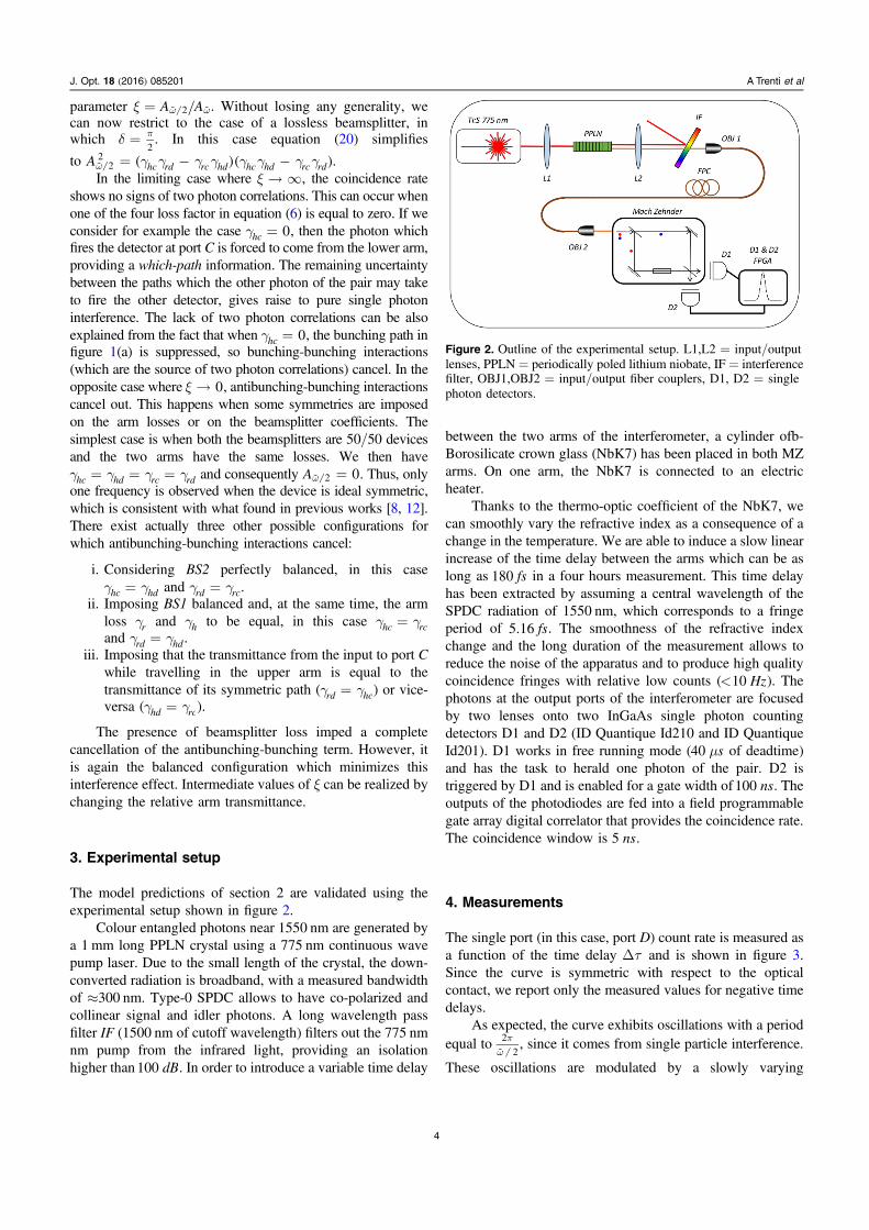
The model predictions of section 2 are validated using theexperimental setup shown in figure 2.

Colour entangled photons near 1550 nm are generated bya 1 mm long PPLN crystal using a 775 nm continuous wavepump laser. Due to the small length of the crystal, the down-converted radiation is broadband, with a measured bandwidthof ≈300 nm. Type-0 SPDC allows to have co-polarized andcollinear signal and idler photons. A long wavelength passfilter IF (1500 nm of cutoff wavelength) filters out the 775 nmnm pump from the infrared light, providing an isolationhigher than dB100 . In order to introduce a variable time delay

between the two arms of the interferometer, a cylinder ofb-Borosilicate crown glass (NbK7) has been placed in both MZarms. On one arm, the NbK7 is connected to an electricheater.

Thanks to the thermo-optic coefficient of the NbK7, wecan smoothly vary the refractive index as a consequence of achange in the temperature. We are able to induce a slow linearincrease of the time delay between the arms which can be aslong as fs180 in a four hours measurement. This time delayhas been extracted by assuming a central wavelength of theSPDC radiation of 1550 nm, which corresponds to a fringeperiod of fs5.16 . The smoothness of the refractive indexchange and the long duration of the measurement allows toreduce the noise of the apparatus and to produce high qualitycoincidence fringes with relative low counts (< Hz10 ). Thephotons at the output ports of the interferometer are focusedby two lenses onto two InGaAs single photon countingdetectors D1 and D2 (ID Quantique Id210 and ID QuantiqueId201). D1 works in free running mode ( ms40 of deadtime)and has the task to herald one photon of the pair. D2 istriggered by D1 and is enabled for a gate width of ns100 . Theoutputs of the photodiodes are fed into a field programmablegate array digital correlator that provides the coincidence rate.The coincidence window is ns5 .

4. Measurements

The single port (in this case, port D) count rate is measured asa function of the time delay tD and is shown in figure 3.Since the curve is symmetric with respect to the opticalcontact, we report only the measured values for negative timedelays.

As expected, the curve exhibits oscillations with a periodequal to p

w2

2˜, since it comes from single particle interference.

These oscillations are modulated by a slowly varying

Figure 2. Outline of the experimental setup. L1,L2 = input/outputlenses, PPLN = periodically poled lithium niobate, IF = interferencefilter, OBJ1,OBJ2 = input/output fiber couplers, D1, D2 = singlephoton detectors.

4

J. Opt. 18 (2016) 085201 A Trenti et al

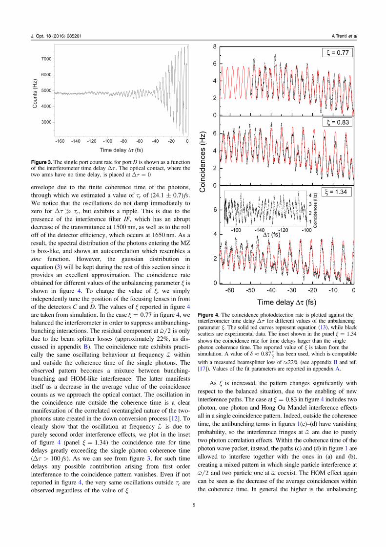
envelope due to the finite coherence time of the photons,through which we estimated a value of tc of fs24.1 0.7( ) .We notice that the oscillations do not damp immediately tozero for t tD c, but exhibits a ripple. This is due to thepresence of the interference filter IF, which has an abruptdecrease of the transmittance at 1500 nm, as well as to the rolloff of the detector efficiency, which occurs at 1650 nm. As aresult, the spectral distribution of the photons entering the MZis box-like, and shows an autocorrelation which resembles asinc function. However, the gaussian distribution inequation (3) will be kept during the rest of this section since itprovides an excellent approximation. The coincidence rateobtained for different values of the unbalancing parameter ξ isshown in figure 4. To change the value of ξ, we simplyindependently tune the position of the focusing lenses in frontof the detectors C and D. The values of ξ reported in figure 4are taken from simulation. In the case x = 0.77 in figure 4, webalanced the interferometer in order to suppress antibunching-bunching interactions. The residual component at w 2˜ is onlydue to the beam splitter losses (approximately 22%, as dis-cussed in appendix B). The coincidence rate exhibits practi-cally the same oscillating behaviour at frequency w̃ withinand outside the coherence time of the single photons. Theobserved pattern becomes a mixture between bunching-bunching and HOM-like interference. The latter manifestsitself as a decrease in the average value of the coincidencecounts as we approach the optical contact. The oscillation inthe coincidence rate outside the coherence time is a clearmanifestation of the correlated orentangled nature of the two-photons state created in the down conversion process [12]. Toclearly show that the oscillation at frequency w̃ is due topurely second order interference effects, we plot in the insetof figure 4 (panel x = 1.34) the coincidence rate for timedelays greatly exceeding the single photon coherence time( tD > fs100 ). As we can see from figure 3, for such timedelays any possible contribution arising from first orderinterference to the coincidence pattern vanishes. Even if notreported in figure 4, the very same oscillations outside tc areobserved regardless of the value of ξ.

As ξ is increased, the pattern changes significantly withrespect to the balanced situation, due to the enabling of newinterference paths. The case at x = 0.83 in figure 4 includes twophoton, one photon and Hong Ou Mandel interference effectsall in a single coincidence pattern. Indeed, outside the coherencetime, the antibunching terms in figures 1(c)–(d) have vanishingprobability, so the interference fringes at w̃ are due to purelytwo photon correlation effects. Within the coherence time of thephoton wave packet, instead, the paths (c) and (d) in figure 1 areallowed to interfere together with the ones in (a) and (b),creating a mixed pattern in which single particle interference atw 2˜ and two particle one at w̃ coexist. The HOM effect againcan be seen as the decrease of the average coincidences withinthe coherence time. In general the higher is the unbalancing

Figure 3. The single port count rate for port D is shown as a functionof the interferometer time delay tD . The optical contact, where thetwo arms have no time delay, is placed at tD = 0

Figure 4. The coincidence photodetection rate is plotted against theinterferometer time delay tD for different values of the unbalancingparameter ξ. The solid red curves represent equation (13), while blackscatters are experimental data. The inset shown in the panel x = 1.34shows the coincidence rate for time delays larger than the singlephoton coherence time. The reported value of ξ is taken from thesimulation. A value of d » p0.87

2has been used, which is compatible

with a measured beamsplitter loss of »22% (see appendix B and ref.[17]). Values of the fit parameters are reported in appendix A.

5

J. Opt. 18 (2016) 085201 A Trenti et al

between the arms, the higher is the suppression of the two-photon contribution at w̃ and, at the same time, the higher thevisibility of the single-photon component at w 2˜ . We see fromfigure 4 that it is sufficient to induce a value of x = 1.34 topractically cancel out the oscillation at w̃ within the coherencetime. In all the three cases shown in figure 4, simulations (solidred curves) well matches the experiment only if the phase δ

slightly deviates from p2

d = p0.872( ), i.e, if one assume that the

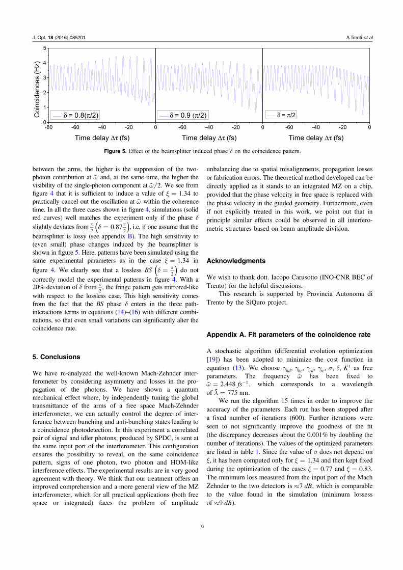
beamsplitter is lossy (see appendix B). The high sensitivity to(even small) phase changes induced by the beamsplitter isshown in figure 5. Here, patterns have been simulated using thesame experimental parameters as in the case x = 1.34 in

figure 4. We clearly see that a lossless BS d = p2( ) do not

correctly model the experimental patterns in figure 4. With a20% deviation of δ from p

2, the fringe pattern gets mirrored-like

with respect to the lossless case. This high sensitivity comesfrom the fact that the BS phase δ enters in the three path-interactions terms in equations (14)–(16) with different combi-nations, so that even small variations can significantly alter thecoincidence rate.

5. Conclusions

We have re-analyzed the well-known Mach-Zehnder inter-ferometer by considering asymmetry and losses in the pro-pagation of the photons. We have shown a quantummechanical effect where, by independently tuning the globaltransmittance of the arms of a free space Mach-Zehnderinterferometer, we can actually control the degree of inter-ference between bunching and anti-bunching states leading toa coincidence photodetection. In this experiment a correlatedpair of signal and idler photons, produced by SPDC, is sent atthe same input port of the interferometer. This configurationensures the possibility to reveal, on the same coincidencepattern, signs of one photon, two photon and HOM-likeinterference effects. The experimental results are in very goodagreement with theory. We think that our treatment offers animproved comprehension and a more general view of the MZinterferometer, which for all practical applications (both freespace or integrated) faces the problem of amplitude

unbalancing due to spatial misalignments, propagation lossesor fabrication errors. The theoretical method developed can bedirectly applied as it stands to an integrated MZ on a chip,provided that the phase velocity in free space is replaced withthe phase velocity in the guided geometry. Furthermore, evenif not explicitly treated in this work, we point out that inprinciple similar effects could be observed in all interfero-metric structures based on beam amplitude division.

Acknowledgments

We wish to thank dott. Iacopo Carusotto (INO-CNR BEC ofTrento) for the helpful discussions.

This research is supported by Provincia Autonoma diTrento by the SiQuro project.

Appendix A. Fit parameters of the coincidence rate

A stochastic algorithm (differential evolution optimization[19]) has been adopted to minimize the cost function inequation (13). We choose g g g g s d ¢K, , , , , ,hd hc rd rc as freeparameters. The frequency w̃ has been fixed tow = -fs2.448 ,1˜ which corresponds to a wavelengthof l = 775 nm˜ .

We run the algorithm 15 times in order to improve theaccuracy of the parameters. Each run has been stopped aftera fixed number of iterations (600). Further iterations wereseen to not significantly improve the goodness of the fit(the discrepancy decreases about the 0.001% by doubling thenumber of iterations). The values of the optimized parametersare listed in table 1. Since the value of σ does not depend onξ, it has been computed only for x = 1.34 and then kept fixedduring the optimization of the cases x = 0.77 and x = 0.83.The minimum loss measured from the input port of the MachZehnder to the two detectors is » dB7 , which is comparableto the value found in the simulation (minimum lossessof » dB9 ).

Figure 5. Effect of the beamsplitter induced phase δ on the coincidence pattern.

6

J. Opt. 18 (2016) 085201 A Trenti et al

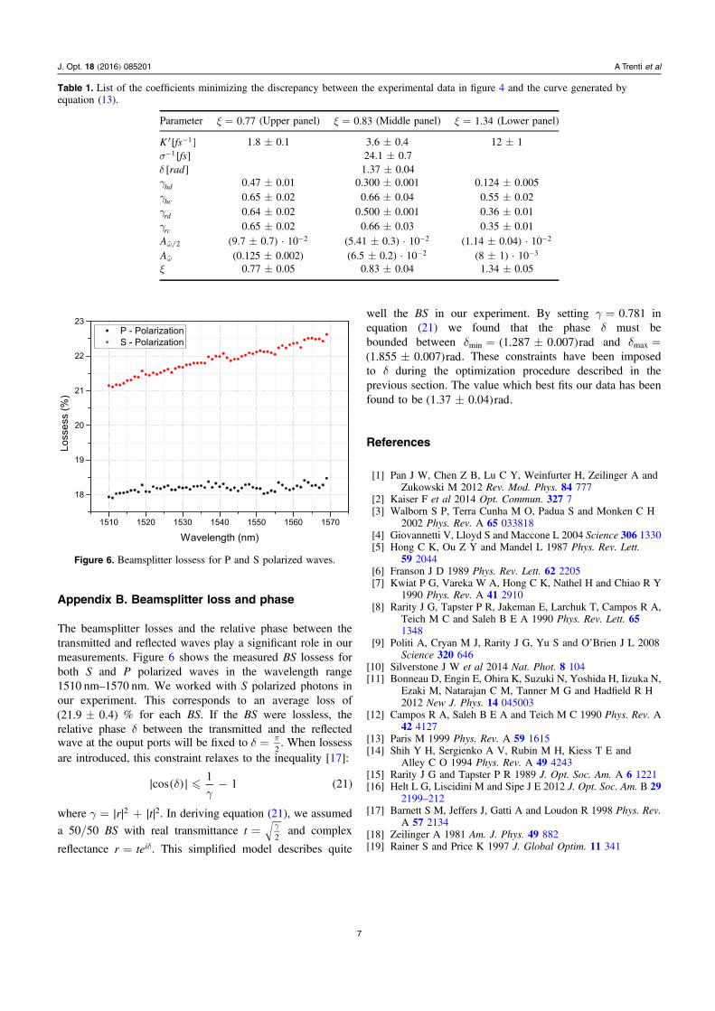
Appendix B. Beamsplitter loss and phase

The beamsplitter losses and the relative phase between thetransmitted and reflected waves play a significant role in ourmeasurements. Figure 6 shows the measured BS lossess forboth S and P polarized waves in the wavelength range1510 nm–1570 nm. We worked with S polarized photons inour experiment. This corresponds to an average loss of

21.9 0.4( ) % for each BS. If the BS were lossless, therelative phase δ between the transmitted and the reflectedwave at the ouput ports will be fixed to d = p

2. When lossess

are introduced, this constraint relaxes to the inequality [17]:

dg

-cos1

1 21∣ ( )∣ ( )

where g = +r t2 2∣ ∣ ∣ ∣ . In deriving equation (21), we assumed

a 50/50 BS with real transmittance = gt2

and complex

reflectance = dr tei . This simplified model describes quite

well the BS in our experiment. By setting g = 0.781 inequation (21) we found that the phase δ must bebounded between d = 1.287 0.007 radmin ( ) and d =max

1.855 0.007 rad( ) . These constraints have been imposedto δ during the optimization procedure described in theprevious section. The value which best fits our data has beenfound to be 1.37 0.04 rad( ) .

References

[1] Pan J W, Chen Z B, Lu C Y, Weinfurter H, Zeilinger A andZukowski M 2012 Rev. Mod. Phys. 84 777

[2] Kaiser F et al 2014 Opt. Commun. 327 7[3] Walborn S P, Terra Cunha M O, Padua S and Monken C H

2002 Phys. Rev. A 65 033818[4] Giovannetti V, Lloyd S and Maccone L 2004 Science 306 1330[5] Hong C K, Ou Z Y and Mandel L 1987 Phys. Rev. Lett.

59 2044[6] Franson J D 1989 Phys. Rev. Lett. 62 2205[7] Kwiat P G, Vareka W A, Hong C K, Nathel H and Chiao R Y

1990 Phys. Rev. A 41 2910[8] Rarity J G, Tapster P R, Jakeman E, Larchuk T, Campos R A,

Teich M C and Saleh B E A 1990 Phys. Rev. Lett. 651348

[9] Politi A, Cryan M J, Rarity J G, Yu S and O’Brien J L 2008Science 320 646

[10] Silverstone J W et al 2014 Nat. Phot. 8 104[11] Bonneau D, Engin E, Ohira K, Suzuki N, Yoshida H, Iizuka N,

Ezaki M, Natarajan C M, Tanner M G and Hadfield R H2012 New J. Phys. 14 045003

[12] Campos R A, Saleh B E A and Teich M C 1990 Phys. Rev. A42 4127

[13] Paris M 1999 Phys. Rev. A 59 1615[14] Shih Y H, Sergienko A V, Rubin M H, Kiess T E and

Alley C O 1994 Phys. Rev. A 49 4243[15] Rarity J G and Tapster P R 1989 J. Opt. Soc. Am. A 6 1221[16] Helt L G, Liscidini M and Sipe J E 2012 J. Opt. Soc. Am. B 29

2199–212[17] Barnett S M, Jeffers J, Gatti A and Loudon R 1998 Phys. Rev.

A 57 2134[18] Zeilinger A 1981 Am. J. Phys. 49 882[19] Rainer S and Price K 1997 J. Global Optim. 11 341

Table 1. List of the coefficients minimizing the discrepancy between the experimental data in figure 4 and the curve generated byequation (13).

Parameter x = 0.77 (Upper panel) x = 0.83 (Middle panel) x = 1.34 (Lower panel)

¢ -K fs 1[ ] 1.8 ± 0.1 3.6 ± 0.4 12 ± 1s- fs1[ ] 24.1 ± 0.7d rad[ ] 1.37 ± 0.04ghd 0.47 ± 0.01 0.300 ± 0.001 0.124 ± 0.005ghc 0.65 ± 0.02 0.66 ± 0.04 0.55 ± 0.02grd 0.64 ± 0.02 0.500 ± 0.001 0.36 ± 0.01grc 0.65 ± 0.02 0.66 ± 0.03 0.35 ± 0.01

wA 2˜ -9.7 0.7 10 2( ) · -5.41 0.3 10 2( ) · -1.14 0.04 10 2( ) ·wA ˜ 0.125 0.002( ) -6.5 0.2 10 2( ) · -8 1 10 3( ) ·

ξ 0.77 ± 0.05 0.83 ± 0.04 1.34 ± 0.05

Figure 6. Beamsplitter lossess for P and S polarized waves.

7

J. Opt. 18 (2016) 085201 A Trenti et al