Embed Size (px)
Citation preview

Quantum Information Science and QuantumMetrology: Novel Systems and Applications
The Harvard community has made thisarticle openly available. Please share howthis access benefits you. Your story matters
Citation Kómár, Péter. 2016. Quantum Information Science and QuantumMetrology: Novel Systems and Applications. Doctoral dissertation,Harvard University, Graduate School of Arts & Sciences.
Citable link http://nrs.harvard.edu/urn-3:HUL.InstRepos:26718726
Terms of Use This article was downloaded from Harvard University’s DASHrepository, and is made available under the terms and conditionsapplicable to Other Posted Material, as set forth at http://nrs.harvard.edu/urn-3:HUL.InstRepos:dash.current.terms-of-use#LAA
Quantum Information Science and QuantumMetrology: Novel Systems and Applications
A dissertation presented
by
Peter Komar
to
The Department of Physics
in partial fulfillment of the requirements
for the degree of
Doctor of Philosophy
in the subject of
Physics
Harvard University
Cambridge, Massachusetts
December 2015

c©2015 - Peter Komar
All rights reserved.
Thesis advisor Author
Mikhail D. Lukin Peter Komar
Quantum Information Science and Quantum Metrology:
Novel Systems and Applications
Abstract
The current frontier of our understanding of the physical universe is dominated
by quantum phenomena. Uncovering the prospects and limitations of acquiring and
processing information using quantum effects is an outstanding challenge in physical
science. This thesis presents an analysis of several new model systems and applications
for quantum information processing and metrology.
First, we analyze quantum optomechanical systems exhibiting quantum phenom-
ena in both optical and mechanical degrees of freedom. We investigate the strength of
non-classical correlations in a model system of two optical and one mechanical mode.
We propose and analyze experimental protocols that exploit these correlations for
quantum computation.
We then turn our attention to atom-cavity systems involving strong coupling of
atoms with optical photons, and investigate the possibility of using them to store
information robustly and as relay nodes. We present a scheme for a robust two-qubit
quantum gate with inherent error-detection capabilities. We consider several remote
entanglement protocols employing this robust gate, and we use these systems to study
the performance of the gate in practical applications.
iii
Abstract
Finally, we present a new protocol for running multiple, remote atomic clocks in
quantum unison. We show that by creating a cascade of independent Greenberger-
Horne-Zeilinger states distributed across the network, the scheme asymptotically
reaches the Heisenberg limit, the fundamental limit of measurement accuracy. We
propose an experimental realization of such a network consisting of neutral atom
clocks, and analyze the practical performance of such a system.
iv
Contents
Title Page . . . . . . . . . . . . . . . . . . . . . . . . . . . . . . . . . . . . iAbstract . . . . . . . . . . . . . . . . . . . . . . . . . . . . . . . . . . . . . iiiTable of Contents . . . . . . . . . . . . . . . . . . . . . . . . . . . . . . . . vList of Figures . . . . . . . . . . . . . . . . . . . . . . . . . . . . . . . . . . xiList of Tables . . . . . . . . . . . . . . . . . . . . . . . . . . . . . . . . . . xiiiCitations to Previously Published Work . . . . . . . . . . . . . . . . . . . xivAcknowledgments . . . . . . . . . . . . . . . . . . . . . . . . . . . . . . . . xvDedication . . . . . . . . . . . . . . . . . . . . . . . . . . . . . . . . . . . . xvii
1 Introduction and Motivation 11.1 Overview and Structure . . . . . . . . . . . . . . . . . . . . . . . . . 11.2 Optomechanical Systems . . . . . . . . . . . . . . . . . . . . . . . . . 31.3 Atom-Cavity Systems . . . . . . . . . . . . . . . . . . . . . . . . . . . 41.4 Quantum Repeaters . . . . . . . . . . . . . . . . . . . . . . . . . . . . 51.5 Atomic Clocks and Quantum Metrology . . . . . . . . . . . . . . . . 61.6 Rydberg Blockade . . . . . . . . . . . . . . . . . . . . . . . . . . . . . 9
2 Single-photon nonlinearities in two-mode optomechanics 112.1 Introduction . . . . . . . . . . . . . . . . . . . . . . . . . . . . . . . . 112.2 Multimode optomechanics . . . . . . . . . . . . . . . . . . . . . . . . 142.3 Equal-time correlations . . . . . . . . . . . . . . . . . . . . . . . . . . 17
2.3.1 Average transmission and reflection . . . . . . . . . . . . . . . 172.3.2 Intensity correlations . . . . . . . . . . . . . . . . . . . . . . . 202.3.3 Absence of two-photon resonance at ∆ = 0 . . . . . . . . . . . 232.3.4 Finite temperature . . . . . . . . . . . . . . . . . . . . . . . . 25
2.4 Delayed coincidence and single phonon states . . . . . . . . . . . . . 302.4.1 Driven mode . . . . . . . . . . . . . . . . . . . . . . . . . . . 312.4.2 Heralded single phonon states . . . . . . . . . . . . . . . . . . 34
2.5 Reaching strong coupling . . . . . . . . . . . . . . . . . . . . . . . . . 372.6 Conclusions . . . . . . . . . . . . . . . . . . . . . . . . . . . . . . . . 38
v
Contents
3 Optomechanical quantum information processing 403.1 Introduction . . . . . . . . . . . . . . . . . . . . . . . . . . . . . . . . 403.2 Model . . . . . . . . . . . . . . . . . . . . . . . . . . . . . . . . . . . 423.3 Resonant strong-coupling optomechanics . . . . . . . . . . . . . . . . 433.4 An OM single-photon source . . . . . . . . . . . . . . . . . . . . . . . 463.5 Single-phonon single-photon transistor . . . . . . . . . . . . . . . . . 473.6 Phonon-phonon interactions . . . . . . . . . . . . . . . . . . . . . . . 493.7 Conclusions . . . . . . . . . . . . . . . . . . . . . . . . . . . . . . . . 51
4 Heralded Quantum Gates with Integrated Error Detection 524.1 Introduction . . . . . . . . . . . . . . . . . . . . . . . . . . . . . . . . 524.2 Heralding gate . . . . . . . . . . . . . . . . . . . . . . . . . . . . . . . 544.3 Performance . . . . . . . . . . . . . . . . . . . . . . . . . . . . . . . . 56
4.3.1 Model . . . . . . . . . . . . . . . . . . . . . . . . . . . . . . . 564.3.2 Effective Hamiltonian . . . . . . . . . . . . . . . . . . . . . . . 574.3.3 Success probability . . . . . . . . . . . . . . . . . . . . . . . . 584.3.4 Gate time . . . . . . . . . . . . . . . . . . . . . . . . . . . . . 59
4.4 Additional errors . . . . . . . . . . . . . . . . . . . . . . . . . . . . . 604.5 Possible implementation . . . . . . . . . . . . . . . . . . . . . . . . . 624.6 Application . . . . . . . . . . . . . . . . . . . . . . . . . . . . . . . . 634.7 Conclusion . . . . . . . . . . . . . . . . . . . . . . . . . . . . . . . . . 64
5 Remote entanglement distribution using individual atoms in cavities 655.1 Introduction . . . . . . . . . . . . . . . . . . . . . . . . . . . . . . . . 655.2 High-fidelity quantum repeater . . . . . . . . . . . . . . . . . . . . . 68
5.2.1 Secret key rate . . . . . . . . . . . . . . . . . . . . . . . . . . 745.2.2 Repeater architecture . . . . . . . . . . . . . . . . . . . . . . . 76
5.3 Other cavity based repeaters . . . . . . . . . . . . . . . . . . . . . . . 785.3.1 Single-photon entanglement creation . . . . . . . . . . . . . . 785.3.2 Initial purification . . . . . . . . . . . . . . . . . . . . . . . . . 805.3.3 CNOT gates . . . . . . . . . . . . . . . . . . . . . . . . . . . . 82
5.4 Numerical optimization . . . . . . . . . . . . . . . . . . . . . . . . . . 845.5 Conclusion . . . . . . . . . . . . . . . . . . . . . . . . . . . . . . . . . 94
6 Heisenberg-Limited Atom Clocks Based on Entangled Qubits 976.1 Introduction . . . . . . . . . . . . . . . . . . . . . . . . . . . . . . . . 976.2 Feedback loop . . . . . . . . . . . . . . . . . . . . . . . . . . . . . . . 1036.3 Spectroscopic noises . . . . . . . . . . . . . . . . . . . . . . . . . . . 104
6.3.1 Phase estimation with multiple GHZ groups . . . . . . . . . . 1056.3.2 Optimization . . . . . . . . . . . . . . . . . . . . . . . . . . . 106
6.4 Comparison with other schemes . . . . . . . . . . . . . . . . . . . . . 107
vi
Contents
7 A quantum network of clocks 1117.1 Introduction . . . . . . . . . . . . . . . . . . . . . . . . . . . . . . . . 1117.2 The concept of quantum clock network . . . . . . . . . . . . . . . . . 1137.3 Preparation of network-wide entangled states . . . . . . . . . . . . . . 1167.4 Interrogation . . . . . . . . . . . . . . . . . . . . . . . . . . . . . . . 1187.5 Feedback . . . . . . . . . . . . . . . . . . . . . . . . . . . . . . . . . . 1207.6 Stability analysis . . . . . . . . . . . . . . . . . . . . . . . . . . . . . 1217.7 Security . . . . . . . . . . . . . . . . . . . . . . . . . . . . . . . . . . 1257.8 Outlook . . . . . . . . . . . . . . . . . . . . . . . . . . . . . . . . . . 126
8 Quantum network of neutral atom clocks 1308.1 Introduction . . . . . . . . . . . . . . . . . . . . . . . . . . . . . . . . 1308.2 Description of the protocol . . . . . . . . . . . . . . . . . . . . . . . . 132
8.2.1 Collective excitations . . . . . . . . . . . . . . . . . . . . . . . 1338.2.2 Non-local connection . . . . . . . . . . . . . . . . . . . . . . . 1338.2.3 Local connection . . . . . . . . . . . . . . . . . . . . . . . . . 1358.2.4 Local GHZ growing . . . . . . . . . . . . . . . . . . . . . . . . 136
8.3 Implementation . . . . . . . . . . . . . . . . . . . . . . . . . . . . . . 1388.4 Clock network optimization . . . . . . . . . . . . . . . . . . . . . . . 1408.5 Conclusion . . . . . . . . . . . . . . . . . . . . . . . . . . . . . . . . . 143
A Appendices for Chapter 2 144A.1 Derivation of reflected mode operator . . . . . . . . . . . . . . . . . . 144A.2 Analytic model . . . . . . . . . . . . . . . . . . . . . . . . . . . . . . 145
B Appendices for Chapter 3 148B.1 Phonon nonlinearities . . . . . . . . . . . . . . . . . . . . . . . . . . . 148
B.1.1 Model . . . . . . . . . . . . . . . . . . . . . . . . . . . . . . . 148B.1.2 Displaced frame . . . . . . . . . . . . . . . . . . . . . . . . . . 149B.1.3 Hybridized modes . . . . . . . . . . . . . . . . . . . . . . . . . 150B.1.4 Adiabatic elimination of the cavity mode . . . . . . . . . . . . 152B.1.5 Simple perturbation theory . . . . . . . . . . . . . . . . . . . 153B.1.6 Corrections . . . . . . . . . . . . . . . . . . . . . . . . . . . . 154B.1.7 Numerical simulation . . . . . . . . . . . . . . . . . . . . . . . 155
B.2 Phonon-phonon interactions . . . . . . . . . . . . . . . . . . . . . . . 157
C Appendices for Chapter 4 160C.1 Perturbation theory . . . . . . . . . . . . . . . . . . . . . . . . . . . . 160
C.1.1 Success probability and fidelity . . . . . . . . . . . . . . . . . 165C.1.2 N -qubit Toffoli gate . . . . . . . . . . . . . . . . . . . . . . . 165C.1.3 CZ-gate . . . . . . . . . . . . . . . . . . . . . . . . . . . . . . 167C.1.4 Two-photon driving . . . . . . . . . . . . . . . . . . . . . . . . 169
vii
Contents
C.2 Gate time . . . . . . . . . . . . . . . . . . . . . . . . . . . . . . . . . 172C.3 Numerical simulation . . . . . . . . . . . . . . . . . . . . . . . . . . . 174C.4 Additional errors . . . . . . . . . . . . . . . . . . . . . . . . . . . . . 177
D Appendices for Chapter 5 181D.1 Error analysis of the single-photon scheme . . . . . . . . . . . . . . . 181D.2 Error analysis of the two-photon scheme . . . . . . . . . . . . . . . . 183D.3 Deterministic CNOT gate . . . . . . . . . . . . . . . . . . . . . . . . 184D.4 Rate analysis . . . . . . . . . . . . . . . . . . . . . . . . . . . . . . . 186
D.4.1 Deterministic gates . . . . . . . . . . . . . . . . . . . . . . . . 189D.4.2 Probabilistic gates . . . . . . . . . . . . . . . . . . . . . . . . 192
E Appendices for Chapter 6 196E.1 Figure of merit: Allan-variance . . . . . . . . . . . . . . . . . . . . . 196E.2 Single-step Uncorrelated ensemble . . . . . . . . . . . . . . . . . . . . 198
E.2.1 Sub-ensembles and projection noise . . . . . . . . . . . . . . . 198E.2.2 Effects of laser fluctuations: Phase slip errors . . . . . . . . . 199E.2.3 Optimal Ramsey time . . . . . . . . . . . . . . . . . . . . . . 200
E.3 Cascaded interrogation using GHZ states . . . . . . . . . . . . . . . . 202E.3.1 Parity measurement . . . . . . . . . . . . . . . . . . . . . . . 203E.3.2 Failure of the maximally entangled GHZ . . . . . . . . . . . . 204E.3.3 Cascaded GHZ scheme . . . . . . . . . . . . . . . . . . . . . . 205E.3.4 Rounding errors: finding the optimal n0 . . . . . . . . . . . . 207E.3.5 Phase slip errors: limitations to the Ramsey time T from laser
noise . . . . . . . . . . . . . . . . . . . . . . . . . . . . . . . . 210E.3.6 Extending the Ramsey time beyond the laser noise limit . . . 211E.3.7 Individual qubit noise and final result . . . . . . . . . . . . . . 214
E.4 Analytic solution of xn = A exp[−1/x] . . . . . . . . . . . . . . . . . 215E.5 Upper bound on the tail of the distribution of the estimated phase . . 217
E.5.1 Upper bound on the tail of the binomial distribution . . . . . 218E.5.2 Upper bound on the distribution of the estimated phase . . . 219
E.6 Threshold fidelity . . . . . . . . . . . . . . . . . . . . . . . . . . . . . 221
F Appendices for Chapter 7 223F.1 GHZ cascade in a network of K clocks . . . . . . . . . . . . . . . . . 223
F.1.1 Parity measurement . . . . . . . . . . . . . . . . . . . . . . . 224F.1.2 Cascaded GHZ scheme . . . . . . . . . . . . . . . . . . . . . . 225F.1.3 Rounding errors . . . . . . . . . . . . . . . . . . . . . . . . . . 228F.1.4 Phase slip errors . . . . . . . . . . . . . . . . . . . . . . . . . 230F.1.5 Pre-narrowing the linewidth . . . . . . . . . . . . . . . . . . . 233F.1.6 Individual qubit dephasing noise . . . . . . . . . . . . . . . . . 234
F.2 Security countermeasures . . . . . . . . . . . . . . . . . . . . . . . . . 235
viii
Contents
F.2.1 Sabotage . . . . . . . . . . . . . . . . . . . . . . . . . . . . . . 235F.2.2 Eavesdropping . . . . . . . . . . . . . . . . . . . . . . . . . . . 236F.2.3 Rotating center role . . . . . . . . . . . . . . . . . . . . . . . . 237
F.3 Network operation . . . . . . . . . . . . . . . . . . . . . . . . . . . . 237F.3.1 Different degree of feedback . . . . . . . . . . . . . . . . . . . 237F.3.2 Timing . . . . . . . . . . . . . . . . . . . . . . . . . . . . . . . 238F.3.3 Dick effect . . . . . . . . . . . . . . . . . . . . . . . . . . . . . 239F.3.4 More general architectures . . . . . . . . . . . . . . . . . . . . 239F.3.5 Accuracy . . . . . . . . . . . . . . . . . . . . . . . . . . . . . 241F.3.6 Efficient use of qubits . . . . . . . . . . . . . . . . . . . . . . . 242F.3.7 Required EPR generation rate . . . . . . . . . . . . . . . . . . 242F.3.8 Threshold fidelity . . . . . . . . . . . . . . . . . . . . . . . . . 243
G Appendices for Chapter 8 245G.1 Overview of optimization . . . . . . . . . . . . . . . . . . . . . . . . . 245G.2 Local entangling errors . . . . . . . . . . . . . . . . . . . . . . . . . . 246
G.2.1 Imperfect blockade . . . . . . . . . . . . . . . . . . . . . . . . 246G.2.2 Decaying Rydberg states . . . . . . . . . . . . . . . . . . . . . 249G.2.3 Rydberg interaction induced broadening . . . . . . . . . . . . 249
G.3 Non-local entangling errors . . . . . . . . . . . . . . . . . . . . . . . . 253G.3.1 Imperfect blockade . . . . . . . . . . . . . . . . . . . . . . . . 253G.3.2 Rydberg state decay . . . . . . . . . . . . . . . . . . . . . . . 254G.3.3 Photon propagation and detection errors . . . . . . . . . . . . 254G.3.4 Memory loss . . . . . . . . . . . . . . . . . . . . . . . . . . . . 255G.3.5 Imperfect branching ratios . . . . . . . . . . . . . . . . . . . . 255
G.4 Implementation with Yb . . . . . . . . . . . . . . . . . . . . . . . . . 256G.4.1 Rydberg lifetimes . . . . . . . . . . . . . . . . . . . . . . . . . 256G.4.2 Self-blockade, ∆11 . . . . . . . . . . . . . . . . . . . . . . . . . 257G.4.3 Cross-blockade, ∆12 . . . . . . . . . . . . . . . . . . . . . . . . 257G.4.4 Decay rates of lower levels . . . . . . . . . . . . . . . . . . . . 258G.4.5 Photon channels . . . . . . . . . . . . . . . . . . . . . . . . . 258
G.5 Optimization . . . . . . . . . . . . . . . . . . . . . . . . . . . . . . . 258G.5.1 Optimal parameters . . . . . . . . . . . . . . . . . . . . . . . 259G.5.2 Comparison of error sources . . . . . . . . . . . . . . . . . . . 260
G.6 Clock precision . . . . . . . . . . . . . . . . . . . . . . . . . . . . . . 263G.6.1 Imperfect initialization . . . . . . . . . . . . . . . . . . . . . . 263G.6.2 Measurement . . . . . . . . . . . . . . . . . . . . . . . . . . . 264G.6.3 Fisher information . . . . . . . . . . . . . . . . . . . . . . . . 265G.6.4 Cramer-Rao bound . . . . . . . . . . . . . . . . . . . . . . . . 266G.6.5 Allan-deviation . . . . . . . . . . . . . . . . . . . . . . . . . . 267G.6.6 Comparison to non-entangled interrogation . . . . . . . . . . . 268G.6.7 Optimal clock network size . . . . . . . . . . . . . . . . . . . . 268
ix
Contents
G.7 Multiple local ensembles . . . . . . . . . . . . . . . . . . . . . . . . . 270G.8 Calculating Var(φj,k) . . . . . . . . . . . . . . . . . . . . . . . . . . . 272
G.8.1 Calculating 〈φj,k〉 . . . . . . . . . . . . . . . . . . . . . . . . . 272G.8.2 Calculating
⟨φ2j,k
⟩. . . . . . . . . . . . . . . . . . . . . . . . . 274
G.8.3 Result for Var(φj,k) . . . . . . . . . . . . . . . . . . . . . . . . 275G.9 Calculating Var(ψj) . . . . . . . . . . . . . . . . . . . . . . . . . . . . 275
G.9.1 Calculating 〈ψj〉 . . . . . . . . . . . . . . . . . . . . . . . . . . 275G.9.2 Calculating
⟨ψ2j
⟩. . . . . . . . . . . . . . . . . . . . . . . . . 276
G.9.3 Result for Var(ψj) . . . . . . . . . . . . . . . . . . . . . . . . 277G.10 Calculating Var(∆j) . . . . . . . . . . . . . . . . . . . . . . . . . . . 277
G.10.1 Calculating 〈∆j〉 . . . . . . . . . . . . . . . . . . . . . . . . . 278G.10.2 Calculating
⟨∆2j
⟩. . . . . . . . . . . . . . . . . . . . . . . . . 279
G.10.3 Result for Var(∆j) . . . . . . . . . . . . . . . . . . . . . . . . 280
Bibliography 281
x

List of Figures
2.1 Two-mode optomechanical system . . . . . . . . . . . . . . . . . . . . 142.2 Lower level diagram of 2+1 optomechanical system . . . . . . . . . . 162.3 Photon statistics in anti-symmetric mode, a . . . . . . . . . . . . . . 182.4 Photon statistics in symmetric mode, s . . . . . . . . . . . . . . . . . 192.5 Photon statistics in reflected mode, R . . . . . . . . . . . . . . . . . . 192.6 Illustration of dominant processes . . . . . . . . . . . . . . . . . . . . 222.7 Aggregate photon statistics . . . . . . . . . . . . . . . . . . . . . . . 252.8 Temperature dependence of the relevant levels . . . . . . . . . . . . . 262.9 Effect of non-zero temperature on photon statistics of mode a . . . . 262.10 Effect of non-zero temperature on photon statistics of mode s . . . . 272.11 Autocorrelation of mode a . . . . . . . . . . . . . . . . . . . . . . . . 332.12 Autocorrelation of mode s . . . . . . . . . . . . . . . . . . . . . . . . 352.13 Diagram of the metastable subspace . . . . . . . . . . . . . . . . . . . 36
3.1 Model of two resonators . . . . . . . . . . . . . . . . . . . . . . . . . 423.2 Behavior of the coupled system . . . . . . . . . . . . . . . . . . . . . 443.3 A single-phonon single-photon transistor . . . . . . . . . . . . . . . . 473.4 Controlled phase gate . . . . . . . . . . . . . . . . . . . . . . . . . . . 49
4.1 Level structures of qubit and control atoms . . . . . . . . . . . . . . . 564.2 Success probability . . . . . . . . . . . . . . . . . . . . . . . . . . . . 604.3 Level structure of auxiliary atom . . . . . . . . . . . . . . . . . . . . 61
5.1 The general architecture of a quantum repeater . . . . . . . . . . . . 695.2 Entanglement generation . . . . . . . . . . . . . . . . . . . . . . . . . 705.3 Schematics of the heralded CZ gate . . . . . . . . . . . . . . . . . . . 725.4 Secret key fraction . . . . . . . . . . . . . . . . . . . . . . . . . . . . 755.5 Number of swap levels . . . . . . . . . . . . . . . . . . . . . . . . . . 775.6 Purification . . . . . . . . . . . . . . . . . . . . . . . . . . . . . . . . 815.7 CNOT gate structure . . . . . . . . . . . . . . . . . . . . . . . . . . . 825.8 CNOT gates comparison . . . . . . . . . . . . . . . . . . . . . . . . . 86
xi
List of Figures
5.9 Example of repeater architecture . . . . . . . . . . . . . . . . . . . . 875.10 Optimal secret key rate I . . . . . . . . . . . . . . . . . . . . . . . . . 895.11 Optimal secret key rate II . . . . . . . . . . . . . . . . . . . . . . . . 90
6.1 GHZ cascade . . . . . . . . . . . . . . . . . . . . . . . . . . . . . . . 1016.2 Comparison of clock protocols . . . . . . . . . . . . . . . . . . . . . . 108
7.1 The concept of world-wide quantum clock network . . . . . . . . . . . 1157.2 Entangled state preparation between distant nodes . . . . . . . . . . 1177.3 Performance of different operation schemes . . . . . . . . . . . . . . . 1227.4 Schematics of security countermeasures . . . . . . . . . . . . . . . . . 127
8.1 Steps to generate of pairwise entanglement . . . . . . . . . . . . . . . 1348.2 Connecting links into non-local GHZ state . . . . . . . . . . . . . . . 1368.3 Local GHZ creation . . . . . . . . . . . . . . . . . . . . . . . . . . . . 1378.4 Implementation with Yb levels . . . . . . . . . . . . . . . . . . . . . . 139
B.1 Comparison of effective and exact description . . . . . . . . . . . . . 156
C.1 Level structure of qubit an auxiliary atoms . . . . . . . . . . . . . . . 162C.2 Error and success probability vs cooperativity . . . . . . . . . . . . . 168C.3 Level structure of auxiliary atom . . . . . . . . . . . . . . . . . . . . 169C.4 Gate time and success probability vs driving strength . . . . . . . . . 176C.5 Conditional fidelity . . . . . . . . . . . . . . . . . . . . . . . . . . . . 177C.6 Gate time and success probability vs detuning . . . . . . . . . . . . . 178
F.1 GHZ cascade protocol for K clocks . . . . . . . . . . . . . . . . . . . 226
G.1 Coupling through doubly excited states . . . . . . . . . . . . . . . . . 251G.2 Optimal parameter values . . . . . . . . . . . . . . . . . . . . . . . . 260G.3 Minimal error per atom . . . . . . . . . . . . . . . . . . . . . . . . . . 263G.4 Average Fisher information . . . . . . . . . . . . . . . . . . . . . . . 266G.5 Optimal network size . . . . . . . . . . . . . . . . . . . . . . . . . . . 269G.6 Maximal gain over classical schemes . . . . . . . . . . . . . . . . . . . 270G.7 Arc length in a circular cloud . . . . . . . . . . . . . . . . . . . . . . 273
xii
List of Tables
5.1 Characteristics of the three gates . . . . . . . . . . . . . . . . . . . . 845.2 Parameters in the numerical optimization . . . . . . . . . . . . . . . . 85
8.1 Error budget . . . . . . . . . . . . . . . . . . . . . . . . . . . . . . . 141
C.1 Comparison of CZ and Toffoli gates . . . . . . . . . . . . . . . . . . . 161C.2 Perturbation validity criteria . . . . . . . . . . . . . . . . . . . . . . . 173
G.1 Error budget of 2D setup . . . . . . . . . . . . . . . . . . . . . . . . . 261G.2 Error budget of 3D setup . . . . . . . . . . . . . . . . . . . . . . . . . 262
xiii
Citations to Previously Published Work
Most of the chapters of this thesis have appeared in print elsewhere. By chapternumber, they are:
• Chapter 2: “Single-photon nonlinearities in two-mode optomechanics,” P. Komar,S. D. Bennett, K. Stannigel, S. J. M. Habraken, P. Rabl, P. Zoller, and M. D.Lukin, Phys. Rev. A 87, 013839 (2013).
• Chapter 3: “Optomechanical Quantum Information Processing with Photonsand Phonons,” K. Stannigel, P. Komar, S. J. M. Habraken, S. D. Bennett, M.D. Lukin, P. Zoller, and P. Rabl, Phys. Rev. Lett. 109, 013603 (2012).
• Chapter 4: “Heralded Quantum Gates with Integrated Error Detection in Op-tical Cavities,” J. Borregaard, P. Komar, E. M. Kessler, A. S. Sørensen, and M.D. Lukin, Phys. Rev. Lett. 114, 110502 (2015).
• Chapter 5: “Long-distance entanglement distribution using individual atoms inoptical cavities,” J. Borregaard, P. Komar, E. M. Kessler, A. S. Sørensen, andM. D. Lukin, Phys. Rev. A 92, 012307 (2015).
• Chapter 6: “Heisenberg-Limited Atom Clocks Based on Entangled Qubits,” E.M. Kessler, P. Komar, M. Bishof, L. Jiang, A. S. Sørensen, J. Ye, and M. D.Lukin, Phys. Rev. Lett. 112, 190403 (2014).
• Chapter 7: “A quantum network of clocks,” P. Komar, E. M. Kessler, M. Bishof,L. Jiang, A. S. Sørensen, J. Ye, and M. D. Lukin, Nature Physics 10, 582587(2014).
• Chapter 8: “Quantum network of neutral atom clocks,” P. Komar, T. Topcu, E.M. Kessler, A. Derevianko, V. Vuletic, J. Ye, and M. D. Lukin, in preparation.
xiv
Acknowledgments
First of all, I would like to thank my research advisor, Prof. Mikhail Lukin, for his
scientific insights and ideas, and especially for his attention and patience in guiding
my work and education.
I would like to thank other members of my thesis committee, Prof. John Doyle
and Prof. Subir Sachdev, with whom I was fortunate to work as a teaching fellow.
Their knowledge and thoroughness inspired both my teaching and research.
I am grateful to Prof. Andrei Derevianko at University of Nevada, Prof. Liang
Jiang at Yale, Prof. Pierre Meystre at University of Arizona, Prof. Peter Rabl in
Vienna, Till Rosenband at Harvard, Prof. Anders Sørensen in Copenhagen, Prof.
Vladan Vuletic at MIT, Prof. Jun Ye at JILA, and Prof. Peter Zoller in Innsbruck
for the enlightening discussions and their invaluable contributions to my research in
the past five years.
I would like to thank all colleagues with whom I worked namely, Michael Bishof,
Soonwon Choi, Manuel Endres, Ruffin Evans, Michael Goldman, Michael Gullans,
Steven Habraken, Marton Kanasz-Nagy, Shimon Kolkowitz, Ronen Kroeze, Peter
Maurer, Travis Nicholson, Janos Perczel, Thibault Peyronel, Arthur Safira, Alp
Sipahigil, Kai Stannigel, Alex Sushkov, Jeff Thompson, Turker Topcu, Dominik
Wild, Norman Yao, Leo Zhou. I am especially grateful to Steven Bennett, Johannes
Borregaard, and Eric Kessler; besides many years of fruitful collaboration, they helped
me as mentors and friends.
I would also like to thank David Morin, Jacob Barandes, Nick Schade and people
from the Bok Center, John Girash, Colleen Noonan, and Matthew Sussman, for their
efforts in guiding me to become a better teacher.
xv

Acknowledgments
I am thankful for my friends in Cambridge and Boston: Travis and John Woolcott,
who gave me tremendous help during my first year, and continued to keep an eye on
me; Bence Beky and Margit Szabari for teaching me the tricks and traditions of living
in the US; and Kartiek Agarwal, Debanjan Chowdhury and Ilya Feige for our endless
discussions about life.
The Physics Department staff has been an invaluable resource. I would like to
thank Monika Bankowski, Jennifer Bastin, Lisa Cacciabaudo, Karl Coleman, Carol
Davis, Sheila Ferguson, Joan Hamilton, Dayle Maynard, Clare Ploucha, Janet Ragusa
and Sarah Roberts, for helping me at countless occasions.
I am grateful to the Harvard International Office, and especially to Darryl Zeigler,
for facilitating my stay at Harvard.
I am thankful to the Office of Career Services, and especially Laura Stark and
Heather Law, for helping me transition to the next stage of my career.
Finally, I would like to thank my family, Erzsebet and Antal Komar, Anna Komar
and Szilvia Kiriakov, for their immense support and understanding towards my edu-
cation and work. I cannot thank you enough. This thesis is dedicated to you.
xvi
Dedicated to my parents Erzsebet and Antal,
my sister Anna,
and my fiancee Szilvia.
xvii
Chapter 1
Introduction and Motivation
1.1 Overview and Structure
The field of quantum science aims to answer conceptual and practical questions
about the fundamental behavior, controllability and applicability of systems governed
by quantum physics. Such systems arise whenever a few degrees of freedom of a
physical system become isolated from their environment.
Realizing and maintaining the required isolation is a formidable task. The inter-
action within the isolated components needs to be much stronger than the collective
coupling to modes of the environment. Once achieved, the system starts to explore
an expanded set of states: Its dynamics are not constrained to a countable number of
pointer (or “classical”) states anymore, originally selected by the environment, rather
it moves around smoothly in the entire Hilbert space, with its motion governed by
a Hamilton operator. Internal components of such a system are said to be “strongly
coupled”, and their dynamics to be “coherent”.
1
Chapter 1: Introduction and Motivation
The variety of (“quantum”) states in the Hilbert space gives rise to counter-
intuitive phenomena such as superposition, tunneling and entanglement. Besides
being academically exciting, these phenomena hold the promise that future devices
and protocols relying on them will perform better than any conceivable scheme based
solely on classical dynamics.
The discovery of efficient quantum algorithms for problems that are conjectured
to not be efficiently computable fueled the field of Quantum Computing. In Chapters
2 and 3, we analyze the capabilities of nano-scale optomechanical systems to perform
coherent logical operations, the elemental steps of quantum computation.
Protocols that rely on entanglement to distribute secret keys between distant
parties are the main focus of Quantum Communication. Their security is based
on fundamental physical limitations, rather than practical limitations arising from
computational complexity. In Chapters 4 and 5, we describe how a system consisting
of a few atoms isolated in an optical cavity can be used to realize a quantum gate with
integrated error detection, and we analyze its usefulness in a quantum communication
setup.
The idea of preparing a detector in a quantum superposition in order to focus its
sensitivity to the quantity of interest is the central topic of Quantum Metrology. In
Chapters 6, 7 and 8, we present a protocol for operating a network of atomic clocks,
which combines local and remote entanglement to surpass the accuracy of classical
protocols and asymptotically reach the fundamental quantum limit of precision, the
Heisenberg limit.
2
Chapter 1: Introduction and Motivation
1.2 Optomechanical Systems
The current fabrication technology allows the creation of integrated devices with
nanometer-scale features such as waveguides [148], photonic band-gap materials [88],
non-linear inductive elements [139], antenna arrays [241], optical cavities [165], and
mechanical resonators of various shapes and sizes [10].
Coupling components with different physical properties can give rise to devices
which incorporate the best characteristics of each component. Optical components
are fast (∼ 100 − 1000 THz) and fairly isolated, but making them strongly interact
with each other is challenging [45]. Mechanical components, on the other hand, are
much slower (∼ 0.01 − 10 GHz), but are usually much more sensitive to changes in
their surroundings [10]. One successful application is using mechanical elements as
transducers between two optical degrees of freedom for efficient filtering and frequency
conversion [79], while driven by classical light.
The interaction between a light field and a mechanical surface originates mainly
from the light-pressure displacing the mechanics. This gives rise to a non-linear
parametric coupling between light intensity and mechanical motion [150]. In Chapter
2, we analyze a quantum model of two optical cavities and a mechanical oscillator
interacting through this coupling. We find that if the system is driven by a weak
laser pulse (accurately described by a Poisson-process of photon arrivals), the output
light exhibits super- and sub-Poissonian characteristics. We find that if the system
is properly tuned, and is sufficiently cooled down, then it can be used for coherent
quantum operations. If the energy difference between the two optical modes is bridged
by the mechanical mode, then we can use the photons leaving the output port with
3
Chapter 1: Introduction and Motivation
the lower frequency to herald the creation of a single mechanical excitation.
Using oscillators as quantum registers in a future quantum computer requires them
to be anharmonic [138]. This is because consecutive levels of an anharmonic oscillator
are separated by unequal frequency intervals, which makes it possible to address
transitions independently. The inherent non-linearity of the optomechanical coupling
holds the promise of rendering the coupled oscillator system sufficiently anharmonic
for computational tasks. In Chapter 3, we propose a quantum logic architecture
based on coupled optomechanical components. We find that, under sufficiently strong
cooling, the system exhibits non-classical behavior and is able to store information
and perform logic gates on the qubits.
1.3 Atom-Cavity Systems
Coupling individual atoms to optical cavities is one of the most effective ways to
realize a well-controllable and manifestly quantum system [137, 231]. The first model,
named after E. Jaynes and F. Cummings [111, 204], describes the coherent dynamics
of a single transition between two levels of an atom and a single, confined optical
mode. This model is exactly solvable and serves as a great source of intuition.
As the physical size of an optical cavity is decreased, the zero-point electric field
corresponding to the ground state of its modes increases. As a result, individual
atoms placed inside such a cavity, coupled through their electric dipole moment,
start to interact strongly with the optical modes. Once this interaction becomes
much stronger than the coupling of the atoms to the radiation environment outside
of the cavity, the system becomes strongly coupled, and their states hybridize. From
4
Chapter 1: Introduction and Motivation
a spectroscopic point of view, this results in a resolvable splitting of the optical
resonances.
Optical cavities built on photonic crystal waveguides [220] have high zero-point
electric fields, and produce couplings to atoms larger than their spontaneous emission
rate. Their observed lifetime is then considerably decreased [81]; an effect called
Purcell-enhancement. Once such strong interaction is demonstrated, the prospect
of using these systems for coherent quantum logic operations becomes realistic. In
Chapter 4, we consider a model of three atoms placed inside and coupled by a single
optical cavity. We show that with tailored driving pulses and a proper choice of atomic
levels this system can perform a controlled-NOT operation on two of the atoms and
can be made tolerant to the dominating error, caused by the loss of a photon, by
post-selecting on the state of the third atom.
1.4 Quantum Repeaters
Creating quantum entanglement between systems separated by large distances is
the most important prerequisite of quantum communication protocols. Experimen-
tal realizations rely on exchanging weak light pulses via carefully monitored optical
fibers [167]. The reliability of direct transmission of photon pulses is limited by the
fiber attenuation length, the maximum of which (∼ 20 km) is achieved at telecom
wavelength (∼ 1.5µm).
Classical communication solves the attenuation problem by incorporating fiber
segments which amplify the signal. Conceptually, this classical amplification relies on
detecting some of the signal photons and emitting more in synchrony. Unfortunately,
5
Chapter 1: Introduction and Motivation
such a process fails for quantum channels using single-photon pulses, because the
detection event can measure the photon only once, therefore it necessarily discards
essential information about its quantum state.
Overcoming the attenuation problem in quantum channels requires using more
resources. The scheme of quantum repeaters consists of repeater stations placed be-
tween the sender and the receiver [17, 18, 70]. These stations, instead of relaying the
information forward, create pairwise entanglement with their neighbors using direct
photon transmission via fibers, which are much shorter than the total length. Once
all entangled pairs are heralded, each station performs a local quantum logic oper-
ation between the two pairs that they have access to. This is called entanglement
connection, resulting in entanglement between the two outermost parties. An alter-
native solution encodes the information in states of a many-photon pulse, and applies
periodic quantum error-correction along its way [155].
The transmission rate and reliability of such a quantum repeater protocol de-
pends strongly on the fidelity of the entanglement connection step. In Chapter 5,
we show that the atom-cavity system described in Chapter 4 would serve as a great
quantum entanglement connection gate, and achieve outstanding quantum repeater
performance for total distances of ∼ 100− 1000 km.
1.5 Atomic Clocks and Quantum Metrology
Currently, atomic clocks are the best time-keeping devices. They are used to
create and broadcast a precise time and frequency standard. The workings of atomic
clocks rely on two main components: the reference oscillator, realized by an isolated,
6
Chapter 1: Introduction and Motivation
narrow-linewidth electromagnetic transition of an atomic species [60], and the slaved
oscillator, the microwave or optical source of a strong, coherent field. The clock keeps
time by periodically interrogating the atoms with the field of the slaved oscillator
(laser), and measuring the deviation of their frequencies. The measurement result is
then used to correct the frequency of the laser. This closes the feedback loop, and
results in an actively stabilized laser field, which serves as the clock signal [62].
The accuracy of an atomic clock, characterized by the average fractional frequency
deviation, the Allan-deviation [4, 186], is determined by several factors. Employing
higher atomic reference frequency, longer interrogation cycles, longer averaging time
and more atoms improve the overall accuracy. Consequently, there are many inde-
pendent ways to improve the accuracy: Choosing an atomic transition with optical
frequency, instead of microwave, boosts the performance of the clock by five orders
of magnitude. The central frequencies of the current record-holder atomic clocks are
all in the optical domain [131]. The optimal length of the interrogation cycle usually
falls slightly above the coherence time of the laser, and in any case, increasing it fails
to help beyond the atomic coherence time even in schemes that eliminate the limiting
effect of the laser [27, 183]. The maximal total averaging time is usually determined
by the refresh rate of the clock signal required by the application, or by other noises
such as frequency flicker noise [13].
The precision of a clock depends on the total number of interrogated atoms. This
is a true quantum phenomenon, which is due to the fundamental limit on the maximal
information a single measurement can obtain about the atoms. When N atoms are
measured independently, the Allan-deviation scales as ∝ N−1/2, and is limited by
7
Chapter 1: Introduction and Motivation
projection noise. This limit is called the “Standard Quantum Limit”. It originates
from the inherent uncertainty of a single two-level system prepared in superposition
[194].
The Standard Quantum Limit describes the limit of precision if all atoms are
prepared and measured independently, or as an uncorrelated ensemble. Although it
is accurate in most cases, it gives a higher bound than the fundamental quantum
limit, which is due to Heisenberg uncertainty. The latter predicts ∝ N−1 scaling
of the precision with atom number N [102]. The gap between the two limits, and
proposals trying to close it, is the main focus of Quantum Metrology [95, 82].
By preparing the collection of atoms in an entangled state, the subsequent mea-
surement will have lower uncertainty and will provide more information about the
detuning of the laser frequency from the atomic reference. States such as squeezed
states [6, 28], Greenberger-Horne-Zeilinger (GHZ) states [237, 24], and optimally en-
tangled states [38, 21], all promise a significant improvement, and some even reach the
Heisenberg limit for large N . In Chapter 6, we calculate a limit on the best achievable
performance using a cascade of GHZ states, and compare it with other algorithms.
We find that for total averaging times shorter than the atomic coherence time, the
precision of our scheme surpasses the precision of the best classical protocol.
Once we establish that entangling the available atoms is beneficial, finding the
optimal protocol for a network of atomic clocks becomes an important problem. In
Chapter 7, we assume that a large number of identical atomic clocks are joined to-
gether in a quantum network using a quantum communication scheme. We show that
this network can be operated in a way that every clock atom is entangled with all
8
Chapter 1: Introduction and Motivation
atoms in the network, forming a global, multi-party GHZ state. We characterize the
enhancement of the overall precision and compare it with precisions of schemes using
only local or no entanglement.
1.6 Rydberg Blockade
In most cases, interactions between atoms in cold ensembles are accurately mod-
eled by short-range or contact interactions [51]. They can be neglected if the gas is not
too dense, and the duration of the phenomena under investigation is short compared
to the inverse of average collision rate. This breaks down when a few atoms acquire
significant magnetic or electric dipole moments and, as a result, start interacting via
dipole-dipole interaction, whose strength scales as ∝ R−3 with separation R.
One way to induce a strong electric dipole moment in an atom is to optically excite
the outermost electron to a level with high principle quantum number (n > 30), a
Rydberg level. Rydberg levels have small energy spacing (∝ n−3), long spontaneous
lifetimes (∝ n3), and strong transition dipole moments (∝ n2) [190]. These properties
make Rydberg atoms a promising tool to realize fast and reliable quantum logic
operations [135].
Blockade between Rydberg atoms is an especially strong and promising phe-
nomenon. When one atom gets excited into a Rydberg state, the long-range in-
teraction originating from its (transition) electric dipole moment shifts the Rydberg
levels of all other atoms out of resonance, and prevents them from being excited
[226]. This effect creates an exceptionally strong non-linearity: it limits the number
of Rydberg excitations in the cloud to zero and one, allowing the cloud to be used
9
Chapter 1: Introduction and Motivation
as a qubit. In Chapter 8, we present and analyze a quantum protocol that relies on
strong Rydberg blockade to perform fast, high-fidelity operations between different
quantum registers. We propose to use different delocalized spin-waves of the atomic
cloud to store information, and employing the Rydberg blockade to mediate interac-
tions between them. We show that even after taking the physical imperfections into
account, our scheme provides a feasible way to prepare the network-wide global GHZ
state required by the quantum clock network of Chapter 7.
10
Chapter 2
Single-photon nonlinearities in
two-mode optomechanics
2.1 Introduction
Optomechanical systems (OMSs) involve the interaction between optical and me-
chanical modes arising from radiation pressure force, canonically in an optical cavity
with a movable mirror [118, 142, 11, 90, 84]. Recent progress in optomechanical (OM)
cooling techniques has been rapid [149, 92, 9, 119, 56, 198, 219, 235], and experiments
have now demonstrated cooling to the mechanical ground state [162, 217, 42], OM in-
duced transparency [234, 187], and coherent photon-phonon conversion [86, 230, 106].
These developments have attracted significant interest, and motivated proposals for
applications exploiting OM interactions at the quantum level, ranging from quantum
transducers [212, 188, 175, 215] and mechanical storage of light [242, 2, 44] to single-
photon sources [171] and OM quantum information processing [211, 199]. Significant
11
Chapter 2: Single-photon nonlinearities in two-mode optomechanics
advantages of OM platforms for these applications are the possibility for mass pro-
duction and on-chip integration using nanofabrication technologies, wide tuneability
and the versatility of mechanical oscillators to couple to a wide variety of quantum
systems [200].
The force exerted by a single photon on a macroscopic object is typically weak;
consequently, experiments have so far focused on the regime of strong optical driv-
ing, where the OM interaction is strongly enhanced but effectively linear [99, 216]
However, recent progress in the design of nanoscale OMSs [42, 79, 40, 63] and OM
experiments in cold atomic systems [101, 32] suggests that the regime of single-photon
strong coupling, where the OM coupling strength g exceeds the optical cavity decay
rate κ, is within reach of the next generation of OM experiments. In this regime, the
inherently nonlinear OM interaction is significant at the level of single photons and
phonons [143, 132, 171, 161]. For example, the presence of a single photon can—via
the mechanical mode—strongly influence or even block the transmission of a second
photon, leading to photon blockade. This single-photon nonlinearity was recently an-
alyzed for canonical OMSs consisting of a single optical mode coupled to a mechanical
mode [171, 122, 129]. However, with a single optical mode, the OM coupling is highly
off-resonant, leading to a suppression of effective photon-photon interactions by the
large mechanical frequency ωm g [171].
In this chapter we develop a quantum theory of a weakly driven two-mode OMS
[151, 211, 133, 14] in which two optical modes are coupled to a mechanical mode.
The key advantage of this approach is that photons in the two optical modes can be
resonantly exchanged by absorbing or emitting a phonon via three-mode mixing. We
12
Chapter 2: Single-photon nonlinearities in two-mode optomechanics
extend our earlier results [211], where we discussed possible applications of resonant
optomechanics such as single-photon sources and quantum gates, by exploring one-
time and two-time photon correlations of both optical modes. Specifically, we find
that the photon-photon correlation function of the undriven optical mode exhibits
delayed bunching for long delay times, arising from a heralded single mechanical ex-
citation after detection of a photon in the undriven mode. Finally, we compare the
two-mode OMS to the canonical atomic cavity QED system with a similar low-energy
level spectrum [39, 31]. Despite several similarities we find that, in stark contrast to
the atom-cavity system, the OMS studied here does not exhibit nonclassical correla-
tions unless the strict strong coupling condition g > κ is met. Our results serve as a
guideline for OM experiments nearing the regime of single-photon nonlinearity, and
for potential quantum information processing applications with photons and phonons.
The remainder of this chapter is organized as follows. In Sec. 2.2, we introduce
the system and details of the model. In Sec. 2.3, we calculate the equal-time intensity
correlation functions of both transmitted and reflected photons, and discuss signatures
of nonclassical photon statistics. In Sec. 2.4, we investigate two-time correlation
functions of the transmitted photons, and discuss delayed coincidence correlations
that indicate the heralded preparation of a single phonon state. Finally, we provide
a brief outlook on the feasibility of strong OM coupling in Sec. 2.5, and conclude in
Sec. 2.6 with a summary of our results. Appendix A.2 contains details of our analytic
model used to derive several results discussed in this chapter.
13
Chapter 2: Single-photon nonlinearities in two-mode optomechanics
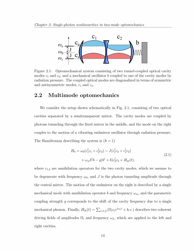
Figure 2.1: Optomechanical system consisting of two tunnel-coupled optical cavitymodes c1 and c2, and a mechanical oscillator b coupled to one of the cavity modes byradiation pressure. The coupled optical modes are diagonalized in terms of symmetricand antisymmetric modes, cs and ca.
2.2 Multimode optomechanics
We consider the setup shown schematically in Fig. 2.1, consisting of two optical
cavities separated by a semitransparent mirror. The cavity modes are coupled by
photons tunneling through the fixed mirror in the middle, and the mode on the right
couples to the motion of a vibrating endmirror oscillator through radiation pressure.
The Hamiltonian describing the system is (~ = 1)
H0 = ω0(c†1c1 + c†2c2)− J(c†1c2 + c†1c2)
+ ωmb†b− g(b† + b)c†2c2 +Hdr(t),
(2.1)
where c1,2 are annihilation operators for the two cavity modes, which we assume to
be degenerate with frequency ω0, and J is the photon tunneling amplitude through
the central mirror. The motion of the endmirror on the right is described by a single
mechanical mode with annihilation operator b and frequency ωm, and the parametric
coupling strength g corresponds to the shift of the cavity frequency due to a single
mechanical phonon. Finally, Hdr(t) =∑
i=1,2 (ΩicieiωLt + h.c.) describes two coherent
driving fields of amplitudes Ωi and frequency ωL, which are applied to the left and
right cavities.
14
Chapter 2: Single-photon nonlinearities in two-mode optomechanics
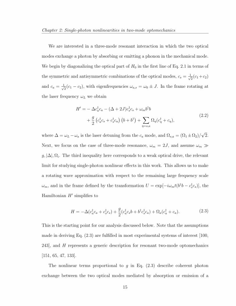
We are interested in a three-mode resonant interaction in which the two optical
modes exchange a photon by absorbing or emitting a phonon in the mechanical mode.
We begin by diagonalizing the optical part of H0 in the first line of Eq. 2.1 in terms of
the symmetric and antisymmetric combinations of the optical modes, cs = 1√2(c1 +c2)
and ca = 1√2(c1 − c2), with eigenfrequencies ωa,s = ω0 ± J . In the frame rotating at
the laser frequency ωL we obtain
H ′ =−∆c†aca − (∆ + 2J)c†scs + ωmb†b
+g
2
(c†acs + c†sca
) (b+ b†
)+∑
η=s,a
Ωη(c†η + cη),
(2.2)
where ∆ = ωL−ωa is the laser detuning from the ca mode, and Ωs,a = (Ω1±Ω2)/√
2.
Next, we focus on the case of three-mode resonance, ωm = 2J , and assume ωm
g, |∆|,Ωi. The third inequality here corresponds to a weak optical drive, the relevant
limit for studying single-photon nonlinear effects in this work. This allows us to make
a rotating wave approximation with respect to the remaining large frequency scale
ωm, and in the frame defined by the transformation U = exp[−iωmt(b†b− c†scs)], the
Hamiltonian H ′ simplifies to
H = −∆(c†aca + c†scs) +g
2(c†acsb+ b†c†sca) + Ωa(c
†a + ca). (2.3)
This is the starting point for our analysis discussed below. Note that the assumptions
made in deriving Eq. (2.3) are fulfilled in most experimental systems of interest [100,
243], and H represents a generic description for resonant two-mode optomechanics
[151, 65, 47, 133].
The nonlinear terms proportional to g in Eq. (2.3) describe coherent photon
exchange between the two optical modes mediated by absorption or emission of a
15
Chapter 2: Single-photon nonlinearities in two-mode optomechanics
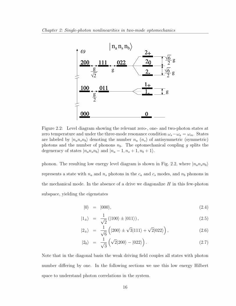
Figure 2.2: Level diagram showing the relevant zero-, one- and two-photon states atzero temperature and under the three-mode resonance condition ωs−ωa = ωm. Statesare labeled by |nansnb〉 denoting the number na (ns) of antisymmetric (symmetric)photons and the number of phonons nb. The optomechanical coupling g splits thedegeneracy of states |nansnb〉 and |na − 1, ns + 1, nb + 1〉.
phonon. The resulting low energy level diagram is shown in Fig. 2.2, where |nansnb〉
represents a state with na and ns photons in the ca and cs modes, and nb phonons in
the mechanical mode. In the absence of a drive we diagonalize H in this few-photon
subspace, yielding the eigenstates
|0〉 = |000〉, (2.4)
|1±〉 =1√2
(|100〉 ± |011〉) , (2.5)
|2±〉 =1√6
(|200〉 ±
√3|111〉+
√2|022〉
), (2.6)
|20〉 =1√3
(√2|200〉 − |022〉
). (2.7)
Note that in the diagonal basis the weak driving field couples all states with photon
number differing by one. In the following sections we use this low energy Hilbert
space to understand photon correlations in the system.
16
Chapter 2: Single-photon nonlinearities in two-mode optomechanics
In addition to the coherent evolution modeled by the Hamiltonian H, we describe
optical and mechanical dissipation using a master equation for the system density
operator ρ,
ρ = −i[H, ρ] + κD[ca]ρ+ κD[cs]ρ (2.8)
+γ
2(Nth + 1)D[b]ρ+
γ
2NthD[b†]ρ, (2.9)
where H is given by Eq. 2.3, 2κ and γ are energy decay rates for the optical and
mechanical modes, respectively, Nth is the thermal phonon population and D[o]ρ =
2oρo† − o†oρ− ρo†o. Below we study nonlinear effects at the level of single photons,
both numerically and analytically, by solving Eq. 2.8 approximately in the limit of
weak optical driving, Ω ≡ Ωa κ.
2.3 Equal-time correlations
2.3.1 Average transmission and reflection
Before focusing on photon-photon correlations, we first study the average trans-
mission through the cavity, which is proportional to the mean intracavity photon
number. In Fig. 2.3 and 2.4 we show the intracavity photon number of the two
optical modes,
ni =⟨c†ici
⟩, (2.10)
where i = a, s, and angle brackets denote the steady state average. At ∆/g = ±12,
both transmission curves exhibit a maximum, indicating that the driving field is
in resonance with an eigenmode of the system. The position of these peaks can
17
Chapter 2: Single-photon nonlinearities in two-mode optomechanics
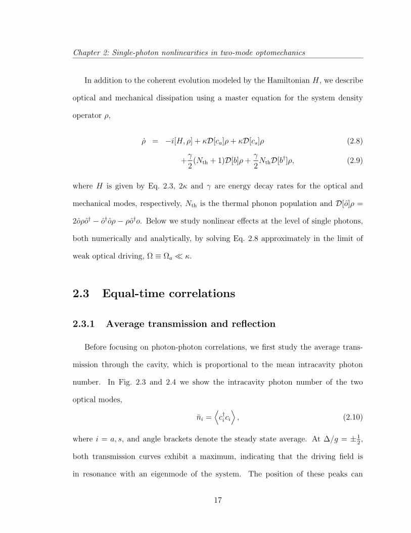
Figure 2.3: Normalized average photon number (green “+”) and photon-photoncorrelation function (blue “”) for driven mode ca as a function of laser detuning atzero temperature. Solid lines are calculated from analytic model (see Eqs. (2.19-2.24))and points show full numerical calculation. The average photon number is normalizedby n0 = (Ω/κ)2. (g/κ = 20 and γ/κ = 0.2)
be understood from the level diagram shown in Fig. 2.2, which at finite g shows a
splitting of the lowest photonic states into a doublet, |1±〉 = (|100〉 ± |011〉)/√
2.
In addition to the transmission, we plot the mean reflected photon number in
Fig. 2.5. As discussed below, the reflected photon statistics can also exhibit signatures
of nonlinearity. We calculate properties of the reflected light using the annihilation
operator cR = ca+iΩκ
, obtained from standard input-output relations for a symmetric
two-sided cavity (see Appendix A.1). The mean reflected photon number nR =⟨c†RcR
⟩is plotted in Fig. 2.5. At ∆/g = ±1
2, the average reflection has a minimum
where the average transmission has a maximum. Note that in contrast to a single
cavity, even on resonance the transmission probability is less than unity and the
reflection probability remains finite.
18
Chapter 2: Single-photon nonlinearities in two-mode optomechanics
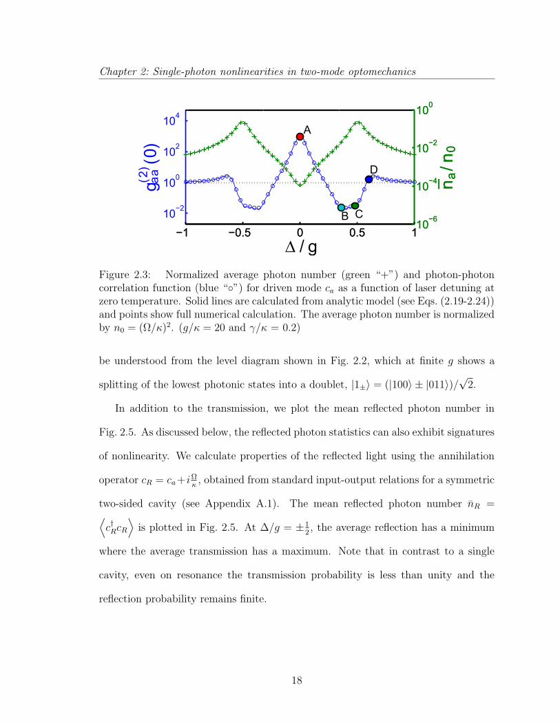
Figure 2.4: Normalized average photon number (green “+”) and photon-photoncorrelation function (blue “”) for the undriven mode cs as a function of laser detuningat zero temperature. Solid lines are calculated from analytic model (see Eqs. (2.19-2.24)) and points show full numerical calculation. The average photon number isnormalized by n0 = (Ω/κ)2. (g/κ = 20 and γ/κ = 0.2)
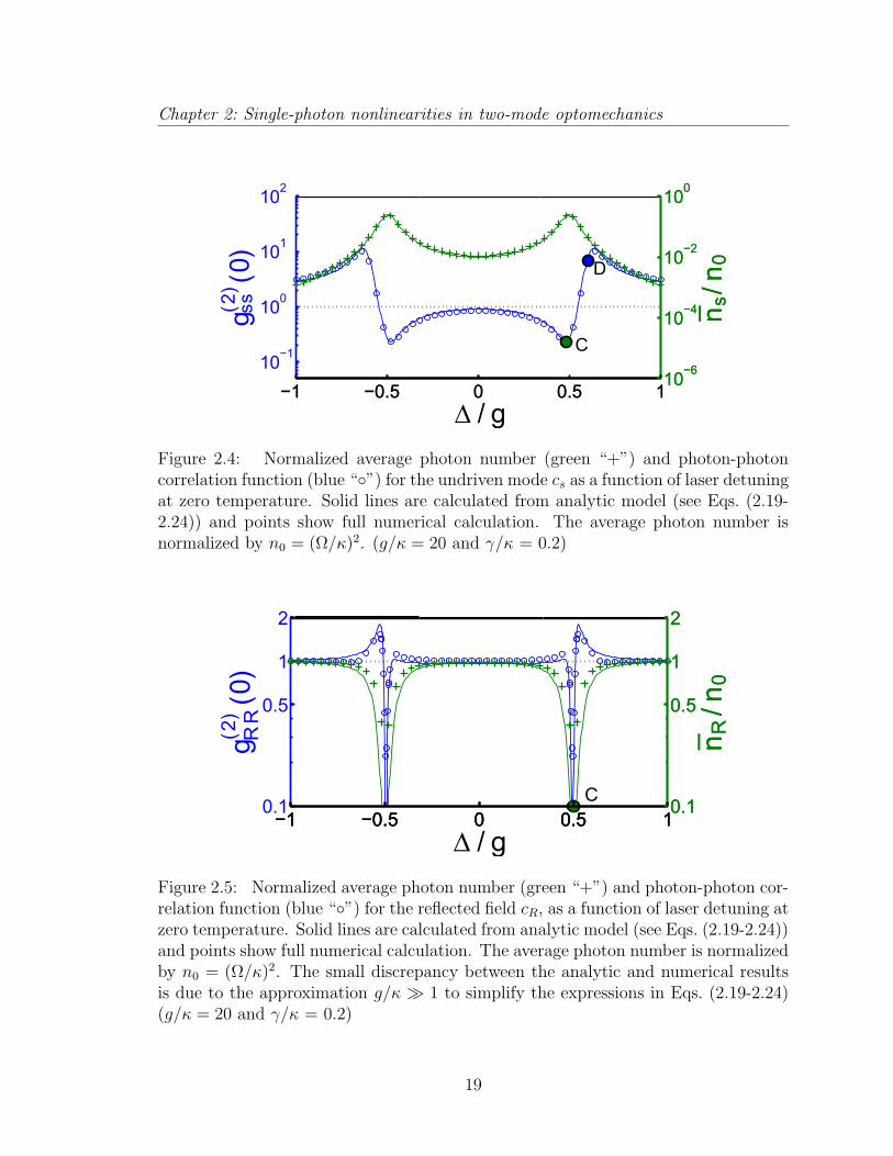
Figure 2.5: Normalized average photon number (green “+”) and photon-photon cor-relation function (blue “”) for the reflected field cR, as a function of laser detuning atzero temperature. Solid lines are calculated from analytic model (see Eqs. (2.19-2.24))and points show full numerical calculation. The average photon number is normalizedby n0 = (Ω/κ)2. The small discrepancy between the analytic and numerical resultsis due to the approximation g/κ 1 to simplify the expressions in Eqs. (2.19-2.24)(g/κ = 20 and γ/κ = 0.2)
19
Chapter 2: Single-photon nonlinearities in two-mode optomechanics
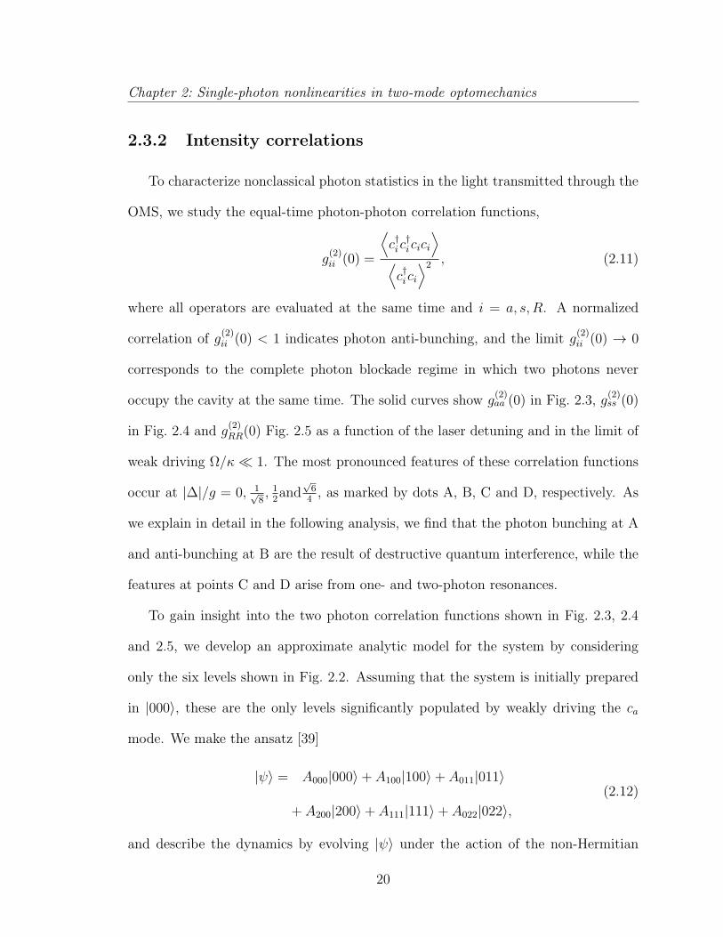
2.3.2 Intensity correlations
To characterize nonclassical photon statistics in the light transmitted through the
OMS, we study the equal-time photon-photon correlation functions,
g(2)ii (0) =
⟨c†ic†icici
⟩
⟨c†ici
⟩2 , (2.11)
where all operators are evaluated at the same time and i = a, s, R. A normalized
correlation of g(2)ii (0) < 1 indicates photon anti-bunching, and the limit g
(2)ii (0) → 0
corresponds to the complete photon blockade regime in which two photons never
occupy the cavity at the same time. The solid curves show g(2)aa (0) in Fig. 2.3, g
(2)ss (0)
in Fig. 2.4 and g(2)RR(0) Fig. 2.5 as a function of the laser detuning and in the limit of
weak driving Ω/κ 1. The most pronounced features of these correlation functions
occur at |∆|/g = 0, 1√8, 1
2and
√6
4, as marked by dots A, B, C and D, respectively. As
we explain in detail in the following analysis, we find that the photon bunching at A
and anti-bunching at B are the result of destructive quantum interference, while the
features at points C and D arise from one- and two-photon resonances.
To gain insight into the two photon correlation functions shown in Fig. 2.3, 2.4
and 2.5, we develop an approximate analytic model for the system by considering
only the six levels shown in Fig. 2.2. Assuming that the system is initially prepared
in |000〉, these are the only levels significantly populated by weakly driving the ca
mode. We make the ansatz [39]
|ψ〉 = A000|000〉+ A100|100〉+ A011|011〉
+ A200|200〉+ A111|111〉+ A022|022〉,(2.12)
and describe the dynamics by evolving |ψ〉 under the action of the non-Hermitian
20

Chapter 2: Single-photon nonlinearities in two-mode optomechanics
Hamiltonian, H = H − i[κc†aca + κc†scs + γ
2b†b]. This approach allows us to evaluate
intensities up to order Ω2 and two-point correlation up to order Ω4, since the neglected
quantum jumps lead to higher order corrections. By neglecting the typically small
mechanical decay rate γ κ, the amplitudes in Eq. 2.12 then satisfy
A000 = 0, (2.13)
A100 = −ig2A011 − iΩA000 − κA100, (2.14)
A011 = −ig2A100 − κA011, (2.15)
A200 = −i g√2A111 − i
√2ΩA100 − 2κA200, (2.16)
A111 = −i g√2A200 − igA022 − iΩA011 − 2κA111, (2.17)
A022 = −igA111 − 2κA022, (2.18)
where κ = κ − i∆. It is straightforward to solve Eqs. (2.13–2.18) for the steady
state amplitudes (see Appendix A.2). To lowest order in Ω/κ the mean occupation
numbers are na = |A100|2, ns = |A011|2 and nR = |A100 + iΩ/κ|2, where A denote
steady state amplitudes. We obtain
nan0
=κ2 [Rκ(0)]1/2
Rκ
(g2
) , (2.19)
nsn0
=g2κ2
4Rκ
(g2
) , (2.20)
nRn0
≈[Rκ/2
(g2
)]2[Rκ
(g2
)]2 , (2.21)
where RK(ω) = [K2 + (∆− ω)2] [K2 + (∆ + ω)2] and n0 = (Ω/κ)2. From the factors
RK(ω) in the denominators (numerators) in these expressions, we obtain the positions
of the resonances (antiresonances) in the average intracavity photon numbers, in
21
Chapter 2: Single-photon nonlinearities in two-mode optomechanics
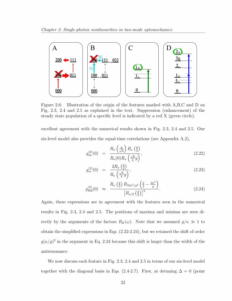
Figure 2.6: Illustration of the origin of the features marked with A,B,C and D onFig. 2.3, 2.4 and 2.5 as explained in the text. Suppression (enhancement) of thesteady state population of a specific level is indicated by a red X (green circle).
excellent agreement with the numerical results shown in Fig. 2.3, 2.4 and 2.5. Our
six-level model also provides the equal-time correlations (see Appendix A.2),
g(2)aa (0) =
Rκ
(g√8
)Rκ
(g2
)
Rκ(0)Rκ
(√6
4g) , (2.22)
g(2)ss (0) =
2Rκ
(g2
)
Rκ
(√6
4g) , (2.23)
g(2)RR(0) ≈
Rκ
(g2
)R16κ3/g2
(g2− 2κ2
g
)
[Rκ/2
(g2
)]2 . (2.24)
Again, these expressions are in agreement with the features seen in the numerical
results in Fig. 2.3, 2.4 and 2.5. The positions of maxima and minima are seen di-
rectly by the arguments of the factors RK(ω). Note that we assumed g/κ 1 to
obtain the simplified expressions in Eqs. (2.22-2.24), but we retained the shift of order
g(κ/g)2 in the argument in Eq. 2.24 because this shift is larger than the width of the
antiresonance.
We now discuss each feature in Fig. 2.3, 2.4 and 2.5 in terms of our six-level model
together with the diagonal basis in Eqs. (2.4-2.7). First, at detuning ∆ = 0 (point
22
Chapter 2: Single-photon nonlinearities in two-mode optomechanics
A in Fig. 2.3) we see g(2)aa (0) > 1, indicating bunching. This is due to destructive
interference that suppresses the population in |100〉 (panel A in Fig. 2.6), and can
be understood as the system being driven into a dark state, |d〉 ∝ g|000〉 − Ω|011〉,
similar to electromagnetically induced transparency (EIT) [134, 234]. In the dark
state, |011〉 remains populated, allowing transitions to |111〉 which in turn is strongly
coupled to |200〉. The net result is a relative suppression of the probability to have one
photon compared to two photons in the driven mode, leading to bunching at ∆ = 0.
Second, at detuning ∆ = g/√
8 (point B), mode ca shows anti-bunching due to a
suppressed two-photon probability. Again, this is due to destructive interference, or
the presence of a dark state in which |200〉 remains unpopulated (panel B). Third, at
detuning ∆ = g2
(point C), all modes show anti-bunching. This is due to a one-photon
resonant transition |0〉 → |1+〉 (panel C). Finally, at detuning ∆ =√
64g (point D),
both ca and cs show bunching due to a two-photon resonant transition |0〉 → |2+〉
(panel D).
2.3.3 Absence of two-photon resonance at ∆ = 0
At first glance, the level diagram in Fig. 2.2 together with bunching in Fig. 2.3
suggest a two-photon resonance at zero detuning ∆ = 0, where the energy of the
eigenstate |20〉 is equal to the energy of two drive photons. However, as discussed
above, the bunching at ∆ = 0 arises entirely from the suppression of a one-photon
population; further, we find that the expected two-photon resonance is cancelled by
interference. This can be seen from a second order perturbative calculation of the
two-photon Rabi frequency Ω(2)0,20
for the transition |0〉 → |20〉. The two-photon state
23
Chapter 2: Single-photon nonlinearities in two-mode optomechanics
|20〉 can be populated by the drive Hdr = Ω(c†a+ca) from state |0〉 via two intermediate
one-photon eigenstates, |1±〉 given by Eq. 2.5, with energies ω1± = −∆ ± g2
in the
rotating frame. The resulting Rabi frequency is
Ω(2)0,20
=∑
n=1−,1+
〈20|Hdr|n〉 〈n|Hdr|0〉ωn
, (2.25)
which vanishes at ∆ = 0 as a consequence of destructive interference between the two
amplitudes. The exact cancellation is lifted by including finite dissipation and the
full spectrum; nonetheless this simple argument shows that the expected two-photon
resonance at ∆ = 0 is strongly suppressed.
Further evidence of the absence of a two-photon resonance at ∆ = 0 is the lack of
bunching in the undriven mode in Fig. 2.4. If there were a two-photon resonance, one
would expect that bunching should also occur in the undriven mode, since the state
|20〉 involves both ca and cs modes. This is indeed the case at detuning ∆ =√
64g
(see point D in Fig. 2.4), where both modes show bunching as a result of two-photon
resonance. In contrast, we see no bunching in the undriven mode at ∆ = 0. This
supports our conclusion that the observed bunching at ∆ = 0 arises from suppression
of population in |100〉 due to interference, as discussed in Section 2.3.2, and not
from two-photon resonance. As discussed above, this interference does not suppress
population in |011〉, so we do not expect bunching in the cs mode from this effect.
Finally, to confirm our intuitive picture we plot the intensity correlation function,
g(2)tot(0) = 〈ntot(ntot − 1)〉 / 〈ntot〉2, of the total photon number, ntot = na + ns, in the
coupled OM system in Fig. 2.7. The probability to find one photon in the combined
cavity is maximal at ∆/g = ±12
due to one-photon resonance. Similarly, we observe
antibunching at point C and bunching at point D, due to interference and two-photon
24
Chapter 2: Single-photon nonlinearities in two-mode optomechanics
−1 −0.5 0 0.5 10.1
0.3
1
3
10
g(2)
tot(0)
∆/g
A
C
D
−1 −0.5 0 0.5 10.01
0.03
0.1
0.3
1
2ntot/n0
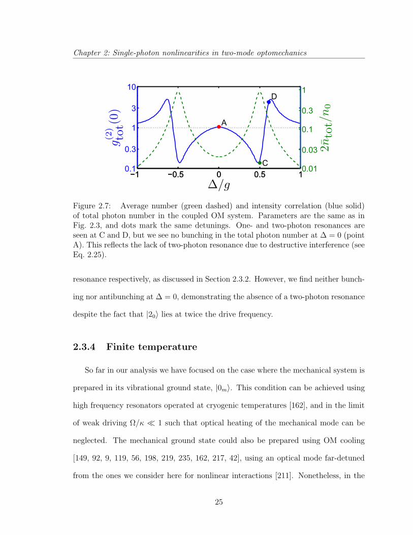
Figure 2.7: Average number (green dashed) and intensity correlation (blue solid)of total photon number in the coupled OM system. Parameters are the same as inFig. 2.3, and dots mark the same detunings. One- and two-photon resonances areseen at C and D, but we see no bunching in the total photon number at ∆ = 0 (pointA). This reflects the lack of two-photon resonance due to destructive interference (seeEq. 2.25).
resonance respectively, as discussed in Section 2.3.2. However, we find neither bunch-
ing nor antibunching at ∆ = 0, demonstrating the absence of a two-photon resonance
despite the fact that |20〉 lies at twice the drive frequency.
2.3.4 Finite temperature
So far in our analysis we have focused on the case where the mechanical system is
prepared in its vibrational ground state, |0m〉. This condition can be achieved using
high frequency resonators operated at cryogenic temperatures [162], and in the limit
of weak driving Ω/κ 1 such that optical heating of the mechanical mode can be
neglected. The mechanical ground state could also be prepared using OM cooling
[149, 92, 9, 119, 56, 198, 219, 235, 162, 217, 42], using an optical mode far-detuned
from the ones we consider here for nonlinear interactions [211]. Nonetheless, in the
25
Chapter 2: Single-photon nonlinearities in two-mode optomechanics
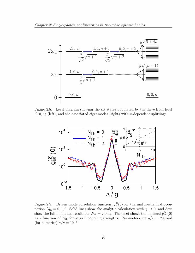
Figure 2.8: Level diagram showing the six states populated by the drive from level|0, 0, n〉 (left), and the associated eigenmodes (right) with n-dependent splittings.
Figure 2.9: Driven mode correlation function g(2)aa (0) for thermal mechanical occu-
pation Nth = 0, 1, 2. Solid lines show the analytic calculation with γ → 0, and dotsshow the full numerical results for Nth = 2 only. The inset shows the minimal g
(2)aa (0)
as a function of Nth for several coupling strengths. Parameters are g/κ = 20, and(for numerics) γ/κ = 10−3.
26
Chapter 2: Single-photon nonlinearities in two-mode optomechanics
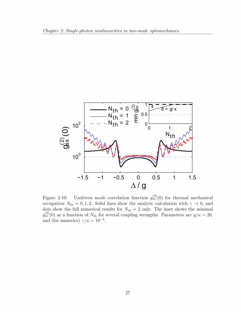
Figure 2.10: Undriven mode correlation function g(2)ss (0) for thermal mechanical
occupation Nth = 0, 1, 2. Solid lines show the analytic calculation with γ → 0, anddots show the full numerical results for Nth = 2 only. The inset shows the minimalg
(2)ss (0) as a function of Nth for several coupling strengths. Parameters are g/κ = 20,
and (for numerics) γ/κ = 10−3.
27
Chapter 2: Single-photon nonlinearities in two-mode optomechanics
following we extend our analytic treatment to the case of finite temperature, and
show that many of the nonclassical features are robust even in the presence of small
but finite thermal occupation of the mechanical mode.
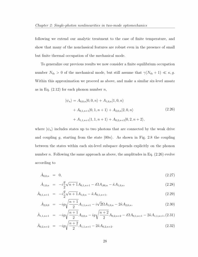
To generalize our previous results we now consider a finite equilibrium occupation
number Nth > 0 of the mechanical mode, but still assume that γ(Nth + 1) κ, g.
Within this approximation we proceed as above, and make a similar six-level ansatz
as in Eq. (2.12) for each phonon number n,
|ψn〉 = A0,0,n|0, 0, n〉+ A1,0,n|1, 0, n〉
+ A0,1,n+1|0, 1, n+ 1〉+ A2,0,n|2, 0, n〉
+ A1,1,n+1|1, 1, n+ 1〉+ A0,2,n+2|0, 2, n+ 2〉,
(2.26)
where |ψn〉 includes states up to two photons that are connected by the weak drive
and coupling g, starting from the state |00n〉. As shown in Fig. 2.8 the coupling
between the states within each six-level subspace depends explicitly on the phonon
number n. Following the same approach as above, the amplitudes in Eq. (2.26) evolve
according to
A0,0,n = 0, (2.27)
A1,0,n = −ig2
√n+ 1A0,1,n+1 − iΩA,00,n − κA1,0,n, (2.28)
A0,1,n+1 = −ig2
√n+ 1A1,0,n − κA0,1,n+1, (2.29)
A2,0,0 = −ig√n+ 1
2A1,1,n+1 − i
√2ΩA1,0,n − 2κA2,0,n, (2.30)
A1,1,n+1 = −ig√n+ 1
2A2,0,n − ig
√n+ 2
2A0,2,n+2 − iΩA0,1,n+1 − 2κA1,1,n+1,(2.31)
A0,2,n+2 = −ig√n+ 2
2A1,1,n+1 − 2κA0,2,n+2. (2.32)
28
Chapter 2: Single-photon nonlinearities in two-mode optomechanics
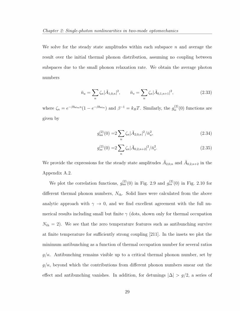
We solve for the steady state amplitudes within each subspace n and average the
result over the initial thermal phonon distribution, assuming no coupling between
subspaces due to the small phonon relaxation rate. We obtain the average photon
numbers
na =∑
n
ζn|A1,0,n|2, ns =∑
n
ζn|A0,1,n+1|2, (2.33)
where ζn = e−β~ωmn(1− e−β~ωm) and β−1 = kBT . Similarly, the g(2)ii (0) functions are
given by
g(2)aa (0) =2
∑
n
ζn|A2,0,n|2/n2a, (2.34)
g(2)ss (0) =2
∑
n
ζn|A0,2,n+2|2/n2s. (2.35)
We provide the expressions for the steady state amplitudes A2,0,n and A0,2,n+2 in the
Appendix A.2.
We plot the correlation functions, g(2)aa (0) in Fig. 2.9 and g
(2)ss (0) in Fig. 2.10 for
different thermal phonon numbers, Nth. Solid lines were calculated from the above
analytic approach with γ → 0, and we find excellent agreement with the full nu-
merical results including small but finite γ (dots, shown only for thermal occupation
Nth = 2). We see that the zero temperature features such as antibunching survive
at finite temperature for sufficiently strong coupling [211]. In the insets we plot the
minimum antibunching as a function of thermal occupation number for several ratios
g/κ. Antibunching remains visible up to a critical thermal phonon number, set by
g/κ, beyond which the contributions from different phonon numbers smear out the
effect and antibunching vanishes. In addition, for detunings |∆| > g/2, a series of
29
Chapter 2: Single-photon nonlinearities in two-mode optomechanics
new resonances appear in the correlation functions, and for small but finite occupa-
tion numbers we find new antibunching features that are absent for Nth = 0. These
new features can be understood from the n-dependent splitting of the one- and two-
photon manifolds as indicated in Fig. 2.8. For higher temperatures the individual
resonances start to overlap, and we observe an overall increase over a broad region of
large positive and negative detunings due to the cumulative effect of different phonon
numbers.
2.4 Delayed coincidence and single phonon states
In addition to the equal-time correlations discussed above, quantum signatures can
also be manifested in photon intensity correlations with a finite time delay. We now
turn to a discussion of delayed coincidence characterized by the two-time intensity
correlations functions,
g(2)ii (τ) =
⟨c†i (0)c†i (τ)ci(τ)ci(0)
⟩
⟨c†ici
⟩2 , (2.36)
for both driven and undriven modes, i = a, s. Expressing this correlation in terms
of a classical light intensity I, g(2)(τ) = 〈I(τ)I(0)〉 / 〈I〉2, and using the Schwarz
inequality, we obtain the inequalities [39, 31],
g(2)(τ) ≤ g(2)(0), (2.37)
|g(2)(τ)− 1| ≤ |g(2)(0)− 1|. (2.38)
Similar to the classical inequality g(2)(0) > 1 at zero delay, violation of either of these
inequalities at finite delay is a signature of quantum light. We calculate the delayed
30
Chapter 2: Single-photon nonlinearities in two-mode optomechanics
coincidence correlation functions for both the driven and undriven modes.
2.4.1 Driven mode
The correlation function g(2)aa (τ) is shown in Fig. 2.11(a) for two values of the
detuning ∆. The most striking feature is the apparent vanishing of g(2)aa (τ) at several
values of τ when the detuning is ∆ = 0 (curve A in Fig. 2.11(a)). These are due to
Rabi oscillations at frequency g/2 following the detection of a photon. This vanishing
of the finite delay correlation function is reminiscent of wavefunction collapse that
occurs in a cavity containing an atomic ensemble [39], and while its origins are similar,
there are important differences as we now discuss.
We can understand the finite delay intensity correlations in terms of the simple
six-level model discussed in the previous section. We extend this model to describe
finite delay correlations by considering the effect of photodetection on the steady state
of the system. Detection of a photon in the driven mode projects the system onto
the conditional state [89],
|ψa〉 =ca|ψ〉||ca|ψ〉||
, (2.39)
where |ψ〉 is given by Eq. 2.12 with steady state amplitudes and || · || denotes normal-
ization after the jump. The conditional state |ψa〉 has an increased amplitude A100
after the jump (see jump at τ = 0 in Fig. 2.11 (b)). Following this initial photode-
tection, the amplitude A100 subsequently undergoes Rabi oscillations with frequency
g/2, and decays back to its steady state at rate 2κ. For sufficiently large bunching at
zero delay and strong coupling g > κ, the Rabi oscillations of the amplitude A100(τ)
can cause it to cross zero several times before it decays back to steady state. As the
31
Chapter 2: Single-photon nonlinearities in two-mode optomechanics
probability to detect a second photon is dominated by A100, its zeros are responsible
for the zeros in the correlation function g(2)aa (τ) zero at these delay times.
The zeros in g(2)(τ) appear similar to those exhibited in a cavity strongly coupled
to an atomic ensemble [39, 179, 31] or a single atom [45]. However, in stark contrast to
the atomic case, the zeros in Fig. 2.11(a) are the result of Rabi oscillations following
the initial quantum jump. This is qualitatively different from the atomic case, where
the change in sign of the relevant amplitude (the analogy of A100) occurs immediately
after the jump itself, and the amplitude is damped back to steady state at the atomic
decay rate Γ, without Rabi oscillation. As a consequence, the vanishing correlation
function in the atomic case occurs at a delay set by τ0 ∼ γ−1 lnC, requiring only
strong cooperativity C = g2/κγ > 1 to be visible. On the other hand, the zeros in
Fig. 2.11(a) occur at delay times set by τ ∼ 1/g, requiring strictly strong coupling
g > κ.
Before moving on to correlations of the undriven mode, we briefly discuss the
correlations of the driven mode at the other value of detuning shown in Fig. 2.11(a).
At detuning ∆ = g√2
(curve E), which shows bunching at zero time, g(2)aa (0) & 1,
increases above its initial value at finite delay. This is a violation of the classical
inequality in Eq. 2.37, and is an example of “delayed bunching,” or an increased
probability to detect a second photon at a finite delay time. A similar effect was
recently studied in a single mode OMS [122]. However, like the Rabi oscillations,
the increased correlation function decays back to its steady state value of 1 on the
timescale of κ−1.
32
Chapter 2: Single-photon nonlinearities in two-mode optomechanics
0 5 10 15 20 25 30 350
1
2
3
4
5A
E
(a)
τ2τ1 gτ
g(2)
aa(τ)
A: ∆/g = 0
E: ∆/g = 1/√2
−5 0 5 10 15 20 25 30−2
0
2
4
6
8
gτ
A100(τ)/A
100
(b)
τ2τ1
∆/g = 0
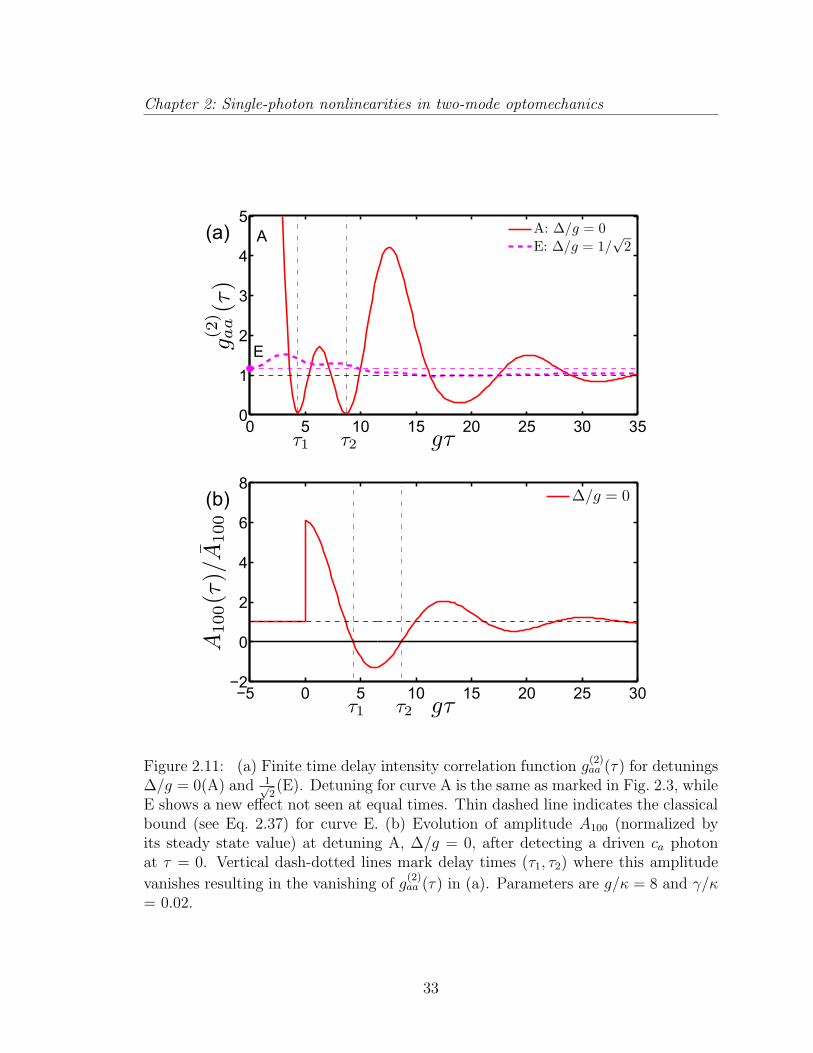
Figure 2.11: (a) Finite time delay intensity correlation function g(2)aa (τ) for detunings
∆/g = 0(A) and 1√2(E). Detuning for curve A is the same as marked in Fig. 2.3, while
E shows a new effect not seen at equal times. Thin dashed line indicates the classicalbound (see Eq. 2.37) for curve E. (b) Evolution of amplitude A100 (normalized byits steady state value) at detuning A, ∆/g = 0, after detecting a driven ca photonat τ = 0. Vertical dash-dotted lines mark delay times (τ1, τ2) where this amplitude
vanishes resulting in the vanishing of g(2)aa (τ) in (a). Parameters are g/κ = 8 and γ/κ
= 0.02.
33
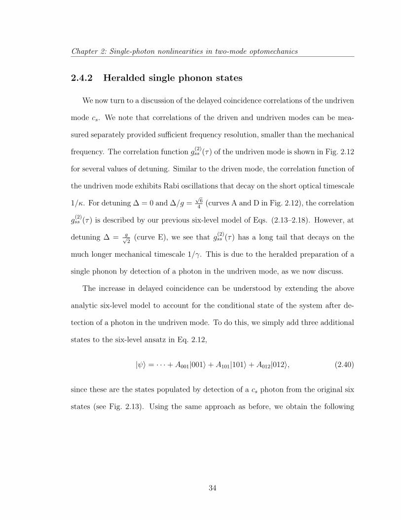
Chapter 2: Single-photon nonlinearities in two-mode optomechanics
2.4.2 Heralded single phonon states
We now turn to a discussion of the delayed coincidence correlations of the undriven
mode cs. We note that correlations of the driven and undriven modes can be mea-
sured separately provided sufficient frequency resolution, smaller than the mechanical
frequency. The correlation function g(2)ss (τ) of the undriven mode is shown in Fig. 2.12
for several values of detuning. Similar to the driven mode, the correlation function of
the undriven mode exhibits Rabi oscillations that decay on the short optical timescale
1/κ. For detuning ∆ = 0 and ∆/g =√
64
(curves A and D in Fig. 2.12), the correlation
g(2)ss (τ) is described by our previous six-level model of Eqs. (2.13–2.18). However, at
detuning ∆ = g√2
(curve E), we see that g(2)ss (τ) has a long tail that decays on the
much longer mechanical timescale 1/γ. This is due to the heralded preparation of a
single phonon by detection of a photon in the undriven mode, as we now discuss.
The increase in delayed coincidence can be understood by extending the above
analytic six-level model to account for the conditional state of the system after de-
tection of a photon in the undriven mode. To do this, we simply add three additional
states to the six-level ansatz in Eq. 2.12,
|ψ〉 = · · ·+ A001|001〉+ A101|101〉+ A012|012〉, (2.40)
since these are the states populated by detection of a cs photon from the original six
states (see Fig. 2.13). Using the same approach as before, we obtain the following
34
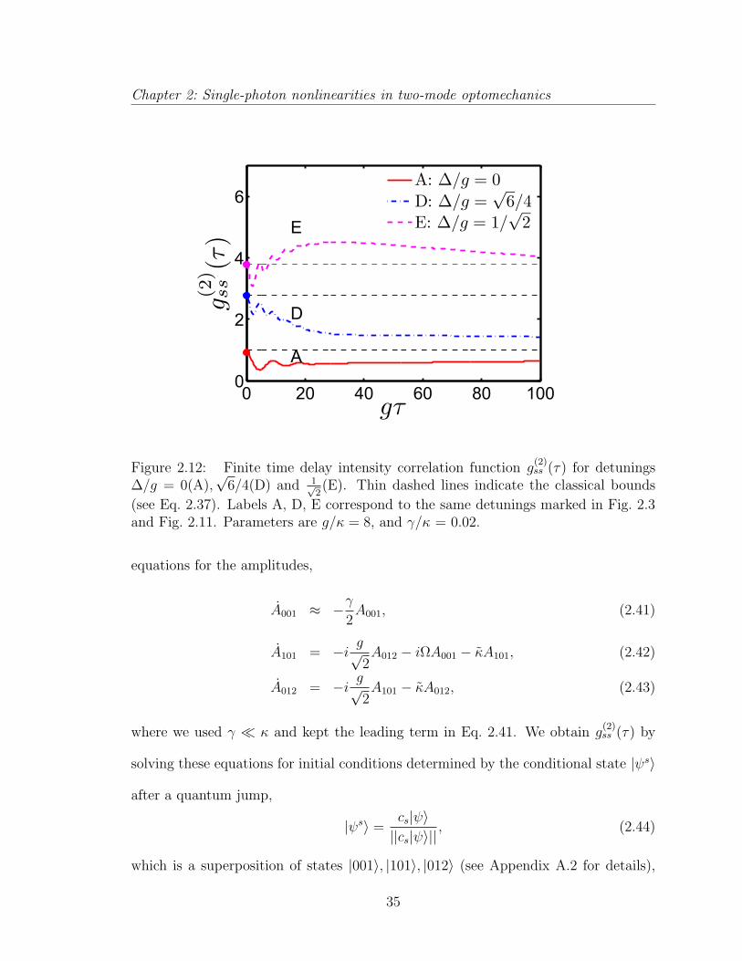
Chapter 2: Single-photon nonlinearities in two-mode optomechanics
0 20 40 60 80 1000
2
4
6
A
D
E
gτ
g(2)
ss(τ)
A: ∆/g = 0
D: ∆/g =√6/4
E: ∆/g = 1/√2
Figure 2.12: Finite time delay intensity correlation function g(2)ss (τ) for detunings
∆/g = 0(A),√
6/4(D) and 1√2(E). Thin dashed lines indicate the classical bounds
(see Eq. 2.37). Labels A, D, E correspond to the same detunings marked in Fig. 2.3and Fig. 2.11. Parameters are g/κ = 8, and γ/κ = 0.02.
equations for the amplitudes,
A001 ≈ −γ2A001, (2.41)
A101 = −i g√2A012 − iΩA001 − κA101, (2.42)
A012 = −i g√2A101 − κA012, (2.43)
where we used γ κ and kept the leading term in Eq. 2.41. We obtain g(2)ss (τ) by
solving these equations for initial conditions determined by the conditional state |ψs〉
after a quantum jump,
|ψs〉 =cs|ψ〉||cs|ψ〉||
, (2.44)
which is a superposition of states |001〉, |101〉, |012〉 (see Appendix A.2 for details),
35
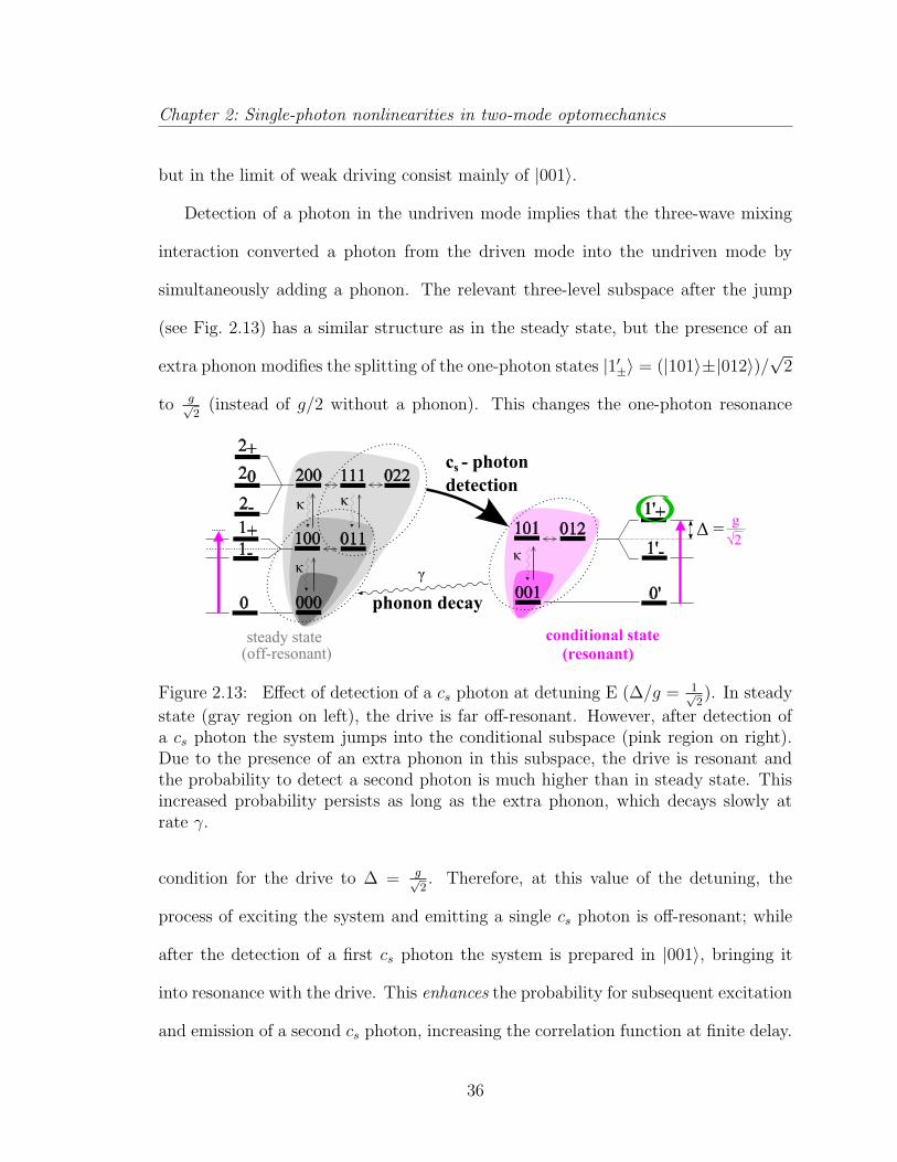
Chapter 2: Single-photon nonlinearities in two-mode optomechanics
but in the limit of weak driving consist mainly of |001〉.
Detection of a photon in the undriven mode implies that the three-wave mixing
interaction converted a photon from the driven mode into the undriven mode by
simultaneously adding a phonon. The relevant three-level subspace after the jump
(see Fig. 2.13) has a similar structure as in the steady state, but the presence of an
extra phonon modifies the splitting of the one-photon states |1′±〉 = (|101〉±|012〉)/√
2
to g√2
(instead of g/2 without a phonon). This changes the one-photon resonance
Figure 2.13: Effect of detection of a cs photon at detuning E (∆/g = 1√2). In steady
state (gray region on left), the drive is far off-resonant. However, after detection ofa cs photon the system jumps into the conditional subspace (pink region on right).Due to the presence of an extra phonon in this subspace, the drive is resonant andthe probability to detect a second photon is much higher than in steady state. Thisincreased probability persists as long as the extra phonon, which decays slowly atrate γ.
condition for the drive to ∆ = g√2. Therefore, at this value of the detuning, the
process of exciting the system and emitting a single cs photon is off-resonant; while
after the detection of a first cs photon the system is prepared in |001〉, bringing it
into resonance with the drive. This enhances the probability for subsequent excitation
and emission of a second cs photon, increasing the correlation function at finite delay.
36
Chapter 2: Single-photon nonlinearities in two-mode optomechanics
The maximum delayed coincidence occurs after a delay of τ ∼ 1/κ, when the photons
have reached the metastable steady state in the conditional subspace with one extra
phonon. Eventually, the delayed coincidence returns to its true steady state value of
one on the timescale τ ∼ 1/γ, which is the mechanical decay time of the state |001〉.
The long tails observed for other values of detuning (curves A and D) are also due to
the presence of an extra phonon, but in these cases the system remains off-resonant
after the initial cs photon and the effect is less pronounced. Note that the probability
to detect a photon from the driven mode also increases in the conditional state, so
a similar effect is seen in the delayed cross-correlation function g(2)as (τ), where the
photon in the undriven mode is detected first.
2.5 Reaching strong coupling
The nonclassical correlations predicted in this chapter require strong optomechan-
ical coupling, g > κ, as well as sideband resolution, ωm κ, γ. While the combina-
tion of these conditions has not yet been demonstrated, several experimental efforts
are currently directed at reaching this regime. By using micro- and nano-fabricated
OMSs such as microtoroids or photonic crystal beams, high frequency mechanical
systems with ωm ≈ 50 MHz - 5 GHz can be combined with low loss optical modes,
such that the condition ωm κ γ is satisfied [188, 198, 79]. At the same time
the mechanical system can already be prepared close to the quantum ground state
by working at cryogenic temperatures. In micro-fabricated OMSs, single-photon cou-
plings of about g/κ ≈ 0.001 have been demonstrated [79, 63, 230] The largest value
to date of g/κ ≈ 0.007 has been reached in photonic crystal beam resonators [43],
37
Chapter 2: Single-photon nonlinearities in two-mode optomechanics
where colocalized optical and vibrational resonances are highly confined to maximize
coupling while the surrounding structure is engineered to minimize loss. Conversely,
in cold atomic experiments the effective strong OM coupling regime has been reached
[170], while sideband resolution remains a challenge [210].
There are several existing proposals for how to meet the challenge of g/κ > 1 in the
photonic crystal beam setup. First, the single-photon optomechanical coupling can
be increased by making use of nanoslots in the structure [182, 58] to further localize
the electric field at the position of the mechanical mode. This could improve g by a
factor of 10 [133]. Second, numerical studies suggest that κ can be further decreased
by fine tuning the size and position of the slots in the photonic crystals [160, 213].
Finally, new materials are currently being tested for an overall improvement of the
OM properties of nano-fabricated devices [239]. Thus by using these ultrahigh Q
photonic crystals or similar designs, an increase of g/κ by a factor of ∼ 100 is realistic.
Note that once the strong coupling condition has been achieved, the implementation
of two or multimode OMSs with adjustable tunneling 2J ∼ ωm can be realized via
evanescent field coupling, as has already been demonstrated in the weak coupling
regime [188, 79, 100].
2.6 Conclusions
We have studied nonclassical intensity correlations in a driven, near-resonant op-
tomechanical system with one mechanical and two optical modes. In the regime of
strong coupling g > κ, this system allows for nonlinear quantum optics through a
resonant three-mode interaction in which the exchange of two photons is mediated by
38
Chapter 2: Single-photon nonlinearities in two-mode optomechanics
a phonon. We have identified several different processes that can lead to nonclassical
antibunching and delayed bunching, and we have derived a simple analytic model
that allows us to describe and interpret photon-photon correlations in this system
both at zero and at finite temperature. Our findings will be important as experi-
ments approach the regime of strong OM coupling, and for potential applications of
OMSs for quantum information processing. In particular, the long-lived correlation
found for the undriven mode raises the intriguing possibility to exploit such a setup
as a quantum memory. The generation of heralded single phonons on detection of
a photon from the undriven mode may have implications for building OM quantum
repeaters and quantum communication devices.
39

Chapter 3
Optomechanical quantum
information processing
3.1 Introduction
Optomechanics describes the radiation pressure interaction between an optical
cavity mode and the motion of a macroscopic mechanical object, as it appears, for
example, in a Fabry-Perot cavity with a moveable mirror [118, 142, 11]. First demon-
strations of optomechanical (OM) laser cooling [149, 92, 9, 119, 56, 219, 198, 235]
have recently attracted significant interest and led to tremendous progress in the
development of new fabrication methods and experimental techniques for controlling
OM interactions at the quantum level. Apart from ground-state cooling [217, 42], this
includes the demonstration of slow light [234, 187], and the coherent interconversion
of optical and mechanical excitations [86, 230]. These achievements pave the way for
a new type of quantum light-matter interface and give rise to interesting perspec-
40
Chapter 3: Optomechanical quantum information processing
tives for novel OM-based quantum technologies. As a solid-state approach, such an
all-OM platform would benefit directly from advanced nanofabrication and scalable
integrated photonic circuit techniques. At the same time, long mechanical lifetimes
comparable to those of atomic systems allow us to combine optical nonlinearities with
a stationary quantum memory for light.
In this work we study strong OM coupling effects in multimode OM systems
(OMSs) and describe how resonant or near-resonant interactions in this setting allow
us to exploit the intrinsic nonlinearity of radiation pressure in an optimal way. Our
approach is based on the resonant exchange of photons between two optical modes
mediated by a single phonon. This resonance induces much stronger nonlinearities
than achievable in single-mode OMSs, where nonlinear effects are suppressed by a
large mechanical frequency [143, 132, 171, 161]. Consequently, multimode OMSs
provide a promising route for accessing the single-photon strong-coupling regime,
where the coupling g0 as well as the mechanical frequency ωm exceeds the cavity decay
rate κ [171]. This regime is within reach of state-of-the-art nanoscale OM devices [42,
79, 40, 63] or analogous cold atom OMSs [101, 32], and here we discuss how strong
OM interactions in a multimode setup can be used to generate single photons and to
perform controlled gate operations between photonic or mechanical qubits. Combined
with very recently developed photon-phonon interfaces and quantum memories based
on linearized OM couplings [86, 230, 188], our results provide a basis for efficient OM
classical and quantum information processing with applications ranging from photon
transistors to quantum repeaters and networks.
41
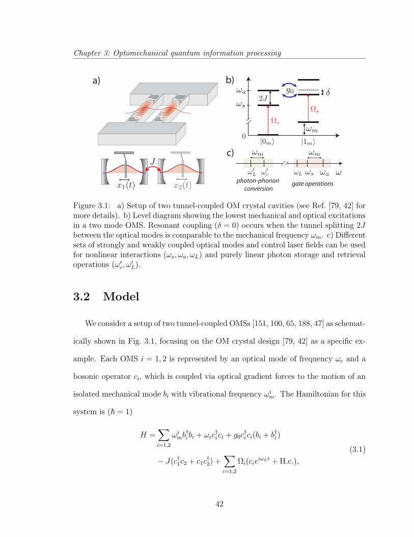
Chapter 3: Optomechanical quantum information processing
a) b)
photon-phonon conversion
gate operations
c)
Figure 3.1: a) Setup of two tunnel-coupled OM crystal cavities (see Ref. [79, 42] formore details). b) Level diagram showing the lowest mechanical and optical excitationsin a two mode OMS. Resonant coupling (δ = 0) occurs when the tunnel splitting 2Jbetween the optical modes is comparable to the mechanical frequency ωm. c) Differentsets of strongly and weakly coupled optical modes and control laser fields can be usedfor nonlinear interactions (ωs, ωa, ωL) and purely linear photon storage and retrievaloperations (ω′
c, ω′L).
3.2 Model
We consider a setup of two tunnel-coupled OMSs [151, 100, 65, 188, 47] as schemat-
ically shown in Fig. 3.1, focusing on the OM crystal design [79, 42] as a specific ex-
ample. Each OMS i = 1, 2 is represented by an optical mode of frequency ωc and a
bosonic operator ci, which is coupled via optical gradient forces to the motion of an
isolated mechanical mode bi with vibrational frequency ωim. The Hamiltonian for this
system is ( = 1)
H =∑
i=1,2
ωimb
†ibi + ωcc
†ici + g0c
†ici(bi + b†i )
− J(c†1c2 + c1c†2) +
∑
i=1,2
Ωi(cieiωLt +H.c.),
(3.1)
42
Chapter 3: Optomechanical quantum information processing
where J is the tunneling amplitude between the optical modes and g0 denotes the
single-photon OM coupling; Ωi are the local amplitudes of external control laser
fields of frequency ωL. Below we also consider an additional set of cavity modes and
driving fields with frequencies ω′c and ω′L, respectively. As indicated in Fig. 3.1(c), we
assume these modes to be separated in frequency and used for cooling the mechanical
modes [236, 141], and linear photon storage and retrieval operations [86, 230, 242, 2]
only.
Apart from the coherent dynamics described by Eq. (3.1), we include dissipation
through cavity decay and mechanical damping and model the evolution of the system
density operator ρ by a master equation (ME)
ρ =− i[H, ρ] +∑
i
κD[ci]ρ+ Lγρ, (3.2)
where D[c]ρ = 2cρc† − c†c, ρ+, and Lγ =∑
iγ2(Nth + 1)D[bi] + γ
2NthD[b†i ]. Here, κ
is the optical field decay rate, γ = ωm/Q the mechanical damping rate for a quality
factor Q and Nth = (e~ωm/kBT − 1)−1 the mechanical equilibrium occupation num-
ber for temperature T . Below we identify Γm = γ2(3Nth + 1
2) as the characteristic
decoherence rate for mechanical qubit states1.
3.3 Resonant strong-coupling optomechanics
We focus on the strong coupling regime ωm, g0 κ,Γm, and our main goal is
to show how the multimode OMS described by Eq. (3.1) can be used for imple-
menting controlled interactions between qubits encoded in photonic or phononic de-
1Γm corresponds to the initial decoherence rate of a phonon superposition (|0m〉+ |1m〉)/√
2.
43
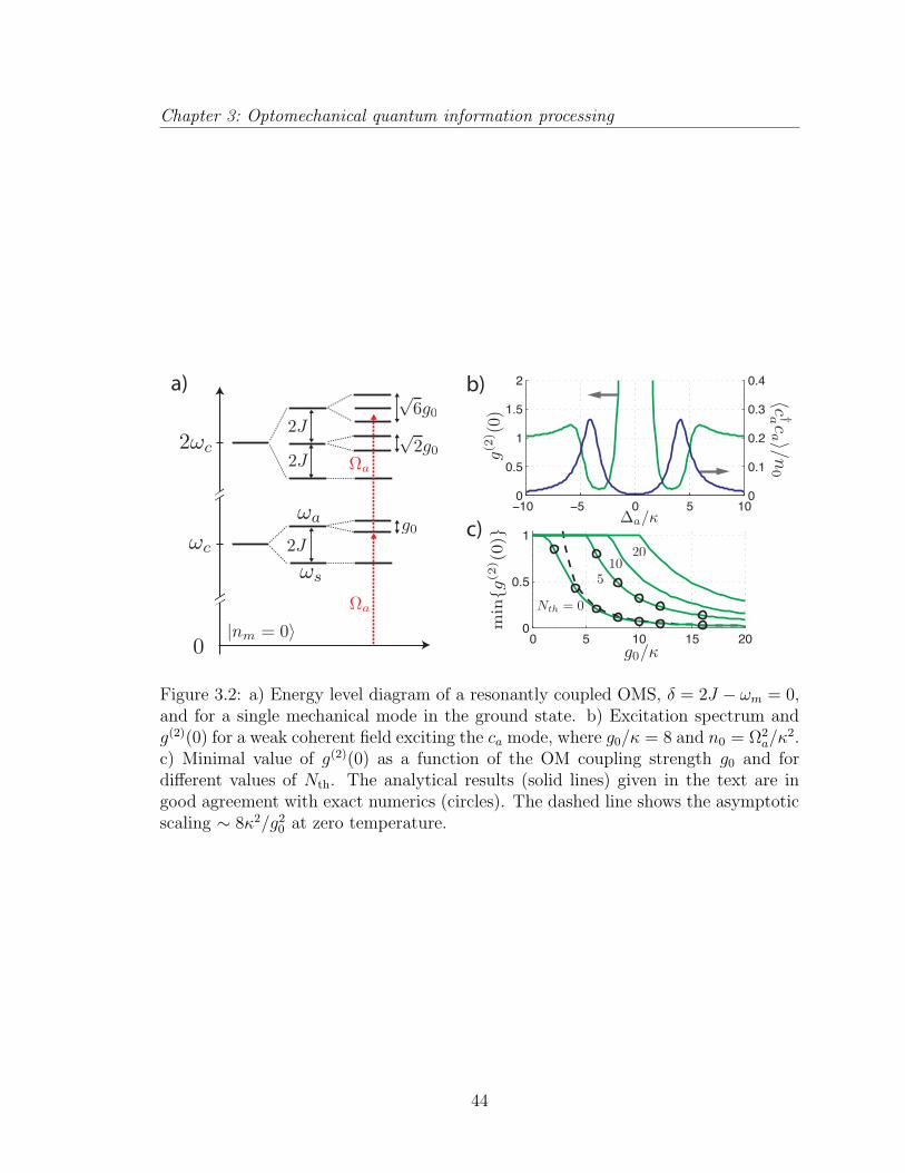
Chapter 3: Optomechanical quantum information processing
a) b)
c)
0 5 10 15 200
0.5
1
−10 −5 0 5 100
0.5
1
1.5
2
0
0.1
0.2
0.3
0.4
Figure 3.2: a) Energy level diagram of a resonantly coupled OMS, δ = 2J − ωm = 0,and for a single mechanical mode in the ground state. b) Excitation spectrum andg(2)(0) for a weak coherent field exciting the ca mode, where g0/κ = 8 and n0 = Ω2
a/κ2.
c) Minimal value of g(2)(0) as a function of the OM coupling strength g0 and fordifferent values of Nth. The analytical results (solid lines) given in the text are ingood agreement with exact numerics (circles). The dashed line shows the asymptoticscaling ∼ 8κ2/g2
0 at zero temperature.
44
Chapter 3: Optomechanical quantum information processing
grees of freedom. To illustrate this we first consider a single mechanical resonator,
b ≡ b1, ωm ≡ ω1m. We introduce symmetric and antisymmetric optical modes
cs,a = (c1 ± c2) /√
2 with eigenfrequencies ωs,a split by 2J . Further, we assume that
ωm ∼ 2J g0, κ, |δ|, where δ = 2J − ωm (see Fig. 3.1(b)). This condition can be
achieved in nanoscale OMSs where ωm ∼ GHz [79, 42, 40, 63] and a matching tunnel
splitting can be designed by appropriately adjusting the spacing between the cavi-
ties [79, 100]. In this regime we can make a rotating wave approximation with respect
to the large frequency scale ωm ∼ 2J and after changing into a frame rotating with
ωL we obtain [100]
H = −∆sc†scs −∆ac
†aca + ωmb
†b+g0
2(cac
†sb† + c†acsb) +HΩ(t). (3.3)
Here ∆s,a = ωL− ωs,a are the detunings of the driving field from the cs and ca mode,
respectively, and HΩ(t) =∑
η=s,a (Ωη(t)cη + H.c.) accounts for the external driving
fields with slowly varying amplitudes Ωs,a(t) = (Ω1(t)± Ω2(t))/√
2.
The two-mode OM coupling in Eq. (3.3) describes photon transitions between the
energetically higher mode ca to the lower mode cs, while simultaneously absorbing or
emitting a phonon. For (∆s −∆a − ωm) = δ = 0, this leads to a resonant interaction
between states |na, ns, nm〉 and |na− 1, ns + 1, nm + 1〉, where na, ns and nm label the
occupation numbers of the two optical modes and the mechanical mode, respectively.
In analogy to atomic cavity quantum electrodynamics (QED) [172], the nonlinear
scaling of the corresponding transition amplitudes g0
2
√na(ns + 1)(nm + 1) results in
an anharmonic level diagram as shown in Fig. 3.2(a). If g0 exceeds the cavity linewidth
κ, one and two photon transitions can be spectrally resolved, indicating the onset of
strong single-photon nonlinearities.
45
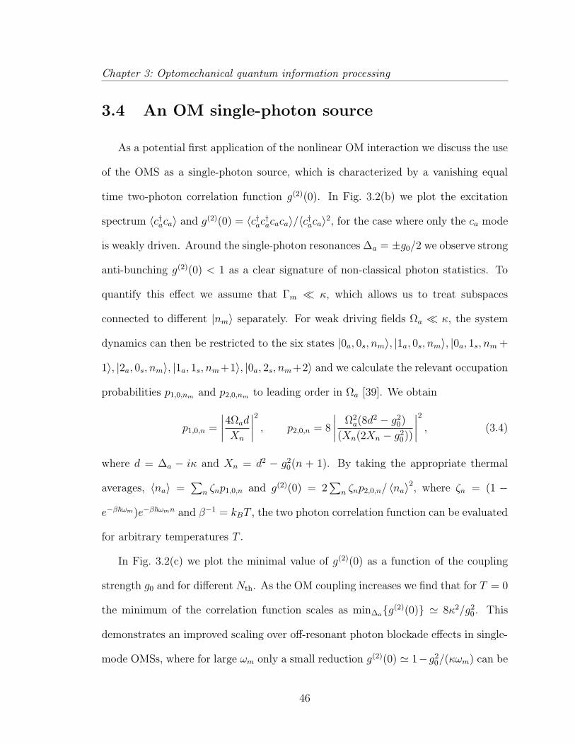
Chapter 3: Optomechanical quantum information processing
3.4 An OM single-photon source
As a potential first application of the nonlinear OM interaction we discuss the use
of the OMS as a single-photon source, which is characterized by a vanishing equal
time two-photon correlation function g(2)(0). In Fig. 3.2(b) we plot the excitation
spectrum 〈c†aca〉 and g(2)(0) = 〈c†ac†acaca〉/〈c†aca〉2, for the case where only the ca mode
is weakly driven. Around the single-photon resonances ∆a = ±g0/2 we observe strong
anti-bunching g(2)(0) < 1 as a clear signature of non-classical photon statistics. To
quantify this effect we assume that Γm κ, which allows us to treat subspaces
connected to different |nm〉 separately. For weak driving fields Ωa κ, the system
dynamics can then be restricted to the six states |0a, 0s, nm〉, |1a, 0s, nm〉, |0a, 1s, nm +
1〉, |2a, 0s, nm〉, |1a, 1s, nm+1〉, |0a, 2s, nm+2〉 and we calculate the relevant occupation
probabilities p1,0,nm and p2,0,nm to leading order in Ωa [39]. We obtain
p1,0,n =
∣∣∣∣4Ωad
Xn
∣∣∣∣2
, p2,0,n = 8
∣∣∣∣Ω2a(8d
2 − g20)
(Xn(2Xn − g20))
∣∣∣∣2
, (3.4)
where d = ∆a − iκ and Xn = d2 − g20(n + 1). By taking the appropriate thermal
averages, 〈na〉 =∑
n ζnp1,0,n and g(2)(0) = 2∑
n ζnp2,0,n/ 〈na〉2, where ζn = (1 −
e−β~ωm)e−β~ωmn and β−1 = kBT , the two photon correlation function can be evaluated
for arbitrary temperatures T .
In Fig. 3.2(c) we plot the minimal value of g(2)(0) as a function of the coupling
strength g0 and for different Nth. As the OM coupling increases we find that for T = 0
the minimum of the correlation function scales as min∆ag(2)(0) ' 8κ2/g20. This
demonstrates an improved scaling over off-resonant photon blockade effects in single-
mode OMSs, where for large ωm only a small reduction g(2)(0) ' 1−g20/(κωm) can be
46
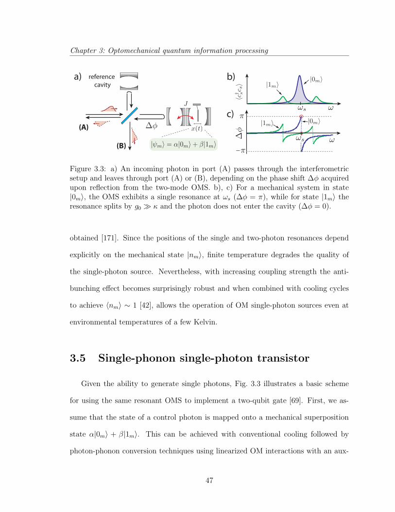
Chapter 3: Optomechanical quantum information processing
(A)
(B)
a) b)reference cavity
c)
Figure 3.3: a) An incoming photon in port (A) passes through the interferometricsetup and leaves through port (A) or (B), depending on the phase shift ∆φ acquiredupon reflection from the two-mode OMS. b), c) For a mechanical system in state|0m〉, the OMS exhibits a single resonance at ωs (∆φ = π), while for state |1m〉 theresonance splits by g0 κ and the photon does not enter the cavity (∆φ = 0).
obtained [171]. Since the positions of the single and two-photon resonances depend
explicitly on the mechanical state |nm〉, finite temperature degrades the quality of
the single-photon source. Nevertheless, with increasing coupling strength the anti-
bunching effect becomes surprisingly robust and when combined with cooling cycles
to achieve 〈nm〉 ∼ 1 [42], allows the operation of OM single-photon sources even at
environmental temperatures of a few Kelvin.
3.5 Single-phonon single-photon transistor
Given the ability to generate single photons, Fig. 3.3 illustrates a basic scheme
for using the same resonant OMS to implement a two-qubit gate [69]. First, we as-
sume that the state of a control photon is mapped onto a mechanical superposition
state α|0m〉 + β|1m〉. This can be achieved with conventional cooling followed by
photon-phonon conversion techniques using linearized OM interactions with an aux-
47
Chapter 3: Optomechanical quantum information processing
iliary mode ω′c (see Fig. 3.1(c)). Next, a single target photon of central frequency
∼ ωs is sent through the interferometric setup as described in Fig. 3.3. If the me-
chanical mode is in the state |0m〉, the incoming photon couples to a single resonant
state |0a, 1s, 0m〉 (see Fig. 3.1(b)), such that it enters the cavity and picks up a phase
before being reflected. Instead, if the mechanical resonator is in the state |1m〉, the
resonant coupling between |0a, 1s, 1m〉 and |1a, 0s, 0m〉 splits the cavity resonance, and
for g0 > κ the photon is reflected without a phase shift. Under ideal conditions, the
final result is an entangled state
|ψ〉 = α|0m, 1A, 0B〉+ β|1m, 0A, 1B〉, (3.5)
where A and B are the two ports of the interferometer. This state can be converted
back into an entangled state between the initial control and target photon.
Assuming that the storage and retrieval of the control photon can be achieved with
high fidelity, the error for producing the entangled state (3.5) with α = β = 1/√
2 is
approximately given by
ε ≈ 4κ2
g20
+1
(τpκ)2+ τpΓm, (3.6)
where τp is the duration of the single-photon pulse. The individual contributions in
Eq. (3.6) arise from an imperfect photon reflection, the finite spectral width of the
photon pulse, and mechanical decoherence, respectively. A minimal error is achieved
for τ−1p ≈ 3
√κ2Γm where we obtain ε ≈ max4κ2/g2
0,3√
Γ2m/κ
2. Assuming an OM
crystal device with ωm/(2π) = 4 GHz and Q = 105 as discussed in Ref. [42], but with
an improved OM coupling g0/(2π) = 50 MHz and a lower decay rate κ/(2π) = 5
MHz, we obtain gate errors ε ≈ 0.1 for environmental temperatures around T ≈ 100
mK.
48
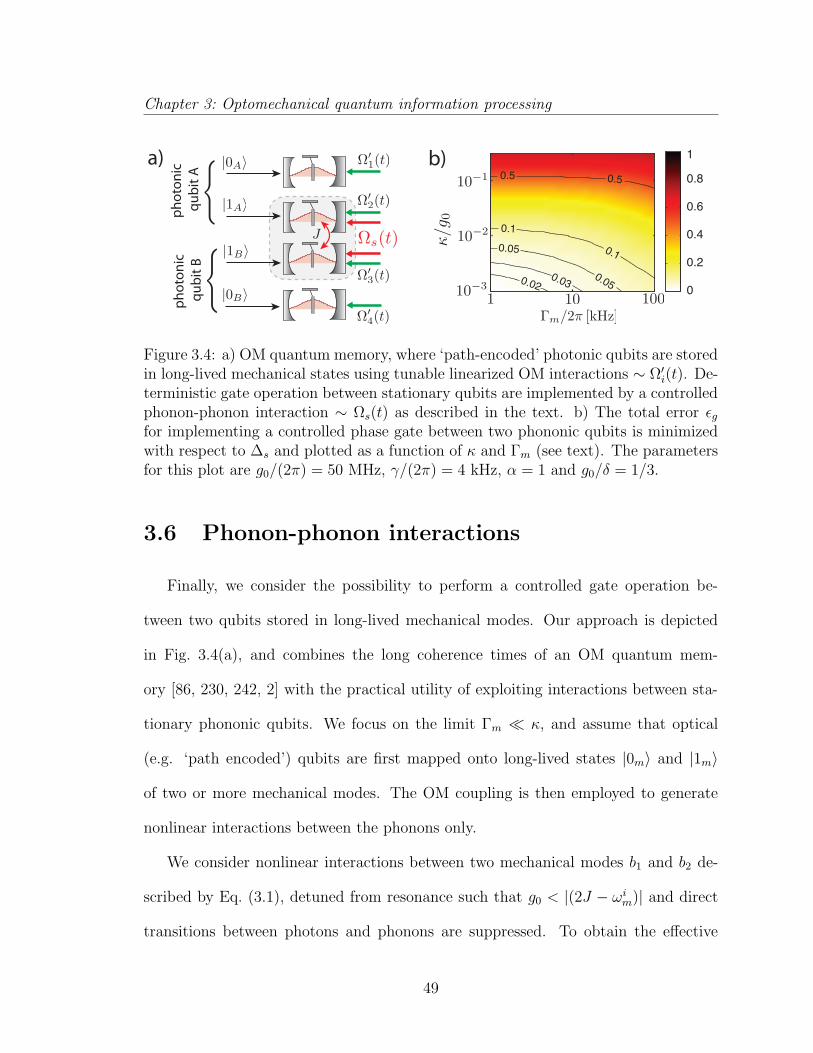
Chapter 3: Optomechanical quantum information processing
phot
onic
qu
bit A
phot
onic
qu
bit B
a) b)
0.020.03 0.05
0.05
0.1
0.1
0.5 0.5
0
0.2
0.4
0.6
0.8
1
Figure 3.4: a) OM quantum memory, where ‘path-encoded’ photonic qubits are storedin long-lived mechanical states using tunable linearized OM interactions ∼ Ω′i(t). De-terministic gate operation between stationary qubits are implemented by a controlledphonon-phonon interaction ∼ Ωs(t) as described in the text. b) The total error εgfor implementing a controlled phase gate between two phononic qubits is minimizedwith respect to ∆s and plotted as a function of κ and Γm (see text). The parametersfor this plot are g0/(2π) = 50 MHz, γ/(2π) = 4 kHz, α = 1 and g0/δ = 1/3.
3.6 Phonon-phonon interactions
Finally, we consider the possibility to perform a controlled gate operation be-
tween two qubits stored in long-lived mechanical modes. Our approach is depicted
in Fig. 3.4(a), and combines the long coherence times of an OM quantum mem-
ory [86, 230, 242, 2] with the practical utility of exploiting interactions between sta-
tionary phononic qubits. We focus on the limit Γm κ, and assume that optical
(e.g. ‘path encoded’) qubits are first mapped onto long-lived states |0m〉 and |1m〉
of two or more mechanical modes. The OM coupling is then employed to generate
nonlinear interactions between the phonons only.
We consider nonlinear interactions between two mechanical modes b1 and b2 de-
scribed by Eq. (3.1), detuned from resonance such that g0 < |(2J − ωim)| and direct
transitions between photons and phonons are suppressed. To obtain the effective
49
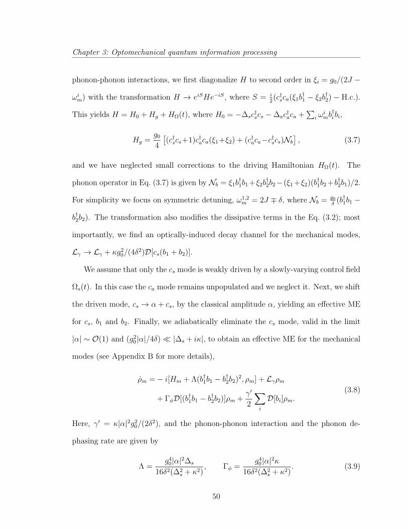
Chapter 3: Optomechanical quantum information processing
phonon-phonon interactions, we first diagonalize H to second order in ξi = g0/(2J −
ωim) with the transformation H → eiSHe−iS, where S = i2(c†sca(ξ1b
†1 − ξ2b
†2) − H.c.).
This yields H = H0 +Hg +HΩ(t), where H0 = −∆sc†scs −∆ac
†aca +
∑i ω
imb†ibi,
Hg =g0
4
[(c†scs+1)c†aca(ξ1+ξ2) + (c†aca−c†scs)Nb
], (3.7)
and we have neglected small corrections to the driving Hamiltonian HΩ(t). The
phonon operator in Eq. (3.7) is given by Nb = ξ1b†1b1 +ξ2b
†2b2−(ξ1 +ξ2)(b†1b2 +b†2b1)/2.
For simplicity we focus on symmetric detuning, ω1,2m = 2J ∓ δ, where Nb = g0
δ(b†1b1 −
b†2b2). The transformation also modifies the dissipative terms in the Eq. (3.2); most
importantly, we find an optically-induced decay channel for the mechanical modes,
Lγ → Lγ + κg20/(4δ
2)D[cs(b1 + b2)].
We assume that only the cs mode is weakly driven by a slowly-varying control field
Ωs(t). In this case the ca mode remains unpopulated and we neglect it. Next, we shift
the driven mode, cs → α+ cs, by the classical amplitude α, yielding an effective ME
for cs, b1 and b2. Finally, we adiabatically eliminate the cs mode, valid in the limit
|α| ∼ O(1) and (g20|α|/4δ) |∆s + iκ|, to obtain an effective ME for the mechanical
modes (see Appendix B for more details),
ρm =− i[Hm + Λ(b†1b1 − b†2b2)2, ρm] + Lγρm
+ ΓφD[(b†1b1 − b†2b2)]ρm +γ′
2
∑
i
D[bi]ρm.(3.8)
Here, γ′ = κ|α|2g20/(2δ
2), and the phonon-phonon interaction and the phonon de-
phasing rate are given by
Λ =g4
0|α|2∆s
16δ2(∆2s + κ2)
, Γφ =g4
0|α|2κ16δ2(∆2
s + κ2). (3.9)
50
Chapter 3: Optomechanical quantum information processing
The effective Hamiltonian in Eq. (3.8) describes a phonon nonlinearity with a tunable
strength Λ(t) ∼ |α(t)|2. The relevant cross-coupling is given by
Hint ' 2Λb†1b1b†2b2, (3.10)
and when acting for a time tg = π/(2Λ), this Hamiltonian implements a controlled-
phase gate between two qubits encoded in states |0m〉 and |1m〉. During this time,
phonons experience intrinsic and optically-induced decoherence as seen in Eq. (3.8).
In Fig. 3.4, we plot the resulting gate error εg = 1−〈ψ0|ρm(tg)|ψ0〉 for an initial state
|ψ0〉 = 12(|0m〉 + |1m〉)⊗2 optimized with respect to ∆s. Using the total decoherence
rate of this state, Γdecoh = 2Γm + Γφ + γ′/2, we find that εg ∝ Γdecoh/Λ is minimized
for |∆s| ' g0/2, where εg ∝ 4(κ/g0). While this scaling with g0 is weaker than for a
gate based on photon reflection (see Eq. (3.6)), the ability to perform a gate between
stationary qubits represents an important advantage of this approach.
3.7 Conclusions
We have described single-photon and single-phonon nonlinear effects in strongly
coupled multimode OMSs. We have shown how induced nonlinearities on or near
resonance can be used for controlled quantum gate operations between flying optical
or stationary phononic qubits. Our results provide a realistic route towards the
quantum nonlinear regime of OMSs, and a framework for future OM information
processing applications.
51
Chapter 4
Heralded Quantum Gates with
Integrated Error Detection
4.1 Introduction
Exploiting quantum systems for information processing offers many potential
advantages over classical information processing like highly secure quantum net-
works [54, 117, 70] and powerful quantum computers [124, 203, 85]. One of the
main challenges for the realization of functional quantum computers is to perform
gates with sufficiently high quality so that the remaining errors can be suppressed
by error correction codes, which makes the computation fault tolerant [120]. At the
same time, applications to long distance quantum communication can be enabled by
quantum repeaters, which combine probabilistic entanglement generation over short
distances with subsequent entanglement connection steps [70]. For these protocols,
the probabilistic nature of the entanglement generation is acceptable, but it is essential
52
Chapter 4: Heralded Quantum Gates with Integrated Error Detection
that high fidelity entanglement is achieved conditioned on a heralding measurement.
Experimentally, such high fidelity entanglement is often much easier to implement
and may be realized in situations where it is impossible to perform any quantum
operations deterministically. Here we introduce a similar concept for gate operations
and develop the concept of heralded quantum gates with integrated error detection.
In the resulting gate, the infidelity, which would be present for a deterministic gate
is converted into a failure probability, which is heralded by an auxiliary atom. Once
successful, the resulting gate can have an arbitrarily small error. Such heralded gates
could facilitate fault tolerant quantum computation since detectable errors may be
easier to correct than undetectable errors [98, 173, 229]. Alternatively it can be di-
rectly incorporated into quantum repeater architectures for long distance quantum
communication.
Optical cavities are ideal for conversion between the stationary gate qubits and
flying qubits (photons), which is fundamental for quantum networks [181, 121, 169].
Quantum gates can, in principle, also be directly implemented in optical cavities [168],
but the experimental requirements for this are very challenging due to spontaneous
emission and cavity loss. The essential parameter quantifying this is the coopera-
tivity of the atom-cavity system, C. It has been argued that directly implementing
gates in optical cavities leads to a poor error scaling 1 − F ∝ 1/√C, where F is
the fidelity of the gate [115, 208]. However, as a result of the integrated error detec-
tion, the heralded gates that we propose exhibit high fidelities when successful. This
enables efficient entanglement swapping and removes the necessity of intermediate
entanglement purification in quantum repeaters thus increasing the distribution rate
53
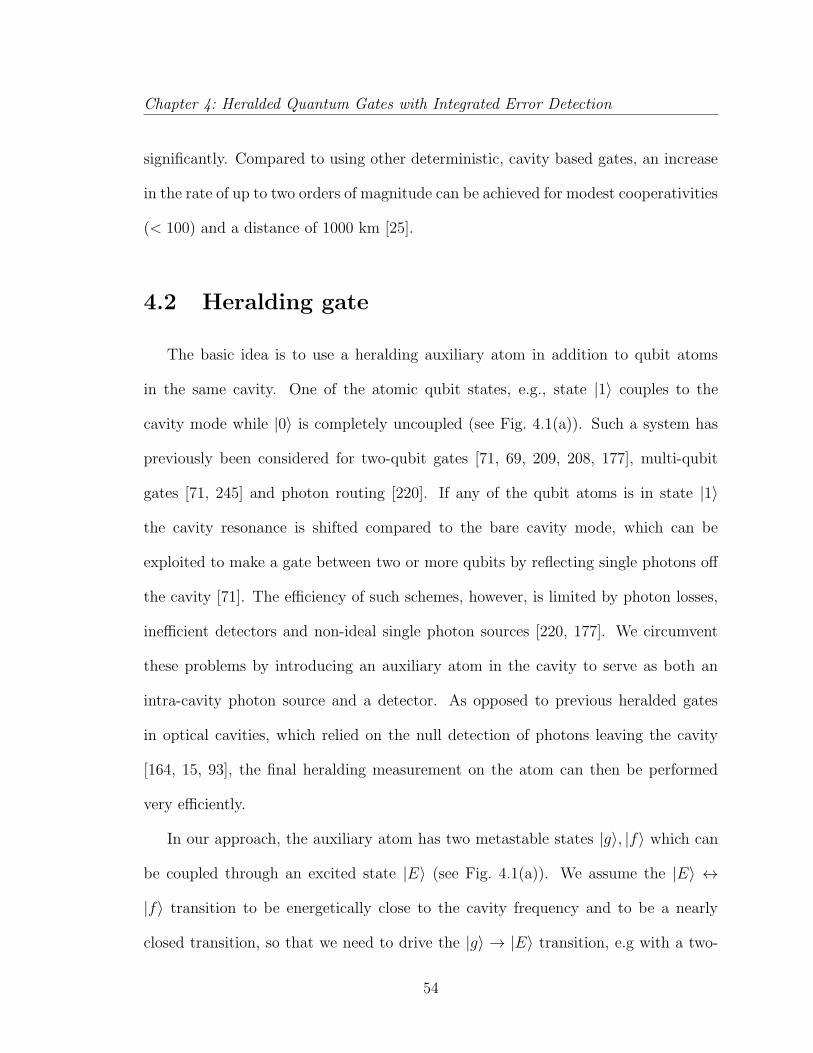
Chapter 4: Heralded Quantum Gates with Integrated Error Detection
significantly. Compared to using other deterministic, cavity based gates, an increase
in the rate of up to two orders of magnitude can be achieved for modest cooperativities
(< 100) and a distance of 1000 km [25].
4.2 Heralding gate
The basic idea is to use a heralding auxiliary atom in addition to qubit atoms
in the same cavity. One of the atomic qubit states, e.g., state |1〉 couples to the
cavity mode while |0〉 is completely uncoupled (see Fig. 4.1(a)). Such a system has
previously been considered for two-qubit gates [71, 69, 209, 208, 177], multi-qubit
gates [71, 245] and photon routing [220]. If any of the qubit atoms is in state |1〉
the cavity resonance is shifted compared to the bare cavity mode, which can be
exploited to make a gate between two or more qubits by reflecting single photons off
the cavity [71]. The efficiency of such schemes, however, is limited by photon losses,
inefficient detectors and non-ideal single photon sources [220, 177]. We circumvent
these problems by introducing an auxiliary atom in the cavity to serve as both an
intra-cavity photon source and a detector. As opposed to previous heralded gates
in optical cavities, which relied on the null detection of photons leaving the cavity
[164, 15, 93], the final heralding measurement on the atom can then be performed
very efficiently.
In our approach, the auxiliary atom has two metastable states |g〉, |f〉 which can
be coupled through an excited state |E〉 (see Fig. 4.1(a)). We assume the |E〉 ↔
|f〉 transition to be energetically close to the cavity frequency and to be a nearly
closed transition, so that we need to drive the |g〉 → |E〉 transition, e.g with a two-
54
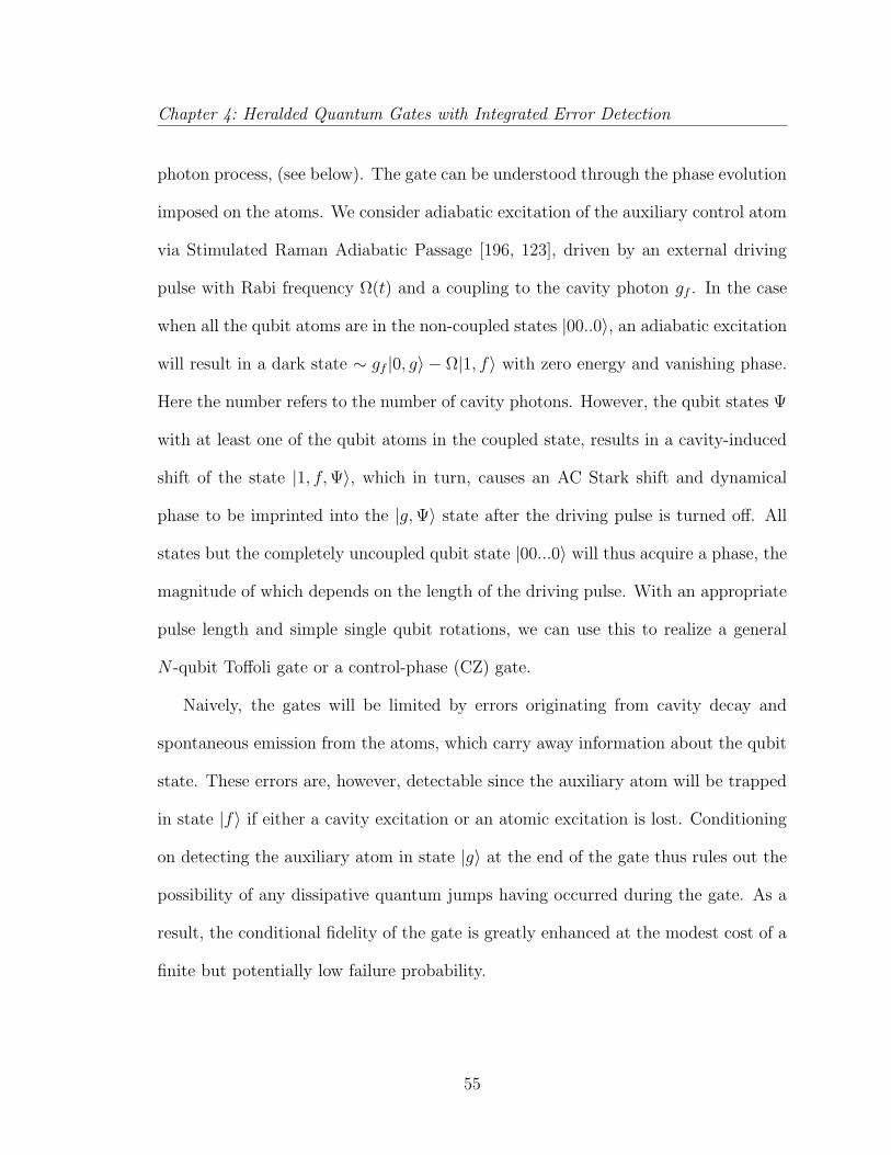
Chapter 4: Heralded Quantum Gates with Integrated Error Detection
photon process, (see below). The gate can be understood through the phase evolution
imposed on the atoms. We consider adiabatic excitation of the auxiliary control atom
via Stimulated Raman Adiabatic Passage [196, 123], driven by an external driving
pulse with Rabi frequency Ω(t) and a coupling to the cavity photon gf . In the case
when all the qubit atoms are in the non-coupled states |00..0〉, an adiabatic excitation
will result in a dark state ∼ gf |0, g〉 − Ω|1, f〉 with zero energy and vanishing phase.
Here the number refers to the number of cavity photons. However, the qubit states Ψ
with at least one of the qubit atoms in the coupled state, results in a cavity-induced
shift of the state |1, f,Ψ〉, which in turn, causes an AC Stark shift and dynamical
phase to be imprinted into the |g,Ψ〉 state after the driving pulse is turned off. All
states but the completely uncoupled qubit state |00...0〉 will thus acquire a phase, the
magnitude of which depends on the length of the driving pulse. With an appropriate
pulse length and simple single qubit rotations, we can use this to realize a general
N -qubit Toffoli gate or a control-phase (CZ) gate.
Naively, the gates will be limited by errors originating from cavity decay and
spontaneous emission from the atoms, which carry away information about the qubit
state. These errors are, however, detectable since the auxiliary atom will be trapped
in state |f〉 if either a cavity excitation or an atomic excitation is lost. Conditioning
on detecting the auxiliary atom in state |g〉 at the end of the gate thus rules out the
possibility of any dissipative quantum jumps having occurred during the gate. As a
result, the conditional fidelity of the gate is greatly enhanced at the modest cost of a
finite but potentially low failure probability.
55
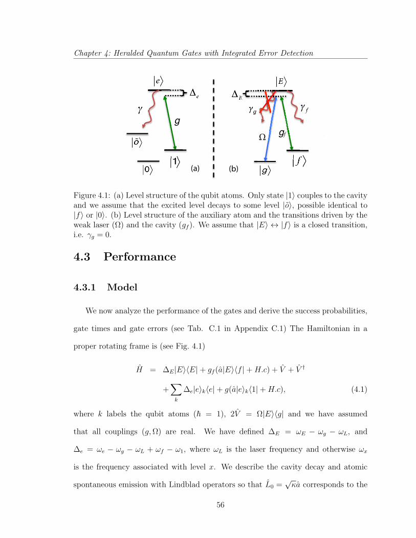
Chapter 4: Heralded Quantum Gates with Integrated Error Detection
!!
!
!
!
Ω gf
!
!
!! !
!
!
(b) (a)
g
!!
!
!
!
Ω gf
!
!
!! !
!
!
(b) (a)
g
Figure 4.1: (a) Level structure of the qubit atoms. Only state |1〉 couples to the cavityand we assume that the excited level decays to some level |o〉, possible identical to|f〉 or |0〉. (b) Level structure of the auxiliary atom and the transitions driven by theweak laser (Ω) and the cavity (gf ). We assume that |E〉 ↔ |f〉 is a closed transition,i.e. γg = 0.
4.3 Performance
4.3.1 Model
We now analyze the performance of the gates and derive the success probabilities,
gate times and gate errors (see Tab. C.1 in Appendix C.1) The Hamiltonian in a
proper rotating frame is (see Fig. 4.1)
H = ∆E|E〉〈E|+ gf (a|E〉〈f |+H.c) + V + V †
+∑
k
∆e|e〉k〈e|+ g(a|e〉k〈1|+H.c), (4.1)
where k labels the qubit atoms ( = 1), 2V = Ω|E〉〈g| and we have assumed
that all couplings (g,Ω) are real. We have defined ∆E = ωE − ωg − ωL, and
∆e = ωe − ωg − ωL + ωf − ω1, where ωL is the laser frequency and otherwise ωx
is the frequency associated with level x. We describe the cavity decay and atomic
spontaneous emission with Lindblad operators so that L0 =√κa corresponds to the
56
Chapter 4: Heralded Quantum Gates with Integrated Error Detection
cavity decay, Lf =√γf |f〉〈E| to the decay of the excited state of the auxiliary atom
and Lk =√γ|o〉k〈e| describes the decay of the excited qubit states to some arbitrary
ground state |o〉. The nature of |o〉 is not important for the dynamics of the gates
and it may or may not coincide with |0〉 or |1〉.
4.3.2 Effective Hamiltonian
We assume a weak driving pulse justifying for a perturbative treatment of V
using the formalism of Ref. [178]. In the perturbative description we adiabati-
cally eliminate the coupled excited states of the atoms and the cavity (assuming
Ω2/∆E ∆E and Ω g), which leads to an energy shift of the ground states but
otherwise conserves them since the Hamiltonian cannot connect different unexcited
states without decay. The dynamics are therefore described by an effective Hamilto-
nian, Heff = |g〉〈g|∑n ∆nPn where
∆n = Re
−Ω2
4γ((∆e
γ−i/2)i+2nC)
(2∆e
γ−i)((2∆E
γ−i)i/4+C)+(2∆E
γ−i)nC
(4.2)
and Pn projects on the states with n qubits in state |1〉. For simplicity, we have
assumed that the auxiliary atom is identical to the qubit atoms such that gf = g and
γf = γ (see Appendix C.1 for a more general treatment) and we have defined the
cooperativity C = g2/γκ. We consider the limit C 1 and from Eq. (4.2) we find
that the energy shift, in the case when all qubit atoms are in |0〉, becomes very small
∆0 ∼ ∆EΩ2/(16γ2C2)→ 0, i.e., we drive into a zero energy dark state as mentioned
in the description above. On the contrary, for n > 0, the C in the nominator of
∆n reflects that the coupling of the qubit atoms shifts the cavity resonance and as a
result an AC stark shift of ∼ Ω2/∆E is introduced. Furthermore, we find that in the
57
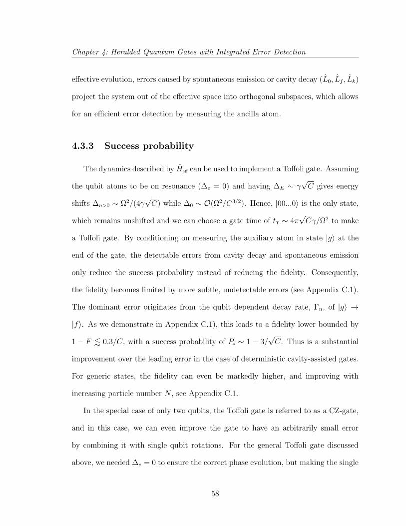
Chapter 4: Heralded Quantum Gates with Integrated Error Detection
effective evolution, errors caused by spontaneous emission or cavity decay (L0, Lf , Lk)
project the system out of the effective space into orthogonal subspaces, which allows
for an efficient error detection by measuring the ancilla atom.
4.3.3 Success probability
The dynamics described by Heff can be used to implement a Toffoli gate. Assuming
the qubit atoms to be on resonance (∆e = 0) and having ∆E ∼ γ√C gives energy
shifts ∆n>0 ∼ Ω2/(4γ√C) while ∆0 ∼ O(Ω2/C3/2). Hence, |00...0〉 is the only state,
which remains unshifted and we can choose a gate time of tT ∼ 4π√Cγ/Ω2 to make
a Toffoli gate. By conditioning on measuring the auxiliary atom in state |g〉 at the
end of the gate, the detectable errors from cavity decay and spontaneous emission
only reduce the success probability instead of reducing the fidelity. Consequently,
the fidelity becomes limited by more subtle, undetectable errors (see Appendix C.1).
The dominant error originates from the qubit dependent decay rate, Γn, of |g〉 →
|f〉. As we demonstrate in Appendix C.1), this leads to a fidelity lower bounded by
1 − F . 0.3/C, with a success probability of Ps ∼ 1 − 3/√C. Thus is a substantial
improvement over the leading error in the case of deterministic cavity-assisted gates.
For generic states, the fidelity can even be markedly higher, and improving with
increasing particle number N , see Appendix C.1.
In the special case of only two qubits, the Toffoli gate is referred to as a CZ-gate,
and in this case, we can even improve the gate to have an arbitrarily small error
by combining it with single qubit rotations. For the general Toffoli gate discussed
above, we needed ∆e = 0 to ensure the correct phase evolution, but making the single
58
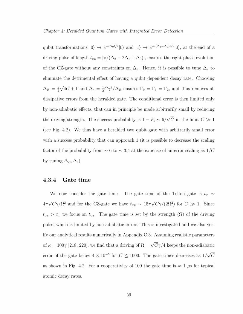
Chapter 4: Heralded Quantum Gates with Integrated Error Detection
qubit transformations |0〉 → e−i∆0t/2|0〉 and |1〉 → e−i(∆1−∆0)t/2|0〉, at the end of a
driving pulse of length tCZ = |π/(∆2 − 2∆1 + ∆0)|, ensures the right phase evolution
of the CZ-gate without any constraints on ∆e. Hence, it is possible to tune ∆e to
eliminate the detrimental effect of having a qubit dependent decay rate. Choosing
∆E = γ2
√4C + 1 and ∆e = 1
2Cγ2/∆E ensures Γ0 = Γ1 = Γ2, and thus removes all
dissipative errors from the heralded gate. The conditional error is then limited only
by non-adiabatic effects, that can in principle be made arbitrarily small by reducing
the driving strength. The success probability is 1 − Ps ∼ 6/√C in the limit C 1
(see Fig. 4.2). We thus have a heralded two qubit gate with arbitrarily small error
with a success probability that can approach 1 (it is possible to decrease the scaling
factor of the probability from ∼ 6 to ∼ 3.4 at the expense of an error scaling as 1/C
by tuning ∆E,∆e).
4.3.4 Gate time
We now consider the gate time. The gate time of the Toffoli gate is tT ∼
4π√Cγ/Ω2 and for the CZ-gate we have tCZ ∼ 15π
√Cγ/(2Ω2) for C 1. Since
tCZ > tT we focus on tCZ. The gate time is set by the strength (Ω) of the driving
pulse, which is limited by non-adiabatic errors. This is investigated and we also ver-
ify our analytical results numerically in Appendix C.3. Assuming realistic parameters
of κ = 100γ [218, 220], we find that a driving of Ω =√Cγ/4 keeps the non-adiabatic
error of the gate below 4 × 10⁻⁵ for C ≤ 1000. The gate times decreases as 1/√C
as shown in Fig. 4.2. For a cooperativity of 100 the gate time is ≈ 1 µs for typical
atomic decay rates.
59
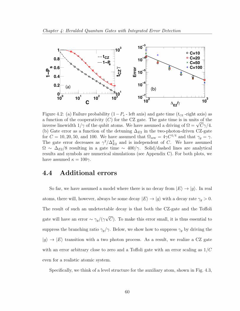
Chapter 4: Heralded Quantum Gates with Integrated Error Detection
100 101 102 1030
0.2
0.4
0.6
0.8
1
C
1−P s
101
102
103
t CZγ
data1 tCZ
data31−Ps
data5data6 (a)
1001000 10−7
10−6
10−5
10−4
10−3
ΔE2/γ
Error
data1
C=10C=20C=50C=100
10 1032
(b)
Figure 4.2: (a) Failure probability (1−Ps - left axis) and gate time (tCZ -right axis) asa function of the cooperativity (C) for the CZ gate. The gate time is in units of theinverse linewidth 1/γ of the qubit atoms. We have assumed a driving of Ω =
√Cγ/4.
(b) Gate error as a function of the detuning ∆E2 in the two-photon-driven CZ-gatefor C = 10, 20, 50, and 100. We have assumed that ΩMW = 4γC1/4 and that γg = γ.The gate error decreases as γ2/∆2
E2 and is independent of C. We have assumedΩ ∼ ∆E2/8 resulting in a gate time ∼ 400/γ. Solid/dashed lines are analyticalresults and symbols are numerical simulations (see Appendix C). For both plots, wehave assumed κ = 100γ.
4.4 Additional errors
So far, we have assumed a model where there is no decay from |E〉 → |g〉. In real
atoms, there will, however, always be some decay |E〉 → |g〉 with a decay rate γg > 0.
The result of such an undetectable decay is that both the CZ-gate and the Toffoli
gate will have an error ∼ γg/(γ√C). To make this error small, it is thus essential to
suppress the branching ratio γg/γ. Below, we show how to suppress γg by driving the
|g〉 → |E〉 transition with a two photon process. As a result, we realize a CZ gate
with an error arbitrary close to zero and a Toffoli gate with an error scaling as 1/C
even for a realistic atomic system.
Specifically, we think of a level structure for the auxiliary atom, shown in Fig. 4.3,
60
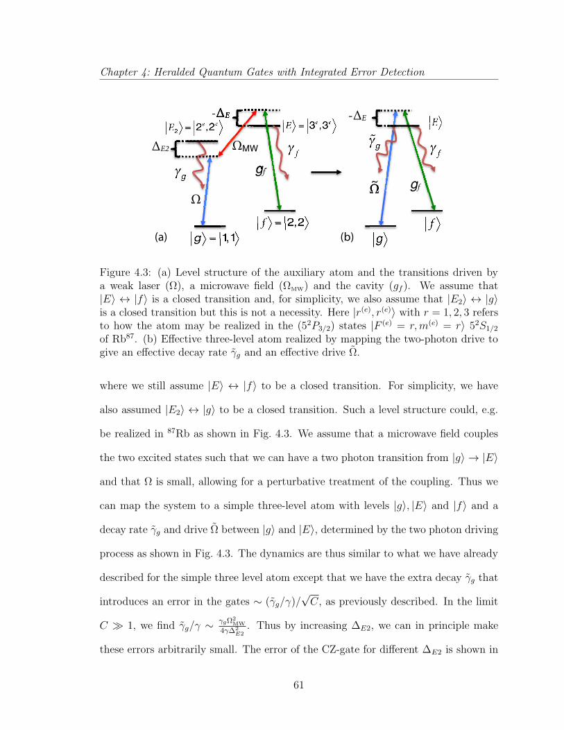
Chapter 4: Heralded Quantum Gates with Integrated Error Detection
!!!!!!!!
!
!
!
!
Ω
gf!
-ΔE
gfgfg
-ΔE
ΩMW
!
!!!!!!ΔE2 !
!
!
!
!
gf!
-ΔE
Ω ΩΩΩΩ~
!
!
!
!
(a) (b)
Figure 4.3: (a) Level structure of the auxiliary atom and the transitions driven bya weak laser (Ω), a microwave field (ΩMW) and the cavity (gf ). We assume that|E〉 ↔ |f〉 is a closed transition and, for simplicity, we also assume that |E2〉 ↔ |g〉is a closed transition but this is not a necessity. Here |r(e), r(e)〉 with r = 1, 2, 3 refersto how the atom may be realized in the (52P3/2) states |F (e) = r,m(e) = r〉 52S1/2
of Rb87. (b) Effective three-level atom realized by mapping the two-photon drive togive an effective decay rate γg and an effective drive Ω.
where we still assume |E〉 ↔ |f〉 to be a closed transition. For simplicity, we have
also assumed |E2〉 ↔ |g〉 to be a closed transition. Such a level structure could, e.g.
be realized in 87Rb as shown in Fig. 4.3. We assume that a microwave field couples
the two excited states such that we can have a two photon transition from |g〉 → |E〉
and that Ω is small, allowing for a perturbative treatment of the coupling. Thus we
can map the system to a simple three-level atom with levels |g〉, |E〉 and |f〉 and a
decay rate γg and drive Ω between |g〉 and |E〉, determined by the two photon driving
process as shown in Fig. 4.3. The dynamics are thus similar to what we have already
described for the simple three level atom except that we have the extra decay γg that
introduces an error in the gates ∼ (γg/γ)/√C, as previously described. In the limit
C 1, we find γg/γ ∼ γgΩ2MW
4γ∆2E2
. Thus by increasing ∆E2, we can in principle make
these errors arbitrarily small. The error of the CZ-gate for different ∆E2 is shown in
61
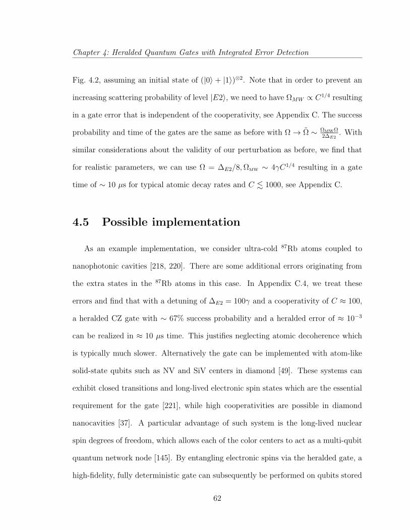
Chapter 4: Heralded Quantum Gates with Integrated Error Detection
Fig. 4.2, assuming an initial state of (|0〉 + |1〉)⊗2. Note that in order to prevent an
increasing scattering probability of level |E2〉, we need to have ΩMW ∝ C1/4 resulting
in a gate error that is independent of the cooperativity, see Appendix C. The success
probability and time of the gates are the same as before with Ω→ Ω ∼ ΩMWΩ2∆E2
. With
similar considerations about the validity of our perturbation as before, we find that
for realistic parameters, we can use Ω = ∆E2/8,ΩMW ∼ 4γC1/4 resulting in a gate
time of ∼ 10 µs for typical atomic decay rates and C . 1000, see Appendix C.
4.5 Possible implementation
As an example implementation, we consider ultra-cold 87Rb atoms coupled to
nanophotonic cavities [218, 220]. There are some additional errors originating from
the extra states in the 87Rb atoms in this case. In Appendix C.4, we treat these
errors and find that with a detuning of ∆E2 = 100γ and a cooperativity of C ≈ 100,
a heralded CZ gate with ∼ 67% success probability and a heralded error of ≈ 10−3
can be realized in ≈ 10 µs time. This justifies neglecting atomic decoherence which
is typically much slower. Alternatively the gate can be implemented with atom-like
solid-state qubits such as NV and SiV centers in diamond [49]. These systems can
exhibit closed transitions and long-lived electronic spin states which are the essential
requirement for the gate [221], while high cooperativities are possible in diamond
nanocavities [37]. A particular advantage of such system is the long-lived nuclear
spin degrees of freedom, which allows each of the color centers to act as a multi-qubit
quantum network node [145]. By entangling electronic spins via the heralded gate, a
high-fidelity, fully deterministic gate can subsequently be performed on qubits stored
62
Chapter 4: Heralded Quantum Gates with Integrated Error Detection
in nuclear spins [208].
4.6 Application
As a particular application, we consider a quantum repeater where entanglement
is first created in small segments (links), which are subsequently connected using
entanglement swapping [33]. By organizing the repeater in a tree structure, the
probabilistic nature of the gate can be efficiently circumvented. The success rate of
distributing entanglement across the total distance L, scales as ∼ (L/L0)1−log2(3/p),
where p < 1 is the success probability of the swap, L is the total distribution distance
and L0 is the length between the links [25] (note that in the limit p → 1, the above
expression underestimates the rate, e.g., for p = 1 the actual rate is ∼ 3 times faster
for 128 links). This is a substantial improvement over direct transmission where the
success rate scales exponentially with L. For a realization with nuclear spin memories
where the swap can be performed deterministically the rate can scale even better as
∼ log2(L/L0)−1. In order to maintain the favorable scaling without resorting to
time consuming purification, the total number of links, Nmax should be kept below
Nmax ∼ − ln(Ffinal)/(ε0 + εg), where Ffinal is the required fidelity of the final distributed
pair and ε0, εg 1 are the errors of the initial entanglement generation and the
entanglement swapping respectively. Thus, it is essential that the errors are kept
small, which can be obtained with the heralded gate.
63
Chapter 4: Heralded Quantum Gates with Integrated Error Detection
4.7 Conclusion
In conclusion, we have introduced a heralded two-qubit quantum gate with a con-
ditional fidelity arbitrarily close to unity and an N -qubit Toffoli gate with an error
scaling as 1/C. The gates have a built-in error detection process, which removes the
necessity of extracting the error by the more complicated process of entanglement
purification or quantum error correction. Our gate is designed for the specific case of
optical cavities, and allows exploiting realistic systems for quantum communication,
even though the error rate would inhibit this with deterministic gates. Similar ad-
vantages can be realized in other systems such as those based on circuit QED, where
certain errors could be heralded and thus alleviate the daunting requirements of fault
tolerant computation.
64
Chapter 5
Remote entanglement distribution
using individual atoms in cavities
5.1 Introduction
Distribution of entanglement is an essential task in quantum communication [117,
54, 169]. Entanglement can be used to make highly secure communication channels
due to the sensitivity of entangled quantum systems to external influences [195].
While this sensitivity makes it possible to detect any attack from an eavesdropper,
it also makes it hard to distribute entanglement over large distances since any noise
from the environment quickly destroys the entanglement. Direct transmission of a
quantum signal suffers from loss and decoherence from the transmission channel,
which results in an exponential decrease of the rate with distance [33]. To overcome
this problem, it has been proposed to use quantum repeaters, where entanglement is
first created over short distances by direct transmission and then stored in quantum
65
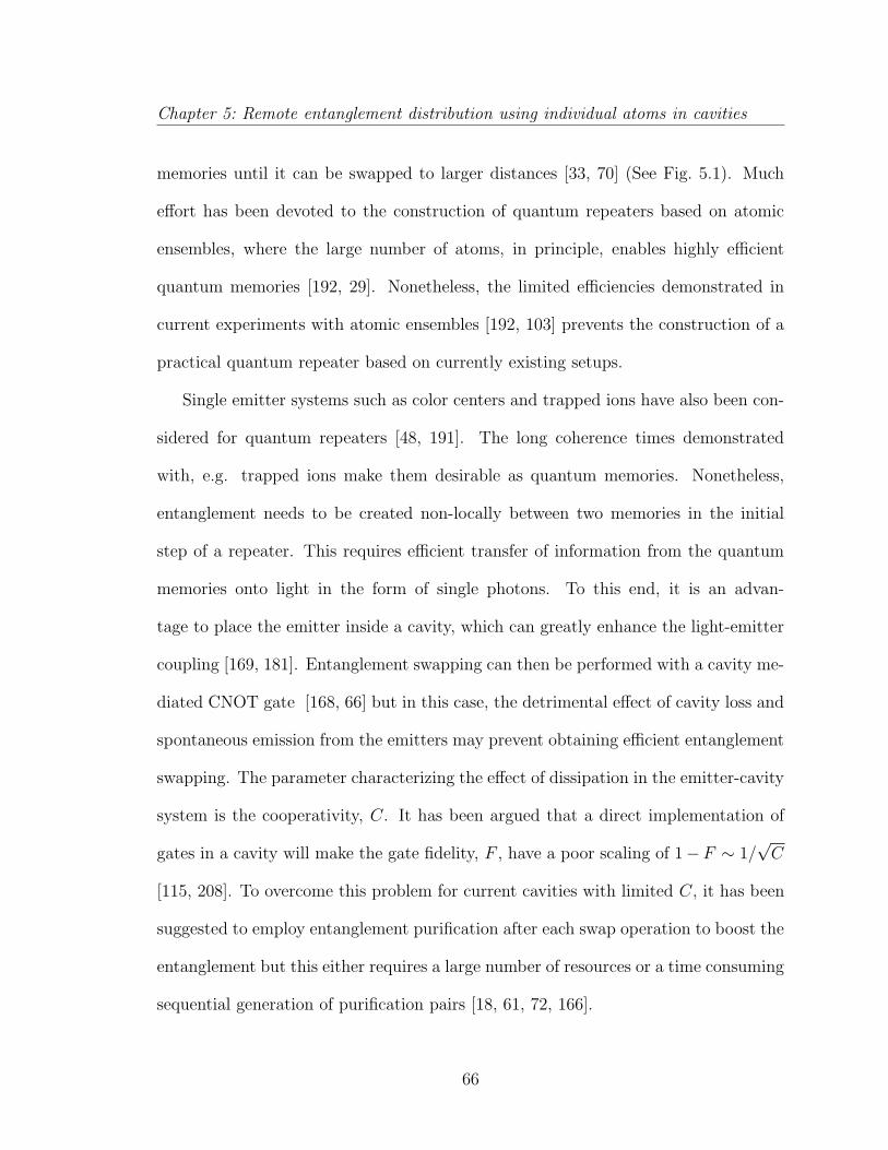
Chapter 5: Remote entanglement distribution using individual atoms in cavities
memories until it can be swapped to larger distances [33, 70] (See Fig. 5.1). Much
effort has been devoted to the construction of quantum repeaters based on atomic
ensembles, where the large number of atoms, in principle, enables highly efficient
quantum memories [192, 29]. Nonetheless, the limited efficiencies demonstrated in
current experiments with atomic ensembles [192, 103] prevents the construction of a
practical quantum repeater based on currently existing setups.
Single emitter systems such as color centers and trapped ions have also been con-
sidered for quantum repeaters [48, 191]. The long coherence times demonstrated
with, e.g. trapped ions make them desirable as quantum memories. Nonetheless,
entanglement needs to be created non-locally between two memories in the initial
step of a repeater. This requires efficient transfer of information from the quantum
memories onto light in the form of single photons. To this end, it is an advan-
tage to place the emitter inside a cavity, which can greatly enhance the light-emitter
coupling [169, 181]. Entanglement swapping can then be performed with a cavity me-
diated CNOT gate [168, 66] but in this case, the detrimental effect of cavity loss and
spontaneous emission from the emitters may prevent obtaining efficient entanglement
swapping. The parameter characterizing the effect of dissipation in the emitter-cavity
system is the cooperativity, C. It has been argued that a direct implementation of
gates in a cavity will make the gate fidelity, F , have a poor scaling of 1−F ∼ 1/√C
[115, 208]. To overcome this problem for current cavities with limited C, it has been
suggested to employ entanglement purification after each swap operation to boost the
entanglement but this either requires a large number of resources or a time consuming
sequential generation of purification pairs [18, 61, 72, 166].
66

Chapter 5: Remote entanglement distribution using individual atoms in cavities
Here we analyze and compare a number of cavity-based quantum repeaters which
combines various proposals for entanglement generation and cavity-assisted CNOT
gates. We find that the best scheme is where high-fidelity entanglement is gener-
ated using a two-photon detection scheme similar to Ref. [68] and swapped to large
distances using the heralded CZ-gate proposed in Ref. [26]. The heralded gate en-
ables nearly perfect entanglement swapping when successful allowing for many swaps
without the need of entanglement purification. As a result, high-rate entanglement
distribution is achieved even for low cooperativities.
Compared to the other cavity-based repeaters, this high-fidelity repeater achieves
up to two orders of magnitude higher secret key rate (see below) for realistic pa-
rameters and large distances (1000 km). Specifically, we have compared to repeaters
where entanglement is generated using a single-photon detection scheme similar to
Ref. [35], which allows for a better rate at the expense of fidelity. Furthermore, we
have considered schemes where entanglement swapping is achieved using the deter-
ministic CNOT gate suggested in Ref. [208], combining it with the local entanglement
generation scheme of Ref. [209]. The advantage of this gate is that the fidelity scales
as 1− F ∼ 1/C, which is a significant improvement from the 1/√C scaling, charac-
terizing the performance of a direct implementation of gates in a cavity. As a result,
long-distance entanglement distribution can also be achieved with this gate but it
requires cooperativities above 100, which might be challenging to achieve experimen-
tally. Furthermore, we include the possibility of initial purification in repeaters based
on the single-photon detection scheme in order to allow for the higher rate of this
scheme to compensate for the lower fidelity compared to the two-photon detection
67
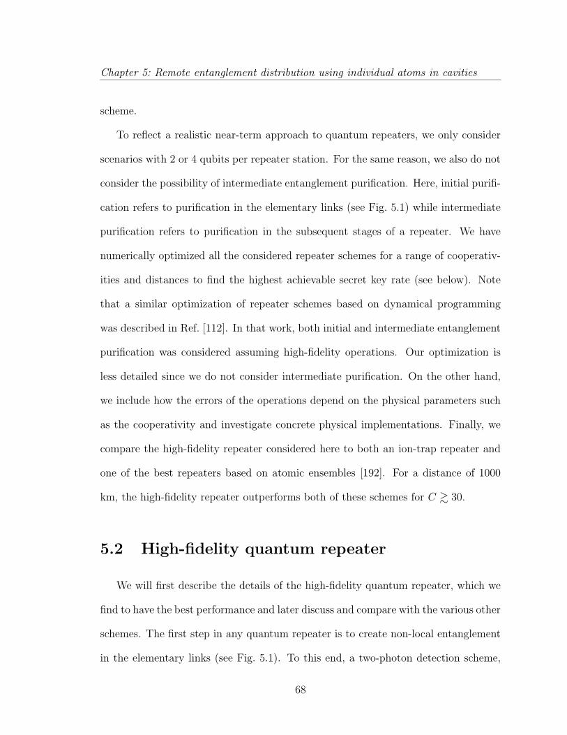
Chapter 5: Remote entanglement distribution using individual atoms in cavities
scheme.
To reflect a realistic near-term approach to quantum repeaters, we only consider
scenarios with 2 or 4 qubits per repeater station. For the same reason, we also do not
consider the possibility of intermediate entanglement purification. Here, initial purifi-
cation refers to purification in the elementary links (see Fig. 5.1) while intermediate
purification refers to purification in the subsequent stages of a repeater. We have
numerically optimized all the considered repeater schemes for a range of cooperativ-
ities and distances to find the highest achievable secret key rate (see below). Note
that a similar optimization of repeater schemes based on dynamical programming
was described in Ref. [112]. In that work, both initial and intermediate entanglement
purification was considered assuming high-fidelity operations. Our optimization is
less detailed since we do not consider intermediate purification. On the other hand,
we include how the errors of the operations depend on the physical parameters such
as the cooperativity and investigate concrete physical implementations. Finally, we
compare the high-fidelity repeater considered here to both an ion-trap repeater and
one of the best repeaters based on atomic ensembles [192]. For a distance of 1000
km, the high-fidelity repeater outperforms both of these schemes for C & 30.
5.2 High-fidelity quantum repeater
We will first describe the details of the high-fidelity quantum repeater, which we
find to have the best performance and later discuss and compare with the various other
schemes. The first step in any quantum repeater is to create non-local entanglement
in the elementary links (see Fig. 5.1). To this end, a two-photon detection scheme,
68
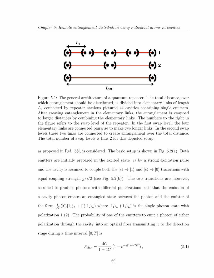
Chapter 5: Remote entanglement distribution using individual atoms in cavities
Figure 5.1: The general architecture of a quantum repeater. The total distance, overwhich entanglement should be distributed, is divided into elementary links of lengthL0 connected by repeater stations pictured as cavities containing single emitters.After creating entanglement in the elementary links, the entanglement is swappedto larger distances by combining the elementary links. The numbers to the right inthe figure refers to the swap level of the repeater. In the first swap level, the fourelementary links are connected pairwise to make two longer links. In the second swaplevels these two links are connected to create entanglement over the total distance.The total number of swap levels is thus 2 for this depicted setup.
as proposed in Ref. [68], is considered. The basic setup is shown in Fig. 5.2(a). Both
emitters are initially prepared in the excited state |e〉 by a strong excitation pulse
and the cavity is assumed to couple both the |e〉 → |1〉 and |e〉 → |0〉 transitions with
equal coupling strength g/√2 (see Fig. 5.2(b)). The two transitions are, however,
assumed to produce photons with different polarizations such that the emission of
a cavity photon creates an entangled state between the photon and the emitter of
the form 1√2(|0〉|11〉L + |1〉|12〉L) where |11〉L (|12〉L) is the single photon state with
polarization 1 (2). The probability of one of the emitters to emit a photon of either
polarization through the cavity, into an optical fiber transmitting it to the detection
stage during a time interval [0; T ] is
Pphot =4C
1 + 4C
(1− e−γ(1+4C)T
), (5.1)
69
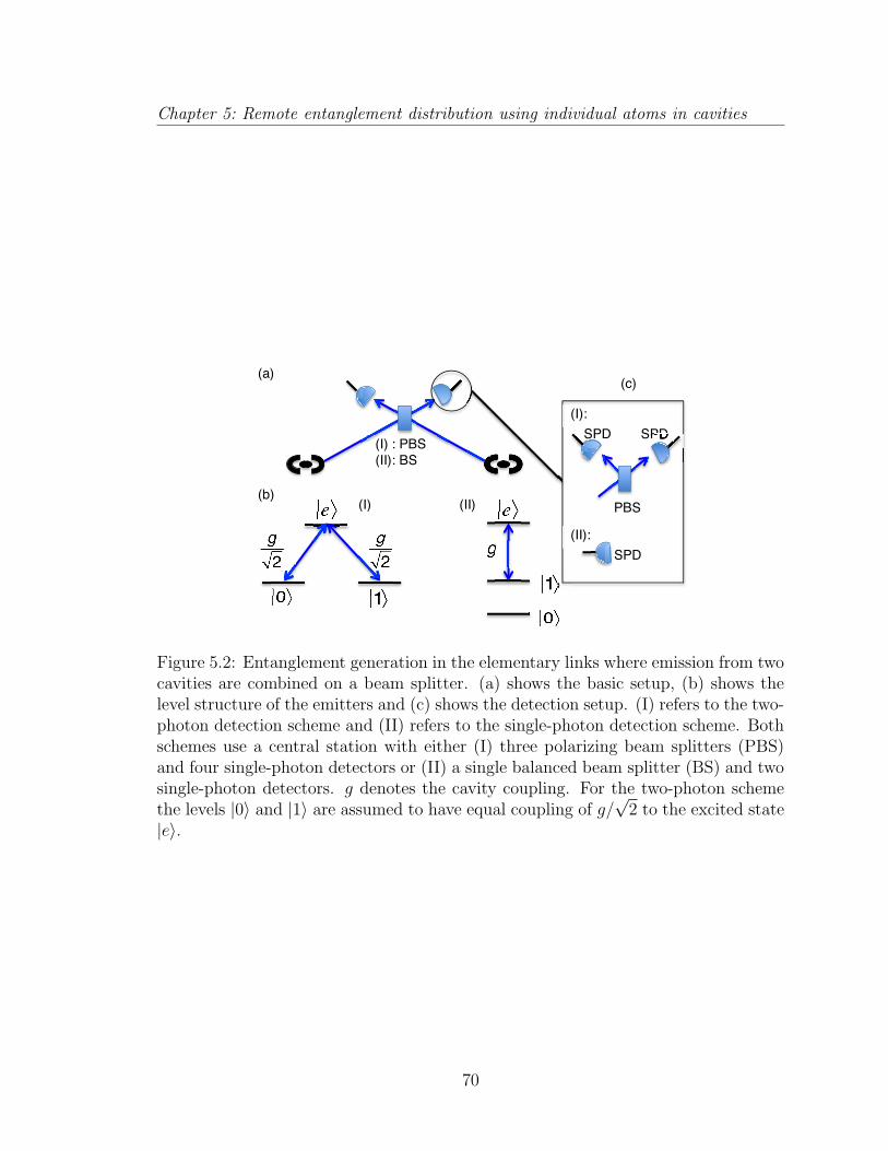
Chapter 5: Remote entanglement distribution using individual atoms in cavities
!
!
!
!
!
(I)
!!
!
!!
(II)
(I) : PBS (II): BS
(I):
(II): SPD
SPD SPD
PBS
SPD
(a)
(b)
(c)
Figure 5.2: Entanglement generation in the elementary links where emission from twocavities are combined on a beam splitter. (a) shows the basic setup, (b) shows thelevel structure of the emitters and (c) shows the detection setup. (I) refers to the two-photon detection scheme and (II) refers to the single-photon detection scheme. Bothschemes use a central station with either (I) three polarizing beam splitters (PBS)and four single-photon detectors or (II) a single balanced beam splitter (BS) and twosingle-photon detectors. g denotes the cavity coupling. For the two-photon schemethe levels |0〉 and |1〉 are assumed to have equal coupling of g/
√2 to the excited state
|e〉.
70
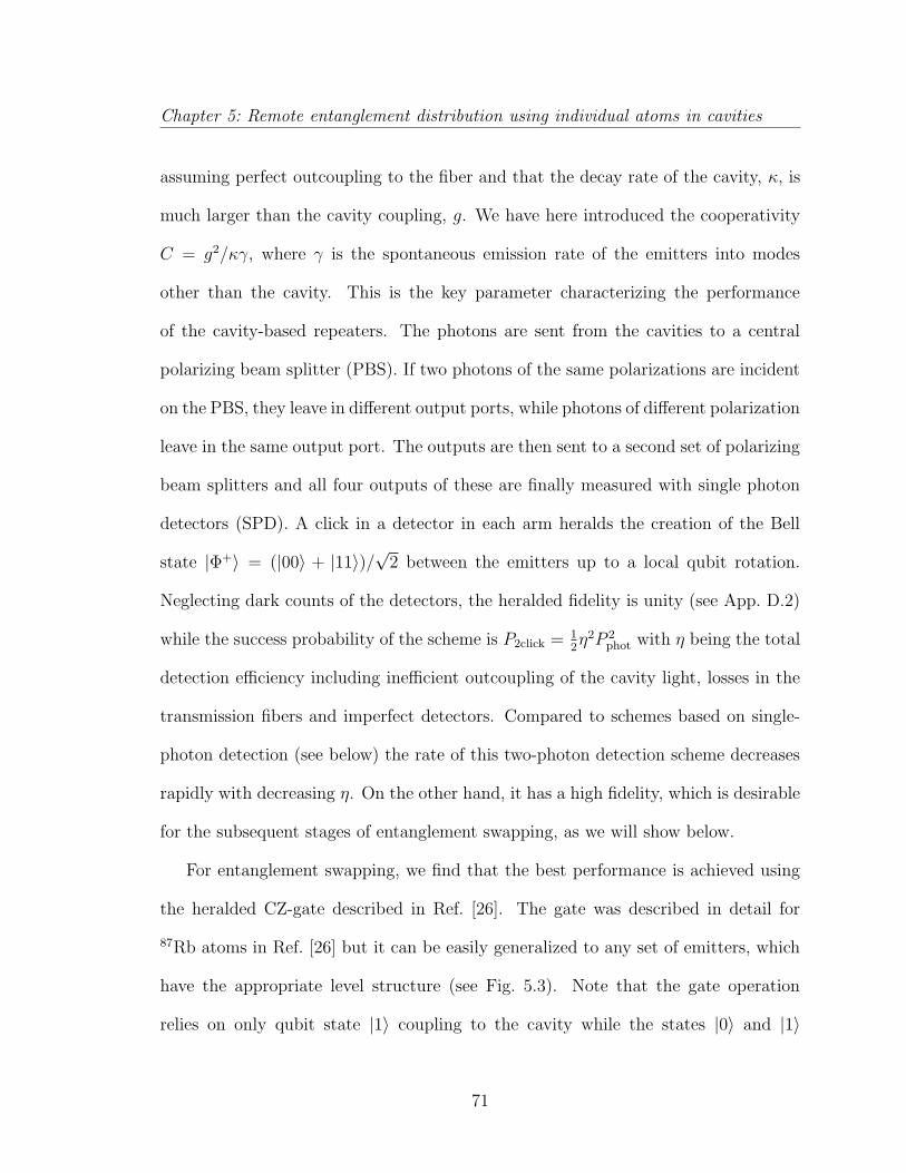
Chapter 5: Remote entanglement distribution using individual atoms in cavities
assuming perfect outcoupling to the fiber and that the decay rate of the cavity, κ, is
much larger than the cavity coupling, g. We have here introduced the cooperativity
C = g2/κγ, where γ is the spontaneous emission rate of the emitters into modes
other than the cavity. This is the key parameter characterizing the performance
of the cavity-based repeaters. The photons are sent from the cavities to a central
polarizing beam splitter (PBS). If two photons of the same polarizations are incident
on the PBS, they leave in different output ports, while photons of different polarization
leave in the same output port. The outputs are then sent to a second set of polarizing
beam splitters and all four outputs of these are finally measured with single photon
detectors (SPD). A click in a detector in each arm heralds the creation of the Bell
state |Φ+〉 = (|00〉 + |11〉)/√
2 between the emitters up to a local qubit rotation.
Neglecting dark counts of the detectors, the heralded fidelity is unity (see App. D.2)
while the success probability of the scheme is P2click = 12η2P 2
phot with η being the total
detection efficiency including inefficient outcoupling of the cavity light, losses in the
transmission fibers and imperfect detectors. Compared to schemes based on single-
photon detection (see below) the rate of this two-photon detection scheme decreases
rapidly with decreasing η. On the other hand, it has a high fidelity, which is desirable
for the subsequent stages of entanglement swapping, as we will show below.
For entanglement swapping, we find that the best performance is achieved using
the heralded CZ-gate described in Ref. [26]. The gate was described in detail for
87Rb atoms in Ref. [26] but it can be easily generalized to any set of emitters, which
have the appropriate level structure (see Fig. 5.3). Note that the gate operation
relies on only qubit state |1〉 coupling to the cavity while the states |0〉 and |1〉
71
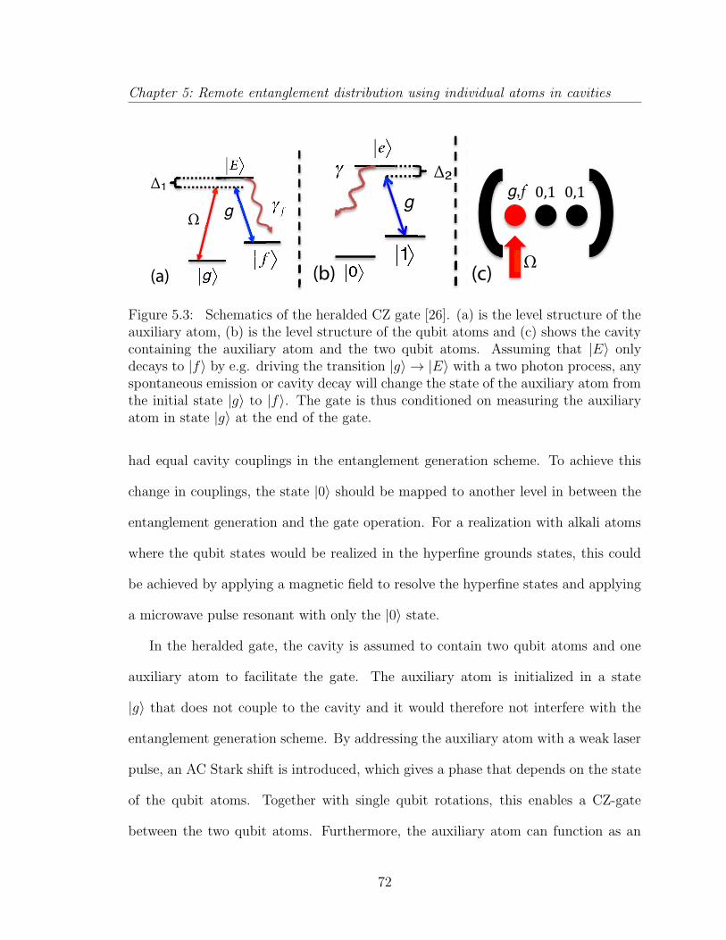
Chapter 5: Remote entanglement distribution using individual atoms in cavities
!!
!
!
!
Ω g
Δ1
!
!
g
Δ2 !
!
!
! Ω (a) (b) (c)
g,f 0,1! 0,1!
!!
!
!
!
Ω g
Δ1
!
!
g
Δ2 !
!
!
!
2
Ω (a) (b) (c)
g,f 0,1! 0,1!
!!
!
!
!
Ω g
Δ1
!
!
g
Δ2 !
!
!
! Ω (a) (b) (c)
g,f f 0,1! 0,1!
Figure 5.3: Schematics of the heralded CZ gate [26]. (a) is the level structure of theauxiliary atom, (b) is the level structure of the qubit atoms and (c) shows the cavitycontaining the auxiliary atom and the two qubit atoms. Assuming that |E〉 onlydecays to |f〉 by e.g. driving the transition |g〉 → |E〉 with a two photon process, anyspontaneous emission or cavity decay will change the state of the auxiliary atom fromthe initial state |g〉 to |f〉. The gate is thus conditioned on measuring the auxiliaryatom in state |g〉 at the end of the gate.
had equal cavity couplings in the entanglement generation scheme. To achieve this
change in couplings, the state |0〉 should be mapped to another level in between the
entanglement generation and the gate operation. For a realization with alkali atoms
where the qubit states would be realized in the hyperfine grounds states, this could
be achieved by applying a magnetic field to resolve the hyperfine states and applying
a microwave pulse resonant with only the |0〉 state.
In the heralded gate, the cavity is assumed to contain two qubit atoms and one
auxiliary atom to facilitate the gate. The auxiliary atom is initialized in a state
|g〉 that does not couple to the cavity and it would therefore not interfere with the
entanglement generation scheme. By addressing the auxiliary atom with a weak laser
pulse, an AC Stark shift is introduced, which gives a phase that depends on the state
of the qubit atoms. Together with single qubit rotations, this enables a CZ-gate
between the two qubit atoms. Furthermore, the auxiliary atom can function as an
72
Chapter 5: Remote entanglement distribution using individual atoms in cavities
error detector in the sense that any cavity decay or spontaneous emission changes the
state of the atom. Performing a heralding measurement of the state of the auxiliary
atom at the end of the driving pulse removes all dissipative errors. As a consequence,
the gate gets limited only by non-adiabatic effects. As shown in Ref. [26], a heralded
error below 4 × 10⁻⁵ is possible with a gate time of ∼ 377/(γ√C), where γ is the
atomic linewidth. The failure probability of the gate scales as 1/√C and the high
fidelity thus comes at the cost of a finite but possibly low failure probability. A CZ
gate combined with single qubit rotations is sufficient to perform direct entanglement
swapping. For simplicity, we assume perfect single qubit rotations and 100% efficient
measurement of atomic states for all schemes considered. Relaxing this assumption
will in general decrease the rate of all the considered repeater schemes but schemes
with a high number of swap levels, such as the high-fidelity repeater, will be influenced
more on the rate than schemes with a low number of swap levels.
The advantage of the high-fidelity repeater can be understood by considering the
requirement for reaching a certain threshold fidelity, Ffinal of the distributed pair. In
this case, the maximum number of swap levels is Nmax ∼ − log2(Ffinal/(ε0+εg)), where
ε0, εg 1 are the errors of the initial entanglement generation and the entanglement
swapping respectively. The combination of the high-fidelity two-photon detection
scheme and the heralded gate thus makes it possible to have a repeater with many
elementary links while maintaining a high fidelity of the final distributed pair even
for low cooperativities since the error of the heralded gate is still high in this regime.
73
Chapter 5: Remote entanglement distribution using individual atoms in cavities
5.2.1 Secret key rate
We imagine that the distributed entanglement is used to generate a secret key
between two parties referred to as Alice and Bob. There exist various quantum key
distribution schemes [195, 17, 80, 36], however, the general idea is that Alice and Bob
can exclude that an eavesdropper has any information about the key by measuring
their qubits and comparing results. We will assume that a six-state version of the
BB84 protocol described in Ref. [36] is used to generate the secret key. This protocol
consists of three main steps. First Alice and Bob picks a basis according to some prob-
ability distribution and measure the state of their qubits thereby producing two bit
strings referred to as the raw key. Afterwards they compare their choice of basis and
only keep the bits where they chose the same measurement basis thereby producing
a sifted key. Finally, Alice and Bob estimate the information that some eavesdropper
could possibly have obtained about their key and perform privacy amplification [195].
If the errors are not too big, they can obtain a shorter but completely secure key. For
the six-state protocol, the secret key rate, rsecret can be defined as
rsecret = rdistpsiftfsecret, (5.2)
where rdist is the distribution rate of the entangled pairs, psift is the probability that
Alice and Bob choose the same measurement basis and fsecret is the secret key fraction,
which depends on the fidelity of the distributed pairs. We assume a worst case scenario
where the distributed pairs are Werner states of the form
ρ = F |Φ+〉〈Φ+|+ 1− F3
(|Φ−〉〈Φ−|+ |Ψ+〉〈Ψ+|+ |Ψ−〉〈Ψ−|
). (5.3)
74
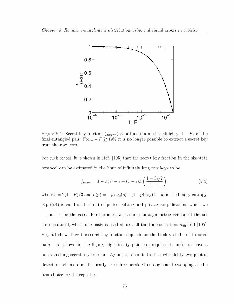
Chapter 5: Remote entanglement distribution using individual atoms in cavities
10−4
10−3
10−2
10−1
0
0.2
0.4
0.6
0.8
1
1−F
f secre
t
Figure 5.4: Secret key fraction (fsecret) as a function of the infidelity, 1 − F , of thefinal entangled pair. For 1− F & 19% it is no longer possible to extract a secret keyfrom the raw keys.
For such states, it is shown in Ref. [195] that the secret key fraction in the six-state
protocol can be estimated in the limit of infinitely long raw keys to be
fsecret = 1− h(ε)− ε+ (1− ε)h(
1− 3ε/2
1− ε
), (5.4)
where ε = 2(1−F )/3 and h(p) = −plog2(p)− (1−p)log2(1−p) is the binary entropy.
Eq. (5.4) is valid in the limit of perfect sifting and privacy amplification, which we
assume to be the case. Furthermore, we assume an asymmetric version of the six
state protocol, where one basis is used almost all the time such that psift ≈ 1 [195].
Fig. 5.4 shows how the secret key fraction depends on the fidelity of the distributed
pairs. As shown in the figure, high-fidelity pairs are required in order to have a
non-vanishing secret key fraction. Again, this points to the high-fidelity two-photon
detection scheme and the nearly error-free heralded entanglement swapping as the
best choice for the repeater.
75
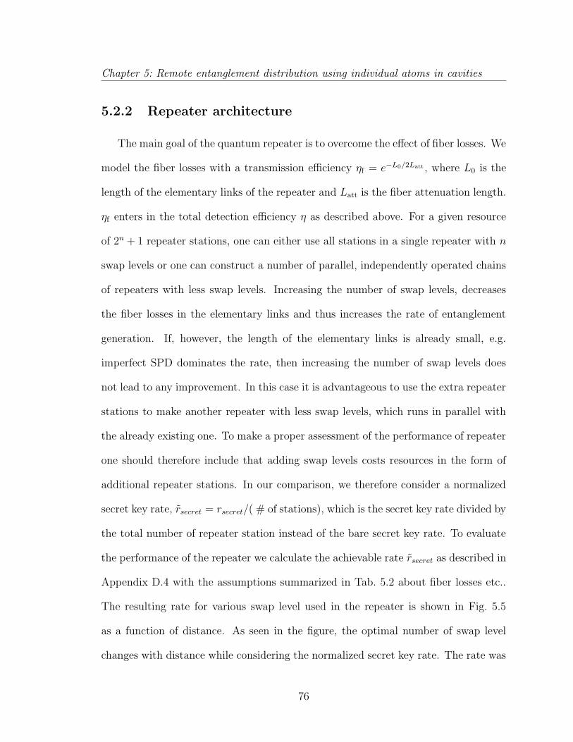
Chapter 5: Remote entanglement distribution using individual atoms in cavities
5.2.2 Repeater architecture
The main goal of the quantum repeater is to overcome the effect of fiber losses. We
model the fiber losses with a transmission efficiency ηf = e−L0/2Latt , where L0 is the
length of the elementary links of the repeater and Latt is the fiber attenuation length.
ηf enters in the total detection efficiency η as described above. For a given resource
of 2n + 1 repeater stations, one can either use all stations in a single repeater with n
swap levels or one can construct a number of parallel, independently operated chains
of repeaters with less swap levels. Increasing the number of swap levels, decreases
the fiber losses in the elementary links and thus increases the rate of entanglement
generation. If, however, the length of the elementary links is already small, e.g.
imperfect SPD dominates the rate, then increasing the number of swap levels does
not lead to any improvement. In this case it is advantageous to use the extra repeater
stations to make another repeater with less swap levels, which runs in parallel with
the already existing one. To make a proper assessment of the performance of repeater
one should therefore include that adding swap levels costs resources in the form of
additional repeater stations. In our comparison, we therefore consider a normalized
secret key rate, rsecret = rsecret/( # of stations), which is the secret key rate divided by
the total number of repeater station instead of the bare secret key rate. To evaluate
the performance of the repeater we calculate the achievable rate rsecret as described in
Appendix D.4 with the assumptions summarized in Tab. 5.2 about fiber losses etc..
The resulting rate for various swap level used in the repeater is shown in Fig. 5.5
as a function of distance. As seen in the figure, the optimal number of swap level
changes with distance while considering the normalized secret key rate. The rate was
76
Chapter 5: Remote entanglement distribution using individual atoms in cavities
100 200 300 400 50010−1
100
101
Distance [km]
r secr
et [H
z]
n=1n=2n=3
~
Figure 5.5: Normalized secret key rate per station(rsecret) as a function of the distri-bution distance for a high-fidelity repeater consisting of the two-photon entanglementgeneration scheme and the heralded gate for entanglement swapping. We have con-sidered n = 2, 3 and 4 swap levels and have assumed a cooperativity of C =100 andtwo qubits per repeater station. The secret key rate was calculated as described inApp. D.4 with the assumptions summarized in Tab. 5.2.
calculated as described in App. D.4 for a cooperativity of 100 with the assumptions
summarized in Tab. 5.2 about fiber losses, detection efficiencies etc. For distances
. 150 km, only a single swap level is needed since the fiber losses are relatively small
while more swap levels are needed as the distance increases.
In most repeater schemes, the qubits in each repeater station are assumed to be
operated simultaneously with half of the qubits being used to generate entanglement
with the neighboring station to each side such that entanglement attempts in all the
elementary links are done simultaneously. We will refer to this as a parallel repeater.
We will, however, also consider another sequential way of operating the qubits, where
all qubits in a station are first used to make entanglement in one elementary link.
77
Chapter 5: Remote entanglement distribution using individual atoms in cavities
After this has been obtained, all but one qubit are then used to make entanglement
over the neighboring link in the opposite direction. This is referred to as a sequential
repeater. The advantage of the sequential repeater is that the rate of the lowest level
in the repeater, the entanglement generation, is increased. This comes at the cost of a
waiting time between entanglement attempts in neighboring links. As the number of
qubits per repeater station increases the sequential repeater will start to outperform
the parallel repeater. We find that this happens with 4 qubits per repeater station
(see Sec. 5.4).
5.3 Other cavity based repeaters
We have found that the high-fidelity repeater that we have described above out-
performs a number of other cavity-based repeater schemes, which can be constructed
with different schemes of entanglement generation and CNOT gates. Below, we de-
scribe the constituents of these other schemes and compare them to those of the
high-fidelity repeater
5.3.1 Single-photon entanglement creation
It has also been suggested to use single-photon detection schemes similar to
Ref. [35] to generate entanglement in the elementary links. The setup of a single-
photon detection scheme is also shown in Fig. 5.2. We assume that the two emitters
are initially prepared in a state
(1− ε2)|00〉+ ε2|ee〉+ ε√
1− ε2 (|0e〉+ |e0〉) (5.5)
78
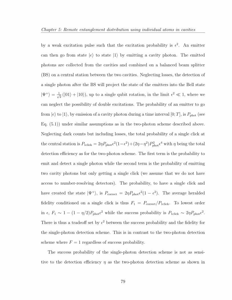
Chapter 5: Remote entanglement distribution using individual atoms in cavities
by a weak excitation pulse such that the excitation probability is ε2. An emitter
can then go from state |e〉 to state |1〉 by emitting a cavity photon. The emitted
photons are collected from the cavities and combined on a balanced beam splitter
(BS) on a central station between the two cavities. Neglecting losses, the detection of
a single photon after the BS will project the state of the emitters into the Bell state
|Ψ+〉 = 1√2
(|01〉+ |10〉), up to a single qubit rotation, in the limit ε2 1, where we
can neglect the possibility of double excitations. The probability of an emitter to go
from |e〉 to |1〉, by emission of a cavity photon during a time interval [0; T ], is Pphot (see
Eq. (5.1)) under similar assumptions as in the two-photon scheme described above.
Neglecting dark counts but including losses, the total probability of a single click at
the central station is P1click = 2ηPphotε2(1−ε2)+(2η−η2)P 2
photε4 with η being the total
detection efficiency as for the two-photon scheme. The first term is the probability to
emit and detect a single photon while the second term is the probability of emitting
two cavity photons but only getting a single click (we assume that we do not have
access to number-resolving detectors). The probability, to have a single click and
have created the state |Ψ+〉, is Pcorrect = 2ηPphotε2(1 − ε2). The average heralded
fidelity conditioned on a single click is thus F1 = Pcorrect/P1click. To lowest order
in ε, F1 ∼ 1 − (1 − η/2)Pphotε2 while the success probability is P1click ∼ 2ηPphotε
2.
There is thus a tradeoff set by ε2 between the success probability and the fidelity for
the single-photon detection scheme. This is in contrast to the two-photon detection
scheme where F = 1 regardless of success probability.
The success probability of the single-photon detection scheme is not as sensi-
tive to the detection efficiency η as the two-photon detection scheme as shown in
79

Chapter 5: Remote entanglement distribution using individual atoms in cavities
Fig. 5.6. If the detection efficiency η is large, the two-photon scheme is desirable
since it will have both a high success probability and a high fidelity. However, if η
is small, the single-photon scheme will be advantageous since it has a relatively high
success probability. Due to the possible high success probability but limited fidelity
of the single-photon scheme, it might be desirable to combine it with entanglement
purification to increase the final fidelity. In this way, the higher success probability
of the single-photon scheme may compensate the lower fidelity. We have therefore
considered the possibility of initial entanglement purification in repeaters based on
the single-photon detection scheme as described below.
5.3.2 Initial purification
Based on a detailed analysis of the various errors that limit the fidelity for the
single-photon scheme including dark counts of the detectors (see App. D.1 for details),
we find that the purification protocol of Ref. [18] effectively corrects for the errors in
the single-photon scheme and we assume that this is used for the initial purification.
However, as pointed out in Ref. [158] an improved fidelity, at the expense of a factor
of ∼ 2 in the success probability, can be obtained by only accepting outcomes where
the two heralding qubits are found in state |1〉|1〉 instead of also accepting |0〉|0〉
outcomes. We will also consider this modification to the purification protocol of
Ref. [18]. The protocol relies on a CNOT operation, which we assume to be made with
the same gate used to perform the subsequent entanglement swapping (see below). To
reflect the most realistic near-term quantum repeaters we consider at most 4 qubits
per repeater stations. We therefore assume that the purification is performed in a
80
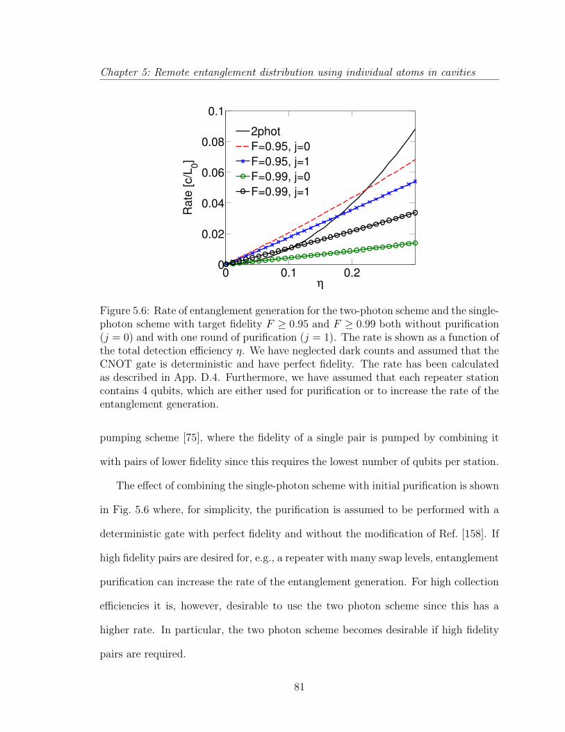
Chapter 5: Remote entanglement distribution using individual atoms in cavities
0 0.1 0.20
0.02
0.04
0.06
0.08
0.1
η
Rate
[c/L
0]
2phot
F=0.95, j=0
F=0.95, j=1
F=0.99, j=0
F=0.99, j=1
Figure 5.6: Rate of entanglement generation for the two-photon scheme and the single-photon scheme with target fidelity F ≥ 0.95 and F ≥ 0.99 both without purification(j = 0) and with one round of purification (j = 1). The rate is shown as a function ofthe total detection efficiency η. We have neglected dark counts and assumed that theCNOT gate is deterministic and have perfect fidelity. The rate has been calculatedas described in App. D.4. Furthermore, we have assumed that each repeater stationcontains 4 qubits, which are either used for purification or to increase the rate of theentanglement generation.
pumping scheme [75], where the fidelity of a single pair is pumped by combining it
with pairs of lower fidelity since this requires the lowest number of qubits per station.
The effect of combining the single-photon scheme with initial purification is shown
in Fig. 5.6 where, for simplicity, the purification is assumed to be performed with a
deterministic gate with perfect fidelity and without the modification of Ref. [158]. If
high fidelity pairs are desired for, e.g., a repeater with many swap levels, entanglement
purification can increase the rate of the entanglement generation. For high collection
efficiencies it is, however, desirable to use the two photon scheme since this has a
higher rate. In particular, the two photon scheme becomes desirable if high fidelity
pairs are required.
81
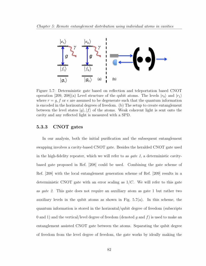
Chapter 5: Remote entanglement distribution using individual atoms in cavities
!!
!
!
g
!
!
! !
!
!
gg
(b) (a)
!!
!
!
g
!
!
! !
!
!
g
(b) (a)
Figure 5.7: Deterministic gate based on reflection and teleportation based CNOToperation [209, 208](a) Level structure of the qubit atoms. The levels |r0〉 and |r1〉where r = g, f or e are assumed to be degenerate such that the quantum informationis encoded in the horizontal degrees of freedom. (b) The setup to create entanglementbetween the level states |g〉, |f〉 of the atoms. Weak coherent light is sent onto thecavity and any reflected light is measured with a SPD.
5.3.3 CNOT gates
In our analysis, both the initial purification and the subsequent entanglement
swapping involves a cavity-based CNOT gate. Besides the heralded CNOT gate used
in the high-fidelity repeater, which we will refer to as gate 1, a deterministic cavity-
based gate proposed in Ref. [208] could be used. Combining the gate scheme of
Ref. [208] with the local entanglement generation scheme of Ref. [209] results in a
deterministic CNOT gate with an error scaling as 1/C. We will refer to this gate
as gate 2. This gate does not require an auxiliary atom as gate 1 but rather two
auxiliary levels in the qubit atoms as shown in Fig. 5.7(a). In this scheme, the
quantum information is stored in the horizontal/qubit degree of freedom (subscripts
0 and 1) and the vertical/level degree of freedom (denoted g and f) is used to make an
entanglement assisted CNOT gate between the atoms. Separating the qubit degree
of freedom from the level degree of freedom, the gate works by ideally making the
82

Chapter 5: Remote entanglement distribution using individual atoms in cavities
transformation
|q1〉|q2〉 ⊗ |gg〉 → |q1〉|q2〉 ⊗ 1√2
(|gf〉+ |fg〉) , (5.6)
where |g〉, |f〉 denote the vertical states and |q1〉 (|q2〉) is the qubit state of the first
(second) qubit, which could be entangled with atoms at neighboring repeater stations.
The entanglement between the levels |g〉 and |f〉 can be used to make a CNOT gate, if
the levels of the atoms can be measured non-destructively, i.e. without revealing any
information about the qubit state as described in Ref. [208]. Both the transformation
shown in Eq. (5.6) and the non-destructive measurements can be obtained by sending
a weak coherent pulse onto a two-sided cavity and detecting any reflected light (see
Fig. 5.7(b) and App. D.3). If the light is resonant with the empty cavity mode,
atoms in |f〉 will shift the cavity resonance. Consequently, photons will be reflected
and constitutes a QND measurement of the presence of atoms in |f〉. Spontaneous
emission from the atoms will limit the fidelity of the gate to F ∼ 1−1.2/(ηdC), where
ηd is the detection efficiency and C = g2/κγ is the cooperativity. The gate time is
limited by the time of the single qubit rotations and the coherent pulses. We assume
that this gives a gate time on the order of 10 µs.
As a benchmark, we also consider a naive approach where a direct gate between
two qubits is made in a cavity without the use of an auxiliary atom or auxiliary atomic
states. To characterize such a gate, we consider a situation where the setup of gate 1
is used to make a deterministic gate by simply ignoring the heralding condition. We
will refer to this gate as gate 3. For such a gate, we find that the gate fidelity will
scale as 1 − F ∼ 3/√C and the time of the gate will be limited by the time of the
single qubit rotations which we assume to be ∼ 10 µs.
83
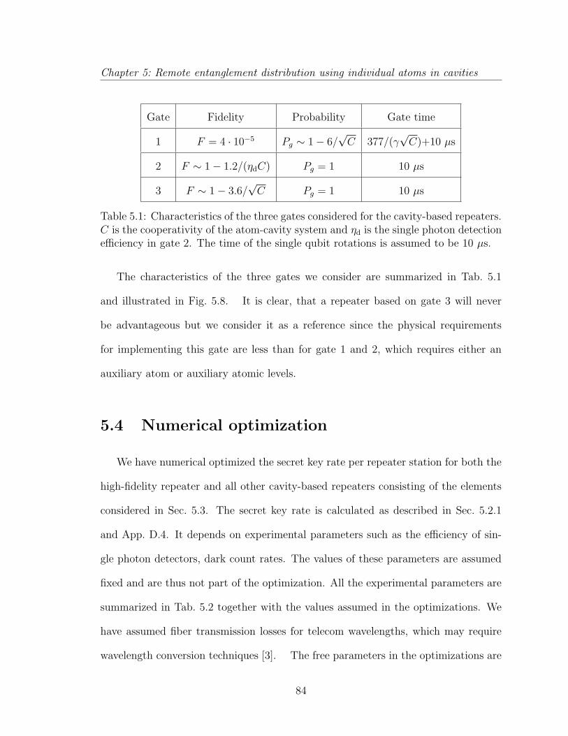
Chapter 5: Remote entanglement distribution using individual atoms in cavities
Gate Fidelity Probability Gate time
1 F = 4 · 10−5 Pg ∼ 1− 6/√C 377/(γ
√C)+10 µs
2 F ∼ 1− 1.2/(ηdC) Pg = 1 10 µs
3 F ∼ 1− 3.6/√C Pg = 1 10 µs
Table 5.1: Characteristics of the three gates considered for the cavity-based repeaters.C is the cooperativity of the atom-cavity system and ηd is the single photon detectionefficiency in gate 2. The time of the single qubit rotations is assumed to be 10 µs.
The characteristics of the three gates we consider are summarized in Tab. 5.1
and illustrated in Fig. 5.8. It is clear, that a repeater based on gate 3 will never
be advantageous but we consider it as a reference since the physical requirements
for implementing this gate are less than for gate 1 and 2, which requires either an
auxiliary atom or auxiliary atomic levels.
5.4 Numerical optimization
We have numerical optimized the secret key rate per repeater station for both the
high-fidelity repeater and all other cavity-based repeaters consisting of the elements
considered in Sec. 5.3. The secret key rate is calculated as described in Sec. 5.2.1
and App. D.4. It depends on experimental parameters such as the efficiency of sin-
gle photon detectors, dark count rates. The values of these parameters are assumed
fixed and are thus not part of the optimization. All the experimental parameters are
summarized in Tab. 5.2 together with the values assumed in the optimizations. We
have assumed fiber transmission losses for telecom wavelengths, which may require
wavelength conversion techniques [3]. The free parameters in the optimizations are
84
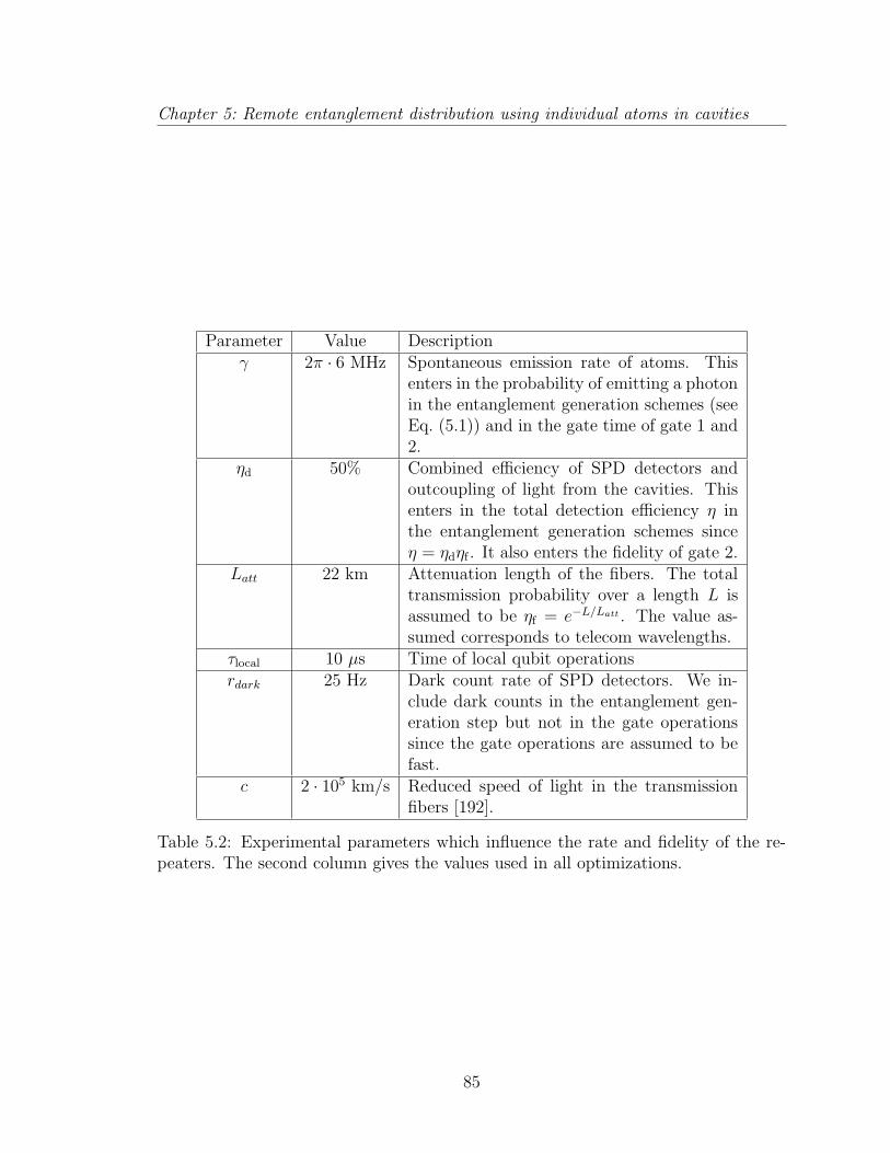
Chapter 5: Remote entanglement distribution using individual atoms in cavities
Parameter Value Descriptionγ 2π · 6 MHz Spontaneous emission rate of atoms. This
enters in the probability of emitting a photonin the entanglement generation schemes (seeEq. (5.1)) and in the gate time of gate 1 and2.
ηd 50% Combined efficiency of SPD detectors andoutcoupling of light from the cavities. Thisenters in the total detection efficiency η inthe entanglement generation schemes sinceη = ηdηf . It also enters the fidelity of gate 2.
Latt 22 km Attenuation length of the fibers. The totaltransmission probability over a length L isassumed to be ηf = e−L/Latt . The value as-sumed corresponds to telecom wavelengths.
τlocal 10 µs Time of local qubit operationsrdark 25 Hz Dark count rate of SPD detectors. We in-
clude dark counts in the entanglement gen-eration step but not in the gate operationssince the gate operations are assumed to befast.
c 2 · 105 km/s Reduced speed of light in the transmissionfibers [192].
Table 5.2: Experimental parameters which influence the rate and fidelity of the re-peaters. The second column gives the values used in all optimizations.
85

Chapter 5: Remote entanglement distribution using individual atoms in cavities
100 101 102 1030.1
0.2
0.4
0.60.8
1
C
Erro
r (ga
te 3
) & 1
−Pg (g
ate
1)
10−3
10−2
10−1
100
Erro
r (ga
te 2
)
1−F, Gate 21−Pg, Gate 11−F, Gate 3
Figure 5.8: Characteristics of the three gates described in the text. The errors of gate2 (black/solid line, right axis) and gate 3 (black/circled line, left axis) are shown as afunction of the cooperativity. The error is defined as 1− F where F is the fidelity ofthe gate. We have assumed ηd = 0.5 for the error of gate 2. Gate 1 has conditionalfidelity ∼ 1 but a finite failure probability 1 − Pg which is also shown as a functionof cooperativity (red/dashed line, left axis).
the number of swap levels, the number of purifications with/without the modification
of Ref. [158] and whether a parallel or sequential repeater protocol is used. In the op-
timizations, we calculate the secret key rate on a grid of all these parameters and pick
the combination giving the highest rate. Fig. 5.9 shows a specific example where the
combination of the single-photon scheme with gate 2 is investigated for a parallel re-
peater and a cooperativity of 100. The number of swap levels and purifications, giving
the highest rate for a specific distance, can be directly read off from the figure. The
same calculations are then done for a sequential repeater protocol and compared to
the parallel repeater protocol with/without the modified purification in order to find
the highest rate for this specific combination of entanglement generation scheme and
CNOT gate. This is done for all combinations of entanglement generation schemes
86
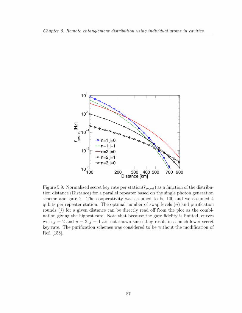
Chapter 5: Remote entanglement distribution using individual atoms in cavities
100 200 300 400 500 700 90010−3
10−2
10−1
100
101
Distance [km]
r secr
et [H
z]
n=1,j=0n=1,j=1n=2,j=0n=2,j=1n=3,j=0
~
Figure 5.9: Normalized secret key rate per station(rsecret) as a function of the distribu-tion distance (Distance) for a parallel repeater based on the single photon generationscheme and gate 2. The cooperativity was assumed to be 100 and we assumed 4qubits per repeater station. The optimal number of swap levels (n) and purificationrounds (j) for a given distance can be directly read off from the plot as the combi-nation giving the highest rate. Note that because the gate fidelity is limited, curveswith j = 2 and n = 3, j = 1 are not shown since they result in a much lower secretkey rate. The purification schemes was considered to be without the modification ofRef. [158].
87
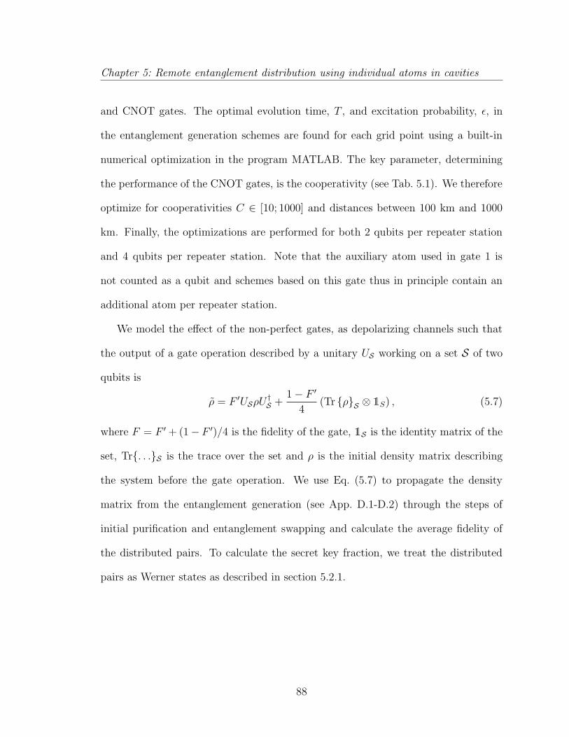
Chapter 5: Remote entanglement distribution using individual atoms in cavities
and CNOT gates. The optimal evolution time, T , and excitation probability, ε, in
the entanglement generation schemes are found for each grid point using a built-in
numerical optimization in the program MATLAB. The key parameter, determining
the performance of the CNOT gates, is the cooperativity (see Tab. 5.1). We therefore
optimize for cooperativities C ∈ [10; 1000] and distances between 100 km and 1000
km. Finally, the optimizations are performed for both 2 qubits per repeater station
and 4 qubits per repeater station. Note that the auxiliary atom used in gate 1 is
not counted as a qubit and schemes based on this gate thus in principle contain an
additional atom per repeater station.
We model the effect of the non-perfect gates, as depolarizing channels such that
the output of a gate operation described by a unitary US working on a set S of two
qubits is
ρ = F ′USρU†S +
1− F ′4
(Tr ρS ⊗ 1S) , (5.7)
where F = F ′ + (1− F ′)/4 is the fidelity of the gate, 1S is the identity matrix of the
set, Tr. . .S is the trace over the set and ρ is the initial density matrix describing
the system before the gate operation. We use Eq. (5.7) to propagate the density
matrix from the entanglement generation (see App. D.1-D.2) through the steps of
initial purification and entanglement swapping and calculate the average fidelity of
the distributed pairs. To calculate the secret key fraction, we treat the distributed
pairs as Werner states as described in section 5.2.1.
88
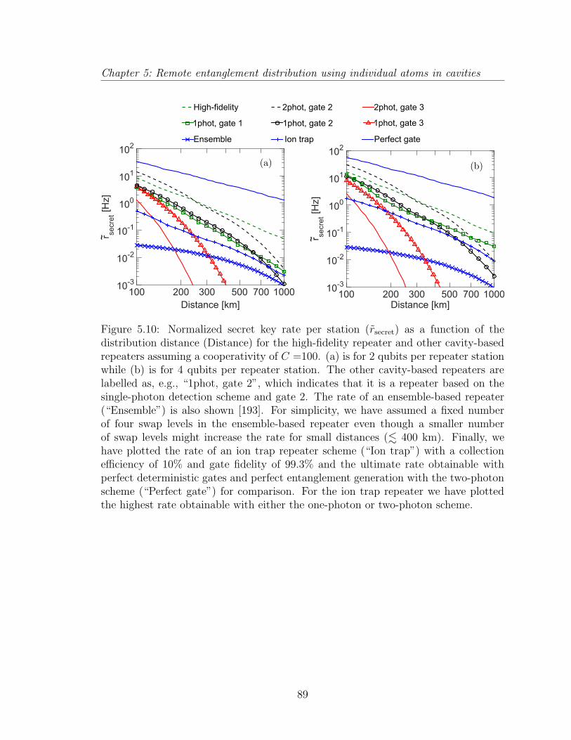
Chapter 5: Remote entanglement distribution using individual atoms in cavities
Figure 5.10: Normalized secret key rate per station (rsecret) as a function of thedistribution distance (Distance) for the high-fidelity repeater and other cavity-basedrepeaters assuming a cooperativity of C =100. (a) is for 2 qubits per repeater stationwhile (b) is for 4 qubits per repeater station. The other cavity-based repeaters arelabelled as, e.g., “1phot, gate 2”, which indicates that it is a repeater based on thesingle-photon detection scheme and gate 2. The rate of an ensemble-based repeater(“Ensemble”) is also shown [193]. For simplicity, we have assumed a fixed numberof four swap levels in the ensemble-based repeater even though a smaller numberof swap levels might increase the rate for small distances (. 400 km). Finally, wehave plotted the rate of an ion trap repeater scheme (“Ion trap”) with a collectionefficiency of 10% and gate fidelity of 99.3% and the ultimate rate obtainable withperfect deterministic gates and perfect entanglement generation with the two-photonscheme (“Perfect gate”) for comparison. For the ion trap repeater we have plottedthe highest rate obtainable with either the one-photon or two-photon scheme.
89
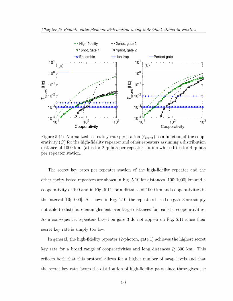
Chapter 5: Remote entanglement distribution using individual atoms in cavities
Figure 5.11: Normalized secret key rate per station (rsecret) as a function of the coop-erativity (C) for the high-fidelity repeater and other repeaters assuming a distributiondistance of 1000 km. (a) is for 2 qubits per repeater station while (b) is for 4 qubitsper repeater station.
The secret key rates per repeater station of the high-fidelity repeater and the
other cavity-based repeaters are shown in Fig. 5.10 for distances [100; 1000] km and a
cooperativity of 100 and in Fig. 5.11 for a distance of 1000 km and cooperativities in
the interval [10; 1000]. As shown in Fig. 5.10, the repeaters based on gate 3 are simply
not able to distribute entanglement over large distances for realistic cooperativities.
As a consequence, repeaters based on gate 3 do not appear on Fig. 5.11 since their
secret key rate is simply too low.
In general, the high-fidelity repeater (2-photon, gate 1) achieves the highest secret
key rate for a broad range of cooperativities and long distances & 300 km. This
reflects both that this protocol allows for a higher number of swap levels and that
the secret key rate favors the distribution of high-fidelity pairs since these gives the
90

Chapter 5: Remote entanglement distribution using individual atoms in cavities
highest secret fraction (see Fig. 5.4). It is also apparent from Fig. 5.11 that while
repeaters based on gate 2 need cooperativities above 100 for a distance of 1000 km,
repeaters based on gate 1 are able to function with much lower cooperativities around
30 − 40. This is because the heralded gate has nearly unit fidelity, independent of
the cooperativity. For high cooperativities or low distances, a repeater based on the
two-photon detection scheme and gate 2 can give a slightly higher secret key rate
than the high-fidelity repeater. This improvement is, however, less than a factor of
2 in the secret key rate. The steps in the rates of the schemes based on gate 2 in
Fig. 5.11 originate from the fact that as the cooperativity increases, the fidelity of gate
2 increases and at some point the fidelity is high enough to allow for another swap
level, which makes the rate increase abruptly. From the optimizations, we find that
the sequential repeater architecture achieves slightly higher rates (less than a factor
2) than the parallel repeater architecture for 4 qubits per repeater station, while the
opposite is the case for 2 qubits per repeater station.
In general, repeaters based on the two-photon detection schemes outperform re-
peaters based on the single-photon detection scheme except for repeaters based on
gate 3. This reflects that repeaters based on gate 3 cannot perform many swap lev-
els since the fidelity simply decreases too rapidly with the number of swap levels.
The result of the optimization was that no swap levels were actually preferred for
repeaters based on gate 3 for C ≤ 1000. As a result, the elementary links in these
repeaters are long and fiber losses therefore significantly decrease the total detection
probability η in the entanglement generation schemes. In the limit of very low η,
the one-photon scheme is advantageous since the success probability only depends
91
Chapter 5: Remote entanglement distribution using individual atoms in cavities
linearly on η. For the optimizations, we have assumed that the combined efficiency
of the SPD detectors and outcoupling of light from the cavities is ηd =50%. If this
efficiency is smaller, repeaters based on single-photon detection may be desirable. We
also find that the purification protocol, in general, performs better with than without
the modification of Ref. [158]. The improvement is, however, limited to a factor of
. 2 for the parameters considered in Figs. 5.10-5.11.
It is important to stress that the rates plotted in Figs. 5.10-5.11 are the secret
key rates divided by the total number of repeater stations. The actual distribution
rate can thus be obtained by multiplying with the number of repeater stations. For
the high-fidelity repeater, we find a secret key rate of ∼16 Hz over 1000 km for 33
repeater stations and a cooperativity of 1000 assuming 2 qubits per repeater station.
For a more modest cooperativity of 100, a secret key rate of ∼1.5 Hz over 1000 km
can be obtained.
We can compare the rate found here to the rate obtainable with repeaters based
on atomic ensembles. In Ref. [193] an efficient repeater based on atomic ensembles
is described, which achieves one of the highest distribution rates for repeaters based
on atomic ensembles [192]. The fidelity of the distributed pair and the distribution
rate are derived in Ref. [193] for a repeater with four swap levels corresponding to
17 repeater stations. Based on this, we have calculated the secret key rate assuming
an optimistic, basic repetition rate of the ensembles of 100 MHz and memory and
SPD efficiencies of 90%. The rate of the ensemble-based repeater is also shown in
Figs. 5.10-5.11 for similar assumptions about fiber losses etc. as for the cavity-based
repeaters. We have assumed that the repeater uses four swap levels for all distances
92
Chapter 5: Remote entanglement distribution using individual atoms in cavities
even though a smaller number of swap levels may be desirable for smaller distances
(. 400 km) [193]. For a distance of 1000 km, we find a rate of ∼ 0.03 Hz for 33
repeater stations. This shows that repeaters based on individual atoms in cavities
may be very promising candidates for realizing efficient quantum repeaters with rates
exceeding those obtainable with atomic ensembles. The main reason for this is that
very efficient entanglement swapping can be realized in the cavity-based repeaters
which greatly enhances the distribution rates for long distances. On the contrary,
repeaters based on atomic ensembles and linear optics have an upper limit on the
swapping efficiency of 50%.
For comparison we have also considered a repeater based on ion traps where
there is no cavity to collect the light. Non-local entanglement can still be created by
collecting the emitted light with a lens as demonstrated in Ref. [109] where a collection
efficiency of 10% was reported. The entanglement swapping can be realized using a
gate, which has been demonstrated experimentally with a fidelity of 99.3% and a gate
time of 50 µs [16]. Note that this fidelity was measured for the generation of a single
state in Ref. [16] but we will assume it to be the fidelity of the entanglement swap. The
rate of such a ion-trap repeater is shown in Figs. 5.10-5.11 with assumptions about
fiber losses etc. summarized in Tab. 5.2. We have assumed a collection efficiency
of 10% and as a result, the one photon scheme with modified purification performs
better than the two-photon scheme for 4 qubits per repeater station. However for
two qubits, where purification is not possible, the two-photon scheme is in general
advantageous except for small distances (< 200 km). We have assumed a gate fidelity
of 99.3% and have plotted the highest rate obtainable with either the one-photon or
93
Chapter 5: Remote entanglement distribution using individual atoms in cavities
two-photon scheme.
It is seen that the high-fidelity repeater outperforms the ion-trap repeater for C &
30, which is mainly due to the low collection efficiency in the entanglement generation.
The ultimate rate, obtainable with a repeater with perfect deterministic entanglement
swapping and entanglement generation based on the two-photon detection scheme
with a collection efficiency set by 4C/(1 + 4C), is also shown in Figs. 5.10-5.11. A
similar repeater was considered in Ref. [191] to demonstrate the feasibility of repeaters
based on trapped ions. For C = 1000, the high-fidelity repeater achieves only a factor
of ∼ 2 slower rate than this ultimate limit for a distance of 1000 km.
5.5 Conclusion
In conclusion, we have performed a detailed analysis of quantum repeaters based
on individual emitters in optical cavities. We have found that a high-fidelity repeater
based on the heralded gate described in Ref. [26] combined with a two-photon detec-
tion scheme is the best option over a large parameter regime and enables high secret
key rates over large distances even for limited cooperativities < 100. Compared with
a number of other cavity based repeaters it achieves rates that are up to two orders of
magnitude faster for long distances (1000 km) and cooperativities < 100. For small
distances or higher cooperativities, a repeater based on the deterministic CNOT gate
described in Ref. [208] combined with a two-photon detection scheme can achieve
rates which are slightly higher than the high-fidelity repeater but the improvement is
less than a factor of 2.
We have also compared the high-fidelity repeater to the repeater in Ref. [193],
94
Chapter 5: Remote entanglement distribution using individual atoms in cavities
which is based on atomic ensembles. For a distance of 1000 km and C & 20 the
high-fidelity repeater begins to outperform the ensemble-based repeater and an im-
provement of more than two orders of magnitude in the secret key rate is possible
for C & 100. The main reason for the advantage of the high-fidelity repeater is
that entanglement can be swapped very efficiently using the heralded CNOT gate
described in Ref. [26]. Consequently, the number of swap levels in the repeater can
be increased without the need of intermediate purification, which greatly enhances
the rate for large distances. A similar advantage could in principle be achieved by
resorting to a trapped ion system, where efficient gates can be implemented. For
current systems, the collection efficiencies are, however, so low that a trapped ion
system could be outperformed by a cavity system with a limited finesse of C & 30. If
the collection efficiency could be overcome, e.g. by placing the ions in a cavity with
a high cooperativity, the rate can be substantially improved, but with C > 1000 the
high fidelity repeater investigated here is within a factor of two of this ideal repeater.
It should, however, be noted that we have compared schemes with strong physical
differences in our analysis. The high-fidelity repeater requires an extra auxiliary atom
while auxiliary atomic levels are required to decrease the error of the deterministic
cavity-based CNOT gates. The ensemble-based and ion-trap repeaters are also very
different physical systems compared to the cavity-based repeaters with individual
atoms. The different experimental difficulties in realizing the physical requirements
for the various repeater schemes should be included in a more advanced assessment.
Finally, we note that while we have investigated a number of different possible
repeater protocols there may be even more advantageous procedures. Hence the
95
Chapter 5: Remote entanglement distribution using individual atoms in cavities
results that we have derived here should be seen as lower limits to the achievable
communication rates. A particular interesting possibility could be to investigate
proposals along the lines of Ref. [228, 227], which also rely on heralding measurements
to detect errors during entanglement generation and two qubit operations. Possibly
some of the ideas from these schemes could be used to improve the communication
beyond what we have found here.
96

Chapter 6
Heisenberg-Limited Atom Clocks
Based on Entangled Qubits
6.1 Introduction
Currently, atomic clocks based on optical transitions achieve the most precise [156,
23, 126] and accurate [52, 23] frequency references. Additionally, the development of
optical frequency combs [78, 176, 114, 240] – establishing a coherent link between the
optical and radio frequencies – enabled the application of optical frequency standards
to a wide range of scientific and technological fields including astronomy, molecular
spectroscopy and global positioning systems.
The improvement of frequency standards using quantum resources, such as entan-
glement [38, 6, 130, 184, 28], has been actively explored in recent years. While clock
protocols based on uncorrelated atoms at best achieve a stability scaling ∝ 1/√N ,
where N is the number of atoms – a scaling commonly known as the standard quan-
97
Chapter 6: Heisenberg-Limited Atom Clocks Based on Entangled Qubits
tum limit (SQL) [41] – the use of entangled resources, in principle, allows one to
surpass this limit. However, a characterization of the improvement obtainable by
using entanglement requires a detailed investigation of the decoherence present in the
system. Previous studies have focused on two kind of noise sources: i) single particle
decoherence resulting from the interaction of the atoms with the environment and
ii) frequency fluctuations in the laser used to excite the clock transition [in the fol-
lowing also referred to as local oscillator (LO)]. It is well known that fully entangled
states (e.g., Greenberger-Horne-Zeilinger (GHZ) states) allow for improved spectro-
scopic sensitivity, but in the same way that these states benefit from their increased
sensitivity in the laser interrogation, they are generally prone to various types of
noise sources canceling any quantum gain. It has therefore been long believed that
such states fail to increase clock stability regardless of the noise model being used
[24, 237, 184, 110]. On the other hand, it has been shown that for clocks with local
oscillator noise limited stability, the use of moderately squeezed atomic states can
yield a modest improvement over the SQL [6, 130]. A recent study demonstrated
further that, in principle, highly squeezed states could achieve Heisenberg-limited
stability (i.e., a 1/N scaling with the available resources representing the ultimate
limit allowed by the laws of quantum mechanics [95]) using a complex adaptive mea-
surement scheme [28]. At the same time, it has been shown that the single particle
decoherence-limited regime can be reached for long averaging time at a logarithmic
cost in N by interrogating uncorrelated atomic ensembles for suitably chosen times
[183, 27].
In this chapter, we introduce a protocol involving groups of sequentially larger
98
Chapter 6: Heisenberg-Limited Atom Clocks Based on Entangled Qubits
GHZ states to estimate local oscillator deviations from the atomic reference in a
manner reminiscent of the phase estimation algorithm [159]. Furthermore, we unify
previous treatments of decoherence for atomic clocks and incorporate previous pro-
posals involving uncorrelated atoms to effectively narrow the LO linewidth [183, 27]
and thereby identify ultimate limits to the stability of atomic clocks based on entan-
gled atoms. We find that for LO-noise limited clocks, the proposed quantum protocol
is found to be nearly optimal, realizing the Heisenberg limit of clock stability up to
a logarithmic correction in the particle number. Importantly, it reaches the funda-
mental noise floor resulting from individual dephasing of the clock qubits N times
faster than the best known classical schemes, where N is the total number of particles
employed.
The central idea of our approach can be understood as follows. In modern atomic
clocks, the frequency of a LO is locked to an ultra-narrow transition of the clock
atoms serving as the frequency reference. The long-term stability of such a clock
after a given total averaging time τ is directly related to the precision by which the
accumulated laser phase relative to the atoms can be determined. To this end, the
phase is repeatedly measured in a standard Ramsey protocol [174]: Using the LO, the
clock qubits are prepared in a superposition of |1〉 and |0〉, denoting the levels of the
clock transition. After the qubits evolve freely for a time T (Ramsey interrogation
time), they are subsequently measured in an orthogonal basis (|±〉 ≡ |1〉±|0〉), which
yields an estimate of the accumulated phase difference between the LO and the atomic
frequency reference. It is known, that since each of these Ramsey sequences introduces
measurement noise, it is optimal to extend the Ramsey time T to its maximum value
99
Chapter 6: Heisenberg-Limited Atom Clocks Based on Entangled Qubits
T → τ [30].
A single GHZ state consisting of N entangled atoms – whose state after the
interrogation is |GHZ〉T ∝ |0〉⊗N + exp(−iNΦLO)|1〉⊗N – accumulates the laser phase
(denoted by ΦLO) N times faster than an uncorrelated state, allowing a more precise
phase measurement [95]. However, fluctuations in the laser frequency renders the laser
phase a random variable with a probability distribution that grows in width as we
increase the Ramsey time T . Whenever the laser phase realized in a particular Ramsey
cycle induces a full phase wrap on the state [i.e., the atomic phase NΦLO /∈ [−π, π)],
a subsequent measurement yields a 2π error in the estimation. For a single GHZ
state, this accounts for a strict limitation on the maximally allowed Ramsey time in
order to limit the initial variance of ΦLO, and the resulting laser stability is found to
yield no improvement over classical protocols [237].
To address this problem, we use a protocol involving an incoherent version of
the phase estimation algorithm [159], similar to the one outlined in [94] but adapted
to be applicable also when the frequency fluctuates and phases exceed 2π. The
phase estimation algorithm has recently been successfully applied experimentally for
global interferometric phase estimation [105, 152], and its use in clock synchronization
protocols has been discussed [59]. Here, we demonstrate how the same techniques can
be applied to guarantee optimal laser stability by allowing the Ramsey interrogation
time to be extended to its maximum value.
Let us assume, for the moment, that the accumulated laser phase after the inter-
rogation time T lies in the interval ΦLO ∈ [−π, π), and has an exact binary represen-
tation (ΦLO + π)/2π =∑M
j=1 Zj/2j, with digits Zj ∈ 0, 1 (both conditions will be
100
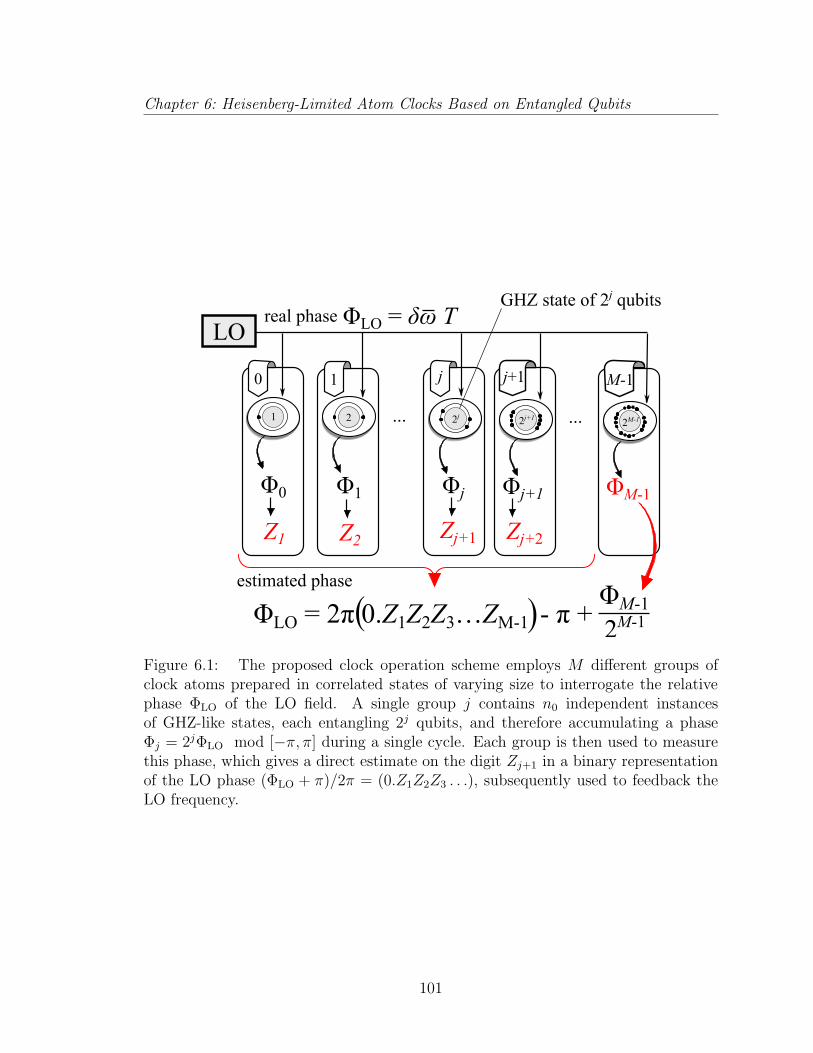
Chapter 6: Heisenberg-Limited Atom Clocks Based on Entangled Qubits
Figure 6.1: The proposed clock operation scheme employs M different groups ofclock atoms prepared in correlated states of varying size to interrogate the relativephase ΦLO of the LO field. A single group j contains n0 independent instancesof GHZ-like states, each entangling 2j qubits, and therefore accumulating a phaseΦj = 2jΦLO mod [−π, π] during a single cycle. Each group is then used to measurethis phase, which gives a direct estimate on the digit Zj+1 in a binary representationof the LO phase (ΦLO + π)/2π = (0.Z1Z2Z3 . . .), subsequently used to feedback theLO frequency.
101
Chapter 6: Heisenberg-Limited Atom Clocks Based on Entangled Qubits
relaxed below). One can then readily show that a GHZ state consisting of 2M−1 atoms
picks up the phase ΦM−1 = 2M−1ΦLO mod [−π, π) = π(ZM − 1). Thus, by measuring
if the phase is 0 or π, the last digit of the laser phase can be determined. However,
without the remaining digits this information is useless. In our protocol, these digits
are found by an additional, simultaneous interrogation with successively smaller GHZ
states of 2M−2, 2M−3, . . . entangled atoms (see Fig. 6.1). Each of these states picks
up a phase proportional to its size, Φj = 2jΦLO mod [−π, π), and this phase gets a
contribution of π(Zj−1). By distinguishing whether the phase is shifted by π or not,
we can determine the value of the bit Zj. The combined information provides an esti-
mate with an accuracy given by the largest GHZ state, while the cascade increases the
total number of atoms employed only by a factor of two:∑M−1
j=0 2j ≈ 2M = 2× 2M−1.
However, in the limit of large averaging times, the assumption ΦLO ∈ [−π, π) is
not justified anymore. Here, the optimal Ramsey time T ∼ τ can attain values that
induce phase wraps of the laser itself, causing the binary representation of the laser
phase to contain digits Zj 6= 0 for j ≤ 0, which are inaccessible to the technique dis-
cussed above. To overcome this, we extend the cascade to the classical domain, and
employ additional groups of uncorrelated atoms that interrogate the laser with suc-
cessively decreasing interrogation times, or alternatively, using dynamical decoupling
techniques [183, 27, 225]. Each of these ensembles acquires a phase that is reduced
by multiples of two from the laser phase, and thus, following the arguments from
above, allows one to gain information on the digits Zj with j ≤ 0. The information
of all digits combined provides the total number of phase wraps, which in turn yields
a Heisenberg-limited estimate of the laser phase. By this, the protocol effectively
102
Chapter 6: Heisenberg-Limited Atom Clocks Based on Entangled Qubits
eliminates all limitations arising from the LO noise, and allows the Ramsey time to
extend to its optimal value.
6.2 Feedback loop
In the following, we provide a derivation of the above results combined with feed-
back analysis that allows us to characterize the achievable stability of a clock using
our protocol. Modern clocks periodically measure the fluctuating LO frequency ω(t)
against the frequency standard ω0 of the clock atoms to obtain an error signal. After
each Ramsey cycle of duration T [i.e., at times tk = kT (k = 1, 2 . . .)], the mea-
surement data yield an estimate of the relative phase, ΦLO(tk) =∫ tktk−T
dt [ω(t)− ω0],
accumulated by the LO. This estimate in turn is used to readjust the frequency of
the LO: ω(tk)→ ω(tk)−αΦestLO(tk)/T , where Φest
LO(tk) represents a suited estimator of
the phase ΦLO(tk)1, and α < 1 is a suitably chosen gain.
The stability of the actively stabilized LO, after a total averaging time τ , is char-
acterized by the Allan deviation (ADEV) which is directly proportional to the mea-
surement uncertainty ∆ΦLO(tk) after each Ramsey cycle (see Appendix E.1),
σy(τ) ≡ 1
ω0τ
√√√√τ/T∑
k=1
τ/T∑
l=1
T 2 〈δωkδωl〉 ≈1
ω0
√τT
∆ΦLO(T ). (6.1)
Here, δωk = ΦLO(tk)/T is the average detuning of the (stabilized) LO during the
kth cycle. To obtain Eq. 6.1, we use the fact that after the frequency feedback
the detuning averages become approximately uncorrelated for realistic laser spectra,
〈δωkδωl〉 ≈ 〈δω2〉 δkl [27, 7, 23]. Other noise sources (such as the bias of the linear
1Alternatively, it is also possible to perform direct phase feedback.
103
Chapter 6: Heisenberg-Limited Atom Clocks Based on Entangled Qubits
estimator, the Dick effect, or a sub-optimal gain α [194]) are not fundamental, and
neglected in the following.
6.3 Spectroscopic noises
For small values of the accumulated Ramsey phase, the ultimate precision by which
this phase can be estimated is determined by the Cramer-Rao bound [57, 95] which
links the estimation error to the quantum Fisher information (QFI) ∆ΦLO ∼ 1/√F
(for a review, see [95]). The QFI, F , is maximized, e.g., by the use of GHZ states for
which F ∼ N2. In clock stabilization, however, the LO frequency fluctuations account
for the fact that the accumulated Ramsey phase is a random variable which can
obtain large values, inherently violating the small phase assumption of the Cramer-
Rao bound. In particular for a single GHZ states, phase wraps of the atomic phase,
Φ(tk) = NΦLO(tk) /∈ [−π, π), cannot be detected. Consequently, the cycle time T
has to be chosen such that the prior distribution of Φ(tk) is well localized within
[−π, π). This limits the maximally allowed Ramsey time to a value Tmax ∼ γ−1LO/N
2
(see Appendix E.3), where we assumed a white frequency noise spectrum of the LO,
Sω(f) = γLO (for 1/f -noise one finds the less stringent condition Tmax ∼ γ−1LO/N). In
most cases, this value lies below the optimal (i.e., maximal) value implied by Eq. 6.1
T ∼ τ , resulting in a laser stability for GHZ states which shows no improvement over
the stability achieved with uncorrelated atoms [237, 184].
However, unlike the individual particle noise resulting in the finite atom linewidth
γind, the LO frequency fluctuations affect all clock atoms alike, and this collective noise
does not represent a fundamental metrological limitation. We can use a cascade of
104
Chapter 6: Heisenberg-Limited Atom Clocks Based on Entangled Qubits
GHZ states of varying size to measure the ΦLO in a binary representation, as discussed
above. In general, the phase does not have an exact binary representation ending at
the digit ZM . We therefore employ n0 duplicates at each level of the cascade (as
opposed to sequential procedure suggested in [94]) (n0 = N/∑M−1
j=0 2j ≈ N/2M) to
improve the precision. In the case where all digits Zj (j = 1 . . . ,M−1) are determined
correctly according to the relation
Zj = [2(Φj−1 + π)− (Φj + π)]/2π, (6.2)
the last group (j = M −1) then yields a Heisenberg-limited estimate of the LO phase
with accuracy (∆ΦLO)pr = 1/(2M−1√n0) = 2√n0/N .
6.3.1 Phase estimation with multiple GHZ groups
However, in general the estimation of the binary digits Zj is not perfect. A
rounding error occurs whenever |Φestj−1−Φj−1| > π/2 (where Φest
j represents a suitable
estimator derived from the n0 measurement outcomes), leading to the wrong Zj, and
a variance contribution of (2π2−j)2 for ΦLO. We can approximate their total variance
contribution with the sum (∆ΦLO)2re = Pre
∑M−1j=1 (2π2−j)2, where Pre = 2
∫∞π/2dφ ρ(φ),
and ρ(φ) is the Gaussian probability distribution of the error Φestj − Φj with a width
proportional to 1/√n0 (see Appendix E.3). Consequently, rounding errors can be
exponentially suppressed by choosing a sufficiently large value for n0. The total
measurement uncertainty of this estimation scheme is thus (∆ΦLO)2 = (∆ΦLO)2pr +
(∆ΦLO)2re. In Appendix E.3, we show that the optimal allocation of resources is
achieved for the choice nopt0 ∼ 16
π2 log (N), for which rounding errors are negligible,
105
Chapter 6: Heisenberg-Limited Atom Clocks Based on Entangled Qubits
yielding the total measurement accuracy
∆ΦLO ≈ (∆ΦLO)pr =8
π
√log(N)/N. (6.3)
This measurement precision obtains the Heisenberg limit (up to a logarithmic correc-
tion resulting from the cost to suppress rounding errors) despite it being applicable
to a general (typically large) phase.
So far we have assumed that ΦLO ∈ [−π, π) in each cycle. However, for realistic
laser noise spectra there is always a finite probability that the LO phase ΦLO lies
outside the interval [−π, π) after the interrogation time. Such phase wraps of the
laser phase itself add to the final measurement uncertainty in Eq. 6.3 by the amount
(∆ΦLO)2slip = (2π)2Pslip, where Pslip = 2
∫∞πdφ ρLO(φ), and ρLO is the Gaussian prior
distribution of ΦLO. Its width grows with γLOT , which puts a constraint on the
maximally allowed Ramsey time T ≤ π2
4γ−1
LO[log(γLOτN)]−1, and thus the achievable
ADEV σy (∝ 1/√T ) as we demonstrate in Appendix E.3.
This, however, does not represent a fundamental limitation as we can extend the
scheme by adding additional classical measurements with a shorter Ramsey periods
to assess the number of phase slips of the laser phase itself . . . Z−3Z−2Z−1Z0. As
demonstrated in Appendix E.3, this allows extending the Ramsey time by a factor k
adding only a negligible number of atoms N∗ ≈ 8π2 log (kN2) log2(k) N .
6.3.2 Optimization
With all phase wraps counted correctly, the Ramsey time is only limited by indi-
vidual noise processes. The finite linewidth of the atomic clock transition γind gives
rise to the fundamental constraint T ≤ γ−1ind/2
M−1. For averaging times τ ≤ γ−1ind/2
M−1,
106
Chapter 6: Heisenberg-Limited Atom Clocks Based on Entangled Qubits
we can choose T ≈ τ , and using the optimized value for n0 found above the resulting
clock stability is obtained from Eq. 6.1
σy(τ)(1) ≈ 2
ω0τ
√nopt
0
N≈ 8
πω0τ
√log(N)
N. (6.4)
It scales linearly with the averaging time τ , and realizes the Heisenberg bound of laser
stability up to a logarithmic correction. In contrast, in the regime τ ≥ γ−1ind/2
M−1,
T is limited by the presence of individual particle noise to a value T ≈ γ−1ind/2
M−1 =
2γ−1indn0/N , and we find
σy(τ)(2) ≈ 1
ω0
√γind
τN. (6.5)
Eq. 6.5 represents the fundamental noise floor for laser stability resulting from quan-
tum metrological bounds in the presence of individual particle noise [82]. As we have
seen, the proposed protocol reaches this optimal value rapidly after the averaging time
τ0 ∼ γ−1indlog(N)/N (cf. Fig. 6.2), N/log(N) times faster than any classical scheme.
In Appendix E.6 we derive the necessary threshold fidelities in the GHZ state prepa-
ration our scheme can tolerate without compromising the stability in Eqs. (6.4) &
(6.5).
6.4 Comparison with other schemes
In the following, we benchmark the stability of our protocol against different
approaches by comparing the lowest achievable ADEV as a function of averaging
time τ (cf. Fig. 6.2). First, we consider the standard procedure in which all atoms
are interrogated in an uncorrelated fashion. The scheme is identical to N independent
measurements of ΦLO, and therefore the ADEV is limited by the standard quantum
107
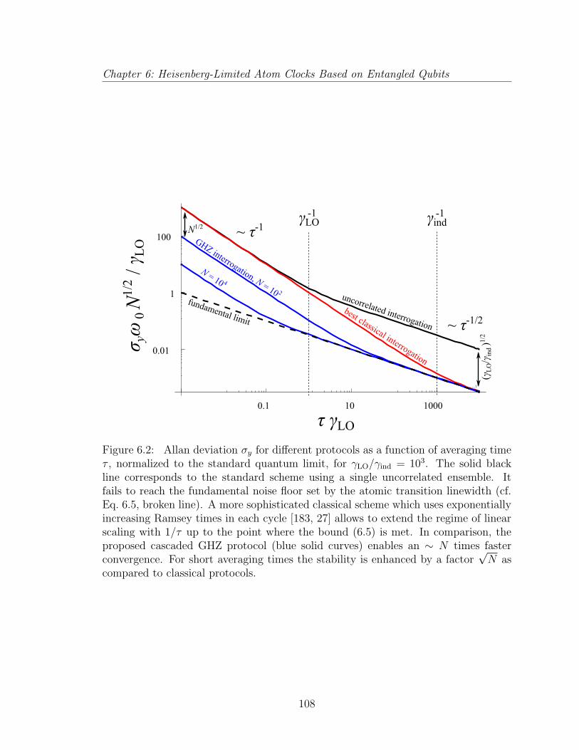
Chapter 6: Heisenberg-Limited Atom Clocks Based on Entangled Qubits
Figure 6.2: Allan deviation σy for different protocols as a function of averaging timeτ , normalized to the standard quantum limit, for γLO/γind = 103. The solid blackline corresponds to the standard scheme using a single uncorrelated ensemble. Itfails to reach the fundamental noise floor set by the atomic transition linewidth (cf.Eq. 6.5, broken line). A more sophisticated classical scheme which uses exponentiallyincreasing Ramsey times in each cycle [183, 27] allows to extend the regime of linearscaling with 1/τ up to the point where the bound (6.5) is met. In comparison, theproposed cascaded GHZ protocol (blue solid curves) enables an ∼ N times fasterconvergence. For short averaging times the stability is enhanced by a factor
√N as
compared to classical protocols.
108
Chapter 6: Heisenberg-Limited Atom Clocks Based on Entangled Qubits
limit: σy ∼ 1ω0τ√N
for τ < γ−1LO. Since the Ramsey time is limited, by the LO noise, to
T < γ−1LO due to uncorrected phase wraps, this fails to achieve the fundamental bound,
Eq. 6.5, giving suboptimal ADEV, σy(τ) ∼ 1ω0
√γLO
τN, in the long time limit τ > γ−1
LO.
Second, we discuss the recently published classical protocol which interrogates the
LO with uncorrelated atoms for exponentially increasing Ramsey times in each cycle
[27, 183]. This protocol can be understood as the classical part (j ≤ 0) of the cascaded
interrogation proposed here . It eliminates the constraint of the LO linewidth, and
allows to extend the interrogation time T to its maximum value, enabling a linear
scaling with τ up to the point where the fundamental bound (6.5) is reached. However,
using an uncorrelated interrogation, the scheme displays a standard-quantum-limited
scaling (i.e. ∝ 1/√N), for short averaging times.
The above analysis illustrates the quantum gain of the proposed clock operation
protocol using cascaded GHZ states. As compared to the best known classical scheme,
our scheme provides a√N/log(N) enhancement for short averaging times. As a
result it reaches the fundamental noise floor for laser stability in the presence of
single particle decoherence [Eq. 6.5] ∼ N/log(N) times faster. This results identifies
the possible advantage of using entanglement previously debated in the literature
[237, 110, 130, 184, 28, 6, 38, 147]: While the long term limitation is set by atomic
decoherence, entangled atoms reaches this limit faster thus improving the bandwidth
of the stable oscillator. Our results motivate the development of quantum enhanced
atomic clocks based on entangled ions and neutral atoms. Furthermore, it lays the
foundations for the recently proposed network of quantum clocks [121] which achieves
the optimal use of resources in a global network through network-wide entangled
109
Chapter 6: Heisenberg-Limited Atom Clocks Based on Entangled Qubits
states.
110
Chapter 7
A quantum network of clocks
7.1 Introduction
The development of precise atomic clocks plays an increasingly important role in
modern society. Shared timing information constitutes a key resource for navigation
with a direct correspondence between timing accuracy and precision in applications
such as the Global Positioning System (GPS). By combining precision metrology and
quantum networks, we propose a quantum, cooperative protocol for operating a net-
work of geographically remote optical atomic clocks. Using non-local entangled states,
we demonstrate an optimal utilization of global resources, and show that such a net-
work can be operated near the fundamental precision limit set by quantum theory.
Furthermore, the internal structure of the network, combined with quantum com-
munication techniques, guarantees security both from internal and external threats.
Realization of such a global quantum network of clocks may allow construction of a
real-time single international time scale (world clock) with unprecedented stability
111
Chapter 7: A quantum network of clocks
and accuracy.
With the advances of highly phase coherent lasers, optical atomic clocks containing
multiple atoms have demonstrated stability that reaches the standard quantum limit
(SQL) set by the available atom number and interrogation time [23, 107, 156]. Reach-
ing beyond the SQL, we stand to gain a significant improvement of clock performance
by preparing atoms in quantum correlated states (e.g., spin squeezed states [127, 38]).
Here we describe a new approach to maximize the performance of a network composed
of multiple clocks allowing one to gain the advantage of all resources available at each
node. Several recent advances in precision metrology and quantum science, along
with future improvements in quantum control, may put this approach within reach.
On the one hand, phase coherent optical links spanning the entire visible spectrum
have been demonstrated, with the capability of delivering the most stable optical os-
cillator from one color or location to another [240, 67]. On the other hand, quantum
communication and entanglement techniques are enabling distant quantum objects to
be connected in a quantum network [54, 117, 169]. Combining these two technologi-
cal frontiers, we show here that a distributed network composed of quantum-limited
clocks separated by large distances – as appropriate, e.g., for satellite-based clocks
possibly operated by different nations – can be operated as an ultimate “world clock”,
where all members combine their individual resources in a quantum coherent way to
achieve greater clock stability and distribute this international time scale in real time
for all.
The distributed architecture allows each participant of the network to profit from a
stability of the local clock signal that is enhanced by a factor proportional to the total
112
Chapter 7: A quantum network of clocks
number of parties (as compared to an independent operation of the individual clocks)
without losing sovereignty or compromising security. This cooperative gain strongly
incentivizes joining the collaborative network while retaining robustness against dis-
ruptions of communication channels. On the one hand, the local clocks can be used
to identify and correct systematic errors originating from the phase links. On the
other hand, the nodes can fall back to relying on the locally stabilized clocks if the
phase links fail. We demonstrate that by preparing quantum-correlated states of re-
mote clocks, the network can yield the best possible clock signal allowed by quantum
theory for the combined resources. Furthermore, enabled through the use of quantum
communication techniques, such a network can be made secure, such that only parties
contributing to its operation may enjoy the benefit of an ultra-precise clock signal.
Besides serving as a real-time clock for the international time scale, the proposed
quantum network also represents a large-scale quantum sensor that can be used to
probe the fundamental laws of physics, including relativity and connections between
space-time and quantum physics.
7.2 The concept of quantum clock network
Fig. 7.1 illustrates the basic concept for the proposed quantum clock network.
We consider a set of K atomic clocks (constituting the nodes of the network), each
based on a large number of atoms (clock qubits) serving as the frequency reference
ω0 at different geographical locations. In our approach, each clock has its own inde-
pendently operated local oscillator (LO), Ej(t) ∝ eiνjt, with detuning δj = νj − ω0,
(j = 1, 2 . . . K). It keeps the time by interrogating its qubits periodically, and uses
113
Chapter 7: A quantum network of clocks
the measurement data to stabilize the LO frequency at the reference frequency of the
atomic transition. However, as opposed to the conventional approach, we consider
the situation in which each network node allocates some of its qubits to form entan-
gled states stretching across all nodes. When interrogated within a properly designed
measurement scheme, such entangled network states provide ultra-precise informa-
tion about the deviation of the center-of-mass (COM) frequency νCOM =∑
j νj/K of
all local oscillators from the atomic resonance.
Each clock cycle consists of three stages: preparation of the clock atom state
(initialization), interrogation by the LOs (measurement) and correction of the laser
frequency according to the measurement outcome (feedback). In the further analysis,
we assume, for convenience, that in each interrogation cycle one of the nodes plays
the role of the center, which initiates each Ramsey cycle and collects the measurement
data from the other nodes via classical channels [Fig. 7.1 b)], as well as LO signals
via optical links, to feedback the COM signal. (The role of the center can alternate
to provide extra security, see Appendix F.2). This information, in turn, can be
utilized in a feedback cycle to yield a Heisenberg-limited stability of the COM clock
signal generated by the network, which is subsequently distributed to the individual
nodes in a secure fashion. As a result, after a few cycles, the LOs corresponding
to each individual node achieve an accuracy and stability effectively resulting from
interrogating atoms in the entire network.
114
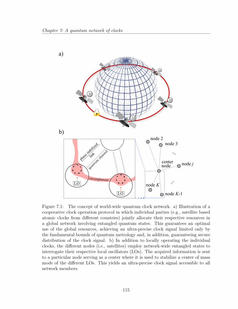
Chapter 7: A quantum network of clocks
Figure 7.1: The concept of world-wide quantum clock network. a) Illustration of acooperative clock operation protocol in which individual parties (e.g., satellite basedatomic clocks from different countries) jointly allocate their respective resources ina global network involving entangled quantum states. This guarantees an optimaluse of the global resources, achieving an ultra-precise clock signal limited only bythe fundamental bounds of quantum metrology and, in addition, guaranteeing securedistribution of the clock signal. b) In addition to locally operating the individualclocks, the different nodes (i.e., satellites) employ network-wide entangled states tointerrogate their respective local oscillators (LOs). The acquired information is sentto a particular node serving as a center where it is used to stabilize a center of massmode of the different LOs. This yields an ultra-precise clock signal accessible to allnetwork members.
115
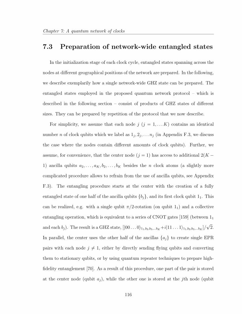
Chapter 7: A quantum network of clocks
7.3 Preparation of network-wide entangled states
In the initialization stage of each clock cycle, entangled states spanning across the
nodes at different geographical positions of the network are prepared. In the following,
we describe exemplarily how a single network-wide GHZ state can be prepared. The
entangled states employed in the proposed quantum network protocol – which is
described in the following section – consist of products of GHZ states of different
sizes. They can be prepared by repetition of the protocol that we now describe.
For simplicity, we assume that each node j (j = 1, . . . K) contains an identical
number n of clock qubits which we label as 1j, 2j, . . . nj (in Appendix F.3, we discuss
the case where the nodes contain different amounts of clock qubits). Further, we
assume, for convenience, that the center node (j = 1) has access to additional 2(K −
1) ancilla qubits a2, . . . , aK , b2, . . . , bK besides the n clock atoms (a slightly more
complicated procedure allows to refrain from the use of ancilla qubits, see Appendix
F.3). The entangling procedure starts at the center with the creation of a fully
entangled state of one half of the ancilla qubits bj, and its first clock qubit 11. This
can be realized, e.g. with a single qubit π/2-rotation (on qubit 11) and a collective
entangling operation, which is equivalent to a series of CNOT gates [159] (between 11
and each bj). The result is a GHZ state, [|00 . . . 0〉11,b2,b3,...bK+i|11 . . . 1〉11,b2,b3,...bK ]/√
2.
In parallel, the center uses the other half of the ancillas aj to create single EPR
pairs with each node j 6= 1, either by directly sending flying qubits and converting
them to stationary qubits, or by using quantum repeater techniques to prepare high-
fidelity entanglement [70]. As a result of this procedure, one part of the pair is stored
at the center node (qubit aj), while the other one is stored at the jth node (qubit
116
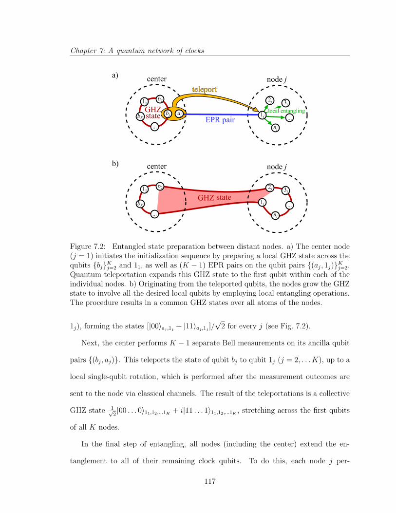
Chapter 7: A quantum network of clocks
Figure 7.2: Entangled state preparation between distant nodes. a) The center node(j = 1) initiates the initialization sequence by preparing a local GHZ state across thequbits bjKj=2 and 11, as well as (K − 1) EPR pairs on the qubit pairs (aj, 1j)Kj=2.Quantum teleportation expands this GHZ state to the first qubit within each of theindividual nodes. b) Originating from the teleported qubits, the nodes grow the GHZstate to involve all the desired local qubits by employing local entangling operations.The procedure results in a common GHZ states over all atoms of the nodes.
1j), forming the states [|00〉aj ,1j + |11〉aj ,1j ]/√
2 for every j (see Fig. 7.2).
Next, the center performs K − 1 separate Bell measurements on its ancilla qubit
pairs (bj, aj). This teleports the state of qubit bj to qubit 1j (j = 2, . . . K), up to a
local single-qubit rotation, which is performed after the measurement outcomes are
sent to the node via classical channels. The result of the teleportations is a collective
GHZ state 1√2|00 . . . 0〉11,12,...1K + i|11 . . . 1〉11,12,...1K , stretching across the first qubits
of all K nodes.
In the final step of entangling, all nodes (including the center) extend the en-
tanglement to all of their remaining clock qubits. To do this, each node j per-
117
Chapter 7: A quantum network of clocks
forms the collective entangling operation mentioned before based on 1j and targeting
qubits 2j, 3j, . . . nj. At the end of the protocol the different nodes share a com-
mon GHZ state [|0〉 + i|1〉]/√
2, where |0〉 and |1〉 are product states of all qubits
ij : i = 1, 2, . . . n, j = 1, 2, . . . K being in |0〉 or |1〉, respectively. As discussed
below, in practice the entanglement distribution can be done either via polarization-
or frequency-entangled photons with frequency difference in the microwave domain,
in which case the ancillary qubits involved in the entanglement distribution will be
different from the clock qubits. Typically, as part of the preparation process, time
delays arise between the initialization of different clock qubits. Its detrimental effects
can be entirely avoided by proper local timing or prior preparation of entanglement,
as discussed in Appendix F.3.
7.4 Interrogation
The use of entangled resources during the interrogation phase enables an optimal
use of the available resources via the following procedure. Assume we have a total of
N qubits at our disposal which are equally distributed between the K nodes (indexed
j = 1, . . . K) and prepared in a non-local GHZ state [|0〉 + i|1〉]/√
2, where |0(1)〉 ≡
|0(1)〉⊗N . During the interrogation time T , a clock qubit at node j picks up a relative
phase φj = δjT . Due to the non-local character of the state, these phases accumulate
in the total state of the atoms [|0〉+ ieiΦ|1〉]/√
2, where the collective phase after the
interrogation time T is given as
Φ =K∑
j=1
N
Kφj = NδCOMT, (7.1)
118
Chapter 7: A quantum network of clocks
where δCOM = νCOM−ω0. To extract the phase information picked up by the different
GHZ states, the individual nodes j measure their respective qubits in the x-basis, and
evaluate the parity of all measurement outcomes pj = ±1. Subsequently, the nodes
send this information to the center node via a classical channel, where the total parity
p =∏
j pj is evaluated, and the phase information is extracted [24, 125]. Note, that
only the full set pj|j = 1 . . . K contains information.
The proportionality with N in Eq. 7.1 represents the quantum enhancement in
the estimation of δCOM. However, for realistic laser noise spectra, this suggested
enhancement is corrupted by the increase of uncontrolled phase slips for a single
GHZ state [237]: Whenever, after the Ramsey time T , the phase Φ – which due to
the laser frequency fluctuations constitutes a random variable itself – falls out of the
interval [−π, π] the estimation fails. This limitation restricts the maximal Ramsey
time to values T < (NγLO)−1, preventing any quantum gain in the estimation.
To circumvent this problem, we use entangled states consisting of products of
successively larger GHZ ensembles, see Appendix F.1 and [116]. In this approach,
atoms are split into several independent, shared groups. We write the number of the
first group of atoms as N = 2M−1K, for some natural number M . Furthermore, the
network shares additional groups of atoms, each containing 2jK (j = 0, . . .M − 2)
equally distributed between the nodes and prepared in GHZ states. Additionally,
each node has a small number of uncorrelated atoms interrogated by the LOs. Using
a protocol reminiscent of the phase estimation algorithm [116, 159, 91], measurement
results from each level j allow to directly assess the bits Zj ∈ 0, 1 of the binary
fraction representation of the laser phase ΦLO = δCOMT = 2π[(Z1 − 1)2−1 + Z22−2 +
119
Chapter 7: A quantum network of clocks
Z32−3 . . .]. (See Appendix F.1 for details.) This yields an estimate of ΦLO with
Heisenberg-limited accuracy, up to a logarithmic correction, see Appendix F.1:
∆ΦLO =8
πlog(N)/N, (7.2)
even for Ramsey times beyond the limits of the laser frequency fluctuations [T >
(Nγ−1LO)], where N represent the total number of clock atoms employed in the scheme.
The logarithmic correction arises due to the number of particles required to realize
this (incoherent) version of the phase estimation algorithm.
7.5 Feedback
The measured value of the phase ΦLO, gives an estimate on the COM detuning
δCOM after each Ramsey cycle, which is subsequently used by the center node to
stabilize the COM laser signal. To this end, the center generates the COM of the
frequencies. Every node sends its local oscillator field Ei to the center via phase-stable
optical links, and the center synthesizes the COM frequency νCOM by averaging the
νj frequencies with equal weights. This can be implemented via heterodyne beat of
the local oscillator in the center against each incoming laser signal, resulting in K
beat frequencies. Synthesizing these beat frequencies allows the local oscillator of
the central node to phase track νCOM. The center distributes the stabilized clock
signal to different members of the network by sending individual error signals δj =
δCOM + (νj − νCOM) to all nodes j, respectively, and corrects its own LO as well,
accordingly. Alternatively, the center can be operated to provide restricted feedback
information to the nodes, see Appendix F.2.
120
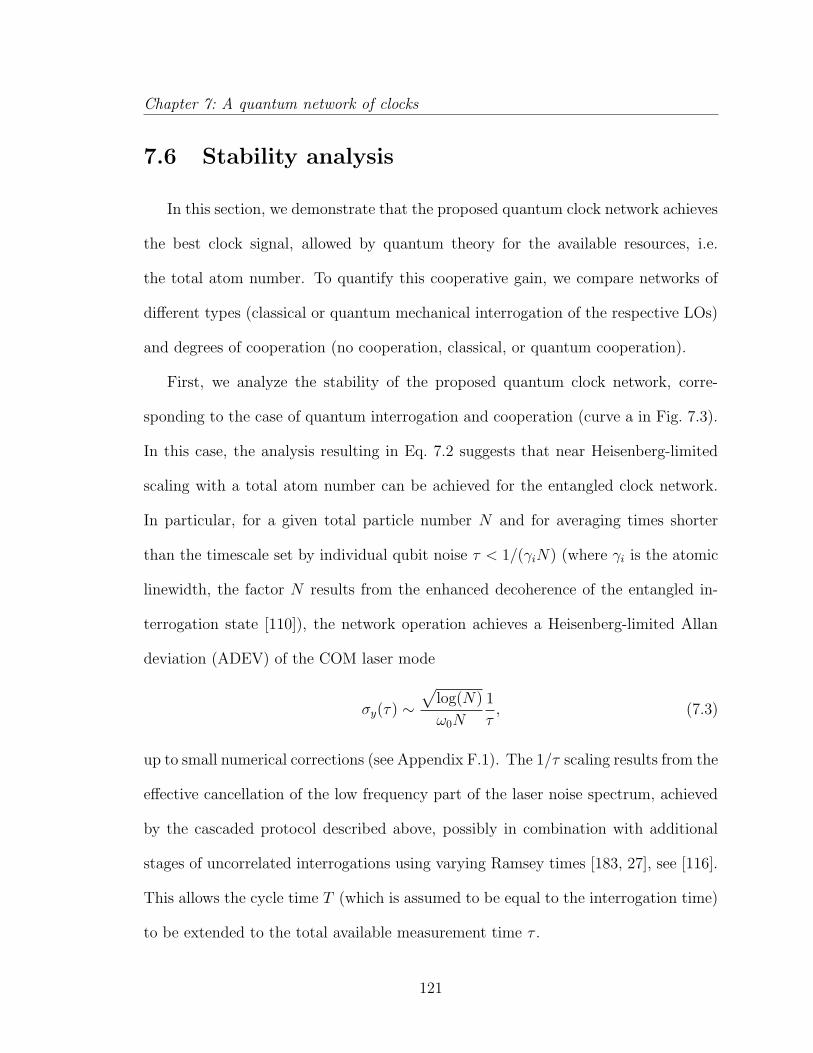
Chapter 7: A quantum network of clocks
7.6 Stability analysis
In this section, we demonstrate that the proposed quantum clock network achieves
the best clock signal, allowed by quantum theory for the available resources, i.e.
the total atom number. To quantify this cooperative gain, we compare networks of
different types (classical or quantum mechanical interrogation of the respective LOs)
and degrees of cooperation (no cooperation, classical, or quantum cooperation).
First, we analyze the stability of the proposed quantum clock network, corre-
sponding to the case of quantum interrogation and cooperation (curve a in Fig. 7.3).
In this case, the analysis resulting in Eq. 7.2 suggests that near Heisenberg-limited
scaling with a total atom number can be achieved for the entangled clock network.
In particular, for a given total particle number N and for averaging times shorter
than the timescale set by individual qubit noise τ < 1/(γiN) (where γi is the atomic
linewidth, the factor N results from the enhanced decoherence of the entangled in-
terrogation state [110]), the network operation achieves a Heisenberg-limited Allan
deviation (ADEV) of the COM laser mode
σy(τ) ∼√
log(N)
ω0N
1
τ, (7.3)
up to small numerical corrections (see Appendix F.1). The 1/τ scaling results from the
effective cancellation of the low frequency part of the laser noise spectrum, achieved
by the cascaded protocol described above, possibly in combination with additional
stages of uncorrelated interrogations using varying Ramsey times [183, 27], see [116].
This allows the cycle time T (which is assumed to be equal to the interrogation time)
to be extended to the total available measurement time τ .
121
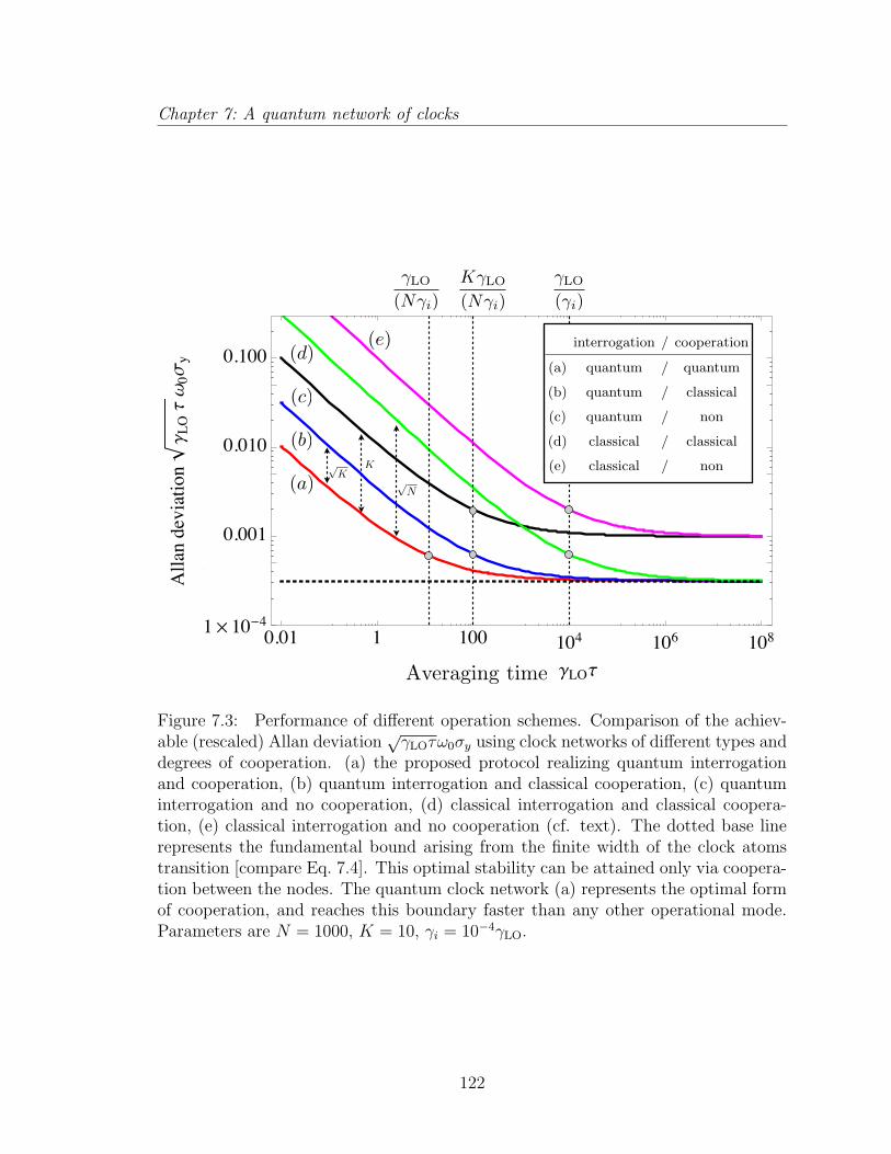
Chapter 7: A quantum network of clocks
0.01 1 100 104 106 1081¥ 10-4
5¥ 10-40.001
0.0050.010
0.0500.100
Averging time gLOt
Alla
ndeviationg L
Otw0s
y
(a)
(b)
(c)
(d)(e)
(a) – quantum/quantum
(b) – quantum/classical
(c) – quantum/non-coop
(d) – classical/classical
(e) – classical/non-coop
LO(Ni)
KLO(Ni)
LO(i)
pK
K
pN
Averaging time
2
interrogation / cooperation
(a) quantum / quantum
(b) quantum / classical
(c) quantum / non
(d) classical / classical
(e) classical / non
TABLE I: Non-exhaustive comparison of thermal phase transitions (TPT), QPT and DPT. The concepts for DPT parallel inmany respects the considerations for QPT and TPT. || · ||tr denotes the trace norm and S the entropy. Note that if the steadystate is not unique, additional steady states may come with a non-zero imaginary part of the eigenvalue and then appear inpairs: L = ±iy (y 2 R).
sults and the LO signals from the nodes in question is anindication of erroneous operation or sabotage. The secu-rity of the entire network relies on the trustworthiness ofthe center. To minimize the risk of a compromised cen-ter, the role of the center can rotate around, such thatit is always a di↵erent node that fulfills the duties of thecenter.
In what follows various elements of the proposed net-work are analyzed in details.
A. Entangling
We discuss the entangling protocol that creates aGHZ state across all clock qubits, irrespective of theirgeographic position. The qubits at the center (nodej = 0) are divided into two groups of size K, labeledby c1, c2, . . . cK and 01, 02, . . . , 0K . Qubits at node j(j = 1, 2, . . .K) are labeled as 1j , 2j , . . . nj .
The entangling procedure starts at the center with thecreation of a fully entangled state on the qubits cj.Assuming single qubit addressability, this can be real-ized with a single qubit /2-rotation around x (on c1)and a series of CNOT gates (between c1 and each cj),performed with the local oscillator field at the center,E0. The result is a GHZ state, [|00 . . . 0ic1,c2,...cK +
i|11 . . . 1ic1,c2,...cK ]/p2. In the meantime, the center
shares single EPR pairs with each node j. One leg ofthe pair is stored at the center in qubit 0j , while theother one is stored at the node in qubit 1j , forming the
states [|00i0j ,1j + |11i0j ,1j ]/p2 for every j. (See Fig. ??)
In the next step, the center performs Bell measure-ments on the cj , 0j qubit pairs. This teleports the stateof qubit cj to qubit 1j , up to a local single-qubit rotation,which is performed after the measurement outcomes aresent to the node, via classical channels. The collectiveresult of the teleportations is a GHZ state on the qubits11, 12, . . . 1K , stretching across the K nodes.
In the final step of entangling, each node extends theentanglement to all of its qubits. To do this, node jperforms a series of CNOT gates controlled on 1j andtargeting qubits 2j , 3j , . . . nj , one by one. The resulting
state is [|0i + i|1i]/p2, where |0i and |1i are product
states of all qubits ij : i = 1, 2, . . . n, j = 1, 2, . . .Kbeing in |0i or |1i, respectively.
B. Measurement
After the entangling protocol succeeds, a free evolutionof duration T takes place, during which each clock qubitat node j picks up a relative phase j = jT between |0iand |1i. These phases add up in the GHZ state to give
[|0i+ iei|1i]/p2, where the collective phase is
=KX
j=1
nj = nKCOMT, (1)
where COM =PK
j=1 j/K is the detuning of the center-
of-mass frequency, COM =PK
j=1 j/K, from !0.After the free evolution time, the qubits are measured
in order to obtain information on . Each node j mea-sures the qubits 1j , 2j , . . . nj one by one in the x-basis
|±i = (|0i± |1i)/p2, obtains qij = ±1 outcomes, and
sends them to the center via classical channels. The cen-ter evaluates the parity of all outcomes p =
Qi,j qij , and
records it as the collective outcome of the Ramsey cycle.A single instance of p holds one bit of information about, since its distribution is P(p = ±1) = [1± sin]/2.
C. Feedback
A feedback scheme is needed to create a collective clocksignal with enhanced stability. Since one Ramsey cycleprovides only a single bit p, to be conclusive about thevalue of , the cycle either has to be repeated withina short period of time or, by splitting up the resources,multiple copies have to be run in parallel. Irrespectiveof which way we choose, in the end, the center gathersenough information to estimate the true value of .In the meantime, the center generates the center-of-
mass of the frequencies. Every node sends its local oscil-lator field Ei to the center, and the center synthesizes theCOM frequency COM, by averaging the j frequencies
Figure 7.3: Performance of different operation schemes. Comparison of the achiev-able (rescaled) Allan deviation
√γLOτω0σy using clock networks of different types and
degrees of cooperation. (a) the proposed protocol realizing quantum interrogationand cooperation, (b) quantum interrogation and classical cooperation, (c) quantuminterrogation and no cooperation, (d) classical interrogation and classical coopera-tion, (e) classical interrogation and no cooperation (cf. text). The dotted base linerepresents the fundamental bound arising from the finite width of the clock atomstransition [compare Eq. 7.4]. This optimal stability can be attained only via coopera-tion between the nodes. The quantum clock network (a) represents the optimal formof cooperation, and reaches this boundary faster than any other operational mode.Parameters are N = 1000, K = 10, γi = 10−4γLO.
122
Chapter 7: A quantum network of clocks
Eventually, for large averaging times τ > 1/(γiN) the Ramsey time becomes fun-
damentally limited by individual noise processes that determine the atomic linewidth
T ≤ 1/(γiN). As a result, the 1/N scaling breaks down, and the ADEV returns to
the square root scaling with both the employed particle number and averaging time,
σy(τ) ∼ 1
ω0
√N
√γiτ, (7.4)
up to constant numerical factors. Eq. 7.4 results from fundamental quantum metro-
logical bounds [82] (In the case of dominating trap losses, the loss rate simply replaces
γi in the above formula.), and represents the best conceivable clock stability in the
presence of individual particle decoherence which, in a network, can only be achieved
via cooperation. Independently operating a clock, in contrast, can only achieve a
stability scaling with the local number of atoms, i.e. σy(τ) ∝√K/N .
Fig. 7.3 illustrates the comparison of entangled clock network with other ap-
proaches. A network in which the K nodes cooperate classically (curve b in Fig. 7.3),
by locally measuring the individual phase deviation φj, and combining the outcomes
via classical channels, outperforms individually operated clocks (curve c) by a factor
of√K (for both cases, assuming optimal quantum interrogation for individual nodes
[116, 28]). The quantum network protocol (curve a) increases this cooperative advan-
tage by an additional factor of√K for short averaging times, reaching Heisenberg-
limit, Furthermore the ADEV converges to the fundamental bound [Eq. 7.4] K times
faster compared to the case of classical cooperation (curve b). Although an optimal,
classical, local protocol (e.g. [183, 27]), combined with classical cooperation (curve
d), eventually reaches the same bound [Eq. 7.4], this approach is atom-shot noise
limited, and hence its stability is reduced by a factor of√N for short averaging times
123
Chapter 7: A quantum network of clocks
[compare Eq. 7.3] compared to the quantum network protocol. Hence, the optimal
stability [Eq. 7.4] is reached at averaging times that are N times longer than for the
proposed quantum network. Naturally, all of the above approaches are superior to a
classical scheme without cooperation (curve e).
As a specific example, we first consider ion clocks that can currently achieve a
stability of 2.8 × 10⁻¹⁵ after 1 s of averaging time [52]. The entangled states of up
to 14 ions has already been demonstrated [153] as was the entanglement of remote
ions [144]. We consider a network of ten clocks, each containing ten ions. Using Al+
(ω0 = 2π×1121 THz, γi = 2π×8 mHz), we find that the quantum cooperative protocol
can reach 4 × 10⁻¹⁷ fractional frequency uncertainty after 1 s. Larger improvements
could potentially be achieved using e.g. Yb+ ions, due to the long coherence time
(2.2× 10⁴ s) of its octupole clock transition.
The quantum gain could be even more pronounced for neutral atomic clocks. For
a network consisting of ten clocks similar to the one operated in JILA [23], each con-
taining 1000 neutral atoms with central frequency ω0 = 2π × 429 THz and linewidth
γi = 2π×1 mHz, the quantum cooperative scheme can achieve a stability of ∼ 2×10⁻¹⁸
after 1s averaging, and is an order of magnitude better than the best classical cooper-
ative scheme. Future advances, employing clock transitions with linewidths of a few
tens of µHz (such as erbium), could possibly allow for further improvement, achieving
fractional frequency uncertainty beyond 10−20 after τ ∼ 100 s. This level of stability
is in the same order of magnitude as the required sensitivity to successfully use the
network as a gravitational interferometer [197].
So far we have assumed perfect operation and infinitely fast entanglement distribu-
124

Chapter 7: A quantum network of clocks
tion rates. In Appendix F.3, we analyze these assumption and find that the advantage
of our scheme persists provided that fidelity of the local collective entangling [207]
(which creates a GHZ state of N/K qubits) exceeds the threshold fidelity Fth, where
1− Fth ∼ 1/(K logN), and the EPR sharing rate is higher than REPR ∼ (logN)2γi.
For the optical clock example presented above, Fth ∼ 0.99, and REPR ∼ 1 Hz. While
local operations with fidelity ∼ 0.95 have been realized for N ∼ 5 ions [153], the
errors in such operations increase with N , making this realization more challenging.
7.7 Security
A network with such precise time-keeping capabilities can be subject to both
internal and external attacks. Effectively countering them is crucial to establish a
reliable ground for cooperation. We consider the network secure if the implemented
countermeasures can prevent external parties from benefiting from the network (eaves-
dropping), as well as effectively detect any malicious activities of any of the members
(sabotage).
Sabotage describes the situation where one of the nodes – intended or unintended
– operates in a damaging manner. For example, one node could try sending false
LO frequencies or wrong measurement bits in the hope of corrupting the collective
measurement outcomes. In order to detect such malicious participants, the central
node can occasionally perform assessment tests of the different nodes by teleporting an
uncorrelated qubit state [|0〉+eiχ|1〉]/√
2, where χ is a randomly chosen phase known
only to the center. By checking for statistical discrepancies between the measurement
results and the detuning of the LO signal sent by the node under scrutiny, the center
125

Chapter 7: A quantum network of clocks
can rapidly and reliably determine whether the particular node is operating properly
(See Fig. 7.4a and Appendix F.2), however this strategy breaks down, if multiple
sabotage attacks happen within a short time.
Eavesdropping, i.e., the unauthorized attempt to access the stabilized νCOM fre-
quency, can be prevented by encoding the classical channels, over which the center
and the nodes exchange feedback signals, using quantum key distribution protocols
[96]. Our protocol can keep the stabilized signal hidden from outsiders by mixing the
feedback signal with the LO signal at each node only after the non-stabilized LO has
been sent to the center (see Fig. 7.4b and Appendix F.2). As a result, even if all
LO signals are intercepted, the eavesdropper is able to access only the non-stabilized
COM signal. Furthermore, the center exclusively can decode the measurement re-
sults sent by the individual nodes using its own measurement outcomes as mentioned
above. As a result, the stabilized COM signal remains accessible exclusively to parties
involved in the collaboration.
Finally, we note that a distributed operation offers significant security advantages
over an alternative approach of having all resources combined in one place from where
the signal is distributed. In case of a physical attack of the network, disabling the
center or the communication links, the nodes can fall back to an independent clock
operation using their local resources.
7.8 Outlook
One of the advantages of the proposed quantum clock network involves its ability
to maintain and synchronize the time standards across multiple parties in real-time.
126
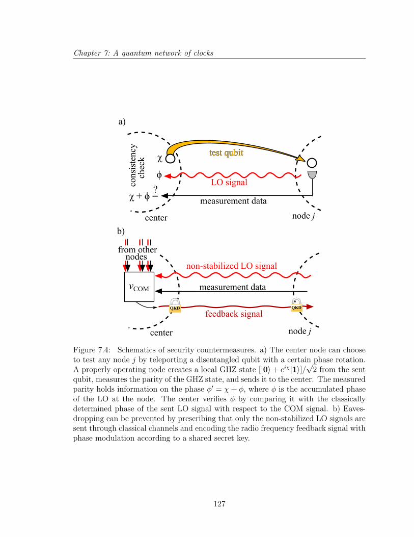
Chapter 7: A quantum network of clocks
Figure 7.4: Schematics of security countermeasures. a) The center node can chooseto test any node j by teleporting a disentangled qubit with a certain phase rotation.A properly operating node creates a local GHZ state [|0〉+ eiχ|1〉]/
√2 from the sent
qubit, measures the parity of the GHZ state, and sends it to the center. The measuredparity holds information on the phase φ′ = χ+ φ, where φ is the accumulated phaseof the LO at the node. The center verifies φ by comparing it with the classicallydetermined phase of the sent LO signal with respect to the COM signal. b) Eaves-dropping can be prevented by prescribing that only the non-stabilized LO signals aresent through classical channels and encoding the radio frequency feedback signal withphase modulation according to a shared secret key.
127
Chapter 7: A quantum network of clocks
Unlike the current world time standard, where the individual signals from different
clocks are averaged and communicated with a time delay (a so called paper clock), in
our quantum clock network, all participants have access to the ultra-stable signal at
any time. This makes it possible to measure systematic errors of different clocks in
real time, which in turn allows to correct them [23], unlike in the case of the paper
clock which has to rely on the retrospectively averaged time signals (see Appendix
F.3). The enhanced stability of the network signal hereby allows for longer Ramsey
times in the control measurements used to determine the systematics of the single
clock. Furthermore, by having full access to their local clocks the different parties
keep their full sovereignty and ensure security, as opposed to a joint operation of a
single clock.
Realization of the full-scale network of the type described here will require a num-
ber of technological advances in both metrology and experimental quantum informa-
tion science. The remote entanglement can be implemented by using recently demon-
strated techniques for individual atom-photon entanglement [163, 53, 221, 20, 180].
Since the teleportation protocol requires quantum links capable of sharing EPR pairs
with sufficiently high repetition rate and fidelity, entanglement purification [76] and
quantum repeater techniques [70] will likely be required. In practice, qubits used for
entanglement distribution may not be ideal for clocks. However, as noted previously
remote entanglement does not need to involve coherent qubits at optical frequencies
(e.g., polarization entanglement can be used). In such a case, the use of hybrid ap-
proaches, combining different systems for entanglement and local clock operations,
may be warranted. Similarly, signals from clocks employing different transition fre-
128
Chapter 7: A quantum network of clocks
quencies can be coherently connected by frequency combs, allowing clocks with differ-
ent clock qubits to participate. It might also be interesting to explore if high-fidelity
entangled EPR pairs can be used to create remote entangled states of spin-squeezed
type [127, 202, 136], or by following the proposed approach for cat state preparation
in atomic ensembles [146], or using collective interactions (such as [207]) and repeti-
tive teleportation [5]. In addition, while space-based communication networks will be
capable of maintaining optical phase coherence for the links between clocks, we note
that establishing ground-space coherent optical links remains a technical challenge
and requires an intense research effort which has recently started [64]. Finally, if the
entire network is spanned by satellites in space, the on-board local oscillators can
further benefit from the much lower noise level compared to ground-based clocks.
If realized, such a quantum network of clocks can have important scientific, tech-
nological, and social consequences. Besides creating a world platform for time and
frequency metrology, such a network may find important applications to a range of
technological advances for earth science [214], precise navigation of autonomous vehi-
cles and space probes (requiring high refresh rate), and to the test and search for the
fundamental laws of nature, including relativity and the connection between quan-
tum and gravitational physics [1, 201, 197, 238]. In order to explore these exciting
applications one can either use the excellent common frequency reference generated
by the clock network, or, alternatively, prepare modified collective states of different
nodes that can directly measure the specific signal under study.
129

Chapter 8
Quantum network of neutral atom
clocks
8.1 Introduction
The current record in clock precision is held by ytterbium and strontium clocks
[131], capable of reaching ∼ 10−18 total fractional frequency uncertainty. Apart from
the enormous amount of effort and innovation, this unprecedented accuracy was at-
tainable due to the large number of clock atoms (103 − 104) [107, 23, 157]. In our
recent work [121], we showed that a quantum network of atomic clocks can result in
substantial boost of the overall accuracy if multiple clocks are connected in quantum
entanglement. The proposed globally entangled state, Greenberger-Horne-Zeilinger
(GHZ) state, is more sensitive to the global phase evolution of the clock atoms, and
allows for an improved measurement of the passage of time. If the GHZ state is
set up and interrogated in the optimal way [116, 21], frequency measurements can
130
Chapter 8: Quantum network of neutral atom clocks
asymptotically reach the Heisenberg limit [102], associated with the total number of
atoms in the entire network.
Imperfections during creation of the GHZ state are the main obstacles for experi-
mental realizations of a quantum clock network. Errors arising during the distribution
of entanglement add up, and limit the total number of atoms and clocks with which
the fidelity does not drop significantly. Efforts are being made to make both the non-
local [192] and local entanglement distribution [206, 190] faster and more reliable. Of
particular interest are applications of these ideas to neutral atom clocks.
In this Letter, we show how a non-local GHZ state can be created across multi-
ple, spatially separated neutral atom clocks with high fidelity. Our protocol relies on
strong Rydberg blockade for enhancing local atom-atom interaction, collective exci-
tations for enhancing photon-atom interaction, and single photon quantum channels
at telecom frequency for reliable non-local connections. We propose and analyze a
realization using neutral Yb ensembles, suitable for the current atomic clock technol-
ogy.
Rydberg blockade is a result of the interaction arising between atoms excited to
Rydberg states in an ensemble. If driven resonantly, the first excited atom blocks
the transition of a second one, thus at most one atom can get coherently excited to
the Rydberg state [73, 74, 77], allowing precise quantum control. Rydberg blockade
has been proposed as an efficient tool to realize quantum gates and perform quantum
information processing [135, 154, 190, 244, 104, 97]. Different ways of trapping and
manipulating Rydberg states are currently under investigation both experimentally
[46, 12, 87, 8, 232] and theoretically [223, 22, 224].
131
Chapter 8: Quantum network of neutral atom clocks
8.2 Description of the protocol
We describe our protocol for K identical atomic clocks arranged in a sequence, each
connected to its neighbors with optical channels, and each using n identical atoms,
trapped in an optical lattice. We use the atomic levels, shown on Fig. 8.1(a) for
our protocol: The two levels of the clock transition, g, f , a metastable shelving level
s, an excited level e, which spontaneously decays to g, and two strongly interacting
Rydberg levels, r1 and r2. We further require transitions between levels, marked with
arrows, to be driven independently.
We imagine preparing all atoms in the ground state g, after which our protocol
consists of five subsequent steps. First, using blockade, we create two independent
collective excitations in each ensemble, using two separate atomic levels (f and s).
Second, each ensemble emits single photon pulses that are entangled with one of
these collective excitations. Third, the photons are sent towards the neighboring
atomic clocks, and measured with a linear optics setup in Bell-basis. Fourth, upon
success, each clock performs a local CNOT operation to connect the two collective
excitations. The result is a set of K entangled collective excitations, one in each
clock, which serve as ”seeds” for a global GHZ state. In the fifth, and final, step the
clocks locally ”grow” a GHZ state out of each seed, and thus a global GHZ state is
obtained. In the following, we provide detailed description and analysis of these five
steps, discuss the specific realization in Yb atoms and analyze the most important
sources of imperfections and errors.
132
Chapter 8: Quantum network of neutral atom clocks
8.2.1 Collective excitations
In the first step, we make use of the Rydberg blockade to create a superposition of
one and zero excitation in both f and s levels, following the approach of [135, 190, 73].
This is done by performing the following sequence of driving pulses: [π/(2√n)]g,r1,
[π]f,r1, [π]f,s, [(π/(2√n)]g,r1, [π]f,r1, shown on Fig. 8.1(a), where [φ]a,b stands for a
pulse with total, single-atom Rabi phase φ between level a and b. Starting from the
state |g〉⊗n =: |0〉, this pulse sequence creates the state
(1 + f †)(1 + s†)|0〉 =:(|0f〉+ |1f〉
)(|0s〉+ |1s〉
), (8.1)
where f † and s† are creation operators of the two (approximately) independent spin
wave modes, supported by the two levels f and s.
8.2.2 Non-local connection
In the second step, spin-photon entangled states, using the spin wave modes f and
s, are created, using the an extended version of the scheme described in [128]. Each
spin-photon entangled state is created by the pulse sequence shown on Fig. 8.1(b),
involving [π]s,r2, [π/√n]g,r1, [π]e,r1, [π]s,r2. With additional pulses applied before and
after this sequence flipping the states of f and s waves, and proper timing, this
is repeated four times to produce four time-bin separated light pulses, which are
entangled with the two spin waves,
(|0f〉|t2〉+ |1f〉|t4〉
)(|0s〉|t1〉+ |1s〉|t3〉
)(8.2)
where |tj〉|tk〉 is a two-photon state with photons emitted at times tj and tk.
133
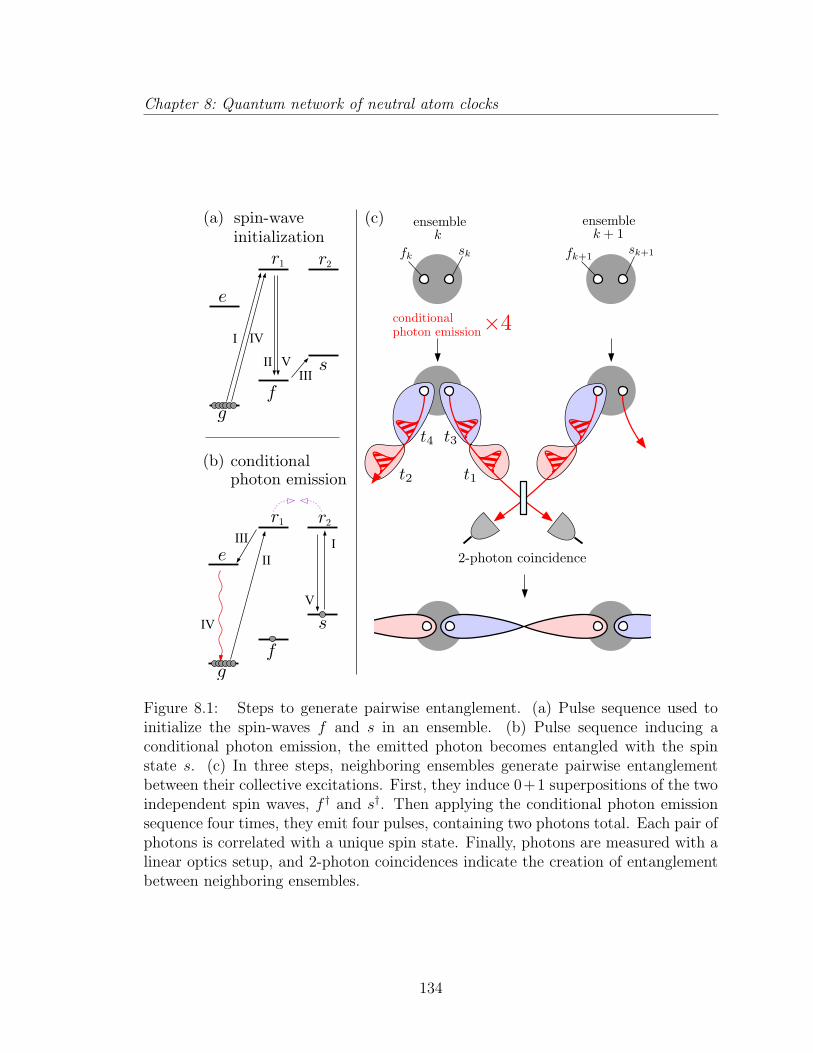
Chapter 8: Quantum network of neutral atom clocks
Figure 8.1: Steps to generate pairwise entanglement. (a) Pulse sequence used toinitialize the spin-waves f and s in an ensemble. (b) Pulse sequence inducing aconditional photon emission, the emitted photon becomes entangled with the spinstate s. (c) In three steps, neighboring ensembles generate pairwise entanglementbetween their collective excitations. First, they induce 0+1 superpositions of the twoindependent spin waves, f † and s†. Then applying the conditional photon emissionsequence four times, they emit four pulses, containing two photons total. Each pair ofphotons is correlated with a unique spin state. Finally, photons are measured with alinear optics setup, and 2-photon coincidences indicate the creation of entanglementbetween neighboring ensembles.
134
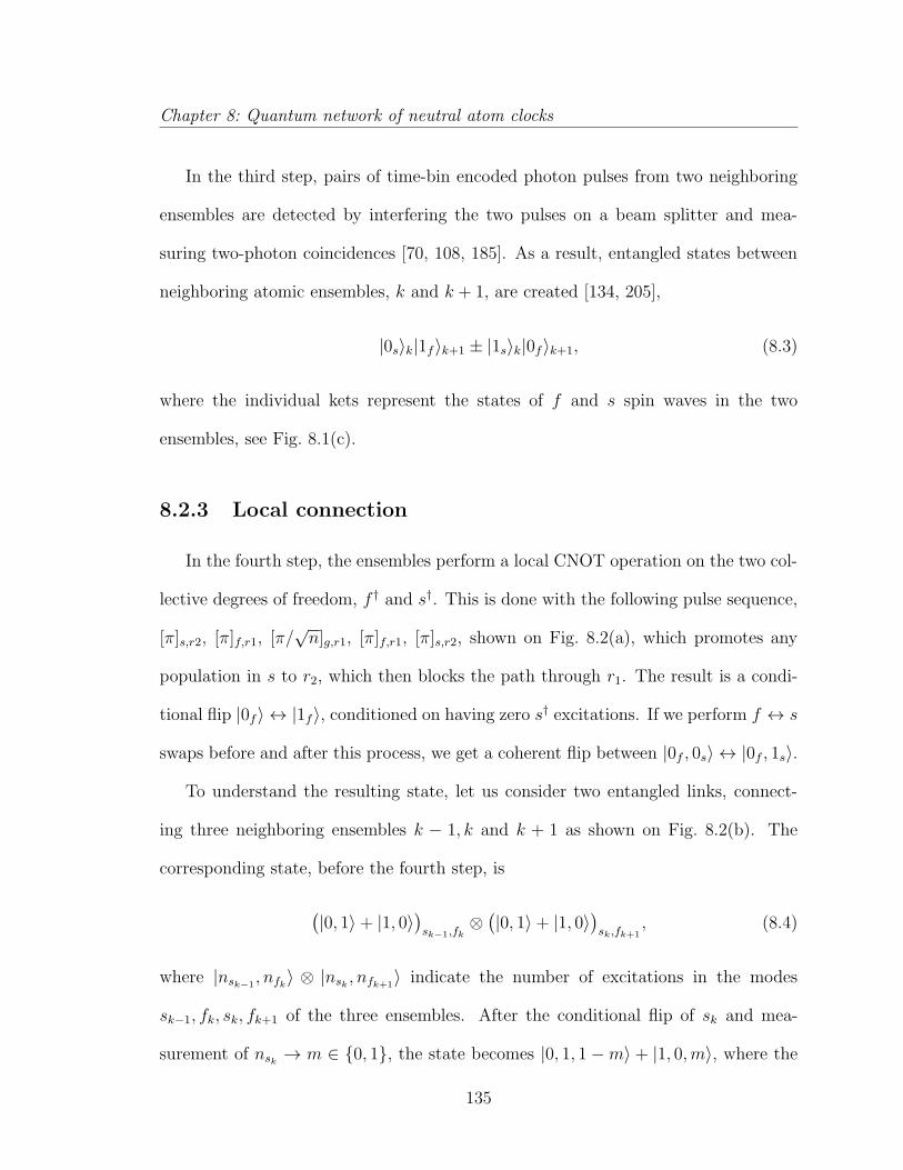
Chapter 8: Quantum network of neutral atom clocks
In the third step, pairs of time-bin encoded photon pulses from two neighboring
ensembles are detected by interfering the two pulses on a beam splitter and mea-
suring two-photon coincidences [70, 108, 185]. As a result, entangled states between
neighboring atomic ensembles, k and k + 1, are created [134, 205],
|0s〉k|1f〉k+1 ± |1s〉k|0f〉k+1, (8.3)
where the individual kets represent the states of f and s spin waves in the two
ensembles, see Fig. 8.1(c).
8.2.3 Local connection
In the fourth step, the ensembles perform a local CNOT operation on the two col-
lective degrees of freedom, f † and s†. This is done with the following pulse sequence,
[π]s,r2, [π]f,r1, [π/√n]g,r1, [π]f,r1, [π]s,r2, shown on Fig. 8.2(a), which promotes any
population in s to r2, which then blocks the path through r1. The result is a condi-
tional flip |0f〉 ↔ |1f〉, conditioned on having zero s† excitations. If we perform f ↔ s
swaps before and after this process, we get a coherent flip between |0f , 0s〉 ↔ |0f , 1s〉.
To understand the resulting state, let us consider two entangled links, connect-
ing three neighboring ensembles k − 1, k and k + 1 as shown on Fig. 8.2(b). The
corresponding state, before the fourth step, is
(|0, 1〉+ |1, 0〉
)sk−1,fk
⊗(|0, 1〉+ |1, 0〉
)sk,fk+1
, (8.4)
where |nsk−1, nfk〉 ⊗ |nsk , nfk+1
〉 indicate the number of excitations in the modes
sk−1, fk, sk, fk+1 of the three ensembles. After the conditional flip of sk and mea-
surement of nsk → m ∈ 0, 1, the state becomes |0, 1, 1 −m〉 + |1, 0,m〉, where the
135
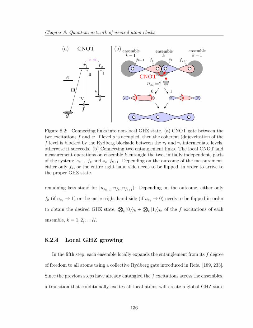
Chapter 8: Quantum network of neutral atom clocks
Figure 8.2: Connecting links into non-local GHZ state. (a) CNOT gate between thetwo excitations f and s: If level s is occupied, then the coherent (de)excitation of thef level is blocked by the Rydberg blockade between the r1 and r2 intermediate levels,otherwise it succeeds. (b) Connecting two entanglement links. The local CNOT andmeasurement operations on ensemble k entangle the two, initially independent, partsof the system: sk−1, fk and sk, fk+1. Depending on the outcome of the measurement,either only fk, or the entire right hand side needs to be flipped, in order to arrive tothe proper GHZ state.
remaining kets stand for |nsk−1, nfk , nfk+1
〉. Depending on the outcome, either only
fk (if nsk → 1) or the entire right hand side (if nsk → 0) needs to be flipped in order
to obtain the desired GHZ state,⊗
k |0f〉k +⊗
k |1f〉k, of the f excitations of each
ensemble, k = 1, 2, . . . K.
8.2.4 Local GHZ growing
In the fifth step, each ensemble locally expands the entanglement from its f degree
of freedom to all atoms using a collective Rydberg gate introduced in Refs. [189, 233].
Since the previous steps have already entangled the f excitations across the ensembles,
a transition that conditionally excites all local atoms will create a global GHZ state
136

Chapter 8: Quantum network of neutral atom clocks
Figure 8.3: Local GHZ creation. (a) Conditional, local GHZ state generation: Anyexcitation in level s prevents the dressing of g with r1, which, otherwise introducesa π phase shift on g. With the conjugation of π/2 pulses II and VI, this results ina transfer from g to f conditioned on the population of s. (b) The local entanglingoperation extends the GHZ state from the f spin-wave to all atoms. As a result,every atom in the network gets entangled.
of every atom in the network. The pulse sequence [π]f,s, [π/2]g,f , [π]s,r2, [π(∆)]g,r1,
[π]s,r2, [π/2]g,f , shown in Fig. 8.3(a), does exactly that, where [π(∆)]g,r1 is an off-
resonant dressing pulse, whose Rabi frequency Ω and duration is set properly in
order to introduce a conditional π phase shift on level g. This sequence transfers the
atoms from g to f only if r2 is unoccupied, and gets blocked otherwise. The result is
K⊗
k=1
|0f〉k +K⊗
k=1
|1f〉k →K⊗
k=1
|f〉⊗n +K⊗
k=1
s†|g〉⊗n, (8.5)
where |f〉 and |g〉 denote the state of a single atom. Finally, we get rid of the s
excitation with a series of pulses that move it back to g: [π]f,s, [π]f,r1, [π]f,s, [π/√n]g,r1,
and end up with |f〉⊗Kn + |g〉⊗Kn, a fully entangled state of all N = Kn atoms in the
network.
137
Chapter 8: Quantum network of neutral atom clocks
8.3 Implementation
We next investigate the robustness of our protocol in light of realistic physical
imperfections. We assume that all imperfections decrease the coherence between
the two components of the GHZ state, and therefore the fidelity can be written as
F = [1 + exp(−εtot)]/2, where εtot is the sum of the errors. The errors arising during
each non-local connection step εnon−local and the errors arising during a local GHZ
creation in one clock εlocal add up to the total error εtot = (K − 1)εnon−local +Kεlocal,
and overall fidelity
F ≥
1 + exp[−N
(εnon−local
n+εlocal
n
)]/2. (8.6)
The error, εtot, increases linearly with the total number of atoms in the network, N ,
and the coefficient, (εnon−local + εlocal)/n, depends on the number of atoms, n, at a
single site. For a certain optimal local atom number nopt, the total fidelity is maximal,
i.e. decreases with the slowest rate, as N increases. Evenly distributing the atoms
into Kopt = N/nopt groups is therefore optimal.
To be specific, we focus on a possible implementation of our scheme with en-
sembles of neutral ytterbium atoms whose relevant electronic levels are shown on
Fig. 8.4. We identify the following levels of neutral Yb relevant for our protocol:
|g〉 = |6s6p(3P0)〉, |f〉 = |6s2(1S0)〉, |s〉 = |6s6p(3P2)〉 and |e〉 = |5d6s(3D1)〉, and two
Rydberg levels |r1〉 = |6sns(1S0)〉 and |r2〉 = |6snpm=+1(1P1)〉 with the same principle
quantum number n. Although the branching ratio for the e → g decay is not unity,
the large population in g collectively enhances this decay channel, and the transition
becomes effectively closed. Due to the different symmetries of these states, the co-
138
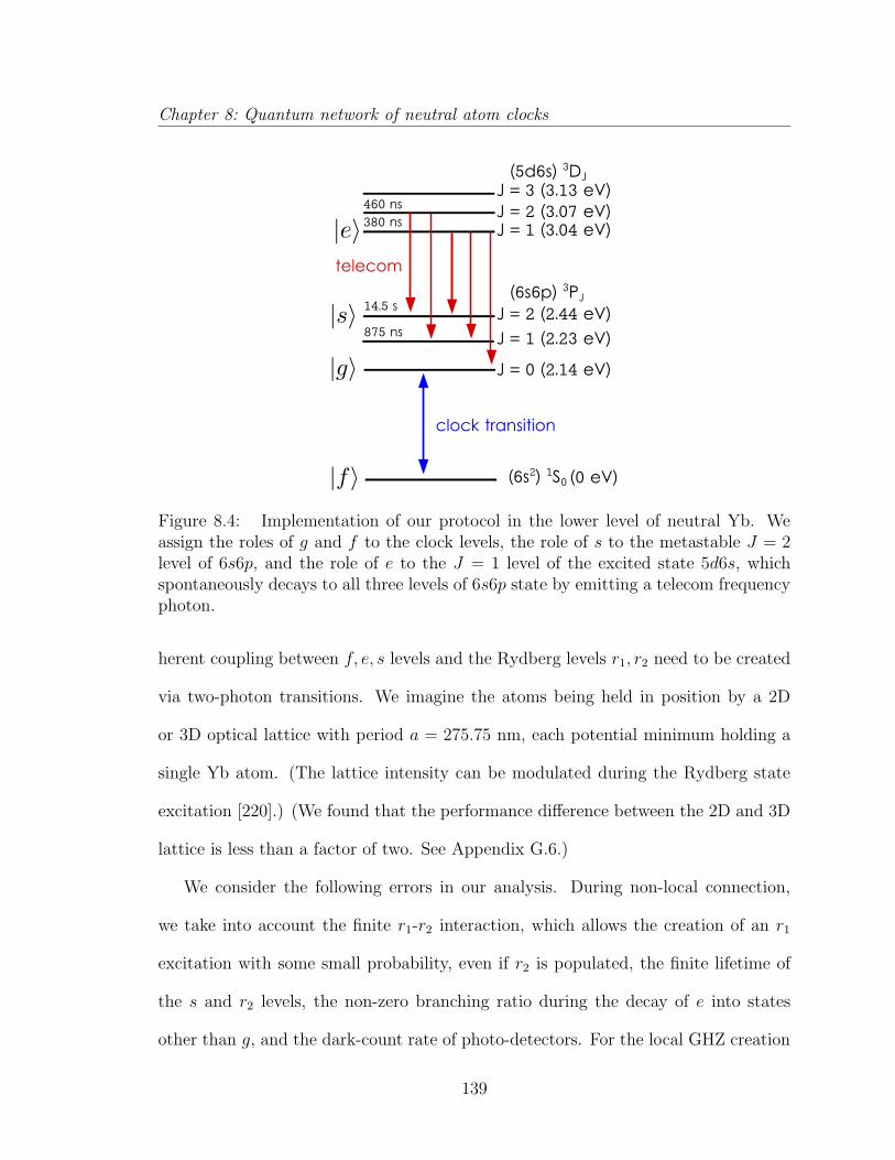
Chapter 8: Quantum network of neutral atom clocks
Figure 8.4: Implementation of our protocol in the lower level of neutral Yb. Weassign the roles of g and f to the clock levels, the role of s to the metastable J = 2level of 6s6p, and the role of e to the J = 1 level of the excited state 5d6s, whichspontaneously decays to all three levels of 6s6p state by emitting a telecom frequencyphoton.
herent coupling between f, e, s levels and the Rydberg levels r1, r2 need to be created
via two-photon transitions. We imagine the atoms being held in position by a 2D
or 3D optical lattice with period a = 275.75 nm, each potential minimum holding a
single Yb atom. (The lattice intensity can be modulated during the Rydberg state
excitation [220].) (We found that the performance difference between the 2D and 3D
lattice is less than a factor of two. See Appendix G.6.)
We consider the following errors in our analysis. During non-local connection,
we take into account the finite r1-r2 interaction, which allows the creation of an r1
excitation with some small probability, even if r2 is populated, the finite lifetime of
the s and r2 levels, the non-zero branching ratio during the decay of e into states
other than g, and the dark-count rate of photo-detectors. For the local GHZ creation
139
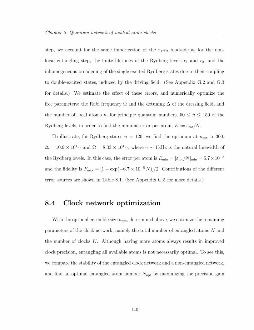
Chapter 8: Quantum network of neutral atom clocks
step, we account for the same imperfection of the r1-r2 blockade as for the non-
local entangling step, the finite lifetimes of the Rydberg levels r1 and r2, and the
inhomogeneous broadening of the single excited Rydberg states due to their coupling
to double-excited states, induced by the driving field. (See Appendix G.2 and G.3
for details.) We estimate the effect of these errors, and numerically optimize the
free parameters: the Rabi frequency Ω and the detuning ∆ of the dressing field, and
the number of local atoms n, for principle quantum numbers, 50 ≤ n ≤ 150 of the
Rydberg levels, in order to find the minimal error per atom, E := εtot/N .
To illustrate, for Rydberg states n = 120, we find the optimum at nopt ≈ 300,
∆ = 10.9 × 10⁴ γ and Ω = 8.33 × 10⁴ γ, where γ ∼ 1 kHz is the natural linewidth of
the Rydberg levels. In this case, the error per atom is Emin = [εtot/N ]min = 6.7×10⁻⁵
and the fidelity is Fmax = [1 + exp(−6.7× 10⁻⁵ N)]/2. Contributions of the different
error sources are shown in Table 8.1. (See Appendix G.5 for more details.)
8.4 Clock network optimization
With the optimal ensemble size nopt, determined above, we optimize the remaining
parameters of the clock network, namely the total number of entangled atoms N and
the number of clocks K. Although having more atoms always results in improved
clock precision, entangling all available atoms is not necessarily optimal. To see this,
we compare the stability of the entangled clock network and a non-entangled network,
and find an optimal entangled atom number Nopt by maximizing the precision gain
140
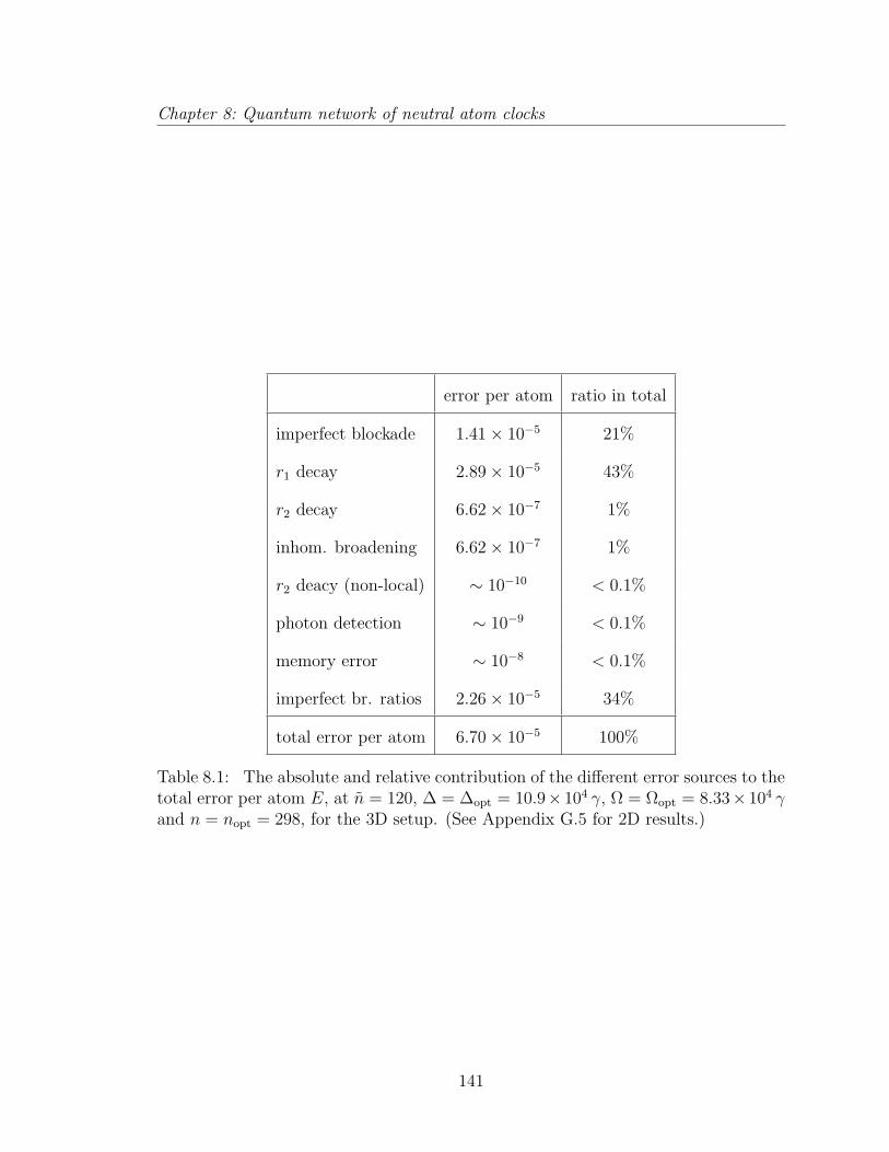
Chapter 8: Quantum network of neutral atom clocks
error per atom ratio in total
imperfect blockade 1.41× 10⁻⁵ 21%
r1 decay 2.89× 10⁻⁵ 43%
r2 decay 6.62× 10⁻⁷ 1%
inhom. broadening 6.62× 10⁻⁷ 1%
r2 deacy (non-local) ∼ 10−10 < 0.1%
photon detection ∼ 10−9 < 0.1%
memory error ∼ 10−8 < 0.1%
imperfect br. ratios 2.26× 10⁻⁵ 34%
total error per atom 6.70× 10⁻⁵ 100%
Table 8.1: The absolute and relative contribution of the different error sources to thetotal error per atom E, at n = 120, ∆ = ∆opt = 10.9× 10⁴ γ, Ω = Ωopt = 8.33× 10⁴ γand n = nopt = 298, for the 3D setup. (See Appendix G.5 for 2D results.)
141
Chapter 8: Quantum network of neutral atom clocks
over the non-entangled scheme,
G =σnon−ent
σent/(2F − 1)= e−EN
π
8
√N
logN, (8.7)
where σent = 1ω0τ
8π
√logNN
(from [121], assuming perfect fidelity, and that τ is smaller
than the reduced atomic coherence time γ−1at /N) and σnon−ent = 1
ω0τ1√N
(for N in-
dependent atoms) are the Allan-deviations of the two schemes, where ω0 is the cen-
tral frequency and τ is the total available measurement time. The additional factor
of 2F − 1 = e−EN is due to the reduced Fisher information of a non-pure GHZ
state, where E is the error per atom and F is the fidelity of the initial state. (See
Appendix G.6 for details.) For E = Emin = 6.7 × 10⁻⁵, Eq. 8.7 is maximal at
Nopt ≈ 1/(2Emin) ≈ 7500, where Gmax = 6.9, and F = [1 + e−NoptEmin ]/2 = 0.82.
The above optimum is achieved by 7500 atoms distributed in Kopt = Nopt/nopt ≈
22 clocks. Since current lattice clocks can employ 103−104 atoms, we can imagine en-
tangling this many atoms in a single vacuum chamber. With realistic atom densities,
the atoms need to be separated into ∼ 102 ensembles, for efficient Rydberg blockade.
We imagine using an individually addressed “messenger” atom, that can be moved to
the vicinity of each ensemble, and can be brought to entanglement with them using
dipole-dipole interaction. (See Appendix G.7 for more details.) Such a scheme is free
from imperfections affecting the photons in the previous scheme, and thus can reach
a higher fidelity for a given number of atoms, or use more atoms to achieve a higher
gain. We find that, at the optimum, the gain over the classical scheme is ∼ 14, twice
the gain of the network scheme.
142
Chapter 8: Quantum network of neutral atom clocks
8.5 Conclusion
We presented and analyzed a protocol, capable of fully entangling ensembles of
neutral atoms located in different atomic clocks. Local interactions are made robust
by utilizing the strong interaction between Rydberg excitations, and non-local entan-
glement creation is made reliable with strong atom-light coupling, suppressed photon
propagation errors and long atomic memory lifetimes. We showed that our scheme,
in particular a realization with neutral Yb ensembles, is feasible and provides signifi-
cant gain over non-entangled schemes even in the light of physical imperfections. Our
results provide the first detailed proposal for a network that can serve as a prototype
of the global quantum clock network outlined in [121].
143
Appendix A
Appendices for Chapter 2
A.1 Derivation of reflected mode operator
We obtain the reflected mode operator cR using input-output relations for a two-
sided cavity. By assuming that the two endmirrors have the same transmittivity
(∝ κ), we can write the input-output relation for cavity mode ca on the driven mirror
as
ca,out =√κca − ca,in, (A.1)
where ca,in = −i Ω√κ
is the incoming field operator on the mirror and ca,out is the
output field operator. For direct comparision with ca we divide by√κ and define the
reflection mode operator as cR ≡ ca,out/√κ = ca + iΩ
κ.
144
Appendix A: Appendices for Chapter 2
A.2 Analytic model
In this appendix we provide the analytic solutions used to calculate one- and two-
time correlation functions in steady state. First, one-time correlations are calculated
from the steady state solutions of Eqs. (2.13–2.18). We set the time derivatives to zero
and solve the equations iteratively, order by order in the weak drive. This procedure
yields
A000 ≈ 1, (A.2)
A100 = −iα 1
1 + 4x2, (A.3)
A011 = −α 2x
1 + 4x2, (A.4)
A200 = − α2
√2
1 + 2x2
(1 + 4x2)(1 + 6x2), (A.5)
A111 = iα2 2x
(1 + 4x2)(1 + 6x2), (A.6)
A022 = α2 4x2
(1 + 4x2)(1 + 6x2), (A.7)
where α = Ω/κ (|α|2 1), x = g/(4κ) and κ = κ− i∆. Using these amplitudes, we
can express all equal time averages. The mean photon numbers are
na = |A100|2, (A.8)
ns = |A011|2, (A.9)
nR =
∣∣∣∣A100 + iΩ
κ
∣∣∣∣2
, (A.10)
145

Appendix A: Appendices for Chapter 2
and the photon-photon correlation functions are
g(2)aa (0) =
2|A200|2|A100|4
, (A.11)
g(2)ss (0) =
2|A022|2|A011|4
, (A.12)
g(2)RR(0) =
∣∣∣−(
Ωκ
)2+ 2iΩ
κA100 +
√2A200
∣∣∣2
∣∣iΩκ
+ A100
∣∣4 . (A.13)
To leading order in κ/g these yield Eqs. (2.19–2.24).
At finite temperature we calculate steady state amplitudes within each phonon
subspace n similarly in the ansatz of Eq. 2.26. Using the notation Rκ(ω) introduced
in Section 2.3.2, the steady state amplitudes within the subspace with n phonons in
the optical groundstate are
|A10n|2 =Ω2√Rκ(0)
Rκ
(g2
√n+ 1
) , (A.14)
|A01n+1|2 =Ω2g2(n+ 1)
4Rκ
(g2
√n+ 1
) , (A.15)
|A20n|2 =Ω4Rκ(g/
√8)
Rκ
(g√
(2n+ 1)/8)Rκ
(g2
√n+ 1
) , (A.16)
|A02n+2|2 =Ω4g4(n+ 1)(n+ 2)
32Rκ
(g√
(2n+ 1)/8)Rκ
(g2
√n+ 1
) . (A.17)
Two-time correlation functions are calculated similarly, using the conditional state
after a jump (see Eqs. (2.39) and (2.44)) as the initial condition. For example the
unnormalized state after detection of a photon in the ca mode is ca|ψ〉 = A100|000〉+√
2A200|100〉+A111|011〉. We solve Eqs. (2.13–2.15) for the amplitudes with this state
as initial condition. The finite delay correlation of the driven mode is
g(2)aa (τ) =
|A100(τ)|2|A100|4
. (A.18)
146
Appendix A: Appendices for Chapter 2
in good agreement with the numerics. The correlation of the undriven mode g(2)ss (τ)
is calculated similarly. The unnormalized state after detection in the cs mode is
cs|ψ〉 = A011|001〉 + A111|101〉 +√
2A022|012〉. Using this as the initial condition we
solve Eqs. (2.41–2.43) for the amplitudes in the conditional state. In the limit of
γ κ we obtain
g(2)ss (τ) =
|A012(τ)|2|A011|4
. (A.19)
147
Appendix B
Appendices for Chapter 3
B.1 Phonon nonlinearities
In Eq. (8) in the main text we have derived an effective master equation (ME)
to describe the nonlinear interaction between two phonon modes. In the following
we present an alternative, more rigorous, approach, which illustrates the individual
approximations made in the derivation of the effective phonon nonlinearity in more
detail. We first consider only a single mechanical mode, e.g. b ≡ b1, which also allows
us more easily to compare the results with exact numerical calculations of the full
model.
B.1.1 Model
We start with the full ME for the two optical modes coupled to a single resonator
mode, which in the frame of the driving frequency ωL can be written as
ρ = −i[H0 +Hg +HΩ(t), ρ] + Ldissρ. (B.1)
148
Appendix B: Appendices for Chapter 3
Here
H0 = ωmb†b−∆sc
†scs −∆ac
†aca, (B.2)
and
Hg =g0
2
(cac†sb† + c†acsb
), (B.3)
are the free evolution and the OM coupling, respectively, HΩ(t) = iΩs(t)(c†s − cs) is
the driving field for the symmetric mode with slowly varying amplitude Ωs(t) and
Ldissρ =∑
η=s,a
κD[cη]ρ+γ
2Dth[b]ρ, (B.4)
accounts for dissipation. Here we have defined the superoperator Dth[b] = (Nth +
1)D[b] +NthD[b†] to describe the coupling to a thermal bath.
B.1.2 Displaced frame
In contrast to the approach outlined in the main text, we now start our analysis
with a unitary displacement U(t)csU†(t) = cs + α(t) where the classical cavity field
α(t) obeys
α(t) = (i∆s − κ)α(t) + Ωs(t). (B.5)
This unitary transformation eliminates the classical driving field and in the new
frame the resulting ME can be written as
ρ =− i[Hlin +Hg, ρ] + Ldissρ, (B.6)
where HΩ(t) has disappeared, but the linear part of the Hamiltonian now contains
an additional coupling between the resonator and the anti-symmetric cavity mode,
Hlin = H0 +G(t)cab† +G∗(t)c†ab, (B.7)
149
Appendix B: Appendices for Chapter 3
where G(t) = g0α(t)/2. Note that ME (B.6) is still exact and we will use this equation
for our exact numerics below.
B.1.3 Hybridized modes
To proceed, we assume that α(t) is constant or slowly varying on the timescale set
by the detunings |∆a + ωim|. This allows us to write Hlin in its adiabatic eigenbasis
Hlin = −∆sc†scs − ∆aC
†C + ωmB†B, (B.8)
where the C and B are bosonic operators for the hybridized mechanical and optical
modes and ∆a and ωm are the new eigenfrequencies of Hlin for a given G ≡ G(t). We
obtain
C = cos(θ)ca − sin(θ)b, (B.9)
B = cos(θ)b+ sin(θ)ca, (B.10)
where tan(2θ) = −2|G|/δ and δ = −(∆a + ωm) = 2J − ωm − ∆s. The shifted
frequencies are given by
−∆a = −∆a −1
2
(δ −
√δ2 + 4|G|2
), (B.11)
ωm = ωm −1
2
(δ +
√δ2 + 4|G|2
). (B.12)
We see that by slowly increasing the classical control field α(t), the mechanical mode
b is adiabatically converted into a polaronic mode B. For small mixing angles θ the
mode still retains its mechanical character, while the finite photonic component is
responsible for inducing an effective nonlinearity.
150
Appendix B: Appendices for Chapter 3
In terms of the hybridized mode operators the dissipative terms can be written as
Ldiss 'κD[cs] + κ cos2(θ)D[C] +γ
2sin2(θ)Dth[C]
+γ
2cos2(θ)Dth[B] + κ sin2(θ)D[B].
(B.13)
In particular, we identify an additional optical decay channel with rate γ′ = 2κ sin2(θ)
for the B mode. In the following we define as
Lγ =γ
2cos2(θ)Dth[B] +
γ′
2D[B], (B.14)
the modified mechanical dissipation Liouvillian. Note that in Eq. (B.13) we have
already neglected cross-terms between C and B†. This is valid in the parameter
regime considered below, where κ is small compared to the splitting of these two
modes.
Finally, we also express the nonlinear interaction Hg in terms of the hybridized
modes and write the result as
Hg = H(1)g +H(2)
g +H ′g. (B.15)
Here, the first term is the one of interest
H(1)g =
g0
4sin(2θ)
(cs + c†s
)B†B, (B.16)
and describes the coupling of the cs mode to the number operator of the B mode.
The second term is given by
H(2)g = −g0
2sin2(θ)
(Bc†sC
† +B†csC), (B.17)
and leads to additional corrections. However, for small θ this term is small compared
to H(1)g . It can be further reduced if |∆s − δ| ∆s. Finally, the last term contains
151
Appendix B: Appendices for Chapter 3
interactions
H ′g =g0
2cos2(θ)
(Cc†sB
† + C†csB)− g0
4sin(2θ)
(cs + c†s
)C†C, (B.18)
which can be neglected when either the cs or the C mode are in the vacuum state.
B.1.4 Adiabatic elimination of the cavity mode
Our goal is now to derive an effective ME for the mechanical degrees of freedom
only. To do so, we write the full ME as
ρ = (L0 + L1) ρ, (B.19)
where
L0ρ = −i[Hlin +H ′g, ρ] + Ldissρ, (B.20)
and
L1ρ = −i[H(1)g +H(2)
g , ρ]. (B.21)
The dynamics of L0 does not excite the cavity modes, and therefore, in the limit
where g = g0 sin(2θ)/4 → 0 (either g0 is small or the mixing angle θ is small) the
density operator can to a good approximation be written as ρ(t) = ρm(t)⊗ ρ0c , where
ρ0c is the vacuum state of the cs and the C mode. To account for the effects of a small
L1 ∼ g up to second order in perturbation theory we define a projection operator
onto this subspace,
Pρ = Trcρ ⊗ ρ0c , (B.22)
and its complement Q = 1− P . Then
P ρ = PL0Pρ+ PL1Qρ, (B.23)
Qρ = Q(L0 + L1)Qρ+QL1Pρ. (B.24)
152
Appendix B: Appendices for Chapter 3
Up to second order in g we can formally integrate the equation for Qρ and obtain
P ρ(t) ' PL0Pρ(t) + PL1
∫ ∞
0
dτ QeL0τQL1Pρ(t). (B.25)
We define by ρm(t) = TrcPρ(t) the reduced density operator of the mechanical
mode and write the final result as
ρm(t) =(L(0)m + L(1)
m + L(2)m
)ρm(t). (B.26)
The first term describes the linear part of the dynamics
L(0)m ρm = −i[ωmB†B, ρm] + Lγρm, (B.27)
with a modified frequency and modified decay rates for the B mode. The other two
terms are given by
L(1)m ρm = −
∫ ∞
0
dτ Trc[H(1)g , eL0τ
([H(1)
g , ρm ⊗ ρ0c ])], (B.28)
and
L(2)m ρm = −
∫ ∞
0
dτ Trc[H(2)g , eL0τ
([H(2)
g , ρm ⊗ ρ0c ])]. (B.29)
B.1.5 Simple perturbation theory
In deriving Eq. (B.26) we have so far only assumed that g is small compared to
the typical frequency scales of the dynamics of the cs mode. For now we will also
assume that g0 is small compared to δ and ∆s. This allows us to neglect the term H ′g
in L0 and the cavity correlation functions in Eqs. (B.28) and (B.29) can be evaluated
in a straight forward manner. For the action of L(1)m we obtain
L(1)m ρm = −i[Λ(B†B)2, ρm] + ΓφD[B†B], (B.30)
153
Appendix B: Appendices for Chapter 3
where Λ = ImS(1)gg (0), Γφ = ReS(1)
gg (0) and
S(1)gg (ω) = g2
∫ ∞
0
dτ TrccseL0τ(c†sρ
0c
)e−iωτ . (B.31)
We find S(1)gg (ω) = g2/(−i(∆s + ω) + κ) and after inserting back the definition of g in
the limit |g0α/δ| 1 we recover the expressions for Λ and Γφ given in Eq. (9) in the
main text. Similarly we obtain
L(2)m ρm = −i[δω(2)
m B†B, ρm] +γ(2)
2D[B], (B.32)
where δω(2)m = ImS(2)
gg (ωm), γ(2) = ReS(2)gg (ωm) and
S(2)gg (ω) =
g20 sin4(θ)
4
∫ ∞
0
dτ TrccsCeL0τ(c†sC
†ρ0c
)e−iωτ . (B.33)
The small frequency shift δω(2)m can be absorbed into the definition of ωm and, since
γ(2) ≈ γ′ sin2(θ)g20/(4δ
2), for not too large mixing angles θ, γ(2) can always be ne-
glected compared to γ′. All together the final effective phonon master equation is
ρm =− i[ωmB†B + Λ(B†B)2, ρm] + ΓφD[B†B]ρm
+γ
2Dth[B]ρm +
γ′
2D[B]ρm,
(B.34)
which is the single resonator version of ME (8) given in the main text.
B.1.6 Corrections
Let us now extend the above result to the case where g is small compared to
∆s and δ, but the bare interaction g0 is not. In this case the general expressions in
Eqs. (B.28) and (B.29) still apply, but the effect of H ′g must be taking into account
when evaluating the correlation functions. To illustrate this, let us assume that g0
154
Appendix B: Appendices for Chapter 3
is still small compared to δ. Then, by assuming that the C mode is initially in the
ground state, we obtain approximately
Hlin +H ′g ≈ −(∆s −∆BB†B)c†scs, (B.35)
where the off-resonant frequency shift is
∆B =g2
0 cos4(θ)
4(∆a + ωm −∆s)), (B.36)
and can be comparable to ∆s. Therefore, we must evaluate the correlation function for
each phonon number state |n〉 separately and write the resulting non-linear interaction
as
L(1)m ρm =
∑
n
n2 (−i [Λ(n)|n〉〈n|, ρm] + Γφ(n)D[|n〉〈n|])) . (B.37)
Here Λ(n) and Γφ(n) are the imaginary and real part of
S(1)gg (ω = −n∆B) =
n2g2
−i(∆s − n∆B) + κ. (B.38)
We see that in this parameter regime more complicated nonlinearities can occur, but
the overall magnitude and the ratio between coherent and dephasing interactions
remains the same. In principle, this analysis can be extended to the regime, where
g0 is comparable to δ. However, in this case no simple analytic expressions for λ(n)
and Γφ(n) can be derived and need to be evaluated numerically.
B.1.7 Numerical simulation
To assess the validity of the effective phonon ME we now compare our result
with the dynamics of the full OMS. Since we are mainly interested in the relation
between the phonon non-linearity and the corresponding dephasing and decay rates,
155
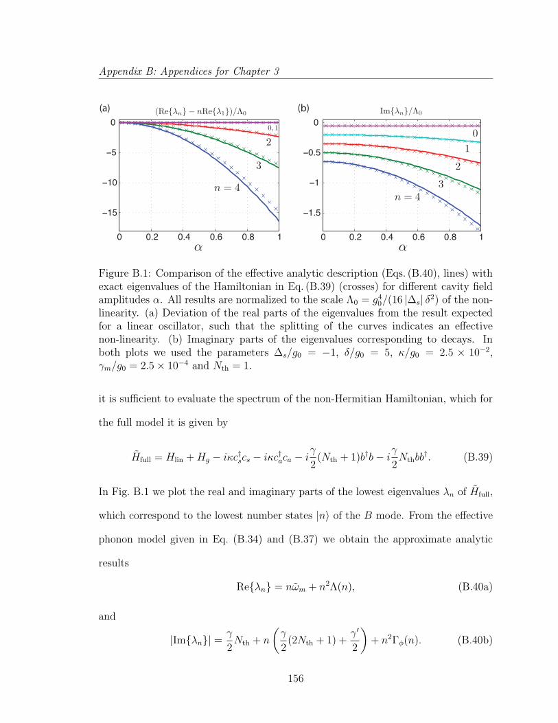
Appendix B: Appendices for Chapter 3
0 0.2 0.4 0.6 0.8 1
−1.5
−1
−0.5
0
0 0.2 0.4 0.6 0.8 1
−15
−10
−5
0(a) (b)
Figure B.1: Comparison of the effective analytic description (Eqs. (B.40), lines) withexact eigenvalues of the Hamiltonian in Eq. (B.39) (crosses) for different cavity fieldamplitudes α. All results are normalized to the scale Λ0 = g4
0/(16 |∆s| δ2) of the non-linearity. (a) Deviation of the real parts of the eigenvalues from the result expectedfor a linear oscillator, such that the splitting of the curves indicates an effectivenon-linearity. (b) Imaginary parts of the eigenvalues corresponding to decays. Inboth plots we used the parameters ∆s/g0 = −1, δ/g0 = 5, κ/g0 = 2.5 × 10⁻²,γm/g0 = 2.5× 10⁻⁴ and Nth = 1.
it is sufficient to evaluate the spectrum of the non-Hermitian Hamiltonian, which for
the full model it is given by
Hfull = Hlin +Hg − iκc†scs − iκc†aca − iγ
2(Nth + 1)b†b− iγ
2Nthbb
†. (B.39)
In Fig. B.1 we plot the real and imaginary parts of the lowest eigenvalues λn of Hfull,
which correspond to the lowest number states |n〉 of the B mode. From the effective
phonon model given in Eq. (B.34) and (B.37) we obtain the approximate analytic
results
Reλn = nωm + n2Λ(n), (B.40a)
and
|Imλn| =γ
2Nth + n
(γ
2(2Nth + 1) +
γ′
2
)+ n2Γφ(n). (B.40b)
156
Appendix B: Appendices for Chapter 3
We see a good agreement between these results for the effective model and the exact
numerics, both for the real and imaginary parts. Although there are some deviations
due to higher-order effects, the effective non-linear splitting (Fig. B.1(a)) is much
larger than the induced decoherence (Fig. B.1(b)), as is expected for the chosen
parameters. Hence, we conclude that the effective model accurately describes the
dynamics of the mechanical resonator, and that the effective phonon non-linearity
may serve as a basis for gate operations as discussed in the main text and in the
following section.
B.2 Phonon-phonon interactions
The derivation of the effective phonon nonlinearity, as outlined above for a single
resonator, can be easily adapted to two resonators as discussed in the main text. In
this case we have
H0 =∑
i=1,2
ωimb†ibi −∆sc
†scs −∆ac
†aca, (B.41)
and
Hg =g0
2
[cac†s(b†1 − b†2) + c†acs(b1 − b2)
]. (B.42)
After changing into the displaced representation to eliminate the driving field we
obtain the linearized Hamiltonian
Hlin = H0 +√
2(G(t)cab
†a +G∗(t)c†aba
), (B.43)
where ba = (b1 − b2)/√
2 and G(t) = g0α(t)/2. For similar mechanical frequencies
ω1m ' ω2
m = ωm the symmetric resonator mode is decoupled and we can simply repeat
the analysis from above by identifying b ≡ ba and replacing g0 by√
2g0.
157
Appendix B: Appendices for Chapter 3
For arbitrary ωi, we write the linear part of the Hamiltonian in its diagonal form
Hlin = −∆sc†scs − ∆aC
†C + ω1B†1B1 + ω2B
†2B2. (B.44)
As in the single-resonator case the cs mode is unaffected, but the ca mode now couples
to both b1 and b2. The resulting hybridized modes C, B± depend on the choice of
parameters ω1,2m ,∆a and G. For the case of interest, i.e. for a symmetric detuning
ω1,2m = −∆a ∓ δ, we obtain
C = cos(2Θ)ca − sin(2Θ)(B1 +B2)/√
2, (B.45)
B1 = cos2(Θ)b1 + sin(2Θ)ca/√
2− sin2(Θ)b2, (B.46)
B2 = cos2(Θ)b2 + sin(2Θ)ca/√
2− sin2(Θ)b1, (B.47)
where tan(2Θ) = −√
2|G|/δ. Therefore, for small Θ the modes B1,2 correspond to
the original mechanical resonator modes b1,2 and ωi ≈ ωim.
As above, we can now re-express the dissipation and the non-linear coupling Hg
in terms of C and B±. The modified mechanical dissipation terms are given
Lγ =∑
i=1,2
γ
2cos2(2Θ)Dth[Bi] +
κ
2sin2(2Θ)D[Bi], (B.48)
and for small Θ the optical decay rate γ′ = κ sin2(2Θ) is the same as given above
and in the main text. Using the decomposition of the non-linear coupling as done in
Eq. (B.15), we obtain
H(1)g =
g0√8
sin(2Θ)(cs + c†s
) (B†1B1 − B†2B2
), (B.49)
the contribution H(2)g vanishes and
H ′g =g0
2cos(2Θ)
(Cc†s(B
†1 − B†2) + H.c.
). (B.50)
158
Appendix B: Appendices for Chapter 3
We see that the structure and also the relative frequency scales are identical to the
corresponding terms discussed for the single resonator above. Therefore, under the
same conditions we can eliminate the cavity mode and obtain the effective phonon
master equation
ρm =− i[∑
i
ωiB†iBi + Λ(B†1B1 − B†2B2)2, ρm
]
+ ΓφD[(B†1B1 − B†2B2)]ρm + Lγρm.(B.51)
For small Θ this equation reduces to ME (8) in the main text and higher-order
corrections can be included in the same way as discussed for the single resonator
case.
159
Appendix C
Appendices for Chapter 4
This appendix describes the details of the perturbation theory and the derivation
of the effective Hamiltonian Heff and effective Lindblad operators. We describe the
situation both with and without a two-photon drive. Furthermore, we present the
results of a numerical simulation of the full dynamics of the gates to verify the results
found with perturbation theory and address the question of how strong a drive we
can allow for. In the end, this determines the gate time as described in the article.
Finally we discuss of the additional errors described in the final part of the article.
C.1 Perturbation theory
We will now give the details of the perturbation theory and the derivation of the
effective operators together with the success probabilitites, gate times and gate errors
(see Tab. C.1). Our perturbation theory is based on the effective operator formalism
described in Ref. [178].
160
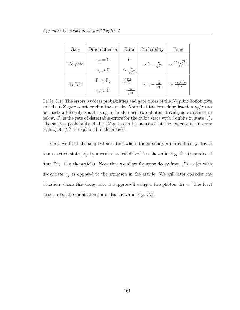
Appendix C: Appendices for Chapter 4
Gate Origin of error Error Probability Time
CZ-gateγg = 0
γg > 0
0
∼ γg
γ√C
∼ 1− 6√C
∼ 15π√Cγ
2Ω2
ToffoliΓi 6= Γj
γg > 0
. 0.3C
∼ γg
γ√C
∼ 1− 3√C
∼ 4π√Cγ
Ω2
Table C.1: The errors, success probabilities and gate times of the N -qubit Toffoli gateand the CZ-gate considered in the article. Note that the branching fraction γg/γ canbe made arbitrarily small using a far detuned two-photon driving as explained inbelow. Γi is the rate of detectable errors for the qubit state with i qubits in state |1〉.The success probability of the CZ-gate can be increased at the expense of an errorscaling of 1/C as explained in the article.
First, we treat the simplest situation where the auxiliary atom is directly driven
to an excited state |E〉 by a weak classical drive Ω as shown in Fig. C.1 (reproduced
from Fig. 1 in the article). Note that we allow for some decay from |E〉 → |g〉 with
decay rate γg as opposed to the situation in the article. We will later consider the
situation where this decay rate is suppressed using a two-photon drive. The level
structure of the qubit atoms are also shown in Fig. C.1.
161
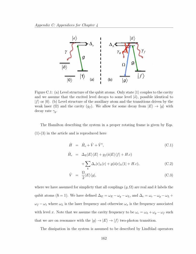
Appendix C: Appendices for Chapter 4
!!
!
!
!
Ω gf
!
!
!! !
!
!
(b) (a)
g
!!
!
!
!
Ω gf
!
!
!! !
!
!
(b) (a)
g
Figure C.1: (a) Level structure of the qubit atoms. Only state |1〉 couples to the cavityand we assume that the excited level decays to some level |o〉, possible identical to|f〉 or |0〉. (b) Level structure of the auxiliary atom and the transitions driven by theweak laser (Ω) and the cavity (gf ). We allow for some decay from |E〉 → |g〉 withdecay rate γg.
The Hamilton describing the system in a proper rotating frame is given by Eqs.
(1)-(3) in the article and is reproduced here
H = He + V + V †, (C.1)
He = ∆E|E〉〈E|+ gf (a|E〉〈f |+H.c)
+∑
k
∆e|e〉k〈e|+ g(a|e〉k〈1|+H.c), (C.2)
V =Ω
2|E〉〈g|, (C.3)
where we have assumed for simplicty that all couplings (g,Ω) are real and k labels the
qubit atoms ( = 1). We have defined ∆E = ωE −ωg −ωL, and ∆e = ωe −ωg −ωL +
ωf − ω1 where ωL is the laser frequency and otherwise ωx is the frequency associated
with level x. Note that we assume the cavity frequency to be ωc = ωL +ωg −ωf such
that we are on resonance with the |g〉 → |E〉 → |f〉 two-photon transition.
The dissipation in the system is assumed to be described by Lindblad operators
162
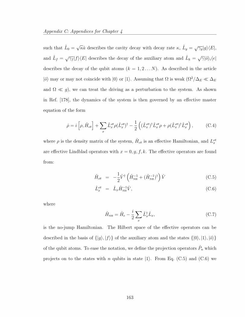
Appendix C: Appendices for Chapter 4
such that L0 =√κa describes the cavity decay with decay rate κ, Lg =
√γg|g〉〈E|,
and Lf =√γf |f〉〈E| describes the decay of the auxiliary atom and Lk =
√γ|o〉i〈e|
describes the decay of the qubit atoms (k = 1, 2 . . . N). As described in the article
|o〉 may or may not coincide with |0〉 or |1〉. Assuming that Ω is weak (Ω2/∆E ∆E
and Ω g), we can treat the driving as a perturbation to the system. As shown
in Ref. [178], the dynamics of the system is then governed by an effective master
equation of the form
ρ = i[ρ, Heff
]+∑
x
Leff
x ρ(Leff
x )† − 1
2
((Leff
x )†Leff
x ρ+ ρ(Leff
x )†Leff
x
), (C.4)
where ρ is the density matrix of the system, Heff is an effective Hamiltonian, and Leffx
are effective Lindblad operators with x = 0, g, f, k. The effective operators are found
from:
Heff = −1
2V †(H−1
NH + (H−1NH )†
)V (C.5)
Leff
x = LxH−1NH V , (C.6)
where
HNH = He −i
2
∑
x
L†xLx, (C.7)
is the no-jump Hamiltonian. The Hilbert space of the effective operators can be
described in the basis of |g〉, |f〉 of the auxiliary atom and the states |0〉, |1〉, |o〉
of the qubit atoms. To ease the notation, we define the projection operators Pn which
projects on to the states with n qubits in state |1〉. From Eq. (C.5) and (C.6) we
163
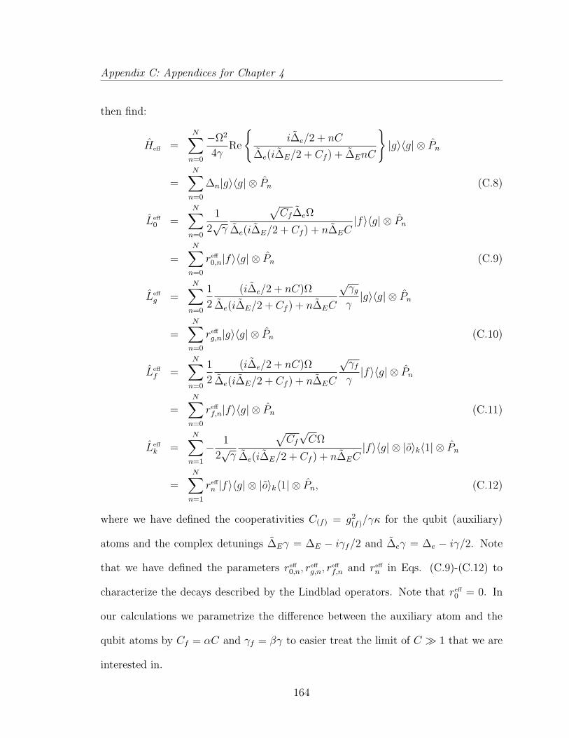
Appendix C: Appendices for Chapter 4
then find:
Heff =N∑
n=0
−Ω2
4γRe
i∆e/2 + nC
∆e(i∆E/2 + Cf ) + ∆EnC
|g〉〈g| ⊗ Pn
=N∑
n=0
∆n|g〉〈g| ⊗ Pn (C.8)
Leff
0 =N∑
n=0
1
2√γ
√Cf∆eΩ
∆e(i∆E/2 + Cf ) + n∆EC|f〉〈g| ⊗ Pn
=N∑
n=0
reff
0,n|f〉〈g| ⊗ Pn (C.9)
Leff
g =N∑
n=0
1
2
(i∆e/2 + nC)Ω
∆e(i∆E/2 + Cf ) + n∆EC
√γg
γ|g〉〈g| ⊗ Pn
=N∑
n=0
reff
g,n|g〉〈g| ⊗ Pn (C.10)
Leff
f =N∑
n=0
1
2
(i∆e/2 + nC)Ω
∆e(i∆E/2 + Cf ) + n∆EC
√γf
γ|f〉〈g| ⊗ Pn
=N∑
n=0
reff
f,n|f〉〈g| ⊗ Pn (C.11)
Leff
k =N∑
n=1
− 1
2√γ
√Cf√CΩ
∆e(i∆E/2 + Cf ) + n∆EC|f〉〈g| ⊗ |o〉k〈1| ⊗ Pn
=N∑
n=1
reff
n |f〉〈g| ⊗ |o〉k〈1| ⊗ Pn, (C.12)
where we have defined the cooperativities C(f) = g2(f)/γκ for the qubit (auxiliary)
atoms and the complex detunings ∆Eγ = ∆E − iγf/2 and ∆eγ = ∆e − iγ/2. Note
that we have defined the parameters reff0,n, r
effg,n, r
efff,n and reff
n in Eqs. (C.9)-(C.12) to
characterize the decays described by the Lindblad operators. Note that reff0 = 0. In
our calculations we parametrize the difference between the auxiliary atom and the
qubit atoms by Cf = αC and γf = βγ to easier treat the limit of C 1 that we are
interested in.
164
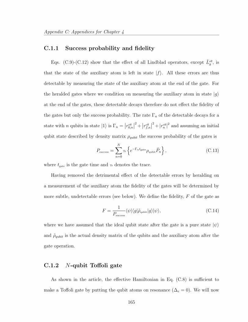
Appendix C: Appendices for Chapter 4
C.1.1 Success probability and fidelity
Eqs. (C.9)-(C.12) show that the effect of all Lindblad operators, except Leffg , is
that the state of the auxiliary atom is left in state |f〉. All these errors are thus
detectable by measuring the state of the auxiliary atom at the end of the gate. For
the heralded gates where we condition on measuring the auxiliary atom in state |g〉
at the end of the gates, these detectable decays therefore do not effect the fidelity of
the gates but only the success probability. The rate Γn of the detectable decays for a
state with n qubits in state |1〉 is Γn =∣∣reff
0,n
∣∣2 +∣∣refff,n
∣∣2 + |reffn |2 and assuming an initial
qubit state described by density matrix ρqubit the success probability of the gates is
Psuccess =N∑
n=0
Tr
e−ΓntgateρqubitPn
, (C.13)
where tgate is the gate time and Tr denotes the trace.
Having removed the detrimental effect of the detectable errors by heralding on
a measurement of the auxiliary atom the fidelity of the gates will be determined by
more subtle, undetectable errors (see below). We define the fidelity, F of the gate as
F =1
Psuccess
〈ψ|〈g|ρqubit|g〉|ψ〉, (C.14)
where we have assumed that the ideal qubit state after the gate is a pure state |ψ〉
and ρqubit is the actual density matrix of the qubits and the auxiliary atom after the
gate operation.
C.1.2 N-qubit Toffoli gate
As shown in the article, the effective Hamiltonian in Eq. (C.8) is sufficient to
make a Toffoli gate by putting the qubit atoms on resonance (∆e = 0). We will now
165
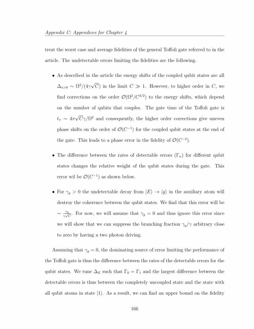
Appendix C: Appendices for Chapter 4
treat the worst case and average fidelities of the general Toffoli gate referred to in the
article. The undetectable errors limiting the fidelities are the following.
• As described in the article the energy shifts of the coupled qubit states are all
∆n>0 ∼ Ω2/(4γ√C) in the limit C 1. However, to higher order in C, we
find corrections on the order O(Ω2/C3/2) to the energy shifts, which depend
on the number of qubits that couples. The gate time of the Toffoli gate is
tT ∼ 4π√Cγ/Ω2 and consequently, the higher order corrections give uneven
phase shifts on the order of O(C−1) for the coupled qubit states at the end of
the gate. This leads to a phase error in the fidelity of O(C−2).
• The difference between the rates of detectable errors (Γn) for different qubit
states changes the relative weight of the qubit states during the gate. This
error wil be O(C−1) as shown below.
• For γg > 0 the undetectable decay from |E〉 → |g〉 in the auxiliary atom will
destroy the coherence between the qubit states. We find that this error will be
∼ γg
γ√C
. For now, we will assume that γg = 0 and thus ignore this error since
we will show that we can suppress the branching fraction γg/γ arbitrary close
to zero by having a two photon driving.
Assuming that γg = 0, the dominating source of error limiting the performance of
the Toffoli gate is thus the difference between the rates of the detectable errors for the
qubit states. We tune ∆E such that Γ0 = Γ1 and the largest difference between the
detectable errors is thus between the completely uncoupled state and the state with
all qubit atoms in state |1〉. As a result, we can find an upper bound on the fidelity
166
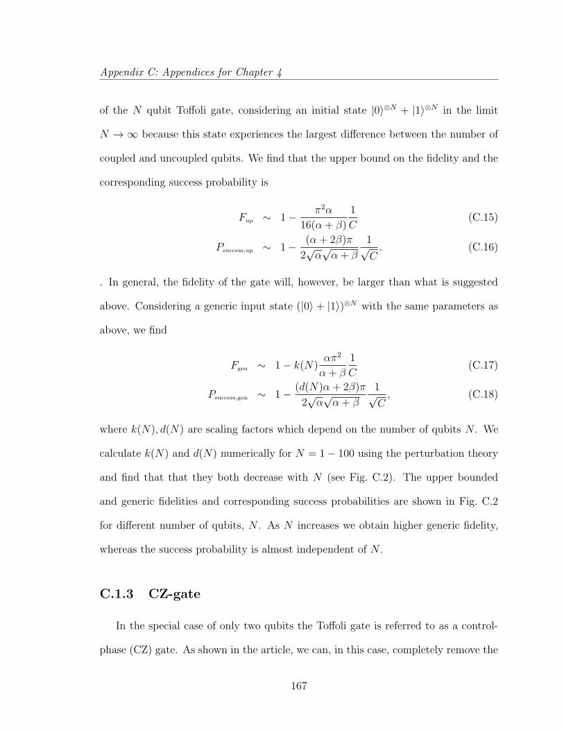
Appendix C: Appendices for Chapter 4
of the N qubit Toffoli gate, considering an initial state |0〉⊗N + |1〉⊗N in the limit
N → ∞ because this state experiences the largest difference between the number of
coupled and uncoupled qubits. We find that the upper bound on the fidelity and the
corresponding success probability is
Fup ∼ 1− π2α
16(α + β)
1
C(C.15)
Psuccess,up ∼ 1− (α + 2β)π
2√α√α + β
1√C. (C.16)
. In general, the fidelity of the gate will, however, be larger than what is suggested
above. Considering a generic input state (|0〉 + |1〉)⊗N with the same parameters as
above, we find
Fgen ∼ 1− k(N)απ2
α + β
1
C(C.17)
Psuccess,gen ∼ 1− (d(N)α + 2β)π
2√α√α + β
1√C, (C.18)
where k(N), d(N) are scaling factors which depend on the number of qubits N . We
calculate k(N) and d(N) numerically for N = 1− 100 using the perturbation theory
and find that that they both decrease with N (see Fig. C.2). The upper bounded
and generic fidelities and corresponding success probabilities are shown in Fig. C.2
for different number of qubits, N . As N increases we obtain higher generic fidelity,
whereas the success probability is almost independent of N .
C.1.3 CZ-gate
In the special case of only two qubits the Toffoli gate is referred to as a control-
phase (CZ) gate. As shown in the article, we can, in this case, completely remove the
167

Appendix C: Appendices for Chapter 4
100 101 102 10310−6
10−5
10−4
10−3
10−2
10−1
100
Cooperativity
Erro
r
UpperN=5N=10N=15
(a)
100 101 102 103
10−1
100
Cooperativity
1−P su
cces
s
UpperN=5N=10N=15
(b) (b)
Figure C.2: (a) Gate error of the Toffoli for different initial states as a function ofcooperativity. We have plotted the generic error for N = 5, 10, and 15 and the upperbound of the error. Note that the generic error decreases as N increases. We havefixed ∆ such that Γ0 = Γ1 and have assumed that α = β = 1. (b) The failureprobabilities 1−Psuccess,up and 1−Psuccess,gen as a function of cooperativity. 1−Psuccess,gen
is plotted for N = 5, 10, 15. We have used the same assumptions as in (a). In general,the failure probability only have a weak dependence on N . Note that the line for1− Psuccess, gen, N = 5 coincides with 1− Psuccess,up.
errors from the gate by choosing the detunings ∆E and ∆e such that Γ0 = Γ1 = Γ2
and combining it with single qubit rotations we can ensure the right phase evolution.
In the general case where α, β 6= 1, the detunings ∆e and ∆E are
∆E =γ
2
√β√
4αC + β (C.19)
∆e =αCγ2
2∆E
. (C.20)
The success probability of the gate is then
Psuccess ' 1− π8β2 + 6βα + α2
8β3/2√α
1√C, (C.21)
and we find that the gate time is tCZ ' γπ√α(α+2β)(α+4β)
2β3/2Ω2
√C in the limit C 1.
168
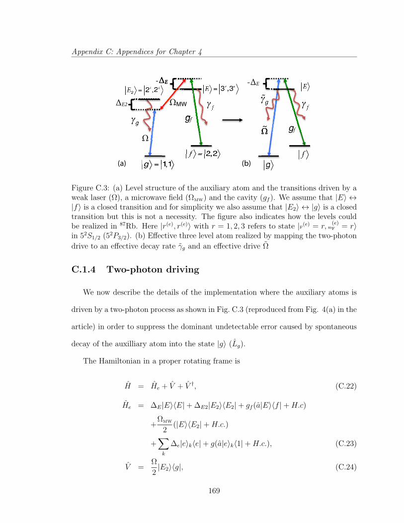
Appendix C: Appendices for Chapter 4
!!!!!!!!
!
!
!
!
Ω
gf!
-ΔE
gfgfg
-ΔE
ΩMW
!
!!!!!!ΔE2 !
!
!
!
!
gf!
-ΔE
Ω ΩΩΩΩ~
!
!
!
!
(a) (b)
Figure C.3: (a) Level structure of the auxiliary atom and the transitions driven by aweak laser (Ω), a microwave field (ΩMW) and the cavity (gf ). We assume that |E〉 ↔|f〉 is a closed transition and for simplicity we also assume that |E2〉 ↔ |g〉 is a closedtransition but this is not a necessity. The figure also indicates how the levels couldbe realized in 87Rb. Here |r(e), r(e)〉 with r = 1, 2, 3 refers to state |F(e) = r, m
(e)F = r〉
in 52S1/2 (52P3/2). (b) Effective three level atom realized by mapping the two-photon
drive to an effective decay rate γg and an effective drive Ω
C.1.4 Two-photon driving
We now describe the details of the implementation where the auxiliary atoms is
driven by a two-photon process as shown in Fig. C.3 (reproduced from Fig. 4(a) in the
article) in order to suppress the dominant undetectable error caused by spontaneous
decay of the auxilliary atom into the state |g〉 (Lg).
The Hamiltonian in a proper rotating frame is
H = He + V + V †, (C.22)
He = ∆E|E〉〈E|+∆E2|E2〉〈E2|+ gf (a|E〉〈f |+H.c)
+ΩMW
2(|E〉〈E2|+H.c.)
+∑
k
∆e|e〉k〈e|+ g(a|e〉k〈1|+H.c.), (C.23)
V =Ω
2|E2〉〈g|, (C.24)
169
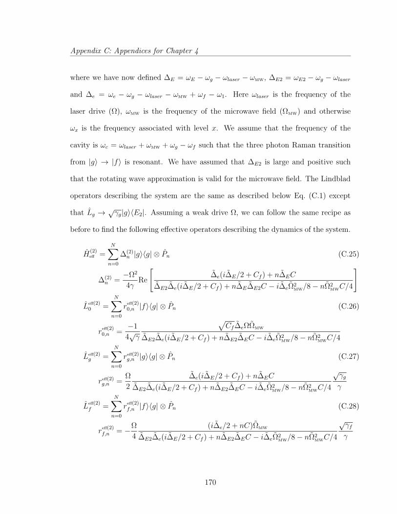
Appendix C: Appendices for Chapter 4
where we have now defined ∆E = ωE − ωg − ωlaser − ωMW, ∆E2 = ωE2 − ωg − ωlaser
and ∆e = ωe − ωg − ωlaser − ωMW + ωf − ω1. Here ωlaser is the frequency of the
laser drive (Ω), ωMW is the frequency of the microwave field (ΩMW) and otherwise
ωx is the frequency associated with level x. We assume that the frequency of the
cavity is ωc = ωlaser + ωMW + ωg − ωf such that the three photon Raman transition
from |g〉 → |f〉 is resonant. We have assumed that ∆E2 is large and positive such
that the rotating wave approximation is valid for the microwave field. The Lindblad
operators describing the system are the same as described below Eq. (C.1) except
that Lg → √γg|g〉〈E2|. Assuming a weak drive Ω, we can follow the same recipe as
before to find the following effective operators describing the dynamics of the system.
H(2)eff =
N∑
n=0
∆(2)n |g〉〈g| ⊗ Pn (C.25)
∆(2)n =
−Ω2
4γRe
[∆e(i∆E/2 + Cf ) + n∆EC
∆E2∆e(i∆E/2 + Cf ) + n∆E∆E2C − i∆eΩ2MW/8− nΩ2
MWC/4
]
Leff(2)0 =
N∑
n=0
reff(2)0,n |f〉〈g| ⊗ Pn (C.26)
reff(2)0,n =
−1
4√γ
√Cf∆eΩΩMW
∆E2∆e(i∆E/2 + Cf ) + n∆E2∆EC − i∆eΩ2MW/8− nΩ2
MWC/4
Leff(2)g =
N∑
n=0
reff(2)g,n |g〉〈g| ⊗ Pn (C.27)
reff(2)g,n =
Ω
2
∆e(i∆E/2 + Cf ) + n∆EC
∆E2∆e(i∆E/2 + Cf ) + n∆E2∆EC − i∆eΩ2MW/8− nΩ2
MWC/4
√γg
γ
Leff(2)f =
N∑
n=0
reff(2)f,n |f〉〈g| ⊗ Pn (C.28)
reff(2)f,n = −Ω
4
(i∆e/2 + nC)ΩMW
∆E2∆e(i∆E/2 + Cf ) + n∆E2∆EC − i∆eΩ2MW/8− nΩ2
MWC/4
√γf
γ
170
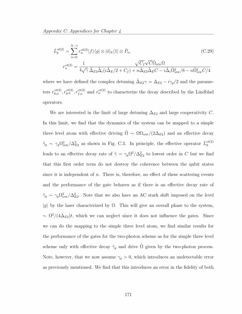
Appendix C: Appendices for Chapter 4
Leff(2)k =
N−1∑
n=0
reff(2)n |f〉〈g| ⊗ |o〉k〈1| ⊗ Pn, (C.29)
reff(2)n =
1
4√γ
√Cf√CΩMWΩ
∆E2∆e(i∆E/2 + Cf ) + n∆E2∆EC − i∆eΩ2MW/8− nΩ2
MWC/4
where we have defined the complex detuning ∆E2γ = ∆E2 − iγg/2 and the parame-
ters reff(2)0,n , r
eff(2)g,n , r
eff(2)f,n and r
eff(2)n to characterize the decay described by the Lindblad
operators.
We are interested in the limit of large detuning ∆E2 and large cooperativity C.
In this limit, we find that the dynamics of the system can be mapped to a simple
three level atom with effective driving Ω ∼ ΩΩMW/(2∆E2) and an effective decay
γg ∼ γgΩ2MW/∆
2E2 as shown in Fig. C.3. In principle, the effective operator L
eff(2)0
leads to an effective decay rate of γ = γgΩ2/∆2
E2 to lowest order in C but we find
that this first order term do not destroy the coherence between the qubit states
since it is independent of n. There is, therefore, no effect of these scattering events
and the performance of the gate behaves as if there is an effective decay rate of
γg ∼ γgΩ2MW/∆
2E2. Note that we also have an AC stark shift imposed on the level
|g〉 by the laser characterized by Ω. This will give an overall phase to the system,
∼ Ω2/(4∆E2)t, which we can neglect since it does not influence the gates. Since
we can do the mapping to the simple three level atom, we find similar results for
the performance of the gates for the two-photon scheme as for the simple three level
scheme only with effective decay γg and drive Ω given by the two-photon process.
Note, however, that we now assume γg > 0, which introduces an undetectable error
as previously mentioned. We find that this introduces an error in the fidelity of both
171
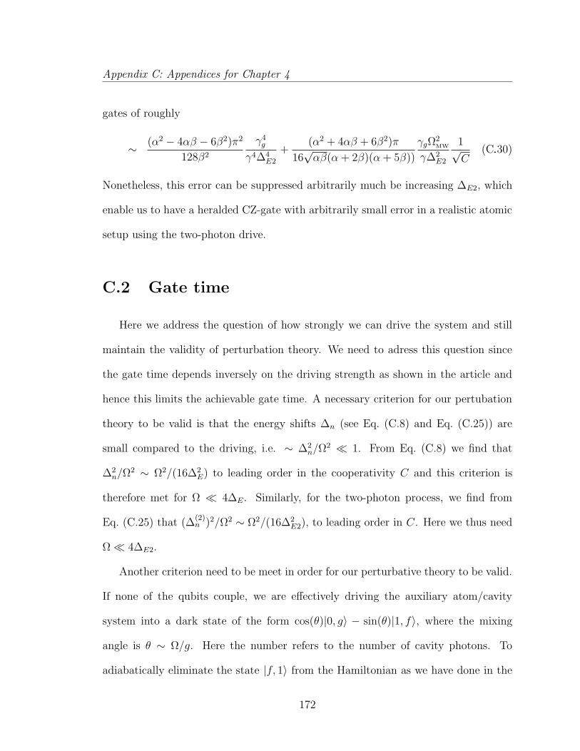
Appendix C: Appendices for Chapter 4
gates of roughly
∼ (α2 − 4αβ − 6β2)π2
128β2
γ4g
γ4∆4E2
+(α2 + 4αβ + 6β2)π
16√αβ(α + 2β)(α + 5β))
γgΩ2MW
γ∆2E2
1√C
.(C.30)
Nonetheless, this error can be suppressed arbitrarily much be increasing ∆E2, which
enable us to have a heralded CZ-gate with arbitrarily small error in a realistic atomic
setup using the two-photon drive.
C.2 Gate time
Here we address the question of how strongly we can drive the system and still
maintain the validity of perturbation theory. We need to adress this question since
the gate time depends inversely on the driving strength as shown in the article and
hence this limits the achievable gate time. A necessary criterion for our pertubation
theory to be valid is that the energy shifts ∆n (see Eq. (C.8) and Eq. (C.25)) are
small compared to the driving, i.e. ∼ ∆2n/Ω
2 1. From Eq. (C.8) we find that
∆2n/Ω
2 ∼ Ω2/(16∆2E) to leading order in the cooperativity C and this criterion is
therefore met for Ω 4∆E. Similarly, for the two-photon process, we find from
Eq. (C.25) that (∆(2)n )2/Ω2 ∼ Ω2/(16∆2
E2), to leading order in C. Here we thus need
Ω 4∆E2.
Another criterion need to be meet in order for our perturbative theory to be valid.
If none of the qubits couple, we are effectively driving the auxiliary atom/cavity
system into a dark state of the form cos(θ)|0, g〉 − sin(θ)|1, f〉, where the mixing
angle is θ ∼ Ω/g. Here the number refers to the number of cavity photons. To
adiabatically eliminate the state |f, 1〉 from the Hamiltonian as we have done in the
172
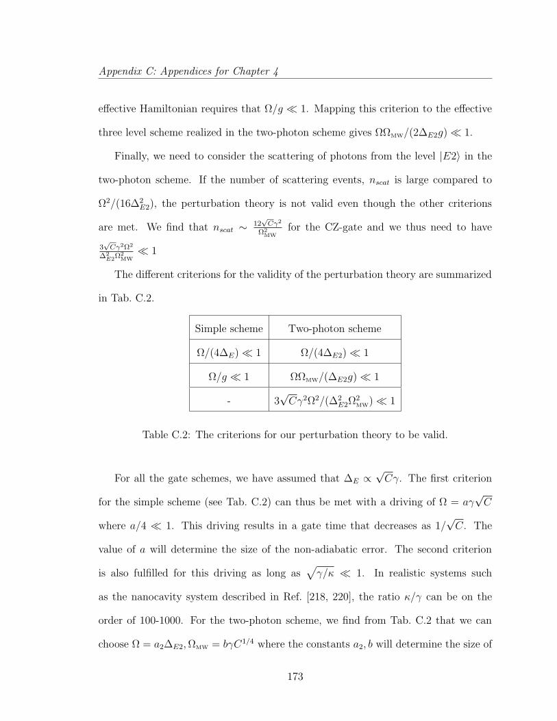
Appendix C: Appendices for Chapter 4
effective Hamiltonian requires that Ω/g 1. Mapping this criterion to the effective
three level scheme realized in the two-photon scheme gives ΩΩMW/(2∆E2g) 1.
Finally, we need to consider the scattering of photons from the level |E2〉 in the
two-photon scheme. If the number of scattering events, nscat is large compared to
Ω2/(16∆2E2), the perturbation theory is not valid even though the other criterions
are met. We find that nscat ∼ 12√Cγ2
Ω2MW
for the CZ-gate and we thus need to have
3√Cγ2Ω2
∆2E2Ω2
MW 1
The different criterions for the validity of the perturbation theory are summarized
in Tab. C.2.
Simple scheme Two-photon scheme
Ω/(4∆E) 1 Ω/(4∆E2) 1
Ω/g 1 ΩΩMW/(∆E2g) 1
- 3√Cγ2Ω2/(∆2
E2Ω2MW) 1
Table C.2: The criterions for our perturbation theory to be valid.
For all the gate schemes, we have assumed that ∆E ∝√Cγ. The first criterion
for the simple scheme (see Tab. C.2) can thus be met with a driving of Ω = aγ√C
where a/4 1. This driving results in a gate time that decreases as 1/√C. The
value of a will determine the size of the non-adiabatic error. The second criterion
is also fulfilled for this driving as long as√γ/κ 1. In realistic systems such
as the nanocavity system described in Ref. [218, 220], the ratio κ/γ can be on the
order of 100-1000. For the two-photon scheme, we find from Tab. C.2 that we can
choose Ω = a2∆E2,ΩMW = bγC1/4 where the constants a2, b will determine the size of
173
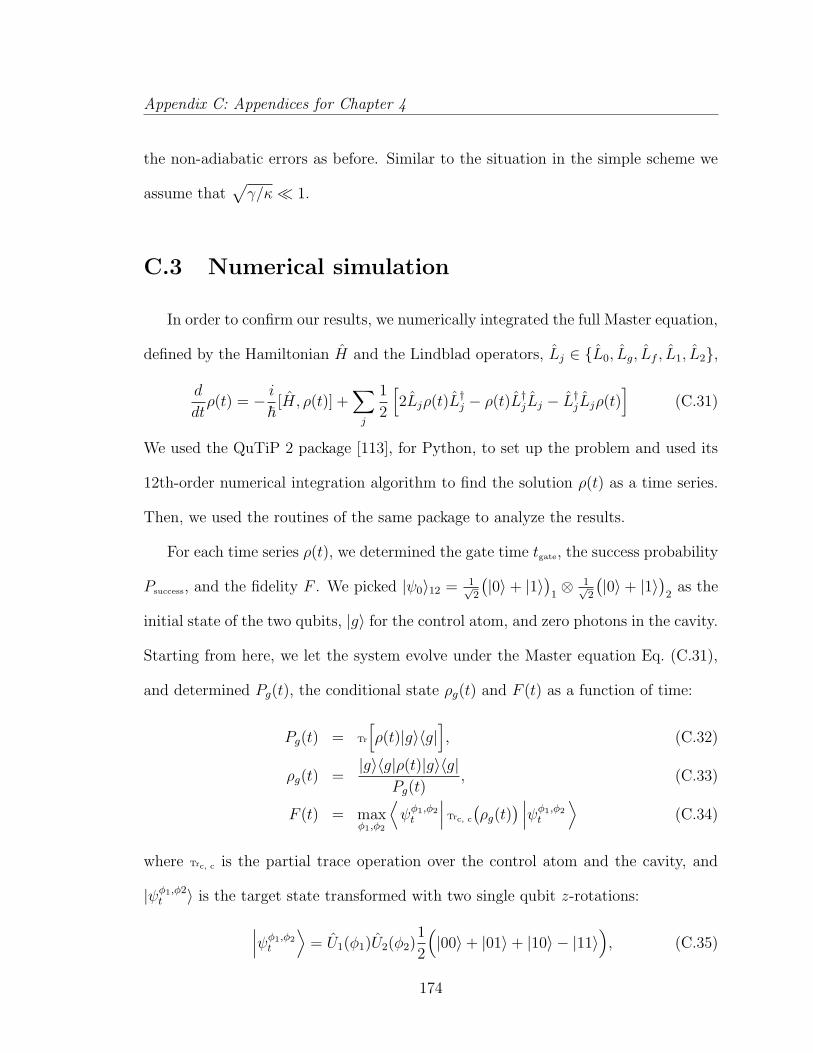
Appendix C: Appendices for Chapter 4
the non-adiabatic errors as before. Similar to the situation in the simple scheme we
assume that√γ/κ 1.
C.3 Numerical simulation
In order to confirm our results, we numerically integrated the full Master equation,
defined by the Hamiltonian H and the Lindblad operators, Lj ∈ L0, Lg, Lf , L1, L2,
d
dtρ(t) = − i
~[H, ρ(t)] +
∑
j
1
2
[2Ljρ(t)L†j − ρ(t)L†jLj − L†jLjρ(t)
](C.31)
We used the QuTiP 2 package [113], for Python, to set up the problem and used its
12th-order numerical integration algorithm to find the solution ρ(t) as a time series.
Then, we used the routines of the same package to analyze the results.
For each time series ρ(t), we determined the gate time tgate, the success probability
Psuccess, and the fidelity F . We picked |ψ0〉12 = 1√2
(|0〉+ |1〉
)1⊗ 1√
2
(|0〉+ |1〉
)2
as the
initial state of the two qubits, |g〉 for the control atom, and zero photons in the cavity.
Starting from here, we let the system evolve under the Master equation Eq. (C.31),
and determined Pg(t), the conditional state ρg(t) and F (t) as a function of time:
Pg(t) = Tr
[ρ(t)|g〉〈g|
], (C.32)
ρg(t) =|g〉〈g|ρ(t)|g〉〈g|
Pg(t), (C.33)
F (t) = maxφ1,φ2
⟨ψφ1,φ2t
∣∣∣ Trc, c
(ρg(t)
) ∣∣∣ψφ1,φ2t
⟩(C.34)
where Trc, c is the partial trace operation over the control atom and the cavity, and
|ψφ1,φ2t 〉 is the target state transformed with two single qubit z-rotations:
∣∣∣ψφ1,φ2t
⟩= U1(φ1)U2(φ2)
1
2
(|00〉+ |01〉+ |10〉 − |11〉
), (C.35)
174
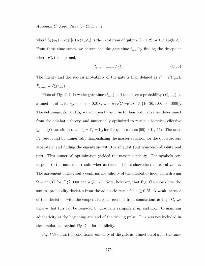
Appendix C: Appendices for Chapter 4
where Uk(φk) = exp [i|1〉k〈1|kφk] is the z-rotation of qubit k (= 1, 2) by the angle φk.
From these time series, we determined the gate time tgate by finding the timepoint
where F (t) is maximal,
tgate = argmax
tF (t) (C.36)
The fidelity and the success probability of the gate is then defined as F = F (tgate),
Psuccess = Pg(tgate).
Plots of Fig. C.4 show the gate time (tgate) and the success probability (Psuccess) as
a function of a, for γg = 0, γ = 0.01κ, Ω = aγ√C with C ∈ 10, 30, 100, 300, 1000.
The detunings, ∆E and ∆e were chosen to be close to their optimal value, determined
from the adiabatic theory, and numerically optimized to result in identical effective
|g〉 → |f〉 transition rates Γ0 = Γ1 = Γ2 for the qubit sectors |00〉, |01〉, |11〉. The rates
Γj were found by numerically diagonalizing the master equation for the qubit sectors
separately, and finding the eigenvalue with the smallest (but non-zero) absolute real
part. This numerical optimization yielded the maximal fidelity. The symbols cor-
respond to the numerical result, whereas the solid lines show the theoretical values.
The agreement of the results confirms the validity of the adiabatic theory for a driving
Ω = aγ√C for C . 1000 and a . 0.25. Note, however, that Fig. C.4 shows how the
success probability deviates from the adiabatic result for a & 0.25. A weak increase
of this deviation with the cooperativity is seen but from simulations at high C, we
believe that this can be removed by gradually ramping Ω up and down to maintain
adiabaticity at the beginning and end of the driving pulse. This was not included in
the simulations behind Fig. C.4 for simplicity.
Fig. C.5 shows the conditional infidelity of the gate as a function of a for the same
175
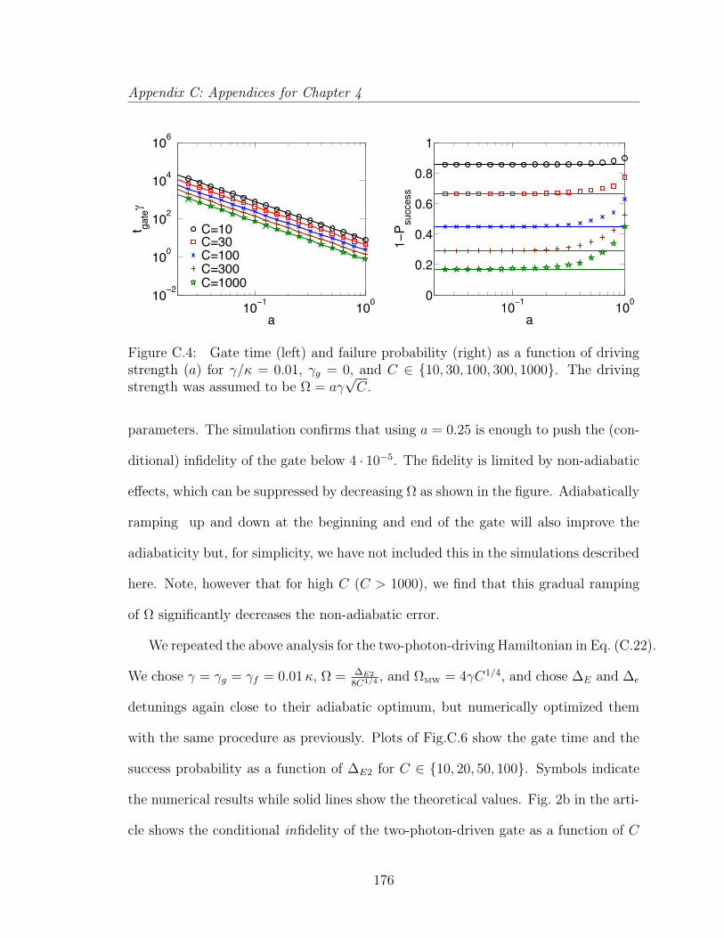
Appendix C: Appendices for Chapter 4
10−1 10010−2
100
102
104
106
a
t gateγ
C=10C=30C=100C=300C=1000
C=10C=30C=100C=300C=1000
10−1
100
0
0.2
0.4
0.6
0.8
1
a
1−
Psu
cce
ss
Figure C.4: Gate time (left) and failure probability (right) as a function of drivingstrength (a) for γ/κ = 0.01, γg = 0, and C ∈ 10, 30, 100, 300, 1000. The drivingstrength was assumed to be Ω = aγ
√C.
parameters. The simulation confirms that using a = 0.25 is enough to push the (con-
ditional) infidelity of the gate below 4 · 10−5. The fidelity is limited by non-adiabatic
effects, which can be suppressed by decreasing Ω as shown in the figure. Adiabatically
ramping up and down at the beginning and end of the gate will also improve the
adiabaticity but, for simplicity, we have not included this in the simulations described
here. Note, however that for high C (C > 1000), we find that this gradual ramping
of Ω significantly decreases the non-adiabatic error.
We repeated the above analysis for the two-photon-driving Hamiltonian in Eq. (C.22).
We chose γ = γg = γf = 0.01κ, Ω = ∆E2
8C1/4 , and ΩMW = 4γC1/4, and chose ∆E and ∆e
detunings again close to their adiabatic optimum, but numerically optimized them
with the same procedure as previously. Plots of Fig.C.6 show the gate time and the
success probability as a function of ∆E2 for C ∈ 10, 20, 50, 100. Symbols indicate
the numerical results while solid lines show the theoretical values. Fig. 2b in the arti-
cle shows the conditional infidelity of the two-photon-driven gate as a function of C
176

Appendix C: Appendices for Chapter 4
10−1 10010−1010−810−610−410−2100
a
Erro
r
C=10C=30C=100C=300C=1000
Figure C.5: Conditional infidelity of the gate as a function of the driving strength(a) for γ/κ = 0.01, γg = 0, and C ∈ 10, 30, 100, 300, 1000. The shaded region (at∼ 10−6) shows the limit of numerical accuracy. The driving strength was assumed tobe Ω = aγ
√C.
for the same choice of parameters. With these results, we confirm that by increasing
∆E2 we can lower the infidelity error to an arbitrary small level. The gate time is
a constant of the cooperativity since we have increased ΩMW as C1/4 in the simu-
lations. We do see some deviation from the analytical results due to non-adiabatic
effects, which could be suppressed by decreasing Ω at the expense of an increase in
the gate time. Finally a gradual ramping of Ω could also decrease the non-adiabatic
errors but for simplicity, we have not included this in the simulations.
C.4 Additional errors
There are some additional errors in a realistic atomic setup that we have not
treated in detail so far. Here we estimate the dominant errors and determine under
which conditions, they can be sufficiently suppressed such that they do not limit the
performance of the gates. We assume a realistic atomic setup where 87Rb atoms are
177
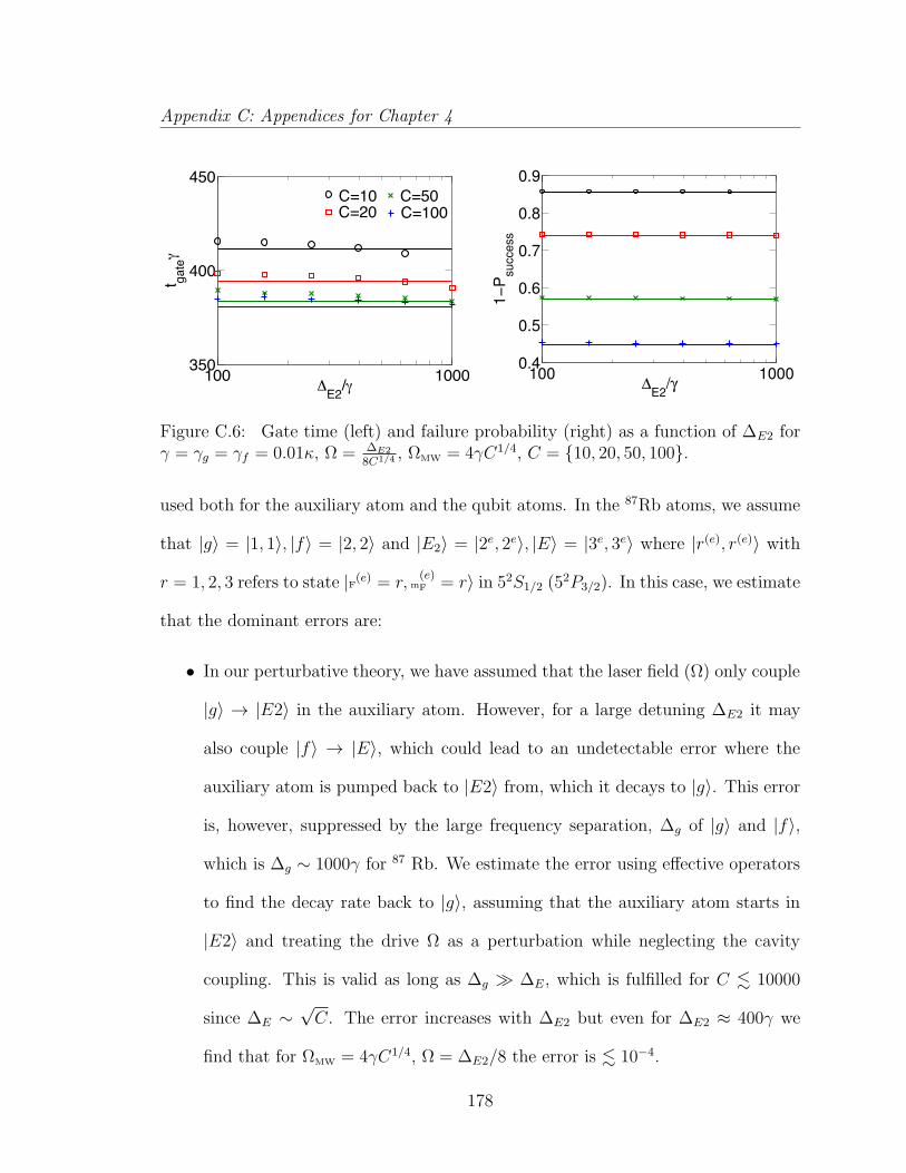
Appendix C: Appendices for Chapter 4
100 1000350
400
450
ΔE2/γ
t gateγ
data1data2data3
C=10C=20
C=50C=100
data8
100 10000.4
0.5
0.6
0.7
0.8
0.9
∆E2
/γ
1−
Psuccess
Figure C.6: Gate time (left) and failure probability (right) as a function of ∆E2 forγ = γg = γf = 0.01κ, Ω = ∆E2
8C1/4 , ΩMW = 4γC1/4, C = 10, 20, 50, 100.
used both for the auxiliary atom and the qubit atoms. In the 87Rb atoms, we assume
that |g〉 = |1, 1〉, |f〉 = |2, 2〉 and |E2〉 = |2e, 2e〉, |E〉 = |3e, 3e〉 where |r(e), r(e)〉 with
r = 1, 2, 3 refers to state |F(e) = r, m(e)F = r〉 in 52S1/2 (52P3/2). In this case, we estimate
that the dominant errors are:
• In our perturbative theory, we have assumed that the laser field (Ω) only couple
|g〉 → |E2〉 in the auxiliary atom. However, for a large detuning ∆E2 it may
also couple |f〉 → |E〉, which could lead to an undetectable error where the
auxiliary atom is pumped back to |E2〉 from, which it decays to |g〉. This error
is, however, suppressed by the large frequency separation, ∆g of |g〉 and |f〉,
which is ∆g ∼ 1000γ for 87 Rb. We estimate the error using effective operators
to find the decay rate back to |g〉, assuming that the auxiliary atom starts in
|E2〉 and treating the drive Ω as a perturbation while neglecting the cavity
coupling. This is valid as long as ∆g ∆E, which is fulfilled for C . 10000
since ∆E ∼√C. The error increases with ∆E2 but even for ∆E2 ≈ 400γ we
find that for ΩMW = 4γC1/4, Ω = ∆E2/8 the error is . 10−4.
178

Appendix C: Appendices for Chapter 4
• The microwave might also couple the ground states |0〉− |1〉 of the qubit atoms
and the ground states |g〉 − |f〉 of the auxiliary atom. The coupling of |0〉 − |1〉
means that the qubit atoms also couple to the cavity even though they are in
state |0〉. We estimate the error from this to be on the order of Ω2MW/(∆g −
(∆E2 − ∆E + ∆2→3))2 where ∆2→3 is the splitting between |E2〉 and |E〉. For
87Rb, ∆2→3 ≈ 44γ. Below we argue that we need ∆E < 0. Since ∆E ≈ −√Cγ
this error will increase slowly with cooperativity but it is suppressed by ∆g.
For ΩMW = 4γC1/4, we find that the error is . 10−4 for C . 1000 even for
∆E2 ≈ 400γ. The errors from the coupling of the states |g〉−|f〉 in the auxiliary
atom will likewise be suppressed by the large energy splitting ∆g. These errors
can also be further suppressed by decreasing ΩMW at the cost of a larger gate
time.
The above errors can be highly suppressed using e.g.88Sr, 138Ba+ or 40Ca+ instead
of 87Rb. For these atoms, the ground states can be encoded in the S0 and P0 man-
ifoldes for 88Sr and the S1/2 and D3/5 manifolds for 138Ba+ and 40Ca+, which have
separations at optical frequencies between the stable states.
A final error that we will consider is that the transition |E〉 ↔ |f〉 will not be
completely closed if the cavity is linearly polarized. This will, e.g. be the case for
the system in Ref. [218]. Such a cavity also couples |f〉 to the states |1e, 1e〉, |2e, 1e〉
and |3e, 1e〉. From |1e, 1e〉 and |2e, 1e〉 there might be an undetectable decay back
to |g〉, which will introduce an error ∝ 1/√C in the gates. The probability of an
undetectable decay from these states should be compared to the probability of the
detectable decays where the cavity photon is scattered of the qubit atoms instead.
179
Appendix C: Appendices for Chapter 4
For 87Rb, we estimate this error by compairing the strengths of the effective couplings
from |f〉 to |1e, 1e〉 and |2e, 1e〉 with a subsequent decay to |g〉 with the strength of the
effective coupling from |1〉 to |e〉 in the qubit atoms with a subsequent decay back to
|1〉. The latter process has a detuning of ∆E while the first two are additional detuned
by the energy gaps between |3e, 3e〉 and |1e, 1e〉 and |3e, 3e〉 and |2e, 1e〉 respectively,
assuming that ∆E < 0. We find that since |∆E| grows as√C the error increases from
∼ 5 · 10−5 at C = 1 to a maximum value of ∼ 2 · 10−3 for C ∼ 3000 for which ∆E is
comparable to the extra detunings of the |1e, 1e〉 and |2e, 1e〉 transitions compared to
the |e〉 transition. For C > 3000 the error decreases as 1/√C. Note that this error
could be removed by making a 4 photon drive from |g〉 to |E〉 by letting |g〉 = |1,−1〉.
Another approach is to consider other atoms such as 40Ca+, with more favorable
levelstructures. The state |g〉 could be encoded in the 32D5/2 subspace while the
state |f〉 could be encoded in the 42S1/2 subspace and similarly for the qubit states
|0〉 and |1〉. In such a setup, we will have separations of optical frequencies between
the qubit states and we can remove the decay from the excited state back to |g〉 by,
e.g. driving from 32D5/2 to 42P1/2 through 32D3/2.
180
Appendix D
Appendices for Chapter 5
D.1 Error analysis of the single-photon scheme
The setup of the single-photon scheme is described in Sec. 5.3.1. The single photon
detectors are assumed to have a dark count probability of Pdark and an efficiency of ηd
while the transmission efficiency of the fibers is denoted ηf. As described in Sec. 5.2,
the probability of an emitter to go from the excited state, |e〉 to the ground state |1〉
is Pphot while the excitation probability is ε2. The scheme is conditioned on a single
click at the central station. Depending on which detector gave the click, a single
qubit rotation can be employed such that ideally the state |Ψ+〉 is created. Going
through all the possibilities of obtaining a single click at the central station, we find
that the density matrix following a single click, and possible subsequent single qubit
rotations, is
ρ1click = F1|Ψ+〉〈Ψ+|+ α1|Φ+〉〈Φ+|+ α1|Φ−〉〈Φ−|
+β1|Ψ−〉〈Ψ−|+ α1|00〉〈00|+ β1|11〉〈11|, (D.1)
181
Appendix D: Appendices for Chapter 5
with coefficients
F1 =1
P1click
[2ηdηfPpε
2(1− ε2)(1− Pd) + 2ηf(1− ηd)Ppε2(1− ε2)Pd(1− Pd)
+1
2ηdηfPpε
4(1− Pp(1− Pd) + 2(1− ηf)Ppε2(1− ε2)Pd(1− Pd)
+(1− ηdηf)Ppε4(1− Pp)Pd(1− Pd) + (1− ε2)ε2(1− Pp)Pd(1− Pd)
+1
2ε2(1− Pp)2Pd(1− Pd)
](D.2)
α1 =1
P1click
[1
2ε2(1− Pp)2Pd(1− Pd)
](D.3)
β1 =1
P1click
[1
2ηdηfPpε
4(1− Pp)(1− Pd) + 2(1− ηf)Ppε2(1− ε2)Pd(1− Pd)
+(1− ηdηf)Ppε4(1− Pp)Pd(1− Pd) + (1− ε2)ε2(1− Pp)Pd(1− Pd)
+1
2ε2(1− Pp)2Pd(1− Pd) + 2ηf(1− ηd)Ppε
2(1− ε2)Pd(1− Pd)]
(D.4)
α1 =1
P1click
[2(1− ε2)2Pd(1− Pd) + 2(1− ε2)ε2(1− Pp)Pd(1− Pd)
](D.5)
β1 =1
P1click
[ηdηfPpε
4(1− Pp)(1− Pd) + 2(1− ηdηf)Ppε4(1− Pp)Pd(1− Pd)
+2(1− ηdηf)2P 2
p ε4Pd(1− Pd) + 2(1− ηdηf)ηdηfP
2p ε
4(1− Pd)2], (D.6)
where Pd = Pdark and Pp = Pphot. Here we have assumed that with probability
ε2(1−Pphot), an emitter is excited but spontaneously decay to the ground states instead
of emitting a cavity photon. Furthermore, we have assumed that the decay rates to
the two ground states are equal such that the emitter ends up in 12(|0〉〈0| + |1〉〈1|).
Note that the detectors are not assumed to be number resolving. P1click is the total
success probability given by
P1click = 2ηdηfPphotε2(1− Pphotε
2)(1− Pdark) + (2ηfηd − η2f η
2d)P 2
photε4
+2(1− ε2Pphot)2Pdark(1− Pdark) + 2(1− ηdηf)
2P 2photε
4Pdark(1− Pdark)
+4(1−ηdηf)Pphotε2(1−ε2Pphot)Pdark(1−Pdark). (D.7)
182
Appendix D: Appendices for Chapter 5
Assuming Pdark 1, the dominant error is where both qubits are excited but only
a single click is detected at the central station. This leaves the qubits in the state
|11〉〈11| and this error is efficiently detected by the purification scheme described in
Ref. [18].
D.2 Error analysis of the two-photon scheme
For the two photon scheme described in Sec. 5.2, we condition on a click in two
detectors. Once again we assume that appropriate single qubit rotations are employed
depending on which detector combination clicked such that ideally the state |Φ+〉 is
created. We find that the density matrix describing the qubit state after a successful
event is
ρ2click = F2|Φ+〉〈Φ+|+ α2|Ψ+〉〈Ψ+|+ α2|Ψ−〉〈Ψ−|+ β2|Φ−〉〈Φ−|, (D.8)
183
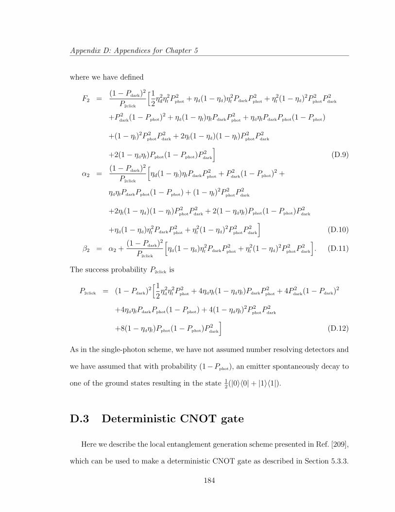
Appendix D: Appendices for Chapter 5
where we have defined
F2 =(1− Pdark)
2
P2click
[1
2η2dη
2f P
2phot + ηd(1− ηd)η
2f PdarkP
2phot + η2
f (1− ηd)2P 2
photP2dark
+P 2dark(1− Pphot)
2 + ηd(1− ηf)ηfPdarkP2phot + ηdηfPdarkPphot(1− Pphot)
+(1− ηf)2P 2
photP2dark + 2ηf(1− ηd)(1− ηf)P
2photP
2dark
+2(1− ηdηf)Pphot(1− Pphot)P2dark
](D.9)
α2 =(1− Pdark)
2
P2click
[ηd(1− ηf)ηfPdarkP
2phot + P 2
dark(1− Pphot)2 +
ηdηfPdarkPphot(1− Pphot) + (1− ηf)2P 2
photP2dark
+2ηf(1− ηd)(1− ηf)P2photP
2dark + 2(1− ηdηf)Pphot(1− Pphot)P
2dark
+ηd(1− ηd)η2f PdarkP
2phot + η2
f (1− ηd)2P 2
photP2dark
](D.10)
β2 = α2 +(1− Pdark)
2
P2click
[ηd(1− ηd)η
2f PdarkP
2phot + η2
f (1− ηd)2P 2
photP2dark
]. (D.11)
The success probability P2click is
P2click = (1− Pdark)2[1
2η2
dη2f P
2phot + 4ηdηf(1− ηdηf)PdarkP
2phot + 4P 2
dark(1− Pdark)2
+4ηdηfPdarkPphot(1− Pphot) + 4(1− ηdηf)2P 2
photP2dark
+8(1− ηdηf)Pphot(1− Pphot)P2dark
](D.12)
As in the single-photon scheme, we have not assumed number resolving detectors and
we have assumed that with probability (1−Pphot), an emitter spontaneously decay to
one of the ground states resulting in the state 12(|0〉〈0|+ |1〉〈1|).
D.3 Deterministic CNOT gate
Here we describe the local entanglement generation scheme presented in Ref. [209],
which can be used to make a deterministic CNOT gate as described in Section 5.3.3.
184
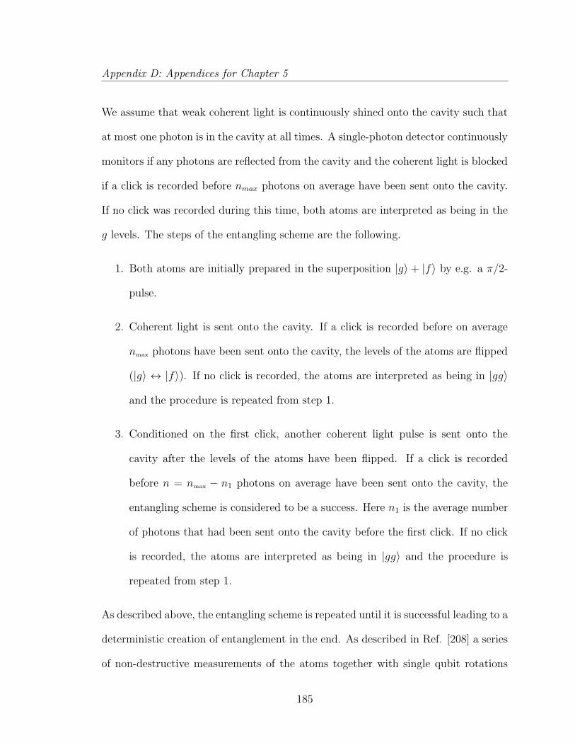
Appendix D: Appendices for Chapter 5
We assume that weak coherent light is continuously shined onto the cavity such that
at most one photon is in the cavity at all times. A single-photon detector continuously
monitors if any photons are reflected from the cavity and the coherent light is blocked
if a click is recorded before nmax photons on average have been sent onto the cavity.
If no click was recorded during this time, both atoms are interpreted as being in the
g levels. The steps of the entangling scheme are the following.
1. Both atoms are initially prepared in the superposition |g〉 + |f〉 by e.g. a π/2-
pulse.
2. Coherent light is sent onto the cavity. If a click is recorded before on average
nmax photons have been sent onto the cavity, the levels of the atoms are flipped
(|g〉 ↔ |f〉). If no click is recorded, the atoms are interpreted as being in |gg〉
and the procedure is repeated from step 1.
3. Conditioned on the first click, another coherent light pulse is sent onto the
cavity after the levels of the atoms have been flipped. If a click is recorded
before n = nmax − n1 photons on average have been sent onto the cavity, the
entangling scheme is considered to be a success. Here n1 is the average number
of photons that had been sent onto the cavity before the first click. If no click
is recorded, the atoms are interpreted as being in |gg〉 and the procedure is
repeated from step 1.
As described above, the entangling scheme is repeated until it is successful leading to a
deterministic creation of entanglement in the end. As described in Ref. [208] a series
of non-destructive measurements of the atoms together with single qubit rotations
185
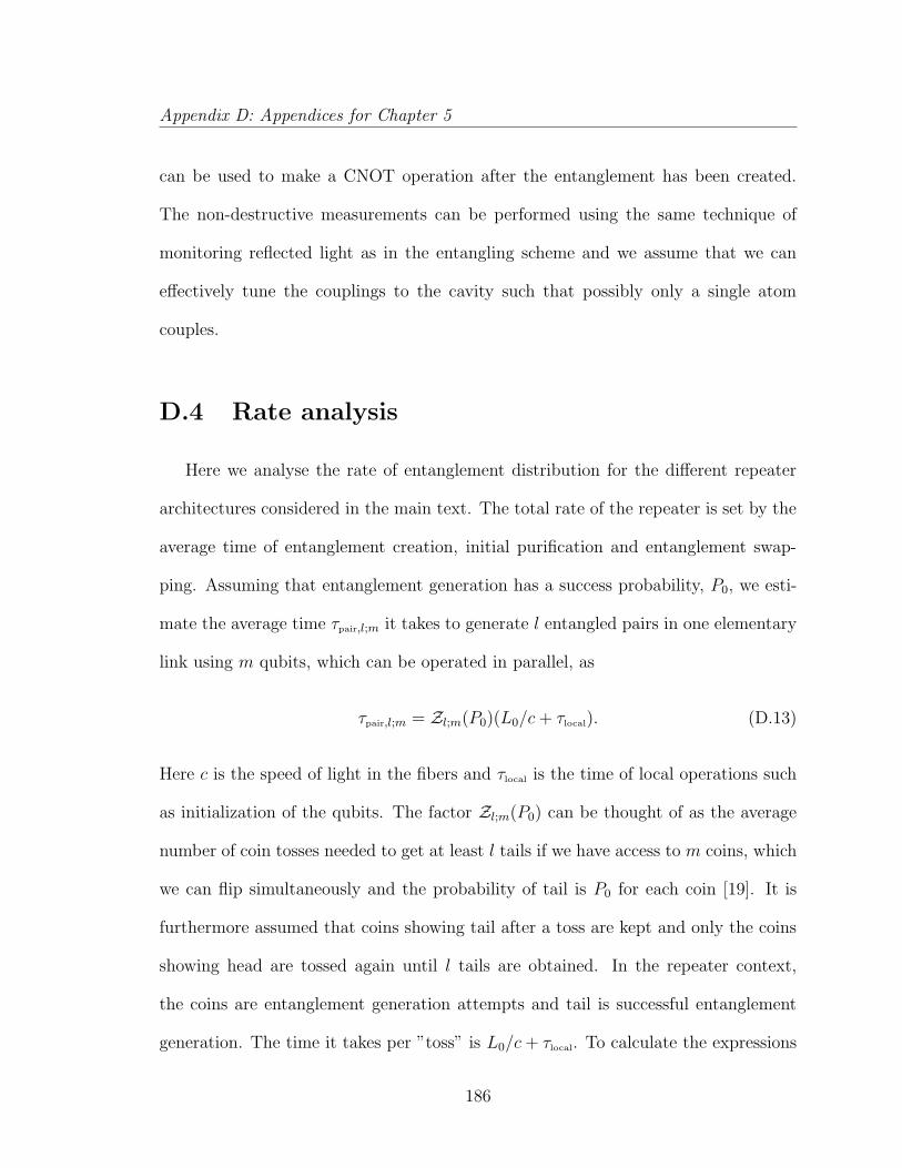
Appendix D: Appendices for Chapter 5
can be used to make a CNOT operation after the entanglement has been created.
The non-destructive measurements can be performed using the same technique of
monitoring reflected light as in the entangling scheme and we assume that we can
effectively tune the couplings to the cavity such that possibly only a single atom
couples.
D.4 Rate analysis
Here we analyse the rate of entanglement distribution for the different repeater
architectures considered in the main text. The total rate of the repeater is set by the
average time of entanglement creation, initial purification and entanglement swap-
ping. Assuming that entanglement generation has a success probability, P0, we esti-
mate the average time τpair,l;m it takes to generate l entangled pairs in one elementary
link using m qubits, which can be operated in parallel, as
τpair,l;m = Zl;m(P0)(L0/c+ τlocal). (D.13)
Here c is the speed of light in the fibers and τlocal is the time of local operations such
as initialization of the qubits. The factor Zl;m(P0) can be thought of as the average
number of coin tosses needed to get at least l tails if we have access to m coins, which
we can flip simultaneously and the probability of tail is P0 for each coin [19]. It is
furthermore assumed that coins showing tail after a toss are kept and only the coins
showing head are tossed again until l tails are obtained. In the repeater context,
the coins are entanglement generation attempts and tail is successful entanglement
generation. The time it takes per ”toss” is L0/c+ τlocal. To calculate the expressions
186
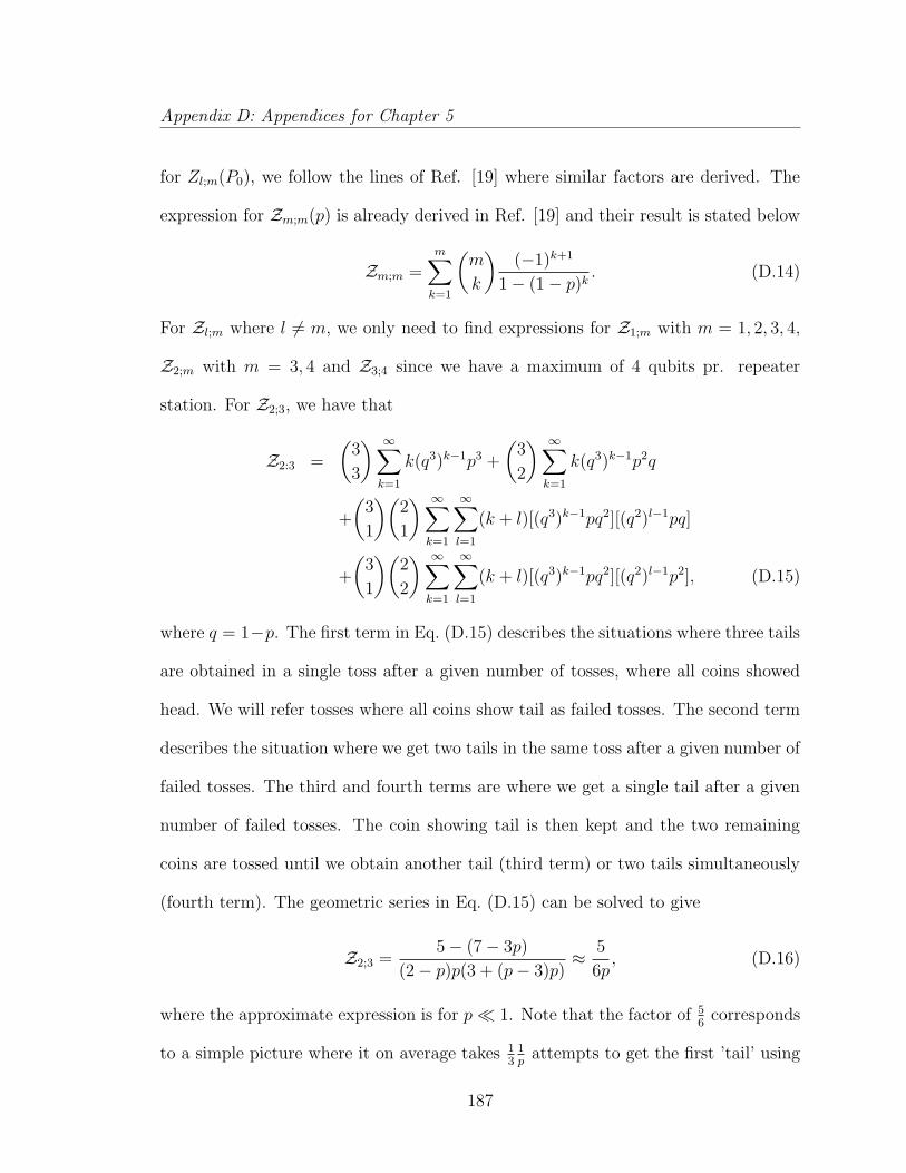
Appendix D: Appendices for Chapter 5
for Zl;m(P0), we follow the lines of Ref. [19] where similar factors are derived. The
expression for Zm;m(p) is already derived in Ref. [19] and their result is stated below
Zm;m =m∑
k=1
(m
k
)(−1)k+1
1− (1− p)k . (D.14)
For Zl;m where l 6= m, we only need to find expressions for Z1;m with m = 1, 2, 3, 4,
Z2;m with m = 3, 4 and Z3;4 since we have a maximum of 4 qubits pr. repeater
station. For Z2;3, we have that
Z2:3 =
(3
3
) ∞∑
k=1
k(q3)k−1p3 +
(3
2
) ∞∑
k=1
k(q3)k−1p2q
+
(3
1
)(2
1
) ∞∑
k=1
∞∑
l=1
(k + l)[(q3)k−1pq2][(q2)l−1pq]
+
(3
1
)(2
2
) ∞∑
k=1
∞∑
l=1
(k + l)[(q3)k−1pq2][(q2)l−1p2], (D.15)
where q = 1−p. The first term in Eq. (D.15) describes the situations where three tails
are obtained in a single toss after a given number of tosses, where all coins showed
head. We will refer tosses where all coins show tail as failed tosses. The second term
describes the situation where we get two tails in the same toss after a given number of
failed tosses. The third and fourth terms are where we get a single tail after a given
number of failed tosses. The coin showing tail is then kept and the two remaining
coins are tossed until we obtain another tail (third term) or two tails simultaneously
(fourth term). The geometric series in Eq. (D.15) can be solved to give
Z2;3 =5− (7− 3p)
(2− p)p(3 + (p− 3)p)≈ 5
6p, (D.16)
where the approximate expression is for p 1. Note that the factor of 56
corresponds
to a simple picture where it on average takes 13
1p
attempts to get the first ’tail’ using
187
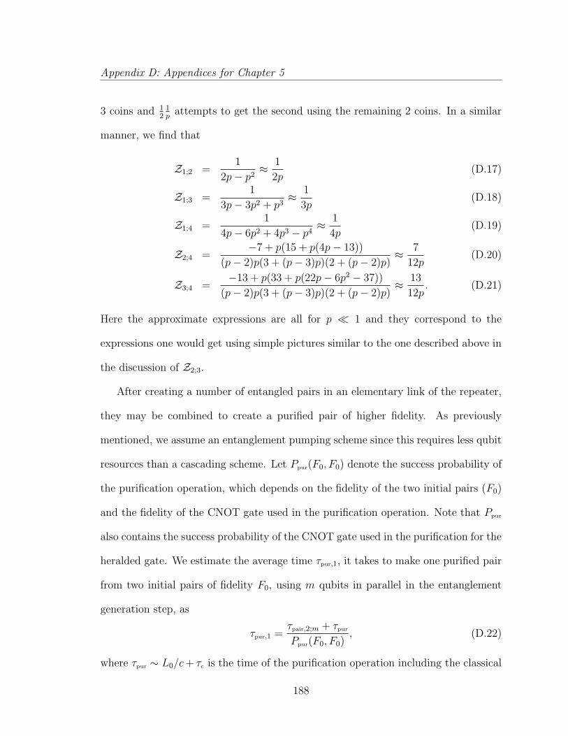
Appendix D: Appendices for Chapter 5
3 coins and 12
1p
attempts to get the second using the remaining 2 coins. In a similar
manner, we find that
Z1;2 =1
2p− p2≈ 1
2p(D.17)
Z1;3 =1
3p− 3p2 + p3≈ 1
3p(D.18)
Z1;4 =1
4p− 6p2 + 4p3 − p4≈ 1
4p(D.19)
Z2;4 =−7 + p(15 + p(4p− 13))
(p− 2)p(3 + (p− 3)p)(2 + (p− 2)p)≈ 7
12p(D.20)
Z3;4 =−13 + p(33 + p(22p− 6p2 − 37))
(p− 2)p(3 + (p− 3)p)(2 + (p− 2)p)≈ 13
12p. (D.21)
Here the approximate expressions are all for p 1 and they correspond to the
expressions one would get using simple pictures similar to the one described above in
the discussion of Z2;3.
After creating a number of entangled pairs in an elementary link of the repeater,
they may be combined to create a purified pair of higher fidelity. As previously
mentioned, we assume an entanglement pumping scheme since this requires less qubit
resources than a cascading scheme. Let Ppur(F0, F0) denote the success probability of
the purification operation, which depends on the fidelity of the two initial pairs (F0)
and the fidelity of the CNOT gate used in the purification operation. Note that Ppur
also contains the success probability of the CNOT gate used in the purification for the
heralded gate. We estimate the average time τpur,1, it takes to make one purified pair
from two initial pairs of fidelity F0, using m qubits in parallel in the entanglement
generation step, as
τpur,1 =τpair,2;m + τpur
Ppur(F0, F0), (D.22)
where τpur ∼ L0/c+ τc is the time of the purification operation including the classical
188
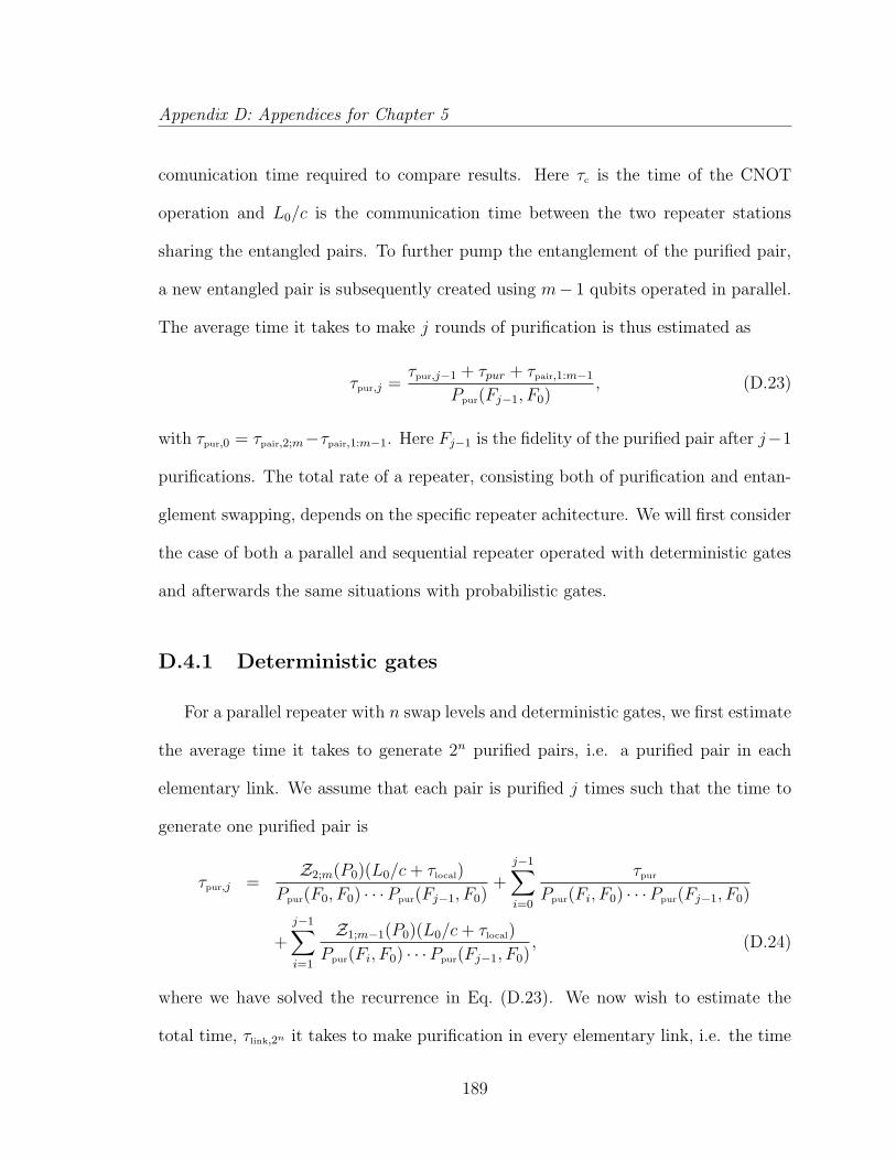
Appendix D: Appendices for Chapter 5
comunication time required to compare results. Here τc is the time of the CNOT
operation and L0/c is the communication time between the two repeater stations
sharing the entangled pairs. To further pump the entanglement of the purified pair,
a new entangled pair is subsequently created using m− 1 qubits operated in parallel.
The average time it takes to make j rounds of purification is thus estimated as
τpur,j =τpur,j−1 + τpur + τpair,1:m−1
Ppur(Fj−1, F0), (D.23)
with τpur,0 = τpair,2;m−τpair,1:m−1. Here Fj−1 is the fidelity of the purified pair after j−1
purifications. The total rate of a repeater, consisting both of purification and entan-
glement swapping, depends on the specific repeater achitecture. We will first consider
the case of both a parallel and sequential repeater operated with deterministic gates
and afterwards the same situations with probabilistic gates.
D.4.1 Deterministic gates
For a parallel repeater with n swap levels and deterministic gates, we first estimate
the average time it takes to generate 2n purified pairs, i.e. a purified pair in each
elementary link. We assume that each pair is purified j times such that the time to
generate one purified pair is
τpur,j =Z2;m(P0)(L0/c+ τlocal)
Ppur(F0, F0) · · ·Ppur(Fj−1, F0)+
j−1∑
i=0
τpur
Ppur(Fi, F0) · · ·Ppur(Fj−1, F0)
+
j−1∑
i=1
Z1;m−1(P0)(L0/c+ τlocal)
Ppur(Fi, F0) · · ·Ppur(Fj−1, F0), (D.24)
where we have solved the recurrence in Eq. (D.23). We now wish to estimate the
total time, τlink,2n it takes to make purification in every elementary link, i.e. the time
189
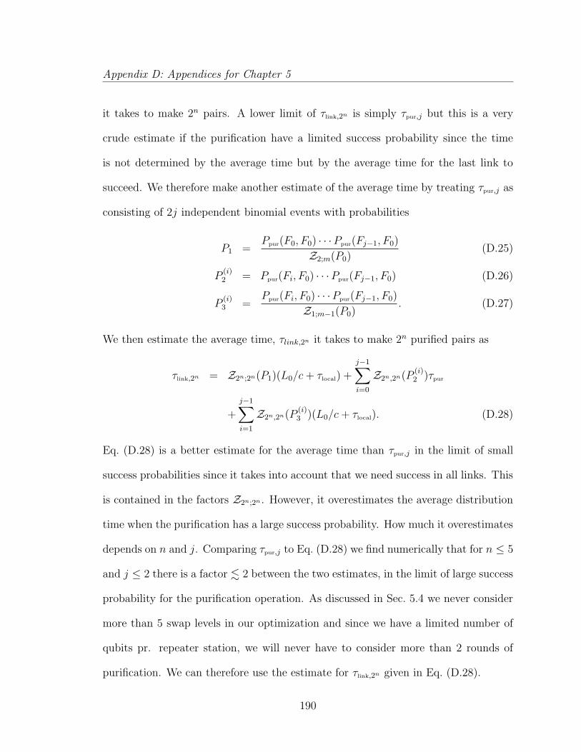
Appendix D: Appendices for Chapter 5
it takes to make 2n pairs. A lower limit of τlink,2n is simply τpur,j but this is a very
crude estimate if the purification have a limited success probability since the time
is not determined by the average time but by the average time for the last link to
succeed. We therefore make another estimate of the average time by treating τpur,j as
consisting of 2j independent binomial events with probabilities
P1 =Ppur(F0, F0) · · ·Ppur(Fj−1, F0)
Z2;m(P0)(D.25)
P(i)2 = Ppur(Fi, F0) · · ·Ppur(Fj−1, F0) (D.26)
P(i)3 =
Ppur(Fi, F0) · · ·Ppur(Fj−1, F0)
Z1;m−1(P0). (D.27)
We then estimate the average time, τlink,2n it takes to make 2n purified pairs as
τlink,2n = Z2n;2n(P1)(L0/c+ τlocal) +
j−1∑
i=0
Z2n,2n(P(i)2 )τpur
+
j−1∑
i=1
Z2n,2n(P(i)3 )(L0/c+ τlocal). (D.28)
Eq. (D.28) is a better estimate for the average time than τpur,j in the limit of small
success probabilities since it takes into account that we need success in all links. This
is contained in the factors Z2n;2n . However, it overestimates the average distribution
time when the purification has a large success probability. How much it overestimates
depends on n and j. Comparing τpur,j to Eq. (D.28) we find numerically that for n ≤ 5
and j ≤ 2 there is a factor . 2 between the two estimates, in the limit of large success
probability for the purification operation. As discussed in Sec. 5.4 we never consider
more than 5 swap levels in our optimization and since we have a limited number of
qubits pr. repeater station, we will never have to consider more than 2 rounds of
purification. We can therefore use the estimate for τlink,2n given in Eq. (D.28).
190
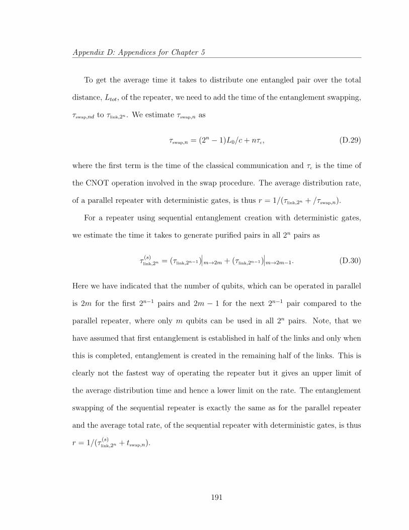
Appendix D: Appendices for Chapter 5
To get the average time it takes to distribute one entangled pair over the total
distance, Ltot, of the repeater, we need to add the time of the entanglement swapping,
τswap,nd to τlink,2n . We estimate τswap,n as
τswap,n = (2n − 1)L0/c+ nτc, (D.29)
where the first term is the time of the classical communication and τc is the time of
the CNOT operation involved in the swap procedure. The average distribution rate,
of a parallel repeater with deterministic gates, is thus r = 1/(τlink,2n + /τswap,n).
For a repeater using sequential entanglement creation with deterministic gates,
we estimate the time it takes to generate purified pairs in all 2n pairs as
τ(s)link,2n = (τlink,2n−1) m→2m + (τlink,2n−1) m→2m−1. (D.30)
Here we have indicated that the number of qubits, which can be operated in parallel
is 2m for the first 2n−1 pairs and 2m − 1 for the next 2n−1 pair compared to the
parallel repeater, where only m qubits can be used in all 2n pairs. Note, that we
have assumed that first entanglement is established in half of the links and only when
this is completed, entanglement is created in the remaining half of the links. This is
clearly not the fastest way of operating the repeater but it gives an upper limit of
the average distribution time and hence a lower limit on the rate. The entanglement
swapping of the sequential repeater is exactly the same as for the parallel repeater
and the average total rate, of the sequential repeater with deterministic gates, is thus
r = 1/(τ(s)link,2n + tswap,n).
191
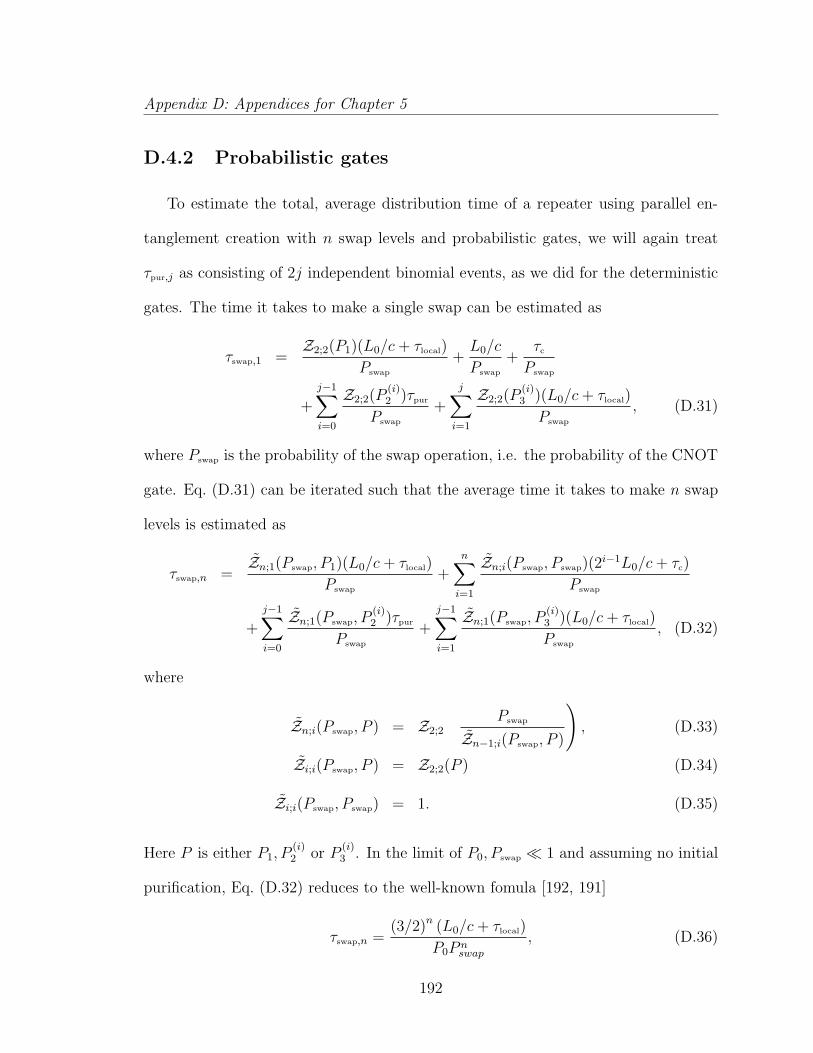
Appendix D: Appendices for Chapter 5
D.4.2 Probabilistic gates
To estimate the total, average distribution time of a repeater using parallel en-
tanglement creation with n swap levels and probabilistic gates, we will again treat
τpur,j as consisting of 2j independent binomial events, as we did for the deterministic
gates. The time it takes to make a single swap can be estimated as
τswap,1 =Z2;2(P1)(L0/c+ τlocal)
Pswap
+L0/c
Pswap
+τc
Pswap
+
j−1∑
i=0
Z2;2(P(i)2 )τpur
Pswap
+
j∑
i=1
Z2;2(P(i)3 )(L0/c+ τlocal)
Pswap
, (D.31)
where Pswap is the probability of the swap operation, i.e. the probability of the CNOT
gate. Eq. (D.31) can be iterated such that the average time it takes to make n swap
levels is estimated as
τswap,n =Zn;1(Pswap, P1)(L0/c+ τlocal)
Pswap
+n∑
i=1
Zn;i(Pswap, Pswap)(2i−1L0/c+ τc)
Pswap
+
j−1∑
i=0
Zn;1(Pswap, P(i)2 )τpur
Pswap
+
j−1∑
i=1
Zn;1(Pswap, P(i)3 )(L0/c+ τlocal)
Pswap
, (D.32)
where
Zn;i(Pswap, P ) = Z2;2
(Pswap
Zn−1;i(Pswap, P )
), (D.33)
Zi;i(Pswap, P ) = Z2;2(P ) (D.34)
Zi;i(Pswap, Pswap) = 1. (D.35)
Here P is either P1, P(i)2 or P
(i)3 . In the limit of P0, Pswap 1 and assuming no initial
purification, Eq. (D.32) reduces to the well-known fomula [192, 191]
τswap,n =(3/2)n (L0/c+ τlocal)
P0P nswap
, (D.36)
192
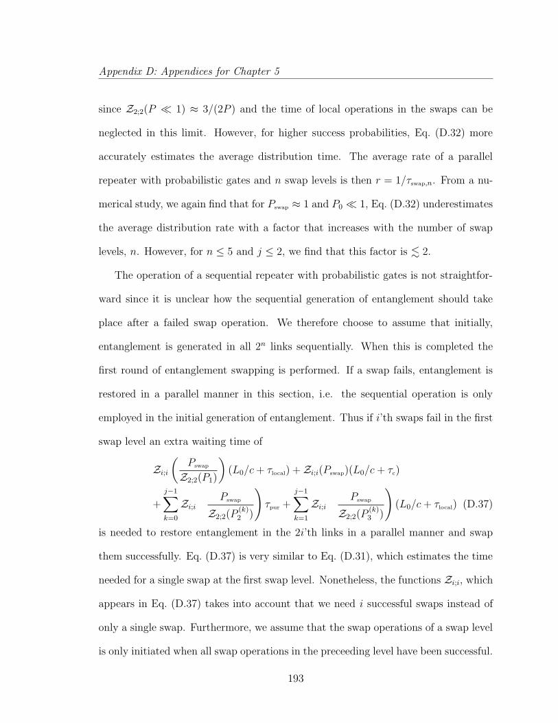
Appendix D: Appendices for Chapter 5
since Z2;2(P 1) ≈ 3/(2P ) and the time of local operations in the swaps can be
neglected in this limit. However, for higher success probabilities, Eq. (D.32) more
accurately estimates the average distribution time. The average rate of a parallel
repeater with probabilistic gates and n swap levels is then r = 1/τswap,n. From a nu-
merical study, we again find that for Pswap ≈ 1 and P0 1, Eq. (D.32) underestimates
the average distribution rate with a factor that increases with the number of swap
levels, n. However, for n ≤ 5 and j ≤ 2, we find that this factor is . 2.
The operation of a sequential repeater with probabilistic gates is not straightfor-
ward since it is unclear how the sequential generation of entanglement should take
place after a failed swap operation. We therefore choose to assume that initially,
entanglement is generated in all 2n links sequentially. When this is completed the
first round of entanglement swapping is performed. If a swap fails, entanglement is
restored in a parallel manner in this section, i.e. the sequential operation is only
employed in the initial generation of entanglement. Thus if i’th swaps fail in the first
swap level an extra waiting time of
Zi;i(
Pswap
Z2;2(P1)
)(L0/c+ τlocal) + Zi;i(Pswap)(L0/c+ τc)
+
j−1∑
k=0
Zi;i(
Pswap
Z2;2(P(k)2 )
)τpur +
j−1∑
k=1
Zi;i(
Pswap
Z2;2(P(k)3 )
)(L0/c+ τlocal) (D.37)
is needed to restore entanglement in the 2i’th links in a parallel manner and swap
them successfully. Eq. (D.37) is very similar to Eq. (D.31), which estimates the time
needed for a single swap at the first swap level. Nonetheless, the functions Zi;i, which
appears in Eq. (D.37) takes into account that we need i successful swaps instead of
only a single swap. Furthermore, we assume that the swap operations of a swap level
is only initiated when all swap operations in the preceeding level have been successful.
193
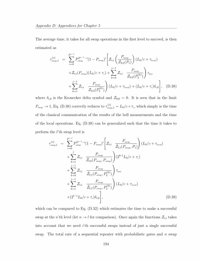
Appendix D: Appendices for Chapter 5
The average time, it takes for all swap operations in the first level to succeed, is then
estimated as
τ(s)swap,1 =
2n−1∑
i=0
P 2n−1−iswap (1− Pswap)
i
[Zi;i
(Pswap
Z2;2(P1)
)(L0/c+ τlocal)
+Zi;i(Pswap)(L0/c+ τc) +
j−1∑
k=0
Zi;i(
Pswap
Z2;2(P(k)2 )
)τpur
+
j−1∑
k=1
Zi;i(
Pswap
Z2;2(P(k)3 )
)(L0/c+ τlocal) + (L0/c+ τc)δi,0
], (D.38)
where δi,0 is the Kronecker delta symbol and Z0;0 = 0. It is seen that in the limit
Pswap → 1, Eq. (D.38) correctly reduces to τ(s)swap,1 = L0/c+τc, which simply is the time
of the classical communication of the results of the bell measurements and the time
of the local operations. Eq. (D.38) can be generalized such that the time it takes to
perform the l’th swap level is
τ(s)swap,l =
2n−l∑
i=0
P 2n−l−iswap (1− Pswap)
i
[Zi;i
(Pswap
Zl;1(Pswap, P1)
)(L0/c+ τlocal)
+l∑
k=1
Zi;i(
Pswap
Zl;k(Pswap, Pswap)
)(2k−1L0/c+ τc)
+
j−1∑
k=0
Zi;i(
Pswap
Zl;1(Pswap, P(k)2 )
)τpur
+
j−1∑
k=1
Zi;i(
Pswap
Zl;1(Pswap, P(k)3 )
)(L0/c+ τlocal)
+(2l−1L0/c+ τc)δi,0
], (D.39)
which can be compared to Eq. (D.32) which estimates the time to make a successful
swap at the n’th level (let n→ l for comparison). Once again the functions Zi;i takes
into account that we need i’th successful swaps instead of just a single successful
swap. The total rate of a sequential repeater with probabilistic gates and n swap
194
Appendix D: Appendices for Chapter 5
levels can then be estimated as r = 1/(τ(s)link,2n + τ
(s)swap,1 + · · ·+ τ
(s)swap,n).
195
Appendix E
Appendices for Chapter 6
E.1 Figure of merit: Allan-variance
ProvidedN qubits, we aim to devise an efficient interrogation scheme that provides
input for the feedback mechanism, using Ramsey spectroscopy. After the kth Ramsey
cycle, of length T , an estimate ΦestLO(tk) is obtained for the accumulated phase of the
LO, ΦLO(tk) =∫ tktk−T
dt δω(t), (tk = kT , k = 1, 2 . . . , and δω(t) = ω(t) − ω0), which
differs from the real value by ∆ΦLO(tk) = ΦestLO(tk) − Φreal
LO (tk). Using the obtained
estimate, the feedback mechanism corrects the phase or frequency of the LO after
every cycle, and thus creates a LO signal with better stability. The figure of merit
for stability is the Allan-variance, σ2y(τ) = 1
ω20〈δω2(t0)〉t0 where δω(t0) denotes the
time-average of δω(t0 + t) over t ∈ [0, τ ], where τ is the available averaging time, 〈 〉t0stands for time-average over t0, which is much longer than τ , ω0 is the frequency of
the chosen clock transition. Consequently, one readily shows that the Allan variance
196
Appendix E: Appendices for Chapter 6
can be written as,
σ2y(τ) =
1
ω20τ
2
τ/T∑
i=1
τ/T∑
j=1
⟨∆ΦLO(t0 + iT )∆ΦLO(t0 + jT )
⟩t0. (E.1)
By assuming that ∆ΦLO is a stationary random process, we substitute the average
over t0 with the average over many realizations. With the notation ∆ΦLO(t0 + jT ) =
∆ΦLO,j, we can write this average as
〈∆ΦLO,i∆ΦLO,j〉 ≈⟨∆Φ2
LO
⟩δij, (E.2)
where we further used a white noise assumption, such that phase accumulations in
consecutive Ramsey cycle are approximately uncorrelated. Also for realistic 1/f laser
noise spectra, numerical studies show that this factorization assumption leads to only
negligible corrections. Earlier results show that this is the case for initial LO frequency
noise spectra, Sν(f) that are less divergent than 1/f 2 at low frequencies [7]. As a
result, the Allan-variance simplifies to,
σ2y(τ) =
1
ω20τT
⟨∆Φ2
LO
⟩, (E.3)
linking the achieving stability directly to the frequency measurement uncertainty
during the interrogation. Eq. E.3 serves as our starting point in finding the optimal
measurement protocol that minimizes σ2y(τ) for fixed N and τ . In the following,
we investigate and compare different classical and quantum mechanical strategies
for the interrogation of the (from cycle to cycle fluctuating) quantity ΦLO, and we
demonstrate that the proposed interrogation protocol using cascaded GHZ states is
optimal up to a logarithmic correction.
197
Appendix E: Appendices for Chapter 6
E.2 Single-step Uncorrelated ensemble
First, we consider the case of naive interrogation using a Ramsey protocol with
N uncorrelated atoms.
E.2.1 Sub-ensembles and projection noise
Single ensemble Ramsey spectroscopy is limited to estimating either the real or
the imaginary part of eiΦLO . However, by dividing the available qubits into two sub-
ensembles, X and Y , preparing their individual qubits in different states,
X : [|0〉+ |1〉]/√
2, (E.4)
Y : [|0〉+ i|1〉]/√
2, (E.5)
and performing the same Ramsey measurement on them, we can get estimates on
both the real and imaginary parts of eiΦLO and deduce the value of ΦLO up to 2π
shifts, instead of π. At the end of the free evolution time, each qubit in ensemble X
(Y ) is measured in the x-basis (|±〉 = [|0〉± |1〉]/√
2) and yields the ’+’ outcome with
probability px = [1− cos ΦLO]/2 (py = [1− sin ΦLO]/2).
After performing the measurement with N total qubits, we obtain ΦestLO from the
estimates of px and py. Since both provide information on ΦestLO equivalent of N/2
measurement bits, this results in a total information of N measurement bits, which
gives an uncertainty of
⟨∆Φ2
LO
⟩pr
=1
N, (E.6)
up to 2π phase shifts, that are fundamentally undetectable. This method is identical
to the one described in [183].
198
Appendix E: Appendices for Chapter 6
E.2.2 Effects of laser fluctuations: Phase slip errors
Random fluctuations in the laser frequency (characterized by the laser spectrum
noise spectrum Sν(f) = 2γLO/f) result in the fact that the laser phase itself has to
be considered as a random variable after each cycle. Whenever in a given cycle the
phase ΦLO(tk) falls outside the interval [−π, π], the aforementioned technique leads
to an estimate deviating from the true value by ∼ 2π. As the variance s2 of the
prior distribution of ΦLO grows with the interrogation time T (one finds s2 = γLOT
(s2 = (γLOT )2) for a white (1/f) noise frequency spectrum, where γLO denotes the
laser linewidth of the free-running (non-stabilized) LO) these undetected phase slips
pose a fundamental limitation on the allowed Ramsey time T , and thus on the overall
achievable laser stability.
If we assume a constant rate of phase diffusion, resulting in a Gaussian prior
distribution of ΦLO, the probability of a phase slip single cycle of length T can be
estimated as
Pslip = 2
∞∫
π
dΦrealLO
1√2πs2
exp
[−(Φreal
LO )2
2s2
](E.7)
= 1− erf
(π√2s
)=
(√2s
π3/2+O(s2)
)exp
[− π2
2s2
], (E.8)
where erf denotes the error function. As a phase slip in an early Ramsey cycle will
remain undetected in the following cycles, its error contribution will accumulate over
the total averaging time τ , in the worst case by a factor τ/T . Using this upper bound,
and assuming Pslip 1 we write the variance contribution of phase slips as
⟨∆Φ2
LO
⟩slip
= (2π)2 τ
TPslip ≈ (2π)2 τ
T
√2
π3/2
√γLOT exp
[− π2
2γLOT
], (E.9)
199
Appendix E: Appendices for Chapter 6
where the (2π)2 prefactor sets the absolute contribution of a manifested slip event
to ±2π, and in the second step we approximated Pslip with the first term of its
asymptotic series from Eq. E.8.
E.2.3 Optimal Ramsey time
While (E.3) suggests increasing Ramsey times improve the laser stability, we have
seen in the previous section that they also lead to an increased occurrence of phase
slips yielding a significant contribution to the measurement uncertainty.
In order to find the optimal Ramsey time we add the contributions from quantum
projection noise [Eq. E.6] and phase slip noise [Eq. E.9] under the assumption that
the probability of phase slips is small, and obtain an expression for the Allan-variance,
σ2y(τ) =
1
ω20τ
Γ, (E.10)
where
Γ =1
TN+√
32πτγ
1/2LO
T 3/2exp
[− π2
2γLOT
]. (E.11)
In order to find the optimal Ramsey time Topt, that minimizes Γ, we introduce the
new variable x = 2π2γLOT , and write
Γ =2
π2
γLO
Nx+
16
π5/2
τγ2LO
x3/2e−1/x. (E.12)
Taking the derivative with respect to x results in
d
dxΓ = − 2
π2
γLO
Nx2+
16
π5/2τγ2
LO
(−3
2
1
x3/2+
1
x7/2
)e−1/x, (E.13)
which, after using the (self-consistent) assumption xopt 1, results in the following
transcendental equation for xopt,
x3/2opt = ((8/
√π)γLOτN)e−1/xopt . (E.14)
200

Appendix E: Appendices for Chapter 6
In Section E.4, we provide the derivation of the asymptotic solution,
xopt = [log((8/√π)γLOτN)]−1 ≈ [log(γLOτN)]−1, (E.15)
yielding directly
Topt ≈ γ−1LO
π2
2[log(γLOτN)]−1. (E.16)
Self-consistently we confirm that already for values γLOτN ≥ 104, the approximation
in Eq. E.9 is well justified, so that the above value represents a true local minimum.
For larger values of T the phase slip errors grow rapidly, and numerical studies confirm
that Eq. E.16 indeed represents a global minimum.
The optimal interrogation time is mainly set by the LO coherence time γ−1LO, and
shows a weak dependence on the total number of qubits N , and the averaging time
τ (Note, that if we model the LO with a 1/f frequency noise spectrum, only the
exponent of the log term changes to −1/2 in this result). Using this optimized
Ramsey time we find for the minimal value of Γ is
Γmin =2
π2
γLO
Nxopt
+16
π5/2
τγ2LO
x3/2opt
e−1/xopt (E.17)
=2
π2
γLO
N
(1
xopt
+ 1
)(E.18)
≈ 2
π2
γLO log(γLOτN)
N. (E.19)
This result is valid as long as the averaging time τ is longer than the proposed
Topt from Eq. E.16. If this is not the case, then Topt = τ , the phase slip noise becomes
negligible, and we end up with
Γmin =1
τN. (E.20)
201
Appendix E: Appendices for Chapter 6
We approximate the crossover region (around τ ∼ γ−1LO) by adding leading terms
from Eq. E.19 & (E.20) and obtain
[σy(τ)]min ≈1
ω0
√Nτ
√1
τ+
2
π2γLO log(γLOτN). (E.21)
In summary, in the region τ < Topt, the LO noise is negligible leading to a linear
scaling of the ADEV with the total averaging time τ . For large averaging times
τ > Topt, phase slips of the laser phase pose a limitation to the maximal possible
Ramsey time which results in a 1/√τ scaling of the laser stability. Since we employ
uncorrelated atoms, the ADEV displays in both regimes the 1/√N scaling of the
standard quantum limit (SQL). As modern atomic clocks typically are laser noise
limited, γLO γind (where γind represents the clock atom linewidth), we neglected
the effects of individual atomic dephasing in the above considerations.
E.3 Cascaded interrogation using GHZ states
In this Section, we discuss the possibility of using quantum correlated states,
namely GHZ states of the form
[|0〉+ eiχ|1〉]/√
2, (E.22)
where |0〉 and |1〉 are product states of all qubits being in |0〉 or |1〉, respectively, and
χ will be referred to as the phase of the GHZ state. Such a state, once prepared,
is more sensitive to the accumulated phase of the LO, ΦLO, by a factor of N ′, the
number of qubits entangled:(
N∏
j=1
Uj
)[|0〉+ eiχ|1〉
]/√
2 = [|0〉+ ei(χ+N ′ΦLO)|1〉]/√
2, (E.23)
202
Appendix E: Appendices for Chapter 6
where Uj = |0〉〈0|+ eiΦLO |1〉〈1| is the time propagation operator for the interrogation
time acting on the jth qubit. This property promises an enhancement in phase
resolution, and therefore a better stability for quantum clocks.
E.3.1 Parity measurement
Using the idea with the two sub-ensembles [see Eq. E.4 and (E.5)], we imagine
dividing the qubits into two equal groups, and preparing two separate GHZ states:
|X〉 := [|0〉+ |1〉]/√
2, (E.24)
|Y 〉 := [|0〉+ i|1〉]/√
2, (E.25)
each entangling N ′ qubits. After the free evolution time, we imagine measuring each
qubits in the x-basis (|±〉 = [|0〉∓ |1〉]/√
2) separately. In this basis, the above states
are written as
[( |+〉 − |−〉√2
)⊗N ′+ eiφν
( |+〉+ |−〉√2
)⊗N ′]/√
2, (E.26)
where φν = χν + N ′ΦLO, for ν ∈ x, y and χx = 0, while χy = π/2 for the two
groups, respectively. The above state can be written as
1
2(N ′+1)/2
∑
q∈+,−×N′
[(N ′∏
j=1
qj
)+ eiφν
]|q1, q2, . . . qN ′〉. (E.27)
Once the qubits are measured one by one, the probability to measure a certain out-
come q = (q1, q2, . . . qN ′), (qj ∈ +,−) is
P(q) =1
2N ′+1|1 + p(q)eiφν |2, (E.28)
203
Appendix E: Appendices for Chapter 6
where p(q) =∏N ′
j=1 qj is the parity of the sum of all measurement bits. This parity is
the observable that is sensitive to the accumulated phase, since its distribution is
P(p = ±1) =1± cos(φν)
2. (E.29)
This is identical to the parity measurement scheme described in [24]. By interro-
gating n0/2 instances of |X〉 and |Y 〉, respectively, we can measure the phase of the
GHZ state, N ′ΦLO, with uncertainty 1/√n0, since each instance provides a single
measurement bit, which can be combined the same way as we described in the case
of uncorrelated ensembles. The resulting measurement uncertainty, ∆ΦLO, is
⟨∆Φ2
LO
⟩pr
=1
(N ′)2n0
=n0
N2, (E.30)
which is a factor of N/n0 smaller than the variance contribution of projection noise
for the uncorrelated ensemble protocol, (N = n0N′).
E.3.2 Failure of the maximally entangled GHZ
Motivated by the increased phase resolution provided by the interrogation of GHZ
states, we evaluate the stability of such a protocol. We find that it fails to provide
improvement compared to the single-step uncorrelated protocol due to an increased
phase slip rate. This is in agreement with earlier results [237, 184].
The probability, that the phase accumulated by |X〉 (|Y 〉) during the interrogation
time T , N ′ΦLO lies outside the interval [−π, π], is
Pslip = 2
∞∫
π/N ′
dΦrealLO
1√2πγLOT
exp
[−(Φreal
LO )2
2γLOT
], (E.31)
204

Appendix E: Appendices for Chapter 6
which, due to the much lower slipping threshold of π/N ′ [instead of π in the uncorre-
lated case, compare Eq. E.7] will become significant for much shorter T cycle times.
The resulting variance contribution (following the same argument as before) is
⟨∆Φ2
LO
⟩slip
=√
32πτ
T
√γLOTN
′ exp
[− π2
2γLOT (N ′)2
]. (E.32)
Neglecting the individual qubit noise by the same argument as before, we simply add
the contributions from Eq. E.30 and Eq. E.32 to obtain the Allan-variance, σ2y(τ) =
1ω2
0τΓ, where
Γ =1
NN ′T+√
32πτγ
1/2LO
T 3/2N ′ exp
[− π2
2γLOT (N ′)2
]. (E.33)
After optimizing T , we find
Topt ≈π2
2
1
γLO(N ′)2
1
log[γLOτN(N ′)3], (E.34)
which results in the minimal Allan-variance,
[σy(τ)]min ≈1
ω0
√2
π
√γLON ′ log[γLOτN(N ′)3]
τN, (E.35)
which is at least a factor of√N ′ bigger than the smallest obtainable Allan-variance
with the single-step uncorrelated protocol [Eq. E.19]. In case of a 1/f LO frequency
noise spectrum, Topt ∝ 1N
(up to logarithmic terms), and the resulting Allan-variance
is equal to Eq. E.19, up to logarithmic corrections, yielding effectively no advantage
over the uncorrelated scheme.
E.3.3 Cascaded GHZ scheme
As demonstrated in the previous Section, single GHZ states fail to improve clock
stability because the increase in sensitivity to the laser detuning, at the same time,
205
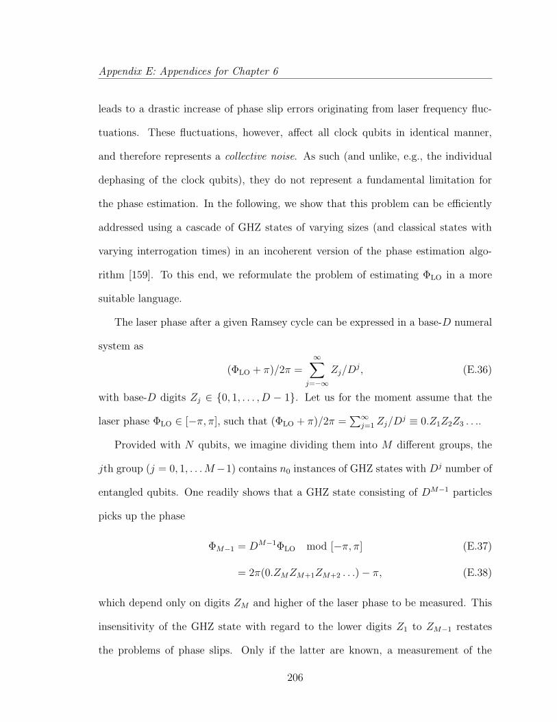
Appendix E: Appendices for Chapter 6
leads to a drastic increase of phase slip errors originating from laser frequency fluc-
tuations. These fluctuations, however, affect all clock qubits in identical manner,
and therefore represents a collective noise. As such (and unlike, e.g., the individual
dephasing of the clock qubits), they do not represent a fundamental limitation for
the phase estimation. In the following, we show that this problem can be efficiently
addressed using a cascade of GHZ states of varying sizes (and classical states with
varying interrogation times) in an incoherent version of the phase estimation algo-
rithm [159]. To this end, we reformulate the problem of estimating ΦLO in a more
suitable language.
The laser phase after a given Ramsey cycle can be expressed in a base-D numeral
system as
(ΦLO + π)/2π =∞∑
j=−∞
Zj/Dj, (E.36)
with base-D digits Zj ∈ 0, 1, . . . , D − 1. Let us for the moment assume that the
laser phase ΦLO ∈ [−π, π], such that (ΦLO + π)/2π =∑∞
j=1 Zj/Dj ≡ 0.Z1Z2Z3 . . ..
Provided with N qubits, we imagine dividing them into M different groups, the
jth group (j = 0, 1, . . .M−1) contains n0 instances of GHZ states with Dj number of
entangled qubits. One readily shows that a GHZ state consisting of DM−1 particles
picks up the phase
ΦM−1 = DM−1ΦLO mod [−π, π] (E.37)
= 2π(0.ZMZM+1ZM+2 . . .)− π, (E.38)
which depend only on digits ZM and higher of the laser phase to be measured. This
insensitivity of the GHZ state with regard to the lower digits Z1 to ZM−1 restates
the problems of phase slips. Only if the latter are known, a measurement of the
206
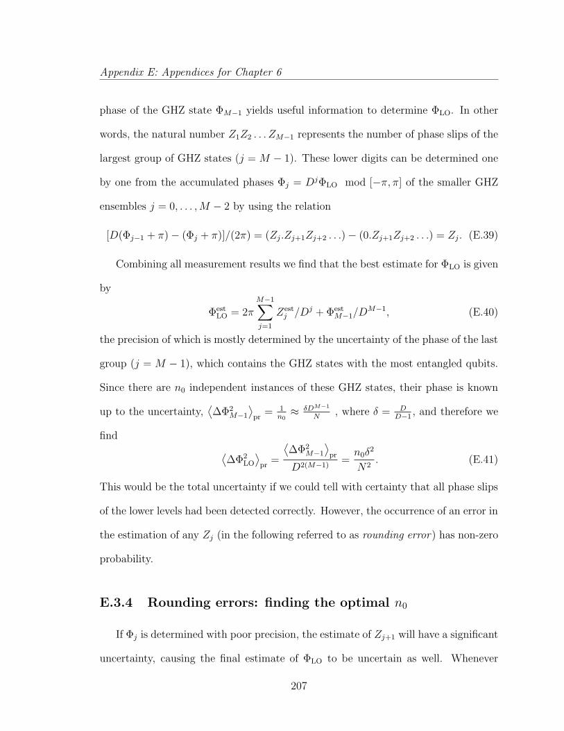
Appendix E: Appendices for Chapter 6
phase of the GHZ state ΦM−1 yields useful information to determine ΦLO. In other
words, the natural number Z1Z2 . . . ZM−1 represents the number of phase slips of the
largest group of GHZ states (j = M − 1). These lower digits can be determined one
by one from the accumulated phases Φj = DjΦLO mod [−π, π] of the smaller GHZ
ensembles j = 0, . . . ,M − 2 by using the relation
[D(Φj−1 + π)− (Φj + π)]/(2π) = (Zj.Zj+1Zj+2 . . .)− (0.Zj+1Zj+2 . . .) = Zj. (E.39)
Combining all measurement results we find that the best estimate for ΦLO is given
by
ΦestLO = 2π
M−1∑
j=1
Zestj /Dj + Φest
M−1/DM−1, (E.40)
the precision of which is mostly determined by the uncertainty of the phase of the last
group (j = M − 1), which contains the GHZ states with the most entangled qubits.
Since there are n0 independent instances of these GHZ states, their phase is known
up to the uncertainty,⟨∆Φ2
M−1
⟩pr
= 1n0≈ δDM−1
N, where δ = D
D−1, and therefore we
find
⟨∆Φ2
LO
⟩pr
=
⟨∆Φ2
M−1
⟩pr
D2(M−1)=n0δ
2
N2. (E.41)
This would be the total uncertainty if we could tell with certainty that all phase slips
of the lower levels had been detected correctly. However, the occurrence of an error in
the estimation of any Zj (in the following referred to as rounding error) has non-zero
probability.
E.3.4 Rounding errors: finding the optimal n0
If Φj is determined with poor precision, the estimate of Zj+1 will have a significant
uncertainty, causing the final estimate of ΦLO to be uncertain as well. Whenever
207

Appendix E: Appendices for Chapter 6
|Φestj − Φreal
j | > π/D, we make a mistake by under- or overestimating the digit Zj+1.
To minimize the effect of this error, we need to optimize how the qubits are distributed
on various levels of the cascade. In other words, for a given total particle number N
and basis D we need to find the optimal value of n0, the number of copies of GHZ
states in each step 1.
The probability that a rounding error occurs during the estimation of Zj is
Pre = 2
∞∫
π/D
dφ ρ(φ− Φrealj ) ≤ 2
∞∫
π/D
dφn3/20 exp
[−n0φ
2
2
]
≈ 2
πn
1/20 D exp
[−n0π
2
2D2
], (E.42)
where φ = Φestj−1 − Φreal
j−1, and ρ is the conditional distribution of Φestj−1 for given
Φrealj−1. The employed upper bound is obtained in section E.5, with the assumption
γLO/γind N/n0 (γind is the individual qubit dephasing rate), so that the projection
noise is the dominant noise term. Due to the fixed value of n0 accross different levels
of the cascade, this probability is independent of j, however the phase shift imposed
on ΦLO by a manifested rounding error of Zj is 2πD−j (j = 1, . . .M −1), as rounding
errors early in the cascade are more harmful than later ones. This results in the total
variance contribution,
⟨∆Φ2
LO
⟩re
= Pre
M−1∑
j=1
(2πD−j)2 ≈ 8π
√N
δD−
M−32 exp
[−n0π
2
2D2
]1
D2 − 1. (E.43)
By adding the two error contributions from Eq. F.11 and Eq. F.17, we obtain
the total uncertainty, 〈∆Φ2LO〉 and the corresponding Allan-variance [according to
1In principle, the clock stability can further be improved by employing different numbers of copiesin each step of the Cascade. However, this possibility will not be pursuit in this work.
208
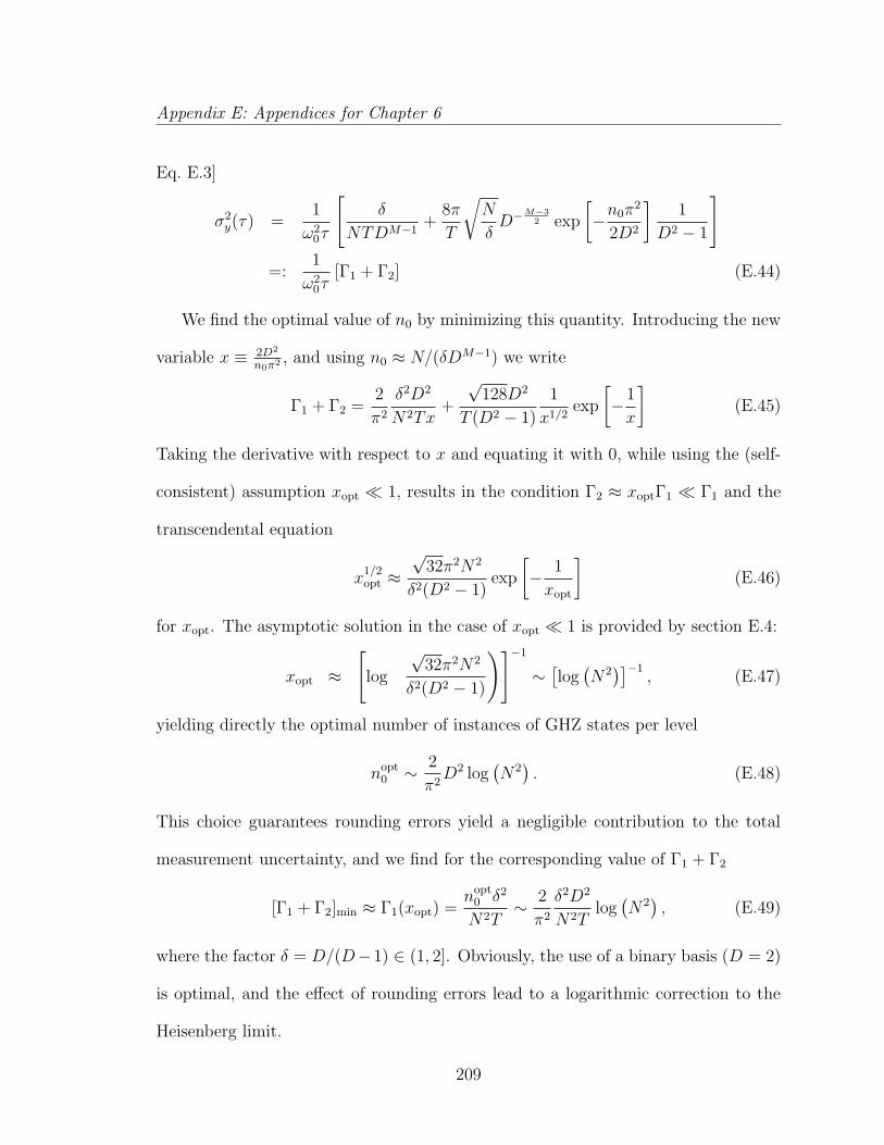
Appendix E: Appendices for Chapter 6
Eq. E.3]
σ2y(τ) =
1
ω20τ
[δ
NTDM−1+
8π
T
√N
δD−
M−32 exp
[−n0π
2
2D2
]1
D2 − 1
]
=:1
ω20τ
[Γ1 + Γ2] (E.44)
We find the optimal value of n0 by minimizing this quantity. Introducing the new
variable x ≡ 2D2
n0π2 , and using n0 ≈ N/(δDM−1) we write
Γ1 + Γ2 =2
π2
δ2D2
N2Tx+
√128D2
T (D2 − 1)
1
x1/2exp
[−1
x
](E.45)
Taking the derivative with respect to x and equating it with 0, while using the (self-
consistent) assumption xopt 1, results in the condition Γ2 ≈ xoptΓ1 Γ1 and the
transcendental equation
x1/2opt ≈
√32π2N2
δ2(D2 − 1)exp
[− 1
xopt
](E.46)
for xopt. The asymptotic solution in the case of xopt 1 is provided by section E.4:
xopt ≈[
log
( √32π2N2
δ2(D2 − 1)
)]−1
∼[log(N2)]−1
, (E.47)
yielding directly the optimal number of instances of GHZ states per level
nopt0 ∼ 2
π2D2 log
(N2). (E.48)
This choice guarantees rounding errors yield a negligible contribution to the total
measurement uncertainty, and we find for the corresponding value of Γ1 + Γ2
[Γ1 + Γ2]min ≈ Γ1(xopt) =nopt
0 δ2
N2T∼ 2
π2
δ2D2
N2Tlog(N2), (E.49)
where the factor δ = D/(D−1) ∈ (1, 2]. Obviously, the use of a binary basis (D = 2)
is optimal, and the effect of rounding errors lead to a logarithmic correction to the
Heisenberg limit.
209
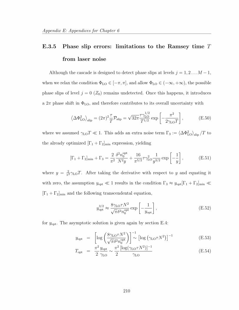
Appendix E: Appendices for Chapter 6
E.3.5 Phase slip errors: limitations to the Ramsey time T
from laser noise
Although the cascade is designed to detect phase slips at levels j = 1, 2 . . .M − 1,
when we relax the condition ΦLO ∈ [−π, π], and allow ΦLO ∈ (−∞,+∞), the possible
phase slips of level j = 0 (Z0) remains undetected. Once this happens, it introduces
a 2π phase shift in ΦLO, and therefore contributes to its overall uncertainty with
⟨∆Φ2
LO
⟩slip
= (2π)2 τ
TPslip =
√32π
τγ1/2LO
T 1/2exp
[− π2
2γLOT
], (E.50)
where we assumed γLOT 1. This adds an extra noise term Γ3 := 〈∆Φ2LO〉slip /T to
the already optimized [Γ1 + Γ2]min expression, yielding
[Γ1 + Γ2]min + Γ3 =2
π2
δ2nopt0
N2y+
16
π5/2τγ2
LO
1
y3/2exp
[−1
y
], (E.51)
where y = 2π2γLOT . After taking the derivative with respect to y and equating it
with zero, the assumption yopt 1 results in the condition Γ3 ≈ yopt[Γ1 + Γ2]min
[Γ1 + Γ2]min and the following transcendental equation,
y3/2opt ≈
8γLOτN2
√πδ2nopt
0
exp
[− 1
yopt
], (E.52)
for yopt. The asymptotic solution is given again by section E.4:
yopt =
[log
(8γLOτN
2
√πδ2nopt
0
)]−1
∼[log(γLOτN
2)]−1
(E.53)
Topt =π2
2
yopt
γLO
∼ π2
2
[log(γLOτN2)]−1
γLO
(E.54)
210
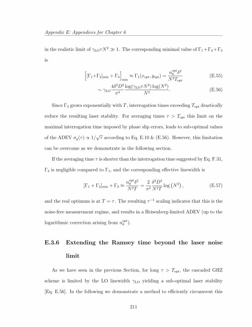
Appendix E: Appendices for Chapter 6
in the realistic limit of γLOτN2 1. The corresponding minimal value of Γ1 +Γ2 +Γ3
is
[[Γ1+Γ2]min + Γ3
]min≈ Γ1(xopt, yopt) =
nopt0 δ2
N2Topt
(E.55)
∼ γLO4δ2D2
π4
log(γLOτN2) log(N2)
N2. (E.56)
Since Γ3 grows exponentially with T , interrogation times exceeding Topt drastically
reduce the resulting laser stability. For averaging times τ > Topt this limit on the
maximal interrogation time imposed by phase slip errors, leads to sub-optimal values
of the ADEV σy(τ) ∝ 1/√τ according to Eq. E.10 & (E.56). However, this limitation
can be overcome as we demonstrate in the following section.
If the averaging time τ is shorter than the interrogation time suggested by Eq. F.31,
Γ3 is negligible compared to Γ1, and the corresponding effective linewidth is
[Γ1 + Γ2]min + Γ3 ≈nopt
0 δ2
N2T=
2
π2
δ2D2
N2Tlog(N2), (E.57)
and the real optimum is at T = τ . The resulting τ−1 scaling indicates that this is the
noise-free measurement regime, and results in a Heisenberg-limited ADEV (up to the
logarithmic correction arising from nopt0 ).
E.3.6 Extending the Ramsey time beyond the laser noise
limit
As we have seen in the previous Section, for long τ > Topt, the cascaded GHZ
scheme is limited by the LO linewidth γLO yielding a sub-optimal laser stability
[Eq. E.56]. In the following we demonstrate a method to efficiently circumvent this
211
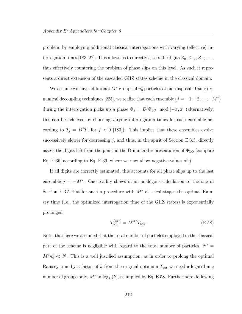
Appendix E: Appendices for Chapter 6
problem, by employing additional classical interrogations with varying (effective) in-
terrogation times [183, 27]. This allows us to directly assess the digits Z0, Z−1, Z−2 . . . ,
thus effectively countering the problem of phase slips on this level. As such it repre-
sents a direct extension of the cascaded GHZ states scheme in the classical domain.
We assume we have additional M∗ groups of n∗0 particles at our disposal. Using dy-
namical decoupling techniques [225], we realize that each ensemble (j = −1,−2 . . . ,−M∗)
during the interrogation picks up a phase Φj = DjΦLO mod [−π, π] (alternatively,
this can be achieved by choosing varying interrogation times for each ensemble ac-
cording to Tj = DjT , for j < 0 [183]). This implies that these ensembles evolve
successively slower for decreasing j, and thus, in the spirit of Section E.3.3, directly
assess the digits left from the point in the D-numeral representation of ΦLO [compare
Eq. E.36] according to Eq. E.39, where we now allow negative values of j.
If all digits are correctly estimated, this accounts for all phase slips up to the last
ensemble j = −M∗. One readily shows in an analogous calculation to the one in
Section E.3.5 that for such a procedure with M∗ classical stages the optimal Ram-
sey time (i.e., the optimized interrogation time of the GHZ states) is exponentially
prolonged
T(M∗)opt = DM∗Topt. (E.58)
Note, that here we assumed that the total number of particles employed in the classical
part of the scheme is negligible with regard to the total number of particles, N∗ =
M∗n∗0 N . This is a well justified assumption, as in order to prolong the optimal
Ramsey time by a factor of k from the original optimum Topt we need a logarithmic
number of groups only, M∗ ≈ logD(k), as implied by Eq. E.58. Furthermore, following
212
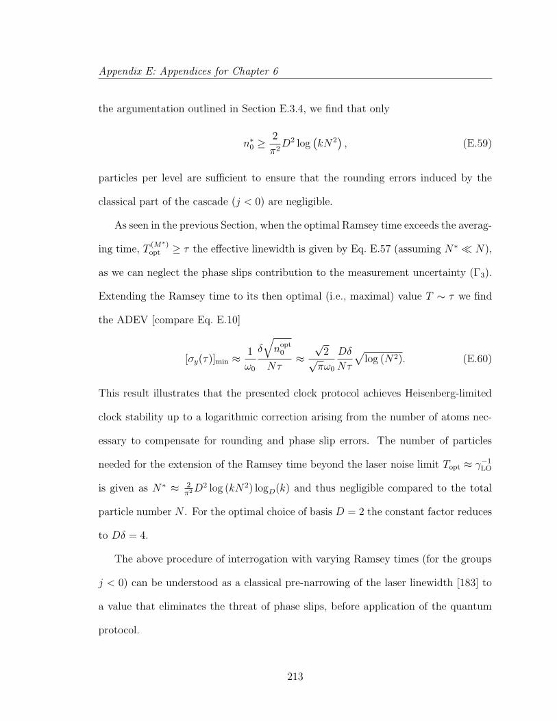
Appendix E: Appendices for Chapter 6
the argumentation outlined in Section E.3.4, we find that only
n∗0 ≥2
π2D2 log
(kN2
), (E.59)
particles per level are sufficient to ensure that the rounding errors induced by the
classical part of the cascade (j < 0) are negligible.
As seen in the previous Section, when the optimal Ramsey time exceeds the averag-
ing time, T(M∗)opt ≥ τ the effective linewidth is given by Eq. E.57 (assuming N∗ N),
as we can neglect the phase slips contribution to the measurement uncertainty (Γ3).
Extending the Ramsey time to its then optimal (i.e., maximal) value T ∼ τ we find
the ADEV [compare Eq. E.10]
[σy(τ)]min ≈1
ω0
δ√nopt
0
Nτ≈√
2√πω0
Dδ
Nτ
√log (N2). (E.60)
This result illustrates that the presented clock protocol achieves Heisenberg-limited
clock stability up to a logarithmic correction arising from the number of atoms nec-
essary to compensate for rounding and phase slip errors. The number of particles
needed for the extension of the Ramsey time beyond the laser noise limit Topt ≈ γ−1LO
is given as N∗ ≈ 2π2D
2 log (kN2) logD(k) and thus negligible compared to the total
particle number N . For the optimal choice of basis D = 2 the constant factor reduces
to Dδ = 4.
The above procedure of interrogation with varying Ramsey times (for the groups
j < 0) can be understood as a classical pre-narrowing of the laser linewidth [183] to
a value that eliminates the threat of phase slips, before application of the quantum
protocol.
213
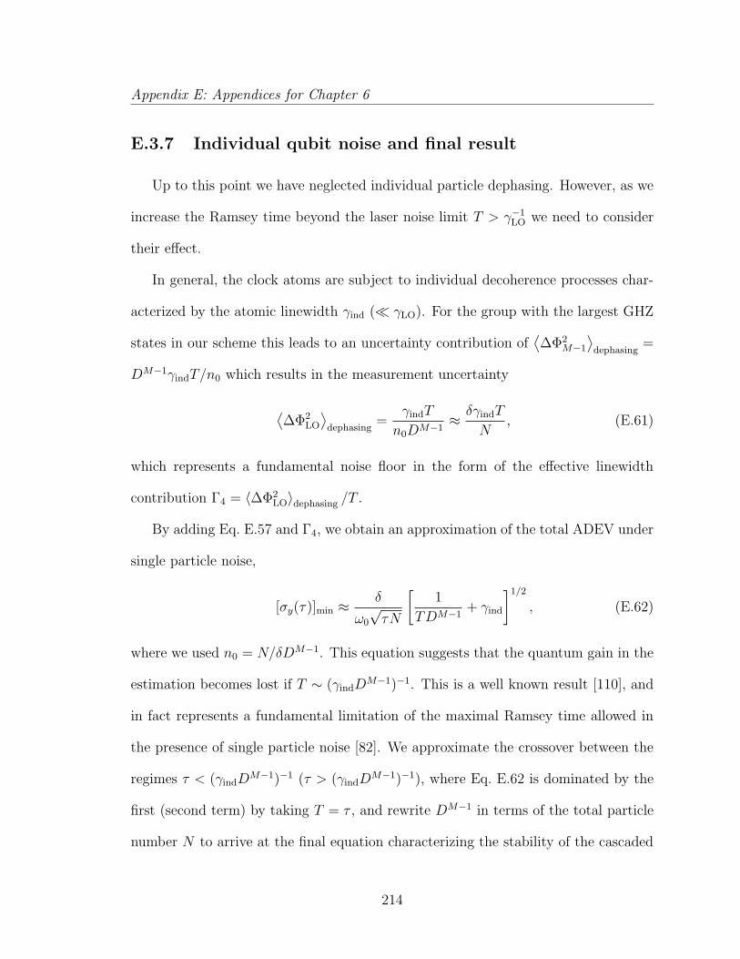
Appendix E: Appendices for Chapter 6
E.3.7 Individual qubit noise and final result
Up to this point we have neglected individual particle dephasing. However, as we
increase the Ramsey time beyond the laser noise limit T > γ−1LO we need to consider
their effect.
In general, the clock atoms are subject to individual decoherence processes char-
acterized by the atomic linewidth γind ( γLO). For the group with the largest GHZ
states in our scheme this leads to an uncertainty contribution of⟨∆Φ2
M−1
⟩dephasing
=
DM−1γindT/n0 which results in the measurement uncertainty
⟨∆Φ2
LO
⟩dephasing
=γindT
n0DM−1≈ δγindT
N, (E.61)
which represents a fundamental noise floor in the form of the effective linewidth
contribution Γ4 = 〈∆Φ2LO〉dephasing /T .
By adding Eq. E.57 and Γ4, we obtain an approximation of the total ADEV under
single particle noise,
[σy(τ)]min ≈δ
ω0
√τN
[1
TDM−1+ γind
]1/2
, (E.62)
where we used n0 = N/δDM−1. This equation suggests that the quantum gain in the
estimation becomes lost if T ∼ (γindDM−1)−1. This is a well known result [110], and
in fact represents a fundamental limitation of the maximal Ramsey time allowed in
the presence of single particle noise [82]. We approximate the crossover between the
regimes τ < (γindDM−1)−1 (τ > (γindD
M−1)−1), where Eq. E.62 is dominated by the
first (second term) by taking T = τ , and rewrite DM−1 in terms of the total particle
number N to arrive at the final equation characterizing the stability of the cascaded
214
Appendix E: Appendices for Chapter 6
GHZ scheme
[σy(τ)]min ≈1
ω0
√τN
[1
τN
2δ2D2
π2log(N2) + δγind
]1/2
. (E.63)
Again, for the choice of a binary basis D = 2 the constant factor is given as δD = 4.
In summary, we find that the cascaded GHZ scheme enables an optimal, Heisenberg-
limited laser stability for short averaging times τ up to a logarithmic correction. This
stability reaches the fundamental noise floor given by the single particle dephasing
for averaging times τ0 ≈ (γindDM−1)−1. Note, that in the limit N →∞ this crossover
value goes to zero, and the clock stability is given by the best possible stability al-
lowed by quantum mechanics for all τ . In comparison, classical protocols reach this
fundamental limit in the best case [183] at the fixed time τ ≈ γ−1ind. For averaging
times larger than this value τ ≥ γ−1ind the quantum protocol does not offer an ad-
vantage over an optimal classical protocol due to fundamental quantum metrological
bounds [82].
E.4 Analytic solution of xn = A exp[−1/x]
To carry out direct optimization of the Allan variance, we need to be able to solve
transcendental equations of the following form
xn = A exp
[−1
x
]. (E.64)
In this Section we obtain an analytic formula for the solution of this equation over
the domain x ∈ [0,∞), in the limiting case of A 1, where n is real. The sign of
n determines the number of solutions: In case of n > 0, there are three solutions:
215
Appendix E: Appendices for Chapter 6
xs,0 = 0, xs,1 1 and xs,2 1. In case of n ≤ 0, there is always a single solution,
xs,1 1. We are going to focus on the xs,1 =: xs solution, and give upper and lower
bounds, such that xl ≤ xs ≤ xu, and xu/xl → 1 as A→∞.
The general method of Taylor-expanding the right side of Eq. E.64 around x = 0
fails due to the non-analytic property of e−1/x function at zero, and forces us to choose
an alternate route. Here, we use a recursion formula, and prove its stability around
xs. Rearranging Eq. E.64 and turning it into a recursion f yields
xk =1
logA− n log xk−1
=: f(xk−1), (E.65)
The iteration of f is stable around the fixed point (f(xs) = xs), if and only if 1 >
|f ′(xs)| = xs|n|, which is true in the limit xs 1. Stability implies that the fix point
can be obtained as the limit
xs = limk→∞
xk = limk→∞
f [k](x0), (E.66)
if the x0 starting point is sufficiently close to xs, where f [k] denotes k iterations of f .
In case of n ≤ 0, f ′(xs) = nxs ≤ 0 therefore [f [k](x0)−f [k−1](x0)] is an alternating
sequence and we can quickly obtain upper (xu) and lower (xl) bounds by applying
the recursion f twice on x0 = 1:
xl = x1 =1
logA, xu = x2 =
1
logA+ n log logA, (E.67)
In case of n > 0 and x0 = 1, f [k](xs) is monotonically decreasing (since f ′(xs) > 0),
and we can safely choose the upper bound xu = x2. To obtain a lower bound, we
introduce a new variable ξ = − log x, and write Eq. E.65 as
ξk = log logA+ log
(1 +
n
logAξk−1
)(E.68)
≤ log logA+n
logAξk−1 =: g(ξk−1), (E.69)
216
Appendix E: Appendices for Chapter 6
where we used that log(1 + y) ≤ y, ∀y ∈ R+ and g is a new recursion. Since g
is a monotonically increasing function, the inequality holds for multiple iterations,
ξk ≤ g[k](ξ0), and eventually give the upper bound, − log xs = ξs ≤ limk→∞ g[k](ξ0).
In the limit of A 1, we can assume nlogA
< 1, and the sequence of iterations of
g becomes convergent. Due to its simple form, we can evaluate its limit in a closed
form, which results in the following upper bound for ξs and the corresponding lower
bound for xs.
ξs <log logA
1− nlogA
, → xs >
(1
logA
) 11− n
logA
. (E.70)
We can obtain an even better (and more conventional) lower bound by applying f
once more:
xl = f
[(1
logA
) 11− n
logA
]=
1
logA+ 11− n
logAn log logA
(E.71)
For both signs of n, xl logA → 1, xu logA → 1, and xu/xl → 1 as A → ∞, from
which we conclude that
limA→∞
(xs logA) = 1. (E.72)
For large enough A, we can approximate xs with [logA]−1, and the relative error is
bounded by |n| log logAlogA
.
E.5 Upper bound on the tail of the distribution of
the estimated phase
The probability of rounding errors is given an upper bound in order to obtain a
more tractable form for optimization.
217
Appendix E: Appendices for Chapter 6
E.5.1 Upper bound on the tail of the binomial distribution
Here we derive an upper bound for the binomial distribution
P(k) =
(n
k
)pk(1− p)n−k. (E.73)
Central limit theorem implies that for large enough n, P(k) can be approximated
with the normal distribution, N (np, np(1− p)), however, one can be concerned with
the fact that this underestimates the tail of P(k). Here we give F (k) as a strict upper
bound on P(k),
P(k) < F (k) = exp
[−2(n− 1)
(k
n− p)2]. (E.74)
To see that F (k) is indeed an upper bound of P(k) for all n, p and k, let us
examine the logarithm of the binomial distribution P(k = ny),
L(y) = log
(n
ny
)+ ny log p+ n(1− y) log(1− p), (E.75)
where 0 ≤ y ≤ 1. The properties, we are interested in, are
• L(y) < 0 for all y, since P(k) < 1,
• ∂∂yL(y)
∣∣∣y=p
= 0, and positive for y < p and negative for y > p, since L(y) = max
at y = p.
• ∂2
∂y2L(y) = ∂2
∂y2
(nny
)= −n2
(ψ1[1 + n(1 − y)] + ψ1[1 + ny]
), where ψ1(x) =
ddx
log Γ(x), the first polygamma function.
By analyzing the series expansion of ψ1(1 + η) for large and small η arguments,
ψ1(1 + η) =1
η− 1
2η2+O(η−3) η 1 (E.76)
ψ1(1 + η) =π2
6− 2.404η +
π4
30η2 +O(η3) η 1, (E.77)
218
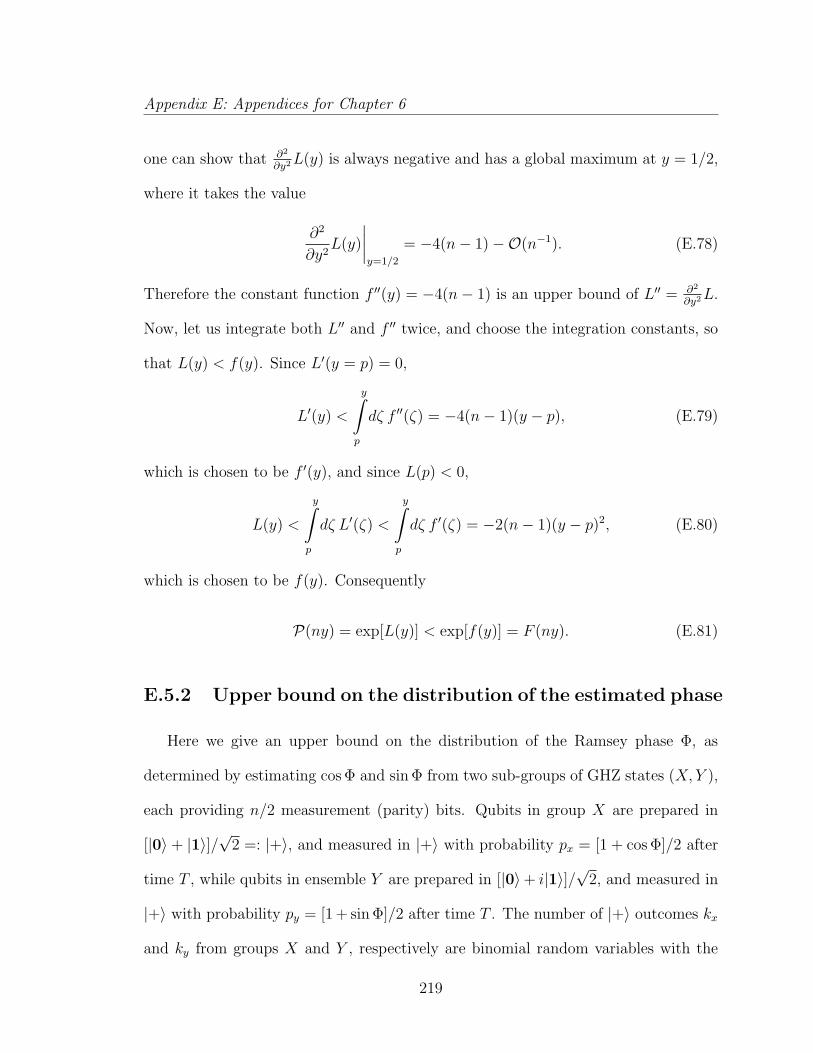
Appendix E: Appendices for Chapter 6
one can show that ∂2
∂y2L(y) is always negative and has a global maximum at y = 1/2,
where it takes the value
∂2
∂y2L(y)
∣∣∣∣y=1/2
= −4(n− 1)−O(n−1). (E.78)
Therefore the constant function f ′′(y) = −4(n− 1) is an upper bound of L′′ = ∂2
∂y2L.
Now, let us integrate both L′′ and f ′′ twice, and choose the integration constants, so
that L(y) < f(y). Since L′(y = p) = 0,
L′(y) <
y∫
p
dζ f ′′(ζ) = −4(n− 1)(y − p), (E.79)
which is chosen to be f ′(y), and since L(p) < 0,
L(y) <
y∫
p
dζ L′(ζ) <
y∫
p
dζ f ′(ζ) = −2(n− 1)(y − p)2, (E.80)
which is chosen to be f(y). Consequently
P(ny) = exp[L(y)] < exp[f(y)] = F (ny). (E.81)
E.5.2 Upper bound on the distribution of the estimated phase
Here we give an upper bound on the distribution of the Ramsey phase Φ, as
determined by estimating cos Φ and sin Φ from two sub-groups of GHZ states (X, Y ),
each providing n/2 measurement (parity) bits. Qubits in group X are prepared in
[|0〉 + |1〉]/√
2 =: |+〉, and measured in |+〉 with probability px = [1 + cos Φ]/2 after
time T , while qubits in ensemble Y are prepared in [|0〉+ i|1〉]/√
2, and measured in
|+〉 with probability py = [1 + sin Φ]/2 after time T . The number of |+〉 outcomes kx
and ky from groups X and Y , respectively are binomial random variables with the
219
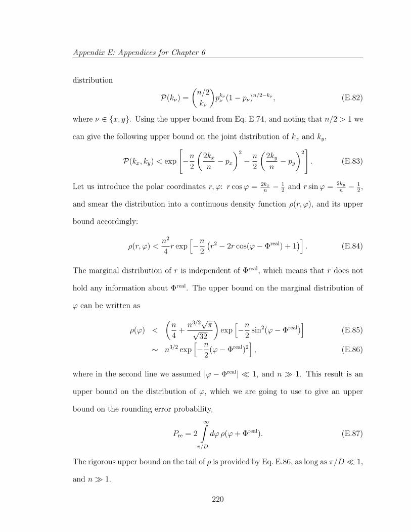
Appendix E: Appendices for Chapter 6
distribution
P(kν) =
(n/2
kν
)pkνν (1− pν)n/2−kν , (E.82)
where ν ∈ x, y. Using the upper bound from Eq. E.74, and noting that n/2 > 1 we
can give the following upper bound on the joint distribution of kx and ky,
P(kx, ky) < exp
[−n
2
(2kxn− px
)2
− n
2
(2kyn− py
)2]. (E.83)
Let us introduce the polar coordinates r, ϕ: r cosϕ = 2kxn− 1
2and r sinϕ = 2ky
n− 1
2,
and smear the distribution into a continuous density function ρ(r, ϕ), and its upper
bound accordingly:
ρ(r, ϕ) <n2
4r exp
[−n
2
(r2 − 2r cos(ϕ− Φreal) + 1
)]. (E.84)
The marginal distribution of r is independent of Φreal, which means that r does not
hold any information about Φreal. The upper bound on the marginal distribution of
ϕ can be written as
ρ(ϕ) <
(n
4+n3/2√π√
32
)exp
[−n
2sin2(ϕ− Φreal)
](E.85)
∼ n3/2 exp[−n
2(ϕ− Φreal)2
], (E.86)
where in the second line we assumed |ϕ − Φreal| 1, and n 1. This result is an
upper bound on the distribution of ϕ, which we are going to use to give an upper
bound on the rounding error probability,
Pre = 2
∞∫
π/D
dϕ ρ(ϕ+ Φreal). (E.87)
The rigorous upper bound on the tail of ρ is provided by Eq. E.86, as long as π/D 1,
and n 1.
220

Appendix E: Appendices for Chapter 6
E.6 Threshold fidelity
In this section we estimate the fidelity of the pairwise entangling operations re-
quired to keep the benefit of quantum enhancement. (Following closely the analysis in
the supplementary of [121]) In the GHZ state generation step of every cycle, n copies
of the cascade are initialized. This requires N/n pairwise entangling operations per
copy. Among other unitary operations, this is likely to be the bottleneck. If one
entangling operation can be performed with fidelity F = exp[−ε] (ε 1), then N/n
repetitions succeed with fidelity Ftotal = FN/n = exp[−Nε/n].
Whenever a copy fails on level i of the cascade, its measurement result φi becomes
completely random. This happens with probability (1−Ftotal). In the meantime, with
probability Ftotal, the result is consistent with φi = φreal, where φreal is the actual value
of φi. Out of the n copies nFtotal contributes to a peak centered at φreal, with width
of 1/√Ftotaln and weight Ftotal, while the rest contributes to a uniform distribution
with weight (1− Ftotal): The expectation value of φi is still
〈φi〉 = φreal, (E.88)
but the variance is
Var(φi) ≈1
n+π2
3(1− Ftotal). (E.89)
The threshold fidelity Fth is defined by the criteria that if F ≥ Fth, then Var(φi) ≈
1/n. If this is satisfied, then losing the information from some of the copies does not
deteriorate the precision significantly.
This requires 1−Ftotal <3π2n
, while Ftotal = exp[−εN/n] from above. From these,
221
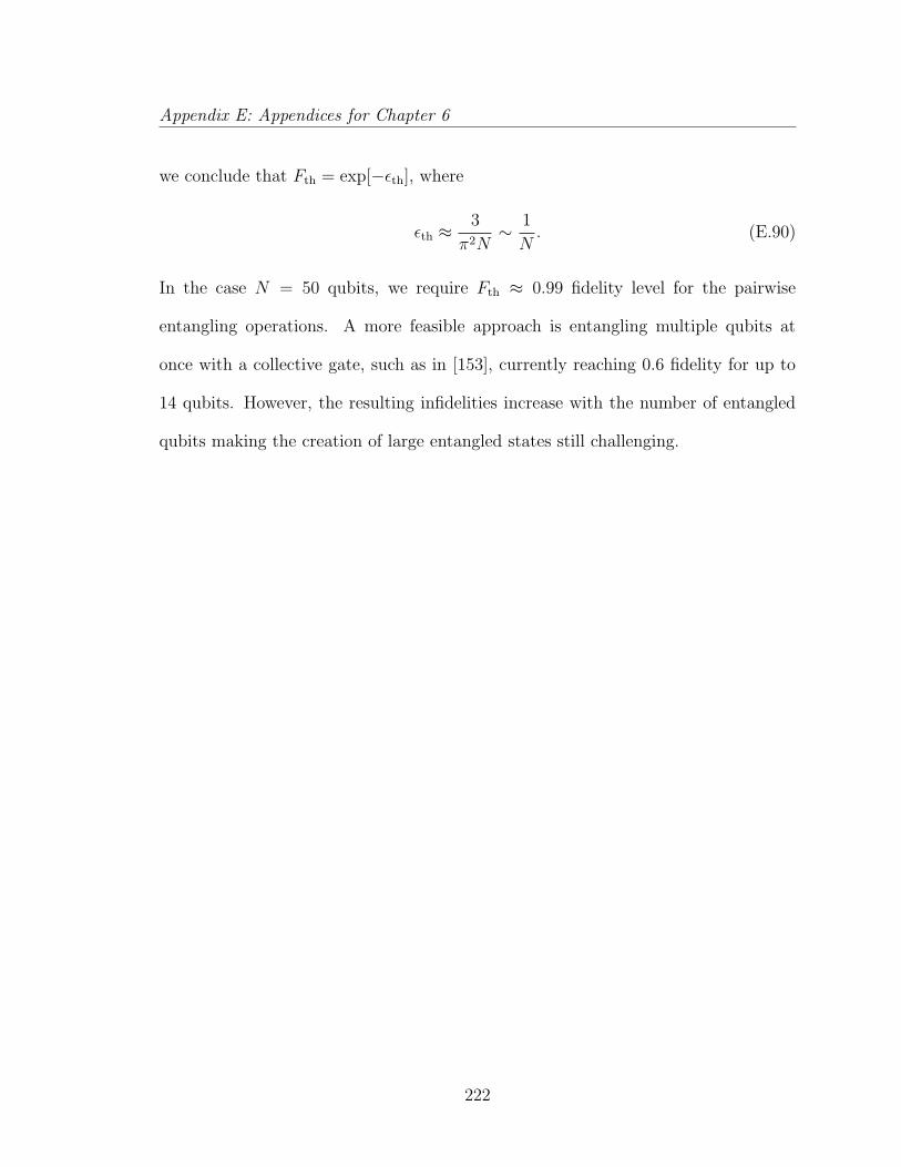
Appendix E: Appendices for Chapter 6
we conclude that Fth = exp[−εth], where
εth ≈3
π2N∼ 1
N. (E.90)
In the case N = 50 qubits, we require Fth ≈ 0.99 fidelity level for the pairwise
entangling operations. A more feasible approach is entangling multiple qubits at
once with a collective gate, such as in [153], currently reaching 0.6 fidelity for up to
14 qubits. However, the resulting infidelities increase with the number of entangled
qubits making the creation of large entangled states still challenging.
222
Appendix F
Appendices for Chapter 7
F.1 GHZ cascade in a network of K clocks
Here, we discuss the details of using quantum correlated states constructed out of
N ′ = Kn qubits, equally distributed among K clocks, namely the GHZ state of the
form
[|00 . . . 0〉+ eiχ|11 . . . 1〉]/√
2, (F.1)
where |qq . . . q〉 = |q〉⊗N ′ , q ∈ 0, 1. Entanglement has two effects here: First, it
makes the phase of such a GHZ state, χ, sensitive to the accumulated phase of the
center-of-mass of all the K independent local oscillators, (each located at one of the
clocks) ΦCOM =∑K
j=1 Φ(j)/K, where Φ(j) =∫ T
0dt (ω(j)(t) − ω0) is the accumulated
phase of the LO at clock j, during the interrogation time T , here ω(j)(t) is the
instantaneous frequency of the LO, while ω0 is the transition frequency of the clock
223
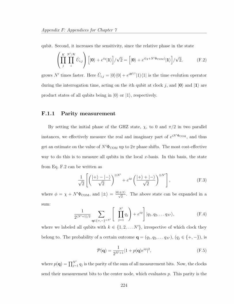
Appendix F: Appendices for Chapter 7
qubit. Second, it increases the sensitivity, since the relative phase in the state
K∏
j
N ′/K∏
i
Ui,j
[|0〉+ eiχ|1〉
]/√
2 =[|0〉+ ei(χ+N ′ΦCOM)|1〉
]/√
2, (F.2)
grows N ′ times faster. Here Ui,j = |0〉〈0| + eiΦ(j) |1〉〈1| is the time evolution operator
during the interrogation time, acting on the ith qubit at clock j, and |0〉 and |1〉 are
product states of all qubits being in |0〉 or |1〉, respectively.
F.1.1 Parity measurement
By setting the initial phase of the GHZ state, χ, to 0 and π/2 in two parallel
instances, we effectively measure the real and imaginary part of eiN′ΦCOM , and thus
get an estimate on the value of N ′ΦCOM up to 2π phase shifts. The most cost-effective
way to do this is to measure all qubits in the local x-basis. In this basis, the state
from Eq. F.2 can be written as
1√2
[( |+〉 − |−〉√2
)⊗N ′+ eiφ
( |+〉+ |−〉√2
)⊗N ′], (F.3)
where φ = χ + N ′ΦCOM, and |±〉 = |0〉±|1〉√2
. The above state can be expanded in a
sum:
1
2(N ′+1)/2
∑
q∈+,−×N′
[(N ′∏
j=1
qj
)+ eiφ
]|q1, q2, . . . qN ′〉, (F.4)
where we labeled all qubits with k ∈ 1, 2, . . . N ′, irrespective of which clock they
belong to. The probability of a certain outcome q = (q1, q2, . . . qN ′), (qj ∈ +,−), is
P(q) =1
2N ′+1|1 + p(q)eiφ|2, (F.5)
where p(q) =∏N ′
j=1 qj is the parity of the sum of all measurement bits. Now, the clocks
send their measurement bits to the center node, which evaluates p. This parity is the
224
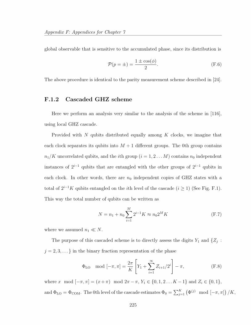
Appendix F: Appendices for Chapter 7
global observable that is sensitive to the accumulated phase, since its distribution is
P(p = ±) =1± cos(φ)
2. (F.6)
The above procedure is identical to the parity measurement scheme described in [24].
F.1.2 Cascaded GHZ scheme
Here we perform an analysis very similar to the analysis of the scheme in [116],
using local GHZ cascade.
Provided with N qubits distributed equally among K clocks, we imagine that
each clock separates its qubits into M + 1 different groups. The 0th group contains
n1/K uncorrelated qubits, and the ith group (i = 1, 2 . . .M) contains n0 independent
instances of 2i−1 qubits that are entangled with the other groups of 2i−1 qubits in
each clock. In other words, there are n0 independent copies of GHZ states with a
total of 2i−1K qubits entangled on the ith level of the cascade (i ≥ 1) (See Fig. F.1).
This way the total number of qubits can be written as
N = n1 + n0
M∑
i=1
2i−1K ≈ n02MK (F.7)
where we assumed n1 N .
The purpose of this cascaded scheme is to directly assess the digits Y1 and Zj :
j = 2, 3, . . . in the binary fraction representation of the phase
ΦLO mod [−π, π] =2π
K
[Y1 +
∞∑
i=1
Zi+1/2i
]− π, (F.8)
where x mod [−π, π] = (x+π) mod 2π−π, Y1 ∈ 0, 1, 2 . . . K− 1 and Zi ∈ 0, 1,
and ΦLO = ΦCOM. The 0th level of the cascade estimates Φ0 =∑K
j=1
(Φ(j) mod [−π, π]
)/K,
225
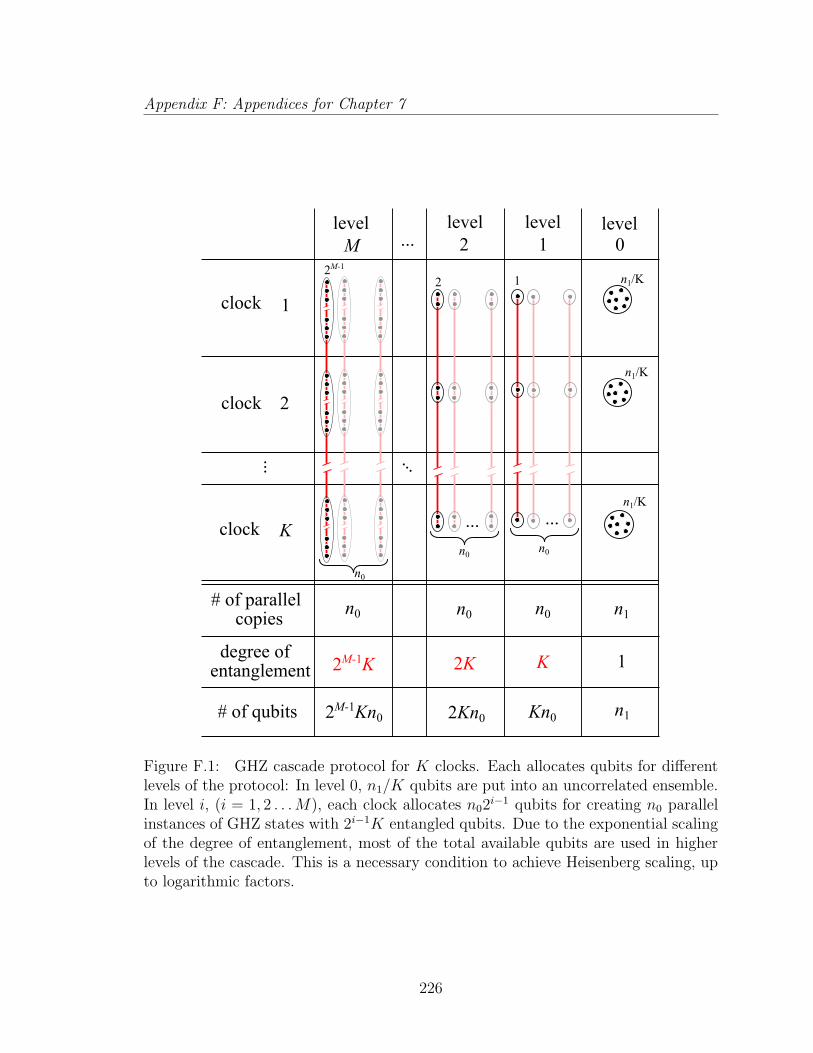
Appendix F: Appendices for Chapter 7
Figure F.1: GHZ cascade protocol for K clocks. Each allocates qubits for differentlevels of the protocol: In level 0, n1/K qubits are put into an uncorrelated ensemble.In level i, (i = 1, 2 . . .M), each clock allocates n02i−1 qubits for creating n0 parallelinstances of GHZ states with 2i−1K entangled qubits. Due to the exponential scalingof the degree of entanglement, most of the total available qubits are used in higherlevels of the cascade. This is a necessary condition to achieve Heisenberg scaling, upto logarithmic factors.
226
Appendix F: Appendices for Chapter 7
and every ith level after that estimates Φi = K2i−1ΦLO mod [−π, π]. In other words,
every level of the cascade is sensitive to a different multiple of the LO phase ΦLO
(mod 2π). After the separate measurements of the levels, each provide an estimate
to Φi which can be combined to obtain the best estimate for ΦLO. Here we describe
this using the digits Y1 and Zi as intermediate quantities, which are calculated from
Φi the following way,
Y1 = [K(Φ0 + π)− (Φ1 + π)] /(2π), (F.9)
Zi = [2(Φi−1 + π)− (Φi + π)] /(2π), (F.10)
for i = 2, 3, . . .M .
The last group (i = M) contains GHZ states with the most entangled qubits.
These are the ones with the fastest evolving phase, and therefore they provide the
best resolution on ΦLO. Since there are n0 independent instances, their phase ΦM =
2π∑∞
i=1 ZM+i/2i is known up to the uncertainty, 〈∆Φ2
M〉pr = 1n0
,
Assuming that all lower digits Y1, Zj|j = 2 . . .M have been determined cor-
rectly, this results in the total measurement uncertainty for ΦLO:
⟨∆Φ2
LO
⟩pr
=〈∆Φ2
M〉pr
(2M−1K)2=
4n0
N2, (F.11)
where, for the moment, we neglected individual qubit noise and assumed ΦLO ∈
[−π, π]. However, in general, the estimation of the lower digits will not be perfect.
In the following section we investigate the effect of these rounding errors on the final
measurement accuracy. From this analysis we find the optimal number of copies n0
and n1.
227
Appendix F: Appendices for Chapter 7
F.1.3 Rounding errors
Whenever |Φest0 −Φ0| > π/K, or |Φest
i −Φi| > π/2 (for i ≥ 1), we make a mistake
by under- or overestimating the number of phase slips Y1 or Zi+1, respectively. To
minimize the effect of this error, we need to optimize how the total of N qubits are
distributed among the various levels of the cascade. In other words we need to find
n0,opt and n1,opt.
The probability that a rounding error occurs during the estimation of Zi+1 is
Pi,re = 2
∞∫
π/2
dφ ρi(φ+ Φi) ≤ 2
∞∫
π/2
dφ1
s3i
exp
[− φ2
2s2i
](F.12)
where φ = Φesti −Φi, and ρi is the conditional density function of Φest
i for a given real
Φi, and s2i = Var(Φest
i −Φi) = 1/n0 for i ≥ 1, and s20 = 〈∆Φ2
0〉pr = 1K2
∑Kj=1
⟨(∆Φ(j))2
⟩pr
=
1/n1, since⟨(∆Φ(j))2
⟩pr
= Kn1
for all j. The upper bound for ρi is obtained by us-
ing the following upper bound for any binomial distribution:(nk
)pk(1 − p)n−k ≤
exp[−n(kn− p)2]. (For details, see Appendix E.) The resulting probabilities, after
dropping the higher order terms in the asymptotic expansions, are
P0,re ≈2K
πn
1/21 exp
[−n1π
2
2K2
], (F.13)
Pi,re ≈4
πn
1/20 exp
[−n0π
2
8
](i ≥ 1). (F.14)
These approximate formulas are valid for n0 ≥ 5, as we have checked numerically.
The phase shift imposed on the estimate of ΦLO by a manifested rounding error
of Y1 is 2π/K and of Zi is 2π/(K2i−1), for i = 2, 3 . . .M . This results in the total
variance contribution,
⟨∆Φ2
LO
⟩re
=
(2π
K
)2[P0,re +
M∑
i=2
Pi−1,re(2−i+1)2
]≈(
2π
K
)2 [P0,re +
1
3Pi−1,re
].
(F.15)
228
Appendix F: Appendices for Chapter 7
We simplify this expression by choosing n1 so that P0,re ≈ 23Pi,re:
n1 = αK2n0, (F.16)
where α ≈ max
1 , 2
π2n0log
(3K2
√8
πn1/20
) n0, K. With this choice, we can write
the rounding error contribution as
⟨∆Φ2
LO
⟩re≈ 16π
K2n
1/20 exp
[−n0π
2
8
]. (F.17)
We note that the amount of extra resources needed for the 0th level is marginally
small, since the total qubit number can be expressed as
N = n1 + n0KM∑
i=1
2i−1 = n0K(αK + 2M − 2) ≈ n0K2M , (F.18)
under the assumption K 2M .
By adding the two error contributions from Eq. F.11 and Eq. F.17, we obtain the
corresponding Allan-variance in the stationary noise approximation,
σ2y(τ) =
1
ω20τT
⟨∆Φ2
LO
⟩=:
1
ω20τ
[Γ1 + Γ2] = (F.19)
=1
ω20τ
[4n0
N2T+
16π
K2Tn
1/20 exp
[−n0π
2
8
]](F.20)
Now, let us find the optimal value of n0. We write Γ1 + Γ2, using the new variable
x = 8π2
1n0
, as
Γ1 + Γ2 =4
T
(8
π2
1
xN2+
√32
K2
1
x1/2exp
[−1
x
]). (F.21)
Taking the derivative with respect to x and equating it with 0, while using the as-
sumption x 1 results in Γ2 ≈ xoptΓ1 Γ1, which can be written as the following
transcendental equation for the optimal value, xopt,
x1/2opt ≈
π2N2
√8K2
exp
[− 1
xopt
]. (F.22)
229
Appendix F: Appendices for Chapter 7
The general solution of any equation of the form xν = A exp[−1/x], in the limit of
A 1 and x 1, is x = [log(A)]−1 . (For details, see Appendix E.) Using this result
we can write
xopt ≈[log
(π2
√8
N2
K2
)]−1
∼ [2 log(N/K)]−1 (F.23)
n0,opt ≈8
π2
1
xopt
∼(
4
π
)2
log (N/K) . (F.24)
For the realistic case of N/K 1, indeed xopt 1, and the corresponding minimal
value of Γ1 + Γ2 is
[Γ1 + Γ2]min ≈ Γ1(xopt) =
(8
π
)2log(N/K)
N2T. (F.25)
This result indicates that, in terms of qubit number, only a logarithmic extra cost is
required to achieve the Heisenberg limit.
F.1.4 Phase slip errors
Although the cascade is designed to detect phase slips of all levels i = 1, 2 . . .M ,
a possible phase wrap of level i = 0 remains undetected. Since the qubits at different
clocks are interrogated independently on the 0th level, each of them estimates the
phase of the corresponding LO, Φ(j)0 (j = 1, 2, . . . K), and not ΦLO, the phase accu-
mulated by the local oscillator. The probability of Φ(j)0 falling outside the interval
[−π, π] at least once during the total measurement time τ is
Pj,slip = 2τ
T
∞∫
π
dφ1√
2πγLOTexp
[− φ2
2γLOT
]≈
≈ τ
T
√2
π3/2
√γLOT exp
[− π2
2γLOT
], (F.26)
230
Appendix F: Appendices for Chapter 7
where γLO is the linewidth of the local oscillator at clock j, corresponding to a white
noise spectrum, resulting in a constant phase diffusion over the interrogation time T ,
(which is assumed to be approximately equal to the cycle time). The approximate
form above is obtained by neglecting the higher order terms in the asymptotic series
expansion under the assumption γLOT 1. (The white noise assumption can be
relaxed to include more realistic LO noise spectra. However, numerical simulations
have shown that, for a LO subject to a feedback loop, the low frequency noise is
essentially white even though the LO may have more complicated noise spectrum,
such as 1/f noise. Therefore the results derived for white noise applies up to a constant
prefactor. [27] We proceed with the white noise assumption for simplicity.) Once such
a phase slip happens, it introduces a 2π phase shift in Φ(j)0 , and therefore contributes
to its overall uncertainty with⟨
(∆Φ(j)0 )2
⟩= (2π)2Pj,slip. Physically Φ0 is the phase
of the COM signal, that the center can obtain after averaging the frequencies of
all K local oscillators with equal weights, Φ0 = ΦCOM =∑K
j=1 Φ(j)0 /K, therefore
〈∆Φ20〉 = 1
K2
∑Kj=1
⟨(∆Φ
(j)0 )2
⟩= 1
K
⟨(∆Φ
(j)0 )2
⟩, where we assumed that the LOs are
independent but they have the same linewidth, γLO. Therefore the noise of the COM
phase is reduced compared to the individual LOs. Since Φ0 = ΦLO, the above results
in the following variance contribution
⟨∆Φ2
LO
⟩slip
=√
32πτγ
1/2LO
T 1/2Kexp
[− π2
2γLOT
]. (F.27)
After adding this error to the previously minimized projection and rounding er-
ror terms (from Eq. F.25), we obtain the corresponding Allan-variance, σ2y(τ) =
231
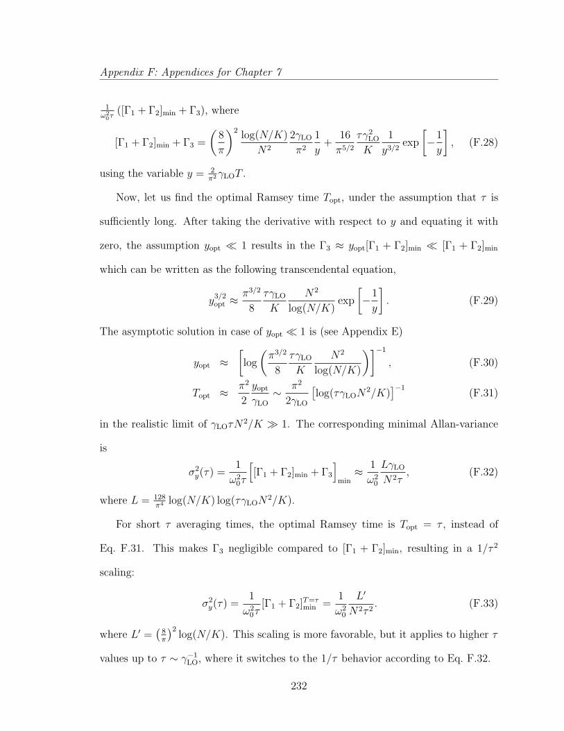
Appendix F: Appendices for Chapter 7
1ω2
0τ([Γ1 + Γ2]min + Γ3), where
[Γ1 + Γ2]min + Γ3 =
(8
π
)2log(N/K)
N2
2γLO
π2
1
y+
16
π5/2
τγ2LO
K
1
y3/2exp
[−1
y
], (F.28)
using the variable y = 2π2γLOT .
Now, let us find the optimal Ramsey time Topt, under the assumption that τ is
sufficiently long. After taking the derivative with respect to y and equating it with
zero, the assumption yopt 1 results in the Γ3 ≈ yopt[Γ1 + Γ2]min [Γ1 + Γ2]min
which can be written as the following transcendental equation,
y3/2opt ≈
π3/2
8
τγLO
K
N2
log(N/K)exp
[−1
y
]. (F.29)
The asymptotic solution in case of yopt 1 is (see Appendix E)
yopt ≈[log
(π3/2
8
τγLO
K
N2
log(N/K)
)]−1
, (F.30)
Topt ≈π2
2
yopt
γLO
∼ π2
2γLO
[log(τγLON
2/K)]−1
(F.31)
in the realistic limit of γLOτN2/K 1. The corresponding minimal Allan-variance
is
σ2y(τ) =
1
ω20τ
[[Γ1 + Γ2]min + Γ3
]min≈ 1
ω20
LγLO
N2τ, (F.32)
where L = 128π4 log(N/K) log(τγLON
2/K).
For short τ averaging times, the optimal Ramsey time is Topt = τ , instead of
Eq. F.31. This makes Γ3 negligible compared to [Γ1 + Γ2]min, resulting in a 1/τ 2
scaling:
σ2y(τ) =
1
ω20τ
[Γ1 + Γ2]T=τmin =
1
ω20
L′
N2τ 2. (F.33)
where L′ =(
8π
)2log(N/K). This scaling is more favorable, but it applies to higher τ
values up to τ ∼ γ−1LO, where it switches to the 1/τ behavior according to Eq. F.32.
232
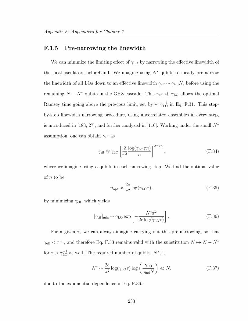
Appendix F: Appendices for Chapter 7
F.1.5 Pre-narrowing the linewidth
We can minimize the limiting effect of γLO by narrowing the effective linewidth of
the local oscillators beforehand. We imagine using N∗ qubits to locally pre-narrow
the linewidth of all LOs down to an effective linewidth γeff ∼ γindN , before using the
remaining N − N∗ qubits in the GHZ cascade. This γeff γLO allows the optimal
Ramsey time going above the previous limit, set by ∼ γ−1LO in Eq. F.31. This step-
by-step linewidth narrowing procedure, using uncorrelated ensembles in every step,
is introduced in [183, 27], and further analyzed in [116]. Working under the small N∗
assumption, one can obtain γeff as
γeff ≈ γLO
[2
π2
log(γLOτn)
n
]N∗/n, (F.34)
where we imagine using n qubits in each narrowing step. We find the optimal value
of n to be
nopt ≈2e
π2log(γLOτ), (F.35)
by minimizing γeff , which yields
[γeff ]min ∼ γLO exp
[− N∗π2
2e log(γLOτ)
]. (F.36)
For a given τ , we can always imagine carrying out this pre-narrowing, so that
γeff < τ−1, and therefore Eq. F.33 remains valid with the substitution N 7→ N −N∗
for τ > γ−1LO as well. The required number of qubits, N∗, is
N∗ ∼ 2e
π2log(γLOτ) log
(γLO
γindN
) N. (F.37)
due to the exponential dependence in Eq. F.36.
233
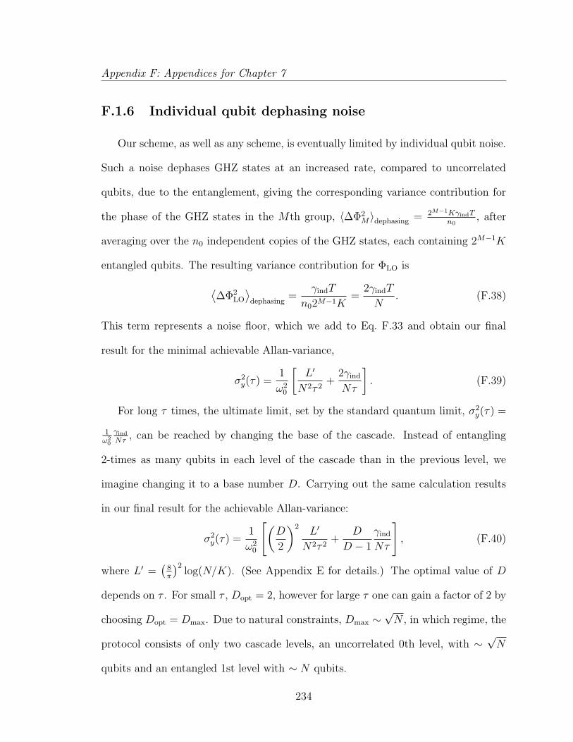
Appendix F: Appendices for Chapter 7
F.1.6 Individual qubit dephasing noise
Our scheme, as well as any scheme, is eventually limited by individual qubit noise.
Such a noise dephases GHZ states at an increased rate, compared to uncorrelated
qubits, due to the entanglement, giving the corresponding variance contribution for
the phase of the GHZ states in the Mth group, 〈∆Φ2M〉dephasing = 2M−1KγindT
n0, after
averaging over the n0 independent copies of the GHZ states, each containing 2M−1K
entangled qubits. The resulting variance contribution for ΦLO is
⟨∆Φ2
LO
⟩dephasing
=γindT
n02M−1K=
2γindT
N. (F.38)
This term represents a noise floor, which we add to Eq. F.33 and obtain our final
result for the minimal achievable Allan-variance,
σ2y(τ) =
1
ω20
[L′
N2τ 2+
2γind
Nτ
]. (F.39)
For long τ times, the ultimate limit, set by the standard quantum limit, σ2y(τ) =
1ω2
0
γind
Nτ, can be reached by changing the base of the cascade. Instead of entangling
2-times as many qubits in each level of the cascade than in the previous level, we
imagine changing it to a base number D. Carrying out the same calculation results
in our final result for the achievable Allan-variance:
σ2y(τ) =
1
ω20
[(D
2
)2L′
N2τ 2+
D
D − 1
γind
Nτ
], (F.40)
where L′ =(
8π
)2log(N/K). (See Appendix E for details.) The optimal value of D
depends on τ . For small τ , Dopt = 2, however for large τ one can gain a factor of 2 by
choosing Dopt = Dmax. Due to natural constraints, Dmax ∼√N , in which regime, the
protocol consists of only two cascade levels, an uncorrelated 0th level, with ∼√N
qubits and an entangled 1st level with ∼ N qubits.
234
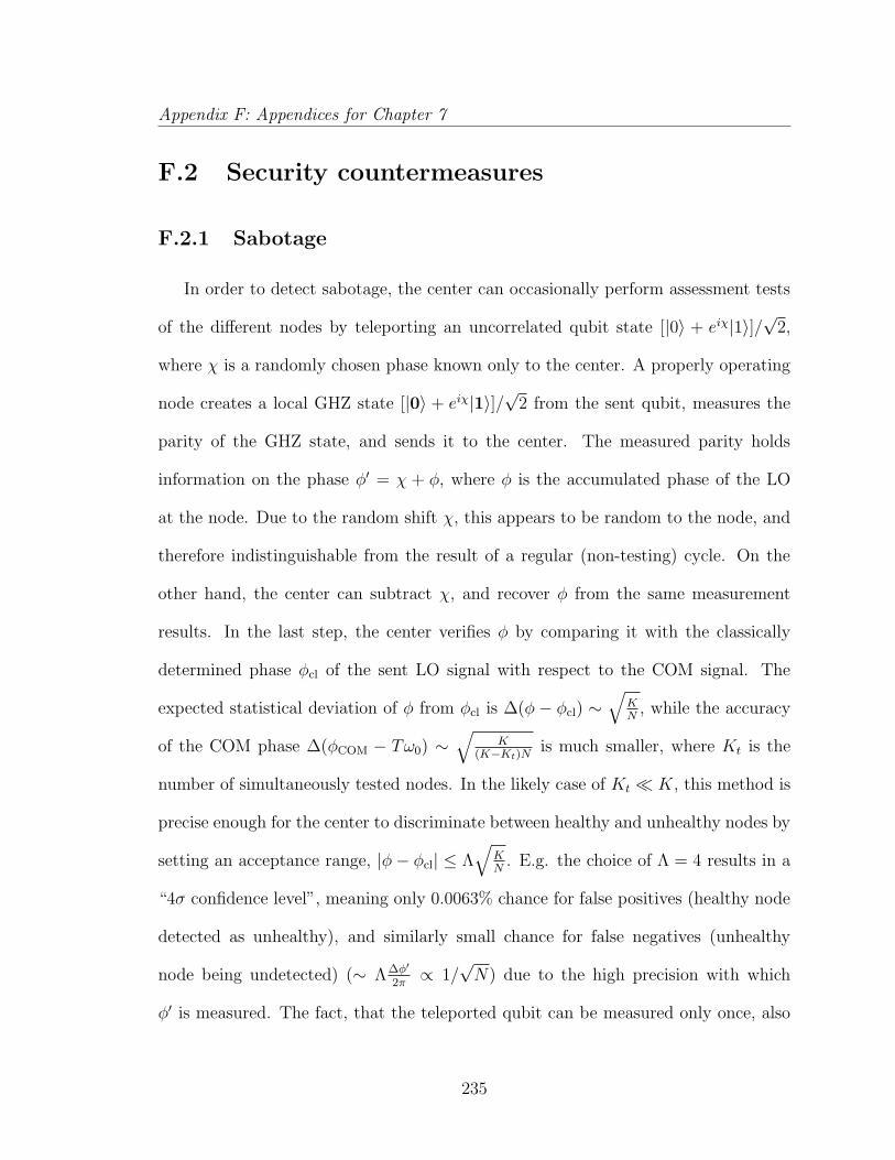
Appendix F: Appendices for Chapter 7
F.2 Security countermeasures
F.2.1 Sabotage
In order to detect sabotage, the center can occasionally perform assessment tests
of the different nodes by teleporting an uncorrelated qubit state [|0〉 + eiχ|1〉]/√
2,
where χ is a randomly chosen phase known only to the center. A properly operating
node creates a local GHZ state [|0〉 + eiχ|1〉]/√
2 from the sent qubit, measures the
parity of the GHZ state, and sends it to the center. The measured parity holds
information on the phase φ′ = χ + φ, where φ is the accumulated phase of the LO
at the node. Due to the random shift χ, this appears to be random to the node, and
therefore indistinguishable from the result of a regular (non-testing) cycle. On the
other hand, the center can subtract χ, and recover φ from the same measurement
results. In the last step, the center verifies φ by comparing it with the classically
determined phase φcl of the sent LO signal with respect to the COM signal. The
expected statistical deviation of φ from φcl is ∆(φ − φcl) ∼√
KN
, while the accuracy
of the COM phase ∆(φCOM − Tω0) ∼√
K(K−Kt)N is much smaller, where Kt is the
number of simultaneously tested nodes. In the likely case of Kt K, this method is
precise enough for the center to discriminate between healthy and unhealthy nodes by
setting an acceptance range, |φ− φcl| ≤ Λ√
KN
. E.g. the choice of Λ = 4 results in a
“4σ confidence level”, meaning only 0.0063% chance for false positives (healthy node
detected as unhealthy), and similarly small chance for false negatives (unhealthy
node being undetected) (∼ Λ∆φ′
2π∝ 1/
√N) due to the high precision with which
φ′ is measured. The fact, that the teleported qubit can be measured only once, also
235
Appendix F: Appendices for Chapter 7
prevents the nodes from discovering that it is being tested. In fact the center performs
a very simple blind quantum computing task using the resources of the other clocks,
see [50, 34, 140].
F.2.2 Eavesdropping
Provided that the threat of sabotage is effectively eliminated, we turn our attention
to the problem of eavesdropping. Eavesdroppers would try to intercept the sent LO
signals, and synthesize the stabilized νCOM for themselves. Our protocol minimizes
the attainable information of this strategy by prescribing that only the non-stabilized
LO signals are sent through classical channels. This requires the feedback to be
applied to the LO signal after some of it has been split off by a beam splitter, and
the center to integrate the generated feedback in time. Alternatively, eavesdroppers
could try intercepting the LO signals and the feedback signals, and gain access to
the same information, the center has. This can be prevented by encoding the radio
frequency feedback signal with phase modulation according to a shared secret key.
Since such a key can be shared securely with quantum key distribution, this protocol
keeps the feedback signal hidden from outsiders. As a result, even the hardest-working
eavesdropper, who intercepts all LO signals, is able to access only the non-stabilized
COM signal, and the stabilized COM signal remains accessible exclusively to parties
involved in the collaboration.
236
Appendix F: Appendices for Chapter 7
F.2.3 Rotating center role
Since the center works as a hub for all information, ensuring its security has the
highest priority. In a scenario, where a small number of nodes (without knowing
which) cannot be trusted enough to play the permanent role of the center, a rotating
stage scheme can be used. By passing the role of the center around, the potential
vulnerability of the network due to one untrustworthy site is substantially lowered.
This requires a fully connected network and a global scheme for assigning the role of
the center.
F.3 Network operation
F.3.1 Different degree of feedback
Apart from the full feedback, described in the main text, alternatively, the center
can be operated to provide restricted feedback information to the nodes. If the center
sends the averaged error signal δCOM only, the LOs at the nodes will not benefit from
the enhanced stability and only the center can access the stabilized signal. Of course
the LO at each node will have its own local feedback to keep it within a reasonable
frequency range around the clock transition. Such a ’safe’ operational mode allows
the center node to use the resources of other nodes, while keeping the world time
signal hidden from them. Such an asymmetric deal can be incentivized by monetary
compensation, and allow the inclusion of nodes that cannot be trusted to keep the
time signal secret.
As an intermediate possibility, the center can choose to send regionally averaged
237
Appendix F: Appendices for Chapter 7
feedback signals δCOM +∑
j∈R(νj − νCOM)/|R|, uniformly for all j ∈ R nodes, where
R is a set of nodes, ie. a region. Such a feedback scheme creates the incentive of
cooperation for the nodes in region R. By properly sharing their LO signals with
each other, the nodes can synthesize the regional COM frequency,∑
j∈R(νj)/|R|, and
steer it with the feedback, received from the center.
F.3.2 Timing
Proper timing of local qubit operations is necessary to ensure that every qubit
in the network is subject to the same T free evolution time. The finite propagation
time of light signals introduces delays in the quantum links and classical channels.
Similarly, during the entangling step, the finite time required to do local entangling
operations make the free evolution start at slightly different times for different qubits.
Since both the initialization and the measurement are local operations, we can resolve
the issue of delay by prescribing that the measurement of qubit ij (ith qubit at node
j) takes place exactly T time after its initialization. Occasional waiting times of
known length can be echoed out with a π-pulse at half time.
In extreme cases, this might cause some qubits to be measured before others are
initialized. However, this is not a problem, since the portion of the GHZ state that
is alive during the time in question is constantly accumulating the φj phases from
the qubits it consists of. This results in the phenomenon that the total time of phase
accumulation can be much longer than the length of individual phase accumulations,
provided that the said interrogations overlap.
238
Appendix F: Appendices for Chapter 7
F.3.3 Dick effect
Classical communication between the clocks, separated by large geographical dis-
tances, takes considerable time compared to the interrogation time. The requirement
to communicate the outcome of the Bell measurement in each teleportation step re-
sults in a waiting time in the teleportation protocol. During this waiting time (or
dark time) the qubits are not interrogated, and therefore the local oscillator runs
uncontrollably. If not countered, this effect (Dick effect) will deteriorate the overall
stability of the clock network. Essentially the problem arises from the duty cycle of
the clock being less than 100 percent. By employing two parallel realizations of the
network scheme (supported by the same clock stations, but using different qubits)
whose cycles are offset by half a period in time, we can cover the entire cycle time
with at least one copy of the clock network being interrogated at all times. As a
result, we can cancel the Dick effect with only a constant factor (∼ 2) increase in the
required resources, if the required time to prepare and measure the state is not longer
than the free evolution.
F.3.4 More general architectures
So far, we focused on the simplest network structure with one center initiating
every Ramsey cycle and nodes with equal number of clock qubits.
In a more general setup, node j hasNj clock qubits. IfNj is different for different j,
then the nodes will contribute the global GHZ states unequally, resulting in entangled
states which consists of different N ′j number of qubits from each site j. Such a state
239
Appendix F: Appendices for Chapter 7
picks up the phase
Φ =∑
j
N ′jφj, (F.41)
where φj is the phase of the LO at site j relative to the atomic frequency. As a result,
the clock network measures the following collective LO frequency
νLO =
∑j N
′jνj∑
j N′j
. (F.42)
This represents only a different definition of the world time (a weighted average of
the times at the locations of the nodes, instead of a uniform average), but it does not
affect the overall stability.
The initial laser linewidths of the nodes γjLO can also be different. The stability
achievable in this case is bounded by the stability obtained for a uniform linewidth
γLO = maxj γjLO. If linewidths are known, the center can devise the best estimation
method which uses linewidth dependent weights in the LO frequency averaging step.
Although it is simple to demonstrate the important network operational concepts
with the architecture with one center, this structure is not a necessary. The quantum
channels, connecting different nodes, can form a sparse (but still connected) graph,
and the entanglement global entanglement can still be achieved by intermediate nodes
acting as repeater stations. This way entanglement can be passed along by these
intermediate nodes. Moreover, the center can be eliminated from the entangling
procedure by making the nodes generate local GHZ states, and connect them with
their neighbors by both measuring their shared EPR qubit with one of the qubits
form the local GHZ state in the Bell-basis. After communicating the measurement
result via classical channels, and performing the required single qubit operations, a
global GHZ state is formed.
240
Appendix F: Appendices for Chapter 7
F.3.5 Accuracy
We define the accuracy of a time signal as the total uncertainty of its frequency
with respect to the fundamental time reference. This includes the precision (character-
ized by the Allan deviation) and the uncertainty of frequency shifts due to systematic
effects. So far we analyzed only the precision.
If two clocks have different levels of uncertainty for the local systematic shifts,
then their individual accuracy is different. Our scheme requires the clocks to work
together coherently, and thereby it averages out these differences in accuracy sub-
optimally. In order to determine the individual accuracies, the clock network has to
disentangle one of the clocks from the others. Next, by comparing the time signal
from the entangled network with the one from the excluded clock, it can determine if
the said clock has higher or lower accuracy than the average. By rotating this scheme,
the systematic shifts of the worse clock can be measured more precisely, and, on the
long run, this results in an overall improvement of the accuracy.
Apart from the local systematic effects (such as blackbody shift, second order
Zeeman shift, etc.), a quantum network of clocks is subject to gravitational redshifts,
which affect clocks at different positions differently. In order to ensure precise mea-
surement of this systematic shift, the position of the clocks has to be tracked with
high precision. This can be done similarly to the way ground stations track GPS
satellites. The time signal generated by the quantum clock network can be used to
set up a more precise tracking system, which can measure this systematics at a higher
accuracy.
241
Appendix F: Appendices for Chapter 7
F.3.6 Efficient use of qubits
In the main text, during the generation of the initial global GHZ state, we assumed
that the center makes use of 2(K−1) additional ancilla qubits (aj, bj). We chose this
to present the idea at its simplest, however the qubits used as ancillae do not have
to be sitting uselessly during the interrogation time. The center can use 2(K − 1)
out of its N/K clock qubits to perform the local generation and teleportation steps.
This relabeling goes as follows (bj = j1, aj = (K − 1 + j)1) : j = 2 . . . K. After it
is done, the qubits used as ancillae can be reinitialized, the center can entangle the
2(K − 1) qubits (alongside with the others) with 11, and interrogate them without
any obstacles. As a result, no clock qubits are wasted in the protocol.
F.3.7 Required EPR generation rate
In the main text, we mainly ignored the time required to generate pairwise entan-
glement. In this section we investigate the required EPR generation rate to achieve the
desired performance. Before every cycle of operation n[log(N/K)/ log(2) + 1](K − 1)
EPR pairs have to be shared between the center and the other clocks, where n is the
number of parallel copies, N is the total number of qubits in a single copy and K is
the number of clocks. Since nopt ∼ (4/π)2 log(N/K), and approximately K quantum
channels are used, the number of EPR pair per channel is about (log(N))2. We can
assume that entangled qubits can be stored in degenerate memory states until they
are used in the beginning of the next cycle. Therefore each channel has T time to
initialize the (log(N))2 number of pairs. The optimal value for T is the available
averaging time τ , which we choose to be ∼ 0.1γ−1i for order of magnitude estimation.
242
Appendix F: Appendices for Chapter 7
(Note that τ < γ−1i is required to benefit from quantum enhancement.) For N = 104
atoms and γi = 2π × 1 mHz, the EPR generation rate per channel has to be at
least (log(N))2γi ∼ 1 Hz. Such a rate is within reach of technology currently under
intensive research [109].
F.3.8 Threshold fidelity
In this section we estimate the fidelity of the collective entangling operations
required to keep the benefit from quantum enhancement. In the GHZ state generation
step of every cycle, the n copies of the cascaded network containing K clocks are
initialized. This requires K collective entangling operations to be performed per level
per copy, one at each clock. Among other unitary operations, this is likely to be the
bottleneck. If one collective entangling operation (creating a GHZ state of N/(Kn)
qubits) can be performed with fidelity F = exp[−ε] (ε 1), then K repetitions
succeed with fidelity Ftotal = FK = exp[−Kε].
Whenever a copy fails on level i, its measurement result φi becomes completely
random. This happens with probability (1−Ftotal). In the meantime, with probability
Ftotal, the result is consistent with φi = φreal, where φreal is the actual value of φi.
Out of the n copies nFtotal contributes to a peak centered at φreal, with width of
1/√Ftotaln and weight Ftotal, while the rest contributes to a uniform distribution with
weight (1− Ftotal): The expectation value of φi is still
〈φi〉 = φreal, (F.43)
but the variance is
Var(φi) ≈1
n+π2
3(1− Ftotal). (F.44)
243
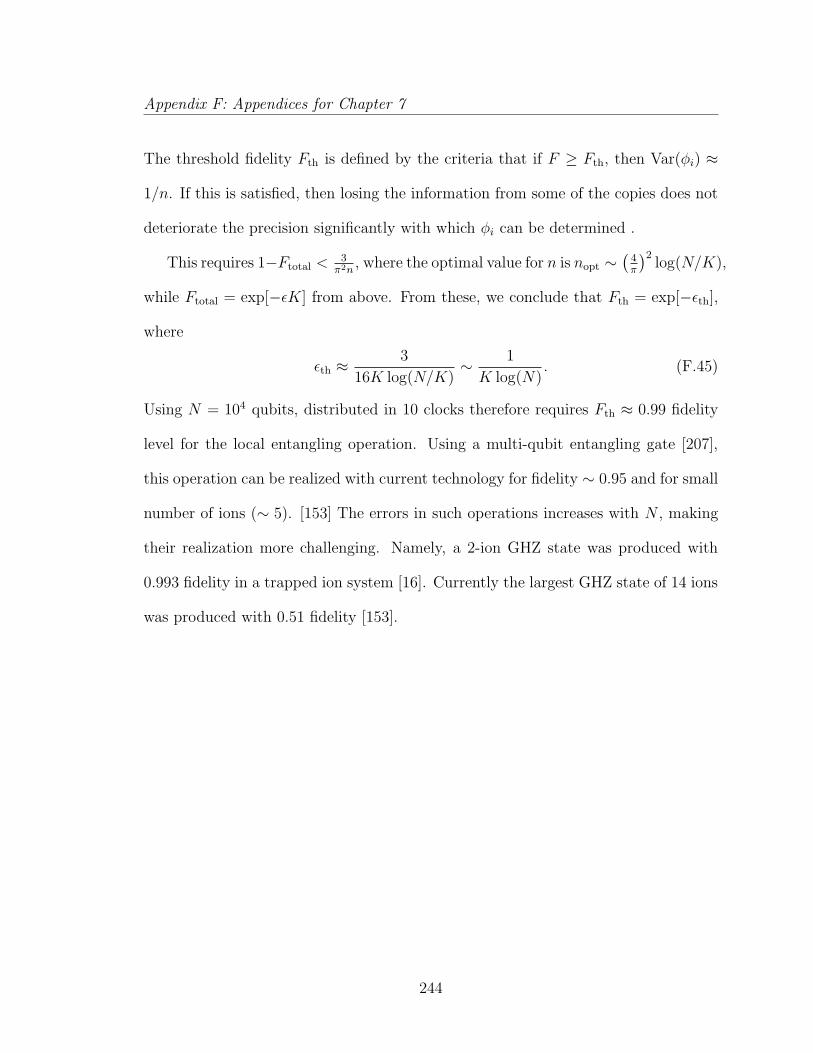
Appendix F: Appendices for Chapter 7
The threshold fidelity Fth is defined by the criteria that if F ≥ Fth, then Var(φi) ≈
1/n. If this is satisfied, then losing the information from some of the copies does not
deteriorate the precision significantly with which φi can be determined .
This requires 1−Ftotal <3π2n
, where the optimal value for n is nopt ∼(
4π
)2log(N/K),
while Ftotal = exp[−εK] from above. From these, we conclude that Fth = exp[−εth],
where
εth ≈3
16K log(N/K)∼ 1
K log(N). (F.45)
Using N = 104 qubits, distributed in 10 clocks therefore requires Fth ≈ 0.99 fidelity
level for the local entangling operation. Using a multi-qubit entangling gate [207],
this operation can be realized with current technology for fidelity ∼ 0.95 and for small
number of ions (∼ 5). [153] The errors in such operations increases with N , making
their realization more challenging. Namely, a 2-ion GHZ state was produced with
0.993 fidelity in a trapped ion system [16]. Currently the largest GHZ state of 14 ions
was produced with 0.51 fidelity [153].
244
Appendix G
Appendices for Chapter 8
G.1 Overview of optimization
In section G.6, we show that the figure of merit, the precision gain with respect
to non-entangled schemes, can be written as
G(N,E) =π
8e−EN
√N
logN, (G.1)
where N is the total number of entangled atoms in the global GHZ state, and E =
E(n,∆,Ω) is the total error (contrast loss) divided by the total number of atoms.
E depends on the number of atoms at a single clock, n, and the detuning (∆) and
Rabi-frequency (Ω) of the dressing field used for local entanglement growing.
We seperate out the minimization of E (through finding the optimal n,∆,Ω pa-
rameters), and the maximization of G (through finding the optimal N). In other
words, we find
Gmax = maxN
G
(N, min
n,∆,ΩE
). (G.2)
245
Appendix G: Appendices for Chapter 8
This two-step procedure gives identical results to the full optimization,
Gmax = maxN,n,∆,Ω
G(N,E(n,∆,Ω)
), (G.3)
bacause both the maximum of G is a monotonically decreasing function of E, for
large Nopt values (as can be read off from Eq. G.1). We choose the two-step precedure
because it is easier to carry out and interpret.
G.2 Local entangling errors
The initial GHZ state is never perfect due to a series of imperfections in the
implementation. Here, we analyze the main errors responsible for lowering the initial
fidelity Flocal = [1 + exp(−εlocal)]/2 of the GHZ state of n atoms, created via the
conditional dressing scheme, described in the main article. We assume the following
errors to be independent and small, and we approximate εlocal with the sum of the
individual errors,∑
j εj. We evaluate the errors for a 2D square lattice filled in a
circular region and a 3D cubic lattice filled in a spherical region (both of radius R).
Where there is a difference between the two cases, we give both results.
G.2.1 Imperfect blockade
If the blockade between the levels r1 and r2, ∆12, is not large enough, the dressing
happens even if r2 is populated by a single atom. Here, we analyze the effect of this
imperfection.
246
Appendix G: Appendices for Chapter 8
The relevant part of the full Hamiltonian of the system during dressing is
H =Ω
2
∑
k
(|r1〉k〈g|k + h.c.) + ∆∑
k
|r1〉k〈r1|k (G.4)
+∑
k
∑
j 6=k
∆j,k|r1〉k〈r1|k|r2〉j〈r2|j, (G.5)
where Ω and ∆ are the Rabi frequency and the detuning of the dressing field,
and ∆j,k = C(3)12 /(~|rj − rk|3) is the shift due to dipole-dipole interaction. Af-
ter adiabatically eliminating the level r1, we can write the effective Hamiltonian as
Heff =∑
kHk|g〉k〈g|k, where
Hk = −Ω2
4∆+∑
j 6=k
(Ω2
4∆− Ω2
4(∆ + ∆j,k)
)|r2〉j〈r2|j, (G.6)
where we also restricted the Hilbert space to at most one r2 excitation.
Ideally, starting from
(|1s〉+ |1r2〉
)(|g〉+ |f〉
)⊗(n−1)
, (G.7)
(where |1x〉 =∑
j |x〉j/√n for x = s, r2), after time t = 4π∆/Ω2, the part of the
wavefunction with no r2 excitation picks up a π phase,
|1s〉(e−iπ|g〉+ |f〉
)⊗(n−1)
, (G.8)
while the part where r2 is present is unchanged, or picks up a small and uniform
phase φ0,
|1r2〉(eiφ0 |g〉+ |f〉
)⊗(n−1)
. (G.9)
In reality, however, dephasing between the different terms of the superposition
occurs. If the system starts from
|Ψ0〉 =1√n
∑
j
|r2〉j⊗
k 6=j
( |g〉k + |f〉k√2
), (G.10)
247

Appendix G: Appendices for Chapter 8
the effective Hamiltonian evolves it into
|Ψt〉 =1√n
∑
j
|r2〉j⊗
k 6=j
(eiφj,k |g〉k + |f〉k√
2
), (G.11)
up to an overall phase, where φj,k = π∆/(∆ + ∆j,k), while the target state is
|Ψtarget〉 =1√n
∑
j
|r2〉j⊗
k 6=j
(eiφ0 |g〉k + |f〉k√
2
), (G.12)
with an appropriately chosen φ0. The fidelity of Ψt with respect to Ψtarget is
F = | 〈Ψtarget|Ψt〉 |2 =
∣∣∣∣∣1
n
∑
j
∏
k 6=j
1 + ei(φj,k−φ0)
2
∣∣∣∣∣
2
. (G.13)
Assuming |φj,k − φ0| 1, and using
1 + eix
2≈ exp
[−x
2
4+ i
x
2
], for x 1 (G.14)
we can write
F =
∣∣∣∣∣1
n
∑
j
(ei
∑k
φj,k−φ02 × e−
∑k
(φj,k−φ0)2
8
)∣∣∣∣∣
2
. (G.15)
We approximate∑
k
(φj,k − φ0)2 ≈ nVar (φj,k) , (G.16)
where the variance is taken over all pairs of (j, k), and we take it out of the summation
to get
F ≈∣∣∣∣∣1
n
∑
j
ei∑k
φj,k−φ02
∣∣∣∣∣
2
e−n4
Var(φj,k). (G.17)
Using the notation, ψj :=∑
k 6=j φj,k, we can write and approximate the first term as
∣∣∣∣∣1
n
∑
j
eiψj/2
∣∣∣∣∣
2
≈ e−14
Var(ψj), (G.18)
where the variance is taken over all j, and we write the total fidelity as
F ≈ exp
[−1
4Var(ψj)−
n
4Var(φj,k)
]=: e−ε1 . (G.19)
248
Appendix G: Appendices for Chapter 8
In section G.8 and section G.9, we evaluate the above variances for a circular 2D
and spherical 3D cloud of radius R, and average density of a−2 and a−3, respectively.
Plugging in the results of Eq. G.101, (G.102) yields
ε1 =1
4[Var(ψj) + nVar(φj,k)] (G.20)
=
(~a3∆
C(3)12
)2
×
0.0209n5 + 0.156n4 (2D)
0.0320n4 + 0.273n3 (3D)
G.2.2 Decaying Rydberg states
During dressing, there is an average number of n(Ω/(2∆))2 Rydberg excitations
present at level r1 in the ensemble. Any decay or dephasing of r1 Rydberg state then
results in the loss of fidelity,
ε2 ≈ γ1t× n(
Ω
2∆
)2
= πnγ1
∆, (G.21)
where γ1 is the total rate of loss (environment induced decay and dephasing) from
the Rydberg level r1, and t is assumed to take the optimal value, t = 4π∆/Ω2.
In the same time, in the other part of the wavefunction, there is exactly one r2
excitation. If this decays and dephases with rate γ2, then the fidelity error due to
this is
ε3 ≈ γ2t = 4π∆γ2
Ω2, (G.22)
where, again, we used that t = 4π∆/Ω2.
G.2.3 Rydberg interaction induced broadening
Although the Rydberg-Rydberg interaction is assumed to be strong, which makes
single-to-double excitations off-resonant, the external laser field can easily drive Ra-
249

Appendix G: Appendices for Chapter 8
man transitions between different single excitations states. Let us define the following
states
|j〉 := σ†j |gg . . . g〉, where σ†j = |r1〉j〈g|j, (G.23)
|S〉 :=1√n
∑
j
|j〉, (G.24)
|j, k〉 := σ†jσ†k|gg . . . g〉 = σ†j |k〉 = σ†k|j〉, for j < k, (G.25)
for j, k ∈ 1, 2 . . . n, indexing the atoms in the ensemble.
The full Hamiltonian of the system during the dressing is Hfull =∑n
j=1 Hj, where
Hj = ∆σ†jσj +Ω
2
(|r1〉j〈g|j + h.c.
)
+∑
k>j
∆j,kσ†jσjσ
†kσk. (G.26)
It contains a Rydberg-Rydberg interaction term, whose strength, ∆j,k = ∆rr(|rj−rk|)
depends on the distance between atoms j and k. In the subspace of single and double
excitations, Span|j〉, |j, k〉, Hj is equivalent to
∑
k>j
(∆ + ∆j,k)|j, k〉〈j, k|+Ω
2
∑
k>j
(|j〉〈j, k|+ h.c.
), (G.27)
which is partially depicted on Fig. G.1.
If all Rydberg shifts are large compared to√nΩ, then the double excitation prob-
ability is small, and the dynamics is well described by the following effective Hamil-
tonian, Heff =∑
j Heff,j, where
Heff,j = ∆j|j〉〈j|+∑
k>j
Ωj,k
2
(|j〉〈k|+ h.c.
), (G.28)
where ∆j = −∑k 6=jΩ2
4(∆j,k+∆), and Ωj,k = − Ω2
2(∆j,k+∆).
250
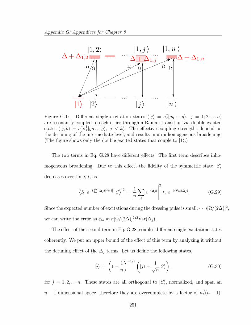
Appendix G: Appendices for Chapter 8
Figure G.1: Different single excitation states (|j〉 = σ†j |gg . . . g〉, j = 1, 2, . . . n)are resonantly coupled to each other through a Raman-transition via double excitedstates (|j, k〉 = σ†jσ
†k|gg . . . g〉, j < k). The effective coupling strengths depend on
the detuning of the intermediate level, and results in an inhomogeneous broadening.(The figure shows only the double excited states that couple to |1〉.)
The two terms in Eq. G.28 have different effects. The first term describes inho-
mogeneous broadening. Due to this effect, the fidelity of the symmetric state |S〉
decreases over time, t, as
∣∣⟨S∣∣e−i
∑j ∆jt|j〉〈j|
∣∣S⟩∣∣2 =
∣∣∣∣∣1
n
∑
j
e−i∆jt
∣∣∣∣∣
2
≈ e−t2Var(∆j). (G.29)
Since the expected number of excitations during the dressing pulse is small, ∼ n[Ω/(2∆)]2,
we can write the error as ε4a ≈ n[Ω/(2∆)]2t2Var(∆j).
The effect of the second term in Eq. G.28, couples different single-excitation states
coherently. We put an upper bound of the effect of this term by analyzing it without
the detuning effect of the ∆j terms. Let us define the following states,
|j〉 :=
(1− 1
n
)−1/2(|j〉 − 1√
n|S〉), (G.30)
for j = 1, 2, . . . n. These states are all orthogonal to |S〉, normalized, and span an
n − 1 dimensional space, therefore they are overcomplete by a factor of n/(n − 1),
251
Appendix G: Appendices for Chapter 8
and they are also almost orthogonal to each other:∣∣∣⟨j|k⟩∣∣∣ = 1
n+ 1
n2 = O(1/n). Let
us imagine starting the system in |S〉, and observing the probability accumulating
in all the other states |j〉. The time evolution of the amplitudes, cj, dictated by the
Heisenberg equations, can be approximated as
d
dtcj(t) = −i
⟨j|Heff,Ω|S
⟩cs(t) +O(ck(t))
≈ −i⟨j|Heff,Ω|S
⟩cs(0),
cj(t) ≈ −it⟨j|Heff,Ω|S
⟩cs(0), (G.31)
where, |cs(0)|2 ≈ n(Ω/(2∆))2, and Heff,Ω =∑
j,k>j Ωj,k(|j〉〈k|+h.c.). The conditional
probability accumulating in |j〉 is
Pj(t)
|cs(0)|2 ≈ t2∣∣⟨j|Heff,Ω|S
⟩∣∣2
≈ t2
∣∣∣∣∣∑
k
1√n
(Ωj,k
2− 1
n
∑
l
Ωl,k
2
)∣∣∣∣∣
2
= t21
n
∣∣∣∣∣∆j −1
n
∑
l
∆l
∣∣∣∣∣
2
, (G.32)
where we used that∑
k 6=j Ωj,k/2 = ∆j. The total conditional probability of leaving
the symmetric state |S〉 is
P (t)
|cS(0)|2 ≈ t21
n
∑
j
∣∣∣∣∣∆j −1
n
∑
l
∆l
∣∣∣∣∣
2
= t2Var(∆j), (G.33)
and the total error is ε4b = P (t) = n[Ω/(2∆)]2t2Var(∆j). This is identical to the
error originating from the ∆jk term of Eq. G.28. We approximate the effect of these
two errors by adding them, giving
ε4a + ε4b =n
2
(Ω
∆
)2
t2 Var(∆j). (G.34)
252
Appendix G: Appendices for Chapter 8
We evaluate the variance of ∆j in section G.10 for both the 2D and the 3D case.
The result is given in Eq. G.126 and (G.127). Plugging the result in, and using that
t = 4π∆/Ω2, we can write the error as
ε4 ≈ ε4a + ε4b =
0.0312n9
(~a6Ω
C(6)11
)2
(2D)
0.172n7
(~a6Ω
C(6)11
)2
(3D)
(G.35)
where a is the lattice constant of the 2D (3D) optical lattice holding the atoms, and
C(6)11 is the coefficient of the van der Waals interaction between two atoms excited to
r1 level.
G.3 Non-local entangling errors
Our protocol requires K − 1 links to be set up between K clocks. We denote
the fidelity of a single connection by Fnon−local = [1 + exp(−εnon−local)]/2, and we
approximate εnon−local with the sum of individual errors∑
i εi, detailed below.
G.3.1 Imperfect blockade
When exciting a single collective excitation, imperfect self-blockade can result
in leakage into double excited states. The probability of this can be exponentially
reduced by applying a smooth driving pulse. E.g., in case of a Gaussian pulse of
width τ , and area π, exciting the g → r1 transition is expected to be blocked when
r2 is populated, but it succeeds with probability Pdouble,
Pdouble ≈π2
4exp
[−(∆12τ)2
2
], (G.36)
253
Appendix G: Appendices for Chapter 8
where ∆12 = C(3)12 /(~(2R)3) is the minimal energy shift in the ensemble due to the
interaction of two atoms, one in r1 and one in r2. A detailed analysis of how different
pulses affect the transition probability can be found in [55]. Pdouble 1 requires
τ ≤√
2
∆12
=
2n3/2 ~a3
C(3)12
(2D)
2.7n ~a3
C(3)12
(3D)
(G.37)
in order to be small compared to the other errors.
G.3.2 Rydberg state decay
The g → r1 transition is driven with a pulse of duration τ , during which the r2 level
has a single excitation, which decays with rate γ2. The resulting error contribution,
after all four photon pulses have been generated, is
ε5 = 4γ1τ =
8n3/2 ~a3γ1
C(3)12
(2D)
10.8n~a3γ1
C(3)12
(3D)
(G.38)
where we used the expressions for τ from Eq. G.37.
G.3.3 Photon propagation and detection errors
The pairs of photons can get lost in the fiber during propagation and the detection
process (which is limited to 50% for time-resolving detectors, and 25% for non-time-
resolving ones). The two-photon heralding, however, detects both of these errors.
The remaining error comes from dark-counts of the detectors. This affects a single
link with the error
ε6 ≈ 4γdarkTdetect = γdark20
nγe, (G.39)
254

Appendix G: Appendices for Chapter 8
where γdark is the dark count rate of the detectors, Tdetect (chosen such that a properly
timed detector would have a chance to catch 1 − e−5 > 99% of each photon) is
the “open time” of the detector, and γe is the spontaneous emission lifetime of the
|e〉 → |f〉 transitions. The factor of n is due to the bosonic enhancement of the said
transition, and the factor of 4 is because four pulses are used in each connection.
G.3.4 Memory loss
During the creation step of each link, the state |s〉 is used as memory. On average,
every link relies on one s qubit. The time it takes to attempt the creation of a
link is ∼ 2L/c, the time it takes for a light pulse to do a round-trip between two
stations. During this time, quantum information is stored in qubit s, which is subject
to decoherence happening at a rate γs. The infidelity of the link originating from this
error is
ε7 = 42L
cγs. (G.40)
State |f〉 is assumed to be a long-lived clock state, its decoherence rate is negligible.
G.3.5 Imperfect branching ratios
Bosonic enhancement makes the excited atom in state |e〉 decay preferentially
to |g〉, and emit a photon directly to the spatial mode ke, where ke is the spatial
frequency of the collective mode e. However, in the implementation with Yb atoms
(discussed in Section G.4), the decay channel to |g〉 has a branching ratio of ζ = 0.64.
255
Appendix G: Appendices for Chapter 8
The total probability of decay through all other channels is
ε8 = 4γnot f
γtot
≈ 41− ζ
nζ + 1− ζ ∼2
n, (G.41)
where n ( 1) is the number of atoms in a single ensemble.
G.4 Implementation with Yb
We imagine using the lower levels of neutral Yb for our protocol, |g〉 = |6s6p(3P0)〉,
|f〉 = |6s2(1S0)〉, |s〉 = |6s6p(3P2)〉 and |e〉 = |5d6s(3D1)〉, and two Rydberg levels
|r1〉 = |6sns(1S0)〉 and |r2〉 = |6snpm=+1(1P1)〉 with the same principle quantum
number n for high-energy state. In the case of the 2D lattice, we set the quantization
axis perpendicular to the plane in which the atoms reside, this way the dipole-dipole
interaction between two atoms, one in |r2〉 and the other in |r1〉, depends only on
their separation, |r1− r2|. In the case of the 3D lattice, we rely on the overwhelming
strength of the Rydberg interaction to produce reliable blockade even between atoms
in different horizontal planes.
G.4.1 Rydberg lifetimes
We use the measured values from [83], and extrapolate the inverse lifetimes of the
Rydberg states
γ1 ≈ γ2 = γ =8.403× 10⁸ Hz
(n− 4.279)3(G.42)
where n is the principle quantum number of the Rydberg orbit. Although the mea-
surement was carried out at 300 K, the contribution of the black body radiation
is negligible even at this temperature. Furthermore, the photoionization rate in a
256

Appendix G: Appendices for Chapter 8
trapping field with 104 W/cm2 intensity is also more than one order of magnitude
smaller.
G.4.2 Self-blockade, ∆11
The long-range interaction between two r1 atoms at a distance R is dominated by
the van der Waals potential,
∆11(R) =C
(6)11
~R6, (G.43)
where C(6)11 strongly depends on the principle quantum number n. We use results from
[222], and extrapolate the C(6)11 coefficient to high principle quantum numbers with
the following formula,
C(6)11 = (−0.116 + 0.0339 n) n11 a.u. (G.44)
where the a.u. stands for atomic units, Eha60 = 9.573 × 10−80 Jm6, where Eh is the
Hartree energy and a0 is the Bohr radius.
G.4.3 Cross-blockade, ∆12
The long-range interaction between an r1 and an r2 atoms at a distance R is
dominated by the dipole-dipole interaction. We assume that the atoms are confined
in the xy plane, and because the 6snpm=+1 state is polarized in the z direction, the
interaction strength is independent of the relative direction of one atom to the other.
∆12(R) =C
(3)12
~R3, (G.45)
where C(3)12 depends strongly on the principle quantum number n. We use results from
[222], and extrapolate the C(3)12 coefficient to high principle quantum numbers with
257
Appendix G: Appendices for Chapter 8
the following formula,
C(3)12 = (0.149 + 0.00077 n) n4 a.u. (G.46)
where the a.u. stands for atomic units, Eha30 = 6.460× 10−49 Jm3.
G.4.4 Decay rates of lower levels
The decay rate of |s〉 = |6s6p , 3P2〉 is γs = [14.5 s]−1 = 0.069 Hz. The decay rate
of the excited state |e〉 = |5d6s , 3D1〉 is γe = [380 ns]−1 = 2.63× 10⁶ Hz.
G.4.5 Photon channels
We assume that neighboring stations are L < 10 km apart from each other, we
neglect fiber and coupling loss. We further assume that single photon detectors have
a low dark count rate, i.e. γdark ≈ 10 Hz.
G.5 Optimization
The total initial imperfections of a GHZ state with N atoms divided into K = N/n
groups, each containing n atoms, is
εtot = (K − 1)εnon−local +Kεlocal ≈ −N
n
∑
i
εi, (G.47)
where the error contributions are from Eq. (G.20, G.21, G.22, G.35, G.38, G.39, G.40,
and G.41). Independently from the total atom number, N , there is an optimal group
size, nopt, for which∑
i εi/n is minimal. If the total number of atoms is increased, it
is best to create multiple groups of the same size. Below, we find the optimal values of
258
Appendix G: Appendices for Chapter 8
the parameters Ω, ∆ (the Rabi frequency and the detuning of the dressing field), and
n (the size of the local groups) for fixed values of n (the principle quantum number
of the Rydberg state) and a = 275.75 nm.
Using the following dimensionless variables, ω = Ω/γ, δ = ∆/γ, δ11 =C
(6)11
~a6γand
δ12 =C
(3)12
~a3γ, we can write the error per atom as E :=
∑i εi/n =
∑i ei, where the terms
are
e1 =
(δ
δ12
)2
×
0.021n4 + 0.16n3 (2D)
0.032n3 + 0.27n2 (3D)
(G.48)
e2 =π
δ(G.49)
e3 =4π
n
δ
ω2(G.50)
e4 =
(ω
δ11
)2
×
0.031n8 (2D)
0.17n6 (3D)
(G.51)
e5 =1
δ12
×
8n1/2 (2D)
10.8 (3D)
(G.52)
e6 = 7.6× 10⁻⁵ 1
n2(G.53)
e7 = 1.8× 10⁻⁵ 1
n(G.54)
e8 =2
n2(G.55)
G.5.1 Optimal parameters
We numerically minimized the sum, E =∑
i ei, by finding the optimal values of
ω, δ and n for every n ∈ [50, 150]. The optimal driving strength ωopt, the optimal
detuning for the dressing field δopt, and the optimal number of atoms at a single clock
nopt are shown on Fig. G.2.
259
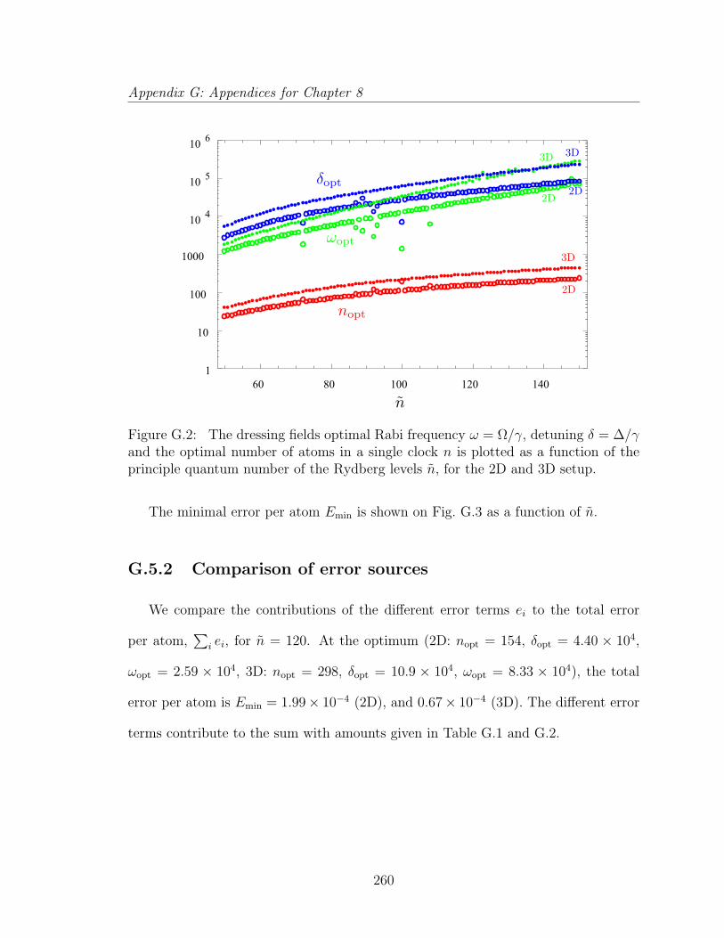
Appendix G: Appendices for Chapter 8
Figure G.2: The dressing fields optimal Rabi frequency ω = Ω/γ, detuning δ = ∆/γand the optimal number of atoms in a single clock n is plotted as a function of theprinciple quantum number of the Rydberg levels n, for the 2D and 3D setup.
The minimal error per atom Emin is shown on Fig. G.3 as a function of n.
G.5.2 Comparison of error sources
We compare the contributions of the different error terms ei to the total error
per atom,∑
i ei, for n = 120. At the optimum (2D: nopt = 154, δopt = 4.40 × 10⁴,
ωopt = 2.59 × 10⁴, 3D: nopt = 298, δopt = 10.9 × 10⁴, ωopt = 8.33 × 10⁴), the total
error per atom is Emin = 1.99× 10⁻⁴ (2D), and 0.67× 10⁻⁴ (3D). The different error
terms contribute to the sum with amounts given in Table G.1 and G.2.
260

Appendix G: Appendices for Chapter 8
Errors in 2D ensemble error per atom ratio in total
imperfect blockade (e1) 3.30× 10⁻⁵ 17%
r1 decay (e2) 7.14× 10⁻⁵ 36%
r2 decay (e3) 5.36× 10⁻⁶ 3%
inhom. broadening (e4) 5.36× 10⁻⁶ 3%
r2 decay (non-local) (e5) ∼ 10−9 < 0.1%
photon detection (e6) ∼ 10−9 < 0.1%
memory error (e7) ∼ 10−7 < 0.1%
imperfect br. ratios (e8) 8.40× 10⁻⁵ 42%
total error per atom 1.99× 10⁻⁴ 100%
Table G.1: The absolute and relative contribution of the different error sources tothe total error per atom at n = 120, ∆ = ∆opt = 4.40×10⁴ γ, Ω = Ωopt = 2.59×10⁴ γand n = nopt = 154.
261
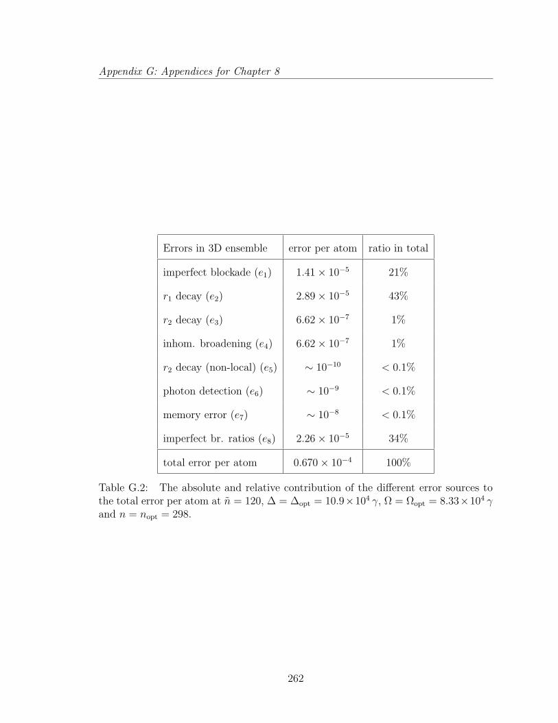
Appendix G: Appendices for Chapter 8
Errors in 3D ensemble error per atom ratio in total
imperfect blockade (e1) 1.41× 10⁻⁵ 21%
r1 decay (e2) 2.89× 10⁻⁵ 43%
r2 decay (e3) 6.62× 10⁻⁷ 1%
inhom. broadening (e4) 6.62× 10⁻⁷ 1%
r2 decay (non-local) (e5) ∼ 10−10 < 0.1%
photon detection (e6) ∼ 10−9 < 0.1%
memory error (e7) ∼ 10−8 < 0.1%
imperfect br. ratios (e8) 2.26× 10⁻⁵ 34%
total error per atom 0.670× 10⁻⁴ 100%
Table G.2: The absolute and relative contribution of the different error sources tothe total error per atom at n = 120, ∆ = ∆opt = 10.9×10⁴ γ, Ω = Ωopt = 8.33×10⁴ γand n = nopt = 298.
262
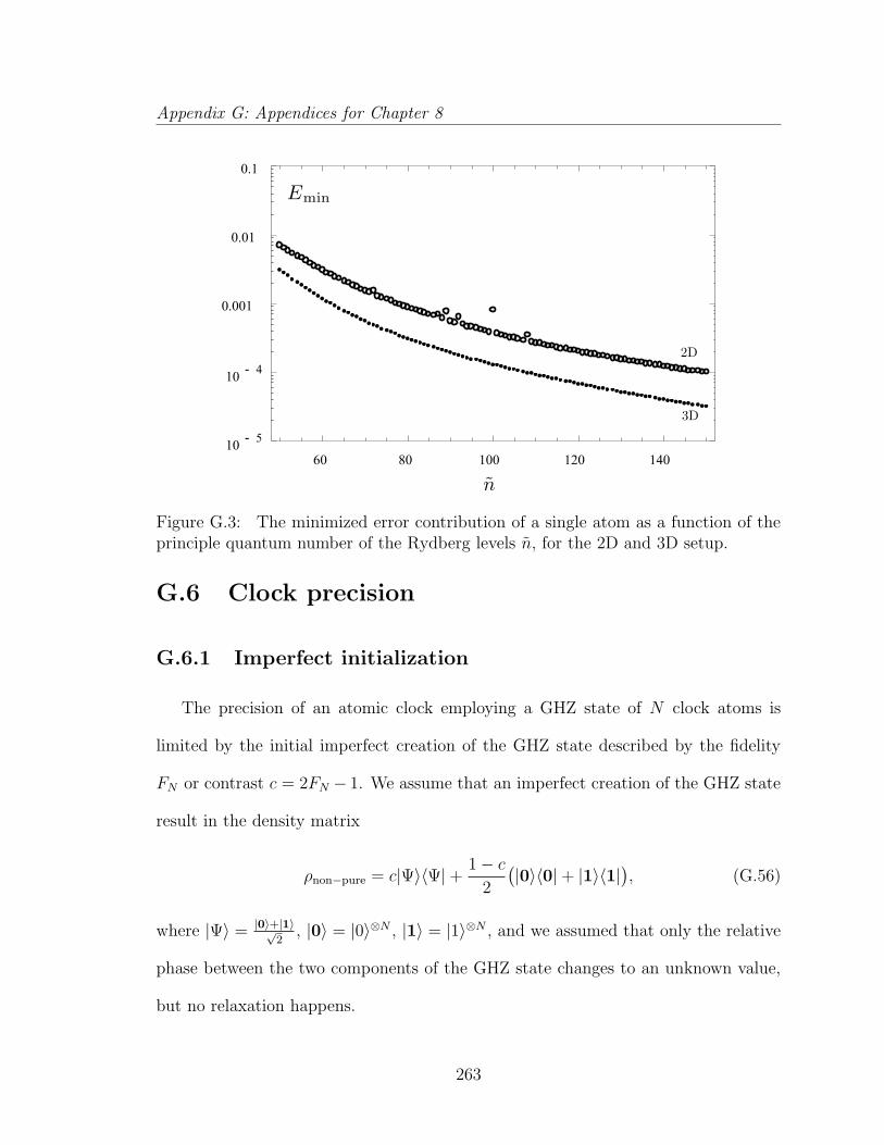
Appendix G: Appendices for Chapter 8
Figure G.3: The minimized error contribution of a single atom as a function of theprinciple quantum number of the Rydberg levels n, for the 2D and 3D setup.
G.6 Clock precision
G.6.1 Imperfect initialization
The precision of an atomic clock employing a GHZ state of N clock atoms is
limited by the initial imperfect creation of the GHZ state described by the fidelity
FN or contrast c = 2FN − 1. We assume that an imperfect creation of the GHZ state
result in the density matrix
ρnon−pure = c|Ψ〉〈Ψ|+ 1− c2
(|0〉〈0|+ |1〉〈1|
), (G.56)
where |Ψ〉 = |0〉+|1〉√2
, |0〉 = |0〉⊗N , |1〉 = |1〉⊗N , and we assumed that only the relative
phase between the two components of the GHZ state changes to an unknown value,
but no relaxation happens.
263
Appendix G: Appendices for Chapter 8
G.6.2 Measurement
After the interrogation time, the two components of the GHZ state pick up a
relative phase Nφ. |Ψ〉 → |Ψφ〉 = [|0〉 + eiNφ|1〉]/√
2. Performing a perfect single-
atom −π/2 rotation around the y axis for all atoms transforms this into
|Ψ′φ〉 =1√
2N+1
∑
qj
[1 + (−1)
∑j qjeiNφ
]|q1, q2, . . . qN〉, (G.57)
where qj ∈ 0, 1 stands for the state of atom j. After this, we measure every atom (in
the z-basis). The probability of any resulting sequence, q = (q1, q2, . . . qN) ∈ 0, 1×N ,
is
P(q|Ψ′φ) =1
2N+1
[1 + (−1)
∑j qj cos(Nφ)
], (G.58)
and the probability of the parity, p =(∑
j qj)mod2, is
P(p|Ψ′φ) =1 + (−1)p cos(Nφ)
2, p ∈ 0, 1. (G.59)
On the other hand, these probabilities are different when they are conditioned on
being in the mixed part of the density matrix.
P(q|ρmixed) =1
2N, P(p|ρmixed) =
1
2(G.60)
∀q ∈ 0, 1×N and ∀p ∈ 0, 1, where ρmixed = [|0〉〈0|+ |1〉〈1|]/2.
The resulting total probability is the weighted sum of the two cases,
P(p|φ) = cP(p|Ψ′φ) + (1− c)P(p|ρmixed) (G.61)
=1 + c(−1)p cos(Nφ)
2, (G.62)
where c = 2FN − 1 is the contrast of the interference fringes.
264

Appendix G: Appendices for Chapter 8
G.6.3 Fisher information
We rely on inferring the unknown phase φ, from a series of parity measurements,
as described above. The information content (about φ) of a single measured value p
is quantified by the Fisher information,
F(φ) =∑
p∈0,1
P(p|φ)
[ln
d
dφP(p|φ)
]2
(G.63)
= N2 sin2(Nφ)
1/c2 − cos2(Nφ), (G.64)
where the true value of the phase is φ. The average Fisher information is
F =1
2π
+π∫
−π
dφF(φ), (G.65)
which we can evaluate in the limit of c 1,
F ≈ 1
2π
∫dφ c2 cos2(Nφ) =
N2c2
2. (G.66)
In the other limit, when 1− c 1, F (φ) is approximately c2 everywhere, except near
the points where sin(Nφ) = 0. We approximate the dip at φ = 0 with
sin2 x
1/c2 − cos2 x≈ x2
1−c2c2
+ x2, where x = Nφ, (G.67)
and the integral with
FN2
≈ c2 − 2
2π
∫ +π
−πdx
(1− x2
1−c2c2
+ x2
)(G.68)
= c2 −√
1− c2
c≈ 1−
√2(1− c), (G.69)
where we have used that F is periodic with period 2π/N .
265
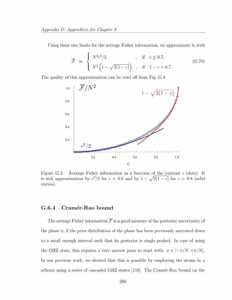
Appendix G: Appendices for Chapter 8
Using these two limits for the average Fisher information, we approximate it with
F ≈
N2c2/2 , if c ≤ 0.7,
N2(
1−√
2(1− c))
, if 1− c > 0.7.
(G.70)
The quality of this approximation can be read off from Fig. G.4
Figure G.4: Average Fisher information as a function of the contrast c (dots). Itis well approximation by c2/2 for c < 0.6 and by 1 −
√2(1− c) for c > 0.8 (solid
curves).
G.6.4 Cramer-Rao bound
The average Fisher information F is a good measure of the posterior uncertainty of
the phase φ, if the prior distribution of the phase has been previously narrowed down
to a small enough interval such that its posterior is single peaked. In case of using
the GHZ state, this requires a very narrow prior to start with: φ ∈ [−π/N,+π/N ].
In our previous work, we showed that this is possible by employing the atoms in a
scheme using a series of cascaded GHZ states [116]. The Cramer-Rao bound on the
266
Appendix G: Appendices for Chapter 8
expected deviation of the estimated φ from the true one implies
∆φ =√〈(φestimate − φtrue)2〉 ≥
[νF]−1/2
, (G.71)
where ν is the number of independent repetitions of the measurement. We are going
to assume equality to simplify our analysis.
G.6.5 Allan-deviation
The average fractional frequency uncertainty of an atomic clock (with central
frequency ω0), averaged over a long time period τ , is called Allan-deviation [116],
σ =(∆ω)τω0
≈ ∆φt/t
ω0
1√τ/t≈ 1
ω0
√τ
[νtF
]−1/2(G.72)
where (∆ω)τ =∣∣ 1τ
∫dτ ′ ω(τ ′)− ω0
∣∣ is the deviation of the average frequency over
time τ , and ∆φt is the average deviation of the measured phase (from the true one)
in a single interrogation of length t. The√τ/t factor comes from the number of
independent repetitions of the same, t-long, interrogation cycle.
In Ref. [121], we showed that σ can reach
σent ≈1
ω0τ
8
π
√logN
N, (G.73)
if τ < γ−1at /N , the reduced atomic coherence time, and if the contrast is perfect, (c =
1). Using the approximation for F ≈ N2c2/2, and the fact that σ ∝ [F ]−1/2 ∝ c−1,
we can augment this result with a c-dependence, and express the Allan-deviation in
the presence of imperfections as
σ(imperfect)ent = σent/c =
1
cω0τ
8
π
√logN
N. (G.74)
267
Appendix G: Appendices for Chapter 8
G.6.6 Comparison to non-entangled interrogation
Using the same number of atoms, N , we can arrange a measurement without using
any entanglement. This results in the Allan-deviation of
σnon−ent(τ) ≈ 1
ω0τ√N, if τ < 1/γLO, (G.75)
where γ−1LO is the laser coherence time. This, representing the standard quantum limit
(SQL), is expected to be larger than the Allan-deviation corresponding to the GHZ
state scheme, which is almost at the Heisenberg limit. The precision gain of the GHZ
scheme over the non-entangled one is
G =σnon−ent
σent/c= (2FN − 1)
π
8
√N
logN. (G.76)
Since the fidelity FN decreases with increasing N , there exist an optimal Nopt, for
which the gain G is maximal.
G.6.7 Optimal clock network size
If each clock runs with the optimal setup (δopt, ωopt, nopt), then the total error per
atom, E, is minimal, and the total fidelity can be written as FN =[1 + e−EminN
]/2.
Plugging this into Eq. G.76 gives
G = e−EminNπ
8
√N
logN, (G.77)
which takes its maximum atN = Nmax ≈ 12Emin
, givingGmax ≈ π8
[Emin log
(1
2Emin
)]−1/2
.
In the meantime the number of atoms at a single clock is given by nopt. As a result
the optimal number of clocks becomes
Kopt ≤Nmax
nopt
≈ 1
2Eminnopt
. (G.78)
268
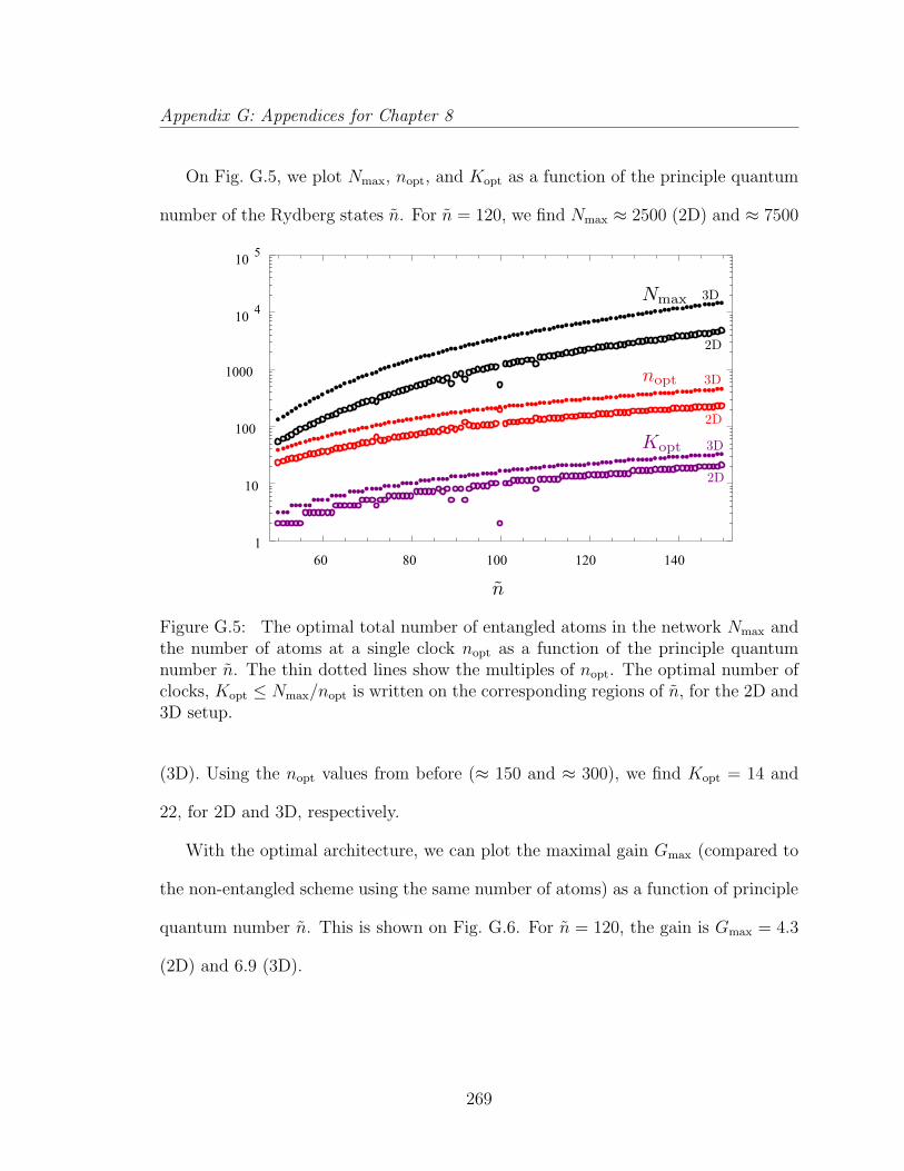
Appendix G: Appendices for Chapter 8
On Fig. G.5, we plot Nmax, nopt, and Kopt as a function of the principle quantum
number of the Rydberg states n. For n = 120, we find Nmax ≈ 2500 (2D) and ≈ 7500
Figure G.5: The optimal total number of entangled atoms in the network Nmax andthe number of atoms at a single clock nopt as a function of the principle quantumnumber n. The thin dotted lines show the multiples of nopt. The optimal number ofclocks, Kopt ≤ Nmax/nopt is written on the corresponding regions of n, for the 2D and3D setup.
(3D). Using the nopt values from before (≈ 150 and ≈ 300), we find Kopt = 14 and
22, for 2D and 3D, respectively.
With the optimal architecture, we can plot the maximal gain Gmax (compared to
the non-entangled scheme using the same number of atoms) as a function of principle
quantum number n. This is shown on Fig. G.6. For n = 120, the gain is Gmax = 4.3
(2D) and 6.9 (3D).
269
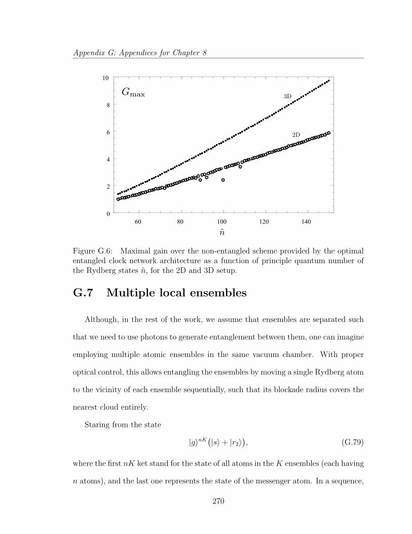
Appendix G: Appendices for Chapter 8
Figure G.6: Maximal gain over the non-entangled scheme provided by the optimalentangled clock network architecture as a function of principle quantum number ofthe Rydberg states n, for the 2D and 3D setup.
G.7 Multiple local ensembles
Although, in the rest of the work, we assume that ensembles are separated such
that we need to use photons to generate entanglement between them, one can imagine
employing multiple atomic ensembles in the same vacuum chamber. With proper
optical control, this allows entangling the ensembles by moving a single Rydberg atom
to the vicinity of each ensemble sequentially, such that its blockade radius covers the
nearest cloud entirely.
Staring from the state
|g〉nK(|s〉+ |r2〉
), (G.79)
where the first nK ket stand for the state of all atoms in the K ensembles (each having
n atoms), and the last one represents the state of the messenger atom. In a sequence,
270
Appendix G: Appendices for Chapter 8
we imagine the messenger atom to be brought to the vicinity of each ensemble, and
the pulse sequence [π/2]g,f , [π(∆)]f,r1, [π/2]g,f (where [π(∆)]f,r1 is the same dressing
field as described in the main text), performs a collective flip conditioned on the state
of the messenger atom. This plays out as follows
→ |g〉n(K−1)(|f〉n|s〉+ |g〉n|r2〉
)(G.80)
→ |g〉n(K−2)(|f〉2n|s〉+ |g〉2n|r2〉
)(G.81)
... (G.82)
→(|f〉Kn|s〉+ |g〉Kn|r2〉
), (G.83)
which then only requires the messenger atom to be measured in the |±〉 = (|s〉± |r2〉)
basis, resulting in
→ |f〉Kn ± |g〉Kn, (G.84)
the global GHZ state.
Disregarding the technical difficulties of trapping multiple atomic ensembles in
the same vacuum chamber, this entangling method has a higher fidelity than the pre-
vious protocol, since it does not suffer from the errors affecting the photon emission,
propagation and detection. We model the imperfections of this scheme by summing
the error terms ε1 + ε2 + ε3 + ε4 (from Eq. (G.20), (G.21), (G.22), (G.35)).
If the different ensembles are stored in different parts of a 3D lattice, and we
disregard the errors that can occur during the transport of the messenger atom, then
we can optimize the total error per atom E = e1 + e2 + e3 + e4. Without constraints
this would suggest n = 1 (i.e. each ensemble containing a single atom), and very high
Ω and ∆ values. Instead of this unrealistic result, we optimize E for a fixed n = 100,
271
Appendix G: Appendices for Chapter 8
which is a realistic number of atoms that can fit inside the blockade radius in current
atomic lattice clocks.
For principle quantum number n = 120 and for fixed n = 100, we find ω =
4.4× 10⁵, δ = 3.1× 10⁵ and Emin = 1.49× 10⁻⁵, which translates to Gmax = 13.5 for
Nmax = 3 × 10⁴ and Kopt ≈ 300. This means that if we can employ enough atoms
in a single clock, than the overall gain factor G can be improved by a factor of 2,
compared to the network realization.
G.8 Calculating Var(φj,k)
Here, we calculate the variance of
φj,k =π∆
∆ + ∆j,k
≈ π∆
∆j,k
=π~∆
C(3)12
|rj − rk|3, (G.85)
where we assume ∆j,k ∆ for all (j, k) pairs, over an ensemble of n atoms, trapped in
a (square or cubic)lattice with periodicity a, uniformly filling a circular 2D (spherical
3D) region of radius R.
G.8.1 Calculating 〈φj,k〉
Averaging over the cloud of atoms,
〈φj,k〉 =π~∆
C(3)12
⟨|rj − rk|3
⟩, (G.86)
can be approximated by the following integral
≈ π~∆
C(3)12
1
V 2
∫
V
dηrj
∫
V
dηrk |rj − rj|3 =~R3∆
C(3)12
J1, (G.87)
272
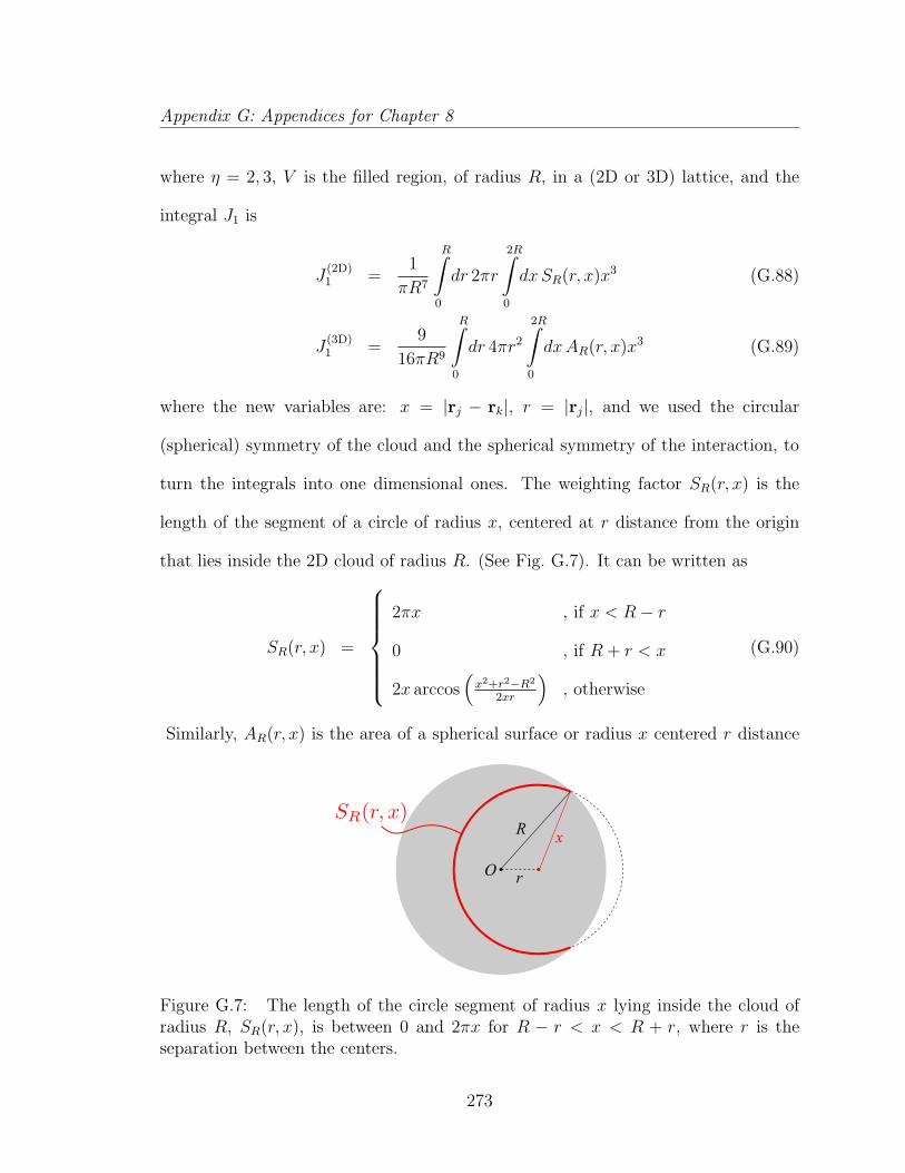
Appendix G: Appendices for Chapter 8
where η = 2, 3, V is the filled region, of radius R, in a (2D or 3D) lattice, and the
integral J1 is
J(2D)1 =
1
πR7
R∫
0
dr 2πr
2R∫
0
dxSR(r, x)x3 (G.88)
J(3D)1 =
9
16πR9
R∫
0
dr 4πr2
2R∫
0
dxAR(r, x)x3 (G.89)
where the new variables are: x = |rj − rk|, r = |rj|, and we used the circular
(spherical) symmetry of the cloud and the spherical symmetry of the interaction, to
turn the integrals into one dimensional ones. The weighting factor SR(r, x) is the
length of the segment of a circle of radius x, centered at r distance from the origin
that lies inside the 2D cloud of radius R. (See Fig. G.7). It can be written as
SR(r, x) =
2πx , if x < R− r
0 , if R + r < x
2x arccos(x2+r2−R2
2xr
), otherwise
(G.90)
Similarly, AR(r, x) is the area of a spherical surface or radius x centered r distance
Figure G.7: The length of the circle segment of radius x lying inside the cloud ofradius R, SR(r, x), is between 0 and 2πx for R − r < x < R + r, where r is theseparation between the centers.
273
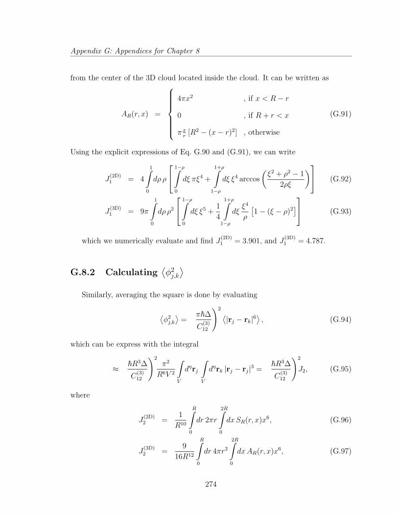
Appendix G: Appendices for Chapter 8
from the center of the 3D cloud located inside the cloud. It can be written as
AR(r, x) =
4πx2 , if x < R− r
0 , if R + r < x
π xr
[R2 − (x− r)2] , otherwise
(G.91)
Using the explicit expressions of Eq. G.90 and (G.91), we can write
J(2D)1 = 4
1∫
0
dρ ρ
1−ρ∫
0
dξ πξ4 +
1+ρ∫
1−ρ
dξ ξ4 arccos
(ξ2 + ρ2 − 1
2ρξ
) (G.92)
J(3D)1 = 9π
1∫
0
dρ ρ2
1−ρ∫
0
dξ ξ5 +1
4
1+ρ∫
1−ρ
dξξ4
ρ
[1− (ξ − ρ)2
] (G.93)
which we numerically evaluate and find J(2D)1 = 3.901, and J
(3D)1 = 4.787.
G.8.2 Calculating⟨φ2j,k
⟩
Similarly, averaging the square is done by evaluating
⟨φ2j,k
⟩=
(π~∆
C(3)12
)2 ⟨|rj − rk|6
⟩, (G.94)
which can be express with the integral
≈(~R3∆
C(3)12
)2π2
R6V 2
∫
V
dηrj
∫
V
dηrk |rj − rj|3 =
(~R3∆
C(3)12
)2
J2, (G.95)
where
J(2D)2 =
1
R10
R∫
0
dr 2πr
2R∫
0
dxSR(r, x)x6, (G.96)
J(3D)2 =
9
16R12
R∫
0
dr 4πr2
2R∫
0
dxAR(r, x)x6, (G.97)
274
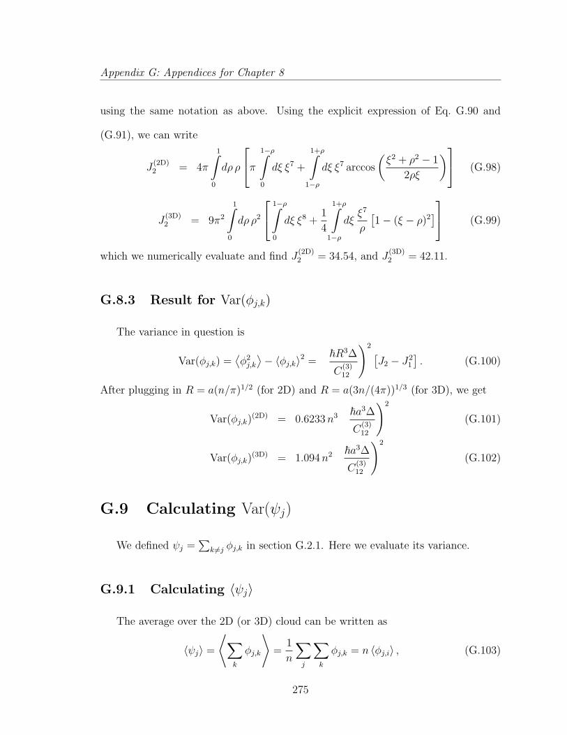
Appendix G: Appendices for Chapter 8
using the same notation as above. Using the explicit expression of Eq. G.90 and
(G.91), we can write
J(2D)2 = 4π
1∫
0
dρ ρ
π
1−ρ∫
0
dξ ξ7 +
1+ρ∫
1−ρ
dξ ξ7 arccos
(ξ2 + ρ2 − 1
2ρξ
) (G.98)
J(3D)2 = 9π2
1∫
0
dρ ρ2
1−ρ∫
0
dξ ξ8 +1
4
1+ρ∫
1−ρ
dξξ7
ρ
[1− (ξ − ρ)2
] (G.99)
which we numerically evaluate and find J(2D)2 = 34.54, and J
(3D)2 = 42.11.
G.8.3 Result for Var(φj,k)
The variance in question is
Var(φj,k) =⟨φ2j,k
⟩− 〈φj,k〉2 =
(~R3∆
C(3)12
)2 [J2 − J2
1
]. (G.100)
After plugging in R = a(n/π)1/2 (for 2D) and R = a(3n/(4π))1/3 (for 3D), we get
Var(φj,k)(2D) = 0.6233n3
(~a3∆
C(3)12
)2
(G.101)
Var(φj,k)(3D) = 1.094n2
(~a3∆
C(3)12
)2
(G.102)
G.9 Calculating Var(ψj)
We defined ψj =∑
k 6=j φj,k in section G.2.1. Here we evaluate its variance.
G.9.1 Calculating 〈ψj〉
The average over the 2D (or 3D) cloud can be written as
〈ψj〉 =
⟨∑
k
φj,k
⟩=
1
n
∑
j
∑
k
φj,k = n 〈φj,i〉 , (G.103)
275
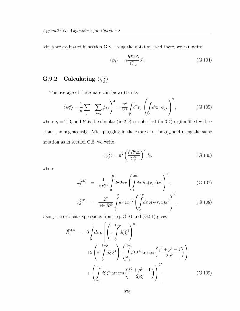
Appendix G: Appendices for Chapter 8
which we evaluated in section G.8. Using the notation used there, we can write
〈ψj〉 = n~R3∆
C312
J1. (G.104)
G.9.2 Calculating⟨ψ2j
⟩
The average of the square can be written as
⟨ψ2j
⟩=
1
n
∑
j
(∑
k 6=j
φj,k
)2
=n2
V 3
∫
V
dηrj
∫
V
dηrk φj,k
2
, (G.105)
where η = 2, 3, and V is the circular (in 2D) or spherical (in 3D) region filled with n
atoms, homogeneously. After plugging in the expression for φj,k and using the same
notation as in section G.8, we write
⟨ψ2j
⟩= n2
(~R3∆
C312
)2
J3, (G.106)
where
J(2D)3 =
1
πR12
R∫
0
dr 2πr
2R∫
0
dxSR(r, x)x3
2
, (G.107)
J(3D)3 =
27
64πR15
R∫
0
dr 4πr2
2R∫
0
dxAR(r, x)x3
2
. (G.108)
Using the explicit expressions from Eq. G.90 and (G.91) gives
J(2D)3 = 8
1∫
0
dρ ρ
π
1−ρ∫
0
dξ ξ4
2
+2
π
1−ρ∫
0
dξ ξ4
1+ρ∫
1−ρ
dξ ξ4 arccos
(ξ2 + ρ2 − 1
2ρξ
)
+
1+ρ∫
1−ρ
dξ ξ4 arccos
(ξ2 + ρ2 − 1
2ρξ
)
2 (G.109)
276

Appendix G: Appendices for Chapter 8
J(3D)3 = 27π2
1∫
0
dρ ρ2
1−ρ∫
0
dξ ξ5
2
+2
1−ρ∫
0
dξ ξ5
1+ρ∫
1−ρ
dξ1
4
ξ4
ρ
[1− (ξ − ρ)2
]
+
1+ρ∫
1−ρ
dξ1
4
ξ4
ρ[1− (ξ − ρ)2]
2 (G.110)
We evaluate these numerically and find J(2D)3 = 17.81, and J
(3D)3 = 25.16.
G.9.3 Result for Var(ψj)
Now, the variance in question can be written as
Var(ψj) =⟨ψ2j
⟩− 〈ψj〉2 = n2
(~R3∆
C(3)12
)2 [J3 − J2
1
]. (G.111)
After plugging in R = a(n/π)1/2 (for 2D) and R = a(3n/(4π))1/3 (for 3D), we get
Var(ψj)(2D) = 0.08359n5
(~a3∆
C(3)12
)2
(G.112)
Var(ψj)(3D) = 0.1277n4
(~a3∆
C(3)12
)2
(G.113)
G.10 Calculating Var(∆j)
Here, we calculate the variance of ∆j = −∑k 6=jΩ2
4(∆j,k+∆)≈ −∑k 6=j
Ω2
4∆jkin case
of ∆ min ∆j,k, for an ensemble of n atoms, trapped in a lattice with periodicity a,
uniformly filling a circular 2D (spherical 3D) region of radius R. We assume a van
der Waals interaction, ∆j,k =C
(6)11
~|rj−rk|6between pairs of atoms at rj and rk.
277
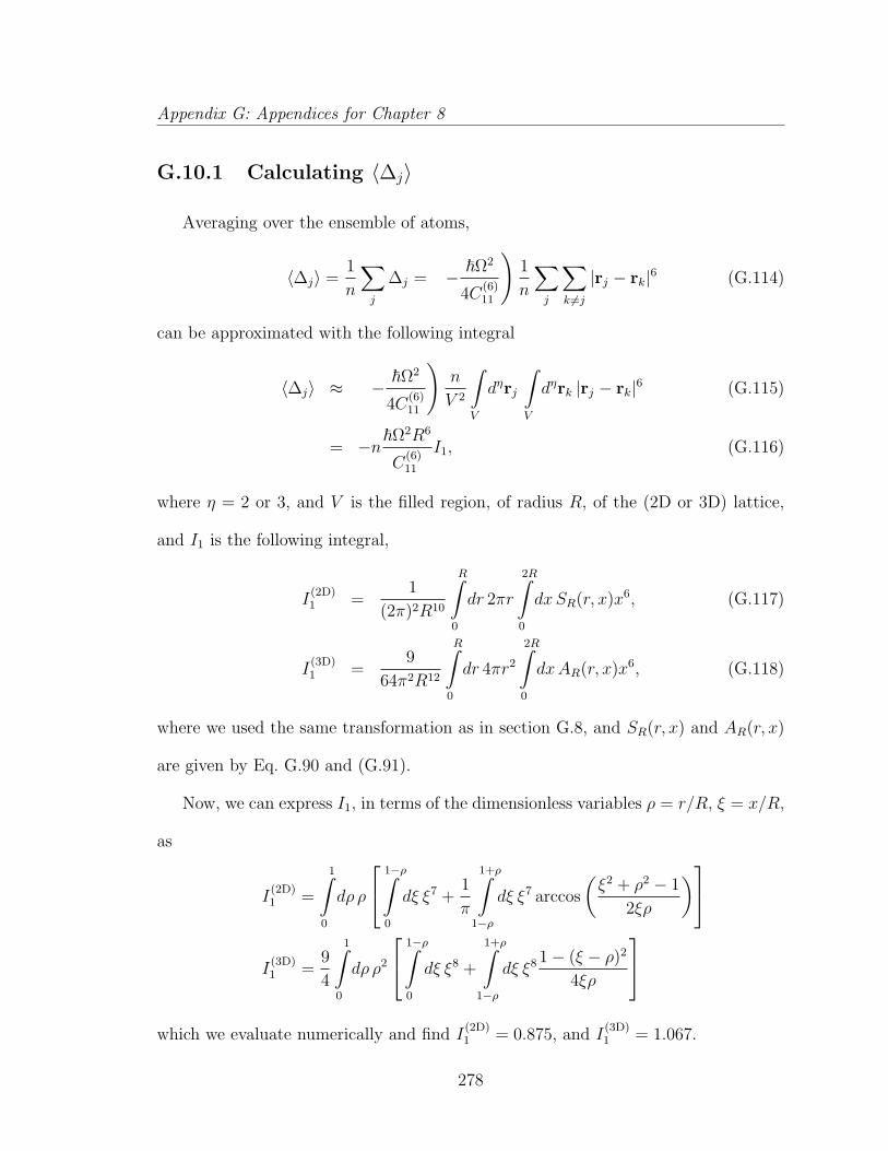
Appendix G: Appendices for Chapter 8
G.10.1 Calculating 〈∆j〉
Averaging over the ensemble of atoms,
〈∆j〉 =1
n
∑
j
∆j =
(− ~Ω2
4C(6)11
)1
n
∑
j
∑
k 6=j
|rj − rk|6 (G.114)
can be approximated with the following integral
〈∆j〉 ≈(− ~Ω2
4C(6)11
)n
V 2
∫
V
dηrj
∫
V
dηrk |rj − rk|6 (G.115)
= −n~Ω2R6
C(6)11
I1, (G.116)
where η = 2 or 3, and V is the filled region, of radius R, of the (2D or 3D) lattice,
and I1 is the following integral,
I(2D)1 =
1
(2π)2R10
R∫
0
dr 2πr
2R∫
0
dxSR(r, x)x6, (G.117)
I(3D)1 =
9
64π2R12
R∫
0
dr 4πr2
2R∫
0
dxAR(r, x)x6, (G.118)
where we used the same transformation as in section G.8, and SR(r, x) and AR(r, x)
are given by Eq. G.90 and (G.91).
Now, we can express I1, in terms of the dimensionless variables ρ = r/R, ξ = x/R,
as
I(2D)1 =
1∫
0
dρ ρ
1−ρ∫
0
dξ ξ7 +1
π
1+ρ∫
1−ρ
dξ ξ7 arccos
(ξ2 + ρ2 − 1
2ξρ
)
I(3D)1 =
9
4
1∫
0
dρ ρ2
1−ρ∫
0
dξ ξ8 +
1+ρ∫
1−ρ
dξ ξ8 1− (ξ − ρ)2
4ξρ
which we evaluate numerically and find I(2D)1 = 0.875, and I
(3D)1 = 1.067.
278
Appendix G: Appendices for Chapter 8
G.10.2 Calculating⟨∆2
j
⟩
The average of ∆2j can be written as
⟨∆2j
⟩=
1
n
∑
j
∆2j =
(~Ω2
4C(6)11
)21
n
∑
j
(∑
k 6=j
|rj − rk|6)2
. (G.119)
Similarly to the calculation of 〈∆j〉, we can approximate the sums with integrals and
write
⟨∆2j
⟩=
(n~Ω2R6
C(6)11
)2
I2, (G.120)
where I2 takes the following forms
I(2D)2 =
1
16π3R18
R∫
0
dr 2πr
2R∫
0
dxSR(r, x)x6
2
(G.121)
I(3D)2 =
27
256π3R21
R∫
0
dr 4πr2
2R∫
0
dxAR(r, x)x6
2
(G.122)
in the two cases.
After plugging in the explicit expressions of SR(r, x) and AR(r, x), we can express
I2 in terms of the dimensionless variables ρ = r/R, ξ = x/R, as
I(2D)2 =
1
2
1∫
0
dρ ρ
1−ρ∫
0
dξ ξ7
2
+2
π
1−ρ∫
0
dξ ξ7
1+ρ∫
1−ρ
dξ ξ7 arccos
(ξ2 + ρ2 − 1
2ξρ
)
+1
π2
1+ρ∫
1−ρ
dξ ξ7 arccos
(ξ2 + ρ2 − 1
2ξρ
)
2 , (G.123)
279

Appendix G: Appendices for Chapter 8
I(3D)2 =
27
16
1∫
0
dρ ρ2
1−ρ∫
0
dξ ξ8
2
+1
2
1−ρ∫
0
dξ ξ8
1+ρ∫
1−ρ
dξξ7
ρ[1− (ξ − ρ)2]
+1
16
1+ρ∫
1−ρ
dξξ7
ρ[1− (ξ − ρ)2]
2 (G.124)
which we evaluate numerically and find I(2D)2 = 1.146, and I
(3D)2 = 1.474
G.10.3 Result for Var(∆j)
Using the results above, we write the variance of ∆j as
Var(∆j) =⟨∆2j
⟩− 〈∆j〉2 = n2
(~Ω2R6
C(6)11
)[I2 − (I1)2
]. (G.125)
Instead of R, we can also write it, in terms of the lattice constant a, and the total
number of atoms n, as
Var(∆j)(2D) =
0.380
π6n8
(~Ω2a6
C(6)11
)2
, (G.126)
Var(∆j)(3D) =
81
128
0.336
π4n6
(~Ω2a6
C(6)11
)2
, (G.127)
where we used that R2π = na2 (in 2D) and 4πR3/3 = na3 (in 3D).
280
Bibliography
[1] Alex Abramovici, William E. Althouse, Ronald W. P. Drever, Yekta Gursel,Seiji Kawamura, Frederick J. Raab, David Shoemaker, Lisa Sievers, Robert E.Spero, Kip S. Thorne, Rochus E. Vogt, Rainer Weiss, Stanley E. Whitcomb,and Michael E. Zucker. Ligo: The laser interferometer gravitational-wave ob-servatory. Science, 256:325–333, 1992.
[2] U Akram, N Kiesel, M Aspelmeyer, and G J Milburn. Single-photon opto-mechanics in the strong coupling regime. New Journal of Physics, 12:083030,2010.
[3] Boris Albrecht, Pau Farrera, Xavier Fernandez-Gonzalvo, Matteo Cristiani, andHugues de Riedmatten. A waveguide frequency converter connecting rubidium-based quantum memories to the telecom c-band. Nature Communications,5:3376, 2013.
[4] D.W. Allan. Statistics of atomic frequency standards. Proceedings of the IEEE,54:221–230, 1966.
[5] Ulrik L. Andersen and Timothy C. Ralph. High-fidelity teleportation ofcontinuous-variable quantum states using delocalized single photons. Phys.Rev. Lett., 111:050504, 2013.
[6] A. Andre, A. S. Sørensen, and M. D. Lukin. Stability of atomic clocks basedon entangled atoms. Phys. Rev. Lett., 92:230801, 2004.
[7] Axel Andre. Nonclassical states of light and atomic ensembles: Generation andNew Applications. PhD thesis, Harvard University, 2005.
[8] Mauro Antezza, Caterina Braggio, Giovanni Carugno, Antonio Noto, RobertoPassante, Lucia Rizzuto, Giuseppe Ruoso, and Salvatore Spagnolo. Optome-chanical Rydberg-atom excitation via dynamic Casimir-Polder coupling. Phys.Rev. Lett., 113:023601, 2014.
[9] O. Arcizet, P.-F. Cohadon, T. Briant, M. Pinard, and A. Heidmann. Radiation-pressure cooling and optomechanical instability of a micromirror. Nature,444:71–74, 2006.
281
Bibliography
[10] Markus Aspelmeyer, Tobias J. Kippenberg, and Florian Marquardt. Cavityoptomechanics. Rev. Mod. Phys., 86:1391–1452, 2014.
[11] Markus Aspelmeyer and Keith Schwab. Focus on mechanical systems at thequantum limit. New Journal of Physics, 10:095001, 2008.
[12] F Bariani, Y O Dudin, T. A B Kennedy, and A Kuzmich. Dephasing of multi-particle Rydberg excitations for fast entanglement generation. Phys. Rev. Lett.,108:030501, 2012.
[13] J.A. Barnes and D.W. Allan. A statistical model of flicker noise. Proceedingsof the IEEE, 54:176–178, 1966.
[14] S Basiri-Esfahani, U Akram, and G J Milburn. Phonon number measurementsusing single photon opto-mechanics. New Journal of Physics, 14:085017, 2012.
[15] Almut Beige, Daniel Braun, Ben Tregenna, and Peter L. Knight. Quantumcomputing using dissipation to remain in a decoherence-free subspace. Phys.Rev. Lett., 85:1762–1765, 2000.
[16] Jan Benhelm, Gerhard Kirchmair, Christian F. Roos, and Rainer Blatt. To-wards fault-tolerant quantum computing with trapped ions. Nature Physics,4:463–466, 2008.
[17] C. H. Bennett and G. Brassard. In Proceedings IEEE International Conferenceon Computers, Systems and Signal Processing. IEEE, 1984.
[18] Charles H. Bennett, Gilles Brassard, Sandu Popescu, Benjamin Schumacher,John A. Smolin, and William K. Wootters. Purification of noisy entanglementand faithful teleportation via noisy channels. Phys. Rev. Lett., 76:722–725,1996.
[19] Nadja K. Bernardes, Ludmi la Praxmeyer, and Peter van Loock. Rate analysisfor a hybrid quantum repeater. Phys. Rev. A, 83:012323, 2011.
[20] H. Bernien, B. Hensen, W. Pfaff, G. Koolstra, M. S. Blok, L. Robledo, T. H.Taminiau, M. Markham, D. J. Twitchen, L. Childress, and R. Hanson. Heraldedentanglement between solid-state qubits separated by three metres. Nature,497:86–90, 2012.
[21] D. W. Berry, B. L. Higgins, S. D. Bartlett, M. W. Mitchell, G. J. Pryde, andH. M. Wiseman. How to perform the most accurate possible phase measure-ments. Phys. Rev. A, 80:052114, 2009.
282

Bibliography
[22] I. I. Beterov, M. Saffman, E. A. Yakshina, V. P. Zhukov, D. B. Tretyakov, V. M.Entin, I. I. Ryabtsev, C. W. Mansell, C. MacCormick, S. Bergamini, and M. P.Fedoruk. Quantum gates in mesoscopic atomic ensembles based on adiabaticpassage and Rydberg blockade. Phys. Rev. A, 88:010303, 2013.
[23] B. J. Bloom, T. L. Nicholson, J. R. Williams, S. L. Campbell, M. Bishof,X. Zhang, W. Zhang, S. L. Bromley, and J. Ye. An optical lattice clock withaccuracy and stability at the 10−18 level. Nature, 506:71–75, 2014.
[24] J. J . Bollinger, Wayne M. Itano, D. J. Wineland, and D. J. Heinzen. Opti-mal frequency measurements with maximally correlated states. Phys. Rev. A,54:R4649–R4652, 1996.
[25] J Borregaard, P. Komar, E. M. Kessler, M. D. Lukin, and A. S. Sørensen. Long-distance entanglement distribution using individual atoms in optical cavities.Phys. Rev. A, 92:012307, 2015.
[26] J. Borregaard, P. Komar, E. M. Kessler, A. S. Sørensen, and M. D. Lukin. Her-alded quantum gates with integrated error detection in optical cavities. Phys.Rev. Lett., 114:110502, 2015.
[27] J. Borregaard and A. S. Sørensen. Efficient atomic clocks operated with severalatomic ensembles. Phys. Rev. Lett., 111:090802, 2013.
[28] J. Borregaard and A. S. Sørensen. Near-heisenberg-limited atomic clocks in thepresence of decoherence. Phys. Rev. Lett., 111:090801, 2013.
[29] J. Borregaard, M. Zugenmaier, J. M. Petersen, H. Shen, G. Vasilakis, K. Jensen,E. S. Polzik, and A. S. Sørensen. Room temperature quantum memory andscalable single photon source based on motional averaging. arXiv:, 1501.03916,2015.
[30] Samuel L. Braunstein. Quantum limits on precision measurements of phase.Phys. Rev. Lett., 69:3598–3601, 1992.
[31] R. J. Brecha, P. R. Rice, and M. Xiao. n two-level atoms in a driven opticalcavity: Quantum dynamics of forward photon scattering for weak incident fields.Phys. Rev. A, 59:2392–2417, 1999.
[32] Ferdinand Brennecke, Stephan Ritter, Tobias Donner, and Tilman Esslinger.Cavity optomechanics with a bose-einstein condensate. Science, 322:235–238,2008.
[33] H.-J. Briegel, W. Dur, J. I. Cirac, and P. Zoller. Quantum repeaters: Therole of imperfect local operations in quantum communication. Phys. Rev. Lett.,81:5932–5935, 1998.
283
Bibliography
[34] A. Broadbent, J. Fitzsimons, and E. Kashefi. Universal blind quantum com-putation. In Foundations of Computer Science, 2009. FOCS ’09. 50th AnnualIEEE Symposium on, pages 517–526, 2009.
[35] Daniel E. Browne, Martin B. Plenio, and Susana F. Huelga. Robust creationof entanglement between ions in spatially separate cavities. Phys. Rev. Lett.,91:067901, 2003.
[36] Dagmar Bruß. Optimal eavesdropping in quantum cryptography with six states.Phys. Rev. Lett., 81:3018–3021, 1998.
[37] Michael J. Burek, Yiwen Chu, Madelaine S. Z. Liddy, Parth Patel, JakeRochman, Srujan Meesala, Wooyoung Hong, Qimin Quan, Mikhail D. Lukin,and Marko Loncar. High quality-factor optical nanocavities in bulk single-crystal diamond. Nature Communications, 5:5718, 2014.
[38] V. Buzek, R. Derka, and S. Massar. Optimal quantum clocks. Phys. Rev. Lett.,82:2207–2210, 1999.
[39] H.J. Carmichael, R.J. Brecha, and P.R. Rice. Quantum interference and collapseof the wavefunction in cavity qed. Optics Communications, 82:73 – 79, 1991.
[40] Tal Carmon and Kerry J. Vahala. Modal spectroscopy of optoexcited vibrationsof a micron-scale on-chip resonator at greater than 1 ghz frequency. Phys. Rev.Lett., 98:123901, 2007.
[41] Carlton M. Caves. Quantum-mechanical radiation-pressure fluctuations in aninterferometer. Phys. Rev. Lett., 45:75–79, 1980.
[42] Jasper Chan, T. P. Mayer Alegre, Amir H. Safavi-Naeini, Jeff T. Hill, AlexKrause, Simon Groblacher, Markus Aspelmeyer, and Oskar Painter. Lasercooling of a nanomechanical oscillator into its quantum ground state. Nature,478:89–92, 2011.
[43] Jasper Chan, Amir H. Safavi-Naeini, Jeff T. Hill, Sen Meenehan, and OskarPainter. Optimized optomechanical crystal cavity with acoustic radiation shield.Appl. Phys. Lett., 101:081115, 2012.
[44] D E Chang, A H Safavi-Naeini, M Hafezi, and O Painter. Slowing and stoppinglight using an optomechanical crystal array. New Journal of Physics, 13:023003,2011.
[45] Darrick E. Chang, Anders S. Sørensen, Eugene A. Demler, and Mikhail D.Lukin. A single-photon transistor using nanoscale surface plasmons. NaturePhysics, 3:807–812, 2007.
284
Bibliography
[46] Yu-Ao Chen, Xiao-Hui Bao, Zhen-Sheng Yuan, Shuai Chen, Bo Zhao, and Jian-Wei Pan. Heralded Generation of an Atomic NOON State. Phys. Rev. Lett.,104:043601, 2010.
[47] H. K. Cheung and C. K. Law. Nonadiabatic optomechanical hamiltonian of amoving dielectric membrane in a cavity. Phys. Rev. A, 84:023812, 2011.
[48] L. Childress, J. M. Taylor, A. S. Sørensen, and M. D. Lukin. Fault-tolerantquantum communication based on solid-state photon emitters. Phys. Rev. Lett.,96:070504, 2006.
[49] Lilian Childress, Ronald Walsworth, and Mikhail Lukin. Atom-like crystal de-fects: From quantum computers to biological sensors. Physics Today, 67:38,2014.
[50] Andrew M. Childs. Secure assisted quantum computation. Quantum Info.Comput., 5:456–466, 2005.
[51] Cheng Chin, Rudolf Grimm, Paul Julienne, and Eite Tiesinga. Feshbach reso-nances in ultracold gases. Rev. Mod. Phys., 82:1225–1286, 2010.
[52] C. W. Chou, D. B. Hume, J. C. J. Koelemeij, D. J. Wineland, and T. Rosen-band. Frequency comparison of two high-accuracy al+ optical clocks. Phys.Rev. Lett., 104:070802, 2010.
[53] Chin-Wen Chou, Julien Laurat, Hui Deng, Kyung Soo Choi, Hugues de Ried-matten, Daniel Felinto, and H. Jeff Kimble. Functional quantum nodes forentanglement distribution over scalable quantum networks. Science, 316:1316–1320, 2007.
[54] J. I. Cirac, P. Zoller, H. J. Kimble, and H. Mabuchi. Quantum state transfer andentanglement distribution among distant nodes in a quantum network. Phys.Rev. Lett., 78:3221–3224, 1997.
[55] C. W S Conover. Effects of pulse shape on strongly driven two-level systems.Phys. Rev. A, 84:1–15, 2011.
[56] Thomas Corbitt, Christopher Wipf, Timothy Bodiya, David Ottaway, DanielSigg, Nicolas Smith, Stanley Whitcomb, and Nergis Mavalvala. Optical dilutionand feedback cooling of a gram-scale oscillator to 6.9 mk. Phys. Rev. Lett.,99:160801, 2007.
[57] Harald Cramer. Mathematical Methods of Statistics. Princeton University Press,Princeton, NJ, 1946.
285
Bibliography
[58] Marcelo Davanco, Jasper Chan, Amir H. Safavi-Naeini, Oskar Painter, andKartik Srinivasan. Slot-mode-coupled optomechanical crystals. Opt. Express,20:24394–24410, 2012.
[59] Mark de Burgh and Stephen D. Bartlett. Quantum methods for clock synchro-nization: Beating the standard quantum limit without entanglement. Phys.Rev. A, 72:042301, 2005.
[60] Andrei Derevianko and Hidetoshi Katori. Colloquium : Physics of optical latticeclocks. Rev. Mod. Phys., 83:331–347, 2011.
[61] David Deutsch, Artur Ekert, Richard Jozsa, Chiara Macchiavello, SanduPopescu, and Anna Sanpera. Quantum privacy amplification and the securityof quantum cryptography over noisy channels. Phys. Rev. Lett., 77:2818–2821,1996.
[62] S. A. Diddams, J. C. Bergquist, S. R. Jefferts, and C. W. Oates. Standards oftime and frequency at the outset of the 21st century. Science, 306:1318–1324,2004.
[63] L. Ding, C. Baker, P. Senellart, A. Lemaitre, S. Ducci, G. Leo, and I. Favero.Wavelength-sized gaas optomechanical resonators with gigahertz frequency.Appl. Phys. Lett., 98:113108, 2011.
[64] Khelifa Djerroud, Ouali Acef, Andre Clairon, Pierre Lemonde, Catherine N.Man, Etienne Samain, and Peter Wolf. Coherent optical link through the tur-bulent atmosphere. Opt. Lett., 35:1479–1481, 2010.
[65] J. M. Dobrindt and T. J. Kippenberg. Theoretical analysis of mechanical dis-placement measurement using a multiple cavity mode transducer. Phys. Rev.Lett., 104:033901, 2010.
[66] P. Domokos, J. M. Raimond, M. Brune, and S. Haroche. Simple cavity-qedtwo-bit universal quantum logic gate: The principle and expected performances.Phys. Rev. A, 52:3554–3559, 1995.
[67] S. Droste, F. Ozimek, Th. Udem, K. Predehl, T. W. Hansch, H. Schnatz,G. Grosche, and R. Holzwarth. Optical-frequency transfer over a single-span1840 km fiber link. Phys. Rev. Lett., 111:110801, 2013.
[68] L.-M. Duan and H. J. Kimble. Efficient engineering of multiatom entanglementthrough single-photon detections. Phys. Rev. Lett., 90:253601, 2003.
[69] L.-M. Duan and H. J. Kimble. Scalable photonic quantum computation throughcavity-assisted interactions. Phys. Rev. Lett., 92:127902, 2004.
286
Bibliography
[70] L.-M. Duan, M. D. Lukin, J. I. Cirac, and P. Zoller. Long-distance quantumcommunication with atomic ensembles and linear optics. Nature, 414:413–418,2001.
[71] L.-M. Duan, B. Wang, and H. J. Kimble. Robust quantum gates on neutralatoms with cavity-assisted photon scattering. Phys. Rev. A, 72:032333, 2005.
[72] Lu-Ming Duan, G. Giedke, J. I. Cirac, and P. Zoller. Entanglement purificationof gaussian continuous variable quantum states. Phys. Rev. Lett., 84:4002–4005,2000.
[73] Y O Dudin and A Kuzmich. Strongly interacting Rydberg excitations of a coldatomic gas. Science, 336:887–9, 2012.
[74] Y O Dudin, A G Radnaev, R Zhao, J Z Blumoff, T A B Kennedy, andA Kuzmich. Entanglement of light-shift compensated atomic spin waves withtelecom light. Phys. Rev. Lett., 105:260502, 2010.
[75] W Dur and H J Briegel. Entanglement purification and quantum error correc-tion. Reports on Progress in Physics, 70:1381, 2007.
[76] W. Dur, H.-J. Briegel, J. I. Cirac, and P. Zoller. Quantum repeaters based onentanglement purification. Phys. Rev. A, 59:169–181, 1999.
[77] M. Ebert, M. Kwon, T. G. Walker, and M. Saffman. Coherence and rydbergblockade of atomic ensemble qubits. Phys. Rev. Lett., 115:093601, 2015.
[78] J. N. Eckstein, A. I. Ferguson, and T. W. Hansch. High-resolution two-photonspectroscopy with picosecond light pulses. Phys. Rev. Lett., 40:847–850, 1978.
[79] Matt Eichenfield, Jasper Chan, Ryan M. Camacho, Kerry J. Vahala, and OskarPainter. Optomechanical crystals. Nature, 462:78–82, 2009.
[80] Artur K. Ekert. Quantum cryptography based on bell’s theorem. Phys. Rev.Lett., 67:661–663, 1991.
[81] Dirk Englund, David Fattal, Edo Waks, Glenn Solomon, Bingyang Zhang,Toshihiro Nakaoka, Yasuhiko Arakawa, Yoshihisa Yamamoto, and JelenaVuckovic. Controlling the spontaneous emission rate of single quantum dotsin a two-dimensional photonic crystal. Phys. Rev. Lett., 95:013904, 2005.
[82] B. M. Escher, R. L. de Matos Filho, and L. Davidovich. General framework forestimating the ultimate precision limit in noisy quantum-enhanced metrology.Nature Physics, 7:406–411, 2011.
287
Bibliography
[83] Da-Wei Fang, Wei-Jun Xie, Yi Zhang, Xiao Hu, and Yu-Yan Liu. Radiativelifetimes of rydberg state of ytterbium. Journal of Quantitative Spectroscopyand Radiative Transfer, 69:469473, 2001.
[84] Ivan Favero and Khaled Karrai. Optomechanics of deformable optical cavities.Nature Photonics, 3:201–205, 2009.
[85] Richard P. Feynman. Simulating physics with computers. International Journalof Theoretical Physics, 21:467–488, 1982.
[86] Victor Fiore, Yong Yang, Mark C. Kuzyk, Russell Barbour, Lin Tian, andHailin Wang. Storing optical information as a mechanical excitation in a silicaoptomechanical resonator. Phys. Rev. Lett., 107:133601, 2011.
[87] Ofer Firstenberg, Thibault Peyronel, Qi-Yu Liang, Alexey V Gorshkov,Mikhail D Lukin, and Vladan Vuletic. Attractive photons in a quantum non-linear medium. Nature, 502:71–5, 2013.
[88] J. S. Foresi, P. R. Villeneuve, J. Ferrera, E. R. Thoen, G. Steinmeyer, S. Fan,J. D. Joannopoulos, L. C. Kimerling, Henry I. Smith, and E. P. Ippen. Photonic-bandgap microcavities in optical waveguides. Nature, 390:143–145, 1997.
[89] C. Gardiner and P. Zoller. Quantum Noise. Springer, 2004.
[90] C. Genes, A. Mari, D. Vitali, and P. Tombesi. Chapter 2 quantum effects inoptomechanical systems. In Advances in Atomic Molecular and Optical Physics,volume 57, pages 33 – 86. Academic Press, 2009.
[91] G. Giedke, J. M. Taylor, D. D’Alessandro, M. D. Lukin, and A. Imamoglu.Quantum measurement of a mesoscopic spin ensemble. Phys. Rev. A, 74:032316,2006.
[92] S. Gigan, H. R. Bohm, M. Paternostro, F. Blaser, G. Langer, J. B. Hertzberg,K. C. Schwab, D. Buerle, M. Aspelmeyer, and A. Zeilinger. Self-cooling of amicromirror by radiation pressure. Nature, 444:67–70, 2006.
[93] V. Giovannetti, D. Vitali, P. Tombesi, and A. Ekert. Scalable quantum com-putation with cavity qed systems. Phys. Rev. A, 62:032306, 2000.
[94] Vittorio Giovannetti, Seth Lloyd, and Lorenzo Maccone. Quantum metrology.Phys. Rev. Lett., 96:010401, 2006.
[95] Vittorio Giovannetti, Seth Lloyd, and Lorenzo Maccone. Advances in quantummetrology. Nature Photonics, 5:222–229, 2011.
288

Bibliography
[96] Nicolas Gisin, Gregoire Ribordy, Wolfgang Tittel, and Hugo Zbinden. Quantumcryptography. Rev. Mod. Phys., 74:145–195, 2002.
[97] Michael H Goerz, Eli J Halperin, Jon M Aytac, Christiane P Koch, and K Bir-gitta Whaley. Robustness of high-fidelity Rydberg gates with single-site ad-dressability. Phys. Rev. A, 90:032329, 2014.
[98] M. Grassl, Th. Beth, and T. Pellizzari. Codes for the quantum erasure channel.Phys. Rev. A, 56:33–38, 1997.
[99] Simon Groblacher, Klemens Hammerer, Michael R. Vanner, and Markus As-pelmeyer. Observation of strong coupling between a micromechanical resonatorand an optical cavity field. Nature, 460:724–727, 2009.
[100] Ivan S. Grudinin, Hansuek Lee, O. Painter, and Kerry J. Vahala. Phonon laseraction in a tunable two-level system. Phys. Rev. Lett., 104:083901, 2010.
[101] Subhadeep Gupta, Kevin L. Moore, Kater W. Murch, and Dan M. Stamper-Kurn. Cavity nonlinear optics at low photon numbers from collective atomicmotion. Phys. Rev. Lett., 99:213601, 2007.
[102] Michael J. W. Hall, Dominic W. Berry, Marcin Zwierz, and Howard M. Wise-man. Universality of the Heisenberg limit for estimates of random phase shifts.Phys. Rev. A, 85:041802, 2012.
[103] Klemens Hammerer, Anders S. Sørensen, and Eugene S. Polzik. Quantuminterface between light and atomic ensembles. Rev. Mod. Phys., 82:1041–1093,2010.
[104] Yang Han, Bing He, Khabat Heshami, Cheng-Zu Li, and Christoph Simon.Quantum repeaters based on Rydberg-blockade-coupled atomic ensembles.Phys. Rev. A, 81:052311, 2010.
[105] B. L. Higgins, D. W. Berry, S. D. Bartlett, H. M. Wiseman, and G. J. Pryde.Entanglement-free heisenberg-limited phase estimation. Nature, 450:392–396,2007.
[106] Jeff T. Hill, Amir H. Safavi-Naeini, Jasper Chan, and Oskar Painter. Coherentoptical wavelength conversion via cavity optomechanics. Nature Communica-tions, 3:1196, 2012.
[107] N. Hinkley, J. A. Sherman, N. B. Phillips, M. Schioppo, N. D. Lemke, K. Beloy,M. Pizzocaro, C. W. Oates, and A. D. Ludlow. An atomic clock with 10−18instability. Science, 341:1215–1218, 2013.
289
Bibliography
[108] T Honjo, H Takesue, H Kamada, Y Nishida, O Tadanaga, M Asobe, and K In-oue. Long-distance distribution of time-bin entangled photon pairs over 100 kmusing frequency up-conversion detectors. Optics Express, 15:13957, 2007.
[109] D. Hucul, I. V. Inlek, G. Vittorini, C. Crocker, S. Debnath, S. M. Clark, andC. Monroe. Modular entanglement of atomic qubits using photons and phonons.Nature Physics, 11:37–42, 2015.
[110] S. F. Huelga, C. Macchiavello, T. Pellizzari, A. K. Ekert, M. B. Plenio, andJ. I. Cirac. Improvement of frequency standards with quantum entanglement.Phys. Rev. Lett., 79:3865–3868, 1997.
[111] E.T. Jaynes and F.W. Cummings. Comparison of quantum and semiclassicalradiation theories with application to the beam maser. Proceedings of the IEEE,51:89–109, 1963.
[112] Liang Jiang, Jacob M. Taylor, Navin Khaneja, and Mikhail D. Lukin. Optimalapproach to quantum communication using dynamic programming. Proceedingsof the National Academy of Sciences, 104:17291–17296, 2007.
[113] J.R. Johansson, P.D. Nation, and Franco Nori. Qutip 2: A python framework forthe dynamics of open quantum systems. Computer Physics Communications,184:1234 – 1240, 2013.
[114] David J. Jones, Scott A. Diddams, Jinendra K. Ranka, Andrew Stentz,Robert S. Windeler, John L. Hall, and Steven T. Cundiff. Carrier-envelopephase control of femtosecond mode-locked lasers and direct optical frequencysynthesis. Science, 288:635–639, 2000.
[115] M. J. Kastoryano, F. Reiter, and A. S. Sørensen. Dissipative preparation ofentanglement in optical cavities. Phys. Rev. Lett., 106:090502, 2011.
[116] E. M. Kessler, P. Komar, M. Bishof, L. Jiang, a. S. Sø rensen, J. Ye, and M. D.Lukin. Heisenberg-limited atom clocks based on entangled qubits. Phys. Rev.Lett., 112:190403, 2014.
[117] H. J. Kimble. The quantum internet. Nature, 453:1023–1030, 2008.
[118] T. J. Kippenberg and K. J. Vahala. Cavity optomechanics: Back-action at themesoscale. Science, 321:1172–1176, 2008.
[119] Dustin Kleckner and Dirk Bouwmeester. Sub-kelvin optical cooling of a mi-cromechanical resonator. Nature, 444:75–78, 2006.
[120] E. Knill, R. Laflamme, and G. J. Milburn. A scheme for efficient quantumcomputation with linear optics. Nature, 409:46–52, 2001.
290
Bibliography
[121] P. Komar, E. M. Kessler, M. Bishof, L. Jiang, a. S. Sørensen, J. Ye, and M. D.Lukin. A quantum network of clocks. Nature Physics, 10:582–587, 2014.
[122] Andreas Kronwald, Max Ludwig, and Florian Marquardt. Full photon statisticsof a light beam transmitted through an optomechanical system. Phys. Rev. A,87:013847, 2013.
[123] Axel Kuhn, Markus Hennrich, and Gerhard Rempe. Deterministic single-photon source for distributed quantum networking. Phys. Rev. Lett., 89:067901,2002.
[124] T. D. Ladd, F. Jelezko, R. Laflamme, Y. Nakamura, C. Monroe, and J. L.OBrien. Quantum computers. Nature, 464:45–53, 2010.
[125] D. Leibfried, M. D. Barrett, T. Schaetz, J. Britton, J. Chiaverini, W. M. Itano,J. D. Jost, C. Langer, and D. J. Wineland. Toward heisenberg-limited spec-troscopy with multiparticle entangled states. Science, 304:1476–1478, 2004.
[126] N. D. Lemke, A. D. Ludlow, Z. W. Barber, T. M. Fortier, S. A. Diddams,Y. Jiang, S. R. Jefferts, T. P. Heavner, T. E. Parker, and C. W. Oates. Spin-1/2 optical lattice clock. Phys. Rev. Lett., 103:063001, 2009.
[127] Ian D. Leroux, Monika H. Schleier-Smith, and Vladan Vuletic. Implementationof cavity squeezing of a collective atomic spin. Phys. Rev. Lett., 104:073602,2010.
[128] L. Li, Y. O. Dudin, and A. Kuzmich. Entanglement between light and an opticalatomic excitation. Nature, 498:466–469, 2013.
[129] Jie-Qiao Liao and C. K. Law. Correlated two-photon scattering in cavity op-tomechanics. Phys. Rev. A, 87:043809, 2013.
[130] Anne Louchet-Chauvet, Jurgen Appel, Jelmer J Renema, Daniel Oblak, NielsKjaergaard, and Eugene S Polzik. Entanglement-assisted atomic clock beyondthe projection noise limit. New Journal of Physics, 12:065032, 2010.
[131] Andrew D. Ludlow and Jun Ye. Progress on the optical lattice clock. ComptesRendus Physique, 16:499 – 505, 2015.
[132] Max Ludwig, Bjrn Kubala, and Florian Marquardt. The optomechanical insta-bility in the quantum regime. New Journal of Physics, 10:095013, 2008.
[133] Max Ludwig, Amir H. Safavi-Naeini, Oskar Painter, and Florian Marquardt.Enhanced quantum nonlinearities in a two-mode optomechanical system. Phys.Rev. Lett., 109:063601, 2012.
291
Bibliography
[134] M. D. Lukin. Colloquium : Trapping and manipulating photon states in atomicensembles. Rev. Mod. Phys., 75:457–472, 2003.
[135] M. D. Lukin, M. Fleischhauer, R. Cote, L M Duan, D Jaksch, J I Cirac, andP Zoller. Dipole blockade and quantum information processing in mesoscopicatomic ensembles. Phys. Rev. Lett., 87:037901, 2001.
[136] Xiao-Song Ma, Thomas Herbst, Thomas Scheidl, Daqing Wang, SebastianKropatschek, William Naylor, Bernhard Wittmann, Alexandra Mech, JohannesKofler, Elena Anisimova, Vadim Makarov, Thomas Jennewein, Rupert Ursin,and Anton Zeilinger. Quantum teleportation over 143 kilometres using activefeed-forward. Nature, 489:269–273, 2012.
[137] H. Mabuchi and A. C. Doherty. Cavity quantum electrodynamics: Coherencein context. Science, 298:1372–1377, 2002.
[138] J. Majer, J. M. Chow, J. M. Gambetta, Jens Koch, B. R. Johnson, J. A.Schreier, L. Frunzio, D. I. Schuster, A. A. Houck, A. Wallraff, A. Blais, M. H.Devoret, S. M. Girvin, and R. J. Schoelkopf. Coupling superconducting qubitsvia a cavity bus. Nature, 449:443–447, 2007.
[139] Yuriy Makhlin, Gerd Scohn, and Alexander Shnirman. Josephson-junctionqubits with controlled couplings. Nature, 398:305–307, 1999.
[140] Atul Mantri, Carlos A. Perez-Delgado, and Joseph F. Fitzsimons. Optimalblind quantum computation. Phys. Rev. Lett., 111:230502, 2013.
[141] Florian Marquardt, Joe P. Chen, A. A. Clerk, and S. M. Girvin. Quantumtheory of cavity-assisted sideband cooling of mechanical motion. Phys. Rev.Lett., 99:093902, 2007.
[142] Florian Marquardt and Steven M. Girvin. Trend: Optomechanics. Physics,2:40, 2009.
[143] William Marshall, Christoph Simon, Roger Penrose, and Dik Bouwmeester.Towards quantum superpositions of a mirror. Phys. Rev. Lett., 91:130401, 2003.
[144] P. Maunz, D. L. Moehring, S. Olmschenk, K. C. Younge, D. N. Matsukevich,and C. Monroe. Quantum interference of photon pairs from two remote trappedatomic ions. Nature Physics, 3:538–541, 2007.
[145] P. C. Maurer, G. Kucsko, C. Latta, L. Jiang, N. Y. Yao, S. D. Bennett,F. Pastawski, D. Hunger, N. Chisholm, M. Markham, D. J. Twitchen, J. I.Cirac, and M. D. Lukin. Room-temperature quantum bit memory exceedingone second. Science, 336:1283–1286, 2012.
292
Bibliography
[146] Robert McConnell, Hao Zhang, Senka Cuk, Jiazhong Hu, Monika H. Schleier-Smith, and Vladan Vuletic. Generating entangled spin states for quantummetrology by single-photon detection. Phys. Rev. A, 88:063802, 2013.
[147] D Meiser, Jun Ye, and M J Holland. Spin squeezing in optical lattice clocks vialattice-based qnd measurements. New Journal of Physics, 10:073014, 2008.
[148] Attila Mekis, J. C. Chen, I. Kurland, Shanhui Fan, Pierre R. Villeneuve, andJ. D. Joannopoulos. High transmission through sharp bends in photonic crystalwaveguides. Phys. Rev. Lett., 77:3787–3790, 1996.
[149] Constanze Hohberger Metzger and Khaled Karrai. Cavity cooling of a mi-crolever. Nature, 432:1002–1005, 2004.
[150] Pierre Meystre. A short walk through quantum optomechanics. Annalen derPhysik, 525:215–233, 2013.
[151] Haixing Miao, Stefan Danilishin, Thomas Corbitt, and Yanbei Chen. Standardquantum limit for probing mechanical energy quantization. Phys. Rev. Lett.,103:100402, 2009.
[152] M. W. Mitchell. Metrology with entangled states. In Proc. SPIE 5893, Quan-tum Communications and Quantum Imaging III, volume 5893, pages 589310–589310–10, 2005.
[153] Thomas Monz, Philipp Schindler, Julio T. Barreiro, Michael Chwalla, DanielNigg, William A. Coish, Maximilian Harlander, Wolfgang Hansel, Markus Hen-nrich, and Rainer Blatt. 14-qubit entanglement: Creation and coherence. Phys.Rev. Lett., 106:130506, 2011.
[154] M. Muller, I. Lesanovsky, H. Weimer, H. P. Buchler, and P. Zoller. MesoscopicRydberg Gate Based on Electromagnetically Induced Transparency. Phys. Rev.Lett., 102:170502, 2009.
[155] Sreraman Muralidharan, Linshu Li, Jungsang Kim, Norbert Lutkenhaus,Mikhail D. Lukin, and Liang Jiang. Efficient long distance quantum communi-cation. arXiv:, 1509.08435, 2015.
[156] T. L. Nicholson, M. J. Martin, J. R. Williams, B. J. Bloom, M. Bishof, M. D.Swallows, S. L. Campbell, and J. Ye. Comparison of two independent sr opticalclocks with 1×10⁻¹⁷ stability at 103 s. Phys. Rev. Lett., 109:230801, 2012.
[157] T.L. Nicholson, S.L. Campbell, R.B. Hutson, G.E. Marti, B.J. Bloom, R.L.McNally, W. Zhang, M.D. Barrett, M.S. Safronova, G.F. Strouse, W.L. Tew,and J. Ye. Systematic evaluation of an atomic clock at 2×10⁻¹⁸total uncertainty.Nature Communications, 6:6896, 2015.
293
Bibliography
[158] Naomi H. Nickerson, Joseph F. Fitzsimons, and Simon C. Benjamin. Freelyscalable quantum technologies using cells of 5-to-50 qubits with very lossy andnoisy photonic links. Phys. Rev. X, 4:041041, 2014.
[159] M. A. Nielsen and I. L. Chuang. Quantum Computation and Quantum Infor-mation. Cambridge University Press, Cambridge, England,, 2011.
[160] M. Notomi, E. Kuramochi, and H. Taniyama. Ultrahigh-q nanocavity with 1dphotonic gap. Opt. Express, 16:11095–11102, 2008.
[161] A. Nunnenkamp, K. Børkje, and S. M. Girvin. Single-photon optomechanics.Phys. Rev. Lett., 107:063602, 2011.
[162] A. D. O’Connell, M. Hofheinz, M. Ansmann, Radoslaw C. Bialczak, M. Lenan-der, Erik Lucero, M. Neeley, D. Sank, H. Wang, M. Weides, J. Wenner, John M.Martinis, and A. N. Cleland. Quantum ground state and single-phonon controlof a mechanical resonator. Nature, 464:697–703, 2010.
[163] S. Olmschenk, D. N. Matsukevich, P. Maunz, D. Hayes, L.-M. Duan, andC. Monroe. Quantum teleportation between distant matter qubits. Science,323:486–489, 2009.
[164] Jiannis Pachos and Herbert Walther. Quantum computation with trapped ionsin an optical cavity. Phys. Rev. Lett., 89:187903, 2002.
[165] Oskar Painter, Kartik Srinivasan, John D O’Brien, Axel Scherer, and P DanielDapkus. Tailoring of the resonant mode properties of optical nanocavities intwo-dimensional photonic crystal slab waveguides. Journal of Optics A, 3:S161,2001.
[166] Jian-Wei Pan, Christoph Simon, Caslav Brukner, and Anton Zeilinger. En-tanglement purification for quantum communication. Nature, 410:1067–1070,2001.
[167] M Peev, C Pacher, R Alleaume, C Barreiro, J Bouda, W Boxleitner, T De-buisschert, E Diamanti, M Dianati, J F Dynes, S Fasel, S Fossier, M Furst,J-D Gautier, O Gay, N Gisin, P Grangier, A Happe, Y Hasani, M Hentschel,H Hubel, G Humer, T Langer, M Legre, R Lieger, J Lodewyck, T Lorunser,N Lutkenhaus, A Marhold, T Matyus, O Maurhart, L Monat, S Nauerth, J-BPage, A Poppe, E Querasser, G Ribordy, S Robyr, L Salvail, A W Sharpe,A J Shields, D Stucki, M Suda, C Tamas, T Themel, R T Thew, Y Thoma,A Treiber, P Trinkler, R Tualle-Brouri, F Vannel, N Walenta, H Weier, H We-infurter, I Wimberger, Z L Yuan, H Zbinden, and A Zeilinger. The secoqc quan-tum key distribution network in vienna. New Journal of Physics, 11:075001,2009.
294
Bibliography
[168] T. Pellizzari, S. A. Gardiner, J. I. Cirac, and P. Zoller. Decoherence, continuousobservation, and quantum computing: A cavity qed model. Phys. Rev. Lett.,75:3788–3791, 1995.
[169] S Perseguers, G J Lapeyre Jr, D Cavalcanti, M Lewenstein, and A Acın. Distri-bution of entanglement in large-scale quantum networks. Reports on Progressin Physics, 76:096001, 2013.
[170] T. P. Purdy, D. W. C. Brooks, T. Botter, N. Brahms, Z.-Y. Ma, and D. M.Stamper-Kurn. Tunable cavity optomechanics with ultracold atoms. Phys. Rev.Lett., 105:133602, 2010.
[171] P. Rabl. Photon blockade effect in optomechanical systems. Phys. Rev. Lett.,107:063601, 2011.
[172] J. M. Raimond, M. Brune, and S. Haroche. Manipulating quantum entangle-ment with atoms and photons in a cavity. Rev. Mod. Phys., 73:565–582, 2001.
[173] T. C. Ralph, A. J. F. Hayes, and Alexei Gilchrist. Loss-tolerant optical qubits.Phys. Rev. Lett., 95:100501, 2005.
[174] Norman F. Ramsey. A molecular beam resonance method with separated os-cillating fields. Phys. Rev., 78:695–699, 1950.
[175] C A Regal and K W Lehnert. From cavity electromechanics to cavity optome-chanics. Journal of Physics: Conference Series, 264:012025, 2011.
[176] J. Reichert, M. Niering, R. Holzwarth, M. Weitz, Th. Udem, and T. W. Hansch.Phase coherent vacuum-ultraviolet to radio frequency comparison with a mode-locked laser. Phys. Rev. Lett., 84:3232–3235, 2000.
[177] Andreas Reiserer, Norbert Kalb, Gerhard Rempe, and Stephan Ritter. A quan-tum gate between a flying optical photon and a single trapped atom. Nature,508:237–240, 2014.
[178] Florentin Reiter and Anders S. Sørensen. Effective operator formalism for openquantum systems. Phys. Rev. A, 85:032111, 2012.
[179] P.R. Rice and H.J. Carmichael. Single-atom cavity-enhanced absorption. i.photon statistics in the bad-cavity limit. Quantum Electronics, IEEE Journalof, 24:1351–1366, 1988.
[180] D. Riste, M. Dukalski, C. A. Watson, G. de Lange, M. J. Tiggelman, Ya. M.Blanter, K. W. Lehnert, R. N. Schouten, and L. DiCarlo. Deterministic en-tanglement of superconducting qubits by parity measurement and feedback.Nature, 502:350–354, 2013.
295
Bibliography
[181] Stephan Ritter, Christian Nolleke, Carolin Hahn, Andreas Reiserer, AndreasNeuzner, Manuel Uphoff, Martin Mucke, Eden Figueroa, Joerg Bochmann, andGerhard Rempe. An elementary quantum network of single atoms in opticalcavities. Nature, 484:195–200, 2012.
[182] Jacob T. Robinson, Christina Manolatou, Long Chen, and Michal Lipson. Ul-trasmall mode volumes in dielectric optical microcavities. Phys. Rev. Lett.,95:143901, 2005.
[183] T. Rosenband and D. R. Leibrandt. Exponential scaling of clock stability withatom number. arXiv:, 1303.6357, 2013.
[184] Till Rosenband. Numerical test of few-qubit clock protocols. arXiv:, 1203.0288,2012.
[185] A. Rubenok, J. A. Slater, P. Chan, I. Lucio-Martinez, and W. Tittel. Real-World Two-Photon Interference and Proof-of-Principle Quantum Key Distri-bution Immune to Detector Attacks. Phys. Rev. Lett., 111:130501, 2013.
[186] J. Rutman. Characterization of phase and frequency instabilities in precisionfrequency sources: Fifteen years of progress. Proceedings of the IEEE, 66:1048–1075, 1978.
[187] A. H. Safavi-Naeini, T. P. Mayer Alegre, J. Chan, M. Eichenfield, M. Winger,Q. Lin, J. T. Hill, D. E. Chang, and O. Painter. Electromagnetically inducedtransparency and slow light with optomechanics. Nature, 472:69–73, 2011.
[188] Amir H Safavi-Naeini and Oskar Painter. Proposal for an optomechanical trav-eling wave phonon-photon translator. New Journal of Physics, 13:013017, 2011.
[189] M. Saffman and K. Mølmer. Efficient multiparticle entanglement via asymmet-ric rydberg blockade. Phys. Rev. Lett., 102:240502, 2009.
[190] M. Saffman, T. G. Walker, and K. Mølmer. Quantum information with Rydbergatoms. Rev. Mod. Phys., 82:2313–2363, 2010.
[191] Nicolas Sangouard, Romain Dubessy, and Christoph Simon. Quantum repeatersbased on single trapped ions. Phys. Rev. A, 79:042340, 2009.
[192] Nicolas Sangouard, Christoph Simon, Hugues de Riedmatten, and NicolasGisin. Quantum repeaters based on atomic ensembles and linear optics. Rev.Mod. Phys., 83:33–80, 2011.
[193] Nicolas Sangouard, Christoph Simon, Bo Zhao, Yu-Ao Chen, Hugues de Ried-matten, Jian-Wei Pan, and Nicolas Gisin. Robust and efficient quantum re-peaters with atomic ensembles and linear optics. Phys. Rev. A, 77:062301,2008.
296
Bibliography
[194] G. Santarelli, Claude Audoin, A. Makdissi, P. Laurent, G.J. Dick, and C. Cla-iron. Frequency stability degradation of an oscillator slaved to a periodicallyinterrogated atomic resonator. Ultrasonics, Ferroelectrics, and Frequency Con-trol, IEEE Transactions on, 45:887–894, 1998.
[195] Valerio Scarani, Helle Bechmann-Pasquinucci, Nicolas J. Cerf, Miloslav Dusek,Norbert Lutkenhaus, and Momtchil Peev. The security of practical quantumkey distribution. Rev. Mod. Phys., 81:1301–1350, 2009.
[196] S. Schiemann, A. Kuhn, S. Steuerwald, and K. Bergmann. Efficient coher-ent population transfer in no molecules using pulsed lasers. Phys. Rev. Lett.,71:3637–3640, 1993.
[197] S. Schiller, G.M. Tino, P. Gill, C. Salomon, U. Sterr, E. Peik, A. Nevsky,A. Gorlitz, D. Svehla, G. Ferrari, N. Poli, L. Lusanna, H. Klein, H. Margo-lis, P. Lemonde, P. Laurent, G. Santarelli, A. Clairon, W. Ertmer, E. Rasel,J. Muller, L. Iorio, C. Lmmerzahl, H. Dittus, E. Gill, M. Rothacher, F. Flech-ner, U. Schreiber, V. Flambaum, Wei-Tou Ni, Liang Liu, Xuzong Chen, Jing-biao Chen, Kelin Gao, L. Cacciapuoti, R. Holzwarth, M.P. He, and W. Schfer.Einstein gravity explorera medium-class fundamental physics mission. Experi-mental Astronomy, 23:573–610, 2009.
[198] A. Schliesser, R. Riviere, G. Anetsberger, O. Arcizet, and T. J. Kippenberg.Resolved-sideband cooling of a micromechanical oscillator. Nature Physics,4:415–419, 2008.
[199] Michael Schmidt, Max Ludwig, and Florian Marquardt. Optomechanical cir-cuits for nanomechanical continuous variable quantum state processing. NewJournal of Physics, 14:125005, 2012.
[200] R. J. Schoelkopf and S. M. Girvin. Wiring up quantum systems. Nature,451:664–669, 2008.
[201] A. Seidel, M.P. Hess, J. Kehrer, W. Schafer, M. Kufner, M. Siccardi, L. Cac-ciapuoti, I.A. Sanches, and S. Feltham. The aces microwave link: Instrumentdesign and test results. In 2007 IEEE International Frequency Control Sym-posium Joint with the 21st European Frequency and Time Forum, pages 1295–1298. IEEE, 2007.
[202] Jacob F. Sherson, Hanna Krauter, Rasmus K. Olsson, Brian Julsgaard, Kle-mens Hammerer, Ignacio Cirac, and Eugene S. Polzik. Quantum teleportationbetween light and matter. Nature, 443:557–560, 2006.
[203] Peter W. Shor. Polynomial-time algorithms for prime factorization and discretelogarithms on a quantum computer. SIAM Journal on Computing, 26:1484–1509, 1997.
297
Bibliography
[204] Bruce W. Shore and Peter L. Knight. The jaynes-cummings model. Journal ofModern Optics, 40:1195–1238, 1993.
[205] David Shwa, Raphael D. Cohen, Alex Retzker, and Nadav Katz. Heraldedgeneration of Bell states using atomic ensembles. Phys. Rev. A, 88:063844,2013.
[206] Anders Sørensen and Klaus Mølmer. Quantum computation with ions in ther-mal motion. Phys. Rev. Lett., 82:1971–1974, 1999.
[207] Anders Sørensen and Klaus Mølmer. Entanglement and quantum computationwith ions in thermal motion. Phys. Rev. A, 62:022311, 2000.
[208] Anders S. Sørensen and Klaus Mølmer. Measurement induced entanglementand quantum computation with atoms in optical cavities. Phys. Rev. Lett.,91:097905, 2003.
[209] Anders S. Sørensen and Klaus Mølmer. Probabilistic generation of entanglementin optical cavities. Phys. Rev. Lett., 90:127903, 2003.
[210] Dan M. Stamper-Kurn. Cavity optomechanics with cold atoms. arXiv:,1204.4351, 2012.
[211] K. Stannigel, P. Komar, S. J. M. Habraken, S. D. Bennett, M. D. Lukin,P. Zoller, and P. Rabl. Optomechanical quantum information processing withphotons and phonons. Phys. Rev. Lett., 109:013603, 2012.
[212] K. Stannigel, P. Rabl, A. S. Sørensen, P. Zoller, and M. D. Lukin. Optomechan-ical transducers for long-distance quantum communication. Phys. Rev. Lett.,105:220501, 2010.
[213] Y. Tanaka, T. Asano, and S. Noda. Design of photonic crystal nanocavity withq -factor of ∼109. Lightwave Technology, Journal of, 26:1532–1539, 2008.
[214] B. Tapley, J. Ries, S. Bettadpur, D. Chambers, M. Cheng, F. Condi, B. Gunter,Z. Kang, P. Nagel, R. Pastor, T. Pekker, S. Poole, and F. Wang. Ggm02 animproved earth gravity field model from grace. Journal of Geodesy, 79:467–478,2005.
[215] J. M. Taylor, A. S. Sørensen, C. M. Marcus, and E. S. Polzik. Laser coolingand optical detection of excitations in a lc electrical circuit. Phys. Rev. Lett.,107:273601, 2011.
[216] J. D. Teufel, T. Donner, Dale Li, J. W. Harlow, M. S. Allman, K. Cicak, A. J.Sirois, J. D. Whittaker, K. W. Lehnert, and R. W. Simmonds. Sideband coolingof micromechanical motion to the quantum ground state. Nature, 475:359–363,2011.
298
Bibliography
[217] J. D. Teufel, Dale Li, M. S. Allman, K. Cicak, A. J. Sirois, J. D. Whittaker,and R. W. Simmonds. Circuit cavity electromechanics in the strong-couplingregime. Nature, 471:204–208, 2011.
[218] J. D. Thompson, T. G. Tiecke, N. P. de Leon, J. Feist, A. V. Akimov, M. Gul-lans, A. S. Zibrov, V. Vuletic, and M. D. Lukin. Coupling a single trappedatom to a nanoscale optical cavity. Science, 340:1202–1205, 2013.
[219] J. D. Thompson, B. M. Zwickl, A. M. Jayich, Florian Marquardt, S. M. Girvin,and J. G. E. Harris. Strong dispersive coupling of a high-finesse cavity to amicromechanical membrane. Nature, 452:72–75, 2007.
[220] T. G. Tiecke, J. D. Thompson, N. P. de Leon, L. R. Liu, V. Vuletic, andM. D. Lukin. Nanophotonic quantum phase switch with a single atom. Nature,508:241–244, 2014.
[221] E. Togan, Y. Chu, A. S. Trifonov, L. Jiang, J. Maze, L. Childress, M. V. G.Dutt, A. S. Sørensen, P. R. Hemmer, A. S. Zibrov, and M. D. Lukin. Quantumentanglement between an optical photon and a solid-state spin qubit. Nature,466:730–734, 2010.
[222] Turker Topcu. in preparation.
[223] Turker Topcu and Andrei Derevianko. Intensity landscape and the possibilityof magic trapping of alkali-metal Rydberg atoms in infrared optical lattices.Phys. Rev. A, 88:043407, 2013.
[224] Turker Topcu and Andrei Derevianko. Divalent Rydberg atoms in optical lat-tices: Intensity landscape and magic trapping. Phys. Rev. A, 89:023411, 2014.
[225] Gotz S. Uhrig. Keeping a quantum bit alive by optimized π-pulse sequences.Phys. Rev. Lett., 98:100504, 2007.
[226] E. Urban, T. A. Johnson, T. Henage, L. Isenhower, D. D. Yavuz, T. G. Walker,and M. Saffman. Observation of rydberg blockade between two atoms. NaturePhysics, 5:110–114, 2009.
[227] S. J. van Enk, J. I. Cirac, and P. Zoller. Ideal quantum communication overnoisy channels: A quantum optical implementation. Phys. Rev. Lett., 78:4293–4296, 1997.
[228] S. J. van Enk, J. I. Cirac, and P. Zoller. Purifying two-bit quantum gates andjoint measurements in cavity qed. Phys. Rev. Lett., 79:5178–5181, 1997.
299
Bibliography
[229] Michael Varnava, Daniel E. Browne, and Terry Rudolph. Loss tolerance inone-way quantum computation via counterfactual error correction. Phys. Rev.Lett., 97:120501, 2006.
[230] E. Verhagen, S. Deleglise, S. Weis, A. Schliesser, and T. J. Kippenberg.Quantum-coherent coupling of a mechanical oscillator to an optical cavity mode.Nature, 482:63–67, 2012.
[231] Herbert Walther, Benjamin T H Varcoe, Berthold-Georg Englert, and ThomasBecker. Cavity quantum electrodynamics. Reports on Progress in Physics,69:1325, 2006.
[232] T. M. Weber, M. Honing, T. Niederprum, T. Manthey, O. Thomas, V. Guarrera,M. Fleischhauer, G. Barontini, and H. Ott. Mesoscopic Rydberg-blockadedensembles in the superatom regime and beyond. Nature Physics, 11:157–161,2015.
[233] Hendrik Weimer, Markus Muller, Igor Lesanovsky, Peter Zoller, and Hans PeterBuchler. A rydberg quantum simulator. Nature Physics, 6:382–388, 2010.
[234] Stefan Weis, Remi Riviere, Samuel Deleglise, Emanuel Gavartin, Olivier Ar-cizet, Albert Schliesser, and Tobias J. Kippenberg. Optomechanically inducedtransparency. Science, 330:1520–1523, 2010.
[235] D. J. Wilson, C. A. Regal, S. B. Papp, and H. J. Kimble. Cavity optomechanicswith stoichiometric sin films. Phys. Rev. Lett., 103:207204, 2009.
[236] I. Wilson-Rae, N. Nooshi, W. Zwerger, and T. J. Kippenberg. Theory of groundstate cooling of a mechanical oscillator using dynamical backaction. Phys. Rev.Lett., 99:093901, 2007.
[237] D. J. Wineland, W. M C. Monroe, Itano, D. Leibfried, B. E. King, andD. M. Meekhof. Experimental issues in coherent quantum-state manipulationof trapped atomic ions. J. Res. Natl. Inst. Stand. Technol., 103:259, 1998.
[238] P. Wolf, Ch.J. Borde, A. Clairon, L. Duchayne, A. Landragin, P. Lemonde,G. Santarelli, W. Ertmer, E. Rasel, F.S. Cataliotti, M. Inguscio, G.M. Tino,P. Gill, H. Klein, S. Reynaud, C. Salomon, E. Peik, O. Bertolami, P. Gil,J. Pramos, C. Jentsch, U. Johann, A. Rathke, P. Bouyer, L. Cacciapuoti,D. Izzo, P. De Natale, B. Christophe, P. Touboul, S.G. Turyshev, J. Ander-son, M.E. Tobar, F. Schmidt-Kaler, J. Vigue, A.A. Madej, L. Marmet, M.-C.Angonin, P. Delva, P. Tourrenc, G. Metris, H. Muller, R. Walsworth, Z.H.Lu, L.J. Wang, K. Bongs, A. Toncelli, M. Tonelli, H. Dittus, C. Lmmerzahl,G. Galzerano, P. Laporta, J. Laskar, A. Fienga, F. Roques, and K. Sengstock.
300
Bibliography
Quantum physics exploring gravity in the outer solar system: the sagas project.Experimental Astronomy, 23:651–687, 2009.
[239] Chi Xiong, Wolfram H P Pernice, Xiankai Sun, Carsten Schuck, King Y Fong,and Hong X Tang. Aluminum nitride as a new material for chip-scale optome-chanics and nonlinear optics. New Journal of Physics, 14:095014, 2012.
[240] Jun Ye, Jin-Long Peng, R. Jason Jones, Kevin W. Holman, John L. Hall,David J. Jones, Scott A. Diddams, John Kitching, Sebastien Bize, James C.Bergquist, Leo W. Hollberg, Lennart Robertsson, and Long-Sheng Ma. Deliv-ery of high-stability optical and microwave frequency standards over an opticalfiber network. J. Opt. Soc. Am. B, 20:1459–1467, 2003.
[241] Nanfang Yu and Federico Capasso. Flat optics with designer metasurfaces.Nature Materials, 13:139–150, 2014.
[242] Jing Zhang, Kunchi Peng, and Samuel L. Braunstein. Quantum-state transferfrom light to macroscopic oscillators. Phys. Rev. A, 68:013808, 2003.
[243] Mian Zhang, Gustavo S. Wiederhecker, Sasikanth Manipatruni, ArthurBarnard, Paul McEuen, and Michal Lipson. Synchronization of micromechani-cal oscillators using light. Phys. Rev. Lett., 109:233906, 2012.
[244] Bo Zhao, Markus Muller, Klemens Hammerer, and Peter Zoller. Efficient quan-tum repeater based on deterministic Rydberg gates. Phys. Rev. A, 81:052329,2010.
[245] Shi-Biao Zheng. Implementation of toffoli gates with a single asymmetric heisen-berg xy interaction. Phys. Rev. A, 87:042318, 2013.
301