arX

iv:q

uant

-ph/

9702

053v

1 2

7 Fe

b 19

97

Quantum dynamics of cold trappedions, with application to quantum

computation

by

Daniel F. V. James

Theoretical Division (T–4)

Mailstop B-268

Los Alamos National Laboratory

Los Alamos, NM 87545

U.S.A.

TEL: (505)-667-0956

FAX: (505)-665-3909

email: dfvj@t4.lanl.gov

to be submitted to Applied Physics B: Lasers and Optics

Abstract

The theory of interactions between lasers and cold trapped ions as it pertains to the

design of Cirac-Zoller quantum computers is discussed. The mean positions of the

trapped ions, the eigenvalues and eigenmodes of the ions’ oscillations, the magnitude

of the Rabi frequencies for both allowed and forbidden internal transitions of the ions

and the validity criterion for the required Hamiltonian are calculated. Energy level

data for a variety of ion species is also presented.

PACS numbers: 32.80.Qk, 42.50.Vk, 89.80.+h

1

1 Introduction

A quantum computer is a device in which data can be stored in a network of quan-

tum mechanical two-level systems, such as spin-1/2 particles or two level atoms. The

quantum mechanical nature of such systems allows the possibility of a powerful new

feature to be incorporated into data processing, namely the capability of performing

logical operations upon quantum mechanical superpositions of numbers. Thus in a

conventional digital computer each data register is, throughout any computation, al-

ways in a definite state “1” or “0”; however in a quantum computer, if such a device

can be realized, each data register (or “qubit”) will be in an undetermined quantum

superposition of two states |1〉 and |0〉. Calculations would then be performed by ex-

ternal interactions with the various two-level systems that constitute the device, in

such a way that conditional gate operations involving two or more different qubits

can be realized. The final result would be obtained by measurement of the quantum

mechanical probability amplitudes at the conclusion of the calculation. Much of the

recent interest in practical quantum computing has been stimulated by the discovery

of a quantum algorithm which allows the determination of the prime factors of large

composite numbers efficiently [1], and of coding schemes that, provided operations on

the qubits can be performed within a certain threshold degree of accuracy, will allow

arbitarily complicated quantum computations to be performed reliably regardless of

operational error [2].

So far, the most promising hardware proposed for implementation of such a de-

vice seems to be the cold-trapped ion system devised by Cirac and Zoller [3]. Their

design, which is shown schematically in figure 1, consists of a string of ions stored in a

linear radio-frequency trap and cooled sufficiently that their motion, which is coupled

together due to the Coulomb force between them, is quantum mechanical in nature.

Each qubit would be formed by two internal levels of each ion, a laser being used

to perform manipulations of the quantum mechanical probability amplitudes of the

states; conditional two-qubit logic gates being realized with aid of the excitation or

de-excitation of quanta of the ions’ collective motion. For a more detailed description

of the concept of cold-trapped ion quantum computation, the reader is referred to the

article by Steane [4].

There are two distinct possibilities for the choice of the internal levels of the ion:

firstly the two states could be the ground state, and a metastable excited state of

the ion (or more precisely, sublevels of these states); secondly the two states could be

two nearly degenerate sublevels of the ground state. In the first case a single laser

2

would suffice to perform the required operations; in the second, two lasers would be

required to perform Raman transitions between the states, via a third level. Both of

these schemes have advantages: the first, which I will refer to as the “single photon”

scheme, has the great advantage of conceptual and experimental simplicity; the second,

the “Raman scheme”, offers the advantages of a very low rate for spontaneous decay

between the two nearly degenerate states and resilience against fluctuations of the

phase of the laser. This later scheme was recently used by the group headed by Dr. D.

J. Wineland at the National Institute of Science and Technology at Boulder, Colorado

to realize a quantum logic gate using a single trapped Beryllium ion [5].

In this paper I will discuss the theory of laser interactions with cold trapped ions

as it pertains to the design of a Cirac-Zoller quantum computer. I will conscentrate

on the “single photon scheme” as originally proposed by those authors, although much

of the analysis is also relevant to the “Raman scheme”. Fuller accounts of aspects of

this are availible in the literature: see for example [6], [7], [4]; however the derivation

of several results are presented here for the first time. I will also present relevant data

gleaned from various sources on some species of ion suitable for use in a quantum

computation.

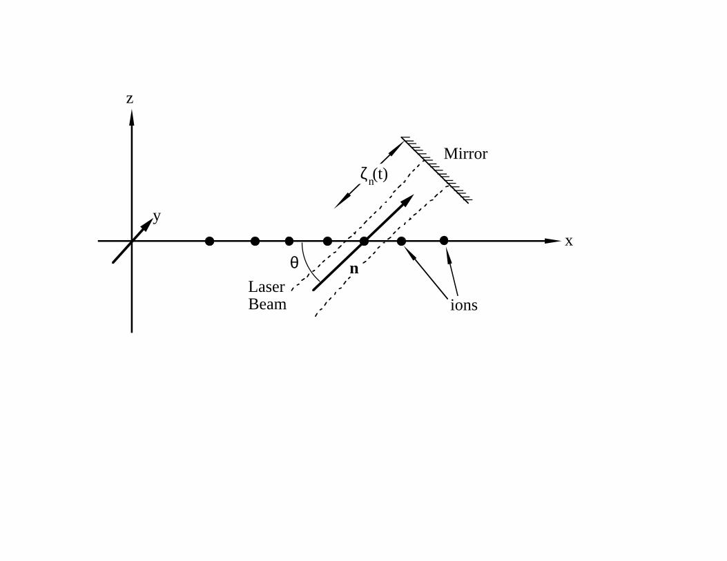
2 Equilibrium positions of ions in a linear trap

Let us consider a chain of N ions in a trap. The ions are assumed to be strongly

bound in the y and z directions but weakly bound in an harmonic potential in the x

direction. The position of the m − th ion, where the ions are numbered from left to

right, will be denoted xm(t). The motion of each ion will be influenced by an overall

harmonic potential due to the trap electrodes, and by the Coulomb force exerted by all

of the other ions. Hence the potential energy of the ion chain is given by the following

expression:

V =N∑

m=1

1

2Mν2xm(t)2 +

N∑

n,m=1m6=n

Z2e2

8πǫ0

1

|xn(t) − xm(t)| , (2.1)

where M is the mass of each ion, e is the electron charge, Z is the degree of ionization

of the ions, ǫ0 is the permitivity of free space and ν is the trap frequency, which

characterizes the strength of the trapping potential in the axial direction. Note that

this is an unconventional use of the symbol ν, which often denotes frequency rather

than angular frequency; following Cirac and Zoller, I will use ω to denote the angular

frequencies of the laser or the transitions between internal states of the ions, and ν to

3

denote angular frequencies associated with the motion of the ions.

Assume that the ions are sufficiently cold that the position of the m − th ion can

be approximated by the formula

xm(t) ≈ x(0)m + qm(t) (2.2)

where x(0)m is the equilibrium position of the ion, and qm(t) is a small displacement.

The equilibrium positions will be determined by the following equation:[

∂V

∂xm

]

xm=x(0)m

= 0 (2.3)

If we define the length scale ℓ by the formula

ℓ3 =Z2e2

4πǫ0Mν2, (2.4)

and the dimensionless equilibrium position um = x(0)m /ℓ, then (2.3) may be rewritten

as the following set of N coupled algebraic equations for the values of um:

um −m−1∑

n=1

1

(um − un)2+

N∑

n=m+1

1

(um − un)2= 0 (m = 1, 2, ..N) . (2.5)

For N = 2 and N = 3 these equations may be solved analytically:

N = 2 : u1 = −(1/2)2/3, u2 = (1/2)2/3 , (2.6)

N = 3 : u1 = −(5/4)1/3, u2 = 0, u3 = (5/4)1/3 . (2.7)

For larger values of N it is necessary to solve for the values of um numerically. The

numerical values of the solutions to these equations for 2 to 10 ions is given in table

1. Determining the solutions for larger numbers of ions is a straightforward but time

consuming task.

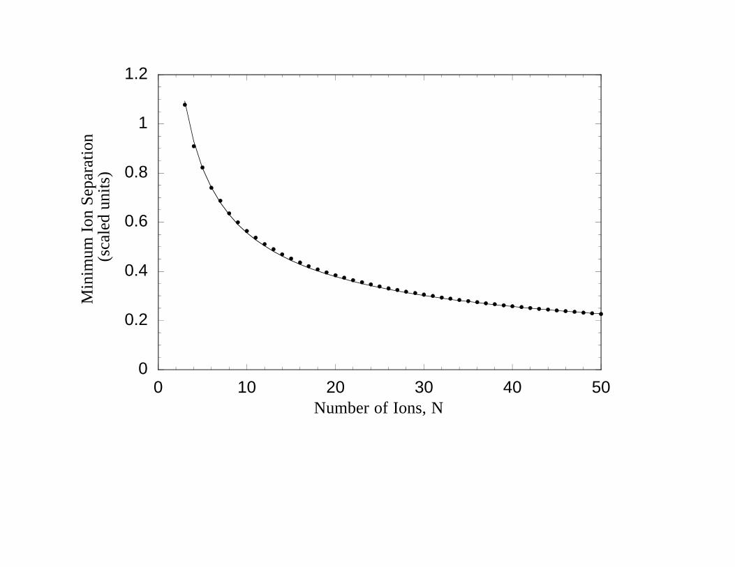
By inspection, the minimum value of the spacing between two adjacent ions occurs

at the center of the ion chain. Compiling the numerical data for the minimum value of

the separation for different numbers of trapped ions, we find that it obeys the following

relation:

umin(N) ≈ 2.018

N0.559. (2.8)

This relation is illustrated in figure 2. Thus the minimum inter-ion spacing for different

numbers of ions is given by the following formula:

xmin(N) =

(

Z2e2

4πǫ0Mν2

)1/32.018

N0.559. (2.9)

This relationship is important in determining the capabilities of cold trapped ion quan-

tum computers [8].

4

3 Quantum Fluctuations of the ions

This section discusses the equations of motion which describe the displacements of the

ions from their equilibrium positions. Because of the Coulomb interactions between

the ions, the displacements of different ions will be coupled together. The Lagrangian

describing the motion is then

L =M

2

N∑

m=1

(qm)2 − 1

2

N∑

n,m=1

qnqm

[

∂2V

∂xn∂xm

]

0

(3.1)

where the subscript 0 denotes that the double partial derivative is evaluated at qn =

qm = 0. The partial derivatives may be calculated explicitly to give the following

expression:

L =M

2

N∑

m=1

(qm)2 − ν2N∑

n,m=1

Anmqnqm

(3.2)

where

Anm =

1 + 2N∑

p=1p 6=m

1

|um − up|3if n = m,

−2

|um − un|3if n 6= m.

(3.3)

Since the matrix Anm is real, symmetric and non-negative definite, its eigenvalues

must be non-negative. The eigenvectors b(p)m (p = 1, 2, · · ·N) are therefore defined by

the following formula:

N∑

n=1

Anmb(p)n = µpb

(p)m (p = 1, . . . , N) , (3.4)

where µp ≥ 0. The eigenvectors are assumed to be numbered in order of increasing

eigenvalue and to be properly normalized so that

N∑

p=1

b(p)n b(p)

m = δnm (3.5)

N∑

n=1

b(p)n b(q)

n = δpq . (3.6)

The first eigenvector (i.e. the eigenvector with the smallest eigenvalue) can be

shown to be

b(1) =1√N

1, 1, . . . , 1 , µ1 = 1 . (3.7)

5

The next eigenvector can be shown to be

b(2) =1

(

N∑

m=1

u2m

)1/2u1, u2, . . . , uN , µ2 = 3 . (3.8)

Higher eigenvectors must, in general, be determined numerically. Equations (3.6) and

(3.7) imply thatN∑

m=1

b(p)m = 0 if p 6= 1. (3.9)

For N = 2 and N = 3, the eigenvectors and eigenvalues may be determined

algebraically:

N = 2 : b(1) =1√2(1, 1), µ1 = 1 ,

b(2) =1√2(−1, 1), µ2 = 3 ,

(3.10)

N = 3 : b(1) =1√3(1, 1, 1), µ1 = 1 ,

b(2) =1√2(−1, 0, 1), µ2 = 3 ,

b(3) =1√6(1,−2, 1), µ3 = 29/5 , (3.11)

For larger values of N , the eigenvalues and eigenvectors must be determined numeri-

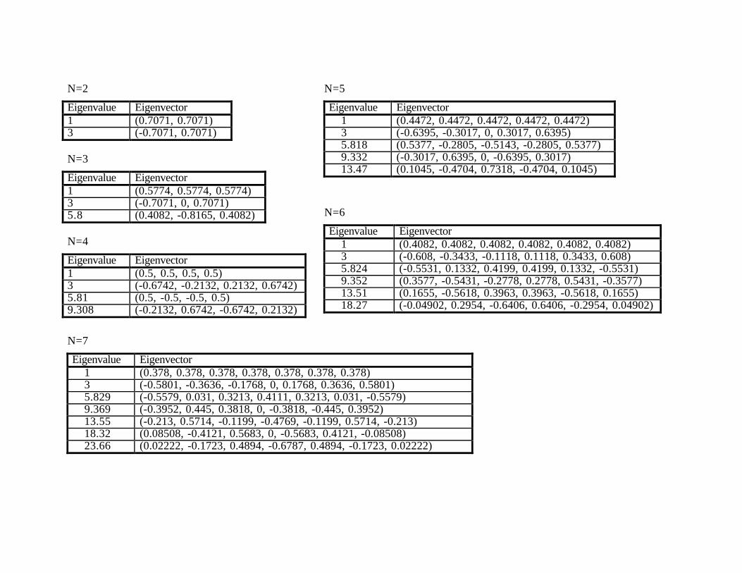
cally; their numerical values for 2 to 10 ions are given in table 2.

The normal modes of the ion motion are defined by the formula

Qp(t) =l∑

m=1

b(p)m qm(t) . (3.12)

The first mode Q1(t) corresponds to all of the ions oscillating back and forth as if they

were rigidly clamped together; this is referred to as the center of mass mode. The

second mode Q2(t) corresponds to each ion oscillating with an amplitude proportional

to its equilibrium distance form the trap center; This is called the breathing mode. The

Lagrangian for the ion oscillations (3.2) may be rewritten in terms of these normal

modes as follows:

L =M

2

N∑

p=1

[

Q2p − ν2

pQ2p

]

, (3.13)

6

where the angular frequency of the p − th mode is defined by

νp =√

µpν. (3.14)

This expression implies that the modes Qp are uncoupled. Thus the canonical mo-

mentum conjugate to Qp is Pp = MQp and one can immediately write the Hamiltonian

as

H =1

2M

N∑

p=1

P 2p +

M

2

N∑

p=1

ν2pQ

2p . (3.15)

The quantum motion of the ions can now be considered by introducing the operators 1

Qp → Qp = i

√

√

√

√

h

2Mνp

(

ap − a†p

)

, (3.16)

Pp → Pp =

√

hMνp

2

(

ap + a†p

)

. (3.17)

where Qp and Pp obey the canonical commutation relation[

Qp, Pq

]

= ihδpq and the

creation and annihilation operators a†p and ap obey the usual commutation relation

[

ap, a†q

]

= δpq.

Using this notation, the interaction picture operator for the displacement of the

m − th ion from its equilibrium position is given by the formula:

qm(t) =N∑

p=1

b(p)m Qp(t)

= i

√

h

2MνN

N∑

p=1

s(p)m

(

ape−iνpt − a†

peiνpt)

, (3.18)

where the coupling constant is defined by

s(p)m =

√Nb(p)

m

µ1/4p

. (3.19)

For the center of mass mode,

s(1)m = 1 ν1 = ν , (3.20)

and for the breathing mode

s(2)m =

√N

4√

3

1(

N∑

m=1

u2m

)1/2um ν2 =

√3ν . (3.21)

1There is some arbitarinees in the definition of the operators Pp and Qp, which is related to thearbitrariness of the phase of the Fock states. I have used the definitions given by Kittel (ref. [9], p.16),which differs from that given in other texts on quantum mechanics (see for example, ref. [10], p. 183or ref.[11] p. 36).

7

4 Laser-Ion interactions

I will now consider the interaction of a laser field with the trapped ions. The the-

ory must take into acount both the internal and vibrational degrees of freedom of the

ions. I will consider two types of transition between internal ionic levels: the familiar

electric-dipole allowed (E1) transitions and dipole forbidden electric quadrupole (E2)

transitions. Electric quadrupole transitions have been considered in detail by Freedhoff

[12],[13]. The reason for considering forbidden transitions is that they have very long

decay lifetimes; spontaneous emission will destroy the coherence of a quantum com-

puter, and therefore is a major limitation on the capabilities of such devices [14],[8].

Magnetic dipole (M1) transitions, which also have long lifetimes, tend only to occur

between sub-levels of a configuration, and will therefore require long wavelength lasers

in order to excite them. As it is necessary to resolve individual ions in the trap using

the laser, the use long wavelengths will seriously degrade performance. More highly

forbidden transitions are also a possibility for use in a quantum computer. In partic-

ular, there is a octupole allowed (E3) transition at 467nm with a theoretical lifetime

of 1.325 × 108 sec.[15], which has recently been observed at the National Physical

Laboratory at Teddington, England [16].

The interaction picture Hamitonians for electric dipole (E1) and electric quad-

rupole (E2) transitions of the m-th ion, located at xm are

H(E1)I = ie

∑

MN

ωMN |N〉〈M |〈N |ri|M〉Ai(xm, t)eiωMN t , (4.1)

H(E2)I =

ie

2

∑

MN

ωMN |N〉〈M |〈N |rirj |M〉∂iAj(xm, t)eiωMN t , (4.2)

where Aj(x, t) is the j − th component of the vector potential of the laser field, ∂i

denotes differentiation along the i− th direction and summation over repeated indices

(i, j = x, y, z) is implied; ri is the i − th component of the position operator for the

valence electron of the ion; |N〉 is the set of all eigenstates of the unperturbed ion

and the transition frequency is ωMN = ωM − ωN where the energy of the N − th state

is hωN .

For a laser beam in a standing wave configuration (see fig. 1), propagating along

a direction specified by the unit vector n, the vector potential and its derivative are

given by the formulas

Ai(xm, t) = −ǫiE

iωsin

[

kζm(t)]

eiωt + c.c., (4.3)

8

∂iAj(xm, t) = −niǫjE

ccos

[

kζm(t)]

eiωt + c.c. (4.4)

In (4.4), I have approximated the laser beam as a plane wave, ǫ being the polarization

vector, E is the amplitude of the electric field, ω is the laser frequency and k = ω/c is

the wavenumber. The operator ζm(t) is the distance between the m − th ion and the

plane mirror used to form the standing wave.

If we restrict our consideration to just two states, |1〉 and |2〉, and make the rotating

wave equation, the interaction Hamiltonians may be rewritten as follows:

H(E1)I = hΩ

(E1)0 sin

[

kζm(t)]

ei(t∆−φ)|1〉〈2| + h.a. , (4.5)

H(E2)I = ihΩ

(E2)0 cos

[

kζm(t)]

ei(t∆−φ)|1〉〈2| + h.a. , (4.6)

where the detuning is ∆ = ω − ω21 and the Rabi frequencies are given by

Ω(E1)0 =

∣

∣

∣

∣

eE

h〈1|ri|2〉ǫi

∣

∣

∣

∣

, (4.7)

Ω(E2)0 =

∣

∣

∣

∣

eEω21

2hc〈1|rirj|2〉ǫinj

∣

∣

∣

∣

. (4.8)

If the standing wave of the laser is so contrived that the equilibrium position of

the m − th ion is located at a node, i.e., the electric field strength is zero, then

ζm(t) = lλ + cosθqm(t) (4.9)

where l is some integer, λ is the wavelength, θ is the angle between the laser beam and

the trap axis and we have assumed that the fluctuations of the ions transverse to the

trap axis are negligible. In this case the two Hamiltonians become:

H(E1)I = hΩ

(E1)0 kcosθqm(t)ei(t∆−φ+lπ)|1〉〈2| + h.a. , (4.10)

H(E2)I = hΩ

(E2)0 ei[t∆−φ−(l+1/2)π]|1〉〈2| + h.a. , (4.11)

where we have neglected terms involving qm(t)2. It is convenient to write the dis-

placement of the ion in terms of the creation and annihilation operators of the phonon

modes, viz.:

kcosθqm(t) = iη√N

N∑

p=1

s(p)m

(

ape−iνpt − a†

peiνpt)

, (4.12)

where η =√

hk2cos2θ/ 2Mν is called the Lamb-Dicke parameter.

Similarly if the standing wave is arranged so that the ion is at an antinode, i.e.

ζm(t) =(2l − 1)λ

2+ cosθqm(t) (4.13)

9

then the Hamiltonians are:

H(E1)I = hΩ

(E1)0 ei(t∆−φ+lπ)|1〉〈2| + h.a. , (4.14)

H(E2)I = hΩ

(E2)0 kcosθqm(t)ei[t∆−φ−(l+1/2)π]|1〉〈2| + h.a. (4.15)

Thus we have two basic types of Hamiltonian:

HV = hΩ0ei(t∆−φv)|1〉〈2| + h.a. , (4.16)

HU = hΩ0kcosθqm(t)ei(t∆−φu)|1〉〈2| + h.a., (4.17)

where Ω0 stands for either Ω(E1)0 or Ω

(E2)0 .

By changing the node to an antinode, by moving the reflecting mirror for example,

we can switch from one type of Hamiltonian to the other. In the first case, the laser

beam will only interact with internal degrees of freedom of the ion, while in the second

case the collective motion of the ions will be affected as well.

5 Evaluation of the Rabi frequencies

We can relate the matrix elements appearing in the definitions of the Rabi frequencies

to the Einstein A coefficients for the transitions. In order to do this we will rewrite the

matrix elements in terms of the Racah tensors:

〈1|ri|2〉ǫi =1∑

q=−1

〈1|rC(1)q |2〉c(q)

i ǫi, (5.1)

〈1|rirj|2〉ǫinj =2∑

q=−2

〈1|r2C(2)q |2〉c(q)

ij ǫinj, (5.2)

where we have used the fact that ǫ ·n = 0. The vectors c(q) and the second rank tensors

c(q)ij may be calculated quite easily; explicit expressions are given in the appendix. If

we assume LS coupling, the states |1〉 and |2〉 are specified by the angular momentum

quantum numbers; thus we will use the notation |1〉 = |jmj〉 and |2〉 = |j′m′j〉 , where

j is the total angular momentum quantum number and mj the magnetic quantum

number of the lower state and j′ is the total angular momentum quantum number

and m′j the magnetic quantum number of the upper state. Using the Wigner-Eckart

theorem (ref. [17], section 11.4), the matrix elements may be rewritten as

〈1|ri|2〉ǫi = 〈1‖rC(1)‖2〉1∑

q=−1

(

j 1 j′

−mj q m′j

)

c(q)i ǫi, (5.3)

〈1|rirj |2〉ǫinj = 〈1‖r2C(2)‖2〉2∑

q=−2

(

j 2 j′

−m q m′

)

c(q)ij ǫinj , (5.4)

10

the terms containing six numbers in brackets being Wigner 3 − j symbols (ref. [17],

section 5.1), and 〈1‖rqC(q)‖2〉 being the reduced matrix element. The Einstein A

coefficients for the two levels are given by the expressions:

A(E1)12 =

4cαk312

3

1∑

q=−1

∣

∣

∣〈1|rC(1)q |2〉

∣

∣

∣

2(5.5)

A(E2)12 =

cαk512

15

2∑

q=−2

∣

∣

∣〈1|r2C(2)q |2〉

∣

∣

∣

2. (5.6)

Using the Wigner-Eckart theorem again, these expressions reduce to the following:

A(E1)12 =

4cαk312

3

∣

∣

∣〈1‖rC(1)‖2〉∣

∣

∣

21∑

q=−1

(

j 1 j′

−mj q m′j

)2

(5.7)

A(E2)12 =

cαk512

15

∣

∣

∣〈1‖r2C(2)‖2〉∣

∣

∣

22∑

q=−2

(

j 2 j′

−mj q m′j

)2

. (5.8)

These coefficients are the rates for spontaneous decay from the upper level |1〉 to

the lower level |2〉. A simpler expression for the total rate of spontaneous decay of |2〉to all of the sublevels of the lower state may be found by summing these rates over all

values of mj:

A(E1)12 ≡

j∑

m=−j

A(E1)12 =

4cαk312

3(2j′ + 1)

∣

∣

∣〈1‖rC(1)‖2〉∣

∣

∣

2(5.9)

A(E2)12 ≡

j∑

m=−j

A(E2)12 =

cαk512

15(2j′ + 1)

∣

∣

∣〈1‖r2C(2)‖2〉∣

∣

∣

2. (5.10)

These decay rates, which are the same for all of the sublevels of the upper level, are

the quantities usually quoted in data tables. Using (4.7-4.8), (5.3-5.4) and (5.9-5.10),

we then obtain the following formula for the Rabi frequencies:

Ω0 =e|E|h√

cα

√

A12

k312

σ, (5.11)

where

σ(E1) =

√

3(2j′ + 1)

4

∣

∣

∣

∣

∣

∣

1∑

q=−1

(

j 1 j′

−mj q m′j

)

c(q)i ǫi

∣

∣

∣

∣

∣

∣

, (5.12)

σ(E2) =

√

15(2j′ + 1)

4

∣

∣

∣

∣

∣

∣

2∑

q=−2

(

j 2 j′

−mj q m′j

)

c(q)ij ǫinj

∣

∣

∣

∣

∣

∣

. (5.13)

11

The values of these quantities will be dependent on the choice of states of ions

used for the upper and lower levels, and upon the polarization and direction of the laser

beam. As a specific example, we will assume that the ions are in a weak magnetic field,

which serves to define the z-direction of quantization. Furthermore, we will assume that

the lower level |1〉 is the mj = −1/2 sublevel of a 2S1/2 ground state, the nucleus having

spin zero. The upper level for the dipole transition is a sublevel of a 2P1/2 state, while

for the quadrupole transition it is a sublevel of a 2D3/2 state.

Ω(E1)0 =

e|E|h

√

√

√

√

A(E1)12

4cαk312

, (5.14)

Ω(E2)0 =

e|E|h

√

√

√

√

A(E2)12

2cαk312

. (5.15)

6 Validity of Cirac and Zoller’s Hamiltonian

Equations (4.12) and (4.17) give the following expression for the Hamiltonian for the

case when the laser standing wave is so configured that it can excite the vibration

modes of the ions:

HU =iηhΩ0√

N

N∑

p=1

s(p)m

(

ape−iνpt − a†

peiνpt)

ei(t∆−φu)|1〉〈2| + h.a., (6.1)

In their paper [3], Cirac and Zoller assumed that the laser can interact with only

the center of mass mode of the ions’ fluctuations. This interaction forms a vitally

important element of their proposed method for implementing a quantum controlled

not logic gate. Thus they used a Hamiltonian of the following form [c.f. ref.[3], eq. (1)]

H(CZ)U =

iηhΩ0√N

(

ape−iν1t − a†

peiν1t)

ei(t∆−φu)|1〉〈2| + h.a. (6.2)

This is an approximate form of (6.1), in which all of the other “extraneous” phonon

modes have been neglected. We will now investigate under what circumstances these

modes may be ignored.

We will assume that the wavefunction for a single ion interacting with the laser

beam may be written as follows:

|Ψ(t)〉 = α0(t)|1〉|vac〉 + b0(t)|2〉|vac〉 +N∑

p=1

αp(t)|1〉|1p〉 +N∑

p=1

bp(t)|2〉|1p〉, (6.3)

12

where |1〉 and |2〉 are the energy eigenstates of the m − th ion’s internal degrees of

freedom, |1p〉 is the state of the ions’ collective vibration in which the p − th mode

has been excited by one quantum, and |vac〉 is the vibrational ground state. To avoid

ambiguity, the ket for the ion’s internal state appears first, the ket for the vibrational

state second.

The equation of motion for this wavefunction is

ih∂

∂t|Ψ(t)〉 = HU |Ψ(t)〉. (6.4)

Using (6.1), and assuming that one cannot excite states with two phonons, one obtains

the following equations:

α0 =Ω0η√

N

N∑

p=1

s(p)m βp(t) (6.5)

β0 =Ω0η√

N

N∑

p=1

s(p)m αp(t) (6.6)

αp = −i(νp − ν1)αp −Ω0η√

Ns(p)

m β0(t) (6.7)

βp = −i(νp + ν1)βp −Ω0η√

Ns(p)

m α0(t) (6.8)

We have assumed that ∆ = −ν1, so that the laser is tuned to the specific sideband

resonance required to perform Cirac and Zoller’s universal gate operation (ref.[3], eq.

3), namely the two level transition |1〉n|11〉 ↔ |2〉n|vac〉.Since |α0(t)|, |β0(t)| ≤ 1, we can consider the following upper limits on the ampli-

tudes of the states which include excitation of “extraneous” phonon modes (i.e. phonon

modes other than the center of mass mode):

|αp(t)| ≤ |Ap(t)|, |βp(t)| ≤ |Bp(t)| (6.9)

where

A0 + i(νp − ν1)Ap = −Ω0η√N

s(p)m (6.10)

B0 + i(νp + ν1)Bp = −Ω0η√N

s(p)m . (6.11)

Solving these equations one finds that

|Ap(t)| ≤ 2Ω0η√N(νp − ν1)

|s(p)m | (6.12)

|Bp(t)| ≤ 2Ω0η√N(νp + ν1)

|s(p)m |, (6.13)

13

Thus the total probability that “extraneous” modes are excited has the following upper

limit:

Pext =N∑

p=2

|αp(t)|2 + |βp(t)|2 ≤ 2

(

2Ω0η√Nν

)2

N∑

p=2

µp + 1

(µp − 1)2(s(p)

m )2

, (6.14)

where we have used the definition of the mode frequencies (3.14) and the fact that the

eigenvalue for the center of mass mode is µ1 = 1. This quantity will be different for

each ion in the string; taking its average value, we find

Pext ≡ 1

N

N∑

m=1

Pext

≤ 2

(

2Ω0η√Nν

)2

Σ(N), (6.15)

where we have used the definition of the coupling constants, (3.19) and the orthonor-

mality of the eigenvectors (3.6). The function Σ(N) is defined by the formula

Σ(N) =N∑

p=2

µp + 1

(µp − 1)2√µp. (6.16)

This must be evaluated numerically by solving for the eigenvalues of the trap normal

modes for different numbers of trapped ions N . The results are shown in fig. (3). The

function varies slowly with the value of N , and , for N ≥ 10, we can, to a good approx-

imation, replace it by a constant Σ(N) ≈ 0.82. Thus we obtain the following upper

limit on the total probability of the “extraneous” phonon modes becoming excited:

Pext ≤(

2.6 Ω0η√Nν

)2

. (6.17)

Thus we obtain the following sufficiency condition for the validity of Cirac and Zoller’s

Hamiltonian (6.2):(

2.6 Ω0η√Nν

)2

≪ 1. (6.18)

7 Conclusion

In this preceeding sections we have reviewed the theoretical basis for cold trapped ion

quantum computation. How these various laser-ion interaction effects may be combined

to perform fundamental quantum logic gates is descibed in the seminal work of Cirac

14

and Zoller [3]. Using the formulae given here one can determine, for example, the laser

field strength required or the separation between ions in the trap. Such things are of

great importance in the engineering of practical devices.

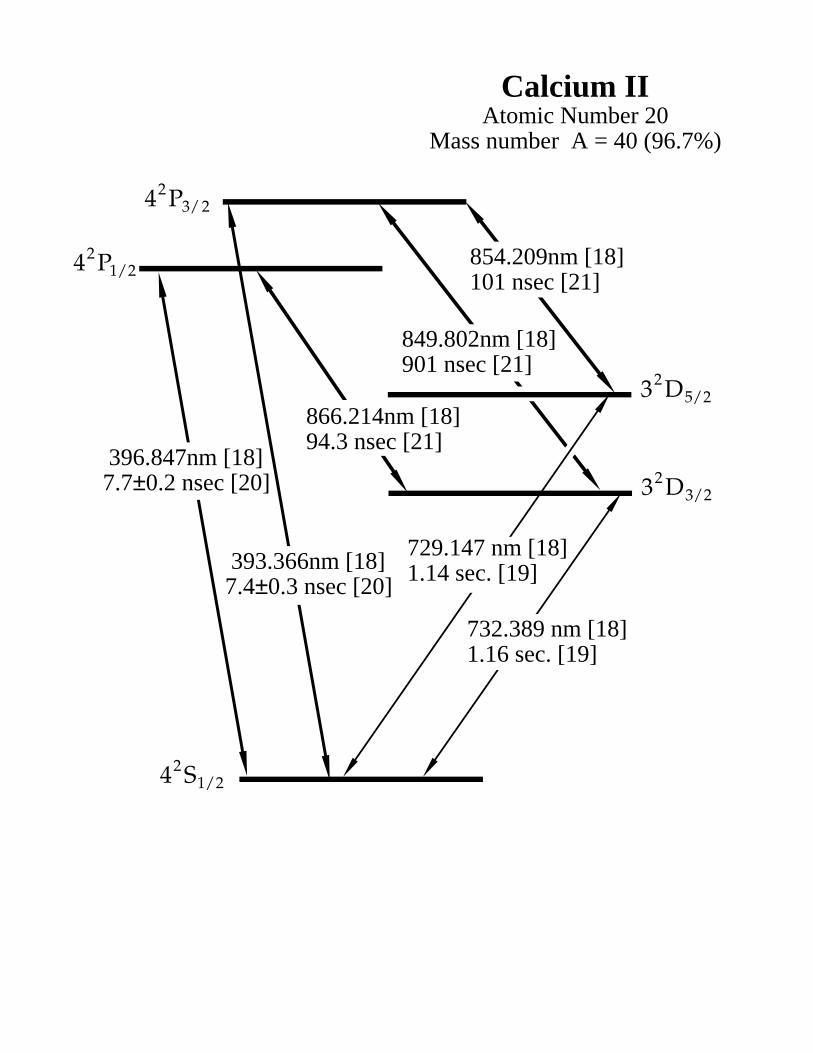
Finally there is the question of what type of ion to use. Figure 4 show the energy

levels of four suitable species of ion. These have been chosen based two criteria: that

the lowest excited state has a forbidden transition to the ground state, and their

popularity amoungst published ion trapping experiments. It is not intended that this

is an exhaustive list of suitable ions, but rather it is to show the properties of typical

ions.

Acknowledgments

The author would like to thank Barry Sanders (Macquarie University, Australia) and

Ignacio Cirac (University of Innsbruch, Austria) for useful discussions and Albert

Petschek (Los Alamos National Laboratory, USA) for reading an earlier version of

the manuscript. This work was funded by the National Security Agency.

Appendix

The vectors c(q)i are usual normalized spherical basis vectors:

c(1) = − 1√2(1,−i, 0), (A.1)

c(0) = (0, 0, 1), (A.2)

c(−1) =1√2(1, i, 0). (A.3)

(A.4)

Note that

c(q) = (−1)qc(−q)∗ (A.5)

c(q) ·

c(q′)∗

= δq,q′. (A.6)

The second rank tenors c(q)ij are given by the formula

c(q)ij =

√

10

3(−1)q

1∑

m1,m2=−1

(

1 1 2m1 m2 −q

)

c(m1)i c

(m2)j . (A.7)

15

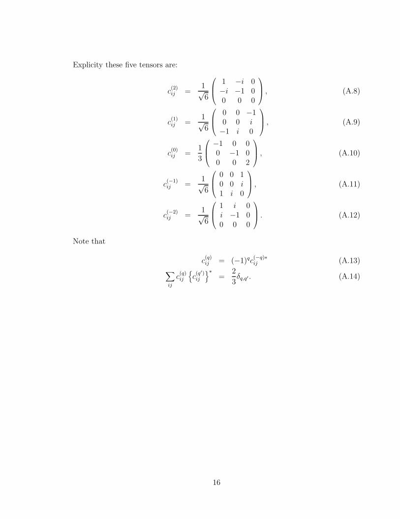
Explicity these five tensors are:

c(2)ij =

1√6

1 −i 0−i −1 00 0 0

, (A.8)

c(1)ij =

1√6

0 0 −10 0 i−1 i 0

, (A.9)

c(0)ij =

1

3

−1 0 00 −1 00 0 2

, (A.10)

c(−1)ij =

1√6

0 0 10 0 i1 i 0

, (A.11)

c(−2)ij =

1√6

1 i 0i −1 00 0 0

. (A.12)

Note that

c(q)ij = (−1)qc

(−q)∗ij (A.13)

∑

ij

c(q)ij

c(q′)ij

∗=

2

3δq,q′. (A.14)

16

References

[1] P. W. Shor: Proceedings of the 35th Annual Symposium on the Foundations of

Computer Science, S. Goldwasser ed., (IEEE Computer Society Press, Los Alami-

tos CA, 1994).

[2] E. Knill, R. Laflamme and W. Zurek:“Accuracy threshold for quantum comp-

utation”, Los Alamos Quantum Physics electronic reprint achive paper number

9610011 (15 Oct 1996), accessible via the world wide web at http://xxx.lanl. gov-

/list/quant-ph/9610; to be submitted to Science, 1997.

[3] J. I. Cirac and P. Zoller: Phys. Rev. Lett. 74, 4094 (1995).

[4] A. M. Steane: “The Ion Trap Quantum Information Processor”, Los Alamos

Quantum Physics electronic reprint achive paper number 9608011 (9 Aug 96),

accessible via the world wide web at http://xxx.lanl.gov/list/quant-ph/9608; Ap-

plied Physics B, in the press, 1997.

[5] C. Monroe, D. M. Meekhof, B. E. King, W. M. Itano and D. J. Wineland: Phys.

Rev. Lett. 75, 4714 (1995).

[6] D. J. Wineland and W. M. Itano: Phys. Rev. A20, 1521 (1979).

[7] J. I. Cirac, R, Blatt, P. Zoller and W. D. Phillips: Phys. Rev. A46, 2668 (1992).

[8] R. J. Hughes, D. F. V. James, E. H. Knill, R. Laflamme and A. G. Petschek:

Phys. Rev. Lett.77, 3240 (1996).

[9] C. Kittel: Quantum Theory of Solids (2nd edition, Wiley, New York,1987).

[10] L. I. Schiff: Quantum Mechanics (3rd Edition, McGraw Hill, Singapore, 1968).

[11] P. W. Milonni: The Quantum Vacuum (Academic Press, Boston,1994).

[12] H. S. Freedhoff: J. Chem. Phys. 54, 1618 (1971).

[13] H. S. Freedhoff: J. Phys. B 22, 435 (1989).

[14] M. B. Plenio and P. L. Knight: Phys. Rev. A 53, 2986 (1995).

[15] B. C. Fawcett and M. Wilson: Atomic Data and Nuclear Data Tables 47, 241

(1991).

17

[16] M. Roberts, P. Taylor, G. P. Barwood, P. Gill, H. A. Klein, and W. R. C. Rowley,

“Observation of an electric octupole transition in a single ion”, Phys. Rev. Lett.,

in the press, 1997.

[17] R. D. Cowan: The theory of atomic structure and spectra (University of California

Press, Berkeley, CA, 1981).

[18] S. Bashkin and J. O. Stoner, Atomic Energy-Level and Grotrian Diagrams Vol II

(North Holland, Amsterdam, 1978), pp 360-361.

[19] N. Vaeck, M. Godefroid and C. Froese Fischer: Phys. Rev. A 46, 3704 (1992).

[20] Accurate values for the total lifetimes of the P states of Ca+ are given in R. N.

Gosselin, E. H. Pinnington and W. Ansbacher: Phys. Rev. A 38, 4887 (1988);

the lifetimes of the S-P transitions can be calculated using this data and the data

from the NBS tables [21].

[21] W. L. Wiese, M. W. Smith and B. M. Miles : Atomic Transition Probabilities, Vol

II, (U. S. Government Printing Office, Washington, 1969), p.251.

[22] C. E. Moore: Atomic Energy Levels vol II, (National Bureau of Standards, Wash-

ington, 1952)

[23] G. P. Barwood, C. S. Edwards, P. Gill, G. Huang, H. A. Klein, and W. R. C. Row-

ley: IEEE Transactions on Instrumentation and Measurement 44, 117 (1995).

[24] A. Gallagher: Phys. Rev. 157 24 (1967).

[25] Ch. Gerz, Th. Hilberath and G. Werth: Z. Phys. D 5, 97 (1987).

[26] Th. Sauter, R. Blatt, W. Neuhauser and P. E. Toschek: Opt. Commun. 60, 287

(1986). Wavelengths of the S to D transitions are calculated from the wavelengths

of the dipole allowed transitions given in this reference. See also Th. Sauter, W.

Neuhauser, R. Blatt and P. E. Toschek: Phys. Rev. Lett. 57, 1696 (1986).

[27] F. Plumelle, M. Desaintfuscien, J. L. Duchene and C. Audoin: Opt. Commun. 34,

71 (1980).

[28] R. Schneider and G. Werth: Z. Phys. A 293, 103 (1979).

[29] T Andersen and G. Sørensen: J. Quant. Spectrosc. and Radiat. Transfer 13, 369

(1973).

18

[30] P. Eriksen and O. Poulsen: J. Quant. Spectrosc. and Radiat. Transfer 23, 599

(1980). Lifetimes are calculated from tabulated oscillator strengths.

[31] C. E. Johnson: Bulletin of the American Physical Society 31, 957 (1986)

[32] J. C. Berquist, D. J. Wineland, W. I. Itano, H. Hemmati, H.-U. Daniel and G.

Leuchs: Phy. Rev. Lett. 55, 1567 (1985).

[33] R. H. Garstang: Journal of Research of the National Bureau of Standards 68A,

61 (1964).

[34] Calculated from the other data.

19

Figure Captions

Figure 1. A schematic diagram of ions in a linear trap, to illustrate the notation used

in this paper.

Figure 2. The relationship between the number of trapped ions N and the minimum

separation. The curve is given by (2.8) while the points come from the numerical

solutions of the algebraic equations (2.5).

Figure 3. The function Σ(N) defined by (6.16).

Figure 4. Energy level diagrams for four species of ions suitable for quantum compu-

tation. Wavelengths and lifetimes are given for the important transitions, the numbers

in square brackets being the reference for the data. The lifetime is the reciprocal of the

Einstein A coefficient defined in (5.9) and (5.10). The thick lines are dipole allowed

(E1) transitions, the thin lines quadrupole allowed (E2) transitions. The atomic num-

ber and the mass number of the most abundant isotope (with its relative abundance)

are also given. Since all of these isotopes have an even mass number, they do not have

a nuclear spin.

Table Captions

Table 1. Scaled equilibrium positions of the trapped ions, for different total numbers

of ions. This data was obtained by numerical solutions of (2.5). The length scale is

given by (2.4).

Table 2. Numerically determined eigenvalues and eigenvectors of the matrix Anm de-

fined by (3.3), for 2 to 10 ions. The eigenvectors are normalized as defined by (3.6).

20

Mirror

x

z

θ

ionsLaser Beam

y

n

ζ (t)n

N Scaled equilibrium positions

2 -0.62996 0.62996

3 -1.0772 0 1.0772

4 -1.4368 -0.45438 0.45438 1.4368

5 -1.7429 -0.8221 0 0.8221 1.7429

6 -2.0123 -1.1361 -0.36992 0.36992 1.1361 2.0123

7 -2.2545 -1.4129 -0.68694 0 0.68694 1.4129 2.2545

8 -2.4758 -1.6621 -0.96701 -0.31802 0.31802 0.96701 1.6621 2.4758

9 -2.6803 -1.8897 -1.2195 -0.59958 0 0.59958 1.2195 1.8897 2.6803

10 -2.8708 -2.10003 -1.4504 -0.85378 -0.2821 0.2821 0.85378 1.4504 2.10003 2.8708

0

0.2

0.4

0.6

0.8

1

1.2

0 10 20 30 40 50

Min

imum

Ion

Sep

arat

ion

(sca

led

unit

s)

Number of Ions, N

N=2

Eigenvalue Eigenvector1 (0.7071, 0.7071)3 (-0.7071, 0.7071)

N=3

Eigenvalue Eigenvector1 (0.5774, 0.5774, 0.5774)3 (-0.7071, 0, 0.7071)5.8 (0.4082, -0.8165, 0.4082)

N=4

Eigenvalue Eigenvector1 (0.5, 0.5, 0.5, 0.5)3 (-0.6742, -0.2132, 0.2132, 0.6742)5.81 (0.5, -0.5, -0.5, 0.5)9.308 (-0.2132, 0.6742, -0.6742, 0.2132)

N=5

Eigenvalue Eigenvector1 (0.4472, 0.4472, 0.4472, 0.4472, 0.4472)3 (-0.6395, -0.3017, 0, 0.3017, 0.6395)5.818 (0.5377, -0.2805, -0.5143, -0.2805, 0.5377)9.332 (-0.3017, 0.6395, 0, -0.6395, 0.3017)13.47 (0.1045, -0.4704, 0.7318, -0.4704, 0.1045)

N=6

Eigenvalue Eigenvector1 (0.4082, 0.4082, 0.4082, 0.4082, 0.4082, 0.4082)3 (-0.608, -0.3433, -0.1118, 0.1118, 0.3433, 0.608)5.824 (-0.5531, 0.1332, 0.4199, 0.4199, 0.1332, -0.5531)9.352 (0.3577, -0.5431, -0.2778, 0.2778, 0.5431, -0.3577)13.51 (0.1655, -0.5618, 0.3963, 0.3963, -0.5618, 0.1655)18.27 (-0.04902, 0.2954, -0.6406, 0.6406, -0.2954, 0.04902)

N=7

Eigenvalue Eigenvector1 (0.378, 0.378, 0.378, 0.378, 0.378, 0.378, 0.378)3 (-0.5801, -0.3636, -0.1768, 0, 0.1768, 0.3636, 0.5801)5.829 (-0.5579, 0.031, 0.3213, 0.4111, 0.3213, 0.031, -0.5579)9.369 (-0.3952, 0.445, 0.3818, 0, -0.3818, -0.445, 0.3952)13.55 (-0.213, 0.5714, -0.1199, -0.4769, -0.1199, 0.5714, -0.213)18.32 (0.08508, -0.4121, 0.5683, 0, -0.5683, 0.4121, -0.08508)23.66 (0.02222, -0.1723, 0.4894, -0.6787, 0.4894, -0.1723, 0.02222)

N=8

Eigenvalue Eigenvector1 (0.3536, 0.3536, 0.3536, 0.3536, 0.3536, 0.3536, 0.3536, 0.3536)3 (-0.5556, -0.373, -0.217, -0.07137, 0.07137, 0.217, 0.373, 0.5556)5.834 (-0.5571, -0.0425, 0.2362, 0.3634, 0.3634, 0.2362, -0.0425, -0.5571)9.383 (0.4212, -0.3577, -0.4093, -0.1647, 0.1647, 0.4093, 0.3577, -0.4212)13.58 (-0.2508, 0.5479, 0.0669, -0.364, -0.364, 0.0669, 0.5479, -0.2508)18.37 (0.1176, -0.4732, 0.4123, 0.3039, -0.3039, -0.4123, 0.4732, -0.1176)23.73 (-0.04169, 0.2703, -0.561, 0.3324, 0.3324, -0.561, 0.2703, -0.04169)29.63 (-0.009806, 0.09504, -0.3398, 0.6127, -0.6127, 0.3398, -0.09504, 0.009806)

N=9

Eigenvalue Eigenvector1 (0.3333, 0.3333, 0.3333, 0.3333, 0.3333, 0.3333, 0.3333, 0.3333, 0.3333)3 (-0.5339, -0.3764, -0.2429, -0.1194, 0, 0.1194, 0.2429, 0.3764, 0.5339)5.838 (-0.5532, -0.09692, 0.1658, 0.3078, 0.3531, 0.3078, 0.1658, -0.09692, -0.5532)9.396 (-0.4394, 0.2828, 0.4019, 0.2558, 0, -0.2558, -0.4019, -0.2828, 0.4394)13.6 (0.2812, -0.5108, -0.1873, 0.2228, 0.3881, 0.2228, -0.1873, -0.5108, 0.2812)18.41 (0.1465, -0.5015, 0.2582, 0.4005, 0, -0.4005, -0.2582, 0.5015, -0.1465)23.79 (0.06133, -0.3407, 0.5274, -0.02271, -0.4505, -0.02271, 0.5274, -0.3407, 0.06133)29.71 (-0.01969, 0.1639, -0.4614, 0.5098, 0, -0.5098, 0.4614, -0.1639, 0.01969)36.16 (-0.004234, 0.05021, -0.2195, 0.4939, -0.6408, 0.4939, -0.2195, 0.05021, -0.004234)

N=10

Eigenvalue Eigenvector1 (0.3162, 0.3162, 0.3162, 0.3162, 0.3162, 0.3162, 0.3162, 0.3162, 0.3162, 0.3162)3 (-0.5146, -0.3764, -0.26, -0.153, -0.05056, 0.05056, 0.153, 0.26, 0.3764, 0.5146)5.841 (-0.5476, -0.1382, 0.1079, 0.2544, 0.3235, 0.3235, 0.2544, 0.1079, -0.1382, -0.5476)9.408 (0.4524, -0.2189, -0.3786, -0.3024, -0.1123, 0.1123, 0.3024, 0.3786, 0.2189, -0.4524)13.63 (0.3059, -0.4689, -0.2629, 0.09726, 0.3287, 0.3287, 0.09726, -0.2629, -0.4689, 0.3059)18.45 (0.1721, -0.5098, 0.1267, 0.3959, 0.194, -0.194, -0.3959, -0.1267, 0.5098, -0.1721)23.85 (0.08046, -0.3902, 0.4528, 0.1795, -0.3225, -0.3225, 0.1795, 0.4528, -0.3902, 0.08046)29.79 (0.03062, -0.2232, 0.505, -0.3078, -0.3154, 0.3154, 0.3078, -0.505, 0.2232, -0.03062)36.26 (-0.009023, 0.09371, -0.338, 0.5419, -0.2886, -0.2886, 0.5419, -0.338, 0.09371, -0.009023)43.24 (0.001795, -0.0256, 0.134, -0.3656, 0.5897, -0.5897, 0.3656, -0.134, 0.0256, -0.001795)

0

0.2

0.4

0.6

0.8

1

0 10 20 30 40 50

∑(N

)

Number of Ions, N

42P3/ 2

42P1/2

32D5/2

32D3/2

42S1/2

729.147 nm [18]1.14 sec. [19]

732.389 nm [18]1.16 sec. [19]

393.366nm [18]7.4±0.3 nsec [20]

396.847nm [18]7.7±0.2 nsec [20]

854.209nm [18]101 nsec [21]

849.802nm [18]901 nsec [21]

866.214nm [18]94.3 nsec [21]

Calcium IIAtomic Number 20

Mass number A = 40 (96.7%)

52P3/ 2

52P1/2

42D5/2

42D3/2

52S1/2

674.025589 nm [23]345±33 msec. [25]

687.0066 nm [22]395±38 msec. [25]

407.886nm [22]6.99 nsec [24]

421.6706nm [22]7.87 nsec [24]

1033.01nm [22]115 nsec [3]

1003.94nm [22]901 nsec [3]

1091.79nm [22]105 nsec [24]

Strontium IIAtomic Number 38

Mass number A = 88 (82.6%)

62P3/ 2

62P1/2

52D5/2

52

D3/2

62S1/2

1.761 µm [26]47±16 sec. [27]

2.051 µm [26]17.5±4.0 sec. [28]

455.4 nm [26]8.5±0.6 nsec [24]

493.4 nm [26]11±1 nsec [24]

614.2nm [26]27±3 nsec [24]

585.4 nm [26]210±30 nsec [24]

649.7 nm [26]30±4 nsec [24]

Barium IIAtomic Number 56

Mass Number 138 (71.7%)

197.8 nm [33]0.020±0.002 sec. [31]

281.5766±0.00005 nm [32] 0.098±0.005 sec. [31]

164.9 nm [29]0.95±0.07 nsec [30]

194.2 nm [29]2.3±0.3 nsec [30]

991.4 nm [34]330±50 nsec [30]

398.0 nm [6]4.0±0.6 nsec [30]

10.67 µm [34]3.0±0.5 µsec [30]

2P3/ 25d 6p10

2P1/25d 6p10

2S1/25d 6p10

2D3/25d 6s 9 2

2D5/25d 6s 9 2

Mercury IIAtomic Number 80

Mass Number 202 (29.8%)