Quantum Computing Research at Microsoft · To design real-world quantum algorithms for implementation on small-, medium-, and large-scale quantum computers To design quantum circuits

Quantum Computing Research at Microsoft Dave Wecker ([email protected])

Microsoft QuArC Group

QuArC Team

Krysta Svore Burton Smith

David Tuckerman

Alex Bocharov

Dave Wecker Matthias Troyer

Alan Geller

2

Yuri Gurevich

Nathan Wiebe

Matt Hastings

Martin Roetteler

Station Q Team – Theoretical Physics

3

To design real-world quantum algorithms for implementation on small-, medium-, and large-scale quantum computers

To design quantum circuits for efficient implementation of quantum algorithms

To design a comprehensive system architecture for a scalable, fault-tolerant, programmable quantum computer

QuArC Goal

4

• Quantum circuit synthesis • Efficient decomposition into Fibonacci anyon braids

(Kliuchnikov, Bocharov, Svore) • Repeat-until-success circuits for extremely low-depth synthesis

(Paetznick, Svore) • Efficient decomposition into V basis circuits (Bocharov,

Gurevich, Svore) • Characterization of quantum state transformations using ancilla

(Blass, Gurevich) • A canonical form for {H,T} single-qubit circuits (Bocharov, Svore)

• Quantum algorithms • Faster phase estimation (Svore, Hastings, Freedman) • Hubbard model (Wecker, Troyer, Hastings, Nayak, Clark) • Quantum chemistry (Wecker, Troyer) • Hamiltonian simulation (Wiebe, Wecker, Troyer) • 2D nearest-neighbor architecture to factor in polylog depth

(Pham, Svore) • Classically simulating adiabatic algorithms (Hastings, Freedman ,

Troyer, Wecker) • Computational Complexity (Hastings, Freedman)

QuArC Areas of Research

5

• Create a simulation environment that makes it easy to create complicated quantum circuits

• The simulation should be as efficient as possible with as large a number of entangled qubits (and sets of them) as possible

• Circuits should be re-targetable for many purposes including: Rendering, Optimization and Export

• Provide multiple simulators targeting tradeoffs between universality, large numbers of qubits and physical simulations

• Allow user extensibility for maximum flexibility

6

Client Service Cloud

F# Script

Gates …

Universal Stabilizer Hamiltonian

Circuit

Optimize Render… Export

C#

Classical Quantum

QECC CD

Simulators

Language

Runtime Back End …

7

Noise

Quantum Gates

8

Type Basis U Name Sym

Pauli X

Y

Z Rotation Z

S

T

R4

Identity I

Hadamard H

Type Basis U Name Sym

Controlled Not

CNOT (CX)

SWAP

Measure Qubit to Bit M

Binary Control

Conditional Application

BC

Restore Bit to Qubit Reset

• Alice Entangles two qubits

• Bob takes one of them far away

• Alice is given a new qubit with a message

• Alice entangles it with her local part of the Bell pair

• Alice measure the local qubits, yielding 2 classical bits

• Alice transmits the two bits via classical channels

• Remotely, Bob applies gates as determined by the 2 bits

• Bob recovers the sent message

Teleport Example

9

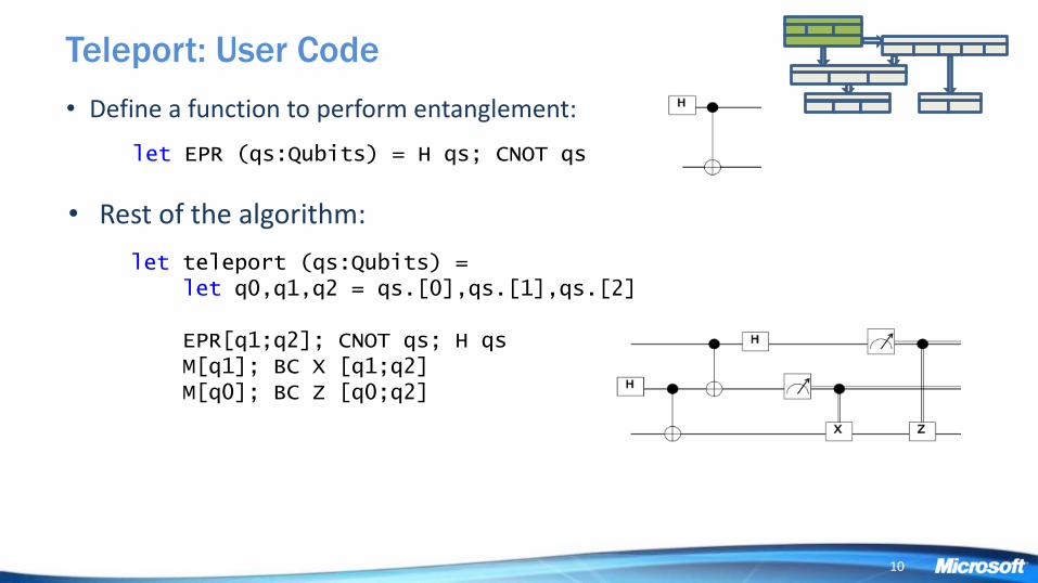
• Define a function to perform entanglement:

Teleport: User Code

let EPR (qs:Qubits) = H qs; CNOT qs

• Rest of the algorithm:

let teleport (qs:Qubits) = let q0,q1,q2 = qs.[0],qs.[1],qs.[2] EPR[q1;q2]; CNOT qs; H qs M[q1]; BC X [q1;q2] M[q0]; BC Z [q0;q2]

10

Teleport: Full Circuit

let circ2 = circ.Fold() circ2.Render(“teleport.svg")

let teleport (qs:Qubits) = let qs' = qs.Tail // Skip first qubit Label >!< (["Src";"|0>";"|0>"],qs) // Label the first 3 qubits EPR qs'; CNOT qs; H qs // EPR 1,2, then CNOT 0,1 and H 0 M qs'; BC X qs' // Conditionally apply X M qs ; BC Z !!(qs,0,2) // Conditionally apply Z Label "Dest" !!(qs,2) // Label output

11

Teleport: Running the code loop N times: … create 3 qubits … init the first one to a random state … print it out teleport qs … print out the result

0:0000.0/Initial State: ( 0.3735-0.2531i)|0>+( -0.4615-0.7639i)|1> 0:0000.0/Final State: ( 0.3735-0.2531i)|0>+( -0.4615-0.7639i)|1> (bits:10) 0:0000.0/Initial State: ( -0.1105+0.3395i)|0>+( 0.927-0.1146i)|1> 0:0000.0/Final State: ( -0.1105+0.3395i)|0>+( 0.927-0.1146i)|1> (bits:11) 0:0000.0/Initial State: ( -0.3882-0.2646i)|0>+( -0.8092+0.3528i)|1> 0:0000.0/Final State: ( -0.3882-0.2646i)|0>+( -0.8092+0.3528i)|1> (bits:01) 0:0000.0/Initial State: ( 0.2336+0.4446i)|0>+( -0.8527+0.1435i)|1> 0:0000.0/Final State: ( 0.2336+0.4446i)|0>+( -0.8527+0.1435i)|1> (bits:10) 0:0000.0/Initial State: ( 0.9698+0.2302i)|0>+(-0.03692+0.0717i)|1> 0:0000.0/Final State: ( 0.9698+0.2302i)|0>+(-0.03692+0.0717i)|1> (bits:11) 0:0000.0/Initial State: ( -0.334-0.3354i)|0>+( 0.315-0.8226i)|1> 0:0000.0/Final State: ( -0.334-0.3354i)|0>+( 0.315-0.8226i)|1> (bits:01)

12

Gate Definition: Standard

/// <summary> /// Controlled NOT gate /// </summary> /// <param name="qs"> Use first two qubits for gate</param> [<LQD>] let CNOT (qs:Qubits) = let gate = Gate.Build("CNOT",fun () -> new Gate( Name = "CNOT", Help = "Controlled NOT", Mat = CSMat(4,[(0,0,1.,0.);(1,1,1.,0.); (2,3,1.,0.);(3,2,1.,0.)]), Draw = "\\ctrl{#1}\\go[#1]\\targ" )) gate.Run qs

13

Teleport: Circuit Compilation

let ket = Ket(3) let circ = Circuit.Compile teleport ket.Qubits circ.Dump showLogInd 0

SEQ APPLY GATE H is a (Normal) 0.7071 0.7071 0.7071-0.7071 WIRE(Id:1) APPLY GATE CNOT is a Controlled NOT (Normal) 1 0 0 0 0 1 0 0 0 0 0 1 0 0 1 0 WIRE(Id:1) WIRE(Id:2) APPLY GATE CNOT is a Controlled NOT (Normal) 1 0 0 0 0 1 0 0 0 0 0 1 0 0 1 0 WIRE(Id:0) WIRE(Id:1) APPLY GATE H is a (Normal) 0.7071 0.7071 0.7071-0.7071 WIRE(Id:0)

APPLY GATE Measure is a Collapse State (Measure) 1 0 0 1 WIRE(Id:1) Modify GATE BitContol is a Bit control Qubit operator (BitOne) 0 1 1 0 WIRE(Id:1) WIRE(Id:2) APPLY GATE X is a Pauli X flip (Normal) 0 1 1 0 WIRE(Id:2) APPLY GATE Measure is a Collapse State (Measure) 1 0 0 1 WIRE(Id:0) Modify GATE BitContol is a Bit control Qubit operator (BitOne) 1 0 0 -1 WIRE(Id:0) WIRE(Id:2) APPLY GATE Z is a Pauli Z flip (Normal) 1 0 0 -1 WIRE(Id:2)

14

Fully Entangled: Simple Version

let entangle (qs:Qubits) = H qs; let q0 = qs.Head for q in qs.Tail do CNOT[q0;q] M >< qs

0:0000.0/#### Iter 0 [ 0.2030]: 0000000000000 0:0000.0/#### Iter 1 [ 0.1186]: 0000000000000 0:0000.0/#### Iter 2 [ 0.0895]: 0000000000000 0:0000.0/#### Iter 3 [ 0.0749]: 0000000000000 0:0000.0/#### Iter 4 [ 0.0664]: 1111111111111 0:0000.0/#### Iter 5 [ 0.0597]: 0000000000000 0:0000.0/#### Iter 6 [ 0.0550]: 1111111111111 0:0000.0/#### Iter 7 [ 0.0512]: 0000000000000 0:0000.0/#### Iter 8 [ 0.0484]: 0000000000000 0:0000.0/#### Iter 9 [ 0.0463]: 0000000000000 0:0000.0/#### Iter 10 [ 0.0446]: 0000000000000 0:0000.0/#### Iter 11 [ 0.0432]: 1111111111111 0:0000.0/#### Iter 12 [ 0.0420]: 0000000000000 0:0000.0/#### Iter 13 [ 0.0410]: 0000000000000 0:0000.0/#### Iter 14 [ 0.0402]: 0000000000000 0:0000.0/#### Iter 15 [ 0.0399]: 0000000000000 0:0000.0/#### Iter 16 [ 0.0392]: 1111111111111 0:0000.0/#### Iter 17 [ 0.0387]: 1111111111111 0:0000.0/#### Iter 18 [ 0.0380]: 0000000000000 0:0000.0/#### Iter 19 [ 0.0374]: 1111111111111

15

Fully Entangled: Parallel Version

48 time steps 10 time steps

16










17

Circuit for Shor’s algorithm using 2n+3 qubits – Stéphane Beauregard

Largest we’ve done:

14 bits (factoring 8193)

~1/2 Million Gates

18

Shor’s algorithm: Modular Adder

As defined in:

Circuit for Shor’s

algorithm using 2n+3 qubits

– Stéphane Beauregard

19

Shor’s algorithm results

N f1 f2 coPrime n Qubits min total

507 3 169 68 9 21 2.35

969 3 323 109 10 23 40.75

975 3 325 697 10 23 32.62

981 3 327 248 10 23 44.28

985 5 197 813 10 23 36.22

987 21 47 190 10 23 42.99

993 3 331 892 10 23 36.48

999 9 111 140 10 23 37.44

1001 11 91 288 10 23 39.75

1011 337 3 622 10 23 39.75

1023 3 341 169 10 23 36.53

1995 7 285 1397 11 25 273.63

2005 5 401 483 11 25 263.94

2013 3 671 1960 11 25 270.72

2019 3 673 533 11 25 256.2

2025 9 225 1792 11 25 267.78

2031 3 677 1640 11 25 267.4

2035 5 407 1281 11 25 261.74

2041 13 157 649 11 25 262.29

2043 9 227 1009 11 25 268.68

4047 3 1349 3251 12 27 2200

4053 3 1351 425 12 27 1858

4061 31 131 150 12 27 1931

4063 17 239 832 12 27 2108

4065 15 271 1219 12 27 2278

4071 3 1357 3670 12 27 2073

4077 3 1359 2111 12 27 2562

4081 7 583 1560 12 27 1361

4083 3 1361 3059 12 27 2268

4089 87 47 958 12 27 2247

4095 3 1365 2972 12 27 2393

8189 19 431 6803 13 29 7455

N f1 f2 coPrime n Qubits min total

45 9 5 8 6 15 0.12

51 17 3 8 6 15 0.09

55 5 11 24 6 15 0.14

57 19 3 52 6 15 0.11

63 3 21 23 6 15 0.13

63 3 21 58 6 15 0.22

65 5 13 21 7 17 0.13

69 3 23 19 7 17 0.14

69 3 23 10 7 17 0.24

85 5 17 49 7 17 0.2

99 9 11 53 7 17 0.2

105 35 3 94 7 17 0.18

115 5 23 51 7 17 0.2

117 3 39 59 7 17 0.22

201 3 67 194 8 19 0.49

203 7 29 43 8 19 0.47

207 9 23 169 8 19 0.77

213 3 71 92 8 19 0.68

219 3 73 7 8 19 0.64

237 3 79 211 8 19 0.83

245 7 35 57 8 19 0.89

247 19 13 184 8 19 0.88

249 3 83 29 8 19 0.61

255 5 51 236 8 19 0.86

459 9 51 224 9 21 1.84

465 15 31 136 9 21 2.06

469 7 67 111 9 21 2.3

473 11 43 111 9 21 1.39

475 95 5 286 9 21 1.53

477 9 53 250 9 21 2.64

485 5 97 93 9 21 1.83

501 3 167 274 9 21 1.99

20







(Pham, Svore) • Classically simulating adiabatic algorithms (Hastings, Freedman) • Computational Complexity (Hastings, Freedman)


21

QECC Gate Definition: Steane7 prep /// <summary> /// Steane7 prep gate (create logical |0>). /// </summary> /// <param name="qs"> Physical qubits to use</param> [<LQD>]

let prep (qs:Qubits) =

let nam = "S7_Prep"

let nam2= "S7\nPrep"

let gate (qs:Qubits) =

// Create logical |0> prep circuit

let op (qs:Qubits) =

let xH i = H [qs.[i]]

let xC i j = CNOT [qs.[i];qs.[j]]

xH 6; xC 6 3; xH 5; xC 5 2; xH 4

xC 4 1; xC 5 3; xC 4 2; xC 6 0; xC 6 1

xC 5 0; xC 4 3

Gate.Build(nam,fun () ->

new Gate(

Qubits = qs.Length,

Name = nam,

Help = "Prepare logical 0 state",

Draw = sprintf "\\multigate{#%d}{%s}“ (qs.Length-1) nam, Op = WrapOp op

))

(gate qs).Run qs

22

QECC Gate Definition: Steane7 syndrome

23

Full Teleport Circuit in a Steane7 Code

24

Encode

Hadamard CNOT

Syndrome 1 Syndrome 2 Syndrome 3

CNOT Measure

Stabilizers

let tele1 (qs:Qubits) = X qs; teleport qs; M [qs.[2]] let tgtC1 = Circuit.Compile tele1 qs

let s7 = Steane7(tgtC1)

let s7C = s7.Circuit

let stab = Stabilizer(s7c,s7.Ket)

stab.Run() let bit0,dist0 = s7.Log2Phys 0 |> s7.Decode

let bit1,dist1 = s7.Log2Phys 1 |> s7.Decode

let bit2,dist2 = s7.Log2Phys 2 |> s7.Decode

> LIQUiD /l __QECC

0:0000.0/LOOP[Zer0]: InjectedXYZ(0,0,0) Fixes=0 (Zero, One,Zero) dist=(0,0,0)

0:0000.0/LOOP[Zer1]: InjectedXYZ(0,1,0) Fixes=2 ( One,Zero,Zero) dist=(0,0,0)

0:0000.0/LOOP[Zer2]: InjectedXYZ(0,1,1) Fixes=2 (Zero,Zero,Zero) dist=(0,0,0)

0:0000.0/LOOP[Zer3]: InjectedXYZ(0,1,1) Fixes=0 (Zero,Zero,Zero) dist=(0,0,1)






0:0000.1/LOOP[Zer9]: InjectedXYZ(0,1,0) Fixes=1 ( One, One,Zero) dist=(0,0,0)

0:0000.1/LOOP[One0]: InjectedXYZ(0,0,0) Fixes=0 (Zero, One, One) dist=(0,0,0)


0:0000.1/LOOP[One2]: InjectedXYZ(0,0,1) Fixes=1 ( One, One, One) dist=(0,0,0)

0:0000.1/LOOP[One3]: InjectedXYZ(0,1,1) Fixes=3 (Zero,Zero, One) dist=(0,0,0)

0:0000.1/LOOP[One4]: InjectedXYZ(0,0,1) Fixes=1 ( One, One, One) dist=(0,0,0)

0:0000.1/LOOP[One5]: InjectedXYZ(0,0,1) Fixes=1 ( One,Zero, One) dist=(0,0,0)





-X................ZZZ....ZZZ -XX................Z......Z. -XXX................Z......Z -X..X............ZZZZ....ZZZ +.X..X.........Z..Z.Z....Z.Z +.XX.XX.........Z.ZZ.....ZZ. +..X..XX...........ZZ.....ZZ +.X..X..X.........Z.Z....Z.Z +.XX.XX..X........ZZ.....ZZ. -X..X.....X.......ZZZ....ZZZ -X.XX.X....X......Z......Z.. -XX.XX......X......Z......Z. -XXXXXX......X......Z......Z +..X..........X............. +.X..ZZZZ..ZZ..X............ +.XX..ZZ.Z.Z.Z..X........... +X..Z.....ZZZZ...X.......... -YZX...........ZZZY......... -YXZ..........Z.ZZ.Y........ +YYY..........ZZ.Z..Y....... +....................X...... +.....................X..... +......................X.... +.......................X... +ZZ............ZZZZ...XXXX.. +.ZZ..........ZZ..ZZ.XX..XX. +..Z..........Z.Z.Z.ZX.X.X.X ----------------------------

+ZZ.ZZ.........ZZZZ......... +.ZZ.ZZ.......ZZ..ZZ........ +..Z..Z.......Z.Z.Z.Z....... +...Z.....ZZZZ.............. +....ZZZZ..ZZ............... +.....ZZ.Z.Z.Z.............. +......Z.................... +.......Z................... +........Z.................. +.........Z................. +..........Z................ +...........Z............... +............Z.............. +.............Z............. +..............Z............ -...............Z........... -................Z.......... +.................Z......... +..................Z........ -...................Z....... +....................Z....ZZ +.....................Z..Z.Z +......................Z.ZZ. +.......................ZZZZ -........................ZZZ -.........................Z. +..........................Z

Final Tableau: (after Gaussian)

25










26

Noise(circ:Circuit,ket:Ket,models:NoiseModels) type NoiseModel = { gate: string // Gate name (ending with "*" for wildcard match) maxQs: int // Max qubits that gate uses time: float // floating duration of gate (convention Idle = 1.0) func: NoiseFunc // Noise Model to execute gateEvents: NoiseEvents // Stats for normal gates ecEvents: NoiseEvents // Stats for EC gates } member n.DampProb // Get/Set damping probability on a qubit

Advanced Noise Modeling

27

0

0.2

0.4

0.6

0.8

1

0 20 40 60 80

Mea

sure

mt

Pro

bab

ility

Time

Two Qubits H01N01

State 00

State 01

State 10

State 11

Unitary Noise

Non-Unitary Noise









28

• Some gates may not be available in a fault-tolerant physical implementation.

• Need to efficiently decompose a quantum circuit into fault-tolerant, implementable gates.

Approximation of Quantum Circuits

29

Single-qubit Gate Decomposition

30

http://arxiv.org/abs/1303.1411



Single-qubit Gate Decomposition

31

Bocharov, Gurevich, Svore, 2013; arXiv:1303.1411










32

Faster Phase Estimation

33




•

Faster Phase Estimation

34







(Pham, Svore) • Classically simulating adiabatic algorithms (Hastings,

Freedman, Troyer, Wecker) • Computational Complexity (Hastings, Freedman)


35

• Bimodal histogram of success rates for D-Wave and the simulated quantum annealer

• D-Wave One is a thermal annealer

• D-Wave One is consistent with a simulated quantum annealer

36 Matthias Troyer

DPHYS Department of Physics

Institute for Theoretical Physics

36

Classical annealer Simulated

quantum annealer

D-Wave One










(Pham, Svore) • Classically simulating adiabatic algorithms (Hastings, Freedman,



37

• Very interesting molecules can be modeled with high fidelity in less than 1000 qubits

• Opportunity to design new materials, including ones for next generation QC (bootstrapping)

• Fits naturally into the gate and circuit model that we’re using

Hamiltonians (Fermion Model)

http://arxiv.org/abs/quant-ph/0604193

38




// Invoke by picking which test to run: // Liquid /s H2O.fsx Main(245)

module Script = // The script module allows for incremental loading let dic = Dictionary<string,string>() // Parameters to Fermion dic.["Test"] <- "245" // Test to process dic.["Bits"] <- "20" // Bit accuracy dic.["Trotter"]<- "128" // Trotter number dic.["Thresh"] <- "-83.7" // Max threshold to accept as an answer (w/o NR) dic.["Emin"] <- "-85.1" // Min possible energy (without nuclear repulsion) dic.["Emax"] <- "-35.0" // Max possible energy (without nuclear repulsion) dic.["Ecnt"] <- "10" // Electron count dic.["SOs"] <- "14" // Spin orbitals dic.["Parity"] <- "1" // Enforce parity between rows and columns? dic.["Diff"] <- "0" // Spin Up/Down enforced difference (default is none) dic.["HalfUp"] <- "0" // These are interleaved dic.["Single"] <- "1" // Use single Unitary? dic.["Preps"] <- "[1;2;3;4;5;6;7;8;9;10]" // Prepared states to start in (list of lists) dic.["Alter"] <- "0.0" // Alter angle by factor (0.0<- "don't alter) dic.["AltCnt"] <- "1" // Count of altered circuits to use let data = [| "tst=0 info=95.5,1.820 nuc=9.162349762 Ehf=-74.962999077 00=-32.696652545 ...

Defining the Water Molecule

39

Water

Spin Orbitals 14 168

SO Constants 434 6.4E+06

Primitive Gates 3.4E+04 5.E+08

Qubits 15 169

9 bit accuracy 2.E+07 3.E+11

Sampling 9.E+08 1.E+13

Trotterization 9.E+11 1.E+16

Full Graph 9.E+13 1.E+18

SK Rotations 9.E+15 1.E+20

QECC 9.E+18 1.E+23

Ground State Fixed Angle/Bond Len

RHF DFT EigenSolver

Egs -74.965832 -76.399089 -74.980538 -74.9906579 -74.990725

Angle 100.5 102 101.5 100 100

Bond Len 1.86 1.84 1.87 1.9 1.9

40

Multi-Resolution Trotterization

41







(Pham, Svore) • Classically simulating adiabatic algorithms (Hastings, Freedman,



42

•

Adiabatic Solution of the Hubbard model

General Circuit Kinetic Energy Measurement

Fermionic Permutations

Basis

Change

See: d-wave resonating valence bond states of fermionic atoms in optical lattices 43

Thank You!

Backup Slides

Quantum Algorithms

Quantum Circuits

QuArC Research Activities

46

•

A little bit of F# syntax

47

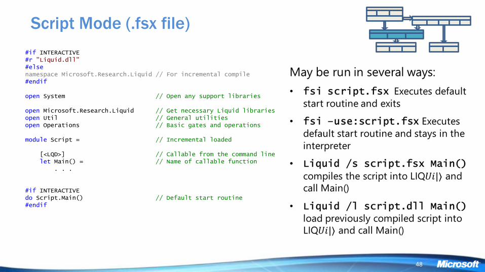
Script Mode (.fsx file)

#if INTERACTIVE #r "Liquid.dll" #else namespace Microsoft.Research.Liquid // For incremental compile #endif open System // Open any support libraries open Microsoft.Research.Liquid // Get necessary Liquid libraries open Util // General utilities open Operations // Basic gates and operations module Script = // Incremental loaded [<LQD>] // Callable from the command line let Main() = // Name of callable function . . . #if INTERACTIVE do Script.Main() // Default start routine #endif

48

•

Library of Gates

M qs; BC (Adj T) qs

49

Fully Entangled: Parallel Version

// Parallel entanglement let entangle (qs':Qubits) = // Do the heads of the groups H qs' for i in 5..5..qs'.Length-1 do CNOT !!(qs',0,i) // Do each group of upto 4 let rec doGroup (qs:Qubits) = let len = qs.Length if len >= 2 then let lst = if len <= 5 then len-1 else 4 for i in [1..lst] do CNOT !!(qs,0,i) Seq.skip (lst+1) qs |> Seq.toList |> doGroup doGroup qs‘ // Measure all the qubits M >< qs’

0:0000.0/========== Entangle 20 qubits, 10 times ============= 0:0000.0/Starting 20 qubits... 0:0000.0/ Entangle Mem: Priv= 110/ 585 MB WS= 59/ 59 MB 0:0000.0/ Measure Mem: Priv= 78/ 585 MB WS= 27/ 60 MB 0:0000.0/#### Iter 0 [ 2.1942]: 00000000000000000000 0:0000.1/#### Iter 1 [ 2.1146]: 00000000000000000000 0:0000.1/#### Iter 2 [ 2.0675]: 00000000000000000000 0:0000.1/#### Iter 3 [ 2.0585]: 11111111111111111111 0:0000.2/#### Iter 4 [ 2.0419]: 00000000000000000000 0:0000.2/#### Iter 5 [ 2.0535]: 11111111111111111111 0:0000.2/#### Iter 6 [ 2.0639]: 11111111111111111111 0:0000.3/#### Iter 7 [ 2.0638]: 00000000000000000000 0:0000.3/#### Iter 8 [ 2.0618]: 00000000000000000000 0:0000.4/#### Iter 9 [ 2.0676]: 11111111111111111111 0:0000.4/Got 4 ones (40.000%)

50

<?xml version="1.0" encoding="utf-8"?> <Ensemble Default=“H2O"> <Pars> <Exe>\\machine-00\Liquid\Liquid.exe</Exe> <Host>machine-00</Host> <Host>machine-01</Host> <Host>machine-02</Host> <Host>machine-03</Host> <Host>machine-04</Host> <Host>machine-05</Host> <Host>machine-06</Host> <Host>machine-07</Host> <Host>machine-08</Host> <Host>machine-09</Host> </Pars> <H2O Count="546" Script="\\machine-00\Liquid\H2O.fsx"> <Cmd Range="0,1,545">Main(%d)</Cmd> </H2O> </Ensemble>

Simulating Water on a LAN or Cluster

Run with: Liquid /e H2O

51

Fully Entangled: Ensemble computation

0:0000.2/*1 ( 1 0.1%) 1:0000.4/*3*3*3*3*3*3*3*3*3*3*3*3*4*3*3*3*3*3*3*3 ( 60 6.1%) 2:0000.6/*6*6*6*6*6*6*6*6*6*6*6*7*6*6*6*6*6*6*6*6 ( 60 12.1%) 3:0000.8/*9*9*9*9*9*9*10*9*9*9*9*9*9*9*9*9*9*9*9*9 ( 60 18.1%) 1:0001.0/*12*12*12*12*12*12*13*12*12*12*12*12*12*12*12*12*12*12*12*12 ( 60 24.1%) 3:0001.2/*15*15*15*15*15*15*15*15*15*15*15*16*15*15*15*15*15*15*15*15 ( 60 30.1%) 4:0001.4/*18*18*18*18*18*18*18*18*18*18*18*19*18*18*18*18*18*18*18*18 ( 60 36.1%) 5:0001.6/*21*21*21*21*21*21*21*21*21*21*21*22*21*21*21*21*21*21*21*21 ( 60 42.1%) 6:0001.8/*24*24*24*24*24*24*24*24*24*24*24*25*24*24*24*24*24*24*24*24 ( 60 48.1%) 1:0002.0/*27*27*27*27*27*27*27*27*27*27*27*28*27*27*27*27*27*27*27*27 ( 60 54.1%) 7:0002.2/*30*30*30*30*30*30*30*30*30*30*30*31*30*30*30*30*30*30*30*30 ( 60 60.1%) 0:0002.4/*33*33*33*33*33*33*33*33*33*33*33*34*33*33*33*33*33*33*33*33 ( 60 66.1%) 8:0002.6/*36*36*36*36*36*36*36*36*36*36*36*37*36*36*36*36*36*36*36*36 ( 60 72.1%) 0:0002.8/*39*39*39*39*39*39*39*39*39*39*39*40*39*39*39*39*39*39*39*39 ( 60 78.1%) 9:0003.0/*42*42*42*42*42*42*42*42*42*42*42*43*42*42*42*42*42*42*42*42 ( 60 84.1%) a:0003.2/*45*45*45*45*45*45*45*45*45*45*45*46*45*45*45*45*45*45*45*45 ( 60 90.1%) 4:0003.3/*48*48*48*48*48*48*48*48*48*48*48*48*48*48*48*48*48*48*48*48 ( 59 96.0%) b:0003.4/ 48 48 48 48 48 48 48*49 48 48*50 48 48*49*49*49 48*49 48 48 ( 7 96.7%) c:0003.5/ c:0003.5/===== 1000 Runs of 22 qubits each across 60 silos with 8 threads each ===== c:0003.5/Final tally: All 0s = 489 (48.90%), All 1s = 511 (51.10%)

1000 Runs of 22 Entangled

Qubits in 3 ½ minutes

52

• Built-in Hamiltonian simulator for doing spin-glass models

• Able to reproduce ground states for published D-Wave examples

• Built-in test for doing ferromagnetic chains

• Here’s what the circuit looks like…

• Just added a decoherence model and entanglement entropy measurement (thanks to Andrew Das Sarma)

Hamiltonians (Spin Model)

in conjunction with Matthias Troyer, ETH Zurich 53

Whitfield et al: http://arxiv.org/abs/1001.3855

54


• Output generated on

cluster of 20 machines

in ~1 minute

Quantum Chemistry Simulation Results

Lanyon et al: http://arxiv.org/abs/0905.0887

55


• Simple STO-3g basis (for comparison with simulation)

Water

56

•

Machine Learning - Traveling Salesman

57

•

Quantum Walks (PageRank example)

58

Adiabatic quantum algorithm for search engine ranking

Garnerone, Zanardi, Lidar (arXiv.org/1109.6546)

59

Documents

Quantum Computing Research at Microsoft · To design real-world quantum algorithms for implementation on small-, medium-, and large-scale quantum computers To design quantum circuits