QUANTUM COMPUTING CLASSICAL PHYSICS - …math.ucsd.edu/~dmeyer/research/publications/qccp/qccp.pdf12 August 2001 quant-ph/0111069 QUANTUM COMPUTING CLASSICAL PHYSICS David A. Meyer

12 August 2001quant-ph/0111069

QUANTUM COMPUTING CLASSICAL PHYSICS

David A. Meyer

Project in Geometry and PhysicsDepartment of Mathematics

University of California/San DiegoLa Jolla, CA 92093-0112 [email protected]

ABSTRACT

In the past decade quantum algorithms have been found which outperform the best classicalsolutions known for certain classical problems as well as the best classical methods knownfor simulation of certain quantum systems. This suggests that they may also speed up thesimulation of some classical systems. I describe one class of discrete quantum algorithmswhich do so—quantum lattice gas automata—and show how to implement them efficientlyon standard quantum computers.

2001 Physics and Astronomy Classification Scheme: 03.67.Lx. 05.10.-a.2000 American Mathematical Society Subject Classification: 81P68, 65Z05.Key Words: quantum lattice gas automata, quantum simulation, quantum Fourier trans-

form.

Expanded version of an invited talk presented at the NATO Advanced Workshop DiscreteSimulation of Fluid Dynamics: New Trends, New Perspectives, Cargese, France, 2–6 July2001.

1

Quantum computing classical physics David A. Meyer

1. Introduction

Quantum computing originated with Feynman’s observation that quantum systems arehard to simulate on classical computers, but that they might be easier to simulate if onehad a computer which could be operated quantum mechanically [1]. Developments dur-ing the subsequent two decades have not only supported this observation [2–8], but havealso demonstrated that quantum computers would—if they existed—solve certain classicalproblems like factoring more efficiently than is possible on classical computers running thebest classical algorithms known [9]. This raises a natural question [10–12]: Might quan-tum computers help with the simulation of classical systems? Or more specifically, giventhe focus of this workshop, could quantum computers efficiently simulate fluid dynamics?Without answering the specific question, in this paper I try to explain why the answerto the general question may be ‘yes’, and along the way explain some of the quantumalgorithmic tricks which seem likely to be useful in future investigations of these questions.

I begin by (very) rapidly introducing the ideas of quantum computation in §2. Fora complete presentation, see [13]. In §3 I describe one approach to simulating quantumsystems—quantum lattice gas automata (QLGA) [14]—and then in §4 explain a connectionwith simulation of classical systems. The crucial issue is the relative complexity of quan-tum and classical algorithms; so §5 contains a detailed analysis for one specific problem,including some new results on implementing QLGA algorithms on ‘standard’ quantumcomputers. I conclude with a brief discussion in §6.

2. Quantum computers

The possible states of a classical computer are (very long) bit strings b1 . . . bn ∈ {0, 1}n. Aparticular computation proceeds via a sequence of maps to new bit strings: b′1 . . . b′n, . . .. Afundamental result, which contributed directly to the conceptual development of quantumcomputation, is that any classical computation can be made to be reversible [15], i.e., thesemaps can be chosen to be permutations on the space of states. Quantum computation canthen be understood as a generalization of classical computation: The possible states of aquantum computer are superpositions of bit strings

∑ab1...bn |b1 . . . bn〉 ∈ (C2)⊗n (each C2

tensor factor is called a quantum bit or qubit), where∑|ab1...bn |2 = 1 so that the norm-

squared of each amplitude ab1...bn ∈ C is the probability that the state |b1 . . . bn〉 is observedif the quantum system is measured in this ‘computational basis’. A particular quantumcomputation proceeds via a sequence of unitary maps to new states

∑a′b1...bn|b1 . . . bn〉,

. . .. This much is a generalization of classical reversible computation since permutationsare unitary maps, and each classical state is an allowed quantum state. The differenceis that the final state is not directly available; it can only be sampled according to theprobabilities given by the norm-squared of the amplitudes.

To evaluate the computational complexity of an algorithm, either classical or quan-tum, we must specify a set of elementary operations, the number of which used duringthe computation quantifies the complexity. If we allow arbitrary permutations classically,or arbitrary unitary transformations quantum mechanically, any state can be reached from

2


Xa

a

b

a

b

c

a+1

a

b+a

a

b

c+ab

NOT

C-NOT

C-C-NOT

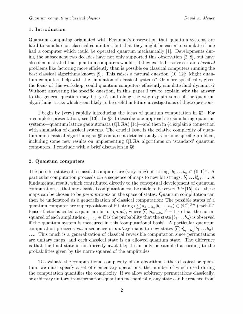
Figure 1. A universal set of classical reversiblegates. Inputs are on the left; outputs are on theright. + denotes addition mod 2.

any other state in a single step—these areclearly not reasonable models of compu-tation. Instead, consider the ‘gate opera-tions’ shown in Fig. 1: NOT, C-NOT and C-

C-NOT (‘C’ abbreviates ‘CONTROLLED’).Each of these is a permutation on the setof bit strings, and Toffoli [16] has shownthat this set of three gates is universal forclassical computation, in the sense thatany (reversible) boolean operation can bedecomposed as a sequence of these gates—which by Bennett’s result [15] suffices foruniversality. Each of these gates can beextended by linearity to a unitary map on(C2)⊗n, acting non-trivially only on a sub-set of 1, 2, or 3 qubits, and thus can alsobe used as a quantum gate. (Tradition-ally the quantum NOT gate is denoted byσx or X.) Two other quantum gates which are particularly useful act on single qubits:

H =1√2

(1 11 −1

)and Rω =

(1 00 ω

),

the ‘Hadamard transform’ and phase ω rotation, respectively. These matrices have beenexpressed in the computational basis; thus

H|0〉 7→ 1√2

(|0〉+ |1〉)

H|1〉 7→ 1√2

(|0〉 − |1〉).

C-NOT and Rω for ω = eiθ with θ = cos−1 35 form a universal set of gates for quantum

computation [17].

As we noted earlier, any array of (reversible) classical gates can be simulated by somearray of quantum gates. The remarkable fact is that in some cases fewer gates are requiredquantum mechanically. The following example is the smallest version of the Deutsch-Jozsa[18] and Simon [19] problems:

EXAMPLE. Given a function f : {0, 1} → {0, 1}, we would like to evaluate f(0) XOR

f(1). The function is accessed by calls which have the effect of taking classical states (x, b)to(x, b ⊕ f(x)

)where ⊕ denotes addition mod 2. This is a reversible operation and thus

also defines a unitary transformation on a pair of qubits: f-C-NOT. Classically, this gatemust be applied at least twice (once with x = 0 and once with x = 1) in any algorithmwhich outputs f(0) XOR f(1) correctly with probability greater than 1

2 (assuming a uniform

3


distribution on the possible functions). Quantum mechanically we can exploit interferenceto do better, applying the operation only once. Suppose the system is initialized in thestate |0〉 ⊗ |0〉. Then apply the following sequence of unitary operations:

|0〉 ⊗ |0〉 H⊗HX7−−−→1∑x=0

12|x〉 ⊗ (|0〉 − |1〉)

fCNOT7−−−→1∑x=0

12

(−1)f(x)|x〉 ⊗ (|0〉 − |1〉)

H⊗I27−−−→1∑

x,y=0

12√

2(−1)f(x)(−1)xy|y〉 ⊗ (|0〉 − |1〉)

=1√2|f(0) XOR f(1)〉 ⊗ (|0〉 − |1〉).

The first step Fourier transforms the ‘query’ qubit into an equal superposition of |0〉 and|1〉, and initializes the ‘response’ qubit into a state which will create the phase (−1)f(x)

in the second step. The third step Fourier transforms the query qubit again, creating theinterference which ensures that subsequently measuring the query qubit outputs f(0) XOR

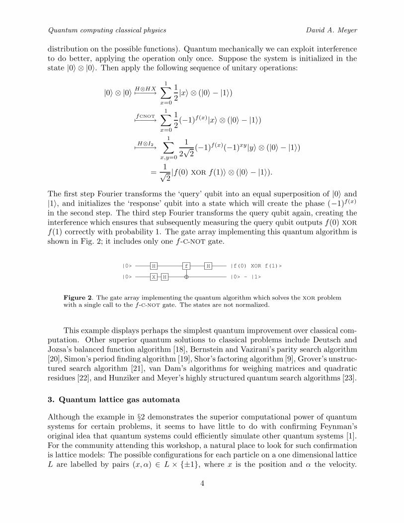
f(1) correctly with probability 1. The gate array implementing this quantum algorithm isshown in Fig. 2; it includes only one f-C-NOT gate.

X

H

H

f H

|0>

|0> |f(0) XOR f(1)>

|0> - |1>

Figure 2. The gate array implementing the quantum algorithm which solves the XOR problemwith a single call to the f-C-NOT gate. The states are not normalized.

This example displays perhaps the simplest quantum improvement over classical com-putation. Other superior quantum solutions to classical problems include Deutsch andJozsa’s balanced function algorithm [18], Bernstein and Vazirani’s parity search algorithm[20], Simon’s period finding algorithm [19], Shor’s factoring algorithm [9], Grover’s unstruc-tured search algorithm [21], van Dam’s algorithms for weighing matrices and quadraticresidues [22], and Hunziker and Meyer’s highly structured quantum search algorithms [23].

3. Quantum lattice gas automata

Although the example in §2 demonstrates the superior computational power of quantumsystems for certain problems, it seems to have little to do with confirming Feynman’soriginal idea that quantum systems could efficiently simulate other quantum systems [1].For the community attending this workshop, a natural place to look for such confirmationis lattice models: The possible configurations for each particle on a one dimensional latticeL are labelled by pairs (x, α) ∈ L × {±1}, where x is the position and α the velocity.

4


A classical lattice gas evolution rule consists of an advection stage (x, α) 7→ (x + α,α),followed by a scattering stage. Each particle in a quantum lattice gas automaton (QLGA)[14] exists in states which are superpositions of the classical states: |ψ〉 =

∑ψx,α|x, α〉,

where 1 = 〈ψ|ψ〉 =∑ψx,αψx,α. The evolution rule must be unitary; the most general

with the same form as the classical rule is:∑ψx,α|x, α〉 advect7−−−→

∑ψx,α|x+ α,α〉

scatter7−−−→∑

ψx,αSαα′|x+ α,α′〉,

where the scattering matrix is

S =(

cos s i sin si sin s cos s

).

cos s

i sin s

Figure 3. The general evolution rule for a singleparticle in the one dimensional QLGA.

Let U denote the complete single timestepevolution operator for a single particle,the composition of advection and scatter-ing. Fig. 3 illustrates this quantum evo-lution: at s = 0 it specializes to the clas-sical deterministic lattice gas rule. The∆x = ∆t → 0 limit of this discrete timeevolution is the Dirac equation [14]; the ∆x2 = ∆t→ 0 limit is the Schrodinger equation[24].

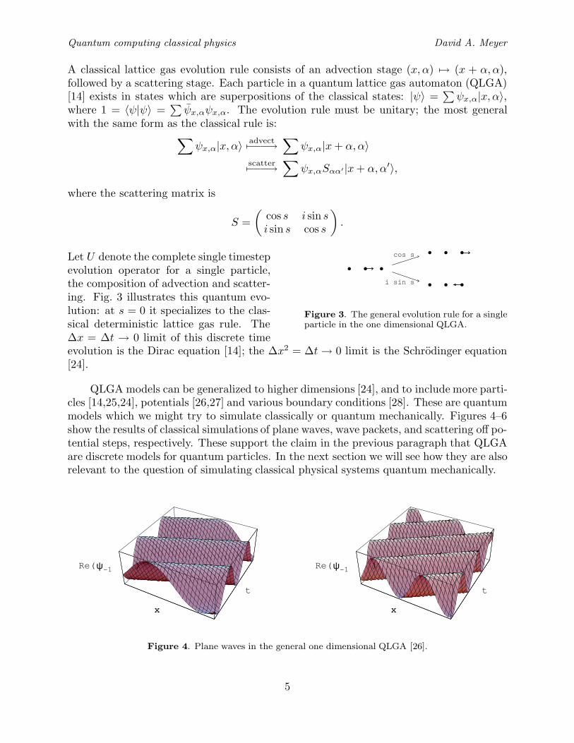
QLGA models can be generalized to higher dimensions [24], and to include more parti-cles [14,25,24], potentials [26,27] and various boundary conditions [28]. These are quantummodels which we might try to simulate classically or quantum mechanically. Figures 4–6show the results of classical simulations of plane waves, wave packets, and scattering off po-tential steps, respectively. These support the claim in the previous paragraph that QLGAare discrete models for quantum particles. In the next section we will see how they are alsorelevant to the question of simulating classical physical systems quantum mechanically.

x

t

x

Re(ψ-1 )

x

t

x

Re(ψ-1 )

Figure 4. Plane waves in the general one dimensional QLGA [26].

5


x

t

x

|ψ|2

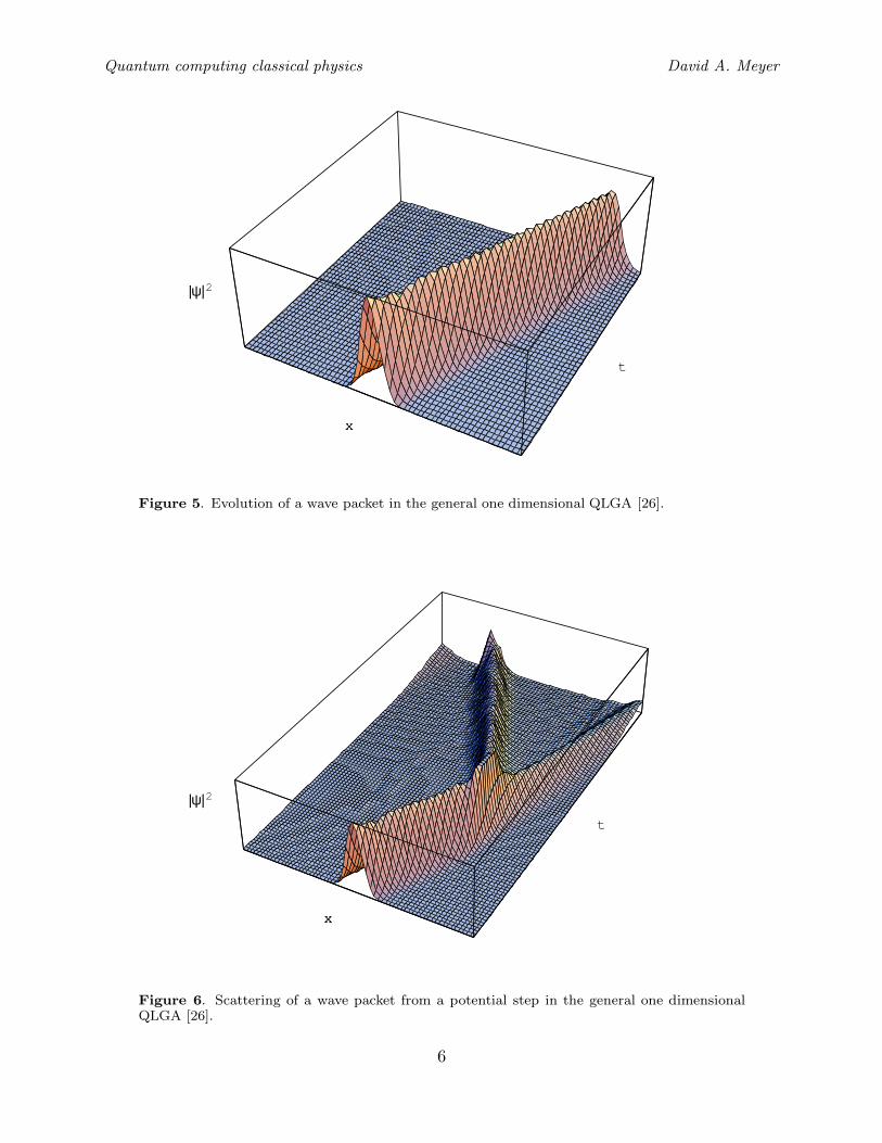
Figure 5. Evolution of a wave packet in the general one dimensional QLGA [26].

x

t

x

|ψ|2

Figure 6. Scattering of a wave packet from a potential step in the general one dimensionalQLGA [26].

6


4. Diffusion

The evolution rule for a single particle QLGA bears some resemblence to a random walk.More precisely, it is the unitary version of a correlated random walk [29,30]—with θ = π/4the analogue of uncorrelated. In Fig. 5, for example, we can see evolution like that of abiased random walk, with a spreading Gaussian distribution. And, in fact, this is as closeas possible—there is no quantum random walk in the sense of local, solely x dependentunitary evolution; the α dependence must be included [31]. (This is not true for quantumprocesses continuous in time [32], which can also be used for computational purposes likethe ones we are considering here [33,34].)

Consequently, there are differences. Diffusion approaches an equilibrium state, in-dependently of the initial condition (on connected spaces). Unitary evolution of a singleparticle QLGA cannot: the distance δ between successive states, defined by cos δ = 〈Uψ|ψ〉is constant, so the evolution of any state which is not an eigenstate of U with eigenvalue1 does not converge. Each state implies a probability distribution on the lattice, given by

Pt(x) = prob(x; t) = |ψx,−1(t)|2 + |ψx,+1(t)|2,

so we can also ask if this converges. In fact, this probability distribution is constant foreach eigenstate |φi〉 of U [26]. But since there exists T ∈ Z>0 such that λTi ∼ 1 for alleigenvalues λi of U , and hence UTψ ∼ ψ, for any initial state such that P1 6= P0, theprobability distribution cannot converge either [35].

Aharonov, Ambainis, Kempe and Vazirani have shown, however, that the time averageof the probability distribution does converge [35]: Expand the initial state |ψ〉 =

∑i ai|φi〉

in terms of the eigenvectors of U . Then U t|ψ〉 =∑

i aiλti|φi〉, so

prob(x, α; t) =∣∣∣∑i

aiλti〈x, α|φi〉

∣∣∣2=∑i,j

aiaj(λiλj)t〈x, α|φi〉〈φj |x, α〉.

Then the time average of the probability is

1T

T−1∑t=0

prob(x, α; t) =∑i,j

aiaj〈x, α|φi〉〈φj |x, α〉1T

T−1∑t=0

(λiλj)t.

For λi 6= λj , the interior sum goes to 0 as T → ∞. This leaves only the terms in thesum for which λi = λj , which are independent of T . Thus the time average converges.In particular, for the one dimensional single particle QLGA, it converges to the uniformdistribution which is the equilibrium distribution for diffusion on one dimensional lattices.That is, by measuring the position at random times we can simulate sampling from theequilibrium distribution of classical diffusion. Although this is not true for all graphs,

7


e.g., the Cayley graph of the nonabelian group S3 [35], we have analyzed one example ofdiscrete quantum simulation of a classical physical process.

5. Computational complexity

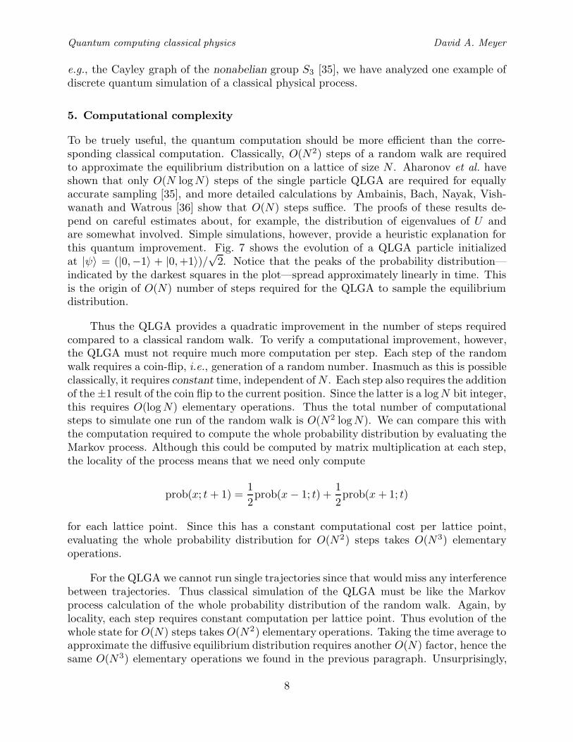
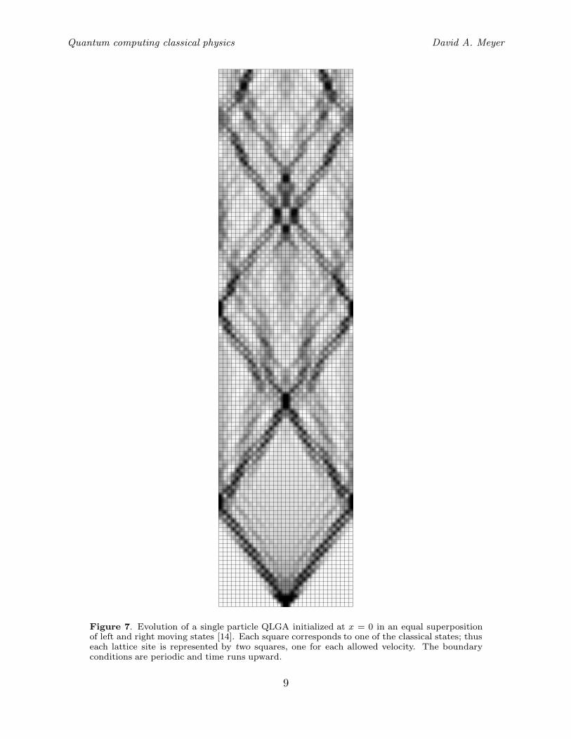
To be truely useful, the quantum computation should be more efficient than the corre-sponding classical computation. Classically, O(N2) steps of a random walk are requiredto approximate the equilibrium distribution on a lattice of size N . Aharonov et al. haveshown that only O(N logN) steps of the single particle QLGA are required for equallyaccurate sampling [35], and more detailed calculations by Ambainis, Bach, Nayak, Vish-wanath and Watrous [36] show that O(N) steps suffice. The proofs of these results de-pend on careful estimates about, for example, the distribution of eigenvalues of U andare somewhat involved. Simple simulations, however, provide a heuristic explanation forthis quantum improvement. Fig. 7 shows the evolution of a QLGA particle initializedat |ψ〉 = (|0,−1〉 + |0,+1〉)/

√2. Notice that the peaks of the probability distribution—

indicated by the darkest squares in the plot—spread approximately linearly in time. Thisis the origin of O(N) number of steps required for the QLGA to sample the equilibriumdistribution.

Thus the QLGA provides a quadratic improvement in the number of steps requiredcompared to a classical random walk. To verify a computational improvement, however,the QLGA must not require much more computation per step. Each step of the randomwalk requires a coin-flip, i.e., generation of a random number. Inasmuch as this is possibleclassically, it requires constant time, independent ofN . Each step also requires the additionof the ±1 result of the coin flip to the current position. Since the latter is a logN bit integer,this requires O(logN) elementary operations. Thus the total number of computationalsteps to simulate one run of the random walk is O(N2 logN). We can compare this withthe computation required to compute the whole probability distribution by evaluating theMarkov process. Although this could be computed by matrix multiplication at each step,the locality of the process means that we need only compute

prob(x; t + 1) =12

prob(x− 1; t) +12

prob(x+ 1; t)

for each lattice point. Since this has a constant computational cost per lattice point,evaluating the whole probability distribution for O(N2) steps takes O(N3) elementaryoperations.

For the QLGA we cannot run single trajectories since that would miss any interferencebetween trajectories. Thus classical simulation of the QLGA must be like the Markovprocess calculation of the whole probability distribution of the random walk. Again, bylocality, each step requires constant computation per lattice point. Thus evolution of thewhole state for O(N) steps takes O(N2) elementary operations. Taking the time average toapproximate the diffusive equilibrium distribution requires another O(N) factor, hence thesame O(N3) elementary operations we found in the previous paragraph. Unsurprisingly,

8


Figure 7. Evolution of a single particle QLGA initialized at x = 0 in an equal superpositionof left and right moving states [14]. Each square corresponds to one of the classical states; thuseach lattice site is represented by two squares, one for each allowed velocity. The boundaryconditions are periodic and time runs upward.

9


therefore, we have not discovered a faster classical algorithm for simulating the equilibriumdistribution of diffusion.

S

ADVECT

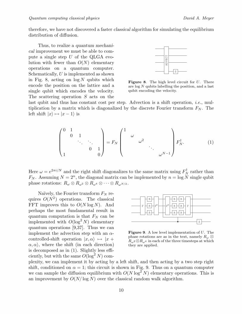
Figure 8. The high level circuit for U . Thereare logN qubits labelling the position, and a lastqubit encoding the velocity.

Thus, to realize a quantum mechani-cal improvement we must be able to com-pute a single step U of the QLGA evo-lution with fewer than O(N) elementaryoperations on a quantum computer.Schematically, U is implemented as shownin Fig. 8, acting on logN qubits whichencode the position on the lattice and asingle qubit which encodes the velocity.The scattering operation S acts on thelast qubit and thus has constant cost per step. Advection is a shift operation, i.e., mul-tiplication by a matrix which is diagonalized by the discrete Fourier transform FN . Theleft shift |x〉 7→ |x− 1〉 is

0 1

0 1. . . . . .

0 11 0

= FN

1

ωω2

. . .ωN−1

F †N . (1)

Here ω = e2πi/N and the right shift diagonalizes to the same matrix using F †N rather thanFN . Assuming N = 2n, the diagonal matrix can be implemented by n = logN single qubitphase rotations: Rω ⊗Rω2 ⊗Rω4 ⊗ · · · ⊗RωN/2 .

S

R

R

R

R

R

R

R

R

R

F F+ F+ F

Figure 9. A low level implementation of U . Thephase rotations are as in the text, namely Rω ⊗Rω2⊗Rω4 in each of the three timesteps at whichthey are applied.

Naıvely, the Fourier transform FN re-quires O(N2) operations. The classicalFFT improves this to O(N logN). Andperhaps the most fundamental result inquantum computation is that FN can beimplemented with O(log2N) elementaryquantum operations [9,37]. Thus we canimplement the advection step with an α-controlled-shift operation |x, α〉 7→ |x +α,α〉, where the shift (in each direction)is decomposed as in (1). Slightly less effi-ciently, but with the sameO(log2 N) com-plexity, we can implement it by acting by a left shift, and then acting by a two step rightshift, conditioned on α = 1; this circuit is shown in Fig. 9. Thus on a quantum computerwe can sample the diffusion equilibrium with O(N log2 N) elementary operations. This isan improvement by O(N/ logN) over the classical random walk algorithm.

10


6. Discussion

We have seen that a classical physics problem—sampling from the equilibrium distributionof a diffusion process—is solvable more efficiently with a quantum computer than witha classical one, in the sense that the QLGA algorithm outperforms the random walkalgorithm. The solution utilizes two of the fundamental quantum speedups: First, thequadratic improvement in the number of steps necessary for a QLGA simulation comparedto a random walk simulation is reminiscent of the quadratic improvement of Grover’squantum search algorithm—which he, in fact, describes as diffusion [21]. Second, theexponential improvement of the quantum Fourier transform over the FFT [9,37] providesa speedup in the advection step. Perhaps the simple problem considered here will inspireapplication of these techniques—or new ones—to speed up computation of other classicalsystems with quantum algorithms. For example, a natural generalization would be toanalyze diffusion in a potential, for which a QLGA simulation has already been shownto evolve the mean of the distribution quadratically faster than does a classical (biased)random walk, in certain cases [30]. Successful development of such quantum algorithmsshould provide additional impetus to efforts towards building a quantum computer [38].

Acknowledgements

I thank Jean-Pierre Boon for his interest in these results and for inviting me to presentthem. I also thank Bruce Boghosian, Peter Coveney, Lov Grover, Manfred Krafczyk,Daniel Lidar, Seth Lloyd, Peter Love and Li-Shi Luo for useful conversations, before andduring the workshop. This work was supported in part by the National Security Agency(NSA) and Advanced Research and Development Activity (ARDA) under Army ResearchOffice (ARO) contract numbers DAAG55-98-1-0376 and DAAD19-01-1-0520, and by theAir Force Office of Scientific Research (AFOSR) under grant number F49620-01-1-0494.

References

[1] R. P. Feynman, “Simulating physics with computers”, Int. J. Theor. Phys. 21 (1982)467–488;R. P. Feynman, “Quantum mechanical computers”, Found. Phys. 16 (1986) 507–531.

[2] C. Zalka, “Efficient simulation of quantum systems by quantum computers”, Proc.Roy. Soc. Lond. A 454 (1998) 313–322.

[3] S. Wiesner, “Simulations of many-body quantum systems by a quantum computer”,quant-ph/9603028.

[4] S. Lloyd, “Universal quantum simulators”, Science 273 (23 August 1996) 1073–1078.[5] B. M. Boghosian and W. Taylor, IV, “Simulating quantum mechanics on a quantum

computer”, Phys. Rev. D 120 (1998) 30–42.[6] D. S. Abrams and S. Lloyd, “Simulation of many-body Fermi systems on a universal

quantum computer”, Phys. Rev. Lett. 79 (1997) 2586–2589.[7] M. H. Freedman, A. Kitaev and Z. Wang, “Simulation of topological field theories by

quantum computers”, quant-ph/0001071.[8] G. Ortiz, J. E. Gubernatis, E. Knill and R. Laflamme, “Quantum algorithms for

11


fermionic simulations”, Phys. Rev. A 64 (2001) 022319/1–14.[9] P. W. Shor, “Algorithms for quantum computation: discrete logarithms and factor-

ing”, in S. Goldwasser, ed., Proceedings of the 35th Symposium on Foundations ofComputer Science, Santa Fe, NM, 20–22 November 1994 (Los Alamitos, CA: IEEEComputer Society Press 1994) 124–134;P. W. Shor, “Polynomial-time algorithms for prime factorization and discrete loga-rithms on a quantum computer”, SIAM J. Comput. 26 (1997) 1484–1509.

[10] D. A. Lidar and O. Biham, “Simulating Ising spin glasses on a quantum computer”,Phys. Rev. E 56 (1997) 3661–3681.

[11] J. Yepez, “A quantum lattice-gas model for computation of fluid dynamics”, Phys.Rev. E 63 (2001) 046702.

[12] D. A. Meyer, “Physical quantum algorithms”, UCSD preprint (2001).[13] M. A. Nielsen and I. L. Chuang, Quantum Computation and Quantum Information

(New York: Cambridge University Press 2000).[14] D. A. Meyer, “From quantum cellular automata to quantum lattice gases”, J. Statist.

Phys. 85 (1996) 551–574.[15] C. H. Bennett, “Logical reversibility of computation”, IBM J. Res. Develop. 17

(November 1973) 525–532.[16] T. Toffoli, “Bicontinuous extensions of invertible combinatorial functions”, Math. Sys-

tems Theory 14 (1981) 13–23.[17] L. M. Adelman, J. Demarrais and M.-D. A. Huang, “Quantum computability”, SIAM

J. Comput. 26 (1997) 1524–1540.[18] D. Deutsch and R. Jozsa, “Rapid solution of problems by quantum computation”,

Proc. Roy. Soc. Lond. A 439 (1992) 553–558.[19] D. R. Simon, “On the power of quantum computation”, in S. Goldwasser, ed., Pro-

ceedings of the 35th Symposium on Foundations of Computer Science, Santa Fe, NM,20–22 November 1994 (Los Alamitos, CA: IEEE Computer Society Press 1994) 116–123;D. R. Simon, “On the power of quantum computation”, SIAM J. Comput. 26 (1997)1474–1483.

[20] E. Bernstein and U. Vazirani, “Quantum complexity theory”, in Proceedings of the25th Annual ACM Symposium on the Theory of Computing, San Diego, CA, 16–18May 1993 (New York: ACM 1993) 11–20;E. Bernstein and U. Vazirani, “Quantum complexity theory”, SIAM J. Comput. 26(1997) 1411–1473.

[21] L. K. Grover, “A fast quantum mechanical algorithm for database search”, in Proceed-ings of the 28th Annual ACM Symposium on the Theory of Computing, Philadelphia,PA, 22–24 May 1996 (New York: ACM 1996) 212–219;L. K. Grover, “Quantum mechanics helps in searching for a needle in a haystack”,Phys. Rev. Lett. 79 (1997) 325–328.

[22] W. van Dam, “Quantum algorithms for weighing matrices and quadratic residues”,quant-ph/0008059.

[23] M. Hunziker and D. A. Meyer, “Quantum algorithms for highly structured searchproblems”, UCSD preprint (2001).

12


[24] B. M. Boghosian and W. Taylor, IV, “A quantum lattice-gas model for the many-particle Schrodinger equation in d dimensions”, Phys. Rev. E 8 (1997) 705–716.

[25] D. A. Meyer, “Quantum lattice gases and their invariants”, Int. J. Mod. Phys. C 8(1997) 717–735.

[26] D. A. Meyer, “Quantum mechanics of lattice gas automata: One particle plane wavesand potentials”, Phys. Rev. E 55 (1997) 5261–5269.

[27] D. A. Meyer, “From gauge transformations to topology computation in quantum lat-tice gas automata”, J. Phys. A: Math. Gen. 34 (2001) 6981–6986.

[28] D. A. Meyer, “Quantum mechanics of lattice gas automata: Boundary conditions andother inhomogeneities”, J. Phys. A: Math. Gen. 31 (1998) 2321–2340.

[29] G. I. Taylor, “Diffusion by continuous movements”, Proc. Lond. Math. Soc. 20 (1920)196–212.

[30] D. A. Meyer and H. Blumer, “Parrondo games as lattice gas automata”, quant-ph/0110028; to appear in J. Statist. Phys.

[31] D. A. Meyer, “On the absence of homogeneous scalar unitary cellular automata”,Phys. Lett. A 223 (1996) 337–340.

[32] R. P. Feynman, R. B. Leighton and M. L. Sands, The Feynman Lectures on Physics,vol. III (Reading, MA: Addison-Wesley 1965), Chap. 13.

[33] E. Farhi and S. Gutmann, “Quantum computation and decision trees”, Phys. Rev. A58 (1998) 915–928.

[34] A. M. Childs, E. Farhi and S. Gutmann, “An example of the difference betweenquantum and classical random walks”, quant-ph/0103020.

[35] D. Aharonov, A. Ambainis, J. Kempe and U. Vazirani, “Quantum walks on graphs”,quant-ph/0012090.

[36] A. Ambainis, E. Bach, A. Nayak, A. Vishwanath and J. Watrous, “One dimensionalquantum walks”, in Proceedings of the 33rd Annual ACM Symposium on the Theoryof Computing, Hersonissos, Crete, Greece, 6–8 July 2001 (New York: ACM 2001)37–49.

[37] D. Coopersmith, “An approximate Fourier transform useful in quantum factoring”,IBM Research Report RC 19642 (12 July 1994).

[38] D. P. DiVincenzo, “The physical implementation of quantum computation”, quant-ph/0002077.

13

Documents

QUANTUM COMPUTING CLASSICAL PHYSICS - …math.ucsd.edu/~dmeyer/research/publications/qccp/qccp.pdf12 August 2001 quant-ph/0111069 QUANTUM COMPUTING CLASSICAL PHYSICS David A. Meyer