Embed Size (px)
Citation preview

INTERNATIONAL JOURNAL OF ROBUST AND NONLINEAR CONTROLInt. J. Robust. Nonlinear Control 2013; 23:1115–1135Published online 3 January 2013 in Wiley Online Library (wileyonlinelibrary.com). DOI: 10.1002/rnc.2948
Quantitative local L2-gain and Reachability analysis fornonlinear systems
Erin Summers1, Abhijit Chakraborty2, Weehong Tan3, Ufuk Topcu4, Pete Seiler2,Gary Balas2 and Andrew Packard5,*,†
1Department of Electrical Engineering and Computer Science, University of California at Berkeley, Berkeley, CA, USA2Department of Aerospace Engineering and Mechanics, University of Minnesota, Minneapolis, MN, USA
3DSO National Laboratories, Singapore4California Institute of Technology, Department of Control and Dynamical Systems, Pasadena, CA, USA
5Department of Mechanical Engineering, University of California at Berkeley, Berkeley, CA, USA
SUMMARY
This paper develops theoretical and numerical tools for quantitative local analysis of nonlinear systems.Specifically, sufficient conditions are provided for bounds on the reachable set and L2 gain of the nonlinearsystem subject to norm-bounded disturbance inputs. The main theoretical results are extensions of classicaldissipation inequalities but enforced only on local regions of the state and input space. Computational algo-rithms are derived from these local results by restricting to polynomial systems, using convex relaxations,for example the S-procedure, and applying sum-of-squares optimizations. Several pedagogical and realisticexamples are provided to illustrate the proposed approach. Copyright © 2013 John Wiley & Sons, Ltd.
Received 2 November 2011; Revised 3 October 2012; Accepted 2 December 2012
KEY WORDS: dissipation inequalities; nonlinear systems; reachability; local L2 gain; sum-of-squarespolynomial
1. INTRODUCTION
This paper focuses on dynamical systems governed by ordinary differential equations (ODEs) ofthe form
Px.t/D f .x.t//C g.x.t//w.t/,
´.t/D h.x.t//,(1)
where t 2 R, x.0/ D x0 2 Rn, x.t/ 2 Rn, ´.t/ 2 Rp , w.t/ 2 Rm. The functions f W Rn !Rn,g WRn!Rn�m and h WRn!Rp are assumed to be Lipschitz continuous, or locally Lipschitzcontinuous, depending on the situation. If f and g are not Lipschitz continuous (as in the case ofpolynomial f and g, for example), then the ODE may exhibit finite escape times in the presence ofbounded inputs and/or initial conditions.
There is a large literature on input/output gain of nonlinear dynamical systems described by ODEs[1, 2]. Disturbance rejection and noise insensitivity are critical metrics of performance in a closed-loop control system, and being able to quantify such metrics allows one to discriminate amongcompeting designs. The importance of the gain and other general properties of dissipativeness (e.g.,passivity or more general forms) is realized in hierarchical interconnection theorems, such as smallgain, passivity theorems, and integral quadratic constraints, where coarse input/output properties ofa collection of individual subsystems can be used to infer properties of specific interconnections ofthese components [3–8].
*Correspondence to: Andrew Packard, 5105 Etcheverry Hall, UC Berkeley, Berkeley, CA, USA.†E-mail: [email protected]
Copyright © 2013 John Wiley & Sons, Ltd.

1116 E. SUMMERS ET AL.
The overarching goal of the research, reported here and in related papers [9–14], is quantitative,local analysis of nonlinear dynamical systems. By ‘quantitative’, we mean algorithms and sufficientconditions, which lead to concrete guarantees about a particular system’s response. By ‘local’, werefer to guarantees about the reachability and/or system gain, which are predicated on assumptionsconcerning the magnitude of initial conditions and input signals. We extensively use, without fur-ther citation, the basic, fundamental ideas from dissipative systems theory [15,16], barrier functionsand reachability [17, 18], and nonlinear optimal control [1, 2]. Specifically, we employ inequali-ties involving the Lie derivative of a scalar function, the storage function, that hold throughoutregions of the state and input space, which, when integrated over trajectories of the system, givecertificates of input/output properties of the system. The necessity of the existence of such storagefunctions to prove input/output properties, which leads to the most elegant results of the aforemen-tioned works, is actually not used in this paper. Our computational approach is based on polynomialstorage functions of fixed degree, which can be viewed as extensions of known linear matrix inequal-ity conditions to compute reachable sets and input/output gains for linear systems [19]. Because ofthe restriction to polynomial storage functions, our results typically do not approach the theoreticaloptimal storage functions. Current theoretical work is addressing the necessity of polynomial stor-age functions for systems with polynomial vector fields and is of deep theoretical importance forour work. Some results [20] are positive, whereas others are negative [21, 22].
A number of recent publications have used sum-of-squares (SOS) relaxations for polynomialoptimization in the analysis of dynamical systems or design of feedback control laws. Ebenbauerand Allgöwer [23] derive sufficient conditions based on dissipation inequalities for a number ofinteresting questions, including analysis of minimum-phase behavior and design of synchroniz-ing feedback. The formulations are not local, as the sufficient conditions are imposed throughoutthe entire state space. Similar techniques are used in [24] for global reachability and input–outputgain analysis.
Prajna [25] studies a rich set of system models, encompassing hybrid dynamics with polynomialvector fields for the continuous evolution. This and related work [26] derive sufficient conditionsbased on barrier certificates, for the verification of a set of temporal properties, including safety,reachability, and eventuality. An alternative approach on quantitative analysis of dynamical systemsis based on the computation of reachable sets in the state space as the solution of certain Hamilton–Jacobi–Isaacs partial differential equations [27]. The toolbox in [28] provides an implementation ofthis method using level set methods.
Two recent works that are very similar in spirit to this paper are [29] and [30]. Coutinho et al. [29]use local dissipation inequalities (similar to those used in the current paper but with a restrictedclass of supply rates) to characterize input–output gain properties of nonlinear systems. The paperassumes that the disturbance inputs are such that the state remains within a specified region. Forsystems with vector fields rational in the states, it provides semidefinite programming-based meth-ods to search for polynomial storage functions that satisfy these dissipation inequalities. Zhanget al. [30] introduce a nonlinear L2 gain function that bounds the output L2 norm as a function of theinput L2 norm. The gain function is characterized in terms of a dissipation property of an augmentedsystem with storage functions that are solutions of certain partial differential inequalities.
Computing the exact region of attraction (ROA) for an equilibrium point of a nonlinear system isa related problem, loosely corresponding to a special choice of supply rate. Most research focuseson constructing invariant subsets of the ROA, computing a Lyapunov function and a sublevel set ofthis function that is a provably invariant subset of the ROA [24, 31–47]. Much of the recent workuses SOS relaxation methods to compute polynomial Lyapunov functions for systems described bypolynomial or rational dynamics. Exciting new approaches to treat high-dimensional systems basedon large-scale decomposition techniques are now available [48].
The contributions of the current paper are as follows: dissipation inequality formulation oflocal reachability and dissipativeness for uncertain systems that are not nominally globally sta-ble are derived (Sections 3.1, 3.3 and 3.5); refinements on the reachability and L2 gain conditionsthat can be used to efficiently compute improved quantitative performance bounds (Section 3.2);SOS characterizations of the required set containment conditions in the dissipation inequalities(Section 5.1); proof of guaranteed feasibility of the SOS conditions for systems with stable
Copyright © 2013 John Wiley & Sons, Ltd. Int. J. Robust. Nonlinear Control 2013; 23:1115–1135DOI: 10.1002/rnc
QUANTITATIVE LOCAL ANALYSIS FOR NONLINEAR SYSTEMS 1117
linearizations (Section 5.2); development of a scheme to find feasible solutions to the bilinear SOSconditions and improvement of the objective through a specific iteration scheme (Section 5.3); anda collection of illustrative and realistic examples illustrating the methods (Sections 4, 6.2 and 6.3).
2. NOTATION
The set of m � n matrices whose elements are in R or C are denoted as Rm�n and Cm�n. A sin-gle superscript index denotes vectors; for example, Rm is the set of m � 1 vectors whose elementsare in R.
Basic system theory and functional analysis drawn from texts such as [5, 49] and [50] are usedwithout further citation. Lm2 is the space of Rm-valued measureable functions f W Œ0,1/ ! Rm
with kf k22 WDR10 f .t/T f .t/ dt < 1. Define krk22,T WD
R T0 r
T .t/r.t/dt . Associated withLm2 is the extended space Lm2e , consisting of functions whose truncation fT .t/ WD f .t/ fort 6 T IfT .t/ WD 0 for t > T , is in Lm2 for all T > 0. For � > 0 and continuous g W Rn ! R,�g ,� WD ¹x 2 Rn W g.x/ 6 �º. If g. Nx/ 6 �, then �cc, Nx
g ,� denotes the connected component of �g ,� ,which contains Nx. For � 2Rn, RŒ�� represents the set of polynomials in � with real coefficients. Thesubset †n WD
®� D �21 C �
22 C : : :C �
2M W �1, : : : ,�M 2RŒ��
¯of RŒ�� is the set of SOS polyno-
mials. In several places, a relationship between an algebraic condition on some real variables andinput/output/state properties of a dynamical system is claimed. In these statements, we use samesymbol for a particular real variable in the algebraic statement as well as the corresponding signal inthe dynamical system. This could be a source of confusion, so care on the reader’s part is required.
3. PERFORMANCE CHARACTERIZATIONS
3.1. Reachability
In this section, we establish conditions which guarantee invariance of certain sets under L2 andpointwise-in-time (L1-like) constraints on w. These are subsequently referred to as ‘reachability’results because the conclusions yield outer bounds on the set of reachable states. In that vein, w isinterpreted as a disturbance, whose worst-case effect on the state x is being quantified. We obtainbounds on x that are tightly linked with the assumed bounds on w and x0 and specifically allow forsystems that are not well defined on all input signals (finite escape times). Computational approachesbased on the S-procedure and SOS are introduced in Section 5.
A known set W � Rm is used to express any L1-like, pointwise-in-time bound on the sig-nal w, namely w.t/ 2 W for all t . Setting W D Rm is equivalent to the absence of known,pointwise-in-time bounds on w.
Theorem 3.1Suppose W � Rm. Assume that f and g in (1) are Lipschitz continuous on Rn. Suppose � > 0,and a differentiable Q WRn!R satisfies Q.0/ < �2 and
�cc,0Q,�2�W �
®.x,w/ 2Rn �Rm W rQ.x/ � Œf .x/C g.x/w�6 wTw
¯. (2)
Consider x0 2�cc,0Q,�2
withQ.x0/ < �2 and w 2 Lm2 with w.t/ 2W for all t . If kwk22 < �2�Q.x0/,
then the solution to (1) with x.0/ D x0 satisfies Q.x.t// < �2 for all t , and hence, x.t/ 2 �cc,0Q,�2
for all t .
ProofSuppose not, and define T > 0 such that Q.x.t// < �2 8 t 2 Œ0,T / and Q.x.T // D �2. Indeed,such a T exists because x and Q are continuous and Q.x0/ < �2. Hence, on Œ0,T �, x.t/ 2 �cc,0
Q,�2.
Because Q is differentiable and x is absolutely continuous, and w.t/ 2W for all t , integrating thedissipation inequality in (2) over the interval Œ0,T � gives
Q.x.T //6Q.x0/Ckwk22,T .
Copyright © 2013 John Wiley & Sons, Ltd. Int. J. Robust. Nonlinear Control 2013; 23:1115–1135DOI: 10.1002/rnc

1118 E. SUMMERS ET AL.
Recall �2 D Q.x.T //, so kwk22 > kwk22,T > �2 � Q.x0/, establishing the result bycontradiction. �
Remark 3.2Without loss of generality, Q in Theorem 3.1 can be taken to be zero at x D 0. For instance, defineQQ.x/ WDQ.x/�Q.0/ and Q�2 WD �2�Q.0/. The conditions of Theorem 3.1 hold with QQ replacingQ, and the same norm bound (i.e., reachable set) is obtained.
Remark 3.3Condition (2) can be equivalently expressed as
�cc,0Q,�2�
²x 2Rn W max
w2WrQ.x/ � Œf .x/C g.x/w��wTw 6 0
³. (3)
The next theorem relaxes the assumption that f and g are globally Lipschitz continuous inexchange for assuming boundedness of �cc,0
Q,�2.
Theorem 3.4Suppose f and g in (1) are locally Lipschitz continuous and hence Lipschitz continuous on anybounded set. Assume all the other conditions of Theorem 3.1 are satisfied. If, in addition,
�cc,0Q,�2
is bounded, (4)
then the conclusion of Theorem 3.1 remains true.
ProofBy Lemma 8.1, because �cc,0
Q,�2is bounded, f and g can be extended to globally Lipschitz continu-
ous functions, Qf and Qg such that f .x/D Qf .x/ and g.x/D Qg.x/ for all x 2�cc,0Q,�2
. The conditions
of Theorem 3.1 hold for Qf and Qg, and hence, the conclusions apply to solutions of
Px.t/D Qf .x.t//C Qg.x.t//w.t/. (5)
Consequently, for all x0 with Q.x0/ < �2 and w 2 Lm2 with kwk22 < �2 �Q.x0/, the solution of(5) satisfies x.t/ 2 �cc,0
Q,�2for all t . Because the solution remains in the region where f D Qf and
g D Qg, it must be that the solution to (1) is the same function and has the properties as claimed. �
3.2. Reachability refinement
The sufficient conditions presented thus far consider any differentiable Q as a barrier function. Inthe computational approach we pursue later, polynomials play a key role, and the choice of Q willbe restricted to polynomials of a given degree. This restriction limits the expressiveness of Q andmay introduce ‘slack’ in the differential inequality (DIE) (2), meaning that the maximum of the DIEin (3) is 0 for some but not for all values of x. Here, following [9], we partially remove the slack,yielding a function M whose sublevel sets are the same as those of Q. The reachability boundcertified by M is generally an improvement of the bound guaranteed by Q.
Theorem 3.5Suppose � > 0 and k W R ! R is piecewise continuous, with 0 < k.�/ 6 1 for all � 2 Œ0, �2�.Assume that f and g in (1) are Lipschitz continuous and a differentiable Q W Rn ! R satisfiesQ.0/D 0 and
�cc,0Q,�2�
²x 2Rn W max
w2WrQ.x/ � Œf .x/C g.x/w�� k.Q.x//wTw 6 0
³. (6)
Copyright © 2013 John Wiley & Sons, Ltd. Int. J. Robust. Nonlinear Control 2013; 23:1115–1135DOI: 10.1002/rnc

QUANTITATIVE LOCAL ANALYSIS FOR NONLINEAR SYSTEMS 1119
Then, for all x0 2�cc,0Q,�2
, T > 0, with Q.x0/ < �2 and w 2 Lm2 with w.t/ 2W for all t and
kwk22,T <
Z �2
Q.x0/
k�1.�/ d� , (7)
the solution to (1) satisfies x.t/ 2�cc,0Q,�2
for all t 2 Œ0,T �.
Proof
DefineM.x/ WDRQ.x/0
1k.�/
d� and �2e WDR �20
1k.�/
d� > 0. Note that �e > � andM is a differentiablefunction satisfying M.0/D 0 and
rM.x/D1
k.Q.x//rQ.x/.
It follows from the definitions ofM.x/ and �2e thatM.x/6 �2e if and only ifQ.x/6 �2. Therefore,
�cc,0Q,�2D�cc,0
M ,�2e�
²x 2Rn W max
w2WrM.x/ � Œf .x/C g.x/w�6 wTw
³. (8)
By Theorem 3.1, for all x0 2 �cc,0M ,�e
with M.x0/ < �2e , T > 0 and w 2 Lm2 with w.t/ 2W for all
t and kwk22,T < �2e �M.x0/, the solution to (1) satisfies x.t/ 2 �cc,0
M ,�2efor all t 2 Œ0,T �. Recalling
(from (8)) that �cc,0Q,�2D�cc,0
M ,�2ecompletes the proof. �
Remark 3.6The only difference between (3) and (6) is that wTw is replaced by k.Q.x//wTw. Consequently, ifk.�/ < 1 for some � , then (6) is a stronger condition than (3), and consequently, the new allowablebound on kwk2 in (7) is larger than the original bound of �2 �Q.x0/.
3.3. L2 gains
In this section, we establish conditions that bound the L2 gain of (1) under L2 and pointwise-in-time(L1-like) constraints on w. The results are local, in that the obtained bounds on the gain depend onbounds on w and x0. For the system in (1), recall the following definition from [1].
Definition 3.7The system (1) is said to have finite L2 gain if there exist a finite constant � > 0 and for every initialcondition x0 a finite constant .x0/> 0 such that solutions of (1) satisfy
k´k2,T 6 .x0/C �kwk2,T (9)
for all w 2 L2 and for all T > 0.
Theorem 3.8Suppose W �Rm. Assume that f , g and h in (1) are Lipschitz continuous. Suppose > 0, R > 0,and a differentiable V WRn!R satisfies V.0/D 0, and
�cc,0V ,R2n 0� ¹x 2Rn W V.x/ > 0º , (10)
�cc,0V ,R2�W �
².x,w/ 2Rn �Rm W rV.x/ � Œf .x/C g.x/w�6 wTw � 1
2hT .x/h.x/
³. (11)
Consider x0 2 �cc,0V ,R2
with V.x0/ < R2, T > 0 and w 2 Lm2 with w.t/ 2 W for all t . If
kwk22,T 6 R2 � V.x0/, then the solution to (1) with x0 D x.0/ satisfies x.t/ 2 �cc,0V ,R2
for allt 2 Œ0,T � and
k´k2,T 6 pV.x0/C kwk2,T . (12)
Copyright © 2013 John Wiley & Sons, Ltd. Int. J. Robust. Nonlinear Control 2013; 23:1115–1135DOI: 10.1002/rnc
1120 E. SUMMERS ET AL.
Moreover, if conditions (10) and (11) hold, then any constraint on w and x0 that ensures x.t/ 2�cc,0V ,R2
for the solutions will also yield the gain bound in (12).
ProofThe conditions in (11) are stricter than the reachability conditions in (2); hence, the norm boundon w ensures that the trajectories remain in x.t/ 2 �cc,0
V ,R2. Hence, (11) can be integrated over the
solution on Œ0,T �, giving
2V.x.T //Ck´k22,T 6 2V.x0/C 2kwk22,T .
The additional assumption that V is nonnegative on �cc,0V ,R2
implies
k´k2,T 6 pV.x0/C kwk2,T (13)
as claimed (via completion-of-squares). Finally, it is clear that the bound is true for any w 2 Lm2 andx0 under the condition that the state trajectories remain in �cc,0
V ,R2. �
Remark 3.9The L2 gain supply rate in (11)
�i.e.,wTw � 1
�2hT .x/h.x/
�can be replaced by a more general
supply rate r.w,h.x//. If (10) and the modification to (11) hold, then for combinations of inputsw and initial conditions x0, which lead to x.t/ 2 �cc,0
V ,R2for all t , dissipativity with respect to the
supply rate r.w, ´/ is established, namely 0 6 V.x.T // 6 V.x.0//CR T0r.w.t/, ´.t// dt . Then,
a separate analysis, employing the results from Section 3.4, leads to explicit bounds on w and x0,which render x.t/ 2�cc,0
V ,R2for all t , and hence guarantee the dissipativeness.
Corollary 3.10Suppose f , g and h are locally Lipschitz continuous, the conditions of Theorem 3.8 hold, and in
addition, �cc,0V ,R2
is bounded. The conclusion of Theorem 3.8 holds.
ProofThe proof follows by applying Lemma 8.1 to f , g and h. �
3.4. Combining reachability bounds with L2-gain estimates
As noted in the proof of Theorem 3.8, the bound (12) holds for any constraint on w and x0, whichensures that x.t/ remains in �cc,0
V ,R2. In Theorem 3.8, one such condition is kwk22,T < R
2 � V.x0/.
However, it is advantageous to make a separate reachability analysis (using a new storage function)to ascertain bounds on w, which keep x.t/ 2�cc,0
V ,R2. Theorem 3.11 clarifies this process.
Theorem 3.11Assume the conditions of Theorem 3.1 and Theorem 3.8 hold. If, in addition,
�cc,0Q,�2��cc,0
V ,R2, (14)
then, for all x0 2 �cc,0Q,�2
with Q.x0/ < �2, T > 0, and w 2 Lm2 with w.t/ 2 W for all
t and kwk22,T 6 �2 � Q.x0/, the solution to (1) satisfies x.t/ 2 �cc,0Q,�2
for all t 2 Œ0,T � and
k´k22,T 6 2V.x0/C 2kwk22,T .
ProofThe solution satisfies x.t/ 2 �cc,0
Q,�2for all t 2 Œ0,T � by Theorem 3.1. The condition in (13) holds
because w 2 Lm2 and the state trajectories remain in �cc,0V ,R2
by (14). �
Obviously, the procedure described in Theorem 3.5 can be used to relax the conditions on w suchthat x.t/ remains in �Q,�2 .
Copyright © 2013 John Wiley & Sons, Ltd. Int. J. Robust. Nonlinear Control 2013; 23:1115–1135DOI: 10.1002/rnc
QUANTITATIVE LOCAL ANALYSIS FOR NONLINEAR SYSTEMS 1121
Theorem 3.12Assume the conditions of Theorems 3.5 and 3.8 hold, and �cc,0
Q,�2� �cc,0
V ,R2. Then for all x0 with
M.x0/ < �2e , T > 0, and all w 2 Lm2 with w.t/ 2 W for all t and kwk22,T 6 �2e �M.x0/, the
solution satisfies x.t/ 2�cc,0M ,�2e
for all t 2 Œ0,T � and k´k22,T 6 2V.x0/C 2kwk22,T .
ProofThe solution satisfies x.t/ 2 �cc,0
M ,�2efor all t 2 Œ0,T � by Theorem 3.5. The condition in (13) holds
because w 2 Lm2 and the state trajectories remain in �cc,0V ,R2
by (14) and (8). �
Remark 3.13Theorems 3.11 and 3.12 can be applied to locally Lipschitz continuous f , g and h by enforcing that�cc,0V ,R2
is bounded.
3.5. Reachability and gain estimates for uncertain systems
This section extends the conditions in Theorems 3.1 and 3.8 to systems with dynamic uncertainty.The uncertainty is modeled in the standard linear fractional transformation framework, with theuncertain element obeying multiple, known, dissipativeness conditions.
Consider the dynamics of a multivariable, nonlinear system, G
Px.t/D f .x.t//C g1.x.t//w1.t/C g2.x.t//w2.t/,
´1.t/D h1.x.t//,
´2.t/D h2.x.t//,
(15)
where x.t/ 2 Rn, ´1.t/ 2 Rp1 , ´2.t/ 2 Rp2 , w1.t/ 2 Rm1 , and w2.t/ 2 Rm2 . For notationalsimplicity, define Qf WRn�m1�m2 !Rn as Qf .x,w1,w2/ WD f .x/C g1.x/w1C g2.x/w2.
Likewise, let � W Lp22e ! Lm22e be a bounded, causal operator. Assume ¹ri W Rp2 �Rm2 ! RºNiD1is a collection of supply rates for which the operator � is dissipative with respect to. This meansthat the behavior of � guarantees that the constraintsZ T
0
ri .q.t/, .�.q//.t//dt > 0 (16)
are satisfied for all q 2 Lp22,e and all T > 0.Assume that � and G form a well-posed interconnection through the constraint
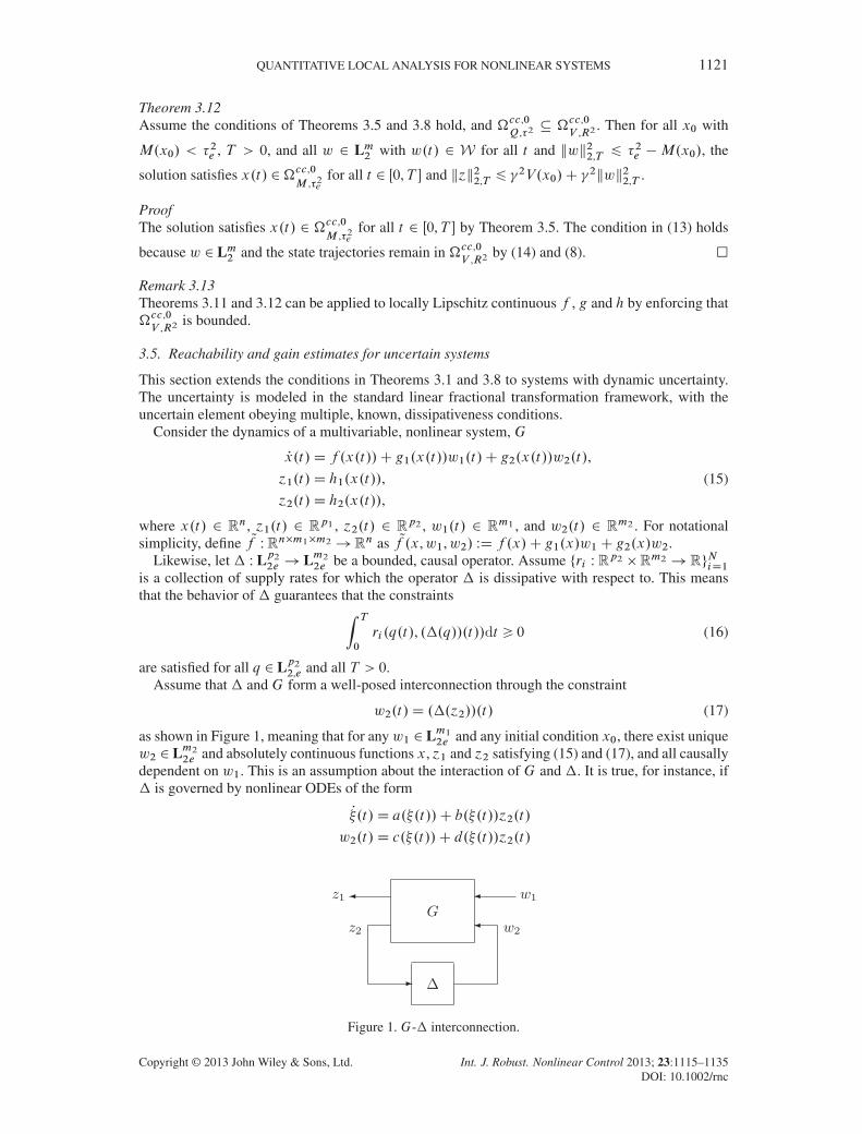
w2.t/D .�.´2//.t/ (17)
as shown in Figure 1, meaning that for anyw1 2 Lm12e and any initial condition x0, there exist uniquew2 2 Lm22e and absolutely continuous functions x, ´1 and ´2 satisfying (15) and (17), and all causallydependent on w1. This is an assumption about the interaction of G and �. It is true, for instance, if� is governed by nonlinear ODEs of the form
P�.t/D a.�.t//C b.�.t//´2.t/
w2.t/D c.�.t//C d.�.t//´2.t/
Figure 1. G-� interconnection.
Copyright © 2013 John Wiley & Sons, Ltd. Int. J. Robust. Nonlinear Control 2013; 23:1115–1135DOI: 10.1002/rnc

1122 E. SUMMERS ET AL.
for Lipschitz continuous functions a, b, c and d .The following proposition analyzes the interconnection, establishing L2 gain bounds from w1 to
´1 valid for all operators � that are dissipative with respect to the supply rates r1, : : : , rN .
Theorem 3.14Suppose W1 � Rm1 . Assume that f , g1, g2, h1, and h2 in (15) are Lipschitz continuous. Letr1, : : : , rN WRp2�m2 !R. Suppose there exist constant � > 0,R > 0, nonnegative �i 2 R, ˇi 2R,differentiable functions Q WRn!R and V WRn!R that satisfy Q.0/D V.0/D 0,
�cc,0Q,�2��cc,0
V ,R2(18)
�cc,0V ,R2n 0� ¹x 2Rn W V.x/ > 0º (19)
�cc,0Q,�2�
´x 2Rn W rQ.x/ � Qf .x,w1,w2/
6 wT1 w1 �NXiD1
�iri .h2.x/,w2/, 8.w1,w2/ 2W1 �Rm2
μ(20)
�cc,0V ,R2�
´x 2Rn W rV.x/ � Qf .x,w1,w2/
6 wT1 w1 �1
2hT1 .x/h1.x/�
NXiD1
ˇiri .h2.x/,w2/, 8.w1,w2/ 2W1 �Rm2
μ. (21)
Consider x0 2 �cc,0Q,�2
with Q.x0/ < �2, T > 0, and w1 2 Lm12 with w1.t/ 2 W1 for all t . If
kw1k22,T < �2 �Q.x0/, then for all � dissipative with respect to the supply rates r1, : : : , rN , the
solution to (15)–(17) with x.0/D x0 satisfies Q.x.t// < �2 for all t 2 Œ0,T �, and
k´1k22,T 6 2V.x0/C 2kw1k22,T . (22)
ProofSuppose there is a finite T > 0 such that Q.x.T // D �2 and Q.x.t// < �2 for all 0 6 t < T .Hence, x.t/ 2�cc,0
Q,�2for all t 6 T . Integrate PQ from 0 to T , using that x.t/ 2�cc,0
Q,�2, and �cc,0
Q,�2is
contained in the region where the dissipation inequality in (20) holds. This yields
Q.x.T //�Q.x0/6 kw1k22,T �XN
iD1
Z T
0
�iri .h2.x.t/,w2.t/// dt
6 kw1k22,T .
But Q.x.T // D �2, therefore kw1k22,T > �2 � Q.x0/, and the first claim is established. Recall
�cc,0Q,�2��cc,0
V ,R2, so the solutions remain in �cc,0
V ,R2as well. Integrating PV gives
V.x.T //� V.x0/6 kw1k22,T �1
2k´1k
22,T �
XN
iD1
Z T
0
ˇiri .h2.x.t/,w2.t/// dt
6 kw1k22,T �1
2k´1k
22,T .
Because V > 0 on �cc,0V ,R2
, V.x.T //> 0, and therefore, k´1k22,T 6 2V.x0/C 2kw1k22,T . �
Copyright © 2013 John Wiley & Sons, Ltd. Int. J. Robust. Nonlinear Control 2013; 23:1115–1135DOI: 10.1002/rnc
QUANTITATIVE LOCAL ANALYSIS FOR NONLINEAR SYSTEMS 1123
Remark 3.15In a manner analogous to Theorem 3.4 and Corollary 3.10, results for locally Lipschitz f , g1, g2,h1 and h2 can be derived. Assume conditions (18)–(21) hold, and in addition, �cc,0
Q,�2is bounded.
Use Lemma 8.1 to define globally Lipschitz functions Qf , Qgi and Qhi , which equal, respectively, f ,giand hi on�cc,0
Q,�2. Following (15), define a multivariable system QG using these functions. If� and QG
form a well-posed interconnection and� is dissipative with respect to ¹riºNiD1, then the conclusionsof Theorem 3.14, still regarding the behavior of the interconnection of � and G, remain true.
4. APPLICATION TO A LOCALLY STABLE SCALAR SYSTEM
In this section, we calculate, analytically, the performance characterizations from Section 3,focusing on a one-state, not-uncertain system, to maintain simplicity in the example.
4.1. Reachability calculations
Beacuse (1) restricts the vector fields .f .x/Cg.x/w/ to be affine in w, the maximizing w 2Rn DWW in (3) is 1
2gT .x/rQT .x/. Plugging this in and setting the maximum to be zero (the limit for (3)
to be satisfied) gives a quadratic equality in rQ.x/. Considering scalar systems (n D m D 1),
notateQ0.x/ WD rQ.x/, and we obtain 14g2.x/Q02.x/CQ0.x/f .x/D 0. Hence,Q0.x/D�4f .x/
g2.x/
and
Q.x/D
Z x
0
�4f .�/
g2.�/d� . (23)
If g.x/ ¤ 0 for all x, then Q.x/ is well defined for all x and Q0.x/Œf .x/C g.x/w� 6 w2 holdsfor all x 2 R and for all w 2 R. Thus, (2) holds for any � > 0. For such � , if f and g areLipschitz continuous, then the conditions of Theorem 3.1 are satisfied. If f and g are locallyLipschitz continuous and �cc,0
Q,�2is bounded, then the conditions of Theorem 3.4 are satisfied.
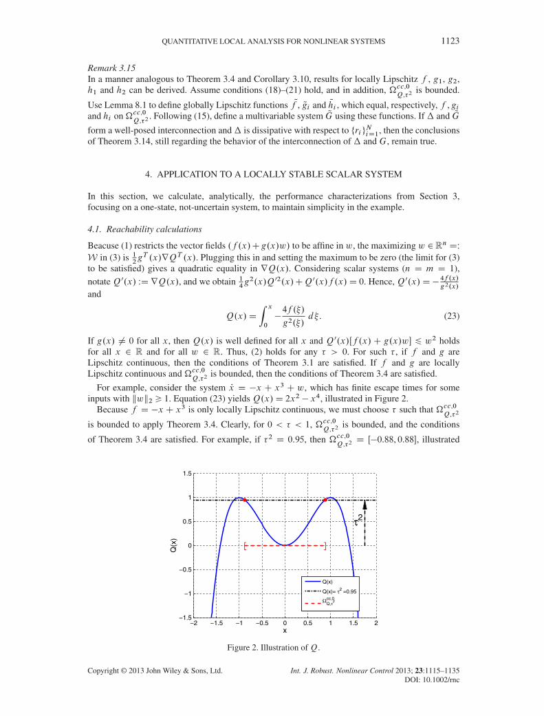
For example, consider the system Px D �x C x3 C w, which has finite escape times for someinputs with kwk2 > 1. Equation (23) yields Q.x/D 2x2 � x4, illustrated in Figure 2.
Because f D �x C x3 is only locally Lipschitz continuous, we must choose � such that �cc,0Q,�2
is bounded to apply Theorem 3.4. Clearly, for 0 < � < 1, �cc,0Q,�2
is bounded, and the conditions
of Theorem 3.4 are satisfied. For example, if �2 D 0.95, then �cc,0Q,�2
D Œ�0.88, 0.88�, illustrated
−2 −1.5 −1 −0.5 0 0.5 1 1.5 2−1.5
−1
−0.5
0
0.5
1
1.5
τ2
[ ]
x
Q(x
)
Q(x)
Q(x)= τ2 =0.95
Ωcc,0Q,τ2
Figure 2. Illustration of Q.
Copyright © 2013 John Wiley & Sons, Ltd. Int. J. Robust. Nonlinear Control 2013; 23:1115–1135DOI: 10.1002/rnc
1124 E. SUMMERS ET AL.
in Figure 2. Thus, for all jx0j < 0.88 and w 2 L2 with kwk2 < 0.95 �Q.x0/, solutions satisfyjx.t/j6 0.88 for all t .
4.2. L2-Gain calculations
Analogous to reachability, the maximizing w in the DIE (11) is 12gT .x/rV T .x/, and setting the
maximum to zero yields a quadratic inequality in rV.x/. Again, we solve this for a scalar system.At the maximizing w with zero as the maximum, we obtain
1
4g2.x/V 02.x/C V 0.x/f .x/C
1
2h2.x/D 0. (24)
Applying the quadratic formula to (24) yields
V 0.x/D
8̂̂<ˆ̂:
2��f .x/�
qf 2.x/� 1
�2g2.x/h2.x/
�g2.x/
for x < 0
2��f .x/C
qf 2.x/� 1
�2g2.x/h2.x/
�g2.x/
for x > 0.
Setting V.0/ D 0 gives V.x/ DZ x
0
V 0.�/ d� . Assume g.x/ ¤ 0 for all x 2 R. Note that V 0.x/ is
real for all x such that f 2.x/� 1�2g2.x/h2.x/> 0. Let R be such that �cc,0
V ,R2n 0� ¹x W V.x/ > 0º.
The inequality
V 0.x/Œf .x/C g.x/w�6 w2 � 1
2h2.x/ (25)
holds for all x 2 �cc,0V ,R2
and for all w 2 R. If f , g, and h are Lipschitz continuous and V.0/ D 0,then the assumptions of Theorem 3.8 are satisfied. If f , g and h are locally Lipschitz continuous,V.0/D 0, and �cc,0
V ,R2is bounded, then the assumptions of Corollary 3.10 are satisfied.
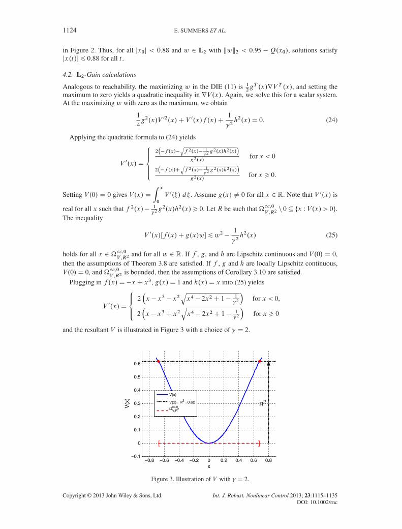
Plugging in f .x/D�xC x3, g.x/D 1 and h.x/D x into (25) yields
V 0.x/D
8̂<:̂2�x � x3 � x2
qx4 � 2x2C 1� 1
�2
�for x < 0,
2�x � x3C x2
qx4 � 2x2C 1� 1
�2
�for x > 0
and the resultant V is illustrated in Figure 3 with a choice of D 2.
−0.8 −0.6 −0.4 −0.2 0 0.2 0.4 0.6 0.8−0.1
0
0.1
0.2
0.3
0.4
0.5
0.6
][
R2
x
V(x
)
V(x)
V(x)= R2 =0.62
Ωcc,0V,R
2
Figure 3. Illustration of V with D 2.
Copyright © 2013 John Wiley & Sons, Ltd. Int. J. Robust. Nonlinear Control 2013; 23:1115–1135DOI: 10.1002/rnc

QUANTITATIVE LOCAL ANALYSIS FOR NONLINEAR SYSTEMS 1125
Let ˛ Dq��1�
and note that V.x/ is real for all x such that jxj 6 ˛. Thus, for any R2 < V.˛/,
�cc,0V ,R2
is bounded and �cc,0V ,R2
n 0 � ¹x W V.x/ > 0º, satisfying Corollary 3.10. For example, let
D 2 (V as in Figure 3) and R2 D 0.62, then �cc,0V ,R2
D Œ�0.68, 0.68�. Thus, by Corollary 3.10, thesolution satisfies jx.t/j< 0.68 and
kyk2,T 6 2pV.x0/C 2kwk2,T
for all jx0j< 0.68, T > 0, and all w 2 L2 with kwk22,T 6 0.62� V.x0/.We can further improve the bound on the gain by exploiting the reachability argument. From
Theorem 3.11, given > 0, we restrict �cc,0Q,�2� �cc,0
V ,R2. In the case of D 2 and R2 D 0.62, we
simply equate �cc,0Q,�2D �cc,0
V ,0.62 D Œ�0.68, 0.68�, which results in �2 D 0.711. Thus, the bound on
kwk2 is increased from kwk22,T 6 0.62 � V.x0/ to kwk22,T 6 0.711 �Q.x0/, whereas the boundon the gain remains D 2. The increase is shown in Figure 4. We repeat this procedure for arange of values to obtain a curve, shown in Figure 5, of the gain based on the size of the inputassuming x0 D 0. Note that the bound on the input approaches 1 as the gain increases, which is
−0.8 −0.6 −0.4 −0.2 0 0.2 0.4 0.6 0.8−0.1
0
0.1
0.2
0.3
0.4
0.5
0.6
0.7
0.8
x0
22
0.62−V(x0)
0.711−Q(x0)
Figure 4. The bound on the input is shown as a function of the initial condition x0. After applyingTheorem 3.11, the input bound is increased for all x0 2 Œ�0.68, 0.68�.
0.1 0.2 0.3 0.4 0.5 0.6 0.7 0.8 0.9 11
2
3
4
5
6
7
8
2, T
L2 Gain BoundImprovement after Reachability
Figure 5. The L2 gain bound is improved after applying Theorem 3.11.
Copyright © 2013 John Wiley & Sons, Ltd. Int. J. Robust. Nonlinear Control 2013; 23:1115–1135DOI: 10.1002/rnc

1126 E. SUMMERS ET AL.
expected because the dynamical system under consideration has finite escape times for some inputskwk2,T > 1.
5. PERFORMANCE CHARACTERIZATIONS AS SUM-OF-SQUARES CONDITIONS
In this section, we outline the computational methods used to verify the conditions in Section 3 usingSOS programming [39, 51, 52], introduced in the Appendix. Assume f , g, and h in (1) are polyno-mials and are therefore locally Lipschitz continuous. The Q and V in Theorem 3.4, Corollary 3.10and Remark 3.13 will also be restricted to be polynomial. The S-procedure, in the Appendix, givesa sufficient condition to verify containments of sets described by inequalities.
5.1. Reachability, refinement and L2-gain formulations
The results of Theorems 3.1, 3.5 and 3.4 show that a partial DIE yields an outer bound on statesreachable from a given initial condition, driven by a ball of L2 disturbances. For various sets ofdisturbances, the exact reachable set can be described in terms of a sublevel set of a generalizedstorage function that satisfies a PDE [27]. The numerical methods outlined in this section search forstorage functions from a limited class (e.g., polynomial of degree 4). Generally, this class will notinclude the ‘real’ storage function, and as a consequence, the PDE has been relaxed, for example,into the inequality presented in theorems, to admit meaningful solutions from a prespecified func-tion class. The relaxed partial differential inequalities, by their nature, have many solutions. Amongall solutions, the techniques presented are geared toward solutions, which improve the reachabilitybound relative to a particular shape the analyst proposes. The analyst can specify a set P for whichthe goal is to show that all states reachable from x.0/D 0 and kwk22 < �
2 are contained in P . Aug-menting the conditions of Theorems 3.1 and 3.4 (and corollaries) with the requirement �Q,�2 � Pensures the containment. More flexible is to use an adjustable region derived from a given functionp WRn!R, called the shape-factor function, defining P WD�p,ˇ . The function p is usually simple(e.g., quadratic), so that even in high dimensions, its sublevel sets are easily interpreted (in contrastto Q, whose sublevel sets may be difficult to quantify). Much like a weight parameter as part of acost function in optimal control, the positive-definite function p is chosen by the analyst to reflectthe relative importance of the individual state elements. Hence, assume a shape-factor function p,with bounded sublevel sets, is given. The condition�cc,0
Q,�2��p,ˇ is enforced with the S-procedure,
which actually certifies more, namely �Q,�2 � �p,ˇ . The set W is defined in terms of a sublevelset of a polynomial function pW , with W WD ¹w W pW .w/> 0º.
Translating the results of 3.1 (and 3.4) into SOS conditions employs two applications of theS-procedure: one for �Q,�2 � �p,ˇ in Rn and one for DIE containment of (3), in Rn � Rm. Forgiven � > 0, the conditions
s1 2†nCm, s2 2†n, sp 2†nCm, Q 2†n, Q.0/D 0 (26)
wTw �rQ � .f C gw/� s1 � .�2 �Q/� sppW 2†nCm, (27)
ˇ � p � s2 � .�2 �Q/ 2†n (28)
guarantee the hypothesis of Theorem 3.4 and �Q,�2 ��p,ˇ .Implementation of Theorem 3.5 is relatively simple because a storage function Q and constant
� that satisfy Theorem 3.4 are given. The computational objective is to find a suitable functionk W Œ0 �2� ! R satisfying (6). The simplest approach restricts k to be piecewise constant. Forexample, take N > 0, and let ¹kiºNiD1 denote the function values, with k given by nearest neighbor
interpolation, defining WD �2
Nand k.�/D ki for all .i �1/6 � < i for i D 1, : : : ,N . Employing
the S-procedure, obtaining optimal values for the ¹kiºNiD1, only requires N uncoupled, linear SOSoptimizations, namely for i D 1, : : : ,N
Copyright © 2013 John Wiley & Sons, Ltd. Int. J. Robust. Nonlinear Control 2013; 23:1115–1135DOI: 10.1002/rnc

QUANTITATIVE LOCAL ANALYSIS FOR NONLINEAR SYSTEMS 1127
minimizes1i ,s2i ,spi
ki
subject to s1i 2†nCm, s2i 2†nCm, spi 2†nCm,
� Œ. i �Q/s1i C .Q� .i � 1//s2i CrQ.f C gw/� kiwTw�� spipW 2†nCm.
Using the resultant piecewise constant k yields �2e DZ �2
0
k�1.�/d� D
NXiD1
k�1i .
For L2 gain, only one application of the S-procedure is used for the DIE containment of (11) inRn �Rm, which requires the SOS polynomial to be in †nCm. If V is restricted to be a polynomial,then for given > 0 and R > 0, and polynomial l.x/ > 0 for all x ¤ 0, l.0/ D 0, the conditionsV.0/D 0,
s3 2†nCm, sp 2†nCm, (29)
V � l 2†n, (30)
wTw �1
2h.x/T h.x/�rV � .f .x/C g.x/w/� s3.R
2 � V /� sppW 2†nCm (31)
satisfy the conditions of Corollary 3.10. Note that (31) actually implies the DIE holds on �V ,R2 ,not just the connected component, as in (11). Following Theorem 3.11, the reachability equations,(26)–(28), can be solved (maximizing � ) with p WD V and ˇ WD R2. It is straightforward to showthat any V and R in (29)–(31), � WDR and Q WD V are feasible for (26)–(28).
The corresponding robust versions, for use with Theorem 3.14, simply include the supply rates ofthe known dissipativeness conditions and account for the signals w1,w2, ´1 and ´2. For example,condition (21) is ensured by a generalization to (31),
wT1 w1�1
2hT1 h1�rV �.f Cg1w1Cg2w2/�s3.R
2�V /�sppW �
nXiD1
ˇiri .h2,w2/ 2†nCm1Cm2
(32)constrained by ˇi > 0, as well as the original constraints on the various SOS multipliers.
5.2. Feasibility guarantee
Many standard results from nonlinear system theory show that properties of the linearized dynami-cal system carry over to local properties of the nonlinear system, for instance, exponential stabilityof an equilibrium point of an autonomous system [53]. In [13], we explored how properties of thelinearized system implied the corresponding feasibility of the SOS formulations (Section 5), usingquadratic storage functions, for three types of problems: ROA, reachability and L2 gain. In [13],the vector field was limited to cubic polynomials, and the proof techniques geared toward systemsof that class. In this section, we extend these results to polynomial vector fields of any degree. Forbrevity, we only consider L2 gain formulation (section 3.3) although the other results follow as well,including the uncertain L2 gain formulation from Section 3.5.
The results here are similar in spirit, although different and of significantly weaker theoreticalvalue, to other results in the literature. The work of Peet [20] establishes the optimality of polynomialstorage functions for certain stability questions, using Positivestellensatz-based proofs (generaliza-tion of the simple S-procedure). By contrast, the results in [22] are negative, showing the inadequacyof polynomial storage functions in answering stability questions for a special class of nonlinearautonomous systems.
A simple technical lemma (proof in Appendix) is used in the subsequent claim.
Lemma 5.1Let d > 2 be a positive integer. Let V.x/ WD xTQx with 0 � Q D QT 2 Rn�n. Let r.x/ denotethe vector of all monomials of degree 1 through degree d � 1 and s.x/D r.x/T r.x/. Similarly, let´.x/ denote the vector of all monomials of degree 2 through degree d . The length of ´ is denotedn´. There exists H 2 Rn´�n´ with H DHT � 0 and s.x/V .x/D ´.x/TH´.x/.
Copyright © 2013 John Wiley & Sons, Ltd. Int. J. Robust. Nonlinear Control 2013; 23:1115–1135DOI: 10.1002/rnc

1128 E. SUMMERS ET AL.
Now, write the affine-in-w system in (1) as
Px.t/D Ax.t/CBw.t/C f2.x.t//C g1.x.t//w.t/
y.t/D Cx.t/C h2.x.t//(33)
where f2,g1 and h2 are polynomials, respectively, consisting of terms of degrees 2, 1, and 2 (andhigher). Let @.f2/, @.h2/ and @.g1/ denote the highest degree of monomials within each function.Define d WDmax¹@.f2/, @.h2/, @.g1/C 1º. Suppose the linearization has A Hurwitz, and for some > 0,
��C.sI �A/�1B��1< . By the bounded-real lemma, there exists P D P T � 0 such that"
ATP CPAC 1�2C TC PB
BTP �I
#� 0.
Defining V.x/ WD xTPx and s WD ˛rT .x/r.x/ leads to the main SOS constraint as
2xTP ŒAxCBwC f2.x/C g1.x/w��wTw
C1
2
�xTC T C hT2 .x/
�ŒCxC h2.x/�C ˛
�R2 � xTPx
�rT .x/r.x/.
This is a quadratic form in ŒxIwI ´.x/� as follows. There exist matrices F and H such thatf2.x/ D F´.x/ and h2.x/ D H´.x/. Likewise, there exists a matrix G such that xTPg1.x/w DwTG´.x/. By Lemma 5.1, there exists a positive-definite matrixMP such that rT .x/r.x/xTPx D´T .x/MP´.x/. Finally, there exists a matrix E such that rT .x/r.x/D xT xC´.x/TE´.x/. Whencombined, we have the expression
24 x
w
´.x/
35T
2664ATP CPAC 1
�2C TC C ˛R2I PB PF C 1
�C TH
BTP �I G
F TP C 1�HC GT ˛R2E C 1
�2HTH � ˛MP
3775
„ ƒ‚ …K.R,˛/
24 x
w
´.x/
35
At R WD 0, the top/left 2� 2 block is negative definite, and MP � 0. Hence, for sufficiently large ˛,it follows that K.0,˛/ � 0. With such an ˛ chosen, by continuity, there exists nonzero R such thatK.R,˛/� 0. The previous reasoning is summarized in a theorem.
Theorem 5.2Assume x D 0 is an equilibrium of (1) and express the vector field with linear and nonlinear termsseparated, as in (33). If A is Hurwitz, and
��C.sI �A/�1B��1< , then there exist R > 0, > 0,
quadratic V and polynomial s3 (with sp D 0) such that (29)–(31) are feasible using l.x/ WD xT x.
5.3. Iteration Strategy
Equations (26)–(28) and (29)–(31) constitute a nonconvex optimization problem, namely a linearobjective subject to bilinear matrix inequality constraints. Acknowledging the theoretical implica-tions [54, 55], we nevertheless push forward with iterative schemes to generate feasible solutions,and further optimize the cost. We outline an iteration for (29)–(31). Analogous iterations are possiblefor (26)–(28) by replacing V with Q, R with � , and s3 with s1, s2.
1. On the basis of the polynomials f , g and h (and their degrees), choose basis functions for theunknowns sp , s3 and V . At present, computational restrictions (memory, numerical condition-ing, algorithms etc.) place a practical restriction on the overall degree of the DIE polynomialin terms of the number of independent variables (nCm), which in turn, limits the degrees ofsp , s3 and V .
2. If the linearization is stable, then use the LMI derived in Section 5.2 to obtain feasible valuesfor s3 and V (using sp D 0). If the linearization is not stable, then the DIE is relaxed and the
Copyright © 2013 John Wiley & Sons, Ltd. Int. J. Robust. Nonlinear Control 2013; 23:1115–1135DOI: 10.1002/rnc

QUANTITATIVE LOCAL ANALYSIS FOR NONLINEAR SYSTEMS 1129
constraint violation is minimized. If this minimum is less than 0, then feasible values for Vand s3 for the original problem are obtained.
3. [R Maximization]: Hold V fixed, and maximize R, by choice of s3 and sp such that (29) and(31) hold. This step requires a bisection in R, where for each fixed value of R, determiningfeasible s3, sp is a linear SOS problem.
4. [V Recenter]: Hold s3 fixed, and ‘recenter’ V by finding the analytic center (inR2, parametersof sp , parameters of V , and parameters associated with the kernel representation of the SOSproblem [52]) of system of LMI constraints defined by (30) and (31).
5. Return to the [R Maximization] step, and repeat.
6. EXAMPLES
In the following examples, we utilize the SOS optimization tool SOSOPT and associated nonlinearsystems analysis software, available at http://www.aem.umn.edu/AerospaceControl/.Supporting material, documentation, and additional examples can be found in [56].
6.1. Scalar example from Section 4
We revisit the example in Section 4 and compare those results with the SOS-based iteration fromSection 5.3. Using quadratic V and Q, we compared the results in Figure 6. The V obtained fromthe L2 analysis is used as the shape-factor function in the reachability analysis, which improves thebound and then improved further with refinement. A power algorithm from [57] attempts to findinput signals, of a given norm, which maximize the resultant output norm, yielding a lower boundon the system L2 gain (also shown).
6.2. Three-state reach example
Consider the three state system, extending an example in [58]: Px1 D�x3Cx2�x3x22 I Px2 D�x2x23�
x2CwI Px3 D12.x1 � x3/. For purposes of illustration, choose p.x/ WD 8x21 � 8x1x2C 4x
22 C x
23 .
Given ˇ > 0 and a basis for Q, we maximize � such that the conditions of Theorem 3.1 hold and�Q,�2 � �p,ˇ , which will further imply that Theorem 3.4 holds because �Q,�2 is bounded. Weperform the analysis for ˇ 2 .0, 50/ using both quadratic and quartic Q. In both cases, the SOSmultipliers s1 and s2 are chosen constant and quadratic, respectively. Conversely, a power algorithmfrom [57] attempts to find inputs on a finite horizon, of a given norm, which maximize p.x.Tfinal//.The algorithm is globally convergent for linear systems but can also be applied to nonlinear systemsas an ad hoc manner to find the worst-case input. In that context, the results it produces are lower
0 0.1 0.2 0.3 0.4 0.5 0.6 0.7 0.8 0.9 11
1.5
2
2.5
3
3.5
4
4.5
5
2
Bou
nd o
n G
ain
γ
L2 Gain Using SOS
Reachability Using SOS
Refinement Using SOS
Bound from L2 DIE
Bound from Reachability DIE
Lower Bound
Figure 6. Comparison of the SOS approach with the algebraic approach in Section 4.
Copyright © 2013 John Wiley & Sons, Ltd. Int. J. Robust. Nonlinear Control 2013; 23:1115–1135DOI: 10.1002/rnc
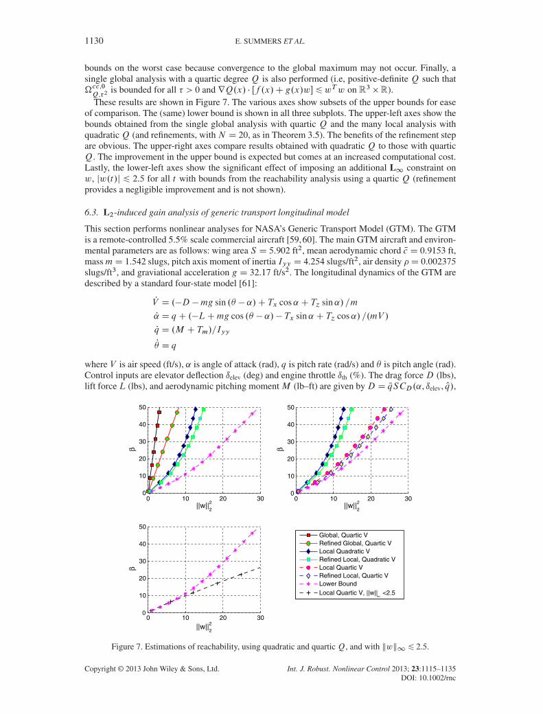
1130 E. SUMMERS ET AL.
bounds on the worst case because convergence to the global maximum may not occur. Finally, asingle global analysis with a quartic degree Q is also performed (i.e, positive-definite Q such that�cc,0Q,�2
is bounded for all � > 0 and rQ.x/ � Œf .x/C g.x/w�6 wTw on R3 �R).These results are shown in Figure 7. The various axes show subsets of the upper bounds for ease
of comparison. The (same) lower bound is shown in all three subplots. The upper-left axes show thebounds obtained from the single global analysis with quartic Q and the many local analysis withquadraticQ (and refinements, with N D 20, as in Theorem 3.5). The benefits of the refinement stepare obvious. The upper-right axes compare results obtained with quadratic Q to those with quarticQ. The improvement in the upper bound is expected but comes at an increased computational cost.Lastly, the lower-left axes show the significant effect of imposing an additional L1 constraint onw, jw.t/j 6 2.5 for all t with bounds from the reachability analysis using a quartic Q (refinementprovides a negligible improvement and is not shown).
6.3. L2-induced gain analysis of generic transport longitudinal model
This section performs nonlinear analyses for NASA’s Generic Transport Model (GTM). The GTMis a remote-controlled 5.5% scale commercial aircraft [59,60]. The main GTM aircraft and environ-mental parameters are as follows: wing area S D 5.902 ft2, mean aerodynamic chord Nc D 0.9153 ft,massmD 1.542 slugs, pitch axis moment of inertia Iyy D 4.254 slugs/ft2, air density �D 0.002375slugs/ft3, and graviational acceleration g D 32.17 ft/s2. The longitudinal dynamics of the GTM aredescribed by a standard four-state model [61]:
PV D .�D �mg sin .� � ˛/C Tx cos˛C T´ sin˛/ =m
P̨ D qC .�LCmg cos .� � ˛/� Tx sin˛C T´ cos˛/ =.mV /
Pq D .M C Tm/=Iyy
P� D q
where V is air speed (ft/s), ˛ is angle of attack (rad), q is pitch rate (rad/s) and � is pitch angle (rad).Control inputs are elevator deflection ıelev (deg) and engine throttle ıth (%). The drag force D (lbs),lift force L (lbs), and aerodynamic pitching momentM (lb–ft) are given byD D NqSCD.˛, ıelev, Oq/,
0 10 20 300
10
20
30
40
50
2
2
2
2
2
2
β
0 10 20 300
10
20
30
40
50
β
0 10 20 300
10
20
30
40
50
β
Global, Quartic VRefined Global, Quartic VLocal Quadratic VRefined Local, Quadratic VLocal Quartic VRefined Local, Quartic VLower Bound
∞ <2.5
Figure 7. Estimations of reachability, using quadratic and quartic Q, and with kwk1 6 2.5.
Copyright © 2013 John Wiley & Sons, Ltd. Int. J. Robust. Nonlinear Control 2013; 23:1115–1135DOI: 10.1002/rnc

QUANTITATIVE LOCAL ANALYSIS FOR NONLINEAR SYSTEMS 1131
L D NqSCL.˛, ıelev, Oq/ and M D NqS NcCm.˛, ıelev, Oq/, where Nq WD 12�V 2 is the dynamic pressure
(lbs/ft2) and Oq WD Nc2Vq is the normalized pitch rate (unitless). CD , CL, and Cm are unitless aero-
dynamic coefficient functions provided as look-up tables by NASA. The GTM has one engine onthe port side and one on the starboard side of the airframe. The thrust from a single engine T (lbs)is a function of the throttle setting ıth (percent). T .ıth/ is specified as a ninth-order polynomial inNASA’s high fidelity GTM simulation model. Tx (lbs) and T´ (lbs) denote the projection of the totalengine thrust along the body x-axis and body z- axis, respectively. Tm (lbs–ft) denotes the pitchingmoment due to both engines.
The following terms of the longitudinal model are approximated by low-order polynomials:Trigonometric functions; engine model; rational dependence on speed (1=V ); and aerodynamiccoefficients (CD , CL, Cm). The trigonometric functions are approximated by Taylor series expan-sions. For the engine model, least squares is used to approximate the ninth-order polynomialfunction T .ıth/ by a third-order polynomial. Least squares is also used to compute a linear fit to1/V over the desired range of interest from 100 ft/s to 200 ft/s. Finally, polynomial least squaresfits are computed for the aerodynamic coefficient look-up tables provided by NASA. A degree 7polynomial model, provided in [46], is obtained after replacing all nonpolynomial terms with theirpolynomial approximations.
The polynomial model takes the form Px D f7.x,u/ where x WD ŒV (ft/s), ˛(rad), q (rad/s),� (rad)�T , and u WD Œıelev(deg), ıth.%/�T . The subscript in f7 denotes that the vector field is adegree 7 polynomial in x. The quality of the polynomial approximation was assessed by comparingthe trim conditions and simulation responses of the polynomial and original nonpolynomial mod-els. The following straight and level flight condition was computed for this model: Vt D 150 ft/s,˛t D 0.047 rad, qt D 0 rad/s, �t D 0.047 rad, with ıelev,t D 0.051 rad, ıth,t D 14.78%. The subscriptt denotes a trim (equilibrium) value. A cubic-order polynomial longitudinal model is extracted fromthe four-state, degree 7 polynomial model by holding ıth at its trim value and retaining terms up tocubic order. The cubic-order model is Px D f3.x,u/ with four states ŒV , ˛, q, and ��T and oneinput u WD ıelev. This cubic model is used for all analyses described in the remainder of the section.Additional details on the polynomial modeling are provided in [46], and files containing the modelcan be found at [56].
An L2! L2 gain analysis was first performed on the open-loop model by injecting a disturbancew at the elevator input. Figure 8 indicates how the induced gain of this open-loop system varies as
0 0.02 0.04 0.0610
20
30
40
50
60
2
Indu
ced
Gai
n,
γ
L2 Gain: OL QuadraticL2 Gain: OL QuarticL2 Gain: CL QuadraticReach: CL QuadraticRefine: CL QuadraticL2 Gain: CL QuarticReach: CL QuarticRefine: CL Quartic
Figure 8. Upper bounds of L2! L2 gain from w to q for open and closed-loop GTM model.
Copyright © 2013 John Wiley & Sons, Ltd. Int. J. Robust. Nonlinear Control 2013; 23:1115–1135DOI: 10.1002/rnc
1132 E. SUMMERS ET AL.
the size of the elevator disturbances jjwjj2 increases. The horizontal axis indicates the size of theelevator disturbances, jjwjj2, around the trim input value, and the vertical axis shows the boundsof the induced gain from disturbance w to pitch rate q. The bounds are calculates for several fixedvalues of by maximizingR over the choice of V and s3 such that (29)–(31) hold using the strategyfrom Section 5.3. Figure 8 shows the open-loop results for both a quadratic (black dashed-’}’) and aquartic (black solid-’}’) storage function V . The higher (quartic)-degree storage function providesa less conservative bound on the gain, as expected. The induced gain for the linearized open-loopsystem is 23.9. Both nonlinear bounds converge to this linearized gain as kwk2! 0.
The open-loop dynamics of the GTM are slightly underdamped. Inner loop pitch rate feedbackis typically used to improve the damping of the aircraft. A proportional pitch rate feedback isused to improve the damping of the GTM aircraft. Combining with the input disturbance givesıelev DKqqCw D 0.0698qCw where w is the input disturbance at the elevator channel. Figure 8also shows bounds on the closed-loop L2 gain from elevator disturbances to pitch rate for a quadratic(red dashed-’x’) and a quartic ( blue solid-’x’) storage function V . Again, the higher (quartic)-degreestorage function provides a less conservative bound on the gain. Moreover, the pitch-rate dampinglowers the induced gain for the linearized closed-loop system to 16.6. Both nonlinear bounds forthe closed-loop system converge to this linearized gain as kwk2! 0. Finally, as expected, the gainbounds for the closed-loop system are both below the open-loop bounds.
The refinement procedures were used to improve the computed bounds for the closed-loop sys-tem. First, the reachability analysis is performed by setting V as the shape-factor function andmaximizing � over choice of Q, s1 and s2 such that (26)–(28) hold. Figure 8 shows the resultsobtained when the degree of Q is restricted to be quadratic (red dashed-’o’) and quartic (bluesolid-’o’). Finally, the refinement is performed on the quadratic (red dashed-’+’) and quartic (bluesolid-’+’) results from the reachability. These results show that the bound on the allowable inputis improved from the reachability analysis and improved further by the refinement procedure.As expected, the upper bounds on the gain using quartic V and Q are improvements over theirquadratic counterparts.
APPENDIX A: LIPSCHITZ EXTENSIONS
Locally Lipschitz continuous functions can be extended to globally Lipschitz continuous functionsas follows [62, 63].
Lemma 8.1Let f W Rn ! R be Lipschitz continuous on B � Rn with B ¤ ; and Lipschitz constant L. Foreach x 2Rn, define Qf WRn!R
Qf .x/ WDminy2B
f .y/CL kx � yk . (34)
Then Qf .x/D f .x/ 8x 2 B and Qf is globally Lipschitz continuous (with Lipschitz constant L).
ProofConsider first the case x 2 B. Clearly, Qf .x/ 6 f .x/ because Qf involves a minimum over all y 2 Band the value obtained at y D x 2 B is f .x/. Next, because f is Lipschitz continuous on B, itfollows that f .x/ 6 f .y/C L kx � yk for all y 2 B. Minimizing the right-hand side over y 2 B(which gives Qf .x/) preserves the inequality; hence, f .x/ 6 Qf .x/. Together these imply that forx 2 B, Qf .x/D f .x/.
For global Lipschitz continuity of Qf , take any x1 2Rn, x2 2Rn. For all ´ 2Rn,
f .´/CL kx1 � ´k6 f .´/CL kx2 � ´kCL kx1 � x2k .
Minimize both sides of this expression over ´ 2 B to get Qf .x1/ 6 Qf .x2/ C L kx1 � x2k.Reversing the role of x1 and x2 gives Qf .x2/ 6 Qf .x1/ C L kx2 � x1k. Combining these givesˇ̌̌Qf .x1/� Qf .x2/
ˇ̌̌6 L kx1 � x2k as desired. �
Copyright © 2013 John Wiley & Sons, Ltd. Int. J. Robust. Nonlinear Control 2013; 23:1115–1135DOI: 10.1002/rnc

QUANTITATIVE LOCAL ANALYSIS FOR NONLINEAR SYSTEMS 1133
APPENDIX B: POLYNOMIALS, SUM-OF-SQUARES AND S-PROCEDURE
A monomial m˛ in n variables is a function defined as m˛.x/D x˛ WD x˛11 x
˛22 � � � x
˛nn for ˛ 2 ZnC.
The degree of a monomial is defined, degm˛ WDPniD1 ˛i . A polynomial f in n variables is a finite
linear combination of monomials, with c˛ 2R:
f WDX˛
c˛m˛ DX˛
c˛x˛
The set of all polynomials in n indeterminate variables is denoted Rn. The particular variables arenot noted, and usually, there is an obvious n-dimensional variable present in the discussion. Thedegree of f is defined as degf WDmax˛ degm˛ (provided the associated c˛ is nonzero).
The notation †n denotes the set of SOS polynomials in n variables,
†n WD
´p 2Rn W p D
tXiD1
f 2i , t > 0,fi 2Rn, i D 1, : : : , t
μ.
If p 2 †n, then p.x/ > 0 8x 2 Rn. The notation †nCm also appears, referring to SOS polyno-mials in nCm real variables, where, again, the particular variables are clear in the context of thediscussion. The following lemma is a trivial generalization of the well-known S-procedure [19] andis a special case of the Positivstellensatz Theorem [64, Theorem 4.2.2].
Lemma 8.2 (Generalized S-procedure)Given ¹piºmiD0 2Rn. If there exist ¹skºmiD1 2†n such that p0 �
PmiD1 sipi 2†n, then
m\iD1
¹x 2Rn W pi .x/> 0º � ¹x 2Rn jp0.x/> 0º.
ProofBecause p0 �
PmiD1 sipi 2 †n, p0 >
PmiD1 sipi 8x. For any Nx 2
TmiD1¹x 2 Rn jpi .x/ > 0º,
because si . Nx/> 0,PmiD1 sipi > 0; hence, p0. Nx/> 0. �
APPENDIX C: PROOF OF LEMMA 5.1
ProofBecause Q � 0, there exists ˛ > 0 such that QQ WD Q � ˛I � 0. Define the perturbed polynomialQV .x/ WD xT QQx. By assumption, s.x/D
Pi ri .x/
2, and hence,
s.x/ QV .x/DXi
ri .x/2xT QQx D
Xi
.ri .x/x/T QQ.ri .x/x/. (35)
Each term in the sum is SOS with positive-definite Gram matrix QQ. Thus, s.x/ QV .x/, being a sumof SOS terms, is itself an SOS polynomial. Because s.x/ QV .x/ contains all monomials of degree 4through degree 2d , it has a Gram matrix decomposition of the form ´.x/T QH´.x/. The existence ofa Gram matrix QH � 0 follows because s.x/ QV .x/ is SOS.
Finally, s.x/V .x/ D s.x/ QV .x/ C ˛Pi ri .x/
2xT x.Pi ri .x/
2xT x is a sum of monomialssquared. The sum includes squares of all monomials in ´.x/ possibly with repeats. Therefore, thissum has a Gram matrix decomposition of the form ´.x/TD´.x/ where D is diagonal and positive-definite. Thus, s.x/V .x/ has a Gram representation ´T .x/H´.x/ where H D QH C ˛D � 0. �
ACKNOWLEDGEMENTS
The authors would like to thank Professor Craig Evans and Dr. Ryan Hynd for several helpful discus-sions. This material is based upon work supported under a National Science Foundation Graduate ResearchFellowship, the NASA Harriet Jenkins Predoctoral Fellowship, the Amelia Earhart Fellowship, the Univer-sity of Minnesota Doctoral Dissertation Fellowship, the Boeing Corporation, the NASA Langley NRA con-tract NNH077ZEA001N entitled ‘Analytical Validation Tools for Safety Critical Systems’ and the AFOSRaward FA9550-12-1-0339 entitled ‘A Merged IQC/SOS Theory for Analysis of Nonlinear Control Systems’.
Copyright © 2013 John Wiley & Sons, Ltd. Int. J. Robust. Nonlinear Control 2013; 23:1115–1135DOI: 10.1002/rnc

1134 E. SUMMERS ET AL.
REFERENCES
1. van der Schaft AJ. L2-gain and Passivity Techniques in Nonlinear Control, (2nd edn). Springer-Verlag: New Yorkand Berlin, 2000.
2. Helton J, James M. Extending H1 Control to Nonlinear Systems: Control of Nonlinear Systems to AchievePerformance Objectives, Frontiers in Applied Mathematics. SIAM: Philadelphia, Pa, 1999.
3. Zames G. On the input–output stability of time-varying nonlinear feedback systems-Parts I and II. IEEE Transactionson Automatic Control 1966; 11:228–238 and 465–476.
4. Willems J. Least squares stationary optimal control and the algebraic Riccati equation. IEEE Transactions onAutomatic Control 1971; 16:621–634.
5. Desoer C, Vidyasagar M. Feedback Systems: Input-Output Properties. Academic Press: New York, NY, 1975.6. Megretski A, Rantzer A. System analysis via integral quadratic constraints. IEEE Transactions on Automatic Control
1997; 42(6):819–830.7. Wen J, Arcak M. A unifying passivity framework for network flow control. IEEE Transactions on Automatic Control
2004; 49(2):162–174.8. Arcak M. Passivity as a design tool for group coordination. IEEE Transactions on Automatic Control 2007;
52(8):1380–1390.9. Tan W, Packard A, Wheeler T. Local gain analysis of nonlinear systems. In Proceedings of the ACC, Minneapolis,
MN, 2006; 92–96.10. Tan W, Packard A. Stability region analysis using sum of squares programming. In Proceedings of the ACC,
Minneapolis, MN, 2006; 2297–2302.11. Topcu U. Quantitative local analysis of nonlinear systems. PhD thesis, University of California at Berkeley, 2008.12. Topcu U, Packard A. Local robust performance analysis for nonlinear dynamical systems. In American Control
Conference, 2009, IEEE, Shanghai, China, 2009; 784–789.13. Topcu U, Packard A. Linearized analysis versus optimization-based nonlinear analysis for nonlinear systems. In
American Control Conference, 2009, IEEE, St. Louis, MO, 2009; 790–795.14. Summers E, Packard A. L2 gain verification for interconnections of locally stable systems using integral quadratic
constraints. In Proceedings of the IEEE Conference Decision and Control, Atlanta, GA, 2010; 1460–1465.15. Willems J. Dissipative dynamical systems part I: general theory. Archive for Rational Mechanics and Analysis 1972;
45(5):321–351.16. Hill D, Moylan P. Dissipative dynamical systems: basic input-output and state properties. Journal of the Franklin
Institute 1980; 309(5):327–357.17. Vinter R. A characterization of the reachable set for nonlinear control systems. SIAM Journal on Control and
Optimization 1980; 18(6):599–610.18. Prajna S. Barrier certificates for nonlinear model validation. Automatica 2006; 42(1):117–126.19. Boyd S, El Ghaoui L, Feron E, Balakrishnan V. Linear Matrix Inequalities in System and Control Theory, vol. 15 of
Studies in Applied Mathematics. SIAM: Philadelphia, Pa, 1994.20. Peet M. Exponentially stable nonlinear systems have polynomial Lyapunov functions on bounded regions.
IEEE Transactions on Automatic Control 2009; 54(5):979–987.21. Ahmadi AA, Krstic M, Parrilo PA. A globally asymptotically stable polynomial vector field with no polynomial
lyapunov function. In Proceedings of the IEEE Conference on Decision and Control, Orlando, FL, 2011; 7579–7580.22. Ahmadi A. On the difficulty of deciding asymptotic stability of cubic homogeneous vector fields. In American
Control Conference, Montreal, Canada, 2012; 3334–3339.23. Ebenbauer C, Allgöwer F. Analysis and design of polynomial control systems using dissipation inequalities and sum
of squares. Computers & Chemical Engineering 2006; 30(10-12):1590–1602.24. Papachristodolou A. Scalable analysis of nonlinear systems using convex optimization. Ph.D. Dissertation,
California Institute of Technology, 2005. (Available at http://thesis.library.caltech.edu/1678/) [Accessed onDecember 16, 2012].
25. Prajna S. Optimization-based methods for nonlinear and hybrid systems verification. Ph.D. Dissertation,California Institute of Technology, 2005. (Available at http://thesis.library.caltech.edu/2155/) [Accessed onDecember 16, 2012].
26. Prajna S, Jadbabaie A. Safety verification of hybrid systems using barrier certificates. In Hybrid Systems: Computa-tion and Control, Alur R, Pappas GJ (eds), vol. 2993 of Lecture Notes in Computer Science. Springer-Verlag: Berlin,Germany, 2004; 477–492.
27. Tomlin C, Mitchell I, Bayen AM, Oishi M. Computational techniques for the verification of hybrid systems.Proceedings of the IEEE 2003; 91(7):986–1001.
28. Mitchell I. The flexible, extensible and efficient toolbox of level set methods. Journal of Scientific Computing 2008;35(2-3):300–329.
29. Coutinho D, Fu M, Trofino A, Danes P. L2-gain analysis and control of uncertain nonlinear systems with boundeddisturbance inputs. International Journal of Robust and Nonlinear Control 2008; 18(1):88–110.
30. Zhang H, Dower P, Kellett C. A bounded real lemma for nonlinear L2-gain. In Proceedings of the IEEE Conferenceon Decision and Control, Atlanta, GA, 2010; 2729–2734.
31. Davison E, Kurak E. A computational method for determining quadratic Lyapunov functions for nonlinear systems.Automatica 1971; 7:627–636.
Copyright © 2013 John Wiley & Sons, Ltd. Int. J. Robust. Nonlinear Control 2013; 23:1115–1135DOI: 10.1002/rnc
QUANTITATIVE LOCAL ANALYSIS FOR NONLINEAR SYSTEMS 1135
32. Genesio R, Tartaglia M, Vicino A. On the estimation of asymptotic stability regions: state of the art and newproposals. IEEE Transactions on Automatic Control 1985; 30(8):747–755.
33. Vannelli A, Vidyasagar M. Maximal Lyapunov functions and domains of attraction for autonomous nonlinearsystems. Automatica 1985; 21(1):69–80.
34. Chiang H, Thorp J. Stability regions of nonlinear dynamical systems: a constructive methodology. IEEE Transactionson Automatic Control 1989; 34(12):1229–1241.
35. Chesi G, Garulli A, Tesi A, Vicino A. LMI-based computation of optimal quadratic lyapunov functions for oddpolynomial systems. International Journal of Robust and Nonlinear Control 2005; 15:35–49.
36. Hachicho O, Tibken B. Estimating domains of attraction of a class of nonlinear dynamical systems with LMI methodsbased on the theory of moments. In Proceedings of the IEEE CDC, Las Vegas, NV, 2002; 3150–3155.
37. Tibken B. Estimation of the domain of attraction for polynomial systems via LMIs. In Proceedings of the IEEE CDC,Sydney, Australia, 2000; 3860–3864.
38. Tibken B, Fan Y. Computing the domain of attraction for polynomial systems via BMI optimization methods.In Proceedings of the ACC, Minneapolis, MN, 2006; 117–122.
39. Parrilo P. Structured semidefinite programs and semialgebraic geometry methods in robustness and optimization.PhD thesis, California Institute of Technology, 2000.
40. Coutinho D, de Souza C, Trofino A. Stability analysis of implicit polynomial systems. IEEE Transactions onAutomatic Control 2009; 54(5):1012–1018.
41. Chesi G. Estimating the domain of attraction via union of continuous families of lyapunov estimates. Systems andControl Letters 2007; 56(4):326–333.
42. Chesi G. Domain of Attraction: Analysis and Control via SOS Programming, No. 415 in Lecture Notes in Controland Information Sciences. Springer: Berlin, Germany, 2011.
43. Chesi G. Estimating the domain of attraction for non-polynomial systems via lmi optimization. Automatica 2009;45(6):1536–1541.
44. Zelentovsky A. Nonquadratic Lyapunov functions for robust stability analysis of linear uncertain systems. IEEETransactions on Automatic Control 1994; 39(1):135–138.
45. Papachristodoulou A, Prajna S. On the construction of Lyapunov functions using the sum of squares decomposition.In Proceedings of the IEEE CDC, Las Vegas, NV, 2002; 3482–3487.
46. Chakraborty A, Seiler P, Balas G. Nonlinear region of attraction analysis for flight control verification and validation.Control Engineering Practice 2011; 19(4):335–345.
47. Tedrake R, Manchester I, Tobenkin M, Roberts J. LQR-trees: feedback motion planning via sum-of-squaresverification. International Journal of Robotics Research 2010; 29(8):1038–1052.
48. Anderson J, Papachristodoulou A. A decomposition technique for nonlinear dynamical system analysis. IEEETransactions on Automatic Control 2012; 57(6):1516–1521.
49. Dullerud G, Paganini F. A Course in Robust Control Theory: A Convex Approach. Springer: New York, NY, 2000.50. Evans L. Partial Differential Equations. American Mathematical Society: USA, 1998.51. Lasserre J. Global optimization with polynomials and the problem of moments. SIAM Journal on Optimization 2001;
11(3):796–817.52. Parrilo P. Semidefinite programming relaxations for semialgebraic problems. Mathematical Programming Series B
2003; 96(2):293–320.53. Khalil H. Nonlinear Systems, Vol. 122. Prentice Hall: New Jersey, 2002.54. Hassibi A, How J, Boyd S. A path-following method for solving BMI problems in control. In Proceedings of the
American Control Conference, IEEE, Vol. 2, San Diego, CA, 1999; 1385–1389.55. Kocvara M, Stingl M. Penbmi users guide, 2005. (Available from: http://www.penopt.com) [Accessed on December
16, 2012].56. Balas G, Packard A, Seiler P, Topcu U. Robustness analysis of nonlinear systems. (Avaiable from: http://www.aem.
umn.edu/~AerospaceControl/) [Accessed on December 16, 2012].57. Tierno J, Murray R, Doyle JC. An efficient algorithm for performance analysis of nonlinear control systems.
In Proceedings of the American Control Conference, Seattle, WA, 1995; 2717–2721.58. Jarvis-Wloszek Z, Feeley R, Tan W, Sun K, Packard A. Some controls applications of sum of squares programming.
In Proceedings of the 42nd IEEE Conference on Decision and Control, Vol. 5, Maui, HI, 2003; 4676–4681.59. Cox D. The GTM DesignSim v0905, 2009.60. Murch A, Foster J. Recent NASA research on aerodynamic modeling of post-stall and spin dynamics of large
transport airplanes. In 45th AIAA Aerospace Sciences Meeting and Exhibit, Reno, Nevada, 2007; AIAA Paper2007-0463.
61. Stevens B, Lewis F. Aircraft Control and Simulaion. John Wiley & Sons: Hoboken, NJ, 1992.62. Kirszbraun M. Über die zusammenziehende und Lipschitzsche Transformationen. Fundamenta Mathematicae 1934;
22:77–108.63. Valentine F. A Lipschitz condition preserving extension for a vector function. American Journal of Mathematics
1945; 67(1):83–93.64. Bochnak J, Coste M, Roy M. Real Algebraic Geometry, Vol. 36. Springer Verlag: Berlin, Germany, 1998.
Copyright © 2013 John Wiley & Sons, Ltd. Int. J. Robust. Nonlinear Control 2013; 23:1115–1135DOI: 10.1002/rnc