Quantitative Demand Analysis - MyWeb 2015/IPPTChap003… · • Chapter 2 focused on interpreting demand ... – An increase in the price of a good leads quantity demanded for that

CHAPTER 3

Quantitative Demand Analysis

Copyright © 2014 McGraw-Hill Education. All rights reserved. No reproduction or distribution without the prior written consent of McGraw-Hill Education.

Chapter Outline • The elasticity concept • Own price elasticity of demand

– Elasticity and total revenue – Factors affecting the own price elasticity of demand – Marginal revenue and the own price elasticity of demand

• Cross-price elasticity – Revenue changes with multiple products

• Income elasticity • Other Elasticities

– Linear demand functions – Nonlinear demand functions

• Obtaining elasticities from demand functions – Elasticities for linear demand functions – Elasticities for nonlinear demand functions

• Regression Analysis – Statistical significance of estimated coefficients – Overall fit of regression line – Regression for nonlinear functions and multiple regression

3-2

Chapter Overview

Introduction • Chapter 2 focused on interpreting demand

functions in qualitative terms: – An increase in the price of a good leads quantity

demanded for that good to decline. – A decrease in income leads demand for a normal

good to decline.

• This chapter examines the magnitude of changes using the elasticity concept, and introduces regression analysis to measure different elasticities.

3-3

Chapter Overview

The Elasticity Concept • Elasticity

– Measures the responsiveness of a percentage change in one variable resulting from a percentage change in another variable.

3-4

The Elasticity Concept

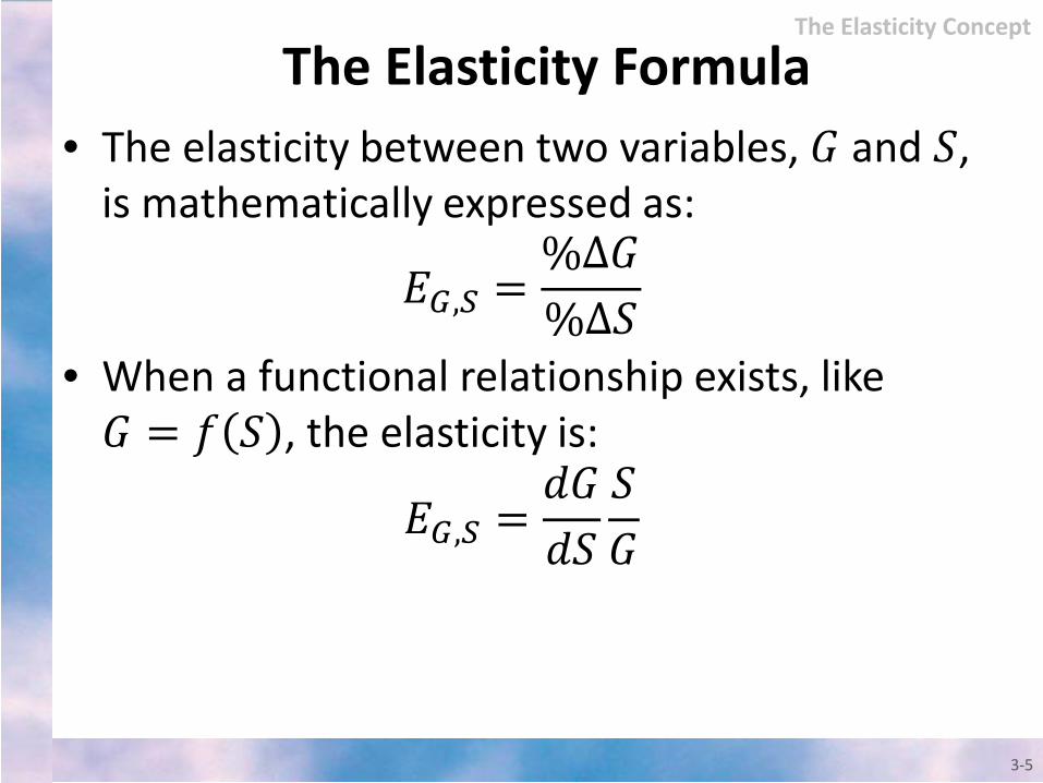
The Elasticity Formula • The elasticity between two variables, 𝐺𝐺 and 𝑆𝑆,

is mathematically expressed as:

𝐸𝐸𝐺𝐺,𝑆𝑆 =%Δ𝐺𝐺%Δ𝑆𝑆

• When a functional relationship exists, like 𝐺𝐺 = 𝑓𝑓 𝑆𝑆 , the elasticity is:

𝐸𝐸𝐺𝐺,𝑆𝑆 =𝑑𝑑𝐺𝐺𝑑𝑑𝑆𝑆

𝑆𝑆𝐺𝐺

3-5


Measurement Aspects of Elasticity • Important aspects of the elasticity:

– Sign of the relationship: • Positive. • Negative.

– Absolute value of elasticity magnitude relative to unity:

• 𝐸𝐸𝐺𝐺,𝑆𝑆 > 1 𝐺𝐺 is highly responsive to changes in 𝑆𝑆.

• 𝐸𝐸𝐺𝐺,𝑆𝑆 < 1 𝐺𝐺 is slightly responsive to changes in 𝑆𝑆.

3-6


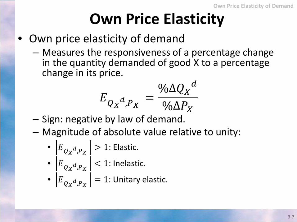
Own Price Elasticity • Own price elasticity of demand

– Measures the responsiveness of a percentage change in the quantity demanded of good X to a percentage change in its price.

𝐸𝐸𝑄𝑄𝑋𝑋𝑑𝑑,𝑃𝑃𝑋𝑋 =%Δ𝑄𝑄𝑋𝑋𝑑𝑑

%Δ𝑃𝑃𝑋𝑋

– Sign: negative by law of demand. – Magnitude of absolute value relative to unity:

• 𝐸𝐸𝑄𝑄𝑋𝑋𝑑𝑑,𝑃𝑃𝑋𝑋 > 1: Elastic.

• 𝐸𝐸𝑄𝑄𝑋𝑋𝑑𝑑,𝑃𝑃𝑋𝑋 < 1: Inelastic.

• 𝐸𝐸𝑄𝑄𝑋𝑋𝑑𝑑,𝑃𝑃𝑋𝑋 = 1: Unitary elastic.

3-7

Own Price Elasticity of Demand

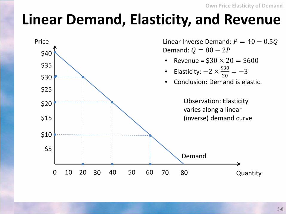
Linear Demand, Elasticity, and Revenue

3-8

Quantity

Price

Demand

$40

0

$20

$10

20 30

$5

40

$15

$30

$25

$35

10 50 60 70 80

Linear Inverse Demand: 𝑃𝑃 = 40 − 0.5𝑄𝑄 Demand: 𝑄𝑄 = 80 − 2𝑃𝑃 • Revenue = $30 × 20 = $600 • Elasticity: −2 × $30

20= −3

• Conclusion: Demand is elastic.

Observation: Elasticity varies along a linear (inverse) demand curve


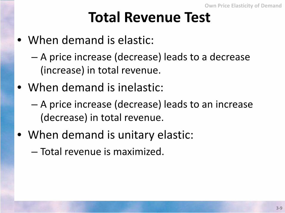
Total Revenue Test • When demand is elastic:

– A price increase (decrease) leads to a decrease (increase) in total revenue.

• When demand is inelastic: – A price increase (decrease) leads to an increase

(decrease) in total revenue.

• When demand is unitary elastic: – Total revenue is maximized.

3-9


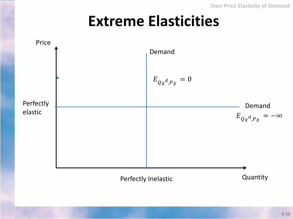
Extreme Elasticities

3-10

Quantity

Demand

Price

Perfectly Inelastic

𝐸𝐸𝑄𝑄𝑋𝑋𝑑𝑑,𝑃𝑃𝑋𝑋 = 0

Demand

𝐸𝐸𝑄𝑄𝑋𝑋𝑑𝑑,𝑃𝑃𝑋𝑋 = −∞

Perfectly elastic


Factors Affecting the Own Price Elasticity • Three factors can impact the own price

elasticity of demand: – Availability of consumption substitutes. – Time/Duration of purchase horizon. – Expenditure share of consumers’ budgets.

3-11


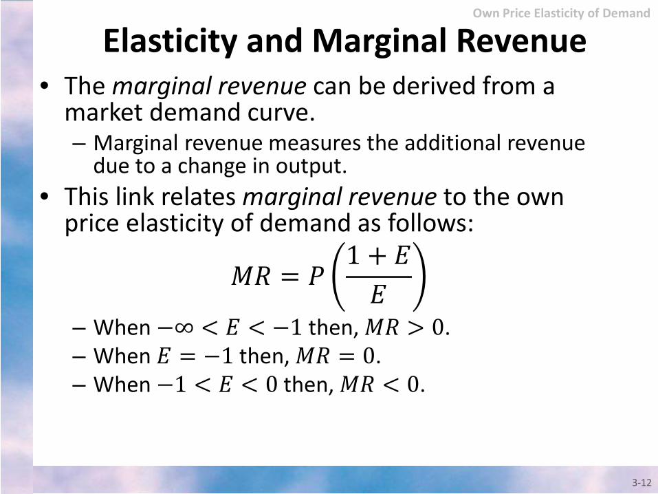
Elasticity and Marginal Revenue • The marginal revenue can be derived from a

market demand curve. – Marginal revenue measures the additional revenue

due to a change in output. • This link relates marginal revenue to the own

price elasticity of demand as follows:

𝑀𝑀𝑀𝑀 = 𝑃𝑃1 + 𝐸𝐸𝐸𝐸

– When −∞ < 𝐸𝐸 < −1 then, 𝑀𝑀𝑀𝑀 > 0. – When 𝐸𝐸 = −1 then, 𝑀𝑀𝑀𝑀 = 0. – When −1 < 𝐸𝐸 < 0 then, 𝑀𝑀𝑀𝑀 < 0.

3-12


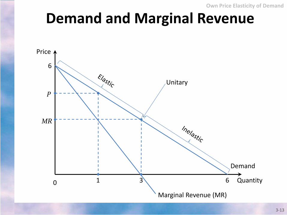
Demand and Marginal Revenue

3-13

Quantity 0

𝑃𝑃

MR

3

Price

6

Demand


1

6

Unitary

Marginal Revenue (MR)

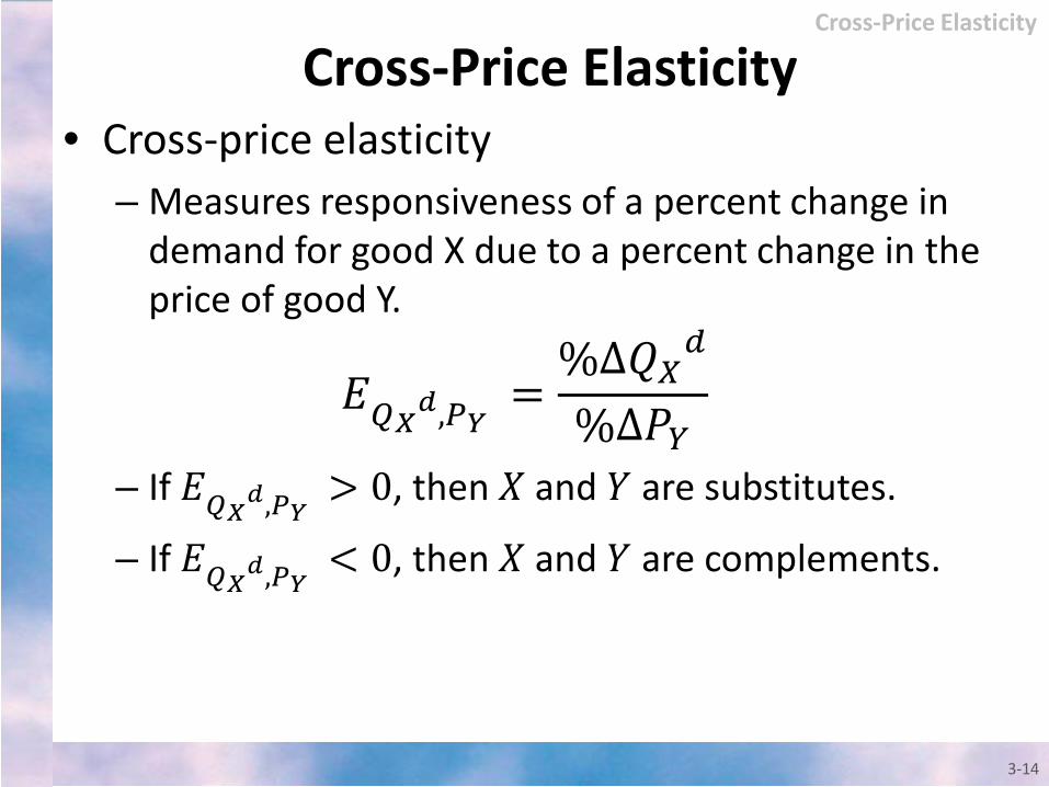
Cross-Price Elasticity • Cross-price elasticity

– Measures responsiveness of a percent change in demand for good X due to a percent change in the price of good Y.

𝐸𝐸𝑄𝑄𝑋𝑋𝑑𝑑,𝑃𝑃𝑌𝑌 =%Δ𝑄𝑄𝑋𝑋𝑑𝑑

%Δ𝑃𝑃𝑌𝑌

– If 𝐸𝐸𝑄𝑄𝑋𝑋𝑑𝑑,𝑃𝑃𝑌𝑌 > 0, then 𝑋𝑋 and 𝑌𝑌 are substitutes.

– If 𝐸𝐸𝑄𝑄𝑋𝑋𝑑𝑑,𝑃𝑃𝑌𝑌 < 0, then 𝑋𝑋 and 𝑌𝑌 are complements.

3-14

Cross-Price Elasticity

Cross-Price Elasticity in Action • Suppose it is estimated that the cross-price

elasticity of demand between clothing and food is -0.18. If the price of food is projected to increase by 10 percent, by how much will demand for clothing change?

−0.18 =%∆𝑄𝑄𝐶𝐶𝐶𝐶𝐶𝐶𝐶𝐶𝐶𝐶𝐶𝐶𝐶𝐶𝐶𝑑𝑑

10⇒ %∆𝑄𝑄𝐶𝐶𝐶𝐶𝐶𝐶𝐶𝐶𝐶𝐶𝐶𝐶𝐶𝐶𝐶𝑑𝑑 = −1.8

– That is, demand for clothing is expected to decline by 1.8 percent when the price of food increases 10 percent.

3-15


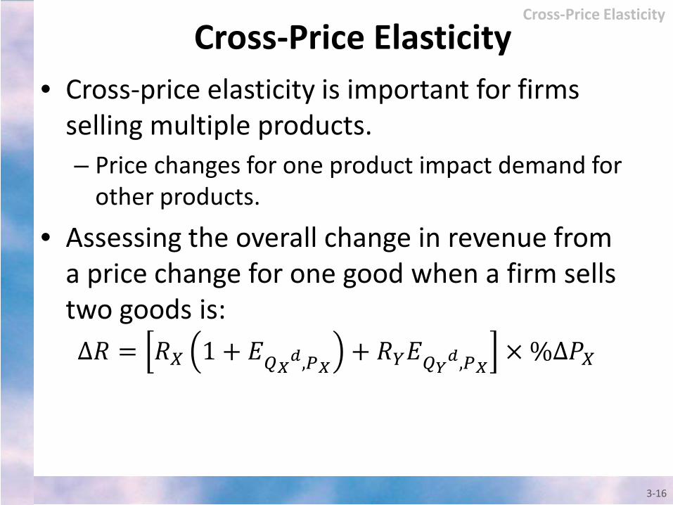
Cross-Price Elasticity • Cross-price elasticity is important for firms

selling multiple products. – Price changes for one product impact demand for

other products.

• Assessing the overall change in revenue from a price change for one good when a firm sells two goods is: ∆𝑀𝑀 = 𝑀𝑀𝑋𝑋 1 + 𝐸𝐸𝑄𝑄𝑋𝑋𝑑𝑑,𝑃𝑃𝑋𝑋

+ 𝑀𝑀𝑌𝑌𝐸𝐸𝑄𝑄𝑌𝑌𝑑𝑑,𝑃𝑃𝑋𝑋× %∆𝑃𝑃𝑋𝑋

3-16


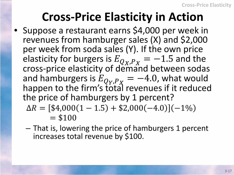
Cross-Price Elasticity in Action • Suppose a restaurant earns $4,000 per week in

revenues from hamburger sales (X) and $2,000 per week from soda sales (Y). If the own price elasticity for burgers is 𝐸𝐸𝑄𝑄𝑋𝑋,𝑃𝑃𝑋𝑋 = −1.5 and the cross-price elasticity of demand between sodas and hamburgers is 𝐸𝐸𝑄𝑄𝑌𝑌,𝑃𝑃𝑋𝑋 = −4.0, what would happen to the firm’s total revenues if it reduced the price of hamburgers by 1 percent? ∆𝑀𝑀 = $4,000 1 − 1.5 + $2,000 −4.0 −1%

= $100 – That is, lowering the price of hamburgers 1 percent

increases total revenue by $100.

3-17


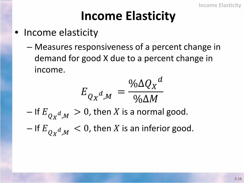
Income Elasticity • Income elasticity

– Measures responsiveness of a percent change in demand for good X due to a percent change in income.

𝐸𝐸𝑄𝑄𝑋𝑋𝑑𝑑,𝑀𝑀 =%Δ𝑄𝑄𝑋𝑋𝑑𝑑

%Δ𝑀𝑀

– If 𝐸𝐸𝑄𝑄𝑋𝑋𝑑𝑑,𝑀𝑀 > 0, then 𝑋𝑋 is a normal good.

– If 𝐸𝐸𝑄𝑄𝑋𝑋𝑑𝑑,𝑀𝑀 < 0, then 𝑋𝑋 is an inferior good.

3-18

Income Elasticity

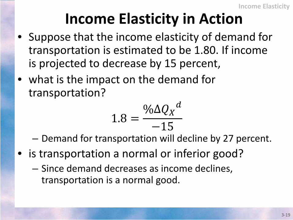
Income Elasticity in Action • Suppose that the income elasticity of demand for

transportation is estimated to be 1.80. If income is projected to decrease by 15 percent,

• what is the impact on the demand for transportation?

1.8 =%Δ𝑄𝑄𝑋𝑋𝑑𝑑

−15

– Demand for transportation will decline by 27 percent. • is transportation a normal or inferior good?

– Since demand decreases as income declines, transportation is a normal good.

3-19

Income Elasticity

Other Elasticities • Own advertising elasticity of demand for good X

is the ratio of the percentage change in the consumption of X to the percentage change in advertising spent on X.

• Cross-advertising elasticity between goods X and Y would measure the percentage change in the consumption of X that results from a 1 percent change in advertising toward Y.

3-20

Other Elasticities

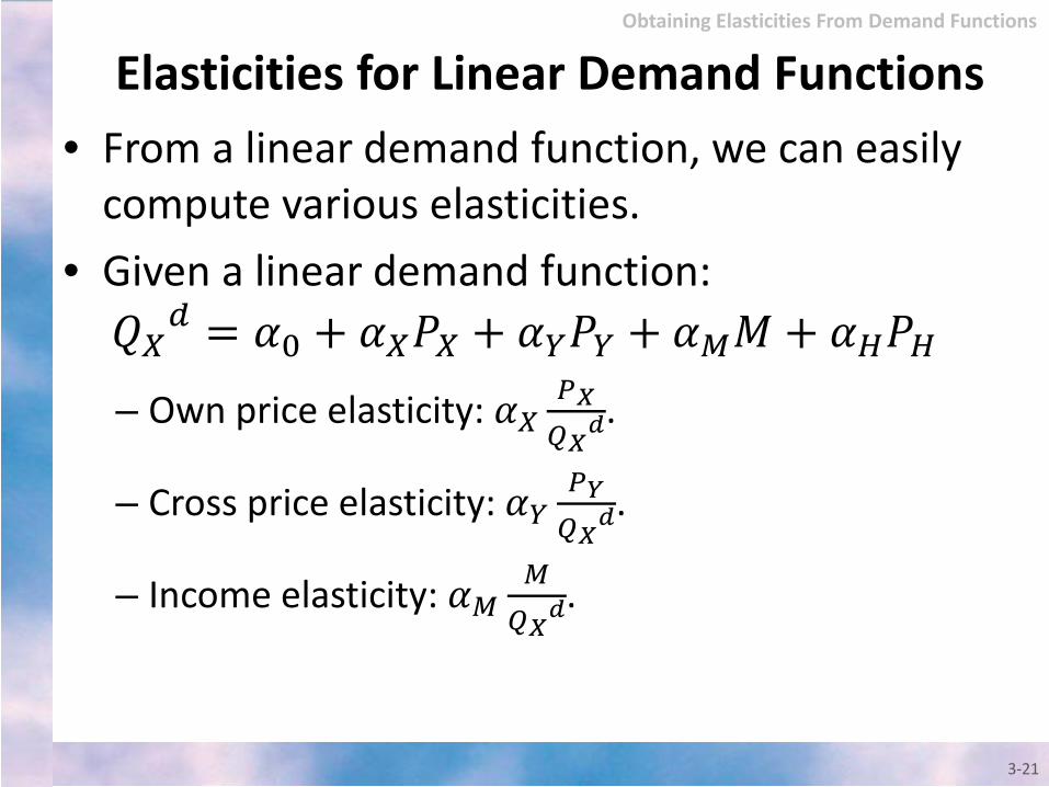
Elasticities for Linear Demand Functions • From a linear demand function, we can easily

compute various elasticities. • Given a linear demand function: 𝑄𝑄𝑋𝑋𝑑𝑑 = 𝛼𝛼0 + 𝛼𝛼𝑋𝑋𝑃𝑃𝑋𝑋 + 𝛼𝛼𝑌𝑌𝑃𝑃𝑌𝑌 + 𝛼𝛼𝑀𝑀𝑀𝑀 + 𝛼𝛼𝐻𝐻𝑃𝑃𝐻𝐻

– Own price elasticity: 𝛼𝛼𝑋𝑋𝑃𝑃𝑋𝑋𝑄𝑄𝑋𝑋𝑑𝑑

.

– Cross price elasticity: 𝛼𝛼𝑌𝑌𝑃𝑃𝑌𝑌𝑄𝑄𝑋𝑋𝑑𝑑

.

– Income elasticity: 𝛼𝛼𝑀𝑀𝑀𝑀𝑄𝑄𝑋𝑋𝑑𝑑

.

3-21

Obtaining Elasticities From Demand Functions

Elasticities for Linear Demand Functions In Action • The daily demand for Invigorated PED shoes is estimated to

be 𝑄𝑄𝑋𝑋𝑑𝑑 = 100 − 3𝑃𝑃𝑋𝑋 + 4𝑃𝑃𝑌𝑌 − 0.01𝑀𝑀 + 2𝐴𝐴𝑋𝑋

Suppose good X sells at $25 a pair, good Y sells at $35, the company utilizes 50 units of advertising, and average consumer income is $20,000. Calculate the own price, cross-price and income elasticities of demand. – 𝑄𝑄𝑋𝑋𝑑𝑑 = 100− 3 $25 + 4 $35 − 0.01 $20,000 + 2 50 =

65 units. – Own price elasticity: −3 25

65= −1.15.

– Cross-price elasticity: 4 3565

= 2.15.

– Income elasticity: −0.01 20,00065

= −3.08.

3-22


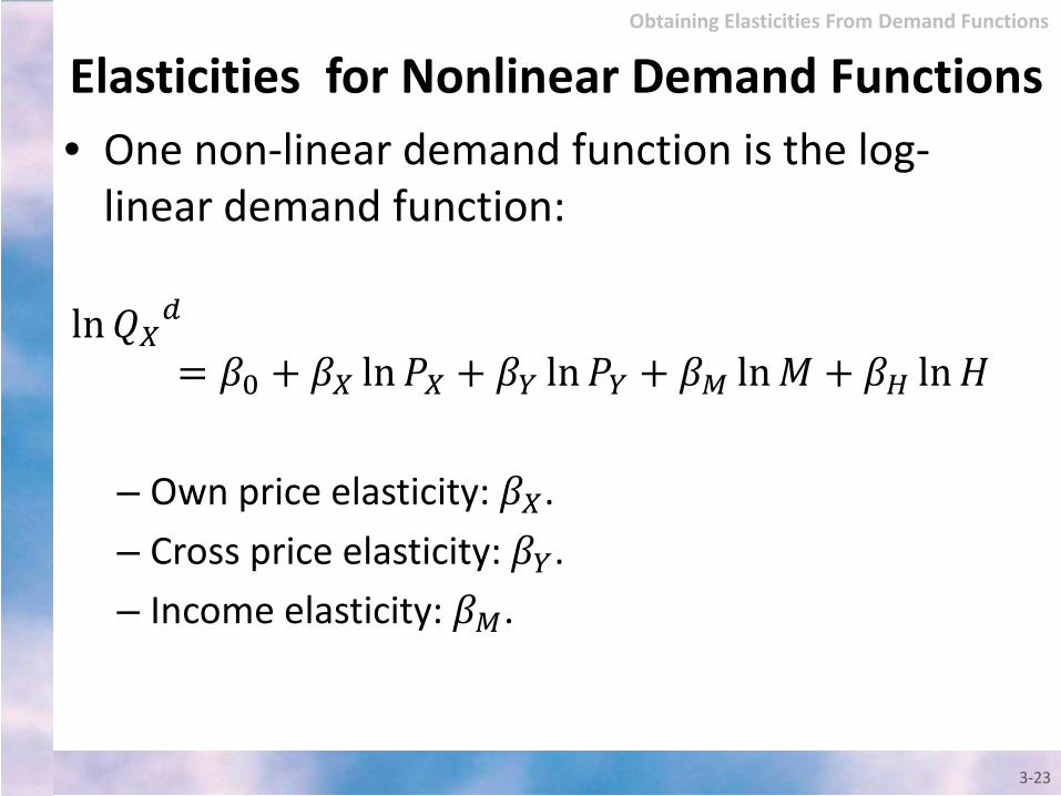
Elasticities for Nonlinear Demand Functions • One non-linear demand function is the log-

linear demand function: ln𝑄𝑄𝑋𝑋𝑑𝑑

= 𝛽𝛽0 + 𝛽𝛽𝑋𝑋 ln𝑃𝑃𝑋𝑋 + 𝛽𝛽𝑌𝑌 ln𝑃𝑃𝑌𝑌 + 𝛽𝛽𝑀𝑀 ln𝑀𝑀 + 𝛽𝛽𝐻𝐻 ln𝐻𝐻 – Own price elasticity: 𝛽𝛽𝑋𝑋. – Cross price elasticity: 𝛽𝛽𝑌𝑌. – Income elasticity: 𝛽𝛽𝑀𝑀.

3-23


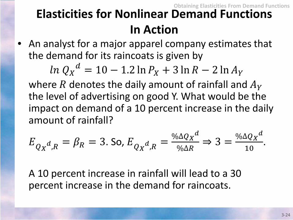
Elasticities for Nonlinear Demand Functions In Action

• An analyst for a major apparel company estimates that the demand for its raincoats is given by

𝑙𝑙𝑙𝑙 𝑄𝑄𝑋𝑋𝑑𝑑 = 10 − 1.2 ln𝑃𝑃𝑋𝑋 + 3 ln𝑀𝑀 − 2 ln𝐴𝐴𝑌𝑌 where 𝑀𝑀 denotes the daily amount of rainfall and 𝐴𝐴𝑌𝑌 the level of advertising on good Y. What would be the impact on demand of a 10 percent increase in the daily amount of rainfall?

𝐸𝐸𝑄𝑄𝑋𝑋𝑑𝑑,𝑅𝑅 = 𝛽𝛽𝑅𝑅 = 3. So, 𝐸𝐸𝑄𝑄𝑋𝑋𝑑𝑑,𝑅𝑅 = %∆𝑄𝑄𝑋𝑋𝑑𝑑

%∆𝑅𝑅⇒ 3 = %∆𝑄𝑄𝑋𝑋𝑑𝑑

10.

A 10 percent increase in rainfall will lead to a 30 percent increase in the demand for raincoats.

3-24


Regression Analysis • How does one obtain information on the

demand function? – Published studies. – Hire consultant. – Statistical technique called regression analysis

using data on quantity, price, income and other important variables.

3-25

Regression Analysis

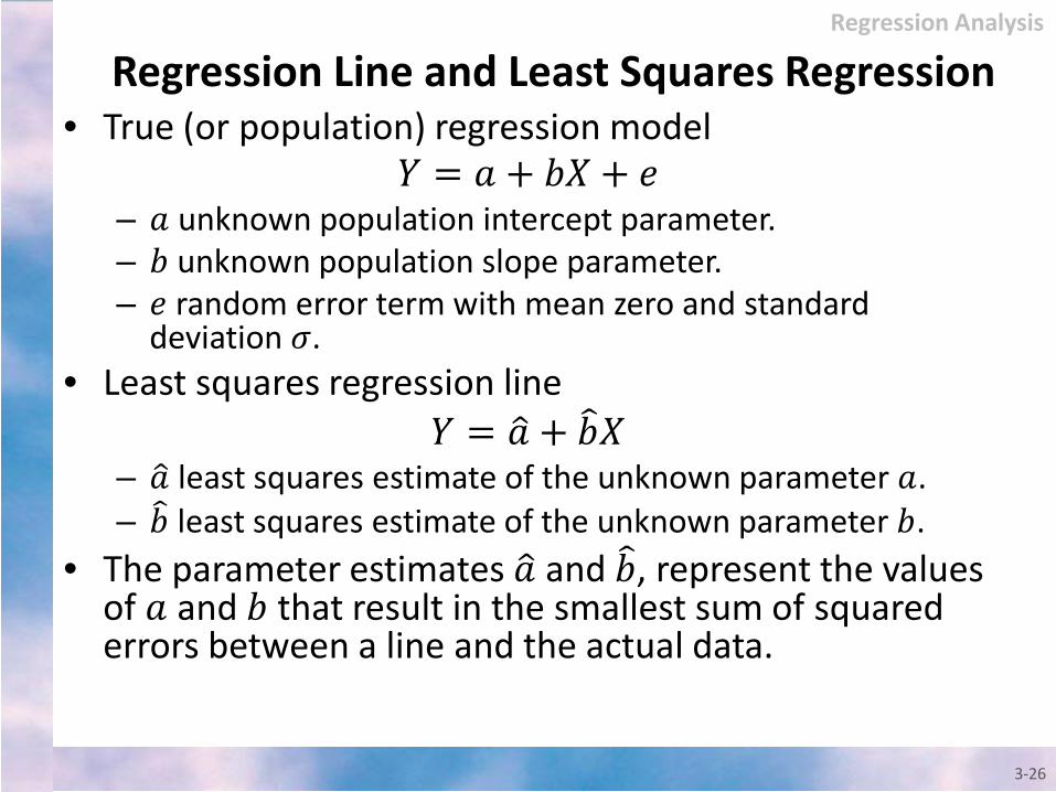
Regression Line and Least Squares Regression • True (or population) regression model

𝑌𝑌 = 𝑎𝑎 + 𝑏𝑏𝑋𝑋 + 𝑒𝑒 – 𝑎𝑎 unknown population intercept parameter. – 𝑏𝑏 unknown population slope parameter. – 𝑒𝑒 random error term with mean zero and standard

deviation 𝜎𝜎. • Least squares regression line

𝑌𝑌 = 𝑎𝑎� + 𝑏𝑏�𝑋𝑋 – 𝑎𝑎� least squares estimate of the unknown parameter 𝑎𝑎. – 𝑏𝑏� least squares estimate of the unknown parameter 𝑏𝑏.

• The parameter estimates 𝑎𝑎� and 𝑏𝑏�, represent the values of 𝑎𝑎 and 𝑏𝑏 that result in the smallest sum of squared errors between a line and the actual data.

3-26

Regression Analysis

Excel and Least Squares Estimates

3-27

SUMMARY OUTPUT

Regression Statistics Multiple R 0.87 R Square 0.75 Adjusted R Square 0.72 Standard Error 112.22 Observations 10.00

ANOVA Df SS MS F Significance F

Regression 1 301470.89 301470.89 23.94 0.0012 Residual 8 100751.61 12593.95 Total 9 402222.50

Coefficients Standard Error t Stat P-value Lower 95% Upper 95% Intercept 1631.47 243.97 6.69 0.0002 1068.87 2194.07 Price -2.60 0.53 -4.89 0.0012 -3.82 -1.37

Estimated Demand: 𝑄𝑄 = 1631.47 − 2.60𝑃𝑃𝑀𝑀𝑃𝑃𝑃𝑃𝐸𝐸

𝑎𝑎� = 1631.47 𝑏𝑏� = −2.60

Regression Analysis

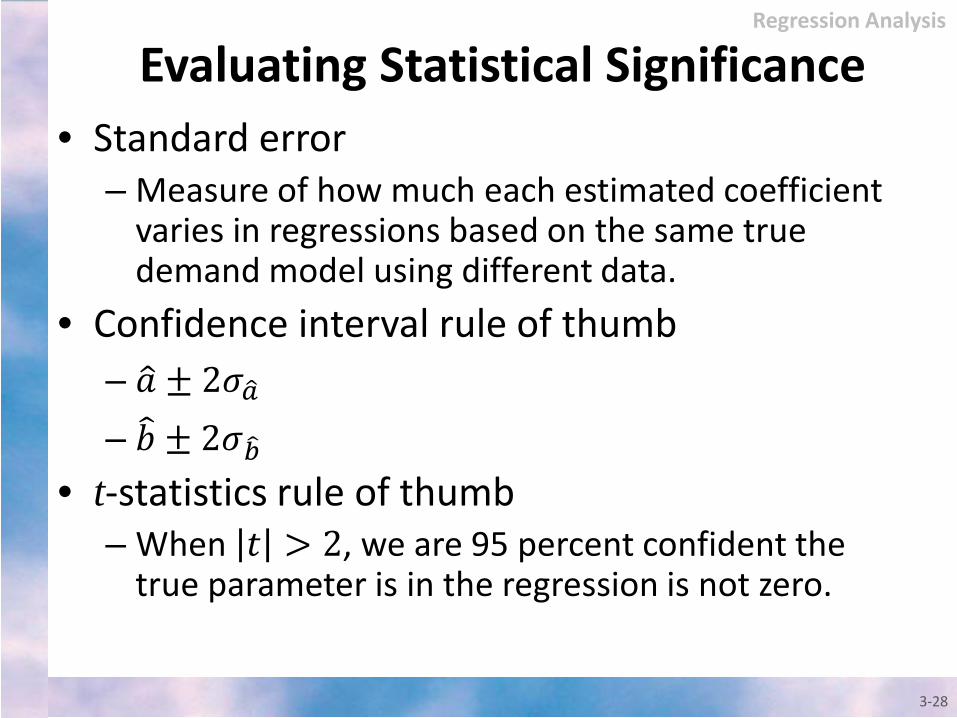
Evaluating Statistical Significance • Standard error

– Measure of how much each estimated coefficient varies in regressions based on the same true demand model using different data.

• Confidence interval rule of thumb – 𝑎𝑎� ± 2𝜎𝜎𝑎𝑎� – 𝑏𝑏� ± 2𝜎𝜎𝑏𝑏�

• t-statistics rule of thumb – When 𝑡𝑡 > 2, we are 95 percent confident the

true parameter is in the regression is not zero.

3-28

Regression Analysis


3-29

SUMMARY OUTPUT





Regression Analysis

𝑠𝑠𝑒𝑒 (𝑎𝑎)� = 243.97 𝑠𝑠𝑒𝑒(𝑏𝑏)� = 0.53

𝑡𝑡𝑎𝑎� = 6.69 > 2, the intercept is different from zero. 𝑡𝑡𝑏𝑏� = −4.89 < 2, the intercept is different from zero.

Evaluating Overall Regression Line Fit: R- Square

• R-Square – Also called the coefficient of determination. – Fraction of the total variation in the dependent

variable that is explained by the regression.

𝑀𝑀2 =𝐸𝐸𝐸𝐸𝐸𝐸𝑙𝑙𝑎𝑎𝐸𝐸𝑙𝑙𝑒𝑒𝑑𝑑 𝑉𝑉𝑎𝑎𝑉𝑉𝐸𝐸𝑎𝑎𝑡𝑡𝐸𝐸𝑉𝑉𝑙𝑙𝑇𝑇𝑉𝑉𝑡𝑡𝑎𝑎𝑙𝑙 𝑉𝑉𝑎𝑎𝑉𝑉𝐸𝐸𝑎𝑎𝑡𝑡𝐸𝐸𝑉𝑉𝑙𝑙

=𝑆𝑆𝑆𝑆𝑅𝑅𝑅𝑅𝐶𝐶𝑅𝑅𝑅𝑅𝑅𝑅𝑅𝑅𝐶𝐶𝐶𝐶𝐶𝐶𝑆𝑆𝑆𝑆𝑇𝑇𝐶𝐶𝐶𝐶𝑎𝑎𝐶𝐶

– Ranges between 0 and 1.

• Values closer to 1 indicate “better” fit.

3-30

Regression Analysis

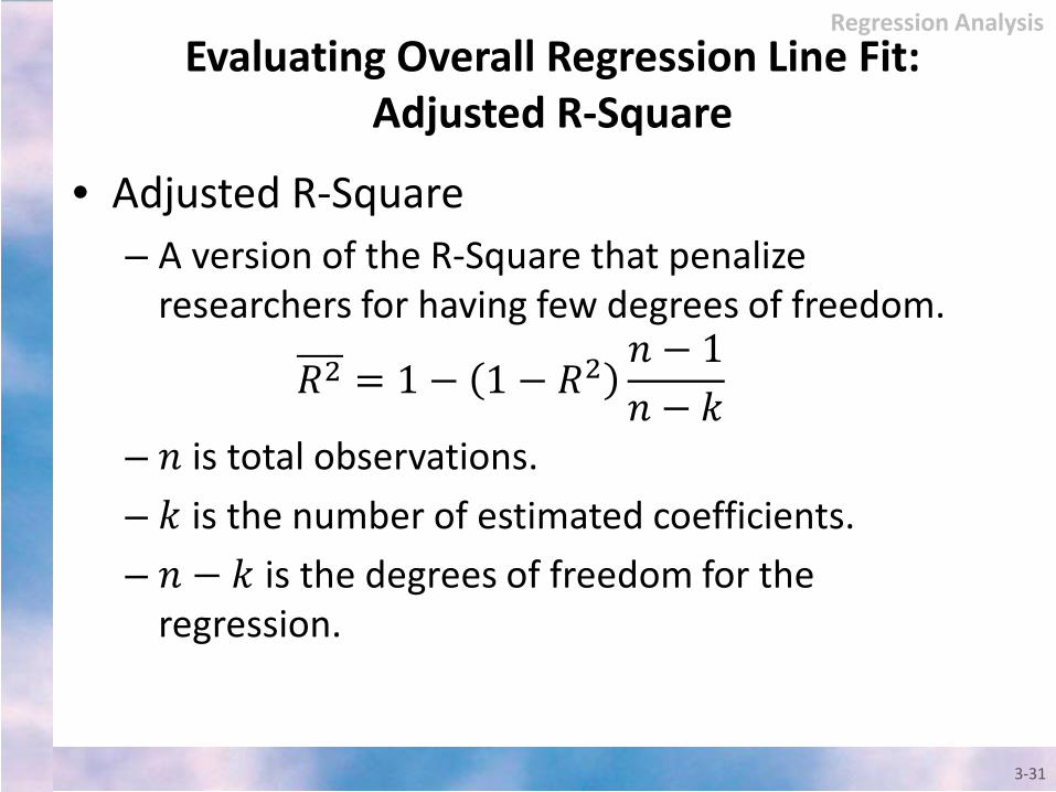
Evaluating Overall Regression Line Fit: Adjusted R-Square

• Adjusted R-Square – A version of the R-Square that penalize

researchers for having few degrees of freedom.

𝑀𝑀2 = 1 − 1 − 𝑀𝑀2𝑙𝑙 − 1𝑙𝑙 − 𝑘𝑘

– 𝑙𝑙 is total observations. – 𝑘𝑘 is the number of estimated coefficients. – 𝑙𝑙 − 𝑘𝑘 is the degrees of freedom for the

regression.

3-31

Regression Analysis

Evaluating Overall Regression Line Fit: F-Statistic

• A measure of the total variation explained by the regression relative to the total unexplained variation. – The greater the F-statistic, the better the overall

regression fit. – Equivalently, the P-value is another measure of the

F-statistic. • Lower p-values are associated with better overall

regression fit.

3-32

Regression Analysis


3-33

SUMMARY OUTPUT





Regression Analysis

Regression for Nonlinear Functions and Multiple Regression

• Regression techniques can also be applied to the following settings: – Nonlinear functional relationships:

• Nonlinear regression example: ln𝑄𝑄 = 𝛽𝛽0 + 𝛽𝛽𝑝𝑝 ln𝑃𝑃 + 𝑒𝑒

– Functional relationships with multiple variables: • Multiple regression example: 𝑄𝑄𝑋𝑋𝑑𝑑 = 𝛼𝛼0 + 𝛼𝛼𝑋𝑋𝑃𝑃𝑋𝑋 + 𝛼𝛼𝑀𝑀𝑀𝑀 + 𝛼𝛼𝐻𝐻𝑃𝑃𝐻𝐻 + 𝑒𝑒

or ln𝑄𝑄𝑋𝑋𝑑𝑑 = 𝛽𝛽0 + 𝛽𝛽𝑋𝑋 ln𝑃𝑃𝑋𝑋 + 𝛽𝛽𝑀𝑀 ln𝑀𝑀 + 𝛽𝛽𝐻𝐻 ln𝑃𝑃𝐻𝐻 + 𝑒𝑒

3-34

Regression Analysis


3-35

SUMMARY OUTPUT




Coefficients Standard Error t Stat P-value Lower 95% Upper 95% Intercept 135.15 20.65 6.54 0.0006 84.61 185.68 Price -0.14 0.06 -2.41 0.0500 -0.29 0.00 Advertising 0.54 0.64 0.85 0.4296 -1.02 2.09 Distance -5.78 1.26 -4.61 0.0037 -8.86 -2.71

Regression Analysis

Conclusion • Elasticities are tools you can use to quantify

the impact of changes in prices, income, and advertising on sales and revenues.

• Given market or survey data, regression analysis can be used to estimate: – Demand functions. – Elasticities. – A host of other things, including cost functions.

• Managers can quantify the impact of changes in prices, income, advertising, etc.

3-36

Documents

Quantitative Demand Analysis - MyWeb 2015/IPPTChap003… · • Chapter 2 focused on interpreting demand ... – An increase in the price of a good leads quantity demanded for that