IV Conferencia Panamericana de END Buenos Aires – Octubre 2007

Quantitative Analysis of Eddy Current NDE Data

Y. M. Kim, E. C. Johnson, O. Esquivel The Aerospace Corporation, M2-248

P. O. Box 92957 Los Angeles, CA 90275, USA

310-336-7602 eric.c.johnson@aero.org

Abstract A new method for analyzing eddy current inspection data is presented. The key concept behind this method is extraction and isolation of the sample response from the measured signal. The measured signal depends on many factors including, not only the characteristics of the probe itself, the sample material, the operation frequency, and the probe/sample geometry, but also the measurement instrumentation and cabling. To start, complex impedance measurements of the (1) isolated probe and (2) probe with sample as a function of frequency were conducted. The data frequency dependence was found to exhibit resonance behavior that could be fit to a model RLC circuit. The validity of this model circuit was confirmed by the predictable resonance change upon introduction of additional capacitors into the measurement configuration. Without external capacitance, the value for C generally reflects the stray capacitances of the instruments and cables and, hence, is unaffected by presence of a sample. Furthermore, data at a fixed-frequency can be easily related to those of swept frequency measurements via a conformal mapping deduced from analysis of the model circuit. Using this approach, data from fixed-frequency measurements can be effectively mapped to a corrected R and ωL plane. Data for a variety of materials reveals sample responses that can be easily explained in terms of surface impedance variations. In addition, for this corrected R and ωL plane, lift-off behavior scales in a simple predictable fashion and data at different lift-off conditions can be analyzed to further reduce the properties of the sample. Furthermore, defects characteristics, such as crack width and depth, can be quantified with simple physical reasoning and the condition of multiple conductive layers can be evaluated. This improved understanding of the defect signals can be exploited for the design of more efficient probes that are matched to the materials under test. Moreover, this quantitative method allows one to present data taken with different probe and instrument settings in an invariant form representative of the fundamental surface impedance for the specimen. 1. Introduction Conventional eddy current NDE methods generally involve measurement of the real and imaginary components of the electrical AC impedance of a probe coil at a fixed frequency, with the results plotted in a complex plane. In this representation of signals, the signal point varies in its position depending on the electromagnetic properties of the test sample and the degree of the proximity between the probe and the sample. The presence of localized defects (such as cracks), and potentially detrimental material variations (i.e., stress induced deformation, grind-burn, variation in grain texture, etc.)

Support for this work under The Aerospace Corporation Independent Research and Development Program is gratefully acknowledged.

© 2007 The Aerospace Corporation

IV Conferencia Panamericana de END Buenos Aires – Octubre 2007 2

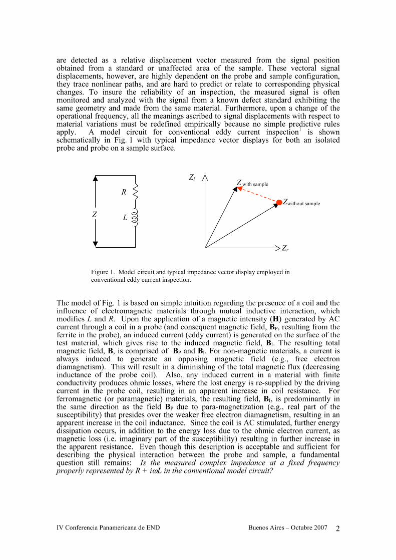
are detected as a relative displacement vector measured from the signal position obtained from a standard or unaffected area of the sample. These vectoral signal displacements, however, are highly dependent on the probe and sample configuration, they trace nonlinear paths, and are hard to predict or relate to corresponding physical changes. To insure the reliability of an inspection, the measured signal is often monitored and analyzed with the signal from a known defect standard exhibiting the same geometry and made from the same material. Furthermore, upon a change of the operational frequency, all the meanings ascribed to signal displacements with respect to material variations must be redefined empirically because no simple predictive rules apply. A model circuit for conventional eddy current inspection1 is shown schematically in Fig. 1 with typical impedance vector displays for both an isolated probe and probe on a sample surface. The model of Fig. 1 is based on simple intuition regarding the presence of a coil and the influence of electromagnetic materials through mutual inductive interaction, which modifies L and R. Upon the application of a magnetic intensity (H) generated by AC current through a coil in a probe (and consequent magnetic field, BP, resulting from the ferrite in the probe), an induced current (eddy current) is generated on the surface of the test material, which gives rise to the induced magnetic field, BI. The resulting total magnetic field, B, is comprised of BP and BI. For non-magnetic materials, a current is always induced to generate an opposing magnetic field (e.g., free electron diamagnetism). This will result in a diminishing of the total magnetic flux (decreasing inductance of the probe coil). Also, any induced current in a material with finite conductivity produces ohmic losses, where the lost energy is re-supplied by the driving current in the probe coil, resulting in an apparent increase in coil resistance. For ferromagnetic (or paramagnetic) materials, the resulting field, BI, is predominantly in the same direction as the field BP due to para-magnetization (e.g., real part of the susceptibility) that presides over the weaker free electron diamagnetism, resulting in an apparent increase in the coil inductance. Since the coil is AC stimulated, further energy dissipation occurs, in addition to the energy loss due to the ohmic electron current, as magnetic loss (i.e. imaginary part of the susceptibility) resulting in further increase in the apparent resistance. Even though this description is acceptable and sufficient for describing the physical interaction between the probe and sample, a fundamental question still remains: Is the measured complex impedance at a fixed frequency properly represented by R + iωL in the conventional model circuit?

Zi

Zr

Zwithout sample

Z with sample

Figure 1. Model circuit and typical impedance vector display employed in conventional eddy current inspection.

R

L Z

IV Conferencia Panamericana de END Buenos Aires – Octubre 2007 3

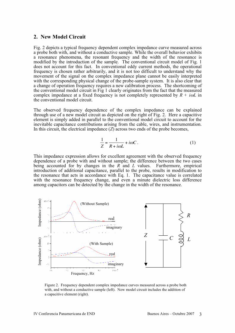
2. New Model Circuit Fig. 2 depicts a typical frequency dependent complex impedance curve measured across a probe both with, and without a conductive sample. While the overall behavior exhibits a resonance phenomena, the resonant frequency and the width of the resonance is modified by the introduction of the sample. The conventional circuit model of Fig. 1 does not account for this fact. In conventional eddy current methods, the operational frequency is chosen rather arbitrarily, and it is not too difficult to understand why the movement of the signal on the complex impedance plane cannot be easily interpreted with the corresponding physical change of the probe-sample system. It is also clear that a change of operation frequency requires a new calibration process. The shortcoming of the conventional model circuit in Fig 1 clearly originates from the fact that the measured complex impedance at a fixed frequency is not completely represented by R + iωL in the conventional model circuit. The observed frequency dependence of the complex impedance can be explained through use of a new model circuit as depicted on the right of Fig. 2. Here a capacitive element is simply added in parallel to the conventional model circuit to account for the inevitable capacitance contributions arising from the cable, wires, and instrumentation. In this circuit, the electrical impedance (Z) across two ends of the probe becomes,

!

1

Z=

1

R + i"L+ i"C . (1)

This impedance expression allows for excellent agreement with the observed frequency dependence of a probe with and without sample; the difference between the two cases being accounted for by changes in the R and L values. Furthermore, empirical introduction of additional capacitance, parallel to the probe, results in modification to the resonance that acts in accordance with Eq. 1. The capacitance value is correlated with the resonance frequency change, and even a minute dielectric loss difference among capacitors can be detected by the change in the width of the resonance.

L

Figure 2. Frequency dependent complex impedance curves measured across a probe both with, and without a conductive sample (left). New model circuit includes the addition of a capacitive element (right).

(Without Sample)

real

real

imaginary

(With Sample)

imaginary

C

R

Z

Impe

danc

e (o

hm)

Impe

danc

e (o

hm)

Frequency, Hz

IV Conferencia Panamericana de END Buenos Aires – Octubre 2007 4

To express the frequency dependence of Z(ω) and to make it simpler for deducing its characteristics in terms of R, L and C, Eq. 1 can be scaled with the following characteristic impedance, Z0, and frequency, f0, defined as

!

Z0"

L

C (2)

!

"0

= 2#f0$

1

LC. (3)

With these definitions, the resistance, R, and the frequency f!" 2= can be translated into dimensionless quantities by the following definitions:

!

" #R

Z0

, (4)

!

" #$

$0

=f

f0

. (5)

In terms of the parameters above, Eq. 1 becomes

!

Z(") = Z0

# + i"

(1$" 2) + i#" . (6)

The real and imaginary parts of this complex impedance can be written in as

2222

22

022220)1(

)1()( and

)1()(

!"!

"!!!

!"!

"!

+#

##=

+#= ZZZZ

ir . (7)

Assuming

!

" <<1 (i.e. R << #0) , from inspection of Eq. 7, the following frequency (ν)

dependant characteristics can be easily identified:

Zr(ν) is positive with the maximum value for f = f0 of

!

Zm"Z0

#=

L

RC.

Zi(ν) changes its sign about f = f0. More exactly, from the derivative of Eq. 7 with respect to ν, one can show that the maximum value of Zr and its frequency becomes

!

Max("r) = Z

r(#

max) = Z

m

1

1$1

4%2

&

' (

)

* +

, Zm1+

1

4%2

&

' (

)

* + (8)

with

!

"max

= 1#1

2$2 % 1#

1

4$2

&

' (

)

* + . (9)

IV Conferencia Panamericana de END Buenos Aires – Octubre 2007 5

At

!

" =1 , the components of Z become

!

" r (# =1) = Zm and " i (# =1) = $"0 . (10)

Furthermore at two well defined frequencies,

!

" =1±1

2# , the following can be shown

in first order of ρ:

!

" r (# =1±1

2$) %

1

2Zm 1±

1

2$

&

' (

)

* + %

1

2Zm and " i (# =1±

1

2$) % ±

1

2Zm (11)

Note that the absolute values of the real and imaginary parts of the complex impedance at these two frequencies become equal to the half value of the resonance peak, Zm. The interval of these two frequencies can be used as a definition of the resonance width, W.

!

W " f0# . (12)

In typical frequency dependant impedance measurement data, this resonance width can be identified by measuring the full half maximum width of Zr(f) or a full width at the 70.71% level %).%.( 717010050 =! in the impedance magnitude

!

Z( f ) . The quality factor of the resonance, Q, is defined as the ratio of the resonant frequency and the width of resonance, and becomes simply

!

Q "f0

W=1

# . (13)

The above definitions of Zm, f0 and W provide the measurable parameters from which the values of RLC in the model circuit can be uniquely identified. The swept frequency and fixed frequency conformal mapping methods described below are natural extensions of existing eddy current methodology to which this new circuit model can be applied for data analysis. 3. Swept Frequency Method For an AC current where the frequency is swept (using an AC voltage source and a large, serially connected load resistance), the amplitude of the AC voltage drop across the probe can be measured for

!

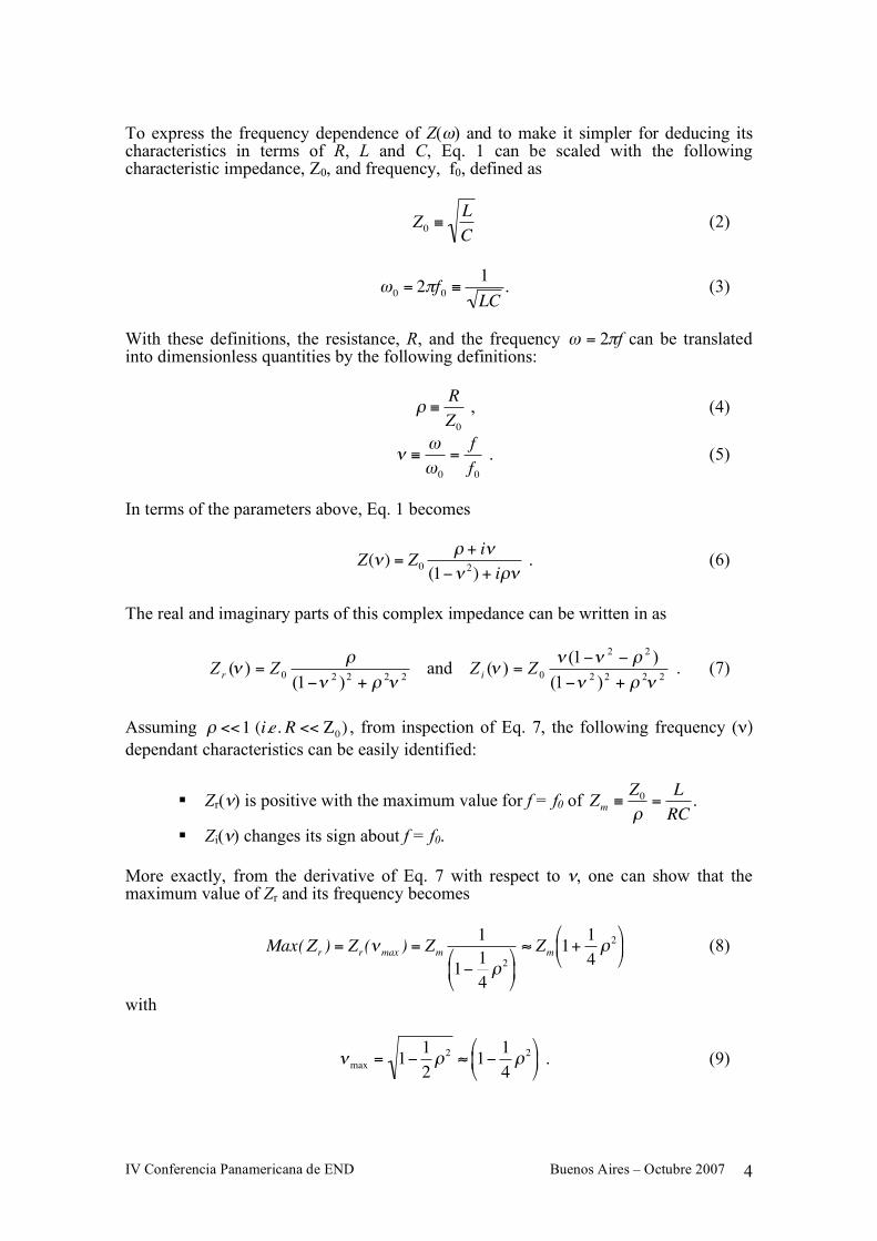
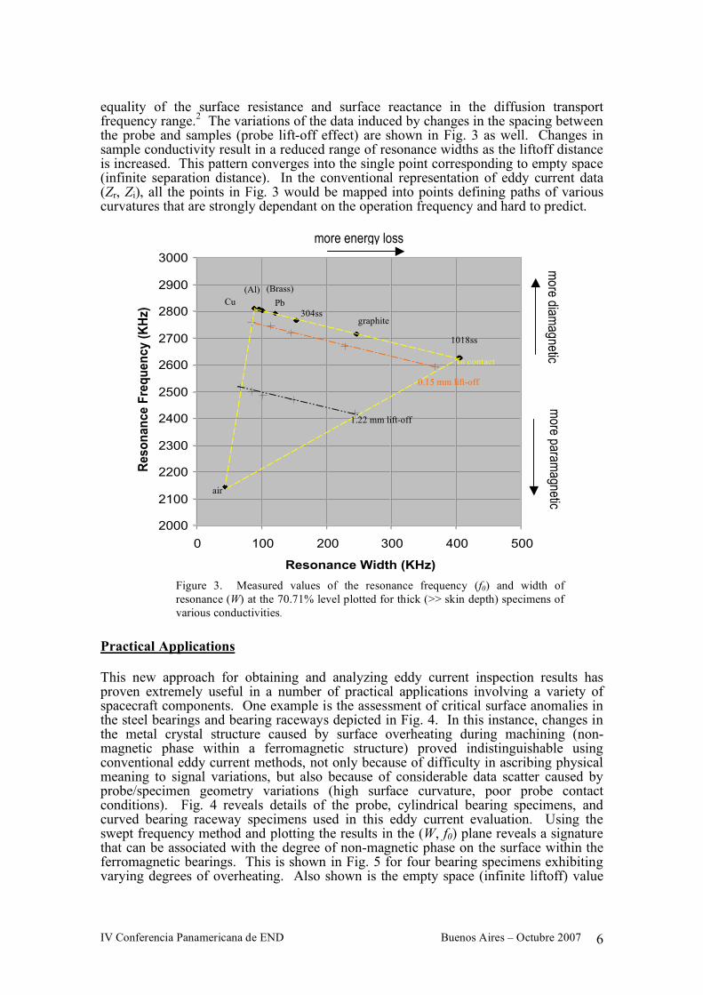
Z( f ) . The measured, frequency dependant, impedance magnitude reveals that the influence of the sample is manifested in a convolution of shifts in the resonance frequency and changes in the width of resonance. Alternatively, by fitting the data, one can calculate the corresponding sample influence in R and X≡ ω0L. Two-dimensional representation of the data in either (W, f0) or (R, X) coordinates are equivalently useful for understanding the physical meaning of the results. In Fig. 3, the resonance frequencies (f0), and widths of the resonance (W) at the 70.71% level of the peak value of

!

Z( f ) are plotted for specimens of various conductivities. The relationship between the variation in conductivity and the resultant variation between resonance frequency and width is a well-known phenomenon in the field of microwaves. Sample variations can be explained in the free electron theory by the

IV Conferencia Panamericana de END Buenos Aires – Octubre 2007 6

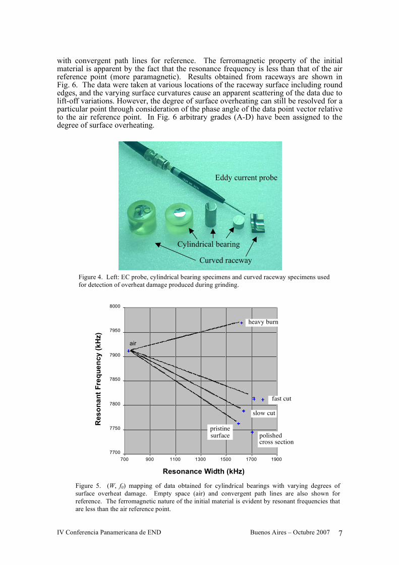
equality of the surface resistance and surface reactance in the diffusion transport frequency range.2 The variations of the data induced by changes in the spacing between the probe and samples (probe lift-off effect) are shown in Fig. 3 as well. Changes in sample conductivity result in a reduced range of resonance widths as the liftoff distance is increased. This pattern converges into the single point corresponding to empty space (infinite separation distance). In the conventional representation of eddy current data (Zr, Zi), all the points in Fig. 3 would be mapped into points defining paths of various curvatures that are strongly dependant on the operation frequency and hard to predict. Practical Applications This new approach for obtaining and analyzing eddy current inspection results has proven extremely useful in a number of practical applications involving a variety of spacecraft components. One example is the assessment of critical surface anomalies in the steel bearings and bearing raceways depicted in Fig. 4. In this instance, changes in the metal crystal structure caused by surface overheating during machining (non-magnetic phase within a ferromagnetic structure) proved indistinguishable using conventional eddy current methods, not only because of difficulty in ascribing physical meaning to signal variations, but also because of considerable data scatter caused by probe/specimen geometry variations (high surface curvature, poor probe contact conditions). Fig. 4 reveals details of the probe, cylindrical bearing specimens, and curved bearing raceway specimens used in this eddy current evaluation. Using the swept frequency method and plotting the results in the (W, f0) plane reveals a signature that can be associated with the degree of non-magnetic phase on the surface within the ferromagnetic bearings. This is shown in Fig. 5 for four bearing specimens exhibiting varying degrees of overheating. Also shown is the empty space (infinite liftoff) value

2000

2100

2200

2300

2400

2500

2600

2700

2800

2900

3000

0 100 200 300 400 500

Resonance Width (KHz)

Reso

nan

ce F

req

uen

cy (

KH

z)

0.15 mm lift-off

1.22 mm lift-off

In contact

air

(Al) Pb

(Brass) Cu

304ss

1018ss

graphite

Figure 3. Measured values of the resonance frequency (f0) and width of resonance (W) at the 70.71% level plotted for thick (>> skin depth) specimens of various conductivities.

more diam

agnetic m

ore paramagnetic

more energy loss

IV Conferencia Panamericana de END Buenos Aires – Octubre 2007 7

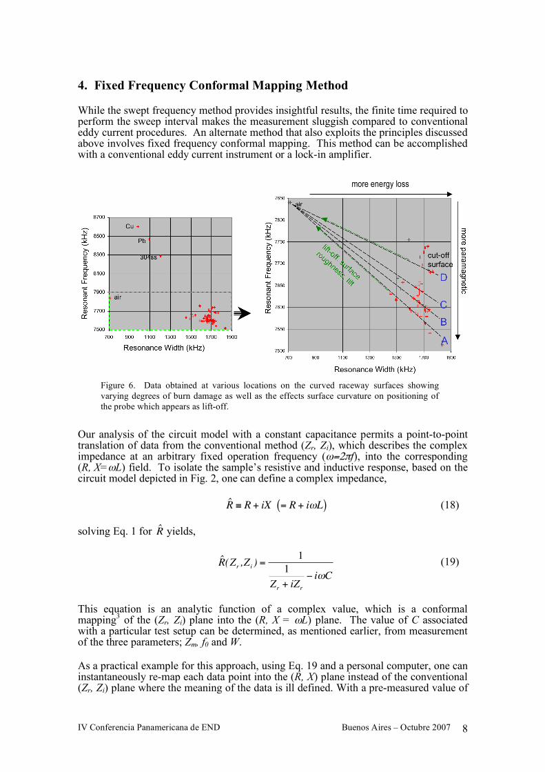
with convergent path lines for reference. The ferromagnetic property of the initial material is apparent by the fact that the resonance frequency is less than that of the air reference point (more paramagnetic). Results obtained from raceways are shown in Fig. 6. The data were taken at various locations of the raceway surface including round edges, and the varying surface curvatures cause an apparent scattering of the data due to lift-off variations. However, the degree of surface overheating can still be resolved for a particular point through consideration of the phase angle of the data point vector relative to the air reference point. In Fig. 6 arbitrary grades (A-D) have been assigned to the degree of surface overheating.

Figure 4. Left: EC probe, cylindrical bearing specimens and curved raceway specimens used for detection of overheat damage produced during grinding.

Figure 5. (W, f0) mapping of data obtained for cylindrical bearings with varying degrees of surface overheat damage. Empty space (air) and convergent path lines are also shown for reference. The ferromagnetic nature of the initial material is evident by resonant frequencies that are less than the air reference point.

7 7 0 0

7 7 5 0

7 8 0 0

7 8 5 0

7 9 0 0

7 9 5 0

8 0 0 0

7 0 0 9 0 0 1 1 0 0 1 3 0 0 1 5 0 0 1 7 0 0 1 9 0 0 R e s o n a n c e W i d t h ( K H z )

air

fast cut

heavy burn

slow cut

pristine surface polished

cross section

Resonance Width (kHz)

Res

onan

t Fre

quen

cy (k

Hz)

Eddy current probe

Curved raceway

Cylindrical bearing

IV Conferencia Panamericana de END Buenos Aires – Octubre 2007 8

4. Fixed Frequency Conformal Mapping Method While the swept frequency method provides insightful results, the finite time required to perform the sweep interval makes the measurement sluggish compared to conventional eddy current procedures. An alternate method that also exploits the principles discussed above involves fixed frequency conformal mapping. This method can be accomplished with a conventional eddy current instrument or a lock-in amplifier. Our analysis of the circuit model with a constant capacitance permits a point-to-point translation of data from the conventional method (Zr, Zi), which describes the complex impedance at an arbitrary fixed operation frequency (ω=2πf), into the corresponding (R, X=ωL) field. To isolate the sample’s resistive and inductive response, based on the circuit model depicted in Fig. 2, one can define a complex impedance,

!

ˆ R " R + iX = R + i#L( ) (18) solving Eq. 1 for

!

ˆ R yields,

!

ˆ R (Zr,Z

i) =

1

1

Zr+ iZ

r

" i#C

(19)

This equation is an analytic function of a complex value, which is a conformal mapping3 of the (Zr, Zi) plane into the (R, X = ωL) plane. The value of C associated with a particular test setup can be determined, as mentioned earlier, from measurement of the three parameters; Zm, f0 and W. As a practical example for this approach, using Eq. 19 and a personal computer, one can instantaneously re-map each data point into the (R, X) plane instead of the conventional (Zr, Zi) plane where the meaning of the data is ill defined. With a pre-measured value of

Figure 6. Data obtained at various locations on the curved raceway surfaces showing varying degrees of burn damage as well as the effects surface curvature on positioning of the probe which appears as lift-off.

more energy loss

IV Conferencia Panamericana de END Buenos Aires – Octubre 2007 9

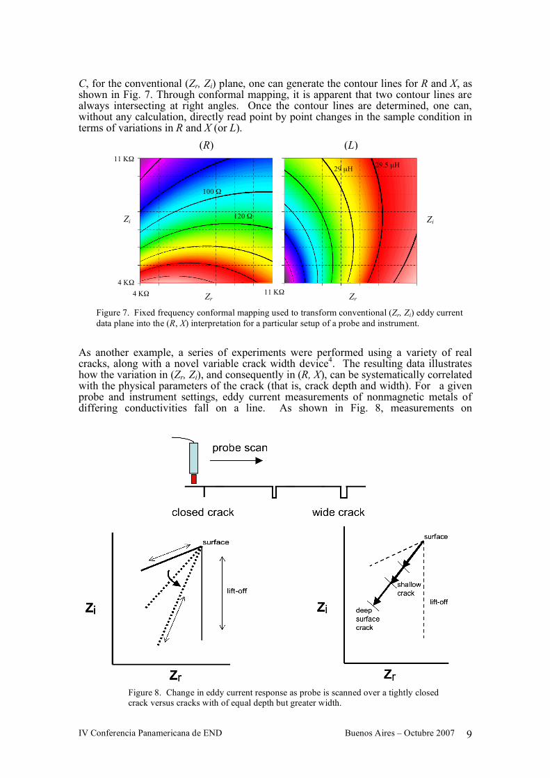
C, for the conventional (Zr, Zi) plane, one can generate the contour lines for R and X, as shown in Fig. 7. Through conformal mapping, it is apparent that two contour lines are always intersecting at right angles. Once the contour lines are determined, one can, without any calculation, directly read point by point changes in the sample condition in terms of variations in R and X (or L). As another example, a series of experiments were performed using a variety of real cracks, along with a novel variable crack width device4. The resulting data illustrates how the variation in (Zr, Zi), and consequently in (R, X), can be systematically correlated with the physical parameters of the crack (that is, crack depth and width). For a given probe and instrument settings, eddy current measurements of nonmagnetic metals of differing conductivities fall on a line. As shown in Fig. 8, measurements on

(R) (Zr, Zi)

(L) (Zr, Zi)

4

Zi

100 Ω

120 Ω

29.5 µH 29 µH

Zi

Zr Zr

11 KΩ

11 KΩ 4 KΩ

4 KΩ

Figure 7. Fixed frequency conformal mapping used to transform conventional (Zr, Zi) eddy current data plane into the (R, X) interpretation for a particular setup of a probe and instrument.

Figure 8. Change in eddy current response as probe is scanned over a tightly closed crack versus cracks with of equal depth but greater width.

IV Conferencia Panamericana de END Buenos Aires – Octubre 2007 10

tight cracks of varying depth fall approximately along the same line with increased displacement relative to the surface for deeper cracks. As the crack width increases, the response tends toward that of a pure lift off response. If one changes the probe or instrument settings, the behavior will be the same, but the response will be rotated and/or stretched. However, if one maps to the (R, X) plane, the results remain invariant according to Eq. 19. This perception resolves much of the confusion associated with changes that occur when different probes are used or instrument settings are altered. The conformal mapping of Eq. 19 was also used to great advantage in an examination of a number composite overwrapped pressure vessels (COPVs). These COPVs consisted of a thin aluminum liner overwrapped with hoop and helical layers of graphite fibers embedded in an epoxy matrix5 as depicted in Fig. 9. In these vessels, subsurface ply irregularities caused by subtle impact damage can greatly jeopardize ultimate strength. While the results of conventional (Zr, Zi) data, shown in Fig. 10, were insufficient for health assessment, subsequent conformal mapping into the (R, X) plane (shown in Fig. 11) provided enhanced resolution of the effective conductivity variations produced by ply orientation and resin density. The effect of the helical fibers is clearly visible in the images formed from the (R, X) plane.

Figure 9. Cross-section of a graphite epoxy COPV.

IV Conferencia Panamericana de END Buenos Aires – Octubre 2007 11

70 KΩ

40 KΩ

-40 KΩ

0

0Z r

Z i

10KΩ

10KΩ

70 KΩ

40 KΩ

-40 KΩ

0

0Z r

Z i

10KΩ

10KΩ

Figure 10. Data collected by scanning an anisotropic eddy current probe over a filament-wound COPV at a fixed frequency and presented in a conventional (Zr, Zi) mapping. The probe was designed to induce current normal to the top hoop ply. The rectangular mark at lower edge is due to movement of the probe due to a bump (excess epoxy) on the COPV surface.

COPV

scan Zr

Zi

Figure 11. Same scan data as Fig. 10 after conformal mapping to (X, R) plane. Note the enhanced helical fiber lay-up in the R amplitude image.

R

X

46 Ω 34 Ω

1640 Ω

1460 Ω

air

46 Ω 34 Ω

1640 Ω

1460 Ω

air

46 Ω 34 Ω

1640 Ω

1460 Ω

R

X

46 Ω 34 Ω

1640 Ω

1460 Ω

air

Al

1640 Ω

1460 Ω 34 Ω 46 Ω

IV Conferencia Panamericana de END Buenos Aires – Octubre 2007 12

5. Summary We have developed a new method for analyzing eddy current data through an improved model circuit accounting for the capacitive elements in the measurement process. This method permits one to extract the net sample response through the change in resistive and inductive impedance contributions. Through such representation, data variations can be directly linked to physical property changes in the materials and geometry. Two practical measurement and analysis methods are presented: (a) a frequency sweep method, and (b) a fixed frequency conformal mapping method. Furthermore, unlike conventional eddy current data, with minimal probe calibration, the results of distinct eddy current measurements on the same object can be quantitatively compared. The circuit model can be extended to account for the dielectric loss with potential applications for a capacitive sensor. This approach not only enhances eddy current measurement as a nondestructive inspection tool, but also provides a new sensitive RF conductivity measurement method for general materials research. References 1. Cartz, Louis, Nondestructive Testing – Radiography, Ultrasonics, Liquid Penetrant,

Magnetic Particle, Eddy Current, ASM International, Materials Park, OH (1995). 2. Jackson, J. D., Classical Electrodynamics, 2nd edition, John Wiley & Sons, New

York, NY (1962). 3. Kreyszig, Erwin, Advanced Engineering Mathematics, John Wiley & Sons, New

York, NY (1972). 4. Esquivel, O., and Kim, Y. M., “Quantitative Evaluation of Flaw-Detection Limits of

Eddy Current Techniques for Interrogation Structures Beneath Thermal Protection Systems on Reusable Launch Vehicles,” U.S. Department of Transportation Contract DTRS57-99-D-00062, Task 8.0, The Aerospace Corporation Report. No. ATR-2005(5131)-1, February 25, 2005.

5. Nokes, J. P., and Johnson, E. C., "Inspection Techniques for Composite Over-wrapped Pressure Vessels," Structural Integrity of Pressure Vessels, Piping and Components 1995, eds: H. H. Chung and L. I. Ezekoye, The American Society of Mechanical Engineers, PVP-Vol. 318, 279 - 285 (1995).