Embed Size (px)
Citation preview

International Journal of Statistics and Management System, 2011, Vol. 6, No. 1–2, pp. 47–72.
c© 2011 Serials Publications
Quantile Regression for
Time-Series-Cross-Section Data∗
Marcus Alexander†, Matthew Harding‡and Carlos Lamarche§
Abstract
This paper introduces quantile regression methods for the analysis of time-series-
cross-section data. Quantile regression offers a robust, and therefore efficient alterna-
tive to least squares estimation. We show that quantile regression can be used in the
presence of endogenous covariates, and can also account for unobserved individual
effects. Moreover, the estimation of these models is no more demanding today than
that of a least squares model. We use quantile regression methods to re-examine the
hypothesis that higher income leads to democracy, obtaining a series of new insights
not available under traditional approaches.
1 Introduction The empirical estimation of comparative economic and political mod-
els often relies on the use of time-series-cross-section (TSCS) data. The data usually consists
of a number of time series on macroeconomic or political indicators typically collected at
the national level and only updated at quarterly or yearly frequency. It is still common
however for practitioners to use standard micro-econometric techniques for the analysis of
∗Received: July, 2010; Accepted: August, 2010.
Key words and phrases: quantile regression, time-series-cross-section data, democracy, economic develop-
ment.
AMS 2000 subject classifications. Primary 62P25; secondary 62J99.†Mailing Address: Stanford School of Medicine, 300 Pasteur Drive, Stanford, CA 94305; Email:
[email protected].‡Mailing Address: Department of Economics, Stanford University, 579 Serra Mall, Stanford, CA 94305;
Phone: (650) 723-4116; Fax: (650) 725-5702. E–mail: [email protected].§Mailing Address: Department of Economics, University of Oklahoma, 729 Elm Avenue, Norman, OK
73019; Phone: (405) 325-5857. E–mail: [email protected].

48 Alexander, Harding and Lamarche
this data. Traditional econometric techniques however were developed for Gaussian models
and do not typically account for the heterogeneity encountered in TSCS data, which usu-
ally consists of an often loose association of different time series into one dataset (Nuamah,
1986; Beck and Katz, 2007).
This paper shows that quantile regression can provide a broader statistical alternative
to least squares in the real word of research. Quantile regression offers the possibility of
investigating how covariate effects influence the location, scale and possibly the shape of
the conditional response distribution. It has a random coefficient interpretation, allowing
for slope heterogeneity drawing from non-Gaussian distributions. Furthermore, quantile
regression models for TSCS data are easy to estimate using the R package quantreg and
additional functions we make available for applied researchers.
In this paper we focus on three aspects of heterogeneity and investigate the latest
econometric methods available to address these issues. The first problem we investigate is
the robustness to distributional assumptions, and we contrast the use of quantile regression
methods with more standard mean regression techniques. We argue that in addition to more
robust estimation, the use of quantile regression methods allows us to obtain deeper insights
into the effect of the regressors on the outcome of interest by allowing for heterogeneous
marginal effects across the conditional outcome distribution. Quantile regression methods
can therefore identify more subtle effects which would be missed by the application of mean
regression. The second problem we investigate is estimation of a model with endogenous
variables when the practitioner has different choices of instruments. We demonstrate that
quantile regression can accommodate to the possibility of reverse causation, although the
results are typically very fragile with respect to the instrument set and that even in relatively
simple situations it is difficult to find convincing sets of instruments. The third problem
we investigate concerns the effect of individual level heterogeneity and the appropriate
econometric specification of individual effects.
Rather than focusing on a set of Monte-Carlo results we choose to address a real substan-
tive question in social science, the effect of economic development on political development,
which has recently received a lot of attention in the applied literature. Not only is this
question of first order importance in determining policy for advanced nations, but it has
also been studied in detail using what we consider a typical dataset for this class of eco-
nomic models, a cross-country panel of economic and political indicators collected at yearly
frequency and as such provides a natural starting point for our investigation.

Quantile Regression for TSCS Data 49
The reason why the empirical question addressed in such studies is of first order impor-
tance from a policy perspective is because far from being defined by the growing dominance
of democracy, the second part of the 20th century was characterized by the entrenchment
of two very distinct, yet equally common political regime types — liberal democracy guar-
anteeing political rights on one hand and autocracies characterized by poor institutions
and lack of political and civil rights on the other. The earliest systematic formulation of
the connection between political and economic development is due to Lipset (1959) and
Lipset (1963), but the question of how income affects democracy has recently captured the
attention of economists (Barro, 1999; Acemoglu, Johnson, Robinson and Yared, 2008).
The starting point for our study recognizes that the distributions of two commonly
used numerical measures of democracy are bimodal with most countries concentrated at
the extremes. Although it is well known that the distribution of political regimes is bimodal
(Jaggers and Gurr (1995), Epstein et al. (2006)), little attempt has been made to question
the robustness of least squares mean regression models to capture the effect of interest. This
motivates our methodology as a departure from traditional mean regression techniques and
instead re-orients the topic of the discussion on the estimation of different effects of the
variables of interest at different quantiles of the democracy distribution. Adding our three
sets of instruments, we identify the effect of economic development that is stronger in the
middle range of the distribution and almost non-existent in the tails. Being acutely aware
of the difficulties typically encountered by applied researchers in finding valid instruments,
we show that similar results hold when we use a set of geographic instruments, an instru-
ment based on world trade, and a set of instruments designed to capture world economic
factors. However, the inverted U-shaped relationship between income and democracy over
the quantiles of the distribution of democracy is found to be not robust to the inclusion of
controls for geographic regions.
Our most significant finding arises only when we estimate country-specific effects which
are allowed to vary by the quantile of the democracy distribution. We allow for the es-
timation of different effects that are not only country-specific but that furthermore are
allowed to vary across the distribution of democracy. We find that once we account for
country-specific effects, the inverted U-shaped relationship described above also disappears.
While the effect of income on democracy is very close to zero at the lowest quantiles of the
democracy distribution, it is negative and significant at the highest quantiles.
Having found that country specific effects matter disproportionately more than eco-

50 Alexander, Harding and Lamarche
nomic development in shifting the conditional democracy distribution, we ask whether this
is uniformly so over the conditional distribution of democracy. The analysis suggests that
the importance of these factors diminishes as countries become more democratic. Even for
democratic countries, however, we find evidence of economic development playing a hetero-
geneous role, a fact consistent with a large literature emphasizing institutional differences
in modern democracies (Lijphart, 1999; Hall and Soskice, 2001). Our work complements
and further elaborates on the recent quantitative work of Acemoglu et. al. (2008), which
analyzes similar data within the context of a mean regression framework.
The structure of the paper is as follows. Section 2 presents the different econometric
models considered in this paper. Section 3 briefly introduces the data. Section 4 presents
the empirical results and Section 5 discusses their main implications. Section 6 concludes.
2 Econometric Models and Methods We present a model for political and economic
development, simply written as,
D = γI + x′β + η (2.1)
I = h(x, w, α, v) (2.2)
η = α + λ + u, (2.3)
where D denotes democracy, I is income, x is a vector of exogenous variables that affect
both income and democracy, w is a vector of instruments which drive income but are un-
correlated with u and v. The terms α, λ, u, and v represent latent variables. While α are
geographic or country specific factors affecting the evolution of D and I, λ denotes time ef-
fects. The error term u is stochastically dependent on v. We are interested in estimating γ,
the causal effect of income on democracy, at different quantiles of the conditional distribu-
tion of democracy in time-series-cross-section data or cross-sectional models. Throughout
we ignore issues of dynamics due to the inherent econometric difficulty of estimating models
with lagged dependent variables in many of the situations of interest. Much of the time
dynamics of interest can be captured through the inclusion of time effects λ. The robust-
ness of the models to different dynamic assumptions is thus not explored in this study but
remains a worthy object of interest nevertheless for future research.

Quantile Regression for TSCS Data 51
2.1 Quantile Models In a typical least-squares regression model approach to the
analysis of the relationship between income and democracy, we focus on estimating the
conditional expectation of the dependent variable,
E(Dit|Iit−1, xit) = γIit−1 + x′itβ, (2.4)
where Dit is the normalized democracy for country i at time t. The income variable Iit−1
is measured at time t − 1 and it corresponds to the logarithm of per capita GDP. The
parameter γ captures the (marginal) effect of income on democracy at the mean level. Any
additional controls or variables of interest such as education or population are included in
the variables xit.
Consider however the analysis of the relationship between income and democracy and the
simple bi-variate plot in Figure 1. As we discussed before, the unconditional distribution of
democracy is strongly bimodal with most countries clustered at the ends of the scale. Thus
it seems that an analysis focused on the (conditional) mean of the distribution might miss
important distributional effects of income and that by looking at the tails of the distribution
we may uncover richer evidence. The estimated conditional mean model of democracy
crosses between the two clusters in our data, suggesting that economic development is
associated with democratization in all countries. Quantile regression will offer a broader
view of how economic development influences political development.
We begin with the standard quantile regression model. Let us consider the τ -th condi-
tional quantile function of democracy,
QDit(τ |Iit−1, xit) = γ(τ)Iit−1 + x′
itβ(τ). (2.5)
The parameter γ(τ) captures the effect of income at the τ -th quantile of the conditional
distribution of democracy.1 This model can be estimated by solving,
minγ,β∈G×B
N∑
i=1
T∑
t=1
ρτ (Dit − γIit−1 − x′itβ), (2.6)
1The democracy measures could be described as mixed-continuous dependent outcomes, because they
are based on a rating system. This may prompt some natural concerns because the dependent variable is
not continuous. Notice however, that it is possible to carefully reassign conditional probabilities where the
distribution has no mass, without affecting the τ ’s quantile functions. Moreover, we are not aware of any
theoretical reasons to challenge the validity of the empirical results due to this particular data structure.

52 Alexander, Harding and Lamarche
6 7 8 9 10
0.0
0.2
0.4
0.6
0.8
1.0
Log of Income
Dem
ocra
cy −
Pol
icy
Mea
sure
Least Squares0.1 Quantile0.9 Quantile
Figure 2.1: Quantile regression estimates of the effect of income on democracy considering
the full sample of countries. The dashed blue line presents least squares results for the
conditional mean model, and other lines represent the estimated quantile model at the 0.1
and 0.9 quantiles. The Polity measure of democracy corresponds to the year 1990.
Quantile Regression for TSCS Data 53
where ρτ (u) is the standard quantile regression check function (see, e.g., Koenker and
Bassett (1978), Koenker (2005)). The resulting estimator obtained from 2.6 will be referred
to as the pooled quantile regression estimator.
If we now return to Figure 1 we can easily see how a quantile regression approach will
naturally relate income to democracy in the different quantiles of the democracy distribu-
tion. Notice how the estimated quantile functions at the 0.1 and 0.9 quantiles are quite
different since they place different weights on data in the lower and upper quantiles of
the distribution of democracy. While the effect of economic development is negligible in
countries with low levels of political development, it has a modest effect in countries with
high levels of political development.
This form of parameter heterogeneity has a random coefficients interpretation. We can
write D = γ(u)I +x′β(u), where u|I, x ∼ U(0, 1), and U(·) denotes a uniform distribution.
The advantage of this formulation over standard random coefficient models (RCM) for time-
series-cross-section data (Beck and Katz 2007) is that allows the marginal distributions of
the coefficients (γ, β1, β2, . . . , βp) to be arbitrary, relaxing the simplifying assumption of a
multivariate Normal distribution for the heterogeneity. As in the case of RCM, the slopes
are allowed to be related to each other.
So far however we have ignored potential issues of endogenous covariates and unob-
served heterogeneity. We now briefly present recent extensions to the classical Koenker
and Bassett’s estimator for pooled data to time-series-cross-section data and also propose
a new approach.
Location Shifts The quantile model which allows for fixed effects is given by the
following,
QDit(τ |Iit−1, xit, αi) = γ(τ)Iit−1 + x′
itβ(τ) + αi, (2.7)
where αi is a country effect. This extends the standard pooled model presented in 2.5 by
allowing for an individual specific effect αi, which does not vary across quantiles. These
effects should be simply interpreted as country-specific intercepts that shift the conditional
quantiles functions by α at each quantile. We call this model the location-shift quantile
regression model. This model can be estimated for J quantiles simultaneously by solving,
minγ,β,α∈G×B×A
J∑
j=1
N∑
i=1
T∑
t=1
ωjρτj(Dit − γ(τj)Iit−1 − x′
itβ(τj) − αi), (2.8)
using the method described in Koenker (2004). The weight ωj controls the influence of the

54 Alexander, Harding and Lamarche
j-th quantile on the estimation of the quantile effects. In the present study, we will employ
equal weights 1/J .
Distributional Shifts. In large T time-series-cross-section data it is possible to esti-
mate a different value of the individual effect for each quantile of the conditional distribution
of the response. The data set considered in this study provides a novel opportunity which
allows us to evaluate the role of the country effect, and by implication the long run drivers
of democracy which it proxies for, as they vary over the distribution of democracy. The
τ -th conditional quantile function of democracy for country i at time t is then,
QDit(τ |Iit−1, xit, αi) = γ(τ)Iit−1 + x′
itβ(τ) + αi(τ). (2.9)
We call this model the distributional-shift country effects quantile regression model. The
model can be estimated by setting J = 1 in 2.8. The procedure requires the estimation of
distributional country specific shifts and thus is only possible for large T .
Endogenous Covariates. Income and democracy may be manifestations of some
other latent variable not expressed in the conditional quantile function.2 This suggests
that, I = h(x, w, v), where w is a vector of instrumental variables independent of the
structural disturbance but related to income and v is an additional error term correlated
with the disturbance of the democracy equation. To estimate the model, we follow the
method proposed in Chernozhukov and Hansen (2008) considering three sets of instruments
described in the Appendix.
The time-series-cross-section data quantile regression model can be extended to relax
the implicit assumption in models 2.7, and 2.9 that income is exogenous. We consider
the method proposed by Harding and Lamarche (2009) to estimate 2.9 if the endogenous
variable income I = h(x, w, α, v), and v and the error term u in equation 2.3 are not inde-
pendent. They consider the following objective function for the conditional instrumental
quantile relationship:
R(τ, γ, β, δ, α) =
T∑
t=1
N∑
i=1
ρτ (Dit − γIit−1 − x′itβ − d′
itα − w′itδ), (2.10)
where w is the least squares projection of the endogenous variable income I on the in-
struments w, the exogenous variables x, and the vector of individual effects d. First, we
2It may be argued that it is incorrect to refer to this relationship as “conditional” since we are not
conditioning on the endogenous variable. Alternative terminology used in the literature refers to this
relationship as the “structural quantile relationship”.

Quantile Regression for TSCS Data 55
minimize the objective function above for β, δ, and α as functions of τ and γ,
{β(τ, γ), δ(τ, γ), α(τ, γ)} = argminβ,δ,α∈B×D×A
R(τ, γ, β, δ, α). (2.11)
Then we estimate the coefficient on the endogenous variable by finding the value of γ,
which minimizes a weighted distance function defined on δ:
γ(τ) = argminγ∈G
δ(τ, γ)′Aδ(τ, γ), (2.12)
for a given positive definite matrix A. Inference can be accomplished by the method
proposed in Harding and Lamarche (2009).
3 Data The data set used in this paper is similar to the one employed in several studies
including Acemoglu et al. (2008). We employ one measure of democracy for which data is
publicly available, the Polity scores. The Polity (version IV) score, compiled by an academic
panel at George Mason University’s Center for International Development and Conflict
Management, is defined as the difference between an index of autocracy and an index of
democracy for each country. Each government is assigned a number between 0 and 10 on
each scale based on a set of weighted indicators designed to capture the extent of competitive
political participation, institutionalized constraints on executive power and guarantees of
civil liberties and political participation. The primary focus of the index is on central
government and it notably ignores the extent to which control over economic resources
is shared and the interaction between central government and separatist or revolutionary
groups. We use a sample of countries from 1945 to 1999 normalized to range between 0
and 1.
In Table 3.1, we present summary statistics for the measure of democracy employed in
this paper disaggregated by geographic regions. As one would intuitively expect, the mean
value for the Western world are about 0.9 while those for Sub-saharan Africa are only
about 0.3. This measure rely on a substantial amount of subjectivity, and it has been used
extensively in quantitative studies as a measure of political freedom (see, e.g., Acemoglu
et. al., 2008; Barro, 1999; Fearon and Laitin, 2003). Per capita income is measured in
1985 US dollars and is used in log form, lagged one year. The trade weighted instrument
was computed by Acemoglu et. al. (2008) and uses the IMF trade matrix. We labeled
this instrumental variable (IV) Set 1. The table also presents descriptive statistics for

56 Alexander, Harding and Lamarche
the geographic instruments. The IV Set 2, including geographic data, is from Fearon and
Laitin (2003) and Acemoglu et. al. (2001, 2002). The world factors instruments, labeled IV
Set 3, are computed from log per capita GDP using principal components and employing
standard normalizations. IV Set 4 contains the principal components of the bio-geographic
instruments, which are also used in full as IV Set 5 (biological: plants and animals) and
IV Set 6 (geography and climate), following Olsson and Hibbs (2005) and Gundlach and
Paldam (2009).
Variables All West E. Europe Latin Sub-saharan N.Africa Asia
countries & Japan & Soviet U. America Africa & M.East
Polity Measure 0.476 0.931 0.325 0.537 0.313 0.289 0.409
of Democracy (0.376) (0.217) (0.314) (0.335) (0.284) (0.321) (0.332)
Log of GDP per 7.660 8.939 7.684 7.780 6.772 8.029 7.129
capita (1.054) (0.591) (0.884) (0.595) (0.630) (1.083) (0.803)
Log of Population 9.049 9.595 9.431 8.643 8.500 8.543 9.923
(1.457) (1.213) (1.223) (1.218) (1.211) (1.351) (1.761)
Trade-Weighted 10.761 11.377 8.466 10.501 9.396 11.146 13.455
World Income (Set 1) (8.049) (4.784) (2.169) (6.143) (5.166) (5.397) (16.649)
Log of mountainous 2.177 1.991 1.931 2.645 1.558 2.273 2.818
terrain (Set 2) (1.404) (1.435) (1.295) (1.204) (1.435) (1.300) (1.205)
Absolute geographic 0.291 0.533 0.536 0.175 0.131 0.304 0.244
latitude (Set 2) (0.189) (0.107) (0.062) (0.097) (0.084) (0.039) (0.140)
Log of air distance 7.958 6.628 7.251 8.356 8.695 8.111 8.223
to nearest port (Set 2) (0.969) (1.156) (0.658) (0.437) (0.240) (0.347) (0.494)
Global economic -1.923 -3.236 -1.716 -1.610 -1.135 -2.161 -1.955
factor 1 (Set 3) (4.745) (3.251) (5.317) (4.588) (5.482) (4.473) (4.658)
Global economic -5.072 -4.540 -5.230 -4.794 -6.022 -5.294 -4.281
factor 2 (Set 3) (6.232) (6.019) (5.545) (6.049) (6.487) (5.875) (6.747)
Global economic 10.072 9.789 11.805 10.156 9.425 10.377 9.946
factor 3 (Set 3) (6.050) (4.802) (5.584) (4.857) (8.205) (4.823) (5.696)
Global economic -3.010 -3.356 -0.509 -3.329 -3.262 -3.162 -3.271
factor 4 (Set 3) (7.242) (6.667) (7.951) (6.788) (7.757) (6.963) (7.056)
Global economic 34.308 30.767 35.223 32.036 38.437 34.328 33.985
factor 5 (Set 3) (13.051) (13.751) (13.831) (13.791) (10.315) (12.856) (13.033)
First principal component 0.000 1.403 1.943 -1.074 -1.369 1.318 0.312
geographical IV (Set 4) (1.423) (1.004) (0.268) (0.527) (0.415) (0.596) (0.753)
First principal component 0.000 1.203 1.886 -1.120 -1.179 1.886 0.104
biological IV (Set 4) (1.366) (1.252) (0.000) (0.007) (0.000) (0.000) (0.583)
Animals (Set 5) 3.978 7.190 9.000 0.509 0.000 9.000 6.287
(4.114) (3.515) (0.000) (0.500) (0.000) (0.000) (2.008)
Plants (Set 5) 13.469 25.904 33.000 3.474 4.000 33.000 7.875
(13.498) (12.736) (0.000) (1.500) (0.000) (0.000) (6.869)
Climate (Set 6) 2.662 3.667 3.746 2.226 1.742 4.000 2.275
(1.024) (0.472) (0.436) (0.634) (0.668) (0.000) (0.587)
Latitude (Set 6) 16.979 40.051 46.469 -2.598 -0.822 34.065 19.519
(26.215) (25.395) (3.656) (19.896) (14.326) (3.592) (14.770)
Axis (over 100, Set 6) 1.545 1.950 2.355 1.088 0.988 1.814 2.069
(0.685) (0.613) (0.000) (0.355) (0.066) (0.664) (0.666)
Table 3.1: Descriptive Statistics.

Quantile Regression for TSCS Data 57
Model including
Other Region Year Quantiles Mean
Covariates effects effects 0.10 0.25 0.50 0.75 0.90
Pooled Regressions
Income Yes No No 0.006 0.035 0.262 0.185 0.071 0.170
(0.003) (0.004) (0.005) (0.004) (0.003) (0.004)
Income Yes Yes No 0.000 0.000 0.000 0.080 0.061 0.093
(0.004) (0.002) (0.003) (0.007) (0.003) (0.005)
Income Yes Yes Yes 0.000 0.000 0.000 0.115 0.083 0.086
(0.000) (0.007) (0.000) (0.027) (0.020) (0.013)
Instrumental Variables Set 1
Income Yes No No 0.158 0.126 0.261 0.302 0.000 0.210
(0.013) (0.011) (0.013) (0.038) (0.056) (0.020)
Income Yes Yes No 0.117 0.000 0.000 0.000 0.109 0.088
(0.008) (0.079) (0.052) (0.168) (0.094) (0.025)
Income Yes Yes Yes 0.068 0.142 0.000 0.000 -0.239 0.037
(0.047) (0.054) (0.062) (0.424) (0.249) (0.083)
Fixed Effects
Income Yes No No -0.001 0.004 -0.005 -0.041 -0.074 0.015
(0.018) (0.011) (0.010) (0.015) (0.041) (0.028)
Income Yes Yes No -0.003 -0.005 -0.007 -0.015 -0.028 0.015
(0.012) (0.008) (0.006) (0.010) (0.026) (0.029)
Income Yes Yes Yes -0.010 -0.005 -0.007 -0.021 -0.074 -0.024
(0.021) (0.019) (0.019) (0.021) (0.028) (0.039)
Table 4.2: Regression results for the full sample of countries considering the Polity measure
of democracy. The models with covariates include logarithm of population. Regional effect
is an indicator variable for the geographic regions presented in Table 3.1. Year effects are
included in some models considering Acemoglu et al. (2008) 5-year data. The instrumental
variable is trade-weighted world income as in Acemoglu et. al. (2008). Standard errors in
parenthesis.

58 Alexander, Harding and Lamarche
4 Empirical Results In order to facilitate comparisons across model specifications
and econometric procedures we present results side-by-side in Table 4.2.3 The first model
consists of the baseline pooled quantile regression for the Polity measure of democracy.
It includes a lagged logarithm of GDP per capita and the logarithm of population in the
current period. The second model includes the logarithm of GDP, logarithm of population,
and five indicators to control for geographic regions. The last model estimated in Table
4.2 provides a direct comparison to Acemoglu et al. (2008) results. We restrict the annual
data to be 5-year data and we include, in addition to the controls discussed above, year
effects. All variants of the models include an intercept. The estimated coefficients at each
of the quantiles are given in the first five columns labeled by the corresponding quantiles
τ . The last column labeled “Mean” presents the estimated coefficients of a standard mean
regression most closely associated with the quantile regression procedure employed in the
corresponding quantile model. Thus, for the pooled quantile regression setup this is just
OLS on the entire sample.
4.1 The heterogeneous effect of income on democracy The first question we
investigate is whether the effect of income on democracy varies across the vastly different
countries which are typically included in such a study from Sub-saharan Africa to Western
Europe, each with its own complex set of institutional factors likely to affect the extent
to which economic development can influence political development.4 In particular we
wish to investigate whether any evidence exists for the presence of an U-shape relationship
between income and democracy, as is often claimed by policy makers who argue that
economic development is a potent driver of democratization in “hybrid democracies”, that
is countries with partially democratic institutions (Epstein et. al., 2006).
In order to investigate this question we shall turn our attention to the evidence de-
3As is customary we report standard errors in parenthesis. The standard errors of classical and in-
strumental variable quantile regression estimators were obtained using standard methods for estimating
covariance matrices. The standard errors for the fixed effects and interactive fixed effects estimators were
obtained by employing panel-bootstrap methods. We use pair-yx bootstrap, sampling countries with re-
placement.4In this paper, we focus on one main explanatory variable: income. An earlier version of this paper also
explores additional variables such as schooling, economic growth, oil production, ethnicity or religion. We
have not found these to affect the results substantively and for reasons of conciseness we are not reporting
them here.

Quantile Regression for TSCS Data 59
rived from the use of quantile regression as introduced above in uncovering the relationship
between income and democracy. The pooled quantile regression model for the Polity mea-
sure estimates an inverted U-shaped relationship between income and democracy over the
quantiles of the democracy distribution. We estimate a coefficient of 0.006 at the τ = 0.1
quantile. The effect increases to 0.262 at the median of the democracy conditional distri-
bution and declines to 0.071 in the right tail of the distribution for τ = 0.9. By contrast
the coefficient on lagged GDP per capita is 0.170 if the model is estimated by OLS.
Let us consider the interpretation of these marginal effects. It is immediately apparent
that by taking derivatives of the linear model 2.5 with respect to the covariate of interest, we
can investigate its impact on the conditional quantile of the response variable. Of course,
it is not appropriate to interpret this effect representing the impact of the covariate of
interest on the quantiles of the unconditional distribution of the democracy. Thus, strictly
speaking it would not be appropriate to derive policy prescriptions for individual countries
situated at a given quantile of the world democracy distribution. The effect of economic
development has to be considered as conditional on other factors such as population. 5
The results lean towards providing support for the Epstein et. al. (2006) view that
income is a much more potent engine of change in “hybrid democracies”. In order to verify
that this is indeed a quantile effect and not driven simply by the presence of countries with
more unusual characteristics at specific locations within the distribution of democracy we
also estimated a number of specifications where we excluded certain countries which may
be driving this effect. Thus, we excluded countries in Eastern Europe and the former Soviet
Union, certain African countries or Muslim countries. In every case however we obtained a
similar inverse U-shape pattern of the estimated coefficients even though the composition
of the distribution changed.
The inverse U-shaped relationship was obtained from a pooled quantile regression
5Nevertheless in our sample the unconditional and conditional distributions share many similar features.
In our working paper version of this manuscript (Alexander, Harding and Lamarche (2008)) we briefly
investigate how the marginal effects on the quantiles of the conditional distribution compare to the marginal
effects on the unconditional distribution of democracy, considering the approach recently proposed by
Firpo, Fortin, and Lemieux (2009). Unfortunately, we can only compare estimates from the simple pooled
quantile regression model, because their approach is not generalized to time-series-cross-section data and
instrumental variables. The estimated effects of income on the conditional and unconditional distribution
of democracy are similar across quantiles, suggesting a relatively invariant inverted U-shaped relationship
between income and democracy.

60 Alexander, Harding and Lamarche
model. We ought to be concerned, however, that the estimated relationship is not econo-
metrically robust due to the inclusion of additional regional factors or due to ignored
country specific heterogeneity.
In Table 4.2, we extend the model by adding geographic region effects. This significantly
reduces the effect of income on democracy at all quantiles, as one would expect. In the
regressions using the Polity measure we see that the estimated inverse U-shaped relationship
between income and democracy disappears over the quantiles. The estimated effect is 0.000
at the 0.1 quantile, 0.000 at the 0.5 quantile, and increases to 0.061 at the 0.9 quantile.
These findings are relatively similar to the results obtained from using the 5-year data in a
model with year effects. The effect of income continues to be negligible at several quantiles,
with the exception of the quantiles at the upper tail.
In the next section we discuss different choices of instruments and their relative merits.
In Table 4.2, we use the IV Set 1, which corresponds to the trade weighted world income
instrument. Using this instrument to account for the potential endogeneity of GDP, we
estimate the effect of income on democracy at the previous quantiles. For the Polity measure
of democracy, we find that instrumental variable quantile regression results are very similar
to the quantile regression results presented above in models without region effects. The
estimated inverse U-shaped relationship between income and democracy remains. Thus,
the effect of income on democracy falls in the low and high quantiles and is higher at the
median. The estimated coefficient on the 0.1 quantile increases from 0.006 to 0.158, while
for the median it changes slightly from 0.262 to 0.261. The estimated coefficient at the 0.9
quantile decreases from 0.071 to 0.000.
In order to account for the correlation between income and geography, we include regions
effects. As before, the inverted U-shaped relationship disappears, and now the effect at the
upper tail is insignificant. (The sole exception is the effect at the lower tail). The model
with region and year effects suggests a similar pattern. The effect of income tends to be
negligible across the quantiles of the conditional democracy distribution.
To account for unobserved heterogeneity at the country level, we can augment the model
by including country specific effects. As we discussed in Section 2.1, in a TSCS data quantile
regression model, country effects may imply two different model specifications depending
on whether they act as a location shift or distributional shift. The results in Table 4.2
correspond to a location shift model. We notice immediately that the inverse U-shape
configuration of the estimated effects disappears altogether. In fact, for the Polity measure
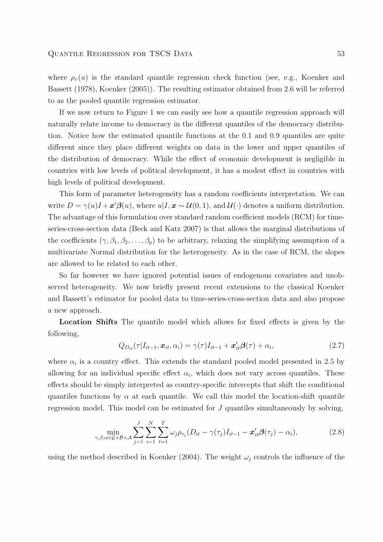
Quantile Regression for TSCS Data 61
in a model with covariates, the estimated coefficients are -0.001 at the τ = 0.1 quantile,
-0.005 at the median and -0.074 at the τ = 0.9 quantile. Once we add country effects the
estimated relationship between income and democracy disappears at all quantiles, with the
exception of the 0.9 quantile. Notice that the mean effect misses important information,
because the effect of income on democracy is not negligible at the upper tail.
Model including
Other Region Year Quantiles
Covariates effects effects 0.10 0.25 0.50 0.75 0.90
Polity measure - Instrumental Variables Set 2
Income Yes No No 0.018 0.000 0.284 0.224 0.125
(0.008) (0.009) (0.007) (0.015) (0.010)
Income Yes Yes No 0.000 0.000 0.000 0.000 0.000
(0.017) (0.022) (0.035) (0.052) (0.043)
Income Yes Yes Yes 0.000 0.000 0.000 0.000 -0.013
(0.086) (0.119) (0.102) (0.122) (0.152)
Polity measure - Instrumental Variables Set 3
Income Yes No No 0.013 0.000 0.178 0.054 0.000
(0.013) (0.016) (0.041) (0.033) (0.014)
Income Yes Yes No 0.072 0.000 0.000 0.000 0.009
(0.012) (0.006) (0.007) (0.011) (0.007)
Income Yes Yes Yes 0.000 0.218 0.000 0.189 0.040
(0.289) (0.442) (0.373) (0.274) (0.512)
Table 4.3: Sensitivity analysis for the instrumental variables.The second set of instruments
includes log of mountainous terrain, geographic latitude, log of air distance to nearest
port; the third set includes the five instrumental variables presented in the appendix. The
first set of instruments presented in Table 4.2 includes trade-weighted world income as in
Acemoglu et. al. (2008). Standard errors in parenthesis.
4.2 Robustness to instrument choice In Table 4.2, we presented the estimation
results for the baseline model after we instrument income with the variable considered in
Acemoglu et al (2008). In Table 4.3, we extend the analysis to consider two additional
sets of instruments. First, we employ geographic variables traditionally associated with
economic development. The IV Set 2 includes mountainous terrain, geographic latitude

62 Alexander, Harding and Lamarche
and the distance to the nearest port. Lastly, we use the IV set 3 corresponding to the
Global economic factors, and constructed as in Section 7.
Basic statistics of the five factor instruments used are presented in Table 3.1. While it
is not necessary nor feasible to interpret the proposed instruments in a concrete economic
setting, it is interesting to note that the chosen principal components have similar statistical
properties across world regions. The first factor appears to be more important for Western
democracies, while the second factor for Sub-saharan African countries. Similarly the fourth
factor appears less important for Eastern Europe and the Soviet Union. This is consistent
with the notion that we are capturing global economic factors acting as sources for the
transmission of international business cycles while still expecting regional variation in their
impact.
In models without regional effects, estimation using the second set of instruments, cor-
responding to the geographic variables, only replicates the inverted U-shaped relationship
as described in the previous section. If we now employ our last set of proposed instru-
ments, we find that the inverted U-shape relationship is also preserved. Once again, the
inverted U-shaped relationship between income and democracy disappears when we include
indicators to account for effects constant over time and common to all countries within a
region. The specifications appear to confirm a negligible effect of income on democracy in
the middle range of the democracy distribution. Thus, after implementing three different
strategies addressing the potential endogeneity of income, we find higher income not to
be an important force for democratization in “hybrid regimes” close to the median of the
democracy distribution and to have almost no effect in non-democratic regimes.
4.3 Additional TSCS data results Using Figure 4.2, we present results obtained
by all the variants of quantile regression methods presented in Section 2 including time-
series-cross-section data approaches. Figure 4.2 (panel (a)) compares the estimated quantile
effects of income on democracy between the quantile regression (QR) estimator correspond-
ing to the pooled model, and the instrumental variable (IV S1-3) estimators. We see a clear
inverted U-shaped relationship between income and the estimated effect, suggesting that
the effect of income varies across the conditional distribution of democracy. The effect of
income is negligible at the tails, but it seem to cause a movement toward democracy at the
center of the conditional distribution. Figure 4.2 (panel (b)) indicates that this conclusion
is incorrect. The inclusion of geographic factors, potentially accounting for omitted variable

Quantile Regression for TSCS Data 63
bias, reduces the effect of income at all quantiles. Most of these income effects obtained
from IV models are dramatically reduced. In the panel (c), we employ fixed effects quantile
regression (FEQR) estimator for a model with a location shift (LS) and a distributional
shift (DS), and fixed effects instrumental variable (IVFE) estimator considering the three
sets of instruments (S1-S3). While the first class of estimator addresses unobserved country
heterogeneity, the second class of methods is designed to address country heterogeneity and
the potential endogeneity of income. Although the results are qualitatively different than
the results presented in the middle panel, they lead to the same conclusion. Income does
not seem to cause a movement toward democracy.
Panel (c) also suggests that allowing the individual effects αi’s to have a distributional
shift does not appear to change the estimated coefficients of income, but does potentially
provide us with more information on the heterogeneous impact of the long run country
specific factors they are designed to capture. In panel (d), we plot the country effects
estimated at different quantiles of the conditional Polity measure distribution. Quantile
country effects, which are allowed to vary over the distribution of the dependent variable,
are estimated at all quantiles measuring the horizontal distances among country’s con-
ditional distributions. Because we estimate a model without intercept and N individual
effects, the lines represent estimated horizontal displacements at each quantile of the con-
ditional distribution of democracy. Therefore, the results on the lower tail suggest that the
conditional distribution of democracy of other (non-western) countries is shifted “down-
ward” by latent variables that are constant over time, possibly associated to historical
factors and institutions. Moreover, the evidence in panel (d) is consistent with the claim
that income is particularly ineffective at “shifting” political outcomes in the lower quantiles
of the democracy distribution.
5 Implications of the Main Results The previous analysis offer two important
implications. First, it suggests that income does not exert a distributional shift on the con-
ditional distribution of democracy. This result is in contrast to the recent work in political
science but which nevertheless appears to emphasize the heterogeneous nature of politi-
cal development at different levels of development. Przeworksi and Limongi (1997) and
Przeworski et. al. (2000) argue that countries often become democratic for reasons which
do not appear to be connected to income, but once they are democratic more prosperous
countries are more likely to remain democratic. Epstein et. al. (2006) highlight the impor-

64 Alexander, Harding and Lamarche
0.0 0.2 0.4 0.6 0.8 1.0
−0.
10.
00.
10.
20.
3(a) Without geographic effects
τ
Inco
me
QRIV S1IV S2IV S3
0.0 0.2 0.4 0.6 0.8 1.0−
0.1
0.0
0.1
0.2
0.3
(b) With geographic effects
τ
Inco
me
QRIV S1IV S2IV S3
0.0 0.2 0.4 0.6 0.8 1.0
−0.
10.
00.
10.
20.
3
(c) With country effects
τ
Inco
me
FEQR (LS)FEQR (DS)IVFE S1IVFE S2IVFE S3
0.0 0.2 0.4 0.6 0.8 1.0
−1.
0−
0.5
0.0
0.5
1.0
(d) Distributional shifts
τ
Cou
ntry
Effe
ct
Figure 4.2: Quantile regression estimates of the effect of income on democracy considering
the full sample of countries. The panels show point estimates obtained by using quantile
regression for the pooled data (QR), instrumental variable with and without fixed effects
(IVFE, IV), and quantile regression with fixed effects assuming that the individual effects
are either location shifts (LS) or distributional shifts (DS). The instrument sets (S1-S3) are
described in Table 3.1.
Quantile Regression for TSCS Data 65
Model including Least Squares Estimation
Other Region Main Models Robustness to IV choice
Covariates effects TSCS Cross-section
(1) (2) (3) (4) (5) (6)
Income Yes No 0.214 0.263 0.263 0.224 0.181 0.162
(0.108) (0.051) (0.052) (0.044) (0.039) (0.044)
Income Yes Yes 0.089 -0.017 -0.165 0.037 0.042 -0.158
(0.131) (0.279) (0.286) (0.155) (0.490) (0.311)
Observations 4735 4640 4640 4640 100 100
Instrument Set 1 Set 4 Set 5 Set 6 Set 4 Set 5
F statistic Yes No 445.3 427.1 403.9 511.8 24.1 19.59
p-value 0.000 0.000 0.000 0.000 0.000 0.000
F statistic Yes Yes 425.6 13.75 16.41 59.48 0.220 1.150
p-value 0.000 0.000 0.000 0.000 0.801 0.321
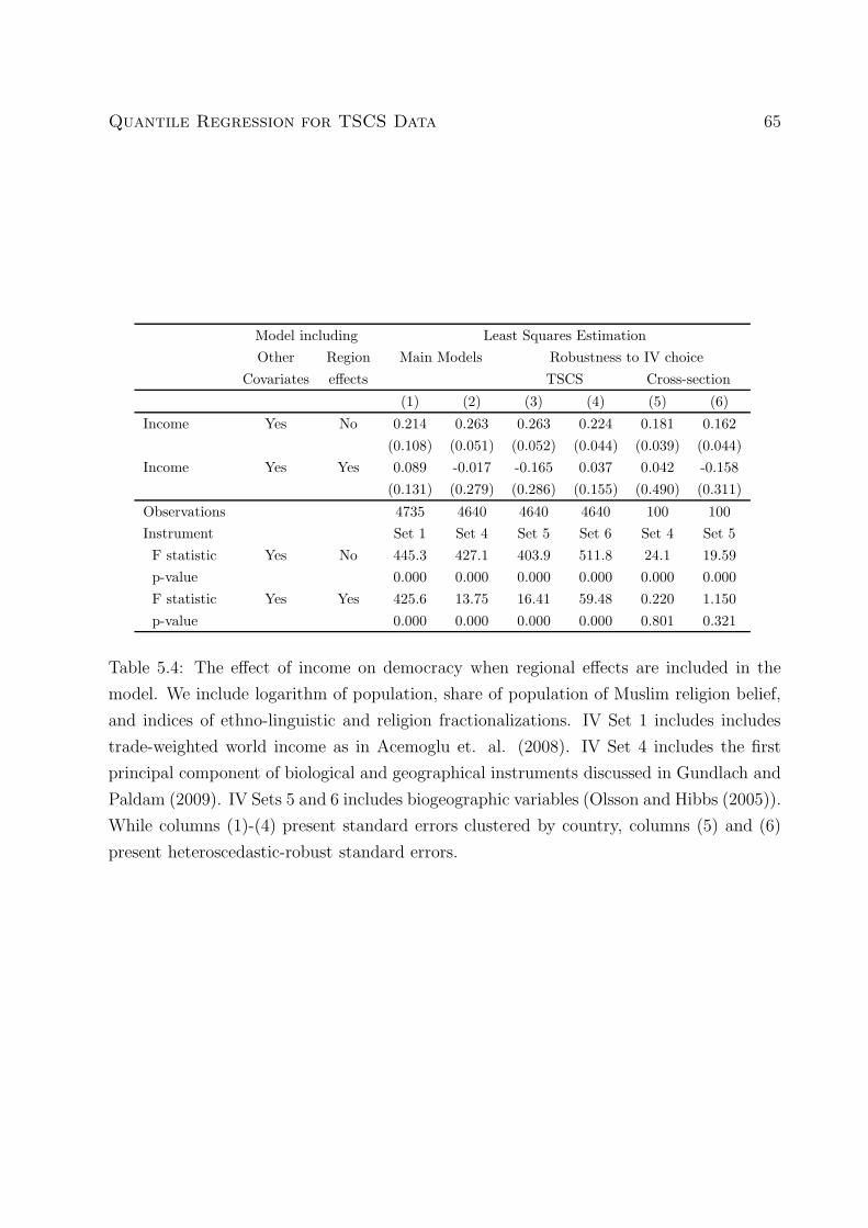
Table 5.4: The effect of income on democracy when regional effects are included in the
model. We include logarithm of population, share of population of Muslim religion belief,
and indices of ethno-linguistic and religion fractionalizations. IV Set 1 includes includes
trade-weighted world income as in Acemoglu et. al. (2008). IV Set 4 includes the first
principal component of biological and geographical instruments discussed in Gundlach and
Paldam (2009). IV Sets 5 and 6 includes biogeographic variables (Olsson and Hibbs (2005)).
While columns (1)-(4) present standard errors clustered by country, columns (5) and (6)
present heteroscedastic-robust standard errors.

66 Alexander, Harding and Lamarche
tance of “partial democracies”, countries with fragile democratic status which tend to be
volatile and highly heterogeneous. These studies appear to point out varying mechanisms
for political development as well as heterogeneous relationship between economic and polit-
ical development at different stages of democratization. Our results however are consistent
with Acemoglu’s et al (2008) conditional mean results, suggesting that income does not
cause movement toward democracy at different quantiles of the conditional distribution of
democracy.
Second, the evidence suggests that it is important to account for omitted variables
associated to income. Przeworski et. al. (2000) find that there is a positive association
between income and democracy, but it tends to disappear when fixed effects are included
in the model. Figure 4.2 suggests that one can address the omitted variable bias simply by
adding indicators for geographic regions, which is potentially important for cross-sectional
studies.
We illustrate this point by extending the empirical evidence to also consider other
conditional mean models recently estimated in the literature. Table 5.4 shows least squares
estimation results of the effect of income on democracy, considering the instrument used in
Acemoglu et al. (2008) and the instruments used in Gundlach and Paldam (2009) (columns
(1) and (2)). Gundlach and Paldam (2009) use the first principal component of biological
instruments and geographic instruments, labeled Set 4 in column (2). Additionally, we
present results considering other instruments. While Set 5 includes plants and animals
as in Olsson and Hibbs (2005), Set 6 includes climate, axis, and latitude as introduced
in Olsson and Hibbs (2005). We report in columns (3) and (4) time-series-cross-section
data results, and for comparison reasons, we report in columns (5) and (6) results for
the year 1991. To avoid biases in terms of precision, we report standard errors clustered
by country in time-series-cross-section data models, and robust standard errors in cross
sectional specifications.
The results of the first model suggest a positive causal effect from income to democracy,
which seem to confirm empirically Lipset’s (1959) thesis. Notice however that the result
is not robust to the inclusion of controls for geographic regions. The effect of income is
reduced and becomes insignificant in all the specifications. The table reveals that the point
estimates are reduced from 0.214 to 0.089 in column (1) and from 0.263 to -0.017 in column
(2). In the case of cross-sectional data, the point estimates are reduced from 0.181 to 0.042
when we consider the instruments proposed by Gundlach and Paldam (2009). This suggests

Quantile Regression for TSCS Data 67
that their results are not robust to a simple variation in the model. While income is not
correlated with democracy in empirical studies using fixed effects, recent studies using
standard instrumental variable methods could address the endogeneity of income and the
omitted variable bias simply by adding indicators for the regions of the world. This strategy
seem to account for omitted variable biases not captured by other control variables, and
leads to what it seems to be a unified result that income does not cause democracy.
6 Conclusion This paper introduces quantile regression as a robust, more descriptive
statistical method in the analysis of TSCS data. It emphasizes the advantages of a method
that allows us to obtain deeper insights into the effect of the regressors on the outcome of
interest by allowing for heterogeneous marginal effects across the conditional outcome dis-
tribution. The paper shows that the method offers the possibility of addressing endogeneity
and different specifications of individual effects. Our analysis has important practical im-
plications for using quantile regression and least squares methods in TSCS data studies
and emphasizes the computational ease with which these more advances methods can be
implemented by the applied researcher.
From a substantive point of view, this paper reexamines the hypothesis that higher
income causes a transition to democracy. We first find that higher income levels have
the strongest effects on political development at intermediate levels of democratization
and almost no effect in countries at the extremes of the distribution of democracy. This
relationship, however, does not survive a number of different identification strategies, dis-
appearing once we account for country specific effects or geographic effects. The evidence
also suggests that country effects become less important as a country develops politically
towards democracy, which could be interpreted as suggesting that institutions are the key
to understand the distance in the political spectrum between authoritarian regimes and
liberal democracies. Country-specific effects that include the complex milieu of institu-
tions, historical legacies and culture entirely may explain why countries have authoritarian
governments.
7 Appendix It is immediately apparent that one of the main problems we face in esti-
mating the basic model 2.1, is that we need to address the issues of reverse causality. Since
the least squares literature offers several standard estimation strategies for the conditional

68 Alexander, Harding and Lamarche
mean model, we focus on the choice of the instrument set and the robustness of the results
to different choices.
Trade-Weighted World Income Instrument. As Robinson (2006) remarks, Ace-
moglu et. al. (2008) are the first ones to propose an instrumental variable approach to the
identification of the causal effect of income on democracy. Acemoglu et. al. (2008) use
two different instruments for income in their linear specification. The second instrument
corresponds to the trade-weighted world income. Let ωij denote the trade share between
country i and j in the GDP of country i between 1980-1989. Then we can write the income
of country i at time t − 1 as,
Iit−1 = ζ
N∑
j=1,j 6=i
ωijIjt−1 + ǫit−1 (7.1)
where income is measured as log of total income and ǫ is a Gaussian error term. Acemoglu
et. al. (2008) suggest the use of the weighted sum of world income for each country, Iit−1, as
an instrument. Notice that the weights are not estimated but correspond to the actual trade
weights. This instrument may be problematic if income in country j, Ijt−1, is correlated
with democracy in country j which itself is then correlated to democracy in country i.
Furthermore, the trade weights, ωij may be correlated with the relative democracy scores
of countries i and j.
Geographic Instruments. While the political science literature on democratization
seems to have ignored the potential endogeneity of income in this specification, economics
has traditionally stressed differences in geography as a potential determinant of economic
development (Acemoglu, Johnson and Robinson, 2001, Sachs and Malaney (2002), Nunn
and Puga (2009); see, e.g., Acemoglu, Johnson, and Robinson for a detailed introduction to
the geography hypothesis). We will use the log of mountainous terrain, geographic latitude
and the log of air distance to the nearest port as instruments.
Global Economic Factors. The world income instrument described above has an
appealing interpretation since it is designed to capture the intuition that business cycles
are to some extent correlated with events in world markets. A statistical factor model can
be employed to recover a set of orthogonal factors that can act as international sources of
domestic economic fluctuations (Kose et. al., 2003). These global factors drive, to some
extent, the domestic business cycle independently of the political regime of a country. We
write,
It−1 = ΛFt−1 + Ut−1, (7.2)

Quantile Regression for TSCS Data 69
where It−1 is the observed N dimensional vector of log GDP, Ft−1 is a p-dimensional vector
of global factors and Ut−1 is a vector of idiosyncratic errors. The coefficient matrix Λ is a
matrix of individual specific weights (factor loadings). Since only log GDP is observed we
need to use a statistical procedure such as Principal Components Analysis (PCA) applied
to the covariance matrix Σ = (1/T )It−1I′t−1
to recover the latent factors Ft−1.
By construction, this method separates the commonalities Ft−1 from the idiosyncratic
shocks Ut−1. In order to further exclude the possibility that the political regime affects the
global factors through its effect on income, we construct different values of the instruments
for each country by excluding the country from the analysis. Thus, the instruments for
country j correspond to the global factors estimated from the matrix of GDP measures for
all the countries in the world except country j.
Bio-Geographic and Climate Diversity Instruments. The economic literature has
recently explored the use of a novel set of biogeography variables, which could be associated
to the very long run determinants of development (Hibbs and Olsson (2004), Olsson and
Hibbs (2005), and Gundlach and Paldam (2009)). The premise is that these variables
represent exogenous sources of variation, because they are determined in prehistory. The
instrumental variable set considered includes animals (number of big mammals in parts of
the world in prehistory) and plants (number of annual perennial grasses in regions of the
world in prehistory). An additional instrument set that we will explore includes climate,
latitude, and axis (relative east-west orientation of a country). These variables were taken
from Olsson and Hibbs (2005). Following Gundlach and Paldam (2009), we use them to
create the first principal component of biological and geographical instruments.
Acknowledgement.
We are grateful to Tim Hyde for excellent research assistance. We are grateful to
Robert Bates, Victor Chernozhukov, Jorge Dominguez, Dawn Brancati, Margarita Estavez-
Abe, Kevin Grier, Yoshiko Herrera, Nahomi Ichino, Torben Iversen, Gary King, Roderick
MacFarquhar, Thomas Remington, James Robinson and seminar participants at Harvard,
Stanford, and the 2009 AEA meeting for useful comments, and to Daron Acemoglu, James
Robinson, Simon Johnson and Pierre Yared for sharing their historical data.
References

70 Alexander, Harding and Lamarche
[1] D. Acemoglu, S. Johnson, and J. A. Robinson. The colonial origins of comparative
development: An empirical investigation. American Economic Review, 91:1369–1401,
2001.
[2] D. Acemoglu, S. Johnson, and J. A. Robinson. Reversal of fortune: Geography and
institutions in the making of the modern world income distribution. Quarterly Journal
of Economics, 118:1231–1294, 2002.
[3] D. Acemoglu, S. Johnson, J. A. Robinson, and P. Yared. Income and democracy.
American Economic Review, 98(3):808–842, 2008.
[4] R. J. Barro. The determinants of democracy. Journal of Political Economy, 107:S158–
S183, 1999.
[5] N. Beck and J. Katz. Random coefficient models for time-series-cross-section data:
Monte carlo experiments. Political Analysis, 15:182–195, 2007.
[6] V. Chernozhukov and C. Hansen. Instrumental variable quantile regression: A robust
inference approach. Journal of Econometrics, 142(1):379–398, 2008.
[7] D. L. Epstein, R. H. Bates, J. Gladstone, I. Kristensen, and S. O’Halloran. Democratic
transitions. American Journal of Political Science, 50(3):551–569, 2006.
[8] J. Fearon and D. Laitin. Ethnicity, insurgency, and civil war. American Political
Science Review, 97(1):75–90, 2003.
[9] S. Firpo, N. M. Fortin, and T. Lemieux. Unconditional quantile regressions. Econo-
metrica, 77:953–973, 2009.
[10] E. Gundlach and M. Paldam. A farewell to critical junctures: Sorting out long-run
causality of income and democracy. European Journal of Political Economy, 25:340–
354, 2009.
[11] P. A. Hall and D. Soskice, editors. Varieties of Capitalism: The Institutional Founda-
tions of Comparative Advantage. Oxford University Press, Oxford, 2001.

Quantile Regression for TSCS Data 71
[12] M. Harding and C. Lamarche. A quantile regression approach for estimating panel
data models using instrumental variables. Economics Letters, 104:133–135, 2009.
[13] D. A. Hibbs Jr. and O. Olsson. Geography, biogeography, and why some countries are
rich and others are poor. Proceedings of the National Academy of Sciences (PNAS),
101:3715–3740, 2004.
[14] K. Jaggers and T. R. Gurr. Tracking democracy’s third wave with the polity iii data.
Journal of Peace Research, 32:469–482, 1995.
[15] R. Koenker. Quantile regression for longitudinal data. Journal of Multivariate Anal-
ysis, 91:74–89, 2004.
[16] R. Koenker. Quantile Regression. Cambridge University Press, 2005.
[17] R. Koenker and G. Bassett. Regression quantiles. Econometrica, 46:33–50, 1978.
[18] M. Kose, C. Otrok, and C. Whiteman. International business cycles: World, region
and country-specific factors. American Economic Review, 93(4):1216–1239, 2003.
[19] A. Lijphart. Patterns of democracy : government forms and performance in thirty-six
countries. Yale University Press, New Haven, 1999.
[20] S. M. Lipset. Some social requisites of democracy: Economic development and political
legitimac. American Political Science Review, 53:69–105, 1959.
[21] S. M. Lipset. Political Man: The Social Bases of Politics. Anchor Books, New York,
1963.
[22] N. Nuamah. Pooling cross section and time series data. The Statistician, 35:345–351,
1986.
[23] N. Nunn and D. Purga. Ruggedness: The blessing of bad geography in africa. NBER
Working Paper 14918, 2009.
[24] O. Olsson and D. A. Hibbs Jr. Biogeography and long-run economic development.
European Economic Review, 49:909–938, 2005.
72 Alexander, Harding and Lamarche
[25] A. Przeworski, J. A. Cheibub, M. E. Alvarez, and F. Limongi. Democracy and Devel-
opment: Political Institutions and Well-Being in the World, 1950-1990. Cambridge
University Press, Cambridge, 2000.
[26] A. Przeworski and F. Limongi. Modernization: Theory and facts. World Politics,
49:155–183, 1997.
[27] J. A. Robinson. Economic development and democracy. Annual Reviews of Political
Science, 9:503–527, 2006.
[28] J. Sachs and P. Malaney. The economic and social burden of malaria. Nature, pages
680–685, 2002.