Embed Size (px)
Citation preview

ISSN: 1439-2305
Number 210 – January 2016
IS AID FOR TRADE EFFECTIVE?
A PANEL QUANTILE REGRESSION
APPROACH
Inmaculada Martínez-Zarzoso
Felicitas Nowak-Lehmann
Kai Rehwald
1
Is Aid for Trade Effective? A Panel Quantile
Regression Approach by
Inmaculada Martínez-Zarzoso*1, University of Goettingen and University Jaume I
Felicitas Nowak-Lehmann D.*, University of Goettingen
Kai Rehwald**, University of Aarhus
Abstract
This paper investigates whether Aid for Trade (AfT) leads to greater exports in recipient countries. Using panel
data and panel quantile regression techniques, our results suggest that total AfT disbursements promote the export
of goods and services, but is limited primarily to exporters above the .35 quantile of the conditional distribution of
exports. When disaggregating by type of AfT, we find that aid to improve trade policy and regulation is not
associated with higher exports. Aid to build productive capacity is effective for almost all quantiles of the export
distribution but the 10th, with the effect being stronger at the higher tails of the conditional distribution. Aid used to
build infrastructure is found to affect exports only at the 0.10 quantile. In contrast, aid disbursed for general budget
support (an untargeted type of aid) is not associated with greater export levels irrespective of the quantile.
Key Words: development aid; North-South trade; aid for trade; panel data; aid effectiveness JEL Codes: F14, F35, O10, C22, C23
* Department of Economics, University of Goettingen, Platz der Goettinger Sieben 3, 37073, Goettingen, Germany. Tel: 0049551397487; Fax: 0049551398173; e-mail: [email protected] (corresponding author: Felicitas Nowak-Lehmann D.). **Department of Economics, University of Aarhus, Nordre Ringgade 1DK-8000 Aarhus.
1 The authors would like to thank the participants of the research seminar held at the University of Bochum, the
International Economics Workshop held in Goettingen and the DEGIT Conference in Geneva for their helpful comments and suggestions, which have been incorporated into the paper. Inmaculada Martinez-Zarzoso would like
to acknowledge the funding received from the Spanish Ministry of Economy and Competitiveness (project
ECO2014-58991-C3-2-R) and Universitat Jaume I (P1- 1B2013-06).
2
Is Aid for Trade Effective? A Panel Quantile
Regression Approach
1. Introduction
Aid for Trade (AfT) became a buzz word in aid policy just a few years ago, but is far from being
a new concept in development policy (Evenett, 2009). Dating back to the 1986-1994 Uruguay
Round of the Multilateral Trade Negotiations (MTN), developing countries began demanding
financial compensation for concessions made in trade liberalization negotiations2 as well as an
increase in development aid to help facilitate integration into the world trading system. Aid that
serves the latter objective is usually considered AfT. As trade liberalization negotiations became
more problematic in the late 1990s and early 2000s given that the “easier” concessions had
already been made on both sides (developed and developing countries), WTO members
separated the AfT initiative from the Doha Round negotiations and established a WTO ‘Aid for
Trade Task Force’ in July 2006. According to the WTO AfT task force, the objectives of the
AfT initiative are to promote growth and development through trade across developing
countries, especially in the least developed countries (LDCs); and through their integration into
the world trading system. This is achieved through a more trade-oriented infrastructure, an
improved production capacity, and by supporting negotiations concerning trade policy
regulation and trade liberalization. As AfT is considered an important instrument for
development aid, the European Union, the United States, and Japan made non-binding
concessions to increase AfT disbursements. However, the means for AfT have not increased
substantially (García, 2008; Luke, 2009; Huchet-Bourdon et al., 2009; Karingi, 2009). In the
period from 2002 to 2009, AfT ranged from only 20 to 30% of total official development
assistance (ODA). Although AfT did increase during this period, other types of aid increased
2 Compensation payments for trade liberalization were the original type of AfT.
3
even faster (Karingi, 2009). In Africa, the AfT share shrank from 29% in 2002 to 21% in 2006.
In real terms, 2010 AfT commitments were extremely high at US$ 48 billion, falling by 14% to
US$ 41 billion in 2011. Meanwhile, AfT disbursements were less affected by the 2011 decline
in ODA; disbursements declined by only 3.7% to US$ 33.5 billion.
In recent years, development economists have become more aware of the challenges of
overall ODA in promoting trade and economic growth in developing countries (Doucouliagos
and Paldam, 2008; Rajan and Subramanian, 2008; Nowak-Lehmann D. et al., 2012; Nowak-
Lehmann D. et al., 2013). Many existing studies find that ODA is ineffective, in that it produces
no significant impact on per capita income and recipient-country exports. However, these
studies fail to differentiate3 between the different types of aid, such as: AfT, technical assistance,
humanitarian aid, sector-specific aid, etc. This could explain why the authors of this paper were
unable to find a positive impact of aid.
Given the objectives of AfT, the question remains: Is AfT effective? In particular, we
investigate whether AfT is associated with higher exports of goods and services. To the best of
our knowledge, existing literature on AfT-effectiveness is scarce, as pointed out by Vijil and
Wagner (2012), and most of the work consists of case studies at the country level. The main
contribution of this paper to existing literature is its methodological approach using panel-
quantile regression techniques, which allows us to investigate whether AfT has different effects
along the conditional distribution of exports while controlling for unobserved country
heterogeneity. More specifically, we study whether AfT benefits countries that have certain
export disadvantages and therefore have a weaker export capacity. Being able to answer this
question is extremely relevant as it would facilitate the better targeting of AfT funds based on
the export capacity and AfT efficiency of the recipient countries.
The main results show that total AfT disbursements and its sub-categories do not always
promote exports of goods and services with respect to average size exporters over the period
3 Rajan and Subramanian (2009) investigated different types of aid but could not establish significant differences between these types.
4
from 2002 to 2011. We find that exporters only benefit at certain quantiles of the conditional
distribution of exports and from certain AfT categories. In particular, aid used to improve trade
policy and trade regulation does not affect exports, whereas aid to build production capacity does
with relatively high impacts for the 0.35, 0.50, 0.75 and 0.90 quantiles of the export distribution.
Aid used to build economic infrastructure also positively affects exports, but only for the 0.1
quantile of the distribution. This is good news as it shows that aid is effective for the more
disadvantaged countries that have a greater need for economic infrastructure. Conversely, aid
disbursed to general budget support (a control variable), which is considered to be an untargeted
component of development aid, is not associated with higher exports. It even has a negative
contribution on export expansion. This holds true irrespective of the quantile.
The rest of the paper is structured as follows. Section 2 presents the empirical model that
we use to analyse AfT effectiveness. Section 3 discusses the variables, data and descriptive
statistics. Regression results are presented and evaluated in Section 4, and Section 5 contains the
concluding remarks.
2. Literature review
The effectiveness of AfT is currently assessed using one of two approaches. The first approach
examines whether AfT reduces the cost of trading or other impediments to trade. Calì and te
Velde (2011) and Busse et al. (2011) find that aid for infrastructure and aid for trade facilitation
lower transport costs and thus promote exports. The second approach, which is used in this
paper, analyses whether AfT is directly associated with improved export performance (measured
by the value of exports of goods and services). Earlier studies found a positive relationship
between AfT or at least some of its components, and trade-related outcomes. Among these
studies, Bearce et al. (2013) find that AfT issued by the US government has a positive effect on
the recipient country's export performance; Vijil and Wagner (2012) suggest that aid to trade-
5
related infrastructure4, as part of overall AfT, has a positive impact on exports as a ratio to GDP;
and Calì and te Velde (2011) find that AfT has an overall positive and significant effect on
exports, driven by AfT for economic infrastructure which has the additional effect of lowering
trade costs. Both Vijil and Wagner (2012) and Calì and te Velde (2011) emphasize that the
infrastructure channel is the main driver of AfT effectiveness. However, Helble, Mann and
Wilson (2012) find that aid for trade policy and regulations (another AfT category) is also
effective. The authors find that a 1% increase in aid for trade policy and regulation increases
trade value by around US$ 347 million. Hühne et al. (2014) investigated the impact of AfT on
both donor and recipient countries. For recipient countries, they find total AfT and its
components (infrastructure-related aid, aid for building and improving productive capacity and
aid for trade policy and regulation) are all effective. However, when breaking the sample down
into groups by income and region, the results become mixed. AfT tends to favour the richer
developing countries and countries in Asia and Latin America. None of the revised studies
examine the effect of AfT along the distribution of exports, which is the central focus of this
paper.
3. Empirical Model
3.1 Baseline model
As a framework for analysis, we estimate the model proposed by Calì and te Velde (2011) using
the latest AfT data. The authors identify the types of AfT that can help address governance
failures in developing countries by associating the main aid categories, as classified by OECD
statistics, with a number of goals that are related to trade performance, e.g. aid for trade policy
and regulations should improve weak institutions. They also refer to the complexity of the
economic channels through which AfT affects export performance. This includes Dutch-disease
effects as well as direct and indirect competitiveness effects. The authors claim, however, that
causality is less complex than for the aid-economic growth link.
4 Throughout this paper, we refer to this type of aid as “aid for economic infrastructure”.
6
iti
l
ltl
h
xhithititititit
D
AfTCPIGEMPPOPExp
)ln()ln()ln()ln( 43210
iti
l
ltl
k
kitkit DXExp 0
The empirical model used to analyse AfT effectiveness is an export demand equation
augmented with aid for trade variables and is given by:
(1)
where Expit denotes exports of country i in year t, Xkit are explanatory variables (AfT and a
number of control variables), Dlt are time dummies, i denotes country-specific unobserved
heterogeneity, and Ɛit is the error term. The unobserved effects, i, are country-specific and
time-invariant and represents unobserved country heterogeneity that can be treated as fixed or
random to fit the model. The baseline is the following static unobserved effects model:
(2)
where ln denotes natural logs. We regress exports (Expit) on lagged proxies for AfT (AfThit-x)
while controlling for population size (POPit), market potential (MPit), government effectiveness
(GEit) and the consumer price index (CPIit). Time dummies (Dlt) and the country-unobserved
effects (i) are also included.
Model (2) is a generalized version of the model used by Calì and te Velde (2011: 730).
There are two main differences. First, we use exports of goods and services as a dependent
variable, whereas the authors use merchandise exports. Second, the authors use only two AfT
categories, while we use three.
The reasons for our choice of dependent and explanatory variables are as follow. First,
there is no reason to limit the scope of analysis to merchandise exports. Service exports, for
example, could also be fostered by AfT. AfT is not aimed exclusively at merchandise exports
7
nor would we expect the export performance of service sectors to be unaffected by AfT.5
Consequently, we use exports of goods and services as the dependent variable in our
regressions. Second, when analysing the effect of AfT on exports, a specific measure of AfT
must be selected (i.e. selecting which AfT categories to include in the estimations). Calì and te
Velde (2011) only use aid disbursed for economic infrastructure (CRS category 200) and aid
disbursed to production capacity (CRS category 300). Unlike their study, we make use of three
AfT proxies: aid to trade policies and regulation (TPR), aid to economic infrastructure (EI) and
aid to building production capacity (BPC). Our choice of AfT proxies allows us to be more
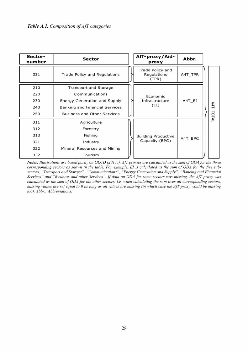
specific and its components are listed in Table A.1.
To put our results into perspective, we compare the impact of AfT with the impact of aid
to general budget support (GBS), which is non-targeted and might be used by recipients for trade
development but it is not included in total AfT. Lastly, we experiment with three alternative
measures of market potential. The concept of market potential dates back to Harris (1954). Calì
and te Velde (2011: 730) calculate the market potential6 of country i at time t as the sum of the
(inverse) bilateral distance (dij) weighted GDPs of all other countries, i.e.
(
3)
5 Aid for economic infrastructure (which is part of overall AfT and is used to build roads and ports, among other things), may have an impact on the tourism sector (which, especially in developing countries, may account for a substantial portion of total exports). 6 Note that the market potential of country i at time t is calculated as the sum of the (inverse) bilateral distance weighted GDPs of all other countries and not only of all countries for which we analyse the effect of AfT on exports - which are, of course, mostly developing countries.
j ij
jt
itd
GDPMP
8
Generally speaking, as Overman, Redding and Venables (2001:12) explain, market potentials
can also be computed as:
(4)
where serves as a “distance weighting parameter”. By varying the size of the distance
weighting parameter, we obtain different measures of market potential:
(5)
Note that we would expect greater market potential to be (ceteris paribus) associated
with higher exports.
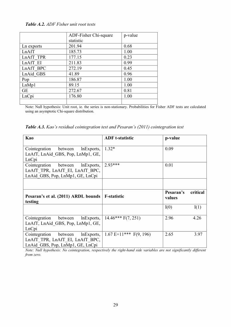
Before looking at the impact of AfT and its sub-categories on exports in different
quantiles of the export distribution, we want to make sure that we do not run spurious
regressions. To this end we test the time-series properties of our series (see Appendix Table A.2)
and test for cointegration by means of Kao’s and Pesaran’s et al. (2011)7 cointegration test (see
Appendix Table A.3). We find all series to be non-stationary (I(1)) and cointegrated, i.e. they
have a systematic relationship in the period under study.
Having found cointegration, we estimate an OLS regression with regional dummies, a
fixed-effects model and a dynamic panel-data GMM model, which includes lagged exports as
right-hand-side variable and controls for endogeneity of lagged exports and (potentially) AfT.
The above-mentioned models are conditional mean regression models and yield our baseline
results. The dynamic panel data model is given by:
7 Pesaran’s cointegration test, which is based on an unrestricted Error Correction Model (ARDL) supports the finding of cointegration.
ij
j
jtit dGDPMP
j ij
jt
itd
GDPMPMP )1(1
j ij
jt
itd
GDPMPMP )5.0(2
j ij
jt
itd
GDPMPMP
2)2(3
9
D ln(Expit )= b0 +b1DPOPit +b2D ln(MPit )+b3DGEit +b4D ln(CPI it )+ dhD ln(AfThith=1
H )+
lll=1
L DDlt +g D ln(Expi,t-1)+uit (6)
where h is the number of different AfT types, l is the number of time fixed effects, and
stand for the first difference of the variables.
3.2 Quantile regression model
A novel specification considered in this paper is the application of a quantile regression for
panel data, which was recently proposed by Canay (2011). He suggests a simple transformation
to account for fixed effects, assuming that these effects are location shifters. The author
develops a two-step approach that consists of estimating country fixed effects (FE) using a
within-FE model as a first step. As a second step, the consistently estimated FE are used to
demean the dependent variable (log of exports) and this transformed variable is taken as a
dependent variable in a quantile regression.
The model estimated in the first step is given by equation (2) above. Then, the estimated
αi are used to transform ln (Expit) into
The quantile regression is estimated as:
(7)
5. Data, variables and main results
5.1. Variables, Data and Descriptive Statistics
In this section, we discuss the data and present variable descriptions and sources, as well as
descriptive statistics. The panel dataset used in our empirical analysis covers the period from
T
T
n
i
itit XXnT1 1
1 )~
()(minarg)(ˆ
iititEXPX ̂)ln(
~
10
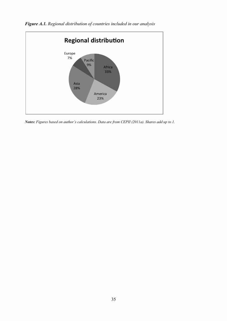
2000 to 2011 and comprises 162 countries (see Table A.4 in the Appendix).8 Figure A.1 shows
the regional distribution. It is worth noting that 19% of the countries are landlocked. Limited
data availability influenced the time and country dimensions of the panel. In particular, data
coverage on AfT for the years before 2000 is incomplete.
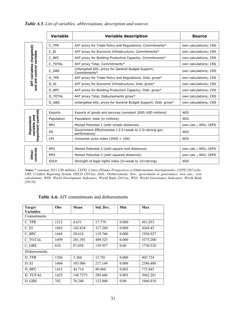
Table A.5 presents a description of the variables used in the analysis, the corresponding
abbreviations, and the sources of the data. Data on AfT —our key explanatory variable— stems
from the Creditor Reporting System (CRS) (OECD, 2013a).9 According to the OECD (2013b),
“[t]he objective of the CRS Aid Activity database is to provide (…) data that enables analysis on
where aid goes, what purposes it serves and what policies it aims to implement (…).” Data on
commitments and disbursements of official development assistance (ODA) is available by
sector, policy objective, type of aid, and purpose code (see Table A.6). Data on disbursement
serve our purpose better as they capture the amounts of aid received by the developing countries
under examination. Using ODA data by sector, we calculated AfT proxies as can be seen in
Table A.1. The OECD identifies five categories of AfT: (1) technical assistance for trade policy
and regulations (e.g. helping countries develop trade strategies, negotiating trade agreements
and implementing their outcomes); (2) trade-related infrastructure (e.g. building roads, ports and
telecommunication networks to connect domestic markets to the global economy); (3)
productive capacity building, including trade development (e.g. providing support to the private
sector to exploit their comparative advantages and diversify their exports); (4) trade related
adjustments (e.g. helping developing countries finance the costs associated with trade
liberalization, such as tariff reductions, preference erosion, or declining terms of trade) and (5)
other trade-related needs, identified as trade-related development priorities in partner countries’
8 While data on AfT is available for 179 countries, there are only 168 countries where data is available for both AfT and exports, our dependent variable. For 6 of these 168 countries, we are unable to calculate market potentials —an important control variable— because data on bilateral distances is missing. We confine the analysis ex ante to those 162 countries for which data on exports, AfT and bilateral distances (market potentials) are available (which does not mean that the data for these 162 countries is complete).
9The CRS database is maintained by the Development Assistance Committee (DAC), which is part of the OECD’s Development Co-operation Directorate (DCD).
11
national development strategies (OECD, 2014). For reasons of data availability, analysis is
limited to the first three categories of AfT.
Data on the export of goods and services (in constant 2005 US$) is from the World
Bank’s World Development Indicators (WDI) database (World Bank, 2013a). From the same
database, we obtained data on Population (in millions) and data on the CPI (with 2005 as the
base year). Data on GDP (in constant 2005 US$), which is needed in order to calculate market
potentials, also comes from the WDI database. Data on bilateral distances —which is needed in
order to calculate market potentials— is taken from CEPII (2013a/b). Data on government
effectiveness (GE) comes from the Worldwide Governance Indicators (WGI) project (World
Bank, 2013b). GE indicates the strength of governance performance. Finally, data on the
strength of legal rights index (SOLR), which “measures the degree to which (...) laws protect the
rights of borrowers and lenders and thus facilitate lending” (World Bank, 2013a), comes from
the WDI database (World Bank, 2013a). The SOLR dataset is not part of our baseline model, but
is used as an alternative to the government effectiveness (GE) index in certain regressions.
Table 1 contains summary statistics of the main variables used in the empirical analysis.
The first part of Table 1 contains summary statistics for the AfT proxies. Proxies for “total” AfT
disbursements (D_TOTAL) are calculated as the sum of the 3 sub-categories of AfT considered.
Table 1: Summary statistics for the AfT-proxies, dependent variable and controls
Target
Variables
Obs Mean Std. Dev. Min Max
Disbursements of AfT
D_TPR 1204 3.360 15.781 0.000 403.724
D_EI 1391 84.549 185.843 .003 2107.355
D_BPC 1421 63.534 114.457 .0031 1179.496
D_TOTAL 1425 148.727 288.606 0.003 3042.281
D_GBS 742 70.240 122.008 0.00 1066.810
Dependent
Variable
Exports 1228 29051.210 108752.000 15.785 1677840
Control
Variables
Population 1788 35.552 142.991 0.009 1344.130
MP1 1728 7907.086 3447.210 3291.178 24758.810

12
GE 1628 -0.464 0.679 -2.454 1.590
CPI 1562 296.858 7418.968 0.288 293318
MP2 1728 558266.1 103877 354308.8 966380.7
MP3 1728 4.273 8.793 0.329 93.052
SOLR 1075 4.805 2.342 0 10
Notes: D_TOTAL is calculated as the sum of D_TPR, D_EI and, D_BPC. When data on some of the three
components was missing, D_TOTAL was calculated as the sum of the others. D_TOTAL values are in constant
2011 US$ millions. Exports = exports of goods and services (constant 2005 US$ millions). Population = total
population (in millions). MP1 = market potential (with simple distances). GE = government effectiveness (-2.5 =
weak to 2.5 = strong government performance). CPI = consumer price index (2005 = 100). MP2/3 = market
potential 2/3 (with square root/squared distances). SOLR = strength of legal rights index (0 = weak to 10 =
strong).
Below, we discuss the AfT-proxies in detail. First, note that the number of observations
for AfT commitments is significantly higher than that for AfT disbursements (see Table A.6).
This is primarily due to the fact that data on disbursements is entirely missing prior to 2002 (in
our case, for 2000 and for 2001).
Second, the average size of AfT commitments and disbursements is notable (see Table
A3). The mean value of AfT commitments for economic infrastructure (C_EI), which is the
average value per country and year, is about US$ 84.5 million. The fact that AfT is quite
sizeable can best be seen when expressed relative to GDP. The ratio of the sum of all AfT
proxies to GDP has a mean value of 2.7% for commitments and 1.5% for disbursements. Third,
AfT commitments tend to be larger and more volatile than AfT disbursements. As can be seen in
Table A.6, mean commitments are strikingly larger than mean disbursements. The correlation
coefficient between total commitments (C_TOTAL) and total disbursements (D_TOTAL) is
about 81%.
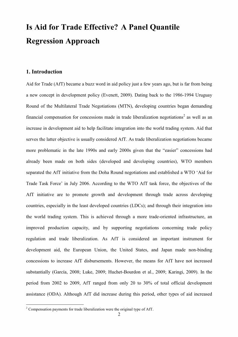
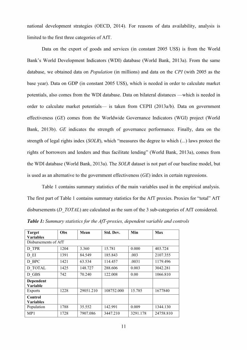
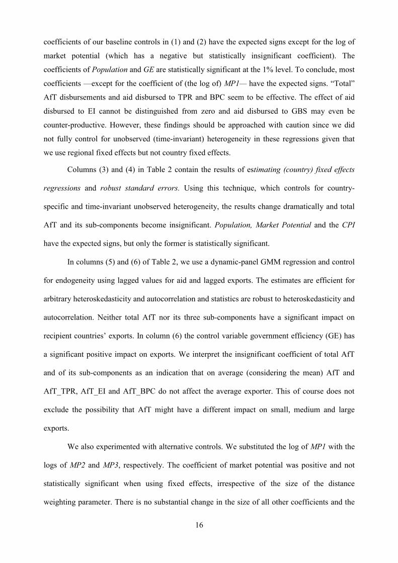
Figure 1 shows a Kernel density function for D_TOTAL. The figure indicates that the
estimated distribution is skewed to the right with most countries receiving relatively little AfT,
with just a few receiving significantly more.10 This fact is also illustrated in Table A.7, which
shows the percentiles for the distribution of D_TOTAL. While the median value of total AfT
disbursements is smaller than US$ 32 million, the 99th percentile is 50 times as large.
Figure 1. Kernel density estimate for total AfT disbursements
10 That “[AfT] (...) is relatively concentrated” is also discussed in OECD/WTO (2011: 14).
13
0
.001
.002
.003
.004
0 500 1000 1500 2000
A4T proxy Total; Disbursements gross (constant 2009 US$ millions)
Source: Own illustration based on own calculations. Data: OECD (2013a). Notes: Kernel = Epanechnikov;
bandwidth = 53.3482.
The second part of Table 1 contains the summary statistics of the dependent and control
variables. It is worth noting here that the CPI (base year: 2005) ranges between 0.288 and
293318. The outliers belong to Zimbabwe, which recently experienced a period of
hyperinflation (see, e.g., Hanke, 2008). The outliers inflate the standard deviation and the mean,
and are therefore eliminated from the final regression. When excluding the observations for
Zimbabwe, the mean (standard deviation) of the CPI drops from over 300 (7,800) to around 100
(25). The CPI is seen as a measure of price competitiveness and replaces the real exchange rate
which has many missing data points (see Calì and te Velde, 2011). We expect an increase in
consumer prices to hinder price competitiveness in the recipient country and to have a negative
sign.
After having presented the empirical model in Section 2; and data and descriptive
statistics in this section, in the following section we discuss the results of the regression
analysis.
0
.00
2.0
04
.00
6
0 1000 2000 3000AfT Total Disb.gross (cons. 2011 USD M)
kernel = epanechnikov, bandwidth = 21.9840
Kernel density estimate
14
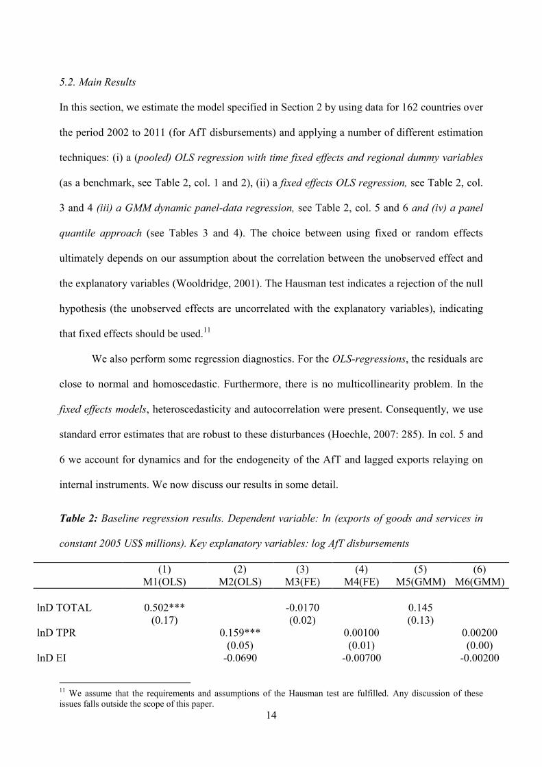
5.2. Main Results
In this section, we estimate the model specified in Section 2 by using data for 162 countries over
the period 2002 to 2011 (for AfT disbursements) and applying a number of different estimation
techniques: (i) a (pooled) OLS regression with time fixed effects and regional dummy variables
(as a benchmark, see Table 2, col. 1 and 2), (ii) a fixed effects OLS regression, see Table 2, col.
3 and 4 (iii) a GMM dynamic panel-data regression, see Table 2, col. 5 and 6 and (iv) a panel
quantile approach (see Tables 3 and 4). The choice between using fixed or random effects
ultimately depends on our assumption about the correlation between the unobserved effect and
the explanatory variables (Wooldridge, 2001). The Hausman test indicates a rejection of the null
hypothesis (the unobserved effects are uncorrelated with the explanatory variables), indicating
that fixed effects should be used.11
We also perform some regression diagnostics. For the OLS-regressions, the residuals are
close to normal and homoscedastic. Furthermore, there is no multicollinearity problem. In the
fixed effects models, heteroscedasticity and autocorrelation were present. Consequently, we use
standard error estimates that are robust to these disturbances (Hoechle, 2007: 285). In col. 5 and
6 we account for dynamics and for the endogeneity of the AfT and lagged exports relaying on
internal instruments. We now discuss our results in some detail.
Table 2: Baseline regression results. Dependent variable: ln (exports of goods and services in
constant 2005 US$ millions). Key explanatory variables: log AfT disbursements
(1) (2) (3) (4) (5) (6) M1(OLS) M2(OLS) M3(FE) M4(FE) M5(GMM) M6(GMM)
lnD TOTAL 0.502*** -0.0170 0.145 (0.17) (0.02) (0.13) lnD TPR 0.159*** 0.00100 0.00200 (0.05) (0.01) (0.00) lnD EI -0.0690 -0.00700 -0.00200
11 We assume that the requirements and assumptions of the Hausman test are fulfilled. Any discussion of these issues falls outside the scope of this paper.
15
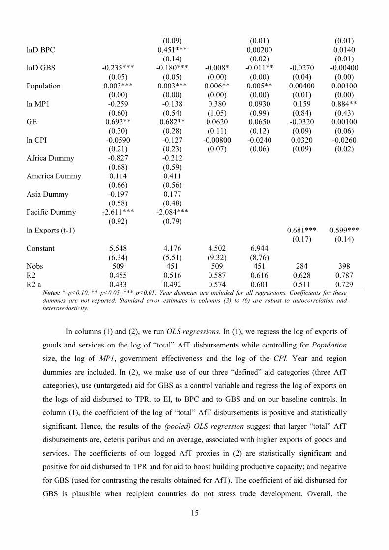
(0.09) (0.01) (0.01) lnD BPC 0.451*** 0.00200 0.0140 (0.14) (0.02) (0.01) lnD GBS -0.235*** -0.180*** -0.008* -0.011** -0.0270 -0.00400 (0.05) (0.05) (0.00) (0.00) (0.04) (0.00) Population 0.003*** 0.003*** 0.006** 0.005** 0.00400 0.00100 (0.00) (0.00) (0.00) (0.00) (0.01) (0.00) ln MP1 -0.259 -0.138 0.380 0.0930 0.159 0.884** (0.60) (0.54) (1.05) (0.99) (0.84) (0.43) GE 0.692** 0.682** 0.0620 0.0650 -0.0320 0.00100 (0.30) (0.28) (0.11) (0.12) (0.09) (0.06) ln CPI -0.0590 -0.127 -0.00800 -0.0240 0.0320 -0.0260 (0.21) (0.23) (0.07) (0.06) (0.09) (0.02) Africa Dummy -0.827 -0.212 (0.68) (0.59) America Dummy 0.114 0.411 (0.66) (0.56) Asia Dummy -0.197 0.177 (0.58) (0.48) Pacific Dummy -2.611*** -2.084*** (0.92) (0.79) ln Exports (t-1) 0.681*** 0.599*** (0.17) (0.14) Constant 5.548 4.176 4.502 6.944 (6.34) (5.51) (9.32) (8.76) Nobs 509 451 509 451 284 398 R2 0.455 0.516 0.587 0.616 0.628 0.787 R2 a 0.433 0.492 0.574 0.601 0.511 0.729
Notes: * p<0.10, ** p<0.05, *** p<0.01. Year dummies are included for all regressions. Coefficients for these
dummies are not reported. Standard error estimates in columns (3) to (6) are robust to autocorrelation and
heterosedasticity.
In columns (1) and (2), we run OLS regressions. In (1), we regress the log of exports of
goods and services on the log of “total” AfT disbursements while controlling for Population
size, the log of MP1, government effectiveness and the log of the CPI. Year and region
dummies are included. In (2), we make use of our three “defined” aid categories (three AfT
categories), use (untargeted) aid for GBS as a control variable and regress the log of exports on
the logs of aid disbursed to TPR, to EI, to BPC and to GBS and on our baseline controls. In
column (1), the coefficient of the log of “total” AfT disbursements is positive and statistically
significant. Hence, the results of the (pooled) OLS regression suggest that larger “total” AfT
disbursements are, ceteris paribus and on average, associated with higher exports of goods and
services. The coefficients of our logged AfT proxies in (2) are statistically significant and
positive for aid disbursed to TPR and for aid to boost building productive capacity; and negative
for GBS (used for contrasting the results obtained for AfT). The coefficient of aid disbursed for
GBS is plausible when recipient countries do not stress trade development. Overall, the
16
coefficients of our baseline controls in (1) and (2) have the expected signs except for the log of
market potential (which has a negative but statistically insignificant coefficient). The
coefficients of Population and GE are statistically significant at the 1% level. To conclude, most
coefficients —except for the coefficient of (the log of) MP1— have the expected signs. “Total”
AfT disbursements and aid disbursed to TPR and BPC seem to be effective. The effect of aid
disbursed to EI cannot be distinguished from zero and aid disbursed to GBS may even be
counter-productive. However, these findings should be approached with caution since we did
not fully control for unobserved (time-invariant) heterogeneity in these regressions given that
we use regional fixed effects but not country fixed effects.
Columns (3) and (4) in Table 2 contain the results of estimating (country) fixed effects
regressions and robust standard errors. Using this technique, which controls for country-
specific and time-invariant unobserved heterogeneity, the results change dramatically and total
AfT and its sub-components become insignificant. Population, Market Potential and the CPI
have the expected signs, but only the former is statistically significant.
In columns (5) and (6) of Table 2, we use a dynamic-panel GMM regression and control
for endogeneity using lagged values for aid and lagged exports. The estimates are efficient for
arbitrary heteroskedasticity and autocorrelation and statistics are robust to heteroskedasticity and
autocorrelation. Neither total AfT nor its three sub-components have a significant impact on
recipient countries’ exports. In column (6) the control variable government efficiency (GE) has
a significant positive impact on exports. We interpret the insignificant coefficient of total AfT
and of its sub-components as an indication that on average (considering the mean) AfT and
AfT_TPR, AfT_EI and AfT_BPC do not affect the average exporter. This of course does not
exclude the possibility that AfT might have a different impact on small, medium and large
exports.
We also experimented with alternative controls. We substituted the log of MP1 with the
logs of MP2 and MP3, respectively. The coefficient of market potential was positive and not
statistically significant when using fixed effects, irrespective of the size of the distance
weighting parameter. There is no substantial change in the size of all other coefficients and the
17
coefficient of GE stays statistically insignificant. Finally, we use SOLR instead of GE to control
for institutional quality. This leaves all other coefficients almost unaffected. The coefficient of
SOLR has a positive sign, as expected, but is statistically insignificant.
In short, the pooled OLS regressions indicate that AfT is (partly) effective but the FE
regression results (which control for country heterogeneity, autocorrelation and in one version
for endogeneity) show that “total” AfT disbursements are, on average, ineffective. The sub-
categories of AfT disbursements (TPR, EI and BPC) seem to be ineffective as well. It is also
worth mentioning that coefficients do change slightly when we run the regressions shown
augmented with AfT disbursements lagged by two years12. In particular, in the fixed effects
estimation (Model 4), aid to building productive capacity has a coefficient of 0.04, which is
statistically significant at the 10% level and in the GMM estimation (Model 6), aid to economic
infrastructure is also statistically significant at the 10% level with a coefficient of 0.016.
Given the results obtained so far, we conclude that a more differentiated approach is
warranted, as potentially the effectiveness of AfT depends on the level of exports and thus the
quantile of the export distribution. Below, we present the impact of AfT on exports using a
panel-quantile framework. For the panel quantile regressions, we have to transform the
dependent variable as no ready-made estimation routine is available. First, we control for
country heterogeneity by subtracting the impact of country fixed effects from the log of exports.
Second, we control for time-specific events by utilizing time-fixed effects.
As can be seen in Table 3, total AfT is not effective at the lower end of the export
distribution, namely at the 0.10 and 0.25 quantiles. However, it is statistically significant above
the 0.3513 level, and also in the 0.50, 0.75 and 0.90 quantiles. Non-targeted aid (aid for global
budget support), in contrast, is insignificant at the 0.10 quantile and even has a negative impact
in the 0.25, 0.50 and 0.75 quantiles. Population, market potential and government effectiveness
12 We also run all regressions presented thus far with commitments instead of disbursements. Results, which are available upon request, are far from satisfactory. When running the regressions with commitments (lagged by one and two years), the coefficients of the vast majority of AfT proxies are statistically insignificant. 13 The mean value of AfT disbursements is US$ 147 million per country and year and the median value of AfT stands at US$ 32 million US$ per country and year.
18
have the expected positive sign. Inflation has an ambiguous impact on exports as minor inflation
might send out a positive signal and enhance production (positive sign), but higher rates of
inflation might confuse producers and reduce the competitiveness of exporters (negative sign).
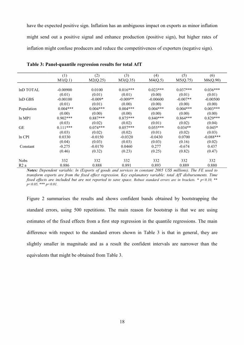
Table 3: Panel-quantile regression results for total AfT
(1) (2) (3) (4) (5) (6) M1(Q.1) M2(Q.25) M3(Q.35) M4(Q.5) M5(Q.75) M6(Q.90)
lnD TOTAL -0.00900 0.0100 0.016*** 0.023*** 0.037*** 0.036*** (0.01) (0.01) (0.01) (0.00) (0.01) (0.01) lnD GBS -0.00100 -0.009* -0.009** -0.00600 -0.007** -0.00500 (0.01) (0.01) (0.00) (0.00) (0.00) (0.00) Population 0.004*** 0.004*** 0.004*** 0.004*** 0.004*** 0.003*** (0.00) (0.00) (0.00) (0.00) (0.00) (0.00) ln MP1 0.902*** 0.887*** 0.875*** 0.840*** 0.864*** 0.829*** (0.03) (0.02) (0.02) (0.01) (0.02) (0.04) GE 0.111*** 0.074*** 0.057*** 0.055*** 0.034** 0.045* (0.03) (0.02) (0.02) (0.01) (0.02) (0.03) ln CPI 0.0330 -0.0150 -0.0320 -0.0430 0.0700 -0.088*** (0.04) (0.03) (0.03) (0.03) (0.16) (0.02) Constant -0.275 -0.0170 0.0460 0.277 -0.674 0.437 (0.46) (0.32) (0.23) (0.25) (0.82) (0.47) Nobs 332 332 332 332 332 332 R2 a 0.886 0.888 0.891 0.893 0.889 0.880
Notes: Dependent variable: ln (Exports of goods and services in constant 2005 US$ millions). The FE used to
transform exports are from the fixed effect regression. Key explanatory variable: total AfT disbursements. Time
fixed effects are included but are not reported to save space. Robust standard errors are in brackets. * p<0.10, **
p<0.05, *** p<0.01.
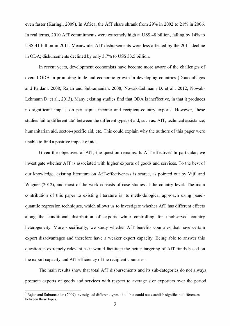
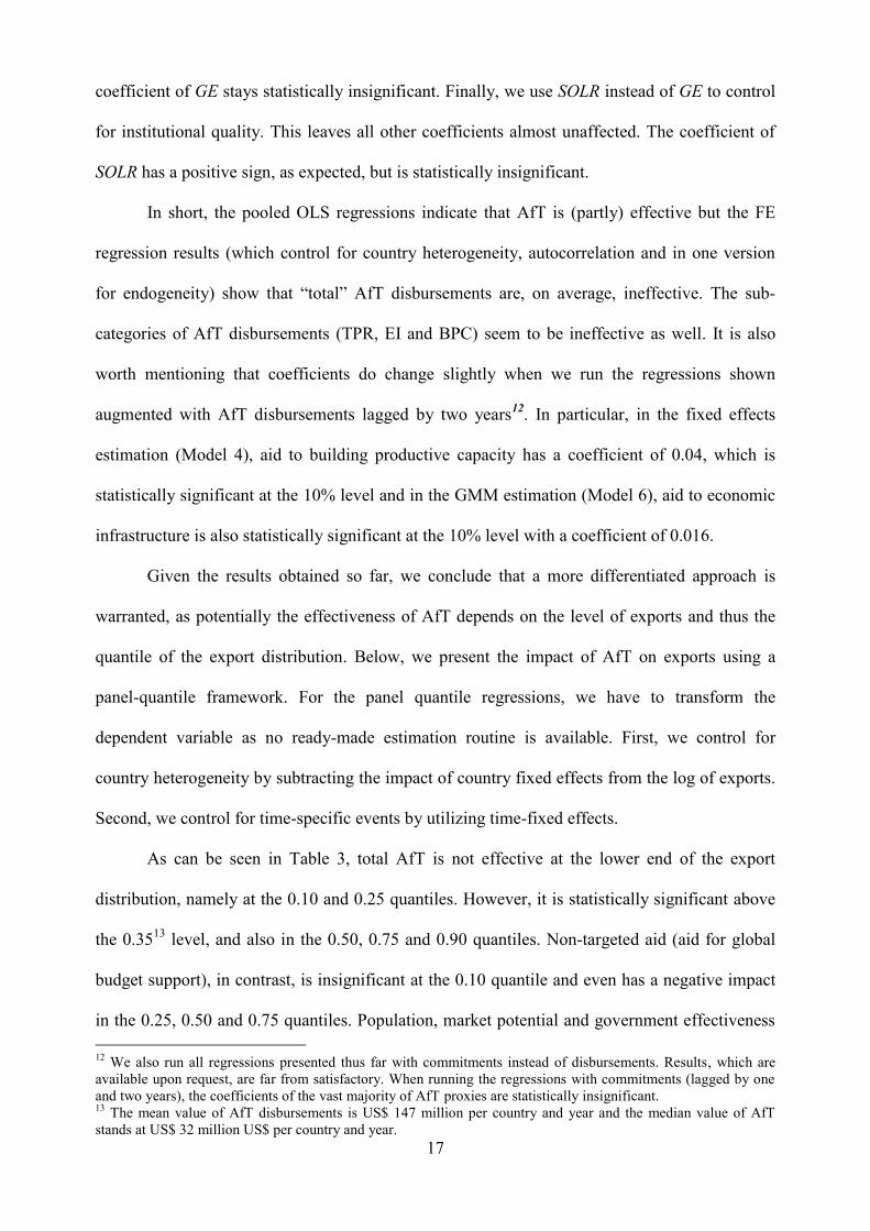
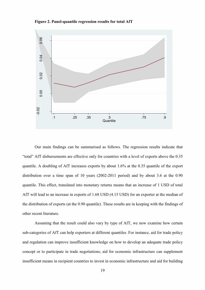
Figure 2 summarises the results and shows confident bands obtained by bootstrapping the
standard errors, using 500 repetitions. The main reason for bootstrap is that we are using
estimates of the fixed effects from a first step regression in the quantile regressions. The main
difference with respect to the standard errors shown in Table 3 is that in general, they are
slightly smaller in magnitude and as a result the confident intervals are narrower than the
equivalents that might be obtained from Table 3.
19
Figure 2. Panel-quantile regression results for total AfT
Our main findings can be summarised as follows. The regression results indicate that
“total” AfT disbursements are effective only for countries with a level of exports above the 0.35
quantile. A doubling of AfT increases exports by about 1.6% at the 0.35 quantile of the export
distribution over a time span of 10 years (2002-2011 period) and by about 3.6 at the 0.90
quantile. This effect, translated into monetary returns means that an increase of 1 USD of total
AfT will lead to an increase in exports of 1.68 USD (4.15 USD) for an exporter at the median of
the distribution of exports (at the 0.90 quantile). These results are in keeping with the findings of
other recent literature.
Assuming that the result could also vary by type of AfT, we now examine how certain
sub-categories of AfT can help exporters at different quantiles. For instance, aid for trade policy
and regulation can improve insufficient knowledge on how to develop an adequate trade policy
concept or to participate in trade negotiations; aid for economic infrastructure can supplement
insufficient means in recipient countries to invest in economic infrastructure and aid for building
-0.0
20
.00
0.0
20
.04
0.0
6
.1 .25 .35 .5 .75 .9Quantile
20
productive capacity can counteract insufficient means and knowledge related to under-
developed productive capacity in agriculture, industry and mining.
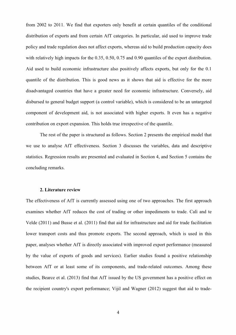
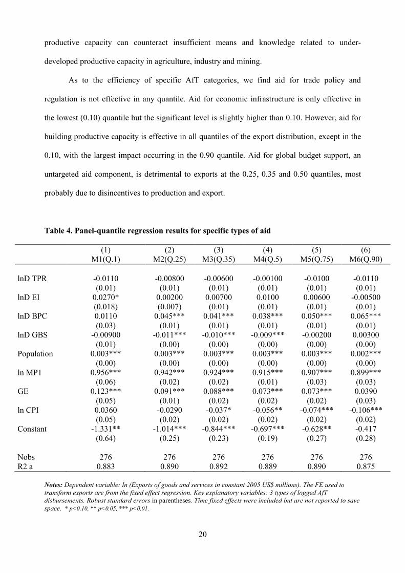
As to the efficiency of specific AfT categories, we find aid for trade policy and
regulation is not effective in any quantile. Aid for economic infrastructure is only effective in
the lowest (0.10) quantile but the significant level is slightly higher than 0.10. However, aid for
building productive capacity is effective in all quantiles of the export distribution, except in the
0.10, with the largest impact occurring in the 0.90 quantile. Aid for global budget support, an
untargeted aid component, is detrimental to exports at the 0.25, 0.35 and 0.50 quantiles, most
probably due to disincentives to production and export.
Table 4. Panel-quantile regression results for specific types of aid
(1) (2) (3) (4) (5) (6) M1(Q.1) M2(Q.25) M3(Q.35) M4(Q.5) M5(Q.75) M6(Q.90)
lnD TPR -0.0110 -0.00800 -0.00600 -0.00100 -0.0100 -0.0110 (0.01) (0.01) (0.01) (0.01) (0.01) (0.01) lnD EI 0.0270* 0.00200 0.00700 0.0100 0.00600 -0.00500 (0.018) (0.007) (0.01) (0.01) (0.01) (0.01) lnD BPC 0.0110 0.045*** 0.041*** 0.038*** 0.050*** 0.065*** (0.03) (0.01) (0.01) (0.01) (0.01) (0.01) lnD GBS -0.00900 -0.011*** -0.010*** -0.009*** -0.00200 0.00300 (0.01) (0.00) (0.00) (0.00) (0.00) (0.00) Population 0.003*** 0.003*** 0.003*** 0.003*** 0.003*** 0.002*** (0.00) (0.00) (0.00) (0.00) (0.00) (0.00) ln MP1 0.956*** 0.942*** 0.924*** 0.915*** 0.907*** 0.899*** (0.06) (0.02) (0.02) (0.01) (0.03) (0.03) GE 0.123*** 0.091*** 0.088*** 0.073*** 0.073*** 0.0390 (0.05) (0.01) (0.02) (0.02) (0.02) (0.03) ln CPI 0.0360 -0.0290 -0.037* -0.056** -0.074*** -0.106*** (0.05) (0.02) (0.02) (0.02) (0.02) (0.02) Constant -1.331** -1.014*** -0.844*** -0.697*** -0.628** -0.417 (0.64) (0.25) (0.23) (0.19) (0.27) (0.28) Nobs 276 276 276 276 276 276 R2 a 0.883 0.890 0.892 0.889 0.890 0.875
Notes: Dependent variable: ln (Exports of goods and services in constant 2005 US$ millions). The FE used to
transform exports are from the fixed effect regression. Key explanatory variables: 3 types of logged AfT
disbursements. Robust standard errors in parentheses. Time fixed effects were included but are not reported to save
space. * p<0.10, ** p<0.05, *** p<0.01.
21
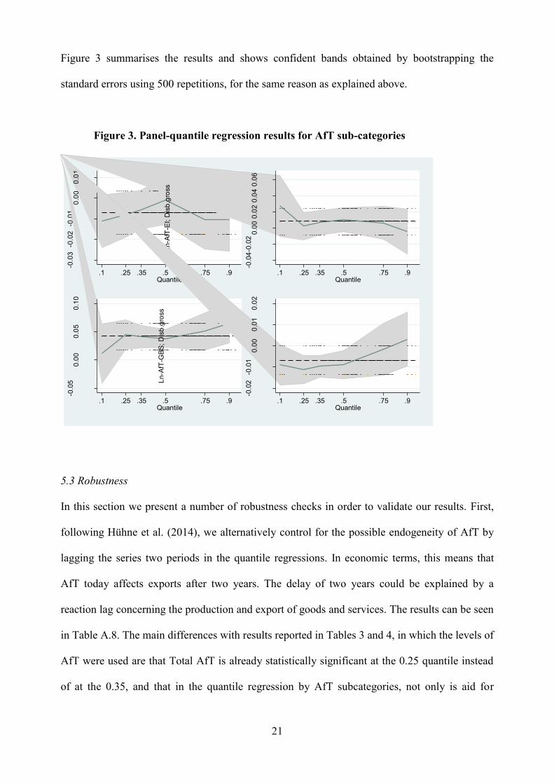
Figure 3 summarises the results and shows confident bands obtained by bootstrapping the
standard errors using 500 repetitions, for the same reason as explained above.
Figure 3. Panel-quantile regression results for AfT sub-categories
5.3 Robustness
In this section we present a number of robustness checks in order to validate our results. First,
following Hühne et al. (2014), we alternatively control for the possible endogeneity of AfT by
lagging the series two periods in the quantile regressions. In economic terms, this means that
AfT today affects exports after two years. The delay of two years could be explained by a
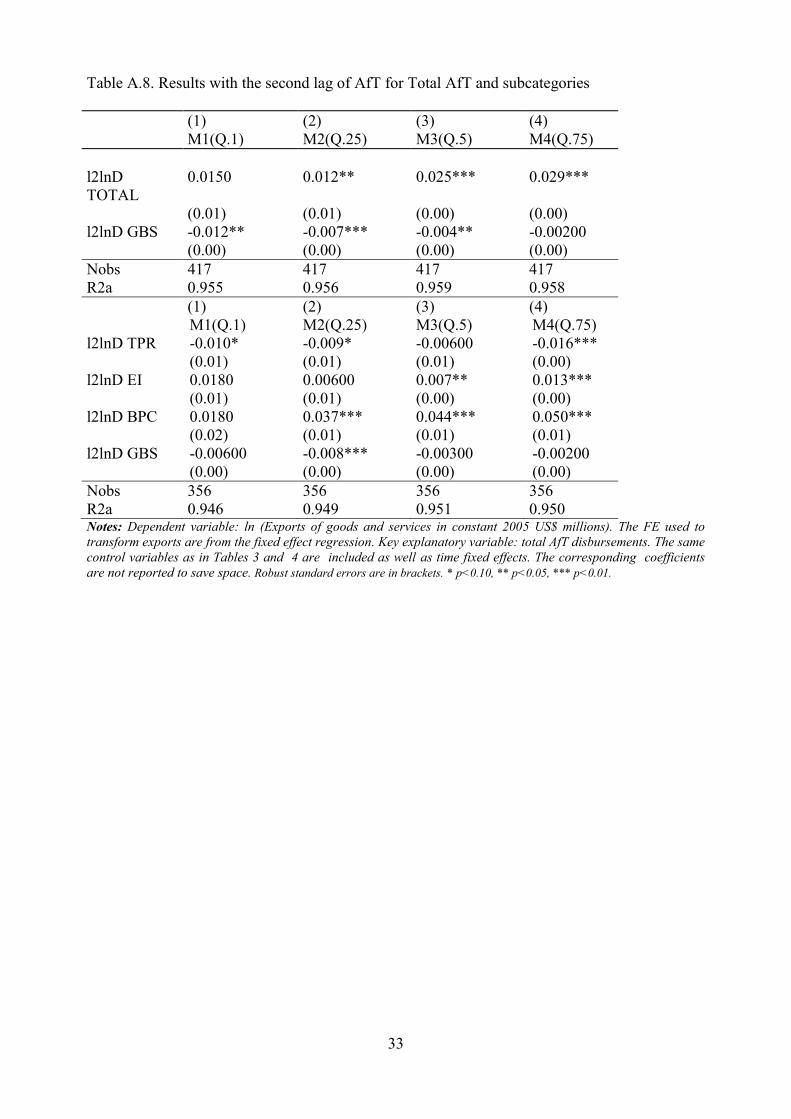
reaction lag concerning the production and export of goods and services. The results can be seen
in Table A.8. The main differences with results reported in Tables 3 and 4, in which the levels of
AfT were used are that Total AfT is already statistically significant at the 0.25 quantile instead
of at the 0.35, and that in the quantile regression by AfT subcategories, not only is aid for
-0.0
3-0
.02
-0.0
10
.00
0.0
1
.1 .25 .35 .5 .75 .9Quantile
-0.0
4-0
.02
0.0
00
.02
0.0
40
.06
Ln-A
fT-E
I; D
isb
.gro
ss
.1 .25 .35 .5 .75 .9Quantile
-0.0
50
.00
0.0
50
.10
.1 .25 .35 .5 .75 .9Quantile
-0.0
2-0
.01
0.0
00
.01
0.0
2
Ln-A
fT-G
BS
; D
isb
.gro
ss
.1 .25 .35 .5 .75 .9Quantile
22
building productive capacity positive and statistically significant, but so is aid for economic
infrastructure at the median value of exports and also at the 0.75 quantile.
Calì and te Velde (2011) tackled the endogeneity problem by employing instrumental variable
estimators. The instruments used for AfT are ‘respect for civil liberties and human rights’ and
the ‘affinity of nations’ (political proximity to the US, Japan, UK or France). Those authors
found that controlling for endogeneity changes the size of the coefficients, but the main
conclusion regarding AfT effectiveness remains the same.
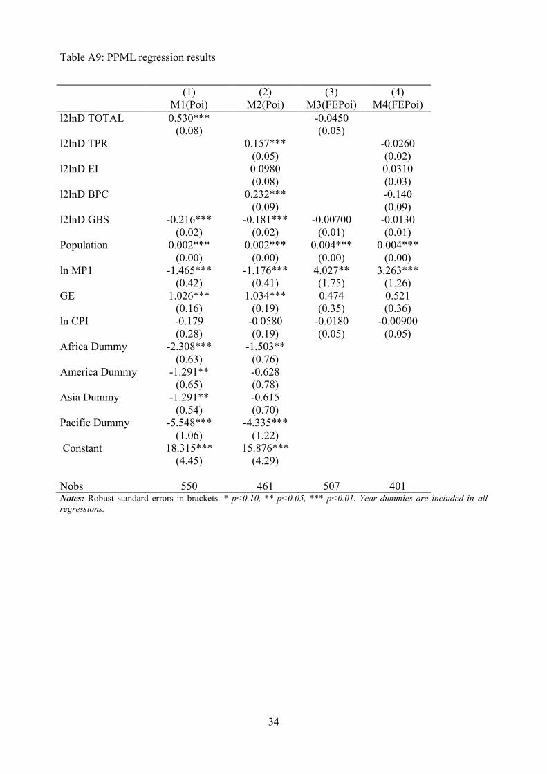
Second, to tackle the problem of “zero”-exports, we applied a Heckman two-step
procedure. We tried to identify a reasonable selection variable, however, with country-fixed
effects no other sensible variable qualified as a selection variable. In a common intercept model,
the status of legal rights (SOLR) could qualify as a selection variable but only with a confidence
level of 82%. As an alternative, we applied Pseudo Maximum Likelihood estimation (PPML).
The results for the different AfT components for the model without and with country fixed
effects are similar to the ones found in Table 2 (see Table A.9).
Third, controlling for missing values in the AfT variables was not possible either as
generating an AfT-dummy variable (i.e. replacing the “na” values by zeros and setting the
positive AfT-values to “1”) led to perfect multicollinearity between the AfT-variables and the
AfT-dummy. However, according to Calì and te Velde (2011), missing values for the Aft
variables are not an imminent problem. Most missing values cannot be observed for exports.
Finally, we also estimated similar models without the control aid for general budget
support. The main results obtained for target AfT variables remained the same.
Summarising, the estimation of the impact of AfT on different quantiles of the export
distribution seems warranted as only this procedure takes into account the heterogeneity of
impacts along the distribution of exports and produces stable results.
6. Conclusions

23
It is widely acknowledged that one of the main objectives of AfT is to promote exports of goods
and services. Given said aim, this paper examines the extent to which AfT is effective in
promoting trade, particularly in countries with a weak export capacity. To this end, we analyse
whether AfT and its different components are associated with higher exports of goods and
services, quantify the effects and examine whether these effects depend on the conditional
distribution of exports and the time frame studied.
We find that AfT-disbursements (also of different types) are not effective in conditional
mean panel regression models (standard regression models) with country fixed effects. Using
panel quantile regressions we find that total AfT disbursements are effective at the 0.35 quantile
of the distribution of exports, where they promote exports of goods and services. However, AfT
is not effective at the lower tails (0.1 and 0.25 quantiles). All things being equal, a 100%
increase of “total” AfT disbursements is associated with an increase in exports of around 2-3%
depending on the quantile and taken over a 10-year time period. On an annual basis, this would
leave the recipient countries with a 0.2% increase in exports as a result of AfT.
We also find that specific types of AfT are effective to differing extents. We find evidence that
AfT to support trade policy and regulation is not effective in any quantile of the export
distribution, but this type of AfT represents less than 5% of total AfT. Aid disbursed to building
production capacity (BPC) is effective in almost all quantiles of the export distribution.
Doubling BPC leads to an increase in exports of around 4.5-6.5%. However, it is worth
mentioning that this sub-type of AfT reaches maximum impact in the 0.90 quantile. This could
mean that smaller exporters with a more reduced basis in knowledge and experience profit less
from AfT for BPC. For instance, this type of aid is sector-specific and can take the form of
technical assistance (training provided by experts) and/or transfers in the form of grants and
loans. Effectiveness of aid for EI is effective at the 0.10 quantile when using. Doubling
infrastructure-related aid in this quantile leads to a 0.27% increase of exports. Therefore, an
increase of AfT for economic infrastructure would be especially helpful to less mature
24
exporters. In comparison, aid disbursed under GBS is generally not associated with higher
exports. It seems to be rather counter-productive, even showing a negative effect on exports, and
hence apparently not improving the business environment.
In conclusion and in comparison with other studies, we find that aid disbursed to TPR is
a category of AfT that seems not to be effective irrespective of the exported amount. This result
is not in line with the findings of Hühne et al. (2014) whose findings indicate that AfT to TPR
has the strongest impact. According to our results, aid for building productive capacity (BPC) is
effective in almost all quantiles of the export distribution and also has the largest impact on
exports. Furthermore, our results indicate that certain types of AfT, such as AfT for economic
infrastructure, which is considered as generally effective by Calì and te Velde (2011), is only
effective at the lowest quantile of the distribution of exports.
Further research should examine the topic of AfT effectiveness in greater detail. To date,
we know that some types of AfT are effective in promoting exports, whereas others are not so
effective. An important focus of further research should be to examine why some types of AfT
are less effective. Additionally, the relationship between AfT and a number of social outcomes
(such as poverty rates) also warrant further examination, as increased trade is only a means to an
end and not an end in itself.
25
References
Adhikari R (2011). Evaluating Aid for Trade Effectiveness on the Ground: A Methodological
Framework. Aid for Trade Series, Issue Paper No. 20, International Centre for Trade and
Sustainable Development, Geneva, Switzerland.
Bearce D Finkel S E, Pérez Liñán A, Rodriquez-Zepeda J, Surzhko-Harned L (2013). Has Aid
for Trade Increased Recipient Exports? The Impact of US AfT Allocations 1999-2008.
International Studies Quarterly, Vol. 57 (1), pp.163-170.
Busse, M., Hoekstra, R. and Königer, J. (2011). The impact of aid for trade facilitation on the
costs of trading. Paper presented at CSAE 2011.
Calì M and Te Velde D (2011). Does Aid for Trade Really Improve Trade Performance? World
Development, Vol. 39(5), pp. 725-740.
Canay, I. (2011). A Simple Approach to Quantile Regression for Panel Data” The Econometrics
Journal 14, 368-386.
CEPII (2013a). CEPII`s Databases. Distances (geo_cepii, dist_cepii).
http://www.cepii.fr/anglaisgraph/bdd/bdd.htm. Accessed: 20/09/13.
Doucouliagos, H and Paldam, M (2008). Aid effectiveness on growth: A meta study. The
European Journal of Political Economy, 248(1), 1-24.
Foreign Policy (2011). The Failed States Index 2011.
Available online: http://www.foreignpolicy.com/failedstates. Accessed: 20/09/13.
García, M (2008) Monitoring Aid for Trade, London, CUTS, 5th June 2008, http://www.cuts-
london.org/events/documents/CUTS05jun.pdf.
Hanke S (2008). Zimbabwe: From Hyperinflation to Growth. The Cato Institute. Development
Policy Analysis, 2008, No. 6.
Available online: http://www.cato.org/pub_display.php?pub_id=9484.Accessed:
20/09/13.
Harris C (1954). The Market as a Factor in the Localization of Industry in the United States.
Annals of the Association of American Geographers, Vol. 44(4), pp.315-348.
Helble M, Mann C and Wilson J (2012). Aid for Trade Facilitation. Review of World Economics
148 (2), 357-376.
Hoechle D (2007). Robust Standard Errors for Panel Regressions with Cross-sectional
Dependence. The Stata Journal, Vol. 7(3), pp. 281-312.
Huchet-Bourdon, M, Lipchitz, A and Rousson, A (2009) Aid for Trade in Developing
Countries: Complex Linkages for Real Effectiveness. African Development Review,
21(2), 243-290.
26
Hühne, P, Meyer, B and Nunnenkamp, P (2014) Who Benefits from Aid for Trade? Comparing
the Effects on Recipient versus Donor Exports. Journal of Development Studies 50 (9)
.1275-1288.
Karingi, S (2009) Towards the Global Review of Aid for Trade 2009. Issues and State of
Implementation in Africa. UN Economic Commission for Africa.
http://www1.uneca.org. Accessed 28/01/14.
Luke, D (2009) Africa and Aid for Trade: What are the Trends? What are the Issues?
AFRICAVIEWPOINT No. 11, August 2009. Regional Bureau for Africa. United
Nations Development Programme (UNDP).
http://www.undg.org/Africa/africaviewpoint/2009-august.pdf.
Lutz W and KC S (2010). Dimensions of Global Population Projections: What Do We Know
About Future Population Trends and Structures? Philosophical Transactions of the Royal
Society B, Vol. 365, pp. 2779-2791.
Nowak-Lehmann D., F, Dreher, A, Herzer, D, Klasen, S and Martínez-Zarzoso, I (2012). Does
foreign aid really raise per capita income? A time series perspective. Canadian Journal
of Economics, 45(1), 288-313.
Nowak-Lehmann, F, Martínez-Zarzoso, I, Herzer, D, Klasen, S and Cardozo, A (2013). Does
foreign aid promote exports to donor countries? Review of World Economics, 149(3),
505-535.
OECD/WTO (2011). Aid for Trade and LDCs: Starting to Show Results.
Available online: http://www.oecd.org/dataoecd/18/53/47706423.pdf. Accessed:
20/09/13.
OECD (2013a). Creditor Reporting System (CRS) Database.
http://stats.oecd.org/Index.aspx?DataSetCode=CRSNEW. Accessed: 20/09/13.
OECD (2013b). Creditor Reporting System (CRS) Database. Metadata. Database Specific.
Abstract.
http://stats.oecd.org/Index.aspx?DataSetCode=CRSNEW. Accessed: 20/09/13.
OECD (2013c). Aid-for-Trade Proxies.
Available online: http://www.oecd.org/dataoecd/29/1/39880833.pdf. Accessed:
20/09/13.
OECD (2014) Aid for Trade. http://www.oecd.org/dac/aft/aid-for-tradestatisticalqueries.html
Accessed 28/01/14.
27
Overman H, Redding S and Venables A (2001). The Economic Geography of Trade Production
and Income: A Survey of Empirics. Centre for Economic Policy Research (CEPR).
Discussion Paper (2978).
Rajan, R and Subramanian, A (2008) Aid and growth: What does the cross-country evidence
really show? Review of Economics and Statistics, 90(4), 643-665.
Vijil M and Wagner L (2012). Does Aid for Trade Enhance Export Performance? Investigating
on the Infrastructure Channel. World Economy 35 (7), 838-868.
Wooldridge J (2001). Econometric Analysis of Cross Section and Panel Data. Cambridge, MA:
MIT Press.
Wooldridge J (2003). Introductory Econometrics: A Modern Approach, 2nd ed. Cincinnati, OH:
South-Western College Publishing.
World Bank (2013a). World Development Indicators (WDI).
http://databank.worldbank.org/ddp/home.do. Accessed: 20/09/13.
World Bank (2013b). Worldwide Governance Indicators (WGI).
http://info.worldbank.org/governance/wgi/index.asp. Accessed: 20/09/13.
28
Sector-
numberSector
AfT-proxy/Aid-
proxyAbbr.
331 Trade Policy and Regulations
Trade Policy and
Regulations
(TPR)
A4T_TPR
210 Transport and Storage
220 Communications
230 Energy Generation and Supply
240 Banking and Financial Services
250 Business and Other Services
311 Agriculture
312 Forestry
313 Fishing
321 Industry
322 Mineral Resources and Mining
332 Tourism
Building Productive
Capacity (BPC)
Economic
Infrastructure
(EI)
A4T_EI
A4T_BPC
A4T_TO
TA
L
Table A.1. Composition of AfT categories
Notes: Illustrations are based partly on OECD (2013c). AfT proxies are calculated as the sum of ODA for the three
corresponding sectors as shown in the table. For example, EI is calculated as the sum of ODA for the five sub-
sectors, “Transport and Storage”, “Communications”, “Energy Generation and Supply”, “Banking and Financial Services” and “Business and other Services”. If data on ODA for some sectors was missing, the AfT proxy was
calculated as the sum of ODA for the other sectors, i.e. when calculating the sum over all corresponding sectors,
missing values are set equal to 0 as long as all values are missing (in which case the AfT proxy would be missing
too). Abbr.: Abbreviations.
29
Table A.2. ADF Fisher unit root tests
ADF-Fisher Chi-square statistic
p-value
Ln exports 201.94 0.68
LnAfT 185.73 1.00
LnAfT_TPR 177.15 0.23
LnAfT_EI 211.83 0.99
LnAfT_BPC 272.19 0.45
LnAid_GBS 41.89 0.96
Pop 186.87 1.00
LnMp1 89.15 1.00
GE 272.67 0.81
LnCpi 176.80 1.00
Note: Null hypothesis: Unit root, ie. the series is non-stationary. Probabilities for Fisher ADF tests are calculated using an asymptotic Chi-square distribution.
Table A.3. Kao’s residual cointegration test and Pesaran’s (2011) cointegration test
Kao ADF t-statistic p-value
Cointegration between lnExports, LnAfT, LnAid_GBS, Pop, LnMp1, GE, LnCpi
1.32* 0.09
Cointegration between lnExports, LnAfT_TPR, LnAfT_EI, LnAfT_BPC, LnAid_GBS, Pop, LnMp1, GE, LnCpi
2.93*** 0.01
Pesaran’s et al. (2011) ARDL bounds testing
F-statistic Pesaran’s critical values
I(0) I(1)
Cointegration between lnExports, LnAfT, LnAid_GBS, Pop, LnMp1, GE, LnCpi
14.46*** F(7, 251) 2.96 4.26
Cointegration between lnExports, LnAfT_TPR, LnAfT_EI, LnAfT_BPC, LnAid_GBS, Pop, LnMp1, GE, LnCpi
1.67 E+11*** F(9, 196) 2.65 3.97
Note: Null hypothesis: No cointegration, respectively the right-hand side variables are not significantly different
from zero.

30
Table A.4. List of countries
Afghanistan Equatorial Guinea Pakistan
Angola Grenada Panama
Albania Guatemala Peru
Argentina Guyana Philippine
Armenia Honduras Palau
Antigua and Barbuda Croatia Papua New Guinea
Azerbaijan Haiti Paraguay
Burundi Indonesia Rwanda
Benin India Saudi Arabia
Burkina Faso Iran, Islamic Rep. Sudan
Bangladesh Iraq (no exports) Senegal
Bahrain Jamaica Solomon Islands
Bosnia and Herzegovina Jordan Sierra Leone
Belarus Kazakhstan El Salvador
Belize Kenya Sao Tome and Principe
Bolivia Kyrgyz Republic Suriname
Brazil Cambodia Slovenia
Barbados St. Kitts and Nevis Swaziland
Bhutan Lao PDR Seychelles
Botswana Lebanon Syrian Arab Republic
Central African Republic Liberia Chad
Chile Libya Togo
China St. Lucia Thailand
Cote d'Ivoire Sri Lanka Tajikistan
Cameroon Lesotho Turkmenistan
Congo, Rep. Morocco Tonga
Colombia Moldova Trinidad and Tobago
Comoros Madagascar Tunisia
Cape Verde Maldives Turkey
Costa Rica Mexico Tanzania
Cuba Macedonia, FYR Uganda
Djibouti Mali Ukraine
Dominica Malta Uruguay
Dominican Republic Mongolia Uzbekistan
Algeria Mozambique St. Vincent and the Grenadines
Ecuador Mauritania Venezuela, RB
Egypt, Arab Rep. Mauritius Vietnam
Eritrea Malawi Vanuatu
Ethiopia Malaysia Samoa
Fiji Namibia Yemen, Rep.
Gabon Niger South Africa
Georgia Nigeria Congo, Dem. Rep.
Ghana Nicaragua Zambia
Guinea Nepal Zimbabwe
Gambia, The Oman
31
Table A.5. List of variables, abbreviations, description and sources
Variable Variable description Source
AfT
-varia
ble
s (
targ
ete
d)
an
d a
id c
on
tro
l varia
ble
C_TPR A4T proxy for Trade Policy and Regulations; Commitments* own calculations; CRS
C_EI A4T proxy for Economic Infrastructure; Commitments* own calculations; CRS
C_BPC A4T proxy for Building Productive Capacity; Commitments* own calculations; CRS
C_TOTAL A4T proxy Total; Commitments* own calculations; CRS
C_GBS Untargeted AID, proxy for General Budget Support; Commitments*
own calculations; CRS
D_TPR A4T proxy for Trade Policy and Regulations; Disb. gross* own calculations; CRS
D_EI A4T proxy for Economic Infrastructure; Disb. gross* own calculations; CRS
D_BPC A4T proxy for Building Production Capacity; Disb. gross* own calculations; CRS
D_TOTAL A4T proxy Total; Disbursements gross* own calculations; CRS
D_GBS Untargeted AID, proxy for General Budget Support; Disb. gross* own calculations; CRS
Dep
en
den
t
varia
ble
an
d
imp
ort
an
t co
ntr
ols
Exports Exports of goods and services (constant 2005 USD millions) WDI
Population Population, total (in millions) WDI
MP1 Market Potential 1 (with simple distances) own calc.; WDI, CEPII
GE Government Effectiveness (-2.5=weak to 2.5=strong gov. performance)
WGI
CPI Consumer price index (2005 = 100) WDI
Oth
er
co
ntr
ols
MP2 Market Potential 2 (with square root distances) own calc.; WDI, CEPII
MP3 Market Potential 3 (with squared distances) own calc.; WDI, CEPII
SOLR Strength of legal rights index (0=weak to 10=strong) WDI
Notes: * constant 2011 US$ millions. CEPII: Centre d'Etudes Prospectives et d'Informations Internationales, CEPII (2011a/b);
CRS: Creditor Reporting System, OECD (2013a); Disb.: Disbursements; Gov.: government or governance; own calc.: own
calculations; WDI: World Development Indicators, World Bank (2011a); WGI: World Governance Indicators, World Bank
(2011b).
Table A.6. AfT commitments and disbursements
Target
Variables
Obs Mean Std. Dev. Min Max
Commitments
C_TPR 1312 4.631 17.779 0.000 461.053
C_EI 1662 142.824 317.260 0.000 4264.45
C_BPC 1684 58.618 119.746 0.000 1926.927
C_TOTAL 1699 201.391 409.525 0.000 5375.200
C_GBS 810 87.058 159.957 0.00 1730.520
Disbursements
D_TPR 1204 3.360 15.781 0.000 403.724
D_EI 1404 103.006 217.144 0.006 2386.488
D_BPC 1415 44.714 80.960 0.003 775.843
D_TOTAL 1425 148.7273 288.606 0.003 3042.281
D_GBS 742 70.240 122.008 0.00 1066.810
32
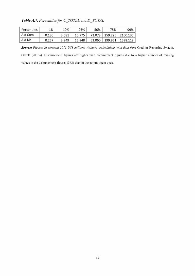
Table A.7. Percentiles for C_TOTAL and D_TOTAL
Percentiles 1% 10% 25% 50% 75% 99%
Aid Com 0.130 3.681 15.775 73.078 259.225 2160.135
Aid Dis 0.257 3.949 15.848 63.060 199.951 1598.119
Source: Figures in constant 2011 US$ millions. Authors’ calculations with data from Creditor Reporting System,
OECD (2013a). Disbursement figures are higher than commitment figures due to a higher number of missing
values in the disbursement figures (363) than in the commitment ones.
33
Table A.8. Results with the second lag of AfT for Total AfT and subcategories
(1) (2) (3) (4) M1(Q.1) M2(Q.25) M3(Q.5) M4(Q.75)
l2lnD TOTAL
0.0150 0.012** 0.025*** 0.029***
(0.01) (0.01) (0.00) (0.00) l2lnD GBS -0.012** -0.007*** -0.004** -0.00200 (0.00) (0.00) (0.00) (0.00)
Nobs 417 417 417 417 R2a 0.955 0.956 0.959 0.958
(1) (2) (3) (4) M1(Q.1) M2(Q.25) M3(Q.5) M4(Q.75) l2lnD TPR -0.010* -0.009* -0.00600 -0.016*** (0.01) (0.01) (0.01) (0.00) l2lnD EI 0.0180 0.00600 0.007** 0.013*** (0.01) (0.01) (0.00) (0.00) l2lnD BPC 0.0180 0.037*** 0.044*** 0.050*** (0.02) (0.01) (0.01) (0.01) l2lnD GBS -0.00600 -0.008*** -0.00300 -0.00200 (0.00) (0.00) (0.00) (0.00)
Nobs 356 356 356 356 R2a 0.946 0.949 0.951 0.950 Notes: Dependent variable: ln (Exports of goods and services in constant 2005 US$ millions). The FE used to
transform exports are from the fixed effect regression. Key explanatory variable: total AfT disbursements. The same
control variables as in Tables 3 and 4 are included as well as time fixed effects. The corresponding coefficients
are not reported to save space. Robust standard errors are in brackets. * p<0.10, ** p<0.05, *** p<0.01.
34
Table A9: PPML regression results
(1) (2) (3) (4) M1(Poi) M2(Poi) M3(FEPoi) M4(FEPoi)
l2lnD TOTAL 0.530*** -0.0450 (0.08) (0.05) l2lnD TPR 0.157*** -0.0260 (0.05) (0.02) l2lnD EI 0.0980 0.0310 (0.08) (0.03) l2lnD BPC 0.232*** -0.140 (0.09) (0.09) l2lnD GBS -0.216*** -0.181*** -0.00700 -0.0130 (0.02) (0.02) (0.01) (0.01) Population 0.002*** 0.002*** 0.004*** 0.004*** (0.00) (0.00) (0.00) (0.00) ln MP1 -1.465*** -1.176*** 4.027** 3.263*** (0.42) (0.41) (1.75) (1.26) GE 1.026*** 1.034*** 0.474 0.521 (0.16) (0.19) (0.35) (0.36) ln CPI -0.179 -0.0580 -0.0180 -0.00900 (0.28) (0.19) (0.05) (0.05) Africa Dummy -2.308*** -1.503** (0.63) (0.76) America Dummy -1.291** -0.628 (0.65) (0.78) Asia Dummy -1.291** -0.615 (0.54) (0.70) Pacific Dummy -5.548*** -4.335*** (1.06) (1.22) Constant 18.315*** 15.876*** (4.45) (4.29) Nobs 550 461 507 401 Notes: Robust standard errors in brackets. * p<0.10, ** p<0.05, *** p<0.01. Year dummies are included in all
regressions.
35
Figure A.1. Regional distribution of countries included in our analysis
Notes: Figures based on author’s calculations. Data are from CEPII (2011a). Shares add up to 1.