Quantile Graphical Models: Bayesian Approaches

Nilabja Guha+, Veera Baladandayuthapani ++,Bani K. Mallick∗

+ Department of Mathematical Sciences, University of MassachusettsLowell, Lowell, MA 01854, USA.

∗ Department of Statistics, Texas A & M University, College Station, TX77843, USA.

++ Department of Biostatistics, University of Michigan, Ann Arbor, MI48103, USA.

February 20, 2020

Abstract

Graphical models are ubiquitous tools to describe the interdependence betweenvariables measured simultaneously such as large-scale gene or protein expression data.Gaussian graphical models (GGMs) are well-established tools for probabilistic explo-ration of dependence structures using precision matrices and they are generated undera multivariate normal joint distribution. However, they suffer from several shortcom-ings since they are based on Gaussian distribution assumptions. In this article, wepropose a Bayesian quantile based approach for sparse estimation of graphs. Wedemonstrate that the resulting graph estimation is robust to outliers and applicableunder general distributional assumptions. Furthermore, we develop efficient varia-tional Bayes approximations to scale the methods for large data sets. Our methodsare applied to a novel cancer proteomics data dataset where-in multiple proteomicantibodies are simultaneously assessed on tumor samples using reverse-phase proteinarrays (RPPA) technology.

Key-words : Graphical model, Quantile regression, Variational Bayes

1

1 Introduction

Probabilistic graphical models are the basic tools to represent dependence structures amongmultiple variables. They provide a simple way to visualize the structure of a probabilisticmodel as well as provide insights into the properties of the model, including conditionalindependence structures. A graph comprises with vertices (nodes) connected by edges(links or arcs). In a probabilistic graphical model, each vertex represents a random variable(single or vector) and the edges express probabilistic relationship between these variables.The graph defines the way the joint distribution over all the random variables can bedecomposed into a product of factors contacting subset of the variables. There are two typesof probabilistic graphical models: (1) Undirected graphical models where the edges do notcarry the directional information (Schafer and Strimmer, 2005; Dobra et al., 2004; Yuan andLin, 2007); (2) The other major class of graphical models is the directed graphical models(DAG) or Bayesian networks where the edges of the graphs have a particular directionalitywhich expresses causal relationships between random variables (Friedman, 2004; Segal etal., 2003; Mallick et al. 2009). In this paper, we focus on the undirected graphical models.

One popular tool of undirected graphical models is Gaussian Graphical Models (GGM)which assume that the stochastic variables follow a multivariate normal distribution witha particular structure of the inverse of the covariance matrix, called the precision or theconcentration matrix. This precision matrix of the multivariate normal distribution has theinterpretation of the conditional dependence. Compared with the marginal dependence,this conditional dependence can capture the direct link between two variables when all othervariables are conditioned on. Furthermore, it is usually assumed that one of the variablescan be predicted by those of a small subset of other variables. This assumption leadsto sparsity (many zeros) in the precision matrix and reduces the problem to well knowncovariance selection problems (Dempster, 1972; Wong et al.,2003). Sparse estimation ofprecision matrix, thus plays a center role in Gaussian graphical model estimation problem(Friedman et al., 2008).

There has been an intense development of Bayesian graphical model literature overthe past decades but mainly in a Gaussian graphical model setup. In a Bayesian setup,this joint modeling is done by hierarchically specifying priors on inverse covariance ma-trix (or precision matrix) using global priors on the space of positive-definite matrices.This prior specification is done through inverse Wishart priors or hyper-inverse Wishartpriors (Lauritzen,1996). Wishart priors show conjugate formulation and exact marginallikelihoods can be computed (Scott and Carvalho, 2008) but overall inflexible due to itsrestrictive forms. In the space of decomposable graph the marginal likelihood are available

2

upto normalizing constants (Giudici, 1996; Roverato, 2000). The marginal likelihoods areused to calculate the posterior probability of each graph, resulting an exact solution forsmaller dimension but for a moderately large P (number of nodes) or outside such restrictiveclass the computation may be prohibitively expensive. For non decomposable graph thecomputation is non trivial and maybe prohibitive using reversible jump MCMC (Giudiciand Green, 1999; Brooks et al, 2003). A novel Monte Carlo technique can be found inAtay-Kayis and Massam (2005). There have been approaches by shrinking the covariancematrix using matrix factorization. For example, factorization of covariance matrix in termsof standard deviation and correlation (Barnard et al., 2000), decomposition of correlationmatrix (Liechty et al., 2004) explore such technique. Writing the inverse covariance matrixas the product of inverse partial variance and the matrix of partial correlations, Wong etal. (2003) used reversible-jump-based Markov chain Monte Carlo (MCMC) algorithms toidentify the zeros among the off-diagonal elements.

An equivalent formulation of GGM is via neighborhood selection through the condi-tional mean under normality assumption (Peng et al. 2009). The method is based on theconditional distribution of each variable, conditioning on all other variables. In a GGMframework, this conditional distribution is a normal distribution with the conditional meanfunction linearly related to the other variables. Furthermore, the conditional independencerelationship among variables can be inferred by the variable selection techniques of the re-gression coefficients of the conditional mean function (Meinshausen and Buhlmann (2006)).More specifically, if a specific regression coefficient appeared to be zero, the correspondingvariables are conditionally independent. Of course, the joint distribution approach and theconditional approach based on linear regressions are essentially equivalent.

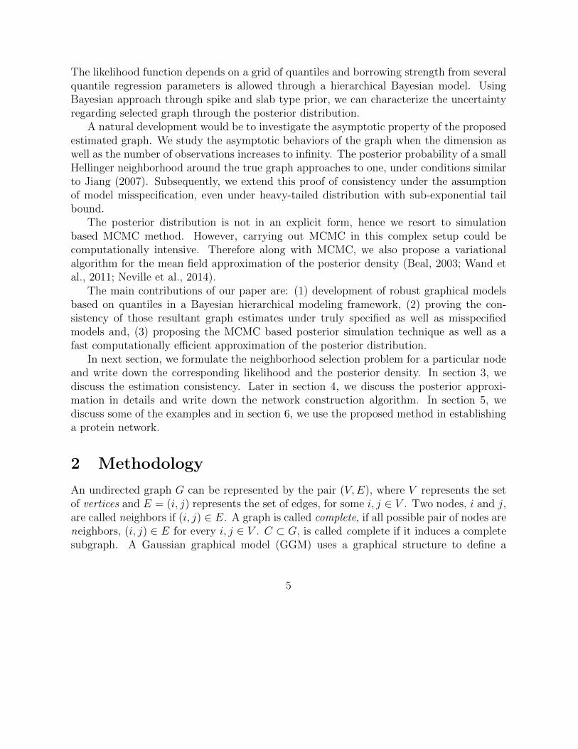
Due to ease of computation and the presence of a nice interpretation, the vast majorityof works on graphical model selection have been centered around the multivariate Gaussiandistribution. In a multivariate Gaussian setup the conditional mean conveys necessary andsufficient information to infer the conditional independence structure. In contrast, forother distributions, this may not be true. For instance, for the multivariate t-distribution,the conditional independence can not be captured only using the conditional mean as italso depends on the conditional variance which is a nonlinear function of other variables(Kotz and Nadarajah, 2004). For more complex distributions, the conditional independencestructure may depend nonlinearly on higher order moments of the conditional distribution.Hence, the inference of a graph can be significantly affected by deviations from the normalityand can lead to a wrong graph. The following example, which we discuss in details in section5 (Example 1 (a)), demonstrates the effect of deviation from normality in a simple case.We assume the following structure for a graph with 30 variables/nodes X1, . . . , X30 with

3

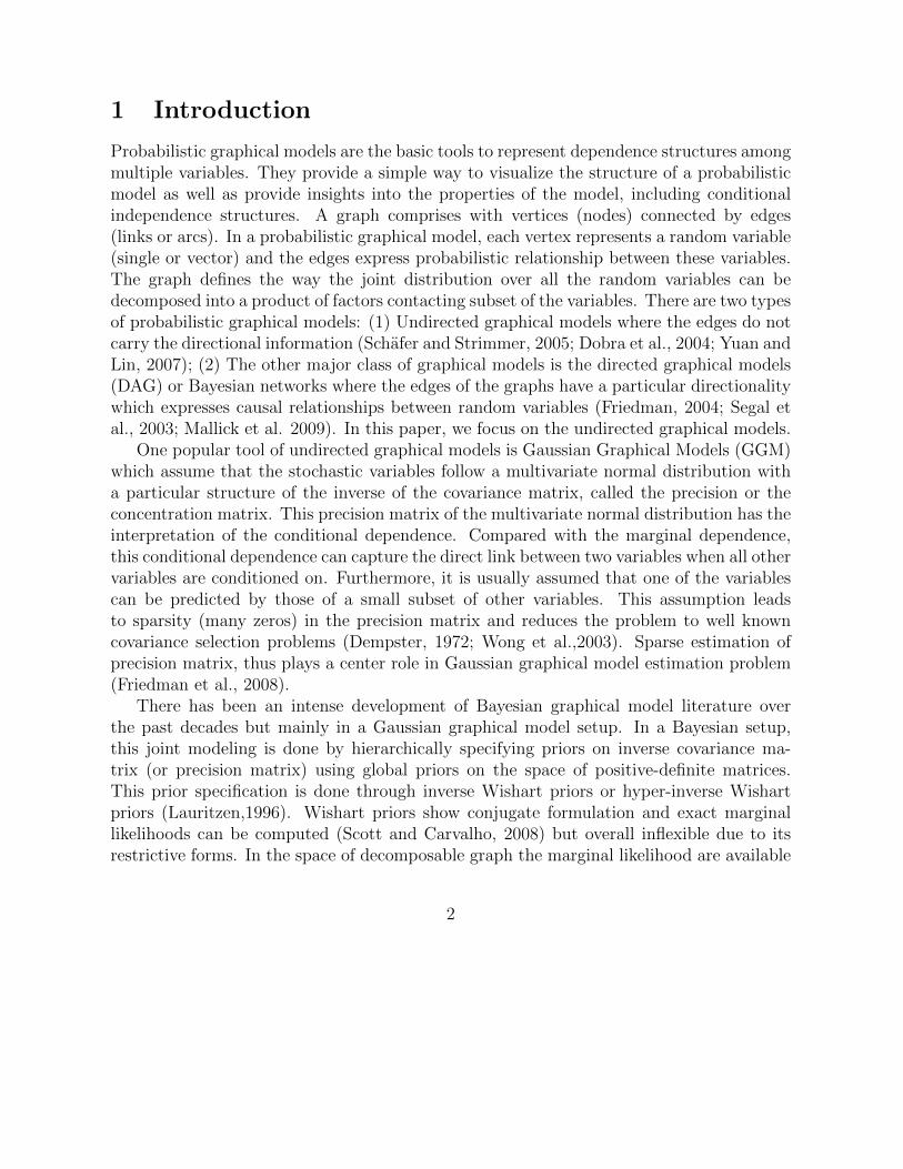
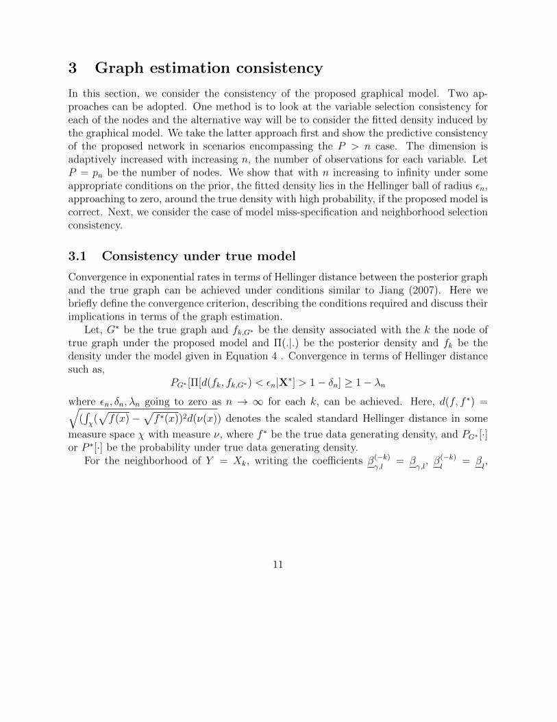
Figure 1: Left panel shows the true graph and right panel shows GGM fit in a typical case.

400 observations from each variable. Here X11, . . . , X20 is generated from a heavy taileddistribution induced by a common scale parameter, and Xi, Xj. i, j ≤ 10 is connected inthe network iff |i− j| < 2, given the scale parameter, and X1 . . . , X9 has some nonlinearityand non-normality and they form a subgraph G1 disjoint from G2 formed by X11, . . . , X20.We have X20, . . . , X29 independent of the rest and X30 is the function of the latent scaleparameter. The fitted and true graphs for X1, . . . , X29 given the scale parameter, are givenin Figure 1 where index i denotes i th vertex corresponding to Xi, and it is clear thatwith deviation from Gaussianity we have a large number of falsely detected edges. Thisposes serious restriction in a variety of applications which contain non-Gaussian data aswell as data with outliers. Liu et al. (2012) used Gaussian Copula model to allow flexiblemarginal distributions. Alternatively, non-Gaussian distributions have been directly usedfor modeling the joint distribution to obtain the graph (Finegold and Drton, 2011; Yanget al., 2014).

In this paper, we propose a novel Bayesian quantile based graphical model. The mainintention is to model the conditional quantile functions (rather than the mean) in a regres-sion setup. This is well known that the conditional quantile regression coefficients can inferthe conditional independence between variables. Under linearity of the conditional quantileregression function, conditional distribution of the kth variable is independent of the jthvariable if the corresponding regression coefficient of the quantile regression is zero for allquantiles. Hence by performing a neighborhood selection of these quantile regression coef-ficients, we can explore the graphical structure. Thus, in our framework this neighborhoodselection boils down to a variable selection problem in the quantile regression setup. A spikeand slab prior formulation has been used for that purpose (George and McCulloch, 1993).

4

The likelihood function depends on a grid of quantiles and borrowing strength from severalquantile regression parameters is allowed through a hierarchical Bayesian model. UsingBayesian approach through spike and slab type prior, we can characterize the uncertaintyregarding selected graph through the posterior distribution.

A natural development would be to investigate the asymptotic property of the proposedestimated graph. We study the asymptotic behaviors of the graph when the dimension aswell as the number of observations increases to infinity. The posterior probability of a smallHellinger neighborhood around the true graph approaches to one, under conditions similarto Jiang (2007). Subsequently, we extend this proof of consistency under the assumptionof model misspecification, even under heavy-tailed distribution with sub-exponential tailbound.

The posterior distribution is not in an explicit form, hence we resort to simulationbased MCMC method. However, carrying out MCMC in this complex setup could becomputationally intensive. Therefore along with MCMC, we also propose a variationalalgorithm for the mean field approximation of the posterior density (Beal, 2003; Wand etal., 2011; Neville et al., 2014).

The main contributions of our paper are: (1) development of robust graphical modelsbased on quantiles in a Bayesian hierarchical modeling framework, (2) proving the con-sistency of those resultant graph estimates under truly specified as well as misspecifiedmodels and, (3) proposing the MCMC based posterior simulation technique as well as afast computationally efficient approximation of the posterior distribution.

In next section, we formulate the neighborhood selection problem for a particular nodeand write down the corresponding likelihood and the posterior density. In section 3, wediscuss the estimation consistency. Later in section 4, we discuss the posterior approxi-mation in details and write down the network construction algorithm. In section 5, wediscuss some of the examples and in section 6, we use the proposed method in establishinga protein network.

2 Methodology

An undirected graph G can be represented by the pair (V,E), where V represents the setof vertices and E = (i, j) represents the set of edges, for some i, j ∈ V . Two nodes, i and j,are called neighbors if (i, j) ∈ E. A graph is called complete, if all possible pair of nodes areneighbors, (i, j) ∈ E for every i, j ∈ V . C ⊂ G, is called complete if it induces a completesubgraph. A Gaussian graphical model (GGM) uses a graphical structure to define a

5

set of pairwise conditional independence relationships on a P -dimensional constant mean,normally distributed random vector x ∼ NP (µ,ΣG). Here ΣG denotes the dependenceof the covariance matrix Σ on the graph G and this is the key difference of this class ofmodels with the usual Gaussian models. Thus, if G = (V,E) is an undirected graph and ifx = (xν)ν∈V is a random vector in R|V | that follows a multivariate normal distribution withmean vector µ and covariance matrix ΣG then the unknown covariance matrix ΣG in GGMis restricted by its Markov properties; given ΩG = ΣG

−1, elements xi and xj of the vectorx are conditionally independent, given their neighbors, iff ωij = 0 where wij is the ijthelement of ΩG. If G = (V,E) is an undirected graph describing the joint distribution of x,ωij = 0 for all pairs (i, j) 6∈ E. Thus, the elements of the adjacency matrix of the graph Ghave a very specific interpretation, in the sense that they model conditional independenceamong the components of the multivariate normal. Presence of an off-diagonal edge inthe graph indicates non-zero correlation while its absence indicates zero correlation. Thisway, the covariance matrix Σ (or the precision matrix Ω) depends on the graph G and thisdependence is denoted as ΣG (ΩG). The equivalent results can be obtained by using theconditional regression setup where the conditional distribution of one variable Xk given allother variables is [Xk|X−k] ∼ N(

∑j 6=k βkjXj, σ

2k) where βkj = −ωkj/ωkk, σ2

k = 1/ωkk andX−k is the vector containing all Xs except the kth one. It is clear that the variable Xk isconditionally independent of Xl given all other variables iff the corresponding conditionalregression coefficient βkl is 0. This result transforms the Gaussian graphical model problemto a variable selection (or neighborhood selection) problem in a conditional regression setup(Meinshausen and Buhlmann (2006)).

If multivariate normality assumption on x does not hold, then the conditional meandoes not characterize the dependence among the variables. Under general distribution, itcan be helpful to study the full conditional distribution. The absence of an edge betweenkth and jth node implies that the conditional distribution of Xk given the rest Xk|X−k,does not depend on j and vice versa. Any distribution is characterized by its quantiles.Therefore, we can look at the conditional quantile functions of Xk and check if it depends onXj. Hence, the main idea is to model the quantiles of Xk and perform a variable selectionover all quantiles. We use linear model for modeling the quantile functions and performvariable selection in the set up of quantile regression (Koenker and Bassett, 1978; Koenker,2004) .

Thus, we generalize the concept of Gaussian graphical model in a quantile domain wherewe consider the conditional quantile regression of each of the node variable Xk given allothers say X−k for k = 1 · · ·P . In a conditional linear quantile regression model if Xk(τ)is the τ th quantile of kth variable Xk then the conditional quantile of Xk given X−k, that

6

is Xk,−k(τ), can be expressed as

Xk,−k(τ) = βk,0(τ) +∑j 6=k

βk,j(τ)Xj, j = 1, · · ·P. (1)

We summarize the above discussion in the following result.

Proposition 2.1. Under the assumption of linearity of the conditional quantile functionof Xk, as in model (1), Xk is conditionally independent of Xj iff βk,j(τ) = 0, ∀τ .

Therefore from Proposition 2.1, we obtain a similar framework as in the Gaussian graphicalmodel problem. That way, we transform the quantile graphical modeling problem to aquantile regression problem.

Furthermore, instead of looking at a single quantile such as median, considering a set ofquantiles will be useful to address a more general dependence structure. To induce sparsity,it will be helpful to look at the coefficients for a set of quantiles τs and assume that the con-dition βk,j(τs) = 0 for all s implies the conditional independence among the correspondingvariables. Indeed, the sparse graphical model based on (1) addresses more general casesthan just modeling the conditional mean. In practice instead of the continuum, grid points0 < τ1 < · · · < τm < 1 are used for the selection process.

In many practical scenarios, conditional quantiles may not be linear over all quantilesand over all the variables. In that case, we consider L(Xk,−k(τ)) = βk,0(τ)+

∑j 6=k βk,j(τ)Xj,

the best linear approximation that minimizes the expected quantile loss function E[ρτ (Xk−L(Xk,−k(τ))] where L(·) varies over all linear functions and, the quantile loss function isgiven by ρτ (z) = zτ, z ≥ 0; ρτ (z) = −(1− τ)z, z < 0. We also assume that this minimizeris unique. Next, we assume,

C1. If Xk,−k(τ) does not depend on Xj for some j, for any τ , then the coefficient of Xj

in L(Xk,−k(τ)) is zero over all quantiles, that is βk,j(τ) = 0 for all τ ;

C2. If Xk,−k(τ) depends on Xj for some τ , then there exists ε, δ, δ′ > 0 such that for τ

on the interval [ε, 1− ε], we have |βk,j(τ)| > δ for τ in an open subset of [ε, 1− ε] of

radius δ′ and βk,j(τ) is a continuous function of τ for τ ∈ (0, 1).

Condition C1 enforces that conditional independence implies the same for best linear quan-tile function and condition C2 implies that Xj’s that are connected to a particular Xk are‘detectable’ through linear quantile regression. Condition C2 can be relaxed by using poly-nomial/spline basis to accommodate general functions, but here we restrict ourselves tolinear functions and linear quantile regression.

7

Suppose we have n independent observations which can be presented as a n × P datamatrix X∗ = Xij, i = 1, · · · , n, j = 1, · · · , P. We write X∗ = [X1, · · · , XP ] where Xi

is the n × 1 dimensional ith column vector containing the data corresponding to the ithvariable. Since we consider the conditional quantile regression for each of the variable Xj

given all the other variables, for the sake of simplicity we describe the general methodologyonly for a specific variable Xk. For notational convenience, we assume Y is the kth columnof X∗ containing the data related to Xk. Furthermore, X = X−k

∗ is a n× P dimensionalmatrix containing data corresponding to all other variables except the kth one. Hence, weredefine X having Xi in the i + 1 th column if i < k and Xi in the ith column for i > k.We also allow the intercept term as a vector of ones in the first column. In the quantileregression for Xk, we treat Y as the response and X as the covariates. For the τ th quantileregression, we obtain the estimates of the regression coefficients by minimizing the lossfunction l such as min β

∑ni=1 ρτ (yi−x′iβ) the regression coefficient vector β = β0, β1, . . . ,

βk−1, βk+1, . . . , βP, yi is the ith element of Y and xi is the ith row of X.Mathematically minimizing this loss function l is equivalent to maximizing −l where

exp(−l) is proportional to the likelihood function. This duality between a likelihood andloss, particularly viewing the loss as the negative of the log-likelihood, is referred to in theBayesian literature as a logarithmic scoring rule (see, for example, Bernardo (1979), page688). Using loss function to construct likelihood may cause model misspecification. Laterwe address the issue and show even under model misspecification, we have the posteriorconcentration around the best linear approximation of the conditional quantile functions.Accordingly, the corresponding likelihood based method can be formulated by developingthe model as yi = x′iβ + ui where uis are independent and identically distributed (iid)random variables with the scale parameter t as f(u|t) = tτ(1− τ)exp(−tρτ (u)).

Using the likelihood corresponding to the quantile regression gives the consistent esti-mate of the coefficients of the conditional quantile regression (Sriram et al., 2013). Mis-specified likelihood (see Chernozhukov and Hong, 2003; Yang et al., 2015) may impact theposterior inference such as confidence interval for coefficients. But here our main goal isto model the conditional quantile function through linear approximation and perform amodel selection for the quantile function through a likelihood equation. Also, we do notenforce any ordering restriction between the quantile functions for different quantiles. If thelinear representation holds for conditional quantile then the posterior estimates from thelikelihood based on the loss function should show the desired ordering, as we can estimatethe coefficients of the quantile regressions consistently.

The quantile based conditional distributions may not correspond to a joint distribution.However, here we model the linear approximation of the conditional quantile functions over

8

a grid of quantiles and construct posterior probability of the selecting the neighbors of aparticular node/variable by constructing the pseudo likelihood function based on quantileloss. Later we show that even if we have misspecified model, we have posterior probabilityof selecting wrong edge/neighbor will go to zero under this loss based pseudo likelihood.

Using the results from Li et al.(2009) and Kozumi and Kobayashi (2009), we can express

: ui = ξ1vi + t−12 ξ2√vizi, where ξ1 = 1−2τ

τ(1−τ), ξ2 =

√2

τ(1−τ), v ∼ Exp(t) and z ∼ N(0, 1).

Furthermore, the variables indexed by different i s are independent.The final model can be represented by integrating previous results as

yi = x′iβ + ξ1vi + ξ2t− 1

2√vizi

vi ∼ Exp(t),

zi ∼ N(0, 1). (2)

For selecting the adjacent nodes (neighborhood selection) for node k, a Bayesian variableselection technique has been performed. The stochastic search variable selection (SSVS)is adapted using a spike and slab prior for the regression coefficients as : p(βj|Ij) =IjN(0, g2v2

0) + (1 − Ij)N(0, v20), (George and McCulloch (1993)) for j = 1, . . . , P, j 6= k

and Ij is the indicator variable related to the inclusion of the jth variable. Let γ be thevector of indicator function Ij’s. We denote the spike variance as v2

0 and the slab varianceas g2v2

0, where g is a large constant. Alternatively, writing βγ,j = βjIj ( Kuo and Mallick,1998) can be helpful, where we use the indicator function in the likelihood and model thequantile of y by x′βγ. Further, a Beta-Binomial prior is assigned for Ij. The correspondingBayesian hierarchical model is described as

βj ∼ N(0, t−1σ2β),

Ij ∼ Ber(π),

π ∼ Beta(a1, b1),

t ∼ Gamma(a0, b0). (3)

The Beta Binomial prior opposed to a fixed binomial distribution with a fixed π inducessparse selection (Scott and Berger, 2010).

For a sparse estimation problem we consider m different quantile grid points in (0, 1) asτ1 . . . , τm. Let β

l= β0,l, .., βk−1,l, βk+1,l . . . βP,l be the coefficient vector corresponding to

the τl quantile and βγ,l

= β0,l, .., βk−1,lIk−1,l, βk+1,lIk+1,l, . . . βP,lIP,l. Let β be the vector

of all the βl’s; β

(l−1)P+j= βj−1,l if j < k and β

(l−1)P+j= βj,l for j > k. In this setup,

Ij,l = 0 for all l implies that Xj is not in the model, and Ij,l = 1 for some l implies that Xj

9

is included in the model. Let tl be the scale parameter for τl. For τl, we write vi, ξ1 and ξ2

from (2) as vi,l, ξ1,l and ξ2,l, respectively. Let v be the vector of vi,l’s. Using τ1, τ2, . . . , τm thecorresponding loss function for τl is l(β

l) = ρτl(y−x′β

γ,l) and the corresponding likelihood

function is

fτl(yi|tl, βl, γ) ∝ tl exp(−tlρτl(yi − x′iβγ,l)). (4)

The hierarchical model can be written as follows:

βl|τl ∼ MVNP (0P ,Σβ,P×P ), l = 1, . . . ,m,

Ij,l ∼ Ber(πl),

πl ∼ Beta(a1, b1),

tl ∼ Gamma(a0, b0),

fτl(Y|tl, βl, γ) ∝ tnl exp(−tln∑i=1

ρτl(yi − x′iβγ,l)). (5)

Here, 0P is a vector of zeros of length P and, MVNP (0P ,Σβ,P×P ) denotes P dimen-sional multivariate normal distribution with the mean vector 0P and the covariance matrixΣβ,P×P . We use Π(.) to denote prior distributions.

Using the setting in (5) and (2), we can express the posterior distribution of the un-knowns as

Πl(βl, Ij,lj 6=k, πl,vl, tl|Y) ∝ t3n/2l

n∏i=1

vi,l− 1

2 exp(−tl(yi − x′iβγ,l − ξ1,lvi,l)

2

2vi,lξ22,l

)×

exp(−tlvi,l)Π(βl)∏j 6=k

Π(Ij,l)Π(πl)Π(tl). (6)

Each of the posteriors Πl(·) gives probability to the parameters and hyper-parameterscorresponding to τl in particular, on Θl = β

l, Ij,lj 6=k, πl,vl, tl. Let, Θ = Θll. The

distribution on Θ induced by Πl(·)’s given by Π(Θ) =∏

Πl(Θl).The posterior distribution given in 6 is not available in an explicit form and we have

to use simulation based approach like Markov Chain Monte Carlo (MCMC) to obtainrealizations from it which is described in section 4. Even more, we have to repeat thisprocedure for each k over all quantiles, which makes it more computationally demanding.Due to these reasons, we also develop an approximate method based on the variationaltechnique.

10

3 Graph estimation consistency

In this section, we consider the consistency of the proposed graphical model. Two ap-proaches can be adopted. One method is to look at the variable selection consistency foreach of the nodes and the alternative way will be to consider the fitted density induced bythe graphical model. We take the latter approach first and show the predictive consistencyof the proposed network in scenarios encompassing the P > n case. The dimension isadaptively increased with increasing n, the number of observations for each variable. LetP = pn be the number of nodes. We show that with n increasing to infinity under someappropriate conditions on the prior, the fitted density lies in the Hellinger ball of radius εn,approaching to zero, around the true density with high probability, if the proposed model iscorrect. Next, we consider the case of model miss-specification and neighborhood selectionconsistency.

3.1 Consistency under true model

Convergence in exponential rates in terms of Hellinger distance between the posterior graphand the true graph can be achieved under conditions similar to Jiang (2007). Here webriefly define the convergence criterion, describing the conditions required and discuss theirimplications in terms of the graph estimation.

Let, G∗ be the true graph and fk,G∗ be the density associated with the k the node oftrue graph under the proposed model and Π(.|.) be the posterior density and fk be thedensity under the model given in Equation 4 . Convergence in terms of Hellinger distancesuch as,

PG∗ [Π[d(fk, fk,G∗) < εn|X∗] > 1− δn] ≥ 1− λnwhere εn, δn, λn going to zero as n → ∞ for each k, can be achieved. Here, d(f, f ∗) =√

(∫χ(√f(x)−

√f ∗(x))2d(ν(x)) denotes the scaled standard Hellinger distance in some

measure space χ with measure ν, where f ∗ be the true data generating density, and PG∗ [·]or P ∗[·] be the probability under true data generating density.

For the neighborhood of Y = Xk, writing the coefficients β(−k)

γ,l= β

γ,l, β(−k)

l= β

l,

11

β(−k)j,l = βj,l, vi,l,k = vi,l, using (6) we have

Πl(β(−k)

l, I(−k)

j,l j, πl,v, tl|.) ∝ (7)

tnltn2l

n∏i=1

vi,l,k− 1

2 exp(−tl(Xi,k − x∗−ki

′β(−k)

γ,l− ξ1,lvi,l,k)

2

2vi,lξ22,l

)×

exp(−tlvi,l,k)Π(β(−k)

l)∏j 6=k

Π(Ij,l)Π(πl)Π(tl)

where x∗−ki is the i th row of X∗−k. Through this conditional modeling, we show the posteriorconcentration of f(xk|xi, i 6= k)f ∗(xi, i 6= k) around f ∗(x1, . . . , xP ).

For the indicator function for the neighborhood selection of k th node, we assumeIj,l ∼ Ber(πn), j 6= k, with the restriction

∑pnj=1 Ij,l ≤ rn. Let rn = pnπn. The restriction

on the maximum possible dimension can be relaxed by assuming a small probability on theset∑pn

j=1 Ij,l ≥ rn. Also, the scale parameter tl = t is assumed to be fixed. The followingresults also hold for the Beta-Binomial prior on the indicator function and we address itlater.

Let εn be a positive sequence decreasing to zero and 1 ≺ nε2n, where an ≺ bn impliesbnan→∞. We have the following prior specifications, β(−k)

l∼ MVNP (0P , S

−1βl

), where S−1βl

is a diagonal matrix in our setting.Under the true data generating model given in Equation 4 , let ∆l

k(rn) = inf|γ|=rn∑

j /∈γ,j 6=k |β∗(−k)j,l |.

Here the superscript ’∗’ denotes the true coefficient values. Let ch1(M) denote the largesteigenvalue of the some positive definite matrix M . Let β(−k)

γl∼ N(0, Vγl), i.e the distribution

restricted to the variables included in the model. Let, B(rn) = maxlch1(Vγl), ch1(V −1γl

).Suppose the following conditions hold.A1. rnlog(pn) ≺ nε2n.A2. rnlog(1/ε2n) ≺ nε2n.A3. 1 ≤ rn ≤ rn ≤ pn.A4.

∑j 6=k |β∗

(−k)j,l | <∞.

A5. 1 ≺ rn ≺ pn < nα;α > 0.A6. B(rn) ≺ nε2n.A7. pn∆l

k(rn) ≺ ε2n.Conditions similar to A1-A7 can be found in Jiang (2007). Condition A1 is needed for

establishing the entropy bound on a smaller restricted model space, that is an upper boundon the number of Hellinger balls needed to cover the restricted model space. Conditions A2and A6 ensure that we have sufficiently large prior probability on the Kullback-Leibler(KL)

12

neighborhood of true model. Assumption A7 is needed to ensure sparsity that is coefficientsfrom all but few variables are close to zero and the total residual effect is small. Also, ithas pn multiplied on the L.H.S as we may not have the boundedness of the node values.Also, the eigenvalue condition is satisfied trivially.

The main idea is to show negligible prior probability for models with dimension largerthan rn or where the coefficient vector lies outside a compact set. Then next step wouldbe to cover the smaller model space with N(εn) many Hellinger balls of size εn withlog(N(εn)) ≺ nε2n. Tests can be constructed similar to Ghosal et al.(2000). Then byshowing that the prior probability of KL neighborhood around the true model has lowerbound of some appropriate order, the following results can be achieved.

Let, hk =√

(∫χ(√f(xk|xi, i 6= k)−

√f ∗(x|xi, i 6= k))2f ∗(xi 6=k)d(x)). Let the generic

term Dn denotes the data matrix. Then we have the following theorem.

Theorem 3.1. Suppose supjE|Xj| = M∗ < ∞ . Then from (6) under A1-A7, for somec′1, c

′2 > 0 and for nδ ≺ pn ≺ nα; α > δ > 0 and for sup|γl|≤rnch1(Vγl), ch1(V −1

γl) ≤

Brvn; v,B > 0, for large enough rn, the following convergence results hold in terms of theHellinger distance if the true data is generated by the likelihood given by equation (4) forsome τl, as the number of observations goes to infinity.

a)

P ∗[Πl(hk ≤ εn|Dn) > 1− e−c′1nε2n ]→ 1.

Proof. Given in the Appendix section.

Remark 3.1. In particular, for rn ≺ nb with b = minξ, δ, ξ/v and εn = n−(1−ξ)/2 withξ ∈ (0, 1), we have nε2n = nξ and the convergence rate of the order e−n

ξ.

Remark 3.2. If each of the node has finitely many neighbors, then some assumptions ontail conditions such as A4, A7 become redundant as only finitely many β∗

(−k)j,l ’s are non

zero for each k. For pn = O(nα), 0 < α < 1, we can have rn = pn and εn = n−(1−ξ)/2, withξ ∈ (α, 1). Thus, we do not need to add any restriction on the model size.

Remark 3.3. The results in Theorem 3.1 hold for Beta-Binomial prior on the indicatorfunction as well and given in the Appendix section.

13

3.2 Consistency under model misspecification

3.2.1 Density estimation

Model (4) has been developed from a loss function and may not be the true data gener-ating model. Therefore, we extend our consistency results under the condition of modelmisspecification. Let, f 0

k,−k be the true density of Y = Xk given X∗−k and Fk be the setof densities fl,k,−k’s given by (4). Let f 0

−k be the true data generating density for X−k, thevariables other that than Xk. Let f ∗l,k,−k ∈ Fk be the density in (4) such that f ∗l,k,−kf

0−k

has the smallest Kullback-Leibler (KL) distance with f 0k,−kf

0−k. We show that the posterior

given in (6) concentrates around f ∗l,k,−k for τl . We fix the scale parameter tl.

Let lτ,β

(−k)l

= E(ρτl(xk − x∗−kβ(−k)

l)) and β

(−k)

l= arg minβ

llτ,β

(−k)l

and suppose the min-

imizers are unique. Let, β(−k)

be the combined vector, analogous to β(−k). Then under

some conditions, the posterior converges to fl,k,−k(βl(−k)

), the density corresponding to the

best linear quantile approximation for τl. Let inf KL(f 0k,−kf

0−k, fl,k,−k(βl

(−k))f 0−k) = δ∗k,l,

which is achieved at the parameter value β(−k)

l.

Posterior concentration under model misspecification needs more involved calculationsand can be shown under carefully constructed test functions, as given in Kleijn and Vander Vaart (2006 ) . However, such approach may depend on the convexity or boundednessof the model space. We take a route similar to Sriram et al. (2013) based on the quantileloss function and show the convergence directly. To prove the consistency, we make a fewassumptions. Without loss of generality, we assume that the variables are centered aroundzero.

Let dk be the degree (the number of neighbors) of the k th node. Under the followingconditions we prove the convergence theorem.

B1. maxkdk < M0 − 1 for some universal constant M0.

B2. E(eλ|Xk−E(Xk)|) ≤ e.5λ2ν2 for |λ| < b−1,∀k, ν > 0 (sub-exponential tail condition).

B3. There exists ε > 0, such that for |Xk| < ε,∀k, any m ≤ M0 dimensional jointdensity of any m number of covariates Xk’s is uniformly bounded away from zero.We also assume that Xk’s have uniformly bounded second moments.

B4. logpn ≺ n.

B5. supk‖β(−k)‖∞ <∞.

14

Theorem 3.2. From (4) and (6), under conditions B1–B5, for any δ > 0, Π(KL(f 0k,−kf

0−k, fl,k,−kf

0−k)

> δ + δ∗k,l|.) goes to zero almost surely for all k, as the number of observations goes to in-finity.

Next, we derive the posterior convergence rate under the model misspecification. For asequence εn converging to zero, we assume

B6. εn ∼ n−ξ, ξ < .25,

B7. logpn ≺ nε4n.

Theorem 3.3. From (4) and (6), under conditions B1–B7, as the number of observationsgoes to infinity, Π(KL(f 0

k,−kf0−k, fl,k,−kf

0−k) > δn + δ∗k,l, for some k) goes to zero almost

surely, where δn = 4ε2n.

Proofs of Theorems 3.2 and 3.3 are given in the Appendix section. We first showthe results for bounded Xk’s and later extend our results for heavy-tailed sub-exponentialdistributions, at the end of the proof of Theorem 3.3.

3.2.2 Neighborhood selection consistency

Next, we state the following Theorems about the neighborhood selection. For Xk or k thnode, let N ∗k = i 6= k; i ∈ 1, . . . , P = pn : Xi ↔ Xk, where Xj ↔ Xk implies thatthere is an edge between j th and k th node. Let, N ∗l,k = i 6= k; i ∈ 1, . . . , P = pn :

βk,i(τl) 6= 0, be the neighborhood corresponding to best linear conditional quantile for τl,

where βk,i(τl)’s are given in conditions C1, C2 in Section 2 and βk,i(τl) is the coefficient

corresponding to Xi, i 6= k, in β(−k)

lfrom Section 3.2.1.

Lemma 1. Under C1 and C2, for 0 = τ0 < τ1 < τ2 · · · < τm < 1 and τi − τi−1 < δi, thereexists δ0,m0 > 0 such that for δi < δ0 for all i, m > m0 and N ∗k = ∪lN ∗l,k.

Let M∗l,k be the model corresponding to the neighborhood N ∗l,k and M∗

k corresponds toN ∗k .

We assume the following.

B8. Ij,l ∼ Ber(πn) and −logπn = O(n0.5+ε′); 0 < ε′ < 0.5.

B9. logpn = O(logn).

15

The above condition B8 puts a strong penalty on the model size which penalizes theneighborhood size of a node, and selection probability under posterior distribution of anybigger model, containing the true model for a node, goes to zero with high probability.

Next, we assume the following for the conditional densities and the quantiles. Thisconditions are similar to the conditions in Angrist et al. (2006) in the context of estimatingthe conditional quantile regression coefficient for miss-specified linearity. For a model M1

k

at node k, let Z denote the |M1k | + 1 dimensional random variable consisting of 1 in the

first place and Xj’s, j 6= k that are in the model M1k in the remaining places and |M1

k |is the size of model M1

k . Let β(τ)M1k

be the corresponding coefficients for the best linearconditional quantile.

C3. The true conditional density f 0(xk|x−k) is bounded and uniformly continuous in xkuniformly over support of X−k.

C4 J(τ) = E[f 0(Z ′β(τ)M1k|Z)ZZ ′] is positive definite and finite for all τ , for Z defined

above for any M1k , and E[‖Z‖2+ε2 ] is uniformly bounded for some ε2 > 0, over all

possible model of size |M1K |, for any finite dimensional model M1

k .

Let β(τl) the coefficient vector that minimizes the linear conditional quantile regression

loss E[ρτl(Y − β′X)] where Y = Xk, and β(τl)n be the MLE for the likelihood based on

this loss function. In Angrist et al. (2006), convergence of the process√n(β(τ) − β(τ)n)

was shown, for τ in an open subset of (0, 1). Using those results we show the followingneighborhood selection related result.

Let, Πnτl,k

(M1,M2) = Πnl,k(M1,M2) denote the ratio of posterior probabilities of model

M1 and M2, at node k for τl based on n observations. Let M∗l,k be model based on the

neighborhood N∗l,k for τl, and for a model M1, corresponding to some node, let |M1| be itssize or number of covariates/neighbors in the model. We assume tl is fixed and equal toone, without loss of generality.

Theorem 3.4. For quantiles τ1, . . . , τm, δi = τi−τi−1, for equation (6), under B1, B2, B5,B8, B9, C1 − C4 we have suplΠn

l,k(M1k ,M

∗l,k) : M1

k 6= M∗l,k → 0, in probability, for any

alternative model M1k , as n goes to infinity.

Remark 3.4. Let M1k be any model corresponding to a neighborhood at node k, N1

k , which

does not contain N∗k . Let β(τ)M1k

be the corresponding minimizer of the expected linear

conditional quantile loss for that model. Suppose, we assume β(τ)M1k

to be continuous on

16

τ and infτ∈(ε,1−ε)lτ,βM1k

− lτ,βM∗k

> 0 for any ε > 0, where lτ,βM1k

= E[ρτ (xk − Z ′β(τ)M1k)]

and Z is the |M1k | + 1 dimensional random variable with one in the first coordinate and

variables corresponding to M1k in others. Then under the set up of Theorem 3.4, we have

supτ∈(ε,1−ε)Πnτ,k(Mk,M

∗k ) : Mk 6= M∗

k → 0, in probability.Therefore heuristically, for large n, choosing quantiles on [τε, 1 − τε], τε > 0, even if

we choose quantile densely, the false discovery rate should not keep on increasing with thenumber of quantile grids, and should stabilize. This conclusion is later verified in oursimulation.

4 Posterior analysis

We first describe the MCMC steps for posterior simulation. Next, we derive the variationalapproximation algorithm steps for our case. For simplicity, we illustrate the posteriorsampling for Y = Xk,n×1 and X = X−k

∗; i.e the neighborhood selection for the k th node.For notational convenience, we will not use the suffix k in this section and formulate themethod for a regression setup. Let us introduce some notations which will be used in bothformulations.

Let Xγ,l is n× P dimensional covariate matrix containing XiIi,l in i+ 1 th column fori < k and XiIi,l in ith column for i > k and the vector of ones in the first column.

To write the steps for variational approximation and MCMC, we define the followingquantities.

• Let Y1 = 1m×1 ⊗ Y be an n×m length vector formed by replicating Y,m times.

• Let X1,γ be the matrix by arranging the Xγ’s diagonally. Let, XE1,γ denotes the matrix

X1,γ, with indicators replaced by their expectations. Similarly, we have XEγ .

• Let Y δ(l−1)n+i = Y1(l−1)n+i − ξ1,l(E( 1

vi,l))−1 for l = 1, . . . ,m. Similarly, let Y δ′

(l−1)n+i =

Y1(l−1)n+i − ξ1,l(1vi,l

)−1, and Y δ,l, Y δ′,l be the analogous n length vectors for τl.

• Let Σl be the n × n diagonal matrix, where i th diagonal entry is E(tl)E( 1vi,lξ

22,l

) for

l = 1, . . . ,m . Similarly, Σ1l be the n× n diagonal matrix, where i th diagonal entry

is (tl)(1

vi,lξ22,l

) for l = 1, . . . ,m .

• Let Sx = X1′ΣX1 and Sx,γ = X′1,γΣX1,γ. Similarly, SEx,γ is the expectation of Sx,γ.

Let Sx,γ,l and SEx,γ,l be the matrices corresponding to τl.

17

• Let β be themP length vector such that β(l−1)P+j

= βj−1,l if j < k and β(l−1)P+j

= βj,l

otherwise, for l = 1, . . . ,m. Also, note that we denote the prior for β as β ∼ N(0, S−1β )

as in Section 3.

4.1 MCMC steps

Here, we describe the implementation of the MCMC algorithm to draw realizations fromthe posterior distribution. More specifically, we use Gibbs sampling by simulating from thecomplete conditional distributions which are described below (for the k’th node).

(a) For the coefficient vector βl:

Given rest of the parameters the conditional distribution is:

qnew(βl|.) := MVN((Sx,γ,l + Sβ,l)

−1(Xγ,l)′Σ1

l Yδ′,l, (Sx,γ,l + Sβ,l)

−1).

Σ1l be the n×n diagonal matrix, where i th diagonal entry is tl(

1vi,lξ

22,l

) for l = 1, . . . ,m and

Sx,γ,l = X′γ,lΣ1lXγ,l.

(b) For πl :

qnew(πl|.) := Beta(a1 +P∑

j=1,j 6=k

Ij,l, P − 1−P∑

j=1,j 6=k

Ij,l + b1).

(c) For vi,l’s:

qnew(vi,j|.) ∝ vi,lfInG(vi,l, λi,l, µi,l)

where fInG(vi,j, λi,l, µi,l) is a Inverse Gaussian density with parameters λi,l = tl((yi−x′iβγ,l)

2

ξ22,l)

and µi,l =√

λi,l

2tl+tlξ21,l

ξ22,l

. This step involves a further Metropolis-Hastings sampling with a

proposal density for vi,l’s as fInG(vi,j, λi,l, µi,l).(d) For tl:

qnew(tl|.) := Gamma(a2, b2)

where a2 = a0 + n2

+ n and b2 = b0 + 12

∑i(

(yi−x′iβγ,l−ξ1,lvi,l)2

vi,lξ22,l

) +∑

i vi,l.

18

(e) For the indicator functions:

log(P (Ij,l = 1|.)P (Ij,l = 0|.)

) = (logπl

1− πl)− 1

2∑i,Ij,l=1

tl((yi − x′iβγ,l − ξ1,lvi,l)

2

vi,lξ22,l

)−

∑i,Ij,l=0

tl((yi − x′iβγ,l − ξ1,lvi,l)

2

vi,lξ22,l

).

We simulate from this conditional distributions iteratively to obtain the realizationsfrom the joint posterior distribution.

4.2 Variational approximation

As explained in section 2 , we approximate the posterior distribution to facilitate a fasteralgorithm. We use the variational Bayes methodology for this approximation. First, webriefly review the variational approximation method for posterior estimation. For observeddata Y with parameter Θ and prior Π(Θ) on it, if we have a joint distribution p(Y,Θ) anda posterior Π(Θ|Y ) respectively then

log p(Y ) =

∫log

p(Y,Θ)

Π(Θ|Y )q(Θ)d(Θ)

=

∫log

p(Y,Θ)

q(Θ)q(Θ)d(Θ) +KL(q(Θ),Π(Θ|Y )),

for any density q(Θ). Here KL(p, q) = Ep(logpq), the Kullback-Leibler distance between p

and q. Thus,

log p(Y ) = KL(q(Θ),Π(Θ|Y )) + L(q(Θ), p(Y,Θ))

−L(q(Θ), p(Y,Θ)) = KL(q(Θ),Π(Θ|Y ))− log p(Y ). (8)

With given Y , we minimize −L(q(Θ), p(Y,Θ)) =∫log q(Θ)

p(Y,Θ)q(Θ)dΘ. Minimization of the

L.H.S of (8) analytically may not be possible in general and therefore, to simplify theproblem, it is assumed that the parts of Θ are conditionally independent given Y . That is

q(Θ) =s∏i=1

qi(Θi)

19

and ∪si=1Θi = Θ is a partition of the set of parameters Θ. Minimizing under the sepa-rability assumption, an approximation of the posterior distribution is computed. Underthis assumption of minimizing L.H.S of (8) with respect to qi(Θi), and keeping the otherqj(.), j 6= i fixed, we develop the following mean field approximation equation:

qi(Θi) ∝ exp(E−i log(p(Y,Θ)), (9)

where E−i denotes the expectation with respect to q−i(Θ) =∏s

j=1,j 6=i qj(Θj). We keep onupdating qi(.)’s sequentially until convergence.

For τl, we have Θ = Θl = βl, I = Ij,l, πl, tl,v = vi,l with i = 1, . . . , n; j =

1, . . . P, j 6= k. To proceed, we assume that the posterior distributions of βl, Il = Ij,l, πl,vl =

vi,l and tl’s are independent given Y . Hence,

q(Θ) = q(tl)q(βl)∏j 6=k

q(Ij,l)∏i

q(vi,l)q(πl).

Under (3), (6), we have,

p(Y,Θ) ∝ tnl tn2l ∏n

i=1 vi,l− 1

2 exp(−tl(yi−x′iβγ,l−ξ1,lvi,l)

2

2vi,lξ22,l

)exp(−tlvi,l)

×exp(−12(β′

l(Sβl)βl))π

∑j 6=k Ij,l+a1(1− πl)P−1−

∑j 6=k Ij,l+b1ta0−1

l exp(−b0tl).

(10)

Using the expression given in (9), we have the variational algorithm given in Table 1.The densities under this variational approximation algorithm converge very fast and

that makes the algorithm many time faster than the standard MCMC algorithms. From(9) we have an explicit form of qnew(.) and for our case the updations inside the algorithmare given next.

4.2.1 Sequential updates

If qold(πl), qold(tl), q

old(vi,l), qold(Ij) are the proposed posteriors of πl, tl, vi,l and Ij,l’s at

the current step of iteration, we update

qnew(βl) ∝ exp(Eold

πl,tl,vi,l,Ij,l;i,jlog(p(Y,Θ)))

where Eoldπ,tl,vi,l,Ij ;i,j

denotes the expectation with respect to the joint density given by

qold(πl)qold(tl)q

old∏

i qold(vi,l)

∏j q

old(Ij,l).

20

Table 1: Variational Update Algorithm

1. Set the initial values q0(βl), q0(vl), q

0(Il), q0(tl) and q0(πl). We denote the

current density by qold().For iteration in 1:N :2. Find qnew(β

l) by

qnew(βl) = arg min

q∗(βl)−L

(q∗(β

l)qold(Il)q

old(vl)qold(πl)q

old(tl), p(Y,Θl)).

Initialize qold(βl) = qnew(β

l).

3. Find qnew(Il) by

qnew(Il) = arg minq∗(Il)−L

(qold(β

l)q∗(Il)q

old(vl)qold(πl)q

old(tl), p(Y,Θl)).

Initialize qold(Il) = qnew(Il).4. Find qnew(vl) by

qnew(vl) = arg minq∗(vl)

−L(qold(β

l)qold(Il)q

∗(vl)qold(πl)q

old(tl), p(Y,Θl)).

We initialize qold(vl) = qnew(vl).5. Find qnew(πl) by

qnew(πl) = arg minq∗(πl)

−L(qold(β

l)qold(Il)q

old(vl)q∗(πl)q

old(tl), p(Y,Θl)).

Initialize qold(πl) = qnew(πl).6. Find qnew(tl) by

qnew(tl) = arg minq∗(tl)−L

(qold(β

l)qold(Il)q

old(vl)qold(πl)q

∗(tl), p(Y,Θl)).

Initialize qold(tl) = qnew(tl).We continue until the stop criterion is met.end for9. Return the approximation qold(β

l)qold(Il)q

old(vl)qold(πl)q

old(tl).21

We have the following closed form expression for updating the densities sequentially.At each step, the expectations are computed with respect to the current density function.

Thus, for the coefficient vector writing the update across l quantiles:

qnew(βl) := MVN((SEx,γ,l + Sβl)

−1(XEγ,l)′ΣlY

δ,l, (SEx,γ,l + Sβl)−1).

For πl we have,

qnew(πl) := Beta(a1 +P∑

j=1,j 6=k

E(Ij,l), P − 1−P∑

j=1,j 6=k

E(Ij,l) + b1).

For vi,l’sqnew(vi,j) ∝ vi,lfInG(vi,l, λi,l, µi,l)

where fInG(vi,j, λi,l, µi,l) is a Inverse Gaussian density with parameters λi,l = E(tl)E((yi−x′iβγ,l)

2

ξ22,l)

and µi,l =√

λi,l

2E(tl)+E(tl)ξ21,l

ξ22,l

.

For the indicator function we have

log(P (Ij,l = 1)

P (Ij,l = 0)) = E(log

πl1− πl

)− 1

2∑i,Ij,l=1

E(tl)E((yi − x′iβγ,l − ξ1,lvi,l)

2

vi,lξ22,l

)−

∑i,Ij,l=0

E(tl)E((yi − x′iβγ,l − ξ1,lvi,l)

2

vi,lξ22,l

).

For the tuning parameter tl,

qnew(tl) := Gamma(a2, b2)

where a2 = a0 + n2

+ n and b2 = b0 + 12

∑iE(

(yi−x′iβγ,l−ξ1,lvi,l)2

vi,lξ22

) +∑

iE(vi,l).

All the moment computations in our algorithm involve standard class of densities.Hence, moments can be explicitly calculated and used in the variational approximationalgorithm. Later in the examples we standardize the data and use tl = 1.

22

4.3 Algorithm for graph construction

Let A be the P × P adjacency matrix of the target graphical model. Fixing τ1, . . . , τm, fork = 1, . . . , P , we compute the posterior neighborhood for each node as follows:

• Construct Y = Xk and X−k∗ as in section 2.

• Compute the posterior of Π(Θl|Y ), by using MCMC or the Variational algorithm,where Θl = β

l, Il = Ij,l, πl, tl,vl = vi,l with i = 1, . . . , n; j = 1, . . . P, j 6= k for

all l.

• As mentioned earlier in Section 2, Ij,l = 0 for all l, implies that βj,l is not in themodel, and Ij,l = 1 for some l implies that they are included in the model for some l.If P (Ij,l = 1|Y ) > 0.5 for some l, then A(j, k) = 1, and A(j, k) = 0 otherwise.

Two nodes i and j are connected if at least one of the two is in the neighborhood of theother according to the adjacency matrix A.

5 Some illustrative examples

In this section, we consider three simulation settings to illustrate the application of theproposed methodology. We compare our methodology with the neighborhood selectionmethod for Gaussian graphical model (GGM), using the R package ’huge’(Zhao et al.,2012) where the model is selected by ‘huge.select’ function. We considered graphical Lasso(GLASSO) for graph estimation. We use a1 = 1, b1 = 1 in the Beta-Binomial prior.Using the setting of (3) and (10), we use an independent mean zero Normal prior on thecomponents of β.

23

5.1 Example 1

Example 1(a)

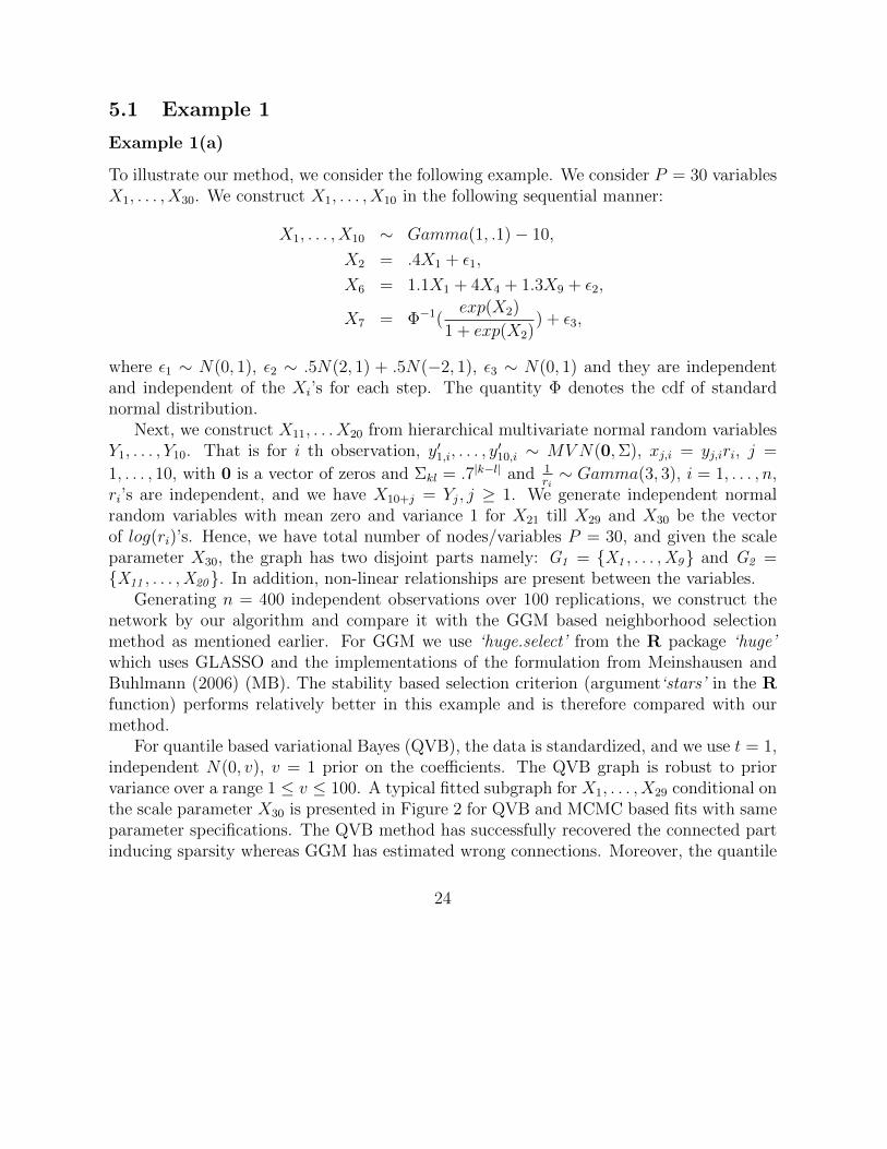
To illustrate our method, we consider the following example. We consider P = 30 variablesX1, . . . , X30. We construct X1, . . . , X10 in the following sequential manner:

X1, . . . , X10 ∼ Gamma(1, .1)− 10,

X2 = .4X1 + ε1,

X6 = 1.1X1 + 4X4 + 1.3X9 + ε2,

X7 = Φ−1(exp(X2)

1 + exp(X2)) + ε3,

where ε1 ∼ N(0, 1), ε2 ∼ .5N(2, 1) + .5N(−2, 1), ε3 ∼ N(0, 1) and they are independentand independent of the Xi’s for each step. The quantity Φ denotes the cdf of standardnormal distribution.

Next, we construct X11, . . . X20 from hierarchical multivariate normal random variablesY1, . . . , Y10. That is for i th observation, y′1,i, . . . , y

′10,i ∼ MVN(0,Σ), xj,i = yj,iri, j =

1, . . . , 10, with 0 is a vector of zeros and Σkl = .7|k−l| and 1ri∼ Gamma(3, 3), i = 1, . . . , n,

ri’s are independent, and we have X10+j = Yj, j ≥ 1. We generate independent normalrandom variables with mean zero and variance 1 for X21 till X29 and X30 be the vectorof log(ri)’s. Hence, we have total number of nodes/variables P = 30, and given the scaleparameter X30, the graph has two disjoint parts namely: G1 = X1 , . . . ,X9 and G2 =X11 , . . . ,X20. In addition, non-linear relationships are present between the variables.

Generating n = 400 independent observations over 100 replications, we construct thenetwork by our algorithm and compare it with the GGM based neighborhood selectionmethod as mentioned earlier. For GGM we use ‘huge.select’ from the R package ‘huge’which uses GLASSO and the implementations of the formulation from Meinshausen andBuhlmann (2006) (MB). The stability based selection criterion (argument‘stars’ in the Rfunction) performs relatively better in this example and is therefore compared with ourmethod.

For quantile based variational Bayes (QVB), the data is standardized, and we use t = 1,independent N(0, v), v = 1 prior on the coefficients. The QVB graph is robust to priorvariance over a range 1 ≤ v ≤ 100. A typical fitted subgraph for X1, . . . , X29 conditional onthe scale parameter X30 is presented in Figure 2 for QVB and MCMC based fits with sameparameter specifications. The QVB method has successfully recovered the connected partinducing sparsity whereas GGM has estimated wrong connections. Moreover, the quantile

24

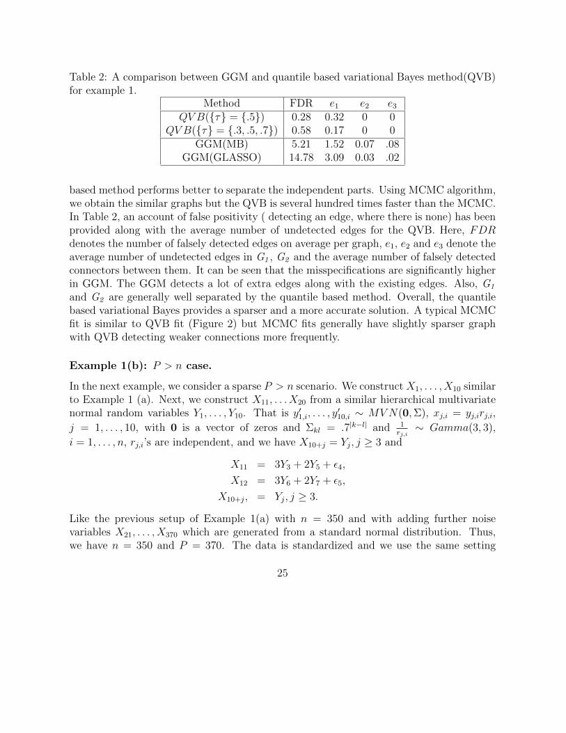
Table 2: A comparison between GGM and quantile based variational Bayes method(QVB)for example 1.

Method FDR e1 e2 e3

QV B(τ = .5) 0.28 0.32 0 0QV B(τ = .3, .5, .7) 0.58 0.17 0 0

GGM(MB) 5.21 1.52 0.07 .08GGM(GLASSO) 14.78 3.09 0.03 .02

based method performs better to separate the independent parts. Using MCMC algorithm,we obtain the similar graphs but the QVB is several hundred times faster than the MCMC.In Table 2, an account of false positivity ( detecting an edge, where there is none) has beenprovided along with the average number of undetected edges for the QVB. Here, FDRdenotes the number of falsely detected edges on average per graph, e1, e2 and e3 denote theaverage number of undetected edges in G1 , G2 and the average number of falsely detectedconnectors between them. It can be seen that the misspecifications are significantly higherin GGM. The GGM detects a lot of extra edges along with the existing edges. Also, G1

and G2 are generally well separated by the quantile based method. Overall, the quantilebased variational Bayes provides a sparser and a more accurate solution. A typical MCMCfit is similar to QVB fit (Figure 2) but MCMC fits generally have slightly sparser graphwith QVB detecting weaker connections more frequently.

Example 1(b): P > n case.

In the next example, we consider a sparse P > n scenario. We construct X1, . . . , X10 similarto Example 1 (a). Next, we construct X11, . . . X20 from a similar hierarchical multivariatenormal random variables Y1, . . . , Y10. That is y′1,i, . . . , y

′10,i ∼ MVN(0,Σ), xj,i = yj,irj,i,

j = 1, . . . , 10, with 0 is a vector of zeros and Σkl = .7|k−l| and 1rj,i∼ Gamma(3, 3),

i = 1, . . . , n, rj,i’s are independent, and we have X10+j = Yj, j ≥ 3 and

X11 = 3Y3 + 2Y5 + ε4,

X12 = 3Y6 + 2Y7 + ε5,

X10+j, = Yj, j ≥ 3.

Like the previous setup of Example 1(a) with n = 350 and with adding further noisevariables X21, . . . , X370 which are generated from a standard normal distribution. Thus,we have n = 350 and P = 370. The data is standardized and we use the same setting

25

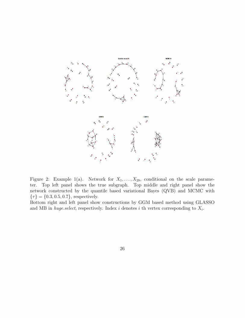
Figure 2: Example 1(a). Network for X1, . . . , X29, conditional on the scale parame-ter. Top left panel shows the true subgraph. Top middle and right panel show thenetwork constructed by the quantile based variational Bayes (QVB) and MCMC withτ = 0.3, 0.5, 0.7, respectively.Bottom right and left panel show constructions by GGM based method using GLASSOand MB in huge.select, respectively. Index i denotes i th vertex corresponding to Xi.

26

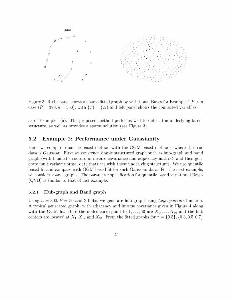
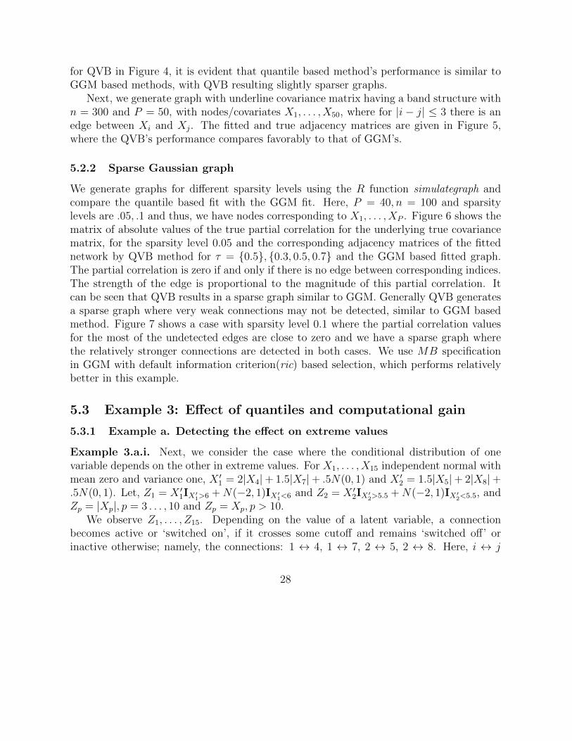
Figure 3: Right panel shows a sparse fitted graph by variational Bayes for Example 1 P > ncase (P = 370, n = 350), with τ = .5 and left panel shows the connected variables.

as of Example 1(a). The proposed method performs well to detect the underlying latentstructure, as well as provides a sparse solution (see Figure 3).

5.2 Example 2: Performance under Gaussianity

Here, we compare quantile based method with the GGM based methods, where the truedata is Gaussian. First we construct simple structured graph such as hub-graph and bandgraph (with banded structure in inverse covariance and adjacency matrix), and then gen-erate multivariate normal data matrices with those underlying structures. We use quantilebased fit and compare with GGM based fit for such Gaussian data. For the next example,we consider sparse graphs. The parameter specification for quantile based variational Bayes(QVB) is similar to that of last example.

5.2.1 Hub-graph and Band graph

Using n = 300, P = 50 and 3 hubs, we generate hub graph using huge.generate function.A typical generated graph, with adjacency and inverse covariance given in Figure 4 alongwith the GGM fit. Here the nodes correspond to 1, . . . , 50 are X1, . . . , X50 and the hubcenters are located at X1, X17 and X34. From the fitted graphs for τ = 0.5, 0.3, 0.5, 0.7

27

for QVB in Figure 4, it is evident that quantile based method’s performance is similar toGGM based methods, with QVB resulting slightly sparser graphs.

Next, we generate graph with underline covariance matrix having a band structure withn = 300 and P = 50, with nodes/covariates X1, . . . , X50, where for |i − j| ≤ 3 there is anedge between Xi and Xj. The fitted and true adjacency matrices are given in Figure 5,where the QVB’s performance compares favorably to that of GGM’s.

5.2.2 Sparse Gaussian graph

We generate graphs for different sparsity levels using the R function simulategraph andcompare the quantile based fit with the GGM fit. Here, P = 40, n = 100 and sparsitylevels are .05, .1 and thus, we have nodes corresponding to X1, . . . , XP . Figure 6 shows thematrix of absolute values of the true partial correlation for the underlying true covariancematrix, for the sparsity level 0.05 and the corresponding adjacency matrices of the fittednetwork by QVB method for τ = 0.5, 0.3, 0.5, 0.7 and the GGM based fitted graph.The partial correlation is zero if and only if there is no edge between corresponding indices.The strength of the edge is proportional to the magnitude of this partial correlation. Itcan be seen that QVB results in a sparse graph similar to GGM. Generally QVB generatesa sparse graph where very weak connections may not be detected, similar to GGM basedmethod. Figure 7 shows a case with sparsity level 0.1 where the partial correlation valuesfor the most of the undetected edges are close to zero and we have a sparse graph wherethe relatively stronger connections are detected in both cases. We use MB specificationin GGM with default information criterion(ric) based selection, which performs relativelybetter in this example.

5.3 Example 3: Effect of quantiles and computational gain

5.3.1 Example a. Detecting the effect on extreme values

Example 3.a.i. Next, we consider the case where the conditional distribution of onevariable depends on the other in extreme values. For X1, . . . , X15 independent normal withmean zero and variance one, X ′1 = 2|X4|+ 1.5|X7|+ .5N(0, 1) and X ′2 = 1.5|X5|+ 2|X8|+.5N(0, 1). Let, Z1 = X ′1IX′1>6 +N(−2, 1)IX′1<6 and Z2 = X ′2IX′2>5.5 +N(−2, 1)IX′2<5.5, andZp = |Xp|, p = 3 . . . , 10 and Zp = Xp, p > 10.

We observe Z1, . . . , Z15. Depending on the value of a latent variable, a connectionbecomes active or ‘switched on’, if it crosses some cutoff and remains ‘switched off’ orinactive otherwise; namely, the connections: 1 ↔ 4, 1 ↔ 7, 2 ↔ 5, 2 ↔ 8. Here, i ↔ j

28

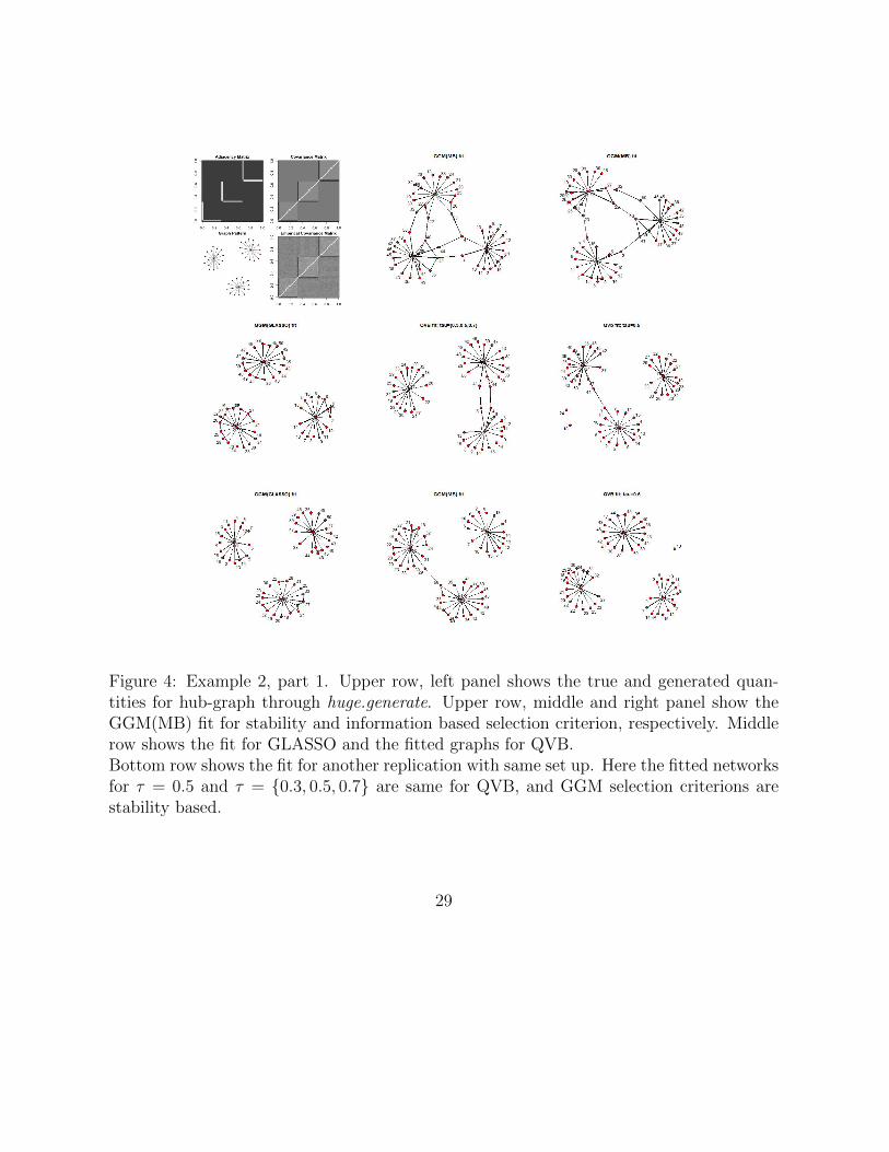
Figure 4: Example 2, part 1. Upper row, left panel shows the true and generated quan-tities for hub-graph through huge.generate. Upper row, middle and right panel show theGGM(MB) fit for stability and information based selection criterion, respectively. Middlerow shows the fit for GLASSO and the fitted graphs for QVB.Bottom row shows the fit for another replication with same set up. Here the fitted networksfor τ = 0.5 and τ = 0.3, 0.5, 0.7 are same for QVB, and GGM selection criterions arestability based.

29

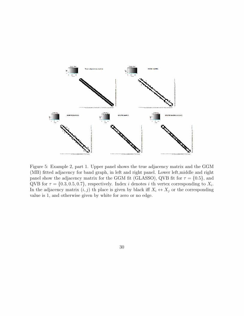
Figure 5: Example 2, part 1. Upper panel shows the true adjacency matrix and the GGM(MB) fitted adjacency for band graph, in left and right panel. Lower left,middle and rightpanel show the adjacency matrix for the GGM fit (GLASSO), QVB fit for τ = 0.5, andQVB for τ = 0.3, 0.5, 0.7, respectively. Index i denotes i th vertex corresponding to Xi.In the adjacency matrix (i, j) th place is given by black iff Xi ↔ Xj or the correspondingvalue is 1, and otherwise given by white for zero or no edge.

30

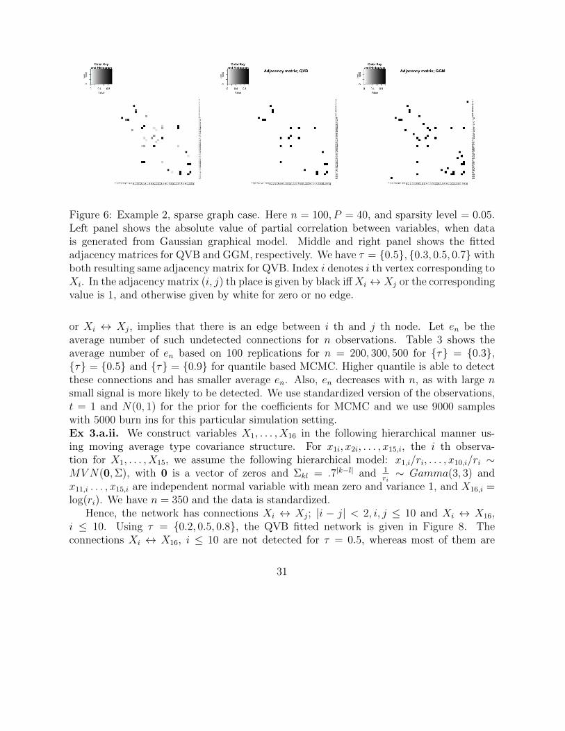
Figure 6: Example 2, sparse graph case. Here n = 100, P = 40, and sparsity level = 0.05.Left panel shows the absolute value of partial correlation between variables, when datais generated from Gaussian graphical model. Middle and right panel shows the fittedadjacency matrices for QVB and GGM, respectively. We have τ = 0.5, 0.3, 0.5, 0.7 withboth resulting same adjacency matrix for QVB. Index i denotes i th vertex corresponding toXi. In the adjacency matrix (i, j) th place is given by black iffXi ↔ Xj or the correspondingvalue is 1, and otherwise given by white for zero or no edge.

or Xi ↔ Xj, implies that there is an edge between i th and j th node. Let en be theaverage number of such undetected connections for n observations. Table 3 shows theaverage number of en based on 100 replications for n = 200, 300, 500 for τ = 0.3,τ = 0.5 and τ = 0.9 for quantile based MCMC. Higher quantile is able to detectthese connections and has smaller average en. Also, en decreases with n, as with large nsmall signal is more likely to be detected. We use standardized version of the observations,t = 1 and N(0, 1) for the prior for the coefficients for MCMC and we use 9000 sampleswith 5000 burn ins for this particular simulation setting.Ex 3.a.ii. We construct variables X1, . . . , X16 in the following hierarchical manner us-ing moving average type covariance structure. For x1i, x2i, . . . , x15,i, the i th observa-tion for X1, . . . , X15, we assume the following hierarchical model: x1,i/ri, . . . , x10,i/ri ∼MVN(0,Σ), with 0 is a vector of zeros and Σkl = .7|k−l| and 1

ri∼ Gamma(3, 3) and

x11,i . . . , x15,i are independent normal variable with mean zero and variance 1, and X16,i =log(ri). We have n = 350 and the data is standardized.

Hence, the network has connections Xi ↔ Xj; |i − j| < 2, i, j ≤ 10 and Xi ↔ X16,i ≤ 10. Using τ = 0.2, 0.5, 0.8, the QVB fitted network is given in Figure 8. Theconnections Xi ↔ X16, i ≤ 10 are not detected for τ = 0.5, whereas most of them are

31

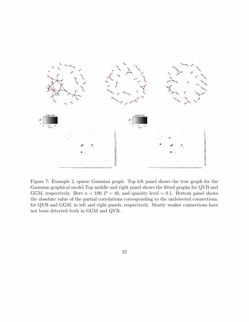
Figure 7: Example 2, sparse Gaussian graph. Top left panel shows the true graph for theGaussian graphical model.Top middle and right panel shows the fitted graphs for QVB andGGM, respectively. Here n = 100, P = 40, and sparsity level = 0.1. Bottom panel showsthe absolute value of the partial correlations corresponding to the undetected connections,for QVB and GGM, in left and right panels, respectively. Mostly weaker connections havenot been detected both in GGM and QVB.

32

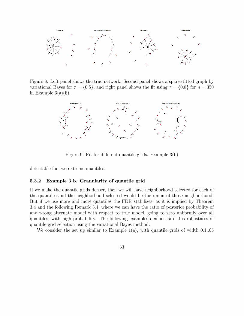
Figure 8: Left panel shows the true network. Second panel shows a sparse fitted graph byvariational Bayes for τ = 0.5, and right panel shows the fit using τ = 0.8 for n = 350in Example 3(a)(ii).

Figure 9: Fit for different quantile grids. Example 3(b)

detectable for two extreme quantiles.

5.3.2 Example 3 b. Granularity of quantile grid

If we make the quantile grids denser, then we will have neighborhood selected for each ofthe quantiles and the neighborhood selected would be the union of those neighborhood.But if we use more and more quantiles the FDR stabilizes, as it is implied by Theorem3.4 and the following Remark 3.4, where we can have the ratio of posterior probability ofany wrong alternate model with respect to true model, going to zero uniformly over allquantiles, with high probability. The following examples demonstrate this robustness ofquantile-grid selection using the variational Bayes method.

We consider the set up similar to Example 1(a), with quantile grids of width 0.1,.05

33

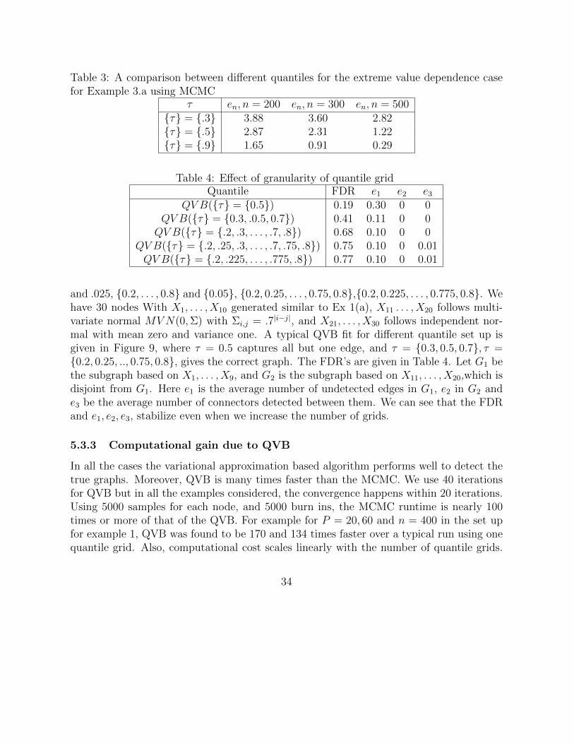
Table 3: A comparison between different quantiles for the extreme value dependence casefor Example 3.a using MCMC

τ en, n = 200 en, n = 300 en, n = 500τ = .3 3.88 3.60 2.82τ = .5 2.87 2.31 1.22τ = .9 1.65 0.91 0.29

Table 4: Effect of granularity of quantile gridQuantile FDR e1 e2 e3

QV B(τ = 0.5) 0.19 0.30 0 0QV B(τ = 0.3, .0.5, 0.7) 0.41 0.11 0 0QV B(τ = .2, .3, . . . , .7, .8) 0.68 0.10 0 0

QV B(τ = .2, .25, .3, . . . , .7, .75, .8) 0.75 0.10 0 0.01QV B(τ = .2, .225, . . . , .775, .8) 0.77 0.10 0 0.01

and .025, 0.2, . . . , 0.8 and 0.05, 0.2, 0.25, . . . , 0.75, 0.8,0.2, 0.225, . . . , 0.775, 0.8. Wehave 30 nodes With X1, . . . , X10 generated similar to Ex 1(a), X11 . . . , X20 follows multi-variate normal MVN(0,Σ) with Σi,j = .7|i−j|, and X21, . . . , X30 follows independent nor-mal with mean zero and variance one. A typical QVB fit for different quantile set up isgiven in Figure 9, where τ = 0.5 captures all but one edge, and τ = 0.3, 0.5, 0.7, τ =0.2, 0.25, .., 0.75, 0.8, gives the correct graph. The FDR’s are given in Table 4. Let G1 bethe subgraph based on X1, . . . , X9, and G2 is the subgraph based on X11, . . . , X20,which isdisjoint from G1. Here e1 is the average number of undetected edges in G1, e2 in G2 ande3 be the average number of connectors detected between them. We can see that the FDRand e1, e2, e3, stabilize even when we increase the number of grids.

5.3.3 Computational gain due to QVB

In all the cases the variational approximation based algorithm performs well to detect thetrue graphs. Moreover, QVB is many times faster than the MCMC. We use 40 iterationsfor QVB but in all the examples considered, the convergence happens within 20 iterations.Using 5000 samples for each node, and 5000 burn ins, the MCMC runtime is nearly 100times or more of that of the QVB. For example for P = 20, 60 and n = 400 in the set upfor example 1, QVB was found to be 170 and 134 times faster over a typical run using onequantile grid. Also, computational cost scales linearly with the number of quantile grids.

34

Our computation is parallelizable over nodes and the grids of quantiles, though we do notimplement it here.

6 Protein network

The Cancer Genome Atlas (TCGA) is a source of molecular profiles for many differenttumor types. Functional protein analysis by reverse-phase protein arrays (RPPA) is in-cluded in TCGA and looking at the proteomic characterization the signaling network canbe established.

Proteomic data generated by RPPA across > 8000 patient tumors obtained from TCGAincludes many different cancer types. We consider lung squamous cell carcinoma (LUSC)data set. The data set considered, has n = 121 observations with P = 174 high-qualityantibodies. The antibodies encompass major functional and signaling pathways relevantto human cancer and a relevant network gives us their interconnection subject to LUSC. Acomprehensive analysis of similar network can be found in Akbani et al. (2014) for variouscancers, where the EGFR family along with MAPK and MEK lineage was found to bedominant determinant of signaling, where for LUSC it was mainly EGFR.

We use our quantile based variational approach with τl = .1, .2, .3, . . . , .7, .8, .9 anda normal prior on β (independent N(0, 1)). Overall, the QVB graph is robust to thisprior variance(v) selection in the range v = [1, 100] with very few of the edges/weakerconnections may be missing for a relatively higher variance. The data is standardized andwe use t = 1. The graphical LASSO method cannot select a sparse (using huge.select)network both using criterion ‘MB’ or ‘GLASSO’ and using criterions for tuning parameterselection. Choosing the penalization by direct cross validation in GLASSO in Akbani etal. (2014), the network has been generated and it reports the important connections.

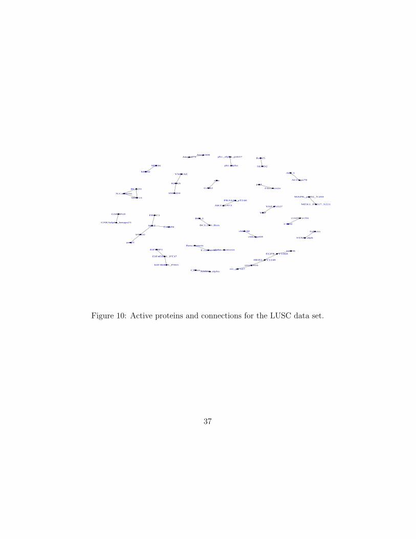
The network and the connection tables with variable index can be found in Figure10 and Table 5. The type of the connection (positive/negative) is also provided. Wecan say that one variable effects other variable positively (negatively), conclusively, if thecoefficients in the corresponding quantile regression is greater (less) than zero for at leastone quantile, and greater (less) than equal to zero for other quantiles. A network ofprotein was established for different cancer types in Akbani et al. (2014), where importantconnections were established. We compare our network for the LUSC network from Akbaniet al. where we find some of the known established connections are detected and also someconnection not mentioned in Akbani et al. have been detected. Though we refrain frommaking any inferential claim about the new connections, some further study may be helpful

35

for possibly new biological insight.In our fitted network, the strong EGFR/HER2 connections are detected as seen in Ak-

bani et al. (2014). The connection between EGFRpY 1068 and HER2p Y 1248 is detectedwhich are known to cross react. The connection betweenE.Cadherin and alph/beta.Cateninis detected as expected. Unlike Akbani et al., pAkt and Pras40 are found to be connectedin LUSC. This connection was reported for few other cancer types. Also, MEK is activeand connected to PMAPK. EGFR is known to be active in lung cancer and mutationof MAPK , MEK are known to be present for various cancers (see Yatabe et al. (2008),Hilger et al.(2002) ). Few connections, such as the new negative connection between p85and claudin7, mentioned in Akbani et al. (2014) are not detected in this current set up.

We have detected some new connections not given in Akbani et al. for LUSC data set,such as between SNAI2 and PARP1. Here, SNAI2 is a DNA-transcriptional repressorand PARP1 modulates transcription.

Proteins, casp8 and ERCC1 are found to be connected with MET , which are notgiven in AKbani et al. casp8 performs protein metabolism and ERCC1 is related tostructure specific DNA repairing and known to be important in lung cancer treatment(Ryu et. al. (2014)). They both are connected to growth factor receptor MET . Thedetected connections between KRAS and smad4, YWHAE and KRAS are not given inthe network from Akbani et al. for LUSC data set and need further study.

36

MSH6

MSH2

Aktpt308Aktps473

ACC1

ACC_ps79

Beta.cantein

E.cadherin

SNAI2

parp1

ccnd1.cyclin

CD20

srcpY416

src_pY527

GSK3alpha_betaps21

GSK3Ps9

pai1

Fibrocentin

PRAS40_pT246

AKT_ps473

chk2_pt68

chk2.M Tuberin

STAT5.alph

YAP_Ps127

YAP

AMPK_alphaCDK1

EIF4EBP1_PT37

EIF4EBP1_PS65

alpha_cantenin

ckit

GAB2

HER2_PY1248

EGFR_PY1068

METCASP8

ERCC1

BCL2

BCL2l11.Bim

KRAS

YWHAE

SMAD4

MAPK_pt202_Y204

MEK1_PS217_S221

pkc_alpha_ps657

pkc.alpha

EGFREiF4BP1

Rab25

SETD2

N.Cadherin

MRE11

BCL2l1

Figure 10: Active proteins and connections for the LUSC data set.

37

Table 5: Connections and corresponding nodes in LUSC data setProteins Sign

MSH6↔MSH2 +AktPT308↔ AktPS473 +

ACC1↔ ACC +beta.cantenin↔ E.Cadherin +

SNAI2↔ PARP1 +CCND1.Cyclin↔ CD20 +

SrcpY 416↔ Src +GSK3.alpha.beta.pS21↔ GSk3pS9 +

Pai1↔ Fibrocentin +PRAS40 pT246↔ Akt pS473 +

Chk2 pT68↔ chk2.M +Tuberin↔ STAT5.alpha +Y AP PS127↔ Y AP +

AMPK alpha↔ CDK1 +AMPK PT172↔ AMPK alph +EIF4EBP1 pT37↔ EIF4EBP1 +

EIF4EBP1 pT37↔ EIF4EBP1 PS65 +alpha.Catenin↔ E.Cadherin +

cKit↔ GAB2 +HER2 pY 1248↔ EGFR PY 1068 +HER2 pY 1248↔ Src PY 416 +

MET ↔ SNAI2 +MET ↔ CASP8 +ERCC1↔MET +BCL2↔ Bim +

KRAS ↔ YWHAE +KRAS ↔ Smad4 +

MAPK pT202 Y 204↔MEK1 pS217 S221 +PKC.alpha pS657↔ PKC.alpha +

EGFR↔ EGFRpY 1068 +Rab25↔ SETD2 +

N.Cadherin↔ BCL2 +N.Cadherin↔MRE11 +

38

7 Discussion

The proposed approach offers a robust, non-Gaussian model as well as easily implementablealgorithms for sparse graphical models. Even with large values of P and relatively smallervalue of n, it is possible to detect underlying connections as shown in example 1 and inthe analysis of the LUSC data set. In the protein network construction, we are able toestablish the known signaling network with some newly discovered connections, which needto be validated.

In this development, we prove the density estimation and neighborhood selection con-sistency and posterior concentration rate under both the true model and the misspecifiedmodel. Under misspecified model the posterior concentration occurs around the minimumKL distance point from the true density and the set of proposed densities. From simulationexamples where we do not assume any density structure in the data generating model, theproposed method performs well. In future, we will further investigate the model selectionproperties for each node and related convergence rate.

Acknowledgment

Research reported in this publication was partially supported by National Cancer Insti-tute of the National Institutes of Health under award number R01CA194391, NSF grantsnumbers NSF CCF-1934904, NSF IIS-1741173.

39

8 Appendix

Proof of the theoretical results

Proof of Theorem 3.1:

The sketch of the proof is following. At first we construct the KL neighborhood and showthat it has sufficient prior probability. The sieve is constructed thereon and outside thesieve the prior probability is decreased exponentially. The construction from Jiang (2007)can be used as long as an equivalent KL ball around the true density can be constructedunder the quantile model.

First, we show our calculation for the neighborhood construction of k th node. Leth∗l = x′β∗(−k)

l, h∗1,l = x′β∗(−k)

γn,l,h∗2,l = x′β∗(−k)

γcn,l. Here, coefficient vector with subscript γn

denotes the coefficient is set to be zero if the corresponding variable is not in γn. Similarly,it is defined for the subscript γcn. Also, x denotes a generic row of X = X−k

∗.

In model γn, let H be the set of β(−k)

l’s such that β

(−k)j,l ∈ (β∗j,l

(−k)± η ε2n

rn) for j 6= k ∈ γn,

where |γn| = rn, such that ∆lk(rn) is minimized. Let hl = x′β(−k)

γ,lthen for β(−k)

lin H, we

have

L(f) = |logf(xk, h∗l )

f(xk, hl)| = |log f(xk, h

∗)

f(xk, h∗1,l)

f(xk, h∗1,l)

f(xk, hl)|

≤ t∆lk(rn)

∑j /∈γn

|Xj|+∑j∈γn

tηε2nrn|Xj|,

where f(xk, h) ∝ τ(1−τ)exp(−tρτ (xk−h)). This step follows from the Lemma 1 of Sriramet al. (2013).

Therefore, ∫L(f)f ∗(xk| − k)f ∗(xi 6=k)dx ≤ tM∗(pn∆l

k(rn) + ηε2n) < ε2n

for some appropriately chosen η (by A7). Hence, H lies in the ε2n KL neighborhood.For normal prior on the coefficient, Π(H) ≥ e−cnε

2n and Π(γ = γn) > exp(−cnε2n) for

any c > 0 for large n, similar to Jiang(2007). Therefore, they provide sufficient prior masson small KL neighborhood around the true density.

40

Let Pn be the set such that regression coefficients lies in [−Cn, Cn] and rn is the maxi-

mum model size. For δ = η ε2n

rncovering each of the coefficients by δ radius l∞ balls, in those

balls we have Hellinger distance less than ε2n. Hence, we have the total Hellinger coveringnumber of Pn as N(εn) ≤

∑rnr=0 p

rn(2Cn

2δ+ 1)r ≤ (rn + 1)(pn(Cn

δ+ 1))rn (see Jiang; 2005,

2007).This step follows as d2(p, q) ≤ KL(p, q), where d is the Hellinger metric defined in

section 3 and KL is the Kullback-Leibler distance. Note that, log(N(εn)) = O(rn(log(Cn)+log(pn) + log(1/ε2n))).

We have from A1, A2, using Cn as a large power (greater than one) of n, from Jiang(2005), or any K1 > 0, for large n

log(N(εn), Pn) ≺ nε2n,

Π(P cn) ≤ e−K1nε2n .

Therefore, Theorem 3.1 follows from verification of conditions for Theorems 5, 6 andProof of Theorem 3, from Jiang (2005) or Proposition 1 from Jiang (2007).

From Proposition 1 part (i) from Jiang (2007), P ∗[Π(hk > εn|Dn) > e−c′1nε

2n ] → 0 for

some c′1 > 0.

Beta-Binomial Prior

We have shown the result for Ij,l ∼ Bernouli(πn) with rn = pnπn, rn satisfying A1–A7. Weuse the same rn for Beta-Binomial prior calculation. For γn with model size rn, constructedas in proof of Theorem 3.1, we show that the prior mass condition holds.

For Beta-Binomial prior on Ij,l, we have for a1 = b1 = 1,

Π(γ = γn) ≥((pn + 1)

(pnrn

))−1.

From A1, Π(γ = γn) > (pn + 1)−(rn+1) > exp(−cnε2n) for any c > 0 for large n. Therefore,the condition on prior mass holds. Hence, from the earlier proof, Theorem 3.1 follows.

Proof of Theorem 3.2

We prove this part for fixed tl = t, and without loss of generality t is assumed to be1. For Theorem 3.2 and 3.3 we first prove under the assumption of bounded covariatewith |Xk| < M for a simplified proof. Later, we relax the condition to accommodate sub

41

exponential tail bound. To show the concentration of fl,k,−k under Πl(·), around f ∗l,k,−k theclosest point in conditional quantile based likelihood for τl, we drop the suffix l in fl,k,−k(·),βl, δ∗k,l and Πl(·) for convenience and show for one general quantile.

We have

Π(KL(f 0k,−kf

0−k, fk,−k(β

(−k))f 0−k) > δ + δ∗k|.) =

∫Kcδfnk,−k(β

(−k)

γ)Π(β, γ)d(β, γ)∫

fnk,−k(β(−k)

γ)Π(β, γ)d(β, γ)

≤

∫Kcδfnk,−k(β

(−k)

γ)Π(β, γ)d(β, γ)∫

vδ′,γ0fnk,−k(β

(−k)

γ)Π(β, γ)dβ

=Nn

Dn

. (11)

Here, γ0 the vector of 0 and 1 corresponding to the active set (i.e present in the model)of covariates for k th node for the model with the KL distance δ∗k, and let |γ0| = M ′

0, the

cardinality of the active set and vδ′,γ0 be the set with γ0 active and where ‖β(−k)

γ0−β

(−k)

γ0‖∞ <

δ′. Here, Kcδ denotes the set of densities where the KL distance from the f 0

k,−kf0−k is more

than δ+ δ∗k. On Kcδ , Ef0(log

f∗k,−kfk,−k

) = KL(f 0k,−kf

0−k, fk,−kf

0−k)−KL(f 0

k,−kf0−k, f

∗k,−kf

0−k) > δ.

Also, n in the density fnk,−k denotes the likelihood based on n observations. We divideNn and Dn by fn∗k,−k which is likelihood based on n observations under this minimum KLdistance model at k th node for τl.

Under Beta-Binomial prior Π(γ = γn) >((pn + 1)

(pnM ′0

))−1> e−M0log(pn+1). Note that

if the difference between coefficient vectors is δ∗ in supremum norm, then the differencebetween corresponding log likelihood is at most MM0δ

∗, by B1 and lemma 1(b) from Sriramet al (2013), if we assume M > 1 without loss of generality.

Therefore, for the denominator, we have encδ′ Dnfn∗k,−k

> e−M0log(pn+1)Π(vδ′,γ0) en(c−M(M0+1))δ′ >

1 if c > M(M0 + 1), for large n.We split the numerator in two parts. First part contains the part where each of the

entry of β(−k) lies in [−Kc−mβ, Kc +mβ] a compact set with mβ = ‖β(−k)‖∞ and Kc > 0.

We denote the set by S and its compliment by Sc. Also, let msβ = supk‖β

(−k)‖∞. For

notational convenience, we will drop the index k from the coefficient.

42

Calculation on S:

For any of the at most cn ≤ 2M0(pn−1M0

)many covariate combinations ( a conservative bound)

for the kth node, we show the part in the S decreases to zero exponentially fast. Note that(pn−1M0

)< pM0

n . For any covariate combination, we break the M0 dimensional model space

in S in (MM0)−1δ′′

width M0 dimensional squares.Let, Jn(δ

′′) be the number of squares and for density fk,−k associated with each nodal

point of the (MM0)−1δ′′

width grids, we havefnk,−kfn∗k,−k

≤ e−.5nδ for large n with probability

one, as n−1logfnk,−kfn∗k,−k

→ Ef0(logfk,−kf∗k,−k

) < −δ.

Also, over all possible covariate combinations: P (fnk,−kfn∗k,−k

> e−.5nδ, infinitely often (i.o)) =

P (n−1logfnk,−kfn∗k,−k

> −.5δ, i.o) ≤ P (n−1logfnk,−kfn∗k,−k−Ef0(log

fk,−kf∗k,−k

) > .5δ, i.o) ≤ 2M0lim∑∞

n pM0n e

−cnδ2

t2s

→ 0, by Hoeffding inequality and Borel-Cantelli lemma using B4. Here, ts = M0(M +

1)(Kc +msβ) and c > 0 is a generic constant and |log fk,−k

f∗k,−k| < 2ts.

For any point β = β(−k) and its nearest grid point βgrid

, we havefnk,−k(β)

fnk,−k(βgrid

)≤ enδ

′′(an

application of Lemma 1(b), Sriram et al.,2013).Choosing δ

′′less than .25δ, for large n we have for all the combinations of γ′ on S,

pr.,n =∑

γ′

∫S,γ′

fnk,−kfn∗k,−k

Π(.) ≤ eM0logpnJn(δ′′)e−nd1δ where d1 > 0 is a constant depending

upon δ′′

. Also, logpn ≺ n. Therefore, pr.,n < e−.5nd1δ almost surely.

Calculation on Sc:

Next, we look at Sc. Let, cτ = minlτl, 1 − τl. On Sc, at least one βi,l is outside

[−Kc −mβ, Kc +mβ]. Without loss of generality we assume βi,l − βi,l’s have same sign as

β0,l − β0,l (otherwise we change X ′i = −Xi and work with the reflected variable). Withoutloss of generality, we denote the covariate X ′i, i 6= k encompassing both reflected and nonreflected scenarios. As there are only finitely many orderings, it is sufficient to consideronly one such case and prove in that case. Furthermore without loss of generality, thevariables are assumed to be centered.

First, we consider the case when β0,l > β0,l. The case β0,l < β0,l follows identically. Weshow our calculation for τl, y = Xk and the covariates X ′1, X

′2, when M0 = 2. For general

M0, it follows similarly. Let bi,l = β0,l − β0,l + (β1,l − β1,l)x′1,i + (β2,l − β2,l)x

′2,i. Note that if

x′1,i, x′2,i > ε > 0, then bi,l > 0.

43

Let

δi,l = ρτl(yi − β0,l − β1,lx′1,i − β2,lx

′2,i)− ρτl(yi − β0,l − β1,lx

′1,i − β2,lx

′2,i).

Then from Lemma 1 and Lemma 5 from Sriram et al. (2013)

δi,l ≥ cτ εKcIx′1,i>ε,x′2,i>ε − 2|yi − β0,l − β1,lx′1,i − β2,lx

′2,i|.

Let, Aiε = x′1,i > ε, x′2,i > ε and Biε = x′1,i < −ε, x′2,i < −ε. The previous step

follows from the proof of the Lemma 1 in Sriram et al. (2013) by writing down the loss

function explicitly and from the fact that bi,l = µ(2)i,l − µ

(1)i,l > 0 on Aiε, where µ

(1)i,l =

β0,l + β1,lx′1,i + β2,lx

′2,i and µ

(2)i,l = β0,l + β1,lx

′1,i + β2,lx

′2,i. Considering the ordering of

yi, µ(1)i,l , µ

(2)i,l , such as yi ≤ µ

(1)i,l ≤ µ

(2)i,l ; µ

(1)i,l ≤ yi ≤ µ

(2)i,l and so on, the above claim can be

verified.Let minE(IAiε), E(IBiε) = aε > 0 (by B3, choosing appropriate ε > 0) and ri =

|yi−β0,l−β1,lx′1,i−β2,lx

′2,i| and E(ri) ≤ ε′, over all nodes and all possible model combination

of size at most M0, at each node (follows from uniformly bounded ‖β(−k)‖∞ and uniformly

bounded second moments).

Establishing bound on the average of the indicators and ri

By Hoeffding bound P (∑n

i=1 n−1(IAiε) <

aε2

) < e−2na2ε4 and similar bound holds for Bi

ε.

Similarly, P (n−1∑n

i=1(ri) > 2ε′) < e−c2n(ε′)2 for some constant c2 as Xk’s are bounded.

Hence by Borel-Cantelli lemma, the probabilityn−1

∑ni=1(I

Aiε)

n−1∑ni=1 ri

< aε4ε′

infinitely often is less

than

limN→∞

∞∑n=N

pM0n (e−c2n(ε′)2 + e−2n

a2ε4 )→ 0

by B4.

Therefore for all the possible at most M0 neighbors, we have,n−1

∑ni=1(I

Aiε)

n−1∑ni=1 ri

> d0 > 0 for

some d0 for all but finitely many cases, with probability 1. The calculation holds for eachquantile.

Also, lim∑∞

n=N pnpM0n (e−c2n(ε′)2+e−2n

a2ε4 )→ 0 similarly. Therefore, this result holds over

the union over all the vertices /nodes of the graph, over all possible model combination ofmaximum size M0 − 1.

44

Hence choosing Kc large enough, on Sc we have logfnk,−k()−logfn∗k,−k = −∑

i δi,l ≤ −nu0,where u0 > 0, for large n, almost surely.

Therefore choosing δ′ < minu0,.5d1δ2M(M0+1)

, from (11) LHS goes to zero almost surely, as

encδ′ Nnfn∗k,−k

→ 0, by choosing c = 1.5M(M0 + 1).

Proof of Theorem 3.3

This proof follows similar construction of S and Sc from the previous proof of Theorem3.2. Here we show for bounded Xk’s first.On S

For any of the at most cn ≤ 2M0(pn−1M0

)many covariate combinations for the kth node, we

show the part in the S decreases to zero exponentially fast. We break the M0 dimensionalmodel space in (MM0)−1δ

′′width M0 dimensional squares.

Let, Jn(δ′′)be the number of squares and for each nodal point we show

fnk,−kfn∗k,−k

≤ e−2nε2n

almost surely. This step follows from the following application of Hoeffding inequality.Note that, Jn(δ

′′) = O(( 1

δ′′)M0).

Showingfnk,−kfn∗k,−k

≤ e−nε2n for large n on S

Let, tm = M0(M + 1)(Kc +mβ), ts = M0(M + 1)(Kc +msβ). We have E(n−1log(

fnk,−kfn∗k,−k

)) <

−4ε2n.

Then, P (n−1log(fnk,−kfn∗k,−k

) > −2ε2n, for some grid points) < cM0Jn(δ′′)e−2n

ε4n4t2m . Here, cM0 is

the number of grid points associated with a M0 dimensional grid and |log fk,−kf∗k,−k| < 2tm.

Choosing δ′′

= ε2n , we have P (fnk,−kfn∗k,−k

> e−2nε2n infinitely often) ≤ cM0 lim N→∞∑∞

n=N

Jn(δ′′)e−2n

ε4n4t2m . Now from B6 and B7 we get

∑Jn(δ

′′)e−2n

ε4n4t2m <∞. Therefore using Borel-

Cantelli lemma,fnk,−kfn∗k,−k

≤ e−2nε2n almost surely.

Moreover,∑

n pnpM0n Jn(δ

′′)e−2n

ε4n4t2s < ∞ (by B7). Therefore, this almost surely conver-

gence happens over all possible covariate combinations and over all pn vertices/nodes ofthe graph.

45

For any point β and its nearest grid point βgrid

,we havefnk,−k(β)

fnk,−k(βgrid

)≤ enδ

′′. Therefore

on S, we havefnk,−k(β)

fn∗k,−k≤ e−nε

2n , almost surely.

Combining the parts

Calculation on S:

Choosing, δ′

= .5 ε2nMM0

, we have −logΠ(vδ′,γ0) = O(log 1ε2n

) and encδ′ Dnf∗k,−k

> e−M0logpn

Π(vδ′,γ0)en(c−MM0)δ′ > 1 if c > MM0, for large n, from B6, B7.

Therefore on S, choosing c > MM0 and .5ε2n < cδ′< .75ε2n∫

Kcδ∩S

fnk,−k(βγ)π(β, γ)d(β, γ)∫vδ′,γ0

fnk,−k(βγ)π(β, γ)dβ≤ e−.25nε2n .

On Sc

On Sc, the result from Theorem 3.2 holds and logfk,−k(.) − logf ∗k,−k ≤ −nu0 almostsurely for large n.

Therefore, with n, pn going to infinity, P (Π(KL(f 0k,−kf

0−k, fl,k,−kf

0−k) > δn+δ∗k for some node |.)

goes to zero almost surely.

Relaxing boundedness condition

From B2, using Holder inequality, we have that for any M0 + 1 dimensional linear com-bination of absolute values of Xi’s with bounded coefficient (where coefficient of Xi’s arebounded by 1), denoting the random variable by generic symbol W :

E(eλ(W−E(W ))) ≤ e.5λ2ν∗2 for |λ| < b−1

for some global b, ν∗ < ∞, for all possible such combinations. This is the condition forsub-exponential distribution with parameters (ν∗, b) with ν∗2 = (M0 + 1)ν2.

Showing for linear combinationsThis result follows from the following argument using Holder’s inequality,

E(eλ∑Mi=1 αi(Xi−E(Xi))) ≤ E(e|λ|

∑Mi=1 |αi(Xi−E(Xi))|) ≤ e.5λ2M2ν2

1M ≤ e.5λ

2(M0+1)ν2 .

Then for w1, . . . , wn i.i.d W with mean W , we have P (|W −E(W )| > t′) ≤ 2e− n2t′2

2(n(ν∗)2+nbt′)

(Bernstein-type inequality). Thus, we induce uniform tail bound on the variables/nodesand their linear combinations.

46

Showing Theorem 3.3 for sub-exponential tail bound

From the tail bound result for linear combinations

P (n−1

n∑i=1

(|xij1|+ · · ·+ |xijm|) > KM for some j1, . . . , jm ∈ 1, . . . , pn;m ≤M0 − 1)

≤ pM0n e−c1n (12)

with some c1 > 0, KM = 1.5M0maxE(|Xk|), as b < ∞. Hence, n−1∑n

i=1(|xij1| + · · · +|xijm|) ≤ KM for all but finitely many cases, almost surely by Borel-Cantelli lemma, as∑pM0n e−c1n <∞.We can choose δ′ = .5

KM+1ε2n and for Dn, on vδ′,γ0 we have n−1|logfn∗k,−k − logfnk,−k| ≤

.5(KM+1)

ε2nn−1∑

i

∑j∈γ0 |xij| ≤ .5ε2n as n goes to infinity (using Lemma 1(b), Sriram et al.,

2013). Similarly, for Nn, on S we choose ((KM + 1))−1δ′′ size grids and the conclusion forbounded case holds.

On S the absolute value of the coefficients are bounded by Kmax = Kc +msβ. For linear

combination with bounded coefficient, we assumed sub-exponential distribution. Sameholds for differences of such functions with bounded intercept terms, similarly (withoutloss of generality, we bound the absolute value of coefficients and intercept terms by one,to get the global b, ν∗ in sub exponential formulation, using Holder’s inequality). Weassume global constants b, ν , in the sub-exponential condition, slightly abusing the earliernotation.

Finally, for each of the grid points,

P (n−1(logfnk,−kfn∗k,−k

) > −2ε2n) = P (n−1 1

Kmax

(logfnk,−k − logfn∗k,−k) > −2ε2n

Kmax

)

< e− c2

(Kc+msβ)2nε4n

for some fixed c2 > 0 . This step follows using the sub-exponential property for the quantileloss functions at nodes and their linear combination, as we have shown it for absolute valuethe linear combinations of the covariates earlier, as b, ν are global constants, in the sub-exponential assumption in this case. On Sc the bound on n−1

∑ni=1 ri follows similarly, as

the intercept β0,l and the coefficients are bounded. Hence, the proof of Theorem 3.3 holdsunder relaxed assumptions.

47

Proof of Proposition 2.1

The proof follows trivially from model given in equation 1 from the main manuscript andthe linearity of conditional quantile function.

Proof of Lemma 1

Follows readily from the fact that under C1, if Xj is not connected to Xk then j is notcontained in any N∗l,k, and if Xj ↔ Xk, then from C2, Xj is in some N∗l,k if we choose smallenough quantile grid width.

Proof of Theorem 3.4

Let, M∗l,k be the model for τl at k th node induced by N∗l,k, and M1

k 6= M∗l,k be any competing

model at node k. Let fnl,k,−k,M1(β) = fnl,k,−k,β

M1

be the likelihood under Equation 4, for n

observations for coefficient β = βl, for some model M1, at node k . Then,

Πnl,k(M

1k ,M

∗l,k) ≤ cπ

−s∗+sM1n

∫fnl,k,−k,M1

k(β)π(β)dβ∫

fnl,k,−k,M∗l,k(β)π(β)dβ

= cπ−s∗+sM1n

∫ fnl,k,−k,M1

k

(β)

fnk,−k,β

M∗l,k

π(β)dβ

∫ fnl,k,−k,M∗

l,k(β)π(β)

fnk,−k,β

M∗l,k

dβ

= cπ−s∗+sM1n

NnBF

DnBF

. (13)

Here the suffix l denote the likelihood used corresponds to τl, c < 2M0 is a constant asπn ≤ 0.5 without loss of generality. Let β

M∗l,kor the vector of β0, β1, . . . , βm∗ be the true

values of coefficients that minimizes the expected quantile loss and the KL distance withthe data generating density. Without loss of generality we can choose them to be first m∗

variables. Let s∗ = m∗ be the size of true model for k th node and sM1 = sM1k

be the sizeof the competing model. For convenience we drop the l and writing M∗

k instead of M∗l,k,

we write βM∗k

.

For Ωβε′n

= β : βi ∈ (βi ± ε′n2/(2KM)); i = 0, . . . ,m∗, we have n−1|log

fnk,−k,β

fnk,−k,β| ≤

ε′n2 with probability one, for β ∈ Ωβ

ε′nusing the fact that for KM = 1.5M0maxE(|Xk|),

n−1∑n

i=1(|xij1|+· · ·+|xijm |) ≤ KM for large n with probability one, following the conclusion

48

following 12; m < M0. For bounded covariate, we can use KM = M0maxj|Xj|. Note thatE|Xj| is bounded by C4.

As −log(Π(Ωβε′n

)) = O(logn), for ε′n → 0, ε′n2 ∼ n−1+δ1 , δ1 > 0 we have e2nε′n

2

DnBF > 1

with probability one.Next we consider two cases, M∗

k ⊂M1k and M∗

k 6⊂M1k .

The case M∗k 6⊂M1

k

Let βnM1k

be the Maximum likelihood estimate of βM1k

, the minimizer of the expected loss

under misspecified model. Then βnM1k

converges to βM1k

in probability. Consequently, we

show that, n−1log

fnk,−k,βn

M1k

fnk,−k,β

M∗k

≤ −δ in probability, for some δ > 0.

This step follows form the following argument writing log

fnk,−k,βn

M1k

fnk,−k,β

M∗k

= log

fnk,−k,βn

M1k

fnk,−k,β

M1k

+

log

fnk,−k,β

M1k

fnk,−k,β

M∗k

. Now, n−1log

fnk,−k,β

M1k

fnk,−k,β

M∗k

< −δ almost surely and hence, in probability, where

lτ,βM1k

− lτ,βM∗k

> 2δ.

Note that |logfnk,−k,βn

M1k

fnk,−k,β

M1k

| ≤√nn−1

∑ni=1

∑sM1k

j=1 wj,n|xj,i|, where x0,i = 1, where n−.5wj,n =

|βnj,M1

k− βj,M1

k|. Therefore n.5n−1|log

fnk,−k,βn

M1k

fnk,−k,β

M1k

| = Op(1)(Theorem 3, Angrist et. al., 2006;

wj,n = Op(1)), and as a result n−1log

fnk,−k,βn

M1k

fnk,−k,β

M∗k

≤ −δ in probability.

Hence, from equation (13), multiplying numerator and denominator by e2nε′n2

Πnl,k(M

1k ,M

∗l,k) ≤ cπ

−s∗+sM1n e2nε′n

2

e

n[n−1log

fnk,−k,βn

M1k

fnk,−k,β

M∗k

]

. (14)

Hence, logΠnl,k(M

1k ,M

∗l,k) < −δ′n for any 0 < δ′ < δ for large n in probability and

therefore, Πnl,k(M

1k ,M

∗l,k) converges to zero in probability.

49

The case M∗k ⊂M1

k

Without loss of generality assume that M1k has first sM1 > s∗ variable active. Note that,

|logfnk,−k,βn

M1k

fnk,−k,β

M∗k

| ≤√nn−1

∑ni=1

∑sM1k

j=1 wnj |xj,i|, where x0,i = 1, where n−.5wj,n = |βnj − βj,M∗|.

Note that βM∗k

= βM1k

by uniqueness of the minimizer of expected quantile loss.

As wj,n’s are Op(1), therefore, n−1∑n

i=1

∑sM1k

j=1 wnj |xj,i| is Op(1). Hence, from equation

(14) using B8,

logΠnl,k(M

1k ,M

∗l,k) ≤ −(sM1 − s∗)c0n

.5+ε′ +√nOp(1) + 2nε′n

2+ c′0

for generic constants c0 > 0, c′0. Choosing ε′n < n−.25, we have Πnl,k(M

1k ,M

∗l,k) goes to zero

in probability.

Proof of Remark 3.4

Let, wj,n(τ) is defined similar to wj,n when we use τ as our quantile. Note that for M∗k ⊂M1

k

supτ∈(ε,1−ε)|wj,n(τ)| is Op(1), for ε > 0 and therefore, supτ Πnτ,k(M

1k ,M

∗k ) is op(1) from the

earlier calculation. This step follows from the conclusion about the process over τ inTheorem 3 of Angrist et. al. (2006).

Suppose, we have minimizer of the quantile loss at τ , βM∗k

(τ) and βM1k

(τ), under M∗k and

M1k , respectively, for the case where M1

k does not contain M∗k . Then, for any δ > 0, there

exists ε1 > 0 such that, |n−1log

fnk,−k,β

M1k(τ ′)

fnk,−k,β

M∗k(τ ′)− n−1log

fnk,−k,β

M1k(τ ′′)

fnk,−k,β

M∗k(τ ′′)| < δ/4 for |τ ′ − τ ′′| < ε1,

ε1 > 0 a small number. This step follows using n−1∑

i

∑jl

∑|xjl,i| < KM for large n

(shown in the proof of Theorem 3.3) and the continuity of βM∗k

(τ) and βM1k

(τ).

Again, n−.5supτ |logfnk,−k,βn

M1k

fnk,−k,β

M1k

| ≤ supτn−1∑n

i=1

∑sM1k

j=1 |wj,n||xj,i| = Op(1). Hence, us-

ing finitely many ε1 equi-spaced grid at different τ ’s in the set Sτ , for τ ∈ Sτ we haveΠnτ,k(M

1k ,M

∗k ) goes to zero in probability from the calculation before equation 14, by show-

ing n−1log

fnk,−k,βn

M1k

(τ)

fnk,−k,β

M∗k(τ)

< −δ/2 in probability, for τ ’s in the set Sτ for some δ > 0. Here,

we use the fact infτ∈(ε,1−ε)lτ,βM1k

− lτ,βM∗k

> δ for some δ > 0 for a given ε > 0. Then, we

50

repeat the argument for the case M∗l,k 6⊂ M1

k in Theorem 3.4 proof. As Sτ is a finite set,this convergence to zero in probability, is uniformly over Sτ .

For τ ∈ (ε, 1− ε) ∩ Scτ , from the earlier calculation,

Πnτ,k(M

1k ,M

∗k ) ≤ cπ

−s∗+sM1n e2nε′n

2

e

n[n−1log

fnk,−k,βn

M1k

(τ)

fnk,−k,β

M∗k(τ)

]

≤ cπ−s∗+sM1n e2nε′n

2

e

n[n−1log

fnk,−k,βn

M1k

(τ)

fnk,−k,β

M1k(τ)

+n−1log

fnk,−k,β

M1k(τ ′)

fnk,−k,β

M∗k(τ ′)

+δ/4]

for |τ−τ ′| < ε1, τ ′ ∈ Sτ . We have, supτ |n.5n−1log

fnk,−k,βn

M1k

(τ)

fnk,−k,β

M1k(τ)

|= Op(1) and n−1log

fnk,−k,β

M1k(τ ′)

fnk,−k,β

M∗k(τ ′)

<

−δ/2 in probability. Hence, Πnτ,k(M

1k ,M

∗k ) < e−nδ/8 → 0 in probability uniformly over τ .

Sequential updates for variational formulation

For the formulation in Equation 9 from the main manuscript, we have

q∗(βl) ∝ exp

(− 1

2E((∑i

(yi − x′iβγ,l − ξ1,lvi,l)2)(

t

vi,lξ22,l

))− 1

2β′lSβlβl)

)= exp

(− 1

2E(∑i

(yi − x′i,γβl − ξ1,lE(v−1i,l )−1

)2)E(t

vi,lξ22,l

))− 1

2β′lSβlβl + c0

)= exp

(− 1

2E(Y δ′,l −Xγβl)

′Σl(Yδ′,l −Xγβl) + β′

lSβlβl+ c0

)= exp

(− 1

2(β′E(XγΣlXγ)β + β′

lSβlβl − 2β′

lE(Xγ)

′ΣlYδ,l+ c1

)= exp

(− 1

2(β

l− (SEx,γ,l + Sβl)

−1XEγ

′ΣlY

δ,l)′(SEx,γ + Sβl)

(βl− (SEx,γ,l + Sβl)

−1XEγ

′ΣlY

δ,l) + c2

)where c0, c1 and c2 are free of β

l. Therefore, we have the multivariate normal form for β

land hence the result follows.For πl:

log(q∗(πl)) = (a1 +P∑

j=1,j 6=k

E(Ij,l))logπl + (P − 1−P∑

j=1,j 6=k

E(Ij,l) + b1))log(1− πl) + c

51

for some constant c free of π. Therefore,

qnew(πl) := Beta(a1 +P∑

j=1,j 6=k

E(Ij,l), P − 1−P∑

j=1,j 6=k

E(Ij,l) + b1).

For vi,l:From equation 10 from the main manuscript

log q∗(vi,l) = −1

2E(

(yi − x′iβγ,l)2

ξ22,l

)vi,l−1 + E(tl)(

ξ21,l

ξ22,l

+ 2)vi,l −1

2log vi,l + c′,

where c′ is free of vi,j.Note that inverse Gaussian density with parameter µ and λ has the form

f(x, µ, λ) ∝ x−32 exp(−λ(x− µ)2

2µ2x)Ix>0

.

Equating the coefficients of x and 1x, i.e vi,l and 1

vi,l, we have λ = λi,l = E(tl)E(

(yi−x′iβγ,l)2

ξ22,l)

and µ = µi,l =√

λi,l

2E(tl)+E(tl)ξ21,l

ξ22,l

.

Indicator function :We have,

log(P (Ij,l = 1)) = E(Ij,l log(πl) + (1− Ij,l) log(1− πl))−1

2∑i,Ij,l=1

E(tl)E((yi − x′iβγ,l − ξ1,lvi,l)

2

vi,lξ22,l

) + c4

= E(logπl

1− πl)− 1

2∑i,Ij,l=1

E(tl)E((yi − x′iβγ,l − ξ1,lvi,l)

2

vi,lξ22,l

) + c4′

52

where c4′ is a constant and

log(P (Ij,l = 0)) = E(log(1− πl))−1

2∑i,Ij,l=0

E(tl)E((yi − x′iβγ,l − ξ1,lvi,l)

2

vi,lξ22,l

) + c4

= −1

2∑i,Ij,l=0

E(tl)E((yi − x′iβγ,l − ξ1,lvi,l)

2

vi,lξ22,l

) + c4′.

Therefore,

log(P (Ij,l = 1)

P (Ij,l = 0)) = E(log

πl1− πl

)− 1

2∑i,Ij,l=1

E(tl)E((yi − x′iβγ,l − ξ1,lvi,l)

2

vi,lξ22,l

)−

∑i,Ij,l=0

E(tl)E((yi − x′iβγ,l − ξ1,lvi,l)

2

vi,lξ22,l

).

References

Akbani, R., Ng, P. K. S., Werner, H. M., Shahmoradgoli, M., Zhang, F., Ju, Z., ..., & Ling, S. (2014). A pan-cancer proteomic perspective on The Cancer GenomeAtlas. Nature communications, 5.

Angrist, J., Chernozhukov, V., & Fernndez?Val, I. (2006). Quantile regression undermisspecification, with an application to the US wage structure. Econometrica, 74(2),539-563.

Atay-Kayis, A., & Massam, H. (2005). A Monte-Carlo Method for Computing theMarginal Likelihood in Nondecomposable Gaussian Graphical Models. Biometrika,92:317–335.

Barnard, J., McCulloch, R., & Meng, X. L. (2000). Modeling covariance matrices interms of standard deviations and correlations, with application to shrinkage. Statis-tica Sinica, 10(4), 1281-1312.

53

Beal, M. J. (2003). Variational algorithms for approximate Bayesian inference. Ph.D.thesis, Gatsby Computational Neuroscience Unit, University College London.

Bernardo, J. M. (1979). Expected information as expected utility. The Annals ofStatistics, 686-690.

Brooks, S.P., Giudici, P., & Roberts, G.O.(2003). Efficient construction of reversiblejump Markov chain Monte Carlo proposal distributions. J. R. Stat. Soc., Ser. B,Stat. Methodol. 65(1), 3–39.

Chernozhukov, V. & Hong, H. (2002), An MCMC approach to classical estimation,Journal of Econometrics, 114, 293-346.

Dempster, A.P. (1972). Covariance Selection. Biometrics 28: 157–175.

Diaconis, P., & Ylvisaker, D. (1979). Conjugate Priors for Exponential Families.Annals of Statistics, 7: 269–281.

Dobra, A., Hans, C., Jones, B., Nevins, J. R., Yao, G., & West, M. (2004). Sparsegraphical models for exploring gene expression data. Journal of Multivariate Analysis,90(1), 196-212.

Finegold, M., & Drton, M. (2011). Robust graphical modeling of gene networks usingclassical and alternative t-distributions. The Annals of Applied Statistics, 1057-1080.

Friedman, N. (2004). Inferring cellular networks using probabilistic graphical models.Science, 303, 799–805.

Friedman, J., Hastie, T., & Tibshirani, R. (2008). Sparse inverse covariance estima-tion with the graphical lasso. Biostatistics 9: 432–441.

George, E. I., & McCulloch, R. E. (1993). Variable selection via Gibbs sampling.Journal of the American Statistical Association, 88(423), 881–889.

54

Ghosal, S., Ghosh, J. K., & Van Der Vaart, A. W. (2000). Convergence rates ofposterior distributions. Annals of Statistics, 28(2), 500–531.

Giudici, P. (1996). Learning in graphical Gaussian models. Bayesian Statistics, 5,621-628.

Giudici, P., & Green, A. P. (1999). Decomposable graphical Gaussian model deter-mination. Biometrika, 86(4), 785-801.

Hilger, R. A., Scheulen, M. E., & Strumberg, D. (2002). The Ras-Raf-MEK-ERKpathway in the treatment of cancer. Oncology Research and Treatment, 25(6), 511-518.

Jiang, W. (2005). Bayesian variable selection for high dimensional generalized linearmodels. Technical Report 05-02, Dept. Statistics, Northwestern Univ.

Jiang, W. (2007). Bayesian variable selection for high dimensional generalized linearmodels: convergence rates of the fitted densities. The Annals of Statistics, 35(4),1487-1511.

Kleijn, B. J., & van der Vaart, A. W. (2006). Misspecification in infinite-dimensionalBayesian statistics. The Annals of Statistics, 837-877.

Koenker, R. (2004). Quantile Regression for Longitudinal Data. Journal of Multi-variate Analysis, 91: 74–89.

Koenker, R., & Bassett Jr, G. (1978). Regression quantiles. Econometrica: journalof the Econometric Society, 33-50.

Kotz, S., & Nadarajah, S. (2004). Multivariate t-distributions and their applications.Cambridge University Press.

Kozumi, H., & Kobayashi, G. (2011). Gibbs sampling methods for Bayesian quantileregression. Journal of statistical computation and simulation, 81(11), 1565-1578.

55

Kuo, L., & Mallick, B. (1998). Variable selection for regression models. Sankhya Ser.B, 60: 65–81.

Lauritzen, S. L. (1996). Graphical Models. Claredon, Oxford.

Li,H.,& Gui, J.(2006). Gradient directed regularization for sparse Gaussian concen-tration graphs with applications to inference of genetic networks. Biostatistics. Vol7, 302–317.

Li, Q., Xi, R., & Lin, N. (2010). Bayesian regularized quantile regression. BayesianAnalysis , 5 , 3: 533–556. doi:10.1214/10-BA521.

Liechty, J. C., Liechty, M. W., & Muller, P. (2004). Bayesian correlation estimation.Biometrika, 91(1), 1-14.

Liu, H., Han, F., Yuan, M., Lafferty, J.,& Wasserman, L. (2012). High-dimensionalsemiparametric Gaussian copula graphical models. The Annals of Statistics, 40(4),2293-2326.

Mallick, B., Gold, D., & Baladandayuthapani, V. (2009). Bayesian analysis of Geneexpression data. Wiley.

Meinshausen, N., & Buhlmann, P. (2006). High-dimensional graphs and variableselection with the lasso. The Annals of Statistics, 1436–1462.

Neville, S.E., Ormerod, J.T., & Wand, M.P. (2014) Mean field variational Bayesfor continuous sparse signal shrinkage: pitfalls and remedies. Electronic Journal ofStatistics, 8, 1113-1151.

Peng, J., Wang, P., Zhou, N., & Zhu, J. (2009). Partial correlation estimation by jointsparse regression models. Journal of the American Statistical Association, 104(486).

Roverato, A. (2000). Cholesky decomposition of a hyper inverse Wishart matrix.Biometrika, 87(1), 99-112.

56

Ryu, J. S., Memon, A., & Lee, S. K. (2014). ERCC1 and personalized medicine inlung cancer. Annals of translational medicine, 2(4).

Schafer, J., & Strimmer, K. (2005). A shrinkage approach to large-scale covariancematrix estimation and implications for functional genomics. Statistical applicationsin genetics and molecular biology, 4(1).

Scott, J. G., & Carvalho, C. M. (2008). Feature-inclusion stochastic search for Gaus-sian graphical models. Journal of Computational and Graphical Statistics, 17(4).

Scott, J. G., & Berger, J. O. (2010). Bayes and empirical-Bayes multiplicity adjust-ment in the variable-selection problem. The Annals of Statistics, 38(5), 2587-2619.

Segal, E., Shapira, M., Regev, A., Pe’er, D., Botstein, D., Koller, D., & Friedman, N.(2003). Module networks: identifying regulatory modules and their condition-specificregulators from gene expression data. Nature genetics, 34(2), 166-176.

Sriram, K., Ramamoorthi, R. V., & Ghosh, P. (2013). Posterior consistency ofBayesian quantile regression based on the misspecified asymmetric Laplace density.Bayesian analysis, 8(2), 479–504.

Wand, M.p., Ormerod, J.T., Padoan, S.A., & Fruhwirth, R. (2011). Mean fieldvariational Bayes for elaborate distributions. Bayesian Analysis, 6, 847-900.

Wang, H. (2012). Bayesian Graphical Lasso Models and Efficient Posterior Compu-tation. Bayesian Analysis, 7, 771–790.

Wong, F., Carter, C. K., & Kohn, R. (2003). Efficient estimation of covarianceselection models. Biometrika, 90(4), 809-830.

Yang, E., Allen, G., Liu, Z., & Ravikumar, P. K. (2012). Graphical models viageneralized linear models. In Advances in Neural Information Processing Systems,1358-1366.

57

Yang, Y., Wang, H. & He, X. (2015). Posterior inference in Bayesian quantile regres-sion with asymmetric Laplace likelihood, International Statistical Review.

Yatabe, Y., Takahashi, T., & Mitsudomi, T. (2008). Epidermal growth factor recep-tor gene amplification is acquired in association with tumor progression of EGFR-mutated lung cancer. Cancer research, 68(7), 2106-2111.

Yuan, M., & Lin, Y. (2007). Model selection and estimation in the Gaussian graphicalmodel. Biometrika, 94(1), 19-35.

Zhao, T., Liu, H., Roeder, K., Lafferty, J., & Wasserman, L. (2012). The huge pack-age for high-dimensional undirected graph estimation in R. The Journal of MachineLearning Research, 13(1), 1059–1062.

58