Quantifying the Losses from International Trade

Spencer G. LyonNew York University

Michael E. WaughNew York University and NBER

March 2019

ABSTRACT ————————————————————————————————————

Did trade with China harm the US economy in the 2000s? A popular narrative suggestsso—that the rapid rise in Chinese import penetration lead to an expanding trade deficit andnegative impacts on wages and employment within narrowly defined labor markets. We pro-vide an alternative interpretation of this evidence by developing a dynamic, standard incom-plete market model with Ricardian trade and frictional labor markets and calibrated to matchlocal-labor-market evidence. Despite being consistent with the evidence of Autor, Dorn, andHanson (2013), a rising trade exposure induces a boom: a increase in GDP and employment,a modest increase in consumption, and an improving trade deficit. Much heterogeneity in thegains from trade underlays the aggregate effects; however, very few actually lose from trade.

——————————————————————————————————————————

Email: spencer.lyon@stern.nyu.edu, mwaugh@stern.nyu.edu. We would like to thank our discussants Martin Be-raja, Jonathan Heathcote, Kerem Cosar and participants at the 2017 Annual Meeting of the Society for EconomicDynamics, Cowles Foundation International Trade Summer Conference, The Ohio State University, Federal Re-serve Bank of Dallas, University of California-San Diego, Princeton University, Federal Reserve Bank of Philadel-phia International Trade Workshop.

Trade generates winners and losers, but that the winners win more than the losers lose. Thisphrase is said often, but does little to assuage the concerns of people and policy makers aboutthe forces of globalization—that the losses from trade are large and that there are insufficientmechanisms to insure against these losses. This paper takes one step toward evaluating theseconcerns by answering the question: How much do the losers lose from trade?

A popular narrative suggests that the losses from trade were large. Stating in early 2000s andcontinuing into the beginning of 2008, US imports as a fraction of GDP increased by sevenpercentage points—Chinese imports accounted for all of this growth. During this same timeperiod, the US trade deficit as a fraction of GDP expanded by two percentage points. Oftenthese facts are linked with the suggestion that rising import penetration caused the deteriora-tion of the trade deficit as Chinese trade did not arrive with equivalent export opportunities.Moreover, these forces led to bad labor market outcomes. The evidence in Autor, Dorn, andHanson (2013) supports this interpretation: using differential changes across local labor mar-kets, they find that increased exposure of a labor market to Chinese trade resulted in reductionsin labor income and labor force participation.

This paper evaluates this narrative through the lens of a dynamic, standard incomplete marketmodel with Ricardian trade and frictional labor markets which is disciplined by the local-labor-market evidence. We use this setting as a laboratory to ask questions regarding the aggregateeffects and the heterogeneity in the gains or losses from the China Shock.

Our model builds on existing neoclassical trade theory and then departs from it in importantways. As in the model of Eaton and Kortum (2002), there is a continuum of goods with com-petitive producers who are heterogenous in productivity; comparative advantage determinesthe pattern of trade. As in Lucas and Prescott (1974) the labor market is frictional and labor canonly move across different goods producing markets (within a country) after paying some cost.

We depart from recent quantitative trade theory by studying an environment where insur-ance markets are incomplete. This is a model where households are “on their own” as theyface technology and trade related shocks. Transfers or insurance markets do not exist, but asin the standard incomplete markets model (Huggett (1993), Aiyagari (1994)) households canself-insure by accumulating a non-state contingent asset. In contrast to essentially all modelsof trade and labor market dynamics, this aspect of the model allows for the partial—but notcomplete—pass through of income shocks into consumption. This formulation provides a mid-dle ground between a complete markets benchmark where the gains and losses from trade areshared equally and where all households are hand-to-mouth with no opportunities to smoothout shocks.

In addition to the traditional self-insurance channel, households have two additional marginsto mitigate shocks. First, we allow households to migrate and move to alternative labor mar-

1

kets. This margin has been an important dimension in models of trade and labor market dy-namics (see, e.g., Artuc, Chaudhuri, and McLaren (2010), Caliendo, Dvorkin, and Parro (2015)).Second, households can exit the labor force and substitute into leisure. Our formulation of la-bor supply focuses on the extensive margin and follows the work of Rogerson (1988) and moreclosely Chang and Kim (2007).

Our analysis proceeds in several steps.

First, we show that our model provides a structural interpretation of the local labor marketregressions in Autor, Dorn, and Hanson (2013). The CES demand system for island-level goodsyields a log-linear link between island level wages and the production of an island’s good rel-ative to national consumption—the good level “home expenditure share.” This measure isis the summary statistic for the exposure of a labor market to trade and is directly related toAcemoglu, Autor, Dorn, Hanson, and Price (2016) IP measure and Autor, Dorn, and Hanson’s(2013) IPW measure. Most important, the estimate of how trade exposure passes through towages is directly related to the elasticity of substitution in the CES demand system.

Our model also provides a motivation and rationalization for Autor, Dorn, and Hanson’s (2013)instrumental variable strategy. In our model, unobserved to the econometrician is the local is-land level productivity shock. Through Ricardian comparative advantage, this shock influenceshow exposed a labor market is to trade and, thus, its omission biases the OLS projection of la-bor market outcomes on trade exposure. Under a small open economy assumption, a validinstrument is another country’s imports—it’s orthogonal to the local productivity shock, butcorrelated with trade exposure through world prices. This is essentially the same instrumentproposed in Autor, Dorn, and Hanson (2013).

These insights provide the foundation for the second step of our analysis: the calibration ofour model. Our approach is to discipline key parameter values with the labor market evidencefrom Autor, Dorn, and Hanson (2013) and migration evidence from Greenland, Lopresti, andMcHenry (2017). This done by simulating our model and running the same, instrumentedregressions used in the data on model outcomes. Per our arguments above, this approachpins down key parameters of interest: the elasticity of substitution in demand which controlshow trade shocks pass through to wages; a household’s value of non-market activity whichcontrols how trade shocks affect labor market participation; and a household’s preference tomove which influences how trade shocks affect migration behavior.

A difficulty, but unique feature of our calibration approach is the focus on outcomes alongtransition paths. We model the shock behind the expansion of Chinese trade as a change inthe cost to import goods. Given this change we compute the transition path from the initialstationary equilibrium to the new stationary equilibrium. Along the transition path, parametersof the model are chosen to such the model implied moments match up with empirical moments.

2

The final step is to use the calibrated model as laboratory to answer two questions regardingthe aggregate effects and the heterogeneity in the gains and losses from the China shock.

What were the aggregate effects of the China Shock? At an aggregate level, the China shockleads to a two percent increase in GDP over five years. About half of the increase in GDP isfrom standard, gains from trade effects. The remaining half comes from increases in labor forceparticipation. Specifically, the China shock increased employment by about a million and a halfjobs. Aggregate consumption increases by one percentage point and, thus, from the nationalsavings identity the implication is that trade with China leads to an improvement in the tradedeficit.

Aggregate increases in labor force participation, mild increases in consumption, improvementsin the trade deficit arise from changes in the consumption-savings behavior of households. Theidea here is that while many households are not directly import exposed, a reduction in tradecosts increases the likelihood that they will eventually become trade exposed and, thus, leadsto an increase in income risk. Thus, precautionary savings motives kick in (see, e.g., Huggettand Ospina (2001)). For many households, this leads to an increase labor supply to acquireearnings (participation increases) and an increase in how much of those earnings are put asidefor a rainy day (thus, a mild increases in consumption). These changes in participation andconsumption behavior lead to an improvement in the trade deficit with increased trade fromChina.

Relative to the popular narrative discussed above, our interpretation is very different. Forexample, while our model is consistent with the local-labor market evidence of Autor, Dorn,and Hanson (2013) at the micro level, the China shock increases labor force participation. Thedisconnect arises exactly because of the nature of the research design behind difference-in-difference approaches—the aggregate labor supply response is not identified, only differentialeffects are.

A second distinction relative to the popular narrative is that the trade shock (only on the importside) induces an expansion in exports and improving trade deficit. The behavior of the tradedeficit is different than popularly interpreted, i.e., if it becomes easier to import, then this leadsto an expansion in the trade deficit. Moreover, the behavior is quite different than the obser-vation that increased import penetration did not arrive with equivalent export opportunities.Our interpretation is that our model measures the effect of only a trade shock while abstractingfrom other shocks were occurring during this same time. As argued in Bernanke (2005), we arekeenly interested in the global decline in real interest rates which occurred at nearly the sametime goods trade with China expanded. Our intuition is that a decline in real interest rates willoffset precautionary motives, lead to a deteriorating trade deficit.

What were the welfare effects of the China Shock? Those who are initially import exposed—and

3

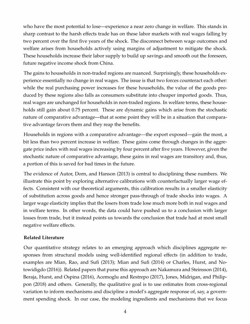
who have the most potential to lose—experience a near zero change in welfare. This stands insharp contrast to the harsh effects trade has on these labor markets with real wages falling bytwo percent over the first five years of the shock. The disconnect between wage outcomes andwelfare arises from households actively using margins of adjustment to mitigate the shock.These households increase their labor supply to build up savings and smooth out the foreseen,future negative income shock from China.

The gains to households in non-traded regions are nuanced. Surprisingly, these households ex-perience essentially no change in real wages. The issue is that two forces counteract each other:while the real purchasing power increases for these households, the value of the goods pro-duced by these regions also falls as consumers substitute into cheaper imported goods. Thus,real wages are unchanged for households in non-traded regions. In welfare terms, these house-holds still gain about 0.75 percent. These are dynamic gains which arise from the stochasticnature of comparative advantage—that at some point they will be in a situation that compara-tive advantage favors them and they reap the benefits.

Households in regions with a comparative advantage—the export exposed—gain the most, abit less than two percent increase in welfare. These gains come through changes in the aggre-gate price index with real wages increasing by four percent after five years. However, given thestochastic nature of comparative advantage, these gains in real wages are transitory and, thus,a portion of this is saved for bad times in the future.

The evidence of Autor, Dorn, and Hanson (2013) is central to disciplining these numbers. Weillustrate this point by exploring alternative calibrations with counterfactually larger wage ef-fects. Consistent with our theoretical arguments, this calibration results in a smaller elasticityof substitution across goods and hence stronger pass-through of trade shocks into wages. Alarger wage elasticity implies that the losers from trade lose much more both in real wages andin welfare terms. In other words, the data could have pushed us to a conclusion with largerlosses from trade, but it instead points us towards the conclusion that trade had at most smallnegative welfare effects.

Related Literature

Our quantitative strategy relates to an emerging approach which disciplines aggregate re-sponses from structural models using well-identified regional effects (in addition to trade,examples are Mian, Rao, and Sufi (2013); Mian and Sufi (2014) or Charles, Hurst, and No-towidigdo (2016)). Related papers that purse this approach are Nakamura and Steinsson (2014),Beraja, Hurst, and Ospina (2016), Acemoglu and Restrepo (2017), Jones, Midrigan, and Philip-pon (2018) and others. Generally, the qualitative goal is to use estimates from cross-regionalvariation to inform mechanisms and discipline a model’s aggregate response of, say, a govern-ment spending shock. In our case, the modeling ingredients and mechanisms that we focus

4

on are strongly informed by the evidence of Autor, Dorn, and Hanson (2013) and Greenland,Lopresti, and McHenry (2017). In a similar sprit, through a procedure which is essentiallysimulated method of moments, we ask our model match the cross-reginal empirical outcomes.Moreover, our model provides a clear interpretation about how these empirical moments mapinto model parameters.

Quantifying the aggregate effects of a trade shock are central to pinning down the level withregards to the distributional effects. A weakness of the research design in Autor, Dorn, andHanson (2013) and related evidence is that these estimates are only able to make statementsabout differential effects—not levels, see, e.g. the discussion in Nakamura and Steinsson (2018).In the case of trade, this critique is particularly pertinent as an optimistic interpretation of theevidence is that all labor markets gained from trade with China, just some gained more thanothers. Substantively, the disconnect between estimated differential effects and levels showsup prominently in the result that the China shock caused an increase employment by a millionand a half at the aggregate level.

Our work is also closely related to growing body work on trade and labor market dynam-ics (see, e.g., Kambourov (2009), Artuc, Chaudhuri, and McLaren (2010), Dix-Carneiro (2014),Caliendo, Dvorkin, and Parro (2015), Cosar, Guner, and Tybout (2016)). Our key departure fromthis literature is the focus on an the incomplete market setting. While there are important costsassociated with our approach—we are unable to incorporate the the geographic and sectoraldetail found in Caliendo, Dvorkin, and Parro (2015)— there are benefits of what we are doingfor several reasons.

The first reason relates to normative issues. Even if there were losses in income and employ-ment opportunities, open questions are: How large are the losses in welfare? We believe thatissue here is the extent of market incompleteness and the ability of households to adjust totrade shocks.1 The standard gains from trade argument is that there exists a transfer schemeto compensate the losers from trade—i.e., even with losses in the labor market, transfers alloweveryone to enjoy the aggregate gains from trade. In contrast, if households are an island tooneself with no transfers or insurance markets, the welfare losses could be large. Thus, an im-portant contribution of this paper is examine the distributional effects of trade in a standard,intermediate setting—the standard incomplete markets model.

The second reason incomplete market setting also opens the door to questions about govern-ment policy which far understudied within this trade and labor market dynamics literature. Asan economy is increasingly exposed to trade does policy have an ability to improve outcomes?Can tariffs improve welfare? Difference-in-difference approaches are valuable, but they are

1The quantitative nature of our analysis distinguishes this paper from earlier discussions about risk, incompletemarkets, and the gains from trade, e.g., see Newbery and Stiglitz (1984) and Eaton and Grossman (1985) and Dixit(1987, 1989a,b).

5

unable to answer these policy relevant, normative questions. In contrast, our approach can en-tertain these questions. As one example, our parallel work in Lyon and Waugh (2018) exploresthese issues and finds that a progressive tax system is an important tool to mitigate the negativeconsequences of trade.

1. Motivating Facts

Below we discuss macro- and micro-level facts behind the expansion of US-Chinese trade.None of these facts are new, but they are important to state as they help motivate our mod-eling and calibration strategy.2

1.1. Macro Facts

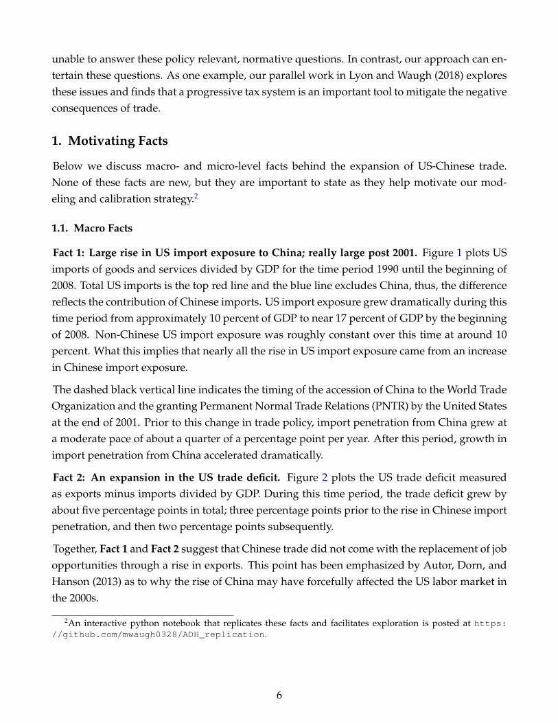
Fact 1: Large rise in US import exposure to China; really large post 2001. Figure 1 plots USimports of goods and services divided by GDP for the time period 1990 until the beginning of2008. Total US imports is the top red line and the blue line excludes China, thus, the differencereflects the contribution of Chinese imports. US import exposure grew dramatically during thistime period from approximately 10 percent of GDP to near 17 percent of GDP by the beginningof 2008. Non-Chinese US import exposure was roughly constant over this time at around 10percent. What this implies that nearly all the rise in US import exposure came from an increasein Chinese import exposure.

The dashed black vertical line indicates the timing of the accession of China to the World TradeOrganization and the granting Permanent Normal Trade Relations (PNTR) by the United Statesat the end of 2001. Prior to this change in trade policy, import penetration from China grew ata moderate pace of about a quarter of a percentage point per year. After this period, growth inimport penetration from China accelerated dramatically.

Fact 2: An expansion in the US trade deficit. Figure 2 plots the US trade deficit measuredas exports minus imports divided by GDP. During this time period, the trade deficit grew byabout five percentage points in total; three percentage points prior to the rise in Chinese importpenetration, and then two percentage points subsequently.

Together, Fact 1 and Fact 2 suggest that Chinese trade did not come with the replacement of jobopportunities through a rise in exports. This point has been emphasized by Autor, Dorn, andHanson (2013) as to why the rise of China may have forcefully affected the US labor market inthe 2000s.

2An interactive python notebook that replicates these facts and facilitates exploration is posted at https://github.com/mwaugh0328/ADH_replication.

6

1992 1994 1996 1998 2000 2002 2004 2006 20089

10

11

12

13

14

15

16

17

Impo

rts / G

DP

Non Chinese ImportsImportsChina WTO Accession

Figure 1: US Imports

1992 1994 1996 1998 2000 2002 2004 2006 20086

5

4

3

2

1

0

(Exp

orts

- Impo

rts) /

GDP

Trade Deficit / GDP

Figure 2: US Trade Deficit

7

1.2. Micro Facts

The next three facts focus on labor market outcomes from Autor, Dorn, and Hanson (2013)and migration responses in Greenland, Lopresti, and McHenry (2017). These studies exploitchanges in the variation in trade exposure at the commuting zone level (see Tolbert and Sizer(1996)) and correlate it with changes in labor market outcomes. The main measure of tradeexposure is:

∆IPWuit =∑j

(LijtLit

)(∆Mucjt

Lijt

)(1)

where u stands for united states, c stands for China, i is a commute zone, t is time, and j

is industry. This measure takes aggregate US imports from China Mucjt for industry j andapportions these imports to a commute zone based on that commute zones share of nationalemployment in that industry. It then aggregates across industries for that commute zone.

Given this measure of trade exposure, they estimate its affect on outcome Yit with the followingempirical specification:

∆Yit = γt + β∆IPWuit + controlsi + εit. (2)

One important issue with this specification is that the error term embeds factors that simulta-neously change a commute zone’s trade exposure and labor market outcomes. As our modelmakes clear (see Section 4), local productivity shocks is a key threat to identification as it wouldchange that commute zones comparative advantage and labor markets outcomes. To avoidthis problem, Autor, Dorn, and Hanson (2013)) estimate (2) using other countries imports fromChina as an instrument which would be correlated with US trade exposure, but orthogonal tolocal productivity shocks.

In the facts below, we report estimates after standardizing the ∆IPWuit. That is we demeanedthis measure and divided by its standard deviation. As in Autor, Dorn, and Hanson (2013) alllabor market outcomes are converted to 10 year changes.

Fact 3: Import exposure decreased household income. The first column in Table 1 reports Au-tor, Dorn, and Hanson’s (2013) estimate of the response of commute zone, average householdlabor income per adult to trade exposure. What this coefficient means is that a one standarddeviation increase in trade exposure reduced wage growth by four percent over 10 years. Toput this in context, average wage growth over the period 2000-2007 was only about six percent(converted to ten year change).

Fact 4: Import exposure increased non-participation. The second column in Table 1 reports

8

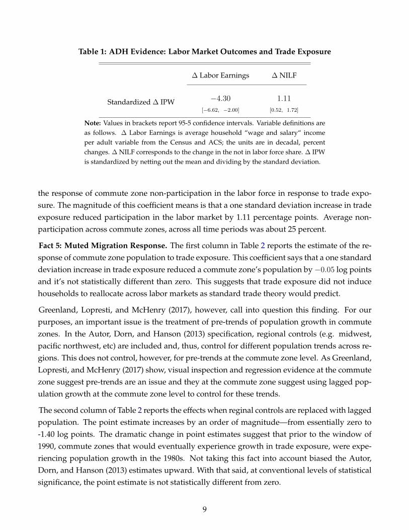
Table 1: ADH Evidence: Labor Market Outcomes and Trade Exposure

∆ Labor Earnings ∆ NILF

Standardized ∆ IPW −4.30

[−6.62, −2.00]

1.11

[0.52, 1.72]

Note: Values in brackets report 95-5 confidence intervals. Variable definitions areas follows. ∆ Labor Earnings is average household “wage and salary“ incomeper adult variable from the Census and ACS; the units are in decadal, percentchanges. ∆ NILF corresponds to the change in the not in labor force share. ∆ IPWis standardized by netting out the mean and dividing by the standard deviation.

the response of commute zone non-participation in the labor force in response to trade expo-sure. The magnitude of this coefficient means is that a one standard deviation increase in tradeexposure reduced participation in the labor market by 1.11 percentage points. Average non-participation across commute zones, across all time periods was about 25 percent.

Fact 5: Muted Migration Response. The first column in Table 2 reports the estimate of the re-sponse of commute zone population to trade exposure. This coefficient says that a one standarddeviation increase in trade exposure reduced a commute zone’s population by−0.05 log pointsand it’s not statistically different than zero. This suggests that trade exposure did not inducehouseholds to reallocate across labor markets as standard trade theory would predict.

Greenland, Lopresti, and McHenry (2017), however, call into question this finding. For ourpurposes, an important issue is the treatment of pre-trends of population growth in commutezones. In the Autor, Dorn, and Hanson (2013) specification, regional controls (e.g. midwest,pacific northwest, etc) are included and, thus, control for different population trends across re-gions. This does not control, however, for pre-trends at the commute zone level. As Greenland,Lopresti, and McHenry (2017) show, visual inspection and regression evidence at the commutezone suggest pre-trends are an issue and they at the commute zone suggest using lagged pop-ulation growth at the commute zone level to control for these trends.

The second column of Table 2 reports the effects when reginal controls are replaced with laggedpopulation. The point estimate increases by an order of magnitude—from essentially zero to-1.40 log points. The dramatic change in point estimates suggest that prior to the window of1990, commute zones that would eventually experience growth in trade exposure, were expe-riencing population growth in the 1980s. Not taking this fact into account biased the Autor,Dorn, and Hanson (2013) estimates upward. With that said, at conventional levels of statisticalsignificance, the point estimate is not statistically different from zero.

9

Table 2: ADH and GLM Evidence: Migration and Trade Exposure

ADH ∆ Population GLM, ∆ Population

Standardized ∆ IPW −0.05

[−1.51, 1.41]

−1.43

[−3.33, 0.48]

Note: Values in brackets report 95-5 confidence intervals. Variable definitions areas follows. ∆ Population corresponds with the log change in population. ∆ IPWis standardized by netting out the mean and dividing by the standard deviation.Greenland, Lopresti, and McHenry (2017) (GLM) replace ADH regional controlswith agged population growth at the commute zone level.

Greenland, Lopresti, and McHenry (2017) raise two other issues support the view that therewas a migration response. The first issue is the use of Census data versus nationally represen-tative samples; using Census data delivers similar point estimates in Table 2 but stronger andsignificant effects for the young vs. old. A second issue is the time window. Extending the win-dow to 2010 leads to statistically significant effects with point estimates comparable to Table 2.In sum, relative to the body of evidence provide by Greenland, Lopresti, and McHenry (2017)suggests that there was a migration response.

1.3. Discussion

Taken together, these facts suggest a compelling narrative: At the macro level, there was a largeincrease in import exposure from China and no corresponding increase in export opportunities.And at the micro level, the evidence suggest this wreaked havoc on labor market in the UnitedStates—households absorbed loses in labor income, stopped participating in the labor market,and with some migration from trade exposed regions.

How to interpret this evidence? First, there is an issue about the interpretation of the cross-sectional estimates in (1) and how to map them into aggregate conclusions. The model that wedevelop below plays an important role here. And as we describe in Section 4 the model bridgesthis gap, clarifies what these estimates are informative about, and we use these estimates asinputs into our quantitative analysis.

Second, a model is needed to jump from changes in income and non-participation to state-ments about welfare. Our presumption is that while households have limited access to directinsurance markets, they do have a myriad of ways to smooth out negative labor market out-comes: one is self-insurance, another is that changes in participation can mitigate and assistself-insurance, a third is migration. Thus, our model that allows us to entertain multiple, stan-

10

dard mechanisms for which households can mitigate the negative shocks.

A final issue relates to the trade deficit. Traditional trade theory’s perspective on this suggeststhat increases in import penetration from China did not come with increases in export andemployment opportunities for those displaced from trade. This perspective ignores the ideathat a rising trade deficit implies households are increasing their consumption above and be-yond their savings. In other words, the of China came with an expansion of both intra- andinter-temporal trading opportunities.

2. Model

This section describe a model of international trade with households facing incomplete mar-kets and frictions to move across labor markets. The first subsection discusses the productionstructure; the second subsection discusses discusses the households.

Below, since we focus on the perspective of one country, country subscripts are omitted unlessnecessary. Similarly, time subscripts are omitted unless necessary.

2.1. Production

The model has an intermediate-goods sector and a final good sector that aggregates the in-termediate goods. Within a country, there is a continuum of intermediate goods indexed byω ∈ [0, 1]. As in the Ricardian model of Dornbusch, Fischer, and Samuelson (1977) and Eatonand Kortum (2002), intermediate goods are not nationally differentiated. Thus, intermediateω produced in one country is a perfect substitute for the same intermediate ω produced byanother country.

Competitive firms produce intermediate goods with linear production technologies,

q(ω) = z(ω)`, (3)

where z is the productivity level of firms and ` is the number of efficiency units of labor. Inter-mediate goods productivity evolves stochastically according to an AR(1) process in logs

log zt+1 = φ log zt + εt+1, (4)

where εt+1 is distributed normally with mean zero and standard deviation σε. The innovationεt+1 is independent across time, goods, and countries.

Firms producing variety ω face competitive product and labor markets with households thatsupply labor elastically. Competition implies that a household choosing to work in market ωearns the value of its marginal product of labor, which is the price of the good times the firm’s

11

productivity z.

Transporting intermediate goods across countries is costly. Specifically, consumers and firmsface iceberg trade costs when importing and exporting their products. We allow for the importand export cost to differ with τim > 1 being the cost to import a good from abroad and τex > 1

being the cost an export faces to ship goods onto the world market.

Intermediate goods are aggregated by a competitive final-goods produce who has a standardCES production function:

Q =

[∫ 1

0

q(ω)ρdω

] 1ρ

, (5)

where q(ω) is the quantity of individual intermediate goods ω demanded by the final-goodsfirm, and ρ controls the elasticity of substitution across variety, which is θ = 1

1−ρ .

2.2. Households

Within a country, there is a continuum of infinitesimally small households of mass L. Eachhousehold is infinitely lived and maximizes expected discounted utility

E∞∑t=0

βt{

log(ct)−Bh1−γt

1− γ+ νit

}, (6)

where E is the expectation operator and β is the subjective discount factor. Period utility de-pends on both consumption of the final good, the disutility of labor, and a preference shock νit .The preference shock νit is index by i which corresponds with choice of the household to moveor not. As in Artuc, Chaudhuri, and McLaren (2010) and Caliendo, Dvorkin, and Parro (2015),this preference shock is independently and identically distributed across time and is distributedType 1 extreme value distribution with scale parameter σν .

Households live and work along the same dimension as the intermediate goods. That is, ahousehold’s location is given by ω—the intermediate goods sector in which it can work. Giventheir current location, households can choose to work, to move and work someplace else in thefuture, and to accumulate a non-state contingent asset. Below, we describe each of these choicesin detail.

Working is a discrete choice between zero hours and h. Thus, the labor supply is purelyon the extensive margin. If a household works, it receives income from employment in theintermediate-goods sector in which the household resides. In the following presentation, wenormalize the value h equal to one. If a household does not work, if receives home productionwh. The value of home production partially determines the value of being out of the labor force

12

and hence, the elasticity of labor supply on the extensive margin.

Households can move to an alternative intermediate-goods sector ω′ at some cost. Paying m inunits of the final good allows the household to change where it can work in next period. Weassume that the new location is a random labor market. Moving also triggers the realization ofthe ν preference shock associated with the move.

Households residing in a intermediate-goods location face labor income risk associated withfluctuations in local productivity and fluctuations in world prices. We do not allow for anyinsurance markets against this risk, but let households accumulate a non-state contingent asseta that pays gross return R. We treat R as exogenous and not solved for in equilibrium. Aninterpretation is that this country faces a large supply of assets at this rate. Households face alower bound on asset holding −a, so agents can acquire debt up to the value a.

State Variables. The individual state variable of a household are its location, asset holdingsa, and preference shocks νi. The island-level state variable is the domestic productivity stateand world price state. The aggregate state is a distribution over island-level state variables andasset holdings.

Let us expand on this a bit more. The wage per efficiency unit that a household receives isa important island-level object impacting individual decisions. The wage per efficiency unitdepends on the value of the marginal product of labor on that island. The marginal productdepends on a country’s productivity level. The “value” part depends on (i) the world price and(ii) the labor supply decisions of households residing on the island. Given our preference spec-ification in (6), households’ labor supply decisions depend on the distribution of asset holdingswithin the island. Thus, this is where the aggregate state matters for island-level outcomes.

The presentation below depicts a stationary equilibrium. That is, the aggregate state—the dis-tribution over island level states and assets holdings—is constant.3 Thus, to conserve on no-tation, we only carry around the households specific state variables: its own asset holdings,preference shocks, and island-level state variables associated with its location. In particular, lets denote the domestic productivity and world price combination associated with that island.Furthermore, because the CES aggregator is symmetric over varieties, it is sufficient to indexislands by their productivity and world price state. The wage per efficiency unit a householdearns is w(s).

Budget Constraints. Given the description of the environment, the budget constraints are asfollows. For households that are working, the household’s period t budget constraint (all de-

3Given an island with state s, denote the measure of agents with asset holdings a as λ(s, a). Stationarity impliesthat this value is constant.

13

nominated in units of the final good) is

at+1 + ct + ιm,tm ≤ Rat + wt(s), (7)

where the left-hand side are expenditures on new assets, consumption, and possibly movingcosts with ιm,t being an indicator function equaling one if a household moves and zero other-wise. The right-hand side are income payments from asset returns and labor income.

If a household is not working, then the budget constraint is modified to ensure that homeproduction is not used to accumulate assets or pay for moving costs. In this case, a non-workinghouseholds budget constraint is

ct ≤ wh + |Rat − at+1 − ιm,tm|+, (8)

where the right-hand side is home production plus any positive income from net asset holdings,net of moving costs. What this formulation insures is the home prosecution is just that. It cannot be used for purchases in the market of assets of moving costs.

Recursive Formulation. The recursive formulation of the household’s problem is

V (a, s, ν) = max [V s,w, V s,nw, V m,w, V m,nw] . (9)

that is a discrete choice among four options: the value of staying and working; the value ofstaying and not working; the value of moving and working; the value of moving and not work-ing. Unpacking each of these four options is the following. The value of staying and workingis

V s,w(a, s, ν) = maxa′≥−a

[u(Ra+ w(s)− a′)−B + νs + βEV (a′, s’, ν ′)] , (10)

where u is the utility value over consumption and νs is the preference shock associated withstaying in its current location. The value of staying and not working is

V s,nw(a, s, ν) = maxa′≥−a

[u(wh + |Ra− a′|+) + νs + βEV (a′, s’, ν ′)

]. (11)

The value of moving and working is

V m,w(a, s, ν) = maxa′≥−a

[u(Ra+ w(s)− a′ −m)−B + νm + βV m(a′)] , (12)

where there are several key distinctions relative to (10). First, the moving cost, m is paid. Sec-ond, νm is the preference shock associated with moving. Third, the continuation value is V m(a′)

14

or the value associated with a move. Finally, the value of moving and not working is

V m,nw(a, s, ν) = maxa′≥−a

[u(wh + |Ra− a′ −m|+) + νm + βV m(a′)

]. (13)

3. Equilibrium

We close the model by focusing on a small open economy equilibrium. The small open econ-omy assumption is that there is no feedback from home country actions into world prices.4

World Prices. World prices for commodity ω evolve according to an AR(1) process in logs:

log pw(ω)t+1 = φ log pw(ω)t + ε(ω)t+1, (14)

where ε(ω)t is distributed normally with mean zero and standard deviation σw and is indepen-dent of the innovation to the home country’s productivity εt. We express these prices in unitsof the numeraire, which we take to be the final good in the home country.

A Note on Notation. We denote π(s) as the stationary distribution of productivity states andworld prices induced by (4) and (14). And denote µ(s) as the measure of households workingon an island with state s. This value is defined later in (27) and integrates over the labor supplychoice of households (which depends upon their individual states and preference shocks).

3.1. Production Side of the Economy

Below, we describe the equilibrium conditions associated with the production side of the econ-omy. These take as given the choices of the household.

Final Goods Production. The final-goods producer’s problem is:

maxq(s)

PhQ−∫p(s)q(s)π(s)ds, (15)

which gives rise to the following the demand curve for an individual variety:

q(s) =

(p(s)

Ph

)−θQ. (16)

where Q is the aggregate demand for the final good; Ph is the price associated with the finalgood which will be carried around briefly, but is ultimately normalized to the value one.

4Relative to the trade and labor market dynamics literature, this is similar to the second specification solved inArtuc, Chaudhuri, and McLaren (2010). Moreover, it has the advantage (say, relative to Caliendo, Dvorkin, andParro (2015)) of being relatively simple, yet allows us to specific about the interaction between trade flows andcapital flows.

15

Intermediate Goods Production. The intermediate-goods-producer’s problem is

maxq(s),`(s)

p(s)q(s)− w(s)`(s) (17)

or to choose the quantity produced to maximize profits. Competition implies that the wage perefficiency unit (in units of the final good) at which a firm hires labor is:

w(s) = p(s)z (18)

or the value of the marginal product of labor. Only at the wage in (18) are intermediate-goodsproducers willing to produce.

Intermediate Goods, International Trade, and Market Clearing. To formulate the pattern oftrade, we denote the set of prevailing prices that the final-goods producer in the home countryfaces as p(s) , τimpw , pw/τex. The final-goods producer purchases intermediate goods from thelow-cost supplier. This decision gives rise to three cases with three different market-clearingconditions: if the good is non-traded; if the good is imported; and if the good is exported.5

Below, we describe demand and production in each of these cases.

• Non-traded. If the good is non-traded, then the domestic price for the home country mustsatisfy the following inequality: pw

τex< p(s) < τimpw. That is, from the home country’s

perspective, it is optimal to source the good domestically and not optimal for the homecountry to export the product.

In this case, the market-clearing condition is:(p(s)

Ph

)−θQ = z (µ(s)/π(s)) (19)

or that domestic demand equals production. The left-hand part is demand and the right-hand side is supply. That is the the productivity of domestic suppliers multiplied by thesupply of labor units in that market.

• Imported. If the good is imported, then the domestic price for the home country mustbe p(s) = τimpw. Why? If the price were lower, then it would not be imported. If thedomestic price were higher, then the good will be imported with not domestic productionand, thus, the prevailing domestic price will equal the imported price. With frictional

5This is more nuanced than the standard formulation in Eaton and Kortum (2002) due to the frictional labormarket. In our model, there are situations in which an intermediate good is both imported and produced domes-tically, which is not the case in the Eaton and Kortum (2002) model.

16

labor markets, there may be some domestic production so the quantity of imports is((τimpwPh

)−θQ

)− z (µ(s)/π(s))︸ ︷︷ ︸

imports

> 0. (20)

That is home demand (net of home production) is met by imports of the commodity.Rearranging gives ((

τimpwPh

)−θQ

)= z (µ(s)/π(s)) + imports(s) (21)

or domestic demand equals domestic production plus imports.

• Exported. If the good is exported, then the prevailing price must be p(s)τex = pw. Why? Ifthe home price were larger, then the good would not be purchased on the world market.And the price can not be lower, as arbitrage implies that the price of the exported goodsold in the world market must equal the prevailing price in that market. Finally, note thatonly the trade cost, not the tariff, matters here. At this price, the quantity of exports is(

pw/τexPh

)−θQ− z (µ(s)/π(s))︸ ︷︷ ︸

− exports

< 0 (22)

or domestic demand net of production which should be negative, implying that the coun-try is an exporter. Rearranging gives(

pw/τexPh

)−θQ = z (µ(s)/π(s)) − exports(s) (23)

or domestic demand equals domestic production minus exports.

The Final Good and Market Clearing. The final good’s producer sells the final good to con-sumers. Thus, we have the following market-clearing condition

Q = C =

∫s

∫a

∫ν

c(s, a, ν)λ(s, a, ν)dν da ds, (24)

where c(s, a, ν) is the consumption policy function that satisfies the households’ problem, andλ(s, a, , ν) is the mass of consumers with state s, asset holding a, and preference shock ν (definedbelow in (??)). This relationship says that household-level consumption—aggregated across allhouseholds— must equal the aggregate production of the final good Q.

17

Market-clearing conditions for the intermediate goods in (19),(21), (23) and the aggregate finalgood in (24) summarize the equilibrium relationship on the production side of the economy.

3.2. Household Side of the Economy

The households in the economy make choices about where to reside, how much to work, andhow much to consume. Here, we describe the equilibrium conditions associated with thesechoices. In the discussion below, we define the following functions—{ ιm(s, a, ν), ιn(s, a, ν), ga(s, a, ν) }—as the move, work, and asset policy functions that satisfy the households’ problem in (9).

The distribution of households across states. We define the probability distribution of house-holds across assets and states as λ(s, a, ν). Furthermore, define the probability distribution ofhouseholds in the next period as λ′(s′, a′, ν ′). The distribution of households evolves across timeaccording to the following law of motion:

λ′(s’, a′, ν ′) = φ(ν ′)

∫s

∫ν

∫a:a′=ga(s,a,ν)

λ(s, a, ν)(1− ιm(s, a, ν))π(s’, s) + λ(s, a, ν)ιm(s, a, ν)π(s’) da dν ds.

(25)

Equation (25) says that in the next period, the mass of households with asset holding a′ in states’ with preference shock ν ′ equals several terms. First, the probability that preference shocksν ′ are realized where φ is the probability density function associated with the Type 1 extremevalue distribution. The second term is the mass of household that do not move multiplied bythe transition probability that s transits to s’—this is the first term in equation (25). The thirdterm is the mass of households that do move, multiplied by the probability that they end up instate s’—this is the second term in equation (25). The probability, π(s’), is given by the movingprotocol—i.e., random assignment across islands according to the invariant distribution associ-ated with π(s’, s). All of this is conditional on those households that choose asset holdings equalto a′, this is denoted by the conditionality under the innermost integral sign. And integratedacross preference shocks and current island state s.

Population and Labor Supply. Given a distribution of households, we define the populationof households on islands with state s as∫

ν

∫a

λ(s, a, ν)da dν. (26)

In words, the population is found by just integrating over the mass across asset holdings andpreference shocks.6 Then the supply of labor to intermediate good producers with productivity

6This calculation should be distinguished by the population on an individual island. This is latter value isfound by dividing 26 by the measure of that island type.

18

state s is,

µ(s) =

∫ν

∫a

ιn(s, a, ν)λ(s, a, ν)da dν, (27)

which is the size of the population residing in that market multiplied by the labor supply policyfunction and integrated over all asset states. This, then, connects the supply of labor withproduction in (19)-(23).

Asset Holdings. The distribution of asset holdings and consumption take the following form.Next period, aggregate net-asset holdings are

A′ =∫ν

∫a

∫s

ga(s, a, ν)λ(s, a, ν)ds da dν, (28)

where ga(s, a, ν) is the policy function describing asset holdings tomorrow, given the states to-day. A couple of points about this are warranted. First, this is in aggregate—some householdsmay have positive holdings, while others may have negative holdings. Second, net asset hold-ings must always be claims on foreign assets since there is no domestic asset in positive supply(such as capital).

3.3. A Stationary Small Open Economy (SSOE) Equilibrium

Given the equilibrium conditions from the production and household side of the economy, wedefine a “Stationary Small Open Economy (SSOE) Equilibrium” equilibrium.

A Stationary Small Open Economy (SSOE) Equilibrium. Given world prices {pw, R}, a sta-tionary Small Open Economy Equilibrium is domestic prices {p(s)}, policy functions{ ga(s, a, ν), ιn(s, a, ν), ιm(s, a, ν) }, and a probability distribution λ(s, a, ν) such that

i Firms maximize profits, (15) and (17) ;

ii The policy functions solve the household’s optimization problem in (9);

iii Demand for the final and intermediate goods equals production, (19), (20), (22) and (24);

iv The probability distribution λ(s, a, ν) is a stationary distribution associated with{ ga(s, a, ν), ιm(s, a, ν), π(s’, s, ν) }. That is, it satisfies

λ(s’, a′, ν ′) = φ(ν ′)

∫s

∫ν

∫a:a′=ga(s,a,ν)

λ(s, a, ν)(1− ιm(s, a, ν))π(s’, s) + λ(s, a, ν)ιm(s, a, ν)π(s’) da dν ds.

(29)

19

The idea behind the equilibrium definition is the following. The first bullet point (i) gives riseto the equilibrium conditions for the demand of intermediate goods in (16) and wages (18)at which firms are willing to produce. The second bullet point (ii) says that households areoptimizing.

At a superficial level, bullet (iii) says that demand must equal supply. It’s meaning, however,deeper. The households’ choices of the matter for both the demand and the supply side. Specif-ically, it requires that prices (and, hence, wages) must induce a pattern of (i) consumption and(ii) labor supply such that demand for goods equals the production of goods.

Bullet point (iv) requires stationarity. Specifically, the distribution of households across produc-tivity and asset states is not changing. Mathematically, this means that distribution λ(s, a, ν)

must be such that when plugged into the law of motion in (25), the same distribution is re-turned.

Finally, note that there is no requirement that the asset market clears—i.e., that (28) equalszero. This is an aspect of the small open economy assumption. At the given world interest rateR, the assets need not be in zero net supply. This implies that trade need not balance, as thetrade imbalance will reflect asset income on foreign assets and the acquisition of assets. Afteradjusting for moving costs, this implies that the current account and capital account are alwayszero in a stationary equilibrium, but that trade may be imbalanced.

Computation. Computing a stationary equilibrium for this economy deserves some discussion.First, this economy is unlike standard incomplete markets models in which only one or twoprices (e.g., one wage per efficiency unit and/ or the real interest rate) must be solved for. Incontrast, we must solve for an equilibrium function p(s). Thus, the iterative procedure is to (i)guess a price function; (ii) solve the household’s dynamic optimization problem; (iii) constructthe stationary distribution λ(s, a, ν); (iv) check whether markets clear; and (v) update the pricefunction. See, e.g., Krusell, Mukoyama, and Sahin (2010), who solve a similar problem.

Second, while the household’s problem contains three state variables, the i.i.d. assumption onν allows us to integrate out the preference shock, compute choice probabilities, and then workdirectly on the distribution across islands and asset states, i.e. λ(s, a).7 The Type 1 extreme valuedistribution allows us to perform this integration step in closed form. In addition to allowingour model to match certain targets, these preference shocks also make the aggregate economycontinuous in its price (modulo the discussion below) and parameter space which facilitatesthe quick computation of solutions to a stationary equilibrium.

Third, an important observation is that the inequalities in (20) and (22) impose additional struc-

7To see this point, simply examine (25) and first integrate out the ν’s. Integrating the individual policy functionsover the νs are the choice probabilities of a particular action, given state s, a, which take the familiar logit formgiven the distributional assumption.

20

ture on an equilibrium. The observation is that when domestic demand and supply are notequal, the price in those markets must respect bounds on international arbitrage. This im-plies that the problem of finding a price function consistent with a stationary equilibrium canbe represented as a mixed complementarity problem (see, e.g., Miranda and Fackler (2004)).Appendix B provides a complete description of our solution procedure and links to our coderepository.

4. Model Properties

This section describes some qualitative properties of the model. Below we focus on three issues(i) the pattern of trade across labor markets (ii) how trade exposure affects wages and howour model relates to the empirical approach/specification of Autor, Dorn, and Hanson (2013).Finally, we use these results to motivate our quantitative exercise.

4.1. Trade

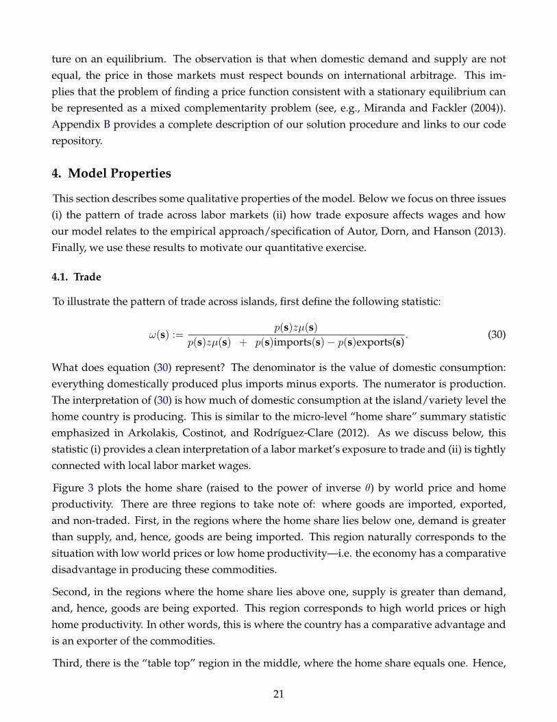
To illustrate the pattern of trade across islands, first define the following statistic:

ω(s) :=p(s)zµ(s)

p(s)zµ(s) + p(s)imports(s)− p(s)exports(s). (30)

What does equation (30) represent? The denominator is the value of domestic consumption:everything domestically produced plus imports minus exports. The numerator is production.The interpretation of (30) is how much of domestic consumption at the island/variety level thehome country is producing. This is similar to the micro-level “home share” summary statisticemphasized in Arkolakis, Costinot, and Rodrıguez-Clare (2012). As we discuss below, thisstatistic (i) provides a clean interpretation of a labor market’s exposure to trade and (ii) is tightlyconnected with local labor market wages.

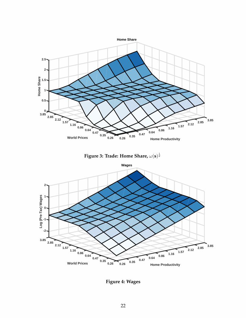
Figure 3 plots the home share (raised to the power of inverse θ) by world price and homeproductivity. There are three regions to take note of: where goods are imported, exported,and non-traded. First, in the regions where the home share lies below one, demand is greaterthan supply, and, hence, goods are being imported. This region naturally corresponds to thesituation with low world prices or low home productivity—i.e. the economy has a comparativedisadvantage in producing these commodities.

Second, in the regions where the home share lies above one, supply is greater than demand,and, hence, goods are being exported. This region corresponds to high world prices or highhome productivity. In other words, this is where the country has a comparative advantage andis an exporter of the commodities.

Third, there is the “table top” region in the middle, where the home share equals one. Hence,

21

03.85

0.5

2.85

1

2.12 3.851.57 2.85

Ho

me

Sh

are

1.5

2.121.16

Home Share

World Prices

1.57

2

0.86

Home Productivity

1.16

2.5

0.64 0.860.640.47 0.470.35 0.350.26 0.26

Figure 3: Trade: Home Share, ω(s)1θ

3.85

-2

2.85

-1

2.12 3.851.57

0

2.85

Lo

g (

Pre

-Tax

) W

ages

2.121.16

Wages

World Prices

1

1.570.86

Home Productivity

1.16

2

0.64 0.860.640.47 0.470.35 0.350.26 0.26

Figure 4: Wages

22

this is the region where the goods are non-traded. Exactly like the inner, non-traded region inthe Ricardian model of Dornbusch, Fischer, and Samuelson (1977), the reason is trade costs. Inthis region, world prices and domestic productivity are not high enough for a producer to bean exporter of these commodities given trade costs. Furthermore, world prices and domesticproductivity are not low enough to merit importing these commodities either. Thus, thesegoods are non-traded.

Finally, unlike Dornbusch, Fischer, and Samuelson (1977) or Eaton and Kortum (2002), it is im-portant to reflect on the stochastic nature of this economy. While the stationary equilibrium ofthe economy leads to the stationary pattern of trade seen in Figure 3, individual islands transitbetween different states (world prices and domestic productivity). For example, an island maybe an exporter, but given a sequence of bad productivity shocks, the island will stop exportingand maybe even become an importer of a commodity it once exported.

4.2. Trade and Wages

One can connect the pattern of trade across islands/labor markets in Figure (3) with the struc-ture of wages in the economy. As we show in the Appendix, real wages in a market with statevariable s equal

w(s) = ω(s)1θ µ(s)

−1θ z

θ−1θ C

1θ . (31)

Here ω(s) is the home share defined in (30); µ(s) = µ(s)π(s)

is the number of labor units; z is domesticproductivity; C is aggregate consumption.

Equation (31) connects the trade exposure measure in (30) with island-level wages. A smallerhome share implies that wages are lower with elasticity 1

θ. This means that if imports (relative

to domestic production) are larger, then wages in that labor market are lower. Similarly, a largerhome share means that wages are higher.

While this looks like the “micro-level” analog of the aggregate result of Arkolakis, Costinot, andRodrıguez-Clare (2012) it is different in one important respect: the micro-level wage responseto micro-level trade exposure to trade takes the exact opposite sign.

Figure 4 illustrates these observations by plotting the logarithm of pre-tax wages by world priceand home productivity so it exactly matches up with Figure 3 . As equation (31) makes clear,there is a tight correspondence between wages and the home share in Figure 3. As in Figure 3,there are three regions to take note of.

The first region is where import competition is prevalent (low world prices or low home pro-ductivity) wages are low. A way to understand this result is as follows: wages reflect the valueof the marginal product of labor. In import competing islands, trade results in lower prices and,

23

hence, lower wages. The second region is where exporting is prevalent. Exporting regions areable to capture high world prices, and, thus, wages are high in these islands. Finally, the centerregion is where commodities are non-traded. Here, the gradient of wages very much mimicsthe increase in domestic productivity. In contrast, where goods are imported or exported, thewage gradient mimics the the change in world prices.

Again, it is important to reflect on the stochastic nature of this economy. While the stationaryequilibrium of the economy results in a stationary distribution of wages, individual islands(and households living on those islands) transit between different states (world prices and do-mestic productivity). For example, an island may be an exporter with households receivinghigh wages, but given a sequence of bad productivity shocks, the island will stop exporting,and household wages will fall.

Finally, equation (31) connects with the aggregate gains from trade. Any change in aggregatetrade exposure will also change in aggregate consumption, i.e. the C term. That is all workersbenefit from the“aggregate gains to trade”, but the island-level incidence will vary with itstrade exposure and may mitigate or completely offset the aggregate benefits from trade.

4.3. Connection with Autor, Dorn, and Hanson (2013)

The preceding results relate closely to the empirical specification and evidence of Autor, Dorn,and Hanson (2013) and Acemoglu, Autor, Dorn, Hanson, and Price (2016) that link changes intrade exposure with labor market outcomes such as wages (see Section IV.B of Autor, Dorn, andHanson (2013) ). To do illustrate the connection, start with (31) and take log differences acrosstime yielding

∆ logw(s) =1

θ∆ log (ω(s)/µh(s)) +

1

θ∆ logC︸ ︷︷ ︸γt

+ ∆ log(zθ−1θ

)︸ ︷︷ ︸

εs,t

, (32)

which says that the change in wages across locations is summarized by (i) trade exposure viathe change in per-worker home share, (ii) the change in aggregate consumption and (iii) thechange in location-specific productivity.

Equation (32) is closely related to the empirical specification of Autor, Dorn, and Hanson (2013)(see equation (5)). Autor, Dorn, and Hanson (2013) relate various labor market outcomes at thecommute zone level to commute-zone-level measures of trade exposure. Put in their terms,our theory connects changes in wages on the left hand side with trade exposure, an aggregateeffect (which would be picked up by the constant/or time effect), and the error term reflectsunobserved commute-zone-level productivity shocks.

Consistent with their arguments, equation (32) makes clear that an instrumental variable strat-

24

egy is necessary to identify the causal effect of trade exposure on wages. Commute-zone-levelproductivity shocks are unobserved, but correlated with trade exposure and, thus, trade expo-sure could increase either because of changes in world prices or domestic productivity.

The structure of the model suggests several instrumental variable strategies. One valid instru-ment would be to use the world price (if observed) directly. The world price is orthogonal todomestic productivity (the exclusion restriction), yet correlated with the home trade share. Theexclusion restriction follows from our small open economy assumption and the specificationthat the stochastic process in (14) that is assumed to be orthogonal to z.8 An alternative strategywould be to use another country’s imports as an instrument. Another country’s imports wouldbe orthogonal to the home country’s productivity, but correlated with world prices. This, infact, is quite similar to the instrument proposed in Autor, Dorn, and Hanson (2013).

4.4. Labor Supply

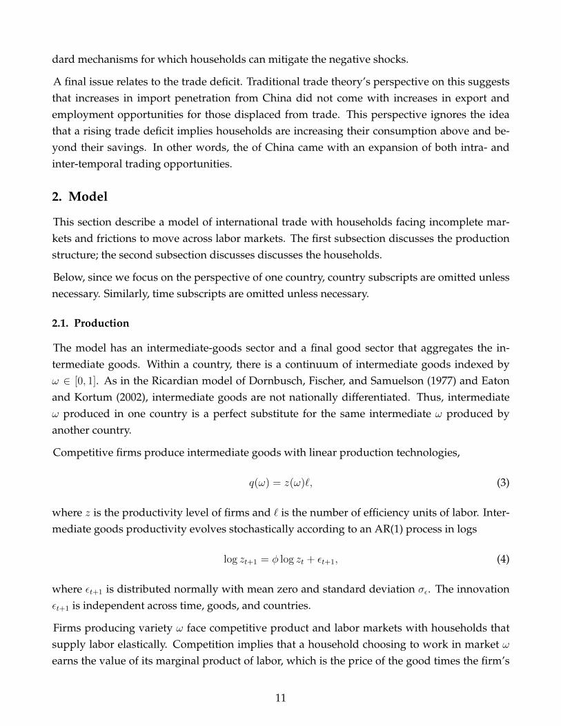
Figures 9 plots the policy functions for labor supply in the calibrated economy. Because thereare multiple dimensions of heterogeneity, this plots the policy functions for a given z and thenillustrates how labor supply varies across asset holdings and trade exposure. The distributionof asset holdings (for that z) is plotted to the right. Darker colors mean that more are likely tonot work, lighter colors mean that working is stronger.

Either by looking across panels or within a panel across trade exposure, households are gen-erally more likely to work the better labor market conditions. For example, the colors in themedium z panel are generally lighter than those in the low z case. Or when making compari-son within a z panel as trade exposure lessens (and wages improve) the colors become lighter,households are generally participating more.

With that said, there are economically interesting non-linearities that arise because of wealtheffects and the ability to use migration as an insurance mechanism. For example, focus on themost trade exposed area of the low z panel. In this labor market, the wealthiest households arenot participating. Like in Chang and Kim (2007), wealthy households have a high reservationwage because they can simply enjoy leisure and consume of their large stock of assets. Andbecause the low z, high trade exposed region will have a low wage, these households do notparticipate.

However, participation is not monotone in wealth. For the low z island, at the top of the bot-tom half of the asset distribution, participation is near one hundred percent. What makes thisregion special is households there are close to the minimum amount that they need to migrate.Thus, these households participate in the labor market to work, save, and preserve the option

8Moveover, the model makes clear that one should be concerned, in general equilibrium, that a change indomestic productivity would feed into world prices and, thus, invalidate this strategy.

25

Larg

er A

sset

Hol

ding

s

Less Import Exposure

0.0

0.2

0.4

0.6

0.8

1.0

Pro

babi

lity

of N

ot W

orki

ng

Asset Distribution

Low Z Labor Supply Policy Function

Larg

er A

sset

Hol

ding

s

Less Import Exposure

0.0

0.2

0.4

0.6

0.8

1.0

Pro

babi

lity

of N

ot W

orki

ng

Asset Distribution

Med. Z Labor Supply Policy Function

Figure 5: Labor Supply by Assets and Trade Exposure

26

of moving to a better market. Households are working to self insure, but not through assetaccumulation, but through migration.

Below the bottom half of the asset distribution households stop participating. These house-holds don’t have and can not acquire the resources to migrate, the labor market is poor, thustheir best option is simply to drop out of the labor force and receive leisure and home produc-tion. Home production is critical here as without it, households would prefer to work and, inturn, be able to consume.

4.5. Migration

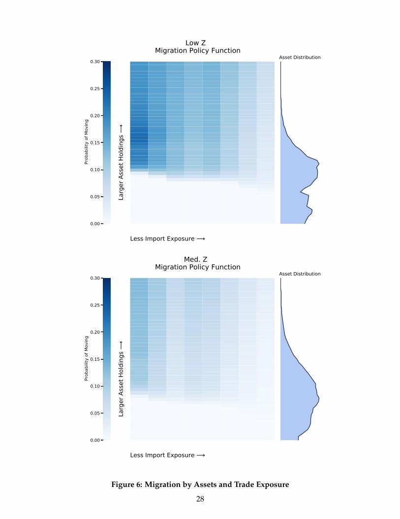
Figure 6 illustrates how migration varies across states. Similar to the labor supply figures, thisplots the policy functions for a given z and then illustrates how the moving choice varies acrossasset holdings and trade exposure. Again, the distribution of asset holdings is plotted to theright.

Current income, through the z and pw shocks, play a very strong role in shaping migration. Inlow z islands, and in particular high trade exposed islands, the desire to move is very strong.In contrast, on medium z islands, the desire to migrate is far more modest. The key idea here isthat the migration motive in our model is for insurance. That is, households undertake costlymoves to escape negative labor market conditions in one location and capture favorable labormarket conditions in another location.

Asset holdings, however, constrain who can move and who cannot. In the bottom of bothpanels, this can bee seen in the white sections with no migration for all levels of trade exposure.Households in this region do not have the financial means to migrate.

Asset holdings and income shocks interact though a “double whammy” effect—those with thestrongest desire to move are likely not to have the means to do so. In the low z and high tradeexposed islands, the desire to out migrate is the strongest. However, because those on lowz islands likely have experienced a sequence of negative shocks their asset holdings are likelyinsufficient to afford a move. This can be seen by noting the large mass of households with assetholdings in the region where moves are not feasible. Thus, the double whammy of wanting tomove, but can’t move. In contrast, consider the medium z panel. Here the desire to move ismodest even for those islands who are the most trade exposed. But the households on theseislands are also much wealthier and have greater means to afford a move. In other words, theseguys don’t want to move, but they could if they wanted.

These observations lead to a couple of issues that are worth pointing out. First, market incom-pleteness is interacting with the migration decision. From a positive stand point, this interac-tion is one reason why our model is able to match the low migration response in Table 2. Froma normative stand point, this interaction suggests that the welfare costs of trade exposure for

27

Larg

er A

sset

Hol

ding

s

Less Import Exposure

0.00

0.05

0.10

0.15

0.20

0.25

0.30

Pro

babi

lity

of M

ovin

g

Asset Distribution

Low Z Migration Policy Function

Larg

er A

sset

Hol

ding

s

Less Import Exposure

0.00

0.05

0.10

0.15

0.20

0.25

0.30

Pro

babi

lity

of M

ovin

g

Asset Distribution

Med. Z Migration Policy Function

Figure 6: Migration by Assets and Trade Exposure

28

certain households may be quite high.

Second, this behavior is very different than in the models of trade and migration in the liter-ature, e.g., Artuc, Chaudhuri, and McLaren (2010), Caliendo, Dvorkin, and Parro (2015). Inprevious work, the migration cost is purely in utility terms and...

5. Calibration

While illustrative, the previous section left open several questions. While our model will pre-dict heterogenous responses, how the aggregate gains from trade offsets these responses it notclear. Second, our model has several margins which households can potentially partially offsetreductions in wages — borrowing, labor supply adjustments, and moving. The quantitativeanalysis below explores these issues.

This section outlines our calibration approach. We divide our calibration approach into essen-tially two steps. First, there is a subset of parameters that are determined outside of the modeland based on prior evidence. Second, the remaining parameters that calibrated so that oureconomy replicates aggregate and micro-level facts about the US economy prior to the Chinashock and then the economy’s response to the China shock. The latter point makes the calibra-tion procedure difficult and non-standard in that we are matching moments as the economytransitions and adjusts to China—this is not a calibration based on steady state to steady stateresponses.

5.1. Predetermined Parameters

Time and Geography. The time period is set to a year. Given the time period we set discountfactor equal to 0.95. This is value is at the top end with those used in Krueger, Mitman, and Perri(2016). Geographically, in our model, there is an abstract notion of an island, households livingon that island, and working within its local labor market. Per the discussion in Section 4.3, wewant to tightly connect our model’s implications with empirical evidence of Autor, Dorn, andHanson (2013). Thus, we will think of the empirical counterpart to an island as a CommutingZone (see Tolbert and Sizer (1996)) and as used in Autor, Dorn, and Hanson (2013)).

Productivity and World Price Process. The productivity process in (4) and (14) leaves threeparameters to be calibrated: {φ, σz, σw}. The parameters controlling the volatility are internallycalibrated and described below. The parameter controlling the persistence of the shocks isexternally calibrated: we set the persistence parameter φ to 0.95. With that said, a key issuein this class of models is how persistent the shocks are and, more specifically for our question,the permanence of the change in comparative advantage. This is important in that it will affecthow insurable or uninsurable these shocks are. We speculate that the results of Krishna andSenses (2014) and Hanson, Lind, and Muendler (2015) speak to these dynamics of comparative

29

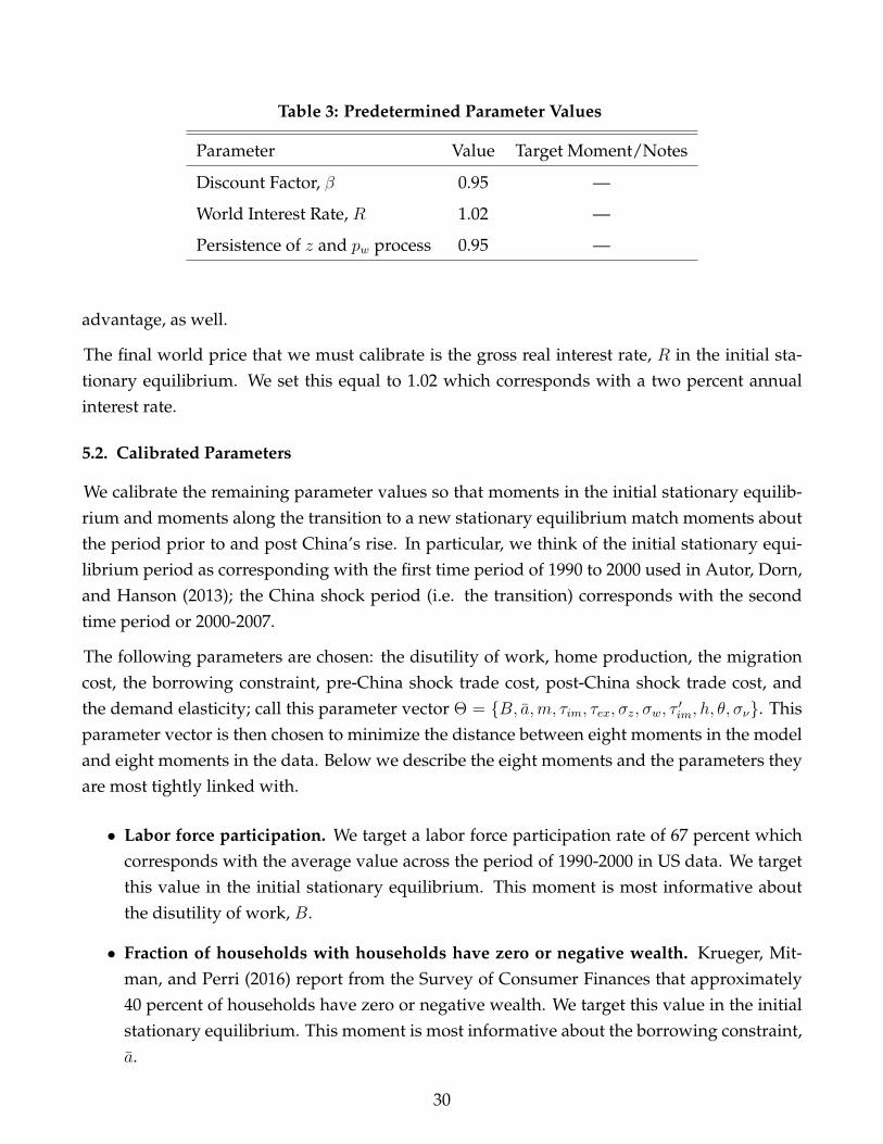
Table 3: Predetermined Parameter Values

Parameter Value Target Moment/Notes

Discount Factor, β 0.95 —

World Interest Rate, R 1.02 —

Persistence of z and pw process 0.95 —

advantage, as well.

The final world price that we must calibrate is the gross real interest rate, R in the initial sta-tionary equilibrium. We set this equal to 1.02 which corresponds with a two percent annualinterest rate.

5.2. Calibrated Parameters

We calibrate the remaining parameter values so that moments in the initial stationary equilib-rium and moments along the transition to a new stationary equilibrium match moments aboutthe period prior to and post China’s rise. In particular, we think of the initial stationary equi-librium period as corresponding with the first time period of 1990 to 2000 used in Autor, Dorn,and Hanson (2013); the China shock period (i.e. the transition) corresponds with the secondtime period or 2000-2007.

The following parameters are chosen: the disutility of work, home production, the migrationcost, the borrowing constraint, pre-China shock trade cost, post-China shock trade cost, andthe demand elasticity; call this parameter vector Θ = {B, a,m, τim, τex, σz, σw, τ ′im, h, θ, σν}. Thisparameter vector is then chosen to minimize the distance between eight moments in the modeland eight moments in the data. Below we describe the eight moments and the parameters theyare most tightly linked with.

• Labor force participation. We target a labor force participation rate of 67 percent whichcorresponds with the average value across the period of 1990-2000 in US data. We targetthis value in the initial stationary equilibrium. This moment is most informative aboutthe disutility of work, B.

• Fraction of households with households have zero or negative wealth. Krueger, Mit-man, and Perri (2016) report from the Survey of Consumer Finances that approximately40 percent of households have zero or negative wealth. We target this value in the initialstationary equilibrium. This moment is most informative about the borrowing constraint,a.

30

• Migration rate. We use the the IRS migration data which uses the address and reportedincome on individual tax filings to track how many individuals move in or out of a county.We compute that a bit over three percent of households move across a commuting zone ata yearly frequency. We target this value in the initial stationary equilibrium. This momentis most informative about the migration cost, m

• Trade volumes pre China’s rise. In the initial stationary equilibrium, we target an initialimport to GDP ratio of thirteen percent. This latter value is consistent with the degreeof openness seen in Figure 1 in the late 1990s prior to the acceleration of Chinese trade.This moment is most informative about the initial import and export trade cost (which weassume take on the same value initially).

• Standard deviation of growth rates in commute zone level labor earnings. In the initialstationary equilibrium, we target standard deviation of growth rates in commute zonelevel labor earnings of 6.5 percent. This value is measured in the data by using the de-cennial Census data from Autor, Dorn, and Hanson (2013) and focusing on the periodbetween 1990 and 2000. One short-cut that we take is that given in the closed economyversion of this model and given a ρ and θ, we can determine, in closed form, the volatilityof growth in labor earnings simply by picking σz. Thus, we directly calibrate this valueprior to computing the stationary equilibrium.

• Trade volumes post China’s rise. Along the transition path, we target an import to GDPratio of seventeen percent seven years after the change in policy. This latter value is con-sistent with the degree of openness seen in Figure 1 in 2007. This moment is most infor-mative about the final trade cost.

• Aggregate gains from trade. Given the long-run increase in trade from the bullet above,we can use the formula of Arkolakis, Costinot, and Rodrıguez-Clare (2012) to imputethe aggregate gain in output associated with a trade elasticity of four (Simonovska andWaugh (2014)). We then ensure that our model has the aggregate responses in outputas the Arkolakis, Costinot, and Rodrıguez-Clare (2012) would formula implies. Whilethe Arkolakis, Costinot, and Rodrıguez-Clare (2012) does formula does not hold in ourmodel, we are using their formula as a model diagnostic to ensuring that the level of thegains from trade are the same as in a standard, representative agent trade model.

This moment is most informative about the volatility of world prices, σw. This may seemodd, but read on. The insight here is that variation in world prices determines how elas-tic aggregate trade flows are to a change in trade frictions. For example, if world pricesare very dispersed, then large changes in trade frictions are necessary to generate largechanges in trade flows. In contrast, if if there is little variation in world prices, then small

31

changes in trade frictions will generate large changes in trade flows. This insight is anal-ogous to the behavior of the Eaton and Kortum (2002) model where the extent of technol-ogy heterogeneity controls how elastic trade flows are to changes in trade costs.

• Wage and labor force participation elasticity from Autor, Dorn, and Hanson (2013).Specifically, we target the elasticities described in Table 1. These moments are most in-formative about θ and wh. The logic about the relationship between the Autor, Dorn, andHanson’s (2013) wage elasticity result and θ and follows from the discussion in 4, that isthe elasticity of wages to changes in trade exposure is related to demand elasticity.

The home production parameter wh is related to the labor force participation elasticity ofAutor, Dorn, and Hanson (2013). The idea is that home production controls the opportu-nity cost of working in the market and, thus, it controls how households substitute in andout of the labor force in response to shocks. Given that Autor, Dorn, and Hanson (2013)have identified the elasticity of labor supply to a trade shock, this will inform our homeproduction parameter.

• Migration elasticity from Greenland, Lopresti, and McHenry (2017). We target theGreenland, Lopresti, and McHenry (2017) migration elasticity described in Table 2. Thismoments is most informative about the scale of the preference shock σν . For example, ifthe variance of the preference shocks are large, then large movements in the value of mov-ing relative to staying are required to induce households to move. On the other hand, ifthe variance of the shocks are small, then small changes in the relative value of moving tostaying will induce large numbers of households to move. Hence, the migration elasticityof Greenland, Lopresti, and McHenry (2017) helps pin this parameter down.

5.3. Implementing the China Shock

Main exercise focuses on a change in the the ability to import goods, i.e., a reduction in τim.Mechanically, we implement the change in the following way: In year one, the a new pathof trade costs are announced and implemented. The new, announced path of new trade coststhose that linearly decrease from τim to τ ′im over seven years. The idea here is to generate thegradual rise in trade as in the data and to mimic the narrative around the change trade policywith China’s accession to the WTO and granting of permanent normal trade relations by theUnited States. As mentioned above, the exact level of τ ′im is chosen so that after seven yearsfrom announcement, imports to GDP resemble that seen in the US in 2007.

5.4. The Procedure

To implement the calibration, we work through the following steps. Much of this is done in asimultaneous manner, but we describe the core steps to facilitate how we map our model into

32

the data.

Step 1. Guess the parameters σw, θ, wh, σν .

Step 2. We pick the parameters {B, a,m, τim, τex, σz} so that the initial stationary equilibrium(pre-China shock period) replicates the labor force participation rate, migration rate, net worthof households, volatility of labor earnings, and the initial volume of trade.

Step 3. We pick the parameter τ ′im and then compute the new stationary equilibrium. Wecompute the transition path. That is starting from the initial stationary distribution we changethe trade friction and compute the transition path to the new stationary distribution. We thencheck that seven years after the change, the volume of trade equals seventeen percent. Wecompute the long run aggregate gain in output and compare it to the value predicted by theArkolakis, Costinot, and Rodrıguez-Clare (2012) formula.

Step 4. Given the transition path, we simulate data sets analogous to those in Autor, Dorn,and Hanson (2013) and estimate the wage, labor force participation, and migration elasticitieswith respect to the trade exposure metric. In particular, we constructing data analogs in ourmodel as they are constructed in Autor, Dorn, and Hanson (2013) and estimate (2) on modelgenerated data with a time effect. Simulated trade flows for another country (same sequence ofpws, different sequence of zs) is the instrument.

Given the difference between the model and data elasticities, return to Step 1. and update theparameters σw, θ, wh, σν .

5.5. Calibration Results

Table 4 reports the calibration results parameters and the associated aggregate moments. Over-all, the model is very flexible and is easily able to exactly fit most moments. The only momentsin which there is some minor difficult are those that depend upon the transition path. At thecurrent stage, this appears to be largely due to time constraints and the solver needing moretime to find the exact parameterizations.

Figure 7 plots the model’s prediction for imports. Similar to the data, the model generates risingtrade exposure over the early 2000s. As we discuss below, one feature of the model is that oncethe path of trade costs are announced, consumption contracts by a small amount. Since demandfor all goods (including imported) are contracting, imports fall by a slight amount in the firstcouple of years and then slowly rise.

Table 5 reports the micro-moments, model prediction/fit, and the resulting parameter values.The first row reports the estimates from Autor, Dorn, and Hanson (2013) and Greenland, Lo-presti, and McHenry (2017), the second row reports the results from the calibrated model. Thereare a couple of points to mention. First, our model is able to come in the close vicinity the

33

Table 4: Calibration: Parameters and Aggregate Moments

Parameter Value Target Data Model

Disutility of work, B 1.05 Aggregate participation rate 66 66

Migration Cost, m 1.75 CMZ. migration rate 3 3

Borrowing Limit, −a 0.84 % Households with ≤ 0 net worth 40 40

Pre-China Trade Cost (τex, τim) 1.16 1990s Imports/GDP 13 13

Post-China Trade Cost (τ ′im) 1.37 2007 Imports/GDP 16.2 15.4

Std. Dv. of z (σz) 0.032 Std. Dev. in CMZ earnings 7 9

Std. Dv. of pw (σw) 1.64×σz Predicted ACR Gains 1.6 1.8

Note: All moments are reported in percent. Migration cost and borrowing limit parameters are reported asa fraction of output per worker.

micro-moments. All point estimates from the model lie within the 95-5 confidence bands ofthe data. Our interpretation of this (along with extensive sensitivity analysis) is that results ofAutor, Dorn, and Hanson (2013) are informative about structural parameters that govern theunderlying data generating process.

With that said, the model is experiencing difficulty in exactly nailing these moments. Thedifficulty appears to be in the strong substitution pattern between not working and migrating.In the model, households are unseing these two margins to avoid the negative consequencesof the shock. And when one of the margins looks more or less favorable, the model impliedelasticities change in different ways.

A final point of note is that the estimated demand elasticity, θ, is relatively large. The reasonfollows from the discussion in Section 4: The elasticity of wages to changes in trade exposureis related to one over the demand elasticity. So if the demand elasticity is high, then changes intrade exposure will weakly pass-through into wages. Hence, what this is telling us vis-a-vi theAutor, Dorn, and Hanson (2013) evidence, is that pass-through was not that strong.

6. The China Trade Shock

This section analyzes the affects of a change in the ability to import goods on the economy atthe macro and micro level.

34

1999 2000 2001 2002 2003 2004 2005 2006 2007Time

11

12

13

14

15

16

17

Perc

enta

ge o

f GDP

Imports / GDP

ModelData

Figure 7: Rising Trade Exposure: Model and Data

6.1. The China Shock at the Micro level

As a first step to understanding the aggregate and welfare effects of the shock, we take a deeperlook “under the hood“ at how real wages, labor supply, and consumption respond at the islandlevel.

Real Wages. Figure 8 plots the log change in real wages across islands six years after the shock.The islands are ordered from the left to right by initial trade exposure with those to the left (andred colored) being import exposed. The pattern of change looks a bit bizarre, but with a littleeffort it makes complete sense and leads to several surprising insights.

First consider the exporting region (blue, positive bars to the right). These islands experiencelarge gains in real wages—nearly four percent. Where does the gain come from and why isit same across exporting islands? Real wages increase through increases in real purchasingpower, i.e. the decline in the CES price index. And because this effect is common across allexporting regions, they receive the same proportional gain. To see this point, recall that wages

35

Table 5: Calibration: Micro Moments and Parameters

∆ Labor Earnings ∆ NILF GLM ∆ Population

Data −4.30

[−6.62, −2.00]

1.11

[0.52, 1.72]

−1.43

[−3.33, 0.48]

Model −4.10 1.24 −1.92

Demand elasticity θ Home production wh Moving shock variance σν

Parameter Values 9.53 0.22 0.96

Note: Values in brackets report 95-5 confidence intervals.

in this region are such that

w(s) =pwz

τexP.

For a given island type, only the CES price index P changes and these is why those in theexporting region gain.

Now consider the importing region (red, positive bars to the right). This region experienceslarge declines in real wages, nearly two percent. Why the loss and why is it same across importexposed islands? The loss is from the decline in world prices (inclusive of trade costs) net of thegain in purchasing power. To see this point, wages for a given island type are:

w(s) =τimpwz

P.

Two forces work in the opposite direction: one is the decline in the trade cost, effective worldprices are falling. The second force is the rise in real purchasing power, i.e. the decline in theCES price index. Given the discussion above, the fall in the CES price index can be inferred bythe effects on the exporting region, a four percent decline. This implies that trade costs fall bysix percent and, on net, households in these regions experience a two percentage point drop inreal wages.

Finally, consider the non-traded region (black, in the middle). In this region real wages arerelatively unchanged. This may seem strange—we just argued that real purchasing power isincreasing and these goods are not exposed to trade. Why are real wages not increasing? Theissue is that the reduction in the CES price index from trade leads consumers to substitute away

36

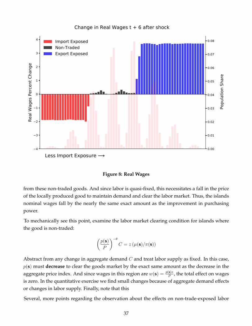
4

3

2

1

0

1

2

3

4

Real

Wag

es P

erce

nt C

hang

e

Less Import Exposure

Change in Real Wages t + 6 after shock

Import ExposedNon-TradedExport Exposed

0.00

0.01

0.02

0.03

0.04

0.05

0.06

0.07

0.08

Pop

ulat

ion

Shar

e

Figure 8: Real Wages

from these non-traded goods. And since labor is quasi-fixed, this necessitates a fall in the priceof the locally produced good to maintain demand and clear the labor market. Thus, the islandsnominal wages fall by the nearly the same exact amount as the improvement in purchasingpower.

To mechanically see this point, examine the labor market clearing condition for islands wherethe good is non-traded: (

p(s)

P

)−θC = z (µ(s)/π(s))

Abstract from any change in aggregate demand C and treat labor supply as fixed. In this case,p(s) must decrease to clear the goods market by the exact same amount as the decrease in theaggregate price index. And since wages in this region are w(s) = p(s)z

P, the total effect on wages

is zero. In the quantitative exercise we find small changes because of aggregate demand effectsor changes in labor supply. Finally, note that this

Several, more points regarding the observation about the effects on non-trade-exposed labor

37

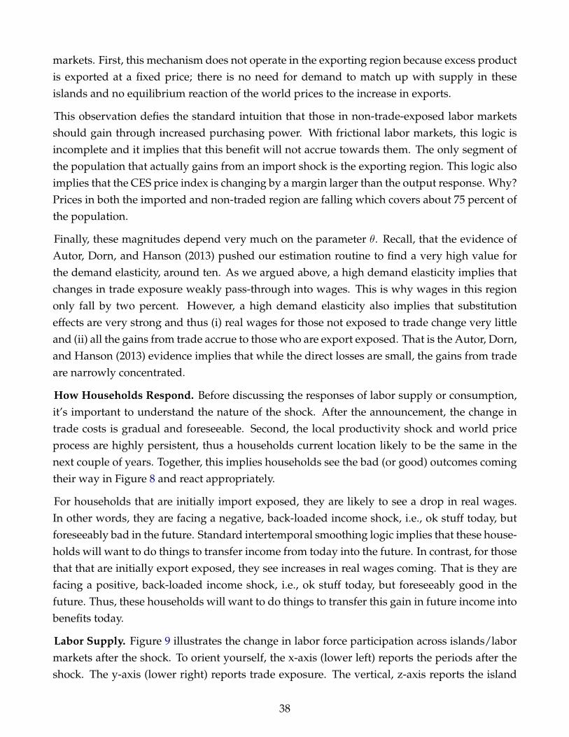
markets. First, this mechanism does not operate in the exporting region because excess productis exported at a fixed price; there is no need for demand to match up with supply in theseislands and no equilibrium reaction of the world prices to the increase in exports.

This observation defies the standard intuition that those in non-trade-exposed labor marketsshould gain through increased purchasing power. With frictional labor markets, this logic isincomplete and it implies that this benefit will not accrue towards them. The only segment ofthe population that actually gains from an import shock is the exporting region. This logic alsoimplies that the CES price index is changing by a margin larger than the output response. Why?Prices in both the imported and non-traded region are falling which covers about 75 percent ofthe population.

Finally, these magnitudes depend very much on the parameter θ. Recall, that the evidence ofAutor, Dorn, and Hanson (2013) pushed our estimation routine to find a very high value forthe demand elasticity, around ten. As we argued above, a high demand elasticity implies thatchanges in trade exposure weakly pass-through into wages. This is why wages in this regiononly fall by two percent. However, a high demand elasticity also implies that substitutioneffects are very strong and thus (i) real wages for those not exposed to trade change very littleand (ii) all the gains from trade accrue to those who are export exposed. That is the Autor, Dorn,and Hanson (2013) evidence implies that while the direct losses are small, the gains from tradeare narrowly concentrated.

How Households Respond. Before discussing the responses of labor supply or consumption,it’s important to understand the nature of the shock. After the announcement, the change intrade costs is gradual and foreseeable. Second, the local productivity shock and world priceprocess are highly persistent, thus a households current location likely to be the same in thenext couple of years. Together, this implies households see the bad (or good) outcomes comingtheir way in Figure 8 and react appropriately.

For households that are initially import exposed, they are likely to see a drop in real wages.In other words, they are facing a negative, back-loaded income shock, i.e., ok stuff today, butforeseeably bad in the future. Standard intertemporal smoothing logic implies that these house-holds will want to do things to transfer income from today into the future. In contrast, for thosethat that are initially export exposed, they see increases in real wages coming. That is they arefacing a positive, back-loaded income shock, i.e., ok stuff today, but foreseeably good in thefuture. Thus, these households will want to do things to transfer this gain in future income intobenefits today.

Labor Supply. Figure 9 illustrates the change in labor force participation across islands/labormarkets after the shock. To orient yourself, the x-axis (lower left) reports the periods after theshock. The y-axis (lower right) reports trade exposure. The vertical, z-axis reports the island

38

level change in labor force participation.

Those islands that are initially import exposed (red and to the left on the y-axis) initially in-crease their labor supply by a substantial margin, almost four percentage points for the mostexposed. Households on these islands see the negative effects coming and use labor supply tofulfill their intertemporal savings motives. That is work hard today to build up savings andfacilitate the smoothing out of the foreseen, future negative income shock. As the shock pro-gresses, this desire partially dissipates and labor force participation is one percent higher forimport exposed islands.

In contrast, those that are export exposed (blue and to the right on the y-axis) decrease theirlabor supply. Households on these islands see the gains from trade coming their way. Andthus they transfer some of this new found wealth into benefits today by substituting into leisure.And this effect dissipates as households eventually increasing their labor supply as the benefitsfrom participating in the labor market become increasingly generous. That is because of therise in wages seen in Figure 8, their opportunity cost of not working increases and this inducesparticipation.

Consumption/Savings. Figure 10 illustrates the change in island-level savings rates. Every-thing here is the same as Figure 9, except now the vertical, z-axis reports the percentage pointchange in the island level savings rate. The savings rate is simply the one minus island levelconsumption relative to island level labor income (wages multiplied by labor supply). Thisis crude and hides a lot of heterogeneity, but it provides a picture of the change in savingsbehavior.

In many ways, Figure 10 mimics the patterns in labor supply. Import exposed islands are facinga negative, back-loaded income shock and want to find ways to transfer income today intothe future to mitigate the foreseen, future negative income shock. In contrast, export exposedislands who foresee increases in real wages increase their consumption today and decrease theirsavings to transfer future benefits into today.

Long Run Outcomes. Figures 9 and 10 also illustrate that these patterns reverse as the econ-omy approaches the new stationary equilibrium. Export exposed islands tend to participatemore and save more; import exposed islands tend participate less and save less. Moreover, theislands in the middle (which are non-traded regions) which work and save at the highest rates.

Precautionary motives drive this behavior. In the model, a reduction in trade costs increasesthe amount of uninsurable income risk in the model. The idea here is that while many house-holds are not directly exposed, a reduction in trade costs increases the likelihood that they willeventually become trade exposed and, thus trade leads to an increase in income risk. This forceincreases precautionary savings motives (see, e.g., Huggett and Ospina (2001)) and leads to anincrease in labor supply to acquire income and a higher savings rate.

39

Years After Shock

12

34

56

78

910

Initial Trade Exposure:

Less Import Exposure

Cha

nge

in L

FP

8

6

4

2

0

2

4

6

8

Figure 9: Model: Change in Labor Supply, Across Islands

Years After Shock

12

34

56

78

910

Initial Trade Exposure:

Less Import Exposure

Cha

nge

in S

avin

gs R

ate

15

10

5

0

5

10

Figure 10: Model: Change in Savings, Across Islands

40

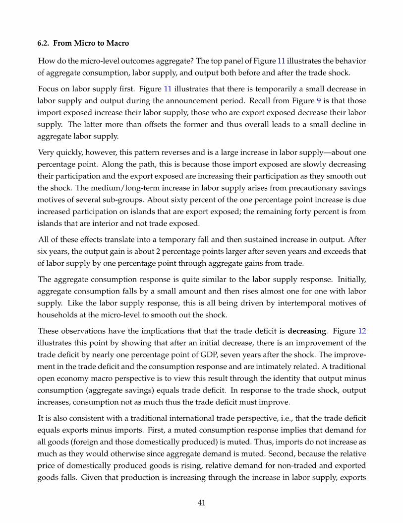
6.2. From Micro to Macro

How do the micro-level outcomes aggregate? The top panel of Figure 11 illustrates the behaviorof aggregate consumption, labor supply, and output both before and after the trade shock.

Focus on labor supply first. Figure 11 illustrates that there is temporarily a small decrease inlabor supply and output during the announcement period. Recall from Figure 9 is that thoseimport exposed increase their labor supply, those who are export exposed decrease their laborsupply. The latter more than offsets the former and thus overall leads to a small decline inaggregate labor supply.

Very quickly, however, this pattern reverses and is a large increase in labor supply—about onepercentage point. Along the path, this is because those import exposed are slowly decreasingtheir participation and the export exposed are increasing their participation as they smooth outthe shock. The medium/long-term increase in labor supply arises from precautionary savingsmotives of several sub-groups. About sixty percent of the one percentage point increase is dueincreased participation on islands that are export exposed; the remaining forty percent is fromislands that are interior and not trade exposed.

All of these effects translate into a temporary fall and then sustained increase in output. Aftersix years, the output gain is about 2 percentage points larger after seven years and exceeds thatof labor supply by one percentage point through aggregate gains from trade.

The aggregate consumption response is quite similar to the labor supply response. Initially,aggregate consumption falls by a small amount and then rises almost one for one with laborsupply. Like the labor supply response, this is all being driven by intertemporal motives ofhouseholds at the micro-level to smooth out the shock.

These observations have the implications that that the trade deficit is decreasing. Figure 12illustrates this point by showing that after an initial decrease, there is an improvement of thetrade deficit by nearly one percentage point of GDP, seven years after the shock. The improve-ment in the trade deficit and the consumption response and are intimately related. A traditionalopen economy macro perspective is to view this result through the identity that output minusconsumption (aggregate savings) equals trade deficit. In response to the trade shock, outputincreases, consumption not as much thus the trade deficit must improve.

It is also consistent with a traditional international trade perspective, i.e., that the trade deficitequals exports minus imports. First, a muted consumption response implies that demand forall goods (foreign and those domestically produced) is muted. Thus, imports do not increase asmuch as they would otherwise since aggregate demand is muted. Second, because the relativeprice of domestically produced goods is rising, relative demand for non-traded and exportedgoods falls. Given that production is increasing through the increase in labor supply, exports

41

1999 2000 2001 2002 2003 2004 2005 2006 2007Time

98

99

100

101

102

103Va

lues

Rel

ativ

e to

Initi

al S

S Model: GDP, Consumption, and Labor Supply

GDPConsumptionLabor Supply

Figure 11: Model: Consumption, Output, Labor Supply

1999 2000 2001 2002 2003 2004 2005 2006 2007Time

1.0

0.5

0.0

0.5

1.0

1.5

Perc

enta

ge P

oint

Cha

nge

From

Bas

elin

e

Model: Trade Imbalance (NX / GDP)

Figure 12: Trade Defect42

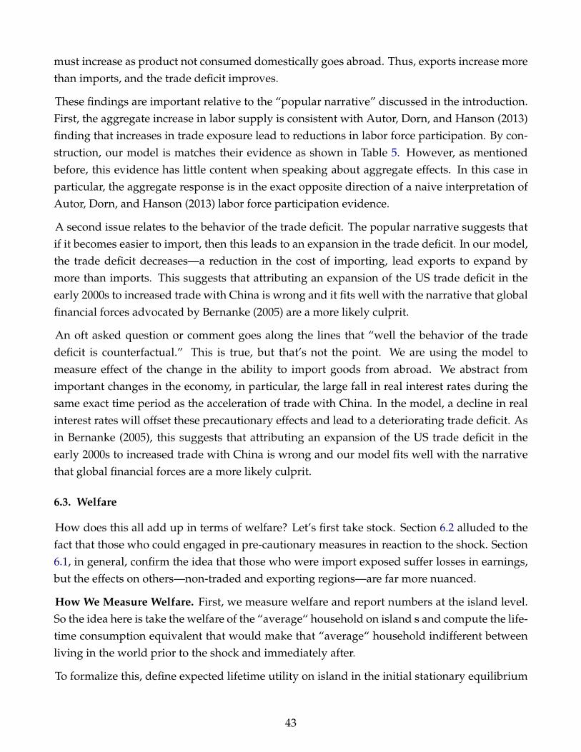
must increase as product not consumed domestically goes abroad. Thus, exports increase morethan imports, and the trade deficit improves.

These findings are important relative to the “popular narrative” discussed in the introduction.First, the aggregate increase in labor supply is consistent with Autor, Dorn, and Hanson (2013)finding that increases in trade exposure lead to reductions in labor force participation. By con-struction, our model is matches their evidence as shown in Table 5. However, as mentionedbefore, this evidence has little content when speaking about aggregate effects. In this case inparticular, the aggregate response is in the exact opposite direction of a naive interpretation ofAutor, Dorn, and Hanson (2013) labor force participation evidence.

A second issue relates to the behavior of the trade deficit. The popular narrative suggests thatif it becomes easier to import, then this leads to an expansion in the trade deficit. In our model,the trade deficit decreases—a reduction in the cost of importing, lead exports to expand bymore than imports. This suggests that attributing an expansion of the US trade deficit in theearly 2000s to increased trade with China is wrong and it fits well with the narrative that globalfinancial forces advocated by Bernanke (2005) are a more likely culprit.

An oft asked question or comment goes along the lines that “well the behavior of the tradedeficit is counterfactual.” This is true, but that’s not the point. We are using the model tomeasure effect of the change in the ability to import goods from abroad. We abstract fromimportant changes in the economy, in particular, the large fall in real interest rates during thesame exact time period as the acceleration of trade with China. In the model, a decline in realinterest rates will offset these precautionary effects and lead to a deteriorating trade deficit. Asin Bernanke (2005), this suggests that attributing an expansion of the US trade deficit in theearly 2000s to increased trade with China is wrong and our model fits well with the narrativethat global financial forces are a more likely culprit.

6.3. Welfare

How does this all add up in terms of welfare? Let’s first take stock. Section 6.2 alluded to thefact that those who could engaged in pre-cautionary measures in reaction to the shock. Section6.1, in general, confirm the idea that those who were import exposed suffer losses in earnings,but the effects on others—non-traded and exporting regions—are far more nuanced.

How We Measure Welfare. First, we measure welfare and report numbers at the island level.So the idea here is take the welfare of the “average“ household on island s and compute the life-time consumption equivalent that would make that “average“ household indifferent betweenliving in the world prior to the shock and immediately after.

To formalize this, define expected lifetime utility on island in the initial stationary equilibrium

43

as

W (s;χ(s)) =

∫a

∫ν

V (a, s, ν;χ(s))λ(s, a, ν) dν da, (33)

where χ is the consumption equivalent parameter. Welfare immediately after the shock is

W ′(s) =

∫a

∫ν

V ′(a, s, ν)λ′(s, a, ν) dν da. (34)

Thus, our measure of welfare is the value of χ(s) which must make W (s;χ(s)) = W ′(s). Onepoint to notice that this measure hides the heterogeneity of households within an islands. Be-cause each island has its own distribution of assets, there is variation in how much a householdon that island wins (or loses). By integrating over asset holdings within an island, we are notexploring this variation.

Welfare Effects of the Shock Table 6 summarizes our findings in addition to reporting thechange in real wages; Figure 13 illustrates the full range of outcomes by plotting the welfaregains for each island type.

On average, the gains are not out-of-line with what a simple calculation from Arkolakis, Costinot,and Rodrıguez-Clare (2012) would suggest. A little less than one percentage point which moreor less matches up with the average change in real wages which is a bit more than one percent.

Table 6: Welfare

Welfare (Baseline) ∆ Real Wages

Average 0.94 1.06

Init

ialE

xpos

ure Import Exposed 0.19

[ 0.09 ]

−2.19

[ 0.09 ]

Non-Traded 0.75

[ 0.68 ]

0.34

[ 0.68 ]

Export Exposed 1.64

[ 0.25 ]

3.99

[ 0.25 ]

Note: Valeus are lifetime consumption equivalents; values in brackets re-port the share of the population in that catagory.

The interesting outcomes are with respect to the distributional consequences. First, as Figure13 shows, those who are initially import exposed experience welfare loses, though some ex-

44

1

0

1

2

3

Wel

fare

, CE

Units

in P

erce

nt

Less Import Exposure

Welfare: Trade ShockAverage WelfareImport ExposedNon-TradedExport Exposed

0.00

0.01

0.02

0.03

0.04

0.05

0.06

0.07

0.08

Initi

al P

opul

atio

n Sh

are

Figure 13: Welfare Across Islands

perience very small, but positive gains. A few losses, minor gains, stands in sharp contrast tothe harsh effects trade has on these labor market outcomes—wages falling by two percentagepoints over the first five years of the shock. As alluded to above, the disconnect between wageoutcomes and welfare arises from households actively using margins of adjustment to mitigatethe effects of the shock. Import exposed households increase their labor supply to build upsavings and smooth out the foreseen, future negative income shock from China.

Surprisingly those that are in non-traded regions experience substantial welfare gains, about0.75 percent increase in welfare. As argued above, these households experience essentially nochange in real wages as two forces counteract each other: while the real purchasing power in-creases for these households, the value of the goods produced by these households also fallsas consumers substitute into cheaper imported goods. In welfare terms, these householdsstill gain but These are dynamic gains which arise from the stochastic nature of comparativeadvantage—that at some point they will be in a situation that comparative advantage favorsthem and they reap the benefits.

Finally, those in the exporting regions gain the most, a bit less than two percent. Recall several

45

points discussed above. First, these gains are purely through changes in the price index and,hence, a rise in real wages. Second, the change in real wages does not map one for one into wel-fare for several reasons. These are transitory gains relative to the average and, thus, a portionof this is simply saved for possible bad times in the future. Moreover, relative bad times in thefuture will come and, thus, their inviable position is merely transitory.

6.4. The role of the Autor, Dorn, and Hanson (2013) evidence

The evidence of Autor, Dorn, and Hanson (2013) is central to disciplining the small negativewelfare effects from trade seen in Figure 13. We illustrate this point by showing what patternsin the data would suggest larger welfare losses from trade. We proceed by re-calibrating themodel to match all the same moments, except target a larger wage elasticity of -8.60 rather than-4.30 as in seen the data.

The top two lines of the Table 7 report the key calibration outcomes from this exercise. Weare easily able to match the higher wage elasticity of -8.60. All other moments are essentiallythe same as reported above. The second line of Table 7 reports the demand elasticity. As ar-gued above this is the key parameter for which the wage elasticity is informative about and isthe parameter. Here the demand elasticity is near five—half the value found in our baselinecalibration with the value of ten.

Because this calibration results in a smaller elasticity of substitution across goods and thechange in the volume of trade is the same, the implication is that there is a stronger pass-through of the trade shock into wages. The right most column reports the change in real wagesacross different exposure to trade. Here wages fall by more for the import exposed; those in themiddle experience literally no change; and those at the top experience smaller wage gains. Sothis parameterizations essentially results in more losers, less winners in terms of labor earnings.Welfare essentially mimics the same patter, but with the losses from trade being small.

7. Final Thoughts

Researchers with more experience than us have remarked to us in (sometimes in a semi-pejorativeway) the following: “We know that the standard incomplete market model gives outcomeswhich are in, welfare terms, near a complete markets benchmark.” Well that’s the point—takethe evidence of Autor, Dorn, and Hanson (2013) and give households limited, but some self-insurance mechanisms and the interpretation about the negative effects from trade completelychange. With that said, our paper is a starting point that suggests where to look if our prior isthat trade had negative consequences. One area to explore are different financial market fric-tions, specifically housing wealth or forms of liquid and non-liquid wealth (e.g., Kaplan andViolante (2014)).

46

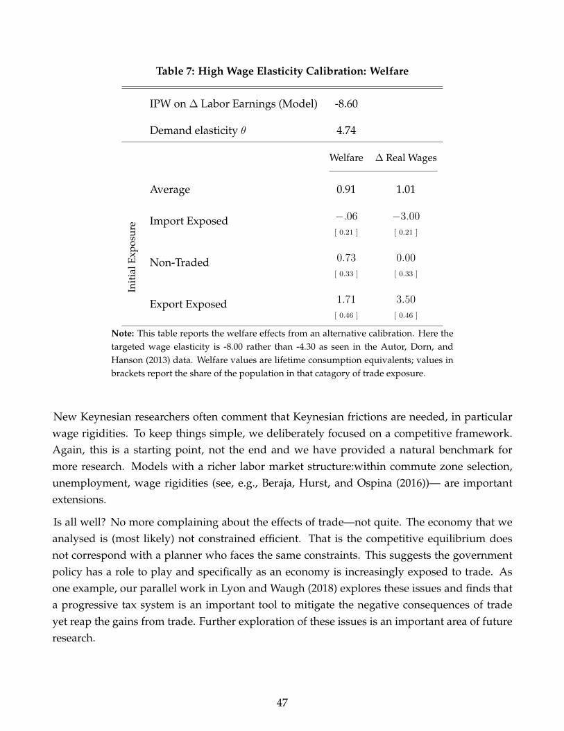
Table 7: High Wage Elasticity Calibration: Welfare

IPW on ∆ Labor Earnings (Model) -8.60

Demand elasticity θ 4.74

Welfare ∆ Real Wages

Average 0.91 1.01

Init

ialE

xpos

ure Import Exposed −.06

[ 0.21 ]

−3.00

[ 0.21 ]

Non-Traded 0.73

[ 0.33 ]

0.00

[ 0.33 ]

Export Exposed 1.71

[ 0.46 ]

3.50

[ 0.46 ]

Note: This table reports the welfare effects from an alternative calibration. Here thetargeted wage elasticity is -8.00 rather than -4.30 as seen in the Autor, Dorn, andHanson (2013) data. Welfare values are lifetime consumption equivalents; values inbrackets report the share of the population in that catagory of trade exposure.

New Keynesian researchers often comment that Keynesian frictions are needed, in particularwage rigidities. To keep things simple, we deliberately focused on a competitive framework.Again, this is a starting point, not the end and we have provided a natural benchmark formore research. Models with a richer labor market structure:within commute zone selection,unemployment, wage rigidities (see, e.g., Beraja, Hurst, and Ospina (2016))— are importantextensions.

Is all well? No more complaining about the effects of trade—not quite. The economy that weanalysed is (most likely) not constrained efficient. That is the competitive equilibrium doesnot correspond with a planner who faces the same constraints. This suggests the governmentpolicy has a role to play and specifically as an economy is increasingly exposed to trade. Asone example, our parallel work in Lyon and Waugh (2018) explores these issues and finds thata progressive tax system is an important tool to mitigate the negative consequences of tradeyet reap the gains from trade. Further exploration of these issues is an important area of futureresearch.

47

References

ACEMOGLU, D., D. AUTOR, D. DORN, G. H. HANSON, AND B. PRICE (2016): “Import com-petition and the great US employment sag of the 2000s,” Journal of Labor Economics, 34(S1),S141–S198.

ACEMOGLU, D., AND P. RESTREPO (2017): “Robots and Jobs: Evidence from US Labor Mar-kets,” Discussion paper, National Bureau of Economic Research.

AIYAGARI, S. R. (1994): “Uninsured idiosyncratic risk and aggregate saving,” The QuarterlyJournal of Economics, 109(3), 659–684.

ARKOLAKIS, C., A. COSTINOT, AND A. RODRIGUEZ-CLARE (2012): “New Trade Models, SameOld Gains?,” American Economic Review, 102(1), 94–130.

ARTUC, E., S. CHAUDHURI, AND J. MCLAREN (2010): “Trade shocks and labor adjustment: Astructural empirical approach,” The American Economic Review, 100(3), 1008–1045.

AUTOR, D., D. DORN, AND G. H. HANSON (2013): “The China Syndrome: Local Labor MarketEffects of Import Competition in the United States,” The American Economic Review, 103(6),2121–2168.

BERAJA, M., E. HURST, AND J. OSPINA (2016): “The aggregate implications of regional businesscycles,” Discussion paper, National Bureau of Economic Research.

BERNANKE, B. (2005): “The global saving glut and the US current account deficit,” Discussionpaper.

CALIENDO, L., M. A. DVORKIN, AND F. PARRO (2015): “Trade and labor market dynamics,” .

CHANG, Y., AND S.-B. KIM (2007): “Heterogeneity and aggregation: Implications for labor-market fluctuations,” The American Economic Review, 97(5), 1939–1956.

CHARLES, K. K., E. HURST, AND M. J. NOTOWIDIGDO (2016): “The masking of the declinein manufacturing employment by the housing bubble,” The Journal of Economic Perspectives,30(2), 179–200.

COSAR, A. K., N. GUNER, AND J. TYBOUT (2016): “Firm dynamics, job turnover, and wagedistributions in an open economy,” The American Economic Review, 106(3), 625–663.

DIX-CARNEIRO, R. (2014): “Trade liberalization and labor market dynamics,” Econometrica,82(3), 825–885.

DIXIT, A. (1987): “Trade and insurance with moral hazard,” Journal of international economics,23(3-4), 201–220.

48

(1989a): “Trade and Insurance with Adverse Selection,” The Review of Economic Studies,56(2), 235–247.

(1989b): “Trade and Insurance with Imperfectly Observed Outcomes,” The QuarterlyJournal of Economics, 104(1), 195–203.

DORNBUSCH, R., S. FISCHER, AND P. A. SAMUELSON (1977): “Comparative advantage, trade,and payments in a Ricardian model with a continuum of goods,” The American EconomicReview, 67(5), 823–839.

EATON, J., AND G. M. GROSSMAN (1985): “Tariffs as Insurance: Optimal Commercial PolicyWhen Domestic Markets Are Incomplete,” The Canadian Journal of Economics / Revue canadi-enne d’Economique, 18(2), 258–272.

EATON, J., AND S. KORTUM (2002): “Technology, geography, and trade,” Econometrica, 70(5),1741–1779.

GREENLAND, A., J. LOPRESTI, AND P. MCHENRY (2017): “Import competition and internalmigration,” .

HANSON, G. H., N. LIND, AND M.-A. MUENDLER (2015): “The dynamics of comparativeadvantage,” Discussion paper, National Bureau of Economic Research.

HUGGETT, M. (1993): “The risk-free rate in heterogeneous-agent incomplete-insuranceeconomies,” Journal of economic Dynamics and Control, 17(5), 953–969.

HUGGETT, M., AND S. OSPINA (2001): “Aggregate precautionary savings: when is the thirdderivative irrelevant?,” Journal of Monetary Economics, 48(2), 373–396.

JONES, C., V. MIDRIGAN, AND T. PHILIPPON (2018): “Household Leverage and the Recession,”Discussion paper, National Bureau of Economic Research.

KAMBOUROV, G. (2009): “Labour Market Regulations and the Sectoral Reallocation of Workers:The Case of Trade Reforms,” Review of Economic Studies, 76(4), 1321–1358.

KAPLAN, G., AND G. L. VIOLANTE (2014): “A model of the consumption response to fiscalstimulus payments,” Econometrica, 82(4), 1199–1239.

KRISHNA, P., AND M. Z. SENSES (2014): “International Trade and Labour Income Risk in theU.S.,” The Review of Economic Studies, 81(1), 186–218.

KRUEGER, D., K. MITMAN, AND F. PERRI (2016): “Macroeconomics and Household Hetero-geneity,” Handbook of Macroeconomics, 2, 843–921.

49

KRUSELL, P., T. MUKOYAMA, AND A. SAHIN (2010): “Labour-market matching with precau-tionary savings and aggregate fluctuations,” The Review of Economic Studies, 77(4), 1477–1507.

LUCAS, R. E., AND E. C. PRESCOTT (1974): “Equilibrium search and unemployment,” Journalof Economic Theory, 7(2), 188–209.

LYON, S., AND M. WAUGH (2018): “Redistributing the Gains From Trade Through ProgressiveTaxation,” .

MIAN, A., K. RAO, AND A. SUFI (2013): “Household Balance Sheets, Consumption, and theEconomic Slump*.,” Quarterly Journal of Economics, 128(4).

MIAN, A., AND A. SUFI (2014): “What explains the 2007–2009 drop in employment?,” Econo-metrica, 82(6), 2197–2223.

MIRANDA, M. J., AND P. L. FACKLER (2004): Applied computational economics and finance.

MORTEN, M. (2016): “Temporary migration and endogenous risk sharing in village india,”Discussion paper, National Bureau of Economic Research.

NAKAMURA, E., AND J. STEINSSON (2014): “Fiscal stimulus in a monetary union: Evidencefrom US regions,” American Economic Review, 104(3), 753–92.

NAKAMURA, E., AND J. STEINSSON (2018): “Identification in macroeconomics,” Journal of Eco-nomic Perspectives, 32(3), 59–86.

NEWBERY, D. M., AND J. E. STIGLITZ (1984): “Pareto inferior trade,” The Review of EconomicStudies, 51(1), 1–12.

ROGERSON, R. (1988): “Indivisible labor, lotteries and equilibrium,” Journal of monetary Eco-nomics, 21(1), 3–16.

SIMONOVSKA, I., AND M. E. WAUGH (2014): “The Elasticity of Trade: Estimates and Evidence,”Journal of International Economics, 92(1), 34–50.

TOLBERT, C. M., AND M. SIZER (1996): “US commuting zones and labor market areas: A 1990update,” .

50

A. Connection with National Accounts

This section connects these equilibrium relationships to national income and product accounts(NIPA). This will help facilitate an understanding of the connection between trade imbalancesand household’s consumption-savings decisions. Note that in all of this derivation, we normal-ize the price of the final good to one.

The Income Side of NIPA. It is first useful to start from an income side measure of produc-tion (or GDP) in our economy. Given competition, the value of aggregate production of thefinal good must equal aggregate payments for intermediate goods. The latter equals aggregatepayments to labor in the production of all intermediate goods.

Y =

∫sw(s)µ(s) (35)

Examining (??) and (35) allows us to connect aggregate income with consumption. Specifically,by integrating over the consumers budget constraint (ignoring home production), then notinghow total value added must equal wages, one can substitute (35) into (??), then we arrive at thefollowing:

Y = C −RA+A′ +∫a

∫smιm(s, a)λ(s, a) (36)

so aggregate income equals consumption (private and public) minus (i) returns on assets (ii)new purchases of assets (iii) plus moving costs.

This basically says that income/production must equal consumption net of income not associ-ated with production (i.e. returns on assets) plus “investment” in assets and moving costs. Forexample, if consumption is larger than income one reason is that (in aggregate) households (onnet) are borrowing from abroad (A′ < 0).

Production Side of NIPA. The the value of aggregate production of the final good must equalthe value of intermediate goods production

Y =

∫sp(s)zµ(s) (37)

which we can then connect with the expenditure side of GDP through the market clearingconditions for intermediate goods and final goods. Specifically, by connecting the productionside with the demand side for non-traded goods in (19), imports in (21) and exports in (23) and

51

the equating final demand with consumption we have

Y = C +

∫sp(s)exports(s)−

∫sp(s)imports(s). (38)

Or GDP equals consumption (market) plus exports minus imports.

Savings, Trade Imbalances, and Capital Flows. Finally, we can connect the income side andthe production side the national accounts to arrive at a relationship between asset holdings andtrade imbalances. By working with both (36) and (38) we get the following relationship

Y− C =

∫sp(s)exports(s)−

∫sp(s)imports(s), (39)

=− rA+ (A′ −A) +

∫a

∫smιm(s, a)λ(s, a),

where r is the net real interest rate. This relationship says the following: aggregate savingsequals the trade imbalance. And this, in turn, we can connect the trade balance with the savingsdecisions of the households. That is the trade balance equals payments on net asset holdingsplus net change in asset holdings (adjusted for moving costs). To map this into Balance ofPayments language: the trade imbalance plus foreign income payments is the current account;the capital account is the net change in foreign asset holdings; then (we suspect) moving costswould show up as the “balancing item.”

To see this, consider the special case where moving costs are zero, no home production, andtariffs are zero. Then we have the relationship

Y − C =

∫sp(s)exports(s)−

∫sp(s)imports(s) = −rA+ (A′ −A). (40)

Here if exports are greater than imports, then this implies that the households are doing severalthings. The trade surplus may reflect that households (on net) are making debt payments (rA isnegative). Second, the trade surplus may reflect that the households (on net) are acquiring for-eign assets (A′−A is positive). Finally, note that in a stationary equilibrium, the trade imbalanceonly reflects payments from foreign asset holdings. This implies that the current account andcapital account are always zero in a stationary equilibrium, but that trade may be imbalanced.

52

B. Computational Appendix

This section describes our computational approach. Related materials are posted at https://github.com/mwaugh0328/redistributing_gains_from_trade which retains codefor our companion paper in Lyon and Waugh (2018). The code is presented in two differentlanguages: Matlab and Julia. The implementation in both languages follows the same coresteps, but the details are slightly different. The discussion below follows the Matlalb code. Fora detailed explanation of how the Julia code works, see the file julia/README Julia.md.

2.1. Computing and Solving the Stationary Equilibrium

Below we describe how to compute and solve the stationary equilibrium of the model.

• We approximate the continuous asset, productivity, and world price states by discretiza-tion. The asset space follows a non-uniform grid with grid points clustered near the bor-rowing constraint. The number of grid points was set to 50; the results are not sensitive toincreases in this number. We use the method of Rouwenhorst to discretize the productiv-ity and world price process. We use 10 states for productivity and world prices each, thusthere are 100 different states s.

• Guess a proposed price function p(s).

• Compute wages.

• Solve the households problem in (9). This is performed using value function iteration.

One technique we use to facilitate finding a solution to the equilibrium is to “smooth”out the discrete choice problem. We do this by assuming that there are additive logisti-cally distributed preference shocks with parameter bsmth and these preference shocks areindependently distributed across each choice. These enter into the choice problem in (9)by adding onto each option. What this gives rise to is, for each asset holdings state andstate s, there will be a non-zero mass of households choosing all options. The probabili-ties take the familiar logit form. We tune the parameter bsmth to ensure that it is small andnot affecting the economics of the problem, but at the same time ensure that we find asolution.

Smoothing in this manner is important as it facilitates the use derivative based solvers infinding an equilibrium p(s). This in turn results in a dramatic speed-up in the computationof an equilibrium. See, e.g., Morten (2016) who employs a similar approach.

• Given the policy functions associated with the solution to the problem in (9), we computethe stationary distribution over assets and states s, i.e. λ(a, s) which is of size 50 (for each

53

asset state) and 100 for each state s. This process is sped up using sparse matrices, see thecode island invariant.m for details.

• Given the stationary distribution, we can compute excess demand functions for all islandss which also must respect the inequalities implied by (20) and (22). These conditions implythat the problem of finding a price function consistent with a stationary equilibrium can berepresented as a mixed complementarity problem (see, e.g., Miranda and Fackler (2004)).To smooth out the nondifferentiability issues with the complementarity problem we passthe excess demand functions through Fischer’s function. Again, see Miranda and Fackler(2004).

• Update p(s) and proceed until convergence criteria are met.

In solving for the equilibrium, we employed derivative based solvers. One solver thatwe found much success with is the c05qc solver from Numerical Algorithms Group.MATLAB’s fsolve with central finite differences performed well too.

Part of our calibration approach employs the following technique. Let Θ be the parametervector we chose to match some moments in, say the initial stationary equilibrium. We thenjointly solved for {p(s),Θ} in one step. That is we asked the algorithm described above to finda price vector and set of parameters such that (i) equilibrium conditions are satisfied and (ii)model implied moments match our target empirical moments. This avoided a more standard,but time consuming approach of guessing a Θ, solving for an equilibrium, updating Θ, etc.Extensive sensitivity analysis found no issues surrounding multiplicity of equilibrium.

2.2. Computing the Transition Path

To be completed soon.

54