Trade Restrictiveness and Deadweight Losses from U.S. Tariffs

Douglas A. IrwinDepartment of Economics

Dartmouth CollegeHanover, NH 03755

email: douglas.irwin@dartmouth.edu

This Draft: 22 December 2008

Abstract

This paper calculates a partial equilibrium version of the Anderson-Neary (2005) traderestrictiveness index (TRI) for the United States using nearly a century of data on import tariffs.The TRI is defined as the uniform tariff that yields the same welfare loss as an existing tariffstructure. The results show that the standard import-weighted average tariff understates the TRIby about 75 percent over this period. This approach also yields annual estimates of the staticwelfare loss from the U.S. tariff structure over a period that encompasses the high-tariffprotectionism of the late nineteenth century through the trade liberalization that began in the mid-1930s. The deadweight losses are largest immediately after the Civil War, amounting to aboutone percent of GDP, but they fall almost continuously thereafter to less than one-tenth of onepercent of GDP by the early 1960s. On average, import duties resulted in a welfare loss of 40cents for every dollar of revenue generated, slightly higher than contemporary estimates of themarginal welfare cost of taxation.

I wish to thank Celia Kujala for excellent research assistance. I am also indebted to MarceloOlarreaga, Gilbert Metcalf, two anonymous referees, and seminar participants at the NBERSummer Institute, the U.S. International Trade Commission, the World Trade Organization, andDartmouth College for very helpful comments and advice.

For different attempts at reweighting the standard average tariff measure, see Lerdau1

(1957) and Leamer (1974).

1. Introduction

One of the easiest ways to measure a country’s formal trade barriers is the import-

weighted average tariff rate, which can be readily calculated by dividing the revenue from import

duties by the value of total imports. Unfortunately, this measure has four critical shortcomings

that make it a poor indicator of the tariff’s height and static welfare cost. First, the average tariff

is downward biased: goods that are subject to high tariffs receive a low weight in the index, and

goods that are subject to prohibitive tariffs will not be represented at all. Second, the average

tariff understates the welfare cost of a given tariff structure because it ignores the dispersion in

import duties across goods. Third, the average tariff lacks any economic interpretation: an

average tariff of 50 percent may or may not restrict trade more (or generate deadweight losses

larger) than an average tariff of 25 percent. Fourth, the average tariff will not reflect the impact

of non-tariff barriers, such as import quotas, in restricting trade. Given these problems,

economists as far back as Loveday (1929) have searched for better measures of tariff levels and

indicators of trade policy. 1

Anderson and Neary (2005) recently developed several indices of trade barriers that have

a well-defined theoretical basis in terms of economic welfare and the volume of trade. The trade

restrictiveness index (TRI) refers to the uniform tariff which, if applied to all goods, would yield

the same welfare level as the existing tariff structure. The mercantilist trade restrictiveness index

(MTRI) refers to the uniform tariff that would yield the same volume of imports as the existing

set of tariffs. The TRI has several advantages over the average tariff: it has a clear interpretation

in terms of economic welfare and summarizes in a single metric the effects of varying import

duties in a way that the average tariff cannot.

-2-

O’Rouke (1997) finds that the TRIs computed within a CGE model are highly sensitive2

to the assumptions about model specification.

However, there is a substantial gap between the ideal tariff index in theory and that which

is computationally feasible. A major obstacle to implementing the TRI is that the requisite tariff

weights - the marginal costs of the tariffs evaluated at an intermediate price vector - are not

observable in practice. Therefore, Anderson and Neary calculate the TRI using a computable

general equilibrium model to find the single uniform tariff that replicates the welfare cost of

divergent duties across different goods. This method of determining the TRI is daunting:

computable general equilibrium models are data intensive and require estimates of numerous

parameters, as well as critical assumptions about the structure of production and consumption. 2

As an alternative, Feenstra (1995) developed a simplified partial-equilibrium version of

the TRI that can be calculated without resorting to complex general equilibrium simulations.

Kee, Nicita, and Olarreaga (2008, 2009) have used this approach to evaluate the trade

restrictiveness of tariff policy for 88 countries using recent data. They find that the TRI and the

import-weighted average tariff are highly correlated (correlation coefficient of 0.75), but that the

TRI is about 80 percent higher than the average tariff because of the variance in tariff rates and

the covariance between tariffs and import demand elasticities. They also calculate the static

deadweight loss due to existing tariff regimes and finds that the costs range from zero

(Singapore) up to 3.05 percent of GDP (Egypt).

Kee, Nicita, and Olarreaga provide an excellent snapshot of recent trade policies across

countries, but what about trade policy across time? Because of the extensive liberalization of

trade policy in recent decades, the TRIs and deadweight losses are quite small for most countries,

reflecting the generally low level of trade barriers. This is unlikely to have been the case as one

-3-

For a non-TRI-based attempt at measuring the restrictiveness of trade policies in the3

early twentieth century, see Estevadeordal (1997).

Stern (1964) provides the first estimate of the deadweight loss of U.S. tariffs (for the4

year 1951) that I have been able to find.

goes back further in time, however, when trade barriers were more extensive. Unfortunately,

there is little existing information about the restrictiveness of trade policy or the magnitude of the

welfare costs of protection at different points in time. Although historical analysis is usually3

hampered by the lack of readily available data, the United States has sufficient data on import

duties to make feasible a rough calculation of the TRI and resulting deadweight losses for nearly

a century.

This paper calculates a highly simplified, annual trade restrictiveness index for the United

States during a long period of its history (1859, 1867-1961) based on a broad classification of

imports derived from the U.S. tariff schedule. This period covers the classic era of high trade

protectionism, when America’s trade barriers were formidable, including the Smoot-Hawley

tariff of 1930, through the period of trade liberalization after World War II. Throughout this

period, U.S. import restrictions consisted almost exclusively of import duties, not non-tariff

barriers such as import quotas or voluntary export restraints that would make a tariff-based TRI

quite misleading.

The results are very similar to Kee, Nicita, and Olarreaga’s in two important respects: the

TRI and import-weighted average tariff are highly correlated over time (correlation coefficient of

0.92), just as they were across countries, and the average tariff understates the TRI by about 75

percent, on average, similar to 80 percent they found across countries. The results also show

how the static deadweight losses from U.S. tariffs evolved during a long period for which no

estimates of the loss exist. In the decades after the Civil War, a time when the average tariff was4

-4-

around 30 percent, the deadweight loss from the tariff structure were considerable, amounting to

about one percent of GDP. These deadweight losses fell steadily to less than one-tenth of one

percent of GDP by the end of World War II.

These welfare costs, which were relatively small because of the small share of trade in

GDP, declined over time because an increasing share of imports were given duty-free status in

the U.S. market and the remaining tariffs on dutiable imports were gradually reduced. Import

duties also played an important public-finance role at this time; from 1867 to 1913, import duties

raised about half of the federal government’s revenue. The results here suggest that about 46

cents of deadweight loss was incurred for each dollar raised in revenue, making import duties

only slightly less efficient than modern methods of revenue raising through income and sales

taxes.

2. A Trade Restrictiveness Index for the United States

Anderson and Neary (2005) present the complete details on the theory behind the trade

restrictiveness index. The standard average tariff measure and the trade restrictiveness index are

both simply weighted averages of individual tariff rates. The weights in the average tariff

measure are the actual import shares, whereas the weights in the TRI are more complex, i.e.,

derivatives of the balance of trade function.

However, Feenstra (1995, 1562) has shown that, under the special assumption of linear

demand, a simplified TRI can be expressed as:

(1) ,

-5-

Broda, Limão, and Weinstein (2008) present some evidence that the small country5

assumption may not be appropriate. Dakhlia and Temimi (2006) note that the TRI is not uniquelydefined for the large country case.

The tariff data underlying the estimates of the TRI in this paper also include two to four6

additional categories of imports: duty-free goods throughout the entire sample; manufactures ofrayon (a new schedule starting in the Tariff of 1930); coffee and tea, which were large and

nwhere the TRI is a weighted average of the squared tariff rates on each of n goods (ô ), with the

n nweighs (MC /Mp ) being the change in import expenditures as a result of a one percent change in

the price, evaluated at free trade prices. Kee, Nicita, and Olarreaga (2008) rewrite this equation

as:

(2) ,

n nwhere s is the share of imports of good n in GDP, å is the elasticity of import demand for good

nn, and ô is the import tariff imposed on good n. Equation (2) is a highly simplified, partial

equilibrium version of the TRI designed to capture the first-order effects of trade barriers. The

measure ignores cross-price effects on import demand and other general equilibrium interactions

and implicitly assumes that world prices are given. Despite these simplifications, this5

expression for the TRI has the virtue of being computationally straightforward and depends on

the tariff structure, the elasticities of import demand, and the share of imports in GDP.

A. Historical Data on U.S. Import Tariffs

In this paper, a TRI is calculated using a limited disaggregation of U.S. imports based on

the tariff schedule from 1867 to 1961. The annual data are based on the classification of imports

into roughly 17 categories based on the tariff schedules that were in continuous use (with some

minor modifications) from the Tariff of 1883 until the 1960s. (Later in the paper, the results6

-6-

taxable imports for several years after the Civil War; and duty-free goods subject to specialduties starting in the 1930s. Some free list commodities were subject to special duties under theRevenue Act of 1932 and Section 446 of the Tariff Act of 1930.

The results for 1859 should be representative of the entire period from 1846 until that7

year because the Walker Tariff of 1846 was only changed slightly in 1857 and included onlyeight ad valorem rates of duty, thereby minimizing tariff variance.

Indeed, the Short-Term Arrangement restricting cotton textiles exports from developing8

countries was instituted in 1961, and was replaced by the Long-Term Arrangement in 1962 andthe Multifiber Arrangement (MFA) in 1974. In addition, voluntary restraint agreements onimported steel were negotiated in the late 1960s and persisted until the early 1990s. By contrast,import quotas and export restraint arrangements were extremely rare prior to this time.

will be compared with the results using highly disaggregated import data for selected years.)

Data on imports and customs revenue by tariff schedule were presented in the Annual Report of

the Treasury Department and in the Statistical Abstract of the United States. These data can be

extended back to 1867 based on various compilations in Congressional documents (in particular,

U.S. Senate 1894). The antebellum trade data do not fit neatly into the categories set up in the

1883 tariff, but this has been done for 1859 to provide a comparison with the pre-Civil War

period. The U.S. government stopped reporting these data in 1961, hence this terminal point. 7

However, calculating a tariff-based TRI after this year would be problematic because of the

increasing use of quantitative restrictions (import quotas and voluntary export restraints) as a part

of U.S. trade policy from the late 1960s into the 1990s. 8

Table 1 presents the average tariff by schedule for the years 1867, 1890, 1925, and 1950.

Although these tariff averages mask the dispersion of rates within each tariff schedule, there is

still significant variation in the average duties across the classifications. However, the structure

of the tariff rates across these schedules was persistent over time, i.e., the goods that received

high tariffs in the late nineteenth century were the same in the mid-twentieth century as well.

The Spearman rank correlation of the tariffs in effect in 1890 with those in 1910 was 0.96, 0.61

-7-

To be theoretically consistent with the Anderson-Neary index, Kee, Nicita, and9

Olarreaga (2008) estimate GDP-maximizing elasticities of import demand, which measure thechange in the share of good n in GDP when the price of the good increases by one percent.

Lipsey (1963) presents import price and volume data for various categories of imports10

for the period 1879 to 1923, but as noted they do not match up with the tariff categories. Another consideration is that the estimated elasticities depend upon a particular econometricfunctional form. As Marquez (1994, 1999) points out, there are various methodologies forestimating aggregate trade elasticities and each one can yield quite different results. Kee, Kicita,and Olarreaga (2008) undertake the enormous task of estimating more than 375,000 tariff-lineimport demand elasticities (i.e., those for 4,800 goods in 117 countries) using data from 1988 to2002. This estimation requires annual data on aggregate factor endowments as well as detailedinformation on the prices and values of imports. Even then, the available time series data are soshort that estimation is feasible only by exploiting a cross-country panel of data.

in 1920, 0.82 in 1930, 0.94 in 1940, and 0.74 in 1950.

B. Elasticities of Import Demand

The TRI calculation also requires estimates of elasticities of import demand. 9

Unfortunately, estimating these elasticities is virtually impossible for the period considered by

this paper because disaggregated import price and quantity data either do not exist or do not

match up with the tariff categories. Rather than attempt to estimate the import demand10

elasticities, existing studies of these elasticities must be turned to. Stern, Francis, and

Schumacher (1976) present a wealth of estimates of disaggregated import demand elasticities

estimated from sample periods ranging from the 1950s through the early 1970s. They report the

“best” elasticity estimates for categories of goods at the three-digit level that provide a

reasonable match to the categories in Table 1, where they are reported (column A). The TRI

calculations using these best-guess estimates will be considered as a benchmark. The results will

be compared with those using the import demand elasticities estimated by Shiells, Stern, and

Deardorff (1986), Ho and Jorgenson (1994), and Kreinin (1973) in columns B, C, and D,

respectively. These alternative elasticity estimates were also estimated at a level of aggregation

-8-

Kee, Nicita, and Olarreaga (2008) find that, across all countries, the average import11

demand elasticity in the sample is -2.46 with a standard deviation of 10.58. The averageelasticity is more elastic for large countries, but less elastic for richer countries, and is moreelastic at higher degrees of disaggregation. For the United States, the estimated elasticity atthree-digit level of import disaggregation is -1.14 while at the six-digit level of disaggregation itis -1.74 (weighted average).

In their general equilibrium model, with CES preferences for final goods, the TRI is a12

function of the mean and variance of the tariffs alone, and both of these are independent of theelasticities, which therefore do not matter at all.

that comes close to tariff categories used here.

There is no doubt that this approach is a highly imperfect substitute for estimating

historical elasticities. The import demand elasticities could have changed a great deal over time,

due to changes in consumer preferences and the availability of different goods. And yet there are

two reason why the lack of good historical elasticity estimates should not preclude an attempt at

the calculation of a historical TRI. First, the existing estimates probably give a reasonably good

indication about the general size of the elasticities across different sets of goods. Most of the

different estimates of import-demand elasticities are similar in magnitude across goods, and most

tend to fall within the narrow interval from -1 to -3. For example, even the highly disaggregated

import demand elasticities estimated by Kee, Nicita, and Olarreaga (2008) mainly fall within

these narrow bounds. In addition, aggregate trade elasticities estimated for historical periods11

are roughly comparable with the estimates for today.

Second, it turns out that the calculated TRI is very insensitive to the elasticities used.

Anderson and Neary (2005, 293) observe that varying the elasticities is “not very influential” in

affecting the TRI because, as equation (2) indicates, the elasticities appear in both the numerator

and denominator and hence cancel each other out. Furthermore, Kee, Nicita, and Olarreaga12

note that the TRI can be decomposed into three components: the average tariff, the variance of

the tariff, and the covariance of the tariff rates and the elasticities of import demand. This can be

-9-

Annual data on nominal GDP is from Johnston and Williamson (2006). Imports for13

consumption is also presented in U.S. Bureau of the Census (1975), series U-207.

expressed as:

(3) ,

where 2ô is the import-weighted average tariff, ó is the import-weighted variance of the tariff2

n nrates (3s(ô - ô2) , and ñ = cov (å /å2, ô ), where å /å2 is the import-weighted average elasticity (i.e.,2 2

the elasticity for good n, re-scaled by the average elasticity). The trade-restrictiveness of a set of

tariffs is increasing in the average tariff, the variance of the tariff rates, and the covariance of the

tariffs and the import-demand elasticities (i.e., trade is more restricted when higher duties are

imposed on imports for which demand is more elastic). The import-demand elasticities only

matter for the covariance term and, in practice, as we shall see, the covariance is a very small

factor relative to the average tariff and variance of the tariff in determining the TRI. In other

words, we can still come up with a reasonable approximation of the TRI even without good

information about the elasticities.

The final ingredient is the ratio of imports to GDP. This share is very small during the13

period from 1867 to 1961, about 5 percent on average. It should be noted that “imports for

consumption” are used rather than “total imports” (which include goods later reexported) and

that this includes only imports of merchandise goods and not total goods and services.

C. An Annual TRI Index

Table 2 presents the benchmark TRI calculation, denoted TRI-A for its use of the Stern,

Francis, and Schumacher (1976) “best” estimates of elasticities in column A of Table 1, and

-10-

The annual TRI calculations are reported in an appendix.14

Customs duties provided the federal government with about half of its revenue from15

the Civil War until the introduction of the income tax and about 10 percent of its revenue in the1920s, after which it fell steadily.

The correlation between the TRI-A and Lerdau’s (1957) fixed-weight index for 190716

to 1946 is 0.90.

other summary statistics for selected years. Figure 1 displays TRI-A broken out by the three14

components in equation 3. The lower line is the TRI calculated as simply the standard import-

weighted average tariff. The next lines add tariff variance and the tariff-elasticity covariance to

the TRI. The tariff variance contributes most to the TRI beyond the average tariff; the

covariance term is very small in comparison to the other components. Thus, the TRI depends

almost entirely upon the mean and variance of the tariff rates, which are independent of the

import demand elasticities, rather than the covariance of the tariff rates and elasticities. If the

covariance between the tariff rates and the elasticities is positive, the TRI is slightly higher than

the average tariff and tariff variance; if the covariance is negative, the TRI is slightly lower than

the average tariff and tariff variance. For nearly a third of the sample, concentrated in the late

nineteenth century, the covariance between the tariffs and import demand elasticities is negative.

This may reflect the historically important revenue-raising function of the tariff, which implies

that high tariffs should be imposed on goods with low elasticities of demand, as is clearly the

case with the high duties on imports of sugar, tobacco, and alcoholic beverages. 15

The TRI-A is highly correlated with the standard import-weighted average tariff. The

correlation coefficient is 0.92, similar to the 0.75 correlation coefficient between the average

tariff and the TRI across 88 countries in the early 2000s found by Kee, Nicita, and Olarreaga

(2008). Both the average tariff and the TRI are quite volatile over time, and much of the16

volatility is due to the effect of changes in import prices on the ad valorem equivalent of specific

-11-

duties, which constituted about two-thirds of all import duties throughout this period (Irwin

1998a).

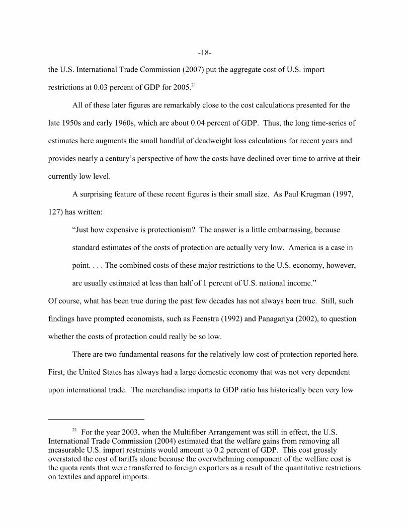
Figure 2 shows the annual deviation of the TRI-A from the average tariff measure.

Because the import-weighted average tariff does not include the variance of the tariff rates across

goods, the average tariff can understate the TRI by a significant margin. Over this period, TRI-A

exceeds the average tariff by about 75 percent, on average. Other calculations have found

deviations of similar magnitudes: Anderson and Neary (2005, 286) calculate that the TRI is

about 50 percent higher than the average tariff for the United States in 1990, and Kee, Nicita,

Olarreaga (2008, 679) found that the TRI is about 80 percent higher than the import-weighted

average tariff, on average, across many countries. In this case considered here, the largest

deviations are found during periods of significant tariff changes, such as the 1910s and the

1930s, when tariff rates were adjusted and import price movements were large. In addition, the

deviations are relatively small when the average tariff is high, but become more pronounced

when the average tariff is relatively low.

Figure 3 displays the different calculations of the TRI based on the four estimates of

elasticities from Table 1. The TRI estimates are very close in magnitude and only occasionally

deviate from one another by more than 5 percentage points. Once again, this is due to the fact

that the TRI depends almost entirely on the mean and the variance of tariff rates, rather than the

tariff-elasticity covariance. This figure reveals that the average tariff on imports and the all the

TRIs are highly correlated. The correlation coefficient of the average tariff and the calculated

TRI are 0.83 for TRI-B, and 0.88 for TRI-C, and 0.93 for TRI-D.

These findings give us some perspective on the longstanding concern that the average

tariff measure is significantly biased. As Rodríguez and Rodrik (2001, 316) noted:

-12-

Rodríguez and Rodrik conclude that “an examination of simple averages of taxes on17

imports and exports and NTB coverage ratios leaves us with the impression that these measuresin fact do a decent job of rank-ordering countries according to the restrictiveness of their traderegimes.”

“It is common to assert . . . that simple trade-weighted tariff averages or non-tariff

coverage ratios - which we believe to be the most direct indicators of trade restrictions -

are misleading as indicators of the stance of trade policy. Yet we know of no papers that

document the existence of serious biases in these direct indicators, much less establish

that an alternative indicator ‘performs’ better (in the relevant sense of calibrating the

restrictiveness of trade regimes).” 17

The results here suggest that the standard average tariff measure is highly correlated with a better

measure of trade restrictiveness, but that it understates it by a considerable margin. Therefore,

the conclusion of this exercise is that calculating something like a TRI is useful because the

average tariff ignores the variance in tariff rates across different goods.

3. The Annual Deadweight Loss from U.S. Tariffs

The reduced-form TRI in equation (2) also yields a linear approximation of the static

deadweight loss that is identical to the standard formula popularized by Johnson (1960). The

formula for the deadweight loss as a share of GDP is

(4) .

Kee, Nicita, and Olarreaga (2008) show that this formula can also be divided into the three

elements that define the TRI, namely, the tariff average, the tariff variance, and the tariff-

-13-

elasticity covariance:

(5) .

Unlike the TRI, the calculated deadweight loss is sensitive to the elasticities of import demand.

However, it is sensitive to the average elasticity, not the covariance between the tariffs and the

elasticities, which once again will be a small component of the calculation.

The standard static welfare estimates of the costs of protection have many well-known

limitations that are worth repeating. These estimates understate the deadweight losses by

ignoring the costs of rent-seeking (Krueger 1974), the dynamic gains from trade in terms of

productivity improvements (Pavcnik 2002), the benefits of product variety (Broda and Weinstein

2004), and the endogeneity of protection (Trefler 1993, Lee and Swagel 1997). On the other

hand, the estimates here do not account for any improvement in the terms of trade as a result of

import tariffs (Broda, Limão, Weinstein 2008). Still, with these caveats in mind, such welfare

calculations are still routinely made and it should be interesting to see how historical estimates of

these costs compare with more recent estimates.

A. Historical Calculations for the United States

Table 2 reports the deadweight loss calculation for selected years. Figure 4 plots the

annual deadweight loss from the tariff as a percent of GDP using the three components in

equation 5. Once again, the average tariff and the tariff variance dominate the deadweight loss

(DWL) calculation, and the contribution of the tariff-elasticity covariance is negligible. The

figure suggests that the DWL from tariffs was highest in the late nineteenth century, amounting

to about one percent of GDP in the late 1860s and early 1870s. By 1910, the DWL declined to

-14-

Of course, as noted earlier, after 1961, the deadweight loss from tariffs alone would be18

a misleading indicator of the costs of U.S. trade restrictions because of the increasing use ofexport restraints agreements, first in textiles and steel and later other goods.

about one half of one percent of GDP. By the end of World War II, the DWL had fallen to

almost negligible levels.

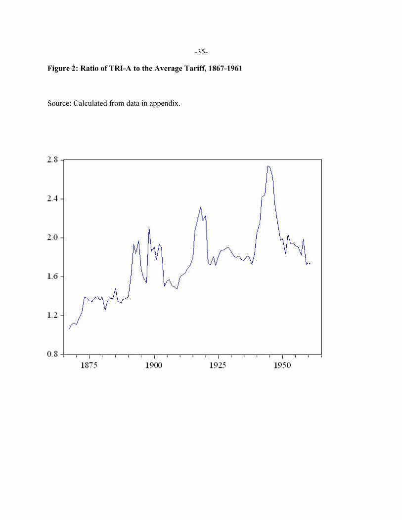
Although the TRI calculations are relatively insensitive to the particular elasticities used,

the deadweight loss estimates are much more sensitive to the average import-demand elasticity

used (rather than the tariff-elasticity covariance). Figure 5 shows the variation in the DWL

calculation depending upon the different elasticities used. These calculations are bounded by

DWLs that assume average elasticities of -1 and -3. Therefore, without solid information on the

elasticity of import demand, one cannot have a great deal of confidence in a precise figure that

accurately represents the DWL of the tariffs at any given moment. Instead, this figure indicates

that it is more appropriate to refer to a range within which the welfare loss falls. This range,

however, narrows with time. For example, the DWL after the Civil War were on the order of

roughly one percent of GDP. By the 1940s and 1950s, the range of DWL estimates had

narrowed significantly. Throughout most of this period, the United States did not employ many

non-tariff barriers on imports (such quantitative restrictions) so that these figures should

represent a reasonable confidence interval on the total static deadweight loss as a result of trade

barriers. 18

How does the time-series pattern of deadweight losses conform to our understanding of

the evolution of U.S. trade policy? It is not surprising that the highest costs of America’s tariff

policy came immediately after the Civil War, the heyday of America’s late nineteenth century

high-tariff policy. High and comprehensive duties on imports were imposed during the war and

remained in place for several years after the war in order to raise revenue for the federal

-15-

The welfare loss was much lower in 1859, when tariff rates were lower and much more19

uniform (only ad valorem duties were used from 1846 to 1860).

government. Only a tiny share of imports was allowed to enter the country without paying any19

duties. If the static welfare cost was about one percent of GDP, the associated redistribution of

income was much higher at about eight percent of GDP, according to estimates by Irwin (2007).

This large redistribution and associated deadweight loss may be one reason why the political

debate over trade policy was much more intense a century ago than today. By the mid-twentieth

century, the deadweight loss had fallen to about one-tenth of one percent of GDP, which not only

makes the historical figures of one percent of GDP seem much larger, but partly explains why,

after the early 1930s, trade policy was no longer a leading political issue in the country as it had

been in the late nineteenth century perhaps because the economic stakes were not as high.

The first major post-Civil War change in the tariff code occurred in 1873, when coffee,

tea, and other consumption items were put on the duty-free list. Because imports of these

commodities were quite large (coffee and tea alone accounted for 8 percent of U.S. imports in

1870), the share of U.S. imports that entered duty free rose from less than five percent prior to

1870 to nearly 30 percent. As a result, the deadweight cost of the tariff dropped significantly in

the early 1870s. The next significant change was the McKinley tariff of 1890, which temporarily

put sugar on the duty-free list, followed by the Wilson-Gorman Tariff of 1894. Both of these

acts helped push up the share of duty-free imports to about 50 percent of total imports and further

reduced the welfare losses from the tariff, although this was partially reversed by the Dingley

Tariff of 1897.

The TRI and deadweight losses fell further during the 1910s as a result of the drastically

reduced duties in the Underwood tariff of 1913 and a rise in the share of duty-free imports from

-16-

40 percent to 70 percent. Increased import duties in 1922 and 1930 (the Fordney-McCumber and

Hawley-Smoot tariffs, respectively) and import price deflation in the early 1930s produced a

higher TRI and somewhat larger deadweight losses in the interwar period. Given the attention to

trade protection in the interwar period, however, the increase in the deadweight loss is relatively

small in comparison to the late nineteenth century. Indeed, although the imposition of the

Smoot-Hawley tariff in 1930 and import price deflation helped increase the TRI from 26 percent

in 1929 to 35 percent in 1933, the DWL rises only slightly and generally remains around 0.23

percent of GDP. This figure is small primarily because dutiable imports as a share of GDP were

only 1.4 percent of GDP in 1929, prior to the tariff increases, while total imports (dutiable and

duty free) were just 4.1 percent of GDP. But the decline in the U.S. tariff due to higher import

prices and the liberalization brought about by the Reciprocal Trade Agreements Act of 1934

reversed this short-term trend (Irwin 1998a). By the late 1940s, the TRI and the deadweight

losses were at extremely low levels.

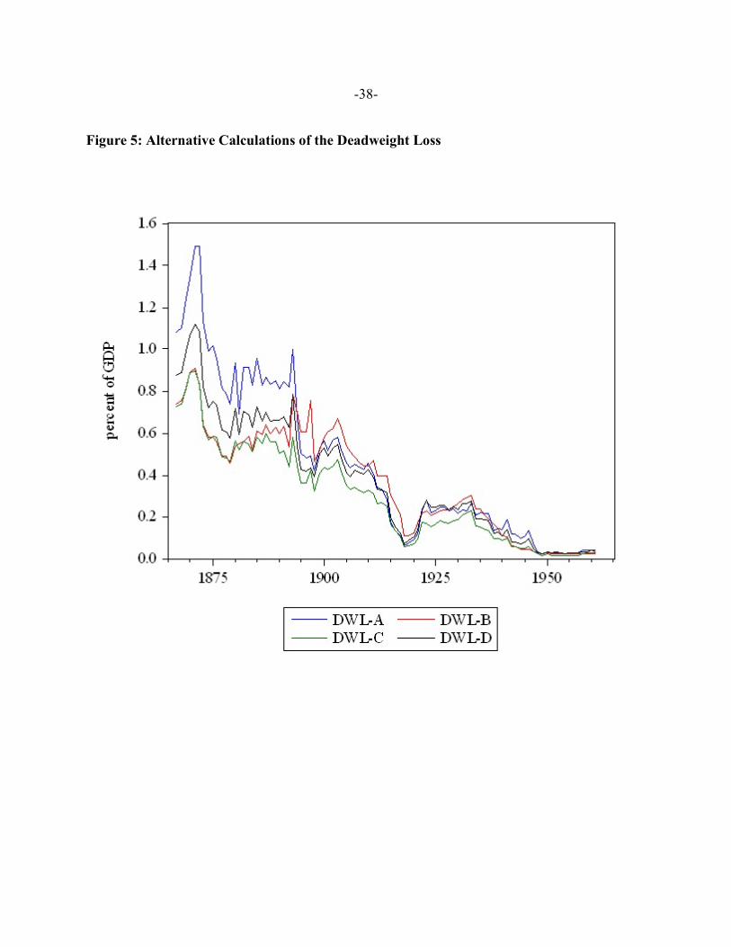
Thus, many of the big changes in the TRI and DWLs over time have been the result of

shifting large categories of imports on (and off) the duty-free list. Figure 6 shows several large

discrete jumps in the share of imports that receive duty-free treatment. This suggest that the TRI

and the average tariff on imports are not good measures of trade “protection” in the sense of

sheltering domestic producers from import competition. Many U.S. imports do not compete with

domestic production (such as coffee, tea, silk, tropical fruits, etc.) and are sometimes allowed to

enter without paying any duties, depending upon the revenue requirements of the government.

Thus, a substantial portion of imports may not subject to any trade limitations even as imports

that compete with domestic producers are severely restricted. Even if the overall TRI is low,

-17-

The McKinley tariff of 1890 illustrates the distinction between overall trade20

restrictions and trade protection. This tariff generally increased protective tariffs on dutiableimports, such as iron and steel and textiles, but the TRI and the deadweight loss fell substantiallyafter its enactment because it gave duty-free status to large swath of imports (Irwin 1998b). Theaverage tariff on dutiable imports might be a better broad indicator of trade protection in thesense of assisting import-competing producers.

imports of goods that affect domestic producers could still be burdened with heavy barriers. 20

B. Comparison to Recent Calculations

How do the historical DWL calculations compare with more recent estimates for the

United States? Kee, Nicita, and Olarreaga (2008) report the only TRI-based DWL calculation

for the United States for the early 2000s. They find that the import-weighted average tariff of

2.97 percent and the TRI-equivalent of 10.7 percent produces a deadweight loss of about $11

billion, or 0.09 percent of GDP (2004). This result is consistent with the present finding that by

the early 1960s the low level of U.S. tariffs had reduced the deadweight loss to less than one

tenth of one percent of GDP.

Other non-TRI-based estimates of the costs of protection for the U.S. economy, which are

also summarized on Table 2, also provide a comparison to the estimates here and bring them up-

to-date. Figure 7 compares the estimates presented in this paper with the scattered existing

calculations over recent years and illustrate how the figures for the 1950s and early 1960s

converge to the more recent estimates. Stern (1964) was the first person ever, to my knowledge,

to calculate the welfare cost of tariffs for the United States. For the year 1951, he found that the

cost was about 0.05 percent of GDP, virtually identical to the TRI-based estimate here of 0.04

percent of GDP. Estimates by Magee (1972) and Rousslang and Tokarick (1995) put the welfare

costs of U.S. tariffs in 1971 and 1987, respectively, at 0.04 percent of GDP. And most recently,

-18-

For the year 2003, when the Multifiber Arrangement was still in effect, the U.S.21

International Trade Commission (2004) estimated that the welfare gains from removing allmeasurable U.S. import restraints would amount to 0.2 percent of GDP. This cost grosslyoverstated the cost of tariffs alone because the overwhelming component of the welfare cost isthe quota rents that were transferred to foreign exporters as a result of the quantitative restrictionson textiles and apparel imports.

the U.S. International Trade Commission (2007) put the aggregate cost of U.S. import

restrictions at 0.03 percent of GDP for 2005. 21

All of these later figures are remarkably close to the cost calculations presented for the

late 1950s and early 1960s, which are about 0.04 percent of GDP. Thus, the long time-series of

estimates here augments the small handful of deadweight loss calculations for recent years and

provides nearly a century’s perspective of how the costs have declined over time to arrive at their

currently low level.

A surprising feature of these recent figures is their small size. As Paul Krugman (1997,

127) has written:

“Just how expensive is protectionism? The answer is a little embarrassing, because

standard estimates of the costs of protection are actually very low. America is a case in

point. . . . The combined costs of these major restrictions to the U.S. economy, however,

are usually estimated at less than half of 1 percent of U.S. national income.”

Of course, what has been true during the past few decades has not always been true. Still, such

findings have prompted economists, such as Feenstra (1992) and Panagariya (2002), to question

whether the costs of protection could really be so low.

There are two fundamental reasons for the relatively low cost of protection reported here.

First, the United States has always had a large domestic economy that was not very dependent

upon international trade. The merchandise imports to GDP ratio has historically been very low

-19-

De Melo and Tarr (1992) examined trade protection for the steel, automobiles, and22

textile industries in the mid-1980s and found that $14.7 billion of the $21.1 billion economic losswas due to quota rents, only $6.4 billion (0.16 percent of GDP) due to the domestic distortionarycost.

in comparison to other countries, at about 6 percent, even during the post World War II period

when import tariffs were low; only since the 1970s has the import share increased to its current

level of about 14 percent.

Second, for most of its history, the United States has not used highly distortionary trade

policy instruments, such as import quotas and import licenses, to block trade. Instead, it has

usually employed import tariffs, which - compared with alternatives - are a much more efficient

method of restricting trade. The problem with import quotas is that the foregone quota rents are

usually orders of magnitude larger than the tariff-induced distortions to resource allocation. For

example, the cost of U.S. trade restrictions was much higher in the 1970s and 1980s than decades

before or after because quantitative restrictions and voluntary export restraints were used to limit

imports of automobiles, textiles and apparel, iron and steel, semiconductors, and other products

(de Melo and Tarr 1992, Feenstra 1992). From 2002 to 2005, the International Trade22

Commission’s estimate of the cost of U.S. import barriers fell from $14.1 billion to $3.7 billion

almost entirely as a result of the expiration of the Multifiber Arrangement (MFA). The MFA

restricted developing country exports of textiles and apparel goods and generated large quota-

rents that were eliminated when the MFA expired.

Finally, it should be emphasized that the low costs of protection do not imply that the

gains from trade are small; indeed, the gains from trade could be enormous. Rather, these results

simply suggests that, in general, formal U.S. trade barriers have been at a very low level in recent

decades.

-20-

See Arce and Reinert (1994).23

C. Aggregation Bias

The calculations presented above indicate that the mean and variance of tariffs are the

most important contributing factors to the TRI and DWL. The precise results have been based

on the disaggregation of imports into 16 to 18 categories in the tariff schedule. However, as one

further disaggregates the tariff code, the variance of tariffs could increase. As a check on the23

extent to which the degree of aggregation matters for the calculated TRI and DWLs, the most

highly disaggregated import data available was used in calculations for selected years (1880,

1900, 1928, and 1938). These results are reported on Table 3. Rather than assign particular

elasticity values of the thousands of items in the import data, a uniform elasticity of -2 has been

assumed in each case reported in Table 3 to ensure comparability. When the elasticities of

import demand are assumed to be uniform across import categories, the tariff-elasticity

covariance is implicitly set to zero, in which case the particular elasticity chosen does not affect

the calculation of the TRI. As noted earlier, the tariff-elasticity covariance is only a tiny

component of the TRI and for much of the early sample the covariance is negative, meaning that

assuming a zero covariance between the elasticities and the import tariffs slightly overstates the

TRI in earlier samples and slightly understates it in later samples.

The results show that disaggregation – essentially adding more variance to the tariff

structure – matters a great deal for the TRI and DWL, up to a point. Moving from the simple

average tariff to about 16 import categories increases the TRI and the DWL by almost a factor of

two in each case. However, moving from 16 categories to more than 2,000 categories increases

the TRIs and DWLs somewhat more, but not much more. This seems to imply limited gains

from further disaggregation, at least in these cases.

-21-

Rousslang (1987) compares the revenue costs of U.S. tariffs in the 1980s with other24

taxes.

D. Average Welfare Cost per Dollar of Revenue

From 1867 until the introduction of the income tax in 1913, import duties raised about

half of the revenue received by the federal government. The important role of the tariff in public

finance raises the question of its efficiency as a revenue-raising tax. Figure 8 presents the

average DWL incurred from import duties per dollar revenue raised by those duties. The average

welfare cost per dollar of revenue for this period is 46 cents for 1867-1913 and 40 cents for

1867-1961. The spike in the figure around 1890 is due to the McKinley tariff of that year, which

reduced the tax base (dutiable imports) and raised tax rates. Behind these average figures is a

great deal of variance in the average welfare cost across different sections of the tariff schedule.

Imports that were taxed a low or moderate rates (metals, leather) had welfare costs of about 20 to

30 cents per dollar revenue, while highly taxed imports (silk, spirits) had welfare costs of 80

cents or more per dollar revenue. However, it appears that the pre-Civil War tariff code (1859)

was highly efficient in having a welfare cost per dollar of revenue of just about 20 cents.

While there does not appear to be any historical estimates of the excess burden associated

with taxes a century ago, this figure can be compared - with caution - to contemporary estimates

of the marginal welfare cost of taxation. There are many estimates of the marginal excess24

burden per additional dollar of tax revenue in the public finance literature, but those of Ballard,

Shoven, and Whalley (1985) have been widely cited in the case of the United States. Their

central estimate is 33 cents per dollar of revenue, but the estimates range from 17 cents to 56

cents, depending upon the elasticity of labor supply and the savings elasticity. In their central

-22-

case, the marginal excess burden is 46 cents for capital taxes, 23 cents for labor taxes, 31 cents

for income taxes, and 39 cents for consumer sales taxes. While the average welfare cost per

dollar revenue a century ago is roughly comparable to the marginal welfare cost more recently,

any direct comparison is problematic. In particular, the average cost of tariffs is likely to be

significantly lower than the marginal cost of those tariffs, invalidating the comparison. Still,

although in principle a consumption or sales tax should raise more revenue with less distortion

than a tariff, import duties were probably much easier to collect and enforce in the late nineteenth

century than other modes of taxation.

4. Conclusions

This paper presents a simplified trade restrictiveness index for the United States during a

long period in its history when import tariffs were the only major policy impediment to

international trade and formal non-tariff barriers (such as import quotas) were not prevalent. The

results show that the commonly used import-weighted average tariff is highly correlated with the

Anderson-Neary (2005) trade restrictiveness index, although it understates the index by about 75

percent, on average.

More importantly, the paper presents annual estimates of static deadweight loss from the

U.S. tariff code for nearly a century. These annual estimates provide a sharp contrast for the

isolated handful of estimates for individual years in the post-World War II period. Unlike the

low deadweight loss estimates in recent decades, the results here indicate that the losses were

quite large in the years immediately after the Civil War, at about one percent of GDP. Since

then, they have declined secularly to less than one tenth of one percent of GDP by the end of

World War II. This decline in the welfare cost of tariffs is due to the rising share of imports that

-23-

were given duty free access to the U.S. market and the decline in rates of import duty.

Historically, the cost of protection has been low for the United States because international trade

has been a relatively small part of the overall economy and import tariffs are much less

distortionary than other trade interventions, such as import quotas or import licences. In

addition, import duties seems to have been a relatively efficient means of raising revenue: the

average welfare cost per dollar revenue raised was about 40 cents during the period considered in

this paper, somewhat higher than current estimates for the modern tax system.

-24-

References

Anderson, James E., and J. Peter Neary. 2005. Measuring the Restrictiveness of InternationalTrade Policy. Cambridge: MIT Press.

Arce, Hugh M., and Kenneth A. Reinert. 1994. “Aggregation and the Welfare Analysis of U.S.Tariffs.” Journal of Economic Studies 21, 26-30.

Ballard, Charles L., John B. Shoven, and John Whalley. 1985. “General EquilibriumComputations of the Marginal Welfare Costs of Taxes in the United States.” American EconomicReview 75, 128-138.

Broda, Christian, and David Weinstein. 2004. “Globalization and the Gains from Variety.”Quarterly Journal of Economics 121, 541-586.

Broda, Christian, Nuno Limão, and David Weinstein. 2008. “Optimal Tariffs and Market Power:The Evidence.” American Economic Review, forthcoming.

Dakhlia, Sami, and Akram Temimi. 2006. “An Extension of the Trade Restrictiveness Index toLarge Economies,” Review of International Economics. 14, 678-682.

De Melo, Jaime, and David Tarr. 1992. A General Equilibrium Analysis of U.S. Foreign TradePolicy. Cambridge: MIT Press.

Estevadeordal, Antoni. 1997. “Measuring Protection in the Early Twentieth Century.” European Review of Economic History 1, 89-125.

Feenstra, Robert C. 1992. “How Costly Is Protectionism?” Journal of Economic Perspectives 6,159-178.

Feenstra, Robert C. 1995. “Estimating the Effects of Trade Policy.” In Handbook ofInternational Economics, Vol. 3, edited by Gene Grossman and Kenneth Rogoff. Amsterdam: Elsevier.

Ho, Mun S., and Dale W. Jorgenson. 1994. “Trade Policy and U.S. Economic Growth,” Journalof Policy Modeling 16, 119-146.

Irwin, Douglas A. 1998a. “Changes in U.S. Tariffs: The Role of Import Prices and CommercialPolicies.” American Economic Review, 88, 1015-1026.

Irwin, Douglas A. 1998b. “Higher Tariffs, Lower Revenues? Analyzing the Fiscal Aspects ofthe ‘Great Tariff Debate of 1888.’” Journal of Economic History 58, 59-72.

Irwin, Douglas A. 2007. “Tariff Incidence in America’s Gilded Age.” Journal of EconomicHistory 67, 582-607.

-25-

Johnson, Harry. 1960. “The Cost of Protection and the Scientific Tariff.” Journal of PoliticalEconomy 68, 327-345.

Johnston, Louis D. and Samuel H. Williamson. 2006. “The Annual Real and Nominal GDP forthe United States, 1790 - Present.” Economic History Services, April 1. URL :http://eh.net/hmit/gdp/

Kee, Hiau L., Alessandro Nicita, and Marcelo Olarreaga. 2008. “Import Demand Elasticitiesand Trade Distortions.” Review of Economics and Statistics, 90, 666-682.

Kee, Hiau L., Alessandro Nicita, and Marcelo Olarreaga. 2009. “Estimating TradeRestrictiveness Indices,” Economic Journal 119, 172-199.

Kreinin, Mordechai. 1973. “Disaggregated Import Demand Functions: Further Results.” Southern Economic Journal 40, 19-25.

Krueger, Anne O. 1974. “The Political Economy of a Rent Seeking Society.” AmericanEconomic Review 64, 291-303.

Krugman, Paul. 1997. Age of Diminished Expectations, 3 edition. Cambridge: MIT Press.rd

Leamer, Edward E. 1974. “Nominal Tariff Averages with Estimated Weights.” SouthernEconomic Journal 41, 34-46.

Lerdau, E. 1957. “On the Measurement of Tariffs: The U.S. Over Forty Years.” EconomiaInternazionale 10, 232-244.

Lee, Jong-Wha, and Phillip Swagel. 1997. “Trade Barriers and Trade Flows across Countriesand Industries.” Review of Economics and Statistics, 79, 372-82.

Loveday, Alexander. 1929. “The Measurement of Tariff Levels.” Journal of the RoyalStatistical Society 92, 487-529.

Magee, Stephen P. 1972. “The Welfare Effects of Restrictions on U.S. Trade.” Brookings Paperson Economic Activity, 3, 645-701.

Marquez, Jaime. 1994. “The Econometrics of Elasticities or the Elasticity of Econometrics: AnEmpirical Analysis of the Behavior of U.S. Imports.” Review of Economics and Statistics 76,471-481.

Marquez, Jaime. 1999. “Long-Period Trade Elasticities for Canada, Japan, and the UnitedStates.” Review of International Economics 7, 102- 116.

O’Rourke, Kevin. 1997. “Measuring Protection: A Cautionary Tale.” Journal of DevelopmentEconomics 53, 169-83.

-26-

Panagariya, Arvind. 2002. “Cost of Protection: Where Do We Stand?” American EconomicReview 92, 175-179.

Pavcnik, Nina. 2002. “Trade Liberalization, Exit, and Productivity Improvements: Evidencefrom Chilean Plants.” Review of Economic Studies 69, 245-76.

Rodríguez, Francisco, and Dani Rodrik. 2001. “Trade Policy and Economic Growth: ASkeptic’s Guide to the Cross-National Evidence.” In NBER Macroeconomics Annual 2000,edited by Ben Bernanke and Kenneth S. Rogoff. Cambridge: MIT Press.

Rousslang, Donald. 1987. “The Opportunity Cost of Import Tariffs.” Kyklos 40, 88-103.

Rousslang, Donald J., and Stephen P. Tokarick. 1995. “Estimating the Welfare Cost of Tariffs:The Roles of Leisure and Domestic Taxes.” Oxford Economic Papers 47, 83-97.

Shiells, Clinton R., Robert M. Stern, and Alan V. Deardorff. 1986. “Estimates of the Elasticitiesof Substitution between Imports and Home Goods for the United States.” WeltwirtschaftlichesArchiv 122, 497-519.

Stern, Robert M. 1964. “The U.S. Tariff and the Efficiency of the U.S. Economy.” AmericanEconomic Review 54, 459-470.

Stern, Robert M., Jonathan Francis, and Bruce Schumacher. 1976. Price Elasticities inInternational Trade: An Annotated Bibliography, London: Macmillan.

Trefler, Daniel. 1993. “Trade Liberalization and the Theory of Endogenous Protection: AnEconometric Study of U.S. Import Policy.” Journal of Political Economy 101, 138-60.

U.S. Bureau of the Census. 1975. Historical Statistics of the United States, BicentennialEdition. Washington, D.C.: Government Printing Office.

U.S. Department of the Treasury. 1923. Annual Report, Washington, D.C.: GPO.

U.S. International Trade Commission. 2004. Economic Effects of Significant U.S. ImportRestraints, Publication 3701, Fourth Update, June.

U.S. International Trade Commission. 2007. Economic Effects of Significant U.S. ImportRestraints, Publication 3906, Fifth Update, February.

U.S. Senate. 1894. “Imports and Exports. Part I. Imports from 1867 to 1893, inclusive.” SenateReport No. 259, Part 1, 53 Congress, 2 Session, Congressional Serial Set vol. 3182.rd nd

-27-

Data Appendix

Year Imports ofmerchandise for

consumption

Nominal GDP

Imports/GDP

Import-weighted

average tariff

TRI (A) DWL/GDP

(millions $) (billions $) (percent) (percent) (percent) (percent)

1859 317 4.38 7.2 15.4 17.9 -0.22

1867 378 8.33 4.5 44.6 47.0 -0.85

1868 345 8.14 4.2 46.6 49.0 -0.84

1869 394 7.85 5.0 44.8 47.6 -0.96

1870 426 7.79 5.5 44.9 47.7 -1.04

1871 500 7.68 6.5 40.5 44.6 -1.10

1872 560 8.21 6.8 38.0 43.0 -1.06

1873 663 8.68 7.6 27.9 35.6 -0.80

1874 568 8.43 6.7 28.3 35.4 -0.70

1875 526 8.05 6.5 29.4 36.2 -0.72

1876 465 8.21 5.7 31.3 38.6 -0.70

1877 440 8.27 5.3 29.2 37.0 -0.61

1878 439 8.31 5.3 29.0 37.0 -0.58

1879 440 9.36 4.7 30.3 38.1 -0.56

1880 628 10.40 6.0 29.1 37.3 -0.70

1881 651 11.60 5.6 29.8 37.4 -0.67

1882 717 12.20 5.9 30.2 37.8 -0.71

1883 701 12.30 5.7 30.0 37.7 -0.68

1884 668 11.80 5.7 28.5 35.8 -0.61

1885 579 11.40 5.1 30.8 41.3 -0.75

1886 624 12.00 5.2 30.4 37.1 -0.60

1887 680 13.00 5.2 31.5 38.0 -0.64

1888 707 13.80 5.1 30.6 37.4 -0.61

1889 735 13.80 5.3 30.0 36.9 -0.61

1890 766 15.20 5.0 29.6 40.9 -0.81

1891 845 15.50 5.5 25.7 40.4 -0.84

1892 804 16.40 4.9 21.7 41.5 -0.82

1893 833 15.50 5.4 23.9 43.7 -1.00

1894 630 14.20 4.4 20.6 40.3 -0.67

1895 731 15.60 4.7 20.4 34.0 -0.51

1896 760 15.40 4.9 20.7 32.5 -0.48

1897 789 16.10 4.9 21.9 33.4 -0.49

1898 587 18.20 3.2 24.8 38.2 -0.42

1899 685 19.50 3.5 29.5 41.6 -0.53

1900 831 20.70 4.0 27.6 38.3 -0.56

1901 808 22.40 3.6 28.9 39.5 -0.61

1902 900 24.20 3.7 28.0 41.4 -0.64

1903 1008 26.10 3.9 27.9 42.0 -0.68

1904 982 25.80 3.8 26.3 39.3 -0.52

-28-

1905 1087 28.90 3.8 23.8 37.0 -0.46

1906 1213 30.90 3.9 24.2 36.4 -0.43

1907 1415 34.00 4.2 23.3 35.0 -0.45

1908 1183 30.30 3.9 23.9 35.7 -0.43

1909 1282 32.20 4.0 23.0 36.4 -0.43

1910 1547 33.40 4.6 21.1 33.8 -0.46

1911 1528 34.30 4.5 20.3 32.6 -0.40

1912 1641 37.40 4.4 18.6 30.4 -0.34

1913 1767 39.10 4.5 17.7 29.6 -0.33

1914 1906 36.50 5.2 14.9 25.4 -0.29

1915 1648 38.70 4.3 12.5 22.3 -0.18

1916 2359 49.60 4.8 9.1 18.8 -0.13

1917 2919 59.70 4.9 7.0 16.4 -0.11

1918 2952 75.80 3.9 5.8 14.0 -0.06

1919 3828 78.30 4.9 6.2 13.5 -0.07

1920 5102 88.40 5.8 6.4 14.2 -0.09

1921 2557 73.60 3.5 11.4 19.8 -0.11

1922 3074 73.40 4.2 14.7 25.3 -0.23

1923 3732 85.40 4.4 15.2 27.4 -0.28

1924 3575 87.00 4.1 14.9 25.5 -0.22

1925 4176 90.60 4.6 13.2 24.0 -0.23

1926 4408 97.00 4.5 13.4 25.1 -0.24

1927 4163 95.50 4.4 13.8 25.8 -0.25

1928 4078 97.40 4.2 13.3 25.2 -0.23

1929 4339 103.60 4.2 13.5 25.7 -0.24

1930 3114 91.20 3.4 14.8 27.1 -0.21

1931 2088 76.50 2.7 17.8 32.0 -0.24

1932 1325 58.70 2.3 19.6 34.8 -0.23

1933 1433 56.40 2.5 19.8 35.3 -0.26

1934 1636 66.00 2.5 18.4 32.2 -0.21

1935 2039 73.30 2.8 17.5 31.2 -0.22

1936 2424 83.80 2.9 16.8 30.2 -0.22

1937 3010 91.90 3.3 15.6 27.9 -0.21

1938 1950 86.10 2.3 15.5 26.8 -0.13

1939 2276 92.20 2.5 14.4 26.5 -0.14

1940 2541 101.40 2.5 12.5 25.6 -0.14

1941 3222 126.70 2.5 13.6 29.5 -0.19

1942 2780 161.90 1.7 11.5 27.8 -0.11

1943 3390 198.60 1.7 11.6 28.2 -0.12

1944 3887 219.80 1.8 9.5 25.8 -0.10

1945 4098 223.10 1.8 9.3 26.2 -0.11

1946 4825 222.30 2.2 9.9 26.5 -0.13

1947 5666 244.20 2.3 7.6 17.8 -0.06

1948 7092 269.20 2.6 5.7 12.3 -0.03

1949 6592 267.30 2.5 5.5 10.7 -0.02

1950 8743 293.80 3.0 6.0 11.9 -0.04

1951 10817 339.30 3.2 5.5 10.0 -0.03

-29-

1952 10747 358.30 3.0 5.3 10.8 -0.03

1953 10779 379.40 2.8 5.4 10.6 -0.03

1954 10240 380.40 2.7 5.2 10.1 -0.02

1955 11337 414.80 2.7 5.6 10.8 -0.03

1956 12516 437.50 2.9 5.7 10.9 -0.03

1957 12951 461.10 2.8 5.8 10.6 -0.03

1958 12739 467.20 2.7 6.4 12.9 -0.04

1959 14994 506.60 3.0 7.0 12.1 -0.04

1960 14650 526.40 2.8 7.4 12.9 -0.04

1961 14658 544.70 2.7 7.2 12.5 -0.04

Sources: Imports for consumption: U.S. Bureau of the Census (1975), series U-207. NominalGDP: Johnston and Williamson (2006). Import-weighted average tariff: U.S. Bureau of theCensus (1975), series U-211.

Note: The elasticity values reported in Table 1-A are used in the calculation of the TRI and theDWL.

-30-

Table 1: Average U.S. Import Duties (percent) and Import Demand Elasticities, by Tariff Schedule, selected years

1867 1890 1925 1950 Elasticities of Import Demand

A B C D

Schedule A Chemicals, oils, paints 34.6 32.0 29.3 15.5 -2.53 -7.18 -1.1 -0.97

Schedule B Earthenware and glassware 45.8 57.2 43.5 26.5 -2.85 -2.12 -1.72 -1.37

Schedule C Metals and manufactures 27.2 35.4 34.3 13.0 -1.68 -1.51 -1.5 -2.0

Schedule D Wood and manufactures 21.8 16.1 22.4 3.6 -1.40 -5.44 -1.36 -0.96

Schedule E Sugar, molasses, &manufactures

68.7 63.0 62.8 10.5 -0.66 -0.66 -1 -1.0

Schedule F Tobacco & manufactures 130.6 80.1 50.7 24.8 -1.13 -7.57 -2.59 -1.13

Schedule G Agricultural products 26.9 25.6 23.3 10.7 -1.13 -0.21 -0.62 -1.13

Schedule H Spirits, wines, & beverages 119.5 68.5 42.4 25.1 -1.64 -0.70 -1 -1.0

Schedule I Cotton manufactures 40.1 39.9 30.7 23.8 -3.94 -1.41 -1.35 -2.43

Schedule J Flax, hemp, jute, &manufactures

35.1 25.3 17.9 6.4 -1.14 -1.41 -1.35 -2.43

Schedule K Wool & manufactures 50.7 61.0 43.7 23.9 -3.92 -0.52 -1.35 -2.43

Schedule L Silk & silk goods 58.6 49.5 53.1 30.6 -3.92 -0.52 -1.35 -2.43

Schedule M Pulp, paper, & books 30.7 19.3 23.6 9.9 -0.69 -1.63 -1.2 -1.44

Schedule N Sundries 32.4 24.7 38.3 18.2 -1.66 -1.66 -1.14 -4.44

Source: for years 1867 to 1889: U.S. Senate (1894), for years 1890 to 1961, annual report of the U.S. Department of Treasury and Statistical Abstract of theUnited States. Elasticities of import demand are from (A) Stern, Francis, and Schumacher (1976), table 2.3, p. 22; (B) Shiells, Stern, and Deardorff (1986),Table 4, p. 515; (C) Ho and Jorgenson (1994), Table 1; (D) Kreinin (1973),

-31-

Table 2: Average Tariffs, Trade Restrictiveness Indices, and Welfare Losses, selected years

Average Tariffon TotalImports

AverageTariff onDutiableImports

Coefficientof Variation

of TariffRates

Share ofImports Duty

Free

MerchandiseImports/GDP

Ratio

TRI (A) DWL(millions)

DWL/GDP(percent)

1859 15.4 19.6 0.38 21.1 7.2 17.9 $9.4 0.22

1867 44.6 46.7 0.65 4.5 4.5 47.0 $71 0.85

1875 29.4 40.7 0.53 27.8 6.5 36.2 $58 0.72

1885 30.8 46.1 0.57 33.2 5.1 41.2 $86 0.75

1890 29.6 44.6 0.55 33.7 5.0 40.9 $123 0.81

1900 27.6 49.5 0.55 44.2 4.0 38.3 $116 0.56

1910 21.1 41.6 0.55 49.2 4.6 33.8 $153 0.46

1922 14.7 38.1 0.52 61.4 4.2 25.2 $167 0.23

1929 13.5 40.1 0.54 66.4 4.2 25.7 $244 0.24

1931 17.8 53.2 0.63 66.7 2.7 32.0 $180 0.24

1938 15.5 37.8 0.48 60.7 2.3 26.8 $115 0.13

1946 10.3 25.3 0.70 61.0 2.2 26.5 $292 0.13

1950 6.1 13.1 0.58 54.5 3.0 11.9 $105 0.04

1960 7.2 12.2 0.61 39.5 2.8 12.9 $208 0.04

-32-

Other TRI Estimates for the United States

Average Tariffon Total Imports

Average Tariffon Dutiable

Imports

Share of ImportsDuty Free

Imports/GDP TRI DWL(millions)

DWL/GDP(percent)

1990 4.0 5.0 32.8 8.5 6.1 NA NA

2004 3.0 4.8 69.6 12.5 10.7 $11,060 0.09

1990: Anderson and Neary (2005, 286), general equilibrium, assumed elasticities of substitution, 1200 import categories, two composite final goods, no quotas.2004: Kee, Nicita, and Olarreaga (2008), partial equilibrium, estimated import demand elasticities, 4625 tariff lines, does not include import quotas

Other Estimates for the United States

Average Tariffon Total Imports

Average Tariffon Dutiable

Imports

Share of ImportsDuty Free

Imports/GDP TRI DWL(millions)

DWL/GDP(percent)

1951 5.5 12.5 55.4 3.2 NA $183 0.05

1971 6.1 9.2 33.6 4.0 NA $493 0.04

1985 3.8 5.5 30.9 8.1 23.7 NA NA

1987 3.5 5.2 32.9 8.5 NA $1, 900-3,000 0.04-0.06

2005 1.4 4.6 69.6 13.5 NA $3,700 0.03

1951: Stern (1964, 465), partial equilibrium, tariffs only, no terms of trade effects, does not include import quotas1971: Magee (1972, 666), partial equilibrium, tariffs only, no terms of trade effects, does not include import quotas1985: de Melo and Tarr (1992, 200), general equilibrium, uniform tariff yielding same welfare distortionary cost as existing import quotas (excluding rents)1987: Rousslang and Tokarick (1995), general equilibrium, tariffs only, no terms of trade effects, does not include import quotas2005: U.S. International Trade Commission (2007), general equilibrium, dynamic, no terms of trade effect

-33-

Table 3: Effects of Aggregation on TRIs and DWLs, selected years

Assumption: elasticity of import demand = -2.0

Year Number of Import Lines TRI(percent)

DWL/GDP(percent)

1880 1 29.1 -0.5

17 37.3 -0.8

1,290 44.2 -1.2

1900 1 27.5 -0.3

16 39.4 -0.6

2,390 42.7 -0.8

1928 1 13.3 -0.1

15 24.6 -0.3

5,505 32.5 -0.4

1932 1 19.4 -0.1

16 40.8 -0.4

5,248 43.8 -0.5

1938 1 15.5 -0.1

17 25.0 -0.2

2,882 33.8 -0.2

Source: Disaggregated import and tariff data is available in the Foreign Commerce and Navigationyearbooks published by the Department of Commerce.

-34-

Figure 1: Average U.S. Tariff on Imports and Trade Restrictiveness Index, 1867-1961

-35-

Figure 2: Ratio of TRI-A to the Average Tariff, 1867-1961

Source: Calculated from data in appendix.

-36-

Figure 3: Alternative Calculations of the TRI

-37-

Figure 4: Deadweight Loss from U.S. Import Tariffs, 1867-1961

-38-

Figure 5: Alternative Calculations of the Deadweight Loss

-39-

Figure 6: Share of Duty-Free Imports in Total Imports, 1867-1961

Source: U.S. Bureau of the Census (1975), series U-207, 208

-40-

Figure 7: Comparison of Deadweight Loss Estimates from U.S. Import Tariffs

Note: From TRI (A) and other estimate on Table 2. The ITC estimate for 2002 includes importquotas (notably the Multifiber Arrangement); the ITC estimate for 2005 occurs after the MFAexpires.

-41-

Figure 8: U.S. Tariffs – Average Welfare Cost per Dollar Revenue