Embed Size (px)
Citation preview

This paper uses a rich dataset of financial and macroeconomic variables for euro area economies, and a range of econometric techniques, to discuss challenges in predicting episodes of market access tensions by sovereign borrowers.
DisclaimerThis working paper should not be reported as representing the views of the ESM. The views expressed in this Working Paper are those of the authors and do not necessarily represent those of the ESM or ESM policy.
Working Paper Series | 42 | 2020
Quantifying risks to sovereign market access: Methods and challenges
Diana Zigraiova European Stability Mechanism, Charles University
Aitor Erce European Investment Bank, European University Institute
Xu JiangEuropean Stability Mechanism

DisclaimerThis Working Paper should not be reported as representing the views of the ESM. The views expressed in this Working Paper are those of the authors and do not necessarily represent those of the ESM or ESM policy. No responsibility or liability is accepted by the ESM in relation to the accuracy or completeness of the information, including any data sets, presented in this Working Paper.
© European Stability Mechanism, 2020 All rights reserved. Any reproduction, publication and reprint in the form of a different publication, whether printed or produced electronically, in whole or in part, is permitted only with the explicit written authorisation of the European Stability Mechanism.
Quantifying risks to sovereign marketaccess: Methods and challengesDiana Zigraiova 1 European Stability Mechanism
Aitor Erce 2 European Investment Bank, European University Institute
Xu Jiang 3 European Stability Mechanism
1 [email protected] [email protected] [email protected]
AbstractIn this paper we use data from the euro area to study episodes when sovereigns lose market access. We construct a detailed dataset with potential indicators of market access tensions, and evaluate their ability to forecast episodes when market access is lost, using various econometric approaches. We find that factors associated with high market access tensions are not limited to financial markets, but also encompass developments in global demand, macroeconomic conditions and the fiscal stance. Using the top-performing indicators, we construct a number of market tension indices and use them as single predictors of market access tensions. While such indices are helpful in capturing worsening conditions, they do not yield satisfactory out-of-sample results. On the other hand, using the same top-performing indicators in various multivariate models generates good forecasts of upcoming difficulties in accessing sovereign bond markets. Our results thus point to a trade-off between communicability and accuracy that policymakers face in the search for tools to evaluate risks to market access.
Working Paper Series | 42 | 2020
Keywords: Euro area sovereign bond market; forecasting; sovereign debt crises, sovereign market access; variable selection
JEL codes: C53, G01, G15
ISSN 2443-5503 ISBN 978-92-95085-83-1
doi:10.2852/207770EU catalog number DW-AB-20-001-EN-N
1
Quantifying risks to sovereign market access:
Methods and challenges
Diana Zigraiova Aitor Erce Xu Jiang
January 2020
Abstract: In this paper we use data from the euro area to study episodes when sovereigns lose market access. We construct a detailed dataset with potential indicators of market access tensions, and evaluate their ability to forecast episodes when market access is lost, using various econometric approaches. We find that factors associated with high market access tensions are not limited to financial markets, but also encompass developments in global demand, macroeconomic conditions and the fiscal stance. Using the top-performing indicators, we construct a number of market tension indices and use them as single predictors of market access tensions. While such indices are helpful in capturing worsening conditions, they do not yield satisfactory out-of-sample results. On the other hand, using the same top-performing indicators in various multivariate models generates good forecasts of upcoming difficulties in accessing sovereign bond markets. Our results thus point to a trade-off between communicability and accuracy that policymakers face in the search for tools to evaluate risks to market access.
Introduction
The lack of a central bank explicitly playing the role of lender-of-last-resort for governments, combined
with the magnitude of public debt stocks, had two negative consequences that exacerbated the euro
area crisis. First, markets for government bonds lacked a stabilizing tool against the ongoing liquidity
runs, and this triggered a recessionary tightening of financing conditions. Second, domestic banks were
induced to become lenders of last resort, setting the stage for destabilising doom-loops that reinforced
the effect of the worsening financing conditions. Such extreme tensions in deep and highly liquid public
bond markets caught most by surprise (Casalinho et al. 2016).1
While the theoretical literature is large, there is just a handful of papers that have focused on
understanding empirically what drives tensions in euro area public bond markets. A consequence of
this is that, as recently acknowledged by the International Monetary Fund in its 2018 Review of
Conditionality (ROC, 2018), existing policy tools for detecting sovereign debt crises and risks to market
We thank Jaroslav Baran, Anastasia Guscina, Carlos Martins, Jacques Netzer, Stephanie Pamies, Markus Rodlauer, Rolf Strauch, Sheetal Tewari and seminar participants at the IMF workshop on "Fiscal Policies in a Challenging World" and the
European Stability Mechanism for their suggestions. We are grateful to the European Stability Mechanism’s Investment and Funding teams, who provided us with two separate detailed lists of market indicators to be tracked. Diana is with the European
Stability Mechanism and Institute of Economic Studies at Charles University. Xu is with the European Stability Mechanism. Aitor is with the European Investment Bank and the European University Institute. Disclaimer: This paper does not develop an
operational methodology for determining market access for evaluating eligibility for precautionary financing by the European Stability Mechanism. All the views presented in this paper are the authors’ and not those of the institutions the authors are
affiliated with. Corresponding author: Diana Zigraiova, [email protected] 1 The ample literature studying public debt auctions in advanced economies does not consider LMA episodes (Sigaux 2018 or
Belton et al. 2018). Sovereign loss of market access has traditionally been focused on emerging countries (Gelos et al. 2004).

2
access were designed for countries with critically different public debt markets than those in more
advanced economies – where markets are deeper, more liquid, and debt is mostly denominated in the
local currency. In fact, while Greece has become the poster child for the potentially devastating effects
of losing the confidence of market creditors, there is still a lack of analytical understanding on how to
predict an episode of a sovereign losing access to its domestic bond market.2 This paper contributes to
filling this analytical gap.
De Broeck & Guscina (2011) study the effect of the global crisis on issuance strategies of advanced
economy sovereigns. They document a deviation away from plain-vanilla bond issuance, especially in
countries with high deficits and high debt levels. Bassanetti, Cottarelli & Presbitero (2016) study the
role of debt flows for understanding market access. Fisher (2012) discusses the importance of
understanding the drivers of demand for public debt. Casalinho et al. (2016) review the experience of
Ireland, Portugal, Cyprus and Spain in re-accessing the market after their official programs ended.
Schalck (2017) estimates reaction functions to identify shifts in the behaviour of public debt managers,
and shows that, following the crisis, France’s funding strategy shifted towards cost minimisation.
Guscina, Malik & Papaioannou (2017) provide an operational definition of loss of market access (LMA)
and examine the predictive capacity of potential leading indicators of LMA.3 One lesson from the
literature and from our discussions with bond traders is that market access depends on a host of factors
and, depending on the information available, can be assessed in a variety of ways.
In this paper we contribute to this literature in at least two fronts. First, using a selected set of indicators
chosen by two teams of financial market participants (experts on primary and secondary markets) and
a thorough reading of the academic literature, we construct an extensive and detailed dataset of
potential leading indicators of market access tensions. Second, we evaluate these selected indicators
systematically, using a variety of univariate and multivariate econometric frameworks. We use
univariate analysis to select the best indicators from our rich dataset. While forward rate difference
from the best performer emerged as the most important predictor of market access tensions, we find
that factors associated with high market access tensions are not limited to financial markets, but also
encompass developments in global demand, macroeconomic factors and the fiscal stance.
We propose an easy-to-construct and transparent index summarising the set of best indicators of
market access tensions, and use it to understand the driving forces of past episodes of market access
tensions. We also use a variety of econometric methods to predict future tensions to market access.
We show that multivariate methods perform better than the univariate index. We also show that
models allowing for endogenous selection of explanatory variables perform better in terms of detecting
increased market access tensions, although that may come at the cost of more false alarms.
The rest of this paper is organized as follows: Section 2 provides our definition of episodes when
sovereigns lose market access. Section 3 lists those primary market, secondary market and demand and
supply side indicators that can be useful in capturing high market access tensions. Section 4 summarizes
our data collection and variable transformations, yielding an extensive set of potentially useful
indicators of market access tensions. Section 5 applies a univariate evaluation and identifies those
indicators that are the most useful for signalling upcoming loss of market access (LMA) episodes.
Section 6 builds our market access tensions indices. Section 7 presents the methodology, evaluates the
performance of different econometric approaches and compares their performance out of sample.
2 The IMF is revising its debt sustainability analysis for countries with market access after its failure to predict the euro area crisis. 3 For analyses of euro area public bond markets not considering market access risks see Eidam (2017) or Beetsma et al. (2018).
3
Section 8 analyses usefulness of our framework for policymakers with asymmetric preferences and
Section 9 checks robustness of our baseline results.
2. Defining episodes of high sovereign bond market tensions
When countries effectively lose market access, they either default or ask for official support. Thus, one
straightforward way to determine whether a country suffered a loss of market access (LMA) is to check
whether the country announced a debt restructuring or requested concessional support from official
lenders (Gelos et al. 2004). Things get more complicated when one wants to determine episodes in
which market access conditions became more difficult. In this case, countries may have continued to
access bond markets for financing, but the conditions on which they did so were hard to sustain in the
long run. According to Guscina, Malik and Papaioannou (2017) an assessment of whether a sovereign
continues to have market access would be based on whether the sovereign can tap bond markets on a
sustained basis, across a range of maturities (in both local and foreign currencies) at interest rates
compatible with reasonable medium-term growth rates and an achievable primary fiscal position. More precisely, Guscina, Malik and Papaioannou (2017) employ a decision rule according to which they
identify periods associated with default or restructuring as LMA. They further identify as suspect LMA
episodes periods in which issuance deviates from its established pattern.4 Aloong these lines, we define
periods of high sovereign bond market tensions using the union of the following three definitions of
loss of market access:
I. ESM/IMF program dates
II. Periods identified by Guscina, Malik & Papaioannou (2017)
III. Periods when 10-year spread to Germany is above the 90th percentile of the spread distribution
for the full sample, which corresponds approximately to 350 basis points 5
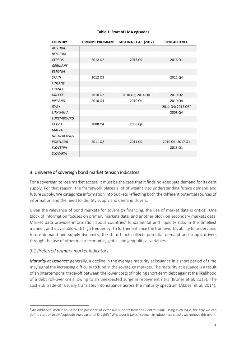
We mark the start of a LMA event in our dataset by whichever event from the three definitions
materialized first. For Greece and Ireland, all three definitions materialized simultaneously in 2010.
According to the above definitions, since 2000 Q1 there have been LMA episodes in 9 euro area
countries. Starting dates by definition are shown in Table 1.6
Given our interest in forecasting sovereign bond market tensions up to one year ahead, we transform
our LMA variable into a pre-LMA dummy the following way. We create a dummy to which we assign a
“1” in the four quarters preceding LMA episodes and we assign a value 0 in the remaining periods. In
addition, we exclude high market access tension periods and four quarters following these periods from
our analysis to avoid post-crisis bias (Bussiere & Fratzscher, 2006). In a robustness exercise, we also
perform the analysis excluding episodes identified using the spread level.
4 To confirm whether the identified suspect LMA cases are indeed LMA, they further investigate explanations for lack of issuance such as lack of funding needs and prefunding. 5 The chosen level threshold corresponds to 92.7 percentile of the spread distribution, which indicates spread levels beyond
350 basis points fall into extreme values of the distribution and could be understood as market tensions. We also tried with a country specific approach, as in Baldacci et al. (2011). We used two standard deviations above a country’s historical rolling average of the spread as our definition. In Figure A5 in the appendix, we show that this approach delivers distress episodes even for countries which clearly did not experience any, such as Austria or Netherlands.
6 Figure A3 in the Appendix provides an overview of LMA episodes by country and definition.
4
Table 1: Start of LMA episodes
COUNTRY ESM/IMF PROGRAM GUSCINA ET AL. (2017) SPREAD LEVEL
AUSTRIA
BELGIUM
CYPRUS 2012 Q2 2013 Q2 2016 Q1
GERMANY
ESTONIA
SPAIN 2012 Q3
2011 Q4
FINLAND
FRANCE
GREECE 2010 Q2 2010 Q2; 2014 Q4 2010 Q2
IRELAND 2010 Q4 2010 Q4 2010 Q4
ITALY
2011 Q4; 2012 Q37
LITHUANIA
2008 Q4
LUXEMBOURG
LATVIA 2008 Q4 2008 Q4
MALTA
NETHERLANDS
PORTUGAL 2011 Q2 2011 Q2 2010 Q4; 2017 Q1
SLOVENIA
2013 Q1
SLOVAKIA
3. Universe of sovereign bond market tension indicators
For a sovereign to lose market access, it must be the case that it finds no adequate demand for its debt
supply. For that reason, the framework places a lot of weight into understanding future demand and
future supply. We categorize information into buckets reflecting both the different potential sources of
information and the need to identify supply and demand drivers.
Given the relevance of bond markets for sovereign financing, the use of market data is critical. One
block of information focuses on primary markets data, and another block on secondary markets data.
Market data provides information about countries’ fundamental and liquidity risks in the timeliest
manner, and is available with high frequency. To further enhance the framework´s ability to understand
future demand and supply dynamics, the third block collects potential demand and supply drivers
through the use of other macroeconomic, global and geopolitical variables.
3.1 Preferred primary market indicators
Maturity at issuance: generally, a decline in the average maturity at issuance in a short period of time
may signal the increasing difficulty to fund in the sovereign markets. The maturity at issuance is a result
of an intertemporal trade-off between the lower costs of holding short-term debt against the likelihood
of a debt roll-over crisis, owing to an unexpected surge in repayment risks (Broner et al, 2013). The
cost-risk trade-off usually translates into issuance across the maturity spectrum (Abbas, et al, 2014).
7 An additional metric could be the presence of extensive support from the Central Bank. Using such logic, for Italy we can define start of an LMA episode the quarter of Draghi’s “Whatever it takes” speech. In robustness checks we remove this event.

5
Therefore, excessive reliance on short-term debt may expose the government to volatile and potentially
increasing debt costs if financial market conditions tighten quickly.
Share of bill financing: a sudden shift to bill issuance may signal that the treasury finds it increasingly
difficult to finance through medium- and long-term bonds given the size of gross financing needs.
During the European debt crisis, the share of bill issuance temporarily increased in larger issuers, such
as Germany, France and Italy, and was the only instrument issued by most countries that entered an
EFSF/ESM financial assistance programme.
Issuance patterns: shifting away from the standard funding practices – competitive auctions of debt
instruments with a fixed coupon, long maturities, and local currency denomination may reflect changes
in macroeconomic conditions and investor sentiment (De Broeck & Guscina 2011), such as a
manifestation of structural shifts in fiscal policy imperatives and sovereign borrowing needs, currency
regimes, financial market architecture, and financial market conditions (Abbas, et al, 2014).
Nevertheless, bonds with various currencies and coupon features can be helpful to expand and
maintain the investor base and diversify funding sources.8
Distribution methods (syndications and private placements): the aim of syndications is to issue new
benchmarks and/or raise relatively larger amounts. Their use may reflect the quality of market access
of the issuers. De Broeck & Guscina (2011) documented that the 2007-2008 financial crisis led to an
increasing use of syndications as a distribution method in a number of euro area countries, such as
Greece, Cyprus, Belgium, Finland, and so on. In an ideal situation, an analysis of the investor base in
these transactions and of the new issue premium the treasuries pay would help to evaluate the quality
of market access. Private placements can be tailor-made to meet the needs of specific types of investors
and to maintain the investor base. This distribution method is only occasionally used in some small
issuers (such as Cyprus and Ireland) and not utilized in countries with solid market access (Germany).
Pace of issuance relative to targets: a slower-than-usual issuance pace may reflect the increased
difficulty of placing bonds in the prevailing market conditions.
Auction frequency: treasuries usually have a pre-determined funding schedule. Changes in auction
frequency may be used to meet structural/temporary variations in funding needs. A marked deviation
from the usual pattern, either an increase or decrease of the number of auctions, may hint at weakened
market access. De Broeck & Guscina (2011) documented an increased number of auctions in almost all
euro area countries during the European debt crisis compared to pre-crisis periods as a result of
elevated gross financing needs.
Auction volume: treasuries usually come to markets with a pre-determined schedule for their bond
auctions. A deviation from the usual pattern, either an increase or decrease of the accepted volume of
auctions, can be a warning sign.
Auction tail: it is the difference between the accepted average and minimum prices, or the difference
between average and maximum accepted yields. A large auction tail in general is not a good sign, as
8 Portugal is an example of increased use of floating coupon bonds in the run-up to LMA in 2010 Q4. In November 2010 Portugal issued 10-year floating coupon bonds at more than 6% despite the total size was small - below €500 million. Shortly after, in February 2011, the issuance of a fixed coupon bond at 6.4% was deemed an unsustainable funding cost, triggering the formal request for an official program.

6
the marginal buyer is only willing to pay a lower price than the average for additional allotment.9 But
this measure can be noisy (auction tails can be large because of a few aggressive bidders).
Auction overbidding: it is the difference between the average price at which a bond is sold at an auction
and the market price of that bond at the auction bidding deadline. If the auctioned price is higher than
the prevailing market price at bidding deadline, there is overbidding; in the opposite case, there is
underbidding. In general, the higher the overbidding vs prior auctions, the stronger an auction is
deemed to be.
New issue premium: this measures the difference between primary accepted prices and secondary fair
prices. Generally, higher new issue premium means the treasuries will need to pay more given a
desirable amount of new issues. But the estimation of fair value is model specific and it is hard to
compile historical data on it across countries based on public information.
Auction cycle/Concession: Secondary market yields rise preceding auctions and decline afterwards. This
affects the cost of the auctions in the primary market and they may provide an indication of the
potential roll-over risk associated with the public debt (Beetsma et al., 2018). Typically, a rise in
secondary yields before an auction signals good demand for that auction.
Auction cancellation/delay: auction cancellation can be a result of a pre-funding (e.g. end of year
cancellations) and an auction can be delayed in order to avoid heightened market volatilities.
Bid-to-cover ratio: this measures over-subscription from investors (demand) relative to supply.
Generally, the higher it is, the better the auction. Beetsma et al. (2018) find that more successful
auctions of euro area public debt, as captured by higher bid-to-cover ratios, lead to lower secondary-
market yields following the auctions. .However, the reliability of this indicator is debatable: (1) bid-to-
cover ratios can be inflated due to market design (the way auctions are organized); (2) when a treasury
issue several bonds in a day, it can play with the allotment, making individual bid-to-cover less reliable.
Auction allotment relative to indicative targets: this compares actual allotment to targeted size or
range. Treasuries face a trade-off between announcing a high target, which increases the chance that
a given auction fails and yields are driven up, and announcing a low target, which forces them to more
frequently organize auctions, and incur the associated costs and risks (Beetsma et al., 2018). If the
issuer does not receive enough bids to cover the desirable allotment, it is a sign of weak demand. If the
increase in size results in weaker pricing, it is likely the issuer is attempting to ‘stuff’ the market.
Ratio of non-competitive allotment to total accepted amount: generally, a certain percentage of
competitive allotment is made available for (selected) primary dealers to submit non-competitive bids
within a short time window, such as one day or two. Presumably, the higher the ratio is, the stronger
the investor demand, as primary dealers could not buy sufficiently either in the auctions and/or from
the prevailing secondary markets.
3.2 Preferred secondary market indicators
Yield curve: Using yields of short- and long-term maturities, we can construct the yield curve of interest
rates. A rapid increase in the short-term rates relative to long-term ones, resulting in a flat or an
inverted curve, generally signals elevated near-term risks. Estrella & Mishkin (1998), Bordo & Haubrich
(2008) and Gerlach & Stuart (2018), among others, show that slope of the yield curve has predictive
9 Some auctions are run as “Dutch auctions” in which uniform price is applied, and therefore no auction tails are observed.

7
power for US growth10. The yield curve also affects the maturity of debt a government will choose to
supply. In times of rising short-term rates, a country will likely issue debt over longer maturities and
vice versa (Broner & Lorenzoni).
Spreads of sovereign bond yields: sovereign spreads are the most widely used measures in the
academia and markets, and are typically monitored to evaluate the overall risk premium emerging from
credit, liquidity and political uncertainties (Guscina, Malik & Papaioannou, 2017). Typically, a sharp
increase in sovereign yield levels and spreads indicates an increased sovereign stress as investors
demand extra premium to hold such securities. This will lead to the shortening of debt maturity issued
by the sovereign (Arellano & Ramanarayanan, 2012).
Bid-ask spreads: the bid-ask spread measures the costs of hypothetically carrying out small round trip
trades. Basically, it informs the market participant how much one needs to pay to buy one security and
immediately sell it back (in the secondary market). Generally, a higher level of bid-ask spreads indicates
a relatively high degree of illiquidity. Bid-ask spreads capture a price dimension, rather than a quantity
dimension, of market liquidity.11
CDS prices: a sovereign CDS contract provides protection against the default of the underlying
sovereign. A sharp increase in CDS prices generally signals the increased risk of sovereign default
(Guscina, Malik & Papaioannou, 2017). 5-year Senior USD CDS is arguably the most liquid and mostly
traded CDS instrument in the markets.12
Trading volume: the level of trading volume in a security or its turnover (volume divided by the
outstanding amount of that security) is used as an indicator of market liquidity of a sovereign bond.
Trading volume tends to increase when new information reaches the market, typically a time of higher
market volatility and concomitantly wide bid-ask spreads. Therefore, turnover can be high when trading
costs increase (i.e. if there is turmoil around political elections).
Bond forwards: periods of high expected yield represent increased costs for future government debt
issuance. In order to optimize costs, a country will likely increase its debt supply in immediate future
and as such prefund for the upcoming periods of increased costs. To capture this effect, one can collect
forward rates of the 10-year bonds in three months’ time and calculate forward premium/discount as
the difference between the forward rate and current ten-year yield, as well as difference between this
forward rate and the benchmark rate, which during our sample period is the best performer’s ten-year
forward rate.
Investor base: monitoring investor holdings by residence and sector helps to assess sovereign market
access from a complementary angle. Evidence shows that the changing dynamics in sectoral investor
base is associated with sovereign yield dynamics (Arslanalp & Poghosyan 2014, Hauner & Kumar 2006,
Jaramillo & Zhang 2013). A rapid sell-off by foreign investors is often an underlying driver of sharp pick-
up in yields and spreads, which can quickly jeopardize a sovereign’s market access.
3.3 Other demand and supply factors
10 Estrella & Hardouvelis (1991) argue that the slope of the yield curve has extra predictive power over the index of leading indicators, real short‐term interest rates, lagged growth in economic activity, and lagged rates of inflation. 11 The size of bid-ask spreads is structurally different among countries, reflecting variations in the depth and market design. 12 The spread between USD and euro-denominated CDS prices and different vintages of CDS contracts, if data are available, can potentially be used as a measure of redenomination risk.

8
Growth outlook: We aim to capture this using GDP growth and growth expectations. Alesina et al. 1992)
and Bernoth et al., (2004) argued that sovereign debt becomes riskier during periods of economic
slowdown. Therefore, an increase (reduction) in growth performance is assumed to improve
(deteriorate) creditworthiness.
Risk aversion: We approximate investor risk aversion by means of the VIX index and its European
equivalent, the V2X index. Since these indices capture expected future market volatility, they can be
used as a proxy for appetite of investors for safe assets, i.e. sovereign bonds, given the flight to quality
phenomenon (Baur and Lucey, 2009). We additionally include the MOVE index, the US Treasury option
implied volatility index produced by Merrill Lynch. The MOVE index can thus serve as a proxy for
investor appetite for other safe assets, such as non-US government bonds.
Sentiment and uncertainty: To account for investor sentiment and uncertainty perceptions vis-à-vis a
country’s economic policy, we use the European Commission’ sentiment index13 (Gelper and Croux,
2009) as well as the Economic Policy Uncertainty index (Baker et al, 2016).
Expected financing needs: In principle, countries with larger financing needs will be more dependent
on bond markets. Beyond a certain level, the larger this future supply, the more jittery markets become.
In order to operationalize this concept, we put together information regarding expected deficits and
refinancing needs.14 This flow measure should provide more information, compared to the stock
measure, on a sovereign’s likelihood of distress (Gabriele et al, 2017).
Future redemptions profile: Countries with large amounts of maturing debt have greater funding needs
and potentially are at risk of not meeting them via debt issuance. This will probably lead to heightened
roll-over risks, which are higher when the maturity profile is concentrated on or around a particular
maturity and when the maturity profile is short with large individual redemptions (Jonasson and
Papaioannou, 2018). We capture amounts of maturing debt over the following three years as share of
total maturing debt over the next ten years, as well as debt maturing in the medium term (four to six
years) and in the long term (eight to ten years).
Bank CDS and public bailouts (contingent liabilities): this captures implicit liabilities materializing in
adverse scenarios. Following bank crises, contingent liabilities from the banking sector could be a
significant determinant of sovereign risk (Arslanalp and Liao, 2014). We collect data on bank bailouts
by governments and CDS prices of banks active within a country. These indicators capture government
costs related to domestic banks’ distress and represent an additional funding need for a country.
Banking sector index: a country-level index measuring the performance of average banking equity
prices weighted by market capitalization on the same day. Generally, increases in the index indicate
positive investor sentiment towards that country’s banking sector. Sovereign and banking distress feed
into each other, with balance sheet interconnections, credit dynamics, financial openness and
economic growth being important ((Erce and Balteanu 2017, Del’Ariccia et al. 2018).
Stock market index: the performance of the stock market informs about investor sentiment on the state
of the economy. Generally, increases in stock market indices signal positive investor sentiment. Also,
13Available at: https://ec.europa.eu/info/business-economy-euro/indicators-statistics/economic-databases/business-and-consumer-surveys_en 14 We approximate a country’s expected financing needs over the next year as the sum of the expected deficit for that year
(we assume it is the same as the current year’s deficit) and future debt redemptions over the same year.

9
volatilities in stock markets can be related to variations in the underlying macroeconomic factors, such
as GDP growth, inflation and short-term interest rates (Engel and Rangel, 2007).
Cash position: indicative of a sovereign’s need for financing through debt markets. Large cash or
liquidity reserves lower the need for a government to issue debt. Sovereign debt managers view a
liquidity buffer as an effective tool to address re-financing risk and liquidity risk that may arise for
reasons such as unexpected increases in borrowing needs, short-term mismatches in fiscal cash flows
or the temporary loss of market access (OECD, 2018).
Fiscal outlook: Indicators capturing fiscal position, debt/GDP and deficit/GDP, provide a picture of how
much a country will need to raise to finance its position. Projections of key fiscal variables should help
to inform the fiscal sustainability risks associated with a government’s possible inability to roll over its
outstanding stock of debts (Baldacci et al. 2011).
Shocks to foreign investors: Negative shocks to a government’s bondholders adversely affect their
demand for government bonds. We proxy these shocks using GDP growth in large countries. Therefore
we assume that if there is a negative output shock, their shares of debt holdings will increase.
4. Collecting and transforming the data
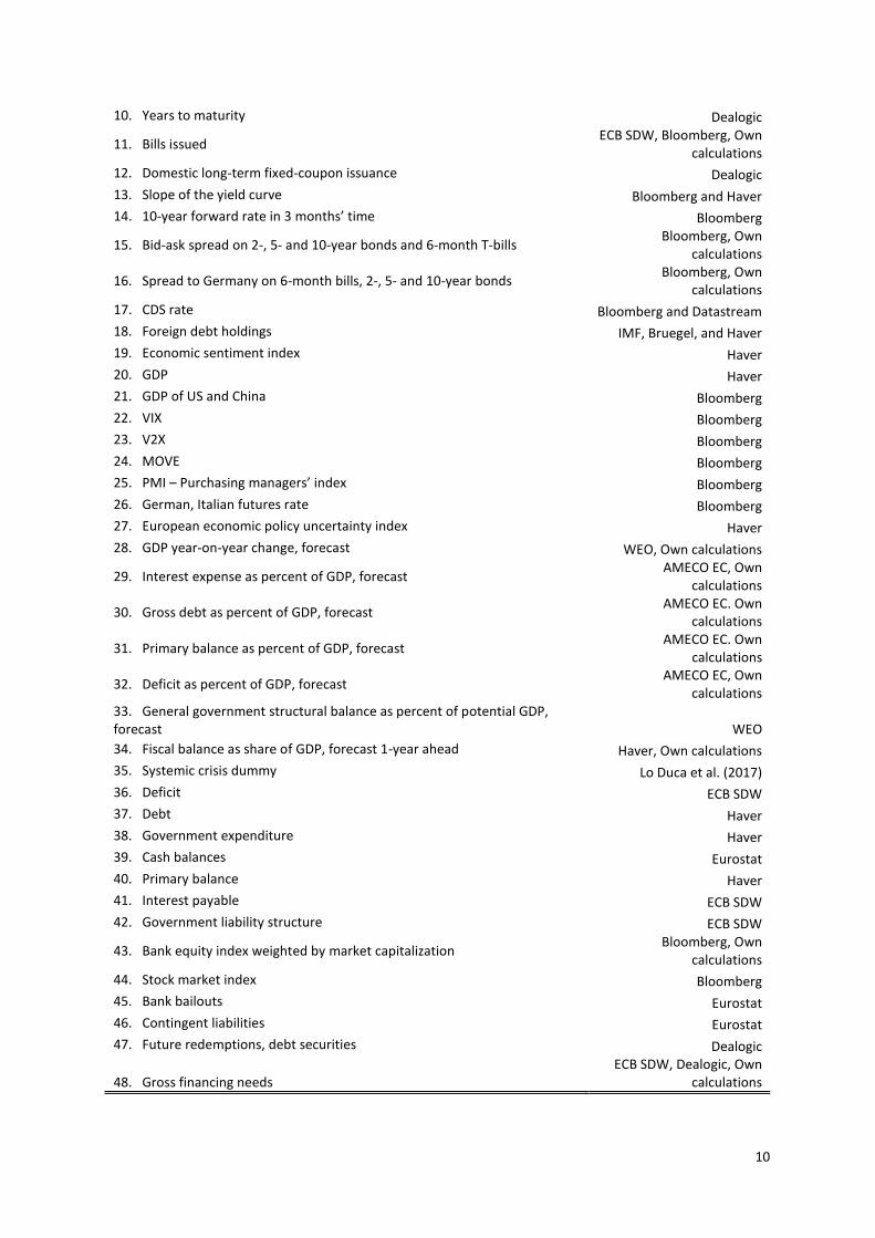
We collected 48 raw underlying indicators, listed in Table 2, from primary and secondary markets,
capturing global demand and government supply, for 19 euro area countries. We generated
transformations of these indicators to capture proportions on debt issuance, share of GDP, moving
averages over one and two years, differences to these moving averages, standard deviation and
skewness of selected indicators over moving one-year horizon, as well as per current period, year-on-
year differences, and differences compared to Germany and the best performing country. The
transformations yielded 242 variables altogether.
Several indicators such as bid-to-cover ratios, PMI, Italian futures rate, the forecast of fiscal balance as
share of GDP, and forecast of general government structural balance as a percent of potential GDP
suffer from serious data limitations in the form of either short time series or restricted availability across
countries. Thus, we exclude them from further analysis. We also exclude yield spreads to Germany on
6-month T-bills, 2-year, 5-year and 10-year sovereign bonds since these overlap with our definition of
LMA episodes. We also eliminate Cyprus, Estonia, Malta, Lithuania and Luxembourg due to significant
data limitations across indicators from primary and secondary markets, global demand and government
supply side. All the indicators and their transformations were lagged by one quarter to account for data
publication lags.
Table 2. Underlying data and sources
1. Bid-to-cover on 6-month government bills Bloomberg
2. Bid-to-cover on 10-year government bonds Bloomberg
3. Syndicated issuance Dealogic
4. Foreign currency issuance Dealogic
5. Floating coupon issuance Dealogic
6. Inflation-linked issuance Dealogic
7. Volume issued Dealogic
8. Number of issuances Dealogic
9. Yield to maturity Dealogic
10
10. Years to maturity Dealogic
11. Bills issued ECB SDW, Bloomberg, Own
calculations
12. Domestic long-term fixed-coupon issuance Dealogic
13. Slope of the yield curve Bloomberg and Haver
14. 10-year forward rate in 3 months’ time Bloomberg
15. Bid-ask spread on 2-, 5- and 10-year bonds and 6-month T-bills Bloomberg, Own
calculations
16. Spread to Germany on 6-month bills, 2-, 5- and 10-year bonds Bloomberg, Own
calculations
17. CDS rate Bloomberg and Datastream
18. Foreign debt holdings IMF, Bruegel, and Haver
19. Economic sentiment index Haver
20. GDP Haver
21. GDP of US and China Bloomberg
22. VIX Bloomberg
23. V2X Bloomberg
24. MOVE Bloomberg
25. PMI – Purchasing managers’ index Bloomberg
26. German, Italian futures rate Bloomberg
27. European economic policy uncertainty index Haver
28. GDP year-on-year change, forecast WEO, Own calculations
29. Interest expense as percent of GDP, forecast AMECO EC, Own
calculations
30. Gross debt as percent of GDP, forecast AMECO EC. Own
calculations
31. Primary balance as percent of GDP, forecast AMECO EC. Own
calculations
32. Deficit as percent of GDP, forecast AMECO EC, Own
calculations 33. General government structural balance as percent of potential GDP, forecast WEO
34. Fiscal balance as share of GDP, forecast 1-year ahead Haver, Own calculations
35. Systemic crisis dummy Lo Duca et al. (2017)
36. Deficit ECB SDW
37. Debt Haver
38. Government expenditure Haver
39. Cash balances Eurostat
40. Primary balance Haver
41. Interest payable ECB SDW
42. Government liability structure ECB SDW
43. Bank equity index weighted by market capitalization Bloomberg, Own
calculations
44. Stock market index Bloomberg
45. Bank bailouts Eurostat
46. Contingent liabilities Eurostat
47. Future redemptions, debt securities Dealogic
48. Gross financing needs ECB SDW, Dealogic, Own
calculations

11
Adding normalized transformations. To increase the ability of our indicators to predict market distress,
we also built transformations comparing indicator dynamics to either country-specific history or
against-peers at a point in time. We also add normalized forms of the indicators and their
transformations both within and across countries. We based the normalization of individual indicators
on comments from ESM Funding and Investment teams, reading of the relevant literature and the
indicators’ dynamics.15
After extending the set of indicators and their transformations with their normalized transformations
both by country and across countries, the final dataset comprises 657 indicators altogether.
5. Univariate (signalling) analysis of indicators
To identify indicators most suitable for signalling increased sovereign bond market tensions, we
evaluate the usefulness of all the collected indicators individually. For this purpose we employ signalling
analysis as well as calculate area under receiver operating characteristic curve (AUROC) on data until
2011 Q2. The data after this point we reserve for out-of-sample testing.
In the signalling approach, a warning signal is issued when an indicator exceeds a threshold, which we
define by a particular percentile of an indicator’s own cross-country distribution. This approach
assumes an extreme non-linear relationship between the indicator and the event to be predicted. Each
quarter for each indicator falls into one of the four quadrants of the matrix below.
Table 3: Classification matrix
Loss of market access No loss of market access
Signal issued True positive False positive (False alarm)
No signal issued False negative (Missed event) True negative
Missed events rate (Type I) error can be obtained by dividing the number of missed events by the
number of periods in which sovereign bond market tensions were high:
𝑇𝑦𝑝𝑒 𝐼 =∑ 𝐹𝑎𝑙𝑠𝑒 𝑛𝑒𝑔𝑎𝑡𝑖𝑣𝑒
∑ 𝐹𝑎𝑙𝑠𝑒 𝑛𝑒𝑔𝑎𝑡𝑖𝑣𝑒 + ∑ 𝑇𝑟𝑢𝑒 𝑝𝑜𝑠𝑖𝑡𝑖𝑣𝑒
False alarm rate (Type II error) can be calculated by dividing the number of false alarms by the number
of periods in which there were no high sovereign bond market tensions:
𝑇𝑦𝑝𝑒 𝐼𝐼 =∑ 𝐹𝑎𝑙𝑠𝑒 𝑝𝑜𝑠𝑖𝑡𝑖𝑣𝑒
∑ 𝐹𝑎𝑙𝑠𝑒 𝑝𝑜𝑠𝑖𝑡𝑖𝑣𝑒 + ∑ 𝑇𝑟𝑢𝑒 𝑛𝑒𝑔𝑎𝑡𝑖𝑣𝑒
Following Alessi and Detken (2011) we calculate the overall utility of each indicator using the function:
U = min(𝜃; 1 − 𝜃) − 𝜃𝐹𝑁
(𝐹𝑁+𝑇𝑃)+ (1 − 𝜃)
𝐹𝑃
(𝐹𝑃+𝑇𝑁), where
𝐿 = 𝜃𝐹𝑁
(𝐹𝑁+𝑇𝑃)+ (1 − 𝜃)
𝐹𝑃
(𝐹𝑃+𝑇𝑁),
15 Normalization results in loss of observations for some indicators where we choose to stress country-specific dynamics.
Floating coupon issuance share and foreign currency issuance share are examples of such indicators. These indicators manifest zero variance until 2011 Q2. To preserve as many observations as possible, we do not normalize indicators with zero variance.
(1)
(2)
(3)
(4)
12
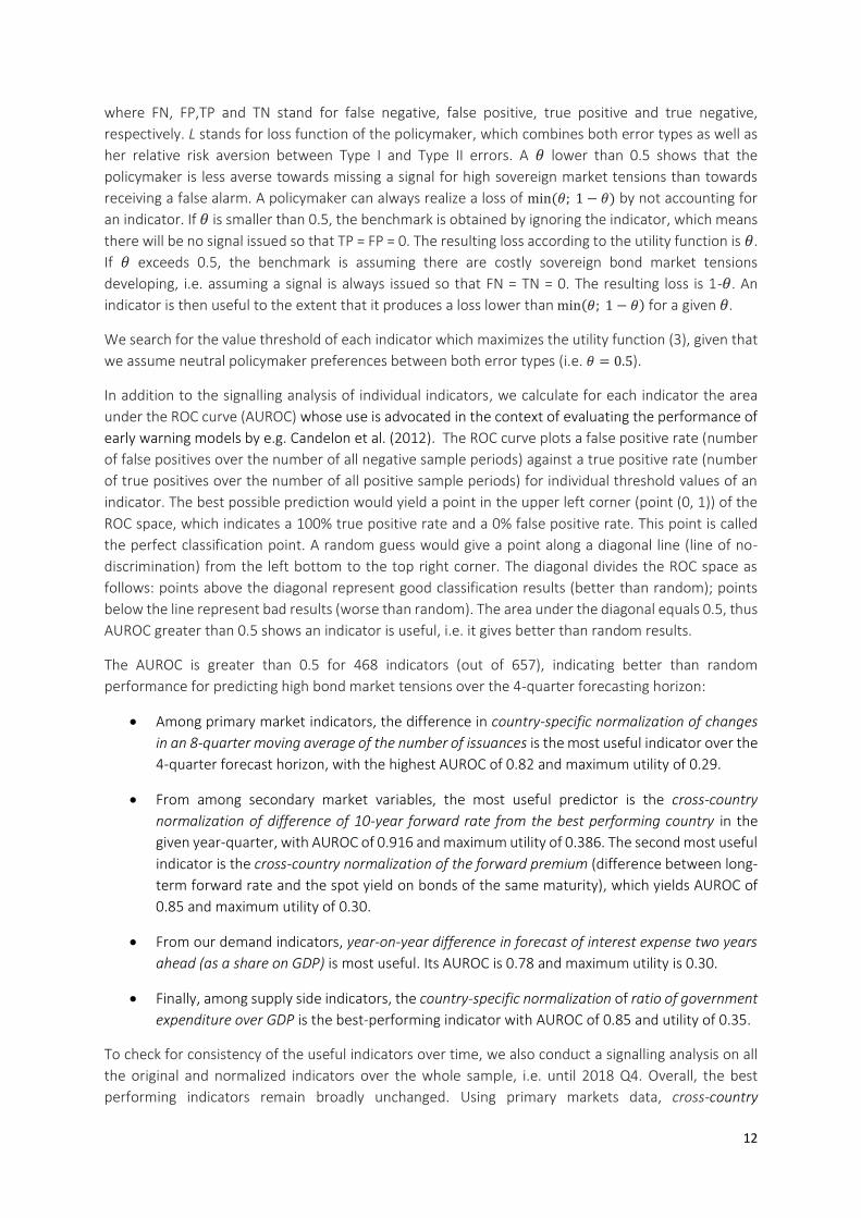
where FN, FP,TP and TN stand for false negative, false positive, true positive and true negative,
respectively. L stands for loss function of the policymaker, which combines both error types as well as
her relative risk aversion between Type I and Type II errors. A 𝜃 lower than 0.5 shows that the
policymaker is less averse towards missing a signal for high sovereign market tensions than towards
receiving a false alarm. A policymaker can always realize a loss of min (𝜃; 1 − 𝜃) by not accounting for
an indicator. If 𝜃 is smaller than 0.5, the benchmark is obtained by ignoring the indicator, which means
there will be no signal issued so that TP = FP = 0. The resulting loss according to the utility function is 𝜃.
If 𝜃 exceeds 0.5, the benchmark is assuming there are costly sovereign bond market tensions
developing, i.e. assuming a signal is always issued so that FN = TN = 0. The resulting loss is 1-𝜃. An
indicator is then useful to the extent that it produces a loss lower than min(𝜃; 1 − 𝜃) for a given 𝜃.
We search for the value threshold of each indicator which maximizes the utility function (3), given that
we assume neutral policymaker preferences between both error types (i.e. 𝜃 = 0.5).
In addition to the signalling analysis of individual indicators, we calculate for each indicator the area
under the ROC curve (AUROC) whose use is advocated in the context of evaluating the performance of
early warning models by e.g. Candelon et al. (2012). The ROC curve plots a false positive rate (number
of false positives over the number of all negative sample periods) against a true positive rate (number
of true positives over the number of all positive sample periods) for individual threshold values of an
indicator. The best possible prediction would yield a point in the upper left corner (point (0, 1)) of the
ROC space, which indicates a 100% true positive rate and a 0% false positive rate. This point is called
the perfect classification point. A random guess would give a point along a diagonal line (line of no-
discrimination) from the left bottom to the top right corner. The diagonal divides the ROC space as
follows: points above the diagonal represent good classification results (better than random); points
below the line represent bad results (worse than random). The area under the diagonal equals 0.5, thus
AUROC greater than 0.5 shows an indicator is useful, i.e. it gives better than random results.
The AUROC is greater than 0.5 for 468 indicators (out of 657), indicating better than random
performance for predicting high bond market tensions over the 4-quarter forecasting horizon:
Among primary market indicators, the difference in country-specific normalization of changes
in an 8-quarter moving average of the number of issuances is the most useful indicator over the
4-quarter forecast horizon, with the highest AUROC of 0.82 and maximum utility of 0.29.
From among secondary market variables, the most useful predictor is the cross-country
normalization of difference of 10-year forward rate from the best performing country in the
given year-quarter, with AUROC of 0.916 and maximum utility of 0.386. The second most useful
indicator is the cross-country normalization of the forward premium (difference between long-
term forward rate and the spot yield on bonds of the same maturity), which yields AUROC of
0.85 and maximum utility of 0.30.
From our demand indicators, year-on-year difference in forecast of interest expense two years
ahead (as a share on GDP) is most useful. Its AUROC is 0.78 and maximum utility is 0.30.
Finally, among supply side indicators, the country-specific normalization of ratio of government
expenditure over GDP is the best-performing indicator with AUROC of 0.85 and utility of 0.35.
To check for consistency of the useful indicators over time, we also conduct a signalling analysis on all
the original and normalized indicators over the whole sample, i.e. until 2018 Q4. Overall, the best
performing indicators remain broadly unchanged. Using primary markets data, cross-country

13
normalization of changes in an 8-quarter moving average of the number of issuances is the best
predictor with AUROC of 0.732 but a quite high Type II error rate of 0.4. Using secondary markets data,
cross-country normalization of difference of the 10-year forward rate from the best performing country
remains the most useful indicator, with AUROC of 0.936 and utility of 0.397. Within demand and supply
side indicators, year-on-year growth in the inverse of a 4-quarter moving average of the banking sector
index is the most useful indicator with utility of 0.301 and AUROC of 0.846. The second most useful
indicator is cross-country normalization of the year-on-year difference in debt-to-GDP ratio with AUROC
of 0.83 and utility of 0.25.
5.1 Selection of the indicators to be monitored
Following the results of the signalling analysis, we proceed to identify and pre-select the most useful
indicators on a univariate basis for further use within a multivariate framework. For this purpose, we
use the area under the ROC curve and Type I and Type II error rates calculated for each indicator in a
univariate analysis on the sample ending in 2011 Q2.
First, we discard indicators whose AUROC, a global measure of usefulness to predict periods leading to
high sovereign bond market tensions, does not exceed 0.5; the number corresponding to an indicator
yielding random results. Next, we discard those indicators for which either Type I or Type II error equals
or exceeds 0.4. That is we exclude indicators that either fail to issue a signal or emit false alarms in 40
percent and more quarters of high tension episodes or tranquil periods, respectively. Subsequently, we
select the best performing transformation of the underlying indicator that meets both of the above
criteria: AUROC above 0.5 and Type I and Type II error below 0.4. These conditions leave us with
substantially reduced sets of useful univariate indicators, especially from the primary markets. For this
reason, we also consider such transformations of the primary market indicators that do not strictly
meet the error type condition, but have AUROC and usefulness sufficiently high and which outperform
other primary market indicators. Similarly, we retain the best performing transformations of the V2X
index and US GDP growth in order to control for global demand factors. On the supply side, best
performing transformations of GDP growth forecast and gross financing needs were retained to ensure
comprehensiveness. Table 4 presents the set of the best-performing indicators.
The set of the most useful indicators contains the following transformations of the raw indicators:
Primary market: country-specific normalization of difference in moving average of number of
issuances over 8 quarters, country-specific normalization of ratio of bills issuance to GDP, cross-
country normalization of difference in moving average of share of floating coupon issuance
over 8 quarters, cross-country normalization of difference in moving average of share of
syndicated issuance over 8 quarters.
Secondary market: cross-country normalization of bid-ask spread on 2-year bonds, cross-
country normalization of standard deviation of bid-ask spread on 5-year bonds, cross-country
normalization of bid-ask spread on 10-year bonds, cross-country normalization of difference in
foreign-held debt share on total debt, cross-country normalization of difference of 10-year
forward rate from the best-performing country, cross-country normalization of forward
premium, cross-country normalization of year-on-year difference in CDS rate.
Supply and global demand indicators: year-on-year difference in forecast of interest expense
share on GDP in two years, cross-country normalization of European economic uncertainty
14
index, cross-country normalization of US GDP growth, cross-country normalization of V2X
index, cross-country normalization of year-on-year difference in stock market index, cross-
country normalization of difference in GDP growth forecast in three years, cross-country
normalization of difference in gross debt over GDP forecast in a year, country-specific
normalization of government expenditure over GDP, cross-country normalization of year-on-
year difference in debt-to-GDP ratio, cross-country normalization of difference in interest
payable to GDP, cross-country normalization of rate of change in banking sector index
(weighted average of bank equity prices by market capitalization), cross-country normalization
of difference in 4-quarter moving average of gross financing needs over GDP, cross-country
normalization of difference in bailouts to GDP.
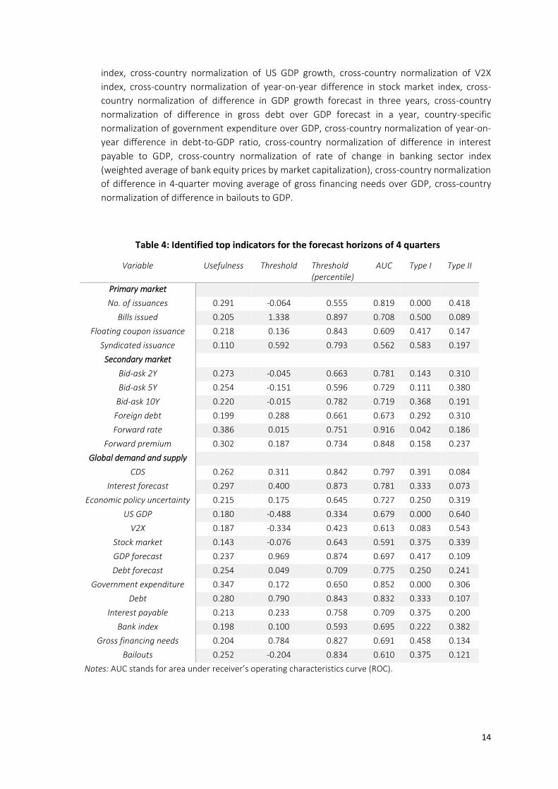
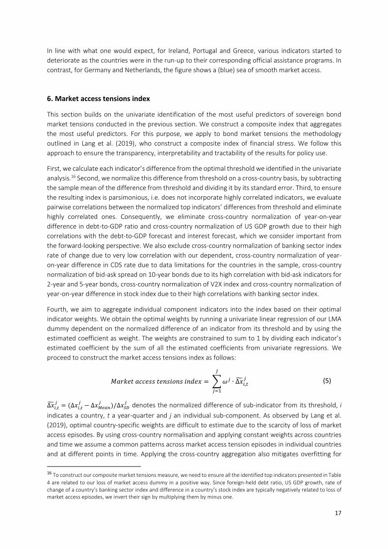
Table 4: Identified top indicators for the forecast horizons of 4 quarters
Variable Usefulness Threshold Threshold (percentile)
AUC Type I Type II
Primary market
No. of issuances 0.291 -0.064 0.555 0.819 0.000 0.418
Bills issued 0.205 1.338 0.897 0.708 0.500 0.089
Floating coupon issuance 0.218 0.136 0.843 0.609 0.417 0.147
Syndicated issuance 0.110 0.592 0.793 0.562 0.583 0.197
Secondary market
Bid-ask 2Y 0.273 -0.045 0.663 0.781 0.143 0.310
Bid-ask 5Y 0.254 -0.151 0.596 0.729 0.111 0.380
Bid-ask 10Y 0.220 -0.015 0.782 0.719 0.368 0.191
Foreign debt 0.199 0.288 0.661 0.673 0.292 0.310
Forward rate 0.386 0.015 0.751 0.916 0.042 0.186
Forward premium 0.302 0.187 0.734 0.848 0.158 0.237
Global demand and supply
CDS 0.262 0.311 0.842 0.797 0.391 0.084
Interest forecast 0.297 0.400 0.873 0.781 0.333 0.073
Economic policy uncertainty 0.215 0.175 0.645 0.727 0.250 0.319
US GDP 0.180 -0.488 0.334 0.679 0.000 0.640
V2X 0.187 -0.334 0.423 0.613 0.083 0.543
Stock market 0.143 -0.076 0.643 0.591 0.375 0.339
GDP forecast 0.237 0.969 0.874 0.697 0.417 0.109
Debt forecast 0.254 0.049 0.709 0.775 0.250 0.241
Government expenditure 0.347 0.172 0.650 0.852 0.000 0.306
Debt 0.280 0.790 0.843 0.832 0.333 0.107
Interest payable 0.213 0.233 0.758 0.709 0.375 0.200
Bank index 0.198 0.100 0.593 0.695 0.222 0.382
Gross financing needs 0.204 0.784 0.827 0.691 0.458 0.134
Bailouts 0.252 -0.204 0.834 0.610 0.375 0.121
Notes: AUC stands for area under receiver’s operating characteristics curve (ROC).

15
5.2 Dynamics of the identified top indicators
This subsection investigates the dynamics of the top indicators identified using univariate analysis.
Figure A1 in the appendix shows the median dynamics of each indicator in the four quarters prior to
the start of the loss of market access episodes, as well as in the four quarters following the loss of
market access incidence. The dashed red line represents the median behaviour around LMA episodes
and the shaded area highlights interquartile range or the difference between the 75th and the 25th
percentile of the indicator distribution around LMA episodes. The green line shows the median of the
indicator before the Global Financial Crisis, i.e. in the period from 2003 Q4 until 2005 Q4. The black line
indicates an indicator-specific threshold for issuing signals. Overall, given their observed dynamics,
most selected indicators would issue a signal either during full four quarters leading to the LMA episode
or at least at some point in this four-quarter window. However, four indicators do not show good ability
to correctly signal high stress periods leading to an LMA event: the ratio of bills issuance-to-GDP,
changes in the 8-quarter moving average of syndicated issuance share, year-on-year difference in 3-
years ahead GDP growth forecast, and year-on-year change in 4-quarter moving average of gross
financing needs to GDP. The median dynamics of these indicators during high-tensions pre-LMA periods
are quite close in direction and magnitude to those during tranquil times, and as such, fail to exceed
their indicator-specific thresholds. Consequently, we infer that median dynamics of these indicators
cannot be relied upon to provide a good early warning signal of sovereign market access tensions. This
unsatisfactory performance can be attributed to a relatively large Type I error rate of these four
indicators, i.e. exceeding 0.4, and in the case of the ratio of bills issuance-to-GDP and the changes in
the 8-quarter moving average of syndicated issuance share even exceeding 0.5. Table 5 presents a
detailed list of those quarters in the year preceding the start of LMA episodes per country that were
successfully identified by our selected indicators of market tensions.
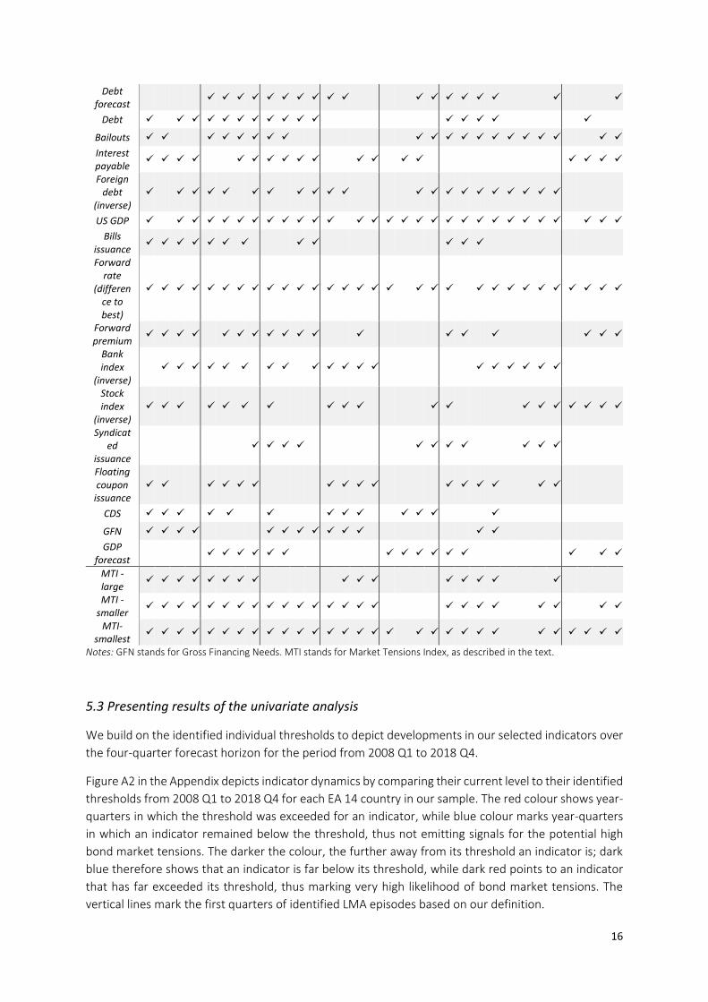
Table 5: Identified periods of up to 4 quarters prior to LMA by top indicators
Spain Greece Ireland Italy Latvia Portugal Slovenia
Quarters before LMA episodes LMA
episode 1 LMA
episode 2
4 3 2 1 4 3 2 1 4 3 2 1 4 3 2 1 4 3 2 1 4 3 2 1 4 3 2 1 4 3 2 1
Interest forecast
No. of issuance
s
Government
expenditure
Bid-ask 2Y
Bid-ask 10Y
Bid-ask 5Y
volatility
V2X
Economic policy uncertai
nty
16
Debt forecast
Debt
Bailouts
Interest payable
Foreign debt
(inverse)
US GDP
Bills issuance
Forward rate
(difference to best)
Forward premium
Bank index
(inverse)
Stock index
(inverse)
Syndicated
issuance
Floating coupon
issuance
CDS
GFN
GDP forecast
MTI -large
MTI -smaller
MTI-smallest
Notes: GFN stands for Gross Financing Needs. MTI stands for Market Tensions Index, as described in the text.
5.3 Presenting results of the univariate analysis
We build on the identified individual thresholds to depict developments in our selected indicators over
the four-quarter forecast horizon for the period from 2008 Q1 to 2018 Q4.
Figure A2 in the Appendix depicts indicator dynamics by comparing their current level to their identified
thresholds from 2008 Q1 to 2018 Q4 for each EA 14 country in our sample. The red colour shows year-
quarters in which the threshold was exceeded for an indicator, while blue colour marks year-quarters
in which an indicator remained below the threshold, thus not emitting signals for the potential high
bond market tensions. The darker the colour, the further away from its threshold an indicator is; dark
blue therefore shows that an indicator is far below its threshold, while dark red points to an indicator
that has far exceeded its threshold, thus marking very high likelihood of bond market tensions. The
vertical lines mark the first quarters of identified LMA episodes based on our definition.
17
In line with what one would expect, for Ireland, Portugal and Greece, various indicators started to
deteriorate as the countries were in the run-up to their corresponding official assistance programs. In
contrast, for Germany and Netherlands, the figure shows a (blue) sea of smooth market access.
6. Market access tensions index
This section builds on the univariate identification of the most useful predictors of sovereign bond
market tensions conducted in the previous section. We construct a composite index that aggregates
the most useful predictors. For this purpose, we apply to bond market tensions the methodology
outlined in Lang et al. (2019), who construct a composite index of financial stress. We follow this
approach to ensure the transparency, interpretability and tractability of the results for policy use.
First, we calculate each indicator’s difference from the optimal threshold we identified in the univariate
analysis.16 Second, we normalize this difference from threshold on a cross-country basis, by subtracting
the sample mean of the difference from threshold and dividing it by its standard error. Third, to ensure
the resulting index is parsimonious, i.e. does not incorporate highly correlated indicators, we evaluate
pairwise correlations between the normalized top indicators’ differences from threshold and eliminate
highly correlated ones. Consequently, we eliminate cross-country normalization of year-on-year
difference in debt-to-GDP ratio and cross-country normalization of US GDP growth due to their high
correlations with the debt-to-GDP forecast and interest forecast, which we consider important from
the forward-looking perspective. We also exclude cross-country normalization of banking sector index
rate of change due to very low correlation with our dependent, cross-country normalization of year-
on-year difference in CDS rate due to data limitations for the countries in the sample, cross-country
normalization of bid-ask spread on 10-year bonds due to its high correlation with bid-ask indicators for
2-year and 5-year bonds, cross-country normalization of V2X index and cross-country normalization of
year-on-year difference in stock index due to their high correlations with banking sector index.
Fourth, we aim to aggregate individual component indicators into the index based on their optimal
indicator weights. We obtain the optimal weights by running a univariate linear regression of our LMA
dummy dependent on the normalized difference of an indicator from its threshold and by using the
estimated coefficient as weight. The weights are constrained to sum to 1 by dividing each indicator’s
estimated coefficient by the sum of all the estimated coefficients from univariate regressions. We
proceed to construct the market access tensions index as follows:
𝑀𝑎𝑟𝑘𝑒𝑡 𝑎𝑐𝑐𝑒𝑠𝑠 𝑡𝑒𝑛𝑠𝑖𝑜𝑛𝑠 𝑖𝑛𝑑𝑒𝑥 = ∑ 𝜔𝑗 ∙ ∆�̃�𝑖,𝑡𝑗
𝐽
𝑗=1
∆�̃�𝑖,𝑡𝑗
= (∆𝑥𝑖,𝑡𝑗
− ∆𝑥𝑀𝑒𝑎𝑛𝑗
)/∆𝑥𝑆𝐷𝑗 denotes the normalized difference of sub-indicator from its threshold, i
indicates a country, t a year-quarter and j an individual sub-component. As observed by Lang et al.
(2019), optimal country-specific weights are difficult to estimate due to the scarcity of loss of market
access episodes. By using cross-country normalisation and applying constant weights across countries
and time we assume a common patterns across market access tension episodes in individual countries
and at different points in time. Applying the cross-country aggregation also mitigates overfitting for
16 To construct our composite market tensions measure, we need to ensure all the identified top indicators presented in Table
4 are related to our loss of market access dummy in a positive way. Since foreign-held debt ratio, US GDP growth, rate of change of a country’s banking sector index and difference in a country’s stock index are typically negatively related to loss of market access episodes, we invert their sign by multiplying them by minus one.
(5)
18
individual LMA events. Furthermore, constraining the sum of weights of individual subcomponents to
1 allows us to decompose the market access tensions index (MTI) into its drivers at any quarter in our
sample. Figure A4 in the Appendix shows the MTI decomposition for EA 14 countries.
Out of the best performing indicators in Table 4, based on their subpar median dynamics over the start
of loss of market access episodes (see Figure A1 in the Appendix), we exclude from the composite index
the following indicators: ratio of bills issuance-to-GDP, difference in moving average of syndicated
issuance share over the last 2 years, year-on-year difference in GDP growth forecast in 3 years, and
year-on-year difference in moving average of gross financing needs to GDP over previous 4 quarters.17
Due to data constraints, we construct an alternative (smaller) market access tensions index comprising
fewer indicators. Due to data limitations for Ireland, Latvia and Slovenia, we eliminate the two bid-ask
indicators (spread on 2-year bond and volatility of spread on 5-year bond). We then exclude the forward
premium, which is missing for Latvia and Slovenia, and calculate the “smallest” market tensions index,
comprising 10 indicators from Table 4. The calculated optimal weights for individual indicators are
shown in Table 6. Figure 1 compares the dynamics of the “largest” market tensions index (comprising
13 sub-components) with the “smallest” index. While the indices co-move strongly, in most countries
the largest index appears shifted downwards compared to the more parsimonious version. For
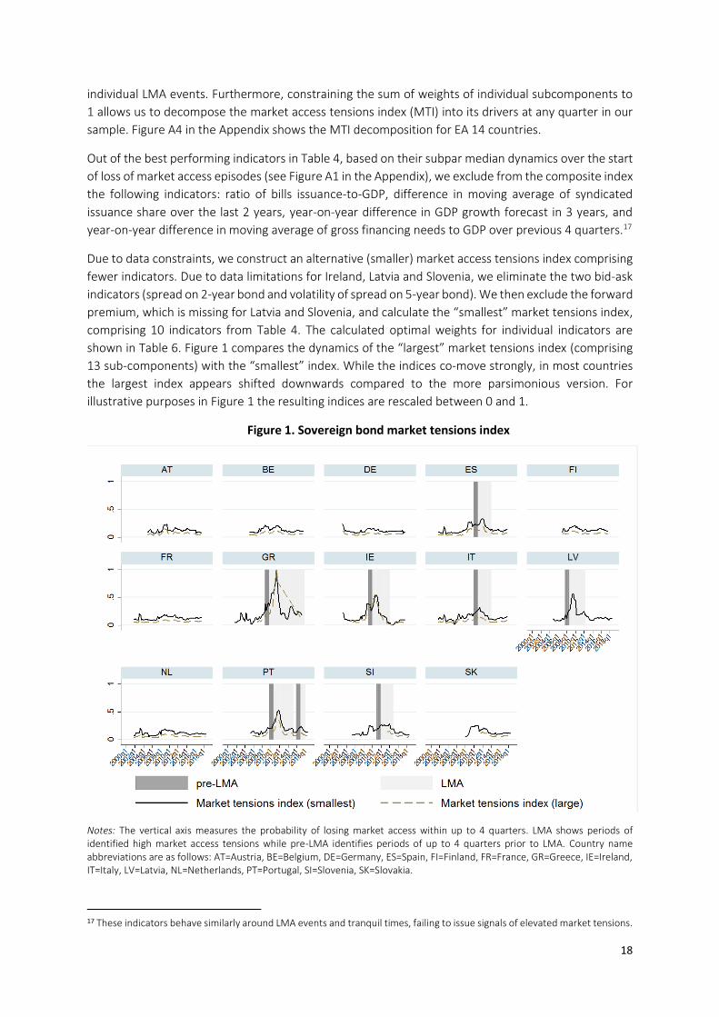
illustrative purposes in Figure 1 the resulting indices are rescaled between 0 and 1.
Figure 1. Sovereign bond market tensions index
Notes: The vertical axis measures the probability of losing market access within up to 4 quarters. LMA shows periods of identified high market access tensions while pre-LMA identifies periods of up to 4 quarters prior to LMA. Country name abbreviations are as follows: AT=Austria, BE=Belgium, DE=Germany, ES=Spain, FI=Finland, FR=France, GR=Greece, IE=Ireland, IT=Italy, LV=Latvia, NL=Netherlands, PT=Portugal, SI=Slovenia, SK=Slovakia.
17 These indicators behave similarly around LMA events and tranquil times, failing to issue signals of elevated market tensions.

19
Table 6: Optimal weights for sub-components of market access tension indices
Sub-component Largest Index
Smaller index
Smallest index
Weight
Primary market
No. of issuances 0.05 0.07 0.07
Bills issued - - -
Floating coupon issuance 0.04 0.06 0.06
Syndicated issuance - - -
Secondary market
Bid-ask 2Y 0.13 - -
Bid-ask 5Y 0.15 - -
Bid-ask 10Y - - -
Foreign debt 0.03 0.04 0.04
Forward rate 0.27 0.37 0.40
Forward premium 0.02 0.03 -
Global demand and supply
CDS - - -
Interest forecast 0.13 0.18 0.18
Economic policy uncertainty 0.02 0.03 0.03
US GDP - - -
V2X - - -
Stock market - - -
GDP forecast - - -
Debt forecast 0.04 0.06 0.06
Government expenditure 0.04 0.06 0.06
Debt - - -
Interest payable 0.04 0.05 0.05
Bank index - - -
Gross financing needs - - -
Bailouts 0.04 0.05 0.05
To evaluate how successful these indices are in capturing tensions in sovereign bond markets, we
compare year-on-year changes in the indices during the four quarters leading to LMA episodes with
those in tranquil periods. We conduct difference-in-means testing to assess if on average the composite
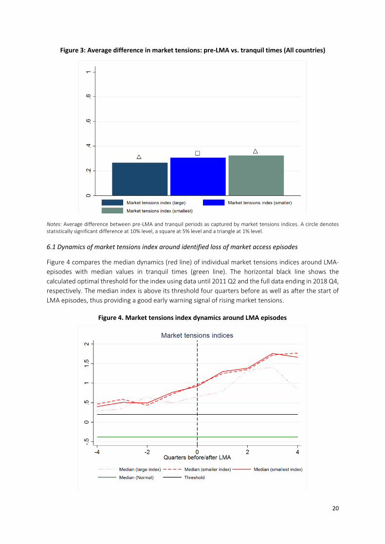
indices succeed in capturing increases in market tensions for individual countries. Figure 3 shows the
results. In all countries that experienced an LMA episode, all three constructed indices of market access
tensions capture increases in market tensions in pre-LMA times. Average increases in market tensions
in pre-LMA times are more positive and statistically significantly different from those in tranquil times
at least at 5% significance level18
18 Statistical significance is depicted by a hollow shape above bars; a circle for significance at 10% level, a square at 5% and a triangle for significance at 1% level.
20
Figure 3: Average difference in market tensions: pre-LMA vs. tranquil times (All countries)
Notes: Average difference between pre-LMA and tranquil periods as captured by market tensions indices. A circle denotes statistically significant difference at 10% level, a square at 5% level and a triangle at 1% level.
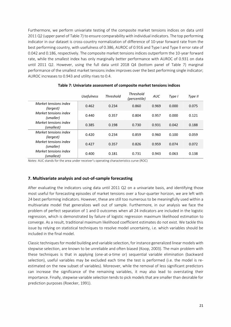
6.1 Dynamics of market tensions index around identified loss of market access episodes
Figure 4 compares the median dynamics (red line) of individual market tensions indices around LMA-
episodes with median values in tranquil times (green line). The horizontal black line shows the
calculated optimal threshold for the index using data until 2011 Q2 and the full data ending in 2018 Q4,
respectively. The median index is above its threshold four quarters before as well as after the start of
LMA episodes, thus providing a good early warning signal of rising market tensions.
Figure 4. Market tensions index dynamics around LMA episodes
21
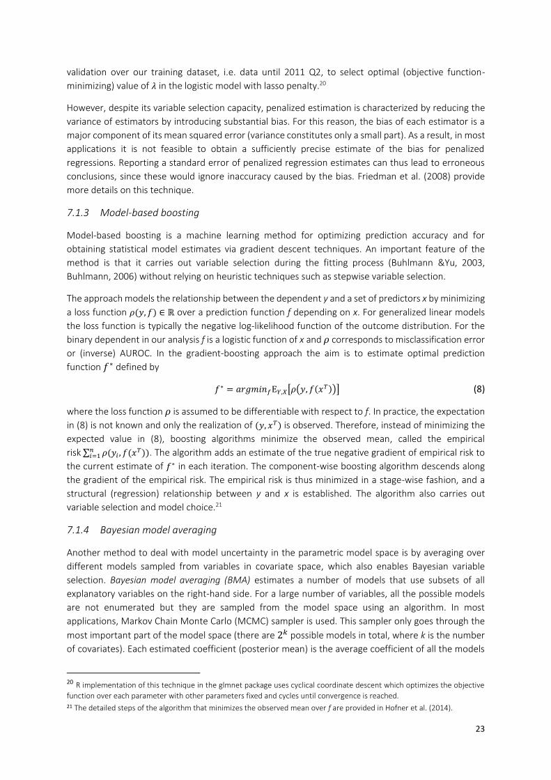
Furthermore, we perform univariate testing of the composite market tensions indices on data until
2011 Q2 (upper panel of Table 7) to ensure comparability with individual indicators. The top performing
indicator in our dataset is cross-country normalization of difference of 10-year forward rate from the
best performing country, with usefulness of 0.386, AUROC of 0.916 and Type I and Type II error rate of
0.042 and 0.186, respectively. The composite market tensions indices outperform the 10-year forward
rate, while the smallest index has only marginally better performance with AUROC of 0.931 on data
until 2011 Q2. However, using the full data until 2018 Q4 (bottom panel of Table 7) marginal
performance of the smallest market tensions index improves over the best performing single indicator;
AUROC increases to 0.943 and utility rises to 0.4.
Table 7: Univariate assessment of composite market tensions indices
Usefulness Threshold Threshold
(percentile) AUC Type I Type II
Market tensions index (largest)
0.462 0.234 0.860 0.969 0.000 0.075
Market tensions index (smaller)
0.440 0.357 0.804 0.957 0.000 0.121
Market tensions index (smallest)
0.385 0.198 0.730 0.931 0.042 0.188
Market tensions index (largest)
0.420 0.234 0.859 0.960 0.100 0.059
Market tensions index (smaller)
0.427 0.357 0.826 0.959 0.074 0.072
Market tensions index (smallest)
0.400 0.181 0.731 0.943 0.063 0.138
Notes: AUC stands for the area under receiver’s operating characteristics curve (ROC)
7. Multivariate analysis and out-of-sample forecasting
After evaluating the indicators using data until 2011 Q2 on a univariate basis, and identifying those
most useful for forecasting episodes of market tensions over a four-quarter horizon, we are left with
24 best performing indicators. However, these are still too numerous to be meaningfully used within a
multivariate model that generalizes well out of sample. Furthermore, in our analysis we face the
problem of perfect separation of 1 and 0 outcomes when all 24 indicators are included in the logistic
regression, which is demonstrated by failure of logistic regression maximum likelihood estimation to
converge. As a result, traditional maximum likelihood coefficient estimates do not exist. We tackle this
issue by relying on statistical techniques to resolve model uncertainty, i.e. which variables should be
included in the final model.
Classic techniques for model building and variable selection, for instance generalized linear models with
stepwise selection, are known to be unreliable and often biased (Koop, 2003). The main problem with
these techniques is that in applying (one-at-a-time or) sequential variable elimination (backward
selection), useful variables may be excluded each time the test is performed (i.e. the model is re-
estimated on the new subset of variables). Moreover, while the removal of less significant predictors
can increase the significance of the remaining variables, it may also lead to overstating their
importance. Finally, stepwise variable selection tends to pick models that are smaller than desirable for
prediction purposes (Roecker, 1991).

22
Recent advancements in statistics have focused on the development of algorithms for model building
and variable selection (Hastie et al. 2009). In particular, a variety of statistical techniques to select the
most informative variables out of a large set of predictor variables have been developed during the past
years (e.g. Hastie et al. 2009). To properly address the above concerns, we consider the following
approaches for dealing with model uncertainty.
7.1 Modelling approaches
7.1.1 Logistic regression with backward sequential variable selection
To ascertain the relationship between our dependent variable capturing periods of up to four quarters
prior to identified loss of market access episodes and the identified most useful indicators of high
market access tensions, a logistic regression is first applied. Logit model is specified as follows:
𝑃(𝑌 = 1) =𝑒𝑥𝛽
1 + 𝑒𝑥𝛽
Where 𝑃(𝑌 = 1) is probability of an episode of high market access tensions arising within four quarters,
X is the set of useful predictors for high market access tensions. The model is estimated using maximum
likelihood estimation, which yields coefficients that are consistent and asymptotically efficient.
Estimating the model with all 24 indicators is, however, not desirable nor is it in our case feasible. For
the model containing all the identified useful indicators, maximum likelihood estimation does not
converge, i.e. the model suffers from separation which indicates that the outcome can be perfectly
predicted using a linear combination of explanatory variables.19. This issue can be typically remedied by
excluding the problematic indicators from the model until estimation is achieved. However, this
elimination of indicators can inadvertently exclude the strongest predictors.
Despite the downsides of sequential variable selection, we apply sequential elimination of indicators
based on their relative usefulness. For this exercise, we apply Recursive Feature Elimination function
with logistic regression in Python.
7.1.2 Generalized regression models via penalized maximum likelihood
These models aim is to solve the following function:
min𝛽0,𝛽
1
𝑁∑ 𝑤𝑖𝑙(𝑦𝑖 , 𝛽0 + 𝛽𝑇𝑥𝑖) + 𝜆 [
(1 − 𝛼)
2∥ 𝛽 ∥2
2+ 𝛼 ∥ 𝛽 ∥1]
𝑁
𝑖=1
over a grid of values of 𝜆, where 𝑙(𝑦, 𝜂) is the negative log-likelihood contribution of observation i. The
elastic net penalty is controlled by 𝛼 and bridges the gap between lasso (𝛼 = 1) and ridge (𝛼 = 0).
Parameter 𝜆 controls the overall strength of the penalty. The ridge penalty shrinks coefficients of
correlated predictors towards each other while lasso tends to pick one of them and discard the others.
The elastic net penalty mixes the two – if predictors are correlated in groups, values of 𝛼 close to 𝛼 =
0.5 tend to select the groups in or out together. Parameters are selected by optimizing a loss function
(mean squared error for Gaussian models, misclassification error or AUROC for two-class logistic
regressions as in our case) using k-fold cross-validation. In our analysis, we have applied 10-fold cross-
19 In this case, estimated coefficients are infinite and the optimization process tries to solve this iteratively. As a consequence, in each step of the estimation process the estimated coefficient is marginally increased ad infinity.
(7)
(6)
23
validation over our training dataset, i.e. data until 2011 Q2, to select optimal (objective function-
minimizing) value of 𝜆 in the logistic model with lasso penalty.20
However, despite its variable selection capacity, penalized estimation is characterized by reducing the
variance of estimators by introducing substantial bias. For this reason, the bias of each estimator is a
major component of its mean squared error (variance constitutes only a small part). As a result, in most
applications it is not feasible to obtain a sufficiently precise estimate of the bias for penalized
regressions. Reporting a standard error of penalized regression estimates can thus lead to erroneous
conclusions, since these would ignore inaccuracy caused by the bias. Friedman et al. (2008) provide
more details on this technique.
7.1.3 Model-based boosting
Model-based boosting is a machine learning method for optimizing prediction accuracy and for
obtaining statistical model estimates via gradient descent techniques. An important feature of the
method is that it carries out variable selection during the fitting process (Buhlmann &Yu, 2003,
Buhlmann, 2006) without relying on heuristic techniques such as stepwise variable selection.
The approach models the relationship between the dependent y and a set of predictors x by minimizing
a loss function 𝜌(𝑦, 𝑓) ∈ ℝ over a prediction function f depending on x. For generalized linear models
the loss function is typically the negative log-likelihood function of the outcome distribution. For the
binary dependent in our analysis f is a logistic function of x and 𝜌 corresponds to misclassification error
or (inverse) AUROC. In the gradient-boosting approach the aim is to estimate optimal prediction
function 𝑓∗ defined by
𝑓∗ = 𝑎𝑟𝑔𝑚𝑖𝑛𝑓Ε𝑌,𝑋[𝜌(𝑦, 𝑓(𝑥𝑇))] (8)
where the loss function 𝜌 is assumed to be differentiable with respect to f. In practice, the expectation
in (8) is not known and only the realization of (𝑦, 𝑥𝑇) is observed. Therefore, instead of minimizing the
expected value in (8), boosting algorithms minimize the observed mean, called the empirical
risk ∑ 𝜌(𝑦𝑖 , 𝑓(𝑥𝑇))𝑛𝑖=1 . The algorithm adds an estimate of the true negative gradient of empirical risk to
the current estimate of 𝑓∗ in each iteration. The component-wise boosting algorithm descends along
the gradient of the empirical risk. The empirical risk is thus minimized in a stage-wise fashion, and a
structural (regression) relationship between y and x is established. The algorithm also carries out
variable selection and model choice.21
7.1.4 Bayesian model averaging
Another method to deal with model uncertainty in the parametric model space is by averaging over
different models sampled from variables in covariate space, which also enables Bayesian variable
selection. Bayesian model averaging (BMA) estimates a number of models that use subsets of all
explanatory variables on the right-hand side. For a large number of variables, all the possible models
are not enumerated but they are sampled from the model space using an algorithm. In most
applications, Markov Chain Monte Carlo (MCMC) sampler is used. This sampler only goes through the
most important part of the model space (there are 2𝑘 possible models in total, where k is the number
of covariates). Each estimated coefficient (posterior mean) is the average coefficient of all the models
20 R implementation of this technique in the glmnet package uses cyclical coordinate descent which optimizes the objective
function over each parameter with other parameters fixed and cycles until convergence is reached. 21 The detailed steps of the algorithm that minimizes the observed mean over f are provided in Hofner et al. (2014).

24
weighted by the posterior model probability, which is akin to adjusted R-squared in frequentist
econometrics. Another important concept, posterior inclusion probability, is the sum of all posterior
model probabilities of the model in which a particular variable is included and reports how likely it is
the variable is included in the true model. The posterior standard deviation is analogous to the standard
error and follows the distribution of a coefficient from all estimated models.22
7.2 Results of Multivariate Approaches
7.2.1 Logistic regression with the market tensions index
After verifying that the composite indices built in section 6 capture well the build-up of tensions in
sovereign bond markets, we now investigate their predictive performance both in sample and out of
sample. We run panel logistic regression with random effects using only the composite market tensions
index as an explanatory variable and the binary indicator capturing periods of up to four quarters prior
to identified loss of market access as the dependent. Table 8 presents the results for univariate logistic
regressions using each of the three constructed market tensions indices.
Table 8: Estimated coefficients from univariate logit with market tensions index
Univariate Logit
Market tensions index (large) 7.660***
(2.071)
Market tensions index (smaller)
4.823***
(0.986)
Market tensions index (smallest)
4.651***
(0.837)
Intercept -6.044*** -4.712*** -4.553***
(1.845) (0.837) (0.785)
Obs. 293 326 397
Number of countries 11 13 14
Notes: Standard errors are in parentheses. *** indicate 1%, ** 5% and * 10% significance level.
As expected due to the construction of the index, the estimated coefficients for the market tensions
index are positive and highly significant. Moreover, with a decreasing number of sub-indicators included
in the composite index, the estimated slope coefficient decreases while the number of observations
and countries included in the regression increases. Figure 5 presents the predicted probabilities from
univariate panel logistic regressions with random effects using only the market tensions index as an
explanatory variable both in sample and out of sample. The logit model using the market tensions index
adequately captures the build-up of vulnerabilities in periods leading to high market access tensions
episodes.
Out of sample, the MTI predicts well elevated probabilities of high market tensions after the outbreak
of a market loss episode. However, the predicted probabilities tend to be relatively low in the four
quarters preceding loss of market access episodes and decrease relatively rapidly to tranquil levels
following a few quarters after the identified start of market loss episodes. For Portugal, the second
identified episode of high market tensions was not identified by the univariate logit model even though
there was a small increase in probability in the four quarters preceding the episode.
22 For more information on the technique and on its R implementation see Clyde et al. (2018).
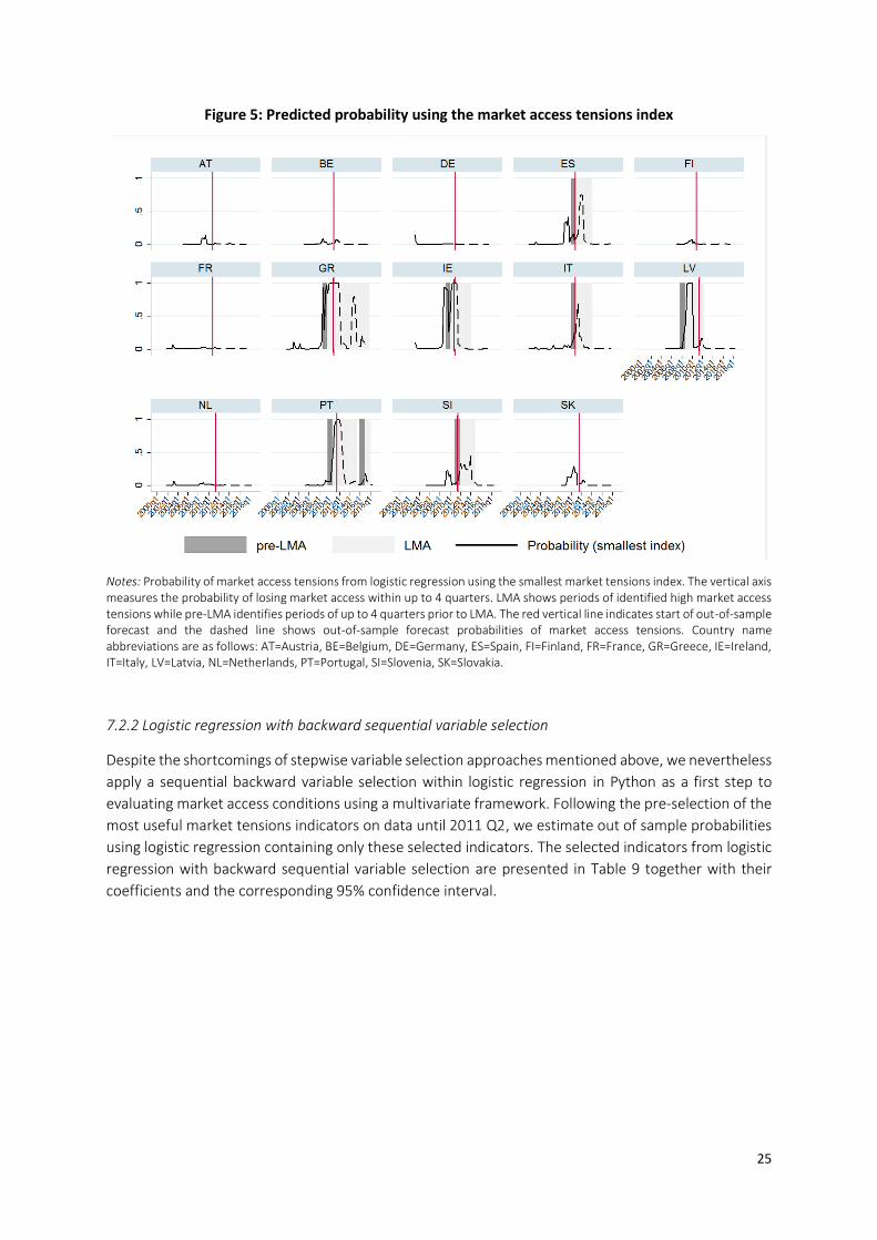
25
Figure 5: Predicted probability using the market access tensions index
Notes: Probability of market access tensions from logistic regression using the smallest market tensions index. The vertical axis measures the probability of losing market access within up to 4 quarters. LMA shows periods of identified high market access tensions while pre-LMA identifies periods of up to 4 quarters prior to LMA. The red vertical line indicates start of out-of-sample forecast and the dashed line shows out-of-sample forecast probabilities of market access tensions. Country name abbreviations are as follows: AT=Austria, BE=Belgium, DE=Germany, ES=Spain, FI=Finland, FR=France, GR=Greece, IE=Ireland, IT=Italy, LV=Latvia, NL=Netherlands, PT=Portugal, SI=Slovenia, SK=Slovakia.
7.2.2 Logistic regression with backward sequential variable selection
Despite the shortcomings of stepwise variable selection approaches mentioned above, we nevertheless
apply a sequential backward variable selection within logistic regression in Python as a first step to
evaluating market access conditions using a multivariate framework. Following the pre-selection of the
most useful market tensions indicators on data until 2011 Q2, we estimate out of sample probabilities
using logistic regression containing only these selected indicators. The selected indicators from logistic
regression with backward sequential variable selection are presented in Table 9 together with their
coefficients and the corresponding 95% confidence interval.
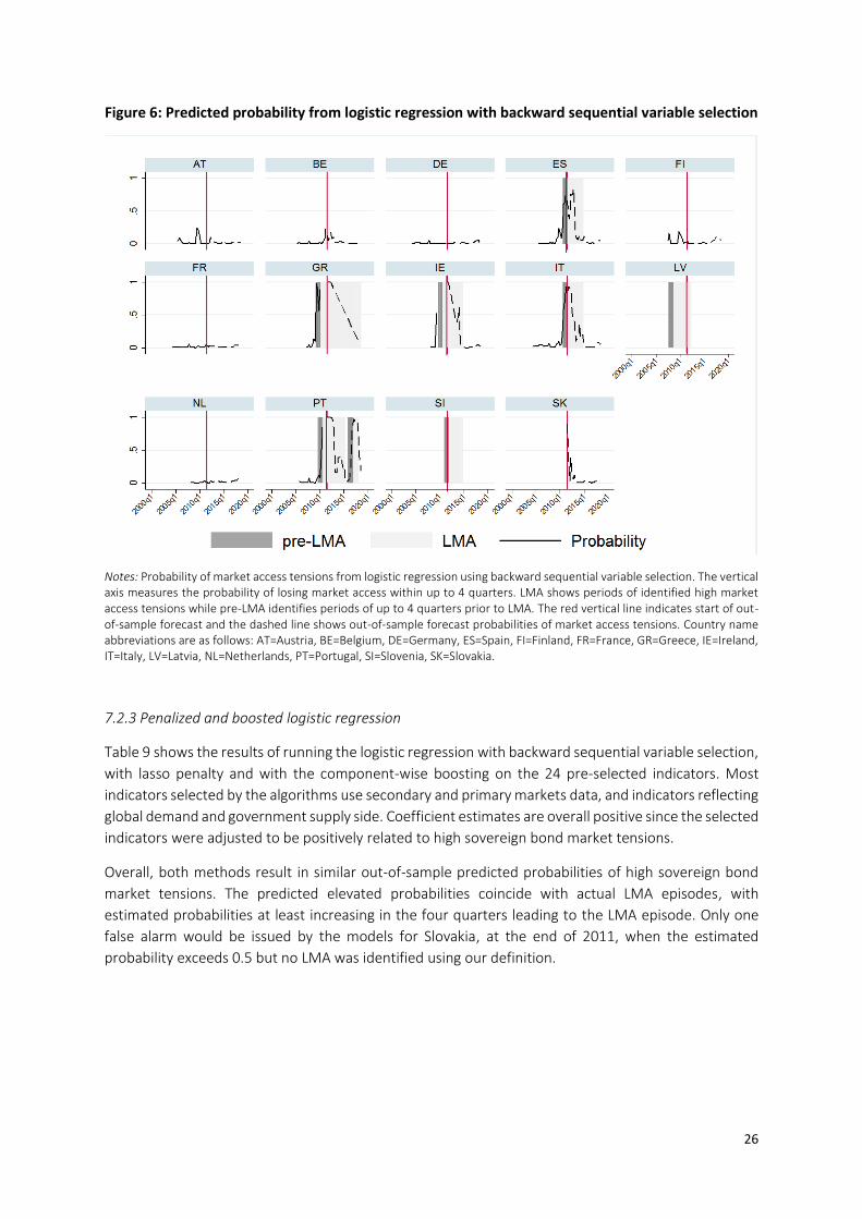
26
Figure 6: Predicted probability from logistic regression with backward sequential variable selection
Notes: Probability of market access tensions from logistic regression using backward sequential variable selection. The vertical axis measures the probability of losing market access within up to 4 quarters. LMA shows periods of identified high market access tensions while pre-LMA identifies periods of up to 4 quarters prior to LMA. The red vertical line indicates start of out-of-sample forecast and the dashed line shows out-of-sample forecast probabilities of market access tensions. Country name abbreviations are as follows: AT=Austria, BE=Belgium, DE=Germany, ES=Spain, FI=Finland, FR=France, GR=Greece, IE=Ireland, IT=Italy, LV=Latvia, NL=Netherlands, PT=Portugal, SI=Slovenia, SK=Slovakia.
7.2.3 Penalized and boosted logistic regression
Table 9 shows the results of running the logistic regression with backward sequential variable selection,
with lasso penalty and with the component-wise boosting on the 24 pre-selected indicators. Most
indicators selected by the algorithms use secondary and primary markets data, and indicators reflecting
global demand and government supply side. Coefficient estimates are overall positive since the selected
indicators were adjusted to be positively related to high sovereign bond market tensions.
Overall, both methods result in similar out-of-sample predicted probabilities of high sovereign bond
market tensions. The predicted elevated probabilities coincide with actual LMA episodes, with
estimated probabilities at least increasing in the four quarters leading to the LMA episode. Only one
false alarm would be issued by the models for Slovakia, at the end of 2011, when the estimated
probability exceeds 0.5 but no LMA was identified using our definition.
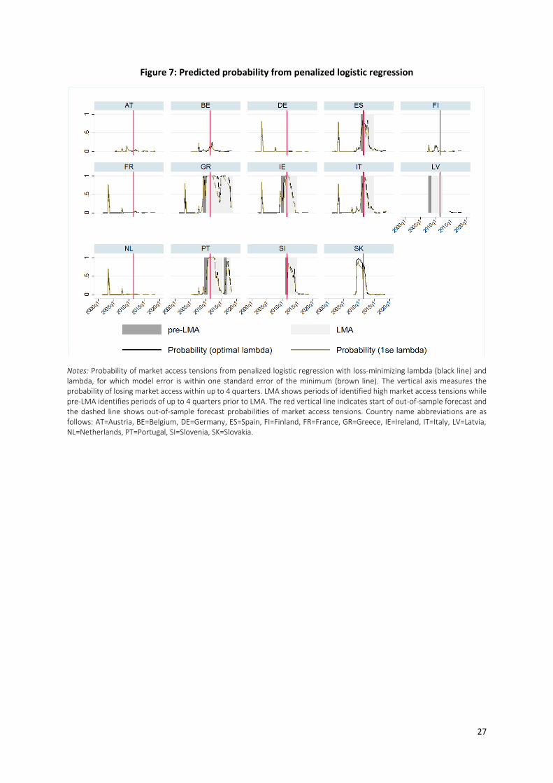
27
Figure 7: Predicted probability from penalized logistic regression
Notes: Probability of market access tensions from penalized logistic regression with loss-minimizing lambda (black line) and lambda, for which model error is within one standard error of the minimum (brown line). The vertical axis measures the probability of losing market access within up to 4 quarters. LMA shows periods of identified high market access tensions while pre-LMA identifies periods of up to 4 quarters prior to LMA. The red vertical line indicates start of out-of-sample forecast and the dashed line shows out-of-sample forecast probabilities of market access tensions. Country name abbreviations are as follows: AT=Austria, BE=Belgium, DE=Germany, ES=Spain, FI=Finland, FR=France, GR=Greece, IE=Ireland, IT=Italy, LV=Latvia, NL=Netherlands, PT=Portugal, SI=Slovenia, SK=Slovakia.
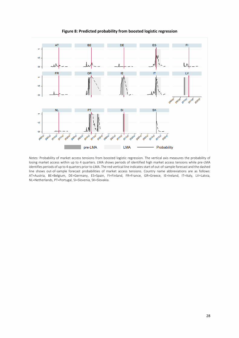
28
Figure 8: Predicted probability from boosted logistic regression
Notes: Probability of market access tensions from boosted logistic regression. The vertical axis measures the probability of losing market access within up to 4 quarters. LMA shows periods of identified high market access tensions while pre-LMA identifies periods of up to 4 quarters prior to LMA. The red vertical line indicates start of out-of-sample forecast and the dashed line shows out-of-sample forecast probabilities of market access tensions. Country name abbreviations are as follows: AT=Austria, BE=Belgium, DE=Germany, ES=Spain, FI=Finland, FR=France, GR=Greece, IE=Ireland, IT=Italy, LV=Latvia, NL=Netherlands, PT=Portugal, SI=Slovenia, SK=Slovakia.
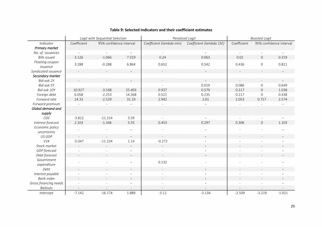
29
Table 9: Selected Indicators and their coefficient estimates
Logit with Sequential Selection Penalized Logit Boosted Logit
Indicator Coefficient 95% confidence interval Coefficient (lambda min) Coefficient (lambda 1SE) Coefficient 95% confidence interval Primary market
No. of issuances - - - - - - - -
Bills issued 3.126 -1.066 7.319 0.24 0.063 0.02 0 0.319 Floating coupon
issuance 3.288 -0.288 6.864 0.652 0.542 0.436 0 0.811
Syndicated issuance - - - - - - - -
Secondary market
Bid-ask 2Y - - - - - - - -
Bid-ask 5Y - 0.019 0.086 0 0.649 Bid-ask 10Y 10.927 -3.548 25.403 0.937 0.579 0.317 0 1.038
Foreign debt 6.058 -2.253 14.368 0.521 0.235 0.217 0 0.438 Forward rate 14.33 -2.529 31.19 2.942 2.61 2.053 0.757 2.574
Forward premium - - - - - - - -
Global demand and supply
CDS -3.812 -11.214 3.59 - - - - -
Interest forecast 2.103 -1.346 5.55 0.453 0.297 0.306 0 1.103 Economic policy
uncertainty - - - - - - - -
US GDP - - - - - - - -
V2X -5.047 -11.234 1.14 -0.272 - - - -
Stock market - - - - - - - -
GDP forecast - - - - - - - -
Debt forecast - - - - - - - -
Government expenditure
- - - 0.132 - - - -
Debt - - - - - - - -
Interest payable - - - - - - - -
Bank index - - - - - - - -
Gross financing needs - - - - - - - -
Bailouts - - - - - - - -
Intercept -7.142 -16.174 1.889 -3.12 -3.134 -2.509 -3.219 -1.921
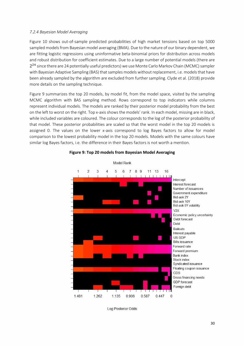
30
7.2.4 Bayesian Model Averaging
Figure 10 shows out-of-sample predicted probabilities of high market tensions based on top 5000
sampled models from Bayesian model averaging (BMA). Due to the nature of our binary dependent, we
are fitting logistic regressions using uninformative beta-binomial priors for distribution across models
and robust distribution for coefficient estimates. Due to a large number of potential models (there are
224 since there are 24 potentially useful predictors) we use Monte Carlo Markov Chain (MCMC) sampler
with Bayesian Adaptive Sampling (BAS) that samples models without replacement, i.e. models that have
been already sampled by the algorithm are excluded from further sampling. Clyde et al. (2018) provide
more details on the sampling technique.
Figure 9 summarizes the top 20 models, by model fit, from the model space, visited by the sampling
MCMC algorithm with BAS sampling method. Rows correspond to top indicators while columns
represent individual models. The models are ranked by their posterior model probability from the best
on the left to worst on the right. Top x-axis shows the models’ rank. In each model, missing are in black,
while included variables are coloured. The colour corresponds to the log of the posterior probability of
that model. These posterior probabilities are scaled so that the worst model in the top 20 models is
assigned 0. The values on the lower x-axis correspond to log Bayes factors to allow for model
comparison to the lowest probability model in the top 20 models. Models with the same colours have
similar log Bayes factors, i.e. the difference in their Bayes factors is not worth a mention.
Figure 9: Top 20 models from Bayesian Model Averaging
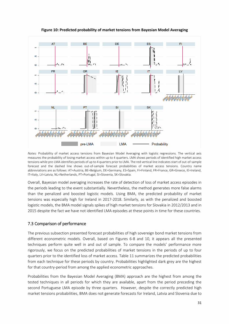
31
Figure 10: Predicted probability of market tensions from Bayesian Model Averaging
Notes: Probability of market access tensions from Bayesian Model Averaging with logistic regressions. The vertical axis measures the probability of losing market access within up to 4 quarters. LMA shows periods of identified high market access tensions while pre-LMA identifies periods of up to 4 quarters prior to LMA. The red vertical line indicates start of out-of-sample forecast and the dashed line shows out-of-sample forecast probabilities of market access tensions. Country name abbreviations are as follows: AT=Austria, BE=Belgium, DE=Germany, ES=Spain, FI=Finland, FR=France, GR=Greece, IE=Ireland, IT=Italy, LV=Latvia, NL=Netherlands, PT=Portugal, SI=Slovenia, SK=Slovakia.
Overall, Bayesian model averaging increases the rate of detection of loss of market access episodes in
the periods leading to the event substantially. Nevertheless, the method generates more false alarms
than the penalized and boosted logistic models. Using BMA, the predicted probability of market
tensions was especially high for Ireland in 2017-2018. Similarly, as with the penalized and boosted
logistic models, the BMA model signals spikes of high market tensions for Slovakia in 2012/2013 and in
2015 despite the fact we have not identified LMA episodes at these points in time for these countries.
7.3 Comparison of performance
The previous subsection presented forecast probabilities of high sovereign bond market tensions from
different econometric models. Overall, based on Figures 6-8 and 10, it appears all the presented
techniques perform quite well in and out of sample. To compare the models’ performance more
rigorously, we focus on the predicted probabilities of market tensions in the periods of up to four
quarters prior to the identified loss of market access. Table 11 summarizes the predicted probabilities
from each technique for these periods by country. Probabilities highlighted dark grey are the highest
for that country-period from among the applied econometric approaches.
Probabilities from the Bayesian Model Averaging (BMA) approach are the highest from among the
tested techniques in all periods for which they are available, apart from the period preceding the
second Portuguese LMA episode by three quarters. However, despite the correctly predicted high
market tensions probabilities, BMA does not generate forecasts for Ireland, Latvia and Slovenia due to
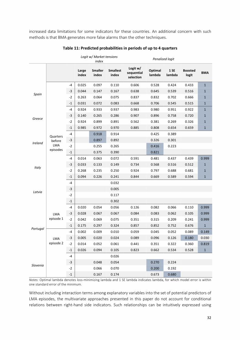
32
increased data limitations for some indicators for these countries. An additional concern with such
methods is that BMA generates more false alarms than the other techniques.
Table 11: Predicted probabilities in periods of up to 4 quarters
Logit w/ Market tensions index
Penalized logit
Large index
Smaller index
Smallest index
Logit w/ sequential selection
Optimal lambda
1 SE lambda
Boosted logit
BMA
Spain
Quarters before LMA
episodes
-4 0.025 0.097 0.110 0.606 0.528 0.424 0.433 1
-3 0.044 0.147 0.167 0.638 0.645 0.539 0.516 1
-2 0.263 0.064 0.075 0.837 0.832 0.702 0.666 1
-1 0.031 0.072 0.083 0.668 0.706 0.545 0.515 1
Greece
-4 0.924 0.933 0.937 0.983 0.980 0.951 0.922 1
-3 0.140 0.265 0.286 0.907 0.896 0.758 0.720 1
-2 0.924 0.899 0.891 0.562 0.381 0.269 0.326 1
-1 0.985 0.972 0.970 0.885 0.808 0.654 0.659 1
Ireland
-4 0.918 0.914 0.425 0.389
-3 0.897 0.892 0.326 0.301
-2 0.255 0.265 0.416 0.223
-1 0.375 0.390 0.821
Italy
-4 0.014 0.063 0.072 0.591 0.481 0.437 0.439 0.999
-3 0.033 0.133 0.149 0.734 0.568 0.516 0.512 1
-2 0.268 0.235 0.250 0.924 0.797 0.688 0.681 1
-1 0.094 0.226 0.241 0.844 0.669 0.589 0.594 1
Latvia
-4 0.032
-3 0.005
-2 0.117
-1 0.302
Portugal
LMA episode 1
-4 0.020 0.054 0.056 0.126 0.082 0.066 0.110 0.999
-3 0.028 0.067 0.067 0.084 0.083 0.062 0.105 0.999
-2 0.042 0.069 0.075 0.351 0.315 0.209 0.241 0.999
-1 0.175 0.297 0.324 0.857 0.852 0.752 0.676 1
LMA episode 2
-4 0.002 0.009 0.010 0.059 0.045 0.052 0.089 0.149
-3 0.005 0.020 0.024 0.089 0.096 0.126 0.180 0.030
-2 0.014 0.052 0.061 0.441 0.351 0.322 0.360 0.819
-1 0.026 0.094 0.105 0.823 0.662 0.534 0.528 1
Slovenia
-4 0.026
-3 0.048 0.054 0.270 0.224
-2 0.066 0.070 0.200 0.192
-1 0.167 0.174 0.673 0.680
Notes: Optimal lambda denotes loss-minimizing lambda and 1 SE lambda indicates lambda, for which model error is within one standard error of the minimum.
Without including interaction terms among explanatory variables into the set of potential predictors of
LMA episodes, the multivariate approaches presented in this paper do not account for conditional
relations between right-hand side indicators. Such relationships can be intuitively expressed using
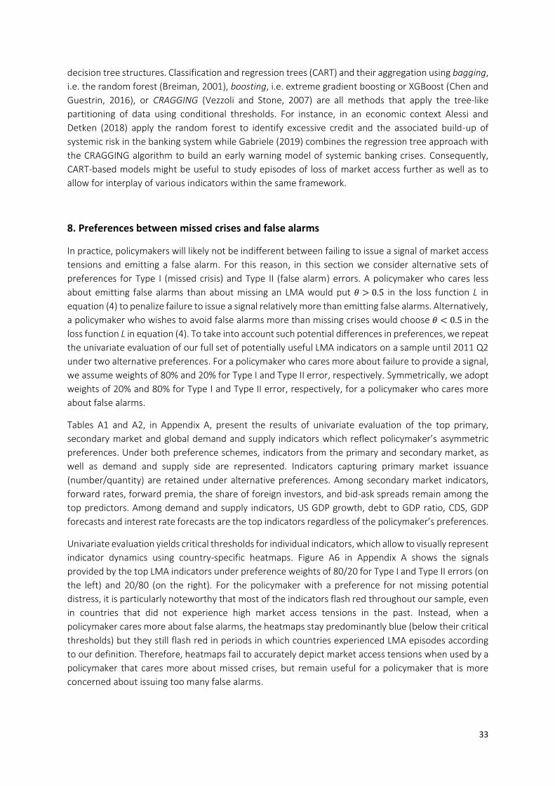
33
decision tree structures. Classification and regression trees (CART) and their aggregation using bagging,
i.e. the random forest (Breiman, 2001), boosting, i.e. extreme gradient boosting or XGBoost (Chen and
Guestrin, 2016), or CRAGGING (Vezzoli and Stone, 2007) are all methods that apply the tree-like
partitioning of data using conditional thresholds. For instance, in an economic context Alessi and
Detken (2018) apply the random forest to identify excessive credit and the associated build-up of
systemic risk in the banking system while Gabriele (2019) combines the regression tree approach with
the CRAGGING algorithm to build an early warning model of systemic banking crises. Consequently,
CART-based models might be useful to study episodes of loss of market access further as well as to
allow for interplay of various indicators within the same framework.
8. Preferences between missed crises and false alarms
In practice, policymakers will likely not be indifferent between failing to issue a signal of market access
tensions and emitting a false alarm. For this reason, in this section we consider alternative sets of
preferences for Type I (missed crisis) and Type II (false alarm) errors. A policymaker who cares less
about emitting false alarms than about missing an LMA would put 𝜃 > 0.5 in the loss function L in
equation (4) to penalize failure to issue a signal relatively more than emitting false alarms. Alternatively,
a policymaker who wishes to avoid false alarms more than missing crises would choose 𝜃 < 0.5 in the
loss function L in equation (4). To take into account such potential differences in preferences, we repeat
the univariate evaluation of our full set of potentially useful LMA indicators on a sample until 2011 Q2
under two alternative preferences. For a policymaker who cares more about failure to provide a signal,
we assume weights of 80% and 20% for Type I and Type II error, respectively. Symmetrically, we adopt
weights of 20% and 80% for Type I and Type II error, respectively, for a policymaker who cares more
about false alarms.
Tables A1 and A2, in Appendix A, present the results of univariate evaluation of the top primary,
secondary market and global demand and supply indicators which reflect policymaker’s asymmetric
preferences. Under both preference schemes, indicators from the primary and secondary market, as
well as demand and supply side are represented. Indicators capturing primary market issuance
(number/quantity) are retained under alternative preferences. Among secondary market indicators,
forward rates, forward premia, the share of foreign investors, and bid-ask spreads remain among the
top predictors. Among demand and supply indicators, US GDP growth, debt to GDP ratio, CDS, GDP
forecasts and interest rate forecasts are the top indicators regardless of the policymaker’s preferences.
Univariate evaluation yields critical thresholds for individual indicators, which allow to visually represent
indicator dynamics using country-specific heatmaps. Figure A6 in Appendix A shows the signals
provided by the top LMA indicators under preference weights of 80/20 for Type I and Type II errors (on
the left) and 20/80 (on the right). For the policymaker with a preference for not missing potential
distress, it is particularly noteworthy that most of the indicators flash red throughout our sample, even
in countries that did not experience high market access tensions in the past. Instead, when a
policymaker cares more about false alarms, the heatmaps stay predominantly blue (below their critical
thresholds) but they still flash red in periods in which countries experienced LMA episodes according
to our definition. Therefore, heatmaps fail to accurately depict market access tensions when used by a
policymaker that cares more about missed crises, but remain useful for a policymaker that is more
concerned about issuing too many false alarms.
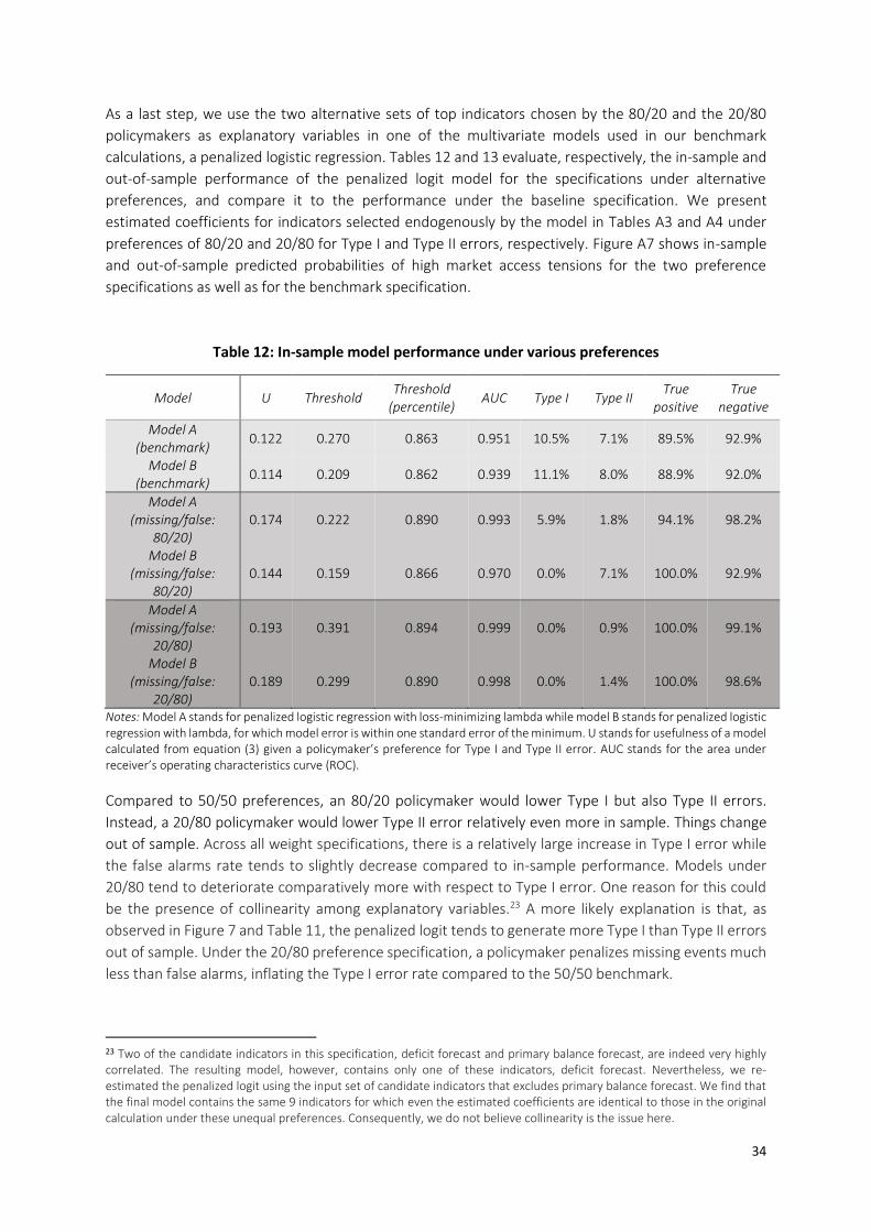
34
As a last step, we use the two alternative sets of top indicators chosen by the 80/20 and the 20/80
policymakers as explanatory variables in one of the multivariate models used in our benchmark
calculations, a penalized logistic regression. Tables 12 and 13 evaluate, respectively, the in-sample and
out-of-sample performance of the penalized logit model for the specifications under alternative
preferences, and compare it to the performance under the baseline specification. We present
estimated coefficients for indicators selected endogenously by the model in Tables A3 and A4 under
preferences of 80/20 and 20/80 for Type I and Type II errors, respectively. Figure A7 shows in-sample
and out-of-sample predicted probabilities of high market access tensions for the two preference
specifications as well as for the benchmark specification.
Table 12: In-sample model performance under various preferences
Model U Threshold Threshold
(percentile) AUC Type I Type II
True positive
True negative
Model A (benchmark)
0.122 0.270 0.863 0.951 10.5% 7.1% 89.5% 92.9%
Model B (benchmark)
0.114 0.209 0.862 0.939 11.1% 8.0% 88.9% 92.0%
Model A (missing/false:
80/20) 0.174 0.222 0.890 0.993 5.9% 1.8% 94.1% 98.2%
Model B (missing/false:
80/20) 0.144 0.159 0.866 0.970 0.0% 7.1% 100.0% 92.9%
Model A (missing/false:
20/80) 0.193 0.391 0.894 0.999 0.0% 0.9% 100.0% 99.1%
Model B (missing/false:
20/80) 0.189 0.299 0.890 0.998 0.0% 1.4% 100.0% 98.6%
Notes: Model A stands for penalized logistic regression with loss-minimizing lambda while model B stands for penalized logistic regression with lambda, for which model error is within one standard error of the minimum. U stands for usefulness of a model calculated from equation (3) given a policymaker’s preference for Type I and Type II error. AUC stands for the area under receiver’s operating characteristics curve (ROC).
Compared to 50/50 preferences, an 80/20 policymaker would lower Type I but also Type II errors.
Instead, a 20/80 policymaker would lower Type II error relatively even more in sample. Things change
out of sample. Across all weight specifications, there is a relatively large increase in Type I error while
the false alarms rate tends to slightly decrease compared to in-sample performance. Models under
20/80 tend to deteriorate comparatively more with respect to Type I error. One reason for this could
be the presence of collinearity among explanatory variables.23 A more likely explanation is that, as
observed in Figure 7 and Table 11, the penalized logit tends to generate more Type I than Type II errors
out of sample. Under the 20/80 preference specification, a policymaker penalizes missing events much
less than false alarms, inflating the Type I error rate compared to the 50/50 benchmark.
23 Two of the candidate indicators in this specification, deficit forecast and primary balance forecast, are indeed very highly correlated. The resulting model, however, contains only one of these indicators, deficit forecast. Nevertheless, we re-estimated the penalized logit using the input set of candidate indicators that excludes primary balance forecast. We find that the final model contains the same 9 indicators for which even the estimated coefficients are identical to those in the original calculation under these unequal preferences. Consequently, we do not believe collinearity is the issue here.
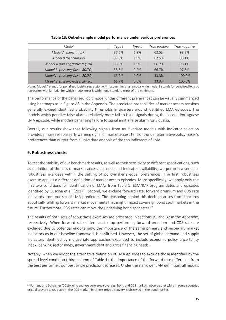
35
Table 13: Out-of-sample model performance under various preferences
Model Type I Type II True positive True negative
Model A (benchmark) 37.5% 1.8% 62.5% 98.2%
Model B (benchmark) 37.5% 1.9% 62.5% 98.1%
Model A (missing/false: 80/20) 33.3% 1.9% 66.7% 98.1%
Model B (missing/false: 80/20) 33.3% 2.2% 66.7% 97.8%
Model A (missing/false: 20/80) 66.7% 0.0% 33.3% 100.0%
Model B (missing/false: 20/80) 66.7% 0.0% 33.3% 100.0%
Notes: Model A stands for penalized logistic regression with loss-minimizing lambda while model B stands for penalized logistic regression with lambda, for which model error is within one standard error of the minimum.
The performance of the penalized logit model under different preferences can be visually summarized
using heatmaps as in Figure A8 in the Appendix. The predicted probabilities of market access tensions
generally exceed identified probability thresholds in quarters around identified LMA episodes. The
models which penalize false alarms relatively more fail to issue signals during the second Portuguese
LMA episode, while models penalizing failure to signal emit a false alarm for Slovakia.
Overall, our results show that following signals from multivariate models with indicator selection
provides a more reliable early warning signal of market access tensions under alternative policymaker’s
preferences than output from a univariate analysis of the top indicators of LMA.
9. Robustness checks
To test the stability of our benchmark results, as well as their sensitivity to different specifications, such
as definition of the loss of market access episodes and indicator availability, we perform a series of
robustness exercises within the setting of policymaker’s equal preferences. The first robustness
exercise applies a different definition of market access episodes. More specifically, we apply only the
first two conditions for identification of LMAs from Table 1: ESM/IMF program dates and episodes
identified by Guscina et al. (2017). Second, we exclude forward rate, forward premium and CDS rate
indicators from our set of LMA predictors. The reasoning behind this decision arises from concerns
about self-fulfilling forward market movements that might impact sovereign bond spot markets in the
future. Furthermore, CDS rates can move the underlying bond spot rates.24
The results of both sets of robustness exercises are presented in sections B1 and B2 in the Appendix,
respectively. When forward rate difference to top performer, forward premium and CDS rate are
excluded due to potential endogeneity, the importance of the same primary and secondary market
indicators as in our baseline framework is confirmed. However, the set of global demand and supply
indicators identified by multivariate approaches expanded to include economic policy uncertainty
index, banking sector index, government debt and gross financing needs.
Notably, when we adopt the alternative definition of LMA episodes to exclude those identified by the
spread level condition (third column of Table 1), the importance of the forward rate difference from
the best performer, our best single predictor decreases. Under this narrower LMA definition, all models
24 Fontana and Scheicher (2016), who analyse euro area sovereign bond and CDS markets, observe that while in some countries price discovery takes place in the CDS market, in others price discovery is observed in the bond market.
36
still report small to moderate increases in market access distress probabilities in late 2011/2012 for
Italy.25
Conclusions
In this paper we study episodes of sovereign loss of market access. We construct a detailed dataset
with potential indicators of market access tensions, as identified by market experts and the academic
literature, and evaluate their ability to forecast market access tensions.
Univariate analysis shows that factors associated with high market access tensions are not limited to
financial markets, but encompass also developments in global demand, macroeconomic factors and
the fiscal stance. Forward rate difference from the best performer emerged as the most important
predictor of market access tensions. The identified informative indicators of market access tensions
are, however, too numerous to be meaningfully included within a multivariate model that generalizes
well out of sample. To select which variables should be included in the final model, we apply several
approaches to resolving model uncertainty; we construct a market tensions index (MTI) to use as a
single predictor; we sequentially eliminate variables one by one from conventional logit model; and we
estimate lasso and boosted logit models. Lastly, we run logit models using many combinations of the
top identified LMA indicators and report the weighted results from the model space. We find that the
more complex methods outperform predicted probabilities from simple logit with MTI, which are
generally quite low in the quarters preceding LMA outbreaks. The most complex method, BMA, yields
the highest probabilities of LMA in the quarters leading to the LMA incidence across countries included
in our panel. In contrast, BMA also generates more false alarms than the other methods.
We consider two scenarios when a policymaker is not indifferent between missing an LMA episode and
issuing a false alarm. In one scenario, a policymaker cares more about missing an LMA event. In the
other, she is more concerned about issuing false alarms. Regardless of the policymaker’s preference,
the number and quantity of primary market issuance, forward rates, forward premia, bid-ask spreads,
the share of foreign investors, US GDP growth, debt to GDP ratio, CDS, GDP forecasts and interest rate
forecasts are among the top indicators of market access tensions. We further show that a policymaker
who cares more about missing an LMA episode would not be able to provide an appropriate policy
response based on univariate signals from individual indicators which flash red over most periods in our
sample, even in countries that did not experience high market access tensions. Instead, signals from a
univariate analysis would still be useful and flash red in periods in which countries experienced an LMA
episode if the policymaker is more concerned about issuing false alarms. In a multivariate setting,
models with indicator selection provide a more reliable early warning signal of market access tensions
than individual indicators separately under both types of policymaker’s asymmetric preferences.
Our results point to a trade-off between transparency/communicability and accuracy that policymakers
face in the search for tools to evaluate risks to market access. While transparent and easy to
communicate, single indices of market tensions can capture worsening conditions in accessing
financing from bond markets but do not typically yield satisfactory out-of-sample results. Conversely,
multivariate models perform better, but are harder to explain in a simple and transparent way.
25 The spike in the projected probability of tensions in the Italian bond market represents, in a strict sense, a false alarm. One
could, however, link this increase in predicted market tensions to another policy reaction, which reportedly aimed at reducing tensions in sovereign bond markets, because they were hampering the transmission of monetary policy - Draghi’s “Whatever it takes” speech.
37
References
Abbas, A., Blattner, L., De Broeck, M., El-Ganainy, A., & Hu, M., 2014. “Sovereign Debt Composition in
Advanced Economies: A Historical Perspective”. IMF Working Papers 14/162.
Alesina, A., De Broeck, M., Prati, A. & Tabellini, G., 1992. “Default risk on government debt in OECD
countries”. Economic Policy, vol. 15, pp. 427-451.
Alessi, L. & Detken, C., 2011. "Quasi real time early warning indicators for costly asset price boom/bust
cycles: A role for global liquidity". European Journal of Political Economy, vol. 27(3), pp 520-533.
Alessi,L. & Detken, C., 2018. “Identifying excessive credit growth and leverage”. Journal of Financial
Stability, vol. 35, pp. 215-225.
Arellano, C., & Ramanarayanan, A., 2012. “Default and the Maturity Structure in Sovereign Bonds”.
Journal of Political Economy, vol. 120(2), pp. 187-232.
Ariccia, G., Ferreira, C., Jenkinson, N., Laeven, L., Martin, A., Minoiu, C., & Popov. A, 2018. “Managing
the sovereign-bank nexus”. ECB Working Paper no. 2177.
Arslanalp, S., & Poghosyan, T., 2014. “Foreign Investor Flows and Sovereign Bond Yields in Advanced
Economies”. IMF Working Papers 14/27.
Arslanalp, S., & Liao, Y., 2014. “Banking sector contingent liabilities and sovereign risk”. Journal of
Empirical Finance, vol. 29, pp. 316-330.
Baker, S., Bloom, N., & Davis, S., 2016. “Measuring Economic Policy Uncertainty”. The Quarterly Journal
of Economics, vol. 131(4), pp. 1593–1636.
Baldacci, E., Petrova, I. K., Belhocine, N., Dobrescu, G. & Mazraani, S., 2011. “Assessing Fiscal Stress”.
IMF Working Papers 11/100.
Baldacci, E., McHugh, J., & Petrova, I., 2011. “Measuring Fiscal Vulnerability and Fiscal Stress: A
Proposed Set of Indicators”. IMF Working Paper 11/94.
Balteanu, I., & Erce, A., 2017. “Linking Bank Crises and Sovereign Defaults: Evidence from Emerging
Markets”. ESM Working Paper, 22/2017.
Bassanetti, A., Cottarelli, C., & A. Presbitero, 2016. “Lost and Found: Market Access and Public Debt
Dynamics. IMF Working Paper 16/253.
Baur, D., & Lucey, B., 2009. “Flights and contagion— An empirical analysis of stock– bond correlations”.
Journal of Financial Stability, vol. 5(4), pp. 339-352.
Belton, T., Dawsey, K., Greenlaw, D., Huacen, L., Ramaswamy, S., & B. Sack, 2018. “Optimizing the
Maturity Structure of US Treasury Debt: A Model-Based Framework,” Hutchins Centre, Working Paper
No. 46.
Beetsma, R., Giuliodori, M., Hanson, J. & De Jong, F., 2018. “Cross-border auction cycle effects of
sovereign bond issuance in the Euro Area”. Journal of Money, Credit and Banking, forthcoming.
Beetsma, R., Giuliodori, M., Hanson, J. & De Jong, F., 2018. “Bid-to-cover and yield changes around
public debt auctions in the euro area”. Journal of Banking & Finance, 87, pp. 118-134.
Bernoth, K., von Hagen, J., Schuknecht, L., 2004. “Sovereign risk premia in the European government
bond market”. ECB Working Paper 369.

38
Bordo, M., & Haubrich, J., 2008. “The yield curve as a predictor of growth: Long-run evidence 1875-
1997”. Review of Economics and Statistics, vol. 90, pp. 182-185.
Breiman, L. (2001): “Random forests.” Machine Learning 45 (1), pp. 5–32.
Broner, F.A., Lorenzoni, G. & Schmukler, S.L., 2013. “Why do emerging economies borrow short term?”
Journal of the European Economic Association, Vol.11 (S1), pp. 67-100.
Buhlmann, P., 2006. “Boosting for high-dimensional linear models”. The Annals of Statistics, vol. 34, pp.
559–583.
Buhlmann, P. & Yu, B., 2003. “Boosting with the L2 loss: Regression and classification”. Journal of the
American Statistical Association, vol. 98, pp. 324–338.
Bussiere, M. & Fratzscher, M., 2006. "Towards a new early warning system of financial crises," Journal
of International Money and Finance, Elsevier, vol. 25(6), pp. 953-973, October.
Candelon, B., Dumitrescu E. & Hurlin, C., 2012. "How to Evaluate an Early-Warning System: Toward a
Unified Statistical Framework for Assessing Financial Crises Forecasting Methods". IMF Economic
Review, vol. 60(1), pp. 75-113.
Casalinho, C., Kalozois, P., O´Connor, F., de Ramon-Laca, P., Rojas, J., & R. Strauch, 2016. “Accessing
sovereign markets – the recent experiences of Ireland, Portugal, Spain and Cyprus”, ESM Discussion
Paper Series No.2.
Chen, T. & Guestrin, C., 2016. “XGBoost: A Scalable Tree Boosting System”. Proceedings of the 22nd
ACM SIGKDD International Conference on Knowledge Discovery and Data Mining, San Francisco,
California, USA, pp. 785-794.
Clyde, M., Littman, M., Wang, Q., Ghosh, J. & Li, Y., 2018. “Bayesian Variable Selection and Model
Averaging using Bayesian Adaptive Sampling”, mimeo.
Cruz, P., & Koc, F., 2018. "The liquidity buffer practices of public debt managers in OECD countries".
OECD Working Papers on Sovereign Borrowing and Public Debt Management, No. 9, OECD.
De Broeck, M., & Guscina, A., 2011. “Government Debt Issuance in the Euro Area: The Impact of the
Financial Crisis”, IMF Working Paper 11/21.
Engle, R., & J. Rangel, 2008. “The spline GARCH model for low frequency volatility and its global
macroeconomic causes”. The Review of Financial Studies, vol. 21(3), pp. 1187-1222.
Estrella, A., & Hardouvelis, G., 1991. “The Term Structure as a Predictor of Real Economic Activity”. The
Journal of Finance, Vol. 46, No. 2, pp. 555-576.
Estrella, A., & Mishkin, F., 1998. “Predicting U.S. Recessions: Financial Variables as Leading Indicators”.
The Review of Economics and Statistics, Vol, 80, pp. 45-61.
Eidam, F., 2017. “Gap-Filling Government Debt Maturity Choice,” ZEW Discussion Papers 18-025.
Gabriele, C., 2019. “Learning from Trees: A Mixed Approach to Building Early Warning Systems for
Systemic Banking Crises”. ESM Working Paper 40/2019.
Gabriele, C., Erce, A., Athanasopoulou, M., & Rojas, J., 2017. “Debt Stocks Meet Gross Financing Needs:
A Flow Perspective into Sustainability”. ESM Working Paper 24/2017.
Gelper, S., & Croux, C., 2010. “On the Construction of the European Economic Sentiment
Indicator”. Oxford Bulletin of Economics and Statistics, vol. 72(1), pp. 47-62.

39
P.R. Fisher, 2012. “Thoughts on Debt Sustainability: Supply and Demand,” keynote remarks published
in Is U.S. Government Debt Different?” Wharton Financial Institutions Centre Press.
Fontana, A., & Scheicher, M., 2016. “An analysis of euro area sovereign CDS and their relation with
government bonds”. Journal of Banking & Finance, Volume 62, pp. 126-140,
Friedman, J., Hastie, T. & Tibshirani, R., 2008. “Regularization Paths for Generalized Linear Models via
Coordinate Descent”, available at: https://web.stanford.edu/~hastie/Papers/glmnet.pdf
Gelos, G., Sahay, R., & G. Sandleris, 2004. “Sovereign Borrowing by Developing Economies: What
Determines Market Access?” IMF Working Paper 04/221.
Gerlach, S., & Stuart, R., 2018. “The Slope of the Term Structure and Recessions: The Pre-Fed Evidence,
1857-1913”. CEPR Discussion Paper No. DP13013.
Guscina, A., Malik, S. & Papaioannou, M., 2017. "Assessing Loss of Market Access: Conceptual and
Operational Issues". IMF Working Papers 17/246.
Hastie, T., Tibshirani, R. & Friedman, J., 2009. “The Elements of Statistical Learning: Data Mining,
Inference, and Prediction”. Springer, New York.
Hauner, D. & Kumar, M., 2006. “Fiscal Policy and Interest Rates--How Sustainable Is the New Economy?”
IMF Working Paper No. 06/112.
Jaramilllo, L., & Zhang, Y., 2013. “Real Money Investors and Sovereign Bond Yields”. IMF Working
Papers 13/254.
Jonasson, T., & Papaioannou, M., 2018. “Sovereign Debt Management During Debt Distress Periods”
Journal of Investing, Vol. 27, Issue 3, pp. 65-73.
Jonasson, T., & Papaioannou, M., 2018. “A primer on managing sovereign debt-portfolio risks”. IMF
Working Paper 18/74.
Koop, G., 2003. “Bayesian Econometrics”. John Wiley & Sons.
Lang, J. H., Izzo, C., Fahr, S., & Ruzicka, J., 2019. “Anticipating the bust: a new cyclical systemic risk
indicator to assess the likelihood and severity of financial crises”, ECB Occasional Paper Series No. 219.
Roecker, E. B., 1991. “Prediction error and its estimation for subset - selected models”. Technometrics,
vol. 33, pp. 459–468.
Schalck, C., 2017. “Public Debt Management in Developed Economies During the Crisis”, Global
Financial Crisis and Its Ramifications on Capital Markets, Contributions to Economics (Haciogllu &
Dincer).
Sigaux, J.D., 2018.” Trading ahead of Treasury auctions”, ECB Working Paper Series No. 2208.
Vezzoli, M. and C. Stone, 2007. “Cragging”, manuscript, Department of Statistics, University of
California, Berkeley.
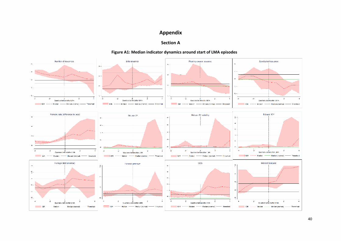
40
Appendix
Section A
Figure A1: Median indicator dynamics around start of LMA episodes
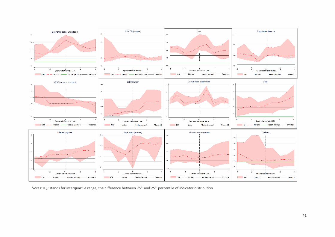
41
Notes: IQR stands for interquartile range; the difference between 75th and 25th percentile of indicator distribution
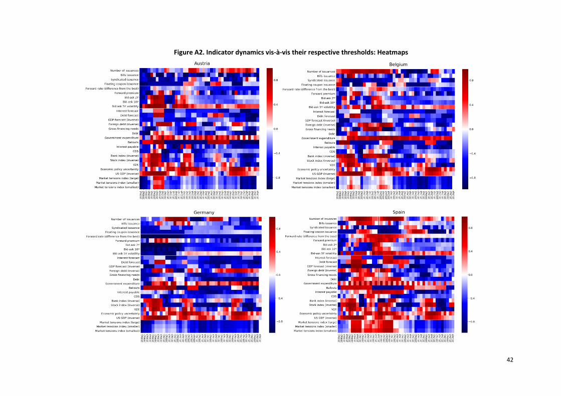
42
Figure A2. Indicator dynamics vis-à-vis their respective thresholds: Heatmaps

43

44
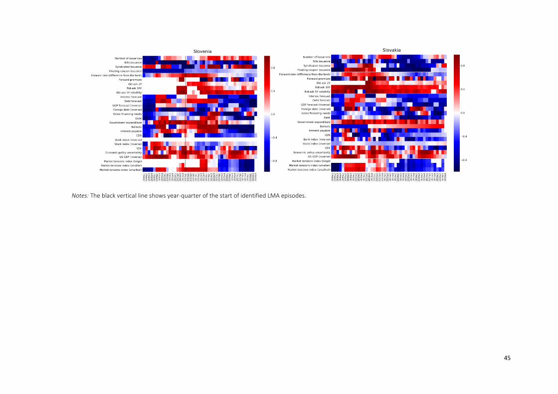
45
Notes: The black vertical line shows year-quarter of the start of identified LMA episodes.
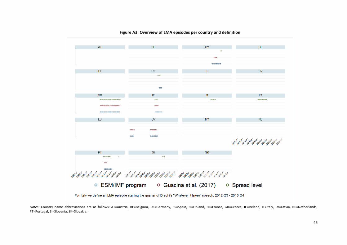
46
Figure A3. Overview of LMA episodes per country and definition
Notes: Country name abbreviations are as follows: AT=Austria, BE=Belgium, DE=Germany, ES=Spain, FI=Finland, FR=France, GR=Greece, IE=Ireland, IT=Italy, LV=Latvia, NL=Netherlands, PT=Portugal, SI=Slovenia, SK=Slovakia.
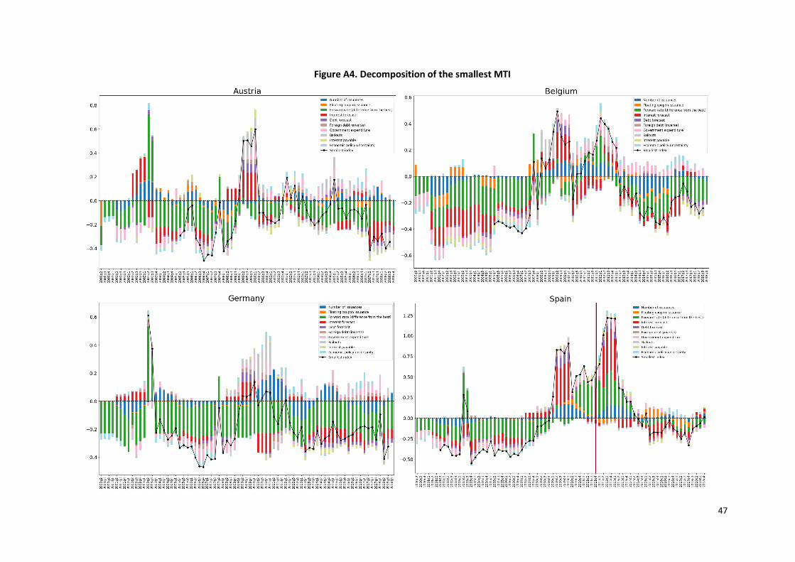
47
Figure A4. Decomposition of the smallest MTI
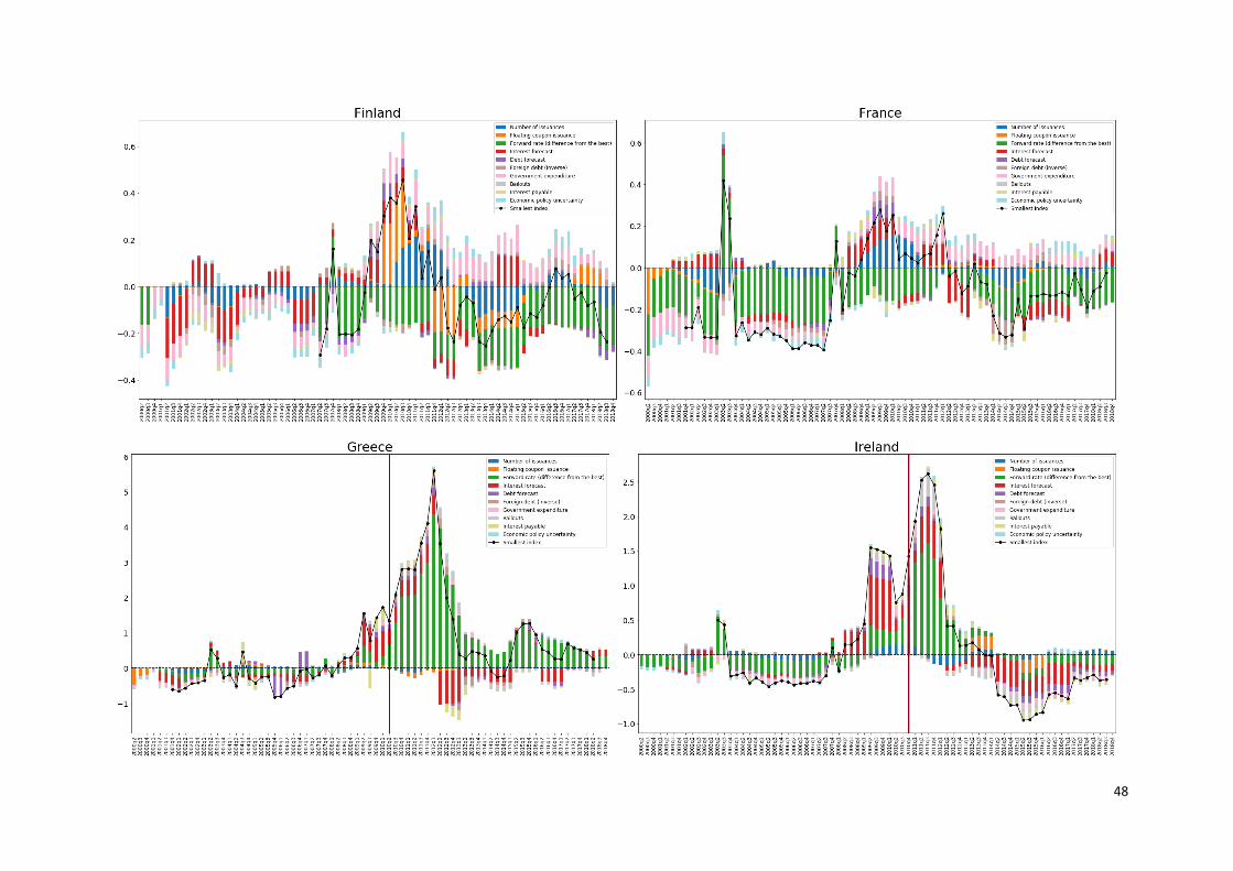
48
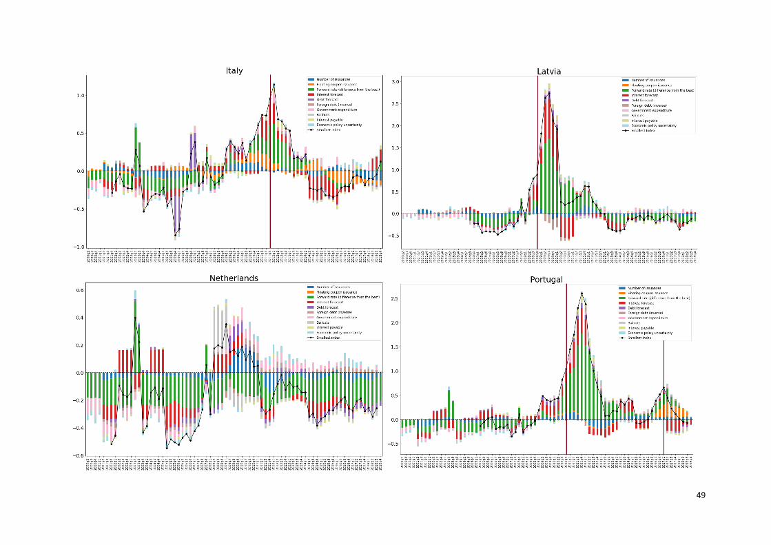
49
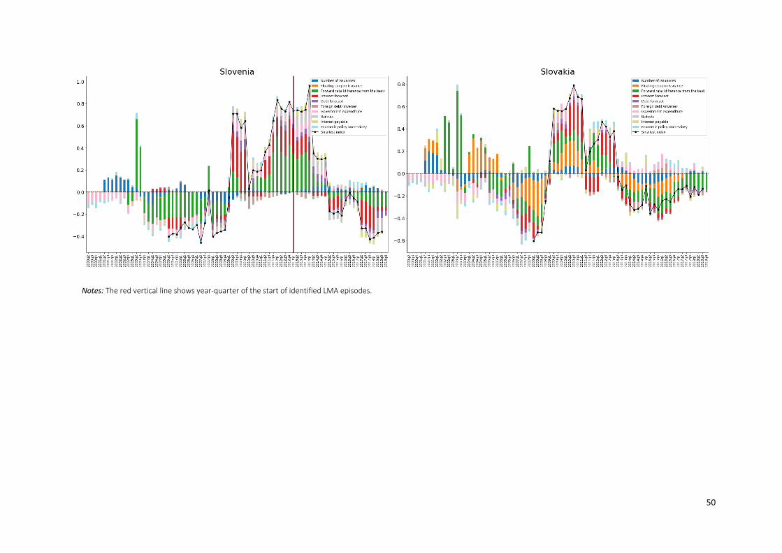
50
Notes: The red vertical line shows year-quarter of the start of identified LMA episodes.

51
Figure A5. LMA identification from alternative spread level definition (two standard deviations above country-specific historical rolling average)
Notes: Country name abbreviations are as follows: AT=Austria, BE=Belgium, DE=Germany, ES=Spain, FI=Finland, FR=France, GR=Greece, IE=Ireland, IT=Italy, LV=Latvia, NL=Netherlands, PT=Portugal, SI=Slovenia, SK=Slovakia.

52
Table A1: Identified top indicators under preference weights of 80%/20% for Type I vs. Type II error
Variable Usefulness Threshold Threshold (percentile) AUC Type I Type II
Primary market
No. of issuances 0.116 -0.064 0.555 0.819 0.000 0.418
Syndicated issuance 0.022 -0.506 0.432 0.674 0.083 0.558
Secondary market
Slope of yield curve 0.169 0.803 0.789 0.949 0.000 0.158
Forward rate (difference from the best) 0.139 -0.242 0.640 0.916 0.000 0.305
Forward premium 0.096 0.026 0.462 0.848 0.000 0.519
Bid-ask 5Y 0.098 -0.276 0.464 0.748 0.000 0.511
Bid-ask 10Y volatility 0.028 -0.153 0.536 0.738 0.105 0.440
Bid-ask 5Y volatility 0.035 -0.151 0.596 0.729 0.111 0.380
Foreign debt (inverse) 0.051 -0.816 0.241 0.670 0.000 0.746
Global demand and supply
CDS 0.025 -0.208 0.589 0.797 0.130 0.354
Government expenditure 0.139 0.172 0.650 0.852 0.000 0.306
GDP forecast (inverse) 0.094 0.394 0.754 0.843 0.083 0.197
Debt 0.061 -0.603 0.277 0.788 0.000 0.695
Interest forecast 0.076 -0.200 0.352 0.797 0.000 0.621
Economic policy uncertainty 0.072 -0.496 0.334 0.727 0.000 0.640
US GDP (inverse) 0.072 -0.488 0.334 0.679 0.000 0.640
VIX 0.073 -0.418 0.334 0.618 0.000 0.634
Ratio of loans to bonds 0.067 -0.540 0.305 0.611 0.000 0.664
Bank index (inverse) 0.019 -0.044 0.515 0.680 0.111 0.460 Notes: AUC stands for the area under receiver’s operating characteristics curve (ROC).
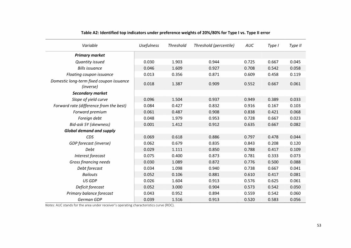
53
Table A2: Identified top indicators under preference weights of 20%/80% for Type I vs. Type II error
Variable Usefulness Threshold Threshold (percentile) AUC Type I Type II
Primary market
Quantity issued 0.030 1.903 0.944 0.725 0.667 0.045
Bills issuance 0.046 1.609 0.927 0.708 0.542 0.058
Floating coupon issuance 0.013 0.356 0.871 0.609 0.458 0.119
Domestic long-term fixed coupon issuance (inverse)
0.018 1.387 0.909 0.552 0.667 0.061
Secondary market
Slope of yield curve 0.096 1.504 0.937 0.949 0.389 0.033
Forward rate (difference from the best) 0.084 0.427 0.832 0.916 0.167 0.103
Forward premium 0.061 0.487 0.908 0.838 0.421 0.068
Foreign debt 0.048 1.979 0.953 0.728 0.667 0.023
Bid-ask 5Y (skewness) 0.001 1.412 0.912 0.635 0.667 0.082
Global demand and supply
CDS 0.069 0.618 0.886 0.797 0.478 0.044
GDP forecast (inverse) 0.062 0.679 0.835 0.843 0.208 0.120
Debt 0.029 1.111 0.850 0.788 0.417 0.109
Interest forecast 0.075 0.400 0.873 0.781 0.333 0.073
Gross financing needs 0.030 1.089 0.872 0.776 0.500 0.088
Debt forecast 0.034 1.098 0.940 0.738 0.667 0.041
Bailouts 0.052 0.106 0.881 0.610 0.417 0.081
US GDP 0.026 1.604 0.913 0.576 0.625 0.061
Deficit forecast 0.052 3.000 0.904 0.573 0.542 0.050
Primary balance forecast 0.043 0.952 0.894 0.559 0.542 0.060
German GDP 0.039 1.516 0.913 0.520 0.583 0.056 Notes: AUC stands for the area under receiver’s operating characteristics curve (ROC).

54
Figure A6. Indicator dynamics vis-à-vis their respective thresholds under unequal preferences: Heatmaps
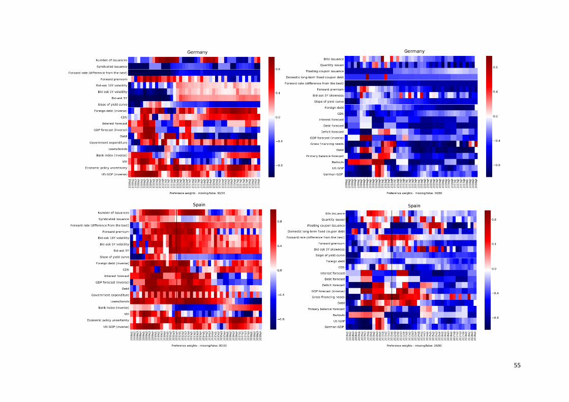
55
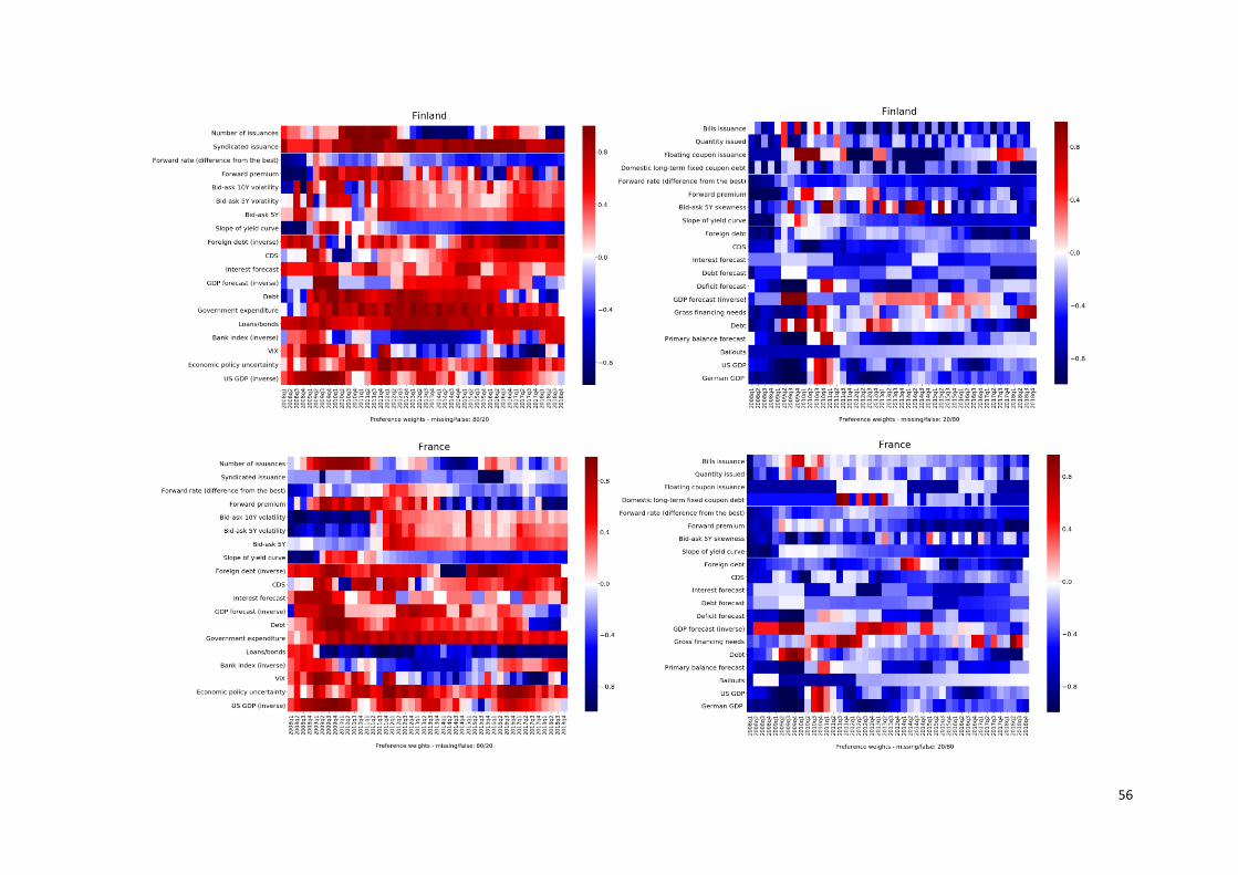
56
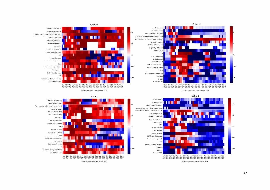
57
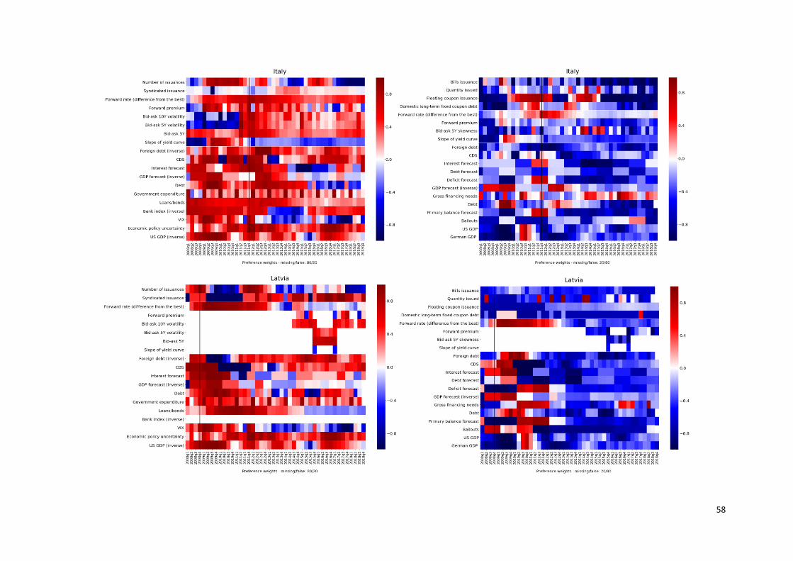
58

59
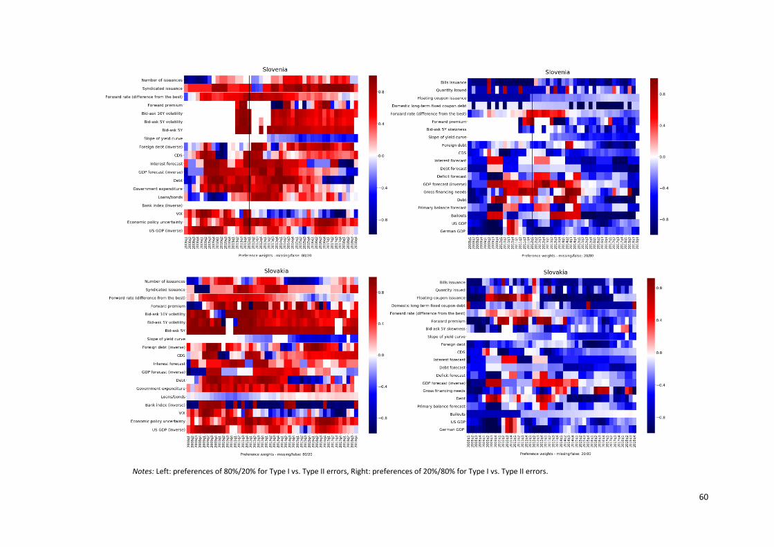
60
Notes: Left: preferences of 80%/20% for Type I vs. Type II errors, Right: preferences of 20%/80% for Type I vs. Type II errors.
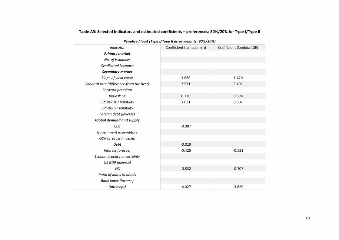
61
Table A3: Selected Indicators and estimated coefficients – preferences: 80%/20% for Type I/Type II
Penalized logit (Type I/Type II error weights: 80%/20%)
Indicator Coefficient (lambda min) Coefficient (lambda 1SE)
Primary market
No. of issuances
Syndicated issuance
Secondary market
Slope of yield curve 1.680 1.420
Forward rate (difference from the best) 3.971 3.491
Forward premium
Bid-ask 5Y 0.720 0.598
Bid-ask 10Y volatility 1.031 0.807
Bid-ask 5Y volatility
Foreign debt (inverse)
Global demand and supply
CDS -0.087
Government expenditure
GDP forecast (inverse)
Debt -0.019
Interest forecast -0.425 -0.181
Economic policy uncertainty
US GDP (inverse)
VIX -0.832 -0.707
Ratio of loans to bonds
Bank index (inverse)
(Intercept) -4.027 -3.829
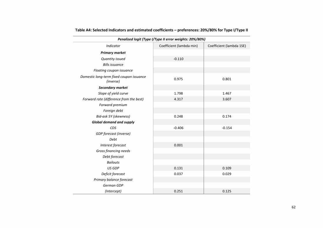
62
Table A4: Selected Indicators and estimated coefficients – preferences: 20%/80% for Type I/Type II
Penalized logit (Type I/Type II error weights: 20%/80%)
Indicator Coefficient (lambda min) Coefficient (lambda 1SE)
Primary market
Quantity issued -0.110
Bills issuance
Floating coupon issuance
Domestic long-term fixed coupon issuance (inverse)
0.975 0.801
Secondary market
Slope of yield curve 1.798 1.467
Forward rate (difference from the best) 4.317 3.607
Forward premium
Foreign debt
Bid-ask 5Y (skewness) 0.248 0.174
Global demand and supply
CDS -0.406 -0.154
GDP forecast (inverse)
Debt
Interest forecast 0.001
Gross financing needs
Debt forecast
Bailouts
US GDP 0.131 0.109
Deficit forecast 0.037 0.029
Primary balance forecast
German GDP
(Intercept) 0.251 0.125
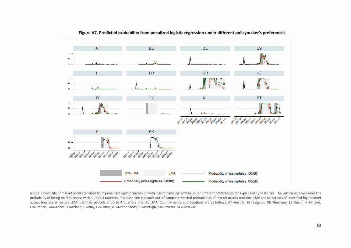
63
Figure A7. Predicted probability from penalized logistic regression under different policymaker’s preferences
Notes: Probability of market access tensions from penalized logistic regression with loss-minimizing lambda under different preferences for Type I and Type II error. The vertical axis measures the probability of losing market access within up to 4 quarters. The dash line indicates out-of-sample predicted probabilities of market access tensions. LMA shows periods of identified high market access tensions while pre-LMA identifies periods of up to 4 quarters prior to LMA. Country name abbreviations are as follows: AT=Austria, BE=Belgium, DE=Germany, ES=Spain, FI=Finland, FR=France, GR=Greece, IE=Ireland, IT=Italy, LV=Latvia, NL=Netherlands, PT=Portugal, SI=Slovenia, SK=Slovakia.
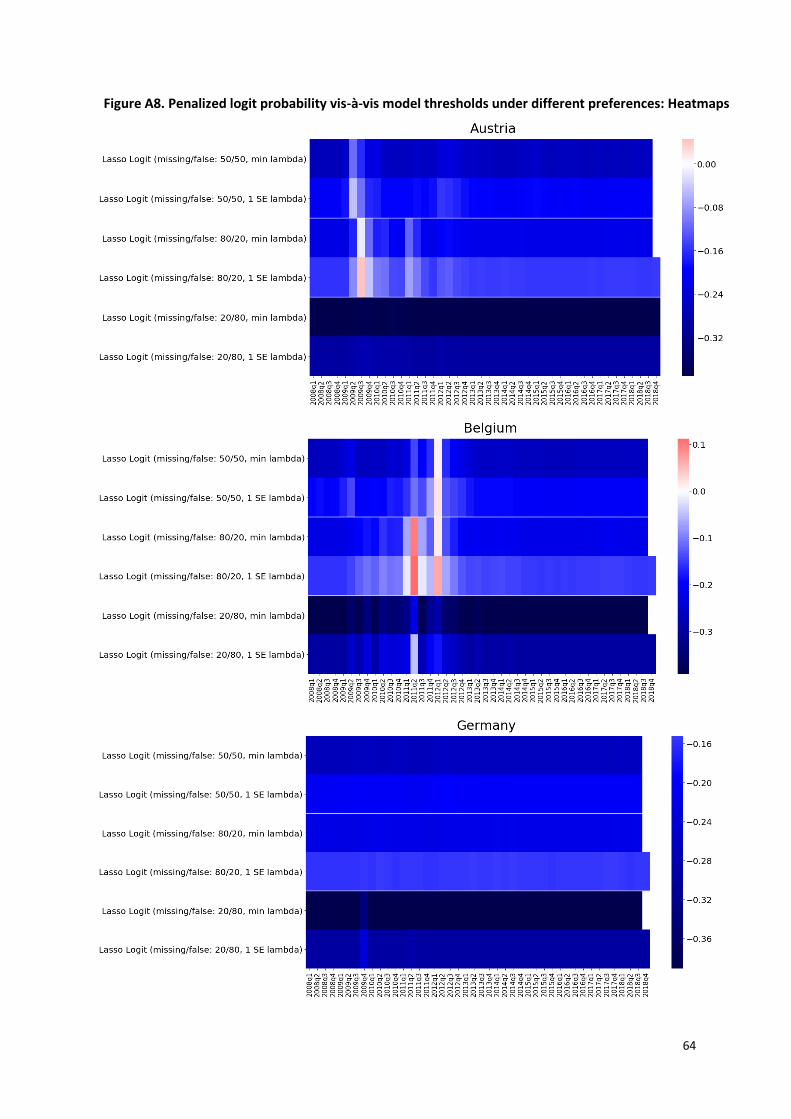
64
Figure A8. Penalized logit probability vis-à-vis model thresholds under different preferences: Heatmaps

65
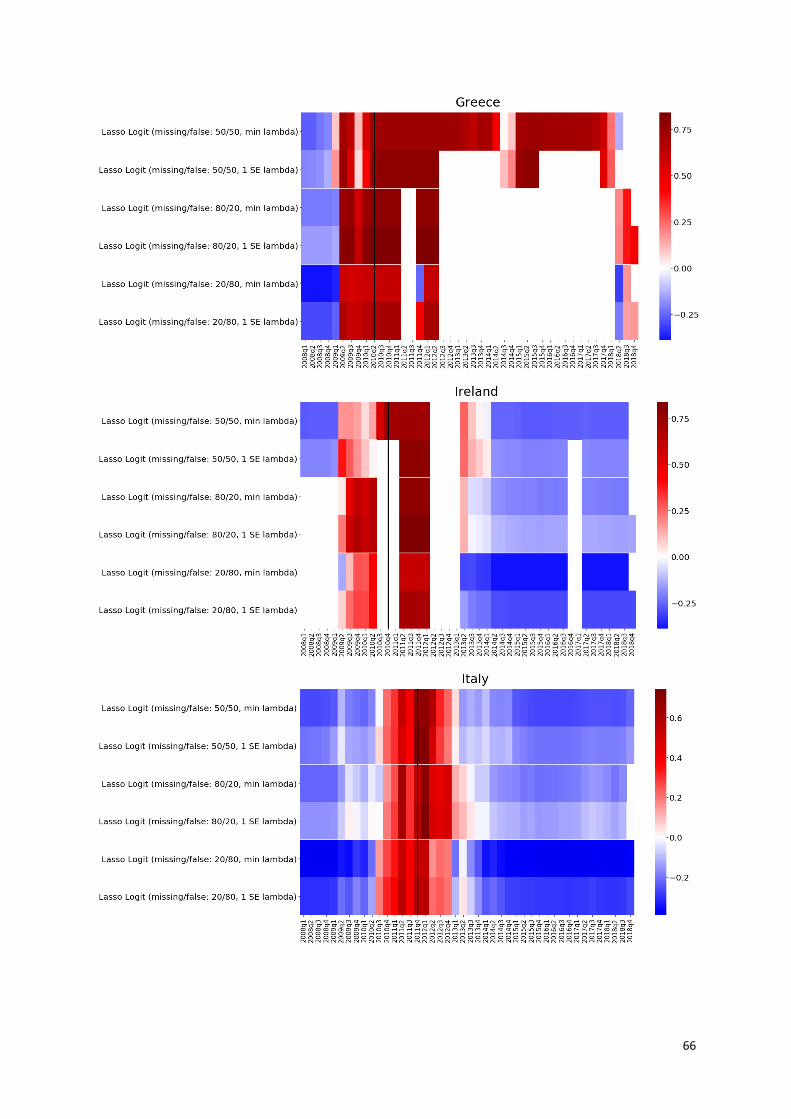
66
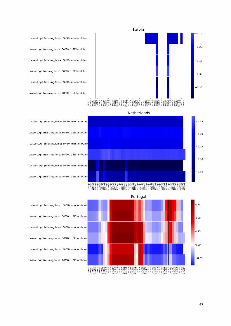
67
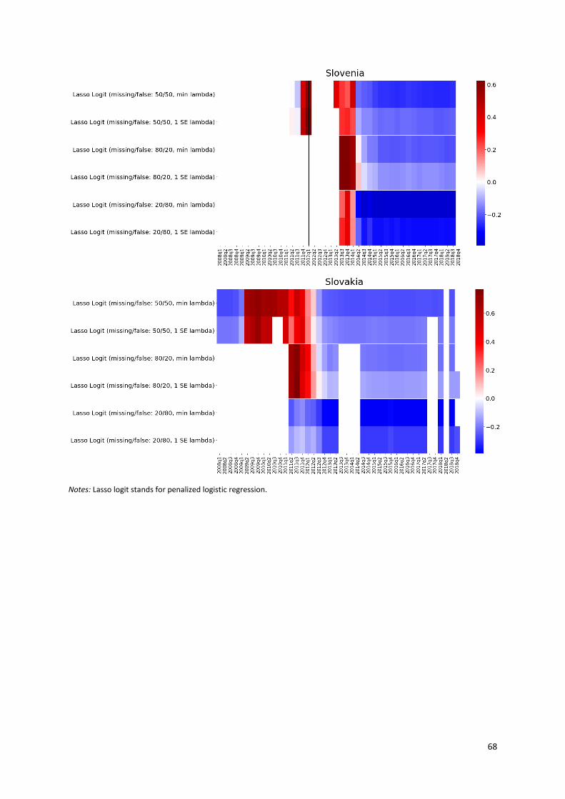
68
Notes: Lasso logit stands for penalized logistic regression.
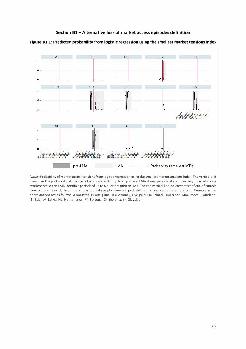
69
Section B1 – Alternative loss of market access episodes definition
Figure B1.1: Predicted probability from logistic regression using the smallest market tensions index
Notes: Probability of market access tensions from logistic regression using the smallest market tensions index. The vertical axis measures the probability of losing market access within up to 4 quarters. LMA shows periods of identified high market access tensions while pre-LMA identifies periods of up to 4 quarters prior to LMA. The red vertical line indicates start of out-of-sample forecast and the dashed line shows out-of-sample forecast probabilities of market access tensions. Country name abbreviations are as follows: AT=Austria, BE=Belgium, DE=Germany, ES=Spain, FI=Finland, FR=France, GR=Greece, IE=Ireland, IT=Italy, LV=Latvia, NL=Netherlands, PT=Portugal, SI=Slovenia, SK=Slovakia.
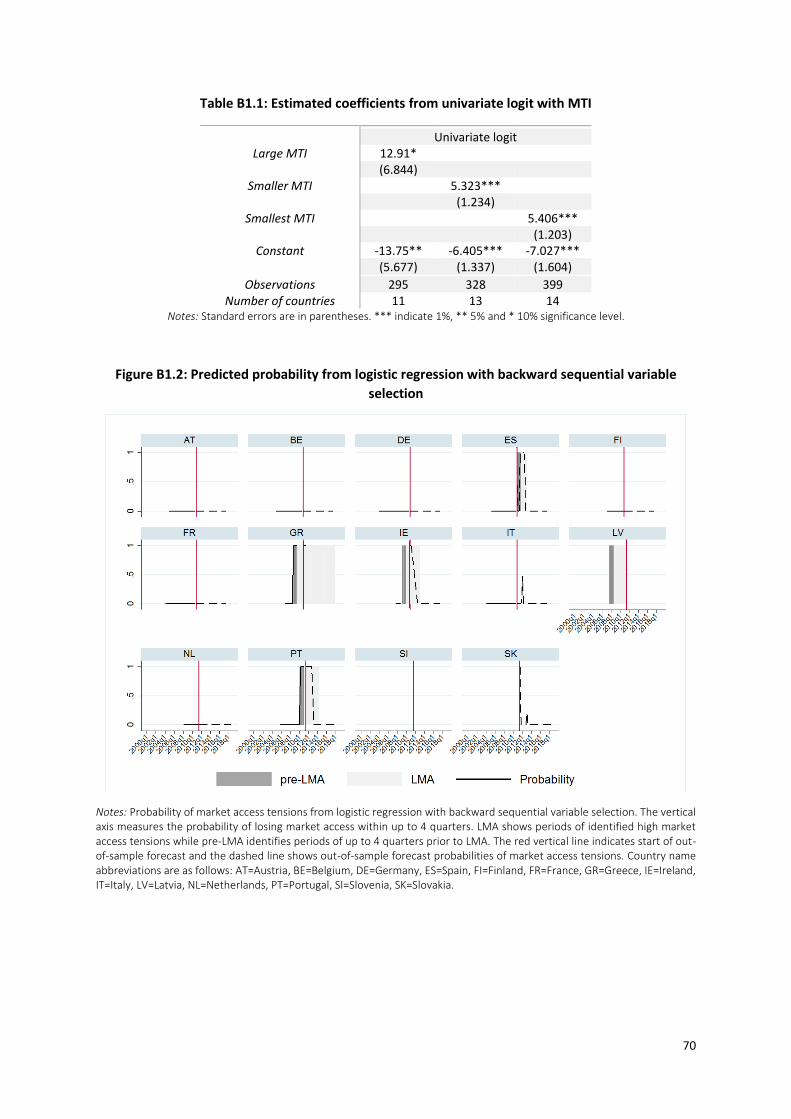
70
Table B1.1: Estimated coefficients from univariate logit with MTI Univariate logit
Large MTI 12.91*
(6.844)
Smaller MTI 5.323*** (1.234)
Smallest MTI 5.406*** (1.203)
Constant -13.75** -6.405*** -7.027*** (5.677) (1.337) (1.604)
Observations 295 328 399 Number of countries 11 13 14
Notes: Standard errors are in parentheses. *** indicate 1%, ** 5% and * 10% significance level.
Figure B1.2: Predicted probability from logistic regression with backward sequential variable
selection
Notes: Probability of market access tensions from logistic regression with backward sequential variable selection. The vertical axis measures the probability of losing market access within up to 4 quarters. LMA shows periods of identified high market access tensions while pre-LMA identifies periods of up to 4 quarters prior to LMA. The red vertical line indicates start of out-of-sample forecast and the dashed line shows out-of-sample forecast probabilities of market access tensions. Country name abbreviations are as follows: AT=Austria, BE=Belgium, DE=Germany, ES=Spain, FI=Finland, FR=France, GR=Greece, IE=Ireland, IT=Italy, LV=Latvia, NL=Netherlands, PT=Portugal, SI=Slovenia, SK=Slovakia.

71
Figure B1.3: Predicted probability from penalized logistic regression
Notes: Probability of market access tensions from penalized logistic regression with loss-minimizing lambda (black line) and with lambda, for which model error is within one standard error of the minimum (brown line). The vertical axis measures the probability of losing market access within up to 4 quarters. LMA shows periods of identified high market access tensions while pre-LMA identifies periods of up to 4 quarters prior to LMA. The red vertical line indicates start of out-of-sample forecast and the dash line shows out-of-sample forecast probabilities of market access tensions. Country name abbreviations are as follows: AT=Austria, BE=Belgium, DE=Germany, ES=Spain, FI=Finland, FR=France, GR=Greece, IE=Ireland, IT=Italy, LV=Latvia, NL=Netherlands, PT=Portugal, SI=Slovenia, SK=Slovakia.
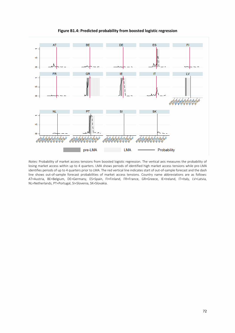
72
Figure B1.4: Predicted probability from boosted logistic regression
Notes: Probability of market access tensions from boosted logistic regression. The vertical axis measures the probability of losing market access within up to 4 quarters. LMA shows periods of identified high market access tensions while pre-LMA identifies periods of up to 4 quarters prior to LMA. The red vertical line indicates start of out-of-sample forecast and the dash line shows out-of-sample forecast probabilities of market access tensions. Country name abbreviations are as follows: AT=Austria, BE=Belgium, DE=Germany, ES=Spain, FI=Finland, FR=France, GR=Greece, IE=Ireland, IT=Italy, LV=Latvia, NL=Netherlands, PT=Portugal, SI=Slovenia, SK=Slovakia.
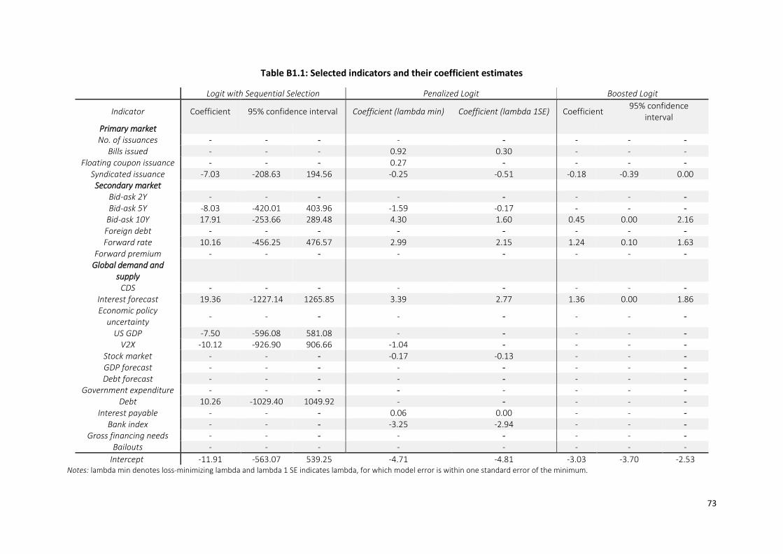
73
Table B1.1: Selected indicators and their coefficient estimates
Logit with Sequential Selection Penalized Logit Boosted Logit
Indicator Coefficient 95% confidence interval Coefficient (lambda min) Coefficient (lambda 1SE) Coefficient 95% confidence
interval Primary market No. of issuances - - - - - - - -
Bills issued - - - 0.92 0.30 - - - Floating coupon issuance - - - 0.27 - - - -
Syndicated issuance -7.03 -208.63 194.56 -0.25 -0.51 -0.18 -0.39 0.00 Secondary market
Bid-ask 2Y - - - - - - - -
Bid-ask 5Y -8.03 -420.01 403.96 -1.59 -0.17 - - -
Bid-ask 10Y 17.91 -253.66 289.48 4.30 1.60 0.45 0.00 2.16 Foreign debt - - - - - - - -
Forward rate 10.16 -456.25 476.57 2.99 2.15 1.24 0.10 1.63 Forward premium - - - - - - - -
Global demand and supply
CDS - - - - - - - -
Interest forecast 19.36 -1227.14 1265.85 3.39 2.77 1.36 0.00 1.86 Economic policy
uncertainty - - - - - - - -
US GDP -7.50 -596.08 581.08 - - - - -
V2X -10.12 -926.90 906.66 -1.04 - - - -
Stock market - - - -0.17 -0.13 - - -
GDP forecast - - - - - - - -
Debt forecast - - - - - - - -
Government expenditure - - - - - - - -
Debt 10.26 -1029.40 1049.92 - - - - -
Interest payable - - - 0.06 0.00 - - -
Bank index - - - -3.25 -2.94 - - -
Gross financing needs - - - - - - - -
Bailouts - - - - - - - -
Intercept -11.91 -563.07 539.25 -4.71 -4.81 -3.03 -3.70 -2.53 Notes: lambda min denotes loss-minimizing lambda and lambda 1 SE indicates lambda, for which model error is within one standard error of the minimum.
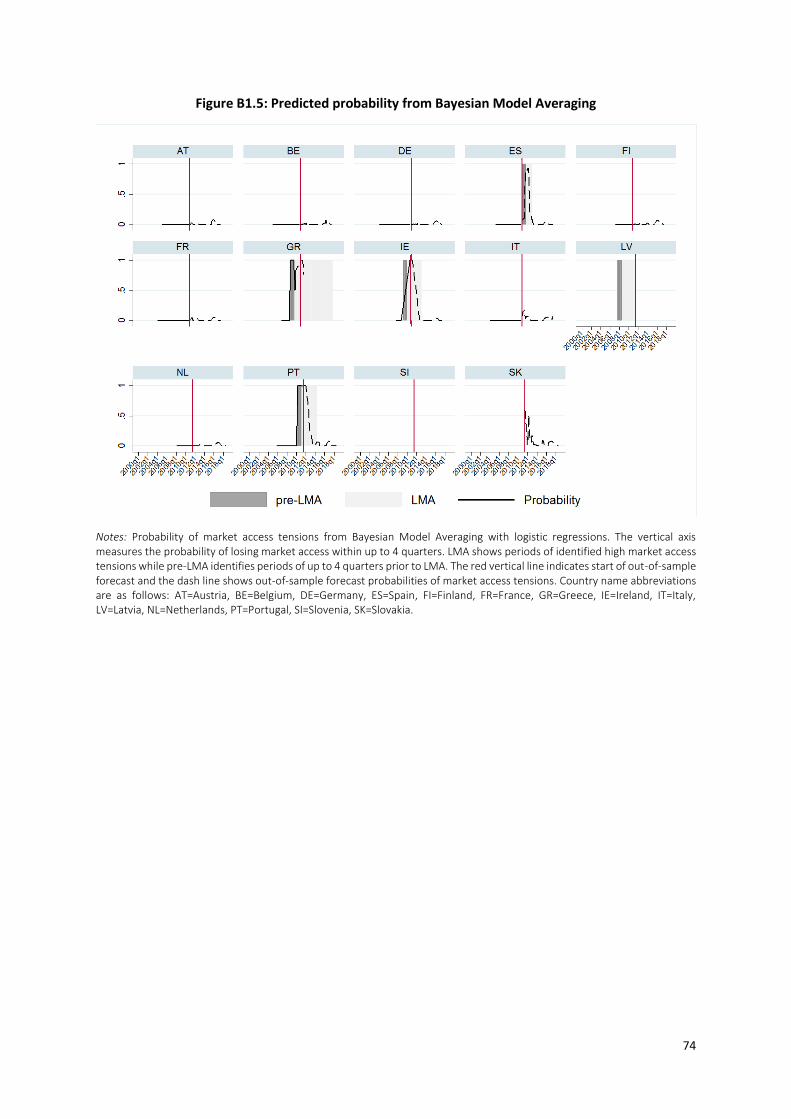
74
Figure B1.5: Predicted probability from Bayesian Model Averaging
Notes: Probability of market access tensions from Bayesian Model Averaging with logistic regressions. The vertical axis measures the probability of losing market access within up to 4 quarters. LMA shows periods of identified high market access tensions while pre-LMA identifies periods of up to 4 quarters prior to LMA. The red vertical line indicates start of out-of-sample forecast and the dash line shows out-of-sample forecast probabilities of market access tensions. Country name abbreviations are as follows: AT=Austria, BE=Belgium, DE=Germany, ES=Spain, FI=Finland, FR=France, GR=Greece, IE=Ireland, IT=Italy, LV=Latvia, NL=Netherlands, PT=Portugal, SI=Slovenia, SK=Slovakia.

75
Figure B1.6: Top 20 models from Bayesian Model Averaging
Notes: Top 20 models from Bayesian Model Averaging ranked (top x-axis) by their posterior model probability from the best (left) to worst (right). Rows correspond to top indicators while columns represent individual models. In each model, missing variables are in black, while included variables are coloured. The colour corresponds to the log of the posterior probability of that model. Posterior probabilities are scaled so that the worst model in the top 20 models is assigned 0. Models with the same colours have similar log Bayes factors, i.e. the difference in their Bayes factors is not worth a mention.
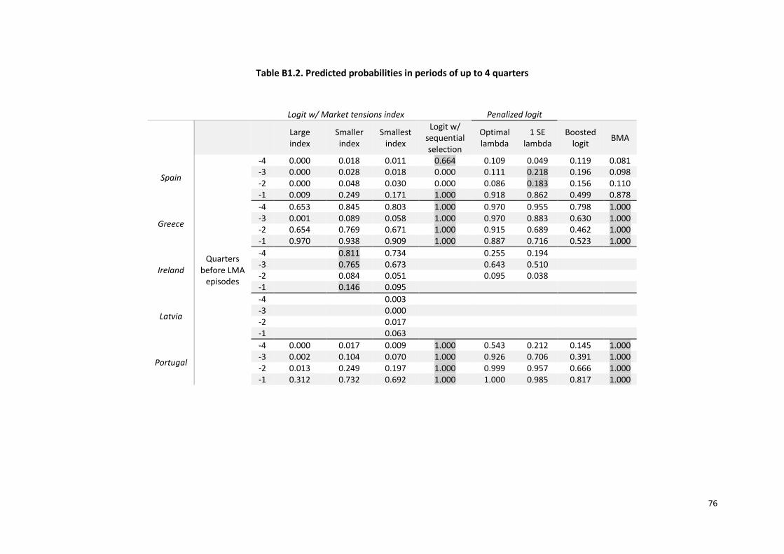
76
Table B1.2. Predicted probabilities in periods of up to 4 quarters
Logit w/ Market tensions index Penalized logit
Large index
Smaller index
Smallest index
Logit w/ sequential selection
Optimal lambda
1 SE lambda
Boosted logit
BMA
Spain
Quarters before LMA
episodes
-4 0.000 0.018 0.011 0.664 0.109 0.049 0.119 0.081 -3 0.000 0.028 0.018 0.000 0.111 0.218 0.196 0.098 -2 0.000 0.048 0.030 0.000 0.086 0.183 0.156 0.110 -1 0.009 0.249 0.171 1.000 0.918 0.862 0.499 0.878
Greece
-4 0.653 0.845 0.803 1.000 0.970 0.955 0.798 1.000 -3 0.001 0.089 0.058 1.000 0.970 0.883 0.630 1.000 -2 0.654 0.769 0.671 1.000 0.915 0.689 0.462 1.000 -1 0.970 0.938 0.909 1.000 0.887 0.716 0.523 1.000
Ireland
-4 0.811 0.734 0.255 0.194
-3 0.765 0.673 0.643 0.510
-2 0.084 0.051 0.095 0.038
-1 0.146 0.095
Latvia
-4 0.003
-3 0.000
-2 0.017
-1 0.063
Portugal
-4 0.000 0.017 0.009 1.000 0.543 0.212 0.145 1.000 -3 0.002 0.104 0.070 1.000 0.926 0.706 0.391 1.000 -2 0.013 0.249 0.197 1.000 0.999 0.957 0.666 1.000 -1 0.312 0.732 0.692 1.000 1.000 0.985 0.817 1.000
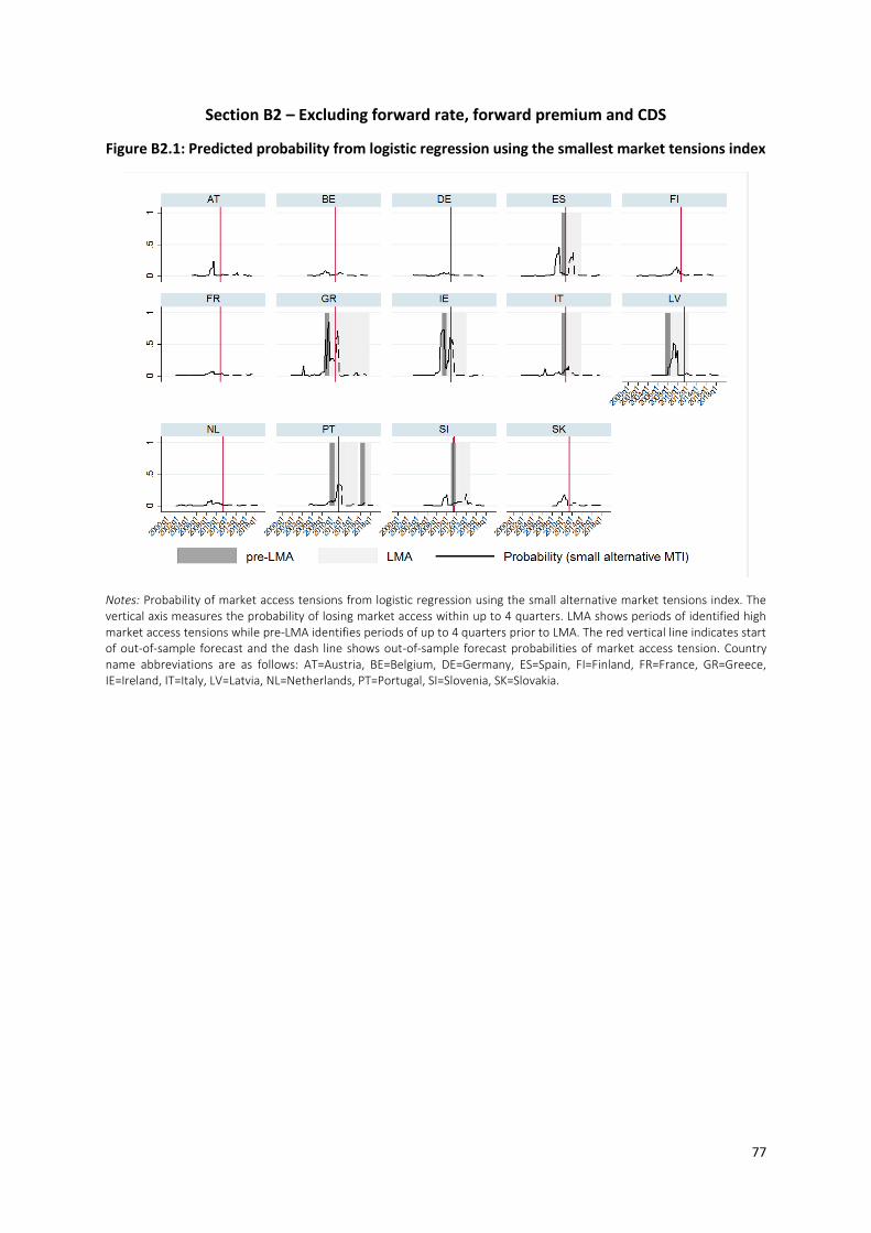
77
Section B2 – Excluding forward rate, forward premium and CDS
Figure B2.1: Predicted probability from logistic regression using the smallest market tensions index
Notes: Probability of market access tensions from logistic regression using the small alternative market tensions index. The vertical axis measures the probability of losing market access within up to 4 quarters. LMA shows periods of identified high market access tensions while pre-LMA identifies periods of up to 4 quarters prior to LMA. The red vertical line indicates start of out-of-sample forecast and the dash line shows out-of-sample forecast probabilities of market access tension. Country name abbreviations are as follows: AT=Austria, BE=Belgium, DE=Germany, ES=Spain, FI=Finland, FR=France, GR=Greece, IE=Ireland, IT=Italy, LV=Latvia, NL=Netherlands, PT=Portugal, SI=Slovenia, SK=Slovakia.
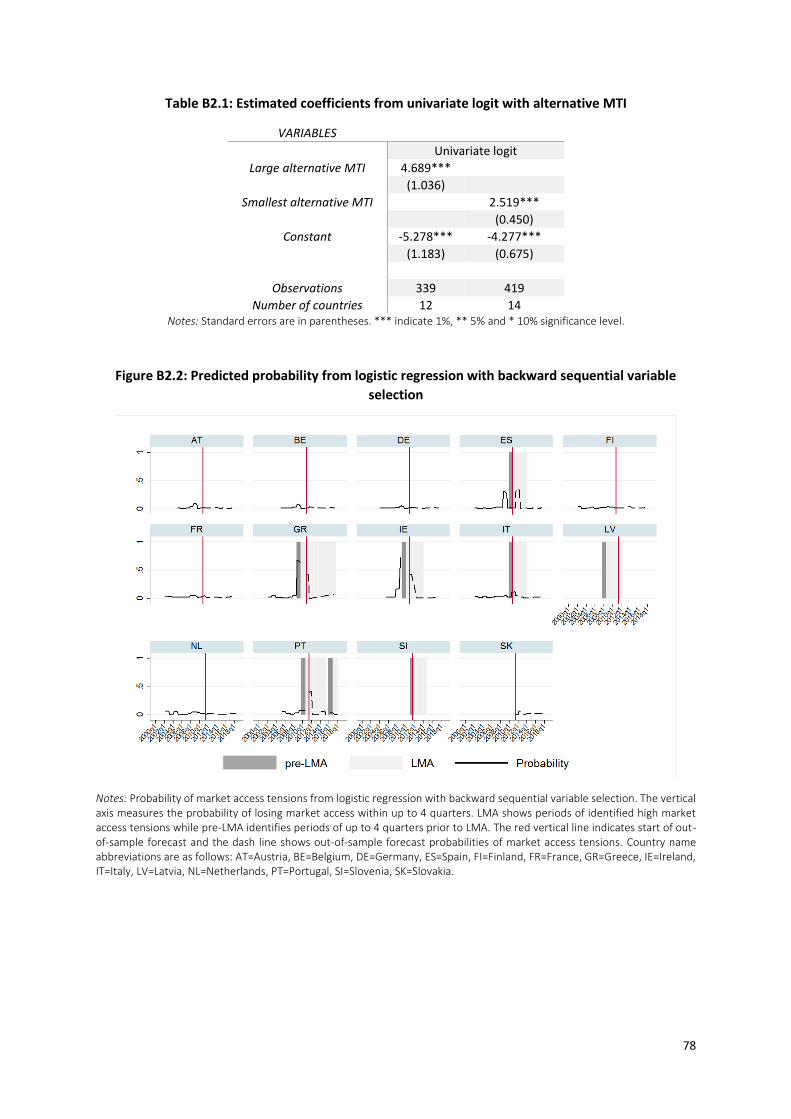
78
Table B2.1: Estimated coefficients from univariate logit with alternative MTI
VARIABLES
Univariate logit
Large alternative MTI 4.689***
(1.036)
Smallest alternative MTI 2.519*** (0.450)
Constant -5.278*** -4.277*** (1.183) (0.675)
Observations 339 419
Number of countries 12 14 Notes: Standard errors are in parentheses. *** indicate 1%, ** 5% and * 10% significance level.
Figure B2.2: Predicted probability from logistic regression with backward sequential variable
selection
Notes: Probability of market access tensions from logistic regression with backward sequential variable selection. The vertical axis measures the probability of losing market access within up to 4 quarters. LMA shows periods of identified high market access tensions while pre-LMA identifies periods of up to 4 quarters prior to LMA. The red vertical line indicates start of out-of-sample forecast and the dash line shows out-of-sample forecast probabilities of market access tensions. Country name abbreviations are as follows: AT=Austria, BE=Belgium, DE=Germany, ES=Spain, FI=Finland, FR=France, GR=Greece, IE=Ireland, IT=Italy, LV=Latvia, NL=Netherlands, PT=Portugal, SI=Slovenia, SK=Slovakia.
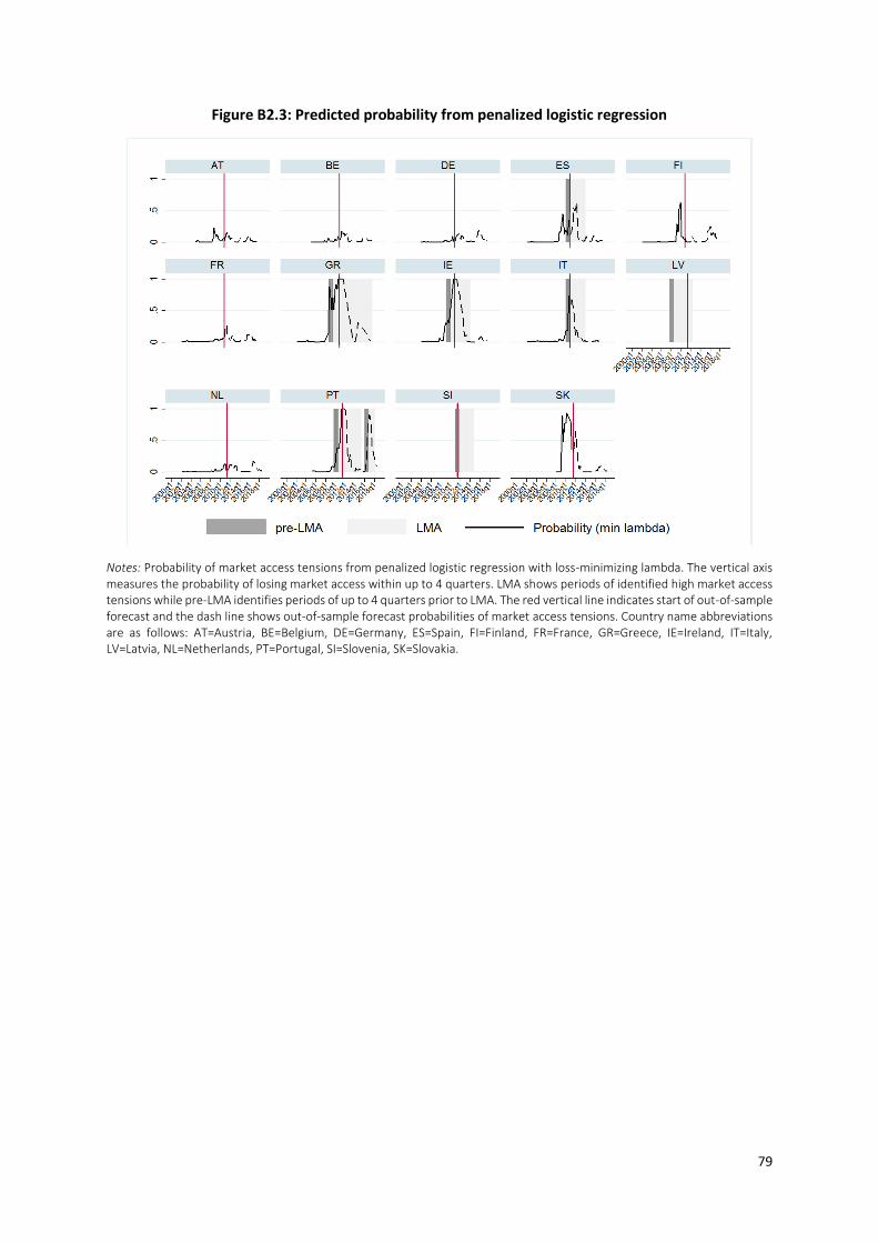
79
Figure B2.3: Predicted probability from penalized logistic regression
Notes: Probability of market access tensions from penalized logistic regression with loss-minimizing lambda. The vertical axis measures the probability of losing market access within up to 4 quarters. LMA shows periods of identified high market access tensions while pre-LMA identifies periods of up to 4 quarters prior to LMA. The red vertical line indicates start of out-of-sample forecast and the dash line shows out-of-sample forecast probabilities of market access tensions. Country name abbreviations are as follows: AT=Austria, BE=Belgium, DE=Germany, ES=Spain, FI=Finland, FR=France, GR=Greece, IE=Ireland, IT=Italy, LV=Latvia, NL=Netherlands, PT=Portugal, SI=Slovenia, SK=Slovakia.
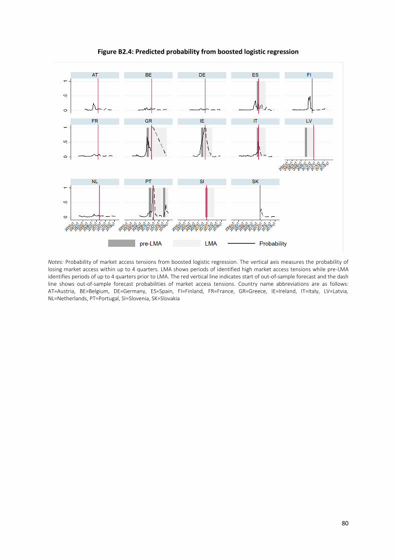
80
Figure B2.4: Predicted probability from boosted logistic regression
Notes: Probability of market access tensions from boosted logistic regression. The vertical axis measures the probability of losing market access within up to 4 quarters. LMA shows periods of identified high market access tensions while pre-LMA identifies periods of up to 4 quarters prior to LMA. The red vertical line indicates start of out-of-sample forecast and the dash line shows out-of-sample forecast probabilities of market access tensions. Country name abbreviations are as follows: AT=Austria, BE=Belgium, DE=Germany, ES=Spain, FI=Finland, FR=France, GR=Greece, IE=Ireland, IT=Italy, LV=Latvia, NL=Netherlands, PT=Portugal, SI=Slovenia, SK=Slovakia
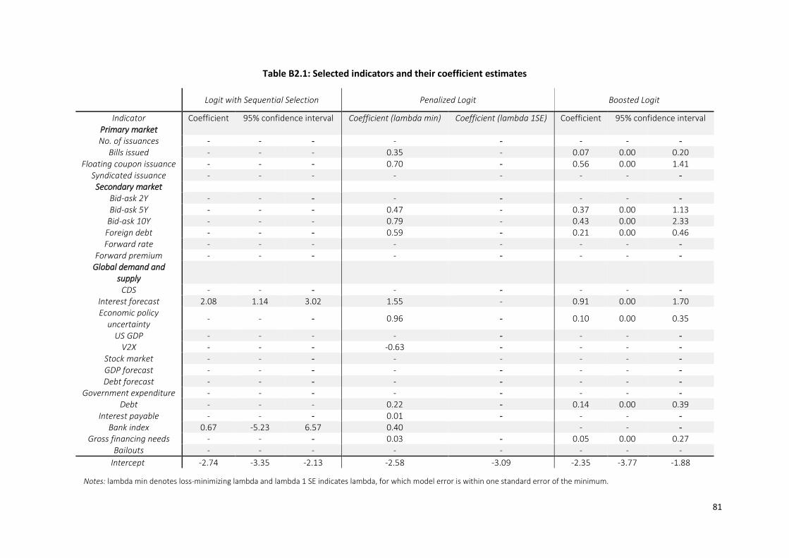
81
Table B2.1: Selected indicators and their coefficient estimates
Logit with Sequential Selection Penalized Logit Boosted Logit
Indicator Coefficient 95% confidence interval Coefficient (lambda min) Coefficient (lambda 1SE) Coefficient 95% confidence interval Primary market No. of issuances - - - - - - - -
Bills issued - - - 0.35 - 0.07 0.00 0.20 Floating coupon issuance - - - 0.70 - 0.56 0.00 1.41
Syndicated issuance - - - - - - - -
Secondary market
Bid-ask 2Y - - - - - - - -
Bid-ask 5Y - - - 0.47 - 0.37 0.00 1.13 Bid-ask 10Y - - - 0.79 - 0.43 0.00 2.33
Foreign debt - - - 0.59 - 0.21 0.00 0.46 Forward rate - - - - - - - -
Forward premium - - - - - - - -
Global demand and supply
CDS - - - - - - - -
Interest forecast 2.08 1.14 3.02 1.55 - 0.91 0.00 1.70 Economic policy
uncertainty - - - 0.96 - 0.10 0.00 0.35
US GDP - - - - - - - -
V2X - - - -0.63 - - - -
Stock market - - - - - - - -
GDP forecast - - - - - - - -
Debt forecast - - - - - - - -
Government expenditure - - - - - - - -
Debt - - - 0.22 - 0.14 0.00 0.39 Interest payable - - - 0.01 - - - -
Bank index 0.67 -5.23 6.57 0.40 - - -
Gross financing needs - - - 0.03 - 0.05 0.00 0.27 Bailouts - - - - - - - -
Intercept -2.74 -3.35 -2.13 -2.58 -3.09 -2.35 -3.77 -1.88
Notes: lambda min denotes loss-minimizing lambda and lambda 1 SE indicates lambda, for which model error is within one standard error of the minimum.

82
Figure B2.5: Predicted probability from Bayesian Model Averaging
Notes: Probability of market access tensions from Bayesian Model Averaging with logistic regressions. The vertical axis measures the probability of losing market access within up to 4 quarters. LMA shows periods of identified high market access tensions while pre-LMA identifies periods of up to 4 quarters prior to LMA. The red vertical line indicates start of out-of-sample forecast and the dash line shows out-of-sample forecast probabilities of market access tensions. Country name abbreviations are as follows: AT=Austria, BE=Belgium, DE=Germany, ES=Spain, FI=Finland, FR=France, GR=Greece, IE=Ireland, IT=Italy, LV=Latvia, NL=Netherlands, PT=Portugal, SI=Slovenia, SK=Slovakia.
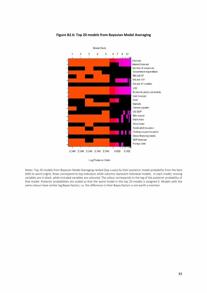
83
Figure B2.6: Top 20 models from Bayesian Model Averaging
Notes: Top 20 models from Bayesian Model Averaging ranked (top x-axis) by their posterior model probability from the best (left) to worst (right). Rows correspond to top indicators while columns represent individual models. In each model, missing variables are in black, while included variables are coloured. The colour corresponds to the log of the posterior probability of that model. Posterior probabilities are scaled so that the worst model in the top 20 models is assigned 0. Models with the same colours have similar log Bayes factors, i.e. the difference in their Bayes factors is not worth a mention.
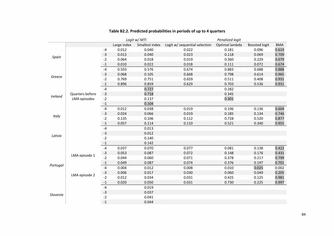
84
Table B2.2. Predicted probabilities in periods of up to 4 quarters
Logit w/ MTI Penalized logit
Large index Smallest index Logit w/ sequential selection Optimal lambda Boosted logit BMA
Spain
Quarters before LMA episodes
-4 0.012 0.040 0.022 0.181 0.096 0.619 -3 0.013 0.040 0.023 0.118 0.069 0.709 -2 0.064 0.018 0.019 0.360 0.229 0.679 -1 0.010 0.022 0.018 0.111 0.072 0.674
Greece
-4 0.503 0.576 0.674 0.883 0.688 0.888 -3 0.068 0.105 0.668 0.798 0.614 0.965 -2 0.769 0.751 0.659 0.511 0.408 0.931 -1 0.896 0.859 0.629 0.703 0.536 0.931
Ireland
-4 0.727 0.282
-3 0.718 0.345
-2 0.137 0.301
-1 0.104
Italy
-4 0.012 0.038 0.019 0.196 0.136 0.604 -3 0.024 0.066 0.019 0.185 0.134 0.746 -2 0.135 0.106 0.112 0.728 0.520 0.877 -1 0.057 0.114 0.110 0.521 0.340 0.955
Latvia
-4 0.013
-3 0.012
-2 0.140
-1 0.142
Portugal
LMA episode 1
-4 0.037 0.070 0.077 0.081 0.138 0.422 -3 0.053 0.087 0.072 0.148 0.176 0.431 -2 0.044 0.060 0.071 0.378 0.217 0.799 -1 0.049 0.087 0.074 0.376 0.197 0.701
LMA episode 2
-4 0.004 0.012 0.008 0.010 0.025 0.002 -3 0.006 0.017 0.030 0.060 0.049 0.205 -2 0.012 0.034 0.031 0.425 0.125 0.981 -1 0.020 0.050 0.031 0.730 0.225 0.997
Slovenia
-4 0.019
-3 0.037
-2 0.041
-1 0.044

6a Circuit de la Foire InternationaleL-1347 Luxembourg
Tel: +352 260 292 0
www.esm.europa.eu
©European Stability Mechanism 1/2020