Quantifying landscape linkages among giant panda subpopulations in regional scale conservation

© 2012 ISZS, Blackwell Publishing and IOZ/CAS 165

123456789

101112131415161718192021222324252627282930313233343536373839404142434445464748495051

123456789101112131415161718192021222324252627282930313233343536373839404142434445464748495051

Quantifying landscape linkages among giant panda subpopulations in regional scale conservation

Dunwu QI,1,2 Yibo HU,2 Xiaodong GU,3 Xuyi YANG,3 Guang YANG1 and Fuwen WEI2

1Jiangsu Key Laboratory for Biodiversity and Biotechnology, College of Life Sciences, Nanjing Normal University, Nanjing, China, 2Key Laboratory for Animal Ecology and Conservation Biology, Institute of Zoology, Chinese Academy of Sciences, Beijing, China and 3Wildlife Conservation Division, Sichuan Forestry Department, Chengdu, China

AbstractUnderstanding habitat requirements and identifying landscape linkages are essential for the survival of isolat-ed populations of endangered species. Currently, some of the giant panda populations are isolated, which threat-ens their long-term survival, particularly in the Xiaoxiangling mountains. In the present study, we quantified niche requirements and then identified potential linkages of giant panda subpopulations in the most isolated re-gion, using ecological niche factor analysis and a least-cost path model. Giant pandas preferred habitat with co-nifer forest and gentle slopes (>20 to ≤30°). Based on spatial distribution of suitable habitat, linkages were iden-tified for the Yele subpopulation to 4 other subpopulations (Liziping, Matou, Xinmin and Wanba). Their lengths ranged from 15 to 54 km. The accumulated cost ranged from 693 to 3166 and conifer forest covered over 31%. However, a variety of features (e.g. major roads, human settlements and large unforested areas) might act as barriers along the linkages for giant panda dispersal. Our analysis quantified giant panda subpopulation connec-tivity to ensure long-term survival.

Key words: Ailuropoda melanoleuca, ecological niche factor analysis, giant panda, landscape connectivity, least-cost path analysis, species conservation

Integrative Zoology 2012; 7: 165–174 doi: 10.1111/j.1749-4877.2012.00281.x

ORIGINAL ARTICLE

Correspondence: Fuwen Wei, Institute of Zoology, Chinese Academy of Sciences, 1-5 Beichenxi Road, Chaoyang, Beijing 100101, China. Email: [email protected]

INTRODUCTION The destruction and fragmentation of continuous hab-

itats into small and isolated patches is taking place all over the world, threatening the survival of many endan-gered species (Wilcox & Murphy 1985; Caughley 1994; Harrison & Bruna 1999; Fahrig 2003; Husté & Boulin-

ier 2007). Maintaining and restoring landscape linkag-es to connect suitable habitat patches is recognized as an important goal for wildlife conservation (Rayfield et al. 2010). Such linkages are increasingly becoming the main parts of regional conservation planning (Lar-kin et al. 2004). However, the identification of conser-vation linkages typically neglects processes of habitat selection for target organisms (Chetkiewicz et al. 2006). Fortunately, resource selection models and least-cost path (LCP) analysis provide a quantitative, functionally-based and repeatable way to identify potential linkages for animal conservation (Chetkiewicz & Boyce 2009).

The giant panda [Ailuropoda melanoleuca (David, 1869)] is an endangered species that occurs across the

© 2012 ISZS, Blackwell Publishing and IOZ/CAS166

123456789

101112131415161718192021222324252627282930313233343536373839404142434445464748495051

D. Qi et al.

eastern edge of the Tibetan Plateau (Hu 2001). Recent studies indicate that its population and habitat are in-creasing (SFA 2006; Zhan et al. 2006) and that this spe-cies still possesses a relatively high genetic diversity (Zhang et al. 2007). However, habitat fragmentation is increasingly impacting the long-term survival of small and isolated populations of giant pandas (Swaisgood et al. 2011; Zhu et al. 2010, 2011). A total of 1596 wild giant pandas are restricted to 24 discontinuous popu-lations isolated by mountain ranges, rivers, roads, for-est clearings and human settlements across 6 separate mountain ranges where bamboo dominates the forest understorey (SFA 2006; Wang et al. 2010). Some pop-ulations have fewer than 20 individuals. These popula-tions are considered too small to persist, especially in the Xiaoxiangling Mountains (Zhu et al. 2010, 2011).

Natural barriers (e.g. Dadu River) and anthropogenic effects (e.g. human settlements, deforestation and roads) have left the Xiaoxiangling giant panda population iso-lated from its neighboring populations, such as the Dax-iangling and Liangshan populations. As a result of hu-man-induced deforestation and habitat fragmentation, the population has experienced a demographic collapse (Zhu et al. 2010). Currently, the Xiaoxiangling popula-tion has only 32 individuals, which are divided into iso-lated insular subpopulations (SFA 2006). To support the survival and persistence of this population, it is impor-tant to determine the niche requirements of individuals and to identify potential landscape linkages among iso-lated subpopulations.

Currently, spatial explicit model (i.e. ecological niche factor analysis, ENFA) and LCP analysis are widely used to identify species niche requirements (Hirzel et al. 2002) and optimal landscape linkages (Barrows et al. 2011). Applying these analyses, we intend to address the following questions related to conservation planning for giant pandas in Xiaoxiangling: What are the niche re-quirements of the giant panda and where are the suitable habitats and potential linkages to connect isolated sub-populations?

MATERIALS AND METHODS

Study area

The Xiaoxiangling Mountains (101°39′–102°28′E, 28°7′–29°32′N), situated at the most south-western range of the giant panda distribution, encompasses ap-proximately 7470 km2, and occupies parts of Jiulong, Mianning and Shimian Counties (Fig. 1). The bound-

ary of Xiaoxiangling is defined according to geograph-ic features (e.g. rivers and mountain ridges), administra-tive borders and giant panda habitat distribution.

Species and ecogeographical variables mapping

From June to September 2001, field observers per-formed transect surveys and searched for signs of giant pandas (e.g. feces, foraging sites and dens). Based on knowledge of giant panda habitat distribution, 2 strata transects were used: 2 and 6 km2 in the known and po-tential distribution range, respectively. Field observers established transects along altitudinal gradients, ensur-ing that each transect sampled all representative habitat types. Using the Global Positioning System (GPS), field observers recorded locations at the start and end points of each transect and at points every 200 m along the transect. In the present study, a total of 88 presence lo-cations were used for analysis. Presence locations with-in a distance of 12.5 km from each other were deter-mined to be from the same subpopulation, based on the dispersal distance of giant pandas (Hu et al. 2010). As a result, 5 subpopulations (Liziping, Matou, Xinmin, Yele and Wanba) were found in Xiaoxiangling (Fig. 1).

Based on documented species–habitat associations (Hu 2001; Qi et al. 2009), ecogeographical variables (EGVs) related to terrain, land cover and human distur-bance were prepared (Table 1). A total of 13 topographic variables were derived from the digital elevation mod-el (DEM) from the International Scientific and Techni-cal Data Mirror Site, Computer Network Information Center, Chinese Academy of Sciences (http://datamirror.csdb.cn).

Vegetation was mapped using a Landsat 5 scene ac-quired in April 2002 and May 2006, which was ob-tained from the Global Land Cover Facility (Univer-sity of Maryland, College Park, USA). Xiaoxiangling Range has complex and rugged terrain, and the vege-tation has a vertical distribution pattern. In such areas, different cover types that have similar spectral charac-teristics might occupy different elevation zones, slopes or aspects. Therefore, we used both ERDAS Imagine 8.7 and ARCGIS 9.2 to integrate the data (using stan-dard Geographic Information System [GIS] features) and DEM by contour mapping. Ground truth data were taken at 126 points from 2004 and 2005 field surveys in to verify classified vegetation maps. Misclassified areas were identified and corrected manually using ARCGIS 9.2 software. After correction with ground truth data, the kappa accuracy index was used to evaluate the clas-sification accuracy. Generally, values of the kappa index


123456789101112131415161718192021222324252627282930313233343536373839404142434445464748495051

Identifying habitat linkages

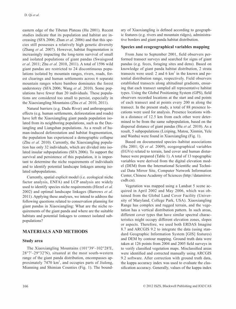
Figure 1 Study area based on giant pan-das distribution (hollow circle) range in the Xiaoxiangling (XXL) moun-tains, Sichuan, China. Seven core hab-itat areas (green) were generated, and the 4 linkages (brown) were identi-fied between the source area (darker green) and the other 4 subpopulations (blue) in XXL: YX (Yele-Xinmin), YL (Yele-Liziping), YM (Yele-Matou) and YW (Yele-Wanba). Two protected ar-eas (Liziping and Yele Nature Reserve) were established in XXL.

higher than 0.75 reflect greater accuracy. In the pres-ent study, the accuracy of the land cover classification was above 0.79. Using the maximum likelihood classi-fication algorithm in supervised classification, 5 class-es were created by ERDAS 8.7 (Leica Geosystems GIS and Mapping 2003): conifer forest (20.4% of the total area), mixed forest (37.4%), evergreen and deciduous broadleaf forest (2.3%), shrub (15.6%) and arable land/others (24.3%). All variables were converted to raster maps in ArcGIS, with a 30 m resolution.

To calculate habitat suitability, 2 classes of quantita-tive raster maps describing EGVs were included: fre-quency and distance variables. Frequency variables, cal-culated using the CiracAn of Biomapper (Hirzel et al. 2007), describe the frequence of occurrence of a habitat characteristic with a 1380 m radius, the average home range (Schaller et al. 1985). Distance variables, cal-culated using DistAn v1.3.1.19 in Biomapper (Hirzel et al. 2007), measure the distance between the focal lo-cation and the closest grid belonging to a given catego-

ry. As a result, a total of 38 variables were prepared (Ta-ble 1). However, when a correlation coefficient between 2 variables was greater than 0.5, only 1 could be re-tained (Engler et al. 2004). To check correlations among 38 variables, we produced a correlation tree in Biomap-per, removed 1 variable from each correlated pair and launched ENFA again. We repeated this step until all the correlation coefficients were less than 0.5. A total of 16 variables were retained in the final model (Table 2).

Habitat suitability modeling

Applying a presence-only approach, ENFA uses the distribution of species records to summarize descrip-tors into a few independent components that are related to the species ecological niche (Hirzel et al. 2002). The first factor explains all species’ marginality, which refers to the degree to which the species’ mean differs from the global mean across the study area. Other factors explain specialization, which measures niche narrowness rela-tive to global variance (Hirzel et al. 2002), and high ab-solute values of specialization indicate a more restricted


123456789

101112131415161718192021222324252627282930313233343536373839404142434445464748495051

D. Qi et al.

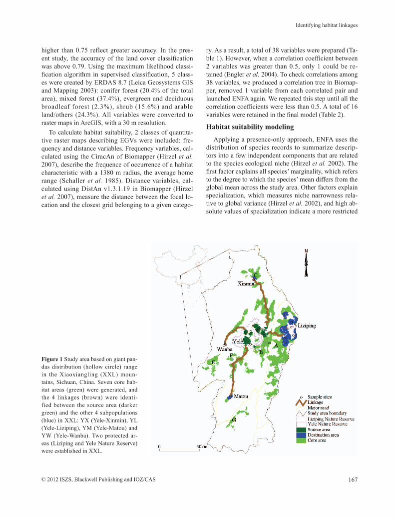
Table 1 Ecogeographical variables (EGVs) included in the ecological niche factor analysis (ENFA). Frequency variables describe the proportion of cells containing a given feature within a 1380 m radius of a location where giant panda presence was found; dis-tance variables measure the distance between the same location and the closest cell containing a given feature

EGV DescriptionAl-fq Frequency of arable land within a 1380 m radius from focal cellAltitude Average height in meters above sea level of focal cellCf-fq Frequency of conifer forest within a 1380 m radius from focal cellDis-major road (km) Average distance from focal cell to roads connecting counties (major roads), blacktopped roads

which had more vehicles than minor roadsDis-minor road (km) Average distance from focal cell to roads connecting towns (minor roads), unpaved roads with

fewer vehiclesDis-Al (km) Average distance from focal cell to arable landsDis-CF (km) Average distance from focal cell to conifer forests Dis-east (km) Average distance from focal cell to east-facing slopes (45–135°)Dis-ED (km) Average distance from focal cell to evergreen and deciduous broadleaf forests Dis-MF (km) Average distance from focal cell to mixed coniferous and deciduous broadleaf forests

Dis-north (km) Average distance from focal cell to north-facing slopes (315–45°)Dis-SH (km) Average distance from focal cell to shrubsDis-slope10 (km) Average distance from focal cell to ≥ 0 to ≤10° slopes Dis-slope20 (km) Average distance from focal cell to >10 to ≤20° slopesDis-slope30 (km) Average distance from focal cell to >20 to ≤30° slopesDis-slope40 (km) Average distance from focal cell to >30 to ≤40° slopesDis-slope50 (km) Average distance from focal cell to >40 to ≤50° slopesDis-slope60 (km) Average distance from focal cell to >50 to ≤60° slopesDis-slope6090 (km) Average distance from focal cell to >60 to ≤90° slopesDis-south (km) Average distance from focal cell to south-facing slopes (135–225°) Dis-town (km) Average distance from focal cell to townsDis-village (km) Average distance from focal cell to villages Dis-west (km) Average distance from focal cell to west-facing slopes (225–315°)East-fq Frequency of east-facing slopes (45–135°) within a 1380 m radius from focal cellED-fq Frequency of evergreen and deciduous broadleaf forests within a 1380 m radius from focal cellMF-fq Frequency of mixed coniferous and deciduous broadleaf forests within a 1380 m radiusNorth-fq Frequency of north-facing slopes (315–45°) within a 1380 m radius from focal cellSH-fq Frequency of shrubs within a 1380 m radius from focal cellSlope10-fq Frequency of ≥ 0 to ≤10° slopes within a 1380 m radius from focal cellSlope20-fq Frequency of >10 to ≤20° slopes within a 1380 m radius from focal cellSlope30-fq Frequency of >20 to ≤30° slopes within a 1380 m radius from focal cellSlope40-fq Frequency of >30 to ≤40° slopes within a 1380 m radius from focal cellSlope50-fq Frequency of >40 to ≤50° slopes within a 1380 m radius from focal cellSlope60-fq Frequency of >50 to ≤60°slopes within a 1380 m radius from focal cellSlope60-90-fq Frequency of >60 to ≤90° slopes within a 1380 m radius from focal cellSlope-mean Mean angle of slopes within a 1380 m radius from focal cellSouth-fq Frequency of south-facing slopes (135–225°) within a 1380 m radiusWest-fq Frequency of west-facing slopes (225–315°) within a 1380 m radius


123456789101112131415161718192021222324252627282930313233343536373839404142434445464748495051


range of the species for a given variable (Engler et al. 2004).

To provide overall information about the niche of a species, global marginality and specialization coef-ficients integrate these descriptor-specific scores (Hir-zel et al. 2007). Global marginality (ranging from 0 to 1) measures how much the average environmental condi-tions selected by the species are different from the av-erage environmental conditions in the study area (the higher the marginality, the more extreme the conditions in the area studied). The global tolerance coefficient, de-fined as the inverse of the specialization (ranging from 0 to 1) and indicates niche breadth of species, with low values indicating a specialist species and high values in-dicating a tolerant species (Hirzel et al. 2004).

Mapping habitat suitability for giant pandas

Habitat suitability maps were calculated by the me-dian algorithm based on several factors obtained by the

ENFA (Hirzel et al. 2002). Based on MacArthur’s bro-ken-stick distribution (Jackson 1993), these factors were derived from a comparison of variables’ eigenvalues, a count of species presence compared to the median of the whole study area conditions (Sattler et al. 2007). Over-all habitat suitability (ranging from 0 to 100), an indica-tion of how the environmental combination of a single cell suits the requirement of a study species, was calcu-lated by combining the score of each factor (Hirzel & Arlettaz 2003). The quality of habitat suitability mod-eling was assessed using the Boyce index (B), of which a value greater than 0.5 indicated a good model (Hirzel et al. 2006). Based on the Boyce index, highly suitable areas were defined as those that giant pandas preferred or facilitated dispersal (habitat suitability >50), unsuit-able areas were defined as those that giant pandas avoid-ed or that impeded dispersal (habitat suitability <20) and the areas between 20 and 50 were defined as moderately suitable.

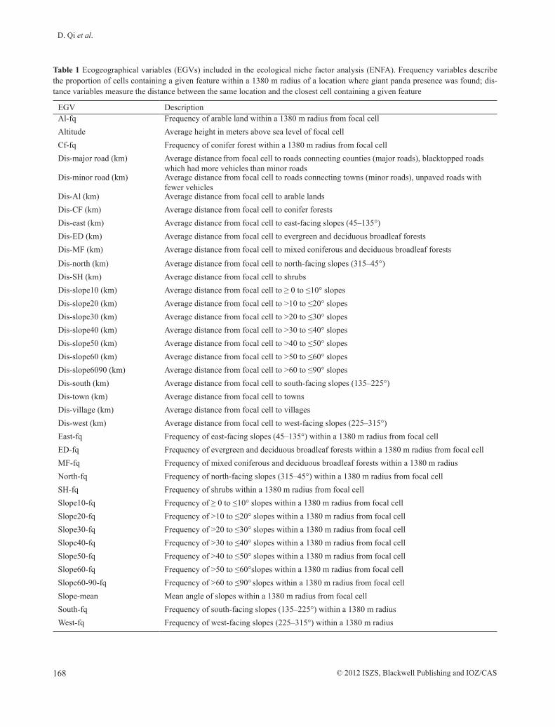
Table 2 Coefficients of each ecogeographical variable (EGV) in the ecological niche factor analysis (ENFA) model of giant pandas in the Xiaoxiangling mountains

Ecogeographical variablesMarginality

(71%)Specialization 1



(4%)Cf-fq 0.75 –0.07 –0.10 –0.13 Dis-Al 0.16 0.04 0.03 0.10 Dis-ED –0.27 –0.64 –0.42 –0.31 Dis-major road 0.01 –0.17 0.16 –0.38 Dis-minor road –0.22 0.00 0.05 0.62 Dis-MF –0.17 0.05 0.69 –0.26 Dis-slope10 –0.06 0.00 0.03 0.03 Dis-slope20 –0.17 –0.01 –0.13 0.02 East-fq 0.03 –0.05 –0.08 –0.01 North-fq –0.04 0.04 –0.05 0.08 Slope10-fq –0.13 0.70 –0.52 –0.35 Slope20-fq 0.16 –0.13 0.03 0.18 Slope30-fq 0.36 0.08 –0.07 –0.09 Slope60-90-fq –0.20 0.17 –0.07 –0.26 South-fq –0.08 –0.02 0.01 –0.09 West-fq 0.01 0.05 –0.03 0.17

Marginality refers to the degree to which the species’ mean differs from the global mean across the study area. The marginality co-efficient attributed to each variable is high when species presence is farther from the mean value of the area. Negative coefficients indicate that the species prefers values that are lower than the mean value of the variable. Specialization measures niche narrowness relative to the global variance. High absolute values of specialization mean a more restricted range of the species for a given vari-able.


123456789

101112131415161718192021222324252627282930313233343536373839404142434445464748495051

D. Qi et al.

Determining core habitat areas for giant pandas

To identify core habitat areas, we followed methods outlined by Titeux et al. (2007) and Chen et al. (2000). Core habitat should include more than 50% species presence (Titeux et al. 2007) and at least 20 km2 (Chen et al. 2000). In the present study, habitat with 50% spe-cies presence corresponds to a habitat suitability val-ue of 50. An area of 20 km2 is a minimum area needed to sustain a small population with at least 5 individuals over the short term (Shen et al. 2008). Therefore, hab-itat with a >50 suitability value and more than 20 km2 was defined as ‘core habitat’. However, if barriers (e.g. major roads, main rivers and arable land) existed with-in the core habitat identified, the area was divided into 2 different core habitats.

Identifying linkage and potential bottlenecks

We used ArcView 3.3 and the LCP analysis to iden-tify potential linkages between giant panda subpopula-tions based on a habitat suitability map. The LCP analy-sis is based on the hypothesis that high habitat suitability means low cost, and vice versa (Kindall & van Manen 2007). The relative cost of the cell for dispersal is com-puted as 100 minus the habitat suitability value of the respective cell. Based on habitat suitability maps, giant pandas are more likely to disperse along the least-resis-tance path between subpopulations. Therefore, the LCP analysis can be used to find the optimal linkage among subpopulations of giant pandas.

Based on the spatial distribution of panda subpop-ulations in the Xiaoxiangling, linkages were devel-oped from the center subpopulation of Yele to 4 oth-er surrounding subpopulations in Xiaoxiangling by LCP (Adriaensen et al. 2003; Ray 2005). The ranges of sub-populations were delimited by buffering presence loca-tions of giant pandas by 2760 m (average home range diameter), and then the closest sites from source area (Yele subpopulation) to destination area (the other 4 subpopulations) were determined as the start and end points of the linkage. Potential linkage bottlenecks that increase habitat resistance and impede giant panda dis-persal were determined based on unsuitable habitat and physical barriers (i.e major roads, human settlements and large unforested areas).

To comprehensively understand the landscape char-acteristics of the linkage, we buffered the linkage iden-tified by 2250 m on each side, a distance that is suffi-cient for giant panda movement through a linkage (Chen et al. 2000). We then extracted EGV factors (e.g. coni-

fer forest and slope) within each linkage’s buffer area by ArcView 3.3 (ESRI, California, USA). Using FRAG-STATS (McGarigal et al. 2002), we analyzed these land-scape characteristics and evaluated their practicability.

RESULTS

Niche requirements analysis

The ENFA computed a global marginality coeffi-cient of 0.947 and a global tolerance of 0.135, indicat-ing that giant panda habitats are restrictive to a narrow range and drastically differ from the mean conditions in Xiaoxiangling. The scores for EGVs (Table 2) indicate a strong preference for high frequency of conifer forest and >20 to ≤30° slope. The ≥0 to ≤10° slopes and de-ciduous broadleaf forests also play a role in niche spe-cialization. The model performed well, as indicated by a high Boyce index (0.640 ± 0.329, mean ± SD).

Core habitat areas and landscape linkage identified

Seven core habitat areas were generated within the Xiaoxiangling, with a total area of around 1910 km2

(Fig. 1), of which only 2 (A and B) bore more than 5 in-dividuals. Core habitat A encompassed 677 km2 of suit-able habitat, of which only 21.7% was protected by Yele Nature Reserve. Core habitat B, lying to the west of Xiaoxiangling, comprised the largest suitable habitat (842 km2), but only 22.1% was protected by the Lizip-ing Nature Reserve. Core habitat C contained 77 km2 of suitable habitat, where only 1 giant panda was present. No panda presence was found in 4 other core habitats (D: 66 km2; E: 95 km2; F: 111 km2; G: 42 km2; Fig. 1).

Four key linkages connecting subpopulations were identified (Table 3) as follows:1. YL linkage connected the Yele and Liziping subpop-

ulations through core habitat A and B, with the short-est length, the lowest cost, higher conifer forest cov-er and gentler slopes. No major barriers were present except a highway.

2. YX linkage was characterized by long-distance un-suitable habitat at a low altitude and relatively steep slopes between the Yele and Xinmin subpopulations through core habitat B and C.

3. YW linkage linked the Yele and Wanba travelling across core habitat D in northeastern Jiulong coun-ty. The low costs and conifer forest at high altitudes were characteristic of this linkage.


123456789101112131415161718192021222324252627282930313233343536373839404142434445464748495051


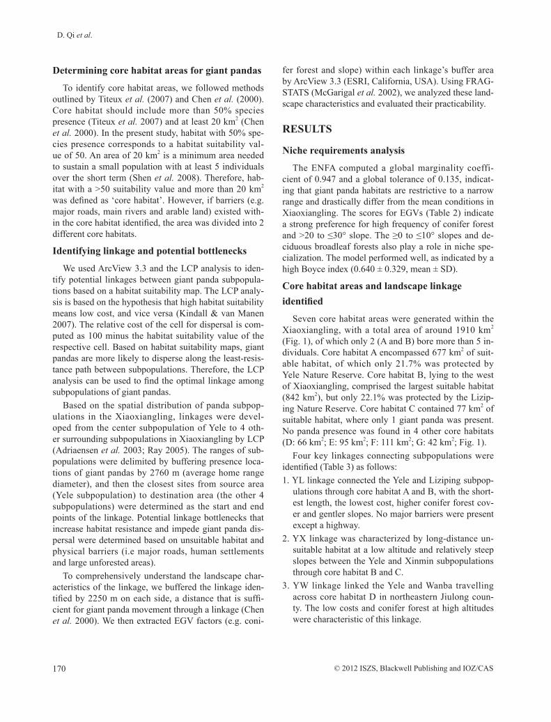
4. YM linkage connected the Yele with the Matou with a rather long path and many barriers.

DISCUSSIONLandscape patterns are very important in understand-

ing the effects of population subdivision on species sur-vival (Fahrig & Merriam 1994). Animal displacements are constrained by resistance of landscape components (Baguette & Van Dyck 2007), and would benefit from enhanced habitat linkages (Rayfield et al. 2010). For the isolated giant panda population in Xiaoxiangling, Zhu et al. (2010) suggest that gene flow would be enhanced if the connectivity between currently fragmented for-ests were increased. However, potential linkages based on ecological requirements between giant panda sub-populations have not been previously considered. This prompted us to examine how landscape features might affect giant panda dispersal and movement between sep-arated populations. Using a spatial habitat suitability model and LCP analysis, we quantified the habitat suit-ability and identified potential linkages among subpop-ulations of giant pandas in Xiaoxiangling. Our results highlight that a variety of landscape features might act as barriers for giant panda dispersal or movement, and provide suggestions for locations where conservation efforts can be focused. A total of 1910 km2 core habitat areas and 4 linkages are identified in the Xiaoxiangling mountains.

According to historical records, giant panda habitats in Xiaoxiangling were formerly continuous (Hu 2001). Due to the increase in human population and forest log-ging in this region over the past 3 centuries, especial-ly human explosion from 1662 to 1795, the panda pop-ulation experienced a demographic collapse (Zhu et al. 2010). Nowadays, a total of 32 giant pandas are divid-ed into 5 subpopulations, which arouses our concern about the survival of the isolated mountainous popula-tion. Among 5 subpopulations, 3 of them (Liziping, Yele and Xinmin) live in the core habitat areas. Liziping and Yele subpopulations in the core habitat A and B, respec-tively, lying to both sides of National Road 108, encom-pass large amounts of suitable habitat. However, human activity (i.e. a reservoir in Yele town) has placed great pressure on the Yele subpopulation. The Xinmin sub-population, comprising 1 individual, lives in core habitat C with enough suitable habitat. The Matou subpopula-tion, with only 19 km2 of suitable habitat, is surround-ed by anthropogenic barriers to dispersal. The Wanba subpopulation, near the core habitat D, might provide enough habitat for 2 individuals in this subpopulation. In addition, based on our habitat suitability map, core habitats E and F have potential values as habitat linkag-es across the region. With respect to these isolated sub-populations, Zhu et al. (2010) predict that demographic, genetic and environmental fluctuations will lead to ex-tinction of giant pandas in the Xiaoxiangling mountains in the future if these small subpopulations remain isolat-

Table 3 Characteristics of the 4 linkages identified by least-cost path analysis for the giant panda in the Xiaoxiangling mountains (YX: Yele-Xinming; YL: Yele-Liziping; YM: Yele-Matou; YW: Yele-Wanba).

Characteristics LinkageYX YL YM YW

Accumulated cost 2995.6 693.1 3166.6 1851.0Average habitat suitability (±SD) 44.7 ± 33.6 55.8 ± 29.6 41.4 ± 31.9 31.4 ± 29.3

Distance through core habitat area (km) 50.4 15.7 38.2 22.8Distance through below the 20 habitat suitability (km) 3.6 0.0 3.9 2.7Maximum length of below the 20 habitat suitability (km) 3.4 0.0 1.2 1.4Mean altitude (±SD) 2078 ± 951 2789 ± 586 3373 ± 679 3561 ± 645Mean slope (±SD) 31.0 ± 10.2 25.4 ± 10.3 29.5 ± 9.9 30.9 ± 9.8Number bottleneck through below 20 habitat suitability 2 0 13 2Percent of conifer forest (%) 35.8 39.4 31.4 31.0

Total length (km) 54.2 15.7 54.0 27.0


123456789

101112131415161718192021222324252627282930313233343536373839404142434445464748495051

D. Qi et al.

ed. Therefore, enhancing linkages that will facilitate gi-ant panda movement and colonization among these iso-lated subpopulations is urgent. Little is known about the details of giant panda dispersal. Pan et al. (2001) found that giant pandas moved approximately 30 km in sever-al months in the Qinling mountains. Hu et al. (2010) es-timate a mean dispersal distance of 12.5 km for giant pandas in the Liangshan mountains. Therefore, we sur-mise that these 4 linkages, ranging from 15 to 54 km in length, could very likely be used by giant pandas if the problem of barriers to dispersal were solved.

Although 2 protected areas are established, local eco-nomic development in the remaining forest is threaten-ing the function of the YL linkage. The linkage has been proposed for giant pandas by other researchers (Ran et al. 2004; Zhu et al. 2010), but no quantitative analy-ses regarding its feasibility have been undertaken. Due to habitat destruction and human activities, gene flow between individuals of Liziping and Yele subpopula-tions is severely inhibited (Zhu et al. 2010). In particu-lar, the National Road 108 bisects the linkage and pos-es a significant barrier to giant panda dispersal along the linkage. The newly constructed Chengdu–Xichang high-way facilitates human development and increases fur-ther isolation of this area. Although an underpass was incorporated into road construction, fragmentation and edge effects caused by this highway are likely, to some extent, to affect movement between the 2 subpopula-tions. Interestingly, during the field survey, we found a significant presence of giant pandas along this linkage, near the road, suggesting that giant pandas occasionally attempt to disperse. This also provides evidence of high predictive accuracy and the important conservation val-ue of this proposed linkage. Thus, it is imperative to en-hance the function of the YL linkage in order to protect the 2 largest subpopulations in Xiaoxiangling.

The Xinmin subpopulation lives in the C core habi-tat and few individuals remain. In terms of linking with the Yele subpopulation, the YX linkage is character-ized by low altitude, 3.4 km of unsuitable area and close proximity to human settlements (i.e. Xieluo town), all of which are significant barriers for panda dispersal. In 2009, 1 subadult female (named Luxin), rescued at the Xinlong town in Luding county, was found to be from the Xinmin subpopulation; however, her dispersing path was not in the YX linkage proposed. Because of habitat heterogeneity and the presence of barriers which affect panda dispersal direction (see Hu et al. 2010), we be-lieve that Xieluo town with low suitability habitat near the linkage might have impeded the dispersal of Luxin

along the direction towards Yele. Therefore, decreasing human impact along the YX linkage would facilitate the dispersal of the giant panda from Xinmin to Yele.

For the YW linkage connecting Yele with Wanba sub-populations, a 2.7 km of grassland cover along the link-age may be a barrier to dispersal. Another potential bar-rier for dispersing giant pandas is livestock grazing, which has become a major human disturbance in this area (Ran et al. 2004). Fortunately, the implementation of the Grain-to-Green Program in 1998 may be helpful for restoring and expanding panda habitat. Of the 4 pro-posed linkages, the YM linkage between Yele and Ma-tou subpopulations, appears the least likely to facilitate successful dispersal between subpopulations, because many anthropogenic barriers exist (i.e. historic forest logging, human settlements and cropland areas) along this linkage. Moreover, the impact of past forest logging on panda habitat will be felt for some years (Ran et al. 2004). As a Yi minority area, the low agricultural pro-ductivity and high human birth rate (i.e. a 3-child poli-cy) might have negative effects on panda habitat.

In conclusion, our results highlight the value of the ENFA and LCP for understanding patterns of suitable habitat and connectivity between habitats for giant pan-da subpopulations. Although Xiaoxiangling contains sufficiently large, suitable habitat for current subpopu-lations, it has been divided into 6 separated core habi-tat areas, which could affect the long-term survival of the giant panda. To ensure the long-term persistence of these subpopulations, the 4 potential linkages identi-fied should be enforced through effective management. Among the 4 linkages identified, the YL linkage is the most feasible and important to implement to enhance the movement of the 2 largest subpopulations. Identify-ing wild panda distributions outside protected areas is extremely difficult and costly for the governments and relevant organizations. Therefore, we suggest that the opportunities provided by the up-coming ‘Fourth Na-tional Survey of Giant Pandas’ should be capitalized on so as to monitor the species presence along the linkage areas described.

ACKNOWLEDGMENTSThis research was supported by the National Na-

ture Science Foundation (30830020), Key Program of Knowledge Innovation Program of Chinese Academy of Sciences (KSCX2-EW-Z-4) and the China Postdoctoral Science Foundation (200904501111).


123456789101112131415161718192021222324252627282930313233343536373839404142434445464748495051


REFERENCESAdriaensen F, Chardon JP, De Blust G et al. (2003). The

application of ‘least cost’ modelling as a function-al landscape model. Landscape and Urban Planning 64, 233–47.

Baguette M, Van Dyck H (2007). Landscape connec-tivity and animal behavior: functional grain as a key determinant for dispersal. Landscape Ecology 22, 1117–29.

Barrows CW, Fleming KD, Allen MF (2011). Identify-ing habitat linkage to maintain connectivity for cor-ridor dwellers in fragmented landscape. Journal of Wildlife Management 75, 682–91.

Caughley G (1994). Directions in conservation biology. Journal of Animal Ecology 63, 215–44.

Chen LD, Fu BJ, Liu XH (2000). Landscape pattern de-Landscape pattern de-sign and wildlife conservation in nature reserve – a case study of Wolong Nature Reserve. Journal of Natural Resources 15, 164–9 (In Chinese).

Chetkiewicz C-LB, Boyce MS (2009). Use of resource selection functions to identify conservation corridors. Journal of Applied Ecology 46, 1036–47.

Chetkiewicz C-LB, St. Clair CC, Boyce MS (2006). Corridors for conservation: integrating pattern and process. Annual Review of Ecology, Evolution, and Systematics 37, 317–42.

Engler R, Guisan A, Rechsteiner L (2004). An improved approach for predicting the distribution of rare and endangered species from occurrence and pseudo-absence data. Journal of Applied Ecology 41, 263–74.

Fahrig L, Merriam G (1994). Conservation of fragment-ed populations. Conservation Biology 8, 50–59.

Fahrig L (2003). Effects of habitat fragmentation on bio-diversity. Annual Review of Ecology Evolution, and Systematics 34, 487–515.

Harrison S, Bruna E (1999). Habitat fragmentation and large-scale conservation: what do we know for sure? Ecography 22, 225–32.

Hirzel AH, Arlettaz R (2003). Modeling habitat suit-ability for complex species distributions by the envi-ronmental-distance geometric mean. Environmental Management 32, 614–23.

Hirzel AH, Hausser J, Chessel D, Perrin N (2002). Eco-logical-niche factor analysis: how to compute habitat suitability maps without absence data? Ecology 83, 2027–36.

Hirzel A, Hausser J, Perrin N (2007). Biomapper 4.0. [Cited 16 November 2008.] Available from URL: http://www.unil.ch/biomapper

Hirzel AH, Le Lay G, Helfer V, Randin C, Guisan A (2006). Evaluating the ability of habitat suitability models to predict species presences. Ecological Mod-elling 199, 142–52.

Hirzel AH, Posse B, Oggier P-A, Crettenand Y, Glenz C, Arlettaz R (2004). Ecological requirements of rein-troduced species and the implications for release pol-icy: the case of the bearded vulture. Journal of Ap-plied Ecology 41, 1103–16.

Hu JC, Schaller GB, Pan WS, Zhu J (1985). The Giant Pandas of Wolong. Sichuan Publishing House of Sci-ence and Technology Press, Chengdu (In Chinese).

Hu YB, Zhan XJ, Qi DW, Wei FW (2010). Spatial ge-netic structure and dispersal of giant pandas on a mountain-range scale. Conservation Genetics 11, 2145–55.

Husté A, Boulinier T (2007). Determinants of local ex-tinction and turnover rates in urban bird communi-ties. Ecological Applications 17, 168–80.

Jackson DA (1993). Stopping rules in principal compo-nents analysis: a comparison of heuristical and statis-tical approaches. Ecology 74, 2204–14.

Kindall JL, van Manen FT (2007). Identifying habitat linkages for American black bears in North Carolina, USA. Journal of Wildlife Management 71, 487–95.

Larkin JL, Maehr DS, Hoctor TS, Orlando MA, Whit-ney K (2004). Landscape linkages and conservation planning for the black bear in west-central Florida. Animal Conservation 7, 23–34.

Leica Geosystems GIS and Mapping (2003). Erdas Imagine 8.7 Field Guide, Leica Geosystems GIS and Mapping LLC, Atlanta, GA.

McGarigal K, Cushman SA, Neel MC, Ene E (2002). FRAGSTATS: Spatial Pattern Analysis Program for Categorical Maps. [Cited 11 July 2007.] Available from URL: http://www.umass.edu/landeco/research/fragstats/fragstats.html

Pan WS, Lü Z, Zhu XJ et al. (2001). A Chance for Last-ing Survival. Peking University Press, Beijing (In Chinese).

Qi DW, Hu YB, Gu XD, Li M, Wei FW (2009). Ecolog-ical niche modeling of the sympatric giant and red pandas on a mountain range scale. Biodiversity and Conservation 18, 2127–41.


123456789

101112131415161718192021222324252627282930313233343536373839404142434445464748495051

D. Qi et al.

Ran JH, Liu SY, Wang HJ, Zeng ZY, Sun ZY, Liu SC (2004). A survey of disturbance of giant panda habi-tat in the Xiaoxiangling Mountains of Sichuan prov-ince. Acta Theriologica Sinica 24, 277–81.

Ray N (2005). PATHMATRIX: a geographical infor-mation system tool to compute effective distances among samples. Molecular Ecology Notes 5, 177–80.

Rayfield B, Fortin M-J, Fall A (2010). The sensitivity of least-cost habitat graphs to relative cost surface val-ues. Landscape Ecology 25, 519–32.

Sattler T, Bontadina F, Hirzel AH, Arlettaz R (2007). Ecological niche modeling of 2 cryptic bat species calls for a reassessment of their conservation status. Journal of Applied Ecology 44, 1188–99.

Schaller GB, Hu JC, Pan WS, Zhu J (1985). The Giant Pandas of Wolong. The University of Chicago Press, Chicago.

Shen GZ, Feng CY, Xie ZQ, Ouyang ZY, Li JQ, Pascal M (2008). Proposed conservation landscape for giant pandas in the Minshan Mountains, China. Conserva-tion Biology 22, 1144–53.

State Forestry Administration of China (SFA) (2006) . The Third National Survey Report on the Giant Pan-da in China. Chinese Science and Technology Pub-lishing House, Beijing (In Chinese).

Swaisgood RR, Wei F, McShea WJ, Wildt DE, Kouba AJ, Zhang Z (2011). Can science save the giant pan-da? Unifying science and policy in an adaptive man-agement paradigm. Integrative Zoology 6, 290–96.

Titeux N, Dufrene M, Radoux J et al. (2007). Fitness-related parameters improve presence only distribu-tion modeling for conservation practice: the case of the red-backed shrike. Biological Conservation 138, 207–23.

Wang TJ, Ye XP, Skidmore AK, Toxopeus AG (2010). Characterizing the spatial distribution of giant panda (Ailuropoda melanoleuca) in fragmented forest land-scapes. Journal of Biogeography 37, 865–78.

Wilcox BA, Murphy DD (1985). Conservation strategy: the effects of fragmentation on extinction. The Amer-ican Naturalist 125, 879–87.

Zhang BW, Li M, Zhang ZJ et al. (2007). Genetic via-bility and population history of the giant panda, put-ting an end to the ‘evolutionary dead end’? Molecu-lar Biology and Evolution 24, 1801–10.

Zhang ZJ, Swaisgood RR, Zhang SN et al. (2011). Old-growth forest is what giant pandas really need. Biolo-gy Letters, doi: 10.1098/rsbl.2010.1081

Zhu LF, Zhan XJ, Wu H et al. (2010). Conservation im-plications of drastic reductions in the smallest and most isolated populations of giant pandas. Conserva-tion Biology 24, 1299–304.

Zhu LF, Zhang SN, Gu XD, Wei FW (2011). Significant genetic boundaries and spatial dynamics of giant pan-das occupying fragmented habitat across southwest China. Molecular Ecology 20, 1122–32.

Documents

Quantifying landscape linkages among giant panda subpopulations in regional scale conservation