Quantification of th e fine -scale distribution of Mn ... · A strong influence of mean backscatter, fine scale BPI ... 72 1996) , showed that the ... 134 (obtained by

1

Quantification of the fine-scale distribution of Mn-nodules: insights 1

from AUV multi-beam and optical imagery data fusion 2

3

4

Evangelos Alevizos1, Timm Schoening1, Kevin Koeser1, Mirjam Snellen2,3, Jens Greinert1 5

6 1 GEOMAR Helmholtz Center for Ocean Research, 24148 Kiel, Germany 7 2Acoustics Group, Faculty of Aerospace Engineering, Delft University of Technology, 8

Kluyverweg 1, 2629 HS Delft, the Netherlands 9 3Deltares, Princetonlaan 6, 3584 CB Utrecht, the Netherlands 10

11

Abstract. Autonomous underwater vehicles (AUVs) offer unique possibilities for exploring the 12

deep seafloor in high resolution over large areas. We highlight the results from AUV-based 13

multibeam echosounder (MBES) bathymetry / backscatter and digital optical imagery from the 14

DISCOL area acquired during research cruise SO242 in 2015. AUV bathymetry reveals a 15

morphologically complex seafloor with rough terrain in seamount areas and low-relief 16

variations in sedimentary abyssal plains which are covered in Mn-nodules. Backscatter 17

provides valuable information about the seafloor type and particularly about the influence of 18

Mn-nodules on the response of the transmitted acoustic signal. Primarily, Mn-nodule 19

abundances were determined by means of automated nodule detection on AUV seafloor 20

imagery and nodule metrics such as nodules m-2 were calculated automatically for each image 21

allowing further spatial analysis within GIS in conjunction with the acoustic data. AUV-based 22

backscatter was clustered using both raw data and corrected backscatter mosaics. 23

In total, two unsupervised methods and one machine learning approach were utilized for 24

backscatter classification and Mn-nodule predictive mapping. Bayesian statistical analysis was 25

applied to the raw backscatter values resulting in six acoustic classes. In addition, Iterative Self-26

Organizing Data Analysis (ISODATA) clustering was applied to the backscatter mosaic and its 27

statistics (mean, mode, 10th, and 90th quantiles) suggesting an optimum of six clusters as well. 28

Part of the nodule metrics data was combined with bathymetry, bathymetric derivatives and 29

backscatter statistics for predictive mapping of the Mn-nodule density using a Random Forest 30

classifier. Results indicate that acoustic classes, predictions from Random Forest model and 31

image-based nodule metrics show very similar spatial distribution patterns with acoustic 32

classes hence capturing most of the fine-scale Mn-nodule variability. Backscatter classes reflect 33

areas with homogeneous nodule density. A strong influence of mean backscatter, fine scale BPI 34

and concavity of the bathymetry on nodule prediction is seen. These observations imply that 35

nodule densities are generally affected by local micro-bathymetry in a way that is not yet fully 36

understood. However, it can be concluded that the spatial occurrence of Mn-covered areas can 37

be sufficiently analysed by means of acoustic classification and multivariate predictive 38

mapping allowing to determine the spatial nodule density in a much more robust way than 39

previously possible. 40

Biogeosciences Discuss., https://doi.org/10.5194/bg-2018-60Manuscript under review for journal BiogeosciencesDiscussion started: 15 February 2018c© Author(s) 2018. CC BY 4.0 License.

2

41

1. Introduction 42

1.1 Mn-nodules exploration 43

44

Research on Mn-nodules received increased attention in the last decade due to increasing 45

prices for ores rich in Cu, Ni or Co, i.e. metal resources that are contained in Mn-nodules. In 46

nature, the largest Mn-nodule occurrences are found in the deep sea, e.g. the equatorial 47

Pacific between the Clarion and Clipperton fracture zone (CCZ), the Peru Basin as well as the 48

Atlantic and Indian Ocean (Petersen et al., 2016 ). In the typically muddy sediments of the 49

deep sea, Mn-nodules form an important hard substrate providing a habitat for deep sea 50

sessile fauna such as sponges, corals and associated organisms (Vanreussel et al., 2016; Purser 51

et al., 2016). Therefore, mapping Mn-nodule fields is a two-fold task, comprising not only the 52

assessment of Mn-nodules and their density distribution for accurate resource assessment, 53

but also the improved understanding of the natural habitat heterogeneity and its relation to 54

the deep sea ecology. Knowledge about Mn-nodule habitats will support mitigation strategies 55

for mining-induced impacts. Since an increasing number of countries move forward with 56

exploitation plans for Mn-nodules in the CCZ, strategies for a detailed mapping of the deep sea 57

Mn-nodule fields might become mandatory in order to proceed with licensing procedures 58

prior to any mining activity. 59

Deep sea mining will cause substantial disturbances of the deep sea ecosystem since Mn-60

nodules, the primary hard substrate, will be removed and massive re-sedimentation of the top 61

20 to 30cm of sediment of the mined area will occur (Bluhm et al., 1995, Vanreussel et al., 62

2016).Thus, efforts have been made to investigate the effects of potential mining disturbances 63

in the past (e.g. Thiel et al., 2001) and currently during the project “Ecological Aspects of Deep 64

Sea Mining” as part of the Joint Programming Initiative Healthy and Productive Seas and 65

Oceans (JPI Oceans). To study in detail the potential effects of a deep sea disturbance by Mn-66

nodule mining to benthic fauna, a plough-experiment was performed in 1989 in the Peru Basin 67

as part of the DISturbance and reCOLonization project (DISCOL, www.discol.de). A plough of 68

8m width was towed 78 times over a 2nmi wide circular area (February-March 1989) to 69

generate dense and less dense impact sub-areas. Photographic surveys, sediment and 70

biological sampling before and after the disturbance (September 1989, March 1992, February 71

1996), showed that the plough marks were well visible even after 26 years and that the 72

benthic fauna did not recover to its initial state. The data used in this study were collected 73

during the SO242-1 cruise to the DISCOL area during summer 2015, 26 years after the DSICOL 74

experiment. 75

76

1.2 The DISCOL study area 77

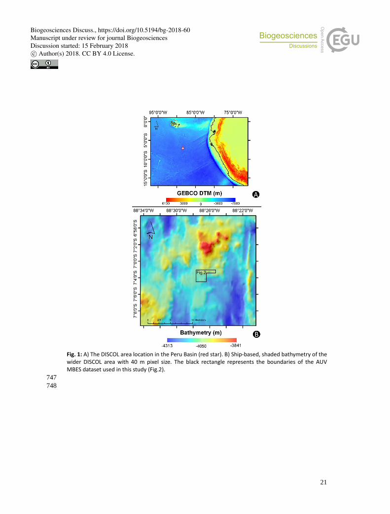
The DISCOL working area is situated 560 nmi SW of Guayaquil on the Pacific Oceanic 78

Plate in the Peru Basin (Fig. 1A) in about 4150 m water depth. The larger DISCOL area ranges 79

from 3800m to 4300m water depth (Fig. 1B) and is characterized by N-S oriented graben and 80

horst structures with a deep N-S elongated basin with water depths down to 4300m. An 11 km 81

wide seamount complex in the NE along with a second seamount complex to the SW and three 82


3

higher mounds to the NW clearly show that the DISCOL area is not located on a flat and 83

homogenous deep seafloor. 84

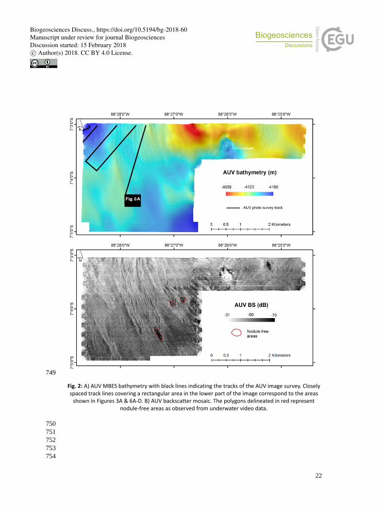
The ploughed DISCOL Experimental Area (DEA) itself is located on a relatively smooth, 85

slightly elevated part of the seafloor with a central valley of about 20m depth that dips 86

southward (Fig. 2A). When inspecting the bathymetry data generated by the autonomous 87

underwater vehicle (AUV) in more detail, the central part of the area shows a 20m deep valley, 88

the floor of which is comprised by low-relief N-S trending ridges giving the impression of a 89

braided river system (Fig. 2A). Despite the rich morphological features in the study area, it 90

does not contain steep slopes and represents a rather smooth seafloor (<5 degrees). 91

92

93

1.3 Acoustic mapping of Mn-nodules and study objectives 94

Acoustic mapping has proved to be a useful tool for supporting deep sea mineral 95

resource assessments. The initial studies mentioned below, showed promising results for Mn-96

nodule detection and quantification, however, progress in more detailed and meaningful 97

method development and data processing capabilities has remained slow, mainly due to 98

fluctuations in the global interest of deep sea mining. The majority of surveys performed for 99

Mn-nodule mapping purposes rely on acoustic remote sensing and near-bottom photography 100

(de Moustier, 1985). The applicability of acoustic methods is based on the clear acoustic 101

contrast of at least 11 dB between the background deep sea soft sediment and the nodules (de 102

Moustier 1985). Weydert (1985) found that the nodule size is proportional to the average 103

backscatter strength for low frequency signals (<30 kHz). In addition, Weydert (1990) 104

concluded that it is possible to map the percentage of seafloor covered by nodules based on 105

backscatter measurements of sonar frequencies higher than 30 kHz , whereas for a frequency 106

of 9 kHz it is possible to use the backscatter response to determine whether the nodule 107

diameter is greater than 6 cm or smaller than 4 cm. Masson and Scanlon (1993) suggested that 108

lower sonar frequencies produce a much weaker acoustic contrast between nodules and 109

surrounding sediments for nodules of given size. They concluded that on a seafloor covered 110

with mixed-size nodules larger nodules will have a greater impact on the backscattered energy 111

than smaller ones. They also suggested that minor differences of nodule coverage will have a 112

considerable effect in backscatter values. A more recent study by Chakrabotry et al. (1996) 113

suggested that the nodule coverage is proportional to the backscatter strength and that for 114

low frequency (15 kHz; wavelength ca. 10 cm) the main type of scattering is Rayleigh scattering 115

(wavelength/10 < nodule size) for nodules and coherent scattering for fine sediments. 116

During one of the first deep sea studies for acoustic mapping of Mn-nodules, de Moustier 117

(1985) utilized a multi-beam echo-sounder (MBES) sonar combined with near-bottom acoustic 118

measurements and photographs from a deep towed camera system to infer nodule coverage. 119

He managed to obtain high agreement between relative backscatter intensity classes and 120

three types of nodule coverage as interpreted from seafloor imagery (dense, intermediate and 121

bare). At that time, his results highlighted the great potential of MBES technology in deep sea 122

mineral prospecting. In more recent years Lee and Kim (2004) utilized side-scan sonar (SSS) to 123

examine the relation of regional nodule abundance with geomorphology. According to their 124


4

qualitative analysis, lower backscatter values are related with abyssal troughs whereas 125

increased backscatter values are related to abyssal hills. Additionally, Ko et al. (2006) 126

attempted to examine the relation between MBES bathymetry and slope with nodule density 127

in the equatorial Pacific without identifying a solid pattern. Most recently, Okazaki and Tsune 128

(2013) utilized AUV-based MBES, SSS and image data for Mn-nodule abundance assessment 129

and its relation to deep sea micro-topography. 130

More recent projects regarding resource assessment of Mn-nodules at large scales (0.1’ by 0.1’ 131

grid cell size) have been based on various spatial modelling and decision making techniques 132

(ISA, 2010). Most commonly, the kriging method has been applied on sparse ground truth data 133

(obtained by physical box-corer sampling) while logistic regression and fuzzy logic algorithms 134

were applied in multivariate data sets of Mn-nodule-related environmental variables such as 135

sediment type, sea surface chlorophyll and Ca Compensation Depth (CCD) (Agterberg & 136

Bohnam-Carter, 1999, Carranza & Hale, 2001). 137

In this study we analyse AUV-based MBES and image data for quantitative mapping of Mn-138

nodule densities in the Peru Basin. Particularly, we utilize local ground-truth information (Mn-139

nodule measurements from AUV photographs) in order to investigate a) its relation to acoustic 140

classification maps and b) its potential use for predictive mapping of Mn-nodules in wider 141

areas where only hydro-acoustic information is available. Therefore, we apply two 142

unsupervised methods (Bayesian probability and ISODATA) for seafloor acoustic classification 143

and a machine learning algorithm (Random Forest) for Mn-nodule density predictions beyond 144

the areas that were optically imaged using the AUV. 145

By applying different algorithms for unsupervised classification, we aim at comparing their 146

results against quantitative ground truth data of nodule metrics from automated analyses on 147

AUV imagery. This way, we will assess the ability of classification methods in discriminating 148

areas with distinct nodule densities. To our knowledge, this is the first time the Random Forest 149

algorithm is applied for predictive mapping of Mn-nodule densities. Therefore, we examine its 150

performance and the influence of various AUV MBES data on the Mn-nodule prediction 151

results. 152

153

154

2. Methodology 155

2.1 AUV MBES data acquisition and processing 156

The data in this study were collected using the AUV “Abyss” (built by HYDROID Inc.) from 157

GEOMAR, during cruise SO242-1 where various AUV missions were flown. The AUV is 158

equipped with a RESON Seabat 7125 MBES sensor with 200 kHz operating frequency, 256 159

beams with 1 by 2 degree opening angle along and across track, respectively. From the original 160

PDS2000 sonar data, files backscatter snippet data were extracted into s7k format whereas 161

bathymetry data were extracted into GSF format. Prior to exporting, MBES bathymetric data 162

were filtered within the PDS2000 software. Bathymetry data from different AUV dive-missions 163

were jointly used for interpolating one single grid of bathymetry and backscatter (Fig.2). 164

Latency and roll-related artefacts affected bathymetry in places due to a none-constant time 165

delay for roll values creating uncorrectable artefacts in the resulting grid. Therefore, the 166


5

bathymetry was smoothed by applying a Gaussian filter with a 10 m x 10 m rectangular 167

window with 3 and 5 standard deviations as smoothing factors in SAGA GIS. Filtered 168

bathymetry was visually inspected for artefacts using the hill-shade function in SAGA GIS, 169

giving satisfactory results. Vertical differences between the smoothed grid with the originally 170

processed surface were everywhere less than 1 m, highlighting that the filtering did not cause 171

significant smoothing and removal of finer details. The filtered bathymetric grid was used for 172

calculating a variety of derivatives listed in Table 2. 173

The MBES backscatter data were processed in two ways. First, the s7k/GSF pairs were 174

automatically corrected (for radiometric and geometric bias) and mosaicked in QPS FMGT (Fig. 175

2B). In addition, backscatter mosaic statistics were calculated and exported as GEOTIF files 176

using a 10 m x 10 m neighbourhood. The raw snippets data were exported prior to any 177

processing using a combination of in-house conversion software and QPS DMagic for merging 178

beam data with ray-traced easting and northing. The raw snippets data were transformed from 179

16-bit amplitude units to dB using the formula in Eq. (1): 180

181

Backscatter (dB) = 20*log10(amplitude) (1) 182 183

184

Raw backscatter data were processed by applying the Bayesian approach on certain beams as 185

described in Alevizos et al. (2015 and 2017) whereas the gridded data were analysed with 186

Random Forest (RF) regression trees and ISODATA clustering (see section below). An overview 187

of the software used to process and classify each type of dataset is presented in Table 1. 188

189

190

2.2 Seafloor imagery and automated image analysis 191

192

AUV surveys were undertaken for collecting close-up images from the seafloor using a camera 193

system recently described by Kwasnitschka et al (2016). In this system the camera is mounted 194

behind a dome port along with a 15mm fish-eye lens that produces extreme wide-angle 195

images. This type of lens and dome port configuration induces significant distortions to the 196

image which need to be corrected prior to any image analysis processing. Surveying at 197

altitudes of 4-8m above the seafloor and using the novel state-of the-art LED flash system, the 198

AUV collected several hundred-thousand seafloor images at a 1Hz interval. The respective AUV 199

surveys were designed to cover a large part of the study area with a single-track dive pattern 200

and also to focus on two selected areas running track lines 5m apart for dense 2D image 201

mosaicking (Fig. 2A). Each image was individually georeferenced using the AUV navigation and 202

altitude data. This way, each pixel of the AUV imagery is translated to an actual portion of the 203

seafloor. 204

For the automated image analyses (e.g. Mn-nodule counting), all images were smoothed by a 205

Gaussian filter to remove noise and then converted to grayscale for computational speedup. 206

Following, the images were corrected for inconsistent illumination due to the varying AUV 207

altitude using the fSpice method described by Schoening, et al. (2012). The central (sharpest, 208

best illuminated) region of each image was cropped and thresholded by an automatically 209


6

tuned intensity limit before contours in the resulting binary images were detected and fused to 210

blobs of pixels that served as nodule candidates. Each nodule candidate was finally fitted with 211

an ellipsoid to account for potentially buried parts of the nodule. The sizes of these ellipsoids 212

constitute the nodule size distribution within one image from which descriptive parameters 213

were derived. This kind of automated image processing resulted in quantitative information 214

such as: image area (square meters), number of nodules (n), percentage of seafloor covered by 215

nodules (amount of nodule pixels divided by total amount of image pixels), and the threshold 216

sizes (estimated 2D surface) of 1, 25, 50, 75 and 99 percent quantiles of the nodule size 217

distribution (comparable to a particle size analysis). A detailed publication on the nodule 218

delineation algorithm can be found in Schoenning et al. (2017), while the source code is 219

available online as Open Source (https://doi.pangaea.de/10.1594/PANGAEA.875070) 220

In this study, we considered the number of Mn-nodules per square meter as a normalized 221

measure of nodule density in order to avoid overestimation of Mn-nodules due to multiple-222

detections between overlapping images. This metric is derived from the ratio of the number of 223

nodules detected to the area (m2) of the image footprint (the size of the central ‘good’ part of 224

the image). Therefore the results of the predictive mapping are presented with 6 m x 6 m 225

resolution which is representative for the majority of image footprint sizes. 226

227

228

2.3 Seafloor classification and prediction methods 229

230

Three different approaches were applied for a predictive Mn-nodule mapping. The first 231

approach is an unsupervised method based on Bayesian statistics applied on raw snippet data. 232

It examines the within-beam backscatter variability in the entire area in order to estimate the 233

optimum number of seafloor classes. The output acoustic classes can then be validated with 234

available ground-truth data. The second approach, is based on the ISODATA algorithm (an 235

unsupervised method as well), applied on gridded backscatter data. This algorithm can 236

automatically adapt the number of classes to the data for given minimum and maximum 237

values set by the user. Finally, a supervised machine learning method was applied on gridded 238

bathymetric and backscatter data. This method requires a training set in order to model the 239

complex relationship between the Mn-nodules occurrences and the bathymetry, bathymetric 240

derivatives and backscatter information. The algorithm outputs a prediction grid for Mn-241

nodule densities and also estimates the importance of each input variable in accurately 242

predicting Mn-nodule densities. 243

244

245

246

247

248

249

250

251


7

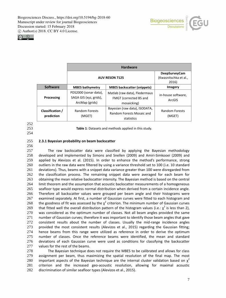
Hardware

AUV RESON 7125 DeepSurveyCam

(Kwasnitschka et al., 2016)

Software MBES bathymetry MBES backscatter (snippets) Imagery

Processing

PDS2000 (sonar data),

SAGA GIS (xyz, grids),

ArcMap (grids)

Matlab (raw data), Fledermaus

FMGT (corrected BS and

mosaicking)

in-house software,

ArcGIS

Classification /

prediction

Random Forests

(MGET)

Bayesian (raw data), ISODATA,

Random Forests Mosaic and

statistics

Random Forests

(MGET)

252 Table 1: Datasets and methods applied in this study. 253

254

2.3.1 Bayesian probability on beam backscatter 255

256

The raw backscatter data were classified by applying the Bayesian methodology 257

developed and implemented by Simons and Snellen (2009) and Amiri-Simkooei (2009) and 258

applied by Alevizos et al. (2015). In order to enhance the method’s performance, strong 259

outliers in the raw data were filtered by using a variance threshold set to 100 (i.e. 10 standard 260

deviations). Thus, beams with a snippet data variance greater than 100 were disregarded from 261

the classification process. The remaining snippet data were averaged for each beam for 262

obtaining the mean relative backscatter intensity. The Bayesian method is based on the central 263

limit theorem and the assumption that acoustic backscatter measurements of a homogeneous 264

seafloor type would express normal distribution when derived from a certain incidence angle. 265

Therefore all backscatter values were grouped per beam angle and their histograms were 266

examined separately. At first, a number of Gaussian curves were fitted to each histogram and 267

the goodness of fit was assessed by the χ2 criterion. The minimum number of Gaussian curves 268

that fitted well the overall distribution pattern of the histogram values (i.e.: χ2 is less than 2), 269

was considered as the optimum number of classes. Not all beam angles provided the same 270

number of Gaussian curves; therefore it was important to identify those beam angles that gave 271

consistent results about the number of classes. Usually the mid-range incidence angles 272

provided the most consistent results (Alevizos et al., 2015) regarding the Gaussian fitting; 273

hence beams from this range were utilized as reference in order to derive the optimum 274

number of classes. Once the reference beams were identified, the mean and standard 275

deviations of each Gaussian curve were used as conditions for classifying the backscatter 276

values for the rest of the beams. 277

The Bayesian technique does not require the MBES to be calibrated and allows for class 278

assignment per beam, thus maximizing the spatial resolution of the final map. The most 279

important aspects of the Bayesian technique are the internal cluster validation based on χ2 280

criterion and the increased geo-acoustic resolution, allowing for maximal acoustic 281

discrimination of similar seafloor types (Alevizos et al., 2015). 282


8

2.3.2 ISODATA classification for grids 283

284

The ISODATA classification was applied to the backscatter mosaic and its derived 285

statistics (Table 2) using the ISODATA algorithm implemented in SAGA GIS. ISODATA stands for 286

Iterative Self-Organizing Data Analysis and has been applied in several marine mapping studies 287

involving backscatter information (Diaz, 1999; Hühnerbach et al., 2008; Blondel and Gomez-288

Sichi 2009). The fundamentals of ISODATA processing are described in detail by Dunn (1977) 289

and Memarsadeghi et al. (2007). A particular advantage of this method apart from its fast 290

execution is that it estimates a suitable number of classes by dividing clusters with large 291

standard deviations and by merging similar clusters at the same time (Diaz 1999). This is done 292

automatically and the user only defines an empirical minimum and maximum number of 293

classes. 294

295

2.3.3 Random Forest predictive mapping for grids 296

297

To exploit the full range of MBES gridded data and for comparison purposes, supervised 298

classification was applied to the bathymetry, bathymetric derivatives and backscatter statistics 299

(Table 2). Applying a machine learning algorithm was encouraged due to the abundant ground-300

truth data (nodule metrics from automated image analysis) and the high resolution of the 301

various MBES layers. The Random Forest algorithm as implemented in the MGET toolbox for 302

ArcGIS was used (http://mgel2011-kvm.env.duke.edu/mget). Initially developed by Breiman 303

(2001) it has shown good results in marine predictive habitat mapping (Stephens and Diesing 304

2014, Lucieer et al., 2013, Che-Hasan et al., 2014). The algorithm requires a training data set 305

with the response variable (here: nodule density from AUV imagery analysis results) and a set 306

of explanatory variables (here: bathymetry, bathymetric derivatives, backscatter) as inputs in 307

order to model the relationship between them. The training set provides the required 308

“knowledge” about the response variable and its corresponding explanatory variable’s values. 309

At the next stage, an ensemble procedure based on several regression trees of random subsets 310

of the explanatory variables is iteratively applied for classifying/predicting Mn-nodule density 311

per grid-cell using a-priori information from the training sample. The prediction at a certain 312

grid-cell is defined by the majority votes of all random subsets of trees (Gislason et al., 2006). 313

During the iterative processing, the Random Forest will reserve randomly selected parts of the 314

training sample for internal cross-validation of the results (out-of-bag sample). During each 315

iteration, one explanatory variable is neglected and its importance score is calculated 316

according to its contribution to the resulting prediction error. The variable importance 317

calculation is considered one of the main advantages of the Random Forest algorithm. An 318

important step prior to Random Forest application is data exploration. With data exploration it 319

is possible to identify which explanatory variables are capable to discriminate patterns of 320

nodule density in the study area better. A standard approach is to explore the probability 321

density function of the response variable with each of the other gridded variables (e.g. slope, 322

BPI, etc.). These plots give first indications about the distribution type of the response variable 323

for a given explanatory variable. 324


9

The explanatory variables presented in Table 2 were chosen as good descriptors of nodule 325

density in the area based on the probability density functions of arbitrarily chosen classes of 326

nodule density (Fig. A1, Appendix). The arbitrary classes where based on the quantiles method 327

for classifying the nodule density histogram. It has to be noted that the arbitrary classes were 328

used only for data exploration and not for the prediction of nodule densities. All descriptor-329

grids were resampled to 6 m x 6 m pixels in order to be compatible with the average effective 330

area of the AUV images upon which nodule metrics were computed. 331

An appropriate selection of training samples is fundamental for modelling the relationship 332

between the response variable and the gridded descriptor data. Particularly, the training 333

samples need to span the entire range of the study area capturing most of the data variability. 334

They have to contain as diverse values as possible regarding both the nodule density and the 335

corresponding gridded descriptor data. 336

337

338

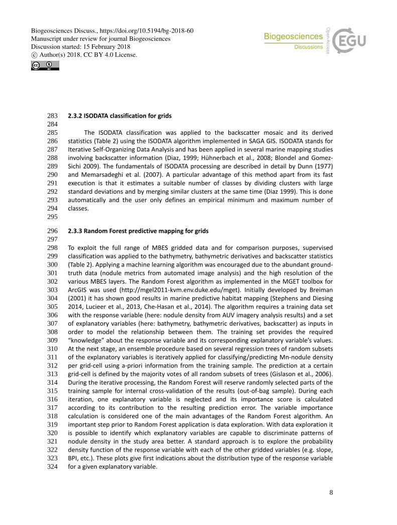
Explanatory variables

Description

From bathymetry Scale: 6 m cell size

Depth AUV MBES, smoothed with Gaussian filter (5σ)

Slope ArcGIS slope algorithm in percent units

BPI

Relative position of pixels compared to their neighbors. Inner radius 10m, outer radius 100 m

(Iwashahi and Pike, 2007) SAGA GIS terrain analysis toolbox

LS factor The integrated slope length and inclination, formula from Moore et al. (1991), SAGA GIS terrain analysis

toolbox

Terrain Ruggedness Index (TRI)

Measure of the irregularity of a surface in 5m radius neighborhood (Iwashahi and Pike, 2007), SAGA GIS

terrain analysis toolbox

Concavity Measure of negative curvature of a surface (Iwashahi

and Pike, 2007), SAGA GIS terrain analysis toolbox

From backscatter Scale: 10x10 m neighborhood, 6 m cell size

mean Average dB value of pixels falling within the

neighborhood (FMGT module)

mode Most frequent dB value of pixels falling within the

neighborhood (FMGT module)

10% quantile Value of neighborhood pixels describing the lower

10% of the total dB distribution (FMGT module)

90% quantile Value of neighborhood pixels describing the 90% of

the total dB distribution (FMGT module)

Table 2: Description of MBES features (bathymetric derivatives and backscatter statistics) that are used 339 as explanatory variables in random forests predictions. 340

341

342

343


10

3. Results 344

3.1 Automated nodule detection from AUV images 345

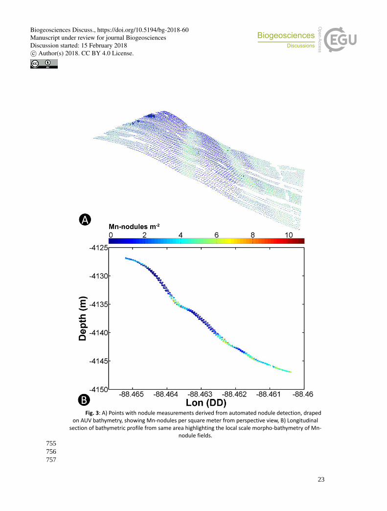
The automated nodule detection algorithm results for nodule density (number of nodules m-2) 346

are shown in Fig. 3. The dense point cloud offers a detailed view of the nodule spatial 347

distribution which can significantly enhance the interpretation of nodule density in 348

conjunction with MBES bathymetry. In Fig. 3 the nodule density fluctuates in a pattern of 349

alternating bands. By colorizing the seafloor surface and the bathymetric profile cross-section 350

according to nodule density values, it can be seen that higher nodule densities appear on 351

smooth slope features where the seafloor appears locally concave or terraced and also on the 352

foot of these slopes which appear relatively lower compared to the surrounding area. By 353

colouring the AUV bathymetry according to the nodule density it became clear that MBES 354

derivatives may be useful for quantifying the nodule distribution in the entire study area. We 355

thus calculated bathymetric derivatives such as BPI, concavity, slope and slope-related 356

derivatives (LS factor, TRI) to be included in predicting nodule densities. 357

358

3.2 Bayesian acoustic classification of raw BS data 359

360

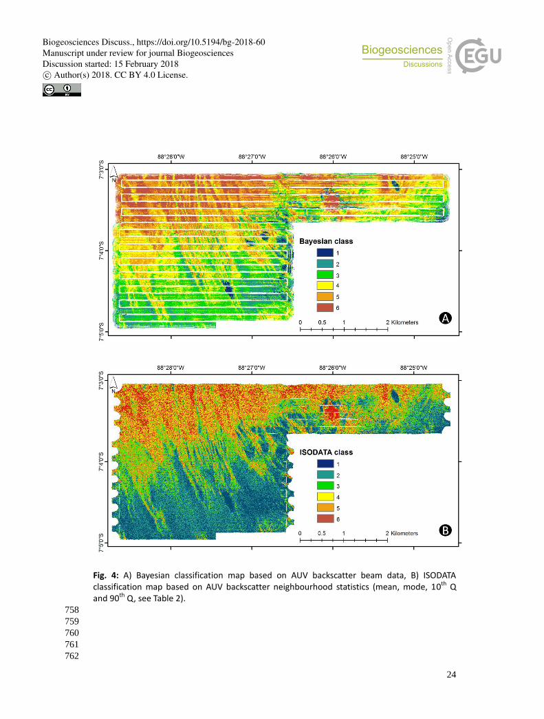
The Bayesian method identified six classes based on the analysis of beams with incidence 361

angles between 38 and 42 degrees (Table 3). Despite the variance-based filtering, it was not 362

possible to compensate for the remaining effects on beam incidence angles in the middle 363

range and towards the nadir. We believe that these effects are responsible for the stripe-like 364

classification at the outer part of the swath. The selection of six classes resulted from the 365

agreement between two adjacent beams (Table 3) and the relative lower overlap of the 366

Gaussian curves. The finally derived classes are ordinal; meaning that from class 1 to class 6 367

there is an increase in backscatter intensity. The spatial distribution of the acoustic classes 368

expresses a gradient of high to low backscatter classes in the N-S direction (Fig. 4A). The 369

nodule-free areas holding lowest backscatter values are captured clearly. 370

371

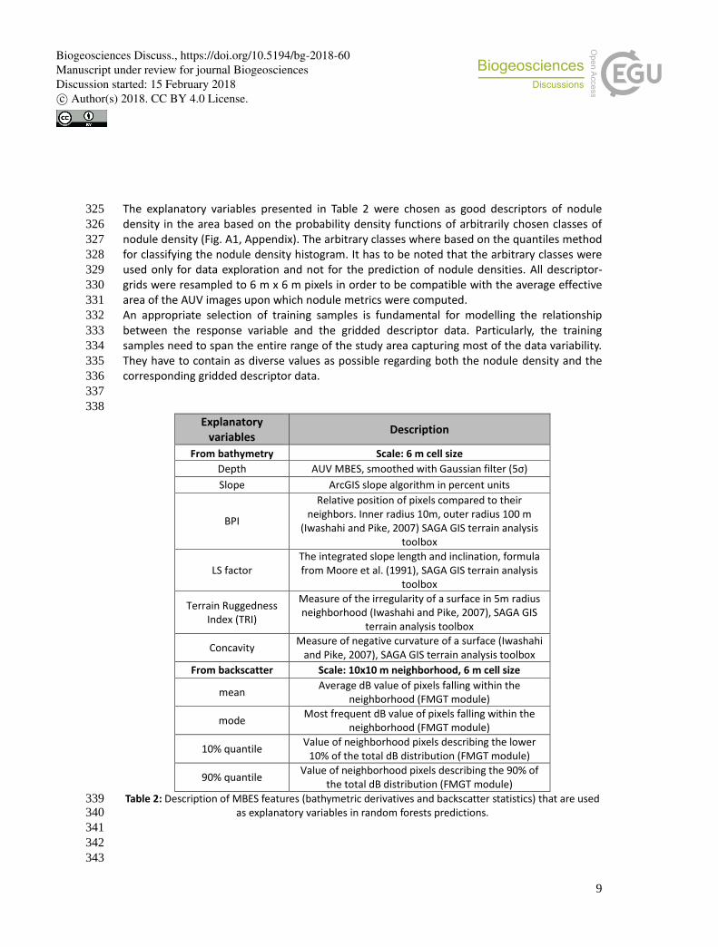
Acoustic

class

PORT: (38o & 40o) central

value (dB)

STARBOARD: (40o & 42o)

central value (dB)

1 -60.7 -61.2

2 -59.4 -59.7

3 -57.4 -58.1

4 -56.3 -56.3

5 -54.8 -54.8

6 -52.8 -52.7

Table 3: Averaged central dB values of the Gaussians derived from reference beam angles on both sides 372 of the AUV MBES. 373

374


11

3.3 ISODATA applied to BS data 375

376

The ISODATA algorithm was applied to the mean, mode, 10% and 90% quantiles of the 377

backscatter mosaic. These datasets are considered more suitable than the raw backscatter 378

data, as they hold a more realistic representation of backscatter spatial variability and they are 379

slightly correlated (correlation coefficients: 0.5-0.9) with the mean backscatter. The ISODATA 380

algorithm was set to produce an optimal number of clusters for different ranges of cluster 381

amounts (minimum number of clusters from 2 to 5; maximum number of clusters from 6 to 382

10). The results for all possible pairs regarding the minimum and maximum clusters were 383

divided, indicating five or six clusters as optimal. To have comparable results with the Bayesian 384

method, six clusters were selected for further analyses. Although the algorithm does not 385

output classes with ordering, the ISODATA classes were reclassified based on their nodule 386

statistics to be comparable with Bayesian results (see discussion section). The classes show a 387

decreasing amount of nodules from north to south with the nodule-free areas being 388

sufficiently demarcated (Fig. 4B). 389

390

391

392

3.4 Random Forest predictions using bathymetry derivatives and BS data 393

394

The RF was performed in two steps: the training and the prediction step. First a sensitivity test 395

was carried out using different percentages of training samples (Fig. 5B) and fitting models 396

with 200 and 1000 trees. This test is essential for examining the optimal settings prior to 397

applying a predictive model. It also helps in quantifying the stability of results (given the 398

random character of the process) by running the model with optimal settings repeatedly. For 399

quantifying the model accuracy we used the percentage of variance explained by the out-of-400

bag samples (RF algorithm output report) whereas for assessing the prediction results, 401

calculation of R2 was applied for measuring the correlation between the predicted and 402

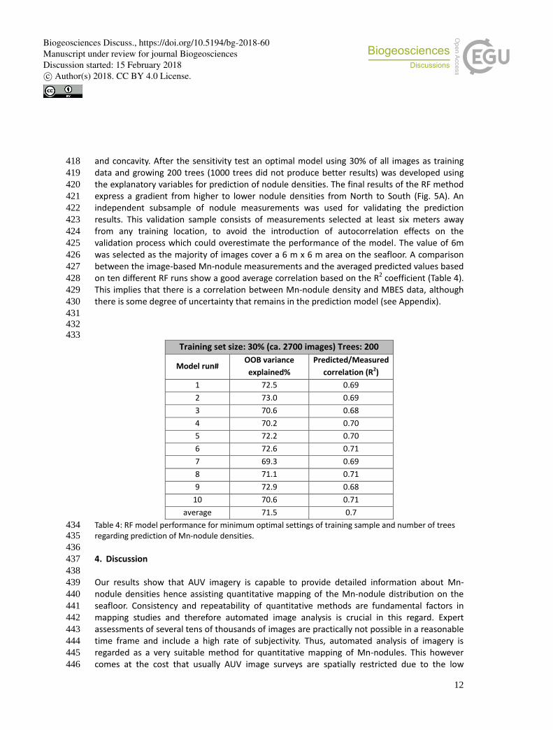
measured nodule density. According to the sensitivity analysis, a training set with 30% of the 403

total amount of images with Mn-nodule statistics was sufficient to explain more than 70% of 404

the variance of the out-of-bag sub-sample when training 200 trees. It was also found that this 405

accuracy value is not improving significantly when increasing the training sample size (Fig. 5B). 406

By maintaining the same amount of training samples (30% of the total images acquired, ca. 407

2700 images) while using ten different parts of the data as training sample (ten-fold cross-408

validation), the model performance was relatively consistent (69-72%) regarding the out-of-409

bag variance explained (Table 4). These results refer to the Mn-nodules m-2 analyses. In 410

addition we tested the predictability of the 2D size of nodules using the 50% and 75% 411

quantiles of 2D sizes in square centimetres. The resulting out-of-bag variance explained was 412

found to be much lower (35-40%), independently from the number of trees and the size of the 413

training sample set. By using the results from the ten-fold cross-validation (or sensitivity test) 414

we extracted the mean importance score of each bathymetry and backscatter parameter (Fig 415

6C). Considering the prediction of Mn-nodules m-2, the mean backscatter data was found to be 416

the most influencing variable which constantly scored first, followed by the BPI, bathymetry 417


12

and concavity. After the sensitivity test an optimal model using 30% of all images as training 418

data and growing 200 trees (1000 trees did not produce better results) was developed using 419

the explanatory variables for prediction of nodule densities. The final results of the RF method 420

express a gradient from higher to lower nodule densities from North to South (Fig. 5A). An 421

independent subsample of nodule measurements was used for validating the prediction 422

results. This validation sample consists of measurements selected at least six meters away 423

from any training location, to avoid the introduction of autocorrelation effects on the 424

validation process which could overestimate the performance of the model. The value of 6m 425

was selected as the majority of images cover a 6 m x 6 m area on the seafloor. A comparison 426

between the image-based Mn-nodule measurements and the averaged predicted values based 427

on ten different RF runs show a good average correlation based on the R2 coefficient (Table 4). 428

This implies that there is a correlation between Mn-nodule density and MBES data, although 429

there is some degree of uncertainty that remains in the prediction model (see Appendix). 430

431 432 433

Training set size: 30% (ca. 2700 images) Trees: 200

Model run# OOB variance

explained%

Predicted/Measured

correlation (R2)

1 72.5 0.69

2 73.0 0.69

3 70.6 0.68

4 70.2 0.70

5 72.2 0.70

6 72.6 0.71

7 69.3 0.69

8 71.1 0.71

9 72.9 0.68

10 70.6 0.71

average 71.5 0.7

Table 4: RF model performance for minimum optimal settings of training sample and number of trees 434 regarding prediction of Mn-nodule densities. 435

436

4. Discussion 437

438

Our results show that AUV imagery is capable to provide detailed information about Mn-439

nodule densities hence assisting quantitative mapping of the Mn-nodule distribution on the 440

seafloor. Consistency and repeatability of quantitative methods are fundamental factors in 441

mapping studies and therefore automated image analysis is crucial in this regard. Expert 442

assessments of several tens of thousands of images are practically not possible in a reasonable 443

time frame and include a high rate of subjectivity. Thus, automated analysis of imagery is 444

regarded as a very suitable method for quantitative mapping of Mn-nodules. This however 445

comes at the cost that usually AUV image surveys are spatially restricted due to the low 446


13

altitude above the seafloor. For larger scale quantitative mapping of nodule fields, AUV 447

imagery data need to get spatially linked with AUV hydro-acoustic data supporting with data 448

from all regions of interest at the seafloor. Results from image analysis can then be used as 449

alternative information for acoustic class validation and predictive mapping. Although image 450

analysis results do not constitute ground-truth information they are the best available data to 451

correlate with acoustic classification and prediction results. By exploring the relationship 452

between Mn-nodule data with bathymetry, bathymetric derivatives and acoustic backscatter, 453

we aim to identify potential linkages that allow extrapolation of nodule information to larger 454

areas to assess mineral resources, determine benthic habitats or learn about geological 455

processes that might influence nodule growth. The following paragraphs discuss the 456

performance of the applied classification and prediction methods highlighting the potential 457

use of high resolution Mn-nodule density maps by considering various sources of errors 458

induced throughout the data analyses. 459

460

461

4.1 Fine scale spatial variability of Mn-nodule density 462

463

Both, the unsupervised classifications (ISODATA, Bayesian) and the random forest prediction 464

results are largely comparable to the nodule detection measurements map (Fig. 6). Hence, 465

both classification and prediction data, and nodule measurements reflect a similar spatial 466

distribution pattern of nodule densities. The Mn-nodule densities seen in the imagery highlight 467

a pattern of alternating high and low density bands on bathymetric slope features. According 468

to studies on the fine scale (tens of meters) distribution of Mn-nodules as summarized by 469

Margolis and Burns (1976) higher nodule densities are related to hilltops, slopes and the foot 470

of slopes. The authors particularly highlighted that e.g. nodule sizes vary significantly over 471

short distances; unfortunately there were no methods to capture this variability sufficiently at 472

the time of this study. The correlation to the bathymetry is supported by the variable 473

importance plot of the RF model (Fig. 5C). This plot shows that both bathymetry and 474

backscatter features contribute significantly to the prediction of the Mn-nodule densities with 475

variables such as mean backscatter intensity, fine scale BPI, and concavity as good predictors. 476

The predictive potential of these variables needs to be validated in future studies using MBES 477

data from different study areas. 478

479

Both unsupervised acoustic classes and the Random Forest prediction suggest a gradient of 480

decreasing nodule densities from north to south while the RF quantitative map (Fig. 5A) shows 481

more gradual changes regarding the fine-scale spatial distribution of Mn-nodules. The 482

northern part of the MBES survey is located very close to, and partly within, a seamount area. 483

According to towed camera video footage these seamounts comprise ancient volcanoes that 484

are now covered with deep sea fine sediments. In addition, a few pillow-basalt outcrops were 485

found along with basalt slabs being exposed on the seamount slopes. Greater nodule densities 486

can be observed from these images suggesting that accumulated nodules or exposed basalt 487

rocks may be assigned to the same acoustic class that represents higher acoustic intensities. In 488

the random forest prediction, high nodule densities could be confused with basalt rock as well 489


14

(Fig. 5A, black arrows). Video data can be used in order to differentiate these seafloor types in 490

the acoustic classes. Greater nodule densities in the vicinity of the seamounts area can be 491

explained by the findings presented by Vineesh et al. (2009) and Sharma et al., (2013). These 492

two studies propose that in the proximity of abyssal hills and slopes, abundant basalt 493

fragments act as nodule nuclei that favour nodule development. Away from the seamount 494

area, the nodule density variations follow a banded pattern of high and low density 495

alternations with localized depressions representing nodule-free areas (Fig. 2B). The band-496

pattern variation is not fully understood by the datasets available in this study; however, it is 497

assumed that it is the result of a combination of the deep sea benthic boundary layer 498

hydrodynamics, local sediment movement and active tectonics that impacts pore fluid 499

migration. It is not clear why and how the nodule-free areas are formed and why we observe 500

moderate nodule densities in broad deep plains of the area. Margolis and Burns (1977) suggest 501

that bathymetric valleys are more influenced by sedimentation hence not favouring nodule 502

growth, but that hill tops and bathymetric slopes are covered by a greater amount of nodules 503

due to a lower impact of local sedimentation. Whether this explanation is also true for the 504

described study area remains speculative. In any case, backscatter data clearly indicate where 505

areas of higher and lower Mn-nodule densities exist, allowing for future investigations of the 506

underlying factors. 507

508

509

510

4.2 Assessing the Mn-nodule acoustic classification 511

512

To assess the performance of unsupervised classification methods in clustering homogeneous 513

areas of Mn-nodules, we examined the within- and between-class variability of the Mn-514

nodules densities (nodules m-2). The assessment is based on the descriptive statistics of nodule 515

measurements from each class (Table 5) and box-plots of nodules m-2 from each class (Fig. 7). 516

The box-plots assist to better illustrate the separation between classes as well. 517

To evaluate the separation of Mn-nodule densities that fall within different acoustic classes 518

(Bayesian and ISODATA), we performed a Welch ANOVA along with a Games-Howell test for 519

testing whether the mean values between the classes differ significantly. This test was 520

selected, because the Levene’s test (Martin & Bridgmon, 2012) indicated that there is no 521

homogeneity between the class variances for both classification methods (p<<0.05). 522

Particularly the results of the Welch ANOVA for nodule populations belonging to the same 523

Bayesian class (F(5,905)=700, p=<<0.05) and ISODATA (F(5, 2520)=810, p<<0.05) support the 524

finding that the mean values of Mn-nodules densities differ significantly between the different 525

classes. This finding supports that classification results effectively resolve acoustically 526

homogenous areas of nodule patches which are statistically distinct to each other. 527

Regarding the Bayesian classification results, the ordinal type of the classes can be noticed 528

both in the statistics and the box-plots (Table 5, Fig. 7A). The mean and median values of 529

nodules m-2 are increasing with increasing class number suggesting that higher backscatter 530

values are related to higher nodule densities. Class 1 represents the lowest nodule densities 531

but without including samples of zero nodules, this would make this class more distinguishable 532

with an even lower mean value. Some class overlap can be observed in the box-plot for the 533


15

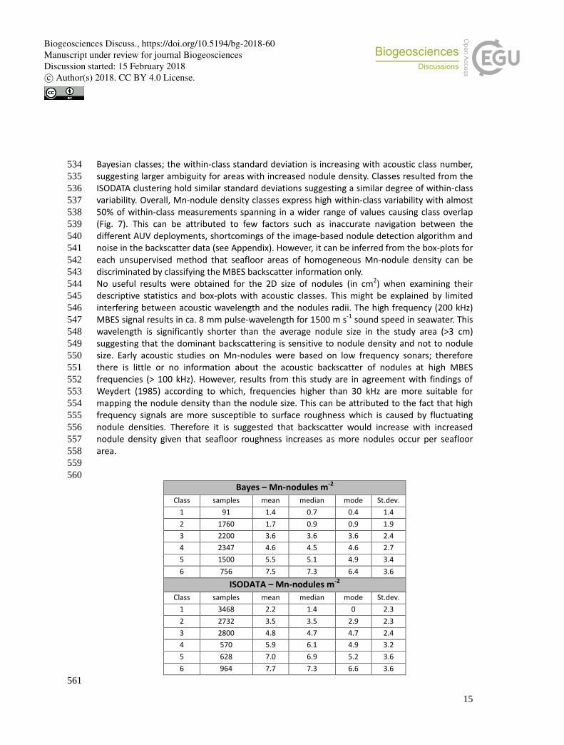
Bayesian classes; the within-class standard deviation is increasing with acoustic class number, 534

suggesting larger ambiguity for areas with increased nodule density. Classes resulted from the 535

ISODATA clustering hold similar standard deviations suggesting a similar degree of within-class 536

variability. Overall, Mn-nodule density classes express high within-class variability with almost 537

50% of within-class measurements spanning in a wider range of values causing class overlap 538

(Fig. 7). This can be attributed to few factors such as inaccurate navigation between the 539

different AUV deployments, shortcomings of the image-based nodule detection algorithm and 540

noise in the backscatter data (see Appendix). However, it can be inferred from the box-plots for 541

each unsupervised method that seafloor areas of homogeneous Mn-nodule density can be 542

discriminated by classifying the MBES backscatter information only. 543

No useful results were obtained for the 2D size of nodules (in cm2) when examining their 544

descriptive statistics and box-plots with acoustic classes. This might be explained by limited 545

interfering between acoustic wavelength and the nodules radii. The high frequency (200 kHz) 546

MBES signal results in ca. 8 mm pulse-wavelength for 1500 m s-1 sound speed in seawater. This 547

wavelength is significantly shorter than the average nodule size in the study area (>3 cm) 548

suggesting that the dominant backscattering is sensitive to nodule density and not to nodule 549

size. Early acoustic studies on Mn-nodules were based on low frequency sonars; therefore 550

there is little or no information about the acoustic backscatter of nodules at high MBES 551

frequencies (> 100 kHz). However, results from this study are in agreement with findings of 552

Weydert (1985) according to which, frequencies higher than 30 kHz are more suitable for 553

mapping the nodule density than the nodule size. This can be attributed to the fact that high 554

frequency signals are more susceptible to surface roughness which is caused by fluctuating 555

nodule densities. Therefore it is suggested that backscatter would increase with increased 556

nodule density given that seafloor roughness increases as more nodules occur per seafloor 557

area. 558

559

560

Bayes – Mn-nodules m-2

Class samples mean median mode St.dev.

1 91 1.4 0.7 0.4 1.4

2 1760 1.7 0.9 0.9 1.9

3 2200 3.6 3.6 3.6 2.4

4 2347 4.6 4.5 4.6 2.7

5 1500 5.5 5.1 4.9 3.4

6 756 7.5 7.3 6.4 3.6

ISODATA – Mn-nodules m-2

Class samples mean median mode St.dev.

1 3468 2.2 1.4 0 2.3

2 2732 3.5 3.5 2.9 2.3

3 2800 4.8 4.7 4.7 2.4

4 570 5.9 6.1 4.9 3.2

5 628 7.0 6.9 5.2 3.6

6 964 7.7 7.3 6.6 3.6

561


16

Table 5: Descriptive statistics highlighting the within-class variability of Mn-nodules for both 562 classification methods. 563

564

565

566

4.3 Implications of acoustic mapping on Mn-nodule resource assessment and benthic habitat 567

characterization 568

569

Obtaining high resolution seafloor acoustic classes and quantitative spatial predictions of the 570

Mn-nodule density provides useful information for deep sea mining and impact management. 571

The obvious application is a more realistic resource assessment (total tonnage of Mn-nodules 572

per area) which can assist a better delineation of particular areas with mining interest on large 573

and small scales. Resource assessment can be based on semi-quantitative information 574

provided by acoustic classes that correspond to particular Mn-nodule densities or quantitative 575

results from the RF predictive map. 576

577

In addition, quantitative maps of Mn-nodule densities can be used to support extrapolations of 578

benthic biota densities to seafloor areas where benthic information is not available. This is 579

possible by considering the nodule substrate as surrogate for habitat mapping of certain biota. 580

Surrogacy for mapping deep sea ecosystems has been incorporated in the study of Anderson 581

et al. (2011); the authors point out, that geomorphic classes can be used for discriminating 582

habitats in broad scales of tens to hundreds of kilometres. They also highlight that any 583

surrogacy approach should be based on the correlation between the physical variables (e.g. 584

bathymetry, backscatter) and the biological patterns that appear in the study area. In 585

Vanreussel et al. (2016) and Amon et al. (2016) it is shown that seafloor covered with more 586

Mn-nodules features higher epifaunal densities. This relation might be further evaluated to 587

have a better and verified relationship between nodule and biota densities allowing estimating 588

biota abundances in larger areas that have only been mapped acoustically. 589

590

591

5. Conclusions 592

593

AUV-based optical and acoustic mapping at high spatial resolution opens up new opportunities 594

for mapping Mn-nodule fields. In this study, automated image analysis provided dense, 595

quantitative information about Mn-nodules at fine scale. This information offers useful insights 596

about the fine scale variability of Mn-nodule densities while it can be utilized for correlations 597

with seafloor acoustic classes and predictive mapping. It was found that the Mn-nodule 598

density within a 500 m x 500 m photo mosaic varies in a pattern of alternating bands (with 599

denser and sparser amounts of nodules) according with smooth bathymetric slopes with a 600

preference of increased nodule occurrence at concave seafloor morphologies. Areas with 601

different nodule densities produced distinct backscatter classes that distinguished nodule 602

populations with distinct mean density values. This suggests that Mn-nodule densities can be 603

efficiently mapped with high resolution hydro-acoustic data. In addition, applying machine 604

learning methodology showed great potential in quantitative predictive mapping of Mn-605


17

nodules through modelling the complex relation between image-derived nodule metrics with 606

bathymetric derivatives and backscatter statistics. In essence, by using a relatively small 607

amount of AUV images (ca. 2700) as the training set it was possible to obtain a 70% correlation 608

between predicted and measured Mn-nodule densities. High quality and spatial resolution 609

AUV hydro-acoustic and optical data can provide a fast and less costly mean for Mn-nodule 610

mapping. This has three major implications in deep sea studies: 1) it raises questions about 611

what causes the Mn-nodules to follow the fine scale bathymetric morphology, 2) it assists in 612

better resource assessment of Mn-nodules and provides the information needed for planning 613

the optimal mining path and 3) it provides more accurate information about Mn-nodule 614

substrate as a benthic habitat, hence it can be utilized for better understanding the deep sea 615

ecology and ecological impact of potential Mn-nodule mining. 616

617

618

Acknowledgements 619

This study was based on data acquired during cruise SO242-1 which is part of the JPIO 620

initiative. We thank Marcel Rothenbeck and Anja Steinführer for pre-processing of the AUV 621

MBES data and providing them in various formats. In addition we thank Anne Peukert and Dr. 622

Inken Preuss for their useful comments in proof-reading the manuscript. This is publication ## 623

of the Deep Sea monitoring Group at GEOMAR. 624

625

626

627

References 628

629

630 Agterberg, F. P., and Bonham‐Carter, G.F.: ,Logistic regression and weights of evidence modeling in 631

mineral exploration, Proc. 28th Interna. Symp. Computer Applications in the Mineral Industries, 632

Golden, Colorado, 483‐490,1999. 633

Alevizos, E., Snellen, M., Simons, D.G., Siemes, K., and Greinert, J.,: Acoustic discrimination of relatively 634

homogeneous fine sediments using Bayesian classification on MBES data. Mar Geol, 370, 31–42. 635

doi:10.1016/j.margeo.2015.10.007, ISSN 0025-3227, 2015. 636

Amiri-Simkooei, A.R., Snellen, and M., Simons, D.G.,: River bed sediment classification using MBES 637

backscatter data, Journal of the Acoustic Society of America,126, 1724–1738,2009. 638

Amon, D. J., Ziegler, A. F., Dahlgren, T. G., Glover, A. G., Goineau, A., Gooday, A. J., Wiklund, H.,and 639

Smith, C. R.: First insights into the abundance and diversity of abyssal megafauna in a 640

polymetallic-nodule region in the eastern Clarion-Clipperton Zone,Sci Rep 6:30492. 641

doi:10.1038/srep30492, 2016 642

Anderson, T.J., Nichol, S.L., Syms, C., Przeslawski, and Harris, P.T.,: Deep-sea bio-physical variables as 643

surrogates for biological assemblages, an example from the Lord Howe Rise, Deep Sea Research 644

Part II: Topical Studies in Oceanography, 58, 979-991,2011. 645


18

Blondel, P. and Gomez Sichi,O.,: Textural analyses of multibeam sonar imagery from Stanton Banks, 646

Northern Ireland continental shelf. Applied Acoustics, 70, 1288–1297,2009. 647

Bluhm, H. : Monitoring megabenthic communities in abyssal manganese nodule sites of the East 648

Pacific Ocean in association with commercial deep-sea mining. Aquatic Conservation, Marine 649

and Freshwater Ecosystems 4, 187–201, 1994 650

Breiman, L.,: RandomForests.Mach.Learn.45,5–32, 2001. 651

Carranza, E. J. M., and Hale, M.,: Geologically constrained fuzzy mapping of gold mineralization 652

potential, Baguio district, Philippines, Natural Resources Research 10, 125‐136, 2001. 653

Chakraborty, B., Pathak, D., Sudhakar, M. and Raju, Y. S.: Determination of Nodule Coverage Parameters 654

Using Multibeam Normal Incidence Echo Characteristics: A Study in the Indian Ocean, Marine 655

Georesources and Geotechnology, 15, 33–48.,doi: 10.1080/10641199709379933,1996. 656

Che Hasan, R., Ierodiaconou, D., Laurenson, L., and Schimel, A.,: Integrating multibeam backscatter 657

angular response, mosaic and bathymetry data for benthic habitat mapping. PLoS ONE, 658

doi:10.1371/journal.pone.0097339,2014. 659

de Moustier, C.: Inference of manganese nodule coverage from Seabeam acoustic backscattering data. 660

Geophysics, 50, 989–1005,1985. 661

Díaz, J. V. M.,: Analysis of Multibeam Sonar Data for the Characterization of Seafloor Habitats, MEng 662

Thesis, University of New Brunswick, pp. 153,1999. 663

Dunn, J. C.,: A Fuzzy Relative of the ISODATA Process and Its Use in Detecting Compact Well-Separated 664

Clusters”. Journal of Cybernetics., 3, 32-57, 1973. 665

Gislason, P.O., Benediktsson, J.A., and Sveinsson J.R.,: Random Forests for land cover classification, 666

Pattern Recognition Letters, Volume 27, Issue 4, 294-300, ISSN 0167-8655, 667

http://dx.doi.org/10.1016/j.patrec.2005.08.011, 2006. 668

Hühnerbach, V., Blondel, Ph., Huvenne, V., and Freiwald, A.,: Habitat mapping on a deepwater coral reef 669

off Norway, with a comparison of visual and computerassisted sonar imagery interpretation. In: 670

Todd B, Greene G, editors. Habitat mapping. Geological association of Canada special paper, vol. 671

47. 297–308, 2008. 672

ISA (2010). A Geological Model of Polymetallic Nodule Deposits in the Clarion-Clipperton Fracture 673

Zone. Technical Study: No. 6, International Seabed Authority, Kingston, Jamaica. 674

http://www.isa.org.jm/files/documents/EN/Pubs/GeoMod-web.pdf 675

Iwahashi, J., and Pike, R.J.,: Automated classifications of topography from DEMs by an unsupervised 676

nested-means algorithm and a three-part geometric signature. Geomorphology, 86, 409–440, 677

2007. 678

Ko, Y., Lee, S., Kim, J., Kim, K.,H., and Jung, M.,S.,: Relationship between Mn nodule abundance and 679

other geological factors in the northeastern Pacific: application of GIS and probability method, 680

Ocean Sci. J. 41(3),149-161,2006. 681

Kwasnitschka, T., Köser, K., Sticklus, J., Rothenbeck, M., Weiß, T., Wenzlaff, E., Schoening, T., Triebe, 682

L., Steinführer, A., Devey, C., and Greinert, J., : DeepSurveyCam—A Deep Ocean Optical 683

Mapping System, Sensors 16 (2),164,2016 684

Lee, S.,H., and Kim, K.H.,: Side-scan sonar characteristics and manganese nodule abundance in the 685

Clarion-Clipperton Fracture Zones NE equatorial Pacific, Mar. Georesour. Geotech, 22, 103-114, 686

2004. 687


19

Lucieer, V., Hill, N.A., Barrett, N.S., and Nichol S.: Do marine substrates ‘look’ and ‘sound’ the same? 688

Supervised classification of multibeam acoustic data using autonomous underwater vehicle 689

images. Estuarine Coastal Shelf Sci.117, 94–106,,2013. 690

Margolis, S. V., and Burns, R. G.,: Pacific deep‐sea manganese nodules: their distribution, composition 691

and origin. Annual Review of Earth and Planetary Sciences, 4, 229-263,1976. 692

Martin, W. E., and Bridgmon, K. D.,: Quantitative and statistical research methods: from hypothesis to 693

results. New Jersey: John Wiley & Sons, ISBN: 978-0-470-63182-9,2012. 694

Masson,D. G., and Scanlon, K. M.: Fe-Mn Nodule Field Indicated GIoria, North of the Puerto Rico 695

Trench, Geo-Marine Letters, 208-213,1992. 696

Memarsadeghi, N., Mount, D.M., Netanyahu, N.S., and Moigne, J.L.: A fast implementation of the 697

isodata clustering algorithm. International Journal of Computational Geometry and Applications 698

17, 71–103, 2007. 699

Moore, I.D., Grayson, R.B., and Ladson, A.R.,: Digital terrain modelling: a review of hydrological, 700

geomorphological, and biological applications. Hydrological Processes, 5, 3 – 30, 1991. 701

Okazaki, M., and Tsune, A.,.: Exploration of Polymetallic Nodules Using AUV in the Central Equatorial 702

Pacific, Proc. of the ISOPE Ocean Mining Symposium, Szczecin, Poland, 22-26 September 2013, 703

32-38,2013. 704

Petersen, S., Krätschell, A., Augustin, N., Jamieson, J., Hein, J. R. and Hannington, M. D.: News from the 705

seabed – Geological characteristics and resource potential of deep-sea mineral resources, 706

Marine Policy, 70 , pp. 175-187. DOI 10.1016/j.marpol.2016.03.012, 2016 707

Purser, A., Marcon, Y., Hoving, H.J.T., Vecchione, M., Piatkowski, U., Eason, D., Bluhm, H., and Boetius, 708

A.,: Association of deep-sea incirrate octopods with manganese crusts and nodule fields in the 709

Pacific Ocean, Current Biology, 26, Issue 24, 2016, R1268-R1269, ISSN 0960-9822, 710

http://dx.doi.org/10.1016/j.cub.2016.10.052,2016 711

Roberts, J.J., Best, B.D., Dunn, D.C., Treml, E.A., and Halpin, P.N.,: Marine Geospatial Ecology Tools: An 712

integrated framework for ecological geoprocessing with ArcGIS, Python, R, MATLAB, and C++. 713

Environmental Modelling & Software, 25, 1197-1207. doi: 10.1016/j.envsoft.2010.03.029, 2010. 714

Schoening, T., Kuhn, T., and Nattkemper, T.W.,: Estimation of poly-metallic nodule coverage in benthic 715

images, Proc. of the 41st Conference of the Underwater Mining Institute (UMI),2012. 716

Sharma, R., Khadge, N.H., and Sankar, S.J.,: Assessing the distribution and abundance of seabed 717

minerals from seafloor photographic data in the Central Indian Ocean Basin, International journal 718

of remote sensing, 34 (5), 1691-1706,2013. 719

Simons, D.G., and Snellen, M.,: A Bayesian technique to seafloor classification using multi-beam echo-720

sounder backscatter data. Applied Acoustics, 70, 1258-721

1268,http://dx.doi.org/10.1016/j.apacoust.2008.07.013, 2009. 722

Stephens, D., and Diesing, M.,: A Comparison of Supervised Classification Methods for the Prediction 723

of Substrate Type Using Multibeam Acoustic and Legacy Grain-Size Data. PLoS ONE, 724

doi:10.1371/journal.pone.0093950, 2014. 725

Thiel, H.,: Evaluation of the environmental consequences of polymetallic nodule mining based on the 726

results of the TUSCH Research Association, Deep Sea Research Part II: Topical Studies in 727

Oceanography, 48, (17–18),3433-3452. doi: http://dx.doi.org/10.1016/S0967-0645(01)00051-0, 728

2001 729


20

Vanreusel, A., Hilario, A., Ribeiro, P. A., Menot, L., and Arbizu, P. M.: Threatened by mining, polymetallic 730

nodules are required to preserve abyssal epifauna. Sci. Rep. 6:26808. doi: 731

10.1038/srep26808,2016 732

Vineesh, T. C., Nath, B. N., Banerjee, R., Jaisankar, S. and Lekshmi, V. : Manganese Nodule Morphology 733

as Indicators for Oceanic Processes in the Central Indian Basin, International Geology Review, 51, 734

27–44,2009. 735

Weydert, M.,: Measurements of the acoustic backscatter of selected areas of the deep seafloor and 736

some implications for the assessment of manganese nodule resources, J Acoustical Society of 737

America, 88, 350–366,1990. 738

Weydert, M.,: Measurement of acoustic backscattering of the deep seafloor using a deeply towed 739

vehicle. A technique to investigate the physical and geological properties of the deep seafloor 740

and to assess manganese nodule resources, Ph.D thesis, San Diego: University of California, 1985. 741

742

743

744

745

746


21

Fig. 1: A) The DISCOL area location in the Peru Basin (red star). B) Ship-based, shaded bathymetry of the wider DISCOL area with 40 m pixel size. The black rectangle represents the boundaries of the AUV MBES dataset used in this study (Fig.2).

747

748


22

749

Fig. 2: A) AUV MBES bathymetry with black lines indicating the tracks of the AUV image survey. Closely spaced track lines covering a rectangular area in the lower part of the image correspond to the areas

shown in Figures 3A & 6A-D. B) AUV backscatter mosaic. The polygons delineated in red represent nodule-free areas as observed from underwater video data.

750

751

752

753

754


23

Fig. 3: A) Points with nodule measurements derived from automated nodule detection, draped

on AUV bathymetry, showing Mn-nodules per square meter from perspective view, B) Longitudinal section of bathymetric profile from same area highlighting the local scale morpho-bathymetry of Mn-

nodule fields. 755

756

757


24

Fig. 4: A) Bayesian classification map based on AUV backscatter beam data, B) ISODATA classification map based on AUV backscatter neighbourhood statistics (mean, mode, 10th Q and 90th Q, see Table 2). 758

759

760

761

762


25

Fig. 5: A) Random forests prediction map of Mn-nodules densities, Sensitivity analysis results: B)

Percentage of training sample size and performance of RF model in terms of percentage of variance explained (out-of-bag). C) Importance scores of MBES explanatory variables, based on average

percentage increase of mean prediction error from ten model runs.

763

764

765

766

767

768

769

770

771

772

773


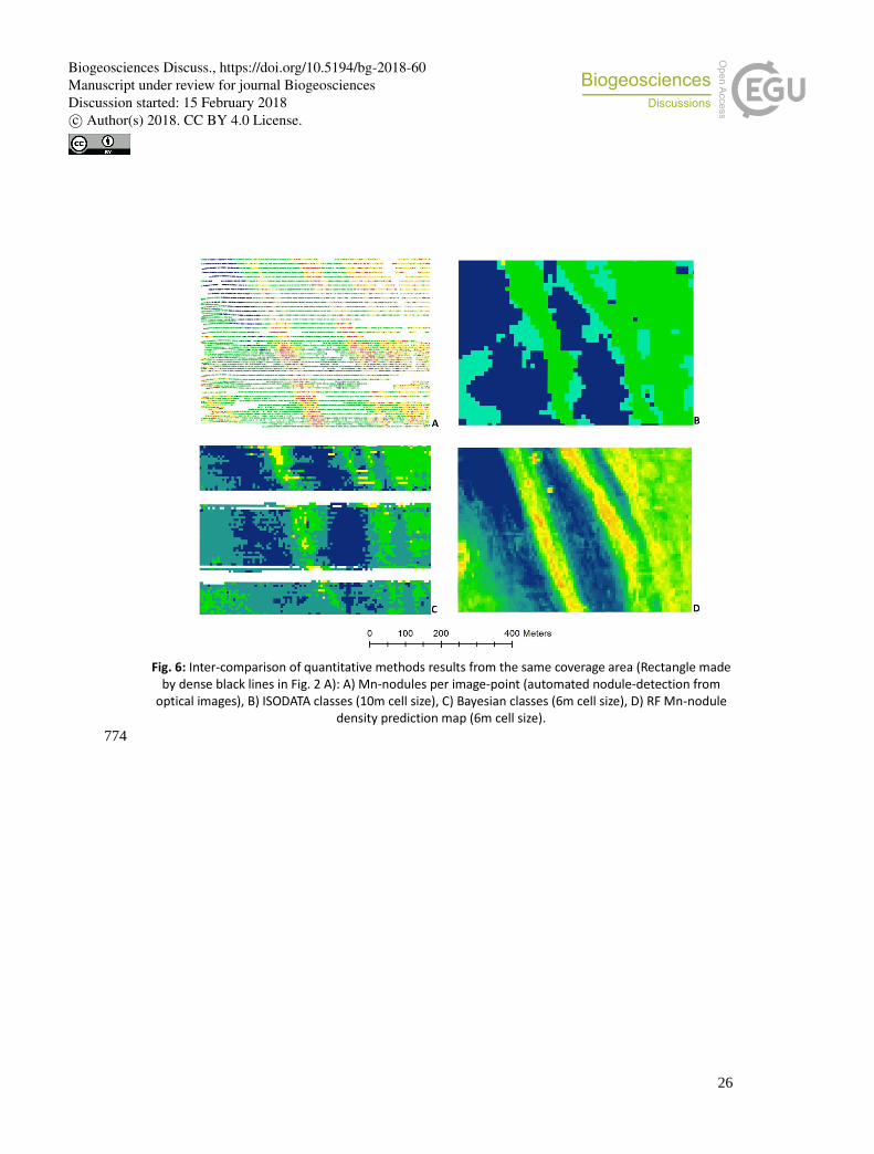
26

Fig. 6: Inter-comparison of quantitative methods results from the same coverage area (Rectangle made

by dense black lines in Fig. 2 A): A) Mn-nodules per image-point (automated nodule-detection from optical images), B) ISODATA classes (10m cell size), C) Bayesian classes (6m cell size), D) RF Mn-nodule

density prediction map (6m cell size).

774


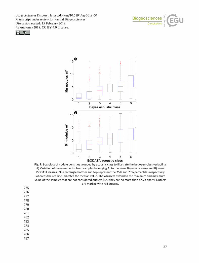
27

Fig. 7: Box-plots of nodule densities grouped by acoustic class to illustrate the between-class variability.

A) Variation of measurements, from samples belonging A) to the same Bayesian classes and B) same ISODATA classes. Blue rectangle bottom and top represent the 25% and 75% percentiles respectively whereas the red line indicates the median value. The whiskers extend to the minimum and maximum

value of the samples that are not considered outliers (i.e.: they are no more than ±2.7σ apart). Outliers are marked with red crosses.

775

776

777

778

779

780

781

782

783

784

785

786

787


28

APPENDIX 788

789

Fig. A1: Data exploration results showing probability density functions for arbitrary classes of nodules per image (<10: no nodules, 10-184: low, 185-270: mid, >270: high) for A) bathymetry and derivatives

and B) Backscatter and neighbourhood statistics.


29

APPENDIX A1 790

Error sources in quantitative Mn-nodule mapping 791

A few error sources need to be considered when performing seafloor classification and nodule 792

density estimates with optical and acoustic data acquired during multiple AUV deployments. 793

794

1) Noisy backscatter data: Since the Bayesian approach uses the raw backscatter data, 795

any final classification is susceptible to the effects of noise. Hence, beam incidence 796

angles less than 20 degrees were discarded due to extreme nadir noise effects. The 797

ISODATA classification was based on the backscatter mosaic and its statistics which 798

are also affected mainly by nadir specular noise. It is thus strongly recommended 799

that backscatter data are properly corrected for geometric and sensor-related effects 800

during pre-processing and grids are also filtered/smoothed before the final 801

classification. 802

803

2) AUV navigation: As exact underwater navigation in 4 km water depth is generally a 804

difficult task, relative misalignments of data from different deployments are very 805

common. Differences in absolute positioning between two deployments can easily 806

amount to 100 m. Thus correlating image based nodule densities from one 807

deployment with backscatter values from another dive might introduce correlation 808

errors that also impact predictability. Although the large scale spatial pattern of 809

classes is well defined, these misalignments can slightly alter the position of class 810

boundaries causing disagreement with the nodule density measurements in places. A 811

correct and verified re-navigation of all AUV-tracks is important for all subsequent 812

analyses. This was done during this study, but slight misalignments remain. 813

814

3) Nodule sediment blanketing: The effect of Mn-nodules being blanketed by sediment 815

needs to be considered as a source of error here as the individual nodule size and 816

thus the seafloor coverage might be underestimated by automated annotation. Apart 817

from natural sedimentation, the re-deposition of the plume cloud caused by 818

ploughing during the first disturbance experiment (conducted in 1989), has covered 819

certain parts of the nodule field which might lead to a lower nodule densities in 820

those areas. This effect can artificially reduce the correlation between acoustic 821

classes and Mn-nodule densities given that backscatter is not affected by sediment 822

blanketing. 823

824


Documents

Quantification of th e fine -scale distribution of Mn ... · A strong influence of mean backscatter, fine scale BPI ... 72 1996) , showed that the ... 134 (obtained by