Large Scale Fine-Grained Categorization and Domain-Specific Transfer

Learning

Yin Cui1,2∗ Yang Song3 Chen Sun3 Andrew Howard3 Serge Belongie1,2

1Department of Computer Science, Cornell University 2Cornell Tech 3Google Research

Abstract

Transferring the knowledge learned from large scale

datasets (e.g., ImageNet) via fine-tuning offers an effective

solution for domain-specific fine-grained visual categoriza-

tion (FGVC) tasks (e.g., recognizing bird species or car

make & model). In such scenarios, data annotation often

calls for specialized domain knowledge and thus is difficult

to scale. In this work, we first tackle a problem in large scale

FGVC. Our method won first place in iNaturalist 2017 large

scale species classification challenge. Central to the suc-

cess of our approach is a training scheme that uses higher

image resolution and deals with the long-tailed distribu-

tion of training data. Next, we study transfer learning via

fine-tuning from large scale datasets to small scale, domain-

specific FGVC datasets. We propose a measure to estimate

domain similarity via Earth Mover’s Distance and demon-

strate that transfer learning benefits from pre-training on a

source domain that is similar to the target domain by this

measure. Our proposed transfer learning outperforms Im-

ageNet pre-training and obtains state-of-the-art results on

multiple commonly used FGVC datasets.

1. Introduction

Fine-grained visual categorization (FGVC) aims to dis-

tinguish subordinate visual categories. Examples include

recognizing natural categories such as species of birds [58,

54], dogs [28] and plants [39, 59]; or man-made categories

such as car make & model [32, 63]. A successful FGVC

model should be able to discriminate categories with subtle

differences, which presents formidable challenges for the

model design yet also provides insights to a wide range of

applications such as rich image captioning [3], image gen-

eration [5], and machine teaching [27, 37].

Recent advances on Convolutional Neural Networks

(CNNs) for visual recognition [33, 48, 51, 20] have fu-

eled remarkable progress on FGVC [36, 11, 69]. In gen-

eral, to achieve reasonably good performance with CNNs,

∗Work done during internship at Google Research.

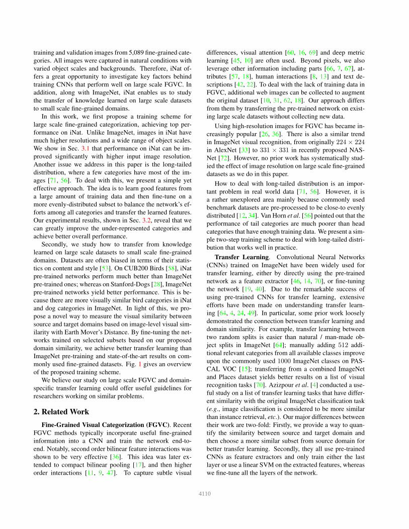
Figure 1. Overview of the proposed transfer learning scheme.

Given the target domain of interest, we pre-train a CNN on the

selected subset from the source domain based on the proposed do-

main similarity measure, and then fine-tune on the target domain.

one needs to train networks with vast amounts of supervised

data. However, collecting a labeled fine-grained dataset of-

ten requires expert-level domain knowledge and therefore

is difficult to scale. As a result, commonly used FGVC

datasets [58, 28, 32] are relatively small, typically contain-

ing around 10k of labeled training images. In such a sce-

nario, fine-tuning the networks that are pre-trained on large

scale datasets such as ImageNet [12] is often adopted.

This common setup poses two questions: 1) What are

the important factors to achieve good performance on large

scale FGVC? Although other large scale generic visual

datasets like ImageNet contain some fine-grained cate-

gories, their images are usually iconic web images that

contain objects in the center with similar scale and simple

backgrounds. With the limited availability of large scale

FGVC datasets, how to design models that perform well

on large scale non-iconic images with fine-grained cate-

gories remains an underdeveloped area. 2) How does one

effectively conduct transfer learning, by first training the

network on a large scale dataset and then fine-tuning it

on domain-specific fine-grained datasets? Modern FGVC

methods overwhelmingly use ImageNet pre-trained net-

works for fine-tuning. Given the fact that the target fine-

grained domain is known, can we do better than ImageNet?

This paper aims to answer the two aforementioned prob-

lems, with the recently introduced iNaturalist 2017 large

scale fine-grained dataset (iNat) [55]. iNat contains 675,170

14109

training and validation images from 5,089 fine-grained cate-

gories. All images were captured in natural conditions with

varied object scales and backgrounds. Therefore, iNat of-

fers a great opportunity to investigate key factors behind

training CNNs that perform well on large scale FGVC. In

addition, along with ImageNet, iNat enables us to study

the transfer of knowledge learned on large scale datasets

to small scale fine-grained domains.

In this work, we first propose a training scheme for

large scale fine-grained categorization, achieving top per-

formance on iNat. Unlike ImageNet, images in iNat have

much higher resolutions and a wide range of object scales.

We show in Sec. 3.1 that performance on iNat can be im-

proved significantly with higher input image resolution.

Another issue we address in this paper is the long-tailed

distribution, where a few categories have most of the im-

ages [71, 56]. To deal with this, we present a simple yet

effective approach. The idea is to learn good features from

a large amount of training data and then fine-tune on a

more evenly-distributed subset to balance the network’s ef-

forts among all categories and transfer the learned features.

Our experimental results, shown in Sec. 3.2, reveal that we

can greatly improve the under-represented categories and

achieve better overall performance.

Secondly, we study how to transfer from knowledge

learned on large scale datasets to small scale fine-grained

domains. Datasets are often biased in terms of their statis-

tics on content and style [53]. On CUB200 Birds [58], iNat

pre-trained networks perform much better than ImageNet

pre-trained ones; whereas on Stanford-Dogs [28], ImageNet

pre-trained networks yield better performance. This is be-

cause there are more visually similar bird categories in iNat

and dog categories in ImageNet. In light of this, we pro-

pose a novel way to measure the visual similarity between

source and target domains based on image-level visual sim-

ilarity with Earth Mover’s Distance. By fine-tuning the net-

works trained on selected subsets based on our proposed

domain similarity, we achieve better transfer learning than

ImageNet pre-training and state-of-the-art results on com-

monly used fine-grained datasets. Fig. 1 gives an overview

of the proposed training scheme.

We believe our study on large scale FGVC and domain-

specific transfer learning could offer useful guidelines for

researchers working on similar problems.

2. Related Work

Fine-Grained Visual Categorization (FGVC). Recent

FGVC methods typically incorporate useful fine-grained

information into a CNN and train the network end-to-

end. Notably, second order bilinear feature interactions was

shown to be very effective [36]. This idea was later ex-

tended to compact bilinear pooling [17], and then higher

order interactions [11, 9, 47]. To capture subtle visual

differences, visual attention [60, 16, 69] and deep metric

learning [45, 10] are often used. Beyond pixels, we also

leverage other information including parts [66, 7, 67], at-

tributes [57, 18], human interactions [8, 13] and text de-

scriptions [42, 22]. To deal with the lack of training data in

FGVC, additional web images can be collected to augment

the original dataset [10, 31, 62, 18]. Our approach differs

from them by transferring the pre-trained network on exist-

ing large scale datasets without collecting new data.

Using high-resolution images for FGVC has became in-

creasingly popular [26, 36]. There is also a similar trend

in ImageNet visual recognition, from originally 224 × 224in AlexNet [33] to 331 × 331 in recently proposed NAS-

Net [72]. However, no prior work has systematically stud-

ied the effect of image resolution on large scale fine-grained

datasets as we do in this paper.

How to deal with long-tailed distribution is an impor-

tant problem in real world data [71, 56]. However, it is

a rather unexplored area mainly because commonly used

benchmark datasets are pre-processed to be close-to evenly

distributed [12, 34]. Van Horn et al. [56] pointed out that the

performance of tail categories are much poorer than head

categories that have enough training data. We present a sim-

ple two-step training scheme to deal with long-tailed distri-

bution that works well in practice.

Transfer Learning. Convolutional Neural Networks

(CNNs) trained on ImageNet have been widely used for

transfer learning, either by directly using the pre-trained

network as a feature extractor [46, 14, 70], or fine-tuning

the network [19, 40]. Due to the remarkable success of

using pre-trained CNNs for transfer learning, extensive

efforts have been made on understanding transfer learn-

ing [64, 4, 24, 49]. In particular, some prior work loosely

demonstrated the connection between transfer learning and

domain similarity. For example, transfer learning between

two random splits is easier than natural / man-made ob-

ject splits in ImageNet [64]; manually adding 512 addi-

tional relevant categories from all available classes improve

upon the commonly used 1000 ImageNet classes on PAS-

CAL VOC [15]; transferring from a combined ImageNet

and Places dataset yields better results on a list of visual

recognition tasks [70]. Azizpour et al. [4] conducted a use-

ful study on a list of transfer learning tasks that have differ-

ent similarity with the original ImageNet classification task

(e.g., image classification is considered to be more similar

than instance retrieval, etc.). Our major differences between

their work are two-fold: Firstly, we provide a way to quan-

tify the similarity between source and target domain and

then choose a more similar subset from source domain for

better transfer learning. Secondly, they all use pre-trained

CNNs as feature extractors and only train either the last

layer or use a linear SVM on the extracted features, whereas

we fine-tune all the layers of the network.

4110

3. Large Scale Fine-Grained Categorization

In this section, we present our training scheme that

achieves top performance on the challenging iNaturalist

2017 dataset, especially focusing on using higher image res-

olution and dealing with long-tailed distribution.

3.1. The Effect of Image Resolution

When training a CNN, for the ease of network design and

training in batches, the input image is usually pre-processed

to be square with a certain size. Each network architecture

usually has a default input size. For example, AlexNet [33]

and VGGNet [48] take the default input size of 224 × 224and this default input size cannot be easily changed be-

cause the fully-connected layer after convolutions requires

a fixed size feature map. More recent networks including

ResNet [20] and Inception [51, 52, 50] are fully convolu-

tional, with a global average pooling layer right after con-

volutions. This design enables the network to take input

images with arbitrary sizes. Images with different resolu-

tion induce feature maps of different down-sampled sizes

within the network.

Input images with higher resolutions usually contain

richer information and subtle details that are important to

visual recognition, especially for FGVC. Therefore, in gen-

eral, higher resolution input image yields better perfor-

mance. For networks optimized on ImageNet, there is a

trend of using input images with higher resolution for mod-

ern networks: from originally 224× 224 in AlexNet [33] to

331 × 331 in recently proposed NASNet [72], as shown in

Table 3. However, most images from ImageNet have a res-

olution of 500 × 375 and contain objects of similar scales,

limiting the benefits we can get from using higher resolu-

tion inputs. We explore the effect of using a wide range

of input image sizes from 299 × 299 to 560 × 560 in iNat

dataset, showing greatly improved performance with higher

resolution inputs.

3.2. Long­Tailed Distribution

The statistics of real world images is long-tailed: a few

categories are highly representative and have most of the

images, whereas most categories are observed rarely with

only a few images [71, 56]. This is in stark contrast to the

even image distribution in popular benchmark datasets such

as ImageNet [12], COCO [34] and CUB200 [58].

With highly imbalanced numbers of images across cat-

egories in iNaturalist dataset [55], we observe poor perfor-

mance on underrepresented tail categories. We argue that

this is mainly caused by two reasons: 1) The lack of training

data. Around 1,500 fine-grained categories in iNat training

set have fewer than 30 images. 2) The extreme class im-

balance encountered during training: the ratio between the

number of images in the largest class and the smallest one is

Input Res. Networks

224× 224 AlexNet [33], VGGNet [48], ResNet [20]

299× 299 Inception [51, 52, 50]

320× 320 ResNetv2 [21], ResNeXt [61], SENet [23]

331× 331 NASNet [72]

Table 1. Default input image resolution for different networks.

There is a trend of using input images with higher resolution for

modern networks.

0 1000 2000 3000 4000 5000Category id sorted by number of images

10 5

10 4

10 3

10 2

Imag

e fre

quen

cy

iNat trainSubset for further fine-tuning

Figure 2. The distribution of image frequency of each category in

the whole training set we used in the first stage training and the

selected subset we used in the second stage fine-tuning.

about 435. Without any re-sampling of the training images

or re-weighting of the loss, categories with more images in

the head will dominate those in the tail. Since there is very

little we can do for the first issue of lack of training data,

we propose a simple and effective way to address the sec-

ond issue of the class imbalance.

The proposed training scheme has two stages. In the first

stage, we train the network as usual on the original imbal-

anced dataset. With large number of training data from all

categories, the network learns good feature representations.

Then, in the second stage, we fine-tune the network on a

subset containing more balanced data with a small learning

rate. The idea is to slowly transfer the learned feature and let

the network re-balance among all categories. Fig. 2 shows

the distribution of image frequency in iNat training set that

we trained on in the first stage and the subset we used in the

second stage, respectively. Experiments in Sec. 5.2 verify

that the proposed strategy yields improved overall perfor-

mance, especially for underrepresented tail categories.

4. Transfer Learning

This section describes transfer learning from the net-

works trained on large scale datasets to small scale fine-

grained datasets. We introduce a way to measure visual sim-

ilarity between two domains and then show how to select a

subset from source domain given the target domain.

4111

4.1. Domain Similarity

Suppose we have a source domain S and a target domain

T . We define the distance between two images s ∈ S and

t ∈ T as the Euclidean distance between their feature rep-

resentations:

d(s, t) = ‖g(s)− g(t)‖ (1)

where g(·) denotes a feature extractor for an image. To bet-

ter capture the image similarity, the feature extractor g(·)needs to be capable of extracting high-level information

from images in a generic, unbiased manner. Therefore, in

our experiments, we use g(·) as the features extracted from

the penultimate layer of a ResNet-101 trained on the large

scale JFT dataset [49].

In general, using more images yields better transfer

learning performance. For the sake of simplicity, in this

study we ignore the effect of domain scale (number of im-

ages). Specifically, we normalize the number of images

in both source and target domain. As studied by Chen et

al. [49], transfer learning performance increases logarith-

mically with the amount of training data. This suggests that

the performance gain in transfer learning resulting from the

use of more training data would be insignificant when we al-

ready have a large enough dataset (e.g., ImageNet). There-

fore, ignoring the domain scale is a reasonable assumption

that simplifies the problem. Our definition of domain simi-

larity can be generalized to take domain scale into account

by adding a scale factor, but we found ignoring the domain

scale already works well in practice.

Under this assumption, transfer learning can be viewed

as moving a set of images from the source domain S to the

target domain T . The work needed to be done by moving

an image to another can be defined as their image distance

in Eqn. 1. Then the distance between two domains can be

defined as the least amount of total work needed. This def-

inition of domain similarity can be calculated by the Earth

Mover’s Distance (EMD) [41, 43].

To make the computations more tractable, we further

make an additional simplification to represent all image fea-

tures in a category by the mean of their features. Formally,

we denote source domain as S = {(si, wsi)}mi=1 and target

domain as T = {(tj , wtj )}nj=1, where si is the i-th cate-

gory in S and wsi is the normalized number of images in

that category; similarly for tj and wtj in T . m and n are

the total number of categories in source domain S and tar-

get domain T , respectively. Since we normalize the number

of images, we have∑m

i=1 wsi =∑n

j=1 wtj = 1. g(si) de-

notes the mean of image features in category i from source

domain, similarly for g(tj) in target domain. Using the de-

fined notations, the distance between S and T is defined as

their Earth Mover’s Distance (EMD):

d(S, T ) = EMD(S, T ) =

∑m,n

i=1,j=1 fi,jdi,j∑m,n

i=1,j=1 fi,j(2)

Northern cardinal (0.3)

Ragdoll (0.2)

Indigo bunting(0.55)

Corgi(0.3)

Boeing 777(0.15)

Tesla Model S(0.5)

0.3

0.2 0.1

0.15

0.25

Feature Space

Figure 3. The proposed domain similarity calculated by Earth

Mover’s Distance (EMD). Categories in source domain and tar-

get domain are represented by red and green circles. The size of

the circle denotes the normalized number of images in that cate-

gory. Blue arrows represent flows from source to target domain by

solving EMD.

where di,j = ‖g(si) − g(tj)‖ and the optimal flow fi,jcorresponds to the least amount of total work by solving the

EMD optimization problem. Finally, the domain similarity

is defined as:

sim(S, T ) = e−γd(S,T ) (3)

where γ is set to 0.01 in all experiments. Fig. 3 illustrates

calculating the proposed domain similarity by EMD.

4.2. Source Domain Selection

With the defined domain similarity in Eqn. 2, we are able

to select a subset from source domain that is more similar

to target domains. We use greedy selection strategy to in-

crementally include the most similar category in the source

domain. That is, for each category si in source domain S ,

we calculate its domain similarity with target domain by

sim({(si, 1)}, T ) as defined in Eqn. 3. Then top k cat-

egories with highest domain similarities will be selected.

Notice that although this greedy way of selection has no

guarantee on the optimality of the selected subset of size k

in terms of domain similarity, we found this simple strategy

works well in practice.

5. Experiments

The proposed training scheme for large scale FGVC is

evaluated on the recently proposed iNaturalist 2017 dataset

(iNat) [55]. We also evaluate the effectiveness of the our

proposed transfer learning by using ImageNet and iNat as

source domains, and 7 fine-grained categorization datasets

as target domains. Sec. 5.1 introduces experiment setup.

Experiment results on iNat and transfer learning are pre-

sented in Sec. 3 and Sec. 5.3, respectively.

4112

5.1. Experiment setup

5.1.1 Datasets

iNaturalist. The iNatrualist 2017 dataset (iNat) [55]

contains 675,170 training and validation images from 5,089

natural fine-grained categories. Those categories belong to

13 super-categories including Plantae (Plant), Insecta (In-

sect), Aves (Bird), Mammalia (Mammal), and so on. The

iNat dataset is highly imbalanced with dramatically differ-

ent number of images per category. For example, the largest

super-category “Plantae (Plant)” has 196,613 images from

2,101 categories; whereas the smallest super-category “Pro-

tozoa” only has 381 images from 4 categories. We combine

the original split of training set and 90% of the validation set

as our training set (iNat train), and use the rest of 10% vali-

dation set as our mini validation set (iNat minival), resulting

in total of 665,473 training and 9,697 validation images.

ImageNet. We use the ILSVRC 2012 [44] splits of

1,281,167 training (ImageNet train) and 50,000 validation

(ImageNet val) images from 1,000 classes.

Fine-Grained Visual Categorization. We evaluate our

transfer learning approach on 7 fine-grained visual cate-

gorization datasets as target domains, which cover a wide

range of FGVC tasks including natural categories like bird

and flower and man-made categories such as aircraft. Table

2 summarizes number of categories, together with number

of images in their original training and validation splits.

5.1.2 Network Architectures

We use 3 types of network architectures: ResNet [20,

21], Inception [51, 52, 50] and SENet [23].

Residual Network (ResNet). Originally introduced by

He et al. [20], networks with residual connections greatly

reduced the optimization difficulties and enabled the train-

ing of much deeper networks. ResNets were later improved

by pre-activation that uses identity mapping as the skip con-

nection between residual modules [21]. We used the latest

version of ResNets [21] with 50, 101 and 152 layers.

Inception. The Inception module was firstly proposed

by Szegedy et al. in GoogleNet [51] that was designed

to be very efficient in terms of parameters and computa-

tions, while achieving state-of-the-art performance. Incep-

tion module was then further optimized by using Batch Nor-

malization [25], factorized convolution [52, 50] and residual

connections [50] as introduced in [20]. We use Inception-

v3 [52], Inception-v4 and Inception-ResNet-v2 [50] as rep-

resentatives for Inception networks in our experiments.

Squeeze-and-Excitation (SE). Recently proposed by

Hu et al. [23], Sequeeze-and-Excitation (SE) modules

achieved the best performance in ILSVRC 2017 [44]. SE

module squeezes responses from a feature map by spatial

average pooling and then learns to re-scale each channel of

FGVC Dataset # class # train # val

Flowers-102 [39] 102 2,040 6,149

CUB200 Birds [58] 200 5,994 5,794

Aircraft [38] 100 6,667 3,333

Stanford Cars [32] 196 8,144 8,041

Stanford Dogs [28] 120 12,000 8,580

NABirds [54] 555 23,929 24,633

Food101 [6] 101 75,750 25,250

Table 2. We use 7 fine-grained visual categorization datasets to

evaluate the proposed transfer learning method.

Inc-v3 299 Inc-v3 448 Inc-v3 560

Top-1 (%) 29.93 26.51 25.37

Top-5 (%) 10.61 9.02 8.56

Table 3. Top-5 error rate on iNat minival using Inception-v3 with

various input sizes. Higher input size yield better performance.

the feature map. Due to its simplicity in design, SE module

can be used in almost any modern networks to boost the per-

formance with little additional overhead. We use Inception-

v3 SE and Inception-ResNet-v2 SE as baselines.

For all network architectures, we follow strictly their

original design but with the last linear classification layer

replaced to match the number of categories in our datasets.

5.1.3 Implementation

We used open-source Tensorflow [2] to implement and

train all the models asynchronously on multiple NVIDIA

Tesla K80 GPUs. During training, the input image was

randomly cropped from the original image and re-sized to

the target input size with scale and aspect ratio augmenta-

tion [51]. We trained all networks using the RMSProp opti-

mizer with momentum of 0.9, and the batch size of 32. The

initial learning rate was set to 0.045, with exponential decay

of 0.94 after every 2 epochs, same as [51]; for fine-tuning

in transfer learning, the initial learning rate is lowered to

0.0045 with the learning rate decay of 0.94 after every 4

epochs. We also used label smoothing as introduced in [52].

During inference, the original image is center cropped and

re-sized to the target input size.

5.2. Large Scale Fine­Grained Visual Recognition

To verify the proposed learning scheme for large scale

fine-grained categorization, we conduct extensive experi-

ments on iNaturalist 2017 dataset. For better performance,

we fine-tune from ImageNet pre-trained networks. If train-

ing from scratch on iNat, the top-5 error rate is ≈ 1% worse.

We train Inception-v3 with 3 different input resolutions

(299, 448 and 560). The effect of image resolution is pre-

sented in Table 3. From the table, we can see that using

higher input resolutions achieve better performance on iNat.

4113

Inc-v3 299 Inc-v3 560 Inc-v4 560 Inc-ResNet-v2 560Network and input image size

0.0

2.0

4.0

6.0

8.0

10.0

Top-

5 er

ror r

ate

(%) 10.61

8.567.02 7.25

9.87

6.605.44 5.63

Before After

Figure 4. Top-5 error rate on iNat minival before and after fine-

tuning on a more balanced subset. This simple strategy improves

the performance on long-tailed iNat dataset.

The evaluation of our proposed fine-tuning scheme for

dealing with long-tailed distribution is presented in Fig. 4.

Better performance can be obtained by further fine-tuning

on a more balanced subset with small learning rate (10−6

in our experiments). Table 4 shows performance improve-

ments on head and tail categories with fine-tuning. Im-

provements on head categories with ≥ 100 training images

are 1.95% of top-1 and 0.92% of top-5; whereas on tail cat-

egories with < 100 training images, the improvements are

5.74% of top-1 and 2.71% of top-5. These results verify

that the proposed fine-tuning scheme greatly improves the

performance on underrepresented tail categories.

Table 5 presents the detailed performance breakdown of

our winning entry in the iNaturalist 2017 challenge [1]. Us-

ing higher image resolution and further fine-tuning on a

more balanced subset are the key to our success.

5.3. Domain Similarity and Transfer Learning

We evaluate the proposed transfer learning method by

pre-training the network on source domain from scratch,

and then fine-tune on target domains for fine-grained vi-

sual categorization. Other than training separately on Im-

ageNet and iNat, we also train networks on a combined Im-

ageNet + iNat dataset that contains 1,946,640 training im-

ages from 6,089 categories (i.e., 1,000 from ImageNet and

5,089 from iNat). We use input size of 299 × 299 for all

networks. Table 6 shows the pre-training performance eval-

uated on ImageNet val and iNat minival. Notably, a single

network trained on the combined ImageNet + iNat dataset

achieves competitive performance compared with two mod-

els trained separately. In general, combined training is bet-

ter than training separately in the case of Inception and In-

ception SE, but worse in the case of ResNet.

Based on the proposed domain selection strategy defined

in Sec. 4.2, we select the following two subsets from the

combined ImageNet + iNat dataset: Subset A was chosen

by including top 200 ImageNet + iNat categories for each

of the 7 FGVC dataset. Removing duplicated categories re-

sulted in a source domain containing 832 categories. Subset

B was selected by adding most similar 400 categories for

Before FT After FT

Top-1 Top-5 Top-1 Top-5

Head: ≥ 100 imgs 19.28 5.79 17.33 4.87

Tail: < 100 imgs 29.89 9.12 24.15 6.41

Table 4. Top-1 and top-5 error rates (%) on iNat minival for

Inception-v4 560. The proposed fine-tuning scheme greatly im-

proves the performance on underrepresented tail categories.

Network Top-1 (%) Top-5 (%)

Inc-v3 299 29.9 10.6

Inc-v3 560 25.4 (+ 4.5) 8.6 (+ 2.0)

Inc-v3 560 FT 22.7 (+ 2.7) 6.6 (+ 2.0)

Inc-v4 560 FT 20.8 (+ 1.9) 5.4 (+ 1.2)

Inc-v4 560 FT 12-crop 19.2 (+ 1.6) 4.7 (+ 0.7)

Ensemble 18.1 (+ 1.1) 4.1 (+ 0.6)

Table 5. Performance improvements on iNat minival. The number

inside the brackets indicates the improvement over the model in

the previous row. FT denotes using the proposed fine-tuning to

deal with long-tailed distribution. Ensemble contains two models:

Inc-v4 560 FT and Inc-ResNet-v2 560 FT with 12-crop.

CUB200, NABirds, top 100 categories for Stanford Dogs

and top 50 categories for Stanford Cars and Aircraft, which

gave us 585 categories in total. Fig. 6 shows top 10 most

similar categories in ImageNet + iNat for all FGVC datasets

calculated by our proposed domain similarity. It’s clear to

see that for CUB200, Flowers-102 and NABirds, most sim-

ilar categories are from iNat; whereas for Stanford Dogs,

Stanford Cars, Aircraft and Food101, most similar cate-

gories are from ImageNet. This indicates the strong dataset

bias in both ImageNet and iNat.

The transfer learning performance by fine-tuning an

Inception-v3 on fine-grained datasets are presented in Table

7. We can see that both ImageNet and iNat are highly bi-

ased, achieving dramatically different transfer learning per-

formance on target datasets. Interestingly, when we trans-

fer networks trained on the combined ImageNet + iNat

dataset, performance are in-between ImageNet and iNat

pre-training, indicating that we cannot achieve good per-

formance on target domains by simply using a larger scale,

combined source domain.

Further, in Fig. 5, we show the relationship between

transfer learning performance and our proposed domain

similarity. We observe better transfer learning performance

when fine-tuned from a more similar source domain, except

Food101, on which the transfer learning performance al-

most stays same as domain similarity changes. We believe

this is likely due to the large number of training images in

Food101 (750 training images per class). Therefore, the tar-

get domain contains enough data thus transfer learning has

very little help. In such a scenario, our assumption on ig-

noring the scale of domain is no longer valid.

4114

ImageNet val iNaturalist minival

Original Separate Train Combined Train Separate Train Combined Train

top-1 top-5 top-1 top-5 top-1 top-5 top-1 top-5 top-1 top-5

ResNet-50 [20, 21] 24.70 7.80 24.33 7.61 25.23 8.06 36.23 15.67 36.93 16.49

ResNet-101 [20, 21] 23.60 7.10 23.08 7.09 23.39 7.06 34.15 14.58 33.97 14.53

ResNet-152 [20, 21] 23.00 6.70 22.34 6.81 22.59 6.64 31.04 12.52 32.58 13.20

Inception-v3 [52] 21.20 5.60 21.73 5.97 21.52 5.87 31.18 11.90 30.29 11.10

Inception-ResNet-v2 [50] 19.90∗

4.90∗ 20.33 5.16 20.20 5.18 27.53 9.87 27.78 9.12

Inception-v3 SE [23] - - 20.98 5.76 20.75 5.69 30.15 11.69 29.79 10.64

Inception-ResNet-v2 SE [23] 19.80 4.79 19.77 4.79 19.56 4.61 27.30 9.61 26.01 8.18

Table 6. Pre-training performance on different source domains. Networks trained on the combined ImageNet + iNat dataset with 6,089

classes achieve competitive performance on both ImageNet and iNat compared with networks trained separately on each dataset. ∗ indicates

the model was evaluated on the non-blacklisted subset of ImageNet validation set that may slightly improve the performance.

CUB200 Stanford Dogs Flowers-102 Stanford Cars Aircraft Food101 NABirds

ImageNet 82.84 84.19 96.26 91.31 85.49 88.65 82.01

iNat 89.26 78.46 97.64 88.31 82.61 88.80 87.91

ImageNet + iNat 85.84 82.36 97.07 91.38 85.21 88.45 83.98

Subset A (832-class) 86.37 84.69 97.65 91.42 86.28 88.78 84.79

Subset B (585-class) 88.76 85.23 97.37 90.58 86.13 88.37 87.89

Table 7. Transfer learning performance on 7 FGVC datasets by fine-tuning the Inception-v3 299 pre-trained on different source domains.

Each row represents a network pre-trained on a specific source domain, and each column shows the top-1 image classification accuracy by

fine-tuning different networks on a target fine-grained dataset. Relative good and poor performance on each FGVC dataset are marked by

green and red, respectively. Two selected subsets based on domain similarity achieve good performance on all FGVC datasets.

0.525 0.550 0.575 0.600 0.625 0.650 0.675 0.700Domain similarity (e d)

80

85

90

95

100

Tran

sfer

lear

ning

per

form

ance

(%) Oxford Flowers

Stanford CarsFood101AircraftCUB200NABirds

Stanford DogsImageNetiNatImageNet+iNatSubset A (832-class)Subset B (585-class)

Figure 5. The relationship between transfer learning performance

and domain similarity between source and target domain. Each

line represents a target FGVC dataset and each marker represents

the source domain. Better transfer learning performance can be

achieved by fine-tuning the network that is pre-trained on a more

similar source domain. Two selected subsets based on our domain

similarity achieve good performance on all FGVC datasets.

From Table 7 and Fig. 5, we observe that the selected

Subset B achieves good performance among all FGVC

datasets, surpassing ImageNet pre-training by a large mar-

gin on CUB200 and NABirds. In Table 8, we compare our

approach with existing FGVC methods. Results demon-

strate state-of-the-art performance of the prposed transfer

learning method on commonly used FGVC datasets. Notice

that since our definition of domain similarity is fast to com-

pute, we can easily explore different ways to select a source

domain. The transfer learning performance can be directly

estimated based on domain similarity, without conducting

any pre-training and fine-tuning. Prior to our work, the

only options to achieve good performance on FGVC tasks

are either designing better models based on ImageNet fine-

tuning [36, 11, 69] or augmenting the dataset by collecting

more images [62, 31]. Our work, however, provides a novel

direction of using a more similar source domain to pre-train

the network. We show that with properly selected subsets

in source domain, it is able to match or exceed those perfor-

mance gain by simply fine-tuning off-the-shelf networks.

6. Conclusions

In this work, we have presented a training scheme that

achieves top performance on large scale iNaturalist dataset,

by using higher resolution input image and fine-tuning to

deal with long-tailed distribution. We further proposed

a novel way of capturing domain similarity with Earth

Mover’s Distance and showed better transfer learning per-

formance can be achieved by fine-tuning from a more sim-

ilar domain. In the future, we plan to study other important

factors in transfer learning beyond domain similarity.

Acknowledgments. This work was supported in part by a

Google Focused Research Award. We would like to thank

our colleagues at Google for helpful discussions.

4115

CUB200

Stanford Dogs

Flowers-102

Stanford Cars

Aircraft

Food101

NABirds

Apis mellifera: Insecta Campsis radicans: Plantae Chamerion angustifolium: Plantae

Cornus florida: Plantae n11939491: daisy Gaillardia pulchella: Plantae

Digitalis purpurea: Plantae

Helianthus annuus: Plantae

Rudbeckia hirta: Plantaen11939491: pot

Mimus polyglottos: Aves

Setophaga coronata: Aves

Myiarchus cinerascens: Aves

Sayornis phoebe: Aves Sporophila torqueola: Aves

Tyrannus vociferans: Aves

Setophaga coronata auduboni: Aves

Myiarchus crinitus: Aves

Setophaga coronata: Aves

n01560419: bulbul

n02105412: kelpien02099712:

Labrador_retrievern02098105:

soft-coated_wheaten_terrier

n02094114: Norfolk_terrier

n02096437: Dandie_Dinmont

n02096294: Australian_terrier

n02099849: Chesapeake_Bay_retrieve

r

n02106662: German_shepherd

n02095570: Lakeland_terrier

n02097474: Tibetan_terrier

n04285008: sports_car n03100240: convertible n03770679: minivan n02974003: car_wheel n02814533: beach_wagon n04037443: racer n03459775: grille n02930766: cab n03670208: limousine n03769881: minibus

n02690373: airliner n04552348: warplane n04592741: wing n04008634: projectile n03773504: missile n04266014: space_shuttle n03976657: pole n02704792: amphibian n04336792: stretchern03895866:

passenger_car

n07579787: plate n07711569: mashed_potato n04263257: soup_bowl n04596742: wok n07614500: ice_cream n07584110: consomme

n07836838: chocolate_sauce n07871810: meat_loaf n03400231: frying_pan n07880968: burritor

Mimus polyglottos: Aves

Myiarchus cinerascens: Aves

Setophaga coronata: Aves

Sporophila torqueola: Aves

Sayornis phoebe: Aves Setophaga coronata: Aves

Sayornis saya: Aves Passerina caerulea: Aves

Pheucticus ludovicianus: Aves

Fringilla coelebs: Aves

Target Domain Top 10 most similar categories from a source domain of ImageNet + iNat (blue: ImageNet categories; red: iNat categories)

Figure 6. Examples showing top 10 most similar categories in the combined ImageNet + iNat for each FGVC dataset, calculated with our

proposed domain similarity. The left column represents 7 FGVC target domains, each by a randomly chosen image from the dataset. Each

row shows top 10 most similar categories in ImageNet + iNat for a specific FGVC target domain. We represent a category by one randomly

chosen image from that category. ImageNet categories are marked in blue, whereas iNat categories are in red.

Method CUB200 Stanford Dogs Stanford Cars Aircrafts Food101

Subset B (585-class): Inception-v3 89.6 86.3 93.1 89.6 90.1

Subset B (585-class): Inception-ResNet-v2 SE 89.3 88.0 93.5 90.7 90.4

Krause et al. [30] 82.0 - 92.6 - -

Bilinear-CNN [36] 84.1 - 91.3 84.1 82.4

Compact Bilinear Pooling [17] 84.3 - 91.2 84.1 83.2

Zhang et al. [68] 84.5 72.0 - - -

Low-rank Bilinear Pooling [29] 84.2 - 90.9 87.3 -

Kernel Pooling [11] 86.2 - 92.4 86.9 85.5

RA-CNN [16] 85.3 87.3 92.5 - -

Improved Bilinear-CNN [35] 85.8 - 92.0 88.5 -

MA-CNN [69] 86.5 - 92.8 89.9 -

DLA [65] 85.1 - 94.1 92.6 89.7

Table 8. Comparison to existing state-of-the-art FGVC methods. As a convention, we use same 448× 448 input size. Since we didn’t find

recent proposed FGVC methods applied to Flowers-102 and NABirds, we only show comparisons on the rest of 5 datasets. Our proposed

transfer learning approach is able to achieve state-of-the-art performance on all FGVC datasets, especially on CUB200 and NABirds.

4116

References

[1] The inaturalist 2017 large scale species classifica-

tion challenge. https://www.kaggle.com/c/

inaturalist-challenge-at-fgvc-2017. 6

[2] M. Abadi, P. Barham, J. Chen, Z. Chen, A. Davis, J. Dean,

M. Devin, S. Ghemawat, G. Irving, M. Isard, et al. Tensor-

flow: A system for large-scale machine learning. In OSDI,

2016. 5

[3] L. Anne Hendricks, S. Venugopalan, M. Rohrbach,

R. Mooney, K. Saenko, and T. Darrell. Deep composi-

tional captioning: Describing novel object categories with-

out paired training data. In CVPR, 2016. 1

[4] H. Azizpour, A. S. Razavian, J. Sullivan, A. Maki, and

S. Carlsson. Factors of transferability for a generic convnet

representation. PAMI, 2016. 2

[5] J. Bao, D. Chen, F. Wen, H. Li, and G. Hua. Cvae-gan: Fine-

grained image generation through asymmetric training. In

ICCV, 2017. 1

[6] L. Bossard, M. Guillaumin, and L. Van Gool. Food-101–

mining discriminative components with random forests. In

ECCV, 2014. 5

[7] S. Branson, G. Van Horn, P. Perona, and S. Belongie. Im-

proved bird species recognition using pose normalized deep

convolutional nets. In BMVC, 2014. 2

[8] S. Branson, C. Wah, F. Schroff, B. Babenko, P. Welinder,

P. Perona, and S. Belongie. Visual recognition with humans

in the loop. ECCV, 2010. 2

[9] S. Cai, W. Zuo, and L. Zhang. Higher-order integration of

hierarchical convolutional activations for fine-grained visual

categorization. In ICCV, 2017. 2

[10] Y. Cui, F. Zhou, Y. Lin, and S. Belongie. Fine-grained cate-

gorization and dataset bootstrapping using deep metric learn-

ing with humans in the loop. In CVPR, 2016. 2

[11] Y. Cui, F. Zhou, J. Wang, X. Liu, Y. Lin, and S. Belongie.

Kernel pooling for convolutional neural networks. In CVPR,

2017. 1, 2, 7, 8

[12] J. Deng, W. Dong, R. Socher, L.-J. Li, K. Li, and L. Fei-

Fei. Imagenet: A large-scale hierarchical image database. In

CVPR, 2009. 1, 2, 3

[13] J. Deng, J. Krause, M. Stark, and L. Fei-Fei. Leveraging

the wisdom of the crowd for fine-grained recognition. PAMI,

2016. 2

[14] J. Donahue, Y. Jia, O. Vinyals, J. Hoffman, N. Zhang,

E. Tzeng, and T. Darrell. Decaf: A deep convolutional acti-

vation feature for generic visual recognition. In ICML, 2014.

2

[15] M. Everingham, L. Van Gool, C. K. Williams, J. Winn, and

A. Zisserman. The pascal visual object classes (voc) chal-

lenge. IJCV, 2010. 2

[16] J. Fu, H. Zheng, and T. Mei. Look closer to see better: recur-

rent attention convolutional neural network for fine-grained

image recognition. In CVPR, 2017. 2, 8

[17] Y. Gao, O. Beijbom, N. Zhang, and T. Darrell. Compact

bilinear pooling. In CVPR, 2016. 2, 8

[18] T. Gebru, J. Hoffman, and L. Fei-Fei. Fine-grained recogni-

tion in the wild: A multi-task domain adaptation approach.

In ICCV, 2017. 2

[19] R. Girshick, J. Donahue, T. Darrell, and J. Malik. Rich fea-

ture hierarchies for accurate object detection and semantic

segmentation. In CVPR, 2014. 2

[20] K. He, X. Zhang, S. Ren, and J. Sun. Deep residual learning

for image recognition. In CVPR, 2016. 1, 3, 5, 7

[21] K. He, X. Zhang, S. Ren, and J. Sun. Identity mappings in

deep residual networks. In ECCV, 2016. 3, 5, 7

[22] X. He and Y. Peng. Fine-graind image classification via com-

bining vision and language. In CVPR, 2017. 2

[23] J. Hu, L. Shen, and G. Sun. Squeeze-and-excitation net-

works. arXiv preprint arXiv:1709.01507, 2017. 3, 5, 7

[24] M. Huh, P. Agrawal, and A. A. Efros. What makes imagenet

good for transfer learning? In NIPS Workshop, 2016. 2

[25] S. Ioffe and C. Szegedy. Batch normalization: Accelerating

deep network training by reducing internal covariate shift. In

ICML, 2015. 5

[26] M. Jaderberg, K. Simonyan, A. Zisserman, et al. Spatial

transformer networks. In NIPS, 2015. 2

[27] E. Johns, O. Mac Aodha, and G. J. Brostow. Becoming the

expert-interactive multi-class machine teaching. In CVPR,

2015. 1

[28] A. Khosla, N. Jayadevaprakash, B. Yao, and F.-F. Li. Novel

dataset for fgvc: Stanford dogs. In CVPR Workshop, 2011.

1, 2, 5

[29] S. Kong and C. Fowlkes. Low-rank bilinear pooling for fine-

grained classification. In CVPR, 2017. 8

[30] J. Krause, H. Jin, J. Yang, and L. Fei-Fei. Fine-grained

recognition without part annotations. In CVPR, 2015. 8

[31] J. Krause, B. Sapp, A. Howard, H. Zhou, A. Toshev,

T. Duerig, J. Philbin, and L. Fei-Fei. The unreasonable effec-

tiveness of noisy data for fine-grained recognition. In ECCV,

2016. 2, 7

[32] J. Krause, M. Stark, J. Deng, and L. Fei-Fei. 3d object rep-

resentations for fine-grained categorization. In ICCV Work-

shop, 2013. 1, 5

[33] A. Krizhevsky, I. Sutskever, and G. E. Hinton. Imagenet

classification with deep convolutional neural networks. In

NIPS, 2012. 1, 2, 3

[34] T.-Y. Lin, M. Maire, S. Belongie, J. Hays, P. Perona, D. Ra-

manan, P. Dollar, and C. L. Zitnick. Microsoft coco: Com-

mon objects in context. In ECCV, 2014. 2, 3

[35] T.-Y. Lin and S. Maji. Improved bilinear pooling with cnns.

In BMVC, 2017. 8

[36] T.-Y. Lin, A. RoyChowdhury, and S. Maji. Bilinear cnn mod-

els for fine-grained visual recognition. In ICCV, 2015. 1, 2,

7, 8

[37] O. Mac Aodha, S. Su, Y. Chen, P. Perona, and Y. Yue. Teach-

ing categories to human learners with visual explanations. In

CVPR, 2018. 1

[38] S. Maji, E. Rahtu, J. Kannala, M. Blaschko, and A. Vedaldi.

Fine-grained visual classification of aircraft. arXiv preprint

arXiv:1306.5151, 2013. 5

[39] M.-E. Nilsback and A. Zisserman. Automated flower classi-

fication over a large number of classes. In ICVGIP, 2008. 1,

5

[40] M. Oquab, L. Bottou, I. Laptev, and J. Sivic. Learning and

transferring mid-level image representations using convolu-

tional neural networks. In CVPR, 2014. 2

4117

[41] S. T. Rachev. The monge–kantorovich mass transference

problem and its stochastic applications. Theory of Proba-

bility & Its Applications, 1985. 4

[42] S. Reed, Z. Akata, H. Lee, and B. Schiele. Learning deep

representations of fine-grained visual descriptions. In CVPR,

2016. 2

[43] Y. Rubner, C. Tomasi, and L. J. Guibas. The earth mover’s

distance as a metric for image retrieval. IJCV, 2000. 4

[44] O. Russakovsky, J. Deng, H. Su, J. Krause, S. Satheesh,

S. Ma, Z. Huang, A. Karpathy, A. Khosla, M. Bernstein,

et al. Imagenet large scale visual recognition challenge.

IJCV, 2015. 5

[45] F. Schroff, D. Kalenichenko, and J. Philbin. Facenet: A uni-

fied embedding for face recognition and clustering. In CVPR,

2015. 2

[46] A. Sharif Razavian, H. Azizpour, J. Sullivan, and S. Carls-

son. Cnn features off-the-shelf: an astounding baseline for

recognition. In CVPR Workshops, 2014. 2

[47] M. Simon, Y. Gao, T. Darrell, J. Denzler, and E. Rod-

ner. Generalized orderless pooling performs implicit salient

matching. In ICCV, 2017. 2

[48] K. Simonyan and A. Zisserman. Very deep convolutional

networks for large-scale image recognition. arXiv preprint

arXiv:1409.1556, 2014. 1, 3

[49] C. Sun, A. Shrivastava, S. Singh, and A. Gupta. Revisiting

unreasonable effectiveness of data in deep learning era. In

ICCV, 2017. 2, 4

[50] C. Szegedy, S. Ioffe, V. Vanhoucke, and A. A. Alemi.

Inception-v4, inception-resnet and the impact of residual

connections on learning. In AAAI, 2017. 3, 5, 7

[51] C. Szegedy, W. Liu, Y. Jia, P. Sermanet, S. Reed,

D. Anguelov, D. Erhan, V. Vanhoucke, and A. Rabinovich.

Going deeper with convolutions. In CVPR, 2015. 1, 3, 5

[52] C. Szegedy, V. Vanhoucke, S. Ioffe, J. Shlens, and Z. Wojna.

Rethinking the inception architecture for computer vision. In

CVPR, 2016. 3, 5, 7

[53] A. Torralba and A. A. Efros. Unbiased look at dataset bias.

In CVPR, 2011. 2

[54] G. Van Horn, S. Branson, R. Farrell, S. Haber, J. Barry,

P. Ipeirotis, P. Perona, and S. Belongie. Building a bird

recognition app and large scale dataset with citizen scientists:

The fine print in fine-grained dataset collection. In CVPR,

2015. 1, 5

[55] G. Van Horn, O. Mac Aodha, Y. Song, Y. Cui, C. Sun,

A. Shepard, H. Adam, P. Perona, and S. Belongie. The inat-

uralist species classification and detection dataset. In CVPR,

2018. 1, 3, 4, 5

[56] G. Van Horn and P. Perona. The devil is in the tails:

Fine-grained classification in the wild. arXiv preprint

arXiv:1709.01450, 2017. 2, 3

[57] A. Vedaldi, S. Mahendran, S. Tsogkas, S. Maji, R. Girshick,

J. Kannala, E. Rahtu, I. Kokkinos, M. B. Blaschko, D. Weiss,

et al. Understanding objects in detail with fine-grained at-

tributes. In CVPR, 2014. 2

[58] C. Wah, S. Branson, P. Welinder, P. Perona, and S. Belongie.

The caltech-ucsd birds-200-2011 dataset. California Insti-

tute of Technology, 2011. 1, 2, 3, 5

[59] J. D. Wegner, S. Branson, D. Hall, K. Schindler, and P. Per-

ona. Cataloging public objects using aerial and street-level

images-urban trees. In CVPR, 2016. 1

[60] T. Xiao, Y. Xu, K. Yang, J. Zhang, Y. Peng, and Z. Zhang.

The application of two-level attention models in deep convo-

lutional neural network for fine-grained image classification.

In CVPR, 2015. 2

[61] S. Xie, R. Girshick, P. Dollar, Z. Tu, and K. He. Aggregated

residual transformations for deep neural networks. In CVPR,

2017. 3

[62] Z. Xu, S. Huang, Y. Zhang, and D. Tao. Webly-supervised

fine-grained visual categorization via deep domain adapta-

tion. PAMI, 2016. 2, 7

[63] L. Yang, P. Luo, C. C. Loy, and X. Tang. A large-scale car

dataset for fine-grained categorization and verification. In

CVPR, 2015. 1

[64] J. Yosinski, J. Clune, Y. Bengio, and H. Lipson. How trans-

ferable are features in deep neural networks? In NIPS, 2014.

2

[65] F. Yu, D. Wang, E. Shelhamer, and T. Darrell. Deep layer

aggregation. In CVPR, 2018. 8

[66] N. Zhang, J. Donahue, R. Girshick, and T. Darrell. Part-

based r-cnns for fine-grained category detection. In ECCV,

2014. 2

[67] N. Zhang, E. Shelhamer, Y. Gao, and T. Darrell. Fine-grained

pose prediction, normalization, and recognition. In ICLR

Workshops, 2016. 2

[68] X. Zhang, H. Xiong, W. Zhou, W. Lin, and Q. Tian. Picking

deep filter responses for fine-grained image recognition. In

CVPR, 2016. 8

[69] H. Zheng, J. Fu, T. Mei, and J. Luo. Learning multi-attention

convolutional neural network for fine-grained image recog-

nition. In ICCV, 2017. 1, 2, 7, 8

[70] B. Zhou, A. Lapedriza, A. Khosla, A. Oliva, and A. Torralba.

Places: A 10 million image database for scene recognition.

PAMI, 2017. 2

[71] X. Zhu, D. Anguelov, and D. Ramanan. Capturing long-tail

distributions of object subcategories. In CVPR, 2014. 2, 3

[72] B. Zoph, V. Vasudevan, J. Shlens, and Q. V. Le. Learning

transferable architectures for scalable image recognition. In

CVPR, 2018. 2, 3

4118