Embed Size (px)
Citation preview

Quality Report Belgian SILC2013 1
QUALITY REPORT BELGIAN SILC 2013
Quality Report Belgian SILC2013 2
TABLE OF CONTENTS
Introduction.............................................................................................................................................. 4
1. Indicators ........................................................................................................................................ 5
2. Accuracy ......................................................................................................................................... 6
2.1. Sampling Design .................................................................................................................... 6
2.1.1. Type of sampling ............................................................................................................... 6
2.1.2. Stratification ....................................................................................................................... 6
2.1.3. Sampling units and 2-stage sampling in 2004 .................................................................. 6
2.1.4. Renewal of the sample by rotation, since 2005 ................................................................ 6
2.1.5. Sample size and allocation criteria .................................................................................... 7
2.1.6. Sample distribution over time ............................................................................................ 8
2.1.7. Substitutions ...................................................................................................................... 8
2.1.8. Weightings ......................................................................................................................... 8
2.1.9. Substitutions .................................................................................................................... 12
2.2. Sampling errors ................................................................................................................... 13
2.2.1. Standard errors and effective sample size ...................................................................... 13
2.3. Non-sampling errors ............................................................................................................ 13
2.3.1. Sampling frame and coverage errors .............................................................................. 13
2.3.2. Measurement and processing errors............................................................................... 13
2.3.3. Non-response errors ....................................................................................................... 20
2.4. Mode of data collection ........................................................................................................ 26
2.5. Interview duration ................................................................................................................ 26
2.6. Imputation procedure ........................................................................................................... 26
Preceding important remark ......................................................................................................... 26
2.6.1. Overall strategy: Emphasis on internal information and integration of outlier detection- , imputation- and control-phases. ................................................................................................... 27
2.6.2. Particular cases ............................................................................................................... 30
2.6.3. Description on imputation per target variable .................................................................. 31
3. Comparability ................................................................................................................................ 34
3.1. Basic concepts and definitions ............................................................................................ 34
The reference population ............................................................................................................. 34
The private household definition .................................................................................................. 34
The household membership ......................................................................................................... 34
The income reference period used ............................................................................................... 34
The period for taxes on income and social insurance contributions ............................................ 34
The lag between the income reference period and current variables .......................................... 34
The total duration of the data collection of the sample ................................................................. 34
Basic information on activity status during the income reference period ..................................... 35
3.2. Components of income ........................................................................................................ 35

Quality Report Belgian SILC2013 3
3.2.1. Differences between the national definitions and standard EU-SILC definitions, and an assessment, if available, of the consequences of the differences mentioned will be reported for the following target variables. ....................................................................................................... 35
3.2.2. The source or procedure used for the collection of income variables............................. 40
3.2.3. The form in which income variables at component level have been obtained (e.g. gross, net of taxes on income at source and social contributions, net of tax on income at source, net of social contributions) ...................................................................................................................... 40
3.2.4. The method used for obtaining income target variables in the required form (i.e. gross values) 41
4. Coherence .................................................................................................................................... 42
Annex: confidence intervals .................................................................................................................. 43

Quality Report Belgian SILC2013 4
INTRODUCTION
This report contains a description of the accuracy, precision and comparability of the Belgian SILC2013-surveydata. It is structured following the guidelines in the commission regulation (EC) no. 28/2004. This results in three chapters:
- Indicators
- Accuracy
- Comparability
The Questionnaires can be found on the website:
http://statbel.fgov.be/fr/statistiques/collecte_donnees/enquetes/silc/ for the French version or
http://statbel.fgov.be/nl/statistieken/gegevensinzameling/enquetes/silc/ for the Dutch one.

Quality Report Belgian SILC2013 5
1. INDICATORS
Explanation on the calculation of the common cross-sectional EU indicators and equivalised disposable income can be found in document EU-SILC 131-rev/04.
The SAS-applications to calculate the indicators were provided by EUROSTAT. The input data files of the calculation process (household register file, personal register file, household data file and personal data file) are the output files of the Belgium EU-SILC 2013 survey.
An interactive overview of the common cross-sectional EU indicators based on the cross-sectional component of EU-SILC and equivalised disposable income can be found on the Eurostat website: http://epp.eurostat.ec.europa.eu. Additional information for Belgium can be found on the website of Statistics Belgium:
http://statbel.fgov.be/nl/statistieken/cijfers/arbeid_leven/inkomens/armoede.

Quality Report Belgian SILC2013 6
2. ACCURACY
2.1. SAMPLING DESIGN
2.1.1. TYPE OF SAMPLING
The Belgian EU-SILC 2013 survey is based on a stratified 2-stage sampling scheme in 2004, followed by rotation since 2005. Rotation allows to replace roughly one fourth of the sample each year. Hence, households (ignoring split-offs) participating in 2013 have been drawn for participation since 2010, 2011, 2012 or 2013.
2.1.2. STRATIFICATION
The main stratification criterion is the NUTS2 level. The 11 sampling strata are the 10 Belgian provinces (5 in Flanders – coded BE21-BE25 – and 5 in Wallonia – coded BE31 to BE35) and the Brussels Capital Region (BE10).
Further implicit stratification is obtained by sorting PSUs (sub-municipalities) on mean income and sorting SSUs (households) in selected PSUs on age of reference person, as explained in the next section.
2.1.3. SAMPLING UNITS AND 2-STAGE SAMPLING IN 2004
In 2004, when organizing EU-SILC for the first time (ignoring the pilot survey in 2003), 2-stage sampling has been applied in each sampling stratum.
Stage 1 – Primary Sampling Units
The primary sampling units (PSUs) in stage 1 are the municipalities, or parts thereof in the larger ones. In each stratum, the PSUs in the frame are first descendingly sorted by average income; next, a fixed number of times a PSU is drawn according to a systematic PPS (probability proportional to size) selection scheme, where size is measured as the number of private households. This systematic sampling method generally causes some PSUs being selected repeatedly (e.g. Schaerbeek, a rather large municipality in stratum BE10, turns out to be drawn 6 times). In total, i.e. in all 11 sampling strata together, 275 PSU draws were made in 2004, once and for all (i.e. for the whole duration of EU-SILC).
Stage 2 – Secondary Sampling Units
The secondary sampling units (SSUs) in stage 2 are private households. According to each single PSU draw, a group (generally of fixed size) of households is selected in this stage; notice that a group of households corresponds to each PSU draw.
In 2004, 40 households have been selected for each PSU draw (i.e. in each group); e.g. in Schaerbeek, 6 times 40 households were drawn. Systematic selection of households has been applied, after sorting the households in selected PSUs by age of reference person. Within each group, the selected households were numbered 1 to 40; households 1-10 constitute the first rotational group or replication, households 11-20 constitute the second rotational group or replication, and so on. The first replication was meant to participate in 2004 only, the second until 2005, and so on.
The initial household sample in 2004 was self-weighting, by the combination of (systematic) PPS sampling of sub-municipalities (PSUs) – size of PSUs being the number of private households – and (systematic) sampling of private households (SSUs), as explained.
2.1.4. RENEWAL OF THE SAMPLE BY ROTATION, SINCE 2005
Quality Report Belgian SILC2013 7
Since 2005, a rotation scheme has been applied. Details for each year, from 2005 to 2013, can be found in the corresponding Quality Reports (http://statbel.fgov.be/fr/modules/publications/statistiques/enquetes_et_methodologie/quality_report_belgian_silc.jsp).
The rotation pattern is such that the overlap between samples in any two successive years is roughly 75%, and that the sample is completely renewed after 4 years. Hence four replications or rotational groups in each year, one of which is replaced the year after. Since 2005, each new replication remains in the survey during the next 4 years, and since 2007, each of the four replications is in the survey during four consecutive years.
At the start of 2013, the replication that is in the survey since 2009, is entirely (i.e. irrespective of whether the households are responding or not) dropped. The three replications which entered into the survey in 2010, 2011 and 2012, respectively, are retained (including their split-offs); the households belonging to these three replications will be designated ‘old’ hereafter.
The supplementary sample, i.e. the new replication that replaces the just dropped replication, is obtained by selecting, for each PSU draw, a fixed number of new households from the corresponding PSU. This selection is done again by systematic sampling, after sorting the households in each PSU on age of reference person. The number of new households for each PSU draw, is determined by considering some (expected) attrition of old households, some (expected) nonresponse for new households, and the required/desired minimum and maximum numbers of responding households, given some precision and budget constraints.
Hence, the (cross-sectional) sample of SILC 2013 consists of • “old” households: drawn between 2010 and 2012; and • “new” households: drawn in 2013, staying until 2016.
2.1.5. SAMPLE SIZE AND ALLOCATION CRITERIA
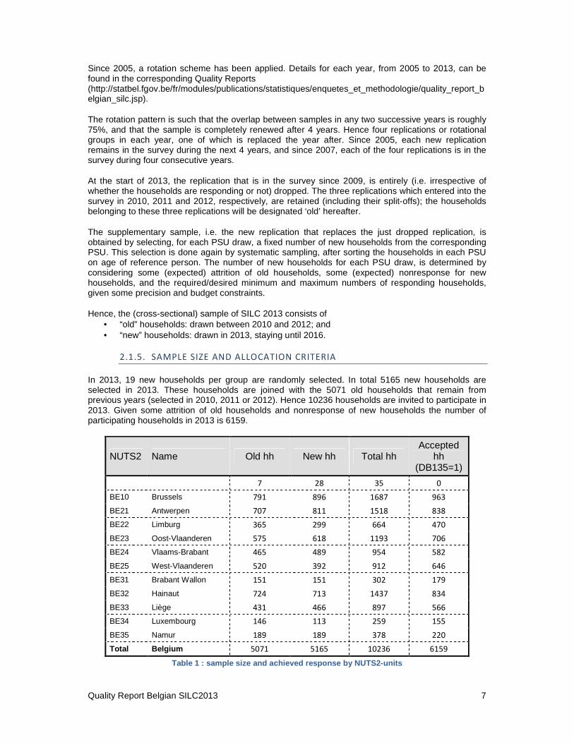
In 2013, 19 new households per group are randomly selected. In total 5165 new households are selected in 2013. These households are joined with the 5071 old households that remain from previous years (selected in 2010, 2011 or 2012). Hence 10236 households are invited to participate in 2013. Given some attrition of old households and nonresponse of new households the number of participating households in 2013 is 6159.
NUTS2 Name Old hh New hh Total hh Accepted
hh (DB135=1)
7 28 35 0
BE10 Brussels 791 896 1687 963
BE21 Antwerpen 707 811 1518 838
BE22 Limburg 365 299 664 470
BE23 Oost-Vlaanderen 575 618 1193 706
BE24 Vlaams-Brabant 465 489 954 582
BE25 West-Vlaanderen 520 392 912 646
BE31 Brabant Wallon 151 151 302 179
BE32 Hainaut 724 713 1437 834
BE33 Liège 431 466 897 566
BE34 Luxembourg 146 113 259 155
BE35 Namur 189 189 378 220
Total Belgium 5071 5165 10236 6159
Table 1 : sample size and achieved response by NUTS 2-units

Quality Report Belgian SILC2013 8
2.1.6. SAMPLE DISTRIBUTION OVER TIME
2.1.7. SUBSTITUTIONS
No substitution was applied in our survey.
2.1.8. WEIGHTINGS
Recall that, for the first year of the panel (=SILC 2004 in Belgium), the computation of weights involved three stages (described in 134-04):
- initial weights
- weights corrected for nonresponse
- final (calibrated) weights.
For 2013, a distinction has to be made between
“old” households i.e. households that contain at least one sample person who took part in 2012, and had to be surveyed again in 2013 according to the rotation and tracing rules (excluding the outgoing fourth) (household composition may have changed, whence quotations marks)
“new” households i.e. households that were drawn for the first time in 2013, among those households not containing any sample person already drawn before.
This distinction pertains to initial weights and nonresponse correction :
- Since the “old” households are selected indirectly from the 2010, 2011 or 2012 samples, and household composition may have changed, some kind of “weight sharing” must be applied to determine the (2013) initial weights, or rather base weights. On the other hand, “new” households have their own inclusion probability, whose inverse gives the initial weights;
- For the “old” households, (2013) nonresponse=attrition can be linked with (2012) SILC information. For the “new” households, all we can rely upon to explain initial nonresponse is auxiliary information from the Population Register (household size, urban/rural character) and the Financial Statistics (median fiscal income by municipality:)
On the other hand,
- Calibration can be done together for “old” and “new” households. With respect to our 2004 model, we decided in 2005 to relax the constraints (basically, calibrating at NUTS1-level instead of NUTS2), in order to decrease the standard deviation of weights.
This introduces the following sections :
- Initial weights for the new households
- Nonresponse correction for the new households
- Base weights for the old households
- Attrition correction for the old households
- Calibration (all households)
2.1.8.1. INITIAL WEIGHTS FOR THE NEW HOUSEHOLDS

Quality Report Belgian SILC2013 9
Belgium chose to draw the Primary Sampling Units (= municipalities or parts thereof) “forever”, and to rotate the Secondary Sampling Units (=households) within the selected PSU’s.
The 2004 PPS two-stage sampling design was self-weighting within each stratum h: x denoting any households in municipality X), we had (in 2004)
P (x drawn) = P(x drawn|X drawn) . P(X drawn) = nh/NX . NX/Nh . gh = nh/NH . gh, where
nh denotes the number of households to be drawn in the (selected) PSU (viz. 40)
NX the number of households in the PSU (in 2004)
Nh the number of households in the stratum (in 2004)
gh the number of PSU’s drawn in the stratum.
(This is an oversimplification, since PSU are drawn with repetition; the selection probability for a PSU should be replaced by the expectation of selection multiplicity, and the term 40 by a multiple depending on the selection multiplicity…but the idea is the same).
In 2013, the picture has become
P (x drawn) = P(x drawn|X drawn) . P(X drawn) = mh/MX . NX/Nh . gh, where
mh is the number of households to be drawn in the (selected) PSU (depending on h)
MX is the number of households in the PSU (in 2013)
The factor NX/MX indicates the increase-decrease in inclusion probabilities in PSU X (still assuming X has been drawn) between 2013 and 2004.
Now it would seem logical to replace NX by a smaller number, to account for the households1 already drawn in previous years (from 2004) whence immunized from being drawn again in 2013.
However, the following argument shows that (assuming momentarily that X has been drawn and that the population figures NX and MX remain stable) matters are not so easy:
P(x drawn in 2013) =
(P(x drawn in 2013 |x drawn before) . P(x drawn before)) +
(P(drawn in 2013 |x not drawn before) . P(x not drawn before),
the first term vanishes and the second equals nh/(MX-b). (NX-b)/Nh, where b denotes the number of hh already drawn; since both fraction terms are much larger than b (at least 900 in all selected PSU’s), the ratio (NX-b)/(MX-b) is (close to 1, and) very close to NX/MX. Since the term b is an approximation anyway, we chose to stick to mh/MX . NX/Nh. gh as inclusion probabilities, and its inverse for initial weights INIwei=DB080 . Note that, with this concept of DB080, the “new” hh correspond to the total Belgian population (some 4,5 millions private hh); before calibrating, theses weights will be scaled down “to make room” for the old hh; recovering the strange hh means that the sum of the pre-calibration weights will be slightly larger than 4,5 millions (average of g-weights slightly less than 1)
1 Perhaps a bit less (households that vanished already subtracted) or a bit more (split households, both
components of which stayed in PSU, should be subtracted twice)
Quality Report Belgian SILC2013 10
2.1.8.2. NONRESPONSE CORRECTION FOR THE NEW HOUSEHOLDS
Following Eurostat’s suggestion (see Document 065, WEIGHTING II. WEIGHTING FOR THE FIRST YEAR OF EACH SUB-SAMPLE), we replaced the homogeneous response groups (based on household size crossed with urbanity) ratio by a multiple regression model (based on the same dummy variables). By “responding”, we mean only those households whose results were accepted (DB135=1). Since 2009 we used logistic regression.
The file was split by NUTS1 and the following variables were used
- Everywhere: Household size, recoded into the four values “one”, “two”, “three” and “four or more” (so three dummies)
- Out of Brussels: DB100 = urbanity
- In Brussels = BE10: median fiscal income of municipality.
The regression produced a new variable “expresp”, allowing us to define
- NRwei = INIwei/expresp
2.1.8.3. ATTRITION FOR THE OLD HOUSEHOLDS
Before “sharing” the 2012 weights, a correction for attrition should be introduced. This year, we elected to perform this correction at the level of individuals, since a 2012 sample person either stays in the panel or leaves it (rotated out, left population, noncontact, refusal or inability to respond, while the structure of a household can change. Note that all household characteristics (e.g. HH021) can be distributed to the members.
We separated the “Children” (for which only basic personal information from the R-file and the distributed H-file is available) from the “Adults” (present in the 2012 P-file as well), i.e. those persons born in 1997 or before.
In the children’s model, the following predictors (all, except the last, from the 2012 file – although this does not matter much for group A) were used, grouped by type :
- individual demographic information: age from RB080, sex = RB090,
- housing information: dwelling type = HH010 and tenure = HH020
- household type: a limited number of dummies, as there is at least one dependent child;
- monetary indicators: we refrained from taking the equivalised income (outliers), but took a transform of it, as well as the dummy “poor or not” and the subjective ability to make ends meet = HS120
- sampling and rotation: number of years in panel (from DB075) and urbanisation (=DB100)
- one variable (paradata) related to fieldwork in 2011 (computed from HB040 and HB050)
For the adults, the same predictors were used, and moreover :
- variables from the P-file (related to education level and health);
- country of birth (dummy Belgium Yes/No)
were integrated.
We used logistic regression.

Quality Report Belgian SILC2013 11
2.1.8.4. WEIGHT SHARING
We followed Eurostat’s recommendation "EU-SILC weighting procedures: an outline" and shared the calibrated 2012 weights, after correcting for attrition (instead of the initial weights, see Lavallée).
This can be illustrated by an imaginary example, dealing simultaneously with fusions (persons A&B in same 2012 hh, C in another 2012 hh, so “fusion” in the sense of DB110 occurs), new members (a baby like E or already in population like D); we focus on the 2013 hh, what happened to those who co-resided with A and B or with C in 2012 (left or split) is irrelevant!
Note that:
- RB050 = weight 2012: same for A & B, vacuous for D and E
- Newi: in general a bit larger than RB050; A’s differs from B’s (attrition correction at individual level)
- Somwe = 950+1000+850 involves only A, B and C
- Weiind: = ¼ * somwe (A B C D : four contribute to the denominator)2
Person in 2013 hh A B C D E
RB110 (2013) 1 1 2 3 4
RB050 (weight 2012) 800 800 600 --- ---
Newi = Weight 2013 (after attrition correction) 950 1000 850 --- ---
Somwe (sum Newi over 2013 hh) 2800 2800 2800 2800 2800
Weiind 700 700 700 700 700
Table 2 : illustration weight sharing
Weiind will be injected as “initial” weight in the final calibration job.
2.1.8.5. CALIBRATION
We first put the pieces together: weiind is defined as:
- (new = started in 2013) :
initial weight, corrected for initial nonresponse, scaled, see 2.1.8.1)
- (old = took part in 2012) :
2012 weight, corrected for attrition and weight sharing if necessary, see 2.1.8.4)
- (back = did not take part in 2012 but before) :
2 Do we abide by the Eurostat rules (starting from base weights, it is unclear whether “their” attrition correction precedes or follows weight sharing) ? There remain some additional categories of persons to be considered:
- Children born to sample women. They receive the weight of the mother (this assumes that the baby belongs to his/her mother’s hh)
- Persons moving into sample households from outside the survey population. They receive the average of base weights of existing household members (vacuous here, as RB110 enables us to identify the newborns, but not the immigrants or the –few- persons moving from a collective to a private hh)
- Persons moving into sample households from other non-sample households in the population – these are “co-residents” and are given zero base weight.
Quality Report Belgian SILC2013 12
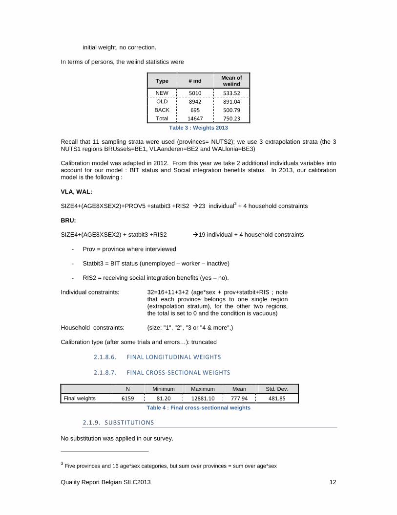
initial weight, no correction.
In terms of persons, the weiind statistics were
Type # ind Mean of weiind
NEW 5010 533.52
OLD 8942 891.04
BACK 695 500.79
Total 14647 750.23
Table 3 : Weights 2013
Recall that 11 sampling strata were used (provinces= NUTS2); we use 3 extrapolation strata (the 3 NUTS1 regions BRUssels=BE1, VLAanderen=BE2 and WALlonia=BE3)
Calibration model was adapted in 2012. From this year we take 2 additional individuals variables into account for our model : BIT status and Social integration benefits status. In 2013, our calibration model is the following :
VLA, WAL:
SIZE4+(AGE8XSEX2)+PROV5 +statbit3 +RIS2 �23 individual3 + 4 household constraints
BRU:
SIZE4+(AGE8XSEX2) + statbit3 +RIS2 �19 individual + 4 household constraints
- Prov = province where interviewed
- Statbit3 = BIT status (unemployed – worker – inactive)
- RIS2 = receiving social integration benefits (yes – no).
Individual constraints:
32=16+11+3+2 (age*sex + prov+statbit+RIS ; note that each province belongs to one single region (extrapolation stratum), for the other two regions, the total is set to 0 and the condition is vacuous)
Household constraints: (size: "1", "2", "3 or "4 & more",)
Calibration type (after some trials and errors…): truncated
2.1.8.6. FINAL LONGITUDINAL WEIGHTS
2.1.8.7. FINAL CROSS-SECTIONAL WEIGHTS
N Minimum Maximum Mean Std. Dev.
Final weights 6159 81.20 12881.10 777.94 481.85
Table 4 : Final cross-sectionnal weights
2.1.9. SUBSTITUTIONS
No substitution was applied in our survey.
3 Five provinces and 16 age*sex categories, but sum over provinces = sum over age*sex

Quality Report Belgian SILC2013 13
2.2. SAMPLING ERRORS
2.2.1. STANDARD ERRORS AND EFFECTIVE SAMPLE SIZE
In Annex we will present an overview of the standard errors for the common cross-sectional EU indicators and equivalised disposable income.
An overview of the achieved sample size for the ‘Laeken indicators’ and equivalised disposable income can be found in Table 15 of §2.3.3.6.
The design effect for the Median equivalised disposable income = 1.14.
There is no unbiased estimator of the design variance for SYSPPS with replacement sampling. The large PSU are selected with probability 1, but may not be considered as self-representative, because the number of groups selected is random, and the sum of the sampling weights of selected household do not equal PSU size.
Standard errors are estimated by jackknife repeated replication (JRR) method. The clusters are the groups, the strata made by two (or three) groups, using sampling order.
2.3. NON-SAMPLING ERRORS
2.3.1. SAMPLING FRAME AND COVERAGE ERRORS
The sampling frame is the Central Population Register. This Register includes all private households and their current members residing in the territory. Persons living in collective households and in institutions are excluded from the target population.
The Central Population Register of 1 February was used.
Updating actions: Central Population Register is updated two times during a month. The changes were communicated to the interviewers.
As there was a period of one month between the drawing of households and the survey itself, over-coverage, under-coverage and misclassification could be happen.
Over-coverage: Persons who died before the survey. Households who moved outside Belgium before the survey. Address is not the principal residence.
Under-coverage: Immigrants who came in Belgium before the survey. Persons who moved from a household to create a new household. Diplomats exempt from an inscription in the national register. Refugees on a waiting list.
Misclassification: Household who moved from a region in Belgium to another region of Belgium.
The size of coverage errors is not available but it was obviously small.
2.3.2. MEASUREMENT AND PROCESSING ERRORS
2.3.2.1. MEASUREMENT ERRORS
Measurement errors can occur from different sources, such as the survey instrument, the information system, the interviewer, the mode of collection (CAPI interview). We describe here a few elements by which possible measurement errors can be detected or which show on the other side the efforts taken to avoid as much as possible measurement errors.
Quality Report Belgian SILC2013 14
• Questionnaire construction
The questionnaire of the SILC2013 survey is the result of several steps:
For building up the questionnaire we took the blue print questionnaire of Eurostat as the basis (documents SILC055, SILC065 and EU-SILC65/02 Addendum II). The order of the questions and the groups (themes of) questions is taken from this blue print. The majority of the questions are almost literally copied (and translated), other questions are changed, however, because experiences in Belgium gave better results posing the questions in another way (The first questionnaires were developed in collaboration with the universities that have the experience of the ECHP/PSBH project in Belgium).
After each survey an evaluation of the questionnaire was made (detection of the problematic or difficult to answer questions based on the comments of the interviewers and on a study of the item non-response). When building up the SILC2013 questionnaire we took account of this evaluation.
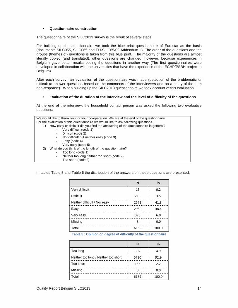
• Evaluation of the duration of the interview and the level of difficulty of the questions
At the end of the interview, the household contact person was asked the following two evaluative questions:
We would like to thank you for your co-operation. We are at the end of the questionnaire. For the evaluation of this questionnaire we would like to ask following questions.
1) How easy or difficult did you find the answering of the questionnaire in general? - Very difficult (code 1) - Difficult (code 2) - Not difficult but neither easy (code 3) - Easy (code 4) - Very easy (code 5)
2) What do you think of the length of the questionnaire? - Too long (code 1) - Neither too long neither too short (code 2) - Too short (code 3)
In tables Table 5 and Table 6 the distribution of the answers on these questions are presented.
N %
Very difficult 15 0.2
Difficult 218 3.5
Neither difficult / Nor easy 2573 41.8
Easy 2980 48.4
Very easy 370 6.0
Missing 3 0.0
Total 6159 100.0
Table 5 : Opinion on degree of difficulty of the qu estionnaire
N %
Too long 302 4.9
Neither too long / Neither too short 5720 92.9
Too short 135 2.2
Missing 0 0.0
Total 6159 100.0

Quality Report Belgian SILC2013 15
Table 6 : Opinion on the duration of the interview
For the majority of the participating households (54.4%), the questions were easy or very easy to interpret (57.2% in 2012). For 92.9% of the households the interview was neither too long, nor too short. This figure is similar to 2012 (93.5%).
As an evaluation after the survey we have sent the households and the interviewers each a different evaluation questionnaire.
• Mismatch in time between household composition and household income (see also §3.1)
A number of inconsistencies result from a mismatch between the composition of the household at the moment of the interview (between April and November of year x) and the income of the previous year (year x-1).
This mismatch can bias the measurement of poverty status in several ways. For example:
Persons who were full-time students in year x-1 (and depending on their parents), but were employed at the time of the interview (and living independently in a one person household for example) will report an income equal to 0 in year x-1 and will be wrongly classified as a poor household.
Other examples can also occur for persons where the household composition changed:
For a housewife who was married in year x-1, but divorced and is working at the time of the survey there will also be a mismatch
For a household which received family allowances for a student in year x-1, but where the student is no longer part of the household in year x there will also be a mismatch
For a household with a person working in year x-1, but retired at the moment of the survey (in year x) a mismatch will also occur. Take notice of the fact that, as the examples show the bias can go in both directions: under and over reporting of income. In each one of the examples, the choice to situate the income reference period in the past is the cause, however.
• Error in the routing
In 2013 there was a routing error in the way to compute the time taken by individuals to fill questionnaires.
• Interview training (Number of training days and information on the intensity and efficiency of interview training)
Overall we had the impression that the working-experience of the interviewers with EU-SILC starts to pay of. All new interviewers have to follow a two day formation. All trained interviewers followed a formation for an hour and half.
They both had to complete a test-interview before they could download their data. So we can be sure they can completely manage the use of the PC and that they know the questionnaire before they go on the field.
A training group for new interviewers consisted of minimum 5 to maximum 20 interviewers, and according to the size of the training group there were 1 or 2 trainers.
Even though the accent was given to the practical side of the training (getting to know the questions and mastering the CAPI-program by imitating interview situations), three manuals were distributed and explained during the training:

Quality Report Belgian SILC2013 16
A general manual (‘Manuel general aux enquêteurs’) containing information about the objectives of the survey, the organisation of the survey, legal and administrative aspects around the survey, fieldwork aspect (how to contact the household, how to introduce oneself, who answers which questions, time delays, …) and the content of the questionnaires.
A second manual (‘Manuel contenu’) with all kinds of additional explanations and examples for certain questions/answers.
A third manual (‘Manuel CAPI’) about the use of the portable PC for the SILC Computer Assisted Personal Interviews and about the data entry program itself.
The first day of the training there was half a day for learning about and discussing the first two manuals. In the afternoon the trainees received their laptop and got to know the survey and the tool to carry out the interview in practice. One test-interview was simulated collectively. The second day of the training a small part of the time was dedicated to testing to send the data electronically after carrying out the interview. All the rest of the day interviewers practiced several interviews and interview situations with each other on the basis of household profiles that were given. There was also a lot of time for questions and discussions in between these test-interviews.
At the end of the training sessions the instructors had a good image on the degree in which each interviewer ameliorated during the training and on the degree in which they mastered the work. For certain interviewers two days of training was more than enough to master the work, for others it was necessary that they practiced some more at home on specific aspects of carrying out this survey (for example using of the CAPI-program itself, working on the content of the survey, …). They were recommended to do so before carrying out their first real interview. They were often also recommended to start interviewing one-person households.
A training group for trained interviewers consisted maximum 30 interviewers with two trainers. The accent was also given on the content: questions that changed, the module 2011 and questions, which are misunderstood by the interviewers. We made an extra manual for trained interviewers. The trained interviewers obtained four manuals:
- A general manual (‘Manuel general aux enquêteurs’) containing information about the objectives of the survey, the organisation of the survey, legal and administrative aspects around the survey, fieldwork aspect (how to contact the household, how to introduce oneself, who answers which questions, time delays, …) and the content of the questionnaires.
- A second manual (‘Manuel contenu’) with all kinds of additional explanations and examples for certain questions/answers.
- A third manual (‘Manuel CAPI’) about the use of the portable PC for the SILC Computer Assisted Personal Interviews and about the data entry program itself.
- A fourth manual (‘Modifications du questionnaire : module 2013) about the module, changed questions and questions misunderstood by the interviewers.
• Skills testing before starting the fieldwork
Interviewers were selected from the interviewer database that Statistics Belgium has centralised for all the survey’s that are carried out by the institute. For each interviewer a basic curriculum vitae is present in the database (mentioning for example for which surveys they have experience, their language knowledge, their knowledge of pc, …). A specific unit at Statistics Belgium (‘Unité Corps Enquêteurs’) is occupied with the selection of the interviewers for each survey; they have good contact with and knowledge of the interviewers. They try to find the best interviewer for each of the geographical areas to cover for SILC. This is not always an easy task because for certain geographical areas several interviewers are candidate, but for other geographical unit there are few or no candidates. Note that interviewers in Belgium most often carry out this work as a second or casual occupation.

Quality Report Belgian SILC2013 17
• Skills control during the fieldwork
During the fieldwork we controlled the work of the interviewers by looking at some of their completed questionnaires. We gave extra attention to all new interviewers and to some trained interviewers that we suspected to be less accurate. Remarks (positive as negative) resulting from these controls were immediately communicated to the interviewer so they could improve their way of working and interviewing.
• Number of households by interviewer
Groups of secondary units consisted of about 35 households, depending on the strata. Most of the interviewers had one group of households. Nevertheless several interviewers also had more groups:
N
interviewers with 1 group: 44
interviewers with 2 groups: 39
interviewers with 3 groups: 25
interviewers with 4 groups: 19
interviewers with 5 groups: 8
interviewers with 6 groups: 5
interviewers with 7 groups: 1
interviewers with 8 groups: 1
interviewers with 10 groups: 2
Table 7 : Number of groups by interviewer
2.3.2.2. PROCESSING ERRORS
Belgium used the CAPI–method to interview the persons. The questionnaire was programmed in Blaise. So processing errors due to data entry (from a written to an electronic format) were reduced to a minimum.
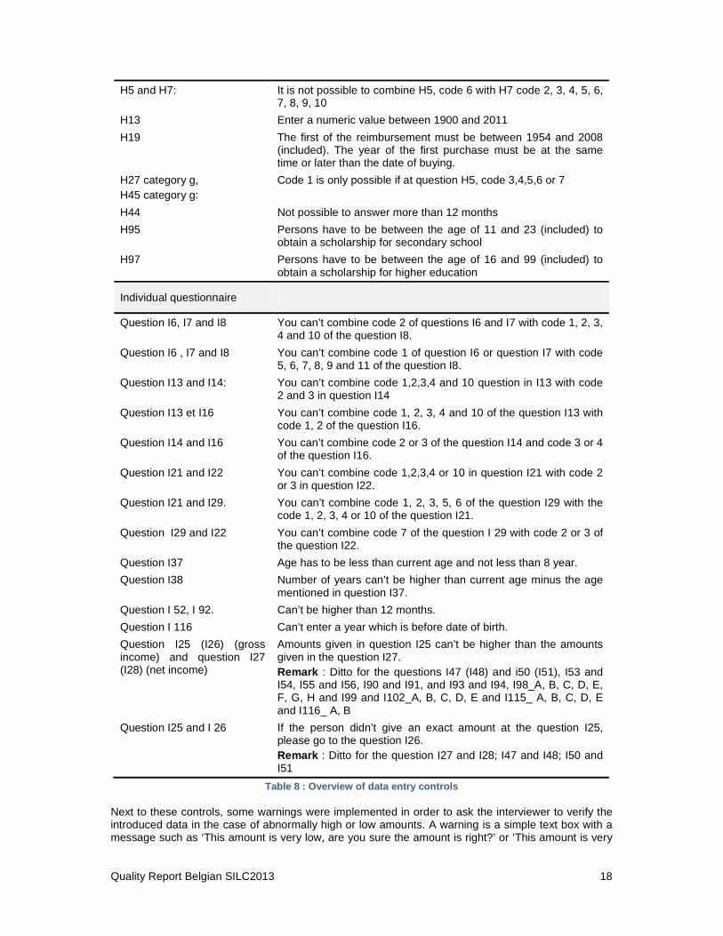
Statistics Belgium programmes several data entry and coding controls in the Blaise program. Below an overview of both data entry and coding controls is presented.
• Data entry controls
Question number Control
Contact form
Column 21, 22, 23 and 24
You can’t combine father, mother or being spouse with ‘being younger than 12 years”.
Column 8,21 and 22
It’s not possible to combine being ‘female’ and being ‘father’. It’s not possible to combine being ‘male’ and being ‘mother’.
Column 21 and 22 Mother and father have to be older than their children (and at least being older than 12 years).
Column 21, 22, 23, 24 Parents of the spouses or of the partners must be different.
Column 23, 24 You can’t mix ‘spouse ‘and ‘partner’. Must choose one of both for the couple.
Household questionnaire
Quality Report Belgian SILC2013 18
H5 and H7: It is not possible to combine H5, code 6 with H7 code 2, 3, 4, 5, 6, 7, 8, 9, 10
H13 Enter a numeric value between 1900 and 2011
H19 The first of the reimbursement must be between 1954 and 2008 (included). The year of the first purchase must be at the same time or later than the date of buying.
H27 category g, H45 category g:
Code 1 is only possible if at question H5, code 3,4,5,6 or 7
H44 Not possible to answer more than 12 months
H95 Persons have to be between the age of 11 and 23 (included) to obtain a scholarship for secondary school
H97 Persons have to be between the age of 16 and 99 (included) to obtain a scholarship for higher education
Individual questionnaire
Question I6, I7 and I8 You can’t combine code 2 of questions I6 and I7 with code 1, 2, 3, 4 and 10 of the question I8.
Question I6 , I7 and I8 You can’t combine code 1 of question I6 or question I7 with code 5, 6, 7, 8, 9 and 11 of the question I8.
Question I13 and I14: You can’t combine code 1,2,3,4 and 10 question in I13 with code 2 and 3 in question I14
Question I13 et I16 You can’t combine code 1, 2, 3, 4 and 10 of the question I13 with code 1, 2 of the question I16.
Question I14 and I16 You can’t combine code 2 or 3 of the question I14 and code 3 or 4 of the question I16.
Question I21 and I22 You can’t combine code 1,2,3,4 or 10 in question I21 with code 2 or 3 in question I22.
Question I21 and I29. You can’t combine code 1, 2, 3, 5, 6 of the question I29 with the code 1, 2, 3, 4 or 10 of the question I21.
Question I29 and I22 You can’t combine code 7 of the question I 29 with code 2 or 3 of the question I22.
Question I37 Age has to be less than current age and not less than 8 year.
Question I38 Number of years can’t be higher than current age minus the age mentioned in question I37.
Question I 52, I 92. Can’t be higher than 12 months.
Question I 116 Can’t enter a year which is before date of birth.
Question I25 (I26) (gross income) and question I27 (I28) (net income)
Amounts given in question I25 can’t be higher than the amounts given in the question I27. Remark : Ditto for the questions I47 (I48) and i50 (I51), I53 and I54, I55 and I56, I90 and I91, and I93 and I94, I98_A, B, C, D, E, F, G, H and I99 and I102_A, B, C, D, E and I115_ A, B, C, D, E and I116_ A, B
Question I25 and I 26 If the person didn’t give an exact amount at the question I25, please go to the question I26. Remark : Ditto for the question I27 and I28; I47 and I48; I50 and I51
Table 8 : Overview of data entry controls
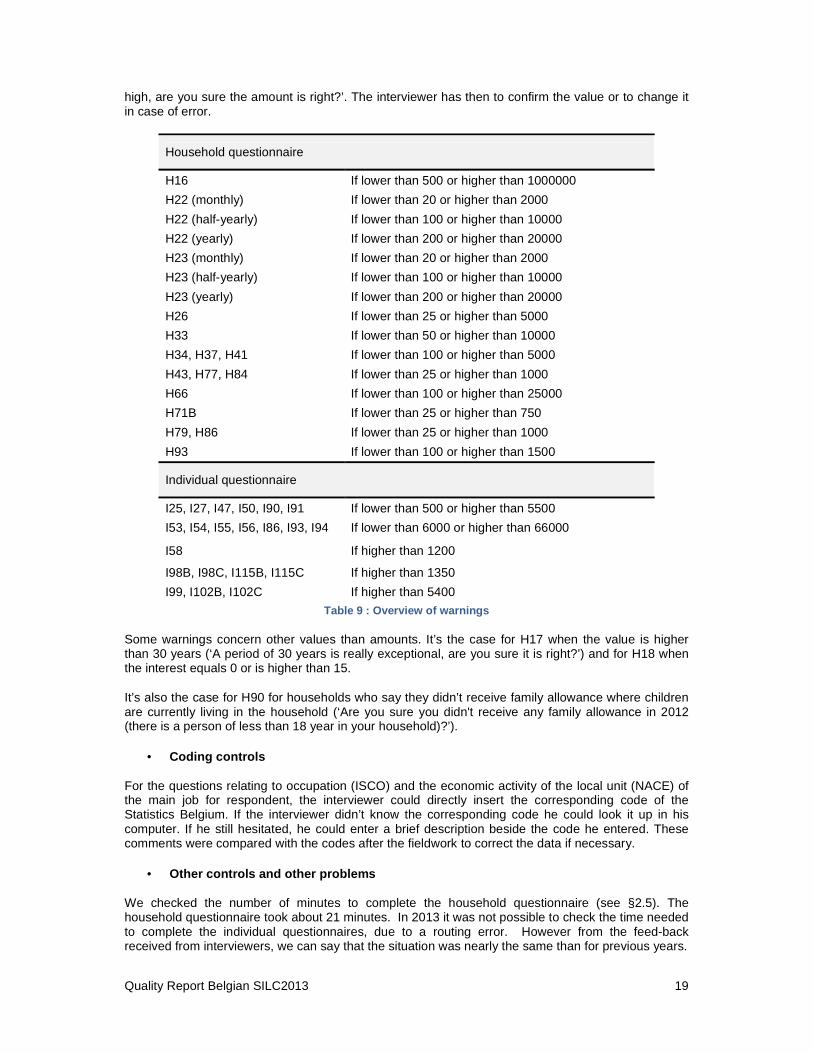
Next to these controls, some warnings were implemented in order to ask the interviewer to verify the introduced data in the case of abnormally high or low amounts. A warning is a simple text box with a message such as ‘This amount is very low, are you sure the amount is right?’ or ‘This amount is very
Quality Report Belgian SILC2013 19
high, are you sure the amount is right?’. The interviewer has then to confirm the value or to change it in case of error.
Household questionnaire
H16 If lower than 500 or higher than 1000000
H22 (monthly) If lower than 20 or higher than 2000
H22 (half-yearly) If lower than 100 or higher than 10000
H22 (yearly) If lower than 200 or higher than 20000
H23 (monthly) If lower than 20 or higher than 2000
H23 (half-yearly) If lower than 100 or higher than 10000
H23 (yearly) If lower than 200 or higher than 20000
H26 If lower than 25 or higher than 5000
H33 If lower than 50 or higher than 10000
H34, H37, H41 If lower than 100 or higher than 5000
H43, H77, H84 If lower than 25 or higher than 1000
H66 If lower than 100 or higher than 25000
H71B If lower than 25 or higher than 750
H79, H86 If lower than 25 or higher than 1000
H93 If lower than 100 or higher than 1500
Individual questionnaire
I25, I27, I47, I50, I90, I91 If lower than 500 or higher than 5500
I53, I54, I55, I56, I86, I93, I94 If lower than 6000 or higher than 66000
I58 If higher than 1200
I98B, I98C, I115B, I115C If higher than 1350
I99, I102B, I102C If higher than 5400
Table 9 : Overview of warnings
Some warnings concern other values than amounts. It’s the case for H17 when the value is higher than 30 years (‘A period of 30 years is really exceptional, are you sure it is right?’) and for H18 when the interest equals 0 or is higher than 15.
It’s also the case for H90 for households who say they didn’t receive family allowance where children are currently living in the household (‘Are you sure you didn't receive any family allowance in 2012 (there is a person of less than 18 year in your household)?’).
• Coding controls
For the questions relating to occupation (ISCO) and the economic activity of the local unit (NACE) of the main job for respondent, the interviewer could directly insert the corresponding code of the Statistics Belgium. If the interviewer didn’t know the corresponding code he could look it up in his computer. If he still hesitated, he could enter a brief description beside the code he entered. These comments were compared with the codes after the fieldwork to correct the data if necessary.
• Other controls and other problems
We checked the number of minutes to complete the household questionnaire (see §2.5). The household questionnaire took about 21 minutes. In 2013 it was not possible to check the time needed to complete the individual questionnaires, due to a routing error. However from the feed-back received from interviewers, we can say that the situation was nearly the same than for previous years.
Quality Report Belgian SILC2013 20
2.3.3. NON-RESPONSE ERRORS
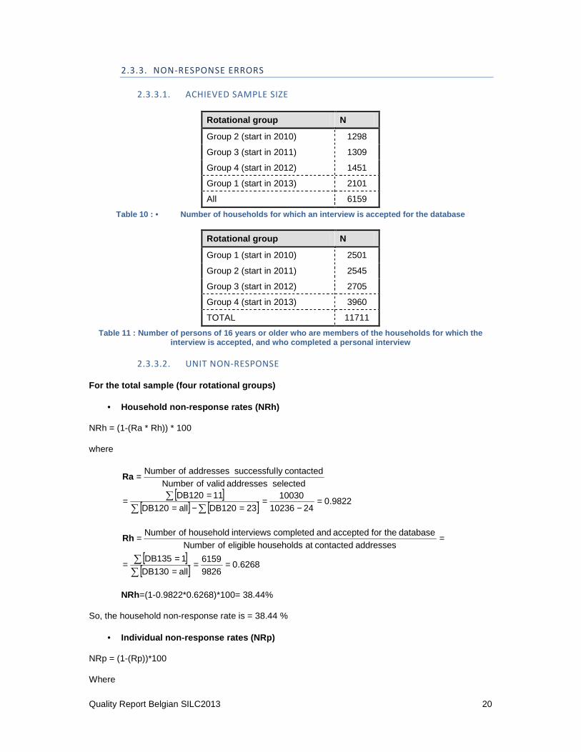
2.3.3.1. ACHIEVED SAMPLE SIZE
Rotational group N
Group 2 (start in 2010) 1298
Group 3 (start in 2011) 1309
Group 4 (start in 2012) 1451
Group 1 (start in 2013) 2101
All 6159
Table 10 : • Number of households for which an inte rview is accepted for the database
Rotational group N
Group 1 (start in 2010) 2501
Group 2 (start in 2011) 2545
Group 3 (start in 2012) 2705
Group 4 (start in 2013) 3960
TOTAL 11711
Table 11 : Number of persons of 16 years or older w ho are members of the households for which the interview is accepted, and who completed a personal interview
2.3.3.2. UNIT NON-RESPONSE
For the total sample (four rotational groups)
• Household non-response rates (NRh)
NRh = (1-(Ra * Rh)) * 100
where
[ ][ ] [ ] 9822.0
241023610030
23DB120allDB12011DB120
selected addresses valid of Numbercontactedly successful addresses of Number
=−
==−=
==
=
∑ ∑
∑
Ra
[ ][ ] 6268.0
98266159
allDB130
1DB135
addresses contacted at households eligible of Numberdatabase the for accepted and completed interviews household of Number
====
=
==
∑
∑
Rh
NRh=(1-0.9822*0.6268)*100= 38.44%
So, the household non-response rate is = 38.44 %
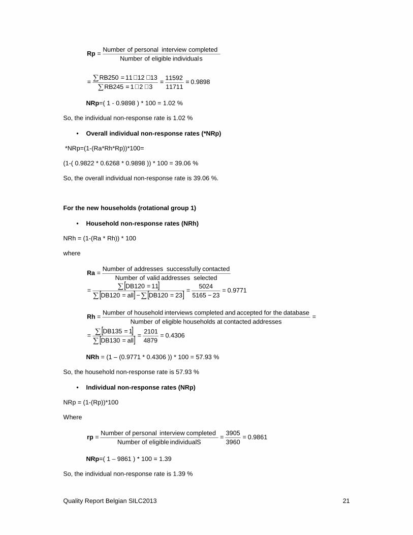
• Individual non-response rates (NRp)
NRp = (1-(Rp))*100
Where
Quality Report Belgian SILC2013 21
9898.01171111592
321RB245
131211RB250
sindividual eligible of Number completedinterview personal of Number
==++=++=
=
=
∑
∑
Rp
NRp=( 1 - 0.9898 ) * 100 = 1.02 %
So, the individual non-response rate is 1.02 %
• Overall individual non-response rates (*NRp)
*NRp=(1-(Ra*Rh*Rp))*100=
(1-( 0.9822 * 0.6268 * 0.9898 )) * 100 = 39.06 %
So, the overall individual non-response rate is 39.06 %.
For the new households (rotational group 1)
• Household non-response rates (NRh)
NRh = (1-(Ra * Rh)) * 100
where
[ ][ ] [ ] 9771.0
2351655024
23DB120allDB12011DB120
selected addresses valid of Numbercontactedly successful addresses of Number
=−
==−=
==
=
∑ ∑
∑
Ra
[ ][ ] 4306.0
48792101
allDB130
1DB135
addresses contacted at households eligible of Numberdatabase the for accepted and completed interviews household of Number
====
=
==
∑
∑
Rh
NRh = (1 – (0.9771 * 0.4306 )) * 100 = 57.93 %
So, the household non-response rate is 57.93 %
• Individual non-response rates (NRp)
NRp = (1-(Rp))*100
Where
9861.039603905
Sindividual eligible of Number completedinterview personal of Number ===rp
NRp=( 1 – 9861 ) * 100 = 1.39
So, the individual non-response rate is 1.39 %
Quality Report Belgian SILC2013 22
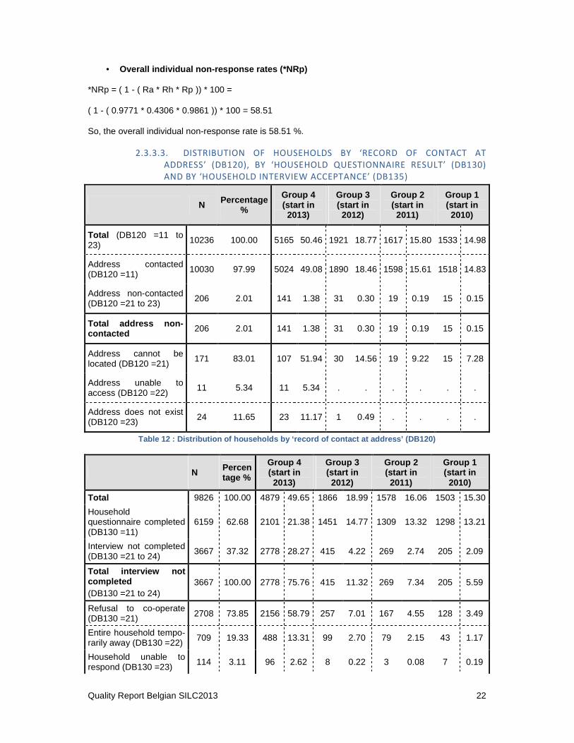
• Overall individual non-response rates (*NRp)
*NRp = ( 1 - ( Ra * Rh * Rp )) * 100 =
( 1 - ( 0.9771 * 0.4306 * 0.9861 )) * 100 = 58.51
So, the overall individual non-response rate is 58.51 %.
2.3.3.3. DISTRIBUTION OF HOUSEHOLDS BY ‘RECORD OF CONTACT AT
ADDRESS’ (DB120), BY ‘HOUSEHOLD QUESTIONNAIRE RESULT’ (DB130)
AND BY ‘HOUSEHOLD INTERVIEW ACCEPTANCE’ (DB135)
N Percentage %
Group 4 (start in 2013)
Group 3 (start in 2012)
Group 2 (start in 2011)
Group 1 (start in 2010)
Total (DB120 =11 to 23) 10236 100.00 5165 50.46 1921 18.77 1617 15.80 1533 14.98
Address contacted (DB120 =11) 10030 97.99 5024 49.08 1890 18.46 1598 15.61 1518 14.83
Address non-contacted (DB120 =21 to 23) 206 2.01 141 1.38 31 0.30 19 0.19 15 0.15
Total address non-contacted 206 2.01 141 1.38 31 0.30 19 0.19 15 0.15
Address cannot be located (DB120 =21) 171 83.01 107 51.94 30 14.56 19 9.22 15 7.28
Address unable to access (DB120 =22)
11 5.34 11 5.34 . . . . . .
Address does not exist (DB120 =23) 24 11.65 23 11.17 1 0.49 . . . .
Table 12 : Distribution of households by ‘record of contact at address’ (DB120)
N Percentage %
Group 4 (start in 2013)
Group 3 (start in 2012)
Group 2 (start in 2011)
Group 1 (start in
2010)
Total 9826 100.00 4879 49.65 1866 18.99 1578 16.06 1503 15.30
Household questionnaire completed (DB130 =11)
6159 62.68 2101 21.38 1451 14.77 1309 13.32 1298 13.21
Interview not completed (DB130 =21 to 24) 3667 37.32 2778 28.27 415 4.22 269 2.74 205 2.09
Total interview not completed (DB130 =21 to 24)
3667 100.00 2778 75.76 415 11.32 269 7.34 205 5.59
Refusal to co-operate (DB130 =21) 2708 73.85 2156 58.79 257 7.01 167 4.55 128 3.49
Entire household tempo-rarily away (DB130 =22) 709 19.33 488 13.31 99 2.70 79 2.15 43 1.17
Household unable to respond (DB130 =23) 114 3.11 96 2.62 8 0.22 3 0.08 7 0.19

Quality Report Belgian SILC2013 23
Unable to respond (DB130 = 24 136 3.71 38 1.04 51 1.39 20 0.55 27 0.74
Household questionnaire completed (DB135=1+2)
6159 100.00 2101 34.11 1451 23.56 1309 21.25 1298 21.07
Interview accepted for database (DB135=1) 6159 100.00 2101 34.11 1451 23.56 1309 21.25 1298 21.07
Interview rejected (DB135=2) . . . . . . . . . .
Table 13 : Distribution of households by ‘household questionnaire result’ (DB130) and by ‘household interview acceptance’ (DB135)
Longitudinal non response rate for the 3 groups to follow:
( 1 - ( 0.9874 * 0.8203 * 0.9917 ) * 100) = 19.67
2.3.3.4. DISTRIBUTION OF SUBSTITUTED UNITS
No substitution was applied in our survey.
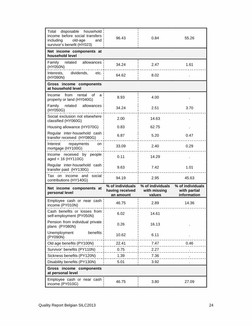
2.3.3.5. ITEM NON-RESPONSE
In Table 14, an overview of the item non-response for all income variables is presented. The percentage households having received an amount, the percentage of households with missing values and the percentage of households with partial information is calculated.
These percentages are calculated as follows:
% of households having received an amount : number of households (or persons) who have received something (yes to a filter) / total
% of households with missing values : number of households (or persons) who said that they have received something but did not give any amount (no partial information) / number of households (or persons) who have received something (yes to a filter)
% of households with partial information: number of households (or persons – depending on the source of the variable – household file HY or personal file PY ) who said that they have received something but gave partial information (amounts were not given for all components) / number of households (or persons) who have received something (yes to a filter)
Item non-response
% of households
having received an amount
% of households with missing
values
% of households with partial information
Total gross household income (HY010) 99.77 10.74 40.65
Total disposable household income (HY020) 99.84 4.13 51.16
Total disposable household income before social transfers except old-age and survivor’s benefits (HY022)
97.99 3.21 52.63
Quality Report Belgian SILC2013 24
Total disposable household income before social transfers including old-age and survivor’s benefit (HY023)
96.43 0.84 55.26
Net income components at household level
Family related allowances (HY050N) 34.24 2.47 1.61
Interests, dividends, etc. (HY090N) 64.62 8.02 .
Gross income components at household level
Income from rental of a property or land (HY040G) 8.93 4.00 .
Family related allowances (HY050G) 34.24 2.51 3.70
Social exclusion not elsewhere classified (HY060G) 2.00 14.63 .
Housing allowance (HY070G) 0.83 62.75 .
Regular inter-household cash transfer received (HY080G) 6.87 5.20 0.47
Interest repayments on mortgage (HY100G) 33.09 2.40 0.29
Income received by people aged < 16 (HY110G) 0.11 14.29 .
Regular inter-household cash transfer paid (HY130G) 9.63 7.42 1.01
Tax on income and social contributions (HY140G) 94.19 2.95 45.63
Net income components at personal level
% of individuals having received
an amount
% of individuals with missing
values
% of individuals with partial information
Employee cash or near cash income (PY010N) 46.75 2.89 14.36
Cash benefits or losses from self-employment (PY050N) 6.02 14.61
Pension from individual private plans (PY080N) 0.26 16.13 .
Unemployment benefits (PY090N) 10.62 6.11 .
Old age benefits (PY100N) 22.41 7.47 0.46
Survivor’ benefits (PY110N) 0.75 2.27 .
Sickness benefits (PY120N) 1.39 7.36 .
Disability benefits (PY130N) 5.01 3.92 .
Gross income components at personal level
Employee cash or near cash income (PY010G)
46.75 3.80 27.09
Quality Report Belgian SILC2013 25
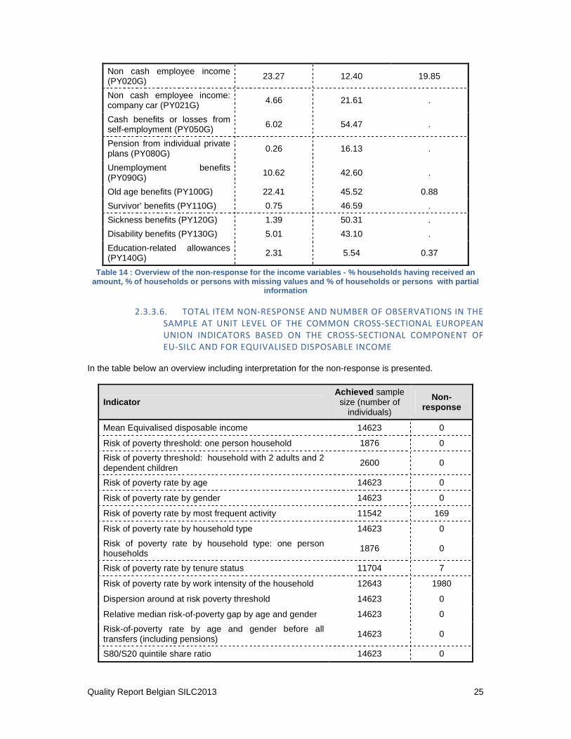
Non cash employee income (PY020G) 23.27 12.40 19.85
Non cash employee income: company car (PY021G) 4.66 21.61 .
Cash benefits or losses from self-employment (PY050G) 6.02 54.47 .
Pension from individual private plans (PY080G) 0.26 16.13 .
Unemployment benefits (PY090G) 10.62 42.60 .
Old age benefits (PY100G) 22.41 45.52 0.88
Survivor’ benefits (PY110G) 0.75 46.59 .
Sickness benefits (PY120G) 1.39 50.31 .
Disability benefits (PY130G) 5.01 43.10 .
Education-related allowances (PY140G) 2.31 5.54 0.37
Table 14 : Overview of the non-response for the inc ome variables - % households having received an amount, % of households or persons with missing val ues and % of households or persons with partial
information
2.3.3.6. TOTAL ITEM NON-RESPONSE AND NUMBER OF OBSERVATIONS IN THE
SAMPLE AT UNIT LEVEL OF THE COMMON CROSS-SECTIONAL EUROPEAN
UNION INDICATORS BASED ON THE CROSS-SECTIONAL COMPONENT OF
EU-SILC AND FOR EQUIVALISED DISPOSABLE INCOME
In the table below an overview including interpretation for the non-response is presented.
Indicator Achieved sample size (number of
individuals)
Non-response
Mean Equivalised disposable income 14623 0
Risk of poverty threshold: one person household 1876 0
Risk of poverty threshold: household with 2 adults and 2 dependent children
2600 0
Risk of poverty rate by age 14623 0
Risk of poverty rate by gender 14623 0
Risk of poverty rate by most frequent activity 11542 169
Risk of poverty rate by household type 14623 0
Risk of poverty rate by household type: one person households 1876 0
Risk of poverty rate by tenure status 11704 7
Risk of poverty rate by work intensity of the household 12643 1980
Dispersion around at risk poverty threshold 14623 0
Relative median risk-of-poverty gap by age and gender 14623 0
Risk-of-poverty rate by age and gender before all transfers (including pensions) 14623 0
S80/S20 quintile share ratio 14623 0
Quality Report Belgian SILC2013 26
Gini coefficient 14623 0
Table 15 : item non-response and number of observat ions at unit level of the common cross-sectional European Union indicators and for equivalised dispo sable income.
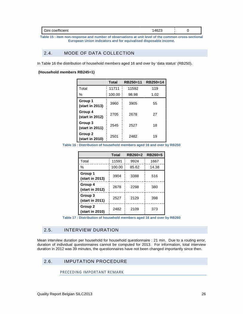
2.4. MODE OF DATA COLLECTION
In Table 16 the distribution of household members aged 16 and over by ‘data status’ (RB250).
(Household members RB245=1)
Total RB250=11 RB250=14
Total 11711 11592 119
% 100.00 98.98 1.02
Group 1 (start in 2013)
3960 3905 55
Group 4 (start in 2012)
2705 2678 27
Group 3 (start in 2011)
2545 2527 18
Group 2 (start in 2010)
2501 2482 19
Table 16 : Distribution of household members aged 1 6 and over by RB250
Total RB260=2 RB260=5
Total 11591 9924 1667
% 100.00 85.62 14.38
Group 1 (start in 2013)
3904 3388 516
Group 4 (start in 2012)
2678 2298 380
Group 3 (start in 2011)
2527 2129 398
Group 2 (start in 2010)
2482 2109 373
Table 17 : Distribution of household members aged 1 6 and over by RB260
2.5. INTERVIEW DURATION
Mean interview duration per household for household questionnaire : 21 min. Due to a routing error, duration of individual questionnaires cannot be computed for 2013. For information, total interview duration in 2012 was 39 minutes, the questionnaires have not been changed importantly since then.
2.6. IMPUTATION PROCEDURE
PRECEDING IMPORTANT REMARK

Quality Report Belgian SILC2013 27
In contrast to 2004 and as 2005 – from 2006 onwards (so also in 2013) the calendar question (i40 in the questionnaire) was presented to every respondent rather the only those who indicated that had been a change in their social-economic position. It enabled us to assess and check much thoroughly the link between the social-economic position and the income variables. Notably for the self-employed this resulted in a substantive number of cases (being identified as being self-employed) who would be otherwise (and who were to some extent in 2004) not identified as being self-employed. These cases mainly concern people in jobs ‘somewhere on the bridge’ between being self-employed and employee but who nevertheless indicated in the calendar that they were self-employed.
2.6.1. OVERALL STRATEGY: EMPHASIS ON INTERNAL INFORMATION AND
INTEGRATION OF OUTLIER DETECTION- , IMPUTATION- AND CONTROL-
PHASES.
Between 2012 and 2013 there was no major changes in our overall strategy.
2.6.1.1. EMPHASIS ON INTERNAL INFORMATION.
We can’t emphasise enough that to correct and impute our data (for any variable) we relied: a) as much as possible on internal information pres ent in the data itself b) on formal and legal sources of information and c) only as final resort turned to statistical procedures (random imputations for ex.)
2.6.1.2. AN INTEGRATED STRATEGY.
As it was the case for previous SILC-surveys we used from SILC-2013 again an ‘integrated approach’ to organise the detection of outliers and the imputations. Crucial to the understanding of our way of working are the concepts of what we call ‘vertical’ and ‘horizontal integration’.
By ‘vertical integration’ we mean that the phases of outlier detection and imputation were done together for each variable separately (1) rather than that both phases were done separately for all variables together (2). The differences between (1) – the way we did things for SILC 2004 - and (2) the way it was done for SILC 2003 – are subtle but nevertheless more than semantics, especially when combined with horizontal integration.
By horizontal integration we mean that information for each respondent on one variable was checked against information on another variable or another source. Information on the monthly gross income for example was – if both possible and applicable- checked with information on the net income, the yearly income, the current income (if no changes had occurred), the household income, other ‘proxi’- variables to income (status etc…) and very important external sources of information like legislation.
The interplay between what we call vertical and horizontal integration leads to a dynamic strategy: variables are checked for outliers and inconsistencies, variables are compared to each other and corrected, (corrected) variables are immediately imputed consistently to the information in other (also corrected) variables – and this several times repeated.
We believe that the emphasis of this strategy on consistency of internal information for respondents throughout the survey and the use of external sources of information (legislation) is a far more successful way of detecting outliers and imputing missing values compared to methods of screening for outliers entirely based on (univariate) distributional features of variables (box-plot methods for example) and imputation methods mainly based on statistical probability models (IVE for example).
OUTLIER DETECTION:
The shift in strategy also implies – of course - a shift in the techniques that are used. As far as the outlier detection concerns there is far less emphasis on univariate - purely distributional related methods like box-plots but more emphasis on inconsistency checks. For the income variables these checks were done in 2 ways: a) comparison of ratio’s between variables and b) comparison of the relative position of a respondent’s answer on one variable to its position on another variable.

Quality Report Belgian SILC2013 28
a) Comparison of ratio’s between variables:
Comparison of the ratio between two inputs on comparable income variables is a straightforward way to detect outliers. Atypical large or small ratios between gross and net variants of income variables are obviously an indication of ‘something being wrong’.
b) Comparison of relative positions on income varia bles:
The central issue in this procedure is the comparison of two income variables by comparison of the normal scores calculated for each case on both variables, after log-transformation. The log-transformation is necessary to normalize the otherwise poisson-distributed income variables.
The inputs of both comparable incomes are considered to be consistent if both normal scores are within predefined boundaries (for example -1,96 and 1,96) and/or the difference between the normal scores is limited (less than 1,96).
There is an indication of bias if the input of one of the incomes for a case is situated within ‘normal boundaries’ ( -1.96 – 1.96) but the other input is not and/or if the difference between the two normal scores differ substantially (>1.96). In fact, the entire procedure consist out of 4 steps:
- Identification of the variables to be compared. - Log-transformations, normality checks, calculation of means and standard deviations. - Calculation of normal scores. - Consistency control and identification of inconsistencies.
c) Other techniques :
There was explicitly more emphasis on the above techniques but this does not imply that the ‘conventional’ box-plot method was not used at all. In this method input outside the interval below were considered to be outliers:
[First Quartile – 1,5 * (Third Quartile – First Quartile) ; Third Quartile + 1,5 * (Third Quartile – First Quartile)]
Furthermore and as already mentioned, where applicable and usable legal maximums and minimums were also used to some extent.
Finally, we also checked for outliers via controls on a ‘case to case’ base in which we maximally used information of proxi-variables like professional status and other variables. In this process manifest errors in proxi- and/or other variables associated with the income variables were also removed/corrected (for example ‘the number of months’).
IMPUTATION
We did no longer make use of IVE. Instead we a) corrected (not imputed – in fact) a greater number of cases and if correction was not desirable or possible, but information on a directly comparable variable was present anyway (see section on internal information above), we b) resorted to direct imputation, via a regression model.
a) Corrections.
Corrections were also mainly done on basis of information in other comparable variables. Gross-net ratio of 12 - yearly income entered as monthly or vice versa - lead to simple corrections of the gross or the net, for example.
b) Regressions.
If correction was not desirable or possible but information on a directly comparable variable was present anyway, we resorted to direct imputation, via a regression model, of the variable for which input was missing. Below we describe how this was done for net –gross imputation, which were the

Quality Report Belgian SILC2013 29
most prevalent instances of that sort. The method was extended, however, to other imputations (imputations of the reference year income based on the current income, for example).
Missing values on gross income variables (PY010G, PY020G, … and components) were, if collected, imputed on the basis of the corresponding net variables (PY010N, PY020N, … and components). The implementation of this imputation procedure was quasi-similar for almost all (income) variables on which it was applied. The procedure implied 6-steps:
1) Identification of the ‘reference cases’ (both gross and net collected) and identification of the cases to be imputed (net collected – gross missing).
2) Calculation of the gross/net ratio for the reference cases. Cases with an extreme value on this ratio were excluded from further use in the procedure.
3) Curve estimation of the relation (regression model) between gross and net income. The best fitting model (linear, logarithmic, quadratic, exponential) was being implemented.
4) Implementation of the regression model for the reference cases to identify outliers.
5) Re-implementation of the regression model for the reference cases after removal of the outliers.
6) Actual imputation step: missing (gross) values are imputed on the basis of
a) net values and
b) the estimates for the relation between gross and net income assessed in the steps above.
In step 1 the cases of which both gross and net income were collected are identified. We refer to these cases as ‘reference cases’ (step 1). The relationship between their net and gross income serves as reference for the imputation of the gross incomes for the cases where only the net was collected (cases to be imputed).
To avoid bias in this imputation model atypical reference cases (both outliers and errors) were identified and removed at several steps in the procedure (step 2 and 4).
In step 2 (reference)cases for whom the ratio between gross and net income exceeded what can be considered typical for the taxation regime applicable to the income concerned, were excluded.
In the case of almost all variables the boundary value of this ratio was set at 2,5. This boundary was arbitrary chosen.
Scrutiny of the excluded cases, however, validates this value’s potential to discriminate between incomes which were subjected to real(istic) taxation and outliers or errors.
The latter category seldom counted more than a few percent of the total population in the survey and their gross/net ratio often exceeded the 2,5 considerably.
Further exploration also revealed that the exclusion of these cases from the procedure results in a dramatic increase of the fit of the regression model on which the imputation is based.
In step 4 outliers in the regression model were identified and removed using default regression diagnostics.
The underlying probability model of the net-gross relation was assessed with SAS regression model or SAS logistic procedures (step 3). For most variables the linear model fitted the data well. For a few variables the fit of the quadratic model was slightly better, however. Overall, and we underline this, the fit was very good and R-squares very high (always > 0.85).
Quality Report Belgian SILC2013 30
The estimates of this regression model (step 5) served as direct input for the implementation of the actual imputation (step 6).
c) Other techniques.
Although we preferred the techniques above we were in some instances forced to resort to other techniques (due to lack of information – for example).
For some cases we imputed median values calculated after categorising using relevant variables. Most of the median values imputed, were for example, calculated after categorisation for status.
2.6.2. PARTICULAR CASES
GROSS/NET IMPUTATIONS.
For a limited number of monetary variables a limited number of respondents had given only a value for the gross variant of the variable (the opposite – only net is given - occurred much more). For these cases a net value was imputed on basis of the gross using the Belgian rules of taxation. A small number of net- pensions and unemployment benefits were imputed in this way.
IMPUTATION OF ‘TOTAL HOUSING COST’
For the calculation of the total housing cost, we examined the current costs for small, average and large usage and used these amounts for both outlier detection and imputation, while taking into account other variables such as the number of household members and the household income. The cost for the water usage for example can be subdivided in subscriber money (fixed) and costs for the actual usage (variable). The cost for the usage of electricity depends largely whether the heating is electric or not: Singles in an apartment without electric heating consume approximately 600 kWh per year (~ 7 euro), while large consumers with accumulation warmth have an annual usage of approximately 20.000 kWh (~ 240 euro).
IMPUTATION OF PARTIAL UNIT NON-RESPONSE
The method chosen for Belgium was imputation of an income for each member of the household who did not answer the questionnaire. Imputation is based on the variable RB210 (basic activity status) of the individual given in the R-file. When the answer is missing or 4 (other inactive person), it is chosen not to impute any income. When available, we preferably used the longitudinal information’s from 2012 for imputation. For the other cases the chosen method for imputation was imputation of a sub-category median based on age and sex. Net incomes were computed with a gross to net model, based on the imputed gross incomes.
COLLECTION VARIABLE COMPANY CAR
Since 2005, we decided to work with the national rules of the tax authorities . The benefit for individuals of using a company car for private goals was not directly assessed at the interview but afterwards calculated by applying the applicable taxation rules.
The fiscal benefit of all nature that a person has - due to disposition of a company car for private goals - is calculated by multiplying a fixed amount of kilometres driven for private use by a coefficient. To calculate the latest we need the fiscal cylinder capacity of the car. This fixed amount of kilometres driven for private use is for the tax authorities 5000 km if the distance home-work is less than 25 km, and 7500 if it’s more than 25 km.
Since 2005, we asked directly the fiscal cylinder capacity and the distance between work and home. In case of non response of the cylinder capacity, we asked the mark, type and registration year of the car. Than we had to use an imputation method.
Imputation: To calculate the cylinder capacity, we did the following. We assumed that a company car is mostly diesel driven. We looked up for each mark, type and diesel engine what the corresponding
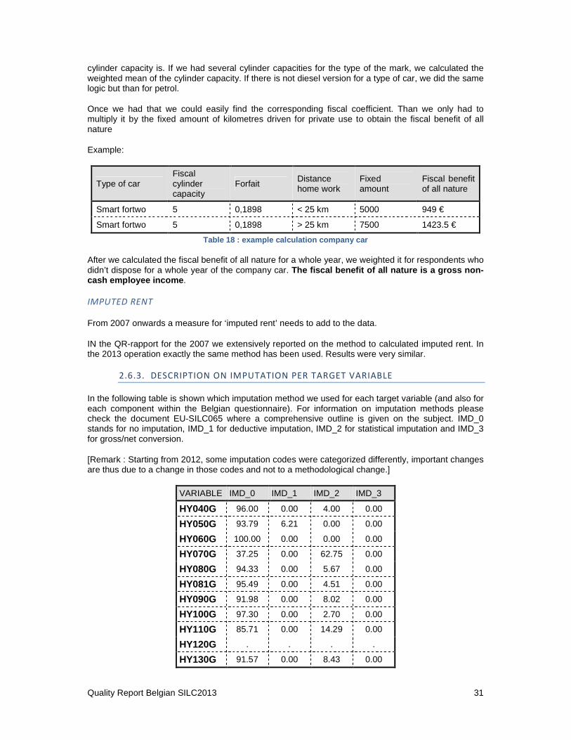
Quality Report Belgian SILC2013 31
cylinder capacity is. If we had several cylinder capacities for the type of the mark, we calculated the weighted mean of the cylinder capacity. If there is not diesel version for a type of car, we did the same logic but than for petrol.
Once we had that we could easily find the corresponding fiscal coefficient. Than we only had to multiply it by the fixed amount of kilometres driven for private use to obtain the fiscal benefit of all nature
Example:
Type of car Fiscal cylinder capacity
Forfait Distance home work
Fixed amount
Fiscal benefit of all nature
Smart fortwo 5 0,1898 < 25 km 5000 949 €
Smart fortwo 5 0,1898 > 25 km 7500 1423.5 €
Table 18 : example calculation company car
After we calculated the fiscal benefit of all nature for a whole year, we weighted it for respondents who didn’t dispose for a whole year of the company car. The fiscal benefit of all nature is a gross non-cash employee income .
IMPUTED RENT
From 2007 onwards a measure for ‘imputed rent’ needs to add to the data.
IN the QR-rapport for the 2007 we extensively reported on the method to calculated imputed rent. In the 2013 operation exactly the same method has been used. Results were very similar.
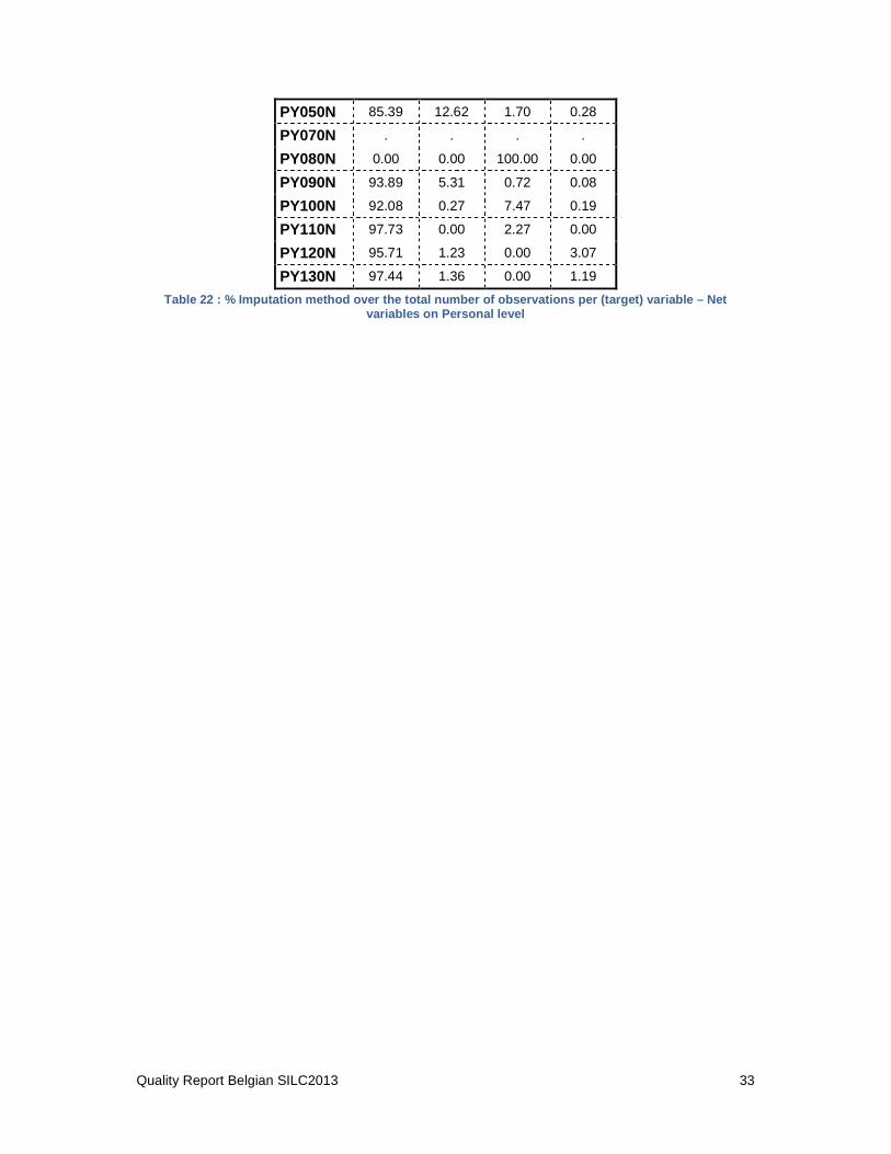
2.6.3. DESCRIPTION ON IMPUTATION PER TARGET VARIABLE
In the following table is shown which imputation method we used for each target variable (and also for each component within the Belgian questionnaire). For information on imputation methods please check the document EU-SILC065 where a comprehensive outline is given on the subject. IMD_0 stands for no imputation, IMD_1 for deductive imputation, IMD_2 for statistical imputation and IMD_3 for gross/net conversion.
[Remark : Starting from 2012, some imputation codes were categorized differently, important changes are thus due to a change in those codes and not to a methodological change.]
VARIABLE IMD_0 IMD_1 IMD_2 IMD_3
HY040G 96.00 0.00 4.00 0.00
HY050G 93.79 6.21 0.00 0.00
HY060G 100.00 0.00 0.00 0.00
HY070G 37.25 0.00 62.75 0.00
HY080G 94.33 0.00 5.67 0.00
HY081G 95.49 0.00 4.51 0.00
HY090G 91.98 0.00 8.02 0.00
HY100G 97.30 0.00 2.70 0.00
HY110G 85.71 0.00 14.29 0.00
HY120G . . . .
HY130G 91.57 0.00 8.43 0.00
Quality Report Belgian SILC2013 32
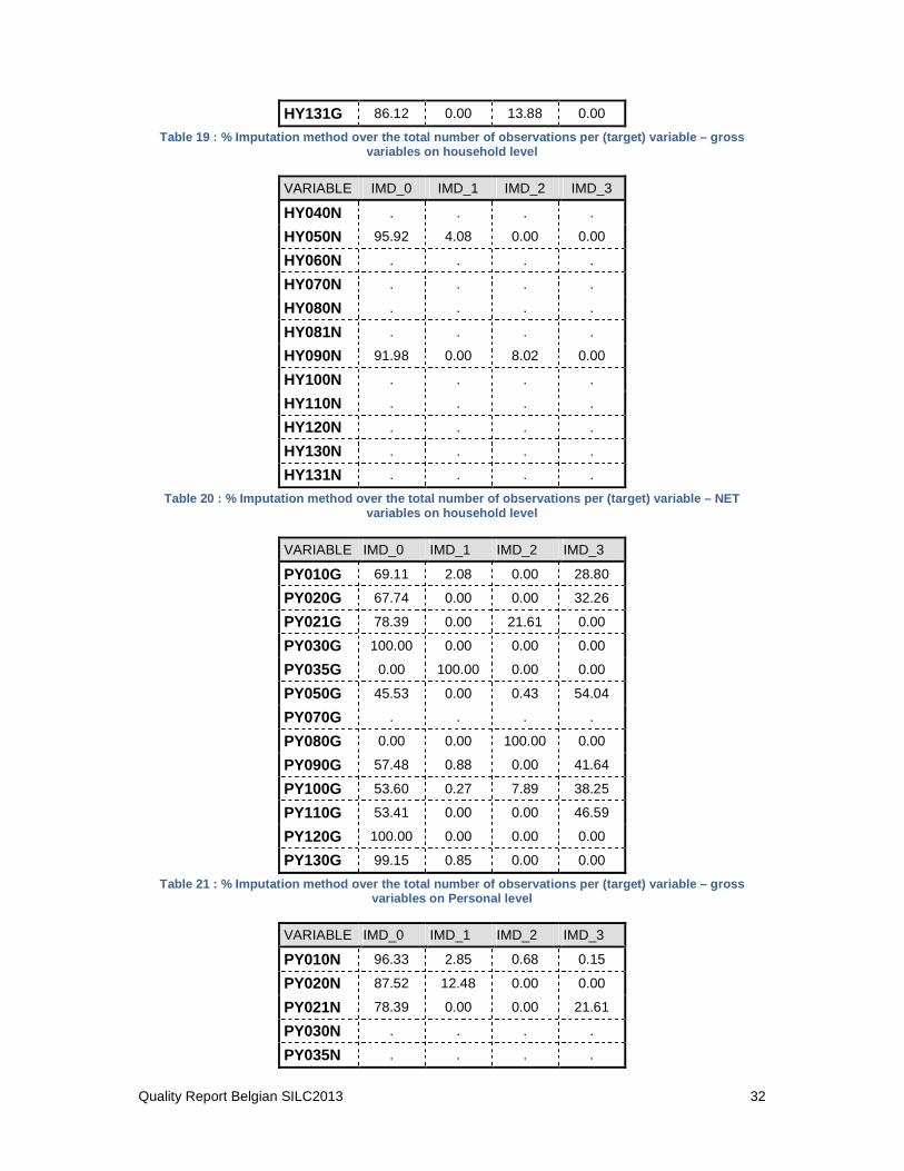
HY131G 86.12 0.00 13.88 0.00
Table 19 : % Imputation method over the total numbe r of observations per (target) variable – gross variables on household level
VARIABLE IMD_0 IMD_1 IMD_2 IMD_3
HY040N . . . .
HY050N 95.92 4.08 0.00 0.00
HY060N . . . .
HY070N . . . .
HY080N . . . .
HY081N . . . .
HY090N 91.98 0.00 8.02 0.00
HY100N . . . .
HY110N . . . .
HY120N . . . .
HY130N . . . .
HY131N . . . .
Table 20 : % Imputation method over the total numbe r of observations per (target) variable – NET variables on household level
VARIABLE IMD_0 IMD_1 IMD_2 IMD_3
PY010G 69.11 2.08 0.00 28.80
PY020G 67.74 0.00 0.00 32.26
PY021G 78.39 0.00 21.61 0.00
PY030G 100.00 0.00 0.00 0.00
PY035G 0.00 100.00 0.00 0.00
PY050G 45.53 0.00 0.43 54.04
PY070G . . . .
PY080G 0.00 0.00 100.00 0.00
PY090G 57.48 0.88 0.00 41.64
PY100G 53.60 0.27 7.89 38.25
PY110G 53.41 0.00 0.00 46.59
PY120G 100.00 0.00 0.00 0.00
PY130G 99.15 0.85 0.00 0.00
Table 21 : % Imputation method over the total numbe r of observations per (target) variable – gross variables on Personal level
VARIABLE IMD_0 IMD_1 IMD_2 IMD_3
PY010N 96.33 2.85 0.68 0.15
PY020N 87.52 12.48 0.00 0.00
PY021N 78.39 0.00 0.00 21.61
PY030N . . . .
PY035N . . . .
Quality Report Belgian SILC2013 33
PY050N 85.39 12.62 1.70 0.28
PY070N . . . .
PY080N 0.00 0.00 100.00 0.00
PY090N 93.89 5.31 0.72 0.08
PY100N 92.08 0.27 7.47 0.19
PY110N 97.73 0.00 2.27 0.00
PY120N 95.71 1.23 0.00 3.07
PY130N 97.44 1.36 0.00 1.19
Table 22 : % Imputation method over the total numbe r of observations per (target) variable – Net variables on Personal level
Quality Report Belgian SILC2013 34
3. COMPARABILITY
3.1. BASIC CONCEPTS AND DEFINITIONS
THE REFERENCE POPULATION
The reference population is all citizens living officially living at Belgian territory (population de jure). This means that the source of our sample is the central population register. This Register includes all private households and their current members residing in the territory. Persons living in collective households and in institutions are excluded from the target population.
(see also §2.3.1)
THE PRIVATE HOUSEHOLD DEFINITION
The definition of household that Eurostat recommends is used. Household is defined as a person living alone or a group of people who live together in the same dwelling and share expenditures including the joint provision of the essentials of living.
THE HOUSEHOLD MEMBERSHIP
The definition of household membership is the same as mentioned in the Eurostat document EU-SILC065/03 about the description of target variables (Chapter ‘Units’).
All household members of 16 year and older at the end of the income reference period , are selected for a personal interview.
THE INCOME REFERENCE PERIOD USED
The income reference period is a fixed twelve-month period, namely the previous calendar year. For SILC 2013, the income reference period is the year 2012.
THE PERIOD FOR TAXES ON INCOME AND SOCIAL INSURANCE CONTRIBUTIONS
This is also fixed twelve-month period, namely the previous calendar year. For SILC 2013, the period is the year 2012.
THE LAG BETWEEN THE INCOME REFERENCE PERIOD AND CURRENT VARIABLES
The income reference period is the previous calendar year (year 2012) and the current variables refer to the fieldwork period (April-December 2013). Therefore the lag is at minimum 4 months and at maximum 12 months.
THE TOTAL DURATION OF THE DATA COLLECTION OF THE SAMPLE
The fieldwork took mainly place from February to August 2013. Some interviews also took place after August 2013, they represent less than 15 % of the interviews.
Frequency Percent Cumulative Percent
January 1 0.02 0.02
February 2 0.03 0.05
March 8 0.13 0.18
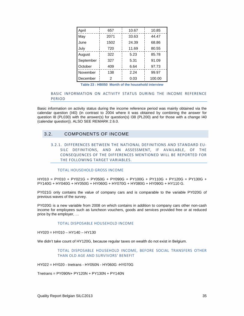
Quality Report Belgian SILC2013 35
April 657 10.67 10.85
May 2071 33.63 44.47
June 1502 24.39 68.86
July 720 11.69 80.55
August 322 5.23 85.78
September 327 5.31 91.09
October 409 6.64 97.73
November 138 2.24 99.97
December 2 0.03 100.00
Table 23 : HB050 Month of the household interview
BASIC INFORMATION ON ACTIVITY STATUS DURING THE INCOME REFERENCE
PERIOD
Basic information on activity status during the income reference period was mainly obtained via the calendar question (I40) (in contrast to 2004 where it was obtained by combining the answer for question I8 (PL030) with the answer(s) for question(s) I38 (PL200) and for those with a change I40 (calendar question)). ALSO SEE REMARK 2.6.0.
3.2. COMPONENTS OF INCOME
3.2.1. DIFFERENCES BETWEEN THE NATIONAL DEFINITIONS AND STANDARD EU-
SILC DEFINITIONS, AND AN ASSESSMENT, IF AVAILABLE, OF THE
CONSEQUENCES OF THE DIFFERENCES MENTIONED WILL BE REPORTED FOR
THE FOLLOWING TARGET VARIABLES.
TOTAL HOUSEHOLD GROSS INCOME
HY010 = PY010 + PY021G + PY050G + PY090G + PY100G + PY110G + PY120G + PY130G + PY140G + HY040G + HY050G + HY060G + HY070G + HY080G + HY090G + HY110 G.
PY021G only contains the value of company cars and is comparable to the variable PY020G of previous waves of the survey.
PY020G is a new variable from 2008 on which contains in addition to company cars other non-cash income for employees such as luncheon vouchers, goods and services provided free or at reduced price by the employer, …
TOTAL DISPOSABLE HOUSEHOLD INCOME
HY020 = HY010 – HY140 – HY130
We didn’t take count of HY120G, because regular taxes on wealth do not exist in Belgium.
TOTAL DISPOSABLE HOUSEHOLD INCOME, BEFORE SOCIAL TRANSFERS OTHER
THAN OLD AGE AND SURVIVORS’ BENEFIT
HY022 = HY020 - tnetrans - HY050N - HY060G -HY070G
Tnetrans = PY090N+ PY120N + PY130N + PY140N
Quality Report Belgian SILC2013 36
TOTAL DISPOSABLE HOUSEHOLD INCOME, BEFORE SOCIAL TRANSFERS
INCLUDING OLD AGE AND SURVIVORS’ BENEFIT
HY023 = HY020 - tnetran2 - HY050N - HY060G -HY070G.
tnetran2 = PY090N+ PY120N + PY130N + PY140G + PY100N + PY110N.
IMPUTED RENT
For more information on how imputed rent was implemented in the Belgian EU-SILC – see QR2008
INCOME FROM RENTAL OF PROPERTY OR LAND
Asked as Eurostat recommends. Income from rental of a property or land refers to the income received, during the income reference period, from renting a property (for example renting a dwelling –not included in the profit/loss of unincorporated enterprises-, receipts from boarders or lodgers, or rent from land) after deducting costs such as mortgage interest repayments, minor repairs, maintenance, insurance and other charges.
FAMILY/CHILDREN RELATED ALLOWANCES
Family / children related allowance includes:
Income maintenance benefit in the event of childbirth
Birth grant
Parental leave benefit
Family or child allowance.
From SILC 2008 onwards Belgium asked allowances received from the federal government and also birth grants given by some local authorities and medical organizations.
SOCIAL EXCLUSION PAYMENTS NOT ELSEWHERE CLASSIFIED
Social benefits in the function ‘social exclusion not elsewhere classified’ includes for Belgium:
Income support: periodic payments to people with insufficient resources.
Other cash benefit: support for destitute and vulnerable persons to help alleviate poverty or assist in difficult situations.
Belgium only took into account the Benefits paid by the Public Social Welfare Organization (not the benefits paid by private or non profit organizations).
HOUSING ALLOWANCES
The housing allowances for Belgium includes: - Rent benefit - Benefit to owner–occupiers: a means-tested transfer by a public authority to owner-occupiers
to alleviate their current housing costs: in practice help with paying mortgages and/ or interest
It excludes: • Social housing policy organized through the fiscal system
All capital transfers (in particular investment grants), for example rehabilitation subsidy and/or a building subsidy.

Quality Report Belgian SILC2013 37
REGULAR INTER – HOUSEHOLD CASH TRANSFERS RECEIVED
Regular inter-household cash transfers received refer to regular monetary amounts received, during the income reference period, from other households or persons. More precise, we asked for 'alimony and child support' and 'regular cash support'.
INTEREST, DIVIDENDS, PROFIT FROM CAPITAL INVESTMENTS IN INCORPORATED
BUSINESSES
Interest, dividends, profits from capital investment in an unincorporated business refer to the amount of interest from assets such as bank accounts, certificates of deposit, bonds, etc, dividends and profits from capital investment in an unincorporated business, in which the person does not work, received during the income reference period less expenses incurred.
For this variable (HY090), the imputation method has been adapted in 2012, so the observed decrease cannot be interpreted as a real one. The impact on the main poverty indicators has been tested and the impact on those is minor.
INTEREST PAID ON MORTGAGE
Interest paid on mortgage refers to the total gross amount, before deducting any tax credit or tax allowance, of mortgage interest on the main residence of the household during income reference period.
INCOME RECEIVED BY PEOPLE AGED UNDER 16
Income received by people aged under 16 is defined as the gross income received by all household members aged under sixteen during the income reference period. We asked the reference person the annual amount received by all children under 16 together.
REGULAR TAXES ON WEALTH
This variable isn’t asked/measured for the SILC2013 in Belgium. The reason is that the regular tax on wealth doesn’t exist.
REGULAR INTER-HOUSEHOLD TRANSFERS PAID
Regular inter-household transfer paid refers to regular monetary amount paid, during the income reference period, to other households. More precise, we asked for 'alimony and child support' and 'regular cash support'.
TAX ON INCOME AND SOCIAL INSURANCE CONTRIBUTIONS
Tax on income refers to taxes on income, profits and capital gains. They are assessed on the actual or presumed income of individuals, households or tax-unit. They include taxes assessed on holdings of property, land or real estate when these holdings are used as a basis for estimating the income of their owners.
Taxes on income include the sum of the following calculations: - (Gross income from salaries – net income salaries) - + (Gross income from self-employments – net income from self-employments) - + (Gross income from pension allowances – net income from pension allowances) - + (Gross income from disability, illness allowances – net income disability, illness allowances) - + (Gross income from jobseeker’s allowances - net income from jobseeker’s allowances)
We have also taken into account of the money that people have received from the taxes or that people have paid to the taxes in 2012 (based on their incomes of the year 2011).

Quality Report Belgian SILC2013 38
REPAYMENTS/RECEIPTS FOR TAX ADJUSTMENTS
Repayments/receipts for tax adjustments refer to the money paid to/received from Taxes Authorities related to the income received. This variable is already included in the variable ‘ tax on income and social contribution’ (see above), so Belgium didn’t provide this variable.
CASH OR NEAR-CASH EMPLOYEE INCOME
It includes: - Wages and salaries paid in cash for time worked or work done in main and any secondary or
casual job(s). - Remuneration for time not worked (e.g. holiday payments) - Enhanced rates of pay for overtime - Fees paid to directors of incorporated enterprises - Commissions, tips and gratuities - Supplementary payments (e.g. thirteenth month payments, fourteenth month payments) - Profit sharing and bonuses paid in cash - Additional payments based on productivity - Allowances paid for working in remote locations (regarded as part of the conditions of the job) - Allowances for transport to or from work
NON-CASH EMPLOYEE INCOME AND COMPANY CAR.
Before SILC 2008 variable PY020 consisted only out of ‘company Car’. From 2008 onwards other non-cash income elements needed to be added. ‘Company car’ itself was recorded in PY021.
In SILC-2013 PY020 consists of the following elements: - Company car - free or subsidized meals and luncheon vouchers - reimbursement or payment of housing-related expenses - reimbursement or payment of gasoline - reimbursement or payment of car assurance - reimbursement or payment of mobile phone costs
EMPLOYERS’ SOCIAL INSURANCE CONTRIBUTION
The outcome of variable PY030 was the result of the following model:
For blue collar workers: ((PY010G*1,08)/100)*50,5
And for white collar workers: PY010G/3
Both equations were derived from social security rules.
CASH PROFITS OR LOSSES FROM SELF-EMPLOYMENT (INCLUDING ROYALTIES)
It includes: - Net operating profit or loss accruing to working owners of, or partners in, an unincorporated
enterprise, less interest on business loans. - Royalties earned on writing, inventions, and so on not included in the profit/loss of
unincorporated enterprises. - Rentals from business buildings, vehicles, equipment, etc not included in the profit/loss of
unincorporated enterprises, after deduction of related costs such as interest on associated loans, repairs and maintenance and insurance charges.
VALUE OF GOODS PRODUCED FOR OWN CONSUMPTION

Quality Report Belgian SILC2013 39
This variable is not recorded in the file because the value of goods produced for the own consumption does not constitute a significant component of the income. The importance of the component has been assessed using HBS.
UNEMPLOYMENT BENEFITS
Unemployment benefits include: - Full unemployment benefits: benefits compensating for loss of earnings - Partial unemployment benefits - Early retirement for labour market reasons - Vocational training allowance - Mobility and resettlement - Severance and termination payments - Redundancy compensation - Subsistence income for persons entering the labour market
OLD-AGE BENEFIT
Old age benefit includes: - Old age pensions - Anticipated old age pensions - Partial retirement pensions - Survivor’s benefits paid after the standard retirement age - Disability cash benefits paid after standard retirement age
SURVIVORS’ BENEFITS
It includes: - Survivor’s pension - Death grant - Other cash benefit
SICKNESS’ BENEFITS
It includes: - Paid sick leave
DISABILITY BENEFITS
It includes: - disability pension - early retirement in case of reduced ability to work - care allowance - economic integration of the handicapped - disability benefits to disabled children in their own right - other cash benefit
EDUCATION-RELATED ALLOWANCES
It includes allowances referring to grants, scholarships and other education help received by students.
However to obtain this variable we asked the information on household level instead of personal level because in Belgium this is paid on household level. Afterwards we attributed this amount to the persons in the individual file.
CAPACITY TO FACE UNEXPECTED FINANCIAL EXPENSES (HS060)
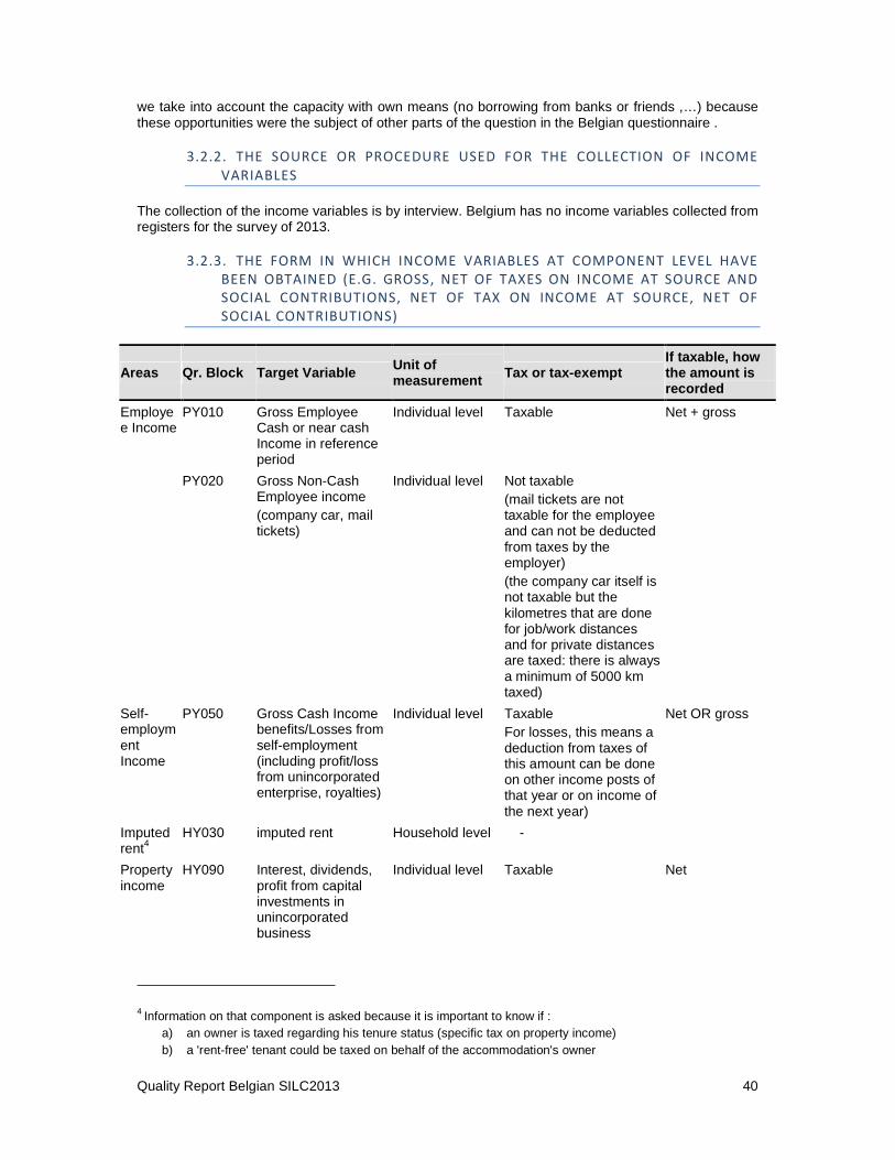
Quality Report Belgian SILC2013 40
we take into account the capacity with own means (no borrowing from banks or friends ,…) because these opportunities were the subject of other parts of the question in the Belgian questionnaire .
3.2.2. THE SOURCE OR PROCEDURE USED FOR THE COLLECTION OF INCOME
VARIABLES
The collection of the income variables is by interview. Belgium has no income variables collected from registers for the survey of 2013.
3.2.3. THE FORM IN WHICH INCOME VARIABLES AT COMPONENT LEVEL HAVE
BEEN OBTAINED (E.G. GROSS, NET OF TAXES ON INCOME AT SOURCE AND
SOCIAL CONTRIBUTIONS, NET OF TAX ON INCOME AT SOURCE, NET OF
SOCIAL CONTRIBUTIONS)
Areas Qr. Block Target Variable Unit of measurement Tax or tax-exempt
If taxable, how the amount is recorded
Employee Income
PY010 Gross Employee Cash or near cash Income in reference period
Individual level Taxable Net + gross
PY020 Gross Non-Cash Employee income (company car, mail tickets)
Individual level Not taxable (mail tickets are not taxable for the employee and can not be deducted from taxes by the employer) (the company car itself is not taxable but the kilometres that are done for job/work distances and for private distances are taxed: there is always a minimum of 5000 km taxed)
Self-employment Income
PY050 Gross Cash Income benefits/Losses from self-employment (including profit/loss from unincorporated enterprise, royalties)
Individual level Taxable For losses, this means a deduction from taxes of this amount can be done on other income posts of that year or on income of the next year)
Net OR gross
Imputed rent4
HY030 imputed rent Household level -
Property income
HY090 Interest, dividends, profit from capital investments in unincorporated business
Individual level Taxable Net
4 Information on that component is asked because it is important to know if : a) an owner is taxed regarding his tenure status (specific tax on property income) b) a 'rent-free' tenant could be taxed on behalf of the accommodation's owner
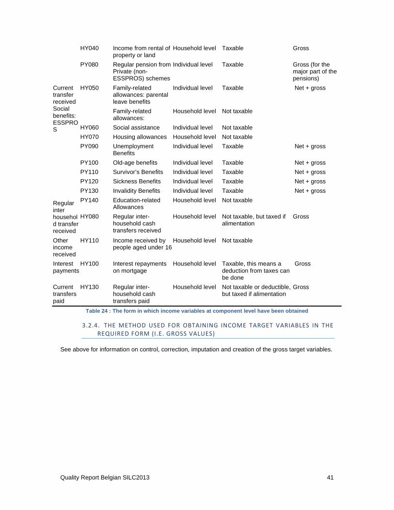
Quality Report Belgian SILC2013 41
HY040 Income from rental of property or land
Household level Taxable Gross
PY080 Regular pension from Private (non-ESSPROS) schemes
Individual level Taxable Gross (for the major part of the pensions)
Current transfer received Social benefits: ESSPROS Regular inter household transfer received
HY050 Family-related allowances: parental leave benefits
Individual level Taxable Net + gross
Family-related allowances:
Household level Not taxable
HY060 Social assistance Individual level Not taxable
HY070 Housing allowances Household level Not taxable
PY090 Unemployment Benefits
Individual level Taxable Net + gross
PY100 Old-age benefits Individual level Taxable Net + gross
PY110 Survivor’s Benefits Individual level Taxable Net + gross
PY120 Sickness Benefits Individual level Taxable Net + gross
PY130 Invalidity Benefits Individual level Taxable Net + gross
PY140 Education-related Allowances
Household level Not taxable
HY080 Regular inter-household cash transfers received
Household level Not taxable, but taxed if alimentation
Gross
Other income received
HY110 Income received by people aged under 16
Household level Not taxable
Interest payments
HY100 Interest repayments on mortgage
Household level Taxable, this means a deduction from taxes can be done
Gross
Current transfers paid
HY130 Regular inter-household cash transfers paid
Household level Not taxable or deductible, but taxed if alimentation
Gross
Table 24 : The form in which income variables at co mponent level have been obtained
3.2.4. THE METHOD USED FOR OBTAINING INCOME TARGET VARIABLES IN THE
REQUIRED FORM (I.E. GROSS VALUES)
See above for information on control, correction, imputation and creation of the gross target variables.

Quality Report Belgian SILC2013 42
4. COHERENCE
The results of the Belgian EU-SILC 2013 operation are very similar to those of the 2012 operation.

Quality Report Belgian SILC2013
43
43
ANNEX: CONFIDENCE INTERVALS
Confidence intervals (95%) for the common cross-sectional EU indicators, equivalised disposable income.
Indicator Subpopulation (if any) N value CL95low CL95high Half length
Poverty rate (ALL) 14623 15.1 12.9 17.3 2.2
Poverty rate Male 7201 14.6 12.3 16.9 2.3
Poverty rate Female 7422 15.5 13.3 17.7 2.2
Poverty rate Age 0-64 12196 14.4 12.8 16.0 1.6
Poverty rate Age 16+ 11711 14.7 12.4 17.0 2.3
Poverty rate Age 16-64 9284 13.7 12.1 15.3 1.6
Poverty rate Age 0-15 2912 16.8 14.0 19.6 2.8
Poverty rate Age 16-24 1554 17.0 14.0 20.0 3.0
Poverty rate Age 25-49 4734 13.8 12.0 15.6 1.8
Poverty rate Age 50-64 2996 11.7 9.4 14.0 2.3
Poverty rate Age 65+ 2427 18.4 11.7 25.1 6.7
Poverty rate One person hh under 65 years 1149 26.4 20.7 32.1 5.7
Poverty rate One person hh over 65 years 727 21.2 11.8 30.6 9.4
Poverty rate One person hh male 867 25.2 18.6 31.8 6.6
Poverty rate One person hh female 1009 23.9 16.6 31.2 7.3
Poverty rate One person hh total 1876 24.5 18.4 30.6 6.1
Poverty rate 2 adults (no children) both less 65 years 1916 8.7 6.4 11.0 2.3
Poverty rate 2 adults (no children) at least one 65+ years 1728 16.9 11.0 22.8 5.9
Poverty rate Other households no dependent children 1024 6.0 2.7 9.3 3.3
Poverty rate Single parent hh + one or more dependant children 1079 34.2 28.3 40.1 5.9
Poverty rate 2 adults + one dependent child 1647 10.6 7.6 13.6 3.0
Poverty rate 2 adults + two dependent children 2600 7.8 5.4 10.2 2.4
Poverty rate 2 adults + three or more dependent children 1705 19.9 13.3 26.5 6.6
Poverty rate Other households with dependent children 951 11.9 6.7 17.1 5.2
Poverty rate HH without dependent children 6544 15.3 11.7 18.9 3.6
Poverty rate HH with dependent children 7982 14.9 13.0 16.8 1.9
Poverty rate Owner or rent free 10908 8.1 6.0 10.2 2.1
Poverty rate Tenant 3704 34.6 30.6 38.6 4.0
Poverty rate Employed 5618 4.4 3.2 5.6 1.2
Poverty rate Unemployed 610 46.2 39.3 53.1 6.9
Poverty rate Retired 2846 15.1 8.6 21.6 6.5
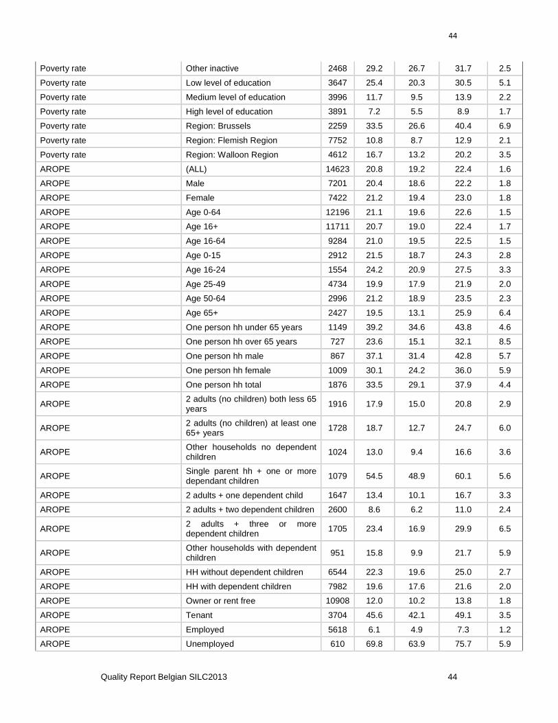
Quality Report Belgian SILC2013
44
44
Poverty rate Other inactive 2468 29.2 26.7 31.7 2.5
Poverty rate Low level of education 3647 25.4 20.3 30.5 5.1
Poverty rate Medium level of education 3996 11.7 9.5 13.9 2.2
Poverty rate High level of education 3891 7.2 5.5 8.9 1.7
Poverty rate Region: Brussels 2259 33.5 26.6 40.4 6.9
Poverty rate Region: Flemish Region 7752 10.8 8.7 12.9 2.1
Poverty rate Region: Walloon Region 4612 16.7 13.2 20.2 3.5
AROPE (ALL) 14623 20.8 19.2 22.4 1.6
AROPE Male 7201 20.4 18.6 22.2 1.8
AROPE Female 7422 21.2 19.4 23.0 1.8
AROPE Age 0-64 12196 21.1 19.6 22.6 1.5
AROPE Age 16+ 11711 20.7 19.0 22.4 1.7
AROPE Age 16-64 9284 21.0 19.5 22.5 1.5
AROPE Age 0-15 2912 21.5 18.7 24.3 2.8
AROPE Age 16-24 1554 24.2 20.9 27.5 3.3
AROPE Age 25-49 4734 19.9 17.9 21.9 2.0
AROPE Age 50-64 2996 21.2 18.9 23.5 2.3
AROPE Age 65+ 2427 19.5 13.1 25.9 6.4
AROPE One person hh under 65 years 1149 39.2 34.6 43.8 4.6
AROPE One person hh over 65 years 727 23.6 15.1 32.1 8.5
AROPE One person hh male 867 37.1 31.4 42.8 5.7
AROPE One person hh female 1009 30.1 24.2 36.0 5.9
AROPE One person hh total 1876 33.5 29.1 37.9 4.4
AROPE 2 adults (no children) both less 65 years 1916 17.9 15.0 20.8 2.9
AROPE 2 adults (no children) at least one 65+ years 1728 18.7 12.7 24.7 6.0
AROPE Other households no dependent children 1024 13.0 9.4 16.6 3.6
AROPE Single parent hh + one or more dependant children 1079 54.5 48.9 60.1 5.6
AROPE 2 adults + one dependent child 1647 13.4 10.1 16.7 3.3
AROPE 2 adults + two dependent children 2600 8.6 6.2 11.0 2.4
AROPE 2 adults + three or more dependent children 1705 23.4 16.9 29.9 6.5
AROPE Other households with dependent children 951 15.8 9.9 21.7 5.9
AROPE HH without dependent children 6544 22.3 19.6 25.0 2.7
AROPE HH with dependent children 7982 19.6 17.6 21.6 2.0
AROPE Owner or rent free 10908 12.0 10.2 13.8 1.8
AROPE Tenant 3704 45.6 42.1 49.1 3.5
AROPE Employed 5618 6.1 4.9 7.3 1.2
AROPE Unemployed 610 69.8 63.9 75.7 5.9
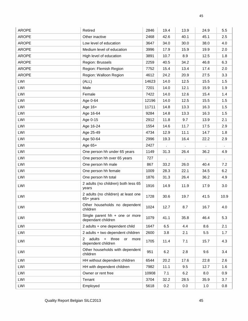
Quality Report Belgian SILC2013
45
45
AROPE Retired 2846 19.4 13.9 24.9 5.5
AROPE Other inactive 2468 42.6 40.1 45.1 2.5
AROPE Low level of education 3647 34.0 30.0 38.0 4.0
AROPE Medium level of education 3996 17.9 15.9 19.9 2.0
AROPE High level of education 3891 10.7 8.9 12.5 1.8
AROPE Region: Brussels 2259 40.5 34.2 46.8 6.3
AROPE Region: Flemish Region 7752 15.4 13.4 17.4 2.0
AROPE Region: Walloon Region 4612 24.2 20.9 27.5 3.3
LWI (ALL) 14623 14.0 12.5 15.5 1.5
LWI Male 7201 14.0 12.1 15.9 1.9
LWI Female 7422 14.0 12.6 15.4 1.4
LWI Age 0-64 12196 14.0 12.5 15.5 1.5
LWI Age 16+ 11711 14.8 13.3 16.3 1.5
LWI Age 16-64 9284 14.8 13.3 16.3 1.5
LWI Age 0-15 2912 11.8 9.7 13.9 2.1
LWI Age 16-24 1554 14.6 11.7 17.5 2.9
LWI Age 25-49 4734 12.9 11.1 14.7 1.8
LWI Age 50-64 2996 19.3 16.4 22.2 2.9
LWI Age 65+ 2427 . . . .
LWI One person hh under 65 years 1149 31.3 26.4 36.2 4.9
LWI One person hh over 65 years 727 . . . .
LWI One person hh male 867 33.2 26.0 40.4 7.2
LWI One person hh female 1009 28.3 22.1 34.5 6.2
LWI One person hh total 1876 31.3 26.4 36.2 4.9
LWI 2 adults (no children) both less 65 years 1916 14.9 11.9 17.9 3.0
LWI 2 adults (no children) at least one 65+ years 1728 30.6 19.7 41.5 10.9
LWI Other households no dependent children 1024 12.7 8.7 16.7 4.0
LWI Single parent hh + one or more dependant children 1079 41.1 35.8 46.4 5.3
LWI 2 adults + one dependent child 1647 6.5 4.4 8.6 2.1
LWI 2 adults + two dependent children 2600 3.8 2.1 5.5 1.7
LWI 2 adults + three or more dependent children 1705 11.4 7.1 15.7 4.3
LWI Other households with dependent children 951 6.2 2.8 9.6 3.4
LWI HH without dependent children 6544 20.2 17.6 22.8 2.6
LWI HH with dependent children 7982 11.1 9.5 12.7 1.6
LWI Owner or rent free 10908 7.1 6.2 8.0 0.9
LWI Tenant 3704 32.2 28.5 35.9 3.7
LWI Employed 5618 0.2 0.0 1.0 0.8
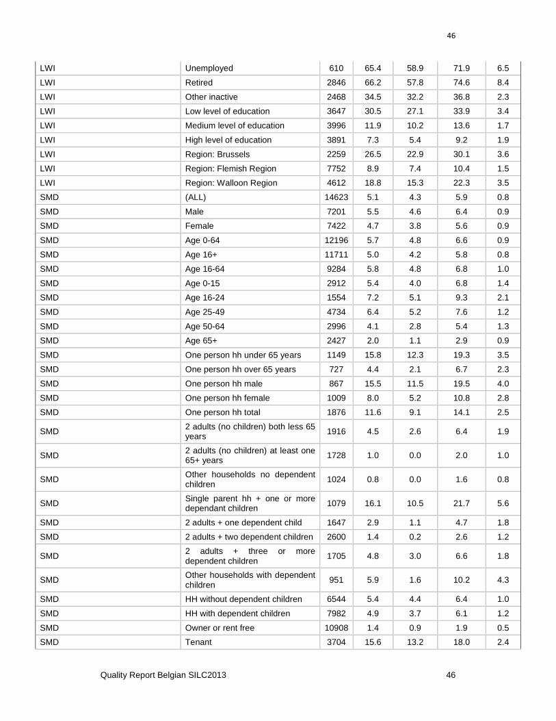
Quality Report Belgian SILC2013
46
46
LWI Unemployed 610 65.4 58.9 71.9 6.5
LWI Retired 2846 66.2 57.8 74.6 8.4
LWI Other inactive 2468 34.5 32.2 36.8 2.3
LWI Low level of education 3647 30.5 27.1 33.9 3.4
LWI Medium level of education 3996 11.9 10.2 13.6 1.7
LWI High level of education 3891 7.3 5.4 9.2 1.9
LWI Region: Brussels 2259 26.5 22.9 30.1 3.6
LWI Region: Flemish Region 7752 8.9 7.4 10.4 1.5
LWI Region: Walloon Region 4612 18.8 15.3 22.3 3.5
SMD (ALL) 14623 5.1 4.3 5.9 0.8
SMD Male 7201 5.5 4.6 6.4 0.9
SMD Female 7422 4.7 3.8 5.6 0.9
SMD Age 0-64 12196 5.7 4.8 6.6 0.9
SMD Age 16+ 11711 5.0 4.2 5.8 0.8
SMD Age 16-64 9284 5.8 4.8 6.8 1.0
SMD Age 0-15 2912 5.4 4.0 6.8 1.4
SMD Age 16-24 1554 7.2 5.1 9.3 2.1
SMD Age 25-49 4734 6.4 5.2 7.6 1.2
SMD Age 50-64 2996 4.1 2.8 5.4 1.3
SMD Age 65+ 2427 2.0 1.1 2.9 0.9
SMD One person hh under 65 years 1149 15.8 12.3 19.3 3.5
SMD One person hh over 65 years 727 4.4 2.1 6.7 2.3
SMD One person hh male 867 15.5 11.5 19.5 4.0
SMD One person hh female 1009 8.0 5.2 10.8 2.8
SMD One person hh total 1876 11.6 9.1 14.1 2.5
SMD 2 adults (no children) both less 65 years 1916 4.5 2.6 6.4 1.9
SMD 2 adults (no children) at least one 65+ years 1728 1.0 0.0 2.0 1.0
SMD Other households no dependent children 1024 0.8 0.0 1.6 0.8
SMD Single parent hh + one or more dependant children 1079 16.1 10.5 21.7 5.6
SMD 2 adults + one dependent child 1647 2.9 1.1 4.7 1.8
SMD 2 adults + two dependent children 2600 1.4 0.2 2.6 1.2
SMD 2 adults + three or more dependent children
1705 4.8 3.0 6.6 1.8
SMD Other households with dependent children
951 5.9 1.6 10.2 4.3
SMD HH without dependent children 6544 5.4 4.4 6.4 1.0
SMD HH with dependent children 7982 4.9 3.7 6.1 1.2
SMD Owner or rent free 10908 1.4 0.9 1.9 0.5
SMD Tenant 3704 15.6 13.2 18.0 2.4

Quality Report Belgian SILC2013
47
47
SMD Employed 5618 2.1 1.5 2.7 0.6
SMD Unemployed 610 23.2 18.7 27.7 4.5
SMD Retired 2846 2.2 1.5 2.9 0.7
SMD Other inactive 2468 10.2 8.8 11.6 1.4
SMD Other inactive 2468 10.2 8.8 11.6 1.4
SMD Low level of education 3647 8.5 6.8 10.2 1.7
SMD Medium level of education 3996 4.1 3.1 5.1 1.0
SMD High level of education 3891 2.6 1.7 3.5 0.9
SMD Region: Brussels 2259 14.9 11.8 18.0 3.1
SMD Region: Flemish Region 7752 2.7 1.9 3.5 0.8
SMD Region: Walloon Region 4612 6.3 4.6 8.0 1.7
Poverty rate before transfers including pensions
(ALL) 14623 26.3 23.7 28.9 2.6
Poverty rate before transfers including pensions Male 7201 26.2 24.1 28.3 2.1
Poverty rate before transfers including pensions
Female 7422 26.5 23.1 29.9 3.4
Poverty rate before transfers including pensions
Age 0-15 3092 32.1 29.0 35.2 3.1
Poverty rate before transfers including pensions Age 16+ 11711 25.1 22.3 27.9 2.8
Poverty rate before transfers including pensions Age 16-64 9284 26.0 23.8 28.2 2.2
Poverty rate before transfers including pensions
Age 65+ 2427 21.6 15.1 28.1 6.5
Poverty rate before transfers excluding pensions (ALL) 14623 42.0 40.1 43.9 1.9
Poverty rate before transfers excluding pensions Male 7201 40.0 38.2 41.8 1.8
Poverty rate before transfers excluding pensions
Female 7422 44.0 41.5 46.5 2.5
Poverty rate before transfers excluding pensions
Age 0-15 3092 32.8 29.8 35.8 3.0
Poverty rate before transfers excluding pensions Age 16+ 11711 44.2 42.3 46.1 1.9
Poverty rate before transfers excluding pensions
Age 16-64 9284 31.7 29.7 33.7 2.0
Poverty rate before transfers excluding pensions
Age 65+ 2427 92.7 91.2 94.2 1.5
AROP 40% median income (ALL) 14623 3.9 3.0 4.8 0.9
AROP 50% median income (ALL) 14623 8.3 7.0 9.6 1.3
AROP 70% median income (ALL) 14623 24.3 22.3 26.3 2.0
Mean equivalised disposable income (ALL) 14623 23279.0 22694.7 23863.3 584.3
Median equivalised disposable income (ALL) 14623 21483.0 20610.5 22355.5 872.5
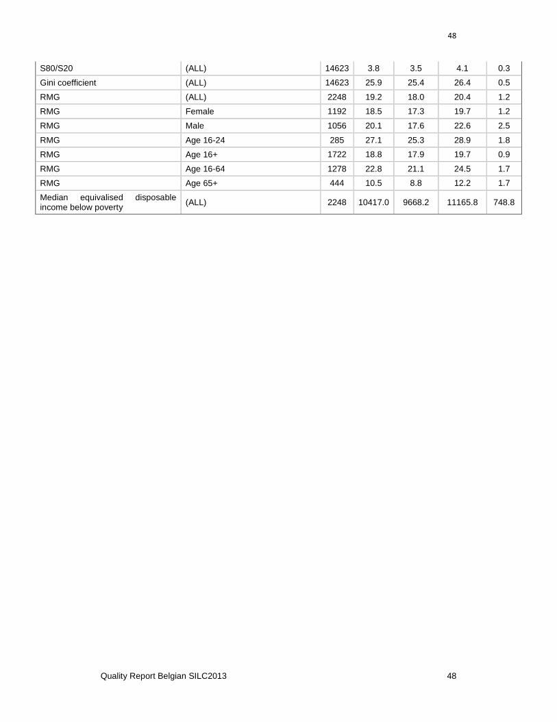
Quality Report Belgian SILC2013
48
48
S80/S20 (ALL) 14623 3.8 3.5 4.1 0.3
Gini coefficient (ALL) 14623 25.9 25.4 26.4 0.5
RMG (ALL) 2248 19.2 18.0 20.4 1.2
RMG Female 1192 18.5 17.3 19.7 1.2
RMG Male 1056 20.1 17.6 22.6 2.5
RMG Age 16-24 285 27.1 25.3 28.9 1.8
RMG Age 16+ 1722 18.8 17.9 19.7 0.9
RMG Age 16-64 1278 22.8 21.1 24.5 1.7
RMG Age 65+ 444 10.5 8.8 12.2 1.7
Median equivalised disposable income below poverty (ALL) 2248 10417.0 9668.2 11165.8 748.8