Evaluation of the register-based census

Quality assessment ofadministrative data

Documentation of Methods

STATISTICS AUSTRIA

Registers, Classifications and Methods Division

30th June 2014

Preface

The quality-framework for the assessment of administrative data was developed in coop-eration between Statistics Austria, division of register-based statistics, and Vienna Uni-versity of Economics and Business, department for economics.

This report describes the principle of the quality-assessment for administrative dataas it was used for the evaluation of the Austrian census of 2011. The detailed resultsfor 2011 can be downloaded from the Homepage of Statistics Austria.1 We would liketo thank Prof. Wilfried Grossman (University of Vienna) and Thomas Burg (StatisticsAustria) for their important contribution to the framework. Furthermore, we would liketo thank Christopher Berka, Reinhard Fiedler, Matthias Schnetzer and Christoph Waldnerfor their work in the development of the framework. Any errors that remain are in theresponsibility of the authors.

Manuela Lenk Franz AstleithnerEva-Maria Asamer Predrag Cetkovic

Henrik Rechta Stefan HumerEliane Schwerer Mathias Moser

STATISTIK AUSTRIA WU WIEN

1http://www.statistik.at/web_de/Redirect/index.htm?dDocName=076880

1

Contents

1 Introduction 3

2 Sources for the register-based census 4

3 The quality assessment of administrative data 63.1 The Raw Data Level . . . . . . . . . . . . . . . . . . . . . . . . . . . . 63.2 The Central Data Base CDB . . . . . . . . . . . . . . . . . . . . . . . . 113.3 The Final Data Pool FDP . . . . . . . . . . . . . . . . . . . . . . . . . . 12

4 Dempster-Shafer theory for the combination of evidence 144.1 Dempster-Shafer Theory . . . . . . . . . . . . . . . . . . . . . . . . . . 144.2 Application . . . . . . . . . . . . . . . . . . . . . . . . . . . . . . . . . 184.3 Artificial example for the combination of evidence . . . . . . . . . . . . 20

5 Quality assessment of imputations 225.1 Imputation process and estimating order . . . . . . . . . . . . . . . . . . 225.2 Applied imputation methods . . . . . . . . . . . . . . . . . . . . . . . . 245.3 Quality assessment of imputation models . . . . . . . . . . . . . . . . . 26

6 Conclusion 29

References 30

A Translations 33

2

Chapter 1

Introduction

The importance of administrative data as input for statistical purposes has increased steadilyin the last decades. Following the Scandinavian countries, about one third of the UnitedNations Economic Commission for Europe (UNECE) members now base their census atleast partially on administrative data (UNECE, 2014). In Austria, the last survey-basedcensus in 2001 was replaced by the first register-based census in 2011. The advantages ofthis new approach comprise inter alia reduced burden for the respondents and lower costs.However, new challenges like the assessment of the data quality arise. For this reason, var-ious books and articles were published in the last decade. Departing from Pipino, Lee, andWang (2002); Batini and Scannapieco (2006); Karr, Sanil, and Banks (2006) who have abroad understanding of data-quality, Wallgren and Wallgren (2007) developed a guidelinefor the assessment of the different dimensions of data-quality. The Scandinavian coun-tries have a long tradition in the use of administrative data (UNECE, 2007; Zhang, 2011;P. J. Daas, Ossen, Tennekes, & Nordholt, 2012; Hendriks, 2012; Axelson, Holmberg,Jansson, Werner, & Westling, 2012; Zhang, 2012). Based on this experience, StatisticsAustria developed a standardized quality framework for the assessment of administrativedata.

This report describes the conception of the quality-framework of administrative data,as it was developed and applied for the register based census of 2011. In every stageof the data processing a quality-indicator is derived for each attribute. Even though theframework was developed around the register-based census, it was designed for generalapplicability. Due to the modular design, every step of the quality-framework can beapplied individually. In the chapter 2, we will introduce the sources of the register basedcensus. In chapter 3, the quality framework is explained using the example from thequality assessment for the Legal Marital Status LMS. If an attribute is obtained frommultiple register, the information from the data sources have to combined. Chapter 4focuses on the application of Dempster-Shafer-Theory for this purpose. In chapter 5 thequality assessment of imputation is explained in detail.

3

Chapter 2

Sources for the register-based census

A decisive quality–related topic for register–based statistics is the selection of appropriatedata sources for the supply with required information.

Housing Registerof buildingsand dwellings

Central SocialSecurity Register

Register ofEducationalAttainment

Central Popu-lation Register

Tax RegisterUnemployment

Register

Business Registerof enterprises andtheir local units

+ 8 Comparison Registers

Analysis ofresidence

FamilyEducationDemography CommuterStatus of

employment

LocalUnits of

enterprises

Buildingsand

dwellings

Census of LocalUnits of enterprises

Census of PeopleCensus of Buildings

and dwellings

Figure 2.1: Data sources for the register–based census

Figure 2.1 illustrates the connections between the data sources and topics of the cen-sus. Statistics Austria distinguishes between seven base registers and eight comparisonregisters. The base registers contain, in principle, the attributes of interest for the register-based census. The red shaded registers form the backbones of the census. They determinethe population number, the number of buildings and dwellings and the number of enter-prises and their local units. To improve the quality of the results, the base registers arebacked up by eight comparison registers which gather information from more than 50 data

4

holders. They are mainly used for cross-checks and validation.1 If there is more than onesource for an attribute, the registers serve as instruments for cross-checks and validationbecause of the autonomous data delivery. This principle of redundancy helps to improvequality of data (Lenk, 2008, p. 3).

1If data is not or only partly available in the base registers, information is derived from the comparisonregisters as well (Berka et al., 2010, p. 300).

5

Chapter 3

The quality assessment ofadministrative data

Statistik Austria is not responsible for the data maintenance of the external data sourceswhich contribute the majority of the required information. Hence, the relevance of qualityassessment in the process of register–based statistics has to be emphasized. Our approachfor the assessment of administrative data was inspired by work from other National Sta-tistical Institutes NSI (P. Daas, Ossen, Vis-Visschers, & Arends-Tóth, 2009; P. Daas &Fonville, 2007) and relies on four quality-related hyperdimensions (Berka et al., 2010,2012).

The data processing for the Austrian census is divided in three levels that have to beconsidered in the quality assessment: the raw data (i.e. the registers i), the combineddataset (Central Database CDB) and the imputed dataset (Final Data Pool FDP). Fourhyperdimensions (HDD, HDP , HDE , HDI) aim to assess the quality for different typesof attributes at all stages of the data processing. Figure 3.1 illustrates the data processing,beginning with the delivery of raw data from the various administrative data holders.The data is connected via a unique personal key (branch-specific personal identificationnumber bPIN) and merged to data cubes in the CDB. Finally, missing values in the CDBare imputed in the FDP where every attribute j for every statistical unit n in the statisticsof administrative data obtains a quality indicator qnΩj . In the following, we will explainthe quality framework using the example of the calculation of the quality measure for theLegal marital Status LMS.

3.1 The Raw Data Level

We start our considerations on the quality assessment at the first level of the framework.Information on quality at the raw data level ( registers i; see blue boxes in Figure 3.1) isobtained via three hyperdimensions: Documentation (HDD), Pre-processing (HDP ) and

6

Raw

Reg 1

Aq1A

Bq1B

Cq1C

HDD HDP HDE

HDD HDP HDE

HDD HDP HDE

Reg 2

A q2A

D q2D

E q2E

HDD HDP HDE

HDD HDP HDE

HDD HDP HDE

Combined

Central Database Ψ

Aq⊙A

qΨA

Cq⊙C

qΨC

Fq⊙F

qΨF

Gq⊙GqΨG

HDE

HDE

HDE

Final

Final Data Pool Ω

AqΩA

CqΩC

FqΩF

GqΩG

HDE

HDI

qijA

HDD

HDP

HDE

HDI

Quality IndicatorAttributeMultiple AttributesUnique AttributeDerived AttributeDocumentationPre–processingExternal SourcesImputations

Abbildung 1: Quality Assessment of the Final Data PoolFigure 3.1: Quality framework for register–based censuses

External Source (HDE). The derivation of the quality measures for the Legal MaritalStatus LMS on the raw-data level can be retraced in the following tables.

Hyperdimension HDD

HDD describes quality-related processes as well as the documentation of the data (meta-data) at the administrative authorities. The degrees of confidence and reliability of the dataholders are monitored by the use of a questionnaire containing several open and scoredquestions. The open questions gather information of general interest, like the timelinessof data delivery or on the definition of the sample. This information is important for thedocumentation of the delivery but is not used for the quality assessment of the census.Table 3.1 shows the scored questions and the corresponding weights as they were usedfor the quality-assessment of the Austrian census of 2011.

Data for the LMS are obtained in eleven source registers i which have to be assessed.1

The calculation of the hyperdimension documentation HDD for each source register is il-lustrated in table 3.2. The data holders answer quality related questions on a dichotomous(Yes or No) or ordinal scale. The higher the value for each question the better should

1Source registers: ASR: Asylum Seekers Register, UR: Unemployment Register, RPS: Register of PublicServants of the Federal State and the Länder, CAR: Child Allowance Register, CFR: Central ForeignerRegister, CSSR: Central Social Security Register, CHR: Chambers Register, HPSR: Hospital for PublicServants Register, SWR: Register of Social Welfare Recipients, CPR: Central Population Register, TR: TaxRegister.

7

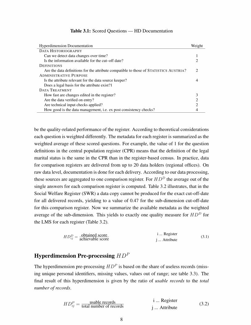
Table 3.1: Scored Questions — HD Documentation

Hyperdimension Documentation WeightDATA HISTORIOGRAPHY

Can we detect data changes over time? 1Is the information available for the cut–off date? 2

DEFINITIONSAre the data definitions for the attribute compatible to those of STATISTICS AUSTRIA? 2

ADMINISTRATIVE PURPOSEIs the attribute relevant for the data source keeper? 4Does a legal basis for the attribute exist?1

DATA TREATMENTHow fast are changes edited in the register? 3Are the data verified on entry? 2Are technical input checks applied? 2How good is the data management, i.e. ex post consistency checks? 4

be the quality-related performance of the register. According to theoretical considerationseach question is weighted differently. The metadata for each register is summarized as theweighted average of these scored questions. For example, the value of 1 for the questiondefinitions in the central population register (CPR) means that the definition of the legalmarital status is the same in the CPR than in the register-based census. In practice, datafor comparison registers are delivered from up to 20 data holders (regional offices). Onraw data level, documentation is done for each delivery. According to our data processing,these sources are aggregated to one comparison register. For HDD the average out of thesingle answers for each comparison register is computed. Table 3.2 illustrates, that in theSocial Welfare Register (SWR) a data copy cannot be produced for the exact cut-off-datefor all delivered records, yielding to a value of 0.47 for the sub-dimension cut-off-datefor this comparison register. Now we summarize the available metadata as the weightedaverage of the sub-dimension. This yields to exactly one quality measure for HDD forthe LMS for each register (Table 3.2).

HDDij = obtained score

achievable scorei ... Register

j ... Attribute(3.1)

Hyperdimension Pre-processing HDP

The hyperdimension pre-processing HDP is based on the share of useless records (miss-ing unique personal identifiers, missing values, values out of range; see table 3.3). Thefinal result of this hyperdimension is given by the ratio of usable records to the totalnumber of records.

HDPij = usable records

total number of recordsi ... Register

j ... Attribute(3.2)

8

Table 3.2: Calculation of the hyperdimension documentation HDD for the legal maritalstatus (LMS)

HD Weight ASR UR RPS CAR CFR CSSR CHR HPSR SWR CPR TR

Detect Changes 1 0 1 0.87 1 0 1 0.67 0.35 0.51 1 1Cut-off date 2 0 1 0.87 1 0 1 0.67 0.35 0.47 1 1Definitions 2 1 1 1 1 1 1 1 1 1 1 1Relevance 4 0 0 0.62 1 0 1 0.67 0.7 0.83 0 1Legal basis 1 0 1 1 1 0 1 0.67 0.35 1 1 1Timeliness 3 1 1 0.80 1 1 1 1 0.81 0.85 1 1Administrative Contr 2 0.33 0.67 0.73 1 0.33 1 0.67 0.73 0.81 1 1Technical Contr 2 0.67 0 0.70 1 0.67 1 0.78 0.49 0.77 1 1Data management 4 0.33 1 0.63 0.67 0.33 0.67 0.78 0.59 0.64 1 1

HDD 0.397 0.683 0.864 0.936 0.397 0.936 0.778 0.706 0.746 0.810 1

Table 3.3: HD Pre–processing

Number of observations— Records without unique personal identifiers— Records with item non–response (but including unique IDs)— Records with wrong values or values out of range= Usable records

The results for this hyperdimension for the LMS in the source registers are shown intable 3.4. Most data sources provided formally correct information on the LMS. How-ever, data from the Asylum Seekers Register (ASR) and Social Welfare Register (SWR)have a significant amount of missing unique personal identifiers (56.1% and 14.4%, resp.)lowering the quality indicator.

Table 3.4: Calculation of the hyperdimension HDP for the legal marital status (LMS)

Register Observations Missing bPIN % Non resp. & Out of range % HDP

ASR 66,411 56.12 3.73 0.402UR 327,702 1.30 7.74 0.910RPS 640,155 1.66 2.85 0.955CAR 3,658,263 2.72 0.01 0.973CFR 747,688 7.67 2.58 0.898

CSSR 8,811,838 6.30 48.30 0.454CHR 23,904 3.40 41.51 0.551HPSR 87,954 6.23 38.60 0.552SWR 263,134 14.44 7.24 0.783CPR 9,605,679 0.0 33.04 0.670TR 9,359,027 6.28 9.31 0.844

Hyperdimension External Source HDE

The last hyperdimension (HDE) on raw-data level assesses the data-quality of the sourceregisters in comparison to an external source, in our case, the Austrian microcensus. Itis calculated as the number of consistent values divided by the number of all records that

9

could be linked to the microcensus. If the attribute is not covered by the microcensus oranother suitable survey, an expert on the specific dataset is asked to assess the validity ofthe data on a scale between zero and one.

HDEij = number of consistent values

total number of linked recordsi ... Register

j ... Attribute(3.3)

Table 3.5: Calculation of the hyperdimension HDE for the legal marital status (LMS)

Register Linked observations Conflicting observations % HDE

ASR 10 50.0 0.500UR 1,239 1.9 0.981RPS 2,993 4.1 0.959CAR 13,905 3.0 0.970CFR 2,235 11.5 0.885

CSSR 20,346 5.8 0.942CHR 71 11.3 0.887HPSR 194 2.6 0.974SWR 576 5.2 0.948CPR 27,959 2.9 0.971TR 24,332 8.9 0.910

In table 3.5, we see the results of the comparison to an external source for the LMS.For example, 1,239 individuals from the Unemployment Register could be linked to themicrocensus. Out of these observations, 1.9 per cent were classified wrong. This yieldsto a HDE value of 0.981 for the LMS in the UR.

Final quality on the raw-data level

Given these three quality measures, an overall quality indicator for each attribute onregister-level can be derived as a weighted average. In our framework, each hyperdi-mension has the same weight (vD = vP = vE), and therefore an equal impact on thequality measure. The resulting value summarizes the existing quality-related informationfor each attribute j in each register i. Hence, this indicator is able to capture quality-related effects from the data generation through to the raw data in the registers.

qij = vD ·HDDij + vP ·HDP

ij + vE ·HDEij =

∑k∈D,P,E vk · hdkij

i ... Register, j ...Attribute(3.4)

Table 3.6 summarizes the information for the attribute LMS for each register. Hence,we obtained eleven quality indicators. ASR has the lowest quality-measure, while CARdelivers the best quality for the LMS. The quality differs partly because of the differentsubgroups covered by the registers (families with young children vs. foreign people), butalso because the LMS is relevant for the CAR but it is not for the ASR. In the next step

10

this information on data quality in the registers is used to evaluate the quality of the valuechosen for the CDB.

Table 3.6: Calculation of the quality indicator for the (LMS) for the registers

Register HDD HDP HDE q

ASR 0.397 0.402 0.500 0.433UR 0.683 0.910 0.981 0.858RPS 0.864 0.955 0.959 0.926CAR 0.936 0.973 0.970 0.960CFR 0.397 0.898 0.885 0.726

CSSR 0.936 0.454 0.942 0.777CHR 0.778 0.551 0.887 0.739HPSR 0.706 0.552 0.974 0.744SWR 0.746 0.783 0.948 0.826CPR 0.810 0.670 0.971 0.817TR 1.000 0.844 0.910 0.918

3.2 The Central Data Base CDB

The entire information from the registers is combined in the Central Database (CDB,green box in Figure 3.1) which covers all attributes of interest for the register–based cen-sus. At this level, a quality indicator qnj for each attribute j for each statistical unit n iscomputed for the first time. Concerning the evaluation of quality for the CDB we distin-guish three types of attributes by their origin.2

Unique attributes exist in exactly one register, e.g. educational attainment (cf. at-tribute C in figure 3.1). For this reason, the measure of quality in the CDB is the same asin the raw data.

Derived attributes are based on different attributes, e.g. current activity status (cf.attributes F and G in figure 3.1). The registers do not contain any information for theseattributes in the required specification, but related information.

Multiple attributes show up in several registers, e.g. LMS (cf. attribute A in figure3.1). Since there are multiple data sources providing a certain attribute, a predefinedruleset, based on experience of Statistik Austria, picks the most appropriate value fromthe underlying registers according to the constellation in the source registers. To assessthe validity of this chosen value, all the available information is taken into account. TheDempster-Shafer Theory (DST) for the combination of evidence (Chapter 4) is applied toderive a quality measure for these attributes for each statistical unit.

Depending on the type of the assessed attribute an additional comparison to an externalsource is carried out in this step.Multiple attributes, attributes that couldn’t be compared

2A detailed description of the quality assessment for the three types of attributes in the CDB is given byBerka et al. (2010, 2012).

11

to an external source on the raw-data level and attributes that are derived on CDB-levelare compared to an external source at this stage.

If we focus on our example, the LMS, the quality measures on the raw data level areconsidered as beliefs in the correctness of the value. DST for the combination of evidencetakes into account all available evidence from the registers to form one quality-indicatoron the CDB-level qn for each statistical unit n. In the next step, the values in the CDBare compared to an external source HDE .3 This yields to the last quality indicator inthe CDB qnΨ. Table 3.7 shows the last quality measures on CDB-level qnΨ, which is theweighted average of qn (Weight=0.75) and HDE (Weight=0.25). In our example qnΨ is0.728. Hence, HDE slightly increases the quality indicator.

Table 3.7: The quality for the LMS on CDB level

qn HDE qnΨ

q 0.721 0.973 0.728

3.3 The Final Data Pool FDP

In the last step of the data generation missing values in the CDB are imputed in theFDP. For the assement of the data quality in the FDP the fourth Hyperdimension HDI

is computed. For that, the distinction of methods is crucial (see Kausl, 2012). In theAustrian census deterministic editing, Hot-Deck techniques and logistic regressions areapplied. However, the principle for the evaluation of the imputations is the same for allmethods. It is based on the quality of the inputs and the quality of the imputation model.The quality of the input is assessed as a weighted average of the quality of the inputvariables, that are used for each statistical unit n.

HDIn = Φm · 1

N

N∑j=1

qΩj︸ ︷︷ ︸qInput

I ... Imputation, n ... Statistical unit, N ... Number of Inputs for m,m ... Imputation method, Φm ... Classification rate for m

(3.5)

The accuracy of the imputation models m is assessed using classification rates Φ. Theclassification rate is the number of correct imputed values, if the model is applied to exist-ing data.4 Finally, the quality of the imputations is the product of the quality of the input

3This additional comparison to an external source is only carried out for multiple and derived attributes.If an attribute is derived in the FDP, the additional external source is carried out in the FDP

4For ordinal variables the distance between the true value and the estimated value is taken into account.For numerical variables, the accuracy of the model is simply the correlation coefficient between the trueand the imputed values.

12

qInput and the accuracy of the output of the model Φm. For a detailed explanation of thequality assessment for the different imputation techniques see Chapter 5 and Astleithneret al. (forthcoming).

Table 3.8 shows the improvement of the average quality from CDB to FDP level. Theaverage quality in the CDB, where missing values have the quality of zero, for the attributeis qnΨ. Now these missing records are imputed and obtain a quality measure according totheir method of imputation. The average of the imputation quality HDI for the LMS is0.956. Formerly missing values now have a quality indicator higher than zero. For thisreason, the average quality of the LMS is higher in the FDP (qnΩ) than in the CDB (qnΨ).

Table 3.8: The quality for the LMS on FDP level

qnΨ HDI qnΩ

q 0.728 0.956 0.949

13

Chapter 4

Dempster-Shafer theory for thecombination of evidence

If attributes are obtained in multiple sources, the information on the values in the sourceregisters and their quality can be used for the assessment of the value in the CDB. Forthe combination of evidence the Dempster-Shafer theory (DST) is applied. First, we willgive an introduction to the DST. Second, we show its application for administrative data.Finally we give an artificial example for the calculation of the quality-indicator for amultiple attribute.

4.1 Dempster-Shafer Theory

Uncertainty plays an essential role in the analysis of complex systems. Nonetheless thedefinition of uncertainty in such research tasks often remains ambiguous or unclear. Usu-ally the researcher encounters uncertainty as a dual phenomenon (Helton, 1997):

Stochastic Uncertainty results from the fact that systems can behave in different ways,i.e. it is a property of the system itself.

Epistemic Uncertainty occurs due to a lack of knowledge about the system and is thusa methodological problem when performing an analysis. Accordingly epistemicuncertainty deals with the lack of knowledge about the distribution of a certainvariable itself, e.g. whether the register represents the ’true’ values.

(Hacking, 1975) traces this very important distinction between the two types of un-certainty back to the beginnings of probability theory. (Helton, 1997) states that as longas the separation between stochastic and epistemic uncertainty is not maintained care-fully, an evaluation of the systems behavior and characteristics on rational basis becomesdifficult or even impossible.

14

It is common sense that the stochastic part of uncertainty is best dealt within the so–called frequentist approach, the most important discipline of the traditional probabilitytheory. In contrast, the epistemic uncertainty is not considered carefully enough by sucha theory.

In order to deal with these shortcomings of traditional probability theory, we apply a’fuzzy approach’. Statistical fuzzy logic aims to explain epistemic uncertainty and triesto implement models for it. It can be regarded as an extension to the classical probabilitytheory and will therefore yield the same results when no uncertainty is present. Platon al-ready mentioned that besides the dual approach of either TRUE or FALSE there has to bea way to express uncertainty. Current applications of the fuzzy logic are mainly based onthe ideas of (Zadeh, 1965). He introduces fuzzy sets, in which an element can be includedor excluded, but he also allows for partial inclusion in the set. The degree of inclusionis given by a so-called membership function as a value in the interval [0,1]. These func-tions exist for each element and combined they yield the so-called fuzzy functions. Thesefunctions are generated either through statistics or opinions of experts.

To derive these ’expert opinions’, a special form of fuzzy logic can be applied. Morespecifically we use an evidence theory that was proposed by (Dempster, 1968) and ex-tended by (Shafer, 1992). This so–called Dempster–Shafer Theory focuses on a field ofprobability theory that is closely related to fuzzy logic. It allows to combine differentbeliefs about the reality, i.e. expert opinions. Eventually this results in a measure ofevidence, which can be interpreted as a probability. This approach is specifically usefulwhen an expert cannot make a definitive statement about the probability that a specificevent will occur. What he or she has is a fuzzy belief about the probability that a certainevent will arise. In this case the belief of an expert may differ from that of other experts.The Dempster-Shafer Theory aims to combine these different beliefs to come to an over-all idea of the probability, taking the uncertainty among different beliefs into account.Consider the treatment of an ill patient in a hospital. Some doctors may have differentbeliefs about the true reason for the sickness. One doctor might consider a malfunction ofthe liver as the reason and has a degree of belief of 90%. It could be that another doctorthinks of some other reasons and therefore beliefs that the malfunction of the liver is notthe main cause. An easy way to evaluate the overall belief would be a simple averagingof the different beliefs. However this approach does not consider the uncertainty nor pos-sible conflicts between expert opinions that are closely connected to the different beliefs.The Dempster–Shafer Theory tries to overcome these shortcomings by considering therole of uncertainty and conflicts within its framework.

The theory consists of three fundamental functions: the basic probability assignmentfunction (bpa), the Belief function (Bel) and the Plausibility function (Pl) (Sentz & Fer-son, 2002).

15

More formally, the power set 2X is the set of all subsets of X , including the emptyset ∅ and X itself. The elements of the power set 2X can be considered as hypothesisof the condition of a complex system. For the Census 2X can be seen as all possibleconstellations of certainty and uncertainty between registers or merely a subset of them(see table 4.3 and the explanation in the following chapter). The Dempster-Shafer Theoryof evidence assigns a specific degree of belief to each element of 2X . Formally, this isrepresented by the basic probability assignment function (bpa) (?, ?, see)]klir:1998. Thebpa defines a mapping of the power set to the interval between 0 and 1.

bpa : 2X → [0, 1]

The bpa of the empty set is 0 and the summation of the bpas of all elements of the powerset 2X equals 1.

bpa(∅) = 0∑A∈2X

bpa(A) = 1

The value of the bpa describes the proportion of evidence that encourages the hypothesisthat a particular element of X belongs to a specific element A ∈ 2X of the power set,but not a particular subset of A. It is important to note that the bpa(A) of the set A is notimply any statement about the value of the bpa for a subset of A.

Based on the basic probability assignment function we derive an interval that containsthe precise probability of the condition A of a system.

Bel(A) ≤ P (A) ≤ Pl(A)

The lower bound Belief for a certain set A is the sum of all bpas of subsets B of the setof interest A.

Bel(A) =∑

B|B⊆A

bpa(B)

The upper bound of the interval is defined as the measure of Plausibility and is evaluatedby summing up all bpas of the set B that intersect the set of interest A.

Pl(A) =∑

B|B∩A 6=∅

bpa(B)

The Beliefs (Bel) as well as the Plausibilities (Pl) do not have to sum up to 1. They arenon-additive since they are sums over an arbitrary number of subsets B out of A. Further-more, due to the fact that the basic probability assignments sum up to 1, the Plausibilitycan be derived from the measure of Belief and vice versa.

Pl(A) = 1−Bel(¬A)

16

Furthermore we can compute also bpas from e.g. give Beliefs. If Bel(A) equals Pl(A)

the probability of the condition A of a process is explicitly determined. Accordingly theDempster-Shafer Theory of Evidence yields the same results as traditional probabilitytheory. In the presence of epistemic uncertainty the values of the two measures differand form an interval of lower and upper bounds of probabilities. The actual value ofprobability is included in the interval composed of the Belief and Plausibility. Someexamples for basic probability assignment function (bpa), the Belief function (Bel) andthe Plausibility function (Pl) can be found in the Appendix.

An advantage of Dempster–Shafer’s Theory of Evidence is its capability of combin-ing information from independent sources when epistemic uncertainty is present. Gener-ally, the intention of data aggregation is to summarize and simplify information. Widelyused aggregation methods are the evaluation of averages (either in arithmetic, geometricor harmonic form) or the selection of particular properties of the data (e.g. minimum,maximum or median of an empirical distribution). Combination rules can be seen as aderivation of such rather simple aggregation techniques. Their purpose is to aggregateevidence about the condition of a system obtained from multiple data origins. Examplesfor different sources of information depend strongly on the field of application. Their rolecan be taken by a group of experts (e.g. doctors), a number of sensors (airborne radar sta-tions) or various administrative registers, which deliver information on certain attributesof statistical units of the population.

The initial rule for the combination of evidence within the Dempster–Shafer Theoryis the so–called Dempster Rule (Dempster, 1967). It can be regarded as a generalizationof Bayes’ rule and conflates multiple Belief functions by aggregating their basic proba-bility assignment functions (see equation 4.1). Dempsters Rule is a strictly conjunctiveprocedure and accents agreement of multiple sources of information.

bpa1,2(A) = (bpa1 ⊕ bpa2)(A) =1

1−K∑

B∩C=A 6=∅

bpa1(B) · bpa2(C) (4.1)

Conflicting evidence is considered through the normalisation factor 1 − K, whereas Kstands for the sum of bpas assorted with conflict, as can be seen in equation 4.2. Set-theoretic, these are all products of bpas where the intersection equals ∅.

K =∑

B∩C=∅

bpa1(B) · bpa2(C) (4.2)

This property of Dempsters Rule induced heavy criticism by (Zadeh, 1986) and (Yager,1987). As a consequence, various combination rules were proposed in the literature, likefor example Yager’s rule or Dubois and Prade’s disjunctive pooling rule. In the applicationon the quality measurement of combined administrative data sources, we disregard theirconceivable arguments because Dempsters Rule is associative (Joshi, Sahasarabudhe, &

17

Shankar, 1995). Consequently the succession of the multiple sources has no impact onthe results of our analysis. Examples for coinciding and conflicting evidence is providedin the Appendix.

4.2 Application

For the register-based census we use the Dempster-Shafer Theory to combine qualityindicators from different data sources. The quality framework aims to deliver a qualityindicator for each attribute in the Census Database (CDB), which contains informationon the population in Austria (e.g. residency, sex, status of employment). It is filled fromdifferent administrative data sources (registers) based on a predefined ruleset. The qualityindicators of the attributes in this CDB are derived based on the quality measures from theoriginal registers. If there is only one base register available to compare with, the indicatoralso resembles the quality of the CDB. In the case of multiple attributes several registershave information over the same attribute, e.g. sex may be included in four registers. Sincethese sources can be regarded as different opinions (or beliefs) on a common subject (theattribute) it allows for the implementation of the Dempster-Shafer Theory.

In a first step we assign a certain mass of certainty (C) and uncertainty (U) to each at-tribute in each register, which is based on the quality measures of these attributes qij . Thisyields 2n (n being the number of registers with the same attribute) possible combinationsof certainty and uncertainty. For the case of n = 2 that would be: CC (both certain), CUor UC (one register uncertain), UU (both registers uncertain). These different cases canbe grouped into agreement, uncertainty, logical impossibility and conflicting evidence.This process depends on the values of the attribute in the different registers, e.g. CC canbe agreement (if both registers are sure the person is ’female’) but in another case it canbe a logical impossibility (if one register is sure that the person is ’male’ and the other issure that the person is ’female’).

In some cases there are a lot of registers which contain information about the sameattribute. If the number of registers becomes large, computational difficulties will arisebecause of the assignment of the constellations of certainty and uncertainty to the cor-responding groups mentioned above. We solve them by creating (i.e. from REG1 toREGn) a look-up table for each case, which contains possible combinations of certainty(C) and uncertainty (U). In the second step we simply take the combination (e.g CCCC)from the look-up table, that corresponds to our actual case.

Note that different registers may show differing values for the same observation. Itis possible that register 1 is absolutely certain that an individual is male, while register2 is sure that this person is female (case CC), which would be a logical impossibility.Therefore it depends on the values within the different registers if CC can be regardedas agreement or logical impossibility. Accordingly it is possible to calculate different

18

Table 4.1: Table of used symbols

Symbol NameBel Degree of Beliefξ Normalisation of uncertainty Logical impossibilityω ConflictUn Uncertainty

beliefs, e.g. the belief that register 1 shows the true value or that register 2 is correct.The combination rules are calculated based on the degree of agreement, uncertainty,

logical impossibility and conflicting evidence.

Bel =1− − ω − Un

1− (4.3)

The general equations 4.3 and 4.4 are applied to each observation for each attribute.The CDB marks the actual belief for a certain observation and therefore defines whichbelief is calculated.

ξ =Un

1− (4.4)

Accordingly if an individual is male according to the CDB we check the reliability of thisinformation using the comparison registers. For each observation measures of Belief andPlausibility are constructed. These figures can be interpreted as a confidence interval forthe accuracy of each observation k. The quality indicator for each observation is nowcomputed as the mean of belief and plausibility.

qΨ,Ak=Bel(Ak) + Pl(Ak)

2

The overall quality indicator for attribute A is computed as the average over the wholepopulation.

qΨ,A =1

2n

n∑k=1

(Bel(Ak) + Pl(Ak))

We will present not only the mean for each attribute (although it is the most importantfigure for our application as it represents the quality indicator for a multiple attributewithin the CDB) but also other moments and distribution measures such as the standarddeviation or quantiles. These indicators give information on the accuracy and deviationsof our results and therefore deliver a more sophisticated picture of the quality assessmentfor an attribute in the CDB.

19

4.3 Artificial example for the combination of evidence

Table 4.2: Quality Indicators for sex in four selected registers

Register HDD HDP HDE qi,sex

REG1 0.7916 0.9424 0.9985 0.9108REG2 0.4444 0.7459 0.9966 0.7290REG3 1.0000 1.0000 0.9982 0.9994REG4 0.7916 0.9927 1.0000 0.9281

Suppose we derived the following quality indicators for the attribute sex in four regis-ters (REG1 - REG4) in the first step of the quality framework (see Table 4.2). Where thecolumns represent different quality aspects. These quality measures are combined usingweighted averages. In this case we weighted each quality aspect equally. qi,sex is thusgiven by

qi,sex =1

3HDD +

1

3HDP +

1

3HDE

There is no specific rational behind this weighting. One could apply sensitivity analy-ses to get an idea of the impact of the weights. Since in this case we can use informationon sex from four registers there exist 24 possible constellations of certainty (C) and un-certainty (U), as can be seen in table 4.3. The bpas can then be derived by multiplying theqij of the registers according to the certainty–uncertainty setting, e.g. for UUCC using thevalues from table 4.2:

bpaUUCC = (1− 0.9108) · (1− 0.7290) · 0.9994 · 0.9281 = 0.0224

The decision whether we need to use qij or its complementary probability is madeby the CDB. Suppose the CDB regards a specific person as ’male’. If this person is also’male’ in REG3 then the register has a certainty (C) of qij that this is correct. AnotherregisterREG1 may believe the person is ’female’, hence it is uncertain (U) with the value(1−qij) about the person being ’male’. Accordingly certainty and uncertainty are definedby the values of the register’s attribute compared to the CDB.

Following this short example we will present first results of the application of theDempster-Shafer Theory on the quality framework for the Austrian census. We will againfocus on the attribute sex for reasons of simplifications. Table 4.4 shows some distributionfigures for the average qΨ,sex of the upper (Plausibility) and lower bound (Belief ), whichcan be interpreted as an aggregated quality indicator.

The CDB contains 8.363.820 observations on the attribute sex. The most importantmoment is the mean (µ) which gives an idea of the overall quality of the attribute sexwithin the CDB. However, the other measures show that even on the unit level the quality

20

Table 4.3: Possible Combinations of Certainty and Uncertainty for four Registers

Constellation bpa Constellation bpa

UUUU 0.00001 CUUU 0.00001UUUC 0.00001 CUUC 0.00014UUCU 0.00174 CUCU 0.01773UUCC 0.02240 CUCC 0.22889UCUU 0.00001 CCUU 0.00003UCUC 0.00004 CCUC 0.00038UCCU 0.00467 CCCU 0.04770UCCC 0.06029 CCCC 0.61597

Table 4.4: Results of the Dempster-Shafer Application for the attribute sex

Measure of qΨ,sex Value Measure of qΨ,sex Value

Observations 8363820 Percentile05 0.99997µ 0.99873 Percentile25 0.99997σ 0.03485 Median 0.99999

Min 0.00002 Percentile75 0.99999Max 1 Percentile95 0.99999

indicators are very high. For the 5% percentile the quality indicator is already very closeto 1. This concentration is also supported by a very low standard deviation (σ). We geta few observations with extremely low quality measures while the majority has ratherhigh quality measures. Accordingly the mean is shifted to the left and falls below the 5%percentile. On the whole our quality measures are extremely left-skewed. Consequentlywe reach a high degree of confidence that the attribute sex has a very high quality withinthe CDB.

Both measures, the mean as well as the deviation, provide important information onthe quality. For an other attribute we may find a high value for the mean but rather highdeviations, which could indicate that one should take a further look at a certain subsampleof the population.

21

Chapter 5

Quality assessment of imputations

After the calculation of the quality indicator for the real values in the CDB, the qualityof the imputations has to be assessed. First, we discuss some theoretical considerationson the quality assessment of imputations. Second, we give an overview over the appliedimputations methods of the register-based census. In the last section, we show the calcu-lation of the quality indicator for the different types of attributes.

5.1 Imputation process and estimating order

Due to the principle of redundancy, the amount of missing values in register–based statis-tics is generally considered to be rather low, since a large part of variables is covered inmultiple registers. For instance, in the Austrian register–based census of 2011 the levelof item non-response for most attributes does not exceed 10% by far. Especially for de-mographic variables, like sex or age, the number of missing values is considerably lower.Nevertheless, some values need to be imputed due to different reasons.

The EU Commission Regulation 1151/2010 distinguishes between item imputationand record editing (see European Commission, 2010). Item imputation refers to the in-sertion of artificial but plausible information into a data record with a missing value in thisspecific attribute. More specifically, imputations try to set a value in accordance with in-formation already available either in the same record or in the rest of the database. Recordediting is the process of checking and modifying data records to make them plausiblewhile preserving major parts of these records. However, record editing is often accom-plished by deleting implausible (or out–of–range) values and subsequently re–imputingthe missing entries. On the contrary, Chambers (2001, p. 11) does not distinguish “be-tween imputation due to missingness or imputation as a method for correcting for editfailure”. He argues that in both cases the true values are missing. For the quality assess-ment in Austria, both types are treated the same way irrespective of the reason for theimputation.

22

For example Chambers (2001, p. 11f) distinguishes five quality-related properties thatimputations should fulfill:

(1) Predictive Accuracy: The imputed values should be as “close” as possi-ble to the true values.

(2) Ranking Accuracy: The imputation process should preserve the orderof imputed values (for attributes which are at least ordinal).

(3) Distributional Accuracy: The imputation procedure should preserve thedistribution of the true data values.

(4) Estimation Accuracy: The lower order moments of the distribution ofthe true values should be reproduced by the imputation process (forscalar attributes).

(5) Imputation Plausibility: The imputation procedure should result in im-puted values that are plausible.

These conditions may serve as a reference point for the quality assessment of imputa-tions. Furthermore, the imputation procedure requires a hierarchical estimation order toconnect all necessary steps in a chronological way. In this respect, two aspects have to beconsidered on a theoretical basis (see Kausl, 2012):

• In most statistics based on administrative data, a variety of registers is used in orderto ensure sufficient quality for all required attributes. Due to possible differencesin the data delivery (delays) it is necessary to check at which time each item can beedited.

• The choice of predictors used for imputations should be based on their associationwith the variables to be imputed. Therefore, it is imperative to analyze the highestcorrelations between the variables to develop optimal estimation models for eachimputation step. Already imputed variables can be used as predictors to estimateother items.

As an example, Figure 5.1 illustrates the imputation interdependencies between thevariables of the Austrian census topics. The hierarchical work flow is indicated by thearrows from one to another attribute. The relationships between variables are not confinedwithin the topics (e.g. LMS← AGE, SEX and POB), but also connect variables betweenthe topics (e.g. EDU ← AGE, SEX, COC and PFE). Demographic attributes, like ageand sex, are the first ones in the estimation order, variables concerning the labour marketare the last. Followingly, many other variables are required to impute missing values inlabour market variables, such as occupation (OCC). In the next step, the quality of theimputations has to be evaluated.

23

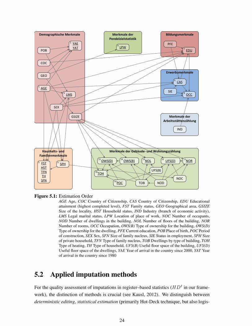
PFE

NOCNOD

UFS(B)

TOB

SIE

POB

COC

GEO

SEX

GSIZE

IND

Merkmale der Pendelzielstatistik

Erwerbsmerkmale

Bildungsmerkmale

Merkmale der Arbeitsstättenzählung

Haushalts- und Familienmerkmale

Merkmale der Gebäude- und Wohnungszählung

Demographische Merkmale

AGE1

YAE YAT

2

LMS4

SPH3FST

HST TFN TH

SFN

5

CAS6

EDU7

OCC8

LPW9

TOH16

POC10

OWS(D)15

OWS(B)14

NOL13

UFS(D)12

NOR11

Figure 5.1: Estimation OrderAGE Age, COC Country of Citizenship, CAS Country of Citizenship, EDU Educationalattainment (highest completed level), FST Family status, GEO Geographical area, GSIZESize of the locality, HST Household status, IND Industry (branch of economic activity),LMS Legal marital status, LPW Location of place of work, NOC Number of occupants,NOD Number of dwellings in the building, NOL Number of floors of the building, NORNumber of rooms, OCC Occupation, OWS(B) Type of ownership for the building, OWS(D)Type of ownership for the dwelling, PFE Current education, POB Place of birth, POC Periodof construction, SEX Sex, SFN Size of family nucleus, SIE Status in employment, SPH Sizeof private household, TFN Type of family nucleus, TOB Dwellings by type of building, TOHType of heating, TH Type of household, UFS(B) Useful floor space of the building, UFS(D)Useful floor space of the dwellings, YAE Year of arrival in the country since 2000, YAT Yearof arrival in the country since 1980

5.2 Applied imputation methods

For the quality assessment of imputations in register–based statistics (HDI in our frame-work), the distinction of methods is crucial (see Kausl, 2012). We distinguish betweendeterministic editing, statistical estimation (primarily Hot-Deck technique, but also logis-

24

tic regressions) and statistical matching. To begin with the first, missing values in the datacan be imputed by deterministic rules, even before applying statistical methods becausewe are able to derive missing values from auxiliary data. Two examples from the Austrianregister–based census illustrate such cases:

• Missing values in the legal marital status (LMS) are classified according to the Cen-tral Social Security Register. Information on individuals receiving a widow’s orwidower’s pension is provided by this register. The relevant information is gatheredto change missing values of the attribute LMS to “widowed”, if a person receives awidow’s or widower’s pension.

• People younger than 15 years are classified “not applicable (persons under 15 yearsof age)” with regard to the educational attainment (EDU). Their current activitystatus (CAS) is “persons below the age of 15” and their marital status (LMS) is“never married”.

We do not consider such derivations with the utmost matching probability as an es-timation in the narrower sense but rather as plausibility steps. However, there are alsoderivations with substantial uncertainty due to a lack of information. Still, in the follow-ing cases taken from the Austrian register–based census no statistical imputation methodis necessary:

• The Central Population Register has information on the place of birth (POB). Miss-ing values are filled up with information on the country of citizenship (COC), ifthe person has a foreign citizenship. The available data justify this assumption:77% of individuals with a foreign COC were also born in this (foreign) country.Hence, even though there is uncertainty, this imputation method classifies 77% ofthe attribute POB as correct when it is applied to observed data for 2011.

• Suppose the marital status (LMS) is missing and there is another individual living inthe same household. If the other person is “married”, the age difference betweenthe two individuals is less than 18 years, and their sex differs, then the missingmarital status is set to “married”.

Another important imputation method for the Austrian census is Hot-deck imputation.This method choses the imputed value from an assumed or estimated distribution, thatis taken from existing data (Little & Rubin, 2002). It is suitable for all scenarios ofmissing data, except for missing not at random higher than 10% (Roth, 1994). A detailedreview on hot-deck methods is given by Andridge and Little (2010). For the Austrian caseindividuals are aggregated to groups (“decks”) by attributes which are strongly correlatedto the response variable. The distribution in the decks of the source data, derived fromthe FDP, is transferred to the corresponding group of the target data. Table 5.1 gives an

25

example of artificial data for the LMS. The distribution of the existing values in the censusof the same year is applied on the missing values for the same attribute. As an example,55.6% of all females aged 30 to 40 years with their main residence in the federal stateTyrol and a missing value for LMS will be considered as married women. Since we cannotbe sure which women with a missing LMS are actually married, a uniformly distributedrandom variable with the interval [0,1] determines the assignment of the LMS. Accordingto our example in Table 5.1, the interval [0,0.37) is assigned to “LMS never married”,the interval [0.37,0.926) is assigned to “married”, the interval [0.926,0.996) is assigned“divorced” and finally the interval [0.996,1) is assigned to “widowed”.

Table 5.1: Artificial example of the Deck for legal marital status (LMS)

Sex Age Federal State Size of deck Pnevermarried Pmarried Pdivorced Pwidowed

female 30-40 Tyrol 50.000 37% 55.6% 7% 0.4%male 50-60 Vienna 100.000 12% 66% 20% 2%

......

......

......

......

Finally, statistical matching is the last applied imputation method in the Austrian cen-sus. It is based on the combination of two incomplete records. We will explain the pro-cedure using an example of a missing observation for the educational attainment (EDU).Register–based statistics rely on unique identification keys for every individual in orderto combine the information from multiple data sources. Consider a data record with amissing value for the educational attainment (EDU). Consider another data record witha missing unique identification key but information on several other attributes, amongwhich is the (EDU). Statistical matching searches these loose observations and connectsthem with individuals who have a missing value for EDU but else the same characteris-tics. Two incomplete records, one of them useless because of the missing identificationkey, can be merged to one complete record.

5.3 Quality assessment of imputation models

In general an overall quality measure for imputations requires the evaluation of two parts,the input of the estimation model as well as the output (i.e. the accuracy of the model).The inputs of the estimation models are assessed with the three hyperdimensions HDD,HDP , and HDE that are combined in the CDB.

For the evaluation of the model itself, the so–called classification rate Φ is used toobtain a quality measure for the imputations.1 It is a general measure for the goodnessof fit and can also be calculated for a variety of imputation techniques. Its principle is

1The statistical measures to evaluate the imputation performance were adopted from Hui and AlDarmaki(2012) as well as Chambers (2001).

26

to apply the imputation model to already existing data and compare the results of theimputation process with the true values of these observations. The classification rateequals the ratio between the matching values and the number of all compared entries.

This measure can be applied specifically to categorical variables and is shown in equa-tion (5.1), where Yi is the estimated value for the observed value Y ∗i of person i. n is thesample size and I is an indicator function. Take the legal marital status (LMS) as an ex-ample for a categorical variable. In this case the quality assessment should measure thehit ratio, i.e. the probability that the estimation model picks exactly the right category ofthe true value.

Φm = 1− n−1

N∑j=1

I(Yj 6= Y ∗j ) (5.1)

For ordinal variables, the distance of the imputed value to the true value is relevant,hence equation (5.2) is a modification of the classification rate Φ that measures and stan-dardizes this gap. A satisfactory quality indicator has to consider the accuracy of themodel which means measuring the contiguity of the estimated value to the true value.Assume several categories of the attribute educational attainment (EDU), ranging fromprimary to higher tertiary education. If the true value was higher tertiary education, anestimated value of lower tertiary education would be more accurate than an estimatedvalue of lower secondary education.

Φm = 1− n−1

N∑j=1

(1

2

[|Yj − Y ∗j |

max(Y )−min(Y )+ I(Yj 6= Y ∗j )

])(5.2)

For the case of numerical variables both concepts (5.1) and (5.2) can be applied,2

however a simple correlation coefficient between estimated and true values is consideredto be a rather intuitive approach. One example for a metric attribute is the variable “usefulfloor space” (UFS) of a household. The correlation coefficient between the estimated andthe true UFS can be applied analogously to the classification rate for the evaluation of theimputation model.

Finally, we explain the application of the assessment of imputation methods describedabove: deterministic editing with and without uncertainty, statistical estimation as wellas statistical matching. As already mentioned, the source variables for the imputationprocess are the attributes in the FDP rather than attributes in the raw data. Therefore,the quality indicator from the FDP delivers the quality information for the source vari-ables whereby we use the values for the single statistical units. According to the type ofimputation we distinguish the following quality assessment rules:

2Chambers (2001, p. 15) suggests that the methods which are developed for categorical variables couldalso be applied on scalar attributes by first categorizing them. If the arbitrariness of categorizing variablesshould be avoided, an applicable imputation performance measure has to be constructed.

27

• Deterministic editing without uncertainty: The input quality equals the qualityof the source variables qΩ,i where i denotes the attribute. The output quality equals1, as there is no uncertainty about the correctness of the model. The overall qualityof the imputation yields

HDIn = Φ · 1

n

N∑j=1

qnΩ,i︸ ︷︷ ︸qnInput

(5.3)

where Φ = 1.

• Deterministic editing with uncertainty: The input quality equals again the aver-age quality of the source variables qΩ,i, while the output quality equals the classifi-cation rate Φ, as shown in equation (5.3).

• Statistical estimation: We define imputation quality as the average quality of thepredictors qΩ,i (input quality) times the classification rate (output quality) for theimputations (see again equation 5.3). This measure is independent of the numberof predictors and includes both the quality of the data used for the imputations aswell as their ex–post fit.

• Statistical matching: Two incomplete records — one without unique identificationkey, another one with the missing value — are merged. Therefore, no imputation inthe narrower sense is carried out. The formerly missing value in the merged recordsis from now on treated as any other non–missing value. The quality measure isobtained via the quality of the used data source.

28

Chapter 6

Conclusion

The comprehensive quality-framework enables to assess the quality of data in every stepof the data-generation. Even though it was developed around the first register-based cen-sus in Austria, the aim was to realize a generalizable procedure for the evaluation of allkind of administrative data. According to theoretical considerations, the weights can bechosen and due to the modular design, each step can be carried out individually. Theapplication of the quality framework for the register-based census comprises various pos-sibilities. From one final quality indicator the user can decompose the value and findthe underlaying quality related information. As the quality indicator is calculated on thelevel of statistical units data quality can be analyzed for sub-groups of the census. Fur-thermore, it can be used as an additional factor of uncertainty in statistical analysis. Thepossibility to use the quality indicator for statistical purposes is, however, still an ongoingresearch task. A very simple, but nevertheless important application is the comparisonand monitoring of data-quality. Both, between different data sources and between differ-ent census-years.

The detailed results for the Austrian census of 2011 can be downloaded from theHomepage of Statistics Austria.1

1http://www.statistik.at/web_de/Redirect/index.htm?dDocName=076880

29

References

Andridge, R. R., & Little, R. J. A. (2010). A review of hot deck imputation for surveynon-response. International Statistical Review, Volume 78, Number 1, 40-64.

Astleithner, F., Cetkovic, P., Humer, S., Lenk, M., Moser, M., Schnetzer, M., et al. (forth-coming). Quality measurement in administrative statistics and the assessment ofimputations. Journal of Official Statistics.

Axelson, M., Holmberg, A., Jansson, I., Werner, P., & Westling, S. (2012). Doing aregister-based census for the first time: The swedish experiences. In A. S. Associ-ation (Ed.), Jsm proceedings, survey statistics section (p. 1473-1480).

Batini, C., & Scannapieco, M. (2006). Data quality: concepts, methodologies and tech-niques. Springer.

Berka, C., Humer, S., Lenk, M., Moser, M., Rechta, H., & Schwerer, E. (2010). A QualityFramework for Statistics based on Administrative Data Sources using the Exampleof the Austrian Census 2011. Austrian Journal of Statistics, Volume 39, Number 4,299-308.

Berka, C., Humer, S., Lenk, M., Moser, M., Rechta, H., & Schwerer, E. (2012). Combi-nation of evidence from multiple administrative data sources: quality assessment ofthe Austrian register-based census 2011. Statistica Neerlandica, Volume 66, Issue1, 18-33.

Chambers, R. (2001). Evaluation criteria for statistical editing and imputation. NationalStatistics Methodological Series No. 28.

Daas, P., & Fonville, T. (2007). Quality control of dutch administrative registers: Aninventory of quality aspects (Tech. Rep.). Statistics Netherlands.

Daas, P., Ossen, S., Vis-Visschers, R., & Arends-Tóth, J. (2009). Checklist for thequality evaluation of administrative data sources. Statistics Netherlands DiscussionPaper(09042).

Daas, P. J., Ossen, S. J., Tennekes, M., & Nordholt, E. S. (2012). Evaluation of the qualityof administrative data used in the dutch virtual census. In A. S. Association (Ed.),Jsm proceedings, survey statistics section (p. 1462-1472).

Dempster, A. (1967). Upper and lower probabilities induced by a multivariate mapping.Annals of Mathematical Statistics, 38, 325–339.

Dempster, A. (1968). A generalization of bayesian inference. Journal of the Royal

30

Statistical Society. Series B (Methodological), 30(2), 205–247.European Commission. (2010). Commission Regulation (EU) No 1151/2010. Official

Journal of the European Union, Volume 53, L 324.Hacking, I. (1975). The emergence of probability: A philosophical study of early ideas

about probability, induction and statistical inference.Helton, J. (1997). Uncertainty and sensitivity analysis in the presence of stochastic and

subjective uncertainty. Journal of Statistical Compution and Simulation, 57, 3–76.Hendriks, C. (2012). Input data quality in register based statistics – the norwegian ex-

perience. In A. S. Association (Ed.), Jsm proceedings, survey statistics section(p. 1473-1480).

Hui, G., & AlDarmaki, H. I. (2012). Editing and Imputation of the 2011 Abu Dhabi Cen-sus. Conference contribution at UNECE Work Session on Statistical Data Editing,Oslo, 24-26 September 2012.

Joshi, A., Sahasarabudhe, S., & Shankar, K. (1995). Sensitivity of combination schemesunder conflicting conditions and a new method. In J. Wainer & A. Carvalho (Eds.),Advances in artificial intelligence: 12th brazilian symposium on artificial intelli-gence. Springer.

Karr, A., Sanil, A., & Banks, D. (2006). Data quality: A statistical perspective. StatisticalMethodology, 3(2), 137–173.

Kausl, A. (2012). The data imputation process of the Austrian register-based census.Conference contribution at UNECE Work Session on Statistical Data Editing, Oslo,24-26 September 2012.

Lenk, M. (2008). Methods of Register-based Census in Austria (Tech. Rep.). StatistikAustria, Wien.

Little, R. J. A., & Rubin, D. B. (2002). Statistical analysis with missing data. Wiley.Pipino, L. L., Lee, Y. W., & Wang, R. Y. (2002). Data quality assessment. Communica-

tions of the ACM, 45(4).Roth, P. L. (1994). Missing data: A conceptual review for applied psychologists. Per-

sonnel Psychology, 47(3), 537-560.Sentz, K., & Ferson, S. (2002). Combination of evidence in dempster–shafer theory.

Sandia National Laboratories.Shafer, G. (1992). Dempster-Shafer Theory. In S. C. Shapiro (Ed.), Encyclopedia of

artificial intelligence (p. 330-331). Wiley.UNECE. (2007). Register based statistics in the Nordic countries. Review on best prac-

tices with focus on population and social statistics (Tech. Rep.). United NationsEconomic Commission for Europe.

UNECE. (2014). Measuring population and housing – Practices of UNECE countries inthe 2010 round of censuses (Tech. Rep.). United Nations Economic Commissionfor Europe.

31

Wallgren, A., & Wallgren, B. (2007). Register–based statistics. John Wiley & Sons, Ltd.Yager, R. (1987). On the dempster-shafer framework and new combination rules. Infor-

mation sciences, 41(2), 93–137.Zadeh, L. (1965). Fuzzy sets. Information and control, 8(3), 338–353.Zadeh, L. (1986). A simple view of the dempster-shafer theory of evidence and its

implication for the rule of combination. AI magazine, 7(2), 85.Zhang, L.-C. (2011). A unit-error theory for register-based household statistics. Journal

of Official Statistics, 27(3), 415–432.Zhang, L.-C. (2012). Topics of statistical theory for register-based statistics and data

integration. Statistica Neerlandica, 66(1), 41–63.

32

Appendix A

Translations

33

Tabl

eA

.1:T

rans

latio

nof

the

Ger

man

nam

esfo

rRaw

-dat

a

Ger

man

Abb

revi

atio

nFu

llG

erm

anN

ame

Eng

lish

Abb

revi

atio

nFu

llE

nglis

hN

ame

Dem

ogra

fieD

emog

raph

yD

EM

_ALT

ER

Alte

rin

Jahr

enA

GE

Age

DE

M_F

AM

STFa

mili

enst

and

LM

SL

egal

Mar

italS

tatu

sD

EM

_GE

BST

AA

TG

ebur

tsla

ndPO

BC

ount

ry/p

lace

ofbi

rth

DE

M_S

TAA

TB

Staa

tsan

gehö

rigk

eit

CO

CC

ount

ryof

citiz

ensh

ipD

EM

_ZU

WA

N_1

980

Jahr

derA

nkun

ftim

Mel

dela

ndse

it19

80YA

EY

earo

farr

ival

inth

eco

untr

ysi

nce

1980

DE

M_Z

UW

AN

_200

0Ja

hrde

rAnk

unft

imM

elde

land

seit

2000

YAT

Yea

rofa

rriv

alin

the

coun

try

sinc

e20

00B

EZ

Bez

iehu

ngen

zwis

chen

den

Hau

shal

tsm

itglie

dern

RH

MR

elat

ion

ofho

useh

old

mem

bers

GK

Z_H

WS

Übl

iche

rAuf

enth

alts

ort

GE

OPl

ace

ofus

ualr

esid

ence

Aus

bild

ung

Edu

catio

nE

DU

_HA

B_A

BFE

LD

_NA

TFe

ldde

shö

chst

enab

gesc

hlos

sene

nB

ildun

gsni

veau

sFi

eld

ofhi

ghes

tedu

catio

nala

ttain

men

tE

DU

_HA

B_N

AT

Höc

hste

sab

gesc

hlos

sene

sB

ildun

gsni

veau

ED

UE

duca

tiona

latta

inm

ent(

high

estc

ompl

eted

leve

l)E

DU

_WL

AU

_AB

FEL

DW

icht

igst

ela

ufen

deA

usbi

ldun

gM

osti

mpo

rtan

tcur

rent

educ

atio

nE

rwer

bstä

titig

keit

Em

ploy

men

tE

RW

_GE

RIN

GF

Ger

ingf

ügig

Min

orem

ploy

men

tE

RW

_STA

TU

SD

erze

itige

rErw

erbs

stat

usC

AS

Cur

rent

activ

ityst

atus

ER

W_V

TB

ESC

HVo

ll/Te

ilzei

tFu

ll-Ti

me

orPa

rt-T

ime

Arb

eits

stät

ten

und

Unt

erne

hmun

gen

Ent

erpr

ises

and

thei

rlo

calu

nits

KZ

A_G

KZ

Gem

eind

eken

nziff

erde

rArb

eits

stät

teL

PWL

ocat

ion

plac

eof

wor

k(l

ocal

unit)

KZ

A_O

EN

AC

EÖ

NA

CE

des

Unt

erne

hmen

sIN

DIn

dust

ry(b

ranc

hof

econ

omic

activ

ity)

KZ

A_S

EL

BST

Anz

ahld

erSe

lbst

stän

dige

nan

derA

rbei

tstä

tteSe

lf-e

mpl

oyed

atth

elo

calu

nit

KZ

A_U

NSE

LB

STA

nzah

lUns

elbs

tstä

ndig

eim

Unt

erne

hmen

Em

ploy

ees

atth

eth

elo

calu

nit

KZ

U_G

KZ

ÖN

AC

Ede

sU

nter

nehm

ens

IND

Indu

stry

(bra

nch

ofec

onom

icac

tivity

)K

ZU

_RF

Rec

htsf

orm

des

Unt

erne

hmen

sL

egal

form

ofth

een

terp

rise

KZ

U_S

EL

BST

Anz

ahld

erSe

lbst

stän

dige

nim

Unt

erne

hmen

Self

-em

ploy

edat

the

ente

rpri

seK

ZU

_UN

SEL

BST

Anz

ahlU

nsel

bsts

tänd

ige

imU

nter

nehm

enE

mpl

oyee

sat

the

ente

rpri

seW

ohnu

ngen

und

Nut

zung

sein

heite

nD

wel

lings

and

othe

run

itsof

build

ings

NT

Z_A

NZ

RA

UM

Anz

ahld

erR

äum

ein

derW

ohnu

ngN

OR

Num

bero

froo

ms

NT

Z_B

AD

Vorh

ande

nsei

nei

nes

Bad

ezim

mer

sod

erei

nerD

usch

ecke

BA

TB

athi

ngfa

cilit

ies

NT

Z_G

KZ

Gem

eind

eken

nziff

erG

EO

Geo

grap

hica

lare

aN

TZ

_NT

ZA

RT

Typ

derN

utzu

ngse

inhe

itTy

peof

Dw

ellin

gN

TZ

-NT

ZFL

Nut

zfläc

heU

FSU

sefu

lfloo

rspa

ceN

TZ

-RE

CH

TSV

ER

HE

igen

tum

styp

derN

utzu

ngse

inhe

itO

WS

Leg

alfo

rmof

the

dwel

ling

NT

Z_T

OI

Vorh

ande

nsei

nei

nes

WC

sTO

ITo

iletf

acili

ties

Geb

äude

Bui

ldin

gsO

BJ_

AN

SGE

SCH

OA

nzah

lder

ober

irdi

sche

nG

esch

oße

Num

bero

ffloo

rsO

BJ_

BA

UP

Bau

peri

ode

POC

Peri

odof

cons

truc

tion

OB

J_E

IGG

ebäu

deei

gent

ümer

typ

OW

STy

peof

owne

rshi

pO

BJ_

FLN

utzfl

äche

des

Geb

äude

sU

FSU

sefu

lfloo

rspa

ceO

BJ_

GK

ZG

emei

ndek

ennz

iffer

GE

OG

eogr

aphi

cala

rea

OB

J_ST

AT

US

Geb

äude

stat

usSt

atus

ofth

ebu

ildin

g

34

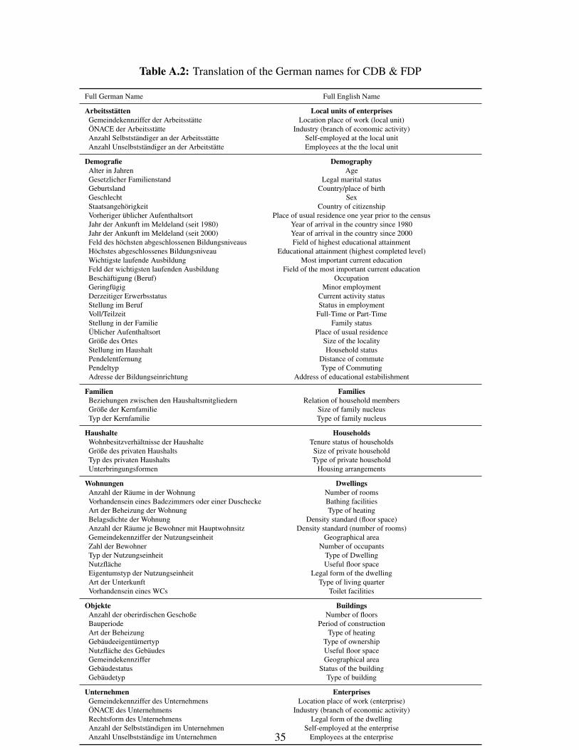
Table A.2: Translation of the German names for CDB & FDP

Full German Name Full English Name

Arbeitsstätten Local units of enterprisesGemeindekennziffer der Arbeitsstätte Location place of work (local unit)ÖNACE der Arbeitsstätte Industry (branch of economic activity)Anzahl Selbstständiger an der Arbeitsstätte Self-employed at the local unitAnzahl Unselbstständiger an der Arbeitstätte Employees at the the local unit

Demografie DemographyAlter in Jahren AgeGesetzlicher Familienstand Legal marital statusGeburtsland Country/place of birthGeschlecht SexStaatsangehörigkeit Country of citizenshipVorheriger üblicher Aufenthaltsort Place of usual residence one year prior to the censusJahr der Ankunft im Meldeland (seit 1980) Year of arrival in the country since 1980Jahr der Ankunft im Meldeland (seit 2000) Year of arrival in the country since 2000Feld des höchsten abgeschlossenen Bildungsniveaus Field of highest educational attainmentHöchstes abgeschlossenes Bildungsniveau Educational attainment (highest completed level)Wichtigste laufende Ausbildung Most important current educationFeld der wichtigsten laufenden Ausbildung Field of the most important current educationBeschäftigung (Beruf) OccupationGeringfügig Minor employmentDerzeitiger Erwerbsstatus Current activity statusStellung im Beruf Status in employmentVoll/Teilzeit Full-Time or Part-TimeStellung in der Familie Family statusÜblicher Aufenthaltsort Place of usual residenceGröße des Ortes Size of the localityStellung im Haushalt Household statusPendelentfernung Distance of commutePendeltyp Type of CommutingAdresse der Bildungseinrichtung Address of educational estabilishment

Familien FamiliesBeziehungen zwischen den Haushaltsmitgliedern Relation of household membersGröße der Kernfamilie Size of family nucleusTyp der Kernfamilie Type of family nucleus

Haushalte HouseholdsWohnbesitzverhältnisse der Haushalte Tenure status of householdsGröße des privaten Haushalts Size of private householdTyp des privaten Haushalts Type of private householdUnterbringungsformen Housing arrangements

Wohnungen DwellingsAnzahl der Räume in der Wohnung Number of roomsVorhandensein eines Badezimmers oder einer Duschecke Bathing facilitiesArt der Beheizung der Wohnung Type of heatingBelagsdichte der Wohnung Density standard (floor space)Anzahl der Räume je Bewohner mit Hauptwohnsitz Density standard (number of rooms)Gemeindekennziffer der Nutzungseinheit Geographical areaZahl der Bewohner Number of occupantsTyp der Nutzungseinheit Type of DwellingNutzfläche Useful floor spaceEigentumstyp der Nutzungseinheit Legal form of the dwellingArt der Unterkunft Type of living quarterVorhandensein eines WCs Toilet facilities

Objekte BuildingsAnzahl der oberirdischen Geschoße Number of floorsBauperiode Period of constructionArt der Beheizung Type of heatingGebäudeeigentümertyp Type of ownershipNutzfläche des Gebäudes Useful floor spaceGemeindekennziffer Geographical areaGebäudestatus Status of the buildingGebäudetyp Type of building

Unternehmen EnterprisesGemeindekennziffer des Unternehmens Location place of work (enterprise)ÖNACE des Unternehmens Industry (branch of economic activity)Rechtsform des Unternehmens Legal form of the dwellingAnzahl der Selbstständigen im Unternehmen Self-employed at the enterpriseAnzahl Unselbstständige im Unternehmen Employees at the enterprise35