Embed Size (px)
Citation preview
The Pennsylvania State University
The Graduate School
Department of Electrical Engineering
QR SIGNAL DETECTION IN THE
PRESENCE OF AM NOISE
A Dissertation in
Electrical Engineering
by
Abdullah G. Almahri
c© 2013 Abdullah G. Almahri
Submitted in Partial Fulfillmentof the Requirements
for the Degree of
Doctor of Philosophy
December 2013
The dissertation of Abdullah G. Almahri was reviewed and approved* by the following:
Constantino C. LagoaProfessor of Electrical EngineeringDissertation AdviserChair of Committee
Jeffrey SchianoProfessor of Electrical Engineering
David MillerProfessor of Electrical Engineering
Patrick M. LenahanProfessor of Engineering Science and Mechanics
Kultegin AydinProfessor of Electrical EngineeringHead of the Department of Electrical Engineering
*Signatures are on file in the Graduate School.
iii
Abstract
The thesis proposes a matched filter approach to detect quadrupole resonance (QR)
signals in the presence of disturbance from AM stations. Detecting QR signals is a
challenge due to several reasons. One is the amplitude of a QR signal is typically on
the same level of thermal noise, which makes it very susceptible to noise interferences.
External Radio Frequency (RF) interferences, such as AM signals, and internal RF
interferences, ones from inside the search volume, pose another challenge and contribute
to the low SNR values observed. AM stations broadcast within the same frequency band
of QR signals, which is a problem for QR detection. A third important challenge we face
is the uncertainty in the QR signal characteristics.
To motivate the use of a matched filter approach, a matched filter (under the assumption
that the QR signal is known) was compared to the generic energy detector in theory and it
resulted in a performance improvement. The work proposes a detector referred to as the
batch matched filter, which uses a gridding technique to search for unknown QR signal
parameters and attempts to match the filter to the shape of the QR signal present. This
approach resulted in a performance gain when compared to the generic energy detector
using simulation and experimental data, where the QR signal is unknown. To further
improve performance we introduced an approach that would also match the filter to the
noise present in addition to the QR signal. This approach is referred to as the batch
whitened matched filter and when properly matched to the noise outperforms both the
batch matched filter and energy detector.
iv
Table of Contents
List of Tables . . . . . . . . . . . . . . . . . . . . . . . . . . . . . . . . . . . . . . vii
List of Figures . . . . . . . . . . . . . . . . . . . . . . . . . . . . . . . . . . . . . ix
Acknowledgments . . . . . . . . . . . . . . . . . . . . . . . . . . . . . . . . . . . xviii
Chapter 1. Introduction . . . . . . . . . . . . . . . . . . . . . . . . . . . . . . . . 11.1 Motivation . . . . . . . . . . . . . . . . . . . . . . . . . . . . . . . . . 11.2 Literature Review . . . . . . . . . . . . . . . . . . . . . . . . . . . . . 21.3 Approach . . . . . . . . . . . . . . . . . . . . . . . . . . . . . . . . . 10
Chapter 2. QR Spectroscopy . . . . . . . . . . . . . . . . . . . . . . . . . . . . . 122.1 QR Physics . . . . . . . . . . . . . . . . . . . . . . . . . . . . . . . . 13
2.1.1 Quadrupole Interaction . . . . . . . . . . . . . . . . . . . . . 132.1.2 Relaxation Mechanisms . . . . . . . . . . . . . . . . . . . . . 19
2.2 Observed Signals . . . . . . . . . . . . . . . . . . . . . . . . . . . . . 202.3 RF Excitation Pulse Sequences . . . . . . . . . . . . . . . . . . . . . 202.4 QR Detection Procedure . . . . . . . . . . . . . . . . . . . . . . . . . 22
Chapter 3. Challenges, Signal Characteristics and Data Generation . . . . . . . 253.1 Challenges . . . . . . . . . . . . . . . . . . . . . . . . . . . . . . . . . 25
3.1.1 Challenges Due to Uncertainty QR Signal . . . . . . . . . . . 253.1.2 Challenges Due to External and Internal RFI Signals . . . . . 28
3.2 RFI Mitigation Methods . . . . . . . . . . . . . . . . . . . . . . . . . 313.3 QR Signals . . . . . . . . . . . . . . . . . . . . . . . . . . . . . . . . 323.4 Noise Characteristics . . . . . . . . . . . . . . . . . . . . . . . . . . . 36
3.4.1 Thermal Noise . . . . . . . . . . . . . . . . . . . . . . . . . . 363.4.2 AM Signals . . . . . . . . . . . . . . . . . . . . . . . . . . . . 37
3.5 Averaged Nm Trials . . . . . . . . . . . . . . . . . . . . . . . . . . . 383.6 Aggregating Nm Trials . . . . . . . . . . . . . . . . . . . . . . . . . . 393.7 Experimental Data Versus Simulation Data . . . . . . . . . . . . . . 41
3.7.1 Experimental Data Collected . . . . . . . . . . . . . . . . . . 413.7.2 Simulation Data Generated . . . . . . . . . . . . . . . . . . . 42
Chapter 4. Motivation for Using Matched Filter . . . . . . . . . . . . . . . . . . 444.1 Energy Detector . . . . . . . . . . . . . . . . . . . . . . . . . . . . . 474.2 Matched Filter . . . . . . . . . . . . . . . . . . . . . . . . . . . . . . 474.3 Detection Algorithm Comparison Under Noise Assumptions . . . . . 50
4.3.1 Energy Detector in the Presence of Thermal Noise . . . . . . 534.3.2 Energy Detector in the Presence of AM and Thermal Noise . 564.3.3 Matched Filter in the Presence of Thermal Noise . . . . . . . 60
v
4.3.4 Matched Filter in the Presence of AM and Thermal Noise . . 634.3.5 Thermal Noise Comparison . . . . . . . . . . . . . . . . . . . 674.3.6 AM and Thermal Noise Comparison . . . . . . . . . . . . . . 68
4.4 Algorithm Comparison, No Noise Assumptions . . . . . . . . . . . . 694.4.1 Band and Low pass Filtered Thermal Noise . . . . . . . . . . 704.4.2 Band and Low pass Filtered AM and Thermal Noise . . . . . 73
4.5 Conclusion . . . . . . . . . . . . . . . . . . . . . . . . . . . . . . . . . 78
Chapter 5. Batch Matched Filter . . . . . . . . . . . . . . . . . . . . . . . . . . . 795.1 Error in the QR signal Description . . . . . . . . . . . . . . . . . . . 815.2 Batch Matched Filter . . . . . . . . . . . . . . . . . . . . . . . . . . . 865.3 Batch Matched Filter versus Energy Detector, Unknown QR signal . 90
5.3.1 Simulation Data . . . . . . . . . . . . . . . . . . . . . . . . . 915.3.2 Experimental Data . . . . . . . . . . . . . . . . . . . . . . . . 91
5.4 The Effect of Finer Gridding on the Performance of the Batch MatchedFilter . . . . . . . . . . . . . . . . . . . . . . . . . . . . . . . . . . . . 95
5.5 Adaptive Grid Batch Matched Filter . . . . . . . . . . . . . . . . . . 985.5.1 Simulation Data . . . . . . . . . . . . . . . . . . . . . . . . . 1015.5.2 Experimental Data . . . . . . . . . . . . . . . . . . . . . . . . 102
5.6 Alternative Detection Decisions . . . . . . . . . . . . . . . . . . . . . 107
Chapter 6. Batch Whitened Matched Filter . . . . . . . . . . . . . . . . . . . . . 1166.1 Whitened Matched Filter . . . . . . . . . . . . . . . . . . . . . . . . 117
6.1.1 Estimating Whitening Matrix using the Autocorrelation Method 1216.1.2 Estimating Whitening Matrix using the Covariance Method . 1236.1.3 The Effect of All Zero Filters On a QR Signal . . . . . . . . . 125
6.2 Batch Whitened Matched Filter . . . . . . . . . . . . . . . . . . . . . 1296.3 Batch Whitened Matched Filter versus Energy Detector, Unknown
QR signal . . . . . . . . . . . . . . . . . . . . . . . . . . . . . . . . . 1356.3.1 Simulation Data . . . . . . . . . . . . . . . . . . . . . . . . . 1356.3.2 Experimental Data . . . . . . . . . . . . . . . . . . . . . . . . 152
6.4 Batch Adaptive Whitened Matched Filter . . . . . . . . . . . . . . . 1686.4.1 Whitening Filter Order that Least Effects the QR Signal . . . 1746.4.2 Whitening Filter Order, Minimum Description Length Algo-
rithm . . . . . . . . . . . . . . . . . . . . . . . . . . . . . . . 1766.4.3 Simulation Data . . . . . . . . . . . . . . . . . . . . . . . . . 1776.4.4 Experimental Data . . . . . . . . . . . . . . . . . . . . . . . . 186
Chapter 7. Batch Whitened Robust Matched Filter . . . . . . . . . . . . . . . . 1937.1 Robust Matched Filter . . . . . . . . . . . . . . . . . . . . . . . . . . 1967.2 Analytical Solutions For Robust Matched Filters Over Particular Un-
certainty Sets . . . . . . . . . . . . . . . . . . . . . . . . . . . . . . . 2007.2.1 Spherical Signal Set and Noise Uncertainty Bounded by a Ma-
trix Norm . . . . . . . . . . . . . . . . . . . . . . . . . . . . . 201
vi
7.2.2 Elliptic Signal Set and Noise Uncertainty Bounded by theFrobenius Matrix Norm or the 2-Norm . . . . . . . . . . . . . 202
7.3 The Scenario Approach . . . . . . . . . . . . . . . . . . . . . . . . . 2077.4 Characterizing a Set of QR Signals Through Sampling . . . . . . . . 208
7.4.1 Smallest Sphere Containing the Set of QR Signals . . . . . . 2097.4.1.1 Spherical Set Central Signal Examples . . . . . . . . 211
7.5 Robust Matched Filter by Maximizing SNR Using Sampling . . . . . 2167.5.1 Robust Matched Filter Examples in the presence of Thermal
Noise, Maximizing SNR . . . . . . . . . . . . . . . . . . . . . 2187.6 Batch Whitened Robust Matched Filter . . . . . . . . . . . . . . . . 2227.7 Batch Robust Matched Filter in Presence of Thermal Noise . . . . . 227
7.7.1 Frequency Robust Batch Matched Filters in the Presence ofThermal Noise . . . . . . . . . . . . . . . . . . . . . . . . . . 228
7.7.2 Robust Batch Matched Filters in the Presence of Thermal Noise 2307.8 Batch Whitened Robust Matched Filter in the Presence of AM and
Thermal Noise . . . . . . . . . . . . . . . . . . . . . . . . . . . . . . 2337.8.1 Simulation Data in the Presence of AM and Thermal Noise . 2337.8.2 Experimental Data in the Presence of AM and Thermal Noise 237
Chapter 8. Conclusion . . . . . . . . . . . . . . . . . . . . . . . . . . . . . . . . . 2418.1 Future Work . . . . . . . . . . . . . . . . . . . . . . . . . . . . . . . 244
Appendix A. Mean and Variance of Energy Detector Test Statistic, in the Presenceof AM and Thermal Noise . . . . . . . . . . . . . . . . . . . . . . . . 246
Appendix B. Mean and Variance of Matched Filter Test Statistic, in the Presenceof AM and Thermal Noise . . . . . . . . . . . . . . . . . . . . . . . . 256
Appendix C. MATLAB Code . . . . . . . . . . . . . . . . . . . . . . . . . . . . . 259C.1 Data Generation Function . . . . . . . . . . . . . . . . . . . . . . . . 259
Bibliography . . . . . . . . . . . . . . . . . . . . . . . . . . . . . . . . . . . . . . 274
vii
List of Tables
6.1 Simulation, SNR = -22 dB, Performance Comparison on SimulationData, Band-passed White Gaussian AM, with the QR and AM at 2.5kHz. . . . . . . . . . . . . . . . . . . . . . . . . . . . . . . . . . . . . . . 137
6.2 Simulation, SNR = -22 dB, Performance Comparison on SimulationData, Band-passed White Gaussian AM, with the QR and AM at 5kHz. . . . . . . . . . . . . . . . . . . . . . . . . . . . . . . . . . . . . . . 139
6.3 Simulation, SNR = -22 dB, Performance Comparison on SimulationData, Band-passed White Gaussian AM, with the QR and AM at 7.5kHz. . . . . . . . . . . . . . . . . . . . . . . . . . . . . . . . . . . . . . . 139
6.4 Simulation, SNR = -22 dB, Performance Comparison on SimulationData, Band-passed White Gaussian AM, with the QR and AM at 10kHz. . . . . . . . . . . . . . . . . . . . . . . . . . . . . . . . . . . . . . . 140
6.5 Simulation, SNR = -22 dB, Performance Comparison on SimulationData, Band-passed White Gaussian AM, with the QR and AM at 12.5kHz. . . . . . . . . . . . . . . . . . . . . . . . . . . . . . . . . . . . . . . 141
6.6 Simulation, SNR = -22 dB, Performance Comparison on SimulationData, Band-passed White Gaussian AM, with the QR and AM at 15kHz. . . . . . . . . . . . . . . . . . . . . . . . . . . . . . . . . . . . . . . 148
6.7 Performance Comparison on Experimental Data A, BP White GaussianAM, with the QR and AM at 6.25 kHz. . . . . . . . . . . . . . . . . . . 165
6.8 Performance Comparison on Experimental Data B, BP White GaussianAM, with the QR and AM at 10 kHz. . . . . . . . . . . . . . . . . . . . 166
6.9 Performance Comparison on Experimental Data C, BP White GaussianAM, with the QR and AM at -8 kHz. . . . . . . . . . . . . . . . . . . . 167
6.10 Performance Comparison on Experimental Data D, BP White GaussianAM, with the QR and AM at 12.5 kHz. . . . . . . . . . . . . . . . . . . 167
6.11 Simulation, SNR = -22 dB, Performance Comparison on SimulationData, Band-passed White Gaussian AM, with the QR and AM at 2.5kHz. Adaptive Whitening Filter Order Selection. . . . . . . . . . . . . . 179
6.12 Simulation, SNR = -22 dB, Performance Comparison on SimulationData, Band-passed White Gaussian AM, with the QR and AM at 5kHz. Adaptive Whitening Filter Order Selection. . . . . . . . . . . . . . 179
6.13 Simulation, SNR = -22 dB, Performance Comparison on SimulationData, Band-passed White Gaussian AM, with the QR and AM at 7.5kHz. Adaptive Whitening Filter Order Selection. . . . . . . . . . . . . . 180
6.14 Simulation, SNR = -22 dB, Performance Comparison on SimulationData, Band-passed White Gaussian AM, with the QR and AM at 10kHz. Adaptive Whitening Filter Order Selection. . . . . . . . . . . . . . 181
6.15 Simulation, SNR = -22 dB, Performance Comparison on SimulationData, Band-passed White Gaussian AM, with the QR and AM at 12.5kHz. Adaptive Whitening Filter Order Selection. . . . . . . . . . . . . . 181
viii
6.16 Simulation, SNR = -22 dB, Performance Comparison on SimulationData, Band-passed White Gaussian AM, with the QR and AM at 15kHz. Adaptive Whitening Filter Order Selection. . . . . . . . . . . . . . 182
6.17 Performance Comparison on Experimental Data A, BP White GaussianAM, with the QR and AM at 6.25 kHz. Adaptive Whitening Filter OrderSelection . . . . . . . . . . . . . . . . . . . . . . . . . . . . . . . . . . . . 187
6.18 Performance Comparison on Experimental Data B, BP White GaussianAM, with the QR and AM at 10 kHz. Adaptive Whitening Filter OrderSelection . . . . . . . . . . . . . . . . . . . . . . . . . . . . . . . . . . . . 188
6.19 Performance Comparison on Experimental Data C, BP White GaussianAM, with the QR and AM at -8 kHz. Adaptive Whitening Filter OrderSelection . . . . . . . . . . . . . . . . . . . . . . . . . . . . . . . . . . . . 189
6.20 Performance Comparison on Experimental Data D, BP White GaussianAM, with the QR and AM at 12.5 kHz. Adaptive Whitening Filter OrderSelection . . . . . . . . . . . . . . . . . . . . . . . . . . . . . . . . . . . . 189
ix
List of Figures
2.1 Simplified block diagram of QR detection system . . . . . . . . . . . . . 132.2 QR energy levels and transition frequencies for nitrogen-14, an I=1 nu-
cleus with η 6= 0 [17]. . . . . . . . . . . . . . . . . . . . . . . . . . . . . . 162.3 QR frequencies of different explosives/chemicals [3] . . . . . . . . . . . . 172.4 Lorentzian distribution of transition frequencies [17]. . . . . . . . . . . . 182.5 Block diagram of QR spectrometer . . . . . . . . . . . . . . . . . . . . . 24
3.1 QR Signal with a Frequency of 3.016 MHz and T2∗ of 500e-6 . . . . . . 26
3.2 Comparison of QR+AM and QR: (Top) QR Signal with a Frequency of3.016 MHz and T2
∗ of 500e-6 (Center) AM Signal with Carrier Frequencyof 3.016 MHz (Bottom) QR plus AM Signal, SNR = -12 dB . . . . . . . 30
3.3 Illustration of Phase Cycling on SLSE sequences. . . . . . . . . . . . . . 32
4.1 Energy Detector’s Theoretical PDF plots vs Simulation PDF plots forThermal Noise, SNR = 20 log10( A
σtn) = -50 dB . . . . . . . . . . . . . . 55
4.2 Energy Detector’s, Theoretical ROC plot vs Simulation ROC plot forThermal Noise, SNR = 20 log10( A
σtn) = -50 dB . . . . . . . . . . . . . . 57
4.3 Energy Detector’s Theoretical PDF plots vs Simulation PDF plots forAM and Thermal Noise, SNR = 20 log10( A
Aη) = -66 dB . . . . . . . . . . 59
4.4 Energy Detector’s, Theoretical ROC plot vs Simulation ROC plot forAM and Thermal Noise, SNR = 20 log10( A
Aη) = -66 dB . . . . . . . . . . 61
4.5 Matched Filter’s Theoretical PDF plots vs Simulation PDF plots forThermal Noise, SNR = 20 log10( A
σtn) =-50 dB . . . . . . . . . . . . . . . 63
4.6 Theoretical ROC plot vs Simulation ROC plot for Thermal Noise, SNR= 20 log10( A
σtn) = -50 dB . . . . . . . . . . . . . . . . . . . . . . . . . . . 64
4.7 Matched Filter’s Theoretical PDF plots vs Simulation PDF plots for AMand Thermal Noise, SNR = 20 log10( A
Aη) = -66 dB . . . . . . . . . . . . 66
4.8 Theoretical ROC plot vs Simulation ROC plot for AM & Thermal Noise,SNR = 20 log10( A
Aη) = -66 dB . . . . . . . . . . . . . . . . . . . . . . . . 68
4.9 Energy of noise signals vs number of averages, Log scale. . . . . . . . . . 704.10 Energy Detector PDF plots in the presence of Thermal Noise, SNR =
20 log10( Aσtn
) =-12 dB, Theoretical PDF plots vs Simulation and Exper-iment without Noise Assumptions . . . . . . . . . . . . . . . . . . . . . . 72
4.11 Matched Filter PDF plots in the presence of Thermal Noise, SNR =20 log10( A
σtn) = -12 dB, Theoretical PDF plots vs Simulation and Exper-
iment without Noise Assumptions . . . . . . . . . . . . . . . . . . . . . . 744.12 Energy Detector PDF plots in the presence of band-passed white gaussian
AM and Thermal Noise, SNR = 20 log10( AAη
) = -30 dB, Theoretical PDFplots vs Simulation and Experiment without Noise Assumptions. Nm =10, Number of experiments = 50. . . . . . . . . . . . . . . . . . . . . . . 75
x
4.13 Energy Detector ROC plots in the presence of band-passed white gaus-sian AM Thermal Noise, SNR = 20 log10( A
Aη)= -30 dB, Theoretical PDF
plots vs Simulation and Experiment without Noise Assumptions. Nm =10, Number of experiments = 50. . . . . . . . . . . . . . . . . . . . . . . 76
4.14 Matched Filter PDF plots in the presence of band-passed white gaussianAM and Thermal Noise, SNR = 20 log10( A
Aη) = -30 dB, Theoretical PDF
plots vs Simulation and Experiment without Noise Assumptions. . . . . 774.15 Matched Filter PDF plots in the presence of band-passed white gaussian
AM and Thermal Noise, SNR = 20 log10( AAη
) = -30 dB, Theoretical PDFplots vs Simulation and Experiment without Noise Assumptions. . . . . 77
5.1 Inner Product versus Frequency Error of the Filter . . . . . . . . . . . . 835.2 Inner Product versus Phase Error of the Filter . . . . . . . . . . . . . . 845.3 Inner Product versus Decaying Parameter Error of the Filter . . . . . . 855.4 Uncertain Frequency Matched Filter ROC plots in the presence of Band-
passed White Gaussian AM, SNR = -30 dB . . . . . . . . . . . . . . . . 865.5 Batch Matched Filter with 1 kHz Frequency gridding, ROC plots in the
presence of Different QR Frequencies and Band-passed White GaussianAM, Simulation SNR = -22 dB . . . . . . . . . . . . . . . . . . . . . . . 87
5.6 Simulation SNR = -22 dB, Performance Comparison, BP White GaussianAM, with the QR and AM at 2.5 kHz . . . . . . . . . . . . . . . . . . . 92
5.7 Simulation SNR = -22 dB, Performance Comparison, BP White GaussianAM, with the QR and AM at 5 kHz . . . . . . . . . . . . . . . . . . . . 92
5.8 Simulation SNR = -22 dB, Performance Comparison, BP White GaussianAM, with the QR and AM at 7.5 kHz . . . . . . . . . . . . . . . . . . . 93
5.9 Simulation SNR = -22 dB, Performance Comparison, BP White GaussianAM, with the QR and AM at 10 kHz . . . . . . . . . . . . . . . . . . . . 93
5.10 Simulation SNR = -22 dB, Performance Comparison, BP White GaussianAM, with the QR and AM at 12.5 kHz . . . . . . . . . . . . . . . . . . . 94
5.11 Simulation SNR = -22 dB, Performance Comparison, BP White GaussianAM, with the QR and AM at 15 kHz . . . . . . . . . . . . . . . . . . . . 94
5.12 Experiment A, Performance Comparison on Experiment Data, BP WhiteGaussian AM, with the QR and AM at 6.25 kHz . . . . . . . . . . . . . 96
5.13 Experiment B, Performance Comparison on Experiment Data, BP WhiteGaussian AM, with the QR and AM at 10 kHz . . . . . . . . . . . . . . 96
5.14 Experiment C, Performance Comparison on Experiment Data, BP WhiteGaussian AM, with the QR and AM at -8 kHz . . . . . . . . . . . . . . 97
5.15 Experiment D, Performance Comparison on Experiment Data, BP WhiteGaussian AM, with the QR and AM at 12.5 kHz . . . . . . . . . . . . . 97
5.16 Simulation SNR = -22 dB, Adaptive versus “Brute Force” Gridding Per-formance Comparison, BP White Gaussian AM, with the QR and AMat 2.5 kHz . . . . . . . . . . . . . . . . . . . . . . . . . . . . . . . . . . . 103
5.17 Simulation SNR = -22 dB, Adaptive versus “Brute Force” Gridding Per-formance Comparison, BP White Gaussian AM, with the QR and AMat 5 kHz . . . . . . . . . . . . . . . . . . . . . . . . . . . . . . . . . . . . 103
xi
5.18 Simulation SNR = -22 dB, Adaptive versus “Brute Force” Gridding Per-formance Comparison, BP White Gaussian AM, with the QR and AMat 7.5 kHz . . . . . . . . . . . . . . . . . . . . . . . . . . . . . . . . . . . 104
5.19 Simulation SNR = -22 dB, Adaptive versus “Brute Force” Gridding Per-formance Comparison, BP White Gaussian AM, with the QR and AMat 10 kHz . . . . . . . . . . . . . . . . . . . . . . . . . . . . . . . . . . . 104
5.20 Simulation SNR = -22 dB, Adaptive versus “Brute Force” Gridding Per-formance Comparison, BP White Gaussian AM, with the QR and AMat 12.5 kHz . . . . . . . . . . . . . . . . . . . . . . . . . . . . . . . . . . 105
5.21 Simulation SNR = -22 dB, Adaptive versus “Brute Force” Gridding Per-formance Comparison, BP White Gaussian AM, with the QR and AMat 15 kHz . . . . . . . . . . . . . . . . . . . . . . . . . . . . . . . . . . . 105
5.22 Experiment A, Adaptive versus “Brute Force” Gridding PerformanceComparison on Experiment Data, BP White Gaussian AM, with the QRand AM at 6.25 kHz . . . . . . . . . . . . . . . . . . . . . . . . . . . . . 106
5.23 Experiment B, Adaptive versus “Brute Force” Gridding PerformanceComparison on Experiment Data, BP White Gaussian AM, with theQR and AM at 10 kHz . . . . . . . . . . . . . . . . . . . . . . . . . . . . 107
5.24 Experiment C, Adaptive versus “Brute Force” Gridding PerformanceComparison on Experiment Data, BP White Gaussian AM, with theQR and AM at -8 kHz . . . . . . . . . . . . . . . . . . . . . . . . . . . . 108
5.25 Experiment D, Adaptive versus “Brute Force” Gridding PerformanceComparison on Experiment Data, BP White Gaussian AM, with the QRand AM at 12.5 kHz . . . . . . . . . . . . . . . . . . . . . . . . . . . . . 108
5.26 Simulation SNR = -22 dB, Comparing Detection Decision Methods, BPWhite Gaussian AM, with the QR and AM at 2.5 kHz . . . . . . . . . . 110
5.27 Simulation SNR = -22 dB, Comparing Detection Decision Methods, BPWhite Gaussian AM, with the QR and AM at 5 kHz . . . . . . . . . . . 111
5.28 Simulation SNR = -22 dB, Comparing Detection Decision Methods, BPWhite Gaussian AM, with the QR and AM at 7.5 kHz . . . . . . . . . . 112
5.29 Simulation SNR = -22 dB, Comparing Detection Decision Methods, BPWhite Gaussian AM, with the QR and AM at 10 kHz . . . . . . . . . . 112
5.30 Simulation SNR = -22 dB, Comparing Detection Decision Methods, BPWhite Gaussian AM, with the QR and AM at 12.5 kHz . . . . . . . . . 113
5.31 Simulation SNR = -22 dB, Comparing Detection Decision Methods, BPWhite Gaussian AM, with the QR and AM at 15 kHz . . . . . . . . . . 113
5.32 Experiment A, Comparing Detection Decision Methods on ExperimentData, BP White Gaussian AM, with the QR and AM at 6.25 kHz. . . . 114
5.33 Experiment B, Comparing Detection Decision Methods on ExperimentData, BP White Gaussian AM, with the QR and AM at 10 kHz. . . . . 114
5.34 Experiment C, Comparing Detection Decision Methods on ExperimentData, BP White Gaussian AM, with the QR and AM at -8 kHz. . . . . 115
5.35 Experiment D, Comparing Detection Decision Methods on ExperimentData, BP White Gaussian AM, with the QR and AM at 12.5 kHz. . . . 115
xii
6.1 The output of a 6th order FIR filter applied to a simulated 12.5 kHz QRsignal is compared to the input signal. . . . . . . . . . . . . . . . . . . . 129
6.2 Magnitude of the Frequency Response of an 8 pole Butterworth filterwith a 20 kHz cutoff. . . . . . . . . . . . . . . . . . . . . . . . . . . . . . 131
6.3 Magnitude (dB) of the Frequency Response of an 8 pole Butterworthfilter with a 20 kHz cutoff. . . . . . . . . . . . . . . . . . . . . . . . . . . 131
6.4 Simulation, SNR = -22 dB, Performance Comparison on SimulationData, Band-passed White Gaussian AM, with the QR and AM at 2.5kHz. Autocorrelation Whitening Method. . . . . . . . . . . . . . . . . . 142
6.5 Simulation, SNR = -22 dB, Performance Comparison on SimulationData, Band-passed White Gaussian AM, with the QR and AM at 2.5kHz. Covariance Whitening Method. . . . . . . . . . . . . . . . . . . . . 142
6.6 Simulation, SNR = -22 dB, Performance Comparison on SimulationData, Band-passed White Gaussian AM, with the QR and AM at 5kHz. Autocorrelation Whitening Method. . . . . . . . . . . . . . . . . . 143
6.7 Simulation, SNR = -22 dB, Performance Comparison on SimulationData, Band-passed White Gaussian AM, with the QR and AM at 5kHz. Covariance Whitening Method. . . . . . . . . . . . . . . . . . . . . 143
6.8 Simulation, SNR = -22 dB, Performance Comparison on SimulationData, Band-passed White Gaussian AM, with the QR and AM at 7.5kHz. Autocorrelation Whitening Method. . . . . . . . . . . . . . . . . . 144
6.9 Simulation, SNR = -22 dB, Performance Comparison on SimulationData, Band-passed White Gaussian AM, with the QR and AM at 7.5kHz. Covariance Whitening Method. . . . . . . . . . . . . . . . . . . . . 144
6.10 Simulation, SNR = -22 dB, Performance Comparison on SimulationData, Band-passed White Gaussian AM, with the QR and AM at 10kHz. Autocorrelation Whitening Method. . . . . . . . . . . . . . . . . . 145
6.11 Simulation, SNR = -22 dB, Performance Comparison on SimulationData, Band-passed White Gaussian AM, with the QR and AM at 10kHz. Covariance Whitening Method. . . . . . . . . . . . . . . . . . . . . 145
6.12 Simulation, SNR = -22 dB, Performance Comparison on SimulationData, Band-passed White Gaussian AM, with the QR and AM at 12.5kHz. Autocorrelation Whitening Method. . . . . . . . . . . . . . . . . . 146
6.13 Simulation, SNR = -22 dB, Performance Comparison on SimulationData, Band-passed White Gaussian AM, with the QR and AM at 12.5kHz. Covariance Whitening Method. . . . . . . . . . . . . . . . . . . . . 146
6.14 Simulation, SNR = -22 dB, Performance Comparison on SimulationData, Band-passed White Gaussian AM, with the QR and AM at 15kHz. Autocorrelation Whitening Method. . . . . . . . . . . . . . . . . . 147
6.15 Simulation, SNR = -22 dB, Performance Comparison on SimulationData, Band-passed White Gaussian AM, with the QR and AM at 15kHz. Covariance Whitening Method. . . . . . . . . . . . . . . . . . . . . 147
xiii
6.16 Top: Frequency Response of Modulating Signal (Bandpassed GaussianNoise). Bottom: Frequency Response of an AM Signal with a CarrierFrequency of fc < 10 kHz. 0 = 0 Hz, 1 = fc- 40 Hz, 2 = fc+40 Hz, 3 =10 kHz - fc and 4 = fc+10 kHz. . . . . . . . . . . . . . . . . . . . . . . 152
6.17 Frequency Response of Whitening Filter When the AM Signal’s CarrierFrequency is fc < 10 kHz. 1 = fc- 40 Hz, 2 = fc+40 Hz, 3 = 10 kHz -fc and 4 = fc+10 kHz. . . . . . . . . . . . . . . . . . . . . . . . . . . . . 153
6.18 Fast Fourier Transform of a 2.5 kHz QR signal. . . . . . . . . . . . . . . 1536.19 Frequency Response of the Ne = 5 Whitening Filters of Order 3, De-
signed Using the Covariance Method. Simulation Data, SNR = -22 dB,Experiment 1 of Band-passed White Gaussian AM, with the QR and AMat 2.5 kHz Data Set. . . . . . . . . . . . . . . . . . . . . . . . . . . . . . 154
6.20 Frequency Response of the Ne = 5 Whitening Filters of Order 4, De-signed Using the Covariance Method. Simulation Data, SNR = -22 dB,Experiment 1 of Band-passed White Gaussian AM, with the QR and AMat 2.5 kHz Data Set. . . . . . . . . . . . . . . . . . . . . . . . . . . . . . 154
6.21 Frequency Response of the Ne = 5 Whitening Filters of Order 5, De-signed Using the Covariance Method. Simulation Data, SNR = -22 dB,Experiment 1 of Band-passed White Gaussian AM, with the QR and AMat 2.5 kHz Data Set. . . . . . . . . . . . . . . . . . . . . . . . . . . . . . 155
6.22 Frequency Response of the Ne = 5 Whitening Filters of Order 6, De-signed Using the Covariance Method. Simulation Data, SNR = -22 dB,Experiment 1 of Band-passed White Gaussian AM, with the QR and AMat 2.5 kHz Data Set. . . . . . . . . . . . . . . . . . . . . . . . . . . . . . 155
6.23 Frequency Response of the Ne = 5 Whitening Filters of Order 7, De-signed Using the Covariance Method. Simulation Data, SNR = -22 dB,Experiment 1 of Band-passed White Gaussian AM, with the QR and AMat 2.5 kHz Data Set. . . . . . . . . . . . . . . . . . . . . . . . . . . . . . 156
6.24 Filter Lock Frequency for Different Experiments, When Using A Covari-ance Whitening Filter of Order 3. Simulation Data, SNR = -22 dB,Band-passed White Gaussian AM, with the QR and AM at 2.5 kHz. . . 156
6.25 Filter Lock Frequency for Different Experiments, When Using A Covari-ance Whitening Filter of Order 4. Simulation Data, SNR = -22 dB,Band-passed White Gaussian AM, with the QR and AM at 2.5 kHz. . . 157
6.26 Filter Lock Frequency for Different Experiments, When Using A Covari-ance Whitening Filter of Order 5. Simulation Data, SNR = -22 dB,Band-passed White Gaussian AM, with the QR and AM at 2.5 kHz. . . 157
6.27 Filter Lock Frequency for Different Experiments, When Using A Covari-ance Whitening Filter of Order 6. Simulation Data, SNR = -22 dB,Band-passed White Gaussian AM, with the QR and AM at 2.5 kHz. . . 158
6.28 Filter Lock Frequency for Different Experiments, When Using A Covari-ance Whitening Filter of Order 7. Simulation Data, SNR = -22 dB,Band-passed White Gaussian AM, with the QR and AM at 2.5 kHz. . . 158

xiv
6.29 Frequency Response of the Ne = 5 Whitening Filters of Order 3, De-signed Using the Autocorrelation Method. Simulation Data, SNR = -22dB, Experiment 1 of Band-passed White Gaussian AM, with the QR andAM at 2.5 kHz Data Set. . . . . . . . . . . . . . . . . . . . . . . . . . . 159
6.30 Frequency Response of the Ne = 5 Whitening Filters of Order 4, De-signed Using the Autcorrelation Method. Simulation Data, SNR = -22dB, Experiment 1 of Band-passed White Gaussian AM, with the QR andAM at 2.5 kHz Data Set. . . . . . . . . . . . . . . . . . . . . . . . . . . 159
6.31 Frequency Response of the Ne = 5 Whitening Filters of Order 5, De-signed Using the Autcorrelation Method. Simulation Data, SNR = -22dB, Experiment 1 of Band-passed White Gaussian AM, with the QR andAM at 2.5 kHz Data Set. . . . . . . . . . . . . . . . . . . . . . . . . . . 160
6.32 Frequency Response of the Ne = 5 Whitening Filters of Order 6, De-signed Using the Autcorrelation Method. Simulation Data, SNR = -22dB, Experiment 1 of Band-passed White Gaussian AM, with the QR andAM at 2.5 kHz Data Set. . . . . . . . . . . . . . . . . . . . . . . . . . . 160
6.33 Frequency Response of the Ne = 5 Whitening Filters of Order 7, De-signed Using the Autcorrelation Method. Simulation Data, SNR = -22dB, Experiment 1 of Band-passed White Gaussian AM, with the QR andAM at 2.5 kHz Data Set. . . . . . . . . . . . . . . . . . . . . . . . . . . 161
6.34 Filter Lock Frequency for Different Experiments, When Using An Au-tocorrelation Whitening Filter of Order 3. Simulation Data, SNR = -22dB, Band-passed White Gaussian AM, with the QR and AM at 2.5 kHz. 161
6.35 Filter Lock Frequency for Different Experiments, When Using An Au-tocorrelation Whitening Filter of Order 4. Simulation Data, SNR = -22dB, Band-passed White Gaussian AM, with the QR and AM at 2.5 kHz. 162
6.36 Filter Lock Frequency for Different Experiments, When Using An Au-tocorrelation Whitening Filter of Order 5. Simulation Data, SNR = -22dB, Band-passed White Gaussian AM, with the QR and AM at 2.5 kHz. 162
6.37 Filter Lock Frequency for Different Experiments, When Using An Au-tocorrelation Whitening Filter of Order 6. Simulation Data, SNR = -22dB, Band-passed White Gaussian AM, with the QR and AM at 2.5 kHz. 163
6.38 Filter Lock Frequency for Different Experiments, When Using An Au-tocorrelation Whitening Filter of Order 7. Simulation Data, SNR = -22dB, Band-passed White Gaussian AM, with the QR and AM at 2.5 kHz. 163
6.39 Performance Comparison on Experiment Data, BP White Gaussian AM,with the QR and AM at 6.25 kHz. Autocorrelation Method. . . . . . . . 168
6.40 Performance Comparison on Experiment Data, BP White Gaussian AM,Covariance Method, with the QR and AM at 6.25 kHz. . . . . . . . . . 169
6.41 Performance Comparison on Experiment Data, BP White Gaussian AM,with the QR and AM at 10 kHz. Autocorrelation Method. . . . . . . . . 169
6.42 Performance Comparison on Experiment Data, BP White Gaussian AM,with the QR and AM at 10 kHz. Covariance Method. . . . . . . . . . . 170
6.43 Performance Comparison on Experiment Data, BP White Gaussian AM,with the QR and AM at -8 kHz. Autocorrelation Method. . . . . . . . . 170
xv
6.44 Performance Comparison on Experiment Data, BP White Gaussian AM,with the QR and AM at -8 kHz. Covariance Method. . . . . . . . . . . . 171
6.45 Performance Comparison on Experiment Data, BP White Gaussian AM,with the QR and AM at 12.5 kHz. Autocorrelation Method. . . . . . . . 171
6.46 Performance Comparison on Experiment Data, BP White Gaussian AM,with the QR and AM at 12.5 kHz. Covariance Method. . . . . . . . . . 172
6.47 Simulation, SNR = -22 dB, Performance Comparison on SimulationData, Band-passed White Gaussian AM, with the QR and AM at 2.5kHz. Whitened with either the Autocorrelation Method or the Covari-ance Method using an Adaptive Filter Order that either Minimizes theEffect on the QR Signal or based on the MDL algorithm. . . . . . . . . 183
6.48 Simulation, SNR = -22 dB, Performance Comparison on SimulationData, Band-passed White Gaussian AM, with the QR and AM at 5kHz. Whitened with either the Autocorrelation Method or the Covari-ance Method using an Adaptive Filter Order that either Minimizes theEffect on the QR Signal or based on the MDL algorithm. . . . . . . . . 183
6.49 Simulation, SNR = -22 dB, Performance Comparison on SimulationData, Band-passed White Gaussian AM, with the QR and AM at 7.5kHz. Whitened with either the Autocorrelation Method or the Covari-ance Method using an Adaptive Filter Order that either Minimizes theEffect on the QR Signal or based on the MDL algorithm. . . . . . . . . 184
6.50 Simulation, SNR = -22 dB, Performance Comparison on SimulationData, Band-passed White Gaussian AM, with the QR and AM at 10kHz. Whitened with either the Autocorrelation Method or the Covari-ance Method using an Adaptive Filter Order that either Minimizes theEffect on the QR Signal or based on the MDL algorithm. . . . . . . . . 184
6.51 Simulation, SNR = -22 dB, Performance Comparison on SimulationData, Band-passed White Gaussian AM, with the QR and AM at 12.5kHz. Whitened with either the Autocorrelation Method or the Covari-ance Method using an Adaptive Filter Order that either Minimizes theEffect on the QR Signal or based on the MDL algorithm. . . . . . . . . 185
6.52 Simulation, SNR = -22 dB, Performance Comparison on SimulationData, Band-passed White Gaussian AM, with the QR and AM at 15kHz. Whitened with either the Autocorrelation Method or the Covari-ance Method using an Adaptive Filter Order that either Minimizes theEffect on the QR Signal or based on the MDL algorithm. . . . . . . . . 185
6.53 Performance Comparison on Experiment Data A, BP White GaussianAM, with the QR and AM at 6.25 kHz. Whitened with either the Auto-correlation Method or the Covariance Method using an Adaptive FilterOrder that either Minimizes the Effect on the QR Signal or based on theMDL algorithm. . . . . . . . . . . . . . . . . . . . . . . . . . . . . . . . 190
xvi
6.54 Performance Comparison on Experiment Data B, BP White GaussianAM, with the QR and AM at 10 kHz. Whitened with either the Auto-correlation Method or the Covariance Method using an Adaptive FilterOrder that either Minimizes the Effect on the QR Signal or based on theMDL algorithm. . . . . . . . . . . . . . . . . . . . . . . . . . . . . . . . 191
6.55 Performance Comparison on Experiment Data C, BP White GaussianAM, with the QR and AM at -8 kHz. Whitened with either the Auto-correlation Method or the Covariance Method using an Adaptive FilterOrder that either Minimizes the Effect on the QR Signal or based on theMDL algorithm. . . . . . . . . . . . . . . . . . . . . . . . . . . . . . . . 191
6.56 Performance Comparison on Experiment Data D, BP White GaussianAM, with the QR and AM at 12.5 kHz. Whitened with either the Auto-correlation Method or the Covariance Method using an Adaptive FilterOrder that either Minimizes the Effect on the QR Signal or based on theMDL algorithm. . . . . . . . . . . . . . . . . . . . . . . . . . . . . . . . 192
7.1 Central Signal, For the Set of QR Signals with Fixed Phase and T ∗2
andFrequency Values Between 12.25 kHz and 12.75 kHz. . . . . . . . . . . . 212
7.2 Central Signal, For the Set of QR Signals with Fixed Phase and T ∗2
andFrequency Values Between 11.5 kHz and 12.5 kHz. . . . . . . . . . . . . 212
7.3 Central Signal, For the Set of QR Signals with Fixed Phase and T ∗2
andFrequency Values Between 12 kHz and 14 kHz. . . . . . . . . . . . . . . 213
7.4 Central Signal, For the Set of QR Signals with Fixed Frequency andPhase and T ∗
2Values Between 400e-6 and 800e-6. . . . . . . . . . . . . . 214
7.5 Central Signal, For the Set of QR Signals with Fixed Frequency and T ∗2
and Phase Values Between -0.4 and 0.4 Radians. . . . . . . . . . . . . . 2147.6 Central Signal, of the Smallest Sphere Containing the Set of QR Signals
with Frequency Values Between 11. 5 kHz and 12.5 kHz, T ∗2
Values Be-tween 400e-6 and 800e-6, and Phase Values Between -0.4 and 0.4 Radians. 215
7.7 Robust Matched Filter, For Thermal Noise and the Samples from the Setof QR Signals with Fixed Phase and T ∗
2and Frequency Values Between
12.25 kHz and 12.75 kHz. . . . . . . . . . . . . . . . . . . . . . . . . . . 2197.8 Robust Matched Filter, For Thermal Noise and the Samples from the Set
of QR Signals with Fixed Phase and T ∗2
and Frequency Values Between11.5 kHz and 12.5 kHz. . . . . . . . . . . . . . . . . . . . . . . . . . . . 219
7.9 Robust Matched Filter, For Thermal Noise and the Samples from the Setof QR Signals with Fixed Phase and T ∗
2and Frequency Values Between
12 kHz and 14 kHz. . . . . . . . . . . . . . . . . . . . . . . . . . . . . . 2207.10 Robust Matched Filter, For Thermal Noise and the Samples from the Set
of QR Signals with Fixed Frequency and Phase and T ∗2
Values Between400e-6 and 800e-6. . . . . . . . . . . . . . . . . . . . . . . . . . . . . . . 221
7.11 Robust Matched Filter, For Thermal Noise and the Samples from the Setof QR Signals with Fixed Frequency and T ∗
2and Phase Values Between
-0.4 and 0.4 Radians. . . . . . . . . . . . . . . . . . . . . . . . . . . . . . 221
xvii
7.12 Robust Matched Filter, For Thermal Noise and the Samples from theSet of QR Signals with Frequency Between 11.5 kHz and 12.5 kHz, T ∗
2Between 400e-6 and 800e-6 and Phase Between -0.4 and 0.4 Radians. . . 223
7.13 Robust Matched Filter, For Thermal Noise and the Set of QR SignalSamples Versus the Robust Matched Filter, For Thermal Noise and theSmallestSphere Containing the QR Signal Samples. . . . . . . . . . . . . 223
7.14 Comparing the Robust Matched Filter for the set covering the frequencies11.5 kHz to 12.5 kHz, to the sample signals with the largest and smallestfrequencies. . . . . . . . . . . . . . . . . . . . . . . . . . . . . . . . . . . 228
7.15 Simulation, SNR = -16 dB, Thermal Noise, Batch of Robust MatchedFilters versus using a Batch Matched Filter, The QR signal parameters,decaying parameter, T ∗
2, and phase ,φ, remained constant while the fre-
quency varied between 5 kHz to 15 kHz. . . . . . . . . . . . . . . . . . . 2297.16 Simulation, SNR = -12 dB, Thermal Noise, Batch of Robust Matched
Filters versus using a Batch Matched Filter, The QR signal parametersvaried as follows, frequency between 5 kHz to 15 kHz, decaying parameterT ∗
2between 400e-6 and 800e-6, and phase φ between −π/2 to π/2. . . . 232
7.17 Simulation, SNR = -18 dB, BPWGAM Noise, Batch of Robust MatchedFilters versus using a Batch Matched Filter, The QR signal parametersvaried as follows, frequency between 5 kHz to 15 kHz, decaying parameterT ∗
2between 400e-6 and 800e-6, and phase φ between −π/2 to π/2. . . . 235
7.18 Simulation, SNR = -18 dB, BPWGAM Noise, Batch of Whitened RobustMatched Filters versus Batch Whitened Matched Filters, QR signal pa-rameters varied as follows, frequency between 5 kHz to 15 kHz, decayingparameter T ∗
2between 400e-6 and 800e-6, and phase φ between −π/2 to
π/2. . . . . . . . . . . . . . . . . . . . . . . . . . . . . . . . . . . . . . . 236

xviii
Acknowledgments
I would like to thank everybody who influenced the completion of this thesis in one way
or another. First and foremost, I would like to thank the source of all knowledge and
reason, the Almighty Allah, for making things work out for me.
On the personal side, this thesis is the end product of unwavering support from my
loving family. My parents, my father who I look to as a role model and my mother who
never stops praying for me, constantly pushed me towards the pursuit of knowledge and
wisdom. My brother, Faisal, and two sisters, Ghalia and Sara, have always inspired me
and supported in my strive for success.
I would also like to express immeasurable gratitude to my adviser, Dr. Constantino
M. Lagoa, for his invaluable, scholarly insights, guidance, encouragement and unfailing
support. In addition to being an outstanding teacher and a seasoned scholar, Dr. Lagoa
was a caring coach, a morale booster, and a supporter at times when I was about to falter.
I would also like to thank each one of my committee members, Dr. Jeffrey Schiano, Dr.
David Miller and Dr. Patrick M. Lenahan for their valuable input and comments that
helped fine tune this document.
The many students, teachers, and social supervisors who gave me their trust and their
time and shared their deeply-felt beliefs and attitudes with me, made a qualitative contri-
bution to the development of this thesis. I have learned a lot from them, and understand
xix
them to be sources of knowledge in their own right. Furthermore, I’m grateful to the
many friends who have supported me and encouraged me throughout the years.
I also acknowledge, for the record and from the heart, my debt to the Abu-Dhabi National
Oil Company for sponsoring my graduate studies at the Pennsylvania State University.
I also thank in particular the dedicated staff of the Scholarship Department at ADNOC,
for their assistance and support throughout my academic journey.
1
Chapter 1
Introduction
1.1 Motivation
The idea of using quadrupole resonance (QR) spectroscopy as an explosive detection
technology started more than 30 years ago in an attempt to detect improvised explosive
devices used against American soldiers during the Vietnam war [36; 29]. The North Viet-
namese forces would recycle American munitions as satchel charges and seed roadways
with them. Metal detectors were unable to detect these satchels loaded with explosives.
Hirschfeld proposed that NQR might provide a means for directly detecting the explo-
sive material, and therefore provide a means for discriminating between the explosive
satchels and decoys [30]. Marino [36] was the first to detect NQR signals in RDX (which
makes up approximately 91% of C4 [1]), and he later presented a review paper on NQR
spectroscopy of explosive materials that included TNT, PETN (which has been used
by both the underwear and shoe bombers [33; 2]), RDX, and HMX. Research funding
diminished after the withdrawal of American forces from Vietnam in 1973. Fifteen years
later, the destruction of a Pan AM Flight 103 over Scotland restored interest in explosive
detection.
2
1.2 Literature Review
Researchers at the Naval Research Laboratory (NRL) noted that x-ray detection sys-
tems and magnetometers used at aviation security points are unable to detect plastic
explosives. This led to the development of NQR technology for civil aviation security.
Buess showed that a pulsed NQR spectrometer can detect sub-kilogram quantities of
explosives [34; 35]. At least two commercial NQR detection systems have been devel-
oped. Quantum Magnetics, now a subsidiary of Morpho, in San Diego, California, and
British Technology Group (BTG) in conjunction with Smith et al., at King’s College in
London, have produced NQR detection systems for narcotics and explosives detection
in airline baggage. Recently, the SEE Corporation in Perth, Australia, has also started
work on NQR detection systems for aviation, landmine, and postal applications. With
funding from DARPA, Quantum Magnetics also conducted field trials of an NQR system
for detection of mines containing RDX.
Researchers in the former Soviet Union began investigating NQR as a means to detect
AT landmines during the war in Afghanistan. Grechishkin, at the Kaliningrad State
University in Russia, developed an NQR detection system that could sweep a one-square
meter area in ten seconds with a detection rate over ninety percent for mines buried
within 10 cm of the surface [63]. His group also demonstrated that the NQR system
could detect 2.5 kg of RDX buried 35 cm underground using a RF power level of 1 kW
[25]. Recently, Grechishkin described a method for determining the burial depth based
on finding the optimal frequency offset in a RF pulse sequence [26].
3
In addition to the mentioned systems, there are several other QR explosive detection
prototypes such as the chemical sniffers and others that even combine x-ray and QR
detection technology. While the technology has progressed significantly in the last three
decades, present day detectors still suffer from high false alarm rates [9]. The physical
basis for QR detection is the electrical properties of atomic nuclei and their surround-
ing electronic environment [52]. Atomic nuclei with spin angular momentum greater
than one-half possess both an electric quadrupole moment and a magnetic dipole mo-
ment, and are referred to as quadrupolar nuclei. If a quadrupolar nucleus experiences
an electric-field gradient tensor due to the surrounding electric charges, the resulting
electrostatic interaction energy produces preferred orientations of the nucleus. It is pos-
sible to perturb the orientation of quadrupolar nuclei by subjecting them to an external
radio frequency (RF) magnetic field, at a resonant frequency that is material dependent.
As the resonant frequency is strongly dependent on the electric field gradient tensor,
different chemical compounds containing the same quadrupolar nuclei will have distinct
resonant frequencies [19].
As of now, no QR system has been approved for civil aviation security by the Transporta-
tion Security Administration.The low success rate of these explosive detection machines
is due to the several challenges presented next. Threat quantities of explosives are not
easy to detect, due to four main obstacles. The first, is that the amplitude of a QR signal
is typically on the same level if not smaller than the amplitude of thermal noise, which
makes it very susceptible to noise interference [9]. External RF interferences such as AM
signals pose another challenge, and they are another source of noise that contributes to
4
the low SNR values. AM stations broadcast within the same frequency band of QR sig-
nals, which is a problem for QR detection. Internal noise sources (ones from within the
search volume such as RF interferences) which include ringing produced by the search
coil [9; 45] and piezoelectric responses, pose another challenge. The excitation of a QR
response requires the application of a pulsed RF magnetic field within the search volume.
Currents induced within conductive materials located in the search volume cause decay-
ing magnetic fields that lead to unacceptable false alarm rates. The fourth challenge we
face is uncertainty in the QR signal characteristics. The signal may contain more than
a single frequency, depending on the temperature and strains of the explosive material.
Explosive material within a bomb is required to have a uniform temperature to obtain
a signal with a very narrow bandwidth. We also face uncertainty in the decaying shape
of the QR signal. The envelope of the QR signal is often thought of as a Lorentzian
distribution, though at times it may look more Gaussian.
To overcome these challenges, several attempts at increasing the SNR ratio have been
made. Some sought to increase the SNR ratio by increasing the amplitude of the QR
signal. Smith et al. attempted this through interweaving of different pulse sequences [54].
Schiano et al. used feedback optimization to optimize the pulse parameters and gain an
increase in the QR signal [31]. Schiano also used narrowband superconducting HTS coils
to gain an increase in SNR [49]. The HTS coils managed to amplify the QR signal by
orders of magnitude and at the same time suppress noise due to their narrow passband.
Unfortunately, the HTS coil also amplifies any noise that falls within its passband as
much as it would amplify the QR signal. Another approach to increasing the SNR,
5
is to try to decrease the noise. Ernst, [21], showed that, for the case of uncorrelated
and stationary noise, signal averaging is an efficient and simple method to decreasing
the noise. Signal averaging decreases the standard deviation of the noise by the square
root of the number of averages. Another way to decrease the noise is to shield from
external RF interferences, which is impractical when attempting to detect explosives
in land mines and on humans at aviation security check points due to claustrophobic
experiences. Suits proposed using a gradiometer [56], which is sensitive only to spatial
gradients of the magnetic fields, as another approach to limiting the level of interference
which enters the receiver.
Others have used signal processing methods to improve detection and false alarm rates.
Since this work focuses on signal processing algorithms, only literature with a common
focus will be reviewed. The most widely used signal detection method is the energy
detector, due to its simplicity. The detector transforms the collected QR signal into the
frequency domain and the power at the frequency bin of interest is calculated. Then,
using a preset threshold, the presence of the target of interest is determined. According
to [45] this method works well when the signal-to-interference-plus-noise ratio (SNR) is
high. Although in the more practical scenario of land mine detection, where the SNR
ratio is usually low [4; 5], it becomes difficult to obtain a good performance rate using
this method alone.
Other signal processing algorithms focused on RFI mitigation. Tantum et al. [46] used
an adaptive noise cancellation method to reduce the RFI’s for QR. This method is used
in a similar fashion in QM’s active approach for RFI reduction [9]. By using a 1-tap
6
least mean squares algorithm, it has been reported that the adaptive noise cancellation
method [64; 60] can reduce the RFI’s by almost 40 dB [46]. The drawback however, is
that this method may amplify noise from signal cancellation, [64]. RFI mitigation for
landmine detection by QR was also investigated in Liu et al. [22]. They exploited both
the spatial and temporal correlation of the RFI’s and proposed a combined approach to
mitigate the RFI’s efficiently and effectively improve the TNT detection performance.
They first considered only exploiting the spatial correlation of the RFI’s and proposed
a maximum likelihood (ML) estimator for signal amplitude estimation and a constant
false alarm rate (CFAR) detector for TNT detection. Then, they used a multi-channel
autoregressive (MAR) model to take into account the temporal correlation of the RFI’s.
Third, they made use of the spatial and temporal correlations of the RFI’s using a (2-
D) robust Capon beamformer (RCB) followed by the ML method for improved RFI
mitigation. Finally, they combined the merits of all the three methods and applied it
to TNT detection. Using experimental results they showed that the combined method
outperforms all the three proposed methods but still does not provide enough of an SNR
improvement to robustly detect a QR signal.
Another group focused on estimation as an approach for QR detection. One example
is the average power detector based on a power spectral estimation algorithm, which
has been proposed by Tan et al. in [69]. It has been reported in [69] that this detector
outperforms the non-adaptive Bayesian detector by using distinguishable features of the
QR signal and RFI in the frequency domain [59]. However, just like the energy detector,
the average power detector suffers from low SNR and, therefore it is preferably used after
7
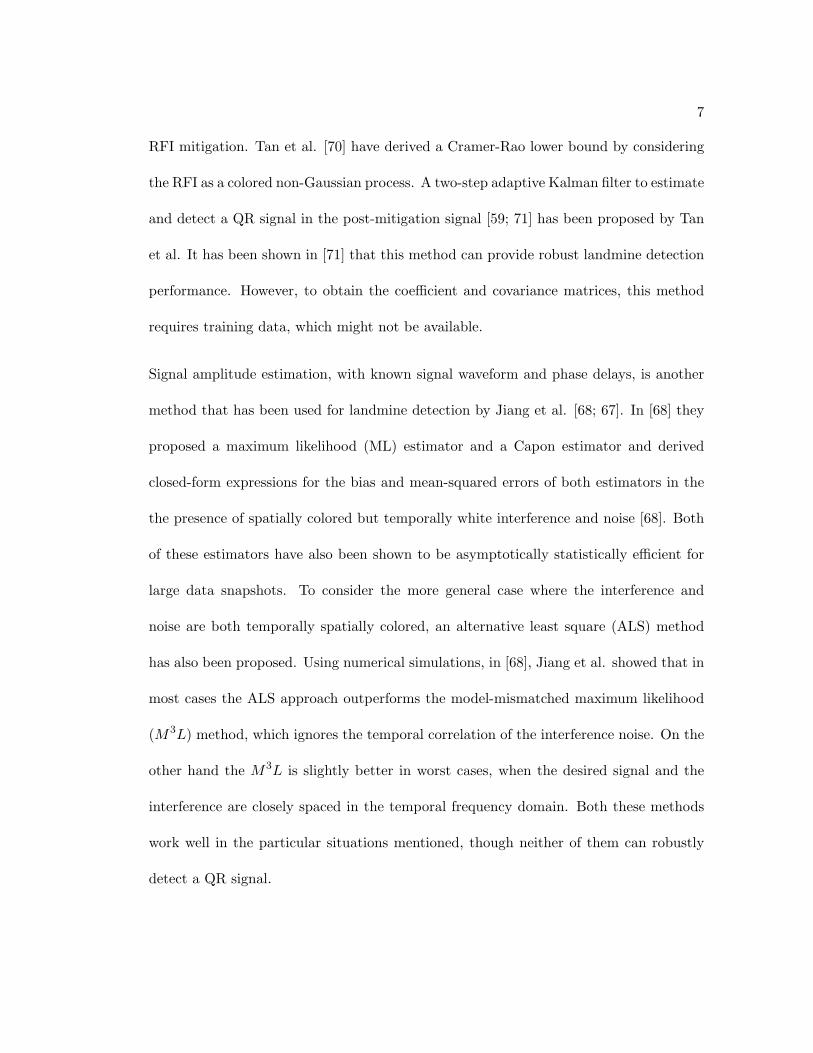
RFI mitigation. Tan et al. [70] have derived a Cramer-Rao lower bound by considering
the RFI as a colored non-Gaussian process. A two-step adaptive Kalman filter to estimate
and detect a QR signal in the post-mitigation signal [59; 71] has been proposed by Tan
et al. It has been shown in [71] that this method can provide robust landmine detection
performance. However, to obtain the coefficient and covariance matrices, this method
requires training data, which might not be available.
Signal amplitude estimation, with known signal waveform and phase delays, is another
method that has been used for landmine detection by Jiang et al. [68; 67]. In [68] they
proposed a maximum likelihood (ML) estimator and a Capon estimator and derived
closed-form expressions for the bias and mean-squared errors of both estimators in the
the presence of spatially colored but temporally white interference and noise [68]. Both
of these estimators have also been shown to be asymptotically statistically efficient for
large data snapshots. To consider the more general case where the interference and
noise are both temporally spatially colored, an alternative least square (ALS) method
has also been proposed. Using numerical simulations, in [68], Jiang et al. showed that in
most cases the ALS approach outperforms the model-mismatched maximum likelihood
(M3L) method, which ignores the temporal correlation of the interference noise. On the
other hand the M3L is slightly better in worst cases, when the desired signal and the
interference are closely spaced in the temporal frequency domain. Both these methods
work well in the particular situations mentioned, though neither of them can robustly
detect a QR signal.
8
Other QR signal detection algorithms have been studied by Stegna [55]. These include
the Bayesian method and the maximum entropy (ME) method. The Bayesian method
has been reported to be the most robust method against noise. However, it requires a pri-
ori information which may not be available. The ME method has been shown to degrade
rapidly as the SNR decreases and has been reported to be the most computationally
intensive among the three methods.
Jakobsson et al. used the characteristic of temperature dependency of the QR frequencies
to develop several methods for QR signal detection. Among these is a non-linear least
squares method, an approximate maximum likelihood detector (AML), and a frequency
selective AML detector [7; 8; 6].
In regards to using the matched filter as a possible detector, some only mentioned it is
a possible detector, if the exact QR signal was known, and did not evaluate its perfor-
mance. Others proposed using filters matched to signals other than QR signal. Tan [59]
and Garroway et al. [11] have proposed using the matched filter as a possible filter to
maximize SNR when the signal s is a deterministic one and the noise is white, though
they have not evaluated its performance. Tan has also developed a filter, the complex-
valued quadrature matched filter, using the generalized likelihood ratio test under the
assumption that the RFI noise is white after RFI mitigation and averaging [59]. This
filter is referred to as a matched filter, since it uses estimates of the QR signal’s param-
eter but is actually different than what is generally referred to as a matched filter. The
filter assumes perfect demodulation of the QR signal s, i.e. that the resonant frequency
9
is exactly known, and the magnitude and phase of the complex envelope of the QR sig-
nal are found using maximum likelihood estimates and knowledge of their distributions.
The resulting filter, after demodulation and RFI mitigation, demodulates the complex
envelope of the QR signals by assuming its frequency is where the FFT of the envelope
peaks. The signal is then segmented and the square magnitude is averaged and compared
to a threshold.
Others have proposed or used filters that are matched to signals other than the QR
signal to detect explosives. Goldman et al.[24] developed a method that sends an elec-
tromagnetic signal into the ground and receives a response. The response is processed to
generate an image and determine whether a mine is present. He states that the SNR ratio
can be improved by using a matched filter and then continues to state that the matched
filter response is unknown and the step will be skipped. Barrall et. al [23] worked on
a method to cancel extraneous signals by irradiating the target with a specific sequence
of electromagnetic pulses referred to as SLIME. QR signals of one phase are subtracted
from QR signals having the opposite phase, resulting in a cumulative echo signal and
simultaneously subtracting out the same-phase extraneous signal. He proposed using
a weighing factor when averaging the echoes to increase the SNR. That is due to the
fact that the SNR decreases with time after transmission of the excitation pulse. The
weighting factors are chosen so that the weighting assigned to the echoes corresponds
to the decay envelope of the echo signal. He refers to this as matched filter exponential
weighting; i.e. matched to an exponential function with a decay constant. Bulsara et.
al [10] designed a stochastic resonator signal detector to detect the presence of a QR
10
signal. A stochastic resonator comprises of a multistable nonlinear device for coupling
to an input signal and a control signal coupled to the multi-stable nonlinear device for
varying asymmetry among stable states of the multi-stable nonlinear device. The in-
teraction of the input signal with the control signal in the multistable nonlinear device
generates an output signal having an amplitude responsive to the input signal amplitude
and a frequency range that comprises harmonics from the product of the control signal
and the input signal. The matched filter is used to detect the presence of harmonics in
these frequencies.
1.3 Approach
Although all the previously mentioned methods contributed to the problem of robustly
detecting a QR signal in the presence of AM RFI’s, none were capable of completely
solving the problem. These methods have also not exploited the shape of the QR signal.
Even though the exact description of the QR signal is unknown, the general shape is.
This leads to the idea of matched filters and robust matched filters, which is the approach
proposed in this thesis.
The thesis first motivates the use of matched filters in QR detection by showing the im-
provements in detection rates when more information about the signal is used. Though,
to be able to evaluate and compare the performance of the matched filter to the generic
energy detector we assume that exact knowledge of the QR signal is attainable, an
assumption placed just for the sake of an elementary comparison. Receiver operating
characteristic (ROC) plots, a graphical plot of sensitivity vs specificity, are used as a
11
measure of comparison between the two detection algorithms. Theoretical calculations
of the distribution of these plots will be compared to simulation and experimental values
for both the energy detector and matched filter algorithms. Under the given assump-
tions, the matched filter outperforms the energy detector. The method of estimating
the QR signal and noise characteristics is then presented. These estimates are used to
obtain a filter closely matched to the QR signal, had one been present, and the noise
statistics. The method of designing matched filters robust over signal and noise sets is
then presented, whose ultimate aim is to gain robustness to variances in the QR signal.
The following chapter presents QR spectroscopy and the experimental procedure used.
This is followed by a chapter that will present the observed QR and noise signals. The
motivation behind using the matched filter as a detector is then presented in Chapter
4. This chapter is followed by an introduction of our approach of estimating a filter
matched to the QR signal present. This is followed by a chapter, that combines the
work from the former chapter with an approach to estimating the statistics of the noise
signal present, to design a filter matched to both the QR signal and the noise present.
The thesis then ends with a chapter that introduces a matched filter robust to a signal
and noise sets pair. This chapter only uses simulation data to analyze the performance
of robust filters for sets of QR signals with varying parameters. Though, the ultimate
goal is to design filters robust to uncertainties in the general shape of the QR signal
instead of uncertainties in the QR signal parameters.
12
Chapter 2
QR Spectroscopy
Although the focus of this thesis is on the signal processing algorithms of QR detection,
it is important to provide a brief overview of QR spectroscopy. This chapter starts
by introducing the physics behind the QR detection process. The chapter then moves
on to introducing the signals observed in QR. This is followed by an introduction of
the excitations pulses used in QR detection. Lastly, the QR detection procedure is
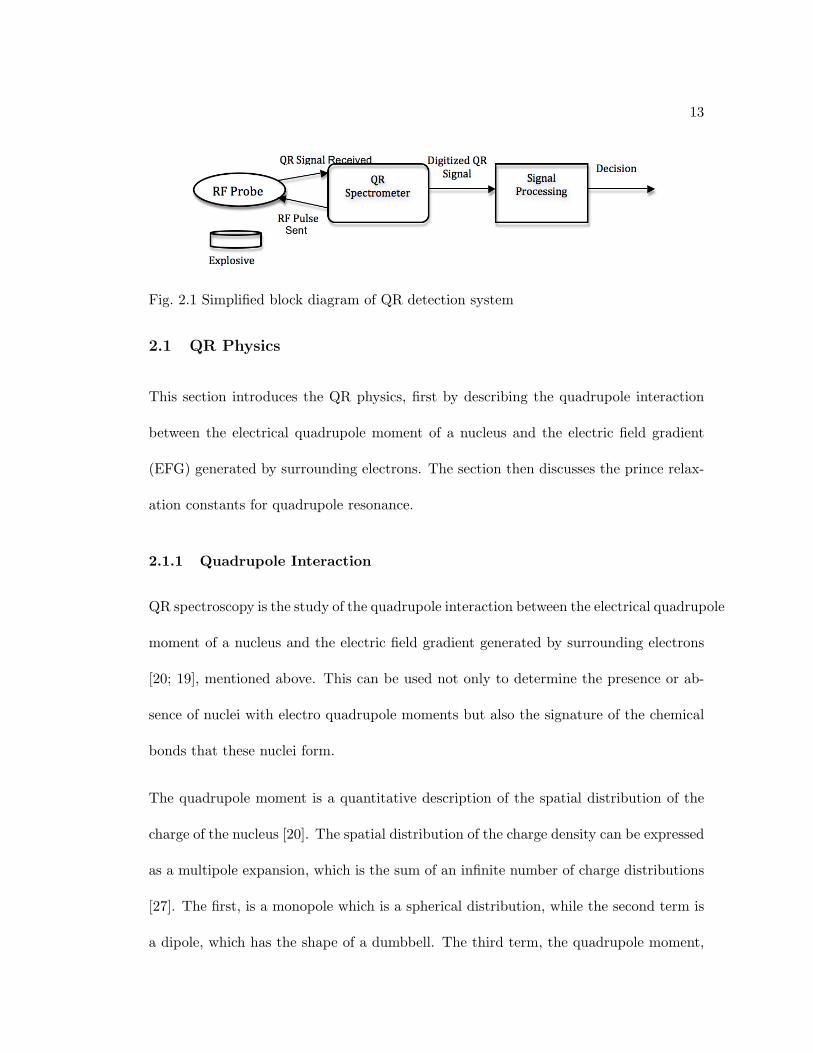
introduced. Figure 2.1 is a simplified block diagram of the QR detection system.
The idea behind QR detection is straightforward. Certain material, such as explosives,
contain nuclei that form a resonant system because of their interaction between their
electrical quadrupole moment and electrical field gradient. By applying a radio frequency
pulse, whose frequency matches this interaction energy, it is possible to perturb the sys-
tem. Once a system is perturbed, it prodcasts a signal at the same frequency whose
presence would reveal the presence of the explosive material. The QR spectrometer
shown sends an RF pulse or a series of RF pulses, of frequency matched to the material
of interest. The probe then receives a response that is passed to the QR spectrome-
ter. Briefly, the spectrometer digitizes and demodulates the received signal. A signal
processing algorithm is then applied to determine the presence of a QR signal.
13
Fig. 2.1 Simplified block diagram of QR detection system
2.1 QR Physics
This section introduces the QR physics, first by describing the quadrupole interaction
between the electrical quadrupole moment of a nucleus and the electric field gradient
(EFG) generated by surrounding electrons. The section then discusses the prince relax-
ation constants for quadrupole resonance.
2.1.1 Quadrupole Interaction
QR spectroscopy is the study of the quadrupole interaction between the electrical quadrupole
moment of a nucleus and the electric field gradient generated by surrounding electrons
[20; 19], mentioned above. This can be used not only to determine the presence or ab-
sence of nuclei with electro quadrupole moments but also the signature of the chemical
bonds that these nuclei form.
The quadrupole moment is a quantitative description of the spatial distribution of the
charge of the nucleus [20]. The spatial distribution of the charge density can be expressed
as a multipole expansion, which is the sum of an infinite number of charge distributions
[27]. The first, is a monopole which is a spherical distribution, while the second term is
a dipole, which has the shape of a dumbbell. The third term, the quadrupole moment,
14
can be viewed as two anti-parallel electric dipoles, hence the name quadrupole. Though
the only charge distribution of interest to us is the quadrupole moment. The electric
quadrupole moment is a tensor that can be described with a single parameter eQ, where
e is the magnitude of an electron’s charge and Q is a scalar parameter that measures
the departure of the electric charge distribution from the spherical symmetry. When the
nuclear charge density is spherical, then the electric quadrupole parameter eQ is zero.
This value is positive, when the nuclear charge density is elongated along an axis of
symmetry and the charge density is shaped like an ellipse. On the other hand when eQ
is negative, the charge distribution is flattened like a frisbee.
The other component needed for quadrupole interaction, the electric field gradient (EFG)
is determined by the charge distribution within the bonds that the nucleus forms with
other atoms. The components of the tensor EFG can be reduced to two, which are the
maximal electric field gradient (EFG), eq and the asymmetry parameter, η. A non-zero
EFG’s interaction with the monopole, dipole, or any higher odd moment of the multipole
expansion of the nuclear charge distribution results in a zero torque acting on the nuclei
[19]. On the other hand, the EFG’s interaction with the quadrupole moment and higher
order even moments result in a non-zero torque, but only the one with the quadrupole
moment results in a torque large enough to be observed. Therefore, the interaction of
the EFG gradient with the quadrupole moment is the only one of interest. This torque,
a result of the interaction, is proportional to e2Qq, the quadrupole coupling constant
[20]. Therefore, the nucleus has certain preferred orientations, and each orientation
corresponds to a separate electrostatic interaction energy [52].
15
The quadrupole nuclei also posses angular momentum, referred to as spin, S. This
angular momentum is a vector quantity that is quantized by the axioms of quantum
mechanics. The magnitude of the vector is related to the spin quantum number I, which
can be an integer or a half integer value greater than zero. The possible spin directions m,
are functions of I, the spin quantum number. The value of m can be any value between
-I to +I in increments of one [18]. For example an I = 1, leads to three possible values
of m [52], (-1, 0 and 1). Quantization of the nuclear spin also leads to the quantization
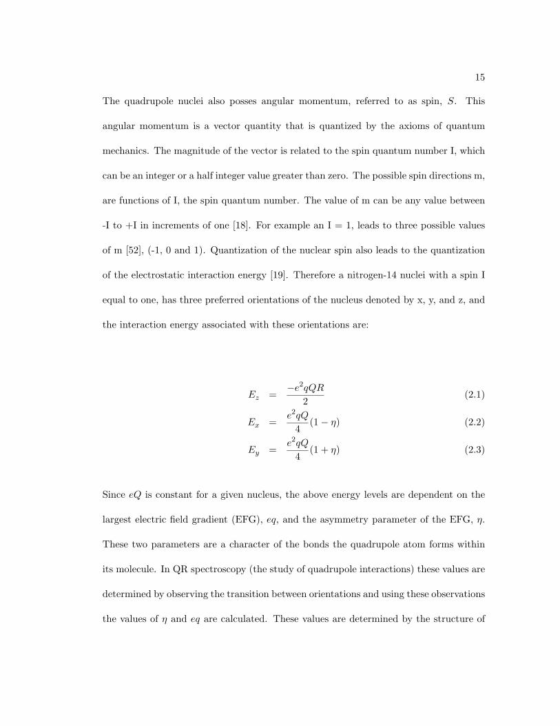
of the electrostatic interaction energy [19]. Therefore a nitrogen-14 nuclei with a spin I
equal to one, has three preferred orientations of the nucleus denoted by x, y, and z, and
the interaction energy associated with these orientations are:
Ez =−e2qQR
2(2.1)
Ex =e2qQ
4(1− η) (2.2)
Ey =e2qQ
4(1 + η) (2.3)
Since eQ is constant for a given nucleus, the above energy levels are dependent on the
largest electric field gradient (EFG), eq, and the asymmetry parameter of the EFG, η.
These two parameters are a character of the bonds the quadrupole atom forms within
its molecule. In QR spectroscopy (the study of quadrupole interactions) these values are
determined by observing the transition between orientations and using these observations
the values of η and eq are calculated. These values are determined by the structure of
16
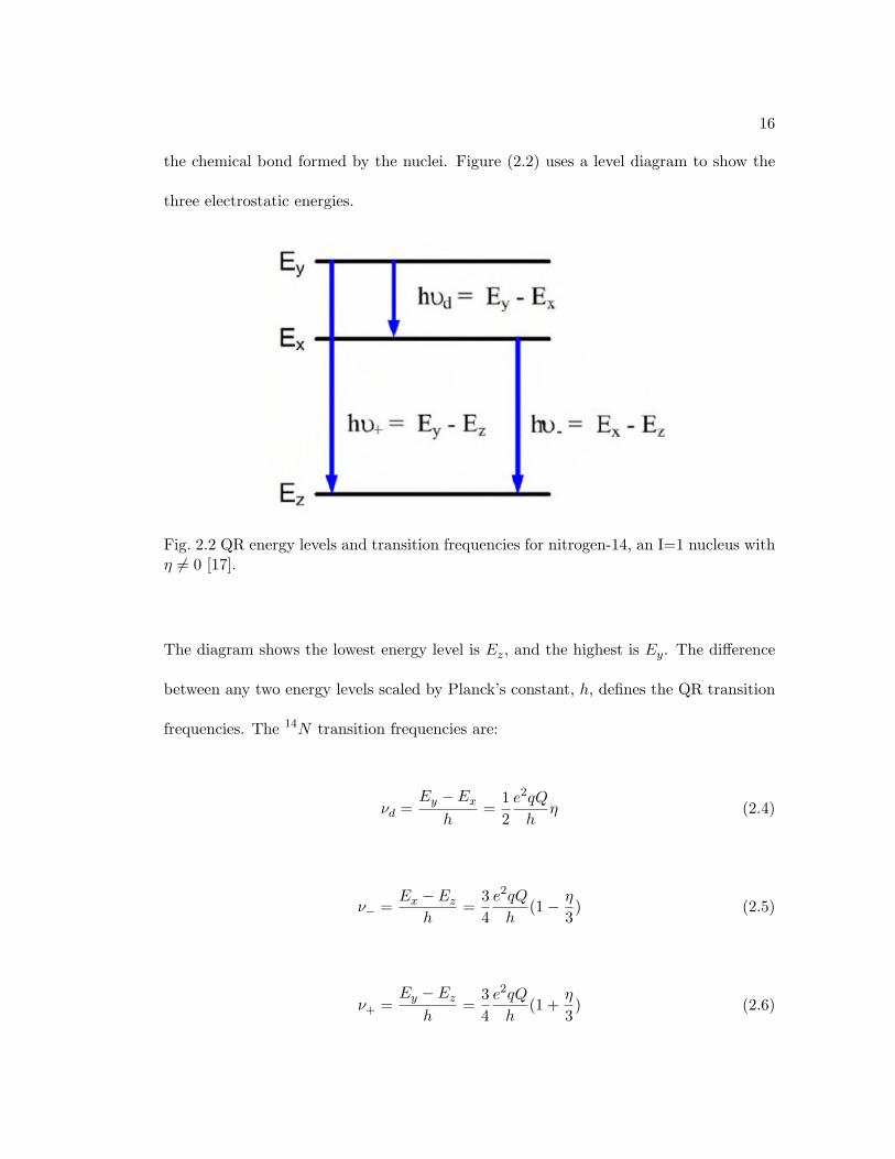
the chemical bond formed by the nuclei. Figure (2.2) uses a level diagram to show the
three electrostatic energies.
Fig. 2.2 QR energy levels and transition frequencies for nitrogen-14, an I=1 nucleus withη 6= 0 [17].
The diagram shows the lowest energy level is Ez, and the highest is Ey. The difference
between any two energy levels scaled by Planck’s constant, h, defines the QR transition
frequencies. The 14N transition frequencies are:
νd =Ey − Ex
h=
12e2qQ
hη (2.4)
ν− =Ex − Ez
h=
34e2qQ
h(1− η
3) (2.5)
ν+ =Ey − Ez
h=
34e2qQ
h(1 +
η
3) (2.6)
17
As stated earlier, when the asymmetry parameter, η is zero, the energy levels Ex and
Ey are degenerate since they represent the same energy [52]. Figure (2.2) displays the
three transition frequencies with respect to their energy levels.
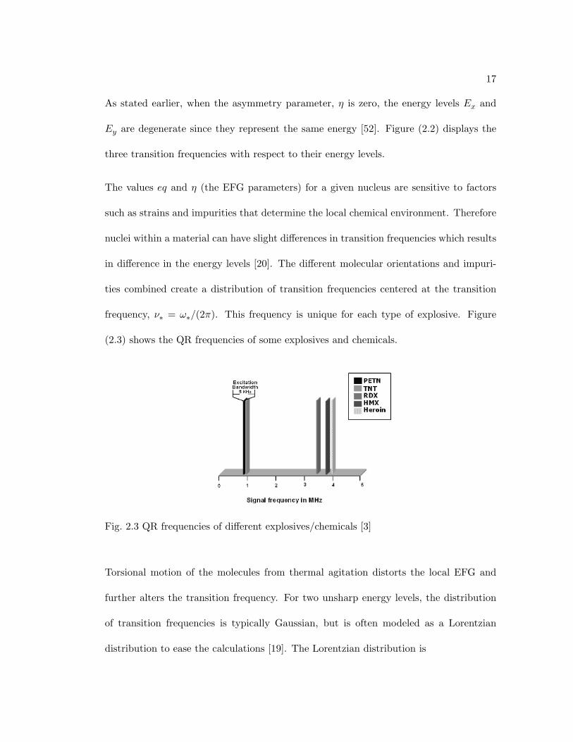
The values eq and η (the EFG parameters) for a given nucleus are sensitive to factors
such as strains and impurities that determine the local chemical environment. Therefore
nuclei within a material can have slight differences in transition frequencies which results
in difference in the energy levels [20]. The different molecular orientations and impuri-
ties combined create a distribution of transition frequencies centered at the transition
frequency, ν∗ = ω∗/(2π). This frequency is unique for each type of explosive. Figure
(2.3) shows the QR frequencies of some explosives and chemicals.
Fig. 2.3 QR frequencies of different explosives/chemicals [3]
Torsional motion of the molecules from thermal agitation distorts the local EFG and
further alters the transition frequency. For two unsharp energy levels, the distribution
of transition frequencies is typically Gaussian, but is often modeled as a Lorentzian
distribution to ease the calculations [19]. The Lorentzian distribution is
18
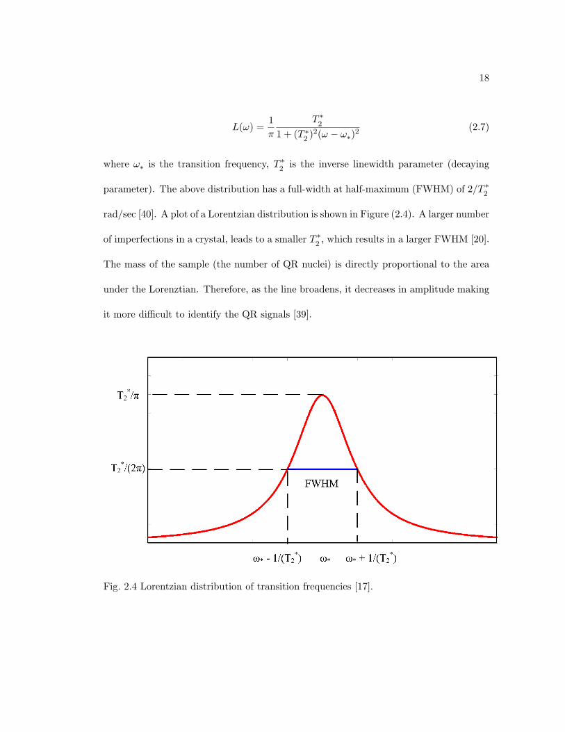
L(ω) =1π
T ∗2
1 + (T ∗2
)2(ω − ω∗)2 (2.7)
where ω∗ is the transition frequency, T ∗2
is the inverse linewidth parameter (decaying
parameter). The above distribution has a full-width at half-maximum (FWHM) of 2/T ∗2
rad/sec [40]. A plot of a Lorentzian distribution is shown in Figure (2.4). A larger number
of imperfections in a crystal, leads to a smaller T ∗2
, which results in a larger FWHM [20].
The mass of the sample (the number of QR nuclei) is directly proportional to the area
under the Lorenztian. Therefore, as the line broadens, it decreases in amplitude making
it more difficult to identify the QR signals [39].
Fig. 2.4 Lorentzian distribution of transition frequencies [17].
19
The following subsection discusses the relaxation mechanisms of QR and time constants
associated with QR spectroscopy.
2.1.2 Relaxation Mechanisms
The principle relaxation parameters for QR are the spin-lattice and spin-spin relaxation
constants [38]. The spin-lattice relaxation time constant, T1, describes the length of
time needed for the RF energy absorbed by the nuclei (from pulsing) to be dissipated
by the nuclei to the surrounding lattice. The lattice is the general name for all other
degrees of freedom of the system besides spin orientation such as translational motion of
the molecules [50]. This relaxation time constant, T1, is physically proportional to the
time it takes the nuclei returning to their thermal equilibrium orientation. The spin-spin
relaxation time constant, T2eff , describes how the energy is exchanged among nuclei
through the interaction of their magnetic dipole moments. This interaction produces a
perturbation in the transition frequencies that causes the magnetic moments of precessing
nuclei to interfere destructively. Unlike the T ∗2
decay constant, which is the result of a
time-independent disturbance in transition frequencies, the T2eff relaxation is caused by
random fluctuations. Since the latter loss can not be recovered, it is termed a relaxation
process [50]. It can be shown that T1 > T2eff > T ∗2
.
For example if a sample is in thermal equilibrium and is pulsed the largest possible QR
signals is produced and after a few T2eff time constants the observed signal will vanish
due to destructive interference among the processing nuclei. Therefore, to obtain the
maximum response from a sequence of RF pulses one must wait a minimum of three
T1 constants for thermal equilibrium magnetization to be restored. Reducing the pulse
20
spacing causes the amplitude of QR signals from successive pulses to decrease. Therefore,
the pulse sequences used will wait at least three T1 between pulses. The following section
introduces the observed signals in QR detection.
2.2 Observed Signals
Two commonly observed signals in QR detection are the free induction decays (FIDs)
and the spin echoes. The two kinds of signals are described as follows [45; 52; 53; 51; 44].
• Free Induction Decays: The FID is a decaying signal caused by the interaction
between the oscillating magnetic field of the applied RF pulse with the magnetic
moment of the quadrupolar nucleus. This signal is observed immediately following
the applied RF pulse. Due to the fast decay of this signal and the ringing after
applying the RF pulse, this signal is hardly used for QR detection.
• Spin Echoes: After applying an RF pulse, spins become dephased causing the
QR signal to diminish [45]. Using appropriate pulse sequences, these spins can be
momentarily placed back in phase to generate useful spin echoes. These echoes can
be observed for a longer period of time than the FIDs, which makes them useful
for QR detection.
2.3 RF Excitation Pulse Sequences
The design of the RF pulse excitation sequence is a vital step in the process of obtaining
a useful QR signal. Though the QR signal is small in amplitude, the SNR ratio can be
improved by coherently adding the individual echoes acquired from each pulse. This is
21
led to the study and development of multi-pulse sequences in QR applications, which
can drastically improve the detection capability of the QR signal. The most commonly
used multi-pulse sequences represent some form of the spin-lock spin echo (SLSE) or the
strong off-resonant comb (SORC).
The spin-lock spin echo sequence, introduced in the 1970’s, generates a sequence of de-
caying spin-echoes. These echoes appear in between the rephasing pulses of the sequences
and decay in an approximately exponential manner. The strong off-resonant comb pulse
sequence is a steady state free procession, which was first introduced in the early 1980s
[47], composed of a sequence of equally spaced off-resonant pulses. This SORC sequence
generates a sequence of stable non-decaying spin-echoes [15], located at the rephasing
pulses. The spin echoes from both these sequences can be coherently added to improve
the SNR, [15]. One of the advantages of using the SORC sequence is that the sequences
last for as long as the rephasing pulse is applied, unlike SLSE. Unfortunately the SORC
sequence may not be used with all explosives, an example of such an explosive is TNT.
Another advantage of using the SORC sequence is that the amplitude of the generated
echoes are comparable to the free induction decay signal. The signal processing algo-
rithms discussed in this thesis are applicable independently of which pulse sequence is
used, though the type of pulse sequence used will affect the decay factor of the echoes.
The energy or equivalently the product of the amplitude and width of the RF pulses
determine the angle in which the nucleus is rotated. The frequency of the RF pulses
must match the energy difference between any two interaction energy levels. The next
section provides a brief overview of the QR detection procedure.
22
2.4 QR Detection Procedure
The process of detecting a QR signal can be summarized in the following steps:
• A series of RF magnetic pulses, known as excitation pulses, are generated and
emitted by a transmitter.
• Each pulse, from the series of pulses, perturbs the alignment of the nitrogen nuclei
within the material.
• During the inter-pulse interval, the precessing nuclei relax back to the their original
state. This motion of magnetic moment of the nuclei induces a voltage across the
probe coil, which is the QR response
• The QR response is received by the receiver and after passing through an amplifier
and digital converter, the received signal is sent to a computer based processor.
• The processor then analyzes the received signal, based on a specific algorithm
(such the one developed in this thesis), and a decision on whether the sought after
explosive is present is made.
To better understand the digitized received signals at the output of the QR spectrometer
(Schiano [48]), we need to provide a more detailed description of the spectrometer. A
block diagram describing the QR spectrometer is shown in Figure 2.5. During the receiv-
ing mode, the spectrometer uses a double heterodyne system that includes a quadrature
phase detector to demodulate the QR response to a lower frequency so that it can be
digitized using an A/D converter. The frequency of the PTS D310 is set to ωr+10 MHz,
23
where ωr = ω∗+ω0, ω∗ is the QR transition frequency (or the spectrometer frequency we
are searching at ωs) and ω0 is the desired receiver offset frequency. The signal induced
across the probe is first amplified and then heterodyned with the PTS D310 output
signal. The output of the first heterodyne is then ran through a bandpass filter at 10
MHz resulting in signal whose spectra is centered at 10 MHz +ω0. This signal is het-
erodyned a second time in a quadrature phase detector at 10 MHz to produce in-phase
and quadrature signals whose spectra are approximately centered at ω0.
The signal spectra are not exactly centered at the ω0, since the frequency of the PTS
D310 is hardly ever set exactly to ωr + 10 MHz due to uncertainty in the QR transition
frequency, ω∗. The QR transition frequency of a material is temperature sensitive and
in some cases more sensitive than others. For example, the explosive RDX varies by
approximately 0.45 kHz/◦C [32], while piperazine is highly insensitive to changes in
temperature which is why it was used in collecting experimental data. The two signals,
the in-phase and quadrature, are then low passed by a filter with a cutoff frequency
of 20 kHz. They are then digitized and combined within the computer to produce the
complex-valued signal.
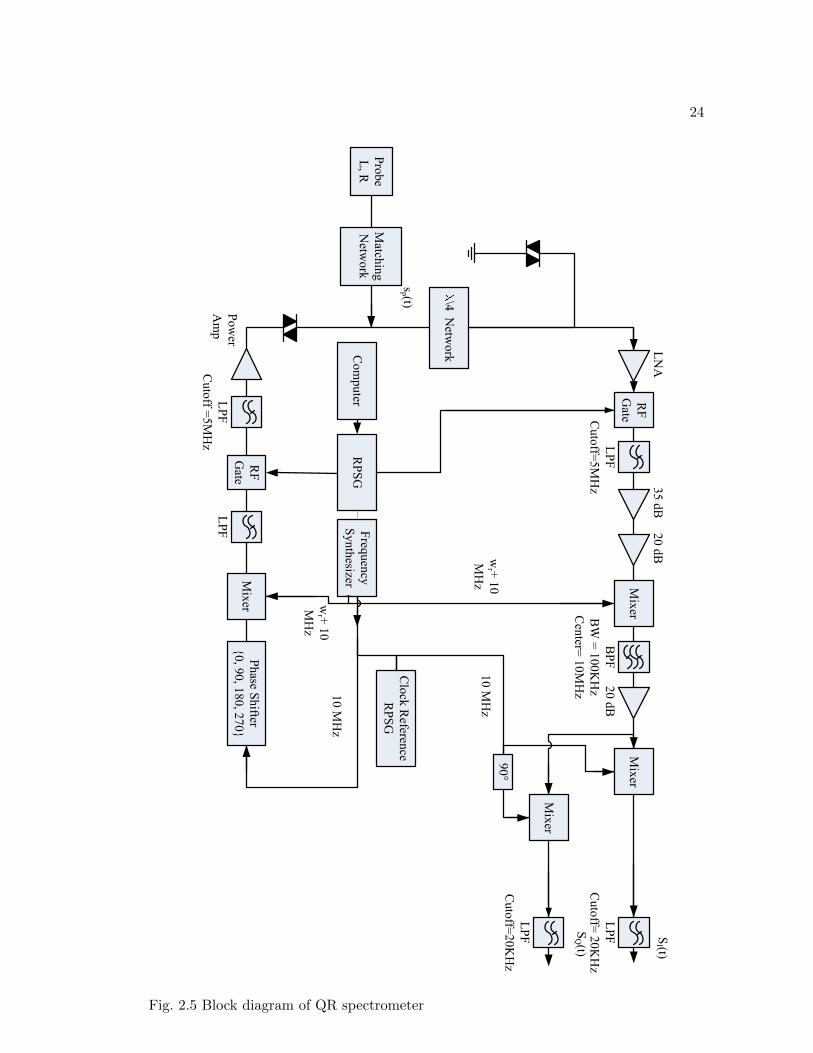
24
LP
F
Cu
toff =
5M
Hz
RF
Gate
LP
F
Mix
erP
hase S
hifter
{0, 9
0, 1
80, 2
70}
20 d
B
10
MH
z
\4 N
etwo
rk
35 d
B
LP
F
Cu
toff=
5M
Hz
RF
Gate
20 d
B
Mix
er
BP
F
BW
= 1
00
KH
z
Cen
ter= 1
0M
Hz
LN
A
Match
ing
Netw
ork
Pro
be
L, R
Mix
er
Mix
er
LP
F
Cu
toff=
20
KH
z
LP
F
Cu
toff=
20
KH
z
SI (t)
90°
Freq
uen
cy
Synth
esizerR
PS
GC
om
pu
ter
Pow
er
Am
p
Clo
ck R
eference
RP
SG
SQ(t)
sp (t)
wr +
10
MH
z
wr +
10
MH
z
10
MH
z
Fig. 2.5 Block diagram of QR spectrometer
25
Chapter 3
Challenges, Signal Characteristics and Data Generation
This chapter discusses the challenges faced in QR detection and provides a description
of the QR and corrupting noise signals.
3.1 Challenges
There are several challenges one faces in QR detection. Some are the result of uncer-
tainty in the QR signal, while others are due to external and internal radio frequency
interferences. Some of these challenges are discussed in the following subsections.
3.1.1 Challenges Due to Uncertainty QR Signal
In an ideal case, with no interferences, a spin echo received in between pulses by the coil
would resemble the signal shown in the top part of Figure (3.1), which is a sinusoidal
signal that exponentially decays about the center.
Depending on the spatial distribution of the magnetic field across your sample, this
signal can at times be more gaussian shaped than exponentially decaying about the
center, which brings in uncertainty in the general shape of the signal. It may also
contain more than a single frequency, depending on the temperature and strains of the
explosive material. Explosive material within a bomb is required to have a uniform
temperature to obtain a signal with a very narrow bandwidth. All these reasons cause
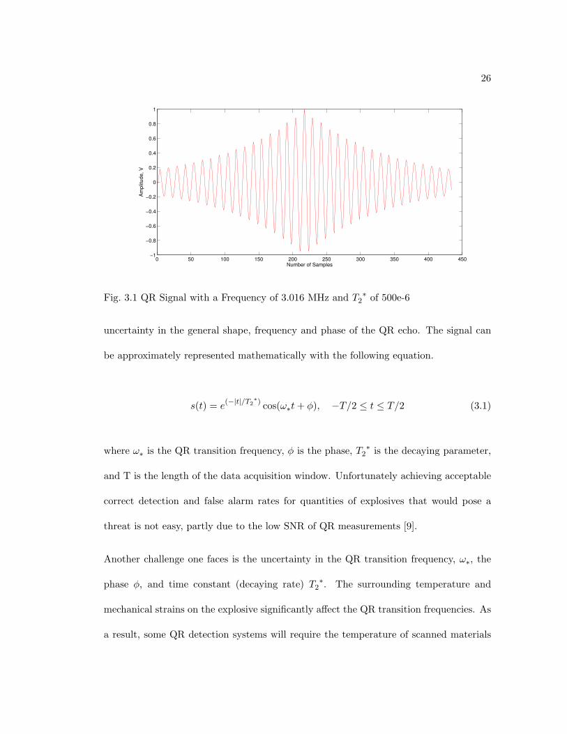
26
0 50 100 150 200 250 300 350 400 450−1
−0.8
−0.6
−0.4
−0.2
0
0.2
0.4
0.6
0.8
1
Am
plit
ude, V
Number of Samples
Fig. 3.1 QR Signal with a Frequency of 3.016 MHz and T2∗ of 500e-6
uncertainty in the general shape, frequency and phase of the QR echo. The signal can
be approximately represented mathematically with the following equation.
s(t) = e(−|t|/T2∗) cos(ω∗t+ φ), −T/2 ≤ t ≤ T/2 (3.1)
where ω∗ is the QR transition frequency, φ is the phase, T2∗ is the decaying parameter,
and T is the length of the data acquisition window. Unfortunately achieving acceptable
correct detection and false alarm rates for quantities of explosives that would pose a
threat is not easy, partly due to the low SNR of QR measurements [9].
Another challenge one faces is the uncertainty in the QR transition frequency, ω∗, the
phase φ, and time constant (decaying rate) T2∗. The surrounding temperature and
mechanical strains on the explosive significantly affect the QR transition frequencies. As
a result, some QR detection systems will require the temperature of scanned materials
27
to lie within a specified range. Due to this, the transition frequency, ω∗, in Equation
(3.1) is only known to fall within an upper and lower bound as follows,
ωlb ≤ ω∗ ≤ ωub (3.2)
The values ωlb = ωs − RBW /2 and ωub = ωs + RBW /2 are the lower and upper bound
frequency values respectively, and are dependent upon the known values ωs, spectrometer
frequency, and RBW , the bandwidth of the receiver, which is 20 kHz in our experimental
setup. The bandwidth of the receiver, RBW , varies with the type of coil used.
Uncertainty in the phase of the QR signal poses yet another challenge in QR detection.
The phase in Equation (3.1) is only known to fall within upper and lower bound as
follows,
−π ≤ ω∗ ≤ π (3.3)
Yet another challenge is uncertainty in the explosives time constant, T2∗. The quality
of the explosive highly affects the time constant, T2∗, of the QR response, for example
a fixed quantity of plastic explosive manufactured in an explosive manufacturing plant
will have a different time constant than the same quantity of explosive manufactured in
less artisanal methods. As a result the time constant, T2∗, is only known to fall within
an upper and lower bound as follows
T2∗lb ≤ T2
∗ ≤ T2∗ub. (3.4)
28
Presented next, are the challenges imposed from noise signals.
3.1.2 Challenges Due to External and Internal RFI Signals
Interferences from external RF sources pose another challenge when trying to detect a
QR signal. Since the frequency of the QR signal is low, between 0.5 and 6 MHz [44],
they are unavoidably corrupted by external radio frequency interferences, RFIs, located
in their frequency band. AM stations and ignition noises can trigger false alarms when
attempting to detect a QR signal. To overcome the challenge posed by external RFIs
it is essential for one to understand the source of these interferences. Of main interest
to us are RFIs from AM broadcast stations, since they are a major contributor to the
external interferences.
AM station frequency bands can be classified into three categories: long wave, medium
wave and short wave. Two of which, the medium and short wave, overlap with the
frequencies of QR signals from certain materials. The medium band is the one used
for commercial broadcasting and falls between 520 kHz and 1, 610 kHz, with channel
spacing of 10 kHz in the U.S. and 9 kHz elsewhere. The third one, is the short wave
band and is used for audio services intended to be heard at great distances from the
transmitting station, and falls in the range of 1.711 MHz −30 MHz with channel spacing
of 5 kHz. Among those three bands fall clear channel stations, which can be heard across
the country due to their large transmitting power.
One particular clear channel station to be concerned about is the Chicago based WLS
channel, which broadcasts at 890 kHz, the exact QR frequency of PETN. This is a
29
problem for QR detection. Another example where the QR frequency of the material
falls within the AM broadcast band is the frequency of the explosive TNT, which is
at 842 kHz at normal room temperature [9]. This frequency falls within the AM radio
frequency band and as a result the performance QR signal detection at that frequency
is seriously degraded.
Therefore to detect these weak QR signals, it becomes essential to mitigate the RFIs
using methods similar to [9; 45; 68; 59]. A single corrupting AM signal can be described
using the following mathematical equation.
AM i(t) = A(1 +m(t)) cos(ωct+ φi) 0 ≤ t ≤ T (3.5)
where φi is a random phase shift between π and −π that is variable and T is the period
of the QR signal. The frequency of the carrier is ωc and the message being modulated
is m(t).
The center of Figure (3.2) shows an AM signal, while bottom of Figure (3.2) shows a QR
signal corrupted by an AM signal with an SNR ratio of 0.25 or -12 dB. The resemblance
between the AM signal and the corrupted QR signal is obvious, even with this high SNR,
when compared to SNR values observed without noise shielding. Shielding can minimize
external RF interferences, though there exist situations where shielding is not applicable.
One particular example is the detection of anti-tank land mines. This makes the detection
of these mines a particular difficult task in the evening, when worldwide broadcasts
interfere with the detection process. Other sources of RF interference are internal ones,
from sources within the search volume. The excitation of a QR response requires the
30
application of a pulsed RF magnetic field within the search volume. Currents induced
within conductive materials located in the search volume, cause decaying magnetic fields
that lead to unacceptable false alarm rates.
0 50 100 150 200 250 300 350 400 450−1
0
1
Am
plit
ude, V
0 50 100 150 200 250 300 350 400 450−5
0
5
Am
plit
ude, V
0 50 100 150 200 250 300 350 400 450−5
0
5
Am
plit
ude, V
Number of Samples
Fig. 3.2 Comparison of QR+AM and QR: (Top) QR Signal with a Frequency of 3.016MHz and T2
∗ of 500e-6 (Center) AM Signal with Carrier Frequency of 3.016 MHz (Bot-tom) QR plus AM Signal, SNR = -12 dB
Another concern is the ringing produced by the search coil and the remaining hardware
[9; 45]. The coil can not immediately obtain the QR signal although the exciting pulse
has ended [45]. Performing phase cycling on the pulse sequence is an efficient way to
reduce the ringing problem [9; 58; 45]. Another method is using an active Q-spoiling
system which allows the probes natural response to relax rapidly following the excitation
pulse to permit detection of the QR response, [42]. Other RFI mitigation methods are
discussed in the following section.
31
3.2 RFI Mitigation Methods
Signal averaging, which is discussed in the following section, is another efficient method
used to tackle the major challenge of low SNR ratio [9; 15]. For uncorrelated noise, the
SNR increases by the square root of the number of averaged QR signals [15]. However
this method is ineffective in the presence of correlated noise or interferences such as AM
noise, [15]. Optimizing the search coil design can also improve the SNR ratio and hence
improve the probability of detecting a QR signal. Several design issues and ways to
improve the design have been addressed by Suits et al. [13; 57; 12; 14].
The SNR can also be enhanced by reducing the RFIs. Both active and passive strategies
in the hardware design have been considered [9]. The Naval Research Laboratory (NRL)
designed gradiometer coil, which measures the difference in magnetic flux [13]. This is
considered a passive approach and they claim that the gradiometer coil can reduce the
far field magnetic interference by 30 dB [9]. However, the coil may reduce the QR signal
at the same time [13], which in turn would reduce the probability of detection. In [45],
asymmetric gradiometers have been proposed to partly solve the QR signal loss problem
[45].
An efficient QR coil (used as the main antenna) and a set of external remote antennas
(used as reference antennas) have been developed by QM to reduce RFIs [9]. The goal of
the main antenna is to receive both RFIs and a QR signal, while the reference antennas
only receive RFIs [9]. The RFI”s from the reference antennas are used to mitigate the
RFIs at the main antenna. This method’s main disadvantage is that it requires high
dynamic range and an accurate balance of antennas. The approach proposed in this
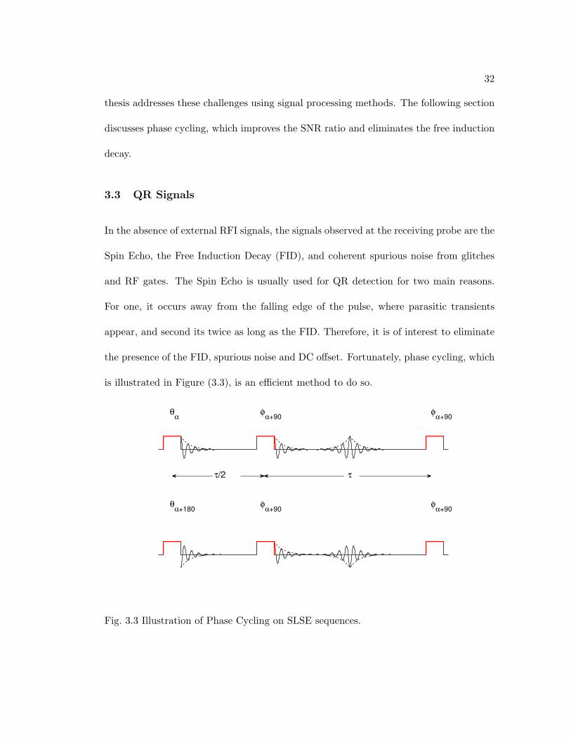
32
thesis addresses these challenges using signal processing methods. The following section
discusses phase cycling, which improves the SNR ratio and eliminates the free induction
decay.
3.3 QR Signals
In the absence of external RFI signals, the signals observed at the receiving probe are the
Spin Echo, the Free Induction Decay (FID), and coherent spurious noise from glitches
and RF gates. The Spin Echo is usually used for QR detection for two main reasons.
For one, it occurs away from the falling edge of the pulse, where parasitic transients
appear, and second its twice as long as the FID. Therefore, it is of interest to eliminate
the presence of the FID, spurious noise and DC offset. Fortunately, phase cycling, which
is illustrated in Figure (3.3), is an efficient method to do so.
τ/2 τ
θα
θα+180
φα+90
φα+90
φα+90
φα+90
Fig. 3.3 Illustration of Phase Cycling on SLSE sequences.
33
When the phase of the first lock pulse is changed by 180 degrees, the phase of the echoes
are changed accordingly while the phase of the FID and noise are not. Performing
this procedure on successive pulse sequences is called phase cycling. The sequence of
echoes, resulting from the difference of the two sequences, are then averaged to obtain a
single echo. In the case of uncorrelated noise, the root-mean-squared amplitude of the
noise component in the composite signal decreases with the square-root of the number
of averages, at the expense of increasing detection time [21].
As was discussed in Section 2.3, there are several different excitation pulses used for QR
detection. The two most commonly used multi-pulse sequences are the spin-lock spin
echo (SLSE) and the strong off-resonanct comb(SORC). Other pulse sequences represent
some form of the SLSE or SORC sequences. The type of pulse sequence used affects the
single averaged echo resulting from a pair of phase cycled pulse sequences, as will be
shown in the mathematical description of the averaged echo.
As was mentioned in the previous section, in an ideal case, with no interferences, an echo
received at the coil can be approximated as,
sp(t) = e(−|t|/T2∗) cos(ω∗t+ φ), (3.6)
which is a single frequency spin-echo with a Lorentzian distribution in the absence of
noise. The parameter T2∗ defines the decaying rate of QR signal, while ω∗ is the QR
transition frequency, and both are material specific. To use the above mathematical
34
form of the QR signal, we place the following assumption on the received QR signal
throughout this thesis.
Assumption 1. The full width at half maximum, FWHM1, of sp(t) in equation (3.6) is
sufficiently small compared to the 3 dB bandwidth of the probe, the bandpass filter and
the low pass filter in the quadrature phase detector.
When the signal in Equation (3.6) is passed through the QR spectrometer, if Assumption
1 holds, the output signals are the following discrete time signals
sI [k] = Ae(−|−T/2+k∆|/T2∗) cos (ωbb(−T/2 + k∆) + φbb) (3.7)
sQ[k] = Ae(−|−T/2+k∆|/T2∗) sin (ωbb(−T/2 + k∆) + φbb) (3.8)
for k = 0, 1, . . . , Ns−1, where ωbb is the base-band frequency, φbb is the base-band phase,
T is the length of the data acquisition window, Ns is the number of discrete samples,
and ∆ = T/(Ns − 1) is the time increment in between sample points. We will assume
in this thesis that the base-band frequency, phase and decaying parameters are the only
unknowns in the QR’s signal description. The above two signals when combined form
the complex-valued digital signal,
sb[k] = sI [k] + jsQ[k] k = 0, 1, . . . , Ns − 1 (3.9)
= Ae(−|−T/2+k∆|/T2∗)e(jωbb(−T/2+k∆)+φbb) k = 0, 1, . . . , Ns − 1
1The full width at half maximum of a signal is the width of the frequency range where lessthan the half the signal’s power is attenuated, i.e. the power is at least half the maximum.
35
Although the output of the spectrometer is complex, the algorithms discussed in this
thesis will be compared while only exploiting the real part (3.7). Phase cycling and
averaging the real part from a pair of pulse sequences would be the next step for the
detection algorithms discussed in this work. Depending on the pulse sequence used in
generating the QR signals, one can experience decay across pulse echoes (SLSE). We will
assume that the averaged QR signal is a result of the following assumption.
Assumption 2. The ith QR echo of pulse sequence j decays with a factor of e−(i−1)τ/T2eff ,
where τ is the width of an echo and T2eff is a constant that is material dependent. This
constant describes how energy is exchanged among nuclei through the interaction of their
magnetic dipole moments. The interaction causes the magnetic moment of processing
nuclei to interfere destructively, which leads to a decay in the echoes [38]. When using a
SORC pulse sequence the value of T2eff is considered infinite (i.e. no decay). To simplify
the data simulation and calculations (Chapter 4) we assume no decay of echoes across
sequences for both SLSE and SORC sequences (the time in-between pulse sequences is
greater than 3T1, nuclei almost at thermal equilibrium), although the results can be ex-
tended to incorporate any decay. In other words the ith echo from the jth sequence will
have the same amplitude as the ith echo from the kth sequence.
Under Assumption 2, the real part of the averaged phase cycled QR echo, from a pair of
pulse sequences of Ne echoes each, can be represented as
spc[k] = β ∗Ae(−|−T/2+k∆|/T2∗) cos (ωbb(−T/2 + k∆) + φbb). (3.10)
36
for k = 0, 1, . . . , Ns − 1, where β is defined as
β =
Ne∑i=1
e−(i−1)τ/T2eff
Ne. (3.11)
When using the SORC sequence, which results in non-decaying echoes, the decaying
factor β is one. The thesis first evaluates and compares the performance of the energy
detector and matched filter under the assumption that the QR signal is exactly known in
Chapter 4. The thesis then moves on to evaluating and comparing the proposed batch
matched filter algorithm to the energy detector without this assumption in Chapter
5. Before comparing the two detection algorithms, a description of the observed noise
signals is presented next.
3.4 Noise Characteristics
The noise characteristic discussed in this thesis is a superposition of thermal and external
RF interference from AM signals. Due to its simplicity, thermal noise is discussed first
followed by AM signals.
3.4.1 Thermal Noise
Thermal noise received at the probe is processed by the QR spectrometer in the same
way a QR signal would be. A thermal noise signal at the output of the QR spectrometer
may be represented as,
nbi [k] = nIi [k] + jnQi [k] k = 0, 1, . . . , Ns − 1, (3.12)
37
where the nIi [k] and nQi [k] are filtered white gaussian random variables with a dis-
tribution, N(0, σ2tn
). Filtering the thermal noise correlates the noise samples, and the
samples can no longer be considered as white gaussian random variables. Phase cycling
and averaging the real part from a pair of pulse sequences leads to the following signal,
npc[k] =1
2Ne
Ne∑i=1
[nI [ζ(k, i)]− nI [ζ(k, i) + τd]] k = 0, 1, . . . , Ns − 1, (3.13)
where ζ(k, i) = k∆ + (i− 1)τ and τd is the time delay between the pulse sequences used
in phase cycling. The averaged phase cycled signal npc[k] for each k is the average of
2Ne noise samples.
3.4.2 AM Signals
Interferences from external RF sources pose a bigger threat, compared to internal RF
interferences, when trying to detect a QR signal. Since the frequency of the QR signal is
low (0.5 - 6 MHz [44]), they are unavoidably corrupted by external RFI sources located
in their frequency band. Of main interest to us are RFIs from AM broadcast stations,
since they are a major contributor to the external interferences.
A corrupting AM signal is represented in Equation (3.5). This AM signal is processed
by the QR spectrometer in the same way a QR signal is. Therefore, an AM signal at
the output of the spectrometer can be represented as,
ηIi [k] = Aηi(1 +mi[k∆]) cos (∆ωAMk∆ + φ) (3.14)
38
ηQi [k] = Aηi(1 +mi[k∆]) sin (∆ωAMk∆ + φ) (3.15)
for k = 0, 1, . . . , Ns− 1, where ∆ωAM is the frequency of the AM signal after demodula-
tion, m[.] is the broadcasted message, and φ is an unknown random phase shift between
π and −π. Equations (3.14) and (3.15) are combined to form the following composite
complex signal,
ηbi[k] = Aηi(1 +mi[k])e(j∆ωAM (k∆)+φ) k = 0, 1, . . . , Ns − 1. (3.16)
Again, even though the output of the QR spectrometer is complex, we will only be
utilizing the real part, the output of one channel. Phase cycling and averaging the real
part from a pair of pulse sequences, of Ne echoes each, would result in the following AM
signal,
ηpc[k] =Aη2Ne
Ne∑i=1
[(1 +m[ζ(k, i)]) cos (∆ωAM (ζ(k, i)) + φ)− (3.17)
(1 +m[ζ(k, i) + τd]) cos (∆ωAM (ζ(k, i) + τd) + φ)]
for k = 0, 1, . . . , Ns − 1, where ζ(k, i) = k∆ + (i− 1)τ and τd is the time delay between
the pulse sequences used in phase cycling.
3.5 Averaged Nm Trials
After Nm phase cycled trials are repeated, the Nm signals can be be averaged into
one signal, which is the approach taken when using the energy detector to detect the
39
presence of a QR signal. The averaged, uncorrupted QR signal, corrupting AM signal
and corrupting thermal noise signal have the form shown in Equations (3.18), (3.19) and
(3.20) respectively.
savg[k] =Nm−1∑i=0
spci [k]/Nm (3.18)
ηavg[k] =Nm−1∑i=0
ηpci [k]/Nm (3.19)
navg[k] =Nm−1∑i=0
npci [k]/Nm (3.20)
for k = 0, 1, . . . , Ns − 1, where Ns is the number of samples per trial and the index i
represents trial i + 1. The signals spci [k], ηpci [k] and npci [k] represent the phase cycled
signals and have the mathematical form shown in Equations (3.10), (3.17) and (3.13).
3.6 Aggregating Nm Trials
Instead of averaging the repeated Nm phase cycled trials, we can form an aggregated
discretized signal by stacking the Nm signals in time. This approach is used when using a
matched filter based algorithm to detect the presence of a QR signal. A stacked discrete,
40
uncorrupted QR signal, corrupting AM signal and a corrupting thermal noise signal has
the form shown in Equation (3.21), (3.22) and (3.23) respectively,
s[k] =Nm−1∑i=0
spci [k − iNs] (3.21)
η[k] =Nm−1∑i=0
ηpci [k − iNs] (3.22)
n[k] =Nm−1∑i=0
npci [k − iNs] (3.23)
for k = 0, 1, . . . , Nm × Ns − 1, where Ns is the number of samples per trial and the
index i represents trial i+ 1. The signals spci [k], ηpci [k] and npci [k] represent the phase
cycled signals and have the mathematical form shown in Equations (3.10), (3.17) and
(3.13), where spci [k] = 0, ηpci [k] = 0 and npci [k] = 0 for k < 0 and k > Ns − 1. Note
that the random phase φ in Equation (3.17) does not vary across echoes, Ne, but varies
across trials (experiments), Nm, therefore φ remains constant throughout ηpc[k] but not
throughout η[k].
41
3.7 Experimental Data Versus Simulation Data
This section discusses the collection of experimental data in the laboratory and the
simulation data generated in the following two sections respectively.
3.7.1 Experimental Data Collected
The general procedure of data collection was briefly discussed in Section 2.4 and shown in
Figure (2.1). The data used in this thesis was collected using a shielded RF probe, which
collects the signals and passes them on to QR spectrometer introduced in Section 2.4 and
presented using a simplified block diagram in Figure (2.5). This section focuses on the
stage of data collection prior to the processing block of the the QR spectrometer in Figure
(2.1). The sample/chemical used in generating the QR signal was piperazine, which has a
a signature frequency of 3.016 MHz. Piperazine has a small spin-lattice relaxation time,
T1, which is related to the wait time in between pulse sequences [40]. The insensitivity
of its transition frequency to temperature variations is another attractive feature of this
material [40]. These characteristics make it a suitable material to conduct experiments
with. Since the RF probe used is shielded the only signals picked up by the probe other
than the QR signal is thermal noise and RF interferences present within the shielded
box if any, and therefore the AM noise had to be fed into the shielded probe.
A typical AM signal has the form shown in Equation (3.14), where AM is the modulated
signal and is typically a music or speech signal, which is bandpassed between 40 Hz and
10 kHz. To generate consistent data, we chose to use bandpassed thermal noise instead
of music or speech in generating the AM signal. Filtering thermal noise introduces
42
correlation between the noise samples, increasing the signals resemblance to speech/music
signals. This increase in resemblance reduces the effect of using noise as the message
signal m[k], versus speech or music, on the detection algorithm.
The signal was generated by playing the modulating signal, thermal noise band passed
between 40 Hz and 10 kHz, using a CD player and feeding it into a function generator,
which in turn modulates the signal at a frequency of 3.016 MHz, the same frequency
as the QR signal. In between the CD player and the function generator is a step up
ratio transformer, whose goal is to step up the voltage to achieve a hundred percent
modulation. Through a 40 dB amplifier and a coaxial cable, the modulated signal at the
output of the function generator is then coupled into a 50 ohm resistor in the shielded RF
probe. The audio level at the CD player can be adjusted to ensure a modulation level of
approximately 100 percent. The RF output level at the function generator may also be
adjusted to achieve the desired SNR level. The AM signal is then picked up by the RF
probe along with any other noise and QR signal present. These signals are processed by
the QR spectrometer, before it is processed by the signal processing detection algorithm
used.
3.7.2 Simulation Data Generated
Using MATLAB code, we attempt to closely simulate the data generated using the QR
spectrometer in the lab. To simulate the signals received by the RF probe we used
the models in Equations (3.7) and (3.14) to represent the QR signal and the AM noise
respectively. The modulated signal, m, in Equation (3.14), was represented with thermal
noise bandpassed by an 8-pole Butterworth filter with cutoff frequencies of 40 Hz and
43
10 kHz. The next step is to simulate the passing of the signals at the probe through the
QR spectrometer.
Simulating a QR spectrometer even as simplified as the one in Figure (2.5) is difficult,
due to the inaccuracy in representing the various filters. Briefly, the QR spectrometer
demodulates the signal at the probe to the baseband and passes it through a low pass
filter at the output. In simulation the process of demodulation was eliminated by just
generating the QR signal and the AM signal at the baseband frequency. We simulated
the low pass filter at the output with an 8-pole Butterworth filter with a cutoff frequency
of 20 kHz. Due to the simplicity of our simulation discrepancies between simulation and
experimental data would not be unusual. The simulation was kept simple, since the
algorithms developed in this thesis will be tested on both experimental and simulation
data and therefore using a sophisticated simulation will not further contribute to the
results. The main goal of the simulation procedure was to efficiently test algorithms
prior to the availability of laboratory experimental data. The simulation code used is
shown in Appendix C.1.
44
Chapter 4
Motivation for Using Matched Filter
Several signal processing QR detection methods have been discussed and compared in
[59]. The one that resulted in the most uniform performance levels, which is also the
simplest one to implement, is the energy detector [59]. These characteristics make it
a suitable algorithm to compare our matched filter based approach against. The goal
of this chapter is to motivate the use of a matched filter for QR signal detection by
comparing its performance, under the assumption that the QR signal description is
known, to the generic energy detector. The two detectors will be compared in theory
and using simulation and experimental data. Since the matched filter requires exact
knowledge of the QR signal, the two detectors are compared under the assumption that
the QR signal description is attainable, which is an unrealistic scenario, though the
improvement in performance demonstrated by the matched filter provides a basis for
pursuing a detection algorithm based on the matched filter.
The two detectors are compared using the QR signal and noise characteristics presented
in the previous chapter. It starts by introducing both detectors and their individual test
statistics. It then moves on to comparing both detectors under particular assumptions
placed on the noise. Under these noise assumptions, approximate expressions for the
theoretical mean and variance of the test statistics are then provided for both the pres-
ence of thermal noise only and in the presence of both thermal and AM noise. These
45
expressions are then used to generate theoretical ROC plots, which are compared to
ROC plots generated from simulations under the same conditions.
The chapter then moves on to comparing the two detectors when no assumptions are
placed on the noise. Without these noise assumptions, the derived moments of the
two detectors test statistics, which lead to the theoretical ROC plots are not valid and
therefore the detectors are compared using ROC plots generated using simulation and
experimental data only.
Before introducing the two detection algorithms, some parameters and assumptions that
will be used by both detectors, are defined and discussed. The first is the total energy
of a QR signal from a single phase cycled experiment denoted as, εs, and from a string
of Nm phase cycled trials (experiments) denoted as, ε, as follows respectively.
εs =Ns−1∑k=0
[Ae(−|−T/2+k∆|/T2∗) cos (ωbb(−T/2 + k∆) + φbb)]
2. (4.1)
ε = Nm ∗ εs (4.2)
The measure of SNR used throughout this thesis to describe simulation data is dependent
on the amplitude of the QR signal (prior to any decay), the standard deviation of thermal
noise and the amplitude of the AM signal. We define the measure of signal-to-noise ratio
46
(SNR) in the presence of thermal noise, SNRtn, and the signal-to-noise ratio in the
presence of AM and thermal noise, SNRamtn, as
SNRtn = 20× log10
(A
σtn
)(4.3)
SNRamtn = 20× log10
(A
Aη
)(4.4)
where, A is the amplitude of a received QR echo (3.7), Aη is the amplitude of a received
AM signal (3.14), and σtn is the standard deviation of the thermal noise, prior to passing
through the QR spectrometer and prior to averaging and phase cycling. Note, that the
SNR in the presence of AM and thermal noise, is calculated with respect to the amplitude
of the AM signal only. This is due to the fact that in all of the experimental setups used
in this thesis, the standard deviation of the thermal noise is more or less constant, and
is typically on the same level as the amplitude of the QR signal [9]. Therefore, in
the presence of AM and thermal noise, the standard deviation of the thermal noise is
held constant and equal to the amplitude of the QR signal, σtn = A. Several different
definitions of signal to noise ratio (SNR) have been used in the literature. One of which,
is the ratio of the QR signal’s energy over the noise’s energy. This measure of SNR
leads to values lower than the SNR definition used in this thesis. The energy detector is
presented next before comparing its performance to the matched filter.
47
4.1 Energy Detector
In an allocated time slot, all collected signals are averaged into a single signal and the
energy of averaged signal is calculated as follows,
Energy =Ns−1∑k=0
xavg[k]2. (4.5)
where xavg is the total averaged received signal, the sum of signals in Equations (3.18),
(3.19) and (3.20). If the energy is above a preassigned threshold value, γ, then it is
assumed that a QR signal is present and not otherwise. Therefore, the test statistic is
equal to the energy of the signal.
T (x) =Ns−1∑k=0
xavg[k]2.
4.2 Matched Filter
This section introduces the matched filter and its test statistic. Let the input to the
discrete-time linear filter with impulse response {h[k], k = 0, 1, ...., Ns − 1} be given by
x[k] = s[k] + n[k] k = 0, 1, ..., Ns − 1 (4.6)
where {n[k], k = 0, ..., Ns − 1} is a zero-mean stochastic process with covariance matrix
48
Σ =
E[n[0], n[0]] E[n[0], n[1]] · · · E[n[0], n[Ns − 1]]
E[n[1], n[0]] E[n[1], n[1]] · · · E[n[1], n[Ns − 1]]
......
. . ....
E[n[Ns − 1], n[0]] E[n[Ns − 1], n[1]] · · · E[n[Ns − 1], n[Ns − 1]]
(4.7)
and {s[k]; k = 0, ..., Ns−1} is a deterministic signal. The ratio between the output power
due to the signal and the expected output power due to the noise according to [37] is
the signal-to-noise ratio and is denoted by ρ.
ρ(h; s,Σ) =< h, s >2
< h,Σh >≤ C (4.8)
The notation, <,>, represents the standard inner product and C is the maximum value
of SNR for the optimal pseudo-signal. The linear system, h[k], that maximizes the output
signal-to-noise ratio, ρ, when the QR signal is a deterministic one embedded in additive
stochastic (random) noise is known as the Matched Filter [37]. Since the second-order
statistics of the input noise determines the power of the noise at the output of the linear
filter, a complete description of the QR signal and the second order statistics of the noise
is necessary in order to derive the corresponding matched filter. The matched filter is
derived as follows. Cross-multipication of Equation (4.8) yields,
< h, s >2 −C < h,Σh >≤ 0
49
This can be maximized by setting the gradient (the derivative w.r.t. h) equal to zero,
i.e.
2 < h, s > s− 2CΣh = 0
By rearranging and noting that C/ < h, s > is a constant and can be, without loss of
generality, set equal to unity, the result is the well known Matched Filter equation [37]:
s = (C/ < h, s >)Σh = Σh (4.9)
The solution of equation (4.9) maximizes the SNR and is the Matched Filter:
h∗ = Σ−1s (4.10)
with output SNR given by
ρ∗(h∗; s,Σ) =< h, s >=< Σ−1s, s > (4.11)
Throughout this chapter, we will assume no knowledge of the present noise statistics and
instead design the matched filter based on the assumption that the corrupting noise is
white with unit variance hence, in the presence of AM noise, this filter is matched only
to the QR signal and not the noise.
Such a filter has the following form, when it is matched exactly to the received QR signal,
50
h[k] =Nm−1∑i=0
spc[k − iNs], (4.12)
where spc[k] is shown in Equation (3.10), is applied. In this case the test statistic at the
output of the filter is
T (x) =N−1∑k=0
x[k] ∗ h[k]
the inner product of x[k] and h[k], where N = Nm × Ns. If the value of T (x, h), the
test statistic, is above a threshold then its assumed that a QR signal is present, and not
otherwise. This test uses the LTI filter that maximizes the SNR in Equation (4.8), in the
presence of white gaussian noise. The filter can only be used when an exact description
of the received QR signal is attainable, subsequent chapters will address the problem
when the QR description is not exactly known but the general description of the signal
is.
4.3 Detection Algorithm Comparison Under Noise Assumptions
The statistics of noise signals passing through the QR spectrometer are changed as they
pass through its linear time invariant (LTI) filters. These LTI filters correlate the noise
samples making the theoretical analysis very difficult, due to the inapplicability of the
classical central limit theorem (CLT) for independent variables. This theorem states that
the sum of a sufficiently large number of independent variables, each with a well defined
51
mean and well defined variance, will be approximately normally distributed. Deriving
an explicit expression for the mean and variance of the test statistic without being able
to apply the CLT, is not simple, especially for the energy detector where the received
signal is squared and cross terms are introduced. Therefore, to reduce the complexity
of the derivation of explicit expressions for the mean and variance of the test statistics
for the two detection algorithms, we must place some assumptions on the noise. These
assumptions are placed for the sole purpose of a theoretical performance comparison. In
the following section the test statistics of the two algorithms are compared without these
assumptions using both simulation and experimental data. For now the following is the
assumption placed on the thermal noise picked up by the coil.
Assumption 3. Assume that the filters in the quadrature phase detector do not alter the
noise signal’s statistics.
If the approximation in Assumption 3 holds, the real part of the white noise signal at the
output of the QR spectrometer is a white gaussian random variable with a distribution,
N(0, σ2tn
). Therefore, the averaged phase cycled signal npc[k], Equation 3.13, under this
assumption for each k is the sum of 2Ne white gaussian random variables, which results
in a white gaussian random variable with a variance of σ2tn
defined as,
σ2tn
= σ2tn/2Ne. (4.13)
Further since navg[k] is the average of Nm phase cycled signals, npc[k], for each k it is a
gaussian random variable with the following variance,
52
σ2avg,tn
= σ2tn/Nm = σ2
tn/(2NmNe). (4.14)
Computing the statistical parameters of the test statistics in the presence of AM noise
is a more difficult task, even if Assumption 3 holds, due to the correlation between
sample points in the broadcasted message m[k], Equation (3.17). To simplify these
calculations, we will assume the broadcasted message samples are uncorrelated, again the
following section will compare the test statistics of the two algorithms without placing
any assumptions on the noise. For now, we make the following assumption on the
broadcasted message m[k]:
Assumption 4. The broadcasted message in an AM signal at a certain time k, m[k], is a
normal random variable with the distribution m[k] ∼ N (0, σ2m
), where σ2m
is small in an
attempt to confine 1 +m[k] between 0 and 2 with high probability. The random variables
m[k] and m[k + h] are identically and independently distributed for all h = ±1,±2, . . ..
As in Assumption 3, we will assume that the quadrature phase detector does not alter
the AM signal’s statistics.
In reference to the above assumption, a value of σm that worked in restricting, 1 +m[k]
to 0− 2 with high probability was, σm = .25. Further the above assumption leads to an
AM signal that is a random variable at time k, with the same distribution as 1 +m[k],
N (1, σ2m
).
53
Before presenting the comparison of the two detectors, we point out that all simulation
plots in this section were generated with the following values. The number of echoes
per pulse sequence, Ne, and the number of phase cycled trials, Nm, were fixed to 2 and
2500, respectively. For each of the different noise cases, the above values were used to
generate 500 experiments with a QR signal present and 500 experiments without. In the
presence of thermal noise the signal to noise ratio was, SNRtn = −50 dB, while in the
presence of both AM and thermal noise the signal to noise ratio was SNRamtn = −66
dB, the standard deviation of the broadcasted message m[k], σm = .25, and the standard
deviation of the thermal noise is set equal to the amplitude of the QR signal, σtn = A.
This is due to the fact that the QR signal amplitude is approximately on the same level
as thermal noise [9].
4.3.1 Energy Detector in the Presence of Thermal Noise
When using the energy detector the received Nm phase cycled trials are not stacked in
time but averaged in time resulting in a signal of length Ns, the number of samples in a
single echo. If xavg[k] is the processed received signal,
H0 : xavg[k] = navg[k] (4.15)
H1 : xavg[k] = savg[k] + navg[k] (4.16)
54
where savg[k] is the QR signal described in Equation (3.18), and navg[k] is the white
gaussian thermal noise signal described in Equation (3.20), which has a variance of
σ2avg,tn
(defined in Equation (4.14)) for each k, when Assumption 3 holds. These signals
are obtained from averaging the Nm phase-cycled trials, as is explained in Section 3.5.
By Assumption 3, xavg[k] is a normal random variable for each k and hence x2avg
[k] is a
chi-squared random variable. Therefore, both by definition and Assumption 3, the test
statistic is the sum of Ns independent and identically distributed chi-squared random
variables. Each of theseNs random variables, has the following first and second moments.
H0 :µ(xavg[k]) = σ2avg,tn
σ2(xavg[k]) = 2σ4avg,tn
H1 :µ(xavg[k]) = σ2avg,tn
+ savg[k]2 σ2(xavg[k]) = 2σ4avg,tn
+ 4savg[k]2σ2avg,tn
Since Ns is large, the sum of the Ns independent random variables, by the central limit
theorem, can be approximated as a gaussian random variable with a mean and variance
equal to the sum of means and the sum of variances respectively. Therefore the test
statistic, in the presence of thermal noise, has the following approximate distributions,
for the cases shown in Equations (4.15) and (4.16) respectively.
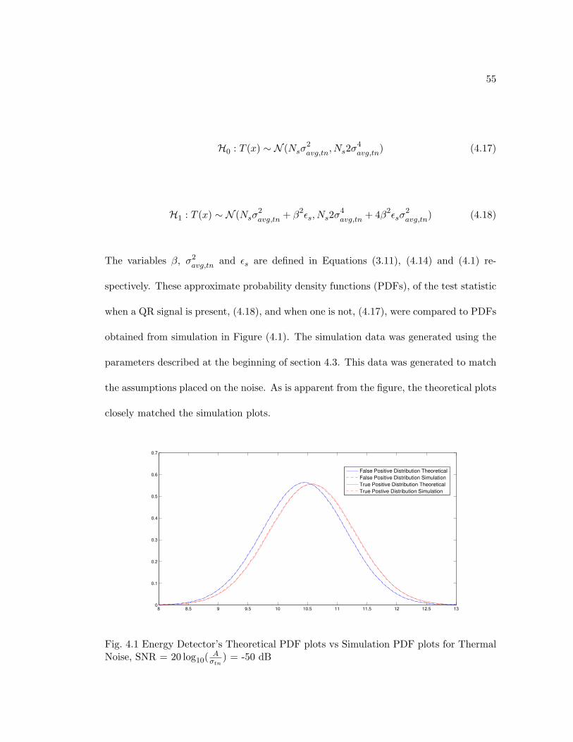
55
H0 : T (x) ∼ N (Nsσ2avg,tn
, Ns2σ4avg,tn
) (4.17)
H1 : T (x) ∼ N (Nsσ2avg,tn
+ β2εs, Ns2σ4avg,tn
+ 4β2εsσ2avg,tn
) (4.18)
The variables β, σ2avg,tn
and εs are defined in Equations (3.11), (4.14) and (4.1) re-
spectively. These approximate probability density functions (PDFs), of the test statistic
when a QR signal is present, (4.18), and when one is not, (4.17), were compared to PDFs
obtained from simulation in Figure (4.1). The simulation data was generated using the
parameters described at the beginning of section 4.3. This data was generated to match
the assumptions placed on the noise. As is apparent from the figure, the theoretical plots
closely matched the simulation plots.
8 8.5 9 9.5 10 10.5 11 11.5 12 12.5 130
0.1
0.2
0.3
0.4
0.5
0.6
0.7
False Positive Distribution Theoretical
False Positive Distribution Simulation
True Positive Distribution Theoretical
True Postive Distribution Simulation
Fig. 4.1 Energy Detector’s Theoretical PDF plots vs Simulation PDF plots for ThermalNoise, SNR = 20 log10( A
σtn) = -50 dB
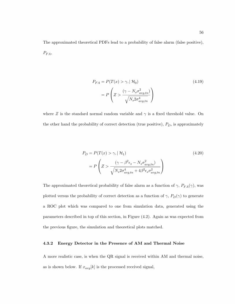
56
The approximated theoretical PDFs lead to a probability of false alarm (false positive),
PFA,
PFA = P (T (x) > γ, | H0) (4.19)
= P
Z >(γ −Nsσ
2avg,tn
)√Ns2σ4
avg,tn
where Z is the standard normal random variable and γ is a fixed threshold value. On
the other hand the probability of correct detection (true positive), PD, is approximately
PD = P (T (x) > γ, | H1) (4.20)
= P
Z >(γ − β2εs −Nsσ
2avg,tn
)√Ns2σ4
avg,tn+ 4β2εsσ
2avg,tn
The approximated theoretical probability of false alarm as a function of γ, PFA(γ), was
plotted versus the probability of correct detection as a function of γ, PD(γ) to generate
a ROC plot which was compared to one from simulation data, generated using the
parameters described in top of this section, in Figure (4.2). Again as was expected from
the previous figure, the simulation and theoretical plots matched.
4.3.2 Energy Detector in the Presence of AM and Thermal Noise
A more realistic case, is when the QR signal is received within AM and thermal noise,
as is shown below. If xavg[k] is the processed received signal,
57
0 0.1 0.2 0.3 0.4 0.5 0.6 0.7 0.8 0.9 10
0.1
0.2
0.3
0.4
0.5
0.6
0.7
0.8
0.9
1
PFA
, Probability of False Alarm
PD
, P
robabili
ty o
f C
orr
ect D
ete
ction
ROC in the presence of Thermal Noise, SNR −50 dB = 20log10
(A/σtn
)
Theoretical ROC, Energy Detector
Simulation ROC, Energy Detector
Guess
Fig. 4.2 Energy Detector’s, Theoretical ROC plot vs Simulation ROC plot for ThermalNoise, SNR = 20 log10( A
σtn) = -50 dB
H0 : xavg[k] = ηavg[k] + navg[k] (4.21)
H1 : xavg[k] = savg[k] + ηavg[k] + navg[k] (4.22)
where savg[k], ηavg[k] and navg[k] are the averaged QR signal, AM signal and the white
gaussian thermal noise signal described in Equations (3.18), (3.19) and (3.20). The
gaussian thermal noise signal has a variance of σ2avg,tn
, defined in Equation (4.14). By
definition, the noise Assumptions 3 and 4, and the fact that the AM and thermal noise
sources are independent, the test statistic is the sum of Ns independent random variables.
Since Ns is large, the test statistic can be approximated as a gaussian random variable
58
by the central limit theorem. This random variable, in the presence of AM and thermal
noise, has the following approximate distributions
H0 : T (x) ∼ N (µE,FA, σ2E,FA
) (4.23)
H1 : T (x) ∼ N (µE,D, σ2E,D
) (4.24)
for the cases shown in Equations (4.21) and (4.22) respectively. The values of µE,FA,
σ2E,FA
, µE,D and σ2E,D
are defined as follows,
µE,FA = Ns
(σ2avg,tn
+A2η
2NeNm
σ2m
2
)
σ2E,FA
= Ns
(A4η
(2NeNm)2
3σ4m
4+ 2σ4
avg,tn+ 4
(σ2avg,tn
) A2η
2NeNm
σ2m
2
)
µE,D = µE,FA + β2εs
σ2E,D
= σ2E,FA
+ 4β2εs
(A2η
2NeNm
σ2m
2+ σ2
avg,tn
)
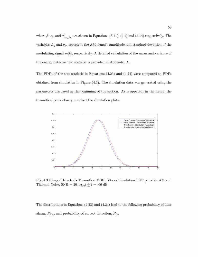
59
where β, εs, and σ2avg,tn
are shown in Equations (3.11), (4.1) and (4.14) respectively. The
variables Aη and σm represent the AM signal’s amplitude and standard deviation of the
modulating signal m[k], respectively. A detailed calculation of the mean and variance of
the energy detector test statistic is provided in Appendix A.
The PDFs of the test statistic in Equations (4.23) and (4.24) were compared to PDFs
obtained from simulation in Figure (4.3). The simulation data was generated using the
parameters discussed in the beginning of the section. As is apparent in the figure, the
theoretical plots closely matched the simulation plots.
9 10 11 12 13 14 15 16 17 18 19 200
0.05
0.1
0.15
0.2
0.25
0.3
0.35
0.4
False Positive Distribution Theoretical
False Positive Distribution Simulation
True Positive Distribution Theoretical
True Postive Distribution Simulation
Fig. 4.3 Energy Detector’s Theoretical PDF plots vs Simulation PDF plots for AM andThermal Noise, SNR = 20 log10( A
Aη) = -66 dB
The distributions in Equations (4.23) and (4.24) lead to the following probability of false
alarm, PFA, and probability of correct detection, PD,
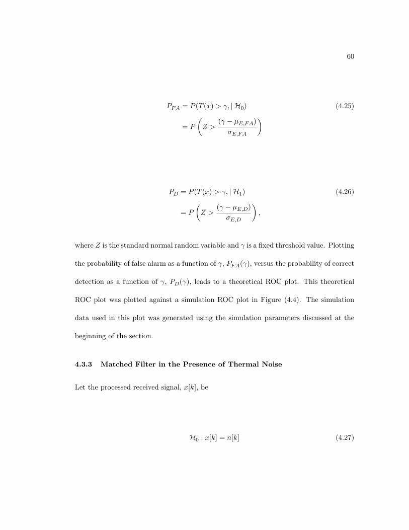
60
PFA = P (T (x) > γ, | H0) (4.25)
= P
(Z >
(γ − µE,FA)σE,FA
)
PD = P (T (x) > γ, | H1) (4.26)
= P
(Z >
(γ − µE,D)σE,D
),
where Z is the standard normal random variable and γ is a fixed threshold value. Plotting
the probability of false alarm as a function of γ, PFA(γ), versus the probability of correct
detection as a function of γ, PD(γ), leads to a theoretical ROC plot. This theoretical
ROC plot was plotted against a simulation ROC plot in Figure (4.4). The simulation
data used in this plot was generated using the simulation parameters discussed at the
beginning of the section.
4.3.3 Matched Filter in the Presence of Thermal Noise
Let the processed received signal, x[k], be
H0 : x[k] = n[k] (4.27)
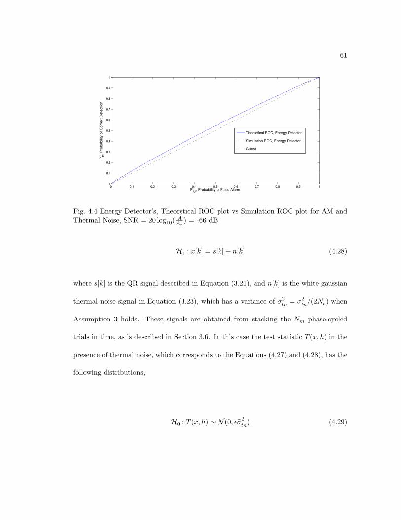
61
0 0.1 0.2 0.3 0.4 0.5 0.6 0.7 0.8 0.9 10
0.1
0.2
0.3
0.4
0.5
0.6
0.7
0.8
0.9
1
PFA
, Probability of False Alarm
PD
, P
robabili
ty o
f C
orr
ect D
ete
ction
Theoretical ROC, Energy Detector
Simulation ROC, Energy Detector
Guess
Fig. 4.4 Energy Detector’s, Theoretical ROC plot vs Simulation ROC plot for AM andThermal Noise, SNR = 20 log10( A
Aη) = -66 dB
H1 : x[k] = s[k] + n[k] (4.28)
where s[k] is the QR signal described in Equation (3.21), and n[k] is the white gaussian
thermal noise signal in Equation (3.23), which has a variance of σ2tn
= σ2tn/(2Ne) when
Assumption 3 holds. These signals are obtained from stacking the Nm phase-cycled
trials in time, as is described in Section 3.6. In this case the test statistic T (x, h) in the
presence of thermal noise, which corresponds to the Equations (4.27) and (4.28), has the
following distributions,
H0 : T (x, h) ∼ N (0, εσ2tn
) (4.29)

62
H1 : T (x, h) ∼ N (βε, εσ2tn
). (4.30)
The values of β (the decaying factor of the QR signal), σ2tn
(the variance of the phase
cycled thermal noise), and ε (the energy of the Nm QR signals without a decaying factor)
are defined in Equations (3.11), (4.13) and (4.2) respectively. The theoretical PDFs in
Equations (4.29) and (4.30) are plotted versus simulation PDFs in Figure (4.5). The
simulation PDFs were generated from data that matches the assumptions placed on the
noise with the parameters discussed at the beginning of the section. The theoretical
PDFs plotted closely match the simulation PDFs plotted and the slight discrepancy
is due to using a finite number of experiments to estimate the simulation PDFs. The
theoretical PDFs in Equations (4.29) and (4.30) lead to a probability of false alarm, PFA,
and a probability of correct detection, PD, defined as
PFA = P (T (x, s) > γ, | H0) = P
(Z > γ/
√εσ2tn
), (4.31)
PD = P (T (x, s) > γ, | H1) = P
(Z > (γ − βε)/
√εσ2tn
), (4.32)
where Z is the standard normal random variable and γ is a fixed threshold value. Plotting
the probability of false alarm as a function of γ, PFA(γ), versus the probability of the
correct detection as a function of γ, PD(γ), results in a theoretical ROC plot. This
plot and an ROC plot generated through simulation, using the simulation parameters
mentioned at the beginning of the section, are plotted in Figure (4.6) and the match is
63
apparent. The theoretical and simulation ROC plots for the energy detecter are shown
on the same figure for comparison purposes. The improvement in performance when
using the matched filter becomes apparent.
−600 −400 −200 0 200 400 600 800 10000
0.5
1
1.5
2
2.5
3x 10
−3
PFA
Theoretical PDF, −50 dB
PD
Theoretical PDF, −50 dB
PFA
Simulation PDF, −50 dB, 500 Experiments
PD
Simulation PDF, −50 dB, 500 Experiments
Fig. 4.5 Matched Filter’s Theoretical PDF plots vs Simulation PDF plots for ThermalNoise, SNR = 20 log10( A
σtn) =-50 dB
4.3.4 Matched Filter in the Presence of AM and Thermal Noise
Now considering the matched filter case, where the processed received signal, x[k], is
H0 : x[k] = η[k] + n[k], (4.33)
H1 : x[k] = s[k] + η[k] + n[k], (4.34)
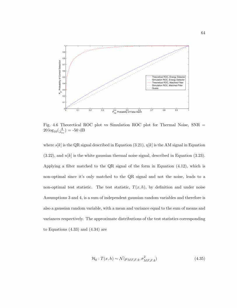
64
0 0.1 0.2 0.3 0.4 0.5 0.6 0.7 0.8 0.9 10
0.1
0.2
0.3
0.4
0.5
0.6
0.7
0.8
0.9
1
PFA
, Probability of False Alarm
PD
, P
robabili
ty o
f C
orr
ect D
ete
ction
Theoretical ROC, Energy Detector
Simulation ROC, Energy Detector
Theoretical ROC, Matched Filter
Simulation ROC, Matched Filter
Guess
Fig. 4.6 Theoretical ROC plot vs Simulation ROC plot for Thermal Noise, SNR =20 log10( A
σtn) = -50 dB
where s[k] is the QR signal described in Equation (3.21), η[k] is the AM signal in Equation
(3.22), and n[k] is the white gaussian thermal noise signal, described in Equation (3.23).
Applying a filter matched to the QR signal of the form in Equation (4.12), which is
non-optimal since it’s only matched to the QR signal and not the noise, leads to a
non-optimal test statistic. The test statistic, T (x, h), by definition and under noise
Assumptions 3 and 4, is a sum of independent gaussian random variables and therefore is
also a gaussian random variable, with a mean and variance equal to the sum of means and
variances respectively. The approximate distributions of the test statistics corresponding
to Equations (4.33) and (4.34) are
H0 : T (x, h) ∼ N (µMF,FA, σ2MF,FA
) (4.35)
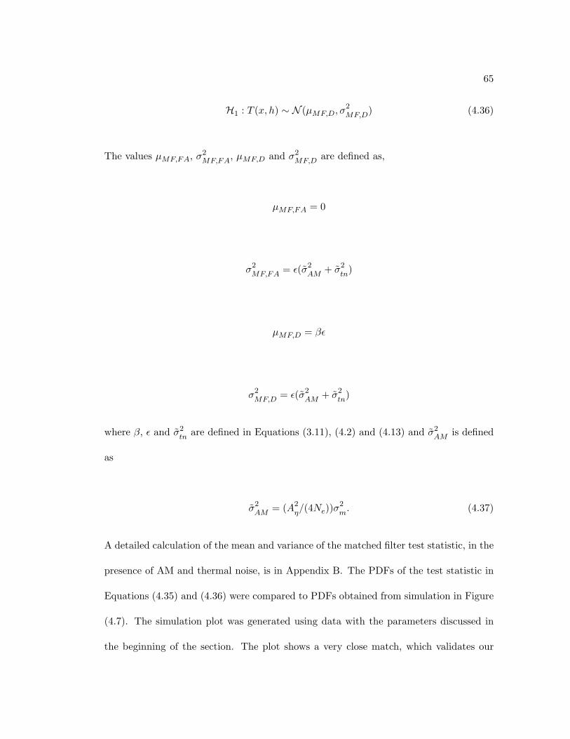
65
H1 : T (x, h) ∼ N (µMF,D, σ2MF,D
) (4.36)
The values µMF,FA, σ2MF,FA
, µMF,D and σ2MF,D
are defined as,
µMF,FA = 0
σ2MF,FA
= ε(σ2AM
+ σ2tn
)
µMF,D = βε
σ2MF,D
= ε(σ2AM
+ σ2tn
)
where β, ε and σ2tn
are defined in Equations (3.11), (4.2) and (4.13) and σ2AM
is defined
as
σ2AM
= (A2η/(4Ne))σ
2m. (4.37)
A detailed calculation of the mean and variance of the matched filter test statistic, in the
presence of AM and thermal noise, is in Appendix B. The PDFs of the test statistic in
Equations (4.35) and (4.36) were compared to PDFs obtained from simulation in Figure
(4.7). The simulation plot was generated using data with the parameters discussed in
the beginning of the section. The plot shows a very close match, which validates our
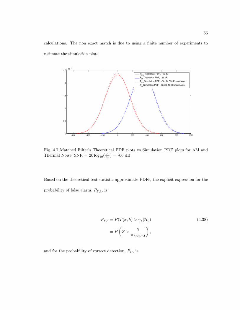
66
calculations. The non exact match is due to using a finite number of experiments to
estimate the simulation plots.
−600 −400 −200 0 200 400 600 800 10000
0.5
1
1.5
2
2.5x 10
−3
PFA
Theoretical PDF, −66 dB
PD
Theoretical PDF, −66 dB
PFA
Simulation PDF, −66 dB, 500 Experiments
PD
Simulation PDF, −66 dB, 500 Experiments
Fig. 4.7 Matched Filter’s Theoretical PDF plots vs Simulation PDF plots for AM andThermal Noise, SNR = 20 log10( A
Aη) = -66 dB
Based on the theoretical test statistic approximate PDFs, the explicit expression for the
probability of false alarm, PFA, is
PFA = P (T (x, h) > γ, |H0) (4.38)
= P
(Z >
γ
σMF,FA
),
and for the probability of correct detection, PD, is
67
PD = P (T (x, h) > γ, |H1) (4.39)
= P
(Z >
(γ − µMF,D)σMF,D
),
where Z is the standard normal random variable and γ is a fixed threshold value. Plotting
the theoretical probability of false alarm as a function of γ, PFA(γ), versus the probability
of correct detection as a function of γ, PD(γ), generates a theoretical ROC plot. This plot
is compared to an ROC plot obtained from simulation in Figure (4.8) and the match is
apparent. As mentioned earlier, the simulation data was generated using the simulation
parameters discussed in the beginning of the section, and with the assumptions placed
on the noise when calculating the theoretical expressions. The same figure displays the
performance of the energy detector, and the improvement in performance when utilizing
information about the signal is apparent.
4.3.5 Thermal Noise Comparison
When comparing the performance of the matched filter to the energy detector in Figure
(4.6), the improvement is significant. In the case of gaussian noise, not utilizing the shape
of the QR signal and squaring the received signal, as in the energy detector, makes the
first moment of the test statistic a function of the second moment of the noise, which is
nonzero. This brings the PDF of the test statistic in the case of no QR signal closer to
the PDF of the test statistic when a QR signal is present. On the other hand the first
moment of the test statistic of the matched filter is zero when a QR signal is not present,
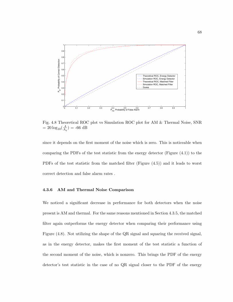
68
0 0.1 0.2 0.3 0.4 0.5 0.6 0.7 0.8 0.9 10
0.1
0.2
0.3
0.4
0.5
0.6
0.7
0.8
0.9
1
PFA
, Probability of False Alarm
PD
, P
robabili
ty o
f C
orr
ect D
ete
ction
Theoretical ROC, Energy Detector
Simulation ROC, Energy Detector
Theoretical ROC, Matched Filter
Simulation ROC, Matched Filter
Guess
Fig. 4.8 Theoretical ROC plot vs Simulation ROC plot for AM & Thermal Noise, SNR= 20 log10( A
Aη) = -66 dB
since it depends on the first moment of the noise which is zero. This is noticeable when
comparing the PDFs of the test statistic from the energy detector (Figure (4.1)) to the
PDFs of the test statistic from the matched filter (Figure (4.5)) and it leads to worst
correct detection and false alarm rates .
4.3.6 AM and Thermal Noise Comparison
We noticed a significant decrease in performance for both detectors when the noise
present is AM and thermal. For the same reasons mentioned in Section 4.3.5, the matched
filter again outperforms the energy detector when comparing their performance using
Figure (4.8). Not utilizing the shape of the QR signal and squaring the received signal,
as in the energy detector, makes the first moment of the test statistic a function of
the second moment of the noise, which is nonzero. This brings the PDF of the energy
detector’s test statistic in the case of no QR signal closer to the PDF of the energy
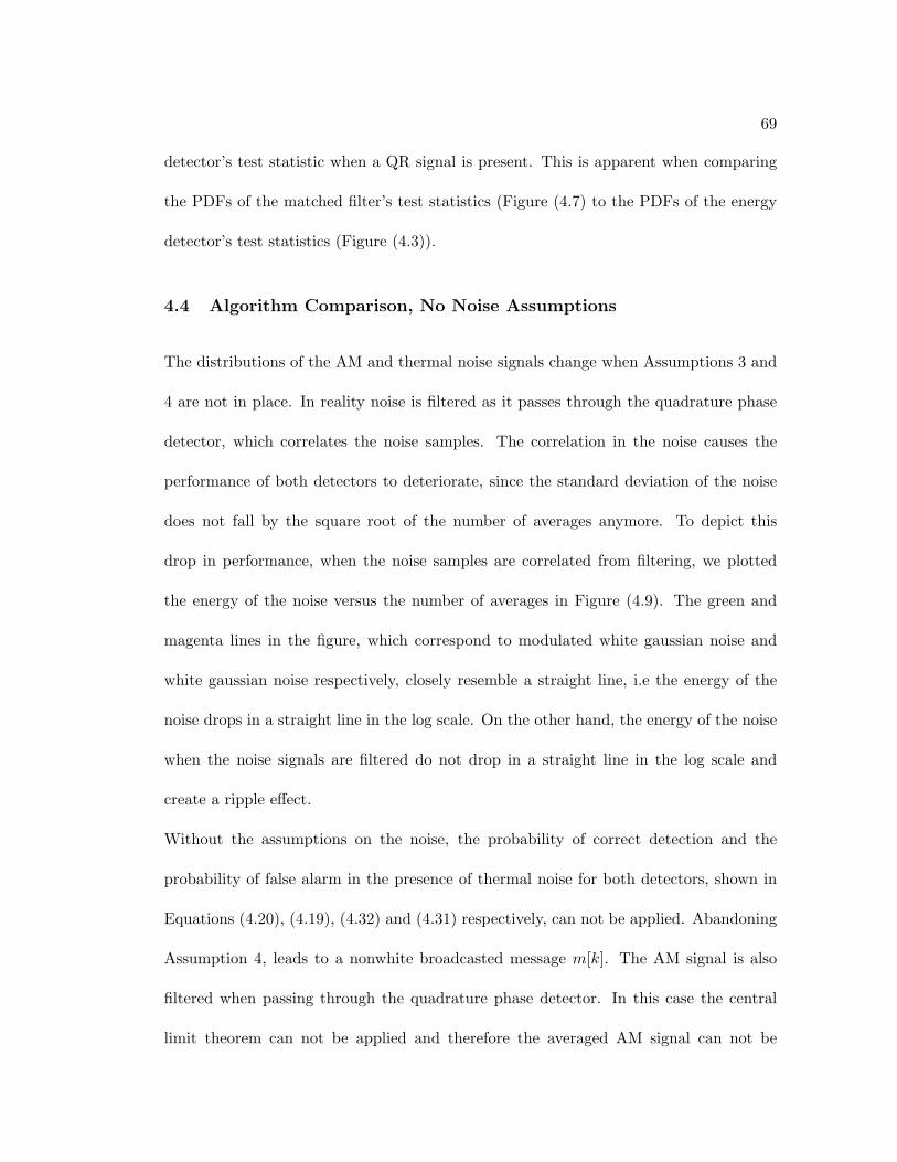
69
detector’s test statistic when a QR signal is present. This is apparent when comparing
the PDFs of the matched filter’s test statistics (Figure (4.7) to the PDFs of the energy
detector’s test statistics (Figure (4.3)).
4.4 Algorithm Comparison, No Noise Assumptions
The distributions of the AM and thermal noise signals change when Assumptions 3 and
4 are not in place. In reality noise is filtered as it passes through the quadrature phase
detector, which correlates the noise samples. The correlation in the noise causes the
performance of both detectors to deteriorate, since the standard deviation of the noise
does not fall by the square root of the number of averages anymore. To depict this
drop in performance, when the noise samples are correlated from filtering, we plotted
the energy of the noise versus the number of averages in Figure (4.9). The green and
magenta lines in the figure, which correspond to modulated white gaussian noise and
white gaussian noise respectively, closely resemble a straight line, i.e the energy of the
noise drops in a straight line in the log scale. On the other hand, the energy of the noise
when the noise signals are filtered do not drop in a straight line in the log scale and
create a ripple effect.
Without the assumptions on the noise, the probability of correct detection and the
probability of false alarm in the presence of thermal noise for both detectors, shown in
Equations (4.20), (4.19), (4.32) and (4.31) respectively, can not be applied. Abandoning
Assumption 4, leads to a nonwhite broadcasted message m[k]. The AM signal is also
filtered when passing through the quadrature phase detector. In this case the central
limit theorem can not be applied and therefore the averaged AM signal can not be
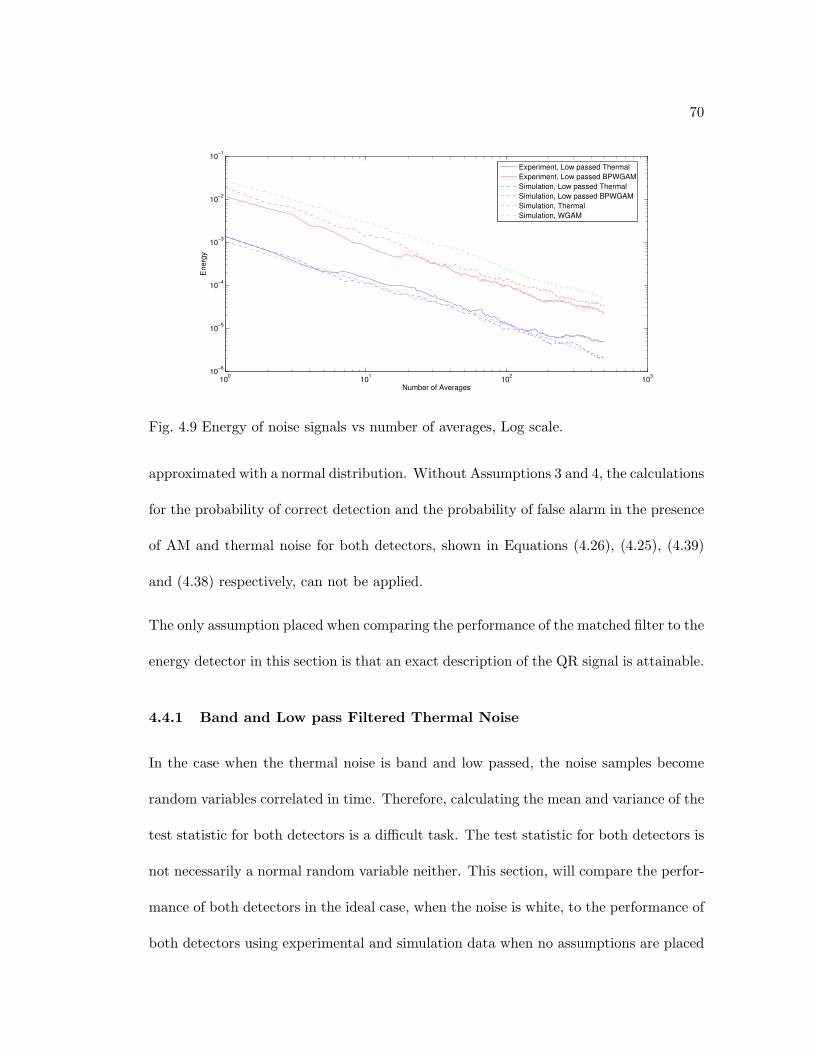
70
100
101
102
103
10−6
10−5
10−4
10−3
10−2
10−1
Number of Averages
Energ
y
Experiment, Low passed Thermal
Experiment, Low passed BPWGAM
Simulation, Low passed Thermal
Simulation, Low passed BPWGAM
Simulation, Thermal
Simulation, WGAM
Fig. 4.9 Energy of noise signals vs number of averages, Log scale.
approximated with a normal distribution. Without Assumptions 3 and 4, the calculations
for the probability of correct detection and the probability of false alarm in the presence
of AM and thermal noise for both detectors, shown in Equations (4.26), (4.25), (4.39)
and (4.38) respectively, can not be applied.
The only assumption placed when comparing the performance of the matched filter to the
energy detector in this section is that an exact description of the QR signal is attainable.
4.4.1 Band and Low pass Filtered Thermal Noise
In the case when the thermal noise is band and low passed, the noise samples become
random variables correlated in time. Therefore, calculating the mean and variance of the
test statistic for both detectors is a difficult task. The test statistic for both detectors is
not necessarily a normal random variable neither. This section, will compare the perfor-
mance of both detectors in the ideal case, when the noise is white, to the performance of
both detectors using experimental and simulation data when no assumptions are placed
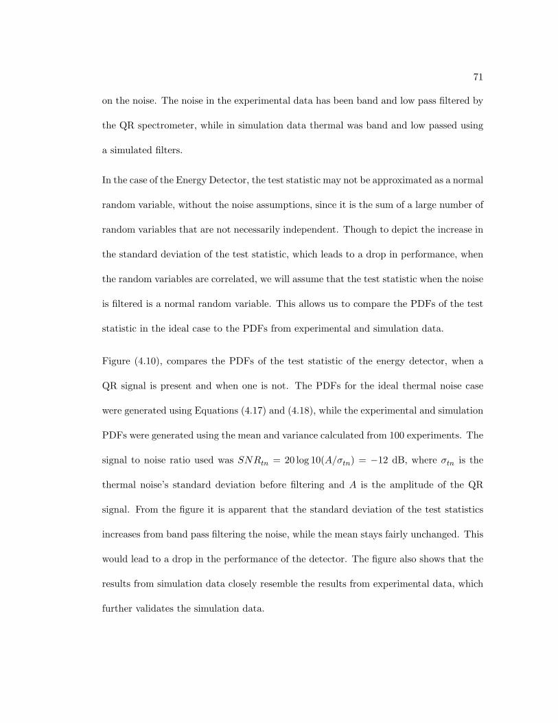
71
on the noise. The noise in the experimental data has been band and low pass filtered by
the QR spectrometer, while in simulation data thermal was band and low passed using
a simulated filters.
In the case of the Energy Detector, the test statistic may not be approximated as a normal
random variable, without the noise assumptions, since it is the sum of a large number of
random variables that are not necessarily independent. Though to depict the increase in
the standard deviation of the test statistic, which leads to a drop in performance, when
the random variables are correlated, we will assume that the test statistic when the noise
is filtered is a normal random variable. This allows us to compare the PDFs of the test
statistic in the ideal case to the PDFs from experimental and simulation data.
Figure (4.10), compares the PDFs of the test statistic of the energy detector, when a
QR signal is present and when one is not. The PDFs for the ideal thermal noise case
were generated using Equations (4.17) and (4.18), while the experimental and simulation
PDFs were generated using the mean and variance calculated from 100 experiments. The
signal to noise ratio used was SNRtn = 20 log 10(A/σtn) = −12 dB, where σtn is the
thermal noise’s standard deviation before filtering and A is the amplitude of the QR
signal. From the figure it is apparent that the standard deviation of the test statistics
increases from band pass filtering the noise, while the mean stays fairly unchanged. This
would lead to a drop in the performance of the detector. The figure also shows that the
results from simulation data closely resemble the results from experimental data, which
further validates the simulation data.
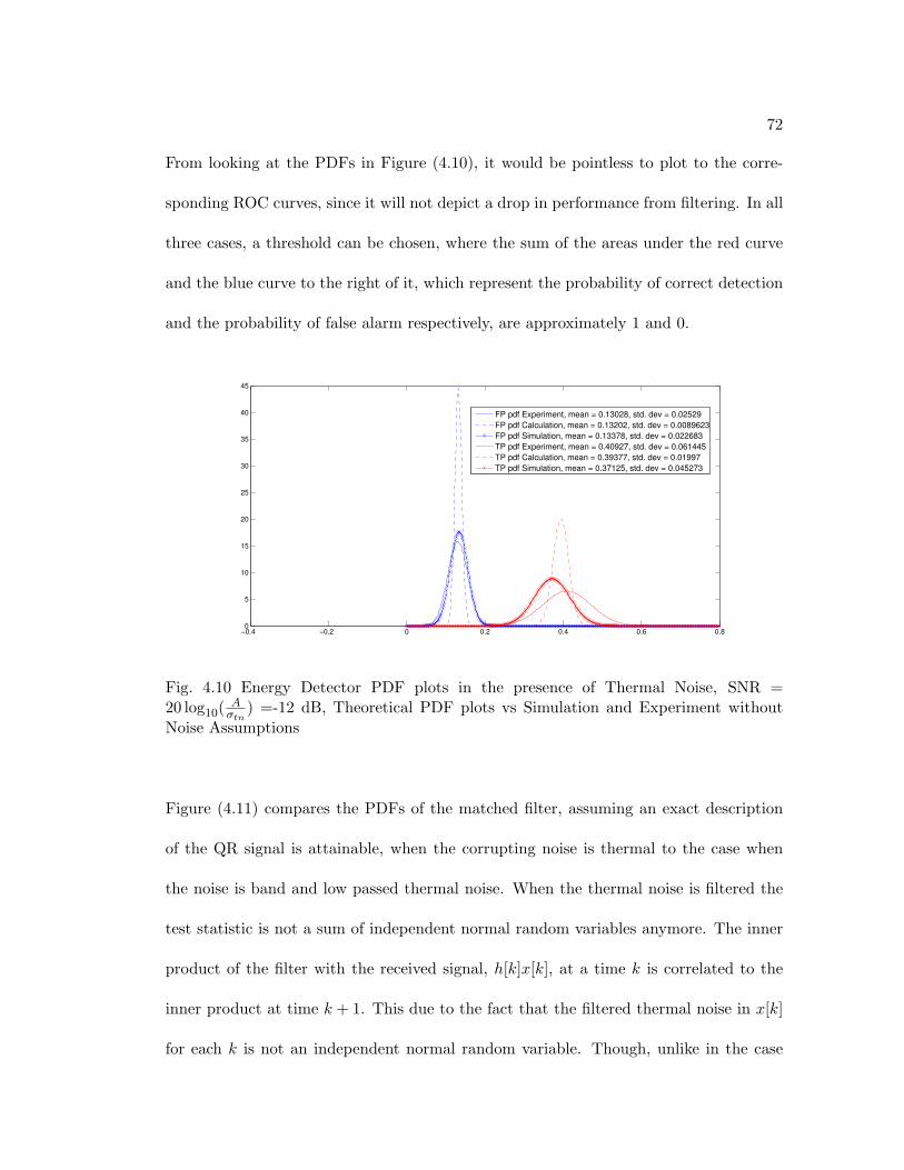
72
From looking at the PDFs in Figure (4.10), it would be pointless to plot to the corre-
sponding ROC curves, since it will not depict a drop in performance from filtering. In all
three cases, a threshold can be chosen, where the sum of the areas under the red curve
and the blue curve to the right of it, which represent the probability of correct detection
and the probability of false alarm respectively, are approximately 1 and 0.
−0.4 −0.2 0 0.2 0.4 0.6 0.80
5
10
15
20
25
30
35
40
45
FP pdf Experiment, mean = 0.13028, std. dev = 0.02529
FP pdf Calculation, mean = 0.13202, std. dev = 0.0089623
FP pdf Simulation, mean = 0.13378, std. dev = 0.022683
TP pdf Experiment, mean = 0.40927, std. dev = 0.061445
TP pdf Calculation, mean = 0.39377, std. dev = 0.01997
TP pdf Simulation, mean = 0.37125, std. dev = 0.045273
Fig. 4.10 Energy Detector PDF plots in the presence of Thermal Noise, SNR =20 log10( A
σtn) =-12 dB, Theoretical PDF plots vs Simulation and Experiment without
Noise Assumptions
Figure (4.11) compares the PDFs of the matched filter, assuming an exact description
of the QR signal is attainable, when the corrupting noise is thermal to the case when
the noise is band and low passed thermal noise. When the thermal noise is filtered the
test statistic is not a sum of independent normal random variables anymore. The inner
product of the filter with the received signal, h[k]x[k], at a time k is correlated to the
inner product at time k + 1. This due to the fact that the filtered thermal noise in x[k]
for each k is not an independent normal random variable. Though, unlike in the case
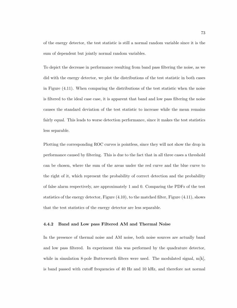
73
of the energy detector, the test statistic is still a normal random variable since it is the
sum of dependent but jointly normal random variables.
To depict the decrease in performance resulting from band pass filtering the noise, as we
did with the energy detector, we plot the distributions of the test statistic in both cases
in Figure (4.11). When comparing the distributions of the test statistic when the noise
is filtered to the ideal case case, it is apparent that band and low pass filtering the noise
causes the standard deviation of the test statistic to increase while the mean remains
fairly equal. This leads to worse detection performance, since it makes the test statistics
less separable.
Plotting the corresponding ROC curves is pointless, since they will not show the drop in
performance caused by filtering. This is due to the fact that in all three cases a threshold
can be chosen, where the sum of the areas under the red curve and the blue curve to
the right of it, which represent the probability of correct detection and the probability
of false alarm respectively, are approximately 1 and 0. Comparing the PDFs of the test
statistics of the energy detector, Figure (4.10), to the matched filter, Figure (4.11), shows
that the test statistics of the energy detector are less separable.
4.4.2 Band and Low pass Filtered AM and Thermal Noise
In the presence of thermal noise and AM noise, both noise sources are actually band
and low pass filtered. In experiment this was performed by the quadrature detector,
while in simulation 8-pole Butterworth filters were used. The modulated signal, m[k],
is band passed with cutoff frequencies of 40 Hz and 10 kHz, and therefore not normal
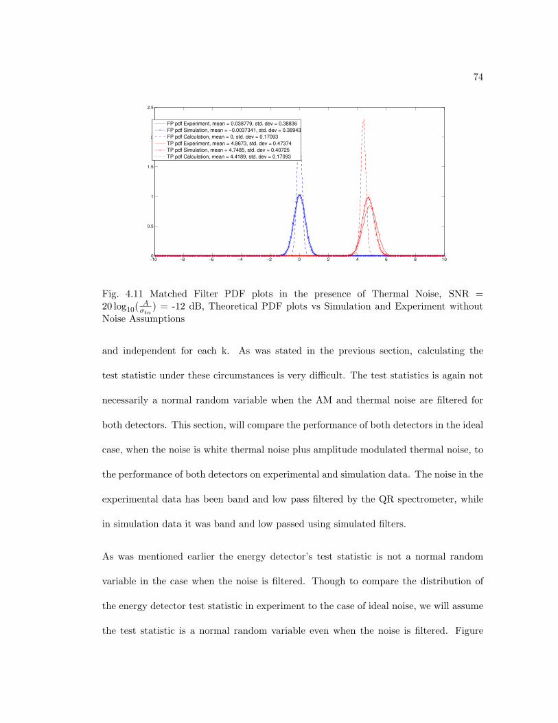
74
−10 −8 −6 −4 −2 0 2 4 6 8 100
0.5
1
1.5
2
2.5
FP pdf Experiment, mean = 0.038779, std. dev = 0.38836
FP pdf Simulation, mean = −0.0037341, std. dev = 0.38943
FP pdf Calculation, mean = 0, std. dev = 0.17093
TP pdf Experiment, mean = 4.8673, std. dev = 0.47374
TP pdf Simulation, mean = 4.7485, std. dev = 0.40725
TP pdf Calculation, mean = 4.4189, std. dev = 0.17093
Fig. 4.11 Matched Filter PDF plots in the presence of Thermal Noise, SNR =20 log10( A
σtn) = -12 dB, Theoretical PDF plots vs Simulation and Experiment without
Noise Assumptions
and independent for each k. As was stated in the previous section, calculating the
test statistic under these circumstances is very difficult. The test statistics is again not
necessarily a normal random variable when the AM and thermal noise are filtered for
both detectors. This section, will compare the performance of both detectors in the ideal
case, when the noise is white thermal noise plus amplitude modulated thermal noise, to
the performance of both detectors on experimental and simulation data. The noise in the
experimental data has been band and low pass filtered by the QR spectrometer, while
in simulation data it was band and low passed using simulated filters.
As was mentioned earlier the energy detector’s test statistic is not a normal random
variable in the case when the noise is filtered. Though to compare the distribution of
the energy detector test statistic in experiment to the case of ideal noise, we will assume
the test statistic is a normal random variable even when the noise is filtered. Figure
75
(4.12) compares the distributions of the test statistic from calculation, Equations (4.23)
and (4.24), to the test statistics from experimental and simulation data when no noise
is filtered. The mean and variance of the test statistics for experimental and simulation
data, where calculated based on 50 experiments. As is in the previous section these plots
depict the increase in the standard deviation of the test statistic in the case of filtered
noise, which is due to the correlation in the noise samples after filtering. The plot also
shows that the test statistic from simulation data is very close to the test statistic from
experimental data. This increase in standard deviation decreases the performance level
of the energy detector. The corresponding ROC plots are shown in Figure (4.13). As
expected, the energy detector in the ideal uncorrelated noise case, outperforms the energy
detector when applied to experimental and simulation data with filtered noise.
−1 0 1 2 3 4 50
1
2
3
4
5
6
7
8
FP pdf Experiment, mean = 0.50791, std. dev = 0.092221
FP pdf Calculation, mean = 0.67632, std. dev = 0.054462
FP pdf Simulation, mean = 0.51913, std. dev = 0.090475TP pdf Experiment, mean = 0.72802, std. dev = 0.13476
TP pdf Calculation, mean = 0.87959, std. dev = 0.065063
TP pdf Simulation, mean = 0.77613, std. dev = 0.11602
Fig. 4.12 Energy Detector PDF plots in the presence of band-passed white gaussian AMand Thermal Noise, SNR = 20 log10( A
Aη) = -30 dB, Theoretical PDF plots vs Simulation
and Experiment without Noise Assumptions. Nm = 10, Number of experiments = 50.
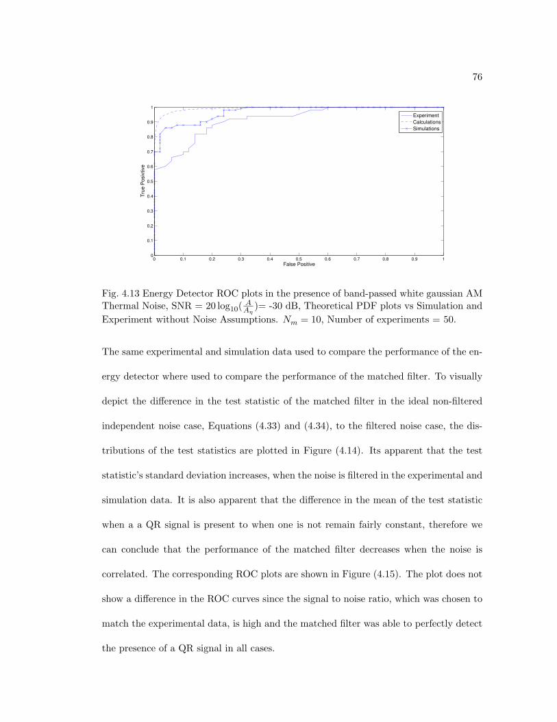
76
0 0.1 0.2 0.3 0.4 0.5 0.6 0.7 0.8 0.9 10
0.1
0.2
0.3
0.4
0.5
0.6
0.7
0.8
0.9
1
False Positive
Tru
e P
osiv
tive
Experiment
Calculations
Simulations
Fig. 4.13 Energy Detector ROC plots in the presence of band-passed white gaussian AMThermal Noise, SNR = 20 log10( A
Aη)= -30 dB, Theoretical PDF plots vs Simulation and
Experiment without Noise Assumptions. Nm = 10, Number of experiments = 50.
The same experimental and simulation data used to compare the performance of the en-
ergy detector where used to compare the performance of the matched filter. To visually
depict the difference in the test statistic of the matched filter in the ideal non-filtered
independent noise case, Equations (4.33) and (4.34), to the filtered noise case, the dis-
tributions of the test statistics are plotted in Figure (4.14). Its apparent that the test
statistic’s standard deviation increases, when the noise is filtered in the experimental and
simulation data. It is also apparent that the difference in the mean of the test statistic
when a a QR signal is present to when one is not remain fairly constant, therefore we
can conclude that the performance of the matched filter decreases when the noise is
correlated. The corresponding ROC plots are shown in Figure (4.15). The plot does not
show a difference in the ROC curves since the signal to noise ratio, which was chosen to
match the experimental data, is high and the matched filter was able to perfectly detect
the presence of a QR signal in all cases.
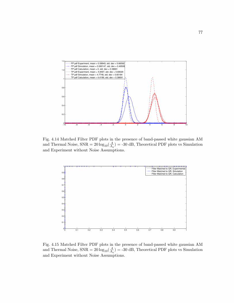
77
−10 −8 −6 −4 −2 0 2 4 6 8 100
0.2
0.4
0.6
0.8
1
1.2
1.4
FP pdf Experiment, mean = 0.58943, std. dev = 0.66592
FP pdf Simulation, mean = 0.060147, std. dev = 0.49506
FP pdf Calculation, mean = 0, std. dev = 0.38691
TP pdf Experiment, mean = 4.8467, std. dev = 0.69029
TP pdf Simulation, mean = 4.7748, std. dev = 0.60184
TP pdf Calculation, mean = 4.4189, std. dev = 0.38691
Fig. 4.14 Matched Filter PDF plots in the presence of band-passed white gaussian AMand Thermal Noise, SNR = 20 log10( A
Aη) = -30 dB, Theoretical PDF plots vs Simulation
and Experiment without Noise Assumptions.
0 0.1 0.2 0.3 0.4 0.5 0.6 0.7 0.8 0.9 10
0.1
0.2
0.3
0.4
0.5
0.6
0.7
0.8
0.9
1
Filter Matched to QR, Experimental
Filter Matched to QR, Simulation
Filter Matched to QR, Calculation
Fig. 4.15 Matched Filter PDF plots in the presence of band-passed white gaussian AMand Thermal Noise, SNR = 20 log10( A
Aη) = -30 dB, Theoretical PDF plots vs Simulation
and Experiment without Noise Assumptions.
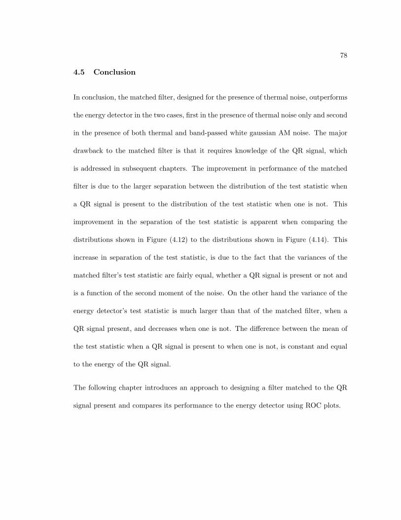
78
4.5 Conclusion
In conclusion, the matched filter, designed for the presence of thermal noise, outperforms
the energy detector in the two cases, first in the presence of thermal noise only and second
in the presence of both thermal and band-passed white gaussian AM noise. The major
drawback to the matched filter is that it requires knowledge of the QR signal, which
is addressed in subsequent chapters. The improvement in performance of the matched
filter is due to the larger separation between the distribution of the test statistic when
a QR signal is present to the distribution of the test statistic when one is not. This
improvement in the separation of the test statistic is apparent when comparing the
distributions shown in Figure (4.12) to the distributions shown in Figure (4.14). This
increase in separation of the test statistic, is due to the fact that the variances of the
matched filter’s test statistic are fairly equal, whether a QR signal is present or not and
is a function of the second moment of the noise. On the other hand the variance of the
energy detector’s test statistic is much larger than that of the matched filter, when a
QR signal present, and decreases when one is not. The difference between the mean of
the test statistic when a QR signal is present to when one is not, is constant and equal
to the energy of the QR signal.
The following chapter introduces an approach to designing a filter matched to the QR
signal present and compares its performance to the energy detector using ROC plots.
79
Chapter 5
Batch Matched Filter
As a first attempt to solving the QR detection problem, we propose a gridding approach
to determine the unknown QR parameters and design a filter matched to each value on
the grid, creating a batch of matched filters. Using the output of the batch of filters a
decision whether a QR signal is present is made.
The received corrupted version of the QR signal after Nm experiments is the sum of
the phase cycled QR, AM and thermal noise signals shown in Equations (3.21), (3.22)
and (3.23) respectively. Since the observed QR signal’s base band frequency ωbb =
ω∗ − ωs + ω0, (note that ωs was denoted as ω∗ in Section 2.4), base-band phase φbb,
and the decaying response parameter T2∗ are unknowns, we are unable to design a
periodic filter matched to the QR signal. However, we can utilize the knowledge that the
observed base band frequency ωbb, base band phase φbb and decaying parameter T2∗ fall
within known upper and lower bounds, as is shown in Equations (5.1), (5.2) and (5.3)
respectively, to design a batch of matched filters to use for QR detection.
ωlb ≤ ωbb ≤ ωub (5.1)
−π ≤ φbb ≤ π (5.2)
80
T ∗2 lb≤ T ∗
2≤ T ∗
2 ub(5.3)
Designing a matched filter for each possible frequency, phase and decaying parameter
within the bounded ranges above is not feasible. We therefore chose to discretize the
range of values, creating a grid of possible values, and design a filter matched to each
value on the grid. Out of this batch of filters, the one that results in the maximum
output is the chosen filter and its output is compared to a threshold to determine the
presence of a QR signal. Since this approach does not design a filter for each possible QR
signal that might be present, the problem where any one of the QR signal’s parameters
(frequency, phase and decaying parameter), does not match any of the values on the grid
should be addressed.
The following section discusses this problem and shows that small uncertainties in the
QR signal parameters have a small effect on the inner product of the QR signal with the
filter, which is the value that enables one to detect the presence of the QR signal. This
section is followed by a more detailed description of the “brute force” batch matched
filter algorithm, which is then followed by a section that compares the performance of
the “brute force” approach to the batch matched filter to the generic energy detector
algorithm. The improvement in performance gained from finer gridding of the parameters
is then discussed in a following section. An adaptive gridding approach to the batch
matched filter is introduced in Section 5.5. The idea behind the adaptive grid approach,
is to perform a coarse global grid and once a grid point is selected, perform a finer local
search around that point. The performance of the batch filter using this approach is then
81
compared to the “brute force” approach to the batch matched filter. Unless specified
otherwise, when referring to the batch matched filter in the subsequent chapters, the
reference is to the “brute force” approach described in Section 5.2 and not the smart
adaptive gridding approach. The chapter ends with a section that discusses possible
thresholding methods that can be used.
5.1 Error in the QR signal Description
This section addresses the issue when the frequency, phase or decaying parameter of
the matched filter are not exactly matched to the QR signal. It shows that for small
uncertainties in the QR signal parameters the performance of the matched filter is not
significantly affected, but as the error increases the performance of the filter quickly starts
to deteriorate. The drop in performance of the matched filter, is due to the drop in the
value of Equation (4.2), the inner product of the filter and the QR signal present. As
this value decreases, the mean of the test statistic when a QR signal is present becomes
closer to the mean of the test statistic when a QR signal is not. If the QR signal within
the received signal can be described as,
s[k] =A
αse(−|−T/2+k∆|/T2
∗) cos (ωbb(−T/2 + k∆) + φbb). (5.4)
for k = 0, 1, . . . , Ns− 1, where αs normalizes the signal in the l2 norm. If we assume the
error variables in frequency, phase and decaying parameter are denoted by ∆ωbb, ∆φbb,
and ∆T2∗ respectively, then the mismatched filter can be described as
82
hu[k] =B
αBe(−|−T/2+k∆|/(T2
∗+∆T2∗) cos ((ωbb + ∆ωbb)(−T/2 + k∆) + φbb + ∆φbb), (5.5)
for k = 0, 1, . . . , Ns − 1, where αB normalizes the signal in the l2 norm. With this
error, the inner product of the QR signal present and the filter, which was represented
in Equation (4.2), for Nm = 1, changes to,
εu =Ns−1∑k=0
AB
αsαh[e(−|−T/2+k∆|/T2
∗)e(−|−T/2+k∆|/(T2∗+∆T2
∗)] . . . (5.6)
[cos ((ωbb + ∆ωbb)(−T/2 + k∆) + φbb + ∆φbb) cos(ωbb(−T/2 + k∆) + φbb)]
=Ns−1∑k=0
AB
αsαh[e(−|−T/2+k∆|/T2
∗)e(−|−T/2+k∆|/(T2∗+∆T2
∗)] . . .
[cos (∆ωbb(−T/2 + k∆) + ∆φbb)− . . .
sin(ωbb(−T/2 + k∆) + φbb) sin((ωbb + ∆ωbb)(−T/2 + k∆) + φbb + ∆φbb)]
.
Next we discuss how this value changes with respect to sole changes in the error of the
individual parameters, starting with frequency. A plot of this inner product, εu versus
the error in frequency is shown in Figure (5.1), where the received QR signal had a
frequency of 12.1 kHz and the filter’s frequency error varied from 0 to 3 kHz. The plot
shows that the energy rapidly drops as the frequency offset increases causing a drop
in performance of the matched filter. Based on this plot, the gridding in frequency in
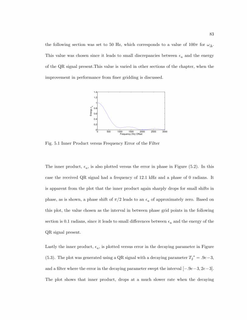
83
the following section was set to 50 Hz, which corresponds to a value of 100π for ω∆.
This value was chosen since it leads to small discrepancies between εu and the energy
of the QR signal present.This value is varied in other sections of the chapter, when the
improvement in performance from finer gridding is discussed.
0 500 1000 1500 2000 2500 30000
0.2
0.4
0.6
0.8
1
1.2
1.4E
nerg
y, ε
u
Frequency (Hz) Offset
Fig. 5.1 Inner Product versus Frequency Error of the Filter
The inner product, εu, is also plotted versus the error in phase in Figure (5.2). In this
case the received QR signal had a frequency of 12.1 kHz and a phase of 0 radians. It
is apparent from the plot that the inner product again sharply drops for small shifts in
phase, as is shown, a phase shift of π/2 leads to an εu of approximately zero. Based on
this plot, the value chosen as the interval in between phase grid points in the following
section is 0.1 radians, since it leads to small differences between εu and the energy of the
QR signal present.
Lastly the inner product, εu, is plotted versus error in the decaying parameter in Figure
(5.3). The plot was generated using a QR signal with a decaying parameter T2∗ = .9e−3,
and a filter where the error in the decaying parameter swept the interval [−.9e−3, 2e−3].
The plot shows that inner product, drops at a much slower rate when the decaying
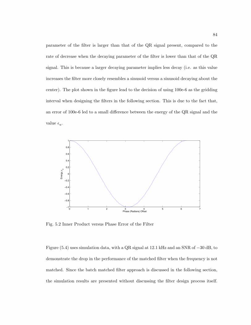
84
parameter of the filter is larger than that of the QR signal present, compared to the
rate of decrease when the decaying parameter of the filter is lower than that of the QR
signal. This is because a larger decaying parameter implies less decay (i.e. as this value
increases the filter more closely resembles a sinusoid versus a sinusoid decaying about the
center). The plot shown in the figure lead to the decision of using 100e-6 as the gridding
interval when designing the filters in the following section. This is due to the fact that,
an error of 100e-6 led to a small difference between the energy of the QR signal and the
value εu.
0 1 2 3 4 5 6 7−1
−0.8
−0.6
−0.4
−0.2
0
0.2
0.4
0.6
0.8
1
Energ
y, ε
u
Phase (Radians) Offset
Fig. 5.2 Inner Product versus Phase Error of the Filter
Figure (5.4) uses simulation data, with a QR signal at 12.1 kHz and an SNR of −30 dB, to
demonstrate the drop in the performance of the matched filter when the frequency is not
matched. Since the batch matched filter approach is discussed in the following section,
the simulation results are presented without discussing the filter design process itself.
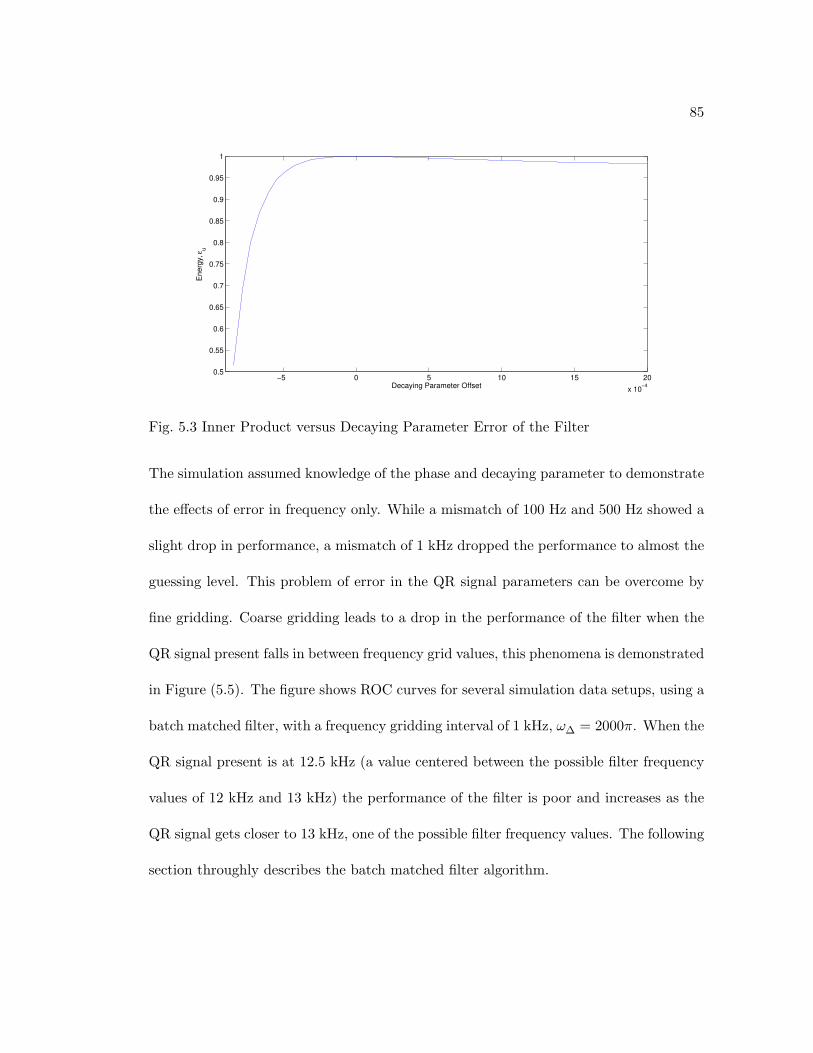
85
−5 0 5 10 15 20
x 10−4
0.5
0.55
0.6
0.65
0.7
0.75
0.8
0.85
0.9
0.95
1
Energ
y, ε
u
Decaying Parameter Offset
Fig. 5.3 Inner Product versus Decaying Parameter Error of the Filter
The simulation assumed knowledge of the phase and decaying parameter to demonstrate
the effects of error in frequency only. While a mismatch of 100 Hz and 500 Hz showed a
slight drop in performance, a mismatch of 1 kHz dropped the performance to almost the
guessing level. This problem of error in the QR signal parameters can be overcome by
fine gridding. Coarse gridding leads to a drop in the performance of the filter when the
QR signal present falls in between frequency grid values, this phenomena is demonstrated
in Figure (5.5). The figure shows ROC curves for several simulation data setups, using a
batch matched filter, with a frequency gridding interval of 1 kHz, ω∆ = 2000π. When the
QR signal present is at 12.5 kHz (a value centered between the possible filter frequency
values of 12 kHz and 13 kHz) the performance of the filter is poor and increases as the
QR signal gets closer to 13 kHz, one of the possible filter frequency values. The following
section throughly describes the batch matched filter algorithm.
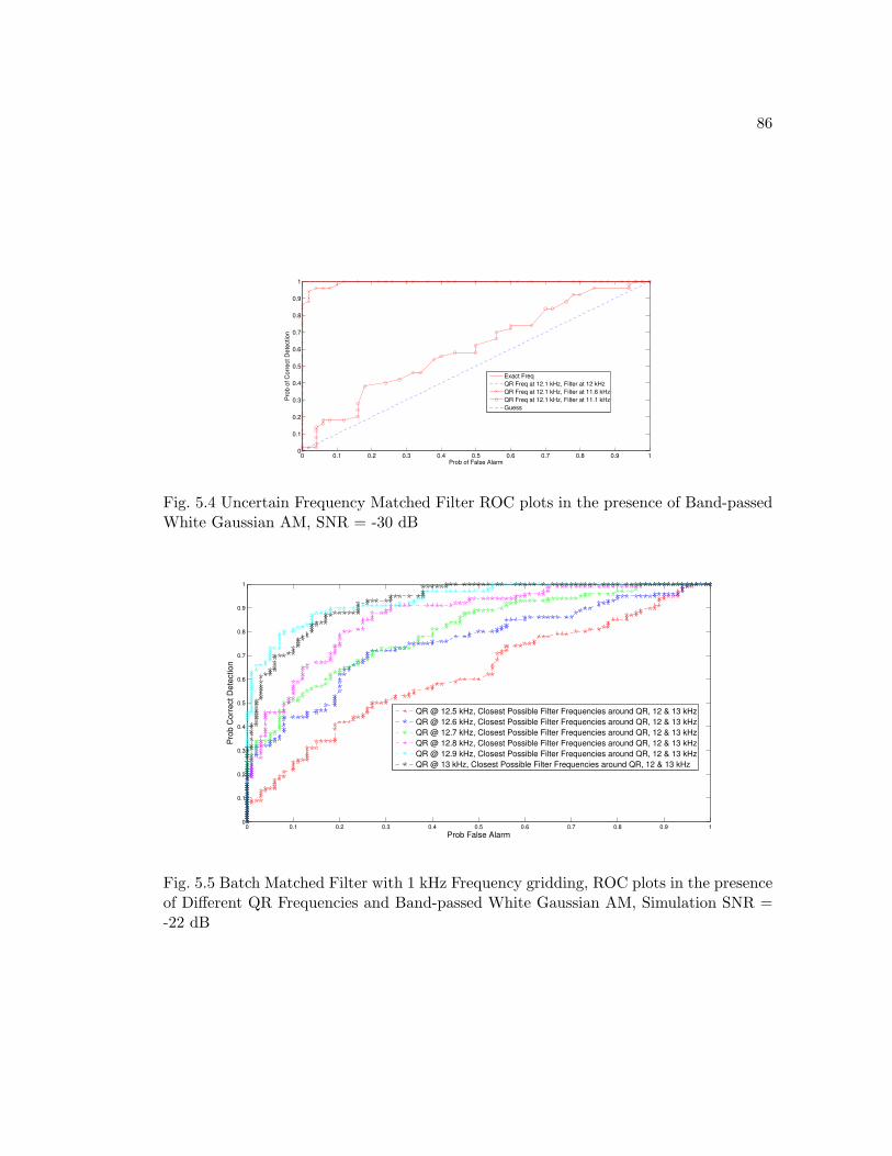
86
0 0.1 0.2 0.3 0.4 0.5 0.6 0.7 0.8 0.9 10
0.1
0.2
0.3
0.4
0.5
0.6
0.7
0.8
0.9
1
Prob of False Alarm
Pro
b o
f C
orr
ect
De
tectio
n
Exact Freq
QR Freq at 12.1 kHz, Filter at 12 kHz
QR Freq at 12.1 kHz, Filter at 11.6 kHz
QR Freq at 12.1 kHz, Filter at 11.1 kHz
Guess
Fig. 5.4 Uncertain Frequency Matched Filter ROC plots in the presence of Band-passedWhite Gaussian AM, SNR = -30 dB
0 0.1 0.2 0.3 0.4 0.5 0.6 0.7 0.8 0.9 10
0.1
0.2
0.3
0.4
0.5
0.6
0.7
0.8
0.9
1
Pro
b C
orr
ect D
ete
ction
Prob False Alarm
QR @ 12.5 kHz, Closest Possible Filter Frequencies around QR, 12 & 13 kHz
QR @ 12.6 kHz, Closest Possible Filter Frequencies around QR, 12 & 13 kHz
QR @ 12.7 kHz, Closest Possible Filter Frequencies around QR, 12 & 13 kHz
QR @ 12.8 kHz, Closest Possible Filter Frequencies around QR, 12 & 13 kHz
QR @ 12.9 kHz, Closest Possible Filter Frequencies around QR, 12 & 13 kHz
QR @ 13 kHz, Closest Possible Filter Frequencies around QR, 12 & 13 kHz
Fig. 5.5 Batch Matched Filter with 1 kHz Frequency gridding, ROC plots in the presenceof Different QR Frequencies and Band-passed White Gaussian AM, Simulation SNR =-22 dB
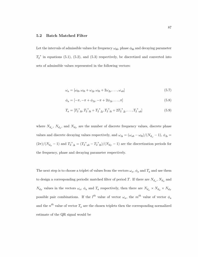
87
5.2 Batch Matched Filter
Let the intervals of admissible values for frequency ωbb, phase φbb and decaying parameter
T2∗ in equations (5.1), (5.2), and (5.3) respectively, be discretized and converted into
sets of admissible values represented in the following vectors:
ωa = [ωlb, ωlb + ω∆, ωlb + 2ω∆, . . . , ωub] (5.7)
φa = [−π,−π + φ∆,−π + 2φ∆, . . . , π] (5.8)
Ta = [T2∗lb, T2
∗lb + T2
∗∆, T2
∗lb + 2T2
∗∆, . . . , T2
∗ub] (5.9)
where Ndω , Ndφ , and NdT are the number of discrete frequency values, discrete phase
values and discrete decaying values respectively, and ω∆ = (ωub − ωlb)/(Ndω − 1), φ∆ =
(2π)/(Ndφ − 1) and T2∗
∆ = (T2∗ub − T2
∗lb)/(NdT − 1) are the discretization periods for
the frequency, phase and decaying parameter respectively.
The next step is to choose a triplet of values from the vectors ωa, φa and Ta and use them
to design a corresponding periodic matched filter of period T . If there are Ndω , Ndφ and
NdT values in the vectors ωa, φa and Ta respectively, then there are Ndω × Ndφ × NdT
possible pair combinations. If the lth value of vector ωa, the mth value of vector φa
and the nth value of vector Ta are the chosen triplets then the corresponding normalized
estimate of the QR signal would be
88
sl,m,n[k] =1
α(l,m, n)e(−|−T/2+k∆|/Ta(n))cos(ωa(l)(−T/2 + k∆) + φa(m)) (5.10)
for k = 0, 1, . . . , Ns − 1, where T is the length of the data acquisition window, Ns is the
number of discrete samples, ∆ = T/(Ns − 1) and the constant α(l,m, n) is the second
norm of the QR signal defined as,
α(l,m, n) =Ns−1∑k=0
[e(−|−T/2+k∆|/Ta(n))cos(ωa(l)(−T/2 + k∆) + φa(m))]2. (5.11)
Normalizing the filter by, α(l,m,m), the l2 norm is a necessary step to ensure that each
filter’s contribution to its inner product with the QR signal, had one been present, is
dependent on the match between them. Therefore, from Equation (4.12), the matched
filter, designed with white noise of unit variance in mind, for the above chosen QR signal
parameter values is the following periodic filter:
h[k] =Nm−1∑i=0
sl,m,n[k − iNs], (5.12)
for k = 0, 1, . . . , Nm × Ns − 1. After passing the received corrupted signal through the
filter with the above impulse response, the value of the Nm ×Nsth sample, which is
equivalent to the inner product of the received signal and the filter, is recorded and the
process is repeated for all different combinations of frequency ωbb, phase φbb and decaying
89
parameter T2∗ values. Repeating this procedure Ndω ×Ndφ×NdT times, for the different
possible triplets, leads to a vector Θ of values of length Ndω ×Ndφ ×NdT .
Θ = [θ1, . . . , θNdω×Ndφ×NdT] (5.13)
Finally the maximum value of the vector Θ is compared to a threshold value θthreshold
and the filter corresponding to this maximum is the chosen filter out of the batch.
Normalizing all the filters in the batch by their l2 norms increases the likelihood of the
chosen filter being the closest description of the QR signal present. If maximum value
of the vector Θ, is greater than the threshold then we conclude that a QR signal exists
within the corrupted signal, otherwise we conclude that the received signal is just noise.
Determining the value of θthreshold is still a matter that requires further work. There are
several possible ways of determining the value of θthreshold, one of which, is to collect
a measurement of the noise and use it to determine the value of θthreshold. The above
process of choosing the filter is equivalent to selecting the filter, hn[k], that maximizes
yn, the inner product of the filter with the received signal x[k], as follows
y = maxn
(yn) = maxn
(hn[k]Tx[k]
)= max
n
(|hn[k]||x[k]| cos γ
)
where γ is the angle between the received signal, x[k], and the filter hn[k]. The above
value is maximized when the value of the angle, γ, is zero, which corresponds to a value
of hn[k], equal to a scalar multiple of x[k]. For the selected filter, hn[k], to be x[k], the
received noise would have to zero and the QR signal present would have to be one of the
90
filters in the batch. If one assumes that the chosen filter out of the batch is equal to the
QR signal present, s[k], then the resulting signal to noise ratio defined in Equation (4.8)
is reduced to
ρ(s; s,Σ) =(s[k]T s[k])2
s[k]TΣs[k].
Had Σ been equal to the identity matrix, i.e. the noise present is white with unit variance,
the above signal to noise ratio would reduce to s[k]T s[k], which is the optimal signal to
noise ratio when the noise is white.
5.3 Batch Matched Filter versus Energy Detector, Unknown QR signal
This section compares the performance of the batch matched filter to the generic energy
detector, when the QR signal is unknown and no assumptions are placed on the noise,
which is the case in reality. The following subsection compares the performance of the
two detectors using simulation data. This subsection is followed by one that compares
their performance using experimental data collected in the laboratory.
For consistency, when comparing the batch matched filter to the energy detector (using
simulation and experimental data in the following two subsections) the batch matched
filter’s design parameters were fixed. The design of the filter assumes the presence of
thermal noise and therefore uses a Σ = I. The method gridded using the following
values, ωlb = 0, ωub = 40000π, ω∆ = 100π, φ∆ = .1, T ∗2 lb
= 300e − 6, T ∗2 ub
= 900e − 6
and T ∗2 ∆
= 100e−6. The above values lead to Ndω = 401, Ndφ = 63 and NdT = 7 in each
of the three dimensions, which corresponds to Ndω ×Ndφ ×NdT = 176841 filters in the
91
batch. The computational time of each one of those filters, which is an inner product, is
cheap and the process can be parallelized. The following sections will discuss the effect of
finer gridding on performance and will introduce a smarter adaptive gridding approach,
which reduces computational time.
5.3.1 Simulation Data
This section uses simulation data to compare the performance of the batch matched filter,
designed using the parameters at the beginning of the section, to the energy detector.
Six sets of simulation data of different frequencies, where the QR signal frequency and
the AM signal frequency are equal, were generated. The selected frequencies were 2.5, 5,
7.5, 10, 12.5 and 15 kHz. Each data set consisted of 100 experiments, where the received
signal is the sum of QR and AM, and 100 experiments, where the received signal consists
of only AM noise. Each experiment consisted of Nm = 5 trials strung in time, where
each is the average of 20 phase cycled echoes.
ROC plots were used to compare the performance of the batch matched filter to the
energy detector. Figures (5.6-5.11) compare the performance of the two detectors for
the different frequencies. The figures show that the batch matched filter outperforms
the energy detector for all cases. An outperformance by the batch matched filter was
expected since it was demonstrated in Chapter 4, when the QR signal was assumed to
be known.
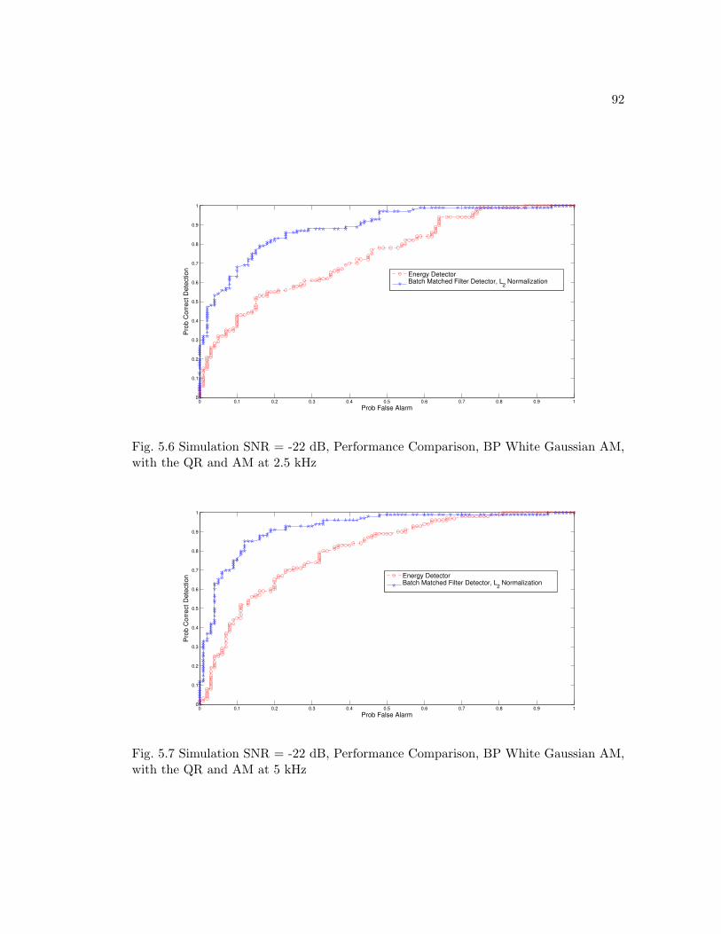
92
0 0.1 0.2 0.3 0.4 0.5 0.6 0.7 0.8 0.9 10
0.1
0.2
0.3
0.4
0.5
0.6
0.7
0.8
0.9
1
Pro
b C
orr
ect D
ete
ction
Prob False Alarm
Energy DetectorBatch Matched Filter Detector, L
2 Normalization
Fig. 5.6 Simulation SNR = -22 dB, Performance Comparison, BP White Gaussian AM,with the QR and AM at 2.5 kHz
0 0.1 0.2 0.3 0.4 0.5 0.6 0.7 0.8 0.9 10
0.1
0.2
0.3
0.4
0.5
0.6
0.7
0.8
0.9
1
Pro
b C
orr
ect D
ete
ction
Prob False Alarm
Energy DetectorBatch Matched Filter Detector, L
2 Normalization
Fig. 5.7 Simulation SNR = -22 dB, Performance Comparison, BP White Gaussian AM,with the QR and AM at 5 kHz
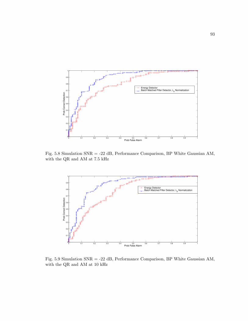
93
0 0.1 0.2 0.3 0.4 0.5 0.6 0.7 0.8 0.9 10
0.1
0.2
0.3
0.4
0.5
0.6
0.7
0.8
0.9
1
Pro
b C
orr
ect D
ete
ction
Prob False Alarm
Energy DetectorBatch Matched Filter Detector, L
2 Normalization
Fig. 5.8 Simulation SNR = -22 dB, Performance Comparison, BP White Gaussian AM,with the QR and AM at 7.5 kHz
0 0.1 0.2 0.3 0.4 0.5 0.6 0.7 0.8 0.9 10
0.1
0.2
0.3
0.4
0.5
0.6
0.7
0.8
0.9
1
Pro
b C
orr
ect D
ete
ction
Prob False Alarm
Energy DetectorBatch Matched Filter Detector, L
2 Normalization
Fig. 5.9 Simulation SNR = -22 dB, Performance Comparison, BP White Gaussian AM,with the QR and AM at 10 kHz
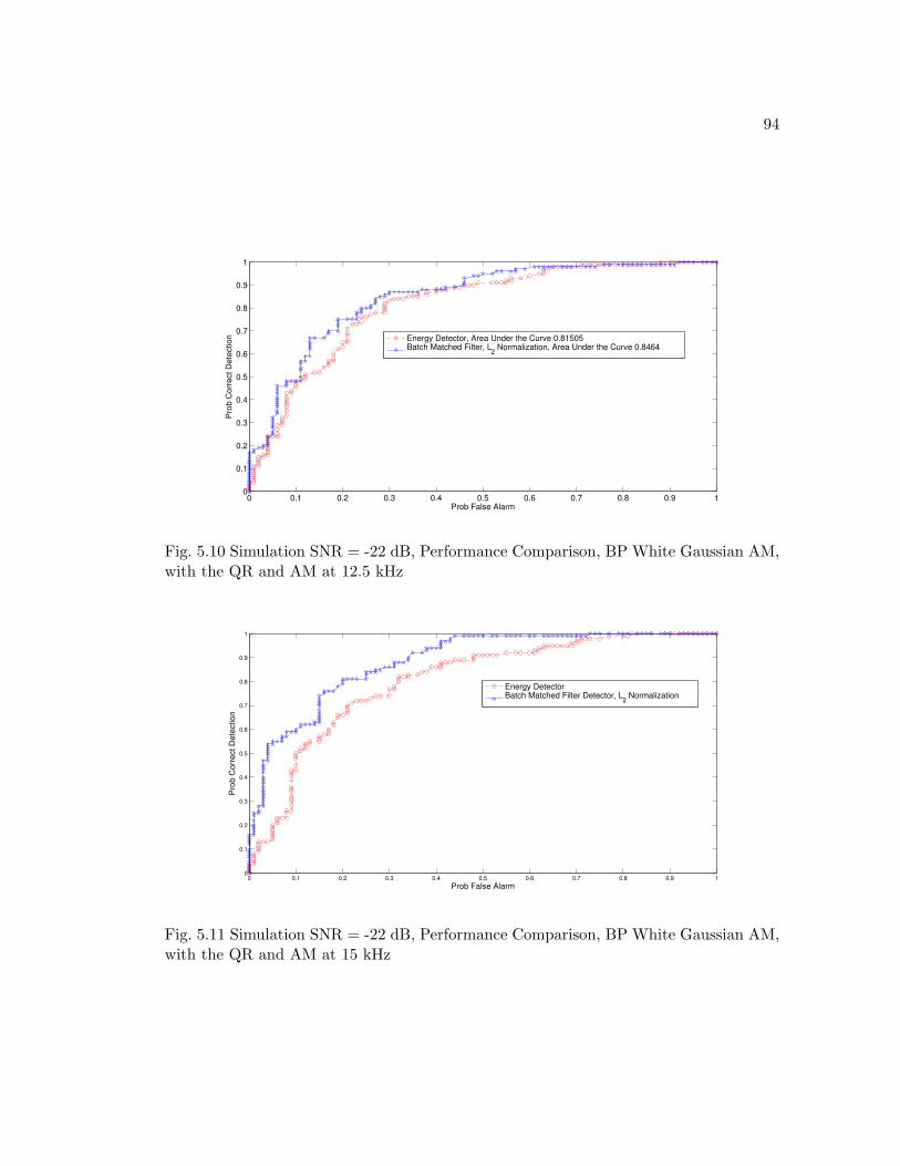
94
0 0.1 0.2 0.3 0.4 0.5 0.6 0.7 0.8 0.9 10
0.1
0.2
0.3
0.4
0.5
0.6
0.7
0.8
0.9
1
Pro
b C
orr
ect D
ete
ction
Prob False Alarm
Energy Detector, Area Under the Curve 0.81505Batch Matched Filter, L
2 Normalization, Area Under the Curve 0.8464
Fig. 5.10 Simulation SNR = -22 dB, Performance Comparison, BP White Gaussian AM,with the QR and AM at 12.5 kHz
0 0.1 0.2 0.3 0.4 0.5 0.6 0.7 0.8 0.9 10
0.1
0.2
0.3
0.4
0.5
0.6
0.7
0.8
0.9
1
Pro
b C
orr
ect D
ete
ction
Prob False Alarm
Energy DetectorBatch Matched Filter Detector, L
2 Normalization
Fig. 5.11 Simulation SNR = -22 dB, Performance Comparison, BP White Gaussian AM,with the QR and AM at 15 kHz
95
5.3.2 Experimental Data
This section uses experimental data to compare the performance of the batch matched
filter, designed using the parameters at the beginning of the section, to the energy
detector. Four sets of experiment data of different frequencies, where the QR signal
baseband frequency and AM signal baseband frequency are equal, were collected. The
four sets, which will be referred to as A, B, C and D have frequencies 6.25, 10, 8 and 12.5
kHz respectively. Each set consisted of 100 experiments, where the received signal is the
sum of a QR signal an AM signal and thermal noise, and the another 100 experiments,
where the received signal is the sum of an AM signal and thermal noise. Each experiment
consists of Nm = 5 trials strung in time, where each is the average of 20 phase-cycled
echoes.
ROC plots were used to compare the performance of the two detectors for the different
experimental sets. These ROC plots are shown in Figures (5.12)-(5.15) for experiments
A-D respectively. The batch matched filter with the gridding parameters mentioned at
the beginning of the section, is represented by the blue curve in the figures. The green
represents a batch matched filter with different gridding parameters, than the ones above,
and will be discussed in the following section. The figures show that the batch matched
filter outperforms the energy detector in all cases.
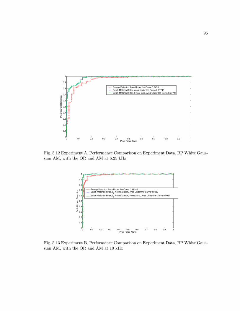
96
0 0.1 0.2 0.3 0.4 0.5 0.6 0.7 0.8 0.9 10
0.1
0.2
0.3
0.4
0.5
0.6
0.7
0.8
0.9
1
Pro
b C
orr
ect D
ete
ction
Prob False Alarm
Energy Detector, Area Under the Curve 0.9455
Batch Matched Filter, Area Under the Curve 0.97745
Batch Matched Filter, Finest Grid, Area Under the Curve 0.97745
Fig. 5.12 Experiment A, Performance Comparison on Experiment Data, BP White Gaus-sian AM, with the QR and AM at 6.25 kHz
0 0.1 0.2 0.3 0.4 0.5 0.6 0.7 0.8 0.9 10
0.1
0.2
0.3
0.4
0.5
0.6
0.7
0.8
0.9
1
Pro
b C
orr
ect D
ete
ction
Prob False Alarm
Energy Detector, Area Under the Curve 0.98385Batch Matched Filter, L
2 Normalization, Area Under the Curve 0.9987
Batch Matched Filter, L2 Normalization, Finest Grid, Area Under the Curve 0.9987
Fig. 5.13 Experiment B, Performance Comparison on Experiment Data, BP White Gaus-sian AM, with the QR and AM at 10 kHz
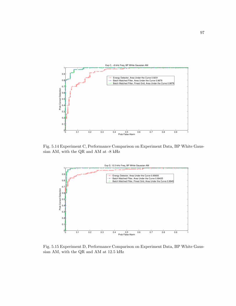
97
0 0.1 0.2 0.3 0.4 0.5 0.6 0.7 0.8 0.9 10
0.1
0.2
0.3
0.4
0.5
0.6
0.7
0.8
0.9
1
Pro
b C
orr
ect D
ete
ction
Prob False Alarm
Exp C, −8 kHz Freq, BP White Gaussian AM
Energy Detector, Area Under the Curve 0.9231
Batch Matched Filter, Area Under the Curve 0.9878
Batch Matched Filter, Finest Grid, Area Under the Curve 0.9878
Fig. 5.14 Experiment C, Performance Comparison on Experiment Data, BP White Gaus-sian AM, with the QR and AM at -8 kHz
0 0.1 0.2 0.3 0.4 0.5 0.6 0.7 0.8 0.9 10
0.1
0.2
0.3
0.4
0.5
0.6
0.7
0.8
0.9
1
Pro
b C
orr
ect D
ete
ction
Prob False Alarm
Exp D, 12.5 kHz Freq, BP White Gaussian AM
Energy Detector, Area Under the Curve 0.95655
Batch Matched Filter, Area Under the Curve 0.99435
Batch Matched Filter, Finest Grid, Area Under the Curve 0.9945
Fig. 5.15 Experiment D, Performance Comparison on Experiment Data, BP White Gaus-sian AM, with the QR and AM at 12.5 kHz
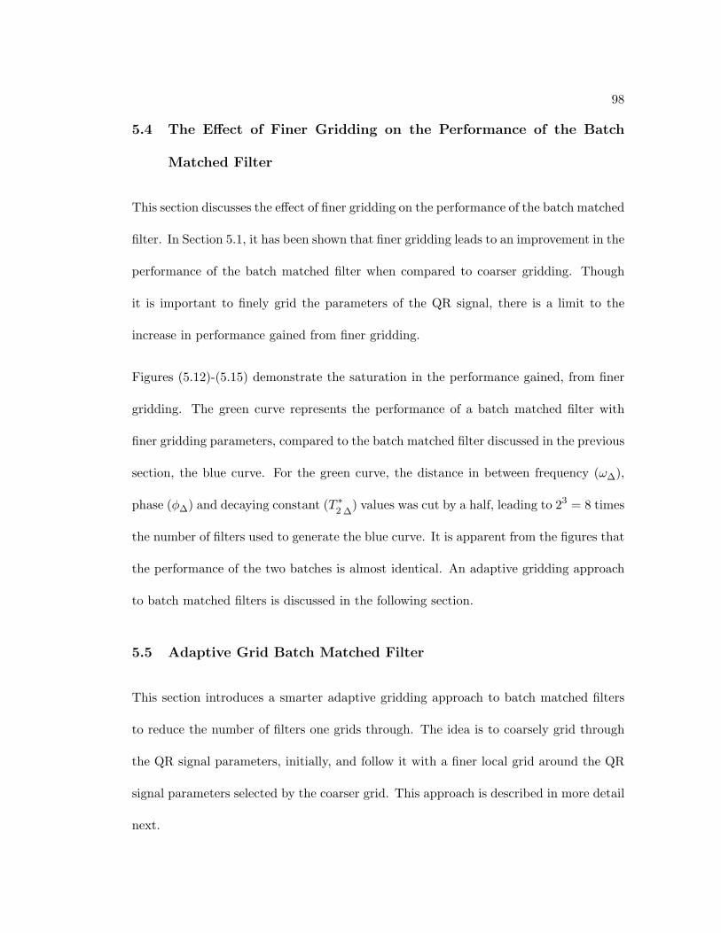
98
5.4 The Effect of Finer Gridding on the Performance of the Batch
Matched Filter
This section discusses the effect of finer gridding on the performance of the batch matched
filter. In Section 5.1, it has been shown that finer gridding leads to an improvement in the
performance of the batch matched filter when compared to coarser gridding. Though
it is important to finely grid the parameters of the QR signal, there is a limit to the
increase in performance gained from finer gridding.
Figures (5.12)-(5.15) demonstrate the saturation in the performance gained, from finer
gridding. The green curve represents the performance of a batch matched filter with
finer gridding parameters, compared to the batch matched filter discussed in the previous
section, the blue curve. For the green curve, the distance in between frequency (ω∆),
phase (φ∆) and decaying constant (T ∗2 ∆
) values was cut by a half, leading to 23 = 8 times
the number of filters used to generate the blue curve. It is apparent from the figures that
the performance of the two batches is almost identical. An adaptive gridding approach
to batch matched filters is discussed in the following section.
5.5 Adaptive Grid Batch Matched Filter
This section introduces a smarter adaptive gridding approach to batch matched filters
to reduce the number of filters one grids through. The idea is to coarsely grid through
the QR signal parameters, initially, and follow it with a finer local grid around the QR
signal parameters selected by the coarser grid. This approach is described in more detail
next.
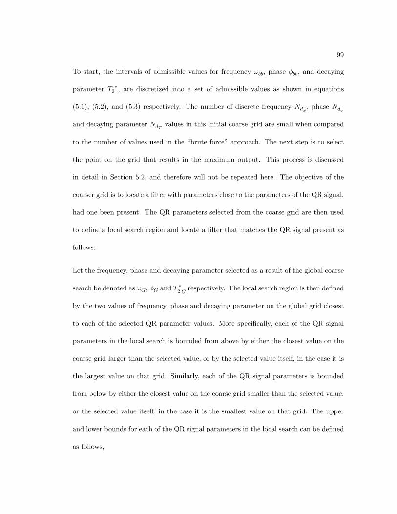
99
To start, the intervals of admissible values for frequency ωbb, phase φbb, and decaying
parameter T2∗, are discretized into a set of admissible values as shown in equations
(5.1), (5.2), and (5.3) respectively. The number of discrete frequency Ndω , phase Ndφ
and decaying parameter NdT values in this initial coarse grid are small when compared
to the number of values used in the “brute force” approach. The next step is to select
the point on the grid that results in the maximum output. This process is discussed
in detail in Section 5.2, and therefore will not be repeated here. The objective of the
coarser grid is to locate a filter with parameters close to the parameters of the QR signal,
had one been present. The QR parameters selected from the coarse grid are then used
to define a local search region and locate a filter that matches the QR signal present as
follows.
Let the frequency, phase and decaying parameter selected as a result of the global coarse
search be denoted as ωG, φG and T ∗2 G
respectively. The local search region is then defined
by the two values of frequency, phase and decaying parameter on the global grid closest
to each of the selected QR parameter values. More specifically, each of the QR signal
parameters in the local search is bounded from above by either the closest value on the
coarse grid larger than the selected value, or by the selected value itself, in the case it is
the largest value on that grid. Similarly, each of the QR signal parameters is bounded
from below by either the closest value on the coarse grid smaller than the selected value,
or the selected value itself, in the case it is the smallest value on that grid. The upper
and lower bounds for each of the QR signal parameters in the local search can be defined
as follows,
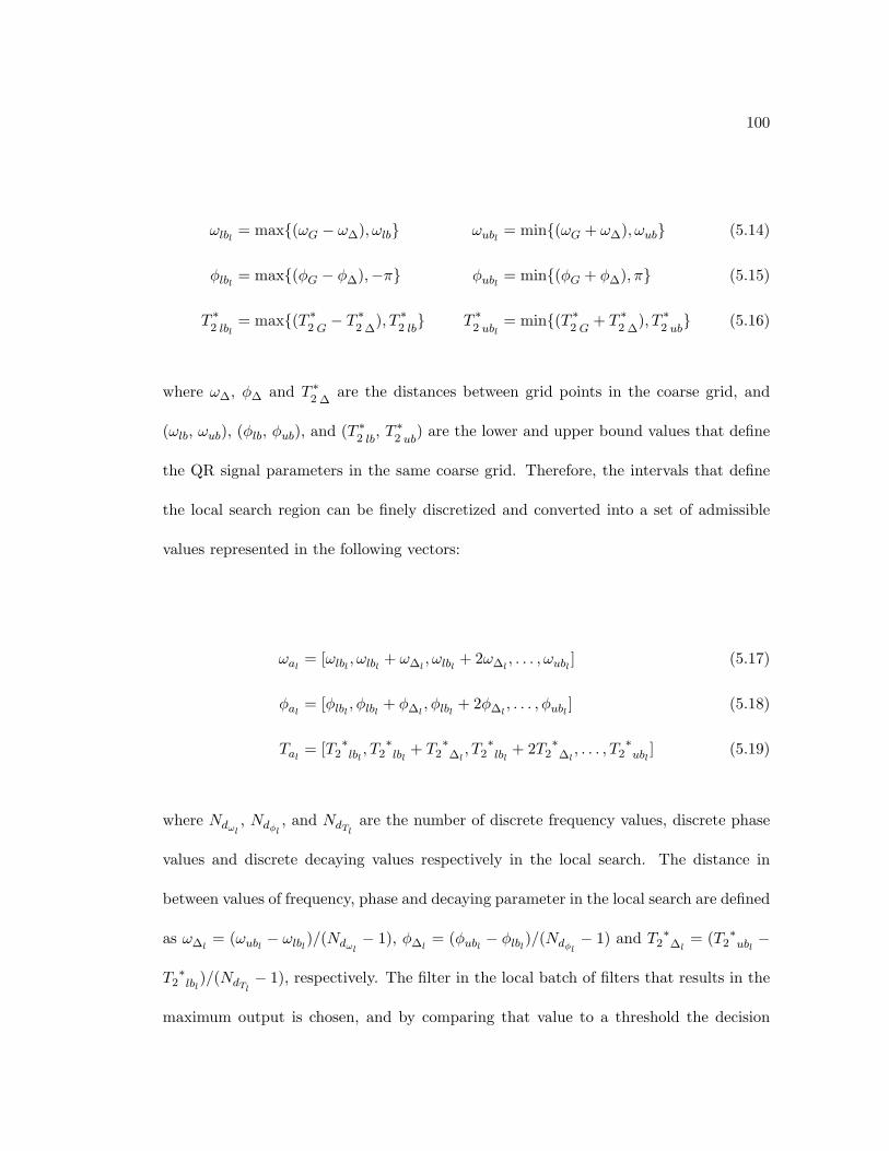
100
ωlbl = max{(ωG − ω∆), ωlb} ωubl = min{(ωG + ω∆), ωub} (5.14)
φlbl = max{(φG − φ∆),−π} φubl = min{(φG + φ∆), π} (5.15)
T ∗2 lbl
= max{(T ∗2 G− T ∗
2 ∆), T ∗
2 lb} T ∗
2 ubl= min{(T ∗
2 G+ T ∗
2 ∆), T ∗
2 ub} (5.16)
where ω∆, φ∆ and T ∗2 ∆
are the distances between grid points in the coarse grid, and
(ωlb, ωub), (φlb, φub), and (T ∗2 lb
, T ∗2 ub
) are the lower and upper bound values that define
the QR signal parameters in the same coarse grid. Therefore, the intervals that define
the local search region can be finely discretized and converted into a set of admissible
values represented in the following vectors:
ωal = [ωlbl , ωlbl + ω∆l, ωlbl + 2ω∆l
, . . . , ωubl ] (5.17)
φal = [φlbl , φlbl + φ∆l, φlbl + 2φ∆l
, . . . , φubl ] (5.18)
Tal = [T2∗lbl, T2∗lbl
+ T2∗
∆l, T2∗lbl
+ 2T2∗
∆l, . . . , T2
∗ubl
] (5.19)
where Ndωl, Ndφl
, and NdTlare the number of discrete frequency values, discrete phase
values and discrete decaying values respectively in the local search. The distance in
between values of frequency, phase and decaying parameter in the local search are defined
as ω∆l= (ωubl − ωlbl)/(Ndωl
− 1), φ∆l= (φubl − φlbl)/(Ndφl
− 1) and T2∗
∆l= (T2
∗ubl−
T2∗lbl
)/(NdTl− 1), respectively. The filter in the local batch of filters that results in the
maximum output is chosen, and by comparing that value to a threshold the decision
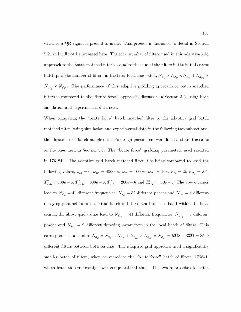
101
whether a QR signal is present is made. This process is discussed in detail in Section
5.2, and will not be repeated here. The total number of filters used in this adaptive grid
approach to the batch matched filter is equal to the sum of the filters in the initial coarse
batch plus the number of filters in the later local fine batch, Ndω ×Ndφ ×NdT +Ndωl×
Ndφl× NdTl
. The performance of this adaptive gridding approach to batch matched
filters is compared to the “brute force” approach, discussed in Section 5.2, using both
simulation and experimental data next.
When comparing the “brute force” batch matched filter to the adaptive grid batch
matched filter (using simulation and experimental data in the following two subsections)
the “brute force” batch matched filter’s design parameters were fixed and are the same
as the ones used in Section 5.3. The “brute force” gridding parameters used resulted
in 176, 841. The adaptive grid batch matched filter it is being compared to used the
following values, ωlb = 0, ωub = 40000π, ω∆ = 1000π, ω∆l= 50π, φ∆ = .2, φ∆l
= .05,
T ∗2 lb
= 300e− 6, T ∗2 ub
= 900e− 6, T ∗2 ∆
= 200e− 6 and T ∗2 ∆l
= 50e− 6. The above values
lead to Ndω = 41 different frequencies, Ndφ = 32 different phases and NdT = 4 different
decaying parameters in the initial batch of filters. On the other hand within the local
search, the above grid values lead to Ndωl= 41 different frequencies, Ndφl
= 9 different
phases and NdTl= 9 different decaying parameters in the local batch of filters. This
corresponds to a total of Ndω ×Ndφ ×NdT +Ndωl×Ndφl
×NdTl= 5248 + 3321 = 8569
different filters between both batches. The adaptive grid approach used a significantly
smaller batch of filters, when compared to the “brute force” batch of filters, 176841,
which leads to significantly lower computational time. The two approaches to batch
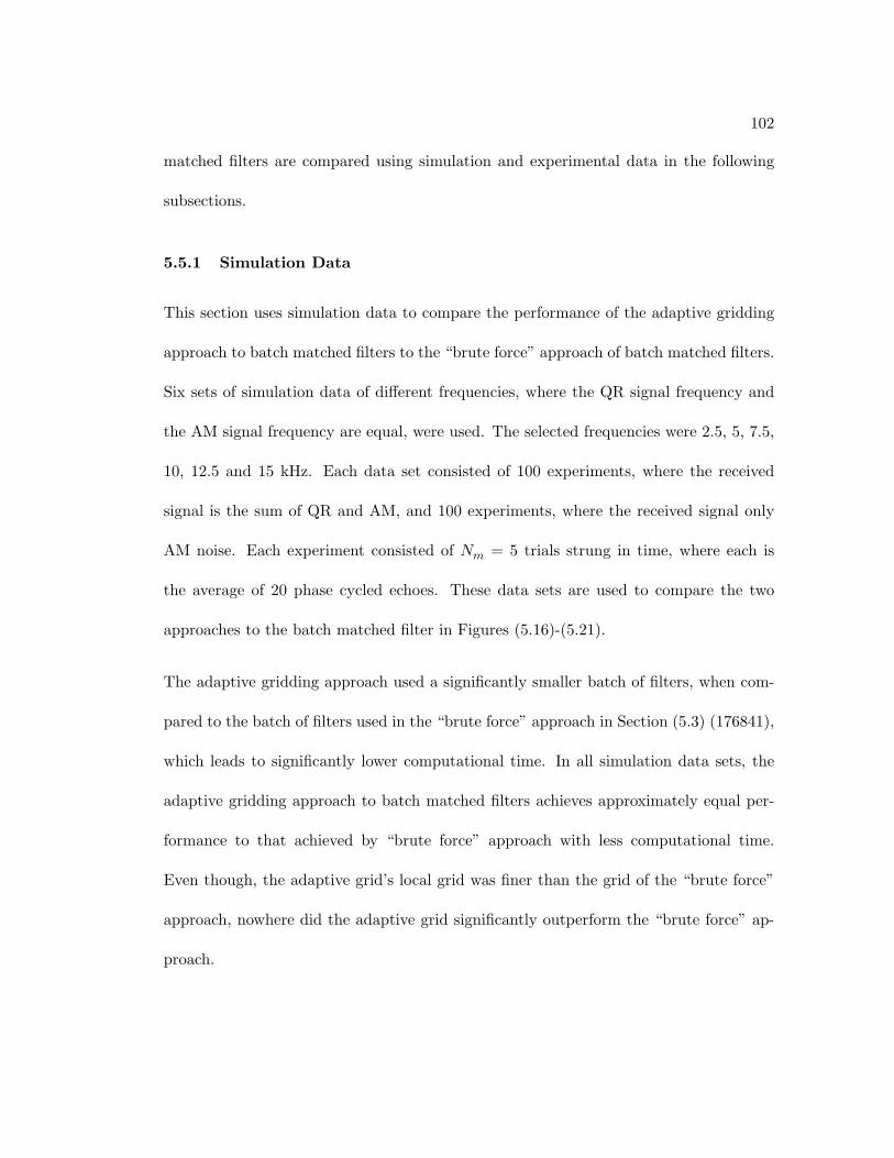
102
matched filters are compared using simulation and experimental data in the following
subsections.
5.5.1 Simulation Data
This section uses simulation data to compare the performance of the adaptive gridding
approach to batch matched filters to the “brute force” approach of batch matched filters.
Six sets of simulation data of different frequencies, where the QR signal frequency and
the AM signal frequency are equal, were used. The selected frequencies were 2.5, 5, 7.5,
10, 12.5 and 15 kHz. Each data set consisted of 100 experiments, where the received
signal is the sum of QR and AM, and 100 experiments, where the received signal only
AM noise. Each experiment consisted of Nm = 5 trials strung in time, where each is
the average of 20 phase cycled echoes. These data sets are used to compare the two
approaches to the batch matched filter in Figures (5.16)-(5.21).
The adaptive gridding approach used a significantly smaller batch of filters, when com-
pared to the batch of filters used in the “brute force” approach in Section (5.3) (176841),
which leads to significantly lower computational time. In all simulation data sets, the
adaptive gridding approach to batch matched filters achieves approximately equal per-
formance to that achieved by “brute force” approach with less computational time.
Even though, the adaptive grid’s local grid was finer than the grid of the “brute force”
approach, nowhere did the adaptive grid significantly outperform the “brute force” ap-
proach.
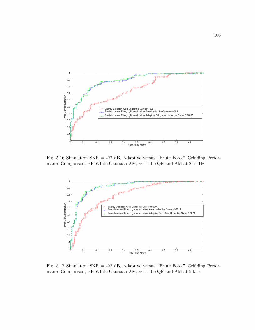
103
0 0.1 0.2 0.3 0.4 0.5 0.6 0.7 0.8 0.9 10
0.1
0.2
0.3
0.4
0.5
0.6
0.7
0.8
0.9
1
Pro
b C
orr
ect D
ete
ction
Prob False Alarm
Energy Detector, Area Under the Curve 0.7396Batch Matched Filter, L
2 Normalization, Area Under the Curve 0.88555
Batch Matched Filter, L2 Normalization, Adaptive Grid, Area Under the Curve 0.88825
Fig. 5.16 Simulation SNR = -22 dB, Adaptive versus “Brute Force” Gridding Perfor-mance Comparison, BP White Gaussian AM, with the QR and AM at 2.5 kHz
0 0.1 0.2 0.3 0.4 0.5 0.6 0.7 0.8 0.9 10
0.1
0.2
0.3
0.4
0.5
0.6
0.7
0.8
0.9
1
Pro
b C
orr
ect D
ete
ction
Prob False Alarm
Energy Detector, Area Under the Curve 0.80095Batch Matched Filter, L
2 Normalization, Area Under the Curve 0.92015
Batch Matched Filter, L2 Normalization, Adaptive Grid, Area Under the Curve 0.9226
Fig. 5.17 Simulation SNR = -22 dB, Adaptive versus “Brute Force” Gridding Perfor-mance Comparison, BP White Gaussian AM, with the QR and AM at 5 kHz
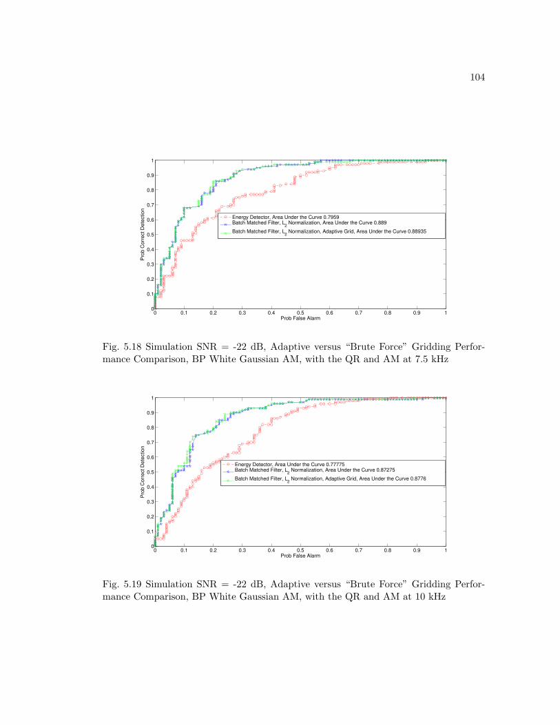
104
0 0.1 0.2 0.3 0.4 0.5 0.6 0.7 0.8 0.9 10
0.1
0.2
0.3
0.4
0.5
0.6
0.7
0.8
0.9
1
Pro
b C
orr
ect D
ete
ction
Prob False Alarm
Energy Detector, Area Under the Curve 0.7959Batch Matched Filter, L
2 Normalization, Area Under the Curve 0.889
Batch Matched Filter, L2 Normalization, Adaptive Grid, Area Under the Curve 0.88935
Fig. 5.18 Simulation SNR = -22 dB, Adaptive versus “Brute Force” Gridding Perfor-mance Comparison, BP White Gaussian AM, with the QR and AM at 7.5 kHz
0 0.1 0.2 0.3 0.4 0.5 0.6 0.7 0.8 0.9 10
0.1
0.2
0.3
0.4
0.5
0.6
0.7
0.8
0.9
1
Pro
b C
orr
ect D
ete
ction
Prob False Alarm
Energy Detector, Area Under the Curve 0.77775Batch Matched Filter, L
2 Normalization, Area Under the Curve 0.87275
Batch Matched Filter, L2 Normalization, Adaptive Grid, Area Under the Curve 0.8776
Fig. 5.19 Simulation SNR = -22 dB, Adaptive versus “Brute Force” Gridding Perfor-mance Comparison, BP White Gaussian AM, with the QR and AM at 10 kHz
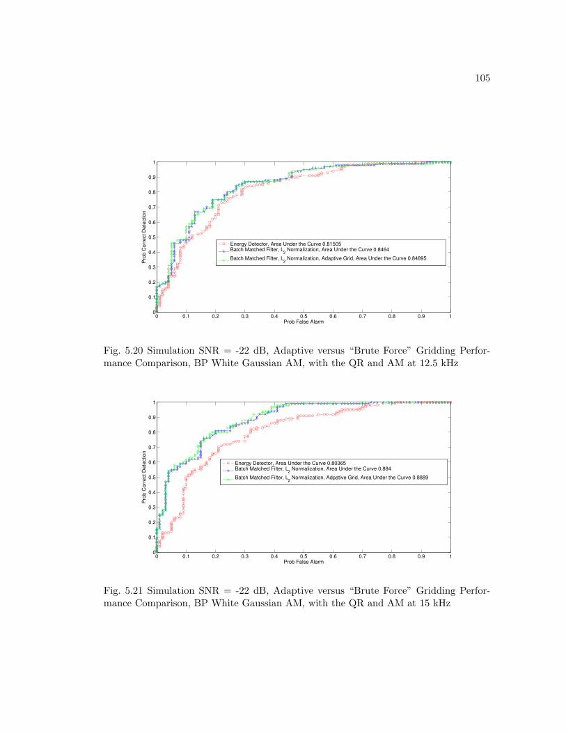
105
0 0.1 0.2 0.3 0.4 0.5 0.6 0.7 0.8 0.9 10
0.1
0.2
0.3
0.4
0.5
0.6
0.7
0.8
0.9
1
Pro
b C
orr
ect D
ete
ction
Prob False Alarm
Energy Detector, Area Under the Curve 0.81505Batch Matched Filter, L
2 Normalization, Area Under the Curve 0.8464
Batch Matched Filter, L2 Normalization, Adaptive Grid, Area Under the Curve 0.84895
Fig. 5.20 Simulation SNR = -22 dB, Adaptive versus “Brute Force” Gridding Perfor-mance Comparison, BP White Gaussian AM, with the QR and AM at 12.5 kHz
0 0.1 0.2 0.3 0.4 0.5 0.6 0.7 0.8 0.9 10
0.1
0.2
0.3
0.4
0.5
0.6
0.7
0.8
0.9
1
Pro
b C
orr
ect D
ete
ction
Prob False Alarm
Energy Detector, Area Under the Curve 0.80365Batch Matched Filter, L
2 Normalization, Area Under the Curve 0.884
Batch Matched Filter, L2 Normalization, Adpative Grid, Area Under the Curve 0.8889
Fig. 5.21 Simulation SNR = -22 dB, Adaptive versus “Brute Force” Gridding Perfor-mance Comparison, BP White Gaussian AM, with the QR and AM at 15 kHz
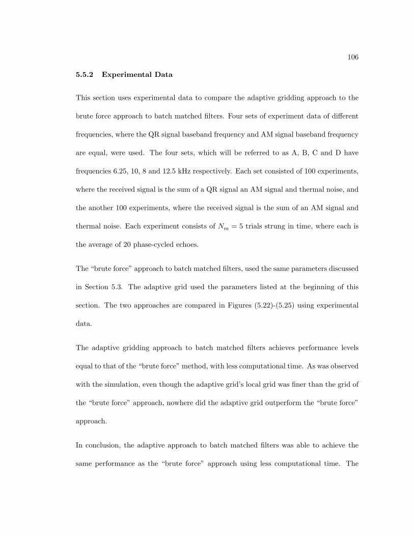
106
5.5.2 Experimental Data
This section uses experimental data to compare the adaptive gridding approach to the
brute force approach to batch matched filters. Four sets of experiment data of different
frequencies, where the QR signal baseband frequency and AM signal baseband frequency
are equal, were used. The four sets, which will be referred to as A, B, C and D have
frequencies 6.25, 10, 8 and 12.5 kHz respectively. Each set consisted of 100 experiments,
where the received signal is the sum of a QR signal an AM signal and thermal noise, and
the another 100 experiments, where the received signal is the sum of an AM signal and
thermal noise. Each experiment consists of Nm = 5 trials strung in time, where each is
the average of 20 phase-cycled echoes.
The “brute force” approach to batch matched filters, used the same parameters discussed
in Section 5.3. The adaptive grid used the parameters listed at the beginning of this
section. The two approaches are compared in Figures (5.22)-(5.25) using experimental
data.
The adaptive gridding approach to batch matched filters achieves performance levels
equal to that of the “brute force” method, with less computational time. As was observed
with the simulation, even though the adaptive grid’s local grid was finer than the grid of
the “brute force” approach, nowhere did the adaptive grid outperform the “brute force”
approach.
In conclusion, the adaptive approach to batch matched filters was able to achieve the
same performance as the “brute force” approach using less computational time. The
107
0 0.1 0.2 0.3 0.4 0.5 0.6 0.7 0.8 0.9 10
0.1
0.2
0.3
0.4
0.5
0.6
0.7
0.8
0.9
1
Pro
b C
orr
ect D
ete
ction
Prob False Alarm
Energy Detector, Area Under the Curve 0.9455Batch Matched Filter, L
2 Normalization, Area Under the Curve 0.97745
Batch Matched Filter, L2 Normalization, Adaptive Grid, Area Under the Curve 0.977
Fig. 5.22 Experiment A, Adaptive versus “Brute Force” Gridding Performance Com-parison on Experiment Data, BP White Gaussian AM, with the QR and AM at 6.25kHz
0 0.1 0.2 0.3 0.4 0.5 0.6 0.7 0.8 0.9 10
0.1
0.2
0.3
0.4
0.5
0.6
0.7
0.8
0.9
1
Pro
b C
orr
ect D
ete
ction
Prob False Alarm
Energy Detector, Area Under the Curve 0.98385Batch Matched Filter, L
2 Normalization, Area Under the Curve 0.9987
Batch Matched Filter, L2 Normalization, Adpative Grid, Area Under the Curve 0.9989
Fig. 5.23 Experiment B, Adaptive versus “Brute Force” Gridding Performance Com-parison on Experiment Data, BP White Gaussian AM, with the QR and AM at 10kHz
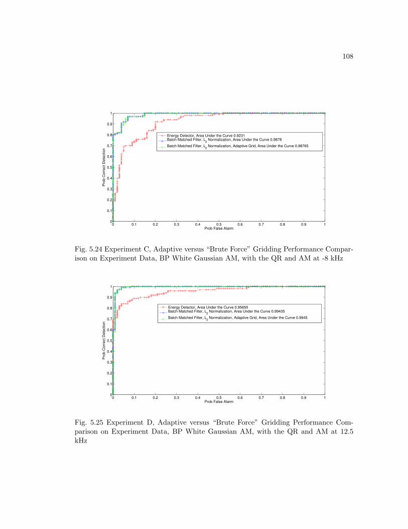
108
0 0.1 0.2 0.3 0.4 0.5 0.6 0.7 0.8 0.9 10
0.1
0.2
0.3
0.4
0.5
0.6
0.7
0.8
0.9
1
Pro
b C
orr
ect D
ete
ction
Prob False Alarm
Energy Detector, Area Under the Curve 0.9231Batch Matched Filter, L
2 Normalization, Area Under the Curve 0.9878
Batch Matched Filter, L2 Normalization, Adaptive Grid, Area Under the Curve 0.98765
Fig. 5.24 Experiment C, Adaptive versus “Brute Force” Gridding Performance Compar-ison on Experiment Data, BP White Gaussian AM, with the QR and AM at -8 kHz
0 0.1 0.2 0.3 0.4 0.5 0.6 0.7 0.8 0.9 10
0.1
0.2
0.3
0.4
0.5
0.6
0.7
0.8
0.9
1
Pro
b C
orr
ect D
ete
ction
Prob False Alarm
Energy Detector, Area Under the Curve 0.95655Batch Matched Filter, L
2 Normalization, Area Under the Curve 0.99435
Batch Matched Filter, L2 Normalization, Adaptive Grid, Area Under the Curve 0.9945
Fig. 5.25 Experiment D, Adaptive versus “Brute Force” Gridding Performance Com-parison on Experiment Data, BP White Gaussian AM, with the QR and AM at 12.5kHz
109
following chapters will use the “brute force” approach to matched filters with a fine grid,
unless specified otherwise. The following section discusses an alternative approach to
the maximum output used in making a QR detection decision.
5.6 Alternative Detection Decisions
This section investigates the effect of using several filter outputs, to determine the pres-
ence of a QR signal, on performance. The idea is to base the QR detection decision not
only on the maximum output (out of the batch of filters) but also the output of a group
of surrounding filters, with QR parameters close to the parameters of the filter with the
maximum output. The goal is to decrease the false alarm rate for a fixed probability of
correct detection by using several output values versus one.
We chose to average, using equal weights, the maximum output value of the batch
matched filter and the output of a group of six filters, that surround the filter resulting
in the maximum output. The average output value is then compared to a threshold to
determine the presence of a QR signal. The group of filters used are chosen as follows.
Let ωmax, φmax, and T2∗max denote the frequency, phase and decaying parameter re-
spectively of the filter resulting in the maximum output and ω∆, φ∆ and T2∗
∆ denote
the distance between grid points in the frequency, phase and decaying parameter dimen-
sions respectively. In which case the group of filters would have the following QR signal
parameters:
1. φ = φmax, T2∗ = T2
∗max, ω∗ = ωmax − αω∆
2. φ = φmax, T2∗ = T2
∗max, ω∗ = ωmax + αω∆
110
3. ω∗ = ωmax, T2∗ = T2
∗max, φ = φmax − αφ∆
4. ω∗ = ωmax, T2∗ = T2
∗max, φ = φmax + αφ∆
5. ω∗ = ωmax, φ = φmax T2∗ = T2
∗max − αT2
∗∆
6. ω∗ = ωmax, φ = φmax T2∗ = T2
∗max + αT2
∗∆
where α is a multiple that can be varied to vary the distance between the QR signal
parameters of the filters. Using the gridding parameters described in Section 5.3, the
above average thresholding method was applied for the following three different values
of α, 0.5, 1, and 2. Both simulation and experimental data sets were used to compare
the performance of this method to the simple maximum output decision method used
in Section 5.3. The ROC curves generated using the different data sets are shown in
Figures (5.26)-(5.35), starting with the simulation data.
From comparing the ROC plots in the figures, it is apparent that using the average
output of a group of filters, does not improve the performance resulting from using the
maximum output only as a decision criteria. This means that the correlation between an
AM signal and the filter (resulting in the maximum output) decreases almost in the same
amount as the correlation between a QR signal and the filter (resulting in the maximum
output) as the filter parameters are varied within a local region surround the maximum
output filter. Therefore, due to the lack of improvement in performance, when using
the average output, and the simplicity of the maximum output approach, the decision
criteria that will be used in the rest of the thesis will be the maximum output value.
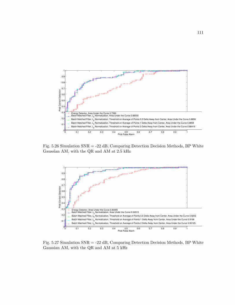
111
0 0.1 0.2 0.3 0.4 0.5 0.6 0.7 0.8 0.9 10
0.1
0.2
0.3
0.4
0.5
0.6
0.7
0.8
0.9
1
Pro
b C
orr
ect D
ete
ction
Prob False Alarm
Energy Detector, Area Under the Curve 0.7396Batch Matched Filter, L
2 Normalization, Area Under the Curve 0.88555
Batch Matched Filter, L2 Normalization, Threshold on Average of Points 0.5 Delta Away from Center, Area Under the Curve 0.8856
Batch Matched Filter, L2 Normalization, Threshold on Average of Points 1 Delta Away from Center, Area Under the Curve 0.8858
Batch Matched Filter, L2 Normalization, Threshold on Average of Points 2 Delta Away from Center, Area Under the Curve 0.88415
Fig. 5.26 Simulation SNR = -22 dB, Comparing Detection Decision Methods, BP WhiteGaussian AM, with the QR and AM at 2.5 kHz
0 0.1 0.2 0.3 0.4 0.5 0.6 0.7 0.8 0.9 10
0.1
0.2
0.3
0.4
0.5
0.6
0.7
0.8
0.9
1
Pro
b C
orr
ect D
ete
ction
Prob False Alarm
Energy Detector, Area Under the Curve 0.80095Batch Matched Filter, L
2 Normalization, Area Under the Curve 0.92015
Batch Matched Filter, L2 Normalization, Threshold on Average of Points 0.5 Delta Away from Center, Area Under the Curve 0.9202
Batch Matched Filter, L2 Normalization, Threshold on Average of Points 1 Delta Away from Center, Area Under the Curve 0.9198
Batch Matched Filter, L2 Normalization, Threshold on Average of Points 2 Delta Away from Center, Area Under the Curve 0.92125
Fig. 5.27 Simulation SNR = -22 dB, Comparing Detection Decision Methods, BP WhiteGaussian AM, with the QR and AM at 5 kHz
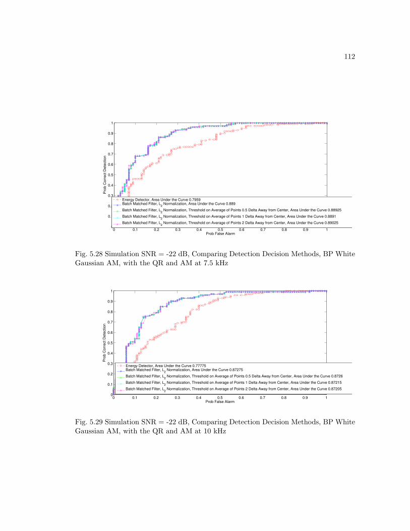
112
0 0.1 0.2 0.3 0.4 0.5 0.6 0.7 0.8 0.9 10
0.1
0.2
0.3
0.4
0.5
0.6
0.7
0.8
0.9
1
Pro
b C
orr
ect D
ete
ction
Prob False Alarm
Energy Detector, Area Under the Curve 0.7959Batch Matched Filter, L
2 Normalization, Area Under the Curve 0.889
Batch Matched Filter, L2 Normalization, Threshold on Average of Points 0.5 Delta Away from Center, Area Under the Curve 0.88925
Batch Matched Filter, L2 Normalization, Threshold on Average of Points 1 Delta Away from Center, Area Under the Curve 0.8891
Batch Matched Filter, L2 Normalization, Threshold on Average of Points 2 Delta Away from Center, Area Under the Curve 0.89025
Fig. 5.28 Simulation SNR = -22 dB, Comparing Detection Decision Methods, BP WhiteGaussian AM, with the QR and AM at 7.5 kHz
0 0.1 0.2 0.3 0.4 0.5 0.6 0.7 0.8 0.9 10
0.1
0.2
0.3
0.4
0.5
0.6
0.7
0.8
0.9
1
Pro
b C
orr
ect D
ete
ction
Prob False Alarm
Energy Detector, Area Under the Curve 0.77775Batch Matched Filter, L
2 Normalization, Area Under the Curve 0.87275
Batch Matched Filter, L2 Normalization, Threshold on Average of Points 0.5 Delta Away from Center, Area Under the Curve 0.8726
Batch Matched Filter, L2 Normalization, Threshold on Average of Points 1 Delta Away from Center, Area Under the Curve 0.87215
Batch Matched Filter, L2 Normalization, Threshold on Average of Points 2 Delta Away from Center, Area Under the Curve 0.87205
Fig. 5.29 Simulation SNR = -22 dB, Comparing Detection Decision Methods, BP WhiteGaussian AM, with the QR and AM at 10 kHz
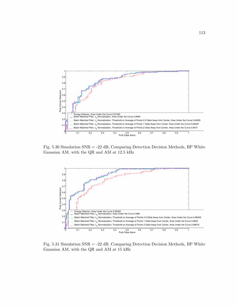
113
0 0.1 0.2 0.3 0.4 0.5 0.6 0.7 0.8 0.9 10
0.1
0.2
0.3
0.4
0.5
0.6
0.7
0.8
0.9
1
Pro
b C
orr
ect D
ete
ction
Prob False Alarm
Energy Detector, Area Under the Curve 0.81505Batch Matched Filter, L
2 Normalization, Area Under the Curve 0.8464
Batch Matched Filter, L2 Normalization, Threshold on Average of Points 0.5 Delta Away from Center, Area Under the Curve 0.84595
Batch Matched Filter, L2 Normalization, Threshold on Average of Points 1 Delta Away from Center, Area Under the Curve 0.84635
Batch Matched Filter, L2 Normalization, Threshold on Average of Points 2 Delta Away from Center, Area Under the Curve 0.8473
Fig. 5.30 Simulation SNR = -22 dB, Comparing Detection Decision Methods, BP WhiteGaussian AM, with the QR and AM at 12.5 kHz
0 0.1 0.2 0.3 0.4 0.5 0.6 0.7 0.8 0.9 10
0.1
0.2
0.3
0.4
0.5
0.6
0.7
0.8
0.9
1
Pro
b C
orr
ect D
ete
ction
Prob False Alarm
Energy Detector, Area Under the Curve 0.80365Batch Matched Filter, L
2 Normalization, Area Under the Curve 0.884
Batch Matched Filter, L2 Normalization, Threshold on Average of Points 0.5 Delta Away from Center, Area Under the Curve 0.88405
Batch Matched Filter, L2 Normalization, Threshold on Average of Points 1 Delta Away from Center, Area Under the Curve 0.8844
Batch Matched Filter, L2 Normalization, Threshold on Average of Points 2 Delta Away from Center, Area Under the Curve 0.88575
Fig. 5.31 Simulation SNR = -22 dB, Comparing Detection Decision Methods, BP WhiteGaussian AM, with the QR and AM at 15 kHz
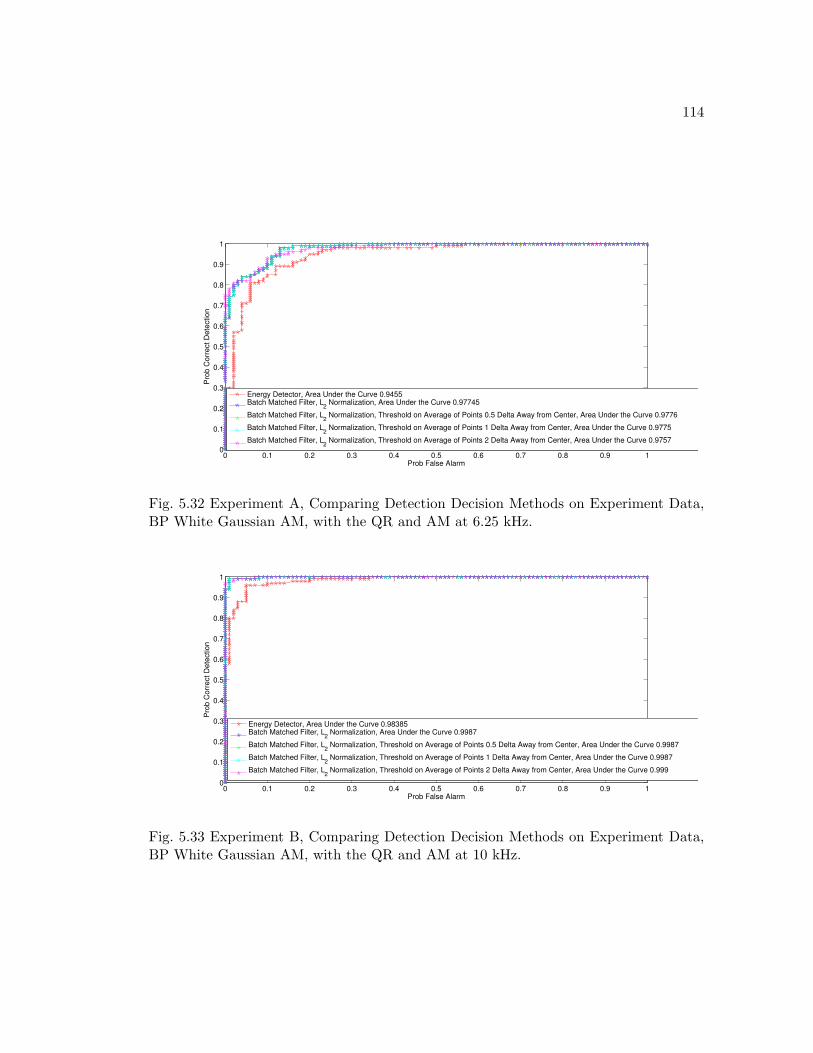
114
0 0.1 0.2 0.3 0.4 0.5 0.6 0.7 0.8 0.9 10
0.1
0.2
0.3
0.4
0.5
0.6
0.7
0.8
0.9
1
Pro
b C
orr
ect D
ete
ction
Prob False Alarm
Energy Detector, Area Under the Curve 0.9455Batch Matched Filter, L
2 Normalization, Area Under the Curve 0.97745
Batch Matched Filter, L2 Normalization, Threshold on Average of Points 0.5 Delta Away from Center, Area Under the Curve 0.9776
Batch Matched Filter, L2 Normalization, Threshold on Average of Points 1 Delta Away from Center, Area Under the Curve 0.9775
Batch Matched Filter, L2 Normalization, Threshold on Average of Points 2 Delta Away from Center, Area Under the Curve 0.9757
Fig. 5.32 Experiment A, Comparing Detection Decision Methods on Experiment Data,BP White Gaussian AM, with the QR and AM at 6.25 kHz.
0 0.1 0.2 0.3 0.4 0.5 0.6 0.7 0.8 0.9 10
0.1
0.2
0.3
0.4
0.5
0.6
0.7
0.8
0.9
1
Pro
b C
orr
ect D
ete
ction
Prob False Alarm
Energy Detector, Area Under the Curve 0.98385Batch Matched Filter, L
2 Normalization, Area Under the Curve 0.9987
Batch Matched Filter, L2 Normalization, Threshold on Average of Points 0.5 Delta Away from Center, Area Under the Curve 0.9987
Batch Matched Filter, L2 Normalization, Threshold on Average of Points 1 Delta Away from Center, Area Under the Curve 0.9987
Batch Matched Filter, L2 Normalization, Threshold on Average of Points 2 Delta Away from Center, Area Under the Curve 0.999
Fig. 5.33 Experiment B, Comparing Detection Decision Methods on Experiment Data,BP White Gaussian AM, with the QR and AM at 10 kHz.
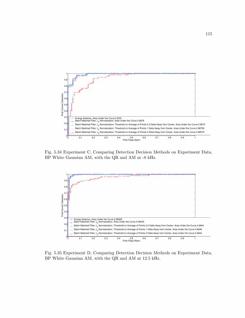
115
0 0.1 0.2 0.3 0.4 0.5 0.6 0.7 0.8 0.9 10
0.1
0.2
0.3
0.4
0.5
0.6
0.7
0.8
0.9
1
Pro
b C
orr
ect D
ete
ction
Prob False Alarm
Energy Detector, Area Under the Curve 0.9231Batch Matched Filter, L
2 Normalization, Area Under the Curve 0.9878
Batch Matched Filter, L2 Normalization, Threshold on Average of Points 0.5 Delta Away from Center, Area Under the Curve 0.9879
Batch Matched Filter, L2 Normalization, Threshold on Average of Points 1 Delta Away from Center, Area Under the Curve 0.98795
Batch Matched Filter, L2 Normalization, Threshold on Average of Points 2 Delta Away from Center, Area Under the Curve 0.98575
Fig. 5.34 Experiment C, Comparing Detection Decision Methods on Experiment Data,BP White Gaussian AM, with the QR and AM at -8 kHz.
0 0.1 0.2 0.3 0.4 0.5 0.6 0.7 0.8 0.9 10
0.1
0.2
0.3
0.4
0.5
0.6
0.7
0.8
0.9
1
Pro
b C
orr
ect D
ete
ction
Prob False Alarm
Energy Detector, Area Under the Curve 0.95655Batch Matched Filter, L
2 Normalization, Area Under the Curve 0.99435
Batch Matched Filter, L2 Normalization, Threshold on Average of Points 0.5 Delta Away from Center, Area Under the Curve 0.9944
Batch Matched Filter, L2 Normalization, Threshold on Average of Points 1 Delta Away from Center, Area Under the Curve 0.9946
Batch Matched Filter, L2 Normalization, Threshold on Average of Points 2 Delta Away from Center, Area Under the Curve 0.9944
Fig. 5.35 Experiment D, Comparing Detection Decision Methods on Experiment Data,BP White Gaussian AM, with the QR and AM at 12.5 kHz.
116
The following chapter introduces an approach that utilizes a noise estimate to better
match the filter to the noise present, instead of designing the matched filter on the
assumption that the noise present is white.
117
Chapter 6
Batch Whitened Matched Filter
The previous chapter introduced the batch matched filter and its performance was com-
pared to the generic energy detector, where it was shown to outperform it. That filter
attempts to match to the QR signal, had one been present in the received signal, though
it does not utilize any information about the noise to better improve the detection per-
formance. The selected filter out of the batch of matched filters would be the linear filter
that maximizes SNR (Equation 4.8), if it exactly matched the QR signal and the present
noise is white. Unfortunately, AM noise is not white, therefore the batch matched filter
is not optimal even if it locks to the right QR signal.
To be able to design the matched filter that maximizes SNR, not only is an exact descrip-
tion of the QR signal required but so is the second moment of the noise present. Since
AM noise is not stationary, the noise statistics change, we are unable to design a filter
matched to both the QR signal and the noise. In Section (5.3), we used a “brute force”
gridding technique to match to the QR signal present. This is combined with a method
introduced in this chapter that provides an estimate of the noise statistics and leads to
a filter that is better matched to the noise present. Before introducing the method that
will provide an estimate of the noise statistics, we need to overcome the non-stationarity
challenge of the AM noise. To do that, we will assume the following,
118
Assumption 5. Assume that throughout the length of a single echo (less than 2 ms), an
averaged AM noise signal is wide sense stationary, i.e. the first and second moments do
not vary with respect to time.
The above assumption is a reasonable one, since the length of an echo window is very
short. Based on the above assumption the received AM signal in Equation (3.22), consists
of Nm wide sense stationary, WSS, AM signals strung in time. So each ηpci is a WSS
signal with its own noise statistics. This enables us to design a string of matched filters,
where each is matched to the QR signal present and a different set of noise statistics.
The chapter starts by introducing a batch whitened matched filter with a fixed order
whitening filter. The chapter then moves on to introducing methods that adaptively
select the whitening filter order and compares their performance.
6.1 Whitened Matched Filter
In a typical QR detection applications such as landmine detection and luggage scanning
the SNR is very low due to external RF interferences [9; 31]. Therefore, if the weak
stationarity condition holds (Assumption 5) and the noise statistics are unknown, an
estimate of the noise statistics can be obtained from the received signal if the following
assumption, which is reasonable in QR detection applications, holds.
Assumption 6. Assume that phase-cycled echo, xpc, has low SNR ratio, i.e. the value
of the QR signal is very small when compared to the present noise.
If the received phase cycled signal, xpc[k], and present noise, χpc[k], are
119
xpc[k] = spc[k] + ηpc[k] + npc[k]
χpc[k] = ηpc[k] + npc[k]
we are unable to obtain the noise statistics due to the unavailability of χpc[k]. Though,
a good estimate of the received noise, χpc[k], would be the received signal, xpc[k],
χpc[k] = ηpc[k] + npc[k] = xpc[k]. (6.1)
This would lead to an error equal to the value of the QR signal, small when compared
to the value of χpc[k]
χpc[k]− χpc[k] = spc[k]
This estimate of the received noise, χpc, can be used to estimate the covariance of the
noise, Σ, and design a matched filter that uses both information about the QR signal
and the noise as follows,
h = Σ−1spc
Since Σ−1 is a real symmetric positive definite matrix, the above equation can be rewrit-
ten as
120
h = W TWspc
where W is a real nonsingular matrix. The inner product of this filter with the received
signal xpc is
y = hTxpc = (W TWspc)Txpc = (Wspc)
T (Wxpc) = (sw)Txw.
From the above equation, it becomes apparent that applying a filter, h (matched to
both the QR signal and the present noise) to the received signal, xpc is equivalent to
multiplying both the received signal, xpc, and the filter that is only matched to the
QR signal, spc, by a filtering matrix, W , before taking their inner product. Therefore,
estimating the inverse covariance matrix Σ−1 is equivalent to estimating the matrix W .
The term (sw)Txw in the above equation resembles the matched filter in the presence
of white noise, when the optimal filter is the QR signal. Therefore, we can refer to the
matrix W as the whitening matrix.
There exist several methods to estimate the whitening matrix. Some of which are based
on Prony’s all-pole modeling method, which is an approach used to model a particular
signal. Applying the inverse model to the same signal should result in white noise, hence
applying the inverse model of the received noise to the received echo, xpc, should whiten
the received noise and result in xw. Prony’s method owes its popularity to its accurate
representation of many different types of signals in many different applications. In speech
processing for example, an acoustic tube model for speech production leads to an all-pole
121
model [28]. Other reasons we chose to focus on all-pole modeling algorithms, is one their
special structure and two the small effect the inverse model (an all-zero model) has on
the QR signal, which is discussed in Section 6.1.3.
We used two all-pole modeling methods, which are based on Prony’s all-pole normal
equations, to model the signal. These two methods are introduced next and their perfor-
mance is compared later in this chapter. The first is the autocorrelation method which
is discussed in the following subsection. The second method is the covariance method,
discussed in the subsection following that. They both have their advantages and disad-
vantages as will be discussed in the following subsections, though the most important
advantage the autocorrelation method has over the covariance method is that it guaran-
tees stability of the estimated model. In our case, even if the covariance method results
in an unstable model estimate of the noise, it can still be used, since its inverse (all-zero
model) is what is used to whiten to the signal. One advantage the covariance method
has over the autocorrelation, is that it has been known to provide more accurate signal
models [28].
In our particular case, we are attempting to model an AM signal, which has a sinusoidal
component, and therefore the signal model estimate should have poles close to the unit
circle. The autocorrelation method forces these poles to fall within the unit circle, which
leads to some inaccuracy when attempting to model a sinusoidal signal. On the other
hand, since the covariance method does not place this restriction on the poles of the
model, it can lead to more accurate sinusoidal signal models.
122
6.1.1 Estimating Whitening Matrix using the Autocorrelation Method
The autocorrelation all-pole modeling method, based on Prony’s method, is introduced in
this subsection. The special structure found in the all pole Prony normal equations, lead
to fast and efficient algorithms for finding the all-pole parameters. The autocorrelation
method, also guarantees that the resulting noise model estimate is a stable one.
Assume x[n] for n = 0, 1, . . . , N −1, is the signal we would like to model the z-transform
of, using a pth order all pole model of the form
H[z] =b[0]
1 +∑p
k=1 ap[k]z−k,
then using the autocorrelation method, the all pole coefficients, ap[k], are found by
minimizing the following error
εp =∞∑n=0
|e[n]|2
where,
e[n] = x[n] +p∑
k=1
ap[k]x[n− k].
Since x[n] is only known for 0 ≤ n ≤ N − 1, the error e[n] can only be evaluated for
p ≤ n ≤ N − 1. To enable us to calculate e[n], the autocorrelation method assumes that
x[n] = 0 outside the interval [0, N − 1], which is a drawback since the signal is usually
non-zero outside the known interval. It has been shown that solving the following normal
equations for the coefficients ap[k] minimizes εp [28].
123
p∑l=1
ap[l]rx[k − l] = −rx[k]; k = 1, 2, . . . , p
rx[k] =N−1∑n=k
x[n]x∗[n− k]; k ≥ 0
These coefficients lead to a minimum error value of,
{εp}min = rx[0] +p∑
k=1
ap[k]r∗x[k]. (6.2)
Note that in our particular case, where the signals are real, the conjugates of the signals
above are equal to the signals themselves. The effect of the model order on the per-
formance of the batch whitened matched filter is discussed in Section 6.3 and different
methods of choosing the filter order are introduced in Section 6.4.
Now that an estimate model of the noise signal has been obtained, we can apply the
inverse model, 1/H[z], to the received signal, which would lead to an approximately
white signal. Therefore, this filter can be referred to as a whitening filter.
The inverse of the model is an all zero model and can be represented as follows
Hw[z] = Hinv[z] =1
H[z]=
1 +∑p
k=1 ap[k]z−k
b0,
where, b0 is a scaling factor and can be set to one without affecting the resulting whitened
signal. Applying the above whitening filter to a signal is equivalent to multiplying
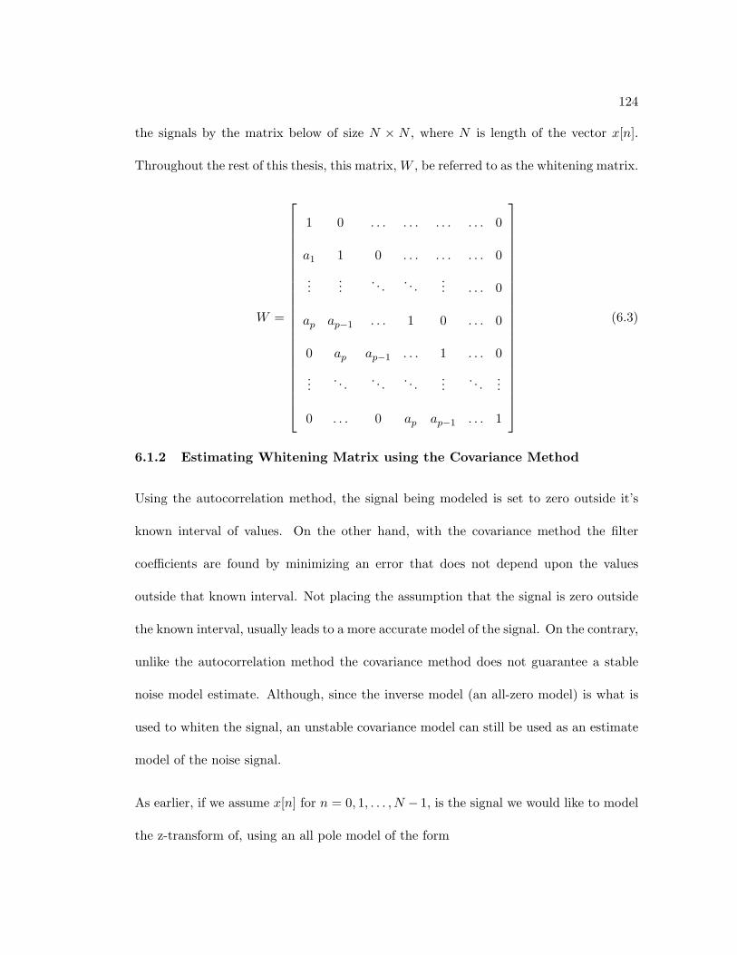
124
the signals by the matrix below of size N × N , where N is length of the vector x[n].
Throughout the rest of this thesis, this matrix, W , be referred to as the whitening matrix.
W =
1 0 . . . . . . . . . . . . 0
a1 1 0 . . . . . . . . . 0
......
. . . . . .... . . . 0
ap ap−1 . . . 1 0 . . . 0
0 ap ap−1 . . . 1 . . . 0
.... . . . . . . . .
.... . .
...
0 . . . 0 ap ap−1 . . . 1
(6.3)
6.1.2 Estimating Whitening Matrix using the Covariance Method
Using the autocorrelation method, the signal being modeled is set to zero outside it’s
known interval of values. On the other hand, with the covariance method the filter
coefficients are found by minimizing an error that does not depend upon the values
outside that known interval. Not placing the assumption that the signal is zero outside
the known interval, usually leads to a more accurate model of the signal. On the contrary,
unlike the autocorrelation method the covariance method does not guarantee a stable
noise model estimate. Although, since the inverse model (an all-zero model) is what is
used to whiten the signal, an unstable covariance model can still be used as an estimate
model of the noise signal.
As earlier, if we assume x[n] for n = 0, 1, . . . , N − 1, is the signal we would like to model
the z-transform of, using an all pole model of the form
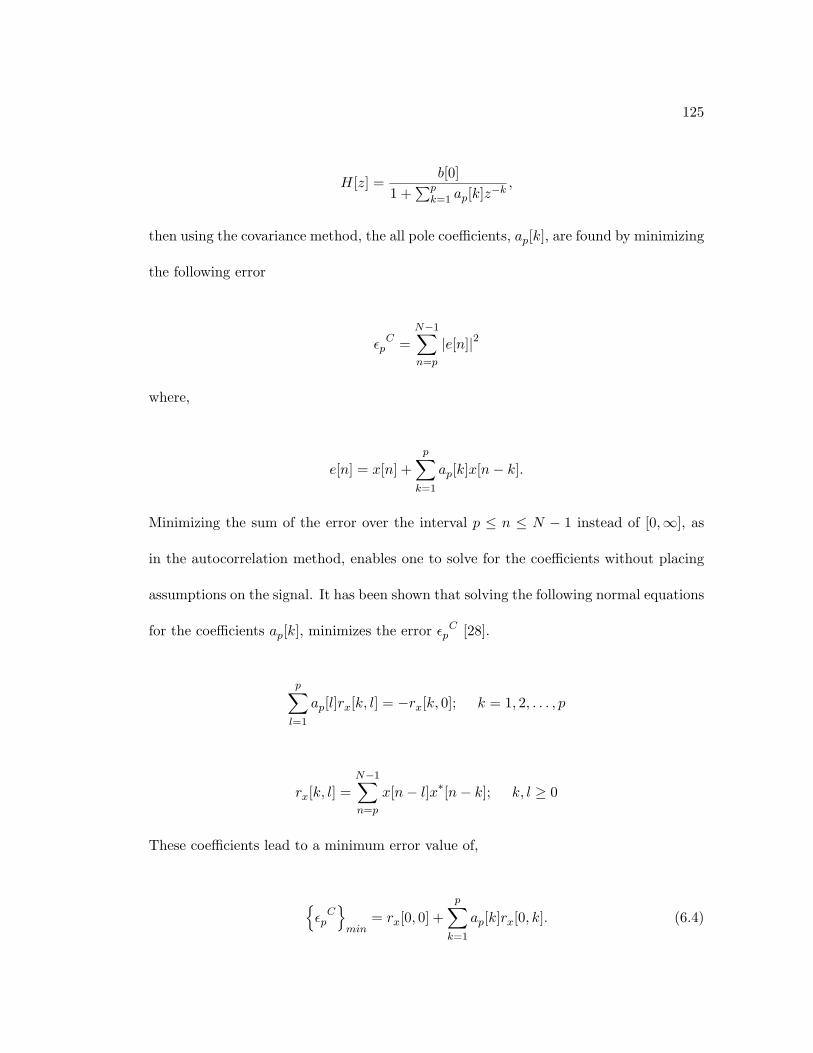
125
H[z] =b[0]
1 +∑p
k=1 ap[k]z−k,
then using the covariance method, the all pole coefficients, ap[k], are found by minimizing
the following error
εpC =
N−1∑n=p
|e[n]|2
where,
e[n] = x[n] +p∑
k=1
ap[k]x[n− k].
Minimizing the sum of the error over the interval p ≤ n ≤ N − 1 instead of [0,∞], as
in the autocorrelation method, enables one to solve for the coefficients without placing
assumptions on the signal. It has been shown that solving the following normal equations
for the coefficients ap[k], minimizes the error εpC [28].
p∑l=1
ap[l]rx[k, l] = −rx[k, 0]; k = 1, 2, . . . , p
rx[k, l] =N−1∑n=p
x[n− l]x∗[n− k]; k, l ≥ 0
These coefficients lead to a minimum error value of,
{εpC}min
= rx[0, 0] +p∑
k=1
ap[k]rx[0, k]. (6.4)
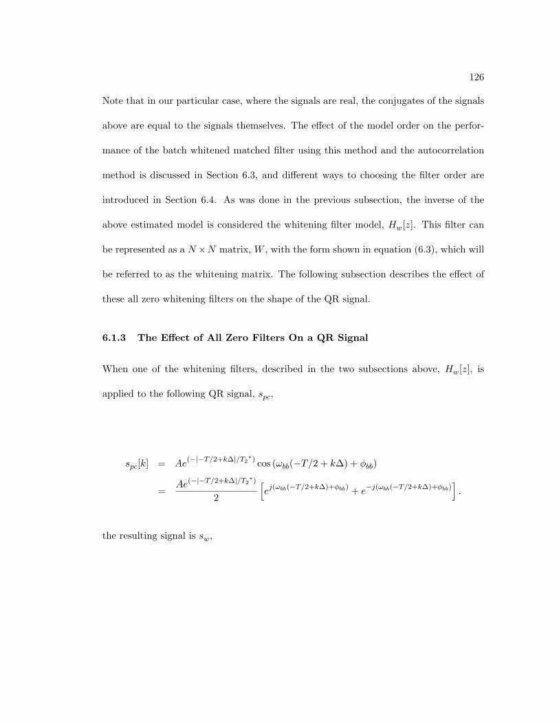
126
Note that in our particular case, where the signals are real, the conjugates of the signals
above are equal to the signals themselves. The effect of the model order on the perfor-
mance of the batch whitened matched filter using this method and the autocorrelation
method is discussed in Section 6.3, and different ways to choosing the filter order are
introduced in Section 6.4. As was done in the previous subsection, the inverse of the
above estimated model is considered the whitening filter model, Hw[z]. This filter can
be represented as a N ×N matrix, W , with the form shown in equation (6.3), which will
be referred to as the whitening matrix. The following subsection describes the effect of
these all zero whitening filters on the shape of the QR signal.
6.1.3 The Effect of All Zero Filters On a QR Signal
When one of the whitening filters, described in the two subsections above, Hw[z], is
applied to the following QR signal, spc,
spc[k] = Ae(−|−T/2+k∆|/T2∗) cos (ωbb(−T/2 + k∆) + φbb)
=Ae(−|−T/2+k∆|/T2
∗)
2
[ej(ωbb(−T/2+k∆)+φbb) + e−j(ωbb(−T/2+k∆)+φbb)
].
the resulting signal is sw,
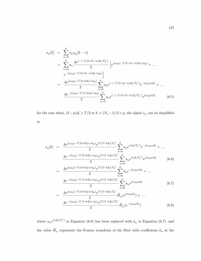
127
sw[k] =p∑
n=0
anspc[k − n]
=p∑
n=0
anAe(−|−T/2+(k−n)∆|/T2
∗)
2
[ej(ωbb(−T/2+(k−n)∆)+φbb) + . . .
e−j(ωbb(−T/2+(k−n)∆)+φbb)]
=Aej(ωbb(−T/2+k∆)+φbb)
2
p∑n=0
ane(−|−T/2+(k−n)∆|/T2
∗)e−j(ωbbn∆) + . . .
Ae−j(ωbb(−T/2+k∆)+φbb)
2
p∑n=0
ane(−|−T/2+(k−n)∆|/T2
∗)ej(ωbbn∆) (6.5)
for the case when, (k− p)∆ ≥ T/2 or k ≥ (Ns− 1)/2 + p, the signal sw can be simplified
to
sw[k] =Aej(ωbb(−T/2+k∆)+φbb)e(T/2−k∆)/T2
∗
2
p∑n=0
ane(n∆/T2
∗)e−j(ωbbn∆) + . . .
Ae−j(ωbb(−T/2+k∆)+φbb)e(T/2−k∆)/T2∗
2
p∑n=0
ane(n∆/T2
∗)ej(ωbbn∆) (6.6)
=Aej(ωbb(−T/2+k∆)+φbb)e(T/2−k∆)/T2
∗
2
p∑n=0
ane−j(ωbbn∆) + . . .
Ae−j(ωbb(−T/2+k∆)+φbb)e(T/2−k∆)/T2∗
2
p∑n=0
anej(ωbbn∆) (6.7)
=Aej(ωbb(−T/2+k∆)+φbb)e(T/2−k∆)/T2
∗
2Hw(ej(ωbb∆)) + . . .
Ae−j(ωbb(−T/2+k∆)+φbb)e(T/2−k∆)/T2∗
2Hw(e−j(ωbb∆)) (6.8)
where ane(n∆/T2
∗) in Equation (6.6) has been replaced with an in Equation (6.7), and
the value Hw represents the Fourier transform of the filter with coefficients an at the
128
frequency ωbb∆. Since, FIR filters with real coefficients have conjugate symmetry, i.e
Hw(e−j(ωbb∆)) = H∗w
(ej(ωbb∆)), as follows
Hw(e−j(ωbb∆)) = Re{H(ej(ωbb∆))} − jIm{H(ej(ωbb∆))}
= |H(ej(ωbb∆))|{−∠H(ej(ωbb∆))}
the Equation (6.8) can be rewritten as
sw[k] =A
2
∣∣∣Hw
(ej(ωbb∆)
)∣∣∣ e(T/2−k∆)/T2∗ [ej(ωbb(−T/2+k∆)+φbb+〈Hw(ej(ωbb∆))) + . . .
e−j(ωbb(−T/2+k∆)+φbb+〈Hw(ej(ωbb∆)))]
= A∣∣∣Hw
(ej(ωbb∆)
)∣∣∣ e(T/2−k∆)/T2∗
cos(ωbb(−T/2 + k∆) + φbb + 〈Hw
(ej(ωbb∆)
)). (6.9)
The above equation shows that for k ≥ (Ns − 1)/2 + p the whitening filter only affects
the magnitude and phase of the QR signal and keeps the shape and frequency of the
signal intact. Using the same procedure above it can be shown that for the case when
k ≤ (Ns − 1)/2 the whitening filter again only affects the magnitude and phase of the
signal, leaving the shape and frequency intact. Due to the similarity of the derivation
with the previous step, only a general overview of the derivation will be presented. For
k ≤ (Ns− 1)/2, the processed QR signal at the output of the QR signal, Equation (6.5),
is reduced to
129
sw[k] =Aej(ωbb(−T/2+k∆)+φbb)e(−T/2+k∆)/T2
∗
2
p∑n=0
ane(−n∆/T2
∗)e−j(ωbbn∆) + . . .
Ae−j(ωbb(−T/2+k∆)+φbb)e(−T/2+k∆)/T2∗
2
p∑n=0
ane(−n∆/T2
∗)ej(ωbbn∆)
=Aej(ωbb(−T/2+k∆)+φbb)e(−T/2+k∆)/T2
∗
2
p∑n=0
ane−j(ωbbn∆) + . . .
Ae−j(ωbb(−T/2+k∆)+φbb)e(−T/2+k∆)/T2∗
2
p∑n=0
anej(ωbbn∆)
=Aej(ωbb(−T/2+k∆)+φbb)e(−T/2+k∆)/T2
∗
2Hw(ej(ωbb∆)) + . . .
Ae−j(ωbb(−T/2+k∆)+φbb)e(−T/2+k∆)/T2∗
2Hw(e−j(ωbb∆))
=A
2
∣∣∣Hw
(ej(ωbb∆)
)∣∣∣ e(−T/2+k∆)/T2∗ [ej(ωbb(−T/2+k∆)+φbb+〈Hw(ej(ωbb∆))) + . . .
e−j(ωbb(−T/2+k∆)+φbb+〈Hw(ej(ωbb∆)))]
= A∣∣∣Hw
(ej(ωbb∆)
)∣∣∣ e(−T/2+k∆)/T2∗
cos(ωbb(−T/2 + k∆) + φbb + 〈Hw
(ej(ωbb∆)
)). (6.10)
Equations (6.10), for k ≤ (Ns − 1)/2, and (6.9), for k ≥ (Ns − 1)/2 + p, show that
the shape and frequency of the whitened QR signal remain unchanged and only the
magnitude and phase are affected. For the p−1 values, (Ns−1)/2 < k < (Ns−1)/2+p,
the shape of the QR signal may be altered depending on the filter, and the result is
described using Equation (6.5). To demonstrate how small the effect of the FIR filter is
on the general shape of the QR signal, a simulated QR signal of frequency 12.5 is passed
through a random 6th order FIR filter and the output is compared to the input in Figure
6.1. The plot shows that the effect of the FIR filter is small.
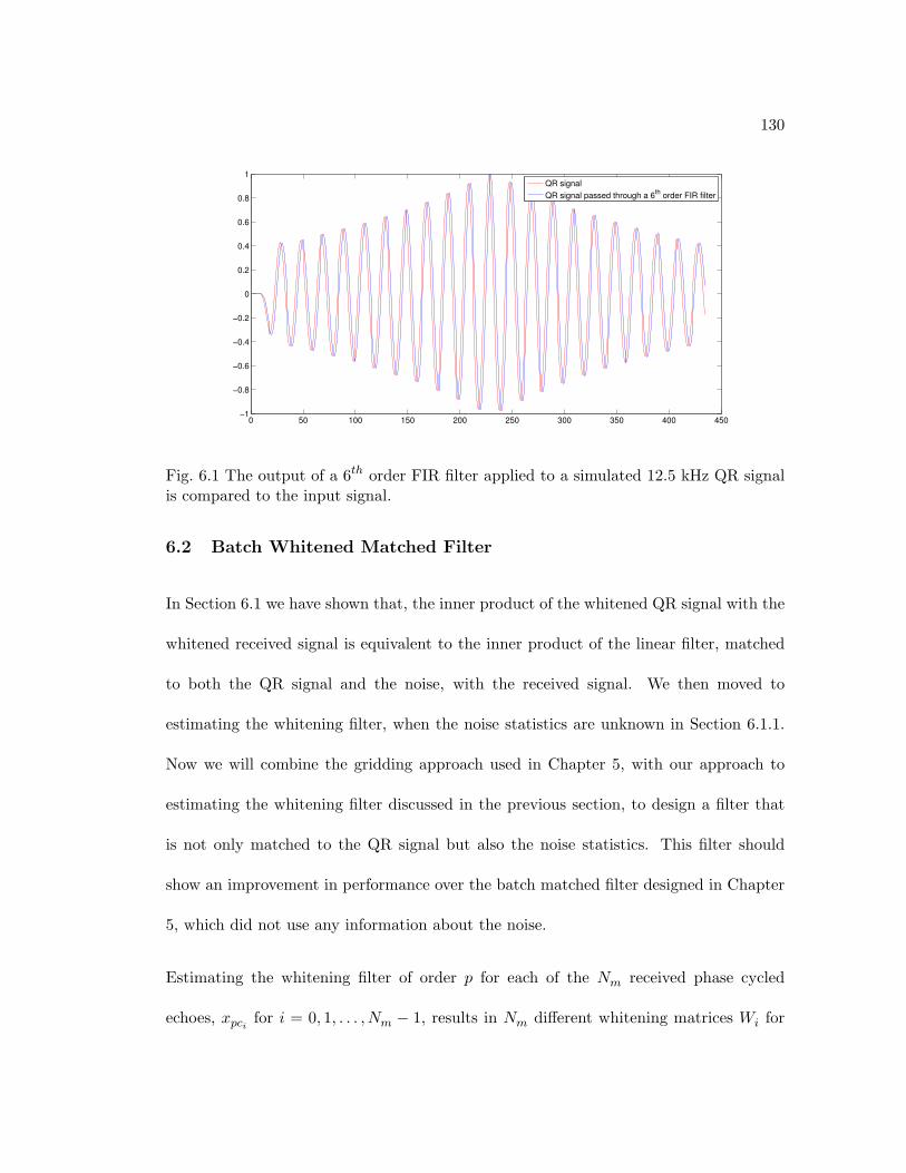
130
0 50 100 150 200 250 300 350 400 450−1
−0.8
−0.6
−0.4
−0.2
0
0.2
0.4
0.6
0.8
1
QR signal
QR signal passed through a 6th
order FIR filter
Fig. 6.1 The output of a 6th order FIR filter applied to a simulated 12.5 kHz QR signalis compared to the input signal.
6.2 Batch Whitened Matched Filter
In Section 6.1 we have shown that, the inner product of the whitened QR signal with the
whitened received signal is equivalent to the inner product of the linear filter, matched
to both the QR signal and the noise, with the received signal. We then moved to
estimating the whitening filter, when the noise statistics are unknown in Section 6.1.1.
Now we will combine the gridding approach used in Chapter 5, with our approach to
estimating the whitening filter discussed in the previous section, to design a filter that
is not only matched to the QR signal but also the noise statistics. This filter should
show an improvement in performance over the batch matched filter designed in Chapter
5, which did not use any information about the noise.
Estimating the whitening filter of order p for each of the Nm received phase cycled
echoes, xpci for i = 0, 1, . . . , Nm − 1, results in Nm different whitening matrices Wi for
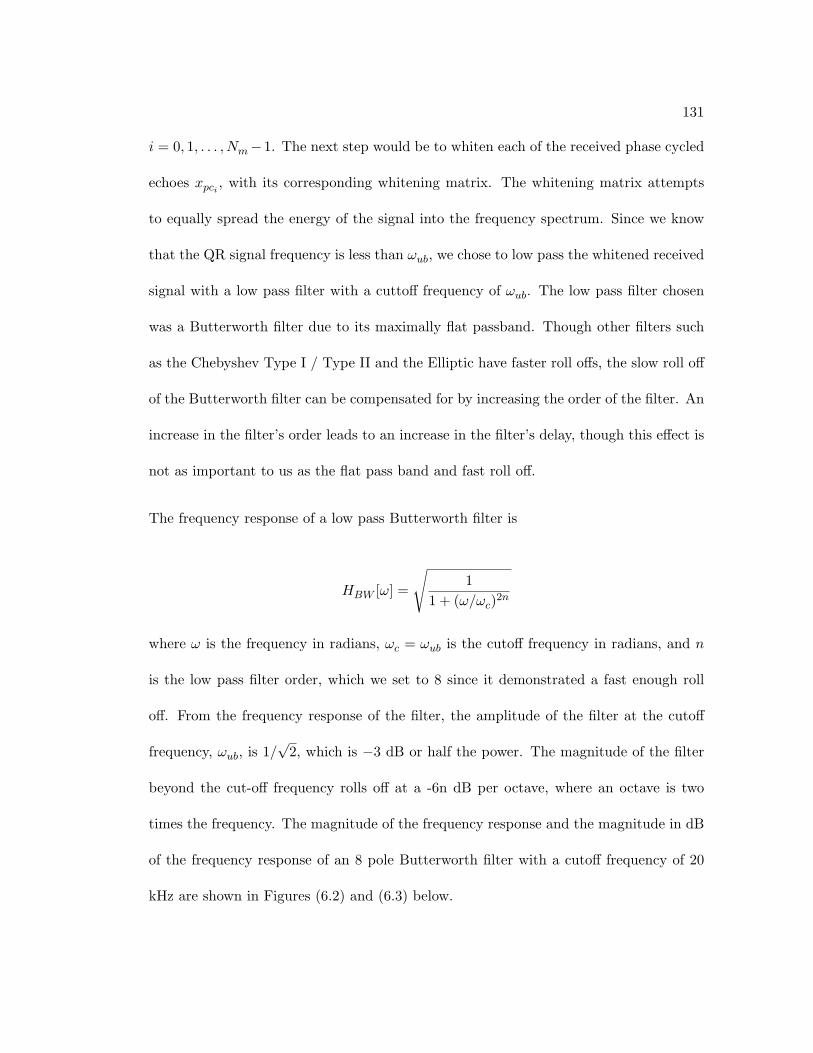
131
i = 0, 1, . . . , Nm−1. The next step would be to whiten each of the received phase cycled
echoes xpci , with its corresponding whitening matrix. The whitening matrix attempts
to equally spread the energy of the signal into the frequency spectrum. Since we know
that the QR signal frequency is less than ωub, we chose to low pass the whitened received
signal with a low pass filter with a cuttoff frequency of ωub. The low pass filter chosen
was a Butterworth filter due to its maximally flat passband. Though other filters such
as the Chebyshev Type I / Type II and the Elliptic have faster roll offs, the slow roll off
of the Butterworth filter can be compensated for by increasing the order of the filter. An
increase in the filter’s order leads to an increase in the filter’s delay, though this effect is
not as important to us as the flat pass band and fast roll off.
The frequency response of a low pass Butterworth filter is
HBW [ω] =
√1
1 + (ω/ωc)2n
where ω is the frequency in radians, ωc = ωub is the cutoff frequency in radians, and n
is the low pass filter order, which we set to 8 since it demonstrated a fast enough roll
off. From the frequency response of the filter, the amplitude of the filter at the cutoff
frequency, ωub, is 1/√
2, which is −3 dB or half the power. The magnitude of the filter
beyond the cut-off frequency rolls off at a -6n dB per octave, where an octave is two
times the frequency. The magnitude of the frequency response and the magnitude in dB
of the frequency response of an 8 pole Butterworth filter with a cutoff frequency of 20
kHz are shown in Figures (6.2) and (6.3) below.
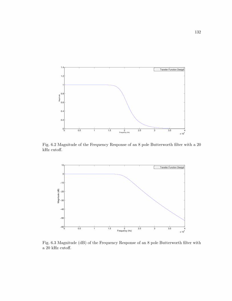
132
0 0.5 1 1.5 2 2.5 3 3.5 4
x 104
0
0.2
0.4
0.6
0.8
1
1.2
1.4
Frequency (Hz)
Magnitude
Transfer Function Design
Fig. 6.2 Magnitude of the Frequency Response of an 8 pole Butterworth filter with a 20kHz cutoff.
0 0.5 1 1.5 2 2.5 3 3.5 4
x 104
−60
−50
−40
−30
−20
−10
0
10
Frequency (Hz)
Magnitude (
dB
)
Transfer Function Design
Fig. 6.3 Magnitude (dB) of the Frequency Response of an 8 pole Butterworth filter witha 20 kHz cutoff.
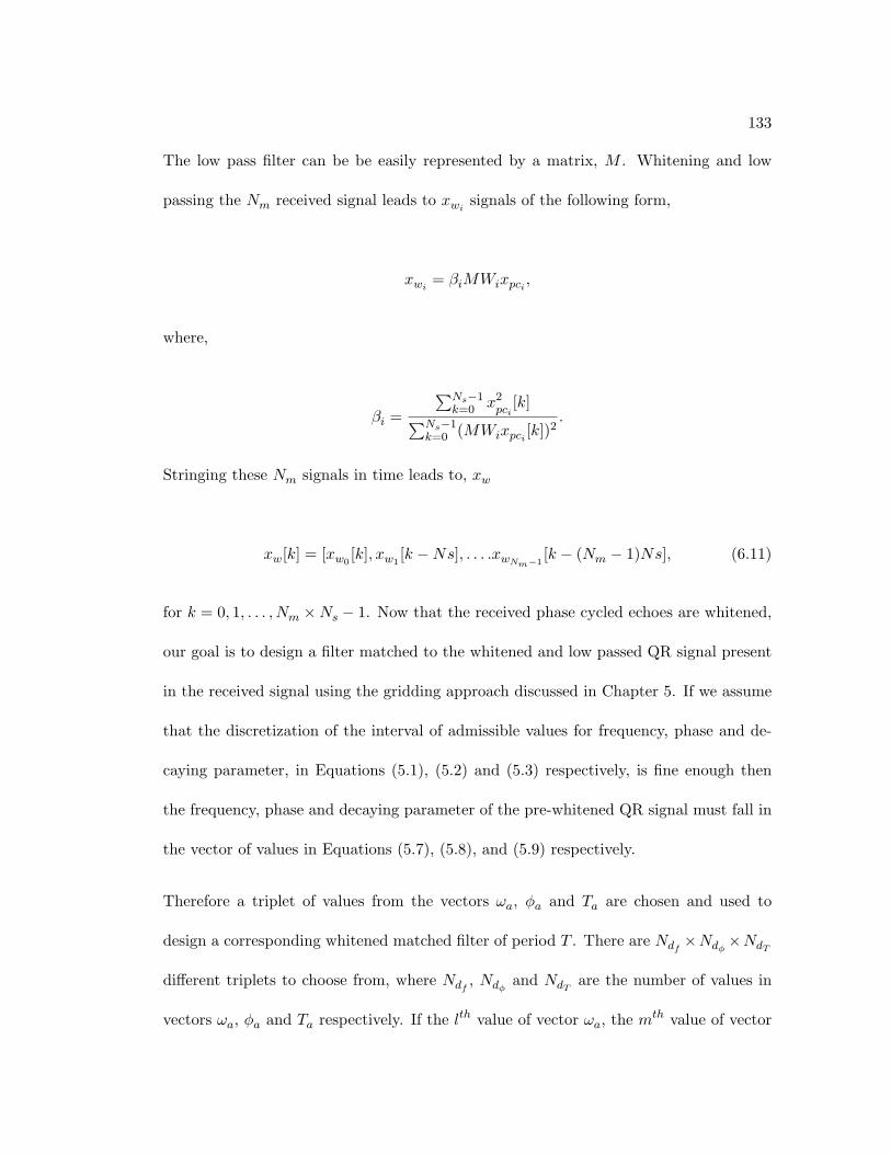
133
The low pass filter can be be easily represented by a matrix, M . Whitening and low
passing the Nm received signal leads to xwi signals of the following form,
xwi = βiMWixpci ,
where,
βi =
∑Ns−1k=0
x2pci
[k]∑Ns−1k=0 (MWixpci [k])2
.
Stringing these Nm signals in time leads to, xw
xw[k] = [xw0[k], xw1
[k −Ns], . . . .xwNm−1[k − (Nm − 1)Ns], (6.11)
for k = 0, 1, . . . , Nm ×Ns − 1. Now that the received phase cycled echoes are whitened,
our goal is to design a filter matched to the whitened and low passed QR signal present
in the received signal using the gridding approach discussed in Chapter 5. If we assume
that the discretization of the interval of admissible values for frequency, phase and de-
caying parameter, in Equations (5.1), (5.2) and (5.3) respectively, is fine enough then
the frequency, phase and decaying parameter of the pre-whitened QR signal must fall in
the vector of values in Equations (5.7), (5.8), and (5.9) respectively.
Therefore a triplet of values from the vectors ωa, φa and Ta are chosen and used to
design a corresponding whitened matched filter of period T . There are Ndf ×Ndφ ×NdT
different triplets to choose from, where Ndf , Ndφ and NdT are the number of values in
vectors ωa, φa and Ta respectively. If the lth value of vector ωa, the mth value of vector
134
φa and the nth value of vector Ta are the chosen values then the corresponding estimate
of the whitened low passed matched filter for phase cycled echo, i, is
swi(l,m, n)[k] =1
αwi(l,m, n)MWie
(−|−T/2+k∆|/Ta(n))cos(ωa(l)(−T/2 + k∆) + φa(m))
for k = 0, 1, . . . , Ns − 1. The value T is the length of the data acquisition window, Ns is
the number of discrete samples, ∆ = T/(Ns − 1) and the constant αwi(l,m, n) is
αwi(l,m, n) =
√√√√Ns−1∑k=0
[MWie(−|−T/2+k∆|/Ta(n))cos(ωa(l)(−T/2 + k∆) + φa(m))]2.
Therefore, the estimated whitened low passed matched filter for the above QR signal
parameter values chosen, comprises of the Nm whitened low passed matched filters,
swi(l,m, n), strung in time,
h[k] = [sw0(l,m, n)[k], sw1
(l,m, n)[k −Ns], . . . , swNm−1(l,m, n)[k − (Nm− 1)Ns],
for k = 0, 1, . . . , Nm×Ns−1. After sending our received whitened signal through the filter
with the above impulse response, the value of the Nm ×Nsth sample, which is equivalent
to the inner product of the received whitened signal and the estimated whitened matched
filter, is recorded. This process is repeated for a different combination of values for the
135
frequency ωbb, φbb and decaying parameter T2∗. Repeating this experiment Ndf ×Ndφ ×
NdT times leads to a vector Θ of values of length Ndf ×Ndφ ×NdT .
Θ = [θ1, . . . , θNdf×Ndφ×NdT] (6.12)
Finally the maximum value of the vector Θ is compared to a threshold value θthreshold and
the filter corresponding to this maximum is the chosen filter out of the whitened batch of
filters. If the maximum value is greater than the threshold then we would conclude that
a QR signal exists within the corrupted signal, otherwise we would conclude that the
received signal is just noise. The process of choosing the filter is equivalent to selecting
the filter, hn[k], that maximizes yn, the inner product of the filter with the whitened
received signal xw[k] in Equation (6.11), over the set of possible filters as follows
y = maxn
(yn) = maxn
(hn[k]Txw[k]
)= max
n
(|hn[k]||xw[k]| cos γ
)
where γ is the angle between the received signal, xw[k], and the filter hn[k]. If the
chosen filter out of the batch is equal to the whitened QR signal present, sw[k], then the
resulting signal to noise ratio defined in Equation (4.8) is reduced to
ρ(sw; sw, I) =(sw[k]T sw[k])2
sw[k]T Isw[k]= (sw[k]T sw[k]) = (s[k]TΣ−1s[k])
where I is the identity matrix and corresponds the covariance of the noise after whitening,
assuming the whitening filter is exact. The matrix, Σ, on the other hand is the covariance
of the noise pre-whitening. The above signal to noise ratio is the same as the signal
136
noise ratio resulting from the optimal matched filter, shown in Equation (4.11). This
is expected since we are assuming that the estimate of the whitening filter is exact and
the chosen whitened filter out of the whitened batch of filters is the whitened QR signal
present, which would lead to an optimal matched filter.
6.3 Batch Whitened Matched Filter versus Energy Detector, Unknown
QR signal
Simulation data was first used, to test the performance of several batch whitened matched
filters for a range of whitening filter orders, where the whitening filter was designed
using either the autocorrelation or the covariance method. The performance of these
filters was then compared it to the performance of the batch matched filter, described in
Chapter 5, and the energy detector. These filters were the compared using experimental
data. For both the autocorrelation and covariance methods, the problem of choosing the
order of the all zero whitening filter has not been addressed and the order was varied
between 3 and 7, to evaluate the performance of the batch whitened matched filter
for different whitening filter orders. Section 6.4 introduces two different methods for
choosing the whitening filter order and compares their performance. The order of the
low pass butterworth filter on the other hand, was fixed to 8 with a cutoff frequency of
20 kHz.
6.3.1 Simulation Data
Six sets of simulation data, the same ones used to compare the batch matched filter to
the energy detector, where the QR and the AM baseband frequencies were equal. The
137
first set had a frequency of 2.5 kHz, and the frequency was increased by 2.5 kHz for each
following set, leading to a frequency of 15 kHz for the sixth data set. The simulation
data setup and batch matched filter gridding parameters are provided in section 5.3.1,
therefore they will not be repeated here.
The batch whitened matched filters, for both the autocorrelation and the covariance
whitening methods with the different whitening filter orders, used the following values
to grid, ωlb = 0, ωub = 40000π, ω∆ = 200π, φ∆ = .1, T ∗2 lb
= 800e− 6, T ∗2 ub
= 1000e− 6
and T ∗2 ∆
= 100e − 6. The above values lead to Ndf = 201, Ndφ = 63 and NdT = 3 in
each of the three dimensions, which corresponds to Ndf × Ndφ × NdT = 34, 989 filters
in the batch. The number of filters in the batch was reduced for the batch whitened
matched filter when compared to the batch matched filter due to the increase in each
filter’s computation time. The increase in computation time is a result of having to
whiten each filter in the batch with Nm different whitening filters, Wi, for i = 1, . . . , Nm.
The performance of the batch whitened matched filter might be slightly improved had
the gridding been finer, i.e. a larger batch of filters are used, though this leads to an
increase in computation time. The effect of finer gridding on performance was discussed
in Section 6.3.2 and therefore will not be discussed here.
ROC plots were used to compare the performance of the batch whitened matched filter
to the batch matched filter and the energy detector. Figures (6.4-6.15) compare the
performance of the different detectors for the different frequencies. Each figure compares
the energy detector and the batch matched filter to the batch whitened matched filter,
using either the autocorrelation or the covariance method, as the whitening filter order
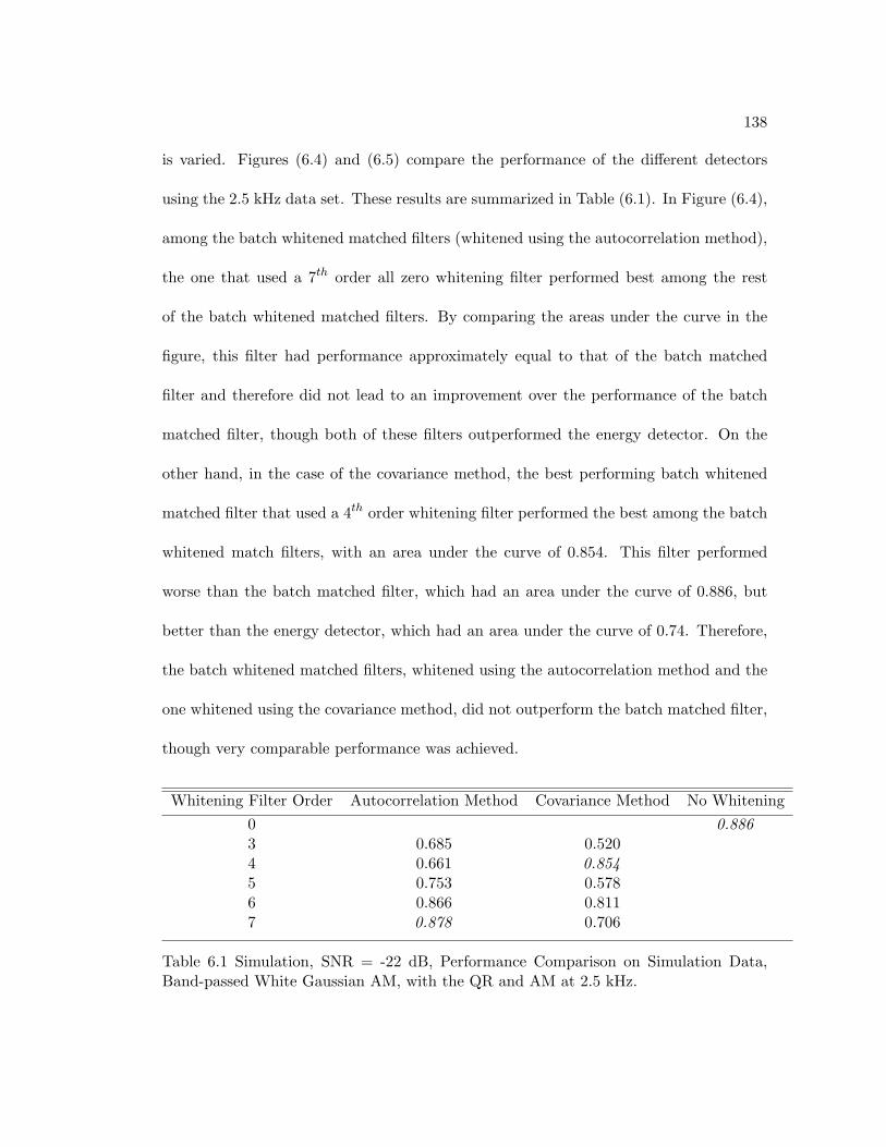
138
is varied. Figures (6.4) and (6.5) compare the performance of the different detectors
using the 2.5 kHz data set. These results are summarized in Table (6.1). In Figure (6.4),
among the batch whitened matched filters (whitened using the autocorrelation method),
the one that used a 7th order all zero whitening filter performed best among the rest
of the batch whitened matched filters. By comparing the areas under the curve in the
figure, this filter had performance approximately equal to that of the batch matched
filter and therefore did not lead to an improvement over the performance of the batch
matched filter, though both of these filters outperformed the energy detector. On the
other hand, in the case of the covariance method, the best performing batch whitened
matched filter that used a 4th order whitening filter performed the best among the batch
whitened match filters, with an area under the curve of 0.854. This filter performed
worse than the batch matched filter, which had an area under the curve of 0.886, but
better than the energy detector, which had an area under the curve of 0.74. Therefore,
the batch whitened matched filters, whitened using the autocorrelation method and the
one whitened using the covariance method, did not outperform the batch matched filter,
though very comparable performance was achieved.
Whitening Filter Order Autocorrelation Method Covariance Method No Whitening0 0.8863 0.685 0.5204 0.661 0.8545 0.753 0.5786 0.866 0.8117 0.878 0.706
Table 6.1 Simulation, SNR = -22 dB, Performance Comparison on Simulation Data,Band-passed White Gaussian AM, with the QR and AM at 2.5 kHz.
139
Figure (6.6) & (6.7) used the 5 kHz data set to compare the performance of the batch
whitened matched filters for different whitening filter orders, when estimated using the
autocorrelation method and the covariance method respectively. These results are sum-
marized in Table (6.2). Among the batch whitened matched filters, whitened with the
autocorrelation method, the best performance was achieved by the batch that used a 6th
order whitening filter. The performance of this filter, with an area under the curve of
0.894, was lower than the performance of the batch matched filter, with an area under
the curve of 0.92. Though, both these filters outperformed the energy detector, which
had an area under the curve of 0.8. In Figure (6.7), the same data set was used to
compare the performance of the batch whitened match filters for different whitening
filter orders, when estimated using the covariance method. The best filter among the
different batch whitened matched filters was achieved with a 7th order whitening filter
estimated using the covariance method, with an area under the curve of 0.97. This area
significantly outperformed both the batch matched filter and the energy detector, which
achieved areas under the curve of 0.92 and 0.8 respectively. For this particular data set,
the batch whitened matched filter, whitened using the covariance method, was able to
outperform the batch matched filter, but the batch whitened matched filter, whitened
using the autocorrelation method, did not.
The 7.5 kHz data set was used to compare the batch whitened matched filters for dif-
ferent whitening filter orders, when estimated using the autocorrelation method and the
covariance method in Figures (6.8) and (6.9) respectively. These results are summa-
rized in Table (6.3). The best performing detector among the batch whitened matched
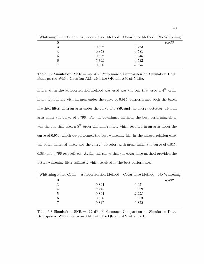
140
Whitening Filter Order Autocorrelation Method Covariance Method No Whitening0 0.9203 0.822 0.7734 0.858 0.5815 0.862 0.9456 0.894 0.5327 0.856 0.970
Table 6.2 Simulation, SNR = -22 dB, Performance Comparison on Simulation Data,Band-passed White Gaussian AM, with the QR and AM at 5 kHz.
filters, when the autocorrelation method was used was the one that used a 4th order
filter. This filter, with an area under the curve of 0.915, outperformed both the batch
matched filter, with an area under the curve of 0.889, and the energy detector, with an
area under the curve of 0.796. For the covariance method, the best performing filter
was the one that used a 5th order whitening filter, which resulted in an area under the
curve of 0.954, which outperformed the best whitening filer in the autocorrelation case,
the batch matched filter, and the energy detector, with areas under the curve of 0.915,
0.889 and 0.796 respectively. Again, this shows that the covariance method provided the
better whitening filter estimate, which resulted in the best performance.
Whitening Filter Order Autocorrelation Method Covariance Method No Whitening0 0.8893 0.894 0.9514 0.915 0.5795 0.894 0.9546 0.868 0.5537 0.847 0.852
Table 6.3 Simulation, SNR = -22 dB, Performance Comparison on Simulation Data,Band-passed White Gaussian AM, with the QR and AM at 7.5 kHz.
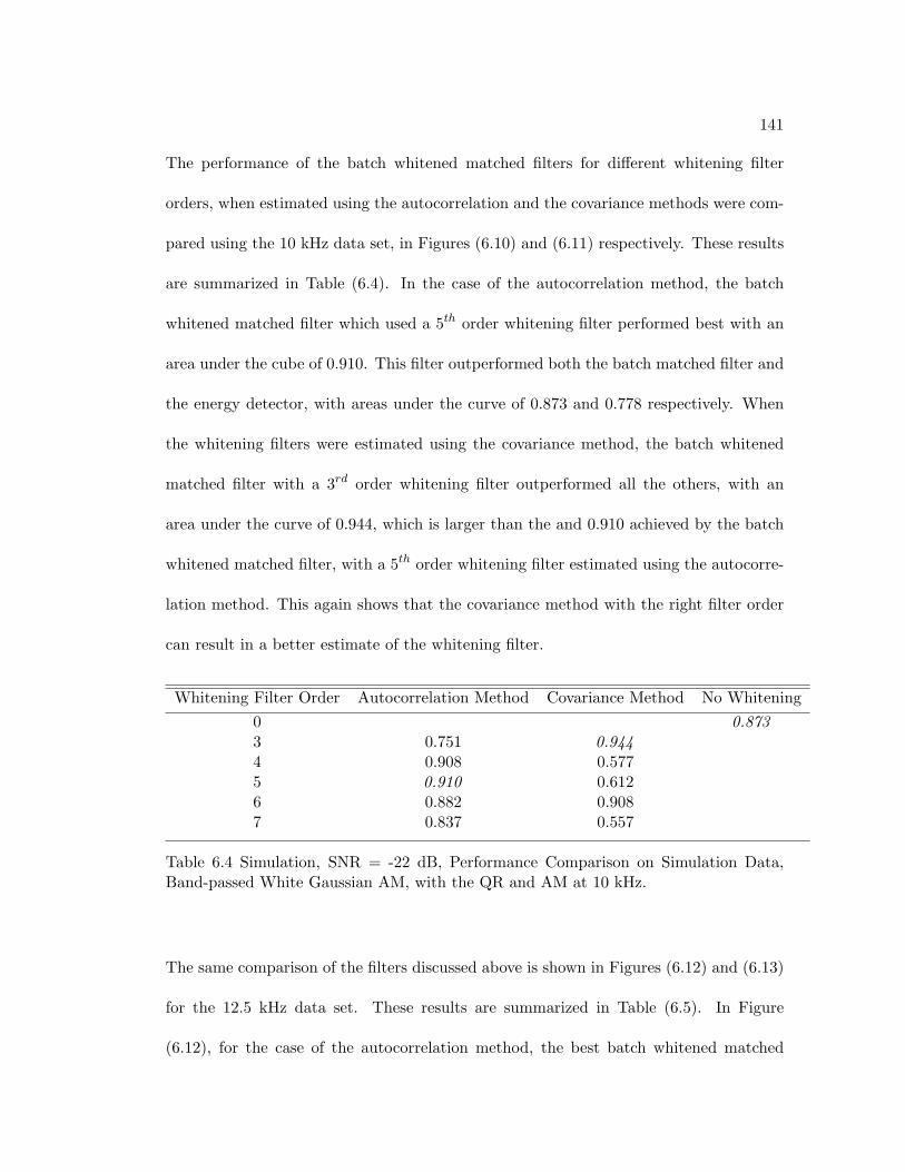
141
The performance of the batch whitened matched filters for different whitening filter
orders, when estimated using the autocorrelation and the covariance methods were com-
pared using the 10 kHz data set, in Figures (6.10) and (6.11) respectively. These results
are summarized in Table (6.4). In the case of the autocorrelation method, the batch
whitened matched filter which used a 5th order whitening filter performed best with an
area under the cube of 0.910. This filter outperformed both the batch matched filter and
the energy detector, with areas under the curve of 0.873 and 0.778 respectively. When
the whitening filters were estimated using the covariance method, the batch whitened
matched filter with a 3rd order whitening filter outperformed all the others, with an
area under the curve of 0.944, which is larger than the and 0.910 achieved by the batch
whitened matched filter, with a 5th order whitening filter estimated using the autocorre-
lation method. This again shows that the covariance method with the right filter order
can result in a better estimate of the whitening filter.
Whitening Filter Order Autocorrelation Method Covariance Method No Whitening0 0.8733 0.751 0.9444 0.908 0.5775 0.910 0.6126 0.882 0.9087 0.837 0.557
Table 6.4 Simulation, SNR = -22 dB, Performance Comparison on Simulation Data,Band-passed White Gaussian AM, with the QR and AM at 10 kHz.
The same comparison of the filters discussed above is shown in Figures (6.12) and (6.13)
for the 12.5 kHz data set. These results are summarized in Table (6.5). In Figure
(6.12), for the case of the autocorrelation method, the best batch whitened matched
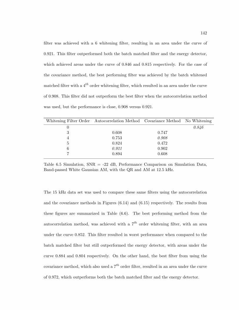
142
filter was achieved with a 6 whitening filter, resulting in an area under the curve of
0.921. This filter outperformed both the batch matched filter and the energy detector,
which achieved areas under the curve of 0.846 and 0.815 respectively. For the case of
the covariance method, the best performing filter was achieved by the batch whitened
matched filter with a 4th order whitening filter, which resulted in an area under the curve
of 0.908. This filter did not outperform the best filter when the autocorrelation method
was used, but the performance is close, 0.908 versus 0.921.
Whitening Filter Order Autocorrelation Method Covariance Method No Whitening0 0.8463 0.608 0.7474 0.753 0.9085 0.824 0.4726 0.921 0.9027 0.894 0.608
Table 6.5 Simulation, SNR = -22 dB, Performance Comparison on Simulation Data,Band-passed White Gaussian AM, with the QR and AM at 12.5 kHz.
The 15 kHz data set was used to compare these same filters using the autocorrelation
and the covariance methods in Figures (6.14) and (6.15) respectively. The results from
these figures are summarized in Table (6.6). The best performing method from the
autocorrelation method, was achieved with a 7th order whitening filter, with an area
under the curve 0.852. This filter resulted in worst performance when compared to the
batch matched filter but still outperformed the energy detector, with areas under the
curve 0.884 and 0.804 respectively. On the other hand, the best filter from using the
covariance method, which also used a 7th order filter, resulted in an area under the curve
of 0.972, which outperforms both the batch matched filter and the energy detector.
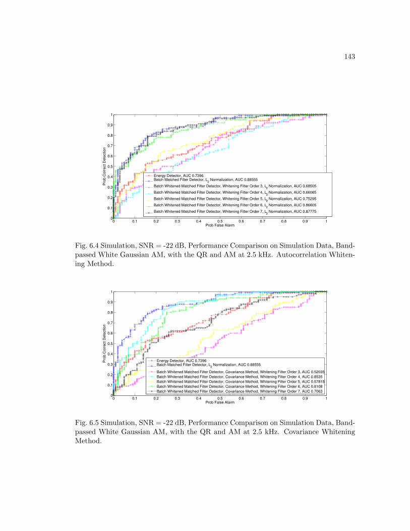
143
0 0.1 0.2 0.3 0.4 0.5 0.6 0.7 0.8 0.9 10
0.1
0.2
0.3
0.4
0.5
0.6
0.7
0.8
0.9
1
Pro
b C
orr
ect D
ete
ction
Prob False Alarm
Energy Detector, AUC 0.7396Batch Matched Filter Detector, L
2 Normalization, AUC 0.88555
Batch Whitened Matched Filter Detector, Whitening Filter Order 3, L2 Normalization, AUC 0.68505
Batch Whitened Matched Filter Detector, Whitening Filter Order 4, L2 Normalization, AUC 0.66065
Batch Whitened Matched Filter Detector, Whitening Filter Order 5, L2 Normalization, AUC 0.75295
Batch Whitened Matched Filter Detector, Whitening Filter Order 6, L2 Normalization, AUC 0.86605
Batch Whitened Matched Filter Detector, Whitening Filter Order 7, L2 Normalization, AUC 0.87775
Fig. 6.4 Simulation, SNR = -22 dB, Performance Comparison on Simulation Data, Band-passed White Gaussian AM, with the QR and AM at 2.5 kHz. Autocorrelation Whiten-ing Method.
0 0.1 0.2 0.3 0.4 0.5 0.6 0.7 0.8 0.9 10
0.1
0.2
0.3
0.4
0.5
0.6
0.7
0.8
0.9
1
Pro
b C
orr
ect D
ete
ction
Prob False Alarm
Energy Detector, AUC 0.7396Batch Matched Filter Detector, L
2 Normalization, AUC 0.88555
Batch Whitened Matched Filter Detector, Covariance Method, Whitening Filter Order 3, AUC 0.52035
Batch Whitened Matched Filter Detector, Covariance Method, Whitening Filter Order 4, AUC 0.8535
Batch Whitened Matched Filter Detector, Covariance Method, Whitening Filter Order 5, AUC 0.57815
Batch Whitened Matched Filter Detector, Covariance Method, Whitening Filter Order 6, AUC 0.8108
Batch Whitened Matched Filter Detector, Covariance Method, Whitening Filter Order 7, AUC 0.7063
Fig. 6.5 Simulation, SNR = -22 dB, Performance Comparison on Simulation Data, Band-passed White Gaussian AM, with the QR and AM at 2.5 kHz. Covariance WhiteningMethod.
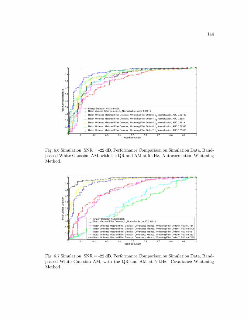
144
0 0.1 0.2 0.3 0.4 0.5 0.6 0.7 0.8 0.9 10
0.1
0.2
0.3
0.4
0.5
0.6
0.7
0.8
0.9
1
Pro
b C
orr
ect D
ete
ction
Prob False Alarm
Energy Detector, AUC 0.80095Batch Matched Filter Detector, L
2 Normalization, AUC 0.92015
Batch Whitened Matched Filter Detector, Whitening Filter Order 3, L2 Normalization, AUC 0.82195
Batch Whitened Matched Filter Detector, Whitening Filter Order 4, L2 Normalization, AUC 0.8581
Batch Whitened Matched Filter Detector, Whitening Filter Order 5, L2 Normalization, AUC 0.8619
Batch Whitened Matched Filter Detector, Whitening Filter Order 6, L2 Normalization, AUC 0.89385
Batch Whitened Matched Filter Detector, Whitening Filter Order 7, L2 Normalization, AUC 0.85555
Fig. 6.6 Simulation, SNR = -22 dB, Performance Comparison on Simulation Data, Band-passed White Gaussian AM, with the QR and AM at 5 kHz. Autocorrelation WhiteningMethod.
0 0.1 0.2 0.3 0.4 0.5 0.6 0.7 0.8 0.9 10
0.1
0.2
0.3
0.4
0.5
0.6
0.7
0.8
0.9
1
Pro
b C
orr
ect D
ete
ction
Prob False Alarm
Energy Detector, AUC 0.80095Batch Matched Filter Detector, L
2 Normalization, AUC 0.92015
Batch Whitened Matched Filter Detector, Covariance Method, Whitening Filter Order 3, AUC 0.7734
Batch Whitened Matched Filter Detector, Covariance Method, Whitening Filter Order 4, AUC 0.58105
Batch Whitened Matched Filter Detector, Covariance Method, Whitening Filter Order 5, AUC 0.945
Batch Whitened Matched Filter Detector, Covariance Method, Whitening Filter Order 6, AUC 0.5322
Batch Whitened Matched Filter Detector, Covariance Method, Whitening Filter Order 7, AUC 0.97035
Fig. 6.7 Simulation, SNR = -22 dB, Performance Comparison on Simulation Data, Band-passed White Gaussian AM, with the QR and AM at 5 kHz. Covariance WhiteningMethod.
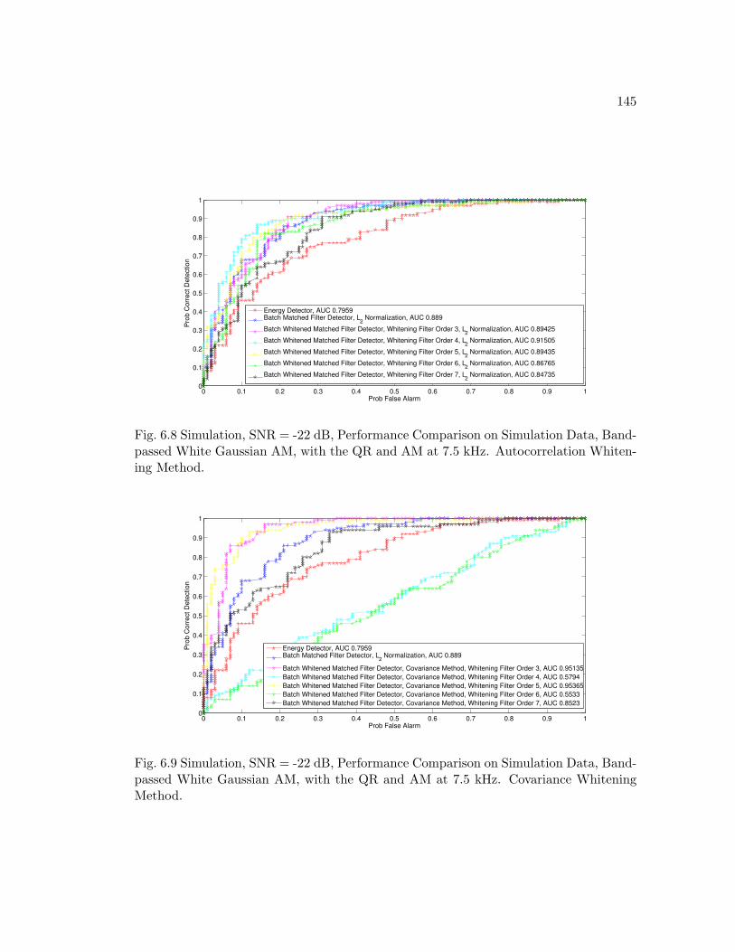
145
0 0.1 0.2 0.3 0.4 0.5 0.6 0.7 0.8 0.9 10
0.1
0.2
0.3
0.4
0.5
0.6
0.7
0.8
0.9
1
Pro
b C
orr
ect D
ete
ction
Prob False Alarm
Energy Detector, AUC 0.7959Batch Matched Filter Detector, L
2 Normalization, AUC 0.889
Batch Whitened Matched Filter Detector, Whitening Filter Order 3, L2 Normalization, AUC 0.89425
Batch Whitened Matched Filter Detector, Whitening Filter Order 4, L2 Normalization, AUC 0.91505
Batch Whitened Matched Filter Detector, Whitening Filter Order 5, L2 Normalization, AUC 0.89435
Batch Whitened Matched Filter Detector, Whitening Filter Order 6, L2 Normalization, AUC 0.86765
Batch Whitened Matched Filter Detector, Whitening Filter Order 7, L2 Normalization, AUC 0.84735
Fig. 6.8 Simulation, SNR = -22 dB, Performance Comparison on Simulation Data, Band-passed White Gaussian AM, with the QR and AM at 7.5 kHz. Autocorrelation Whiten-ing Method.
0 0.1 0.2 0.3 0.4 0.5 0.6 0.7 0.8 0.9 10
0.1
0.2
0.3
0.4
0.5
0.6
0.7
0.8
0.9
1
Pro
b C
orr
ect D
ete
ction
Prob False Alarm
Energy Detector, AUC 0.7959Batch Matched Filter Detector, L
2 Normalization, AUC 0.889
Batch Whitened Matched Filter Detector, Covariance Method, Whitening Filter Order 3, AUC 0.95135
Batch Whitened Matched Filter Detector, Covariance Method, Whitening Filter Order 4, AUC 0.5794
Batch Whitened Matched Filter Detector, Covariance Method, Whitening Filter Order 5, AUC 0.95365
Batch Whitened Matched Filter Detector, Covariance Method, Whitening Filter Order 6, AUC 0.5533
Batch Whitened Matched Filter Detector, Covariance Method, Whitening Filter Order 7, AUC 0.8523
Fig. 6.9 Simulation, SNR = -22 dB, Performance Comparison on Simulation Data, Band-passed White Gaussian AM, with the QR and AM at 7.5 kHz. Covariance WhiteningMethod.
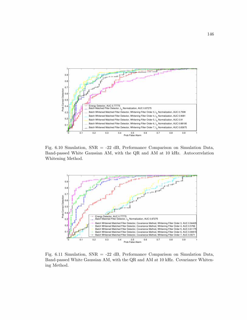
146
0 0.1 0.2 0.3 0.4 0.5 0.6 0.7 0.8 0.9 10
0.1
0.2
0.3
0.4
0.5
0.6
0.7
0.8
0.9
1
Pro
b C
orr
ect D
ete
ction
Prob False Alarm
Energy Detector, AUC 0.77775Batch Matched Filter Detector, L
2 Normalization, AUC 0.87275
Batch Whitened Matched Filter Detector, Whitening Filter Order 3, L2 Normalization, AUC 0.7508
Batch Whitened Matched Filter Detector, Whitening Filter Order 4, L2 Normalization, AUC 0.9081
Batch Whitened Matched Filter Detector, Whitening Filter Order 5, L2 Normalization, AUC 0.91
Batch Whitened Matched Filter Detector, Whitening Filter Order 6, L2 Normalization, AUC 0.88195
Batch Whitened Matched Filter Detector, Whitening Filter Order 7, L2 Normalization, AUC 0.83675
Fig. 6.10 Simulation, SNR = -22 dB, Performance Comparison on Simulation Data,Band-passed White Gaussian AM, with the QR and AM at 10 kHz. AutocorrelationWhitening Method.
0 0.1 0.2 0.3 0.4 0.5 0.6 0.7 0.8 0.9 10
0.1
0.2
0.3
0.4
0.5
0.6
0.7
0.8
0.9
1
Pro
b C
orr
ect D
ete
ction
Prob False Alarm
Energy Detector, AUC 0.77775Batch Matched Filter Detector, L
2 Normalization, AUC 0.87275
Batch Whitened Matched Filter Detector, Covariance Method, Whitening Filter Order 3, AUC 0.94405
Batch Whitened Matched Filter Detector, Covariance Method, Whitening Filter Order 4, AUC 0.5766
Batch Whitened Matched Filter Detector, Covariance Method, Whitening Filter Order 5, AUC 0.61175
Batch Whitened Matched Filter Detector, Covariance Method, Whitening Filter Order 6, AUC 0.90815
Batch Whitened Matched Filter Detector, Covariance Method, Whitening Filter Order 7, AUC 0.5571
Fig. 6.11 Simulation, SNR = -22 dB, Performance Comparison on Simulation Data,Band-passed White Gaussian AM, with the QR and AM at 10 kHz. Covariance Whiten-ing Method.
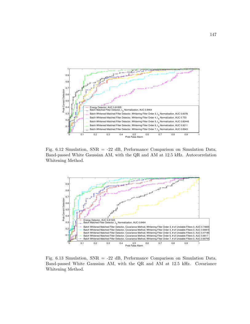
147
0 0.1 0.2 0.3 0.4 0.5 0.6 0.7 0.8 0.9 10
0.1
0.2
0.3
0.4
0.5
0.6
0.7
0.8
0.9
1
Pro
b C
orr
ect D
ete
ction
Prob False Alarm
Energy Detector, AUC 0.81505Batch Matched Filter Detector, L
2 Normalization, AUC 0.8464
Batch Whitened Matched Filter Detector, Whitening Filter Order 3, L2 Normalization, AUC 0.6078
Batch Whitened Matched Filter Detector, Whitening Filter Order 4, L2 Normalization, AUC 0.753
Batch Whitened Matched Filter Detector, Whitening Filter Order 5, L2 Normalization, AUC 0.82445
Batch Whitened Matched Filter Detector, Whitening Filter Order 6, L2 Normalization, AUC 0.9211
Batch Whitened Matched Filter Detector, Whitening Filter Order 7, L2 Normalization, AUC 0.8943
Fig. 6.12 Simulation, SNR = -22 dB, Performance Comparison on Simulation Data,Band-passed White Gaussian AM, with the QR and AM at 12.5 kHz. AutocorrelationWhitening Method.
0 0.1 0.2 0.3 0.4 0.5 0.6 0.7 0.8 0.9 10
0.1
0.2
0.3
0.4
0.5
0.6
0.7
0.8
0.9
1
Pro
b C
orr
ect D
ete
ction
Prob False Alarm
Energy Detector, AUC 0.81505Batch Matched Filter Detector, L
2 Normalization, AUC 0.8464
Batch Whitened Matched Filter Detector, Covariance Method, Whitening Filter Order 3, # of Unstable Filters 0, AUC 0.74655
Batch Whitened Matched Filter Detector, Covariance Method, Whitening Filter Order 4, # of Unstable Filters 0, AUC 0.90815
Batch Whitened Matched Filter Detector, Covariance Method, Whitening Filter Order 5, # of Unstable Filters 0, AUC 0.47185
Batch Whitened Matched Filter Detector, Covariance Method, Whitening Filter Order 6, # of Unstable Filters 0, AUC 0.9017
Batch Whitened Matched Filter Detector, Covariance Method, Whitening Filter Order 7, # of Unstable Filters 0, AUC 0.60755
Fig. 6.13 Simulation, SNR = -22 dB, Performance Comparison on Simulation Data,Band-passed White Gaussian AM, with the QR and AM at 12.5 kHz. CovarianceWhitening Method.
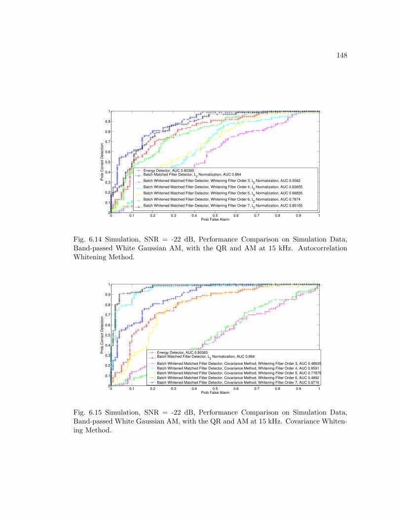
148
0 0.1 0.2 0.3 0.4 0.5 0.6 0.7 0.8 0.9 10
0.1
0.2
0.3
0.4
0.5
0.6
0.7
0.8
0.9
1
Pro
b C
orr
ect D
ete
ction
Prob False Alarm
Energy Detector, AUC 0.80365Batch Matched Filter Detector, L
2 Normalization, AUC 0.884
Batch Whitened Matched Filter Detector, Whitening Filter Order 3, L2 Normalization, AUC 0.5582
Batch Whitened Matched Filter Detector, Whitening Filter Order 4, L2 Normalization, AUC 0.63655
Batch Whitened Matched Filter Detector, Whitening Filter Order 5, L2 Normalization, AUC 0.66835
Batch Whitened Matched Filter Detector, Whitening Filter Order 6, L2 Normalization, AUC 0.7874
Batch Whitened Matched Filter Detector, Whitening Filter Order 7, L2 Normalization, AUC 0.85165
Fig. 6.14 Simulation, SNR = -22 dB, Performance Comparison on Simulation Data,Band-passed White Gaussian AM, with the QR and AM at 15 kHz. AutocorrelationWhitening Method.
0 0.1 0.2 0.3 0.4 0.5 0.6 0.7 0.8 0.9 10
0.1
0.2
0.3
0.4
0.5
0.6
0.7
0.8
0.9
1
Pro
b C
orr
ect D
ete
ction
Prob False Alarm
Energy Detector, AUC 0.80365Batch Matched Filter Detector, L
2 Normalization, AUC 0.884
Batch Whitened Matched Filter Detector, Covariance Method, Whitening Filter Order 3, AUC 0.48635
Batch Whitened Matched Filter Detector, Covariance Method, Whitening Filter Order 4, AUC 0.9591
Batch Whitened Matched Filter Detector, Covariance Method, Whitening Filter Order 5, AUC 0.77875
Batch Whitened Matched Filter Detector, Covariance Method, Whitening Filter Order 6, AUC 0.4892
Batch Whitened Matched Filter Detector, Covariance Method, Whitening Filter Order 7, AUC 0.9716
Fig. 6.15 Simulation, SNR = -22 dB, Performance Comparison on Simulation Data,Band-passed White Gaussian AM, with the QR and AM at 15 kHz. Covariance Whiten-ing Method.
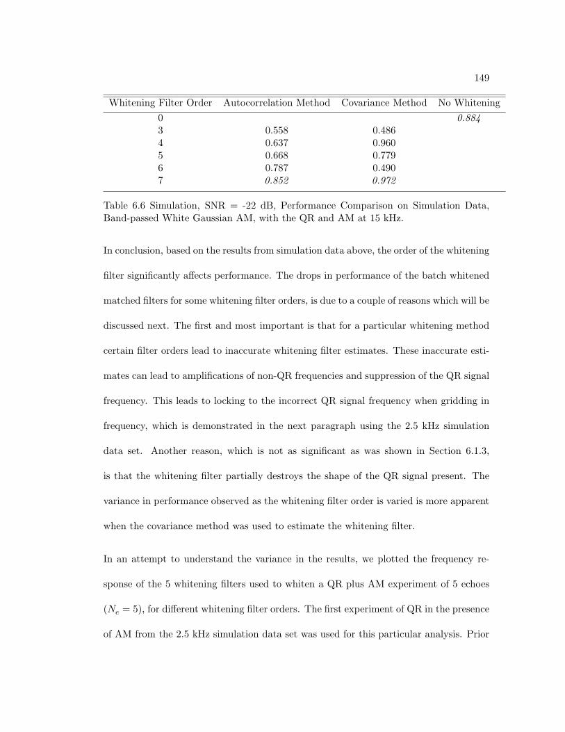
149
Whitening Filter Order Autocorrelation Method Covariance Method No Whitening0 0.8843 0.558 0.4864 0.637 0.9605 0.668 0.7796 0.787 0.4907 0.852 0.972
Table 6.6 Simulation, SNR = -22 dB, Performance Comparison on Simulation Data,Band-passed White Gaussian AM, with the QR and AM at 15 kHz.
In conclusion, based on the results from simulation data above, the order of the whitening
filter significantly affects performance. The drops in performance of the batch whitened
matched filters for some whitening filter orders, is due to a couple of reasons which will be
discussed next. The first and most important is that for a particular whitening method
certain filter orders lead to inaccurate whitening filter estimates. These inaccurate esti-
mates can lead to amplifications of non-QR frequencies and suppression of the QR signal
frequency. This leads to locking to the incorrect QR signal frequency when gridding in
frequency, which is demonstrated in the next paragraph using the 2.5 kHz simulation
data set. Another reason, which is not as significant as was shown in Section 6.1.3,
is that the whitening filter partially destroys the shape of the QR signal present. The
variance in performance observed as the whitening filter order is varied is more apparent
when the covariance method was used to estimate the whitening filter.
In an attempt to understand the variance in the results, we plotted the frequency re-
sponse of the 5 whitening filters used to whiten a QR plus AM experiment of 5 echoes
(Ne = 5), for different whitening filter orders. The first experiment of QR in the presence
of AM from the 2.5 kHz simulation data set was used for this particular analysis. Prior
150
to plotting the whitening filters for different filter orders, we plotted what we expect
the frequency response in theory of a whitening filter to look like. To whiten an AM
signal, the whitening filter’s frequency response should be the inverse of the AM signal’s
frequency response. A bandpassed white gaussian AM signal with a carrier at 2.5 kHz,
which is less than the upper cutoff frequency of the bandpass filter (10 kHz) has over-
lapping sidebands, which lead to an uneven frequency spectrum. Figure (6.16) displays
the frequency response of the bandpassed white gaussian noise, while the bottom part
displays the frequency response of the bandpassed white gaussian AM signal. Therefore
in theory we would expect the whitening filter’s frequency spectrum to be the inverse of
the frequency spectrum of the AM signal, shown in the bottom of Figure (6.17). The
spectrum of the whitening filter in theory should try to equally amplify the frequency
bands 2.46 kHz-2.54 kHz and 7.5 kHz-12.5 kHz. The filter should also provide a larger
amplification of the frequencies greater than 12.5 kHz, while suppressing the remaining
frequencies.
To compare the frequency response of the whitening filter we expect in theory to the
frequency responses observed in experiment, the responses of the whitening filters for
filter orders 3-7 for both design methods were plotted. The frequency response of the
5 whitening filters (one for each echo of the experiment) designed using the covariance
method for filter orders 3-7 are shown in Figures (6.19)-(6.23) respectively. The spec-
trums of the 5 whitening filters (all-zero filters) of a particular order are overlaid in a
single figure along with the frequencies the filter’s zeros correspond to. The angle be-
tween the location of the zero and the positive real axis is what determines this frequency.
151
All filters attempt to mimic the expected whitening filter but some are limited by the
number of zeros (filter order).
Comparing these figures shows that the closest match between the expected whitening
filter and the whitening filters observed occurs when the filter order used is of 7th or-
der. The spectrum of the whitening filters of 4th and 6th order in Figure (6.20) also
closely resembles the spectrum of the whitening filter in theory, with the exception of
not suppressing the frequencies below 2.46 kHz. Therefore one expects these filter orders
to lead to good performance. Figures (6.19) and (6.21) clearly show that the whitening
filters of orders 3 and 5 suppress the QR signal’s frequency (2.5 kHz) when compared
to other frequencies. These filter estimates attempt to suppress the 0-2.46 kHz band
by placing one of the filter’s zeros on the positive real axis, which corresponds to the
zero frequency. The magnitude of frequency response of the filters should then rise at
2.46 kHz to follow the whitening filter in theory but does not rise fast enough to prevent
a suppression of the 2.5 kHz QR signal frequency, whose spectrum is shown in Figure
(6.18). This phenomena leads to the filter often locking to incorrect frequencies when
gridding. This does not occur with the 7th order filter due to the increase in the model
order, which increases the maneuverability of the frequency response.
The filter estimates of even order, 4 and 6, place the zeros in complex conjugates to
suppress higher frequencies since placing a zero on the positive real axis to suppress
the 0-2.46 kHz frequency band limits another zero to a non-complex value. Since these
whitening filter estimates do not attempt to suppress the 0-2.46 kHz frequency band, the
QR signal’s frequency of 2.5 kHz is not suppressed in the same manner as when a 3rd
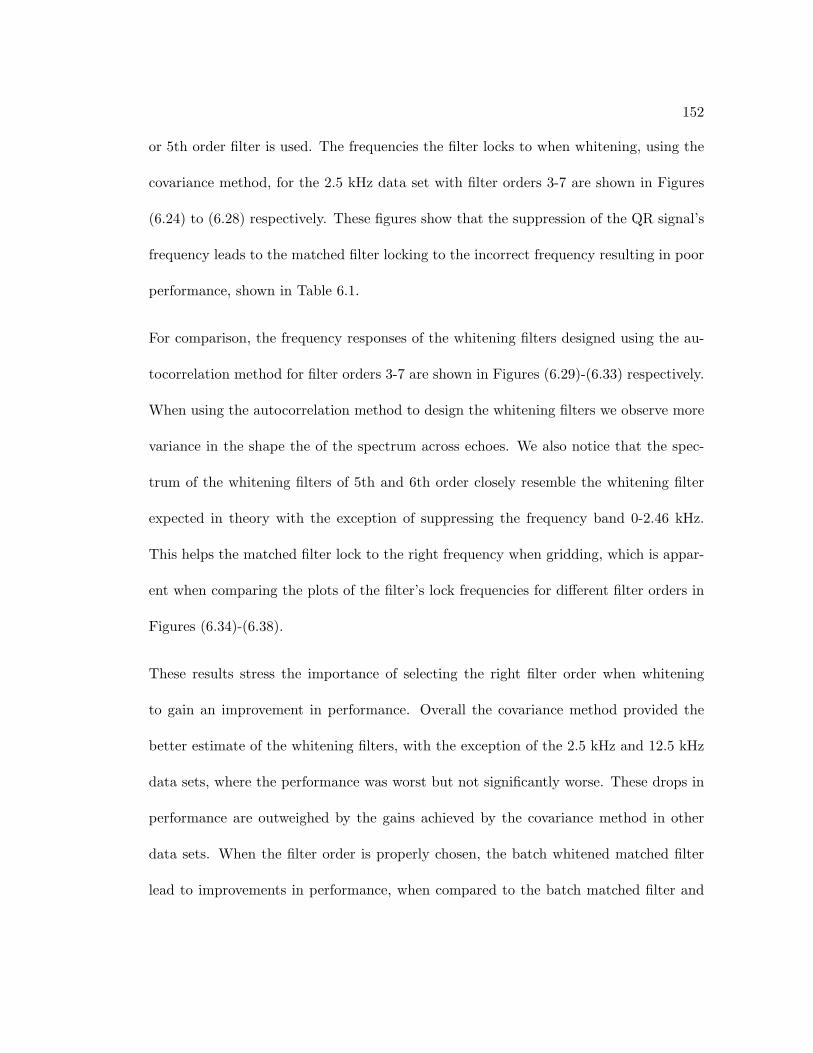
152
or 5th order filter is used. The frequencies the filter locks to when whitening, using the
covariance method, for the 2.5 kHz data set with filter orders 3-7 are shown in Figures
(6.24) to (6.28) respectively. These figures show that the suppression of the QR signal’s
frequency leads to the matched filter locking to the incorrect frequency resulting in poor
performance, shown in Table 6.1.
For comparison, the frequency responses of the whitening filters designed using the au-
tocorrelation method for filter orders 3-7 are shown in Figures (6.29)-(6.33) respectively.
When using the autocorrelation method to design the whitening filters we observe more
variance in the shape the of the spectrum across echoes. We also notice that the spec-
trum of the whitening filters of 5th and 6th order closely resemble the whitening filter
expected in theory with the exception of suppressing the frequency band 0-2.46 kHz.
This helps the matched filter lock to the right frequency when gridding, which is appar-
ent when comparing the plots of the filter’s lock frequencies for different filter orders in
Figures (6.34)-(6.38).
These results stress the importance of selecting the right filter order when whitening
to gain an improvement in performance. Overall the covariance method provided the
better estimate of the whitening filters, with the exception of the 2.5 kHz and 12.5 kHz
data sets, where the performance was worst but not significantly worse. These drops in
performance are outweighed by the gains achieved by the covariance method in other
data sets. When the filter order is properly chosen, the batch whitened matched filter
lead to improvements in performance, when compared to the batch matched filter and
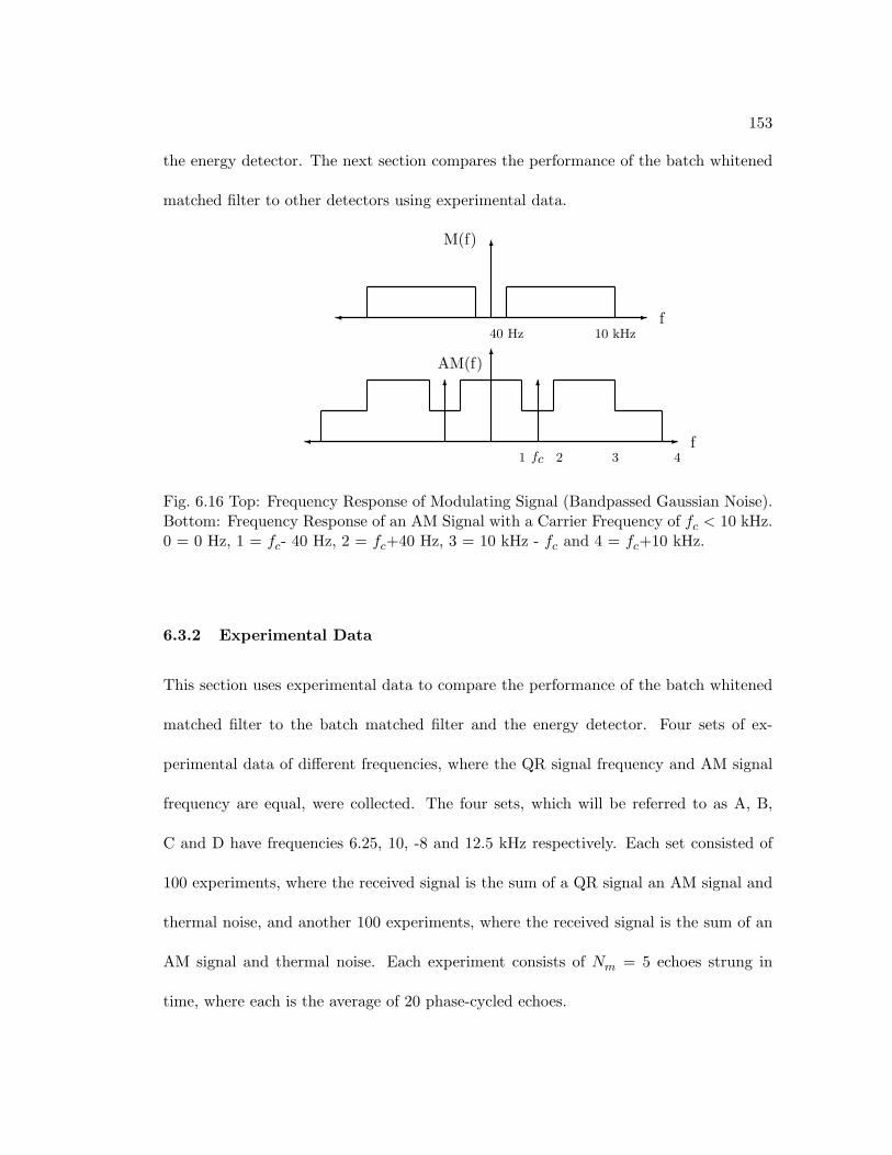
153
the energy detector. The next section compares the performance of the batch whitened
matched filter to other detectors using experimental data.
6
-�
6
-�
6
M(f)
AM(f)
6
40 Hz 10 kHz
fc 4321
f
f
Fig. 6.16 Top: Frequency Response of Modulating Signal (Bandpassed Gaussian Noise).Bottom: Frequency Response of an AM Signal with a Carrier Frequency of fc < 10 kHz.0 = 0 Hz, 1 = fc- 40 Hz, 2 = fc+40 Hz, 3 = 10 kHz - fc and 4 = fc+10 kHz.
6.3.2 Experimental Data
This section uses experimental data to compare the performance of the batch whitened
matched filter to the batch matched filter and the energy detector. Four sets of ex-
perimental data of different frequencies, where the QR signal frequency and AM signal
frequency are equal, were collected. The four sets, which will be referred to as A, B,
C and D have frequencies 6.25, 10, -8 and 12.5 kHz respectively. Each set consisted of
100 experiments, where the received signal is the sum of a QR signal an AM signal and
thermal noise, and another 100 experiments, where the received signal is the sum of an
AM signal and thermal noise. Each experiment consists of Nm = 5 echoes strung in
time, where each is the average of 20 phase-cycled echoes.
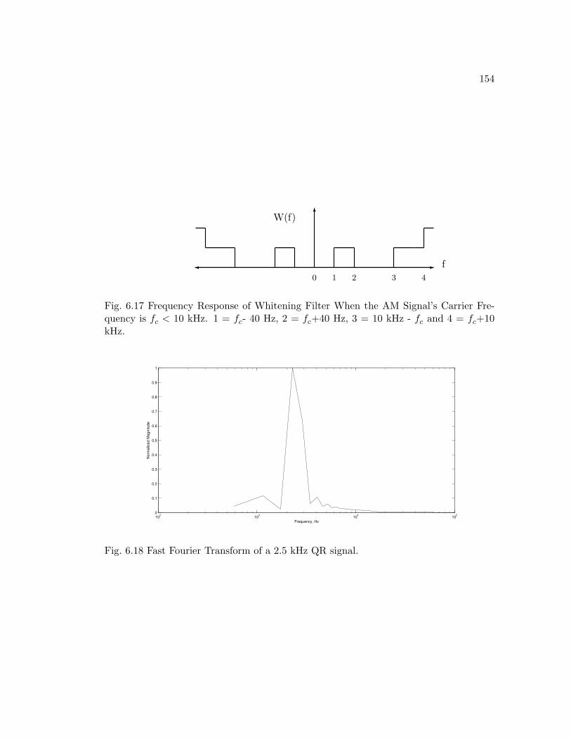
154
-�
6
f
W(f)
0 1 2 3 4
Fig. 6.17 Frequency Response of Whitening Filter When the AM Signal’s Carrier Fre-quency is fc < 10 kHz. 1 = fc- 40 Hz, 2 = fc+40 Hz, 3 = 10 kHz - fc and 4 = fc+10kHz.
102
103
104
105
0
0.1
0.2
0.3
0.4
0.5
0.6
0.7
0.8
0.9
1
Frequency, Hz
Norm
aliz
ed M
agnitude
Fig. 6.18 Fast Fourier Transform of a 2.5 kHz QR signal.
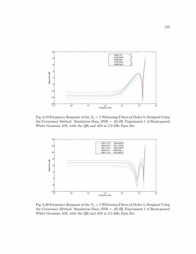
155
10−1
100
101
102
103
104
105
−20
−15
−10
−5
0
5
10
15
20
Frequency (Hz)
Magnitude (
dB
)
15940.776 0
16052.9356 0
15588.996 0
15790.9769 0
16852.9618 0
Fig. 6.19 Frequency Response of the Ne = 5 Whitening Filters of Order 3, Designed Usingthe Covariance Method. Simulation Data, SNR = -22 dB, Experiment 1 of Band-passedWhite Gaussian AM, with the QR and AM at 2.5 kHz Data Set.
10−1
100
101
102
103
104
105
−10
−5
0
5
10
15
20
25
30
Frequency (Hz)
Magnitude (
dB
)
18312.1716 7948.42976
18546.3477 7521.10352
18317.2419 7300.70097
18942.616 7699.4048
18831.1747 6767.84707
Fig. 6.20 Frequency Response of the Ne = 5 Whitening Filters of Order 4, Designed Usingthe Covariance Method. Simulation Data, SNR = -22 dB, Experiment 1 of Band-passedWhite Gaussian AM, with the QR and AM at 2.5 kHz Data Set.
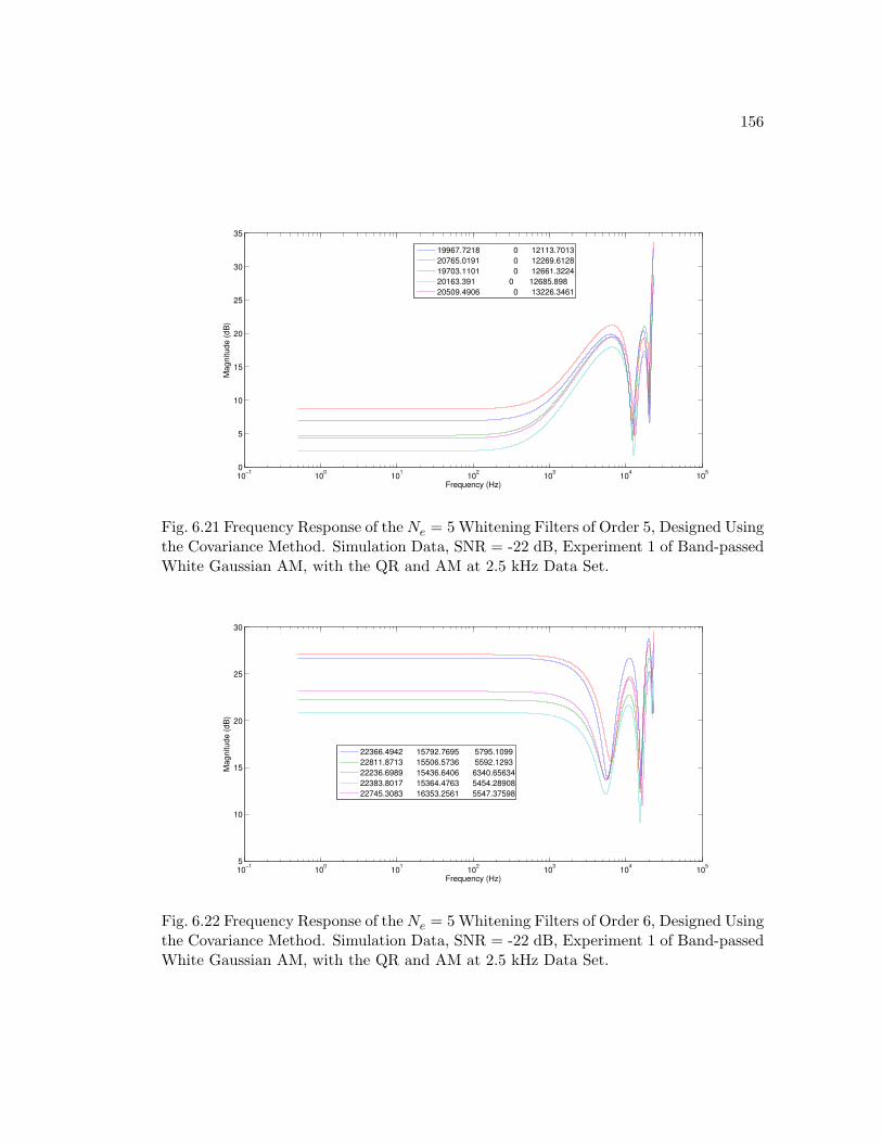
156
10−1
100
101
102
103
104
105
0
5
10
15
20
25
30
35
Frequency (Hz)
Magnitude (
dB
)
19967.7218 0 12113.7013
20765.0191 0 12269.6128
19703.1101 0 12661.3224
20163.391 0 12685.898
20509.4906 0 13226.3461
Fig. 6.21 Frequency Response of the Ne = 5 Whitening Filters of Order 5, Designed Usingthe Covariance Method. Simulation Data, SNR = -22 dB, Experiment 1 of Band-passedWhite Gaussian AM, with the QR and AM at 2.5 kHz Data Set.
10−1
100
101
102
103
104
105
5
10
15
20
25
30
Frequency (Hz)
Magnitude (
dB
)
22366.4942 15792.7695 5795.1099
22811.8713 15506.5736 5592.1293
22236.6989 15436.6406 6340.65634
22383.8017 15364.4763 5454.28908
22745.3083 16353.2561 5547.37598
Fig. 6.22 Frequency Response of the Ne = 5 Whitening Filters of Order 6, Designed Usingthe Covariance Method. Simulation Data, SNR = -22 dB, Experiment 1 of Band-passedWhite Gaussian AM, with the QR and AM at 2.5 kHz Data Set.
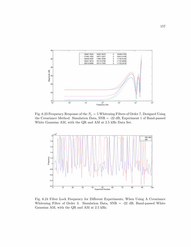
157
10−1
100
101
102
103
104
105
15
20
25
30
35
40
45
Frequency (Hz)
Magnitude (
dB
)
25687.0526 18087.6676 0 10048.4705
27492.1822 19071.2527 0 10912.4108
26548.0555 17897.4936 0 11100.8156
26301.9618 18174.9786 0 11103.9658
26519.6586 18713.7305 0 11153.2078
Fig. 6.23 Frequency Response of the Ne = 5 Whitening Filters of Order 7, Designed Usingthe Covariance Method. Simulation Data, SNR = -22 dB, Experiment 1 of Band-passedWhite Gaussian AM, with the QR and AM at 2.5 kHz Data Set.
0 10 20 30 40 50 60 70 80 90 1000.2
0.4
0.6
0.8
1
1.2
1.4
1.6
1.8
2x 10
4
Experiment Number
Fre
quency
QR+AM
AM
Fig. 6.24 Filter Lock Frequency for Different Experiments, When Using A CovarianceWhitening Filter of Order 3. Simulation Data, SNR = -22 dB, Band-passed WhiteGaussian AM, with the QR and AM at 2.5 kHz.
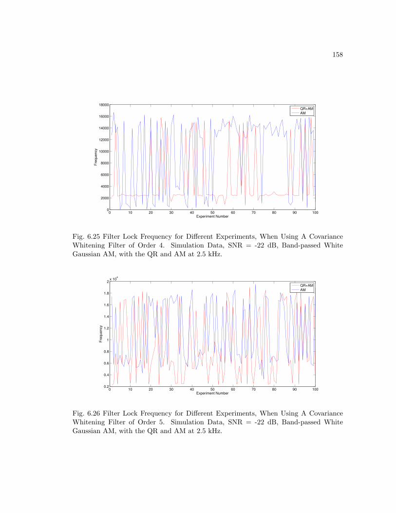
158
0 10 20 30 40 50 60 70 80 90 1000
2000
4000
6000
8000
10000
12000
14000
16000
18000
Experiment Number
Fre
quency
QR+AM
AM
Fig. 6.25 Filter Lock Frequency for Different Experiments, When Using A CovarianceWhitening Filter of Order 4. Simulation Data, SNR = -22 dB, Band-passed WhiteGaussian AM, with the QR and AM at 2.5 kHz.
0 10 20 30 40 50 60 70 80 90 1000.2
0.4
0.6
0.8
1
1.2
1.4
1.6
1.8
2x 10
4
Experiment Number
Fre
quency
QR+AM
AM
Fig. 6.26 Filter Lock Frequency for Different Experiments, When Using A CovarianceWhitening Filter of Order 5. Simulation Data, SNR = -22 dB, Band-passed WhiteGaussian AM, with the QR and AM at 2.5 kHz.
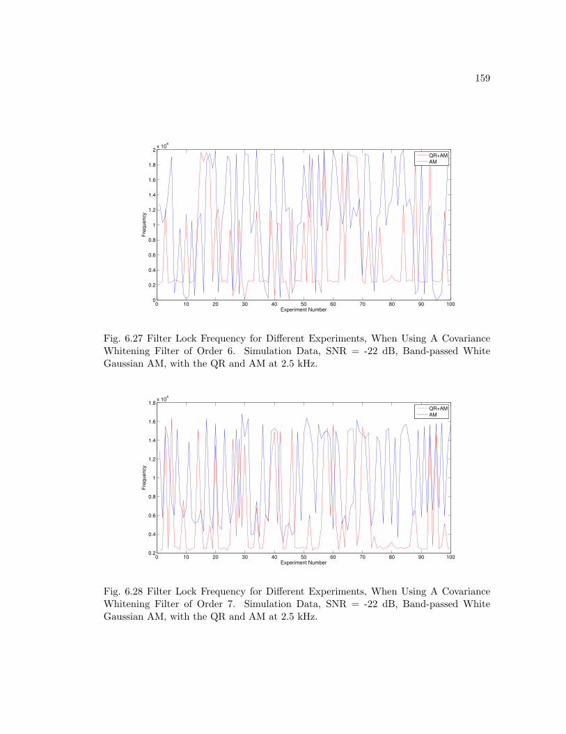
159
0 10 20 30 40 50 60 70 80 90 1000
0.2
0.4
0.6
0.8
1
1.2
1.4
1.6
1.8
2x 10
4
Experiment Number
Fre
quency
QR+AM
AM
Fig. 6.27 Filter Lock Frequency for Different Experiments, When Using A CovarianceWhitening Filter of Order 6. Simulation Data, SNR = -22 dB, Band-passed WhiteGaussian AM, with the QR and AM at 2.5 kHz.
0 10 20 30 40 50 60 70 80 90 1000.2
0.4
0.6
0.8
1
1.2
1.4
1.6
1.8x 10
4
Experiment Number
Fre
quency
QR+AM
AM
Fig. 6.28 Filter Lock Frequency for Different Experiments, When Using A CovarianceWhitening Filter of Order 7. Simulation Data, SNR = -22 dB, Band-passed WhiteGaussian AM, with the QR and AM at 2.5 kHz.
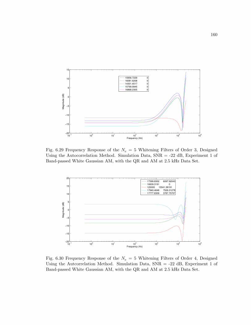
160
10−1
100
101
102
103
104
105
−20
−15
−10
−5
0
5
10
15
Frequency (Hz)
Magnitude (
dB
)
15956.7229 0
16081.6208 0
14301.4517 0
15799.9945 0
16868.2305 0
Fig. 6.29 Frequency Response of the Ne = 5 Whitening Filters of Order 3, DesignedUsing the Autocorrelation Method. Simulation Data, SNR = -22 dB, Experiment 1 ofBand-passed White Gaussian AM, with the QR and AM at 2.5 kHz Data Set.
10−1
100
101
102
103
104
105
−20
−15
−10
−5
0
5
10
15
20
Frequency (Hz)
Magnitude (
dB
)
17399.8302 6097.92043
16609.3191 0
125000 15541.38191
17940.4648 7526.31278
17777.8309 3787.75707
Fig. 6.30 Frequency Response of the Ne = 5 Whitening Filters of Order 4, DesignedUsing the Autcorrelation Method. Simulation Data, SNR = -22 dB, Experiment 1 ofBand-passed White Gaussian AM, with the QR and AM at 2.5 kHz Data Set.
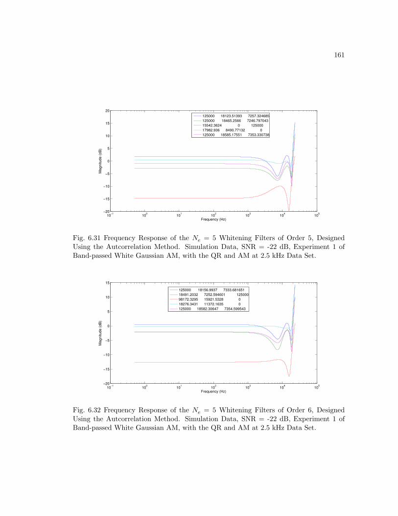
161
10−1
100
101
102
103
104
105
−20
−15
−10
−5
0
5
10
15
20
Frequency (Hz)
Magnitude (
dB
)
125000 18123.51393 7257.324685
125000 18465.2566 7246.797043
15542.3624 0 125000
17982.936 8490.77132 0
125000 18585.17551 7353.330738
Fig. 6.31 Frequency Response of the Ne = 5 Whitening Filters of Order 5, DesignedUsing the Autcorrelation Method. Simulation Data, SNR = -22 dB, Experiment 1 ofBand-passed White Gaussian AM, with the QR and AM at 2.5 kHz Data Set.
10−1
100
101
102
103
104
105
−20
−15
−10
−5
0
5
10
15
Frequency (Hz)
Magnitude (
dB
)
125000 18156.9937 7333.681651
18491.2032 7252.594601 125000
98172.3295 15921.5328 0
18276.3431 11372.1635 0
125000 18582.30647 7354.599543
Fig. 6.32 Frequency Response of the Ne = 5 Whitening Filters of Order 6, DesignedUsing the Autcorrelation Method. Simulation Data, SNR = -22 dB, Experiment 1 ofBand-passed White Gaussian AM, with the QR and AM at 2.5 kHz Data Set.
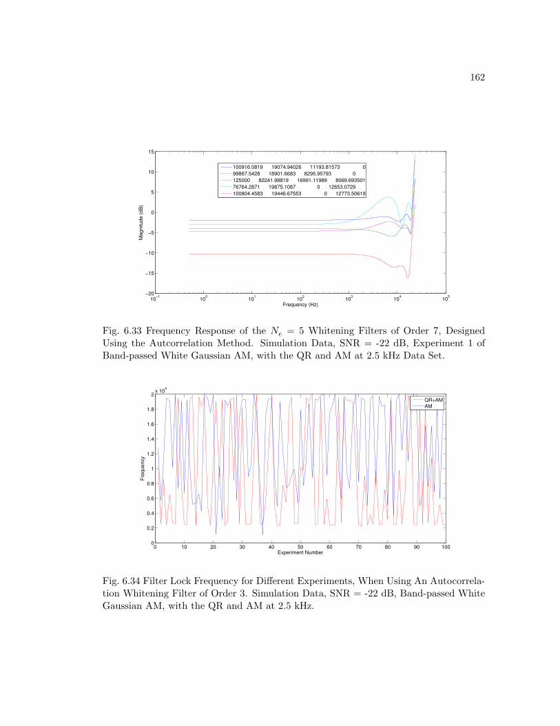
162
10−1
100
101
102
103
104
105
−20
−15
−10
−5
0
5
10
15
Frequency (Hz)
Magnitude (
dB
)
100916.0819 19074.94026 11193.81573 0
99867.5428 18901.6683 8295.95793 0
125000 82241.98819 16991.11989 8069.693501
76764.2871 19875.1087 0 12653.0729
100804.4583 19446.67553 0 12773.50619
Fig. 6.33 Frequency Response of the Ne = 5 Whitening Filters of Order 7, DesignedUsing the Autcorrelation Method. Simulation Data, SNR = -22 dB, Experiment 1 ofBand-passed White Gaussian AM, with the QR and AM at 2.5 kHz Data Set.
0 10 20 30 40 50 60 70 80 90 1000
0.2
0.4
0.6
0.8
1
1.2
1.4
1.6
1.8
2x 10
4
Experiment Number
Fre
quency
QR+AM
AM
Fig. 6.34 Filter Lock Frequency for Different Experiments, When Using An Autocorrela-tion Whitening Filter of Order 3. Simulation Data, SNR = -22 dB, Band-passed WhiteGaussian AM, with the QR and AM at 2.5 kHz.
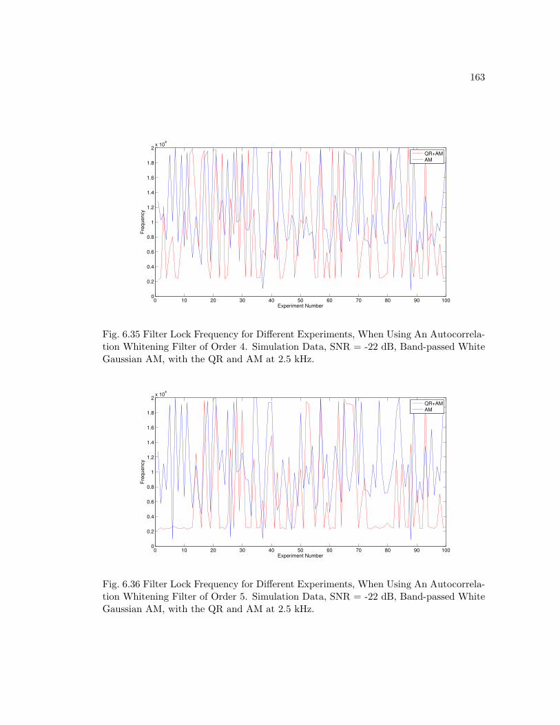
163
0 10 20 30 40 50 60 70 80 90 1000
0.2
0.4
0.6
0.8
1
1.2
1.4
1.6
1.8
2x 10
4
Experiment Number
Fre
quency
QR+AM
AM
Fig. 6.35 Filter Lock Frequency for Different Experiments, When Using An Autocorrela-tion Whitening Filter of Order 4. Simulation Data, SNR = -22 dB, Band-passed WhiteGaussian AM, with the QR and AM at 2.5 kHz.
0 10 20 30 40 50 60 70 80 90 1000
0.2
0.4
0.6
0.8
1
1.2
1.4
1.6
1.8
2x 10
4
Experiment Number
Fre
quency
QR+AM
AM
Fig. 6.36 Filter Lock Frequency for Different Experiments, When Using An Autocorrela-tion Whitening Filter of Order 5. Simulation Data, SNR = -22 dB, Band-passed WhiteGaussian AM, with the QR and AM at 2.5 kHz.
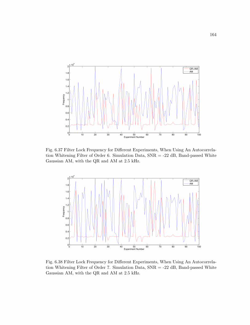
164
0 10 20 30 40 50 60 70 80 90 1000
0.2
0.4
0.6
0.8
1
1.2
1.4
1.6
1.8
2x 10
4
Experiment Number
Fre
quency
QR+AM
AM
Fig. 6.37 Filter Lock Frequency for Different Experiments, When Using An Autocorrela-tion Whitening Filter of Order 6. Simulation Data, SNR = -22 dB, Band-passed WhiteGaussian AM, with the QR and AM at 2.5 kHz.
0 10 20 30 40 50 60 70 80 90 1000
0.2
0.4
0.6
0.8
1
1.2
1.4
1.6
1.8
2x 10
4
Experiment Number
Fre
quency
QR+AM
AM
Fig. 6.38 Filter Lock Frequency for Different Experiments, When Using An Autocorrela-tion Whitening Filter of Order 7. Simulation Data, SNR = -22 dB, Band-passed WhiteGaussian AM, with the QR and AM at 2.5 kHz.
165
The batch matched filter grid parameters are provided in section 5.3.2 and therefore are
not repeated here. The batch whitened match filter on the other hand, for both the
autocorrelation and the covariance whitening methods with the different whitening filter
orders, used the following values to grid, ωlb = 0, ωub = 40000π, ω∆ = 200π, φ∆ = .1,
T ∗2 lb
= 300e − 6, T ∗2 ub
= 500e − 6 and T ∗2 ∆
= 100e − 6. The above values lead to
Ndf = 201, Ndφ = 63 and NdT = 3 in each of the three dimensions, which corresponds
to Ndf × Ndφ × NdT = 37989 filters in the batch. Again the number of filters in the
batch was reduced, when compared to the batch matched filter, due to the increase in
computation time per filter. The increase in computation time is due to having to whiten
each filter in the batch, with the Nm filters. A finer grid, leading to an increase in the
number of filters in the batch, may lead to a slight increase in performance. Though the
effect of finer gridding on performance was discussed in Section and therefore will not
be discussed here.
ROC plots were used to compare the performance of the batch whitened matched filter
to the batch matched filter and the energy detector using four different experimental
setups. Figures (6.39-6.46) compare the performance of the different detectors for the
different experimental setups. As with the simulation data, each figure compares the
energy detector and the batch matched filter to the batch whitened matched filter, using
either the autocorrelation or the covariance method, as the whitening filter order is
varied.
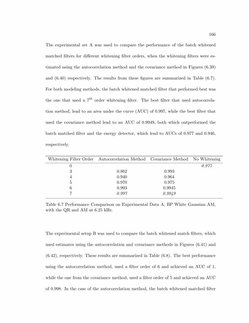
166
The experimental set A was used to compare the performance of the batch whitened
matched filters for different whitening filter orders, when the whitening filters were es-
timated using the autocorrelation method and the covariance method in Figures (6.39)
and (6.40) respectively. The results from these figures are summarized in Table (6.7).
For both modeling methods, the batch whitened matched filter that performed best was
the one that used a 7th order whitening filter. The best filter that used autocorrela-
tion method, lead to an area under the curve (AUC) of 0.997, while the best filter that
used the covariance method lead to an AUC of 0.9949, both which outperformed the
batch matched filter and the energy detector, which lead to AUCs of 0.977 and 0.946,
respectively.
Whitening Filter Order Autocorrelation Method Covariance Method No Whitening0 0.9773 0.862 0.9934 0.940 0.9645 0.970 0.9756 0.993 0.99457 0.997 0.9949
Table 6.7 Performance Comparison on Experimental Data A, BP White Gaussian AM,with the QR and AM at 6.25 kHz.
The experimental setup B was used to compare the batch whitened match filters, which
used estimates using the autocorrelation and covariance methods in Figures (6.41) and
(6.42), respectively. These results are summarized in Table (6.8). The best performance
using the autocorrelation method, used a filter order of 6 and achieved an AUC of 1,
while the one from the covariance method, used a filter order of 5 and achieved an AUC
of 0.998. In the case of the autocorrelation method, the batch whitened matched filter
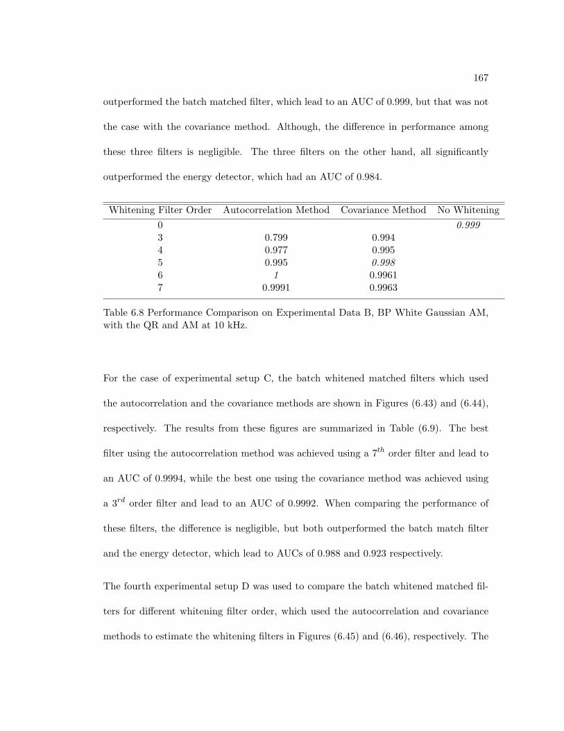
167
outperformed the batch matched filter, which lead to an AUC of 0.999, but that was not
the case with the covariance method. Although, the difference in performance among
these three filters is negligible. The three filters on the other hand, all significantly
outperformed the energy detector, which had an AUC of 0.984.
Whitening Filter Order Autocorrelation Method Covariance Method No Whitening0 0.9993 0.799 0.9944 0.977 0.9955 0.995 0.9986 1 0.99617 0.9991 0.9963
Table 6.8 Performance Comparison on Experimental Data B, BP White Gaussian AM,with the QR and AM at 10 kHz.
For the case of experimental setup C, the batch whitened matched filters which used
the autocorrelation and the covariance methods are shown in Figures (6.43) and (6.44),
respectively. The results from these figures are summarized in Table (6.9). The best
filter using the autocorrelation method was achieved using a 7th order filter and lead to
an AUC of 0.9994, while the best one using the covariance method was achieved using
a 3rd order filter and lead to an AUC of 0.9992. When comparing the performance of
these filters, the difference is negligible, but both outperformed the batch match filter
and the energy detector, which lead to AUCs of 0.988 and 0.923 respectively.
The fourth experimental setup D was used to compare the batch whitened matched fil-
ters for different whitening filter order, which used the autocorrelation and covariance
methods to estimate the whitening filters in Figures (6.45) and (6.46), respectively. The
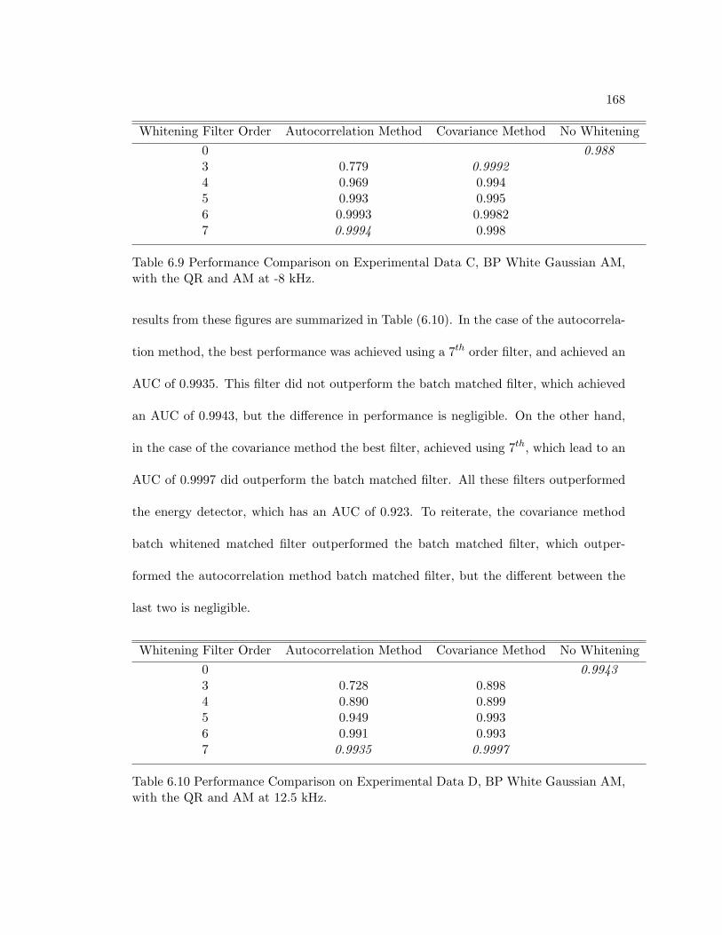
168
Whitening Filter Order Autocorrelation Method Covariance Method No Whitening0 0.9883 0.779 0.99924 0.969 0.9945 0.993 0.9956 0.9993 0.99827 0.9994 0.998
Table 6.9 Performance Comparison on Experimental Data C, BP White Gaussian AM,with the QR and AM at -8 kHz.
results from these figures are summarized in Table (6.10). In the case of the autocorrela-
tion method, the best performance was achieved using a 7th order filter, and achieved an
AUC of 0.9935. This filter did not outperform the batch matched filter, which achieved
an AUC of 0.9943, but the difference in performance is negligible. On the other hand,
in the case of the covariance method the best filter, achieved using 7th, which lead to an
AUC of 0.9997 did outperform the batch matched filter. All these filters outperformed
the energy detector, which has an AUC of 0.923. To reiterate, the covariance method
batch whitened matched filter outperformed the batch matched filter, which outper-
formed the autocorrelation method batch matched filter, but the different between the
last two is negligible.
Whitening Filter Order Autocorrelation Method Covariance Method No Whitening0 0.99433 0.728 0.8984 0.890 0.8995 0.949 0.9936 0.991 0.9937 0.9935 0.9997
Table 6.10 Performance Comparison on Experimental Data D, BP White Gaussian AM,with the QR and AM at 12.5 kHz.

169
In the following cases: experiment B (covariance method), experiment D (autocorre-
lation), the best performing batch whitened matched filter performs worse than batch
matched filter. Though, the difference in performance is negligible, especially when com-
pared to the gains in performance achieved by the whitening approach in other cases.
In conclusion, the best performing batch whitened matched filter, for both the autocor-
relation and the covariance method, either outperforms or achieves approximately equal
performance, when compared to the batch matched filter.
0 0.1 0.2 0.3 0.4 0.5 0.6 0.7 0.8 0.9 10
0.1
0.2
0.3
0.4
0.5
0.6
0.7
0.8
0.9
1
Pro
b C
orr
ect D
ete
ction
Prob False Alarm
Energy Detector, AUC 0.9455Batch Matched Filter Detector, L
2 Normalization, AUC 0.97745
Batch Whitened Matched Filter Detector, Whitening Filter Order 3, L2 Normalization, AUC 0.8616
Batch Whitened Matched Filter Detector, Whitening Filter Order 4, L2 Normalization, AUC 0.9401
Batch Whitened Matched Filter Detector, Whitening Filter Order 5, L2 Normalization, AUC 0.9691
Batch Whitened Matched Filter Detector, Whitening Filter Order 6, L2 Normalization, AUC 0.9927
Batch Whitened Matched Filter Detector, Whitening Filter Order 7, L2 Normalization, AUC 0.997
Fig. 6.39 Performance Comparison on Experiment Data, BP White Gaussian AM, withthe QR and AM at 6.25 kHz. Autocorrelation Method.
6.4 Batch Adaptive Whitened Matched Filter
This section introduces two adaptive ways to choosing the whitening filter order that can
be applied when modeling with both the autocorrelation and covariance methods. The
first is a method that selects the whitening filter order that least affects the estimated QR
signal intended to match the QR signal present, had one been present. The second selects
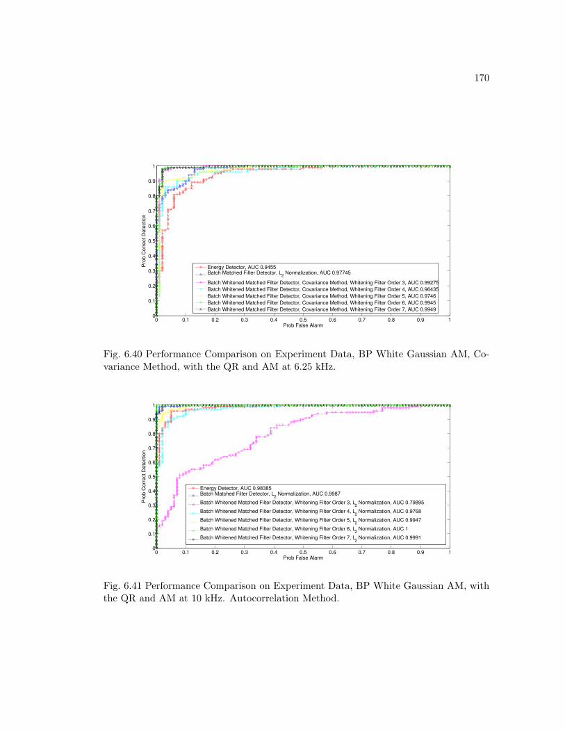
170
0 0.1 0.2 0.3 0.4 0.5 0.6 0.7 0.8 0.9 10
0.1
0.2
0.3
0.4
0.5
0.6
0.7
0.8
0.9
1
Pro
b C
orr
ect D
ete
ction
Prob False Alarm
Energy Detector, AUC 0.9455Batch Matched Filter Detector, L
2 Normalization, AUC 0.97745
Batch Whitened Matched Filter Detector, Covariance Method, Whitening Filter Order 3, AUC 0.99275
Batch Whitened Matched Filter Detector, Covariance Method, Whitening Filter Order 4, AUC 0.96435
Batch Whitened Matched Filter Detector, Covariance Method, Whitening Filter Order 5, AUC 0.9746
Batch Whitened Matched Filter Detector, Covariance Method, Whitening Filter Order 6, AUC 0.9945
Batch Whitened Matched Filter Detector, Covariance Method, Whitening Filter Order 7, AUC 0.9949
Fig. 6.40 Performance Comparison on Experiment Data, BP White Gaussian AM, Co-variance Method, with the QR and AM at 6.25 kHz.
0 0.1 0.2 0.3 0.4 0.5 0.6 0.7 0.8 0.9 10
0.1
0.2
0.3
0.4
0.5
0.6
0.7
0.8
0.9
1
Pro
b C
orr
ect D
ete
ction
Prob False Alarm
Energy Detector, AUC 0.98385Batch Matched Filter Detector, L
2 Normalization, AUC 0.9987
Batch Whitened Matched Filter Detector, Whitening Filter Order 3, L2 Normalization, AUC 0.79895
Batch Whitened Matched Filter Detector, Whitening Filter Order 4, L2 Normalization, AUC 0.9768
Batch Whitened Matched Filter Detector, Whitening Filter Order 5, L2 Normalization, AUC 0.9947
Batch Whitened Matched Filter Detector, Whitening Filter Order 6, L2 Normalization, AUC 1
Batch Whitened Matched Filter Detector, Whitening Filter Order 7, L2 Normalization, AUC 0.9991
Fig. 6.41 Performance Comparison on Experiment Data, BP White Gaussian AM, withthe QR and AM at 10 kHz. Autocorrelation Method.
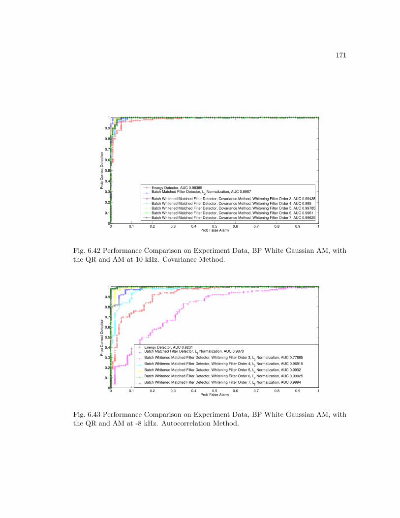
171
0 0.1 0.2 0.3 0.4 0.5 0.6 0.7 0.8 0.9 10
0.1
0.2
0.3
0.4
0.5
0.6
0.7
0.8
0.9
1
Pro
b C
orr
ect D
ete
ction
Prob False Alarm
Energy Detector, AUC 0.98385Batch Matched Filter Detector, L
2 Normalization, AUC 0.9987
Batch Whitened Matched Filter Detector, Covariance Method, Whitening Filter Order 3, AUC 0.99435
Batch Whitened Matched Filter Detector, Covariance Method, Whitening Filter Order 4, AUC 0.995
Batch Whitened Matched Filter Detector, Covariance Method, Whitening Filter Order 5, AUC 0.99785
Batch Whitened Matched Filter Detector, Covariance Method, Whitening Filter Order 6, AUC 0.9961
Batch Whitened Matched Filter Detector, Covariance Method, Whitening Filter Order 7, AUC 0.99625
Fig. 6.42 Performance Comparison on Experiment Data, BP White Gaussian AM, withthe QR and AM at 10 kHz. Covariance Method.
0 0.1 0.2 0.3 0.4 0.5 0.6 0.7 0.8 0.9 10
0.1
0.2
0.3
0.4
0.5
0.6
0.7
0.8
0.9
1
Pro
b C
orr
ect D
ete
ction
Prob False Alarm
Energy Detector, AUC 0.9231Batch Matched Filter Detector, L
2 Normalization, AUC 0.9878
Batch Whitened Matched Filter Detector, Whitening Filter Order 3, L2 Normalization, AUC 0.77885
Batch Whitened Matched Filter Detector, Whitening Filter Order 4, L2 Normalization, AUC 0.96915
Batch Whitened Matched Filter Detector, Whitening Filter Order 5, L2 Normalization, AUC 0.9932
Batch Whitened Matched Filter Detector, Whitening Filter Order 6, L2 Normalization, AUC 0.99925
Batch Whitened Matched Filter Detector, Whitening Filter Order 7, L2 Normalization, AUC 0.9994
Fig. 6.43 Performance Comparison on Experiment Data, BP White Gaussian AM, withthe QR and AM at -8 kHz. Autocorrelation Method.
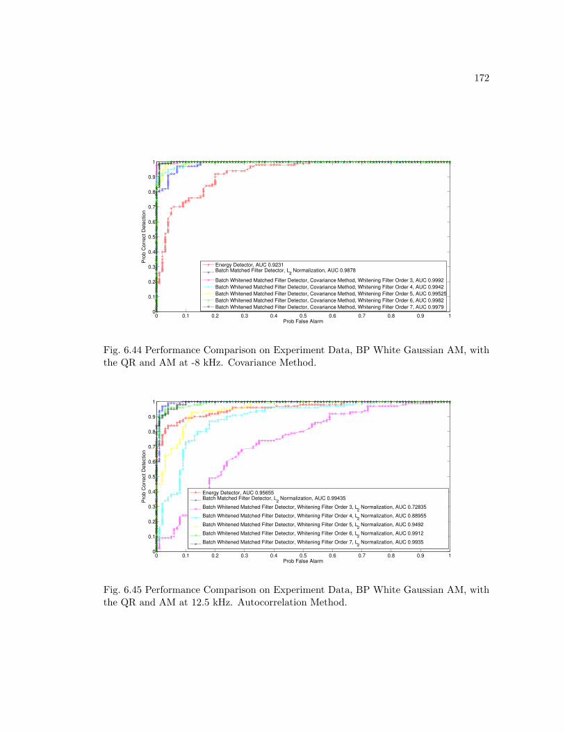
172
0 0.1 0.2 0.3 0.4 0.5 0.6 0.7 0.8 0.9 10
0.1
0.2
0.3
0.4
0.5
0.6
0.7
0.8
0.9
1
Pro
b C
orr
ect D
ete
ction
Prob False Alarm
Energy Detector, AUC 0.9231Batch Matched Filter Detector, L
2 Normalization, AUC 0.9878
Batch Whitened Matched Filter Detector, Covariance Method, Whitening Filter Order 3, AUC 0.9992
Batch Whitened Matched Filter Detector, Covariance Method, Whitening Filter Order 4, AUC 0.9942
Batch Whitened Matched Filter Detector, Covariance Method, Whitening Filter Order 5, AUC 0.99525
Batch Whitened Matched Filter Detector, Covariance Method, Whitening Filter Order 6, AUC 0.9982
Batch Whitened Matched Filter Detector, Covariance Method, Whitening Filter Order 7, AUC 0.9979
Fig. 6.44 Performance Comparison on Experiment Data, BP White Gaussian AM, withthe QR and AM at -8 kHz. Covariance Method.
0 0.1 0.2 0.3 0.4 0.5 0.6 0.7 0.8 0.9 10
0.1
0.2
0.3
0.4
0.5
0.6
0.7
0.8
0.9
1
Pro
b C
orr
ect D
ete
ction
Prob False Alarm
Energy Detector, AUC 0.95655Batch Matched Filter Detector, L
2 Normalization, AUC 0.99435
Batch Whitened Matched Filter Detector, Whitening Filter Order 3, L2 Normalization, AUC 0.72835
Batch Whitened Matched Filter Detector, Whitening Filter Order 4, L2 Normalization, AUC 0.88955
Batch Whitened Matched Filter Detector, Whitening Filter Order 5, L2 Normalization, AUC 0.9492
Batch Whitened Matched Filter Detector, Whitening Filter Order 6, L2 Normalization, AUC 0.9912
Batch Whitened Matched Filter Detector, Whitening Filter Order 7, L2 Normalization, AUC 0.9935
Fig. 6.45 Performance Comparison on Experiment Data, BP White Gaussian AM, withthe QR and AM at 12.5 kHz. Autocorrelation Method.
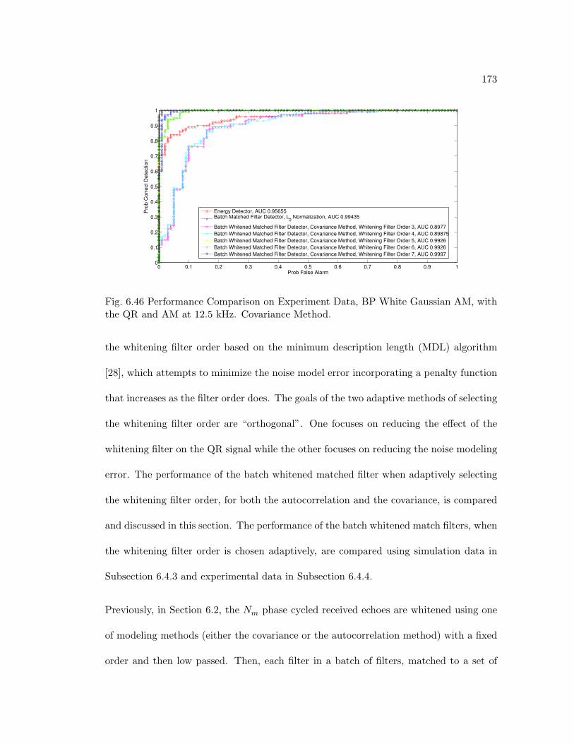
173
0 0.1 0.2 0.3 0.4 0.5 0.6 0.7 0.8 0.9 10
0.1
0.2
0.3
0.4
0.5
0.6
0.7
0.8
0.9
1
Pro
b C
orr
ect D
ete
ction
Prob False Alarm
Energy Detector, AUC 0.95655Batch Matched Filter Detector, L
2 Normalization, AUC 0.99435
Batch Whitened Matched Filter Detector, Covariance Method, Whitening Filter Order 3, AUC 0.8977
Batch Whitened Matched Filter Detector, Covariance Method, Whitening Filter Order 4, AUC 0.89875
Batch Whitened Matched Filter Detector, Covariance Method, Whitening Filter Order 5, AUC 0.9926
Batch Whitened Matched Filter Detector, Covariance Method, Whitening Filter Order 6, AUC 0.9926
Batch Whitened Matched Filter Detector, Covariance Method, Whitening Filter Order 7, AUC 0.9997
Fig. 6.46 Performance Comparison on Experiment Data, BP White Gaussian AM, withthe QR and AM at 12.5 kHz. Covariance Method.
the whitening filter order based on the minimum description length (MDL) algorithm
[28], which attempts to minimize the noise model error incorporating a penalty function
that increases as the filter order does. The goals of the two adaptive methods of selecting
the whitening filter order are “orthogonal”. One focuses on reducing the effect of the
whitening filter on the QR signal while the other focuses on reducing the noise modeling
error. The performance of the batch whitened matched filter when adaptively selecting
the whitening filter order, for both the autocorrelation and the covariance, is compared
and discussed in this section. The performance of the batch whitened match filters, when
the whitening filter order is chosen adaptively, are compared using simulation data in
Subsection 6.4.3 and experimental data in Subsection 6.4.4.
Previously, in Section 6.2, the Nm phase cycled received echoes are whitened using one
of modeling methods (either the covariance or the autocorrelation method) with a fixed
order and then low passed. Then, each filter in a batch of filters, matched to a set of
174
QR signals, is whitened and low passed using the same whitening and low pass filters
applied to the received signal. A decision on the presence of a QR signal is made based
on the maximum output of the batch of whitened match filters.
Unlike then, the gridding to match the QR signal parameters is performed pre-whitening
when designing the filters discussed in this section. The filters discussed in this section
use the approach in Section 5.2 to grid through the QR signal parameters and obtain
a periodic filter of Nm signals matched to the QR signal present. Since this part of
the process was discussed earlier it will not be repeated here. The next step would
be to whiten each of the Nm echoes of the filter (matched to the QR signal) using
a whitening filter (estimated by either the autocorrelation or covariance method) of
adaptively selected order. Selecting the whitening filter order is done according to one of
the methods introduced in this section. Each of these Nm whitened QR signals is then
low passed using the same 8-pole butterworth filter used in Section 6.2, denoted by M .
The Nm received echoes , xpci for i = 0, 1, . . . Nm− 1, are then whitened and low passed
using the same filters used to whiten and low pass the Nm echoes of the filter (matched
to the QR signal). Let the periodic filter matched to the QR signal, chosen as a result
of the process described in Section 5.2, be denoted as
h[k] =Nm−1∑i=0
sl,m,n[k − iNs], (6.13)
for k = 0, 1, . . . , Nm × Ns − 1, where sl,m,n[k] is a filter normalized in the l2 norm and
is matched to the lth, mth and nth frequency, phase and decaying parameter values
175
respectively. Each of these individual echoes is whitened using an estimated whitening
model (autocorrelation in Section 6.1.1 or covariance in Section 6.1.2) of order chosen
according to the least affect on the QR signal or the MDL algorithm. The following
two subsections describe how to adaptively choose the whitening filter order. These
methods can be applied whether the modeling method used is the autocorrelation or the
covariance method.
6.4.1 Whitening Filter Order that Least Effects the QR Signal
For a particular modeling method (auctorrelation or covariance method), the ith received
echo xpci is used to estimate a whitening model Wip of order p. This is repeated for a
number of model orders, Np, represented as a vector [plb, plb + 1, . . . , pub]. This process
leads to Np whitening matrices (Wi1, . . . ,Wi
Np). The whitening matrix that maximizes
maxjβijMWi
j sl,m,n[k]sTl,m,n
[k], (6.14)
is chosen, Wimax, where sl,m,n[k] is the normalized filter matched to the chosen QR
signal parameters, M is the 8-pole butterworth low pass filter, and βij is a constant that
normalizes the whitened low passed QR signal estimate MWij sl,m,n[k]. Maximizing the
above value ensures choosing the whitening filter order, between plb and pub that leads
to a whitening model that least deviates the whitened low passed QR signal from the
QR signal. This process is repeated for each of the Nm received signals resulting in Nm,
whitening matrices (W1max, . . . ,W1
max), where each can have a different model order.
176
The chosen whitening matrix for echo i, Wimax, along with the low pass filter M is
applied to the corresponding received echo i, as follows
xwi = βimaxMWi
maxxpci ,
where,
βimax =
∑Ns−1k=0
x2pci
[k]∑Ns−1k=0 (MWi
maxxpci [k])2.
Stringing these Nm signals in time leads to, xwmax
xwmax[k] = [xw0
[k], xw1[k −Ns], . . . .xwNm−1
[k − (Nm − 1)Ns], (6.15)
for k = 0, 1, . . . , Nm ×Ns − 1. Now that the received Nm echoes are whitened, the next
step is to whiten and low pass each of the Nm echoes of the periodic filter matched to
the QR signal as follows
hmax[k] = [sw0(l,m, n)[k], sw1
(l,m, n)[k −Ns], . . . , swNm−1(l,m, n)[k − (Nm− 1)Ns]
where,
swi(l,m, n)[k] =1
αwimax(l,m, n)
MWimaxe(−|−T/2+k∆|/Ta(n))cos(ωa(l)(−T/2 + k∆) + φa(m))
177
for k = 0, 1, . . . , Ns − 1. The value T is the length of the data acquisition window, Ns
is the number of discrete samples, ∆ = T/(Ns − 1) and αwimax(l,m, n) is a normalizing
constant.
The inner product of xwmax and hmax is then compared to threshold to determine the
presence of a QR signal. The following subsection describes the method of adaptively
choosing the whitening filter order according to the minimum description length (MDL)
algorithm [28].
6.4.2 Whitening Filter Order, Minimum Description Length Algorithm
This subsection explains how to use the minimum description length algorithm to adap-
tively determine the whitening filter order. For a particular modeling method (auctorre-
lation or covariance method), the ith received echo xpci is used to estimate a whitening
model Wip of order p. This is done for a number of model orders, Np, represented as a
vector [plb, plb+1, . . . , pub]. This process leads to Np whitening matrices (Wi1, . . . ,Wi
Np).
According to the minimum description algorithm, the whitening filter order p that min-
imizes the following function is chosen [28].
minp
[Ns log εp + (logNs)p] (6.16)
In the above equation, p represents the whitening filter order, Ns represents the number
of samples in an echo, and εp represents the minimized error shown in Equations (6.2)
and (6.4) when modeling using the autocorrelation and covariance methods respectively.
The idea behind the MDL algorithm is to increase the model order p until the modeling
178
error εp is minimized. However, since the error is a monotonically nonincreasing function
of the model order p, the MDL algorithm incorporates a penalty function that increases
with the model order p. This process is repeated with each of the Nm received signals
resulting in Nm, whitening matrices (W1max, . . . ,W1
max), where each can have a different
model order.
The rest of the procedure is identical to the procedure described in the above subsection
and therefore will not be repeated here. The following subsections use both simulation
and experimental data to compare the performance of the batch whitened matched filter,
where the order is selected adaptively.
6.4.3 Simulation Data
Figures (6.47)-(6.52) use simulation data to discuss the performance of the batch adap-
tive whitened matched filter. The whitening filters were estimated according to either the
autocorrelation or the covariance method, and the whitening filter order is chosen adap-
tively to either minimize the effect on the QR signal or according to the MDL algorithm.
The method gridded using the following values, ωlb = 0, ωub = 40000π, ω∆ = 100π,
φ∆ = .1, T ∗2 lb
= 300e−6, T ∗2 ub
= 900e−6 and T ∗2 ∆
= 100e−6. The above values lead to
Ndω = 401, Ndφ = 63 and NdT = 7 in each of the three dimensions, which corresponds to
Ndω ×Ndφ ×NdT = 176841 filters in the batch. After selecting the filter that resulted in
the maximum output, the adaptive whitening filters were applied. The filter order was
varied between plb = 3 and pub = 7 when adaptively selecting the whitening filter order.
179
The ROC plots in the figures compare the performance of the following four batch
adaptive whitened matched filters to the batch matched filter and the energy detector.
1. Batch Adaptive Whitened Matched Filter, whitened using autocorrelation method
with an adaptive order that least affects the QR signal.
2. Batch Adaptive Whitened Matched Filter, whitened using covariance method with
an adaptive order that least affects the QR signal.
3. Batch Adaptive Whitened Matched Filter, whitened using autocorrelation method
with an adaptive order selected according to the MDL algorithm.
4. Batch Adaptive Whitened Matched Filter, whitened using covariance method with
an adaptive order selected according to the MDL algorithm.
The ROC plots for the 2.5 kHz data set are shown in Figure (6.47). These results are
summarized in Table (6.11). The best batch adaptive whitened matched filter was the
one that used the autocorrelation method to model the noise with a filter order chosen
according to the MDL algorithm. This filter achieved an area under the curve (AUC)
of 0.875, which is lower but comparable to the performance of the batch matched filter
that achieved an AUC of 0.886. The other three batch adaptive whitened matched filters
achieved AUCs lower than that of the energy detector.
The best performing batch adaptive whitened matched filter when using the 5 kHz data
set, was the one that used the covariance method to model the noise with a filter of order
chosen according to the MDL algorithm. This is shown in Figure (6.48), where the ROC
curves of the different filters are compared. The results from this figure are summarized
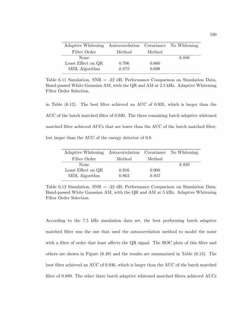
180
Adaptive Whitening Autocorrelation Covariance No WhiteningFilter Order Method Method
None 0.886Least Effect on QR 0.706 0.660
MDL Algorithm 0.875 0.698
Table 6.11 Simulation, SNR = -22 dB, Performance Comparison on Simulation Data,Band-passed White Gaussian AM, with the QR and AM at 2.5 kHz. Adaptive WhiteningFilter Order Selection.
in Table (6.12). The best filter achieved an AUC of 0.935, which is larger than the
AUC of the batch matched filter of 0.920. The three remaining batch adaptive whitened
matched filter achieved AUCs that are lower than the AUC of the batch matched filter,
but larger than the AUC of the energy detector of 0.8.
Adaptive Whitening Autocorrelation Covariance No WhiteningFilter Order Method Method
None 0.920Least Effect on QR 0.916 0.900
MDL Algorithm 0.863 0.935
Table 6.12 Simulation, SNR = -22 dB, Performance Comparison on Simulation Data,Band-passed White Gaussian AM, with the QR and AM at 5 kHz. Adaptive WhiteningFilter Order Selection.
According to the 7.5 kHz simulation data set, the best performing batch adaptive
matched filter was the one that used the autocorrelation method to model the noise
with a filter of order that least affects the QR signal. The ROC plots of this filter and
others are shown in Figure (6.49) and the results are summarized in Table (6.13). The
best filter achieved an AUC of 0.936, which is larger than the AUC of the batch matched
filter of 0.889. The other three batch adaptive whitened matched filters achieved AUCs
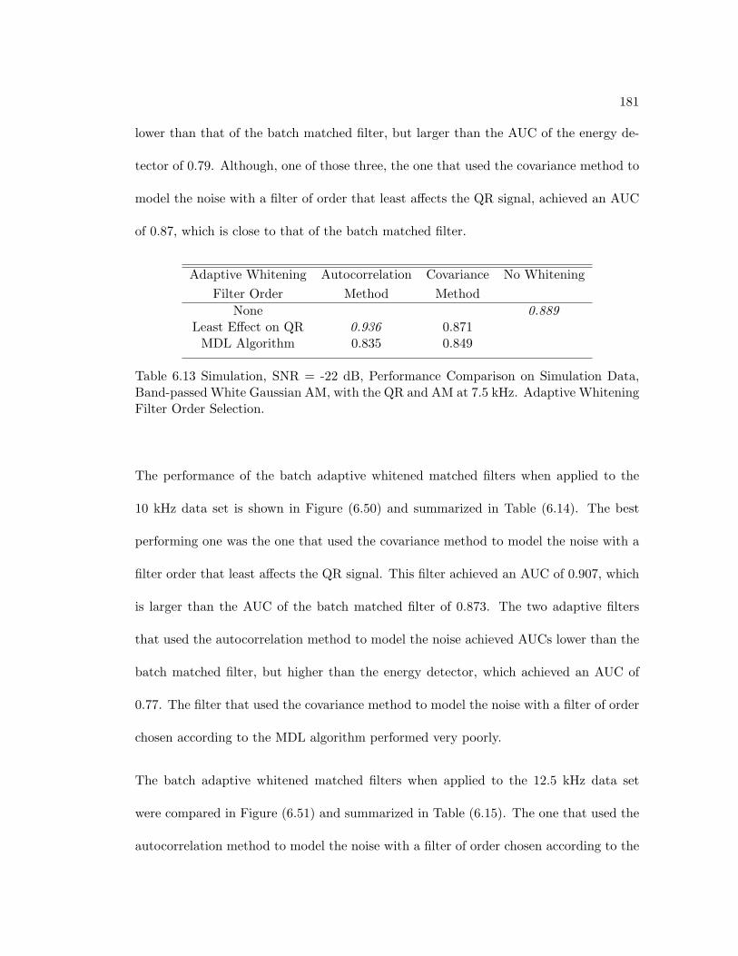
181
lower than that of the batch matched filter, but larger than the AUC of the energy de-
tector of 0.79. Although, one of those three, the one that used the covariance method to
model the noise with a filter of order that least affects the QR signal, achieved an AUC
of 0.87, which is close to that of the batch matched filter.
Adaptive Whitening Autocorrelation Covariance No WhiteningFilter Order Method Method
None 0.889Least Effect on QR 0.936 0.871
MDL Algorithm 0.835 0.849
Table 6.13 Simulation, SNR = -22 dB, Performance Comparison on Simulation Data,Band-passed White Gaussian AM, with the QR and AM at 7.5 kHz. Adaptive WhiteningFilter Order Selection.
The performance of the batch adaptive whitened matched filters when applied to the
10 kHz data set is shown in Figure (6.50) and summarized in Table (6.14). The best
performing one was the one that used the covariance method to model the noise with a
filter order that least affects the QR signal. This filter achieved an AUC of 0.907, which
is larger than the AUC of the batch matched filter of 0.873. The two adaptive filters
that used the autocorrelation method to model the noise achieved AUCs lower than the
batch matched filter, but higher than the energy detector, which achieved an AUC of
0.77. The filter that used the covariance method to model the noise with a filter of order
chosen according to the MDL algorithm performed very poorly.
The batch adaptive whitened matched filters when applied to the 12.5 kHz data set
were compared in Figure (6.51) and summarized in Table (6.15). The one that used the
autocorrelation method to model the noise with a filter of order chosen according to the
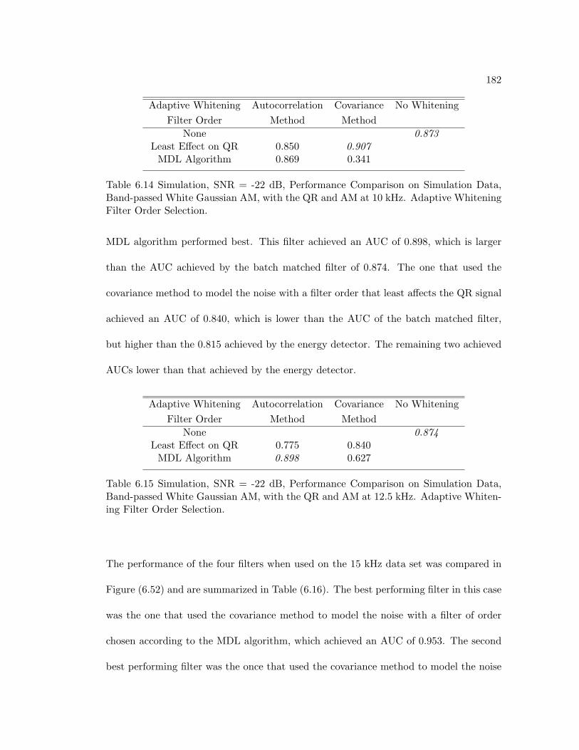
182
Adaptive Whitening Autocorrelation Covariance No WhiteningFilter Order Method Method
None 0.873Least Effect on QR 0.850 0.907
MDL Algorithm 0.869 0.341
Table 6.14 Simulation, SNR = -22 dB, Performance Comparison on Simulation Data,Band-passed White Gaussian AM, with the QR and AM at 10 kHz. Adaptive WhiteningFilter Order Selection.
MDL algorithm performed best. This filter achieved an AUC of 0.898, which is larger
than the AUC achieved by the batch matched filter of 0.874. The one that used the
covariance method to model the noise with a filter order that least affects the QR signal
achieved an AUC of 0.840, which is lower than the AUC of the batch matched filter,
but higher than the 0.815 achieved by the energy detector. The remaining two achieved
AUCs lower than that achieved by the energy detector.
Adaptive Whitening Autocorrelation Covariance No WhiteningFilter Order Method Method
None 0.874Least Effect on QR 0.775 0.840
MDL Algorithm 0.898 0.627
Table 6.15 Simulation, SNR = -22 dB, Performance Comparison on Simulation Data,Band-passed White Gaussian AM, with the QR and AM at 12.5 kHz. Adaptive Whiten-ing Filter Order Selection.
The performance of the four filters when used on the 15 kHz data set was compared in
Figure (6.52) and are summarized in Table (6.16). The best performing filter in this case
was the one that used the covariance method to model the noise with a filter of order
chosen according to the MDL algorithm, which achieved an AUC of 0.953. The second
best performing filter was the once that used the covariance method to model the noise
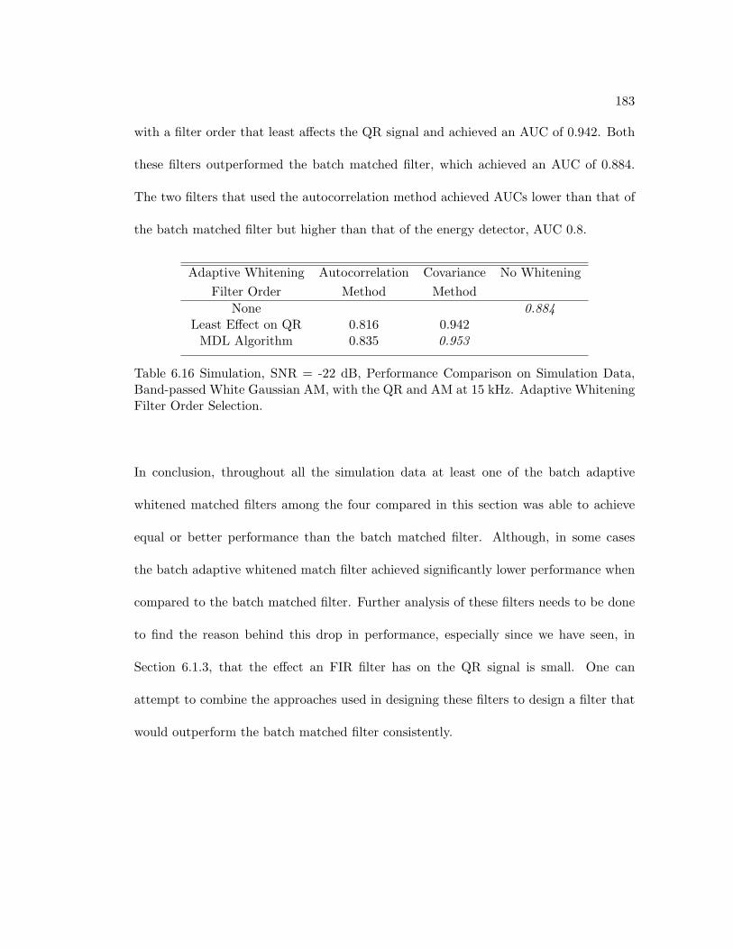
183
with a filter order that least affects the QR signal and achieved an AUC of 0.942. Both
these filters outperformed the batch matched filter, which achieved an AUC of 0.884.
The two filters that used the autocorrelation method achieved AUCs lower than that of
the batch matched filter but higher than that of the energy detector, AUC 0.8.
Adaptive Whitening Autocorrelation Covariance No WhiteningFilter Order Method Method
None 0.884Least Effect on QR 0.816 0.942
MDL Algorithm 0.835 0.953
Table 6.16 Simulation, SNR = -22 dB, Performance Comparison on Simulation Data,Band-passed White Gaussian AM, with the QR and AM at 15 kHz. Adaptive WhiteningFilter Order Selection.
In conclusion, throughout all the simulation data at least one of the batch adaptive
whitened matched filters among the four compared in this section was able to achieve
equal or better performance than the batch matched filter. Although, in some cases
the batch adaptive whitened match filter achieved significantly lower performance when
compared to the batch matched filter. Further analysis of these filters needs to be done
to find the reason behind this drop in performance, especially since we have seen, in
Section 6.1.3, that the effect an FIR filter has on the QR signal is small. One can
attempt to combine the approaches used in designing these filters to design a filter that
would outperform the batch matched filter consistently.
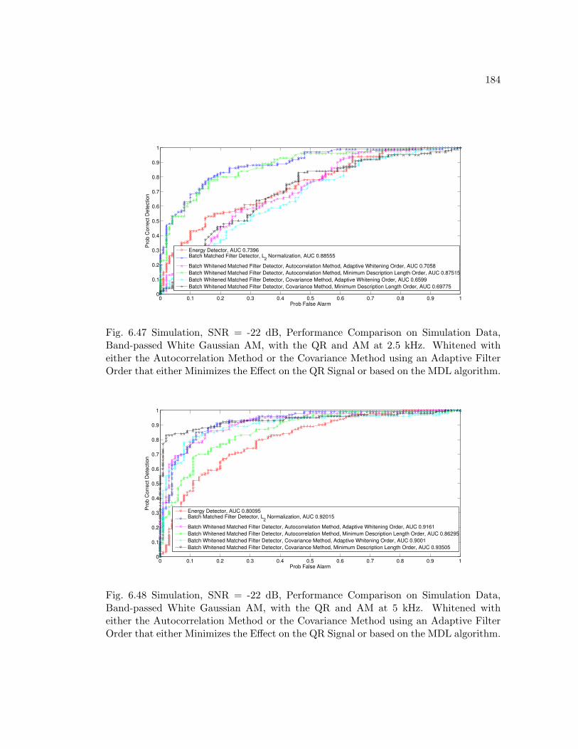
184
0 0.1 0.2 0.3 0.4 0.5 0.6 0.7 0.8 0.9 10
0.1
0.2
0.3
0.4
0.5
0.6
0.7
0.8
0.9
1P
rob C
orr
ect D
ete
ction
Prob False Alarm
Energy Detector, AUC 0.7396Batch Matched Filter Detector, L
2 Normalization, AUC 0.88555
Batch Whitened Matched Filter Detector, Autocorrelation Method, Adaptive Whitening Order, AUC 0.7058
Batch Whitened Matched Filter Detector, Autocorrelation Method, Minimum Description Length Order, AUC 0.87515
Batch Whitened Matched Filter Detector, Covariance Method, Adaptive Whitening Order, AUC 0.6599
Batch Whitened Matched Filter Detector, Covariance Method, Minimum Description Length Order, AUC 0.69775
Fig. 6.47 Simulation, SNR = -22 dB, Performance Comparison on Simulation Data,Band-passed White Gaussian AM, with the QR and AM at 2.5 kHz. Whitened witheither the Autocorrelation Method or the Covariance Method using an Adaptive FilterOrder that either Minimizes the Effect on the QR Signal or based on the MDL algorithm.
0 0.1 0.2 0.3 0.4 0.5 0.6 0.7 0.8 0.9 10
0.1
0.2
0.3
0.4
0.5
0.6
0.7
0.8
0.9
1
Pro
b C
orr
ect D
ete
ction
Prob False Alarm
Energy Detector, AUC 0.80095Batch Matched Filter Detector, L
2 Normalization, AUC 0.92015
Batch Whitened Matched Filter Detector, Autocorrelation Method, Adaptive Whitening Order, AUC 0.9161
Batch Whitened Matched Filter Detector, Autocorrelation Method, Minimum Description Length Order, AUC 0.86295
Batch Whitened Matched Filter Detector, Covariance Method, Adaptive Whitening Order, AUC 0.9001
Batch Whitened Matched Filter Detector, Covariance Method, Minimum Description Length Order, AUC 0.93505
Fig. 6.48 Simulation, SNR = -22 dB, Performance Comparison on Simulation Data,Band-passed White Gaussian AM, with the QR and AM at 5 kHz. Whitened witheither the Autocorrelation Method or the Covariance Method using an Adaptive FilterOrder that either Minimizes the Effect on the QR Signal or based on the MDL algorithm.
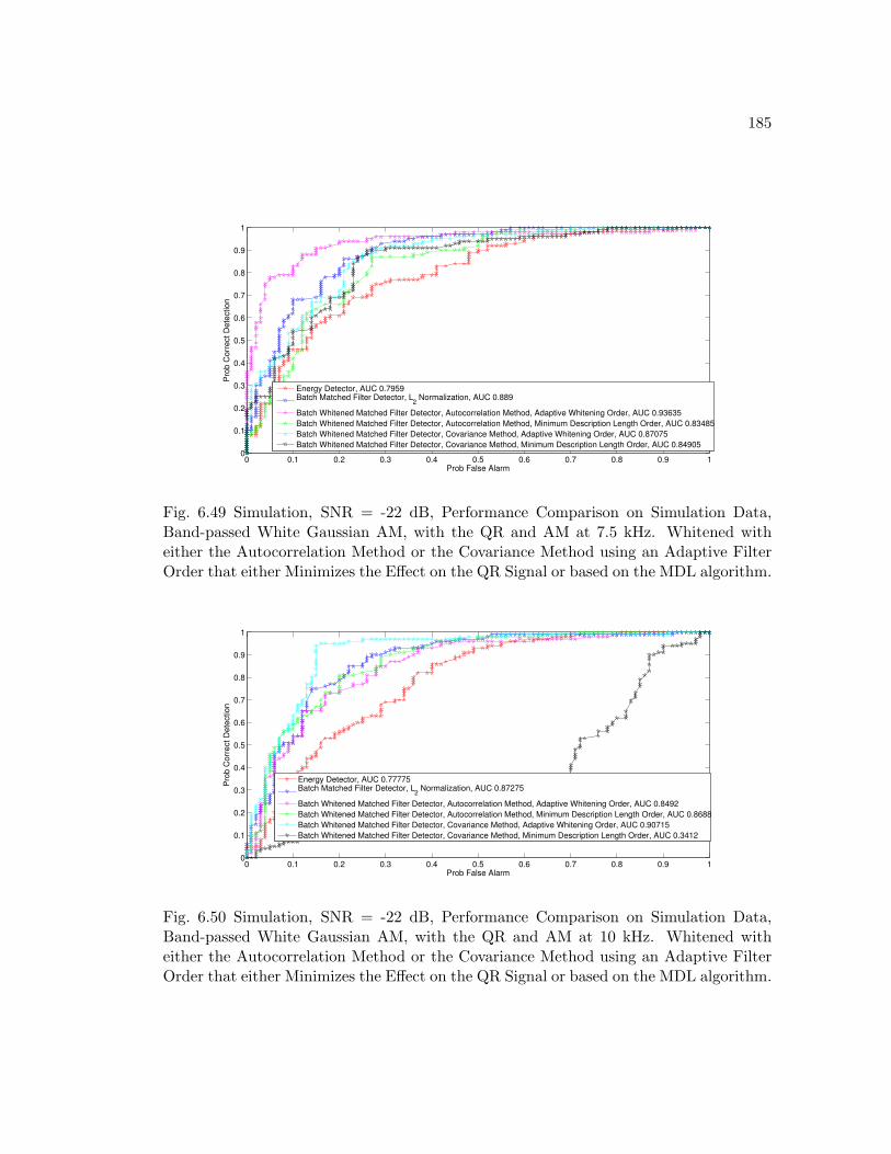
185
0 0.1 0.2 0.3 0.4 0.5 0.6 0.7 0.8 0.9 10
0.1
0.2
0.3
0.4
0.5
0.6
0.7
0.8
0.9
1P
rob C
orr
ect D
ete
ction
Prob False Alarm
Energy Detector, AUC 0.7959Batch Matched Filter Detector, L
2 Normalization, AUC 0.889
Batch Whitened Matched Filter Detector, Autocorrelation Method, Adaptive Whitening Order, AUC 0.93635
Batch Whitened Matched Filter Detector, Autocorrelation Method, Minimum Description Length Order, AUC 0.83485
Batch Whitened Matched Filter Detector, Covariance Method, Adaptive Whitening Order, AUC 0.87075
Batch Whitened Matched Filter Detector, Covariance Method, Minimum Description Length Order, AUC 0.84905
Fig. 6.49 Simulation, SNR = -22 dB, Performance Comparison on Simulation Data,Band-passed White Gaussian AM, with the QR and AM at 7.5 kHz. Whitened witheither the Autocorrelation Method or the Covariance Method using an Adaptive FilterOrder that either Minimizes the Effect on the QR Signal or based on the MDL algorithm.
0 0.1 0.2 0.3 0.4 0.5 0.6 0.7 0.8 0.9 10
0.1
0.2
0.3
0.4
0.5
0.6
0.7
0.8
0.9
1
Pro
b C
orr
ect D
ete
ction
Prob False Alarm
Energy Detector, AUC 0.77775Batch Matched Filter Detector, L
2 Normalization, AUC 0.87275
Batch Whitened Matched Filter Detector, Autocorrelation Method, Adaptive Whitening Order, AUC 0.8492
Batch Whitened Matched Filter Detector, Autocorrelation Method, Minimum Description Length Order, AUC 0.8688
Batch Whitened Matched Filter Detector, Covariance Method, Adaptive Whitening Order, AUC 0.90715
Batch Whitened Matched Filter Detector, Covariance Method, Minimum Description Length Order, AUC 0.3412
Fig. 6.50 Simulation, SNR = -22 dB, Performance Comparison on Simulation Data,Band-passed White Gaussian AM, with the QR and AM at 10 kHz. Whitened witheither the Autocorrelation Method or the Covariance Method using an Adaptive FilterOrder that either Minimizes the Effect on the QR Signal or based on the MDL algorithm.
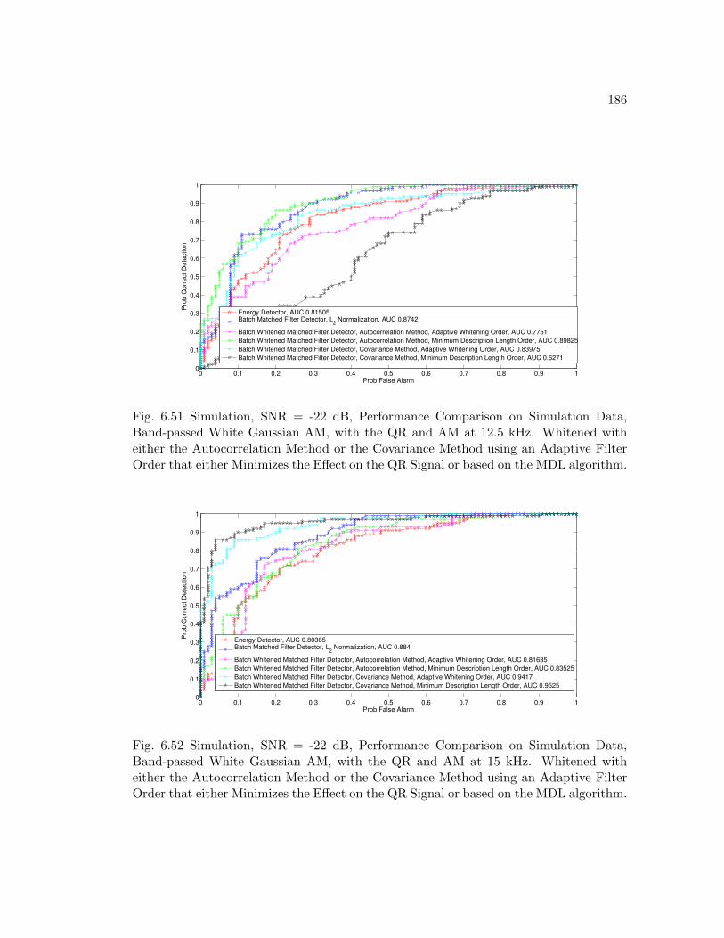
186
0 0.1 0.2 0.3 0.4 0.5 0.6 0.7 0.8 0.9 10
0.1
0.2
0.3
0.4
0.5
0.6
0.7
0.8
0.9
1P
rob C
orr
ect D
ete
ction
Prob False Alarm
Energy Detector, AUC 0.81505Batch Matched Filter Detector, L
2 Normalization, AUC 0.8742
Batch Whitened Matched Filter Detector, Autocorrelation Method, Adaptive Whitening Order, AUC 0.7751
Batch Whitened Matched Filter Detector, Autocorrelation Method, Minimum Description Length Order, AUC 0.89825
Batch Whitened Matched Filter Detector, Covariance Method, Adaptive Whitening Order, AUC 0.83975
Batch Whitened Matched Filter Detector, Covariance Method, Minimum Description Length Order, AUC 0.6271
Fig. 6.51 Simulation, SNR = -22 dB, Performance Comparison on Simulation Data,Band-passed White Gaussian AM, with the QR and AM at 12.5 kHz. Whitened witheither the Autocorrelation Method or the Covariance Method using an Adaptive FilterOrder that either Minimizes the Effect on the QR Signal or based on the MDL algorithm.
0 0.1 0.2 0.3 0.4 0.5 0.6 0.7 0.8 0.9 10
0.1
0.2
0.3
0.4
0.5
0.6
0.7
0.8
0.9
1
Pro
b C
orr
ect D
ete
ction
Prob False Alarm
Energy Detector, AUC 0.80365Batch Matched Filter Detector, L
2 Normalization, AUC 0.884
Batch Whitened Matched Filter Detector, Autocorrelation Method, Adaptive Whitening Order, AUC 0.81635
Batch Whitened Matched Filter Detector, Autocorrelation Method, Minimum Description Length Order, AUC 0.83525
Batch Whitened Matched Filter Detector, Covariance Method, Adaptive Whitening Order, AUC 0.9417
Batch Whitened Matched Filter Detector, Covariance Method, Minimum Description Length Order, AUC 0.9525
Fig. 6.52 Simulation, SNR = -22 dB, Performance Comparison on Simulation Data,Band-passed White Gaussian AM, with the QR and AM at 15 kHz. Whitened witheither the Autocorrelation Method or the Covariance Method using an Adaptive FilterOrder that either Minimizes the Effect on the QR Signal or based on the MDL algorithm.
187
6.4.4 Experimental Data
Figures (6.53)-(6.56) use experimental data to discuss the performance of the batch
adaptive whitened matched filter. The whitening filters were estimated according to
either the autocorrelation or the covariance method, and the whitening filter order is
chosen adaptively to either minimize the effect on the QR signal or according to the
MDL algorithm. The method gridded using the following values, ωlb = 0, ωub = 40000π,
ω∆ = 100π, φ∆ = .1, T ∗2 lb
= 300e − 6, T ∗2 ub
= 900e − 6 and T ∗2 ∆
= 100e − 6. The
above values lead to Ndω = 401, Ndφ = 63 and NdT = 7 in each of the three dimensions,
which corresponds to Ndω ×Ndφ ×NdT = 176841 filters in the batch. After selecting the
filter that resulted in the maximum output, the adaptive whitening filters were applied.
The range of filters to choose from is lower bounded by plb = 3 and upper bounded by
pub = 7, when adaptively selecting the whitening filter order.
The ROC plots in the figures below, compare the performance of the following four batch
adaptive whitened matched filters to the batch matched filter and the energy detector.
1. Batch Adaptive Whitened Matched Filter, whitened using autocorrelation method
with an adaptive order that least affects the QR signal.
2. Batch Adaptive Whitened Matched Filter, whitened using covariance method with
an adaptive order that least affects the QR signal.
3. Batch Adaptive Whitened Matched Filter, whitened using autocorrelation method
with an adaptive order selected according to the MDL algorithm.
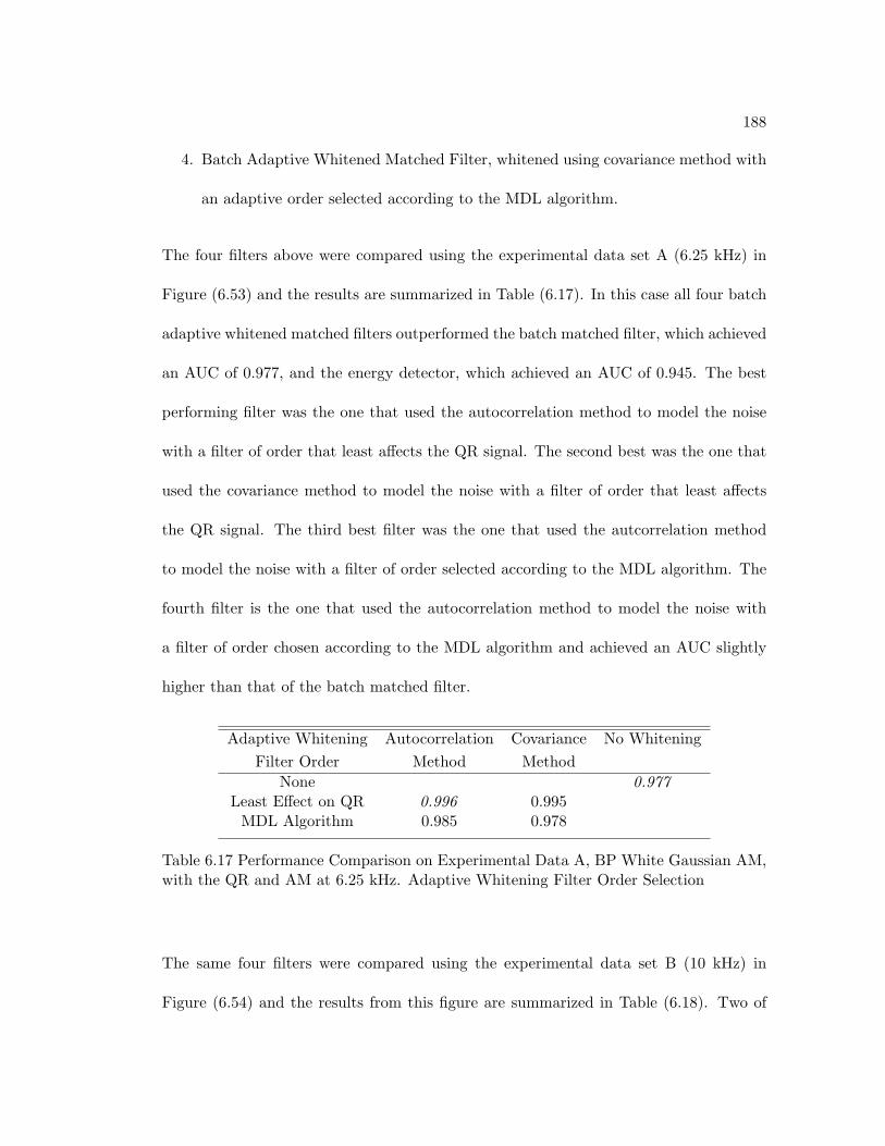
188
4. Batch Adaptive Whitened Matched Filter, whitened using covariance method with
an adaptive order selected according to the MDL algorithm.
The four filters above were compared using the experimental data set A (6.25 kHz) in
Figure (6.53) and the results are summarized in Table (6.17). In this case all four batch
adaptive whitened matched filters outperformed the batch matched filter, which achieved
an AUC of 0.977, and the energy detector, which achieved an AUC of 0.945. The best
performing filter was the one that used the autocorrelation method to model the noise
with a filter of order that least affects the QR signal. The second best was the one that
used the covariance method to model the noise with a filter of order that least affects
the QR signal. The third best filter was the one that used the autcorrelation method
to model the noise with a filter of order selected according to the MDL algorithm. The
fourth filter is the one that used the autocorrelation method to model the noise with
a filter of order chosen according to the MDL algorithm and achieved an AUC slightly
higher than that of the batch matched filter.
Adaptive Whitening Autocorrelation Covariance No WhiteningFilter Order Method Method
None 0.977Least Effect on QR 0.996 0.995
MDL Algorithm 0.985 0.978
Table 6.17 Performance Comparison on Experimental Data A, BP White Gaussian AM,with the QR and AM at 6.25 kHz. Adaptive Whitening Filter Order Selection
The same four filters were compared using the experimental data set B (10 kHz) in
Figure (6.54) and the results from this figure are summarized in Table (6.18). Two of
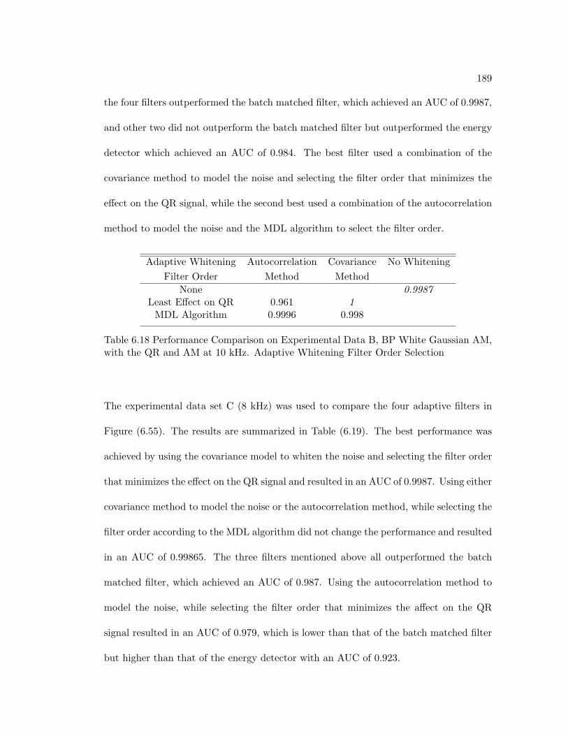
189
the four filters outperformed the batch matched filter, which achieved an AUC of 0.9987,
and other two did not outperform the batch matched filter but outperformed the energy
detector which achieved an AUC of 0.984. The best filter used a combination of the
covariance method to model the noise and selecting the filter order that minimizes the
effect on the QR signal, while the second best used a combination of the autocorrelation
method to model the noise and the MDL algorithm to select the filter order.
Adaptive Whitening Autocorrelation Covariance No WhiteningFilter Order Method Method
None 0.9987Least Effect on QR 0.961 1
MDL Algorithm 0.9996 0.998
Table 6.18 Performance Comparison on Experimental Data B, BP White Gaussian AM,with the QR and AM at 10 kHz. Adaptive Whitening Filter Order Selection
The experimental data set C (8 kHz) was used to compare the four adaptive filters in
Figure (6.55). The results are summarized in Table (6.19). The best performance was
achieved by using the covariance model to whiten the noise and selecting the filter order
that minimizes the effect on the QR signal and resulted in an AUC of 0.9987. Using either
covariance method to model the noise or the autocorrelation method, while selecting the
filter order according to the MDL algorithm did not change the performance and resulted
in an AUC of 0.99865. The three filters mentioned above all outperformed the batch
matched filter, which achieved an AUC of 0.987. Using the autocorrelation method to
model the noise, while selecting the filter order that minimizes the affect on the QR
signal resulted in an AUC of 0.979, which is lower than that of the batch matched filter
but higher than that of the energy detector with an AUC of 0.923.
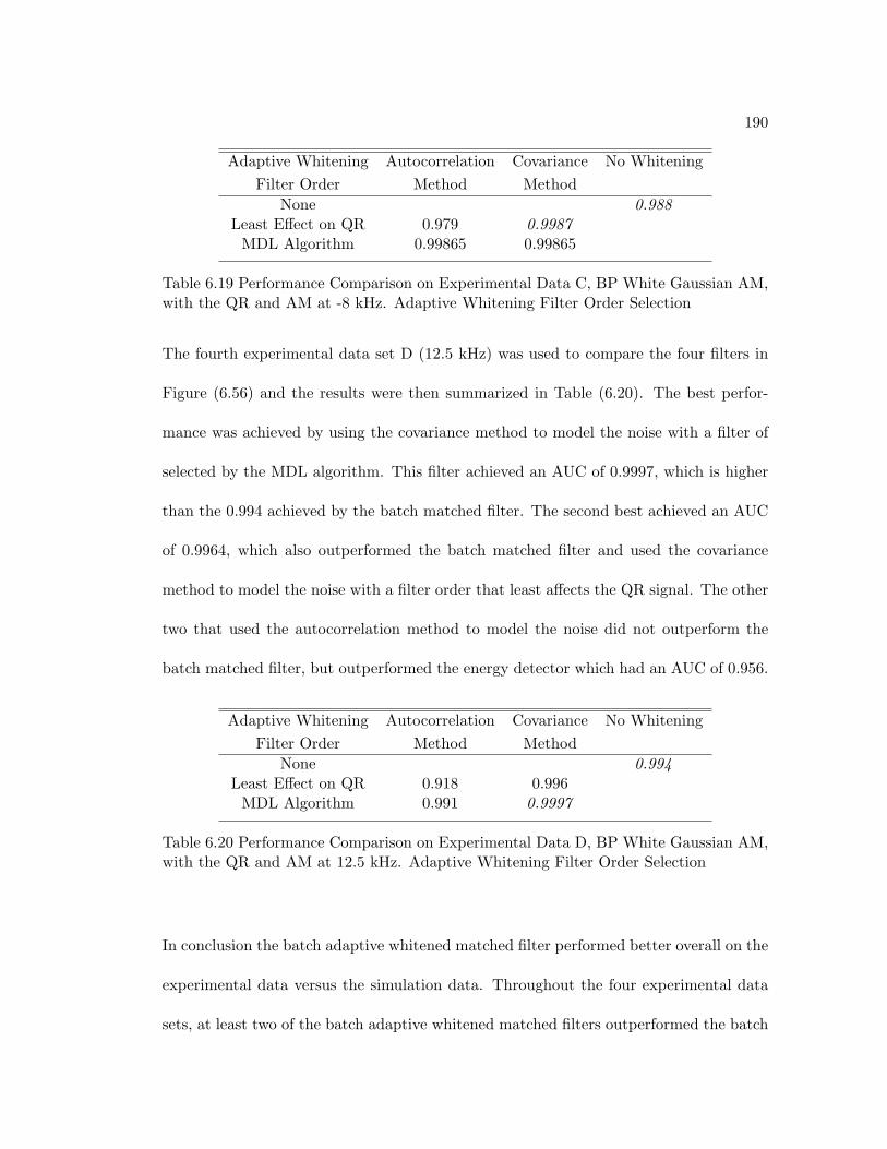
190
Adaptive Whitening Autocorrelation Covariance No WhiteningFilter Order Method Method
None 0.988Least Effect on QR 0.979 0.9987
MDL Algorithm 0.99865 0.99865
Table 6.19 Performance Comparison on Experimental Data C, BP White Gaussian AM,with the QR and AM at -8 kHz. Adaptive Whitening Filter Order Selection
The fourth experimental data set D (12.5 kHz) was used to compare the four filters in
Figure (6.56) and the results were then summarized in Table (6.20). The best perfor-
mance was achieved by using the covariance method to model the noise with a filter of
selected by the MDL algorithm. This filter achieved an AUC of 0.9997, which is higher
than the 0.994 achieved by the batch matched filter. The second best achieved an AUC
of 0.9964, which also outperformed the batch matched filter and used the covariance
method to model the noise with a filter order that least affects the QR signal. The other
two that used the autocorrelation method to model the noise did not outperform the
batch matched filter, but outperformed the energy detector which had an AUC of 0.956.
Adaptive Whitening Autocorrelation Covariance No WhiteningFilter Order Method Method
None 0.994Least Effect on QR 0.918 0.996
MDL Algorithm 0.991 0.9997
Table 6.20 Performance Comparison on Experimental Data D, BP White Gaussian AM,with the QR and AM at 12.5 kHz. Adaptive Whitening Filter Order Selection
In conclusion the batch adaptive whitened matched filter performed better overall on the
experimental data versus the simulation data. Throughout the four experimental data
sets, at least two of the batch adaptive whitened matched filters outperformed the batch
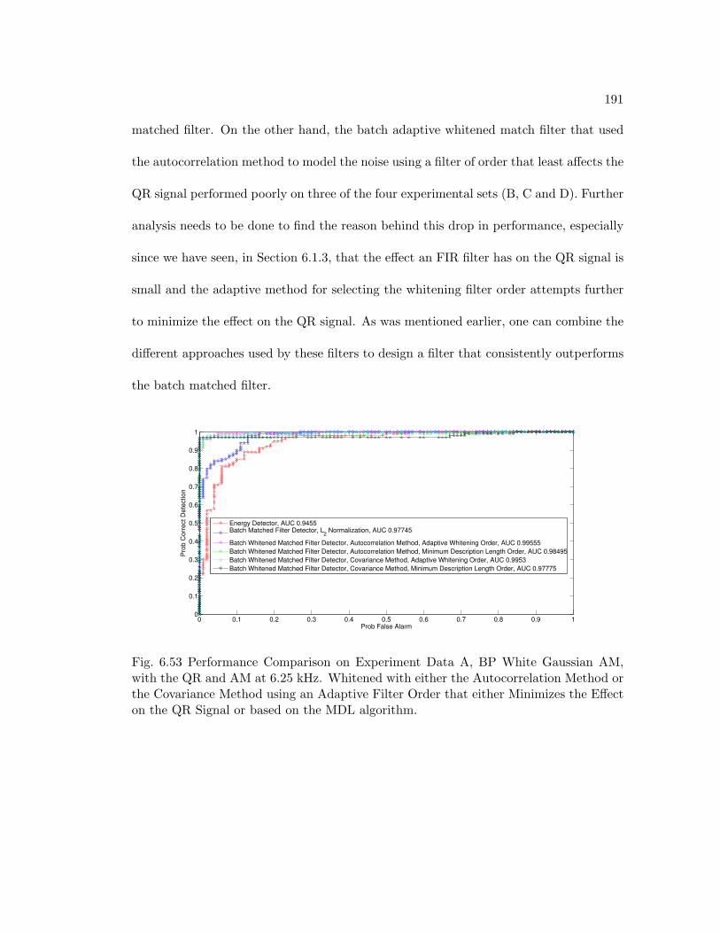
191
matched filter. On the other hand, the batch adaptive whitened match filter that used
the autocorrelation method to model the noise using a filter of order that least affects the
QR signal performed poorly on three of the four experimental sets (B, C and D). Further
analysis needs to be done to find the reason behind this drop in performance, especially
since we have seen, in Section 6.1.3, that the effect an FIR filter has on the QR signal is
small and the adaptive method for selecting the whitening filter order attempts further
to minimize the effect on the QR signal. As was mentioned earlier, one can combine the
different approaches used by these filters to design a filter that consistently outperforms
the batch matched filter.
0 0.1 0.2 0.3 0.4 0.5 0.6 0.7 0.8 0.9 10
0.1
0.2
0.3
0.4
0.5
0.6
0.7
0.8
0.9
1
Pro
b C
orr
ect D
ete
ction
Prob False Alarm
Energy Detector, AUC 0.9455Batch Matched Filter Detector, L
2 Normalization, AUC 0.97745
Batch Whitened Matched Filter Detector, Autocorrelation Method, Adaptive Whitening Order, AUC 0.99555
Batch Whitened Matched Filter Detector, Autocorrelation Method, Minimum Description Length Order, AUC 0.98495
Batch Whitened Matched Filter Detector, Covariance Method, Adaptive Whitening Order, AUC 0.9953
Batch Whitened Matched Filter Detector, Covariance Method, Minimum Description Length Order, AUC 0.97775
Fig. 6.53 Performance Comparison on Experiment Data A, BP White Gaussian AM,with the QR and AM at 6.25 kHz. Whitened with either the Autocorrelation Method orthe Covariance Method using an Adaptive Filter Order that either Minimizes the Effecton the QR Signal or based on the MDL algorithm.

192
0 0.1 0.2 0.3 0.4 0.5 0.6 0.7 0.8 0.9 10
0.1
0.2
0.3
0.4
0.5
0.6
0.7
0.8
0.9
1P
rob C
orr
ect D
ete
ction
Prob False Alarm
Energy Detector, AUC 0.98385Batch Matched Filter Detector, L
2 Normalization, AUC 0.9987
Batch Whitened Matched Filter Detector, Autocorrelation Method, Adaptive Whitening Order, AUC 0.9608
Batch Whitened Matched Filter Detector, Autocorrelation Method, Minimum Description Length Order, AUC 0.99955
Batch Whitened Matched Filter Detector, Covariance Method, Adaptive Whitening Order, AUC 1
Batch Whitened Matched Filter Detector, Covariance Method, Minimum Description Length Order, AUC 0.99775
Fig. 6.54 Performance Comparison on Experiment Data B, BP White Gaussian AM,with the QR and AM at 10 kHz. Whitened with either the Autocorrelation Method orthe Covariance Method using an Adaptive Filter Order that either Minimizes the Effecton the QR Signal or based on the MDL algorithm.
0 0.1 0.2 0.3 0.4 0.5 0.6 0.7 0.8 0.9 10
0.1
0.2
0.3
0.4
0.5
0.6
0.7
0.8
0.9
1
Pro
b C
orr
ect D
ete
ction
Prob False Alarm
Energy Detector, AUC 0.9231Batch Matched Filter Detector, L
2 Normalization, AUC 0.9878
Batch Whitened Matched Filter Detector, Autocorrelation Method, Adaptive Whitening Order, AUC 0.97925
Batch Whitened Matched Filter Detector, Autocorrelation Method, Minimum Description Length Order, AUC 0.99865
Batch Whitened Matched Filter Detector, Covariance Method, Adaptive Whitening Order, AUC 0.9987
Batch Whitened Matched Filter Detector, Covariance Method, Minimum Description Length Order, AUC 0.99865
Fig. 6.55 Performance Comparison on Experiment Data C, BP White Gaussian AM,with the QR and AM at -8 kHz. Whitened with either the Autocorrelation Method orthe Covariance Method using an Adaptive Filter Order that either Minimizes the Effecton the QR Signal or based on the MDL algorithm.
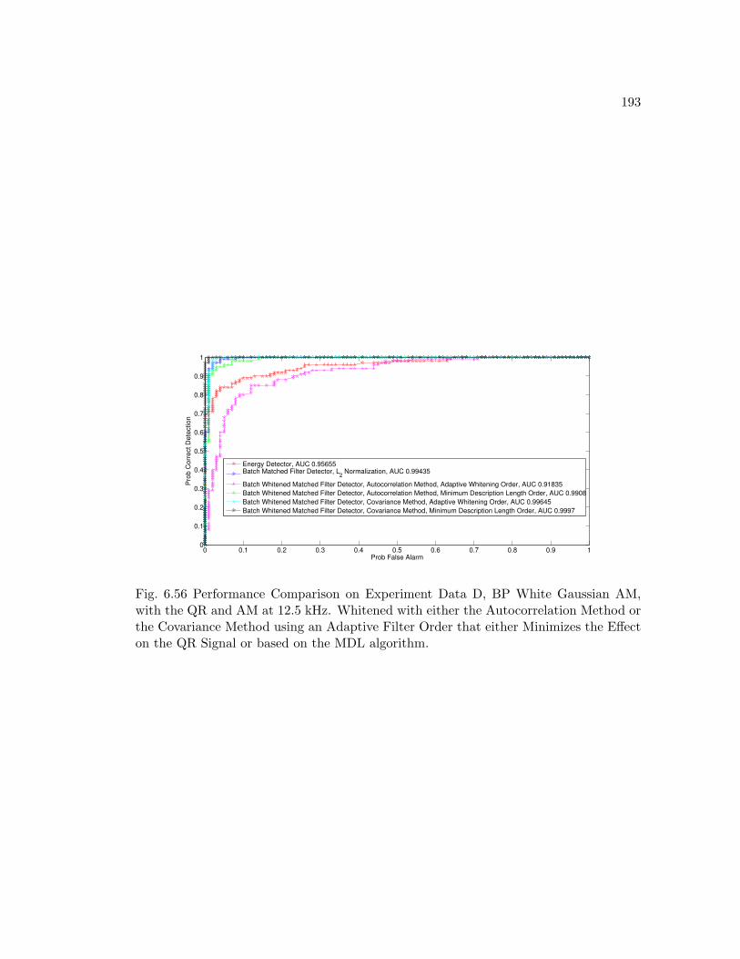
193
0 0.1 0.2 0.3 0.4 0.5 0.6 0.7 0.8 0.9 10
0.1
0.2
0.3
0.4
0.5
0.6
0.7
0.8
0.9
1
Pro
b C
orr
ect D
ete
ction
Prob False Alarm
Energy Detector, AUC 0.95655Batch Matched Filter Detector, L
2 Normalization, AUC 0.99435
Batch Whitened Matched Filter Detector, Autocorrelation Method, Adaptive Whitening Order, AUC 0.91835
Batch Whitened Matched Filter Detector, Autocorrelation Method, Minimum Description Length Order, AUC 0.9908
Batch Whitened Matched Filter Detector, Covariance Method, Adaptive Whitening Order, AUC 0.99645
Batch Whitened Matched Filter Detector, Covariance Method, Minimum Description Length Order, AUC 0.9997
Fig. 6.56 Performance Comparison on Experiment Data D, BP White Gaussian AM,with the QR and AM at 12.5 kHz. Whitened with either the Autocorrelation Method orthe Covariance Method using an Adaptive Filter Order that either Minimizes the Effecton the QR Signal or based on the MDL algorithm.
194
Chapter 7
Batch Whitened Robust Matched Filter
In Chapter 6, a gridding technique was combined with a whitening filter to design a
filter closely matched to both the QR signal and noise, when the QR signal and second
order statistics of the input noise are unknown. The performance of this filter drops,
when the parameters (frequency, phase and decaying value) of the QR signal present,
spc, fall in-between the values on the grid. For example, if the QR signal present, spc,
had a frequency of 12.1 kHz, a phase of .15 radians and a decaying parameter of 450e−6
and we grid in intervals of 200 Hz, .1 radians and 100e − 6 for frequency, phase and
decaying parameter respectively, none of the filters in the batch would exactly match
the QR signal present. This effect can be significantly reduced by using finer grids in
frequency, phase and decaying parameter, i.e. reducing each of the gridding intervals.
Another factor that can degrade performance is uncertainty in the general shape of the
QR signal. The ultimate goal of the robust matched filter approach in this chapter is
to address this uncertainty in the general shape of the QR signal, caused by narrow
bandwidth filters and receiver coils (HTS coil).
To address this uncertainty in the general shape of the signal, we propose designing a set
of filters, where each is robust to a set of QR signals and select the filter that results in
the maximum output. Each of the robust filters would be robust to a set of QR signals
with a fixed frequency, phase and decaying parameter but varies in the general shape.
195
Unfortunately, due to the lack of data with variances in the general shape of the QR
signal, we can not yet address the problem of robustness to these variances. Instead
this chapter will develop the tools to be used in designing the robust matched filters
and these methods will be applied to address robustness to variances in the QR signal
parameters and assume the general shape is known. These tools can later be applied
to design filters robust to uncertainties in the QR signal’s general shape for fixed signal
parameters.
Although uncertainties in the whitening filter (noise covariance matrix) are inevitable,
due to inaccuracies in the modeling estimates, this chapter will not address them but
will introduce the notion of filters that optimize performance for a pair of QR signal and
covariance matrix sets. The work will address the problem of designing a filter optimized
for a set of QR signals, while assuming our whitening approach proposed in Section 6.1
results in an exact match.
The chapter combines the gridding technique, the whitening filter, and the robust matched
filter introduced in Chapter 5, Section 6.1 and Section 7.5 respectively to form a batch
of robust whitened matched filters. As was mentioned earlier, the ultimate goal is to
achieve robustness to uncertainties in the QR signal’s shape but for now the uncertainty
will be restricted to the QR signal parameters that could be caused by unfine gridding.
Briefly the idea is to design a batch of whitened robust matched filters, where each filter
is whitened according to the noise present and is robust to a set of QR signals. Each
one of these filters is robust to a different set of QR signals, with frequency, phase and
196
decaying parameter that fall within intervals, which represents uncertainty in the signal’s
parameters. This batch of filters is used to determine the presence of a QR signal.
The following section introduces the idea of filters optimized for a pair of QR signal
and covariance matrix sets. This is followed by a section that introduces analytical
solutions for filters robust to two different pairs of QR signal and noise covariance sets,
one of which was derived by Verdu and Poor and the other was derived in this thesis. A
sampling approach to solving optimization problems, referred to as the scenario approach
is then introduced in Section 7.3. This approach to solving optimization problems will
be used in Section 7.4 in characterizing the set of QR signals using sampling, which is
a necessary step to use any of the analytical solutions introduced Section 7.2. Since
this chapter assumes that the whitening approach to estimating the covariance filter
leads to an exact value for the covariance matrix, the problem of characterizing a set
of covariance matrices is not addressed. The chapter moves on to directly using the
scenario approach to design an optimized matched filter for a set of QR signal samples
by solving an optimization problem, without having to first characterize the set of QR
signals. This is the most feasible approach for designing filters robust to a set of the
QR signals. This approach is combined with the gridding technique and whitening filter
introduced in Chapter 5 and Section 6.1 to create a batch robust whitened matched filter
in Section 7.6. The performance of this filter in the presence of noise is discussed using
simulation data in the last section of the chapter.
197
7.1 Robust Matched Filter
In the case when the signal and noise are not exactly known but are known to fall
within a particular uncertainty set, since no filter will be optimum for every member
of the uncertainty set, it is of interest to design a robust filter. The robust filter would
guarantee a certain level of performance for the set of possible input signal and noise
pairs, independently of which member of the uncertainty set is actually present.
There are several different approaches to designing this robust filter; one well established
approach is the minimax strategy, used in this thesis. The goal here is to optimize the
performance of the filter for the worst-case signal-noise pair. There are several studies
on the minimax strategy to robust matched filtering [16; 62; 61], but this section will
focus on robust finite-length discrete time matched filters.
Consider the following problem formulation [65]: Let H be a Hilbert space with inner
product < ·, · > and P a set of bounded, linear, self-adjoint, positive operators mapping
H to itself. Now, if the input signal and noise quantities are known only to belong to
some uncertainty classes S ⊂ H, N ⊂ P , then a possible optimal filter design strategy is
to choose the one that exhibits the best performance for the worst-case signal and noise
pair in Q = S×N (the cartesian product of the uncertainty sets) i.e., to choose hR such
that
hR = arg maxh∈H
inf(s,Σ)∈S×N
ρ(h; s,Σ) (7.1)
198
Another way of explaining Equation (7.1), is that of a least favorable signal and noise
pair, (sL,ΣL), defined by the relationship
(sL,ΣL) = arg min(s,Σ)∈S×N
ρ(h∗(s,Σ); s,Σ), (7.2)
where, h∗(s,Σ), is the optimal matched filter for the signal and noise pair (s,Σ). So
(sL,ΣL) is the pair in the uncertainty class with minimum optimal signal-to-noise ratio.
This design problem can be thought of as a game (H,S×N, ρ), where the designer tries
to maximize the function ρ by selecting a filter from the set H and the opponent (nature)
tries to minimize it by choosing a signal and noise pair from S×N . The following shows
that the filter, hL, optimal to the signal noise pair (sL,ΣL), referred to as a saddle point,
is in fact the minimax robust filter.
If a saddle point exists for this game, which means if there is a point [hL, (sL,ΣL)] that
satisfies
ρ(h; sL,ΣL) ≤ ρ(hL; sL,ΣL) ≤ ρ(hL; s,Σ) (7.3)
for all h ∈ H, s ∈ S, and Σ ∈ N , then hL has its worst performance at (sL,ΣL), and any
other filter has worst behavior at (sL,ΣL), which implies that hL is the minimax robust
filter. Furthermore, from the definition of h∗(s,Σ), we have
ρ(hL; s,Σ) ≤ ρ(h∗(s,Σ); s,Σ) (7.4)
which, together with Equation (7.3) implies that (sL,ΣL) is a least favorable pair.
199
The existence and characterization of a saddle point for the robust matched filtering
problem in (7.1) can be straightforwardly derived from (4.8) and (7.3) and are summa-
rized in the following lemma. A proof of this lemma can be found in [65].
Lemma 7.1. (hL, (sL,ΣL)) is a saddle point for (H,S ×N, ρ) if and only if
1. ΣLhL = sL
2. | < sL, hL > | ≤ | < s, hL > | ∀s ∈ S
3. 0 ≤ < hL, (ΣL − Σ)hL > ∀Σ ∈ N
Solving the equations of Lemma (7.1) would result in a saddle point of (H,S×N, ρ). The
above lemma is an important result and can be used to derive analytical filter solutions
for specific uncertainty models. Another important result presented in [65] is Theorem
(7.2), which requires defining the term regular pair. The following theorem, [65] defines
the term regular pair.
Theorem 7.1. Denote hL = h∗(sL,ΣL), Q = S × N (the cartesian product of the
uncertainty sets) and define the functional f : H ×H × P × P × [0, 1] → C where C is
the complex scalar field of H by
f(a, b,A,B, α) ≡< b−Bh∗(a,A),h∗(a− α(a− b),A− α(A−B)) > (7.5)
200
If for every (s,Σ) ∈ Q such that (sα,Σα) = (1−α)(sL,ΣL)+α(s,Σ) ∈ Q for all α ∈ [0, 1],
we have that f(sL, s,ΣL,Σ, .) is right continuos at the origin, then (hL, (sL,ΣL)) is a
regular pair for (H,Q, ρ).
The regularity condition can also be seen as requiring the difference of performance
achieved by the optimal filter, hα, at (sα,Σα) (a point close to (sL,ΣL)) and by hL at
(sα,Σα), divided by α, to go to zero when α goes to zero. This condition is used in
the following theorem, which simplifies the robust matched filtering problem for the case
when the uncertainty set is convex.
Theorem 7.2. Suppose that Q = S ×N , the cartesian product of the uncertainty sets,
is a convex set and that ρ(h; , ) is convex on Q for every h ∈ H.
Then if the pair of filter and signal/noise (hL; sL,ΣL) is a regular pair of (H,S ×N, ρ),
the following statements are equivalent,
1. (sL,ΣL) is a least favorable operating point of (H,S ×N, ρ)
2. (hL; sL,ΣL) is a saddle point point solution of (H,S ×N, ρ)
It has been shown in [41] that the signal to noise ratio defined in (4.8) is convex in (s,Σ)
for every h ∈ H. Theorem 7.1 stated that under a mild continuity condition on the
behavior of the matched filter around a given operating point (sL,ΣL), this point and
its optimal filter form a regular pair. Furthermore, it has been proved in [65], that the
invertibility of ΣL is a sufficient condition for the continuity condition to hold. Therefore,
if the uncertainty class Q is convex and the regularity condition holds (i.e. the conditions
of Theorem 7.2 are satisfied) then the problem of finding a saddle point (minimax robust
201
filter), whenever one exists, is reduced to that of finding a least favorable pair of signal
and noise. This need not be easier than the original problem of finding a minimax robust
matched filter. However, the existence of an explicit expression for ρ∗(.) (Equation 4.11)
reduces the search for least favorable operating points to a convex minimization problem,
at which point, a directional derivative approach can be used.
The results of Lemma 7.1 and Theorems 7.1 and 7.2 were used by Verdu and Poor in [66]
to derive analytical solutions for several types of uncertainty sets. As examples, one of
these cases is presented in the next section as along with the solution to another signal
and noise pair (derived in this thesis using the results of Lemma 7.1).
7.2 Analytical Solutions For Robust Matched Filters Over Particular
Uncertainty Sets
This section provides analytic solutions to the matched filter robust to specific signal and
noise uncertainty sets. Considering the time-domain formulation, where H = <k, P =
{Σ ∈ <k×k,Σ > 0}, s = [s[0], . . . , s[k−1]]T and h = [h0, . . . , h[k−1]]T , h[i] = h[k−1− i],
and s[i] and h[i] are the values of the signal and of the filter response, respectively, at
the ith sample. The following subsection presents the analytic solution for a filter robust
to a spherical signal set and matrix norm bounded noise set pair, derived by Verdu and
Poor [66]. This is followed by a another subsection that derives the analytical solution
of the filter robust to an elliptical signal set and matrix norm bounded noise set.
202
7.2.1 Spherical Signal Set and Noise Uncertainty Bounded by a Matrix
Norm
If the signal uncertainty is modeled by a bound on the mean-square distortion S1 as
follows,
S1 = {s ∈ <k,k−1∑i=0
|s[i]− s0[i]|2 ≤ 42} (7.6)
and the noise uncertainty is modeled by a bound on some matrix norm of the deviation
from a nominal, N1
N1 = {Σ ∈ <k×k, ||Σ− Σ0|| ≤ ε,Σ > 0} (7.7)
where the norm in (7.7) is a unit matrix norm (if ||I|| = 1, then ||.|| is a unit matrix
norm). It has been proven by Verdu and Poor in [66] that the optimal robust filter is
of the form
hL = (Σ0 + (ε+ σs2)I)−1s0 (7.8)
where σs2 is defined by σs
2||hL||2 = 4. The corresponding least favorable signal and
noise pair has been shown to have the following form,
sL = s0 − σs2hL (7.9)
ΣL = Σ0 + εI (7.10)
203
Verdu and Poor in [66] have also considered other signal uncertainty sets, where the
distortion measure is bounded in the l1 and l∞ norms, and other noise covariance un-
certainty sets, where the perturbations from the nominal covariance matrix are bounded
in the l2 norm. Unfortunately in [66] the case when the uncertainty in the QR signal
is unevenly spaced is not discussed. Uneven weights can be placed on the uncertainty
of the QR signal if an ellipse is used to to describe the uncertainty set. Fortunately
enough, Lemma 7.1 can be used to derive analytical solutions for particular signal and
noise uncertainty sets.
7.2.2 Elliptic Signal Set and Noise Uncertainty Bounded by the Frobenius
Matrix Norm or the 2-Norm
We used the lemma to derive an analytical solution for a signal uncertainty set bounded
by an ellipse and a noise uncertainty set modeled by a bound in either the Frobenius
norm or the l2 norm (the results is unchanged for both these norms). If the signal
uncertainty is modeled by an ellipse S2 as follows,
S2 = {s ∈ <k, (s− s0)TW (s− s0) ≤ 42} (7.11)
which is a convex set. The noise uncertainty is modeled by a bound on the deviation
from the nominal. This bound can be in any matrix norm that satisfies the property
||xxT || = xTx, where x ∈ <k×1. Both the Frobenius and the 2-norm satisfy this property,
so without loss of generality we will define the noise uncertainty set in the l2 norm, N2,
as follows,
204
N2 = {Σ ∈ <k×k, ||Σ− Σ0||2 ≤ ε,Σ > 0}. (7.12)
The minimax solution for the uncertainty sets S2 and N2, can characterized by the
following result.
Proposition 1. (hL, (sL,ΣL)) is a saddle point for (H,S2 ×N2, ρ) if and only if
sL = s0 − λW−1hL and λ = 4||W−1/2hL||2
with
ΣL = Σ0 + σn2hLhL
T and σn2||hL||22 = ε
and
ΣLhL = sL
Proof: Using the above proposition we can solve for the robust minimax filter hL as
follows
205
ΣLhL = sL
(Σ0 + σn2hLhL
T )hL = s0 − λW−1hL
Σ0hL + σn2||hL||
22hL + λW−1hL = s0
Σ0hL + εhL + λW−1hL = s0
(Σ0 + ε+ λW−1)hL = s0
hL = (Σ0 + ε+ λW−1)−1s0
and
λ||W−1/2hL|| = 4
λ||(Σ0W1/2 + εW 1/2 + λW−1/2)−1s0|| = 4
where the function of λ, f(λ), to the left of the equality sign has a solution, since f(0) = 0
and the limλ→∞ f(λ) = ||W 1/2s0||. Next, we show that Lemma 7.1.2 is true, which is
equivalent to 〈s− sL, hL〉 ≥ 0, ∀s ∈ S2 since S2 is a convex set.
206
< s− sL, hL > = < W 1/2(s− sL),W−1/2hL >
= < W 1/2((s− s0)− (sL − s0)),W−1/2hL >
= < W 1/2(s− s0),W−1/2hL > − < W 1/2(sL − s0),W−1/2hL >
= < W 1/2(s− s0),W−1/2hL > +λ < W−1/2hL,W−1/2hL >
≥ −| < W 1/2(s− s0),W−1/2hL > |+4||W−1/2hL||
≥ −||W 1/2(s− s0)||||W−1/2hL||+4||W−1/2hL|| ≥ 0
Lastly, we show that Lemma 7.1.3 is true as follows.
< hL, (ΣL − Σ)hL > = < hL, (Σ0 + σn2hLhL
T − Σ)hL >
= σn2(hL
ThL)2+ < hL, (Σ0 − Σ)hL >
= ε||hL||22+ < hL, (Σ0 − Σ)hL >
207
where
< hL, (Σ0 − Σ)hL > ≥ −| < hL, (Σ0 − Σ)hL > |
≥ −||hL||||(Σ0 − Σ)hL||
≥ −||hL||2||(Σ0 − Σ)hL||
therefore,
< hL, (ΣL − Σ)hL > ≥ ε||hL||22− ||hL||
2||(Σ0 − Σ)hL||
≥ ||hL||22(ε− ||Σ0 − Σ||)
≥ 0.
To utilize the analytical solutions for the robust matched filters derived in the section
above, a characterization of the set of QR signals one would like to be robust to is needed.
This problem is addressed in Section 7.4, though before that the scenario approach to
probabilistic robust design is introduced in the next section. This approach is used to
characterize signal sets through sampling in Section 7.4, and this same approach can be
used to characterize an ellipse or any other shaped signal set. The problem of character-
izing noise uncertainty sets will not be discussed, since throughout the remainder of this
chapter we will be assuming that our whitening approach to estimating the covariance
matrix leads to accurate values. The scenario approach to robust design is also used in
208
solving for matched filters robust, maximizes SNR, to a set of QR signals where the pa-
rameters vary within lower and upper bounds in the presence of thermal noise in Section
7.5. The following section uses a sampling approach to characterize a set of signals.
7.3 The Scenario Approach
This section introduces a probabilistic approach to robustness referred to as the scenario
approach. The scenario approach can be used to modify a robust optimization problem
with an infinite number of constraints into a one with a finite number of constraints.
If we consider our optimization problem to be
minimize cT [h; γ]
subject to J(s, h) ≤ γ ∀s ∈ S.
where, S ⊂ <k, h ∈ H ⊂ <k, J(s, h) : S ×H → < is convex in h, for all s ∈ S and H
is a convex and closed subset of <k. Then an alternative approach to solving the above
difficult problem is to redefine it using the scenario approach [43], as follows. If s is a
random variable variable with an assigned probability distribution over S, then s(1,...,N)
denotes a multi-sample s1, . . . , sN of independent samples of S extracted according to
some probability distribution. These samples, s(1,...,N), represent the randomly selected
scenarios and used in defining the following scenario design problem [43].
minimize cT [h; γ]
subject to J(si, h) ≤ γ i = 1, . . . , N.
209
This is a standard convex program, with a finite number of constraints, and as such
it is usually computationally tractable. If the number of samples N is properly chosen
then the optimal solution returned by the scenario approach is with high probability
robust to the original design problem. Tempo [43], discusses the relationship between
N and the probability of robustness of the original problem but since in reality the
computational solver used is what places the limitations on N , this relationship is not
discussed here. This approach is used in the following section to characterize signal sets
by solving robust design problems. The scenario approach is also used in Section 7.5 to
design robust matched filters, without characterizing the uncertainty set, by solving an
optimization problem.
7.4 Characterizing a Set of QR Signals Through Sampling
Since this chapter will address robustness to uncertainties in the QR signal parameters
and not uncertainties in the general shape, examples of characterizing QR sets with
parametric uncertainty are presented in this section. This approach to characterizing
sets can be applied to characterizing any QR signal set, such as a set with uncertainty
in the general shape of the signal. The characterization of signal sets is required to use
any of the results in the section above.
The section uses a sampling approach to characterize the set of QR signals, S,
s[k] = Ae(−|−T/2+k∆|/T2∗) cos (ωbb(−T/2 + k∆) + φbb).
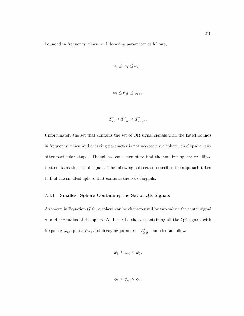
210
bounded in frequency, phase and decaying parameter as follows,
ωi ≤ ωbb ≤ ωi+1
φi ≤ φbb ≤ φi+1
T ∗2 i≤ T ∗
2 bb≤ T ∗
2 i+1.
Unfortunately the set that contains the set of QR signal signals with the listed bounds
in frequency, phase and decaying parameter is not necessarily a sphere, an ellipse or any
other particular shape. Though we can attempt to find the smallest sphere or ellipse
that contains this set of signals. The following subsection describes the approach taken
to find the smallest sphere that contains the set of signals.
7.4.1 Smallest Sphere Containing the Set of QR Signals
As shown in Equation (7.6), a sphere can be characterized by two values the center signal
s0 and the radius of the sphere ∆. Let S be the set containing all the QR signals with
frequency ωbb, phase φbb, and decaying parameter T ∗2 bb
, bounded as follows
ω1 ≤ ωbb ≤ ω2,
φ1 ≤ φbb ≤ φ2,
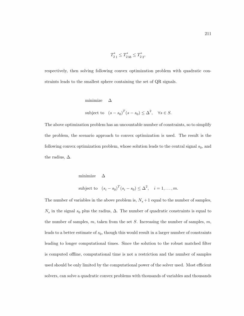
211
T ∗2 1≤ T ∗
2 bb≤ T ∗
2 2,
respectively, then solving following convex optimization problem with quadratic con-
straints leads to the smallest sphere containing the set of QR signals.
minimize ∆
subject to (s− s0)T (s− s0) ≤ ∆2, ∀s ∈ S.
The above optimization problem has an uncountable number of constraints, so to simplify
the problem, the scenario approach to convex optimization is used. The result is the
following convex optimization problem, whose solution leads to the central signal s0, and
the radius, ∆.
minimize ∆
subject to (si − s0)T (si − s0) ≤ ∆2, i = 1, . . . ,m.
The number of variables in the above problem is, Ns+1 equal to the number of samples,
Ns in the signal s0 plus the radius, ∆. The number of quadratic constraints is equal to
the number of samples, m, taken from the set S. Increasing the number of samples, m,
leads to a better estimate of s0, though this would result in a larger number of constraints
leading to longer computational times. Since the solution to the robust matched filter
is computed offline, computational time is not a restriction and the number of samples
used should be only limited by the computational power of the solver used. Most efficient
solvers, can solve a quadratic convex problems with thousands of variables and thousands
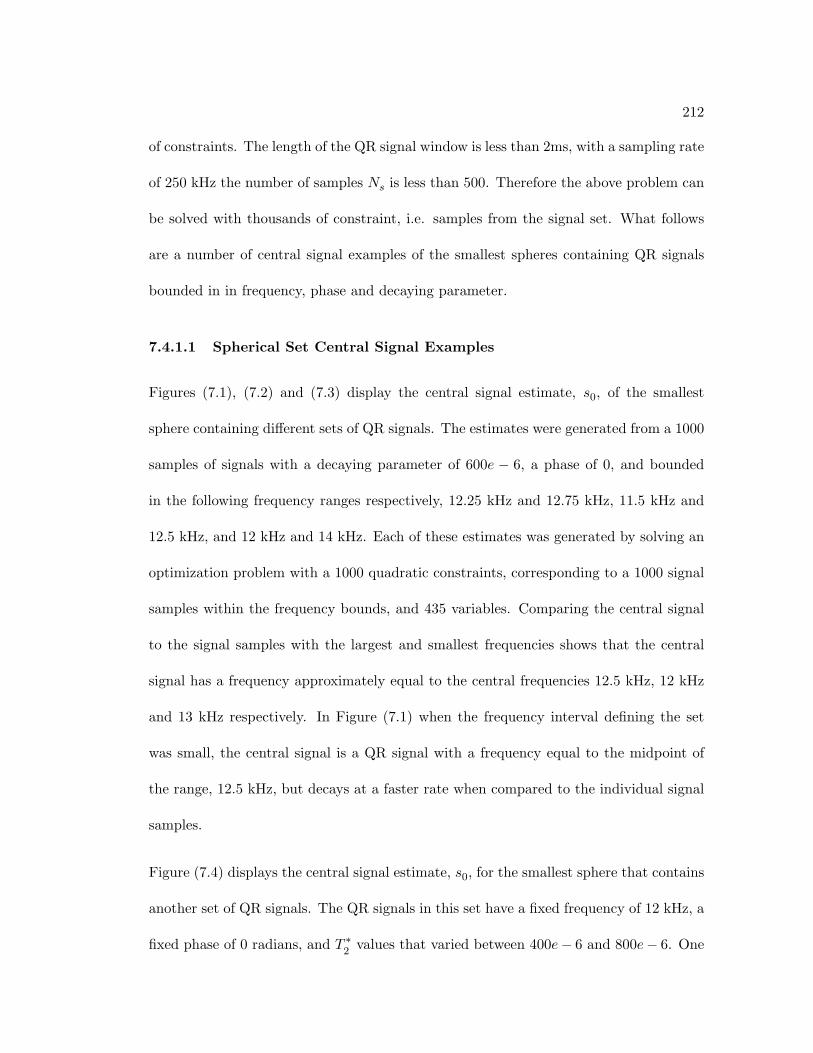
212
of constraints. The length of the QR signal window is less than 2ms, with a sampling rate
of 250 kHz the number of samples Ns is less than 500. Therefore the above problem can
be solved with thousands of constraint, i.e. samples from the signal set. What follows
are a number of central signal examples of the smallest spheres containing QR signals
bounded in in frequency, phase and decaying parameter.
7.4.1.1 Spherical Set Central Signal Examples
Figures (7.1), (7.2) and (7.3) display the central signal estimate, s0, of the smallest
sphere containing different sets of QR signals. The estimates were generated from a 1000
samples of signals with a decaying parameter of 600e − 6, a phase of 0, and bounded
in the following frequency ranges respectively, 12.25 kHz and 12.75 kHz, 11.5 kHz and
12.5 kHz, and 12 kHz and 14 kHz. Each of these estimates was generated by solving an
optimization problem with a 1000 quadratic constraints, corresponding to a 1000 signal
samples within the frequency bounds, and 435 variables. Comparing the central signal
to the signal samples with the largest and smallest frequencies shows that the central
signal has a frequency approximately equal to the central frequencies 12.5 kHz, 12 kHz
and 13 kHz respectively. In Figure (7.1) when the frequency interval defining the set
was small, the central signal is a QR signal with a frequency equal to the midpoint of
the range, 12.5 kHz, but decays at a faster rate when compared to the individual signal
samples.
Figure (7.4) displays the central signal estimate, s0, for the smallest sphere that contains
another set of QR signals. The QR signals in this set have a fixed frequency of 12 kHz, a
fixed phase of 0 radians, and T ∗2
values that varied between 400e− 6 and 800e− 6. One
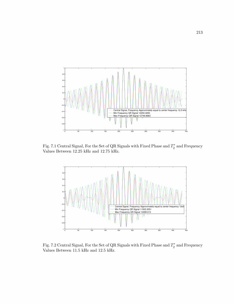
213
0 50 100 150 200 250 300 350 400 450−1
−0.8
−0.6
−0.4
−0.2
0
0.2
0.4
0.6
0.8
1
Central Signal, Frequency Approximately equal to center frequency 12.5 kHz
Min Frequency QR Signal 12250.3293
Max Frequency QR Signal 12749.8963
Fig. 7.1 Central Signal, For the Set of QR Signals with Fixed Phase and T ∗2
and FrequencyValues Between 12.25 kHz and 12.75 kHz.
0 50 100 150 200 250 300 350 400 450−1
−0.8
−0.6
−0.4
−0.2
0
0.2
0.4
0.6
0.8
1
Central Signal, Frequency Approximately equal to center frequency 12e3
Min Frequency QR Signal 11503.3051
Max Frequency QR Signal 12499.013
Fig. 7.2 Central Signal, For the Set of QR Signals with Fixed Phase and T ∗2
and FrequencyValues Between 11.5 kHz and 12.5 kHz.
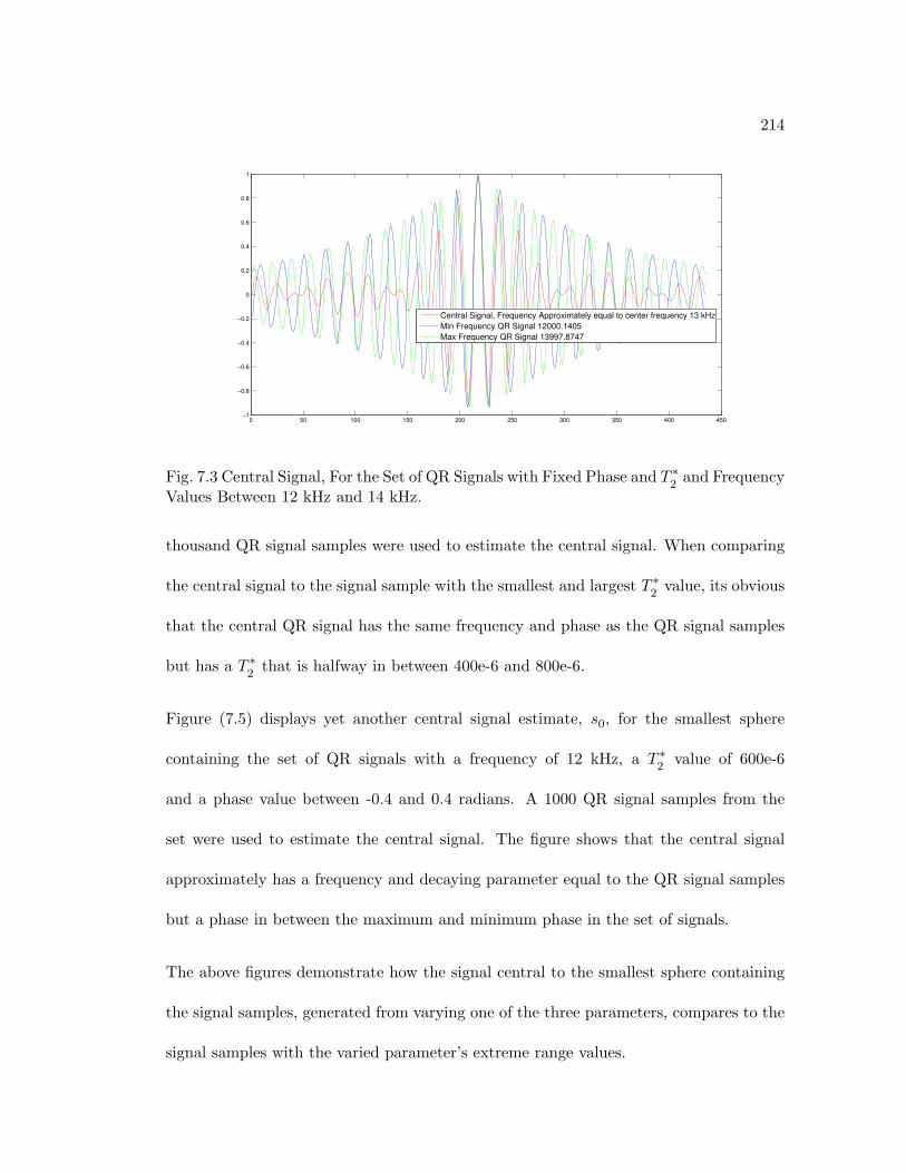
214
0 50 100 150 200 250 300 350 400 450−1
−0.8
−0.6
−0.4
−0.2
0
0.2
0.4
0.6
0.8
1
Central Signal, Frequency Approximately equal to center frequency 13 kHz
Min Frequency QR Signal 12000.1405
Max Frequency QR Signal 13997.8747
Fig. 7.3 Central Signal, For the Set of QR Signals with Fixed Phase and T ∗2
and FrequencyValues Between 12 kHz and 14 kHz.
thousand QR signal samples were used to estimate the central signal. When comparing
the central signal to the signal sample with the smallest and largest T ∗2
value, its obvious
that the central QR signal has the same frequency and phase as the QR signal samples
but has a T ∗2
that is halfway in between 400e-6 and 800e-6.
Figure (7.5) displays yet another central signal estimate, s0, for the smallest sphere
containing the set of QR signals with a frequency of 12 kHz, a T ∗2
value of 600e-6
and a phase value between -0.4 and 0.4 radians. A 1000 QR signal samples from the
set were used to estimate the central signal. The figure shows that the central signal
approximately has a frequency and decaying parameter equal to the QR signal samples
but a phase in between the maximum and minimum phase in the set of signals.
The above figures demonstrate how the signal central to the smallest sphere containing
the signal samples, generated from varying one of the three parameters, compares to the
signal samples with the varied parameter’s extreme range values.
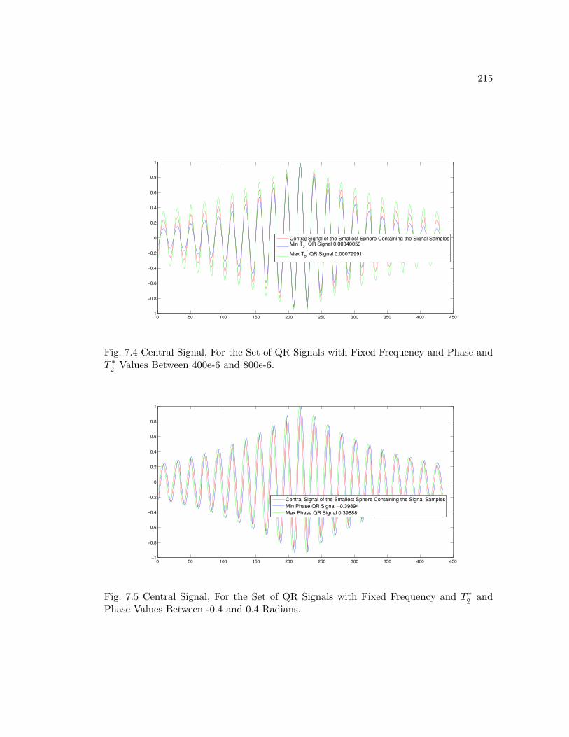
215
0 50 100 150 200 250 300 350 400 450−1
−0.8
−0.6
−0.4
−0.2
0
0.2
0.4
0.6
0.8
1
Central Signal of the Smallest Sphere Containing the Signal SamplesMin T
2
* QR Signal 0.00040059
Max T2
* QR Signal 0.00079991
Fig. 7.4 Central Signal, For the Set of QR Signals with Fixed Frequency and Phase andT ∗
2Values Between 400e-6 and 800e-6.
0 50 100 150 200 250 300 350 400 450−1
−0.8
−0.6
−0.4
−0.2
0
0.2
0.4
0.6
0.8
1
Central Signal of the Smallest Sphere Containing the Signal Samples
Min Phase QR Signal −0.39894
Max Phase QR Signal 0.39888
Fig. 7.5 Central Signal, For the Set of QR Signals with Fixed Frequency and T ∗2
andPhase Values Between -0.4 and 0.4 Radians.
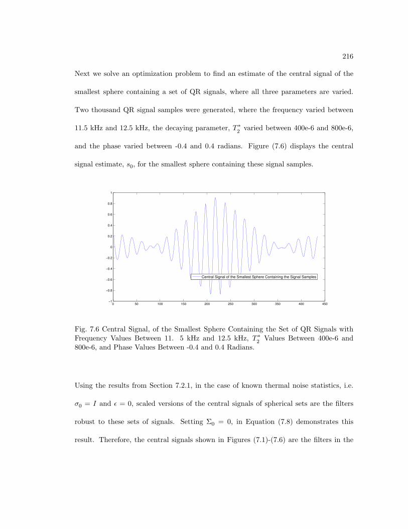
216
Next we solve an optimization problem to find an estimate of the central signal of the
smallest sphere containing a set of QR signals, where all three parameters are varied.
Two thousand QR signal samples were generated, where the frequency varied between
11.5 kHz and 12.5 kHz, the decaying parameter, T ∗2
varied between 400e-6 and 800e-6,
and the phase varied between -0.4 and 0.4 radians. Figure (7.6) displays the central
signal estimate, s0, for the smallest sphere containing these signal samples.
0 50 100 150 200 250 300 350 400 450−1
−0.8
−0.6
−0.4
−0.2
0
0.2
0.4
0.6
0.8
1
Central Signal of the Smallest Sphere Containing the Signal Samples
Fig. 7.6 Central Signal, of the Smallest Sphere Containing the Set of QR Signals withFrequency Values Between 11. 5 kHz and 12.5 kHz, T ∗
2Values Between 400e-6 and
800e-6, and Phase Values Between -0.4 and 0.4 Radians.
Using the results from Section 7.2.1, in the case of known thermal noise statistics, i.e.
σ0 = I and ε = 0, scaled versions of the central signals of spherical sets are the filters
robust to these sets of signals. Setting Σ0 = 0, in Equation (7.8) demonstrates this
result. Therefore, the central signals shown in Figures (7.1)-(7.6) are the filters in the
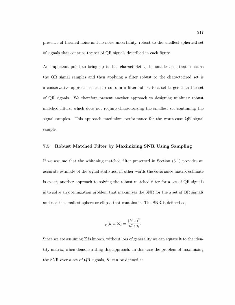
217
presence of thermal noise and no noise uncertainty, robust to the smallest spherical set
of signals that contains the set of QR signals described in each figure.
An important point to bring up is that characterizing the smallest set that contains
the QR signal samples and then applying a filter robust to the characterized set is
a conservative approach since it results in a filter robust to a set larger than the set
of QR signals. We therefore present another approach to designing minimax robust
matched filters, which does not require characterizing the smallest set containing the
signal samples. This approach maximizes performance for the worst-case QR signal
sample.
7.5 Robust Matched Filter by Maximizing SNR Using Sampling
If we assume that the whitening matched filter presented in Section (6.1) provides an
accurate estimate of the signal statistics, in other words the covariance matrix estimate
is exact, another approach to solving the robust matched filter for a set of QR signals
is to solve an optimization problem that maximizes the SNR for the a set of QR signals
and not the smallest sphere or ellipse that contains it. The SNR is defined as,
ρ(h, s,Σ) =(hT s)2
hTΣh.
Since we are assuming Σ is known, without loss of generality we can equate it to the iden-
tity matrix, when demonstrating this approach. In this case the problem of maximizing
the SNR over a set of QR signals, S, can be defined as
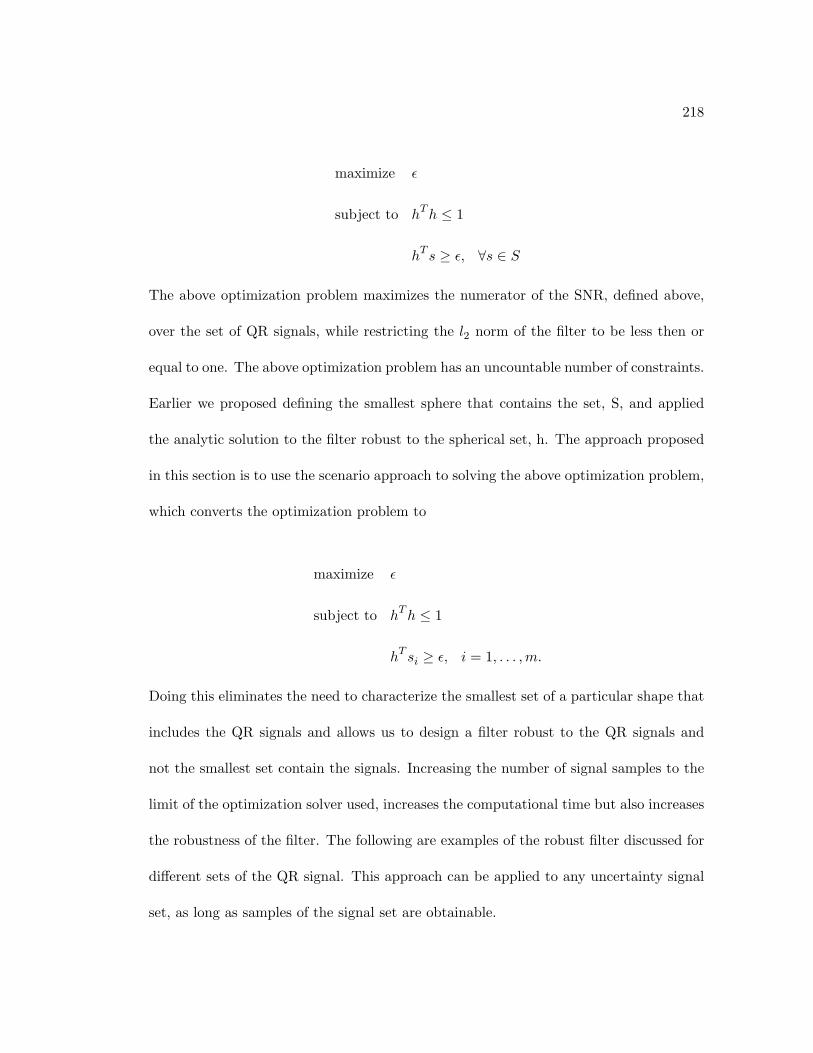
218
maximize ε
subject to hTh ≤ 1
hT s ≥ ε, ∀s ∈ S
The above optimization problem maximizes the numerator of the SNR, defined above,
over the set of QR signals, while restricting the l2 norm of the filter to be less then or
equal to one. The above optimization problem has an uncountable number of constraints.
Earlier we proposed defining the smallest sphere that contains the set, S, and applied
the analytic solution to the filter robust to the spherical set, h. The approach proposed
in this section is to use the scenario approach to solving the above optimization problem,
which converts the optimization problem to
maximize ε
subject to hTh ≤ 1
hT si ≥ ε, i = 1, . . . ,m.
Doing this eliminates the need to characterize the smallest set of a particular shape that
includes the QR signals and allows us to design a filter robust to the QR signals and
not the smallest set contain the signals. Increasing the number of signal samples to the
limit of the optimization solver used, increases the computational time but also increases
the robustness of the filter. The following are examples of the robust filter discussed for
different sets of the QR signal. This approach can be applied to any uncertainty signal
set, as long as samples of the signal set are obtainable.
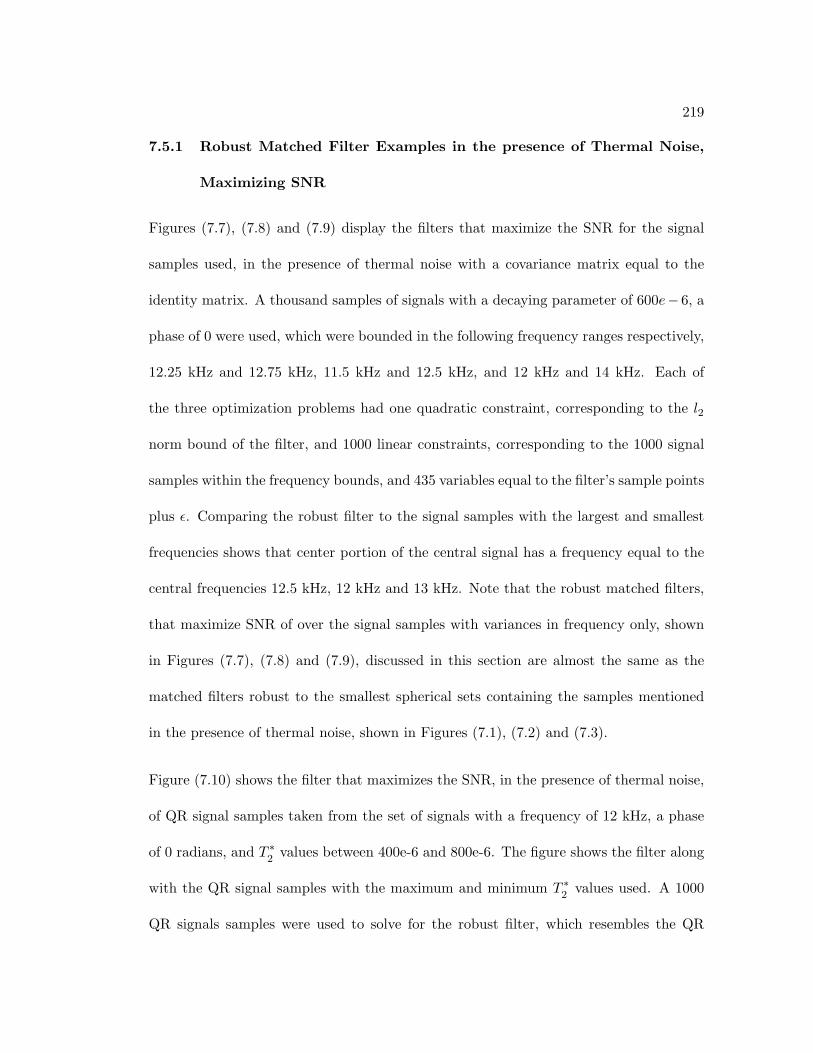
219
7.5.1 Robust Matched Filter Examples in the presence of Thermal Noise,
Maximizing SNR
Figures (7.7), (7.8) and (7.9) display the filters that maximize the SNR for the signal
samples used, in the presence of thermal noise with a covariance matrix equal to the
identity matrix. A thousand samples of signals with a decaying parameter of 600e− 6, a
phase of 0 were used, which were bounded in the following frequency ranges respectively,
12.25 kHz and 12.75 kHz, 11.5 kHz and 12.5 kHz, and 12 kHz and 14 kHz. Each of
the three optimization problems had one quadratic constraint, corresponding to the l2
norm bound of the filter, and 1000 linear constraints, corresponding to the 1000 signal
samples within the frequency bounds, and 435 variables equal to the filter’s sample points
plus ε. Comparing the robust filter to the signal samples with the largest and smallest
frequencies shows that center portion of the central signal has a frequency equal to the
central frequencies 12.5 kHz, 12 kHz and 13 kHz. Note that the robust matched filters,
that maximize SNR of over the signal samples with variances in frequency only, shown
in Figures (7.7), (7.8) and (7.9), discussed in this section are almost the same as the
matched filters robust to the smallest spherical sets containing the samples mentioned
in the presence of thermal noise, shown in Figures (7.1), (7.2) and (7.3).
Figure (7.10) shows the filter that maximizes the SNR, in the presence of thermal noise,
of QR signal samples taken from the set of signals with a frequency of 12 kHz, a phase
of 0 radians, and T ∗2
values between 400e-6 and 800e-6. The figure shows the filter along
with the QR signal samples with the maximum and minimum T ∗2
values used. A 1000
QR signals samples were used to solve for the robust filter, which resembles the QR
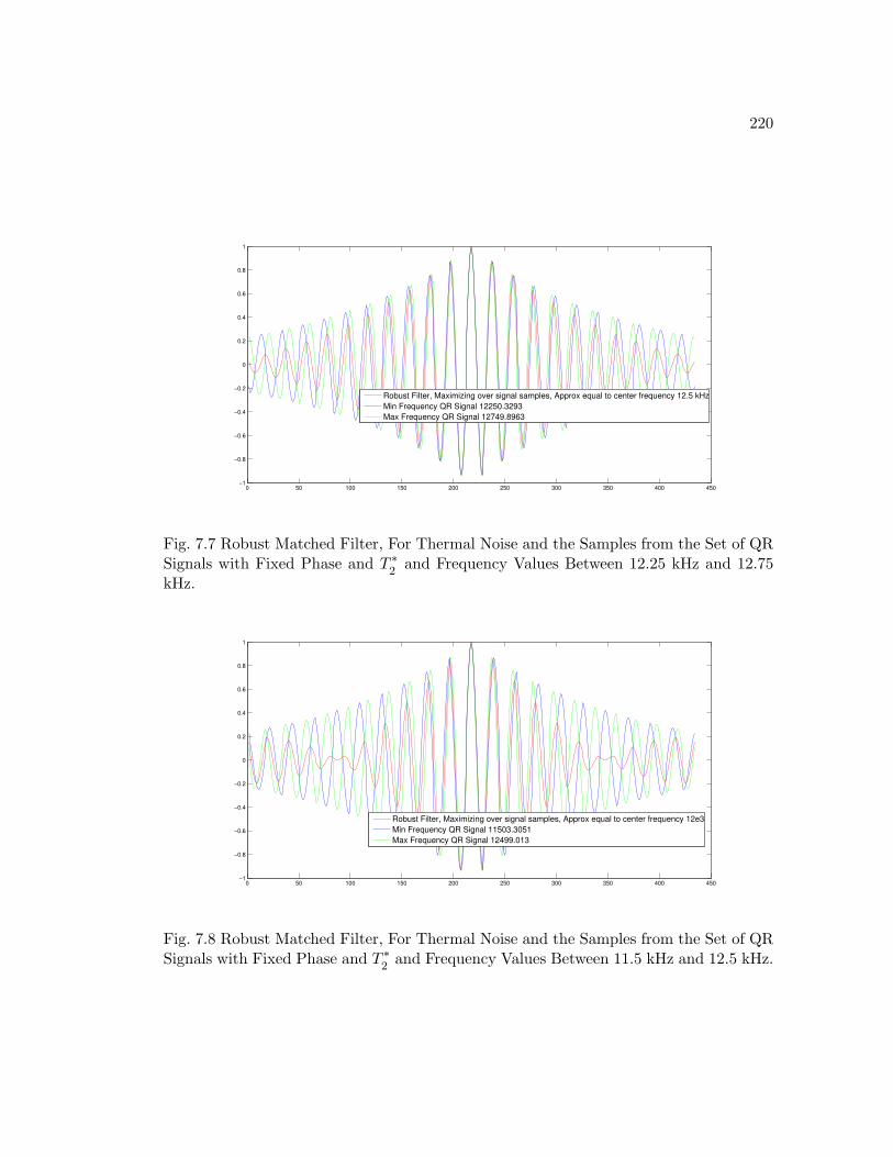
220
0 50 100 150 200 250 300 350 400 450−1
−0.8
−0.6
−0.4
−0.2
0
0.2
0.4
0.6
0.8
1
Robust Filter, Maximizing over signal samples, Approx equal to center frequency 12.5 kHz
Min Frequency QR Signal 12250.3293
Max Frequency QR Signal 12749.8963
Fig. 7.7 Robust Matched Filter, For Thermal Noise and the Samples from the Set of QRSignals with Fixed Phase and T ∗
2and Frequency Values Between 12.25 kHz and 12.75
kHz.
0 50 100 150 200 250 300 350 400 450−1
−0.8
−0.6
−0.4
−0.2
0
0.2
0.4
0.6
0.8
1
Robust Filter, Maximizing over signal samples, Approx equal to center frequency 12e3
Min Frequency QR Signal 11503.3051
Max Frequency QR Signal 12499.013
Fig. 7.8 Robust Matched Filter, For Thermal Noise and the Samples from the Set of QRSignals with Fixed Phase and T ∗
2and Frequency Values Between 11.5 kHz and 12.5 kHz.
221
0 50 100 150 200 250 300 350 400 450−1
−0.8
−0.6
−0.4
−0.2
0
0.2
0.4
0.6
0.8
1
Robust Filter, Maximizing over signal samples, Approx equal to center frequency 13 kHz
Min Frequency QR Signal 12000.1405
Max Frequency QR Signal 13997.8747
Fig. 7.9 Robust Matched Filter, For Thermal Noise and the Samples from the Set of QRSignals with Fixed Phase and T ∗
2and Frequency Values Between 12 kHz and 14 kHz.
signal sample with the lowest T ∗2
value. In this case we see a difference between the filter
discussed above and the filter that would maximize the SNR for the smallest sphere
containing the discussed signal samples, which is shown in Figure (7.4). In that figure,
the central signal to the spherical set (also the robust filter for the spherical set that
contains the QR signal set, in the presence of thermal noise) had a T2∗ value equal to
the central value.
Figure (7.11) shows the filter that maximizes the SNR, in the presence of thermal noise,
of QR signal samples taken from the set of signals with a frequency of 12 kHz, a decaying
parameter, T ∗2
, of 600e-6 and phase values between -0.4 and 0.4 radians. The figure plots
the filter along with the QR signal samples with the maximum and minimum phase
values used. A 1000 QR signal samples were used to solve for the filter, which has a
frequency and decaying parameter equal to the QR signal samples, but a phase value
central to the minimum and maximum phase values that define the set.
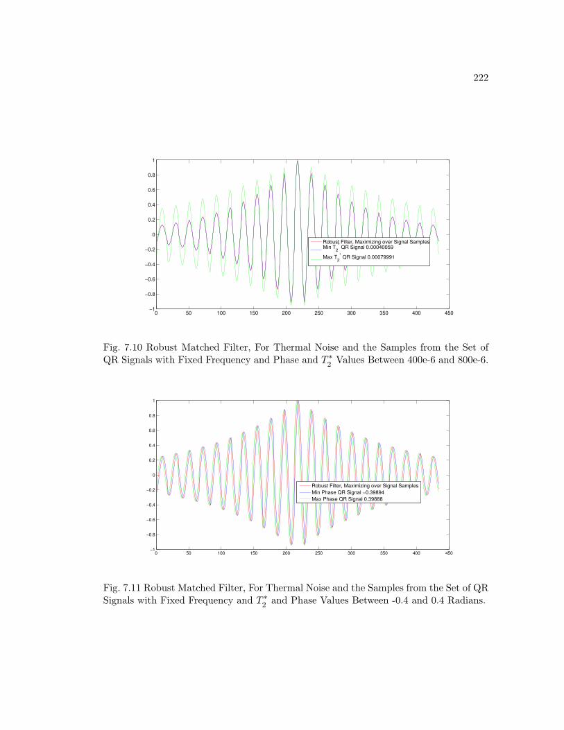
222
0 50 100 150 200 250 300 350 400 450−1
−0.8
−0.6
−0.4
−0.2
0
0.2
0.4
0.6
0.8
1
Robust Filter, Maximizing over Signal SamplesMin T
2
* QR Signal 0.00040059
Max T2
* QR Signal 0.00079991
Fig. 7.10 Robust Matched Filter, For Thermal Noise and the Samples from the Set ofQR Signals with Fixed Frequency and Phase and T ∗
2Values Between 400e-6 and 800e-6.
0 50 100 150 200 250 300 350 400 450−1
−0.8
−0.6
−0.4
−0.2
0
0.2
0.4
0.6
0.8
1
Robust Filter, Maximizing over Signal Samples
Min Phase QR Signal −0.39894
Max Phase QR Signal 0.39888
Fig. 7.11 Robust Matched Filter, For Thermal Noise and the Samples from the Set of QRSignals with Fixed Frequency and T ∗
2and Phase Values Between -0.4 and 0.4 Radians.
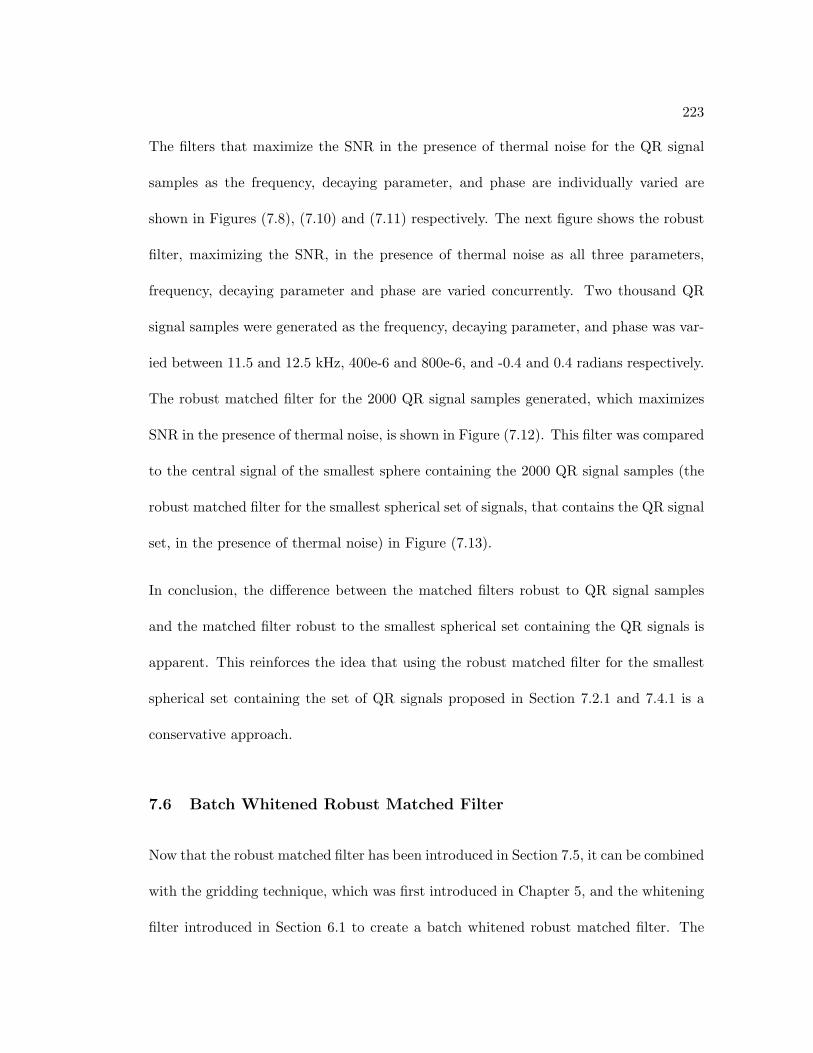
223
The filters that maximize the SNR in the presence of thermal noise for the QR signal
samples as the frequency, decaying parameter, and phase are individually varied are
shown in Figures (7.8), (7.10) and (7.11) respectively. The next figure shows the robust
filter, maximizing the SNR, in the presence of thermal noise as all three parameters,
frequency, decaying parameter and phase are varied concurrently. Two thousand QR
signal samples were generated as the frequency, decaying parameter, and phase was var-
ied between 11.5 and 12.5 kHz, 400e-6 and 800e-6, and -0.4 and 0.4 radians respectively.
The robust matched filter for the 2000 QR signal samples generated, which maximizes
SNR in the presence of thermal noise, is shown in Figure (7.12). This filter was compared
to the central signal of the smallest sphere containing the 2000 QR signal samples (the
robust matched filter for the smallest spherical set of signals, that contains the QR signal
set, in the presence of thermal noise) in Figure (7.13).
In conclusion, the difference between the matched filters robust to QR signal samples
and the matched filter robust to the smallest spherical set containing the QR signals is
apparent. This reinforces the idea that using the robust matched filter for the smallest
spherical set containing the set of QR signals proposed in Section 7.2.1 and 7.4.1 is a
conservative approach.
7.6 Batch Whitened Robust Matched Filter
Now that the robust matched filter has been introduced in Section 7.5, it can be combined
with the gridding technique, which was first introduced in Chapter 5, and the whitening
filter introduced in Section 6.1 to create a batch whitened robust matched filter. The
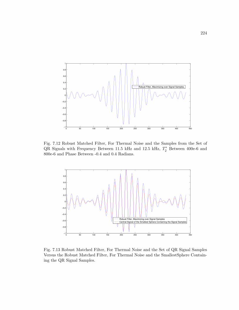
224
0 50 100 150 200 250 300 350 400 450−1
−0.8
−0.6
−0.4
−0.2
0
0.2
0.4
0.6
0.8
1
Robust Filter, Maximizing over Signal Samples,
Fig. 7.12 Robust Matched Filter, For Thermal Noise and the Samples from the Set ofQR Signals with Frequency Between 11.5 kHz and 12.5 kHz, T ∗
2Between 400e-6 and
800e-6 and Phase Between -0.4 and 0.4 Radians.
0 50 100 150 200 250 300 350 400 450−1
−0.8
−0.6
−0.4
−0.2
0
0.2
0.4
0.6
0.8
1
Robust Filter, Maximizing over Signal Samples
Central Signal of the Smallest Sphere Containing the Signal Samples
Fig. 7.13 Robust Matched Filter, For Thermal Noise and the Set of QR Signal SamplesVersus the Robust Matched Filter, For Thermal Noise and the SmallestSphere Contain-ing the QR Signal Samples.
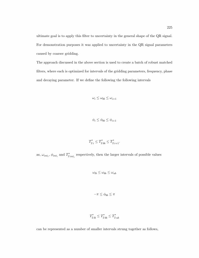
225
ultimate goal is to apply this filter to uncertainty in the general shape of the QR signal.
For demonstration purposes it was applied to uncertainty in the QR signal parameters
caused by coarser gridding.
The approach discussed in the above section is used to create a batch of robust matched
filters, where each is optimized for intervals of the gridding parameters, frequency, phase
and decaying parameter. If we define the following the following intervals
ωi ≤ ωbb ≤ ωi+1
φi ≤ φbb ≤ φi+1
T ∗2 i≤ T ∗
2 bb≤ T ∗
2 i+1.
as, ωinti , φinti and T ∗2 inti
respectively, then the larger intervals of possible values
ωlb ≤ ωbb ≤ ωub
−π ≤ φbb ≤ π
T ∗2 lb≤ T ∗
2 bb≤ T ∗
2 ub
can be represented as a number of smaller intervals strung together as follows,
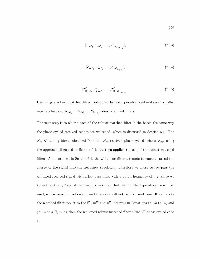
226
[ωint1 , ωint2 , . . . , ωintNintω], (7.13)
[φint1 , φint2 , . . . , φintNφT], (7.14)
[T ∗2 int1
, T ∗2 int2
, . . . , T ∗2 intNintT
]. (7.15)
Designing a robust matched filter, optimized for each possible combination of smaller
intervals leads to Nintω ×Nintφ ×Nintφ robust matched filters.
The next step is to whiten each of the robust matched filter in the batch the same way
the phase cycled received echoes are whitened, which is discussed in Section 6.1. The
Nm whitening filters, obtained from the Nm received phase cycled echoes, xpc, using
the approach discussed in Section 6.1, are then applied to each of the robust matched
filters. As mentioned in Section 6.1, the whitening filter attempts to equally spread the
energy of the signal into the frequency spectrum. Therefore we chose to low pass the
whitened received signal with a low pass filter with a cutoff frequency of ωub, since we
know that the QR signal frequency is less than that cutoff. The type of low pass filter
used, is discussed in Section 6.1, and therefore will not be discussed here. If we denote
the matched filter robust to the lth, mth and nth intervals in Equations (7.13) (7.14) and
(7.15) as sr(l,m, n), then the whitened robust matched filter of the ith phase-cycled echo
is
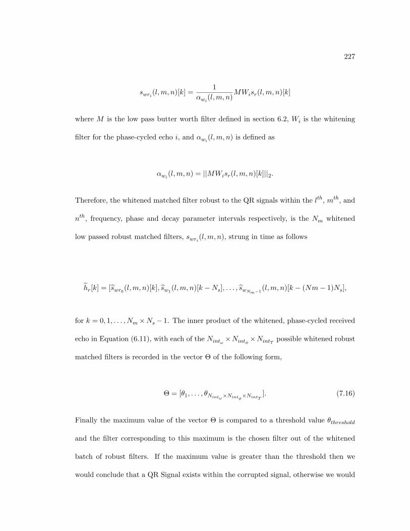
227
swri(l,m, n)[k] =1
αwi(l,m, n)MWisr(l,m, n)[k]
where M is the low pass butter worth filter defined in section 6.2, Wi is the whitening
filter for the phase-cycled echo i, and αwi(l,m, n) is defined as
αwi(l,m, n) = ||MWisr(l,m, n)[k]||2.
Therefore, the whitened matched filter robust to the QR signals within the lth, mth, and
nth, frequency, phase and decay parameter intervals respectively, is the Nm whitened
low passed robust matched filters, swri(l,m, n), strung in time as follows
hr[k] = [swr0(l,m, n)[k], sw1(l,m, n)[k −Ns], . . . , swNm−1
(l,m, n)[k − (Nm− 1)Ns],
for k = 0, 1, . . . , Nm×Ns− 1. The inner product of the whitened, phase-cycled received
echo in Equation (6.11), with each of the Nintω ×Nintφ ×NintT possible whitened robust
matched filters is recorded in the vector Θ of the following form,
Θ = [θ1, . . . , θNintω×Nintφ×NintT]. (7.16)
Finally the maximum value of the vector Θ is compared to a threshold value θthreshold
and the filter corresponding to this maximum is the chosen filter out of the whitened
batch of robust filters. If the maximum value is greater than the threshold then we
would conclude that a QR Signal exists within the corrupted signal, otherwise we would
228
conclude that the received signal is just noise. If using one of the adaptive methods
to whitening, proposed in the previous chapter, gridding through the robust filters is
performed pre whitening and the selected filter is whitened according to the adaptive
whitening algorithm. As was mentioned in the previous chapter determining the value of
θthreshold is still a matter that requires further work. There are several possible ways of
determining the value of θthreshold, one of which, is to collect a measurement of the noise
and use it to determine the value of θthreshold. The next section compares the performance
of the batch robust matched filter, without whitening, to the batch matched filter in the
presence of thermal noise using simulation data. The section following that compares the
performance of the batch whitened robust matched filter to the batch whitened matched
filter in the presence of thermal and AM noise using both simulation data. Both these
filters were whitened with a 6th order whitening filter estimated using the autocorrelation
method.
7.7 Batch Robust Matched Filter in Presence of Thermal Noise
In this section, the performance of the robust matched filter, designed using the approach
above, is compared to the performance of the batch matched filter, discussed in Chapter
5, in the presence of the thermal noise using simulation data. The section starts by
analyzing filters robust to uncertainties in frequencies first, in the following subsection.
The section then moves on to analyzing filters robust to uncertainties in all three QR
signal parameters (frequency, phase and decaying parameter).
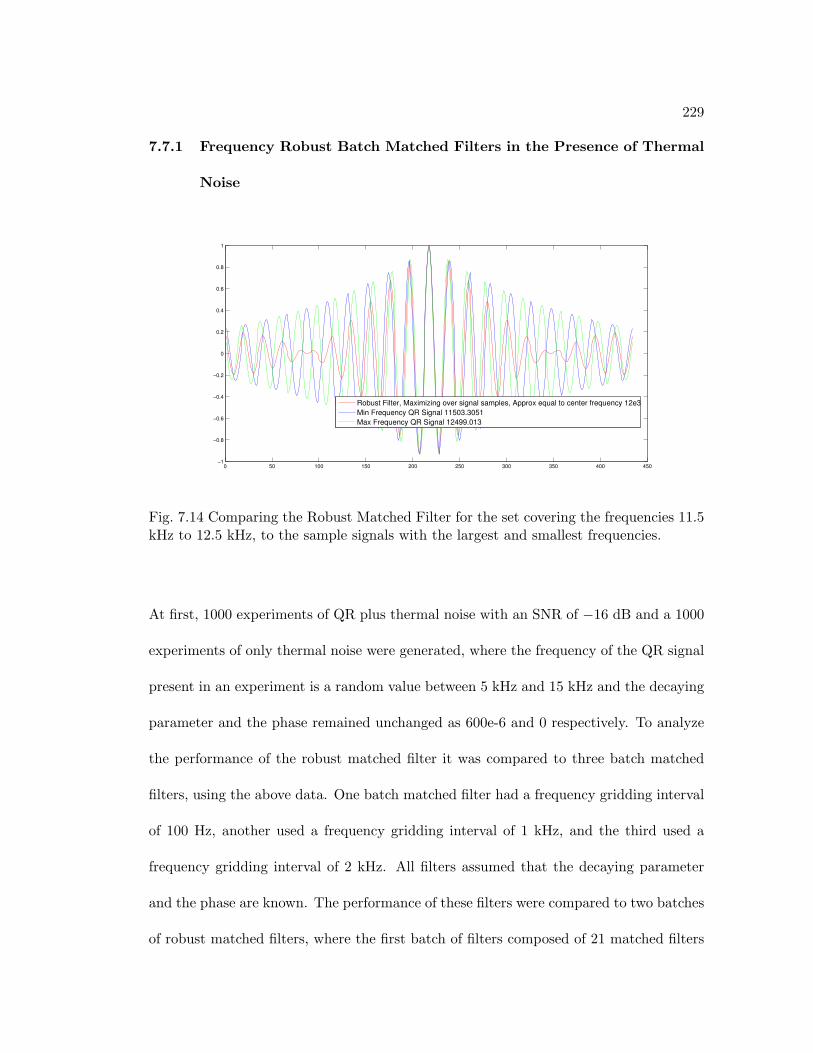
229
7.7.1 Frequency Robust Batch Matched Filters in the Presence of Thermal
Noise
0 50 100 150 200 250 300 350 400 450−1
−0.8
−0.6
−0.4
−0.2
0
0.2
0.4
0.6
0.8
1
Robust Filter, Maximizing over signal samples, Approx equal to center frequency 12e3
Min Frequency QR Signal 11503.3051
Max Frequency QR Signal 12499.013
Fig. 7.14 Comparing the Robust Matched Filter for the set covering the frequencies 11.5kHz to 12.5 kHz, to the sample signals with the largest and smallest frequencies.
At first, 1000 experiments of QR plus thermal noise with an SNR of −16 dB and a 1000
experiments of only thermal noise were generated, where the frequency of the QR signal
present in an experiment is a random value between 5 kHz and 15 kHz and the decaying
parameter and the phase remained unchanged as 600e-6 and 0 respectively. To analyze
the performance of the robust matched filter it was compared to three batch matched
filters, using the above data. One batch matched filter had a frequency gridding interval
of 100 Hz, another used a frequency gridding interval of 1 kHz, and the third used a
frequency gridding interval of 2 kHz. All filters assumed that the decaying parameter
and the phase are known. The performance of these filters were compared to two batches
of robust matched filters, where the first batch of filters composed of 21 matched filters
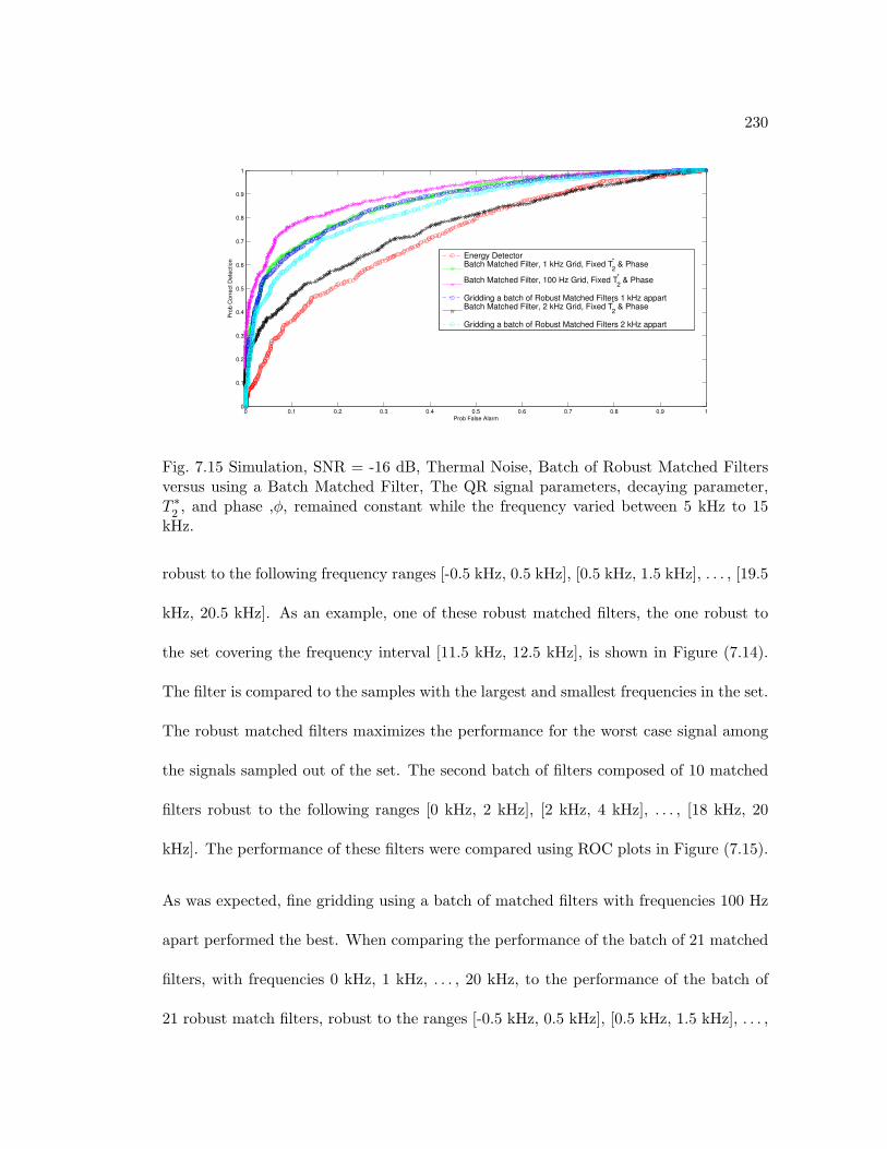
230
0 0.1 0.2 0.3 0.4 0.5 0.6 0.7 0.8 0.9 10
0.1
0.2
0.3
0.4
0.5
0.6
0.7
0.8
0.9
1
Pro
b C
orr
ect D
ete
ction
Prob False Alarm
Energy DetectorBatch Matched Filter, 1 kHz Grid, Fixed T
2
* & Phase
Batch Matched Filter, 100 Hz Grid, Fixed T2
* & Phase
Gridding a batch of Robust Matched Filters 1 kHz appartBatch Matched Filter, 2 kHz Grid, Fixed T
2
* & Phase
Gridding a batch of Robust Matched Filters 2 kHz appart
Fig. 7.15 Simulation, SNR = -16 dB, Thermal Noise, Batch of Robust Matched Filtersversus using a Batch Matched Filter, The QR signal parameters, decaying parameter,T ∗
2, and phase ,φ, remained constant while the frequency varied between 5 kHz to 15
kHz.
robust to the following frequency ranges [-0.5 kHz, 0.5 kHz], [0.5 kHz, 1.5 kHz], . . . , [19.5
kHz, 20.5 kHz]. As an example, one of these robust matched filters, the one robust to
the set covering the frequency interval [11.5 kHz, 12.5 kHz], is shown in Figure (7.14).
The filter is compared to the samples with the largest and smallest frequencies in the set.
The robust matched filters maximizes the performance for the worst case signal among
the signals sampled out of the set. The second batch of filters composed of 10 matched
filters robust to the following ranges [0 kHz, 2 kHz], [2 kHz, 4 kHz], . . . , [18 kHz, 20
kHz]. The performance of these filters were compared using ROC plots in Figure (7.15).
As was expected, fine gridding using a batch of matched filters with frequencies 100 Hz
apart performed the best. When comparing the performance of the batch of 21 matched
filters, with frequencies 0 kHz, 1 kHz, . . . , 20 kHz, to the performance of the batch of
21 robust match filters, robust to the ranges [-0.5 kHz, 0.5 kHz], [0.5 kHz, 1.5 kHz], . . . ,
231
[19.5, 20.5 kHz], their performance is more or less equal. The performance of these two
detectors are shown in the green and blue curves. As the frequency intervals between
filters in the batch of matched filters increased the performance of the batch of matched
filters decreased. This is apparent when comparing the black curve, where the batch of
matched filters are 2 kHz apart, to the green curve, where the batch of filters are only 1
kHz apart. Though as the interval of frequencies the robust matched filter is robust to is
increased from 1 kHz (the blue curve) to 2 kHz (the cyan curve), the performance drop
is insignificant when compared to the drop seen when using batch matched filters. Since
the robust matched filters that are robust to 2 kHz frequency intervals cover twice the
range of frequencies as the robust matched filters robust to 1 kHz intervals, the number
of filters required in the batch to cover the complete range of frequencies is reduced by a
factor of two leading to half the computation time required. Therefore, if computation
time is a factor and fine gridding is not an option then using a batch of robust matched
filter is superior to using a batch of matched filters, which is apparent when comparing
the cyan curve to the black curve.
7.7.2 Robust Batch Matched Filters in the Presence of Thermal Noise
Another set of data was generated was generated, where the QR signals varied in fre-
quency, phase and decaying parameter and not only frequency. A 1000 experiments of
QR plus thermal noise and 1000 experiments of only thermal noise were generated. The
QR signal present at a given experiment, had a random frequency varied between 5 kHz
and 15 kHz, a random phase between −π/2 and π/2 and a random decaying parameter
232
between 400e-6 and 800e-6. This data was used to compare the performance of two batch
robust matched filters and three batch matched filters in Figure (7.16).
As expected, the best performing filter was the batch matched filter with a fine grid
of, 100 Hz, 0.1 radians and 100e-6 in between grid ding values for frequency, phase and
decaying parameter respectively. Such a batch of filters consists of Ndω ×Ndφ ×NdT =
201× 63× 5 = 63, 315 filters, which is the largest batch among filters compared in this
figure. The in-between grid values for frequency, phase, and decaying parameter for the
other two filters were 1 kHz, 0.2 radians, and 200e-6 respectively for one, and 2 kHz,
0.2 radians, and 200e-6 for the other. The number of filters in the above two batches of
matched filters were Ndω × Ndφ × NdT = 21 × 32 × 3 = 2016 and Ndω × Ndφ × NdT =
11× 32× 3 = 1056 respectively. Figure (7.16) shows that as the values in-between grid
parameters of the batch matched filters increased the performance dropped, which is
apparent from comparing the magenta, green and black curves. The first batch robust
matched filter used consisted of a group of filters robust to QR signals with frequency,
phase and decaying parameter that fall within the intervals of size 1 kHz, 0.2 radians and
200e-6 respectively. This batch robust matched filter consists of Nintω ×Nintφ ×NintT =
20× 32× 3 = 1920, individual filters, which is comparable to the number of filters in the
batch matched filter with 2 kHz spacing in-between frequency values. Comparing the
green curve to the blue curve shows that in this case the batch matched filter and the
batch robust matched filter have approximately equal performance. The second batch
robust matched filter consisted of a group of filters robust to QR signals with frequency,
phase and decaying parameter that fall within the intervals size 2 kHz, 0.2 radians and
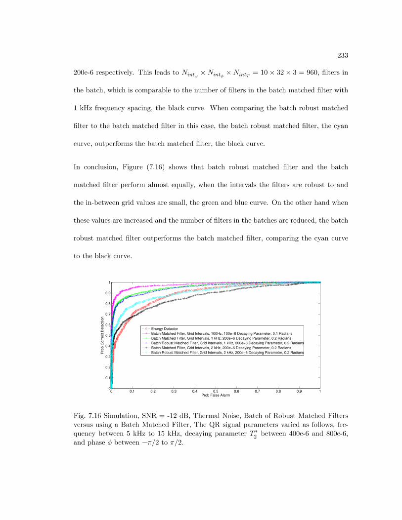
233
200e-6 respectively. This leads to Nintω ×Nintφ ×NintT = 10 × 32 × 3 = 960, filters in
the batch, which is comparable to the number of filters in the batch matched filter with
1 kHz frequency spacing, the black curve. When comparing the batch robust matched
filter to the batch matched filter in this case, the batch robust matched filter, the cyan
curve, outperforms the batch matched filter, the black curve.
In conclusion, Figure (7.16) shows that batch robust matched filter and the batch
matched filter perform almost equally, when the intervals the filters are robust to and
the in-between grid values are small, the green and blue curve. On the other hand when
these values are increased and the number of filters in the batches are reduced, the batch
robust matched filter outperforms the batch matched filter, comparing the cyan curve
to the black curve.
0 0.1 0.2 0.3 0.4 0.5 0.6 0.7 0.8 0.9 10
0.1
0.2
0.3
0.4
0.5
0.6
0.7
0.8
0.9
1
Pro
b C
orr
ect D
ete
ction
Prob False Alarm
Energy Detector
Batch Matched Filter, Grid Intervals, 100Hz, 100e−6 Decaying Parameter, 0.1 Radians
Batch Matched Filter, Grid Intervals, 1 kHz, 200e−6 Decaying Parameter, 0.2 Radians
Batch Robust Matched Filter, Grid Intervals, 1 kHz, 200e−6 Decaying Parameter, 0.2 Radians
Batch Matched Filter, Grid Intervals, 2 kHz, 200e−6 Decaying Parameter, 0.2 Radians
Batch Robust Matched Filter, Grid Intervals, 2 kHz, 200e−6 Decaying Parameter, 0.2 Radians
Fig. 7.16 Simulation, SNR = -12 dB, Thermal Noise, Batch of Robust Matched Filtersversus using a Batch Matched Filter, The QR signal parameters varied as follows, fre-quency between 5 kHz to 15 kHz, decaying parameter T ∗
2between 400e-6 and 800e-6,
and phase φ between −π/2 to π/2.
234
7.8 Batch Whitened Robust Matched Filter in the Presence of AM
and Thermal Noise
The purpose of this section is to compare gridding using filters robust to sets of QR
signals with varying QR parameters versus gridding using filters matched to specific
QR signals, in the presence of AM and thermal noise. The section compares the two
detectors, the batch whitened matched filter and the batch whitened robust matched
filter using simulation data. The section then moves on to demonstrating why comparing
the filters using the available experimental data is aimless.
7.8.1 Simulation Data in the Presence of AM and Thermal Noise
The simulation data used in this section was a 1000 experiments of QR plus AM and
thermal noise and a 1000 experiments of only AM and thermal noise. The QR signal
present in an experiment had a frequency that varied between 5 kHz and 15 kHz, a
phase between −π/2 and π/2, and a decaying parameter between 400e-6 and 800e-6.
The carrier of the AM signal present in an experiment had a fixed frequency of 10 kHz.
To start, this data was used to compare the performance of two batch robust matched
filters and three batch matched filters in Figure (7.17). The same data is then used
to compare the performance of the batch whitened robust matched filter to the batch
whitened matched filter in Figure (7.18).
In Figure (7.17) the best performing filter, was the batch matched filter with a fine grid
of, 100 Hz, 0.1 radians and 100e-6 in between gridding values for frequency, phase and
decaying parameter respectively. As was stated above, this batch of filters consists of
235
Ndω ×Ndφ ×NdT = 201× 63× 5 = 63, 315 filters and therefore this filter has the largest
computational time. The in-between grid values for frequency, phase, and decaying
parameter for the other two filters were 1 kHz, 0.2 radians, and 200e-6 respectively for
one, and 2 kHz, 0.2 radians, and 200e-6 for the other. The number of filters in the
above two batches of matched filters were Ndω ×Ndφ ×NdT = 21 × 32 × 3 = 2016 and
Ndω ×Ndφ ×NdT = 11× 32× 3 = 1056 respectively.
The first batch robust matched filter used consisted of a group of filters robust to QR
signals with frequency, phase and decaying parameter that fall within the intervals of size
1 kHz, 0.2 radians and 200e-6 respectively. This batch robust matched filter consists of
Nintω ×Nintφ×NintT = 20×32×3 = 1920, individual filters, which is comparable to the
number of filters in the batch matched filter with 1 kHz spacing in-between frequency
values. Comparing the green curve to the blue curve shows that in this case the batch
matched filter and the batch robust matched filter have more or less equal performance.
The second batch robust matched filter consisted of a group of filters robust to QR signals
with frequency, phase and decaying parameter that fall within intervals of size 2 kHz, 0.2
radians and 200e-6 respectively. This leads to Nintω ×Nintφ×NintT = 10×32×3 = 960,
filters in the batch, which is comparable to the number of filters in the batch matched
filter with 2 kHz frequency spacing, the black curve. When comparing the batch robust
matched filter to the batch matched filter in this case, the batch robust matched filter,
the cyan curve, outperforms the batch matched filter, the black curve. Next these filters
will integrate the whitening approach and their performance will be compared using the
same set of data.
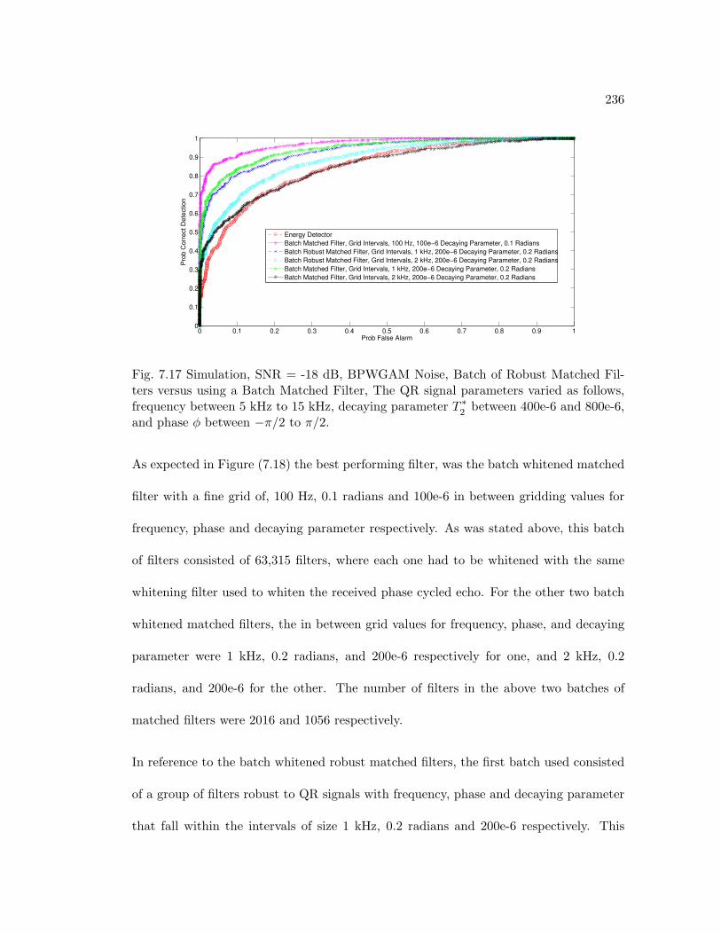
236
0 0.1 0.2 0.3 0.4 0.5 0.6 0.7 0.8 0.9 10
0.1
0.2
0.3
0.4
0.5
0.6
0.7
0.8
0.9
1
Pro
b C
orr
ect D
ete
ction
Prob False Alarm
Energy Detector
Batch Matched Filter, Grid Intervals, 100 Hz, 100e−6 Decaying Parameter, 0.1 Radians
Batch Robust Matched Filter, Grid Intervals, 1 kHz, 200e−6 Decaying Parameter, 0.2 Radians
Batch Robust Matched Filter, Grid Intervals, 2 kHz, 200e−6 Decaying Parameter, 0.2 Radians
Batch Matched Filter, Grid Intervals, 1 kHz, 200e−6 Decaying Parameter, 0.2 Radians
Batch Matched Filter, Grid Intervals, 2 kHz, 200e−6 Decaying Parameter, 0.2 Radians
Fig. 7.17 Simulation, SNR = -18 dB, BPWGAM Noise, Batch of Robust Matched Fil-ters versus using a Batch Matched Filter, The QR signal parameters varied as follows,frequency between 5 kHz to 15 kHz, decaying parameter T ∗
2between 400e-6 and 800e-6,
and phase φ between −π/2 to π/2.
As expected in Figure (7.18) the best performing filter, was the batch whitened matched
filter with a fine grid of, 100 Hz, 0.1 radians and 100e-6 in between gridding values for
frequency, phase and decaying parameter respectively. As was stated above, this batch
of filters consisted of 63,315 filters, where each one had to be whitened with the same
whitening filter used to whiten the received phase cycled echo. For the other two batch
whitened matched filters, the in between grid values for frequency, phase, and decaying
parameter were 1 kHz, 0.2 radians, and 200e-6 respectively for one, and 2 kHz, 0.2
radians, and 200e-6 for the other. The number of filters in the above two batches of
matched filters were 2016 and 1056 respectively.
In reference to the batch whitened robust matched filters, the first batch used consisted
of a group of filters robust to QR signals with frequency, phase and decaying parameter
that fall within the intervals of size 1 kHz, 0.2 radians and 200e-6 respectively. This
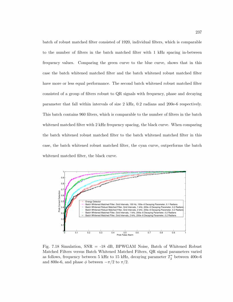
237
batch of robust matched filter consisted of 1920, individual filters, which is comparable
to the number of filters in the batch matched filter with 1 kHz spacing in-between
frequency values. Comparing the green curve to the blue curve, shows that in this
case the batch whitened matched filter and the batch whitened robust matched filter
have more or less equal performance. The second batch whitened robust matched filter
consisted of a group of filters robust to QR signals with frequency, phase and decaying
parameter that fall within intervals of size 2 kHz, 0.2 radians and 200e-6 respectively.
This batch contains 960 filters, which is comparable to the number of filters in the batch
whitened matched filter with 2 kHz frequency spacing, the black curve. When comparing
the batch whitened robust matched filter to the batch whitened matched filter in this
case, the batch whitened robust matched filter, the cyan curve, outperforms the batch
whitened matched filter, the black curve.
0 0.1 0.2 0.3 0.4 0.5 0.6 0.7 0.8 0.9 10
0.1
0.2
0.3
0.4
0.5
0.6
0.7
0.8
0.9
1
Pro
b C
orr
ect D
ete
ction
Prob False Alarm
Energy Detector
Batch Whitened Matched Filter, Grid Intervals, 100 Hz, 100e−6 Decaying Parameter, 0.1 Radians
Batch Whitened Robust Matched Filter, Grid Intervals, 1 kHz, 200e−6 Decaying Parameter, 0.2 Radians
Batch Whitened Robust Matched Filter, Grid Intervals, 2 kHz, 200e−6 Decaying Parameter, 0.2 Radians
Batch Whitened Matched Filter, Grid Intervals, 1 kHz, 200e−6 Decaying Parameter, 0.2 Radians
Batch Whitened Matched Filter, Grid Intervals, 2 kHz, 200e−6 Decaying Parameter, 0.2 Radians
Fig. 7.18 Simulation, SNR = -18 dB, BPWGAM Noise, Batch of Whitened RobustMatched Filters versus Batch Whitened Matched Filters, QR signal parameters variedas follows, frequency between 5 kHz to 15 kHz, decaying parameter T ∗
2between 400e-6
and 800e-6, and phase φ between −π/2 to π/2.
238
Simulation results, have shown that in cases of fine gridding, a batch whitened robust
matched filter and a batch whitened matched filter, with a comparable number of filters
in the batch, perform more or less equally and therefore robustness in the QR signal
parameters is unnecessary. Though the ultimate aim of robust filters is to be applied to
uncertainty in the QR signal shape, while fine gridding in the QR signal parameters. In
cases of unfine gridding in the QR signal parameters the batch whitened robust (robust
to QR signal parameters) matched filter outperforms a batch whitened matched filter,
with a comparable number of filters in the batch. Therefore, the batch whitened robust
matched filter (robust to uncertainties in the QR signal parameters) should only replace
the batch whitened matched filter, when fine gridding of the QR parameters is not an
option. In this case decreasing the number of filters in the batch of whitened robust
matched filters, does not degrade performance the performance as it does for the batch
whitened matched filter.
Unfortunately due to the lack of experimental data with varying QR signal parameters,
this phenomena can not be tested on experimental data and the following section explains
why.
7.8.2 Experimental Data in the Presence of AM and Thermal Noise
The goal of the robust matched filter is to optimize performance for a set of QR signals.
The set represents uncertainty in the signal and can be in the general shape of the QR
signal or in the QR parameters. The experimental data collected lacks this uncertainty
or variance in the QR parameter or the signal’s general shape so it is pointless to use to
analyze the performance of robust filters. Using simulation data above we generated QR
239
signals with varying QR signal parameter and we have shown that on average a batch
of robust filters, robust to uncertainties in QR signal parameters, should only be used
when fine grading can not be used.
The experimental data collected for this thesis consisted of four different sets of data,
where each set’s QR signal had a fixed frequency, phase and decaying parameter. The
lack of variance in the QR signal parameters of the experimental data, prevents us from
properly comparing the performance of the batch whitened robust matched to the batch
whitened matched filter. The following example illustrates this point.
Let the experimental set contain a QR signal with frequency, phase and decaying pa-
rameter of 12.1 kHz, 0 radians and 500e-6 respectively. To illustrate, let us assume he
following five batches of whitened filters are applied, where the first three are matched
filters and the last two are robust matched filters.
1. In between grid values: frequency ω∆ = 2π×100, phase φ∆ = 0.1 radians, decaying
parameter T ∗2 ∆
= 100e− 6.
2. In between grid values: frequency ω∆ = 2π × 1000, phase φ∆ = 0.2 radians,
decaying parameter T ∗2 ∆
= 200e− 6.
3. In between grid values: frequency ω∆ = 2π × 2000, phase φ∆ = 0.2 radians,
decaying parameter T ∗2 ∆
= 200e− 6.
4. Filters robust to intervals of length: frequency 2π × 1000, phase 0.2 radians, de-
caying parameter 200e-6.
240
5. Filters robust to intervals of length: frequency 2π × 2000, phase 0.2 radians, de-
caying parameter 200e-6.
From the discussion of batch robust matched filters in Chapter 6, we would expect the
performance of the batch of filters on average to drop as the in between grid values
increase. Therefore, the first batch is expected perform better than the second and the
second is expected to perform better than the third, as the QR signal parameters varied.
Though, since the frequency, phase and decaying parameter of the QR signal present in
the example above are fixed to 12 kHz, 0 radians, and 500e-6, its parameters are always
100 Hz, 0.1 radians, and 100e-6 away from one of the filters in the batch, for both the
second and third batch. Therefore the performance of the second batch should not be
significantly better than the third one.
On the other hand when comparing the last two batches of whitened robust matched
filters to each other, the first batch will always outperform the second batch since the
second batch of filters are robust to larger sets of signals. The second and fourth batch of
filters contain almost the same number of filters, while the third and fifth batch contain
almost the same number of filters.
In other words, for QR signals with random signal parameters, increasing the in between
grid values when using a batch whitened matched filter, and increasing the length of the
intervals the filters are robust to when using a batch whitened robust matched filter,
causes a drop in performance. On the other hand, when the QR signal parameters of the
signal present are fixed (the case with experimental data) this is not always the case. For
specific cases, where the distance of the signal’s parameters to the parameters of one of
241
the filters remain unchanged, increasing the in between grid values does significantly drop
performance. Therefore, to properly compare the performance of the batch whitened
matched filter to the batch of whitened robust matched filter a set of QR signals with
random parameters is needed.
The batch whitened robust matched filter discussed in this chapter can be applied to any
uncertainty in the QR signal parameters. As mentioned earlier, the ultimate goal is to
apply this filter to uncertainty the general shape of the QR signal and use fine gridding
to minimize uncertainty in the QR signal parameters.
242
Chapter 8
Conclusion
In conclusion, the matched filter approaches to QR signal detection, proposed in this
thesis, have shown significant improvements over the generic energy detector. Among
the different matched filter approaches, the batch whitened matched filter (discussed in
Chapter 6) with a properly chosen filter order performed best.
The motivation behind using a matched filter approach was presented in Chapter 4
by comparing the test statistic of the matched filter, under the assumption that the
QR signal is known, to that of the energy detector. This is an unrealistic case, but it
demonstrated an advantage to using a matched filter approach in QR detection. The
distributions of the test statistics in the presence of a QR signal and in the absence of
one, are more separable in the case of the matched filter when compared to the energy
detector.
This was followed by Chapter 5, which presented a gridding approach to the matched
filter referred to as the batch matched filter, which does not assume any knowledge
about the QR signal present. The approach utilizes the knowledge that the unknown
QR signal parameters, frequency, phase and decaying parameter, fall within lower and
upper bounds and discretizes the interval of admissible values to create a finite set of
possible values, for each of the QR signal parameters. These sets, one for each of the three
QR signal parameters, form a grid, where each point refers to a possible combination of
243
values for the QR signal parameters. The number of points on grid is dependent on the
number of discrete values in each of the three QR signal parameters. A set of filters are
then designed, where each is matched to one of the grid points, which are used to detect
the presence of the QR signal. The performance of this filter is dependent on how finely
discretized the unknown QR signal parameters are. A finely gridded batch matched
filter significantly outperforms the energy detector, though it has been shown that the
improvement gained from fine gridding reaches a point of saturation. The computational
time increases as the grid becomes finer. This chapter also introduces an adaptive way
to gridding that can significantly reduce the number of filters in a batch and achieve the
same performance as the brute force method. The adaptive method performs a global
coarser grid search, which is followed by a local finer grid around the grid point selected
by the global grid. Another important point to make, is the fact that the batch matched
filter is ignorant to the type of noise present and does not utilize any information about
the noise in detecting the QR signal.
The filter discussed above is then combined with a whitening filter in Chapter 6, resulting
in a filter referred to as the batch whitened matched. The whitening filter is the inverse
of the noise model estimate, estimated under the assumption that the present noise is
wide sense stationary across the length of an echo, and uses it to whiten the received
signal and the batch of filters. The WSS assumption is a reasonable one, since the length
of an echo is less than 2 ms. As was shown in Chapter 6, estimating a whitening filter
is equivalent to estimating the covariance matrix of the noise present, since one can
be derived from the other. With the properly chosen whitening filter order, this filter
244
outperformed both the batch matched filter and the energy detector, which was expected
since it not only attempts to match to the QR signal present but also the noise statistics.
In estimating the whitening filter the chapter proposed two methods, the autocorrelation
and the covariance methods. The chapter also proposed an adaptive method to selecting
the whitening filter, the first would select the whitening filter order that would least
affect the QR signal while the second used the minimum description length algorithm
to select the filter order. The chapter compared the adaptive methods to selecting the
whitening filter, by comparing the batch whitened matched filters, whitened with a filter
of order chosen by one of the adaptive order selecting methods and estimated using one
of the modeling estimates. This results in four different filters, and according to the
experimental data, the filter that used the covariance method to model the filter with
an order that least affects the QR signal consistently outperformed the batch matched
filter. The results from the simulation data did not point to one filter that consistently
outperformed the remaining filters. Integrating the whitening filter with the gridding
approach further increases the computational time required for the filter to make a
decision, since not only is the received signal whited but so is each of the filters in the
batch. Though this can be significantly reduced by using the adaptive gridding approach
introduced in Chapter 5.
Chapter 7 presents the batch whitened robust matched filter, which combines the whiten-
ing filter with a batch of robust matched filter, where each optimizes SNR for a set of
QR signals instead of a single signal. The ultimate goal is to design a batch of filters,
each matched to particular QR signal parameters, robust to uncertainty in the general
245
shape of the signal. Finely gridding the QR signal parameters reduces the effect of un-
certainty in the QR signal parameters, and therefore robustness to QR signal parameters
is unnecessary. Due to the lack of experimental data with variances in the general shape
of the QR signal, designing filters robust to uncertainty in the general shape QR signal
was not possible. The chapter lays out the tools needed to design a batch of whitened
robust (robust to uncertainty in general QR signal shape) matched filters. For demon-
stration, the chapter compared the performance of the batch whitened matched filter to
the batch whitened robust (robust to uncertainty in QR parameters) matched filter, and
has shown that when fine gridding can be performed robustness to the QR parameters
is unnecessary.
The scenario approach, used in the designing filters robust to variances in the QR pa-
rameters can be used in designing filters robust to any type of uncertainty in the QR
signal, as long as signal samples are obtainable. Variances in the general shape in the
QR signal can be caused by narrow bandwidth filters and coils.
8.1 Future Work
There are several areas one can further address, which will be discussed in this section.
One of which is to further analyze the modeling methods used to estimate the noise
models. Another, is to further analyze the adaptive methods used to choosing the
whitening filter order. These two points can help one develop a method, where the
output of the four different batch adaptive whitened matched filters compared in Section
(6.4) can be used to determine the presence of a QR signal. This idea stems from the
246
fact that for any of the data sets (simulation and experimental) used to compare the
four filters, at least one outperformed the batch matched filter.
Further work also needs to be done with the regards to the robust filters. First, experi-
mental data with variances in the general shape of the QR signal needs to be collected.
This data can be used as signal samples to design filters robust to variances in the general
shape of the QR signal. The performance of these robust filters should then be compared
to the performance of the matched filters using data with variances in the general QR
signal shape.
247
Appendix A
Mean and Variance of Energy Detector Test Statistic,
in the Presence of AM and Thermal Noise
From section (4.1) the test statistic of the energy detector is of the following form
T (x) =Ns−1∑k=0
x[k]2, (A.1)
where x[k] is the received signal. The test statistic is the sum of Ns independent random
variables and since Ns is large, it can be approximated as a gaussian random variable.
To find the mean and variance of the test statistic, we first have to find the mean and
variance of the received signal squared for a certain value of k, x[k]2.
Under the assumption that received signal is the sum of averaged QR, AM and thermal
signals, the received signal squared for a certain value of k is equal to,
x2[k] =s2avg
[k] + η2avg
[k] + n2avg
[k] + 2savg[k]ηavg[k]
+ 2savg[k]navg[k] + 2ηavg[k]navg[k]
248
where navg[k] is a random variable and has the distribution N(0, σ2avg,tn
). The variable
ηavg[k] is also a normal random variable that is also a function of the random phase of
the AM signal, φ. The first moment of the random variable ηavg[k], µη[k], is
µη[k] =Aη
2NeNm
Nm−1∑i=0
Ne∑j=1
[cos (∆ωAM (D(i, j, k) + φ)− (A.2)
cos (∆ωAM (D(i, j, k) + τd) + φ)]
while the second moment, σ2η[k], is
σ2η[k] =E{η2
avg[k]} − µ2
η[k] (A.3)
=
(A2η
(2NeNm)2
)E
Nm−1∑
i=0
Ne∑j=1
(1 +m[D(i, j, k)]) cos (∆ωAM (D(i, j, k)) + φ)−
(1 +m[D(i, j, k)]) cos (∆ωAM (D(i, j, k) + τd) + φ)
)2−(
A2η
(2NeNm)2
)Nm−1∑i=0
Ne∑j=1
cos (∆ωAM (D(i, j, k)) + φ)−
cos (∆ωAM (D(i, j, k) + τd) + φ)
)2
=
(A2η
(2NeNm)2
)Nm−1∑i=0
Ne∑j=1
σ2m
[cos2 (∆ωAM (D(i, j, k) + φ)+
cos2 (∆ωAM (D(i, j, k) + τd) + φ)]
249
Since the first and second moments of a normal random variable completely describe the
distribution, we can move on to calculating the mean and variance of the received signal
squared for a certain value k, x2[k]. The mean value of the received signal squared,
µx2 [k], as a function of k, would be
µx2 [k] = E{x2[k]} (A.4)
= s2avg
[k] + (σ2η[k] + µ2
η[k]) + σ2
avg,tn+ 2savg[k]µη[k],
where σ2avg,tn
= σ2tn/(2NeNm) and µη[k] and σ2
η[k] are defined in Equations (A.2) and
(A.3) respectively. The variance of the received signal squared at a specific value k,
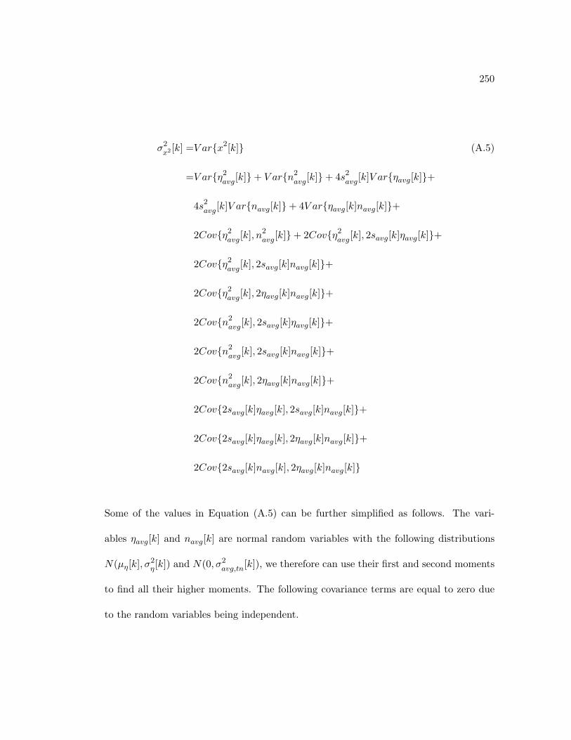
250
σ2x2 [k] =V ar{x2[k]} (A.5)
=V ar{η2avg
[k]}+ V ar{n2avg
[k]}+ 4s2avg
[k]V ar{ηavg[k]}+
4s2avg
[k]V ar{navg[k]}+ 4V ar{ηavg[k]navg[k]}+
2Cov{η2avg
[k], n2avg
[k]}+ 2Cov{η2avg
[k], 2savg[k]ηavg[k]}+
2Cov{η2avg
[k], 2savg[k]navg[k]}+
2Cov{η2avg
[k], 2ηavg[k]navg[k]}+
2Cov{n2avg
[k], 2savg[k]ηavg[k]}+
2Cov{n2avg
[k], 2savg[k]navg[k]}+
2Cov{n2avg
[k], 2ηavg[k]navg[k]}+
2Cov{2savg[k]ηavg[k], 2savg[k]navg[k]}+
2Cov{2savg[k]ηavg[k], 2ηavg[k]navg[k]}+
2Cov{2savg[k]navg[k], 2ηavg[k]navg[k]}
Some of the values in Equation (A.5) can be further simplified as follows. The vari-
ables ηavg[k] and navg[k] are normal random variables with the following distributions
N(µη[k], σ2η[k]) and N(0, σ2
avg,tn[k]), we therefore can use their first and second moments
to find all their higher moments. The following covariance terms are equal to zero due
to the random variables being independent.
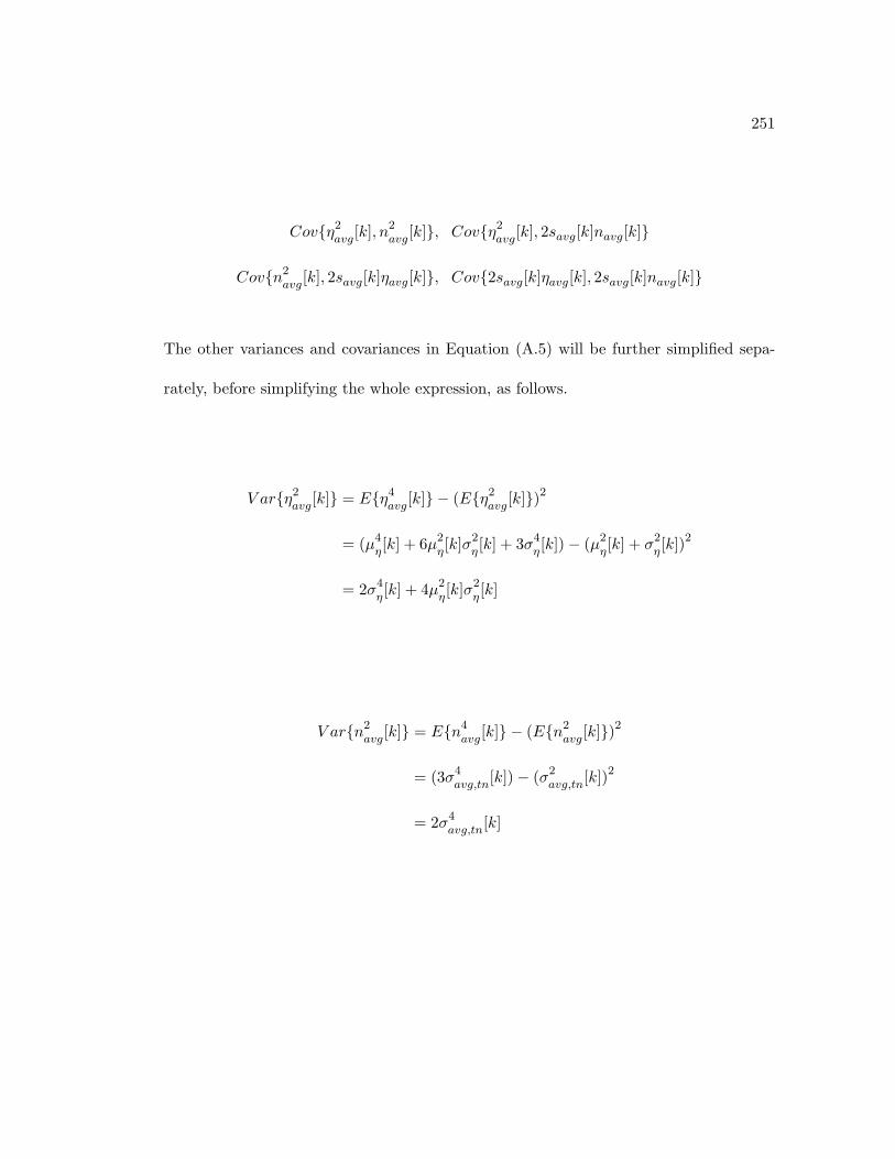
251
Cov{η2avg
[k], n2avg
[k]}, Cov{η2avg
[k], 2savg[k]navg[k]}
Cov{n2avg
[k], 2savg[k]ηavg[k]}, Cov{2savg[k]ηavg[k], 2savg[k]navg[k]}
The other variances and covariances in Equation (A.5) will be further simplified sepa-
rately, before simplifying the whole expression, as follows.
V ar{η2avg
[k]} = E{η4avg
[k]} − (E{η2avg
[k]})2
= (µ4η[k] + 6µ2
η[k]σ2
η[k] + 3σ4
η[k])− (µ2
η[k] + σ2
η[k])2
= 2σ4η[k] + 4µ2
η[k]σ2
η[k]
V ar{n2avg
[k]} = E{n4avg
[k]} − (E{n2avg
[k]})2
= (3σ4avg,tn
[k])− (σ2avg,tn
[k])2
= 2σ4avg,tn
[k]
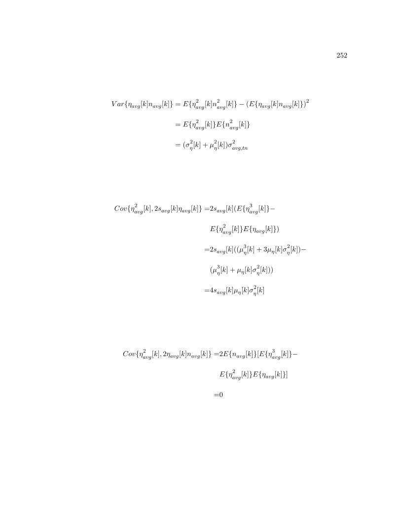
252
V ar{ηavg[k]navg[k]} = E{η2avg
[k]n2avg
[k]} − (E{ηavg[k]navg[k]})2
= E{η2avg
[k]}E{n2avg
[k]}
= (σ2η[k] + µ2
η[k])σ2
avg,tn
Cov{η2avg
[k], 2savg[k]ηavg[k]} =2savg[k](E{η3avg
[k]}−
E{η2avg
[k]}E{ηavg[k]})
=2savg[k]((µ3η[k] + 3µη[k]σ2
η[k])−
(µ3η[k] + µη[k]σ2
η[k]))
=4savg[k]µη[k]σ2η[k]
Cov{η2avg
[k], 2ηavg[k]navg[k]} =2E{navg[k]}[E{η3avg
[k]}−
E{η2avg
[k]}E{ηavg[k]}]
=0
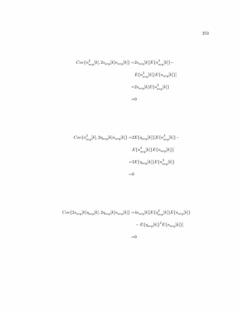
253
Cov{n2avg
[k], 2savg[k]navg[k]} =2savg[k][E{n3avg
[k]}−
E{n2avg
[k]}E{navg[k]}]
=2savg[k]E{n3avg
[k]}
=0
Cov{n2avg
[k], 2ηavg[k]navg[k]} =2E{ηavg[k]}[E{n3avg
[k]}−
E{n2avg
[k]}E{navg[k]}]
=2E{ηavg[k]}E{n3avg
[k]}
=0
Cov{2savg[k]ηavg[k], 2ηavg[k]navg[k]} =4savg[k][E{η2avg
[k]}E{navg[k]}
− E{ηavg[k]}2E{navg[k]}]
=0
254
Cov{2savg[k]navg[k], 2ηavg[k]navg[k]} =4savg[k][E{n2avg
[k]}E{ηavg[k]}
− E{navg[k]}2E{ηavg[k]}]
=4savg[k]σ2avg,tn
[k]µη[k]
Hence the Equation (A.5) can be simplified into the following,
σ2x2 [k] =(2σ4
η[k] + 4µ2
η[k]σ2
η[k]) + (2σ4
avg,tn[k]) + (4s2
avg[k]σ2
η[k])+ (A.6)
4s2avg
[k]σ2avg,tn
+ (4(σ2η[k] + µ2
η[k])σ2
avg,tn)+
8savg[k]µη[k]σ2η[k] + 8savg[k]σ2
avg,tn[k]µη[k]
The two expressions in Equations (A.6) and (A.4) represent the variance and the mean
respectively of the received signal squared for a certain value k. These two expressions
are functions of the first and second moments, µη[k] and σ2η[k] shown in Equations (A.2)
and (A.3), of ηavg[k]. Since µη[k] and σ2η[k] are functions of the random variable φ, so
is the mean and variance of squared received signal at k. The random variable φ is the
phase of the AM signal’s carrier which varies from experiment to experiment, therefore
the expected value of Equations (A.6) and (A.4) with respect to φ must be taken. Some
useful expected values with respect to φ follow,
255
E{µη[k]}φ = 0 E{µ2η[k]}φ = 0
E{σ2η[k]}φ =
A2η
2NeNm
σ2m
2E{σ4
η[k]}φ =
A4η
(2NeNm)2
3σ4m
8
E{µ2η[k]σ2
η[k]}φ = 0 E{µη[k]σ2
η[k]}φ = 0
Therefore the expected values of µx2 [k] and σ2x2 [k] with respect to φ are
E{µx2 [k]}φ = s2avg
[k] +A2η
2NeNm
σ2m
2+
σ2tn
2NeNm(A.7)
E{σ2x2 [k]}φ =
A4η
(2NeNm)2
3σ4m
4+ 2
σ4tn
(2NeNm)2 + (A.8)
4s2avg
[k]
(A2η
2NeNm
σ2m
2+
σ2tn
2NeNm
)+
4
(A2η
2NeNm
σ2m
2
)σ2tn
2NeNm.
Summing the expected values of the mean and variance, in Equations (A.7) and (A.8),
of the squared received signal over k = 0, 1, . . . , Ns−1, leads to the mean and variance of
the energy detector’s test statistic. The mean and variance of the distribution of the false
alarm is achieved by setting the QR signal in Equations (A.7) and (A.8) respectively to
zero.
256
µE,FA = Ns
(A2η
2NeNm
σ2m
2+
σ2tn
2NeNm
)
σ2E,FA
= Ns
(A4η
(2NeNm)2
3σ4m
4+
2σ4tn
(2NeNm)2
)
While the mean and variance of the distribution of the true positive is achieved by
summing the values in Equations (A.7) and (A.8) respectively over k = 0, 1, . . . , Ns − 1.
This leads to the following values,
µE,D = µE,FA + β2εs
σ2E,D
= σ2E,FA
+ 4β2εs
(A2η
2NeNm
σ2m
2+
σ2tn
2NeNm
)
257
Appendix B
Mean and Variance of Matched Filter Test Statistic,
in the Presence of AM and Thermal Noise
From section (4.2) the test statistic of the matched filter detector is of the following form
T (x, h) =N−1∑k=0
x[k] ∗ h[k],
the inner product of x[k] and h[k], where N = Nm ×Ns. This is a sum of independent
gaussian random variables, which is a gaussian random variable with a specific mean
and variance. To find the mean and variance of the test statistic, we first have to find
the mean and variance of the product x[k] ∗ h[k] for a specific value of k, under the
assumption that a QR signal exists within the received signal x[k], has the following
statistics,
E{x[k] ∗ h[k]} =β ∗ [Ae(−|−T/2+k∆|/T2∗) cos (∆ωr(−T/2 + k∆))]2+ (B.1)
h[k] ∗ (Aη2Ne
Ne∑i=1
[cos (∆ωAM (k∆ + (i− 1)τ) + φ)+
cos (∆ωAM (k∆ + (i− 1)τ + τd) + φ)])
258
V ar{x[k] ∗ h[k]} =h[k]2 ∗ (A2η
4N2e
Ne∑i=1
σ2m∗ (B.2)
[cos2 (∆ωAM (k∆ + (i− 1)τ) + φ)+
cos2 (∆ωAM (k∆ + (i− 1)τ + τd) + φ)] + σ2tn
)
where φ is a random variable that is uniformly distributed between −π and π. Taking
the expectation of the mean and variance of x[k]∗h[k] in Equations (B.1) and (B.2) with
respect to φ leads to the following statistics,
E{E{x[k] ∗ h[k]}}φ = β ∗ [Ae(−|−T/2+k∆|/T2∗) cos (∆ωr(−T/2 + k∆))]2 (B.3)
E{V ar{x[k] ∗ h[k]}}φ = h[k]2 ∗ (A2η
4Neσ2m
+ σ2tn
) (B.4)
Summing the expected values of the mean and variance, in Equations (B.3) and (B.4),
of the squared received signal over k = 0, 1, . . . , Nm × Ns − 1, leads to the mean and
variance of the matched filter’s test statistic. The mean and variance of the distribution
of the false alarm, achieved by setting the QR signal in Equations (B.3) and (B.4) to
zero and summing over k = 0, 1, . . . , Nm ×Ns − 1, are
µMF,FA = 0
259
σ2MF,FA
= ε ∗ (σ2AM
+ σ2tn
)
where σ2tn
and ε are defined in Equations (4.13) and (4.2) and σ2AM
is defined as
σ2AM
= (A2η/(4 ∗Ne)) ∗ σ
2m. (B.5)
On the other hand the mean and variance of the distribution of correct detection,
achieved by summing Equations (B.3) and (B.4) over k = 0, 1, . . . , Nm ×Ns − 1, are
µMF,D = β ∗ ε
σ2MF,D
= ε ∗ (σ2AM
+ σ2tn
)
where σ2tn
, σ2AM
and ε are defined in Equations (4.13) (B.5) and (4.2).
260
Appendix C
MATLAB Code
C.1 Data Generation Function
The following Matlab code was used to generate the simulated data used to test the
various algorithms.
%% m-file to simulate generation Sevaral QR and Noise Signals in SLSE Exp.
%% 11 April 2012
function [qr,qrtn,tn,qramtn,amtn]=sim_data_SD_BPWGAM(wstar,fo,T2star,T2eff,QR_amp,w_AM,AM_mag,AM_st,therm_std,Nm,Ne,Ns,fs,T_daq,b);
% Sample parameters
% wstar % QR frequency
% T2star % The decaying parameter
% T2eff % Decay of echoes across sequence
% QR_amp % 3.5 g Piperazine producses a 25 mV avg signal
% w_AM % location of AM carrier
% fo % Spectrometer offset frequency
261
% Pulse sequence and spectrometer parameters
% Nm % Length of modulation sequence
% Ne % Collect Ne echoes following each lock pulse (10)
% Ns % Number of samples per acquired spin echo
% fs % AD sample rateke
% Ts =1/fs % AD sample period
% T_daq = 1.738e-3; % Acutal Data Acquision window time
td = 100e-3; % time delay before lock pulse
t_save = 0; % time required to save a waveforem in seconds
%td = 100e-3; % time delay before lock pulse
%t_save = 11; % time required to save a waveforem in seconds
tau = 2e-3; % time between echoes
% Generating modulation sequence
b_cmp = bitcmp(b,1);
262
b_mod = reshape([b b_cmp]’,2*Nm,1);
ws = wstar;
wo = 2*pi*fo; % Frequency offset
% Centroid of baseband QR Signal
w_bb_QR = ws + wo - wstar;
Ns_am = round(Ns*(tau/T_daq)); % Number of samples used up by data
% acquisition window
Ns_d = round(Ns*(td/T_daq)); % Number of samples used by the
% time delay between sequences
Ns_save = round(Ns*(t_save/T_daq)); % Number of samples used by the
% save time between sequences
w_bb_AM = ws + wo - w_AM; % Centroid of AM spectra in baseband
263
% AM_mag*(1+m[k]), where m varies between -1 and 1, therefor max = 2*AM_mag
SNR = 20*log10(QR_amp/(AM_mag));
% time vector for each acquisition window
Ts = 1/fs;
ns = 1:Ns;
t_echo = (ns - Ns/2)*Ts;
t_am = linspace(0,T_daq,Ns);
% Initialize storage vectors for signal averaging
Nm = 2*Nm; % Generate twice the number of sequences for phase cycling
zv = zeros(Nm,Ns);
QR_seq = zv;
AM_tn1 = zv;
264
AM_tn2 = zv;
tn_001 = zv;
tn_002 = zv;
%% Design low pass Butterworth Filter
fc = 20e3; % 3 dB Cuttoff Frequency
%% Normalized, 1 corresponds to fs/2
wn = fc/(.5*fs); % Normalized Cuttoff Frequency
% Butter worth filter design
Ord = 8;
ftype = ’low’;
% Butter worth filter, Zero-Pole-Gain Design
[z, p, k] = butter(Ord,wn,ftype);
[sos,g] = zp2sos(z,p,k);
H = dfilt.df2sos(sos,g);
265
% % Plot and compare the results (As the order increases the transfer
% % function design can go unstable due to rounding errors)
%
% [H_mag,w_mag]=freqz(H,fs);
%
% % unwarp frequency
%
% w_mag = w_mag/(2*pi);
% w_mag = w_mag*fs;
%
% figure(1)
% semilogx(w_mag,20*log10(abs(H_mag)),’g’)
% ylim([-150 50])
% xlabel(’Frequency (Hz)’)
% ylabel(’Magnitude (dB)’)
% legend(’Pole Zero Gain Design’)
% title(’8th Order Butterworth Lowpass Filter Frequency Response’)
%% Design Bandpass Butterworth Filter
fs_CD = 44.1e3; % Sampling Frequency
fc1 = 40; % 3 dB Cuttoff Frequency left
266
fc2 = 1e4; % 3 dB Cuttoff Frequency right
%% Normalized, 1 corresponds to fs/2
wn1 = fc1/(.5*fs_CD); % Normalized Cuttoff Frequency left
wn2 = fc2/(.5*fs_CD); % NOrmailized Cutoff Frequency right
fn_bp = [fc1 fc2];
wn_bp = [wn1 wn2];
% Butterworth filter design
Ord_bp = 4;
ftype = ’bandpass’;
% Butterworth filter, Zero-Pole-Gain Design
[z_bp, p_bp, k_bp] = butter(Ord_bp,wn_bp,ftype);
[sos_bp,g_bp] = zp2sos(z_bp,p_bp,k_bp);
H_bp = dfilt.df2sos(sos_bp,g_bp);
% % Plot and compare the results (As the order increases the transfer
% % function design can go unstable due to rounding errors)
267
%
% [H_bp_mag,w_bp_mag]=freqz(H_bp,fs_CD);
%
% Unwarp frequency
%
% w_bp_mag = w_bp_mag/(2*pi);
% w_bp_mag = w_bp_mag*fs_CD;
%
% figure(1)
% semilogx(w_bp_mag,20*log10(abs(H_bp_mag)),’g’)
% ylim([-150 50])
% xlabel(’Frequency (Hz)’)
% ylabel(’Magnitude (dB)’)
% legend(’Pole Zero Gain Design’)
% title(’8th Order Butterworth Bandpass Filter Frequency Response’)
% Generating average vectors for QR Signal and RFI sources
% Initial time delays - used in calculating the AM carrier phase
time_delay_exp_1 = 0;
268
start_phase1 = 2*pi*rand-pi;
start_phase2 = 2*pi*rand-pi;
k_001 = ns;
t_sin = [-T_daq/2:Ts:T_daq/2];
t_sin = t_sin(1:Ns);
for km=1:Nm
for ke=1:Ne
% QR Signals, add the Ne decaying echoes into one row
QR_mag = exp(-abs(t_echo)/T2star);
QR_sig = QR_mag.*exp(i*(w_bb_QR*t_echo + b_mod(km)*pi));
269
QR_sig = filter(H,QR_sig);
QR_sig = ((QR_amp.*exp(-(ke-1)*tau/T2eff))/max(abs(real(QR_sig))))*QR_sig;
QR_seq(km,:) = QR_seq(km,:) + QR_sig;
% Amplitude Modulated Thermal noise of standard deviation
m1 = randn(1,Ns);
m1 = filter(H_bp,m1);
m1 = (AM_st/(((m1*m1’)/size(m1,2))^.5))*m1;
m2 = randn(1,Ns);
m2 = filter(H_bp,m2);
m2 = (AM_st/(((m2*m2’)/size(m2,2))^.5))*m2;
AMtn1 = (5+ m1).*cos(w_bb_AM*(t_am+time_delay_exp_1) - start_phase1);
270
AMtn1 = filter(H,AMtn1);
AMtn1 = (AM_mag/(((AMtn1*AMtn1’)/size(AMtn1,2))^.5))*AMtn1;
AMtn2 = (5+ m2).*cos(w_bb_AM*(t_am+time_delay_exp_1) - start_phase2);
AMtn2 = filter(H,AMtn2);
AMtn2 = (AM_mag/(((AMtn2*AMtn2’)/size(AMtn2,2))^.5))*AMtn2;
AM_tn1(km,:) = AM_tn1(km,:) + AMtn1;
AM_tn2(km,:) = AM_tn2(km,:) + AMtn2;
% Form complex thermal noise
therm_amp=therm_std;
tn_real1 = randn(1,Ns);
tn_real1 = filter(H,tn_real1);
tn_real1 = (therm_amp/(((tn_real1*tn_real1’)/size(tn_real1,2))^.5))*tn_real1;
271
tn_cmpl1 = randn(1,Ns);
tn_cmpl1 = filter(H,tn_cmpl1);
tn_cmpl1 = (therm_amp/(((tn_cmpl1*tn_cmpl1’)/size(tn_cmpl1,2))^.5))*tn_cmpl1;
tn1 = (tn_real1+i*tn_cmpl1);
tn_real2 = randn(1,Ns);
tn_real2 = filter(H,tn_real2);
tn_real2 = (therm_amp/(((tn_real2*tn_real2’)/size(tn_real2,2))^.5))*tn_real2;
tn_cmpl2 = randn(1,Ns);
tn_cmpl2 = filter(H,tn_cmpl2);
tn_cmpl2 = (therm_amp/(((tn_cmpl2*tn_cmpl2’)/size(tn_cmpl2,2))^.5))*tn_cmpl2;
tn2 = (tn_real2+i*tn_cmpl2);
272
% Thermal Noise different for sping echo
tn_001(km,:) = tn_001(km,:) + tn1;
tn_002(km,:) = tn_002(km,:) + tn2;
% Updating the time delay for the next echo
k_001 = k_001 + Ns_am;
time_delay_exp_1 = time_delay_exp_1 + tau;
end % End of one pulse train that produces Ne echoes
%time_delay_exp_1 = time_delay_exp_1 + td + ps_timing_jitter(kr+(km-1)*Nr,1);
time_delay_exp_1 = time_delay_exp_1 + td;
k_001 = k_001 + Ns_d;
273
% Adding the computer saving time + time_jitter random between 0 &
% 1 s if km is even, (i.e. after the an even number of pulses)
if(mod(km,2)==0)
% time jitter is a random between 0 and 1s when saving
%t_rand = rand;
% jitter is zero for no save time
% t_rand = tau*rand;
t_rand = 0;
%Even
time_delay_exp_1 = time_delay_exp_1 + t_save + t_rand;
k_001 = k_001 + Ns_save + ceil(Ns*(t_rand/T_daq));
end
end
274
%Perform phase cycling using the modulation sequence and its complement
qr_seq(:,:) = QR_seq(:,:);
qrtn_seq(:,:)= QR_seq(:,:) + tn_001(:,:);
tn_seq(:,:) = tn_002(:,:);
qramtn_seq(:,:)= QR_seq(:,:) + AM_tn1(:,:) + tn_001(:,:);
amtn_seq(:,:) = AM_tn2(:,:) + tn_002(:,:);
qr(:,:) = (qr_seq(1:2:Nm-1,:) - qr_seq(2:2:Nm,:))./(2*Ne);
qrtn(:,:) = (qrtn_seq(1:2:Nm-1,:) - qrtn_seq(2:2:Nm,:))./(2*Ne);
tn(:,:) = (tn_seq(1:2:Nm-1,:) - tn_seq(2:2:Nm,:))./(2*Ne);
qramtn(:,:) = (qramtn_seq(1:2:Nm-1,:) - qramtn_seq(2:2:Nm,:))./(2*Ne);
amtn(:,:) = (amtn_seq(1:2:Nm-1,:) - amtn_seq(2:2:Nm,:))./(2*Ne);
275
Bibliography
[1] Explosives - compositions, global security. http:///www.globalsecurity.org.
[2] Judge denies bail to accused shoe bomber. CNN, December 28 2001.
[3] Quantum magnetics inc. http://www.qm.com, August 2003.
[4] P. V. Czipott D. K. Lathrop Y. K. Lee E. E. Magnuson R. Mathews A. D. Hibbs,G. A. Barrall and S. A. Vierkotter. Landmine detection by nuclear quadrupoleresonance. In Abinash C. Dubey, James F. Harvey, and Thomas Broach, editors,,volume 3392:pages 522–532, 1998.
[5] J. L. Schiano A. J. Blauch and M. D. Ginsberg. Landmine detection using feedbackNQR. Detection and Remediation Technologies for Mines and Minelike Targets IV,volume 3710:pages 464–473, 1999.
[6] M. D. Rowe A. Jakobsson, M. Mossberg and J. A. Smith. Frequency selectivedetection of nuclear quadrupole resonance signals. IEEE Transactions on Geosicenceand Remote Sensing, 2005.
[7] M. D. Rowe A. Jakobsson, M. Mossberg and J. A. S. Smith. Exploiting tempera-ture dependency in the detection of NQR signals,. IEEE Transactaion on SignalProcessing, 2005.
[8] M. D. Rowe A. Jakobsson, M. Mossberg and J. A. S. Smith. Exploiting tempera-ture dependency in the detection of NQR signals. ICASSP, Detection, Estimation,Classification Theorgy and Applications, I:pp 653–656, 2005.
[9] J. B. Miller H. B. Suits A. D. Hibbs G. A. Barral R. Mathews A. N. Garroway, M.L. Buess and L. Barret. Remote sensing by nuclear quadrupole resonance. IEEETransactaion on Geoscience and Remote Sensing, Vol. 39(No. 6):pgs 1108–1118,2001.
[10] Luca Gammaitoni Adi. R. Bulsara, Mario E. Inchiosa and Frank E. Gordon.Stochastic resonance detector for weak signals. US Patent 6,008,642, Dec. 28, 1999.
[11] Bryan H. Suits Richard L. Garwin Allen N. Garroway, Joel B. Miller. Probe fordetecting a transient magnetic resonance signal, wherein the ratio of the Q of theprobe to the Q of the resonance signal is relatively large. US Patent 6,420,872 B1,Jul. 16, 2002.
[12] A. N. Garroway B. H. Suits and J. B. Miller. Noise-immune coil for unshieldedmagnetic resonance measurments. Jouranal of Magnetic Resonance, vol. 131:pp.154–158, 1998.
276
[13] A. N. Garroway B. H. Suits and J. B. Miller. Surface and gradiometer coils near aconducting body: The lift-off effect. Journal of Magnetic Resonance, vol. 135:pp.373–379, 1998.
[14] J. B. Miller B. H. Suits, A. N. Garroway and K. L. Sauer. 14N magnetic resonancefor materials detection in the field. Solid State Nuclear Magnetic Resonance, vol.24:pp. 123–136, 2003.
[15] A. J. Blauch. Modeling and Control Design in Nuclear Quadrupole Resonance:Application to Mind Detection and Interrogation. Ph.D. dissertation, PennsylvaniaState University, May 2000.
[16] C. R. Cahn. Performance of digital matched filter correlator with unknown inter-ference. IEEE Transactions On Communications, Com 19(No. 2):pgs 1163–1172,December 1971.
[17] G. A. Ciccarelli. Quadrupole Resonance Imaging with RF Magnetic Field Gradients.Honors thesis, Pennsylvania State University, May 2009.
[18] R. Resnick D. Halliday and J. Walker. Fundamentals of Physics. 6th Ed. Vol 5Wiley, New York, New York, 2001.
[19] T. P. Das and E. L. Hahn. Nuclear quadrupole resonance spectroscopy. Sold StatePhysics. Advances in Research and Applications, Supplemental 1., 1958.
[20] H. G. Dehmelt. Nuclear quadrupole resonance. American Journal of Physics, vol.42:pp. 110–120, 1953.
[21] R. R. Ernst. Sensitivity enhancement in magnetic resonance. i. analysis of themethod of time averaging. The Review of Scientific Instruments, Vol. 36(No. 12):pgs1689–1695, 1965.
[22] H. Xiong J. Li G. Liu, Y. Jiang and G. A. Barrall. Radio frequency interferencesuppression for landmine detection by quadrupoled resonance. EURASIP Jouranl onApplied Signal Processing: Special Issue on Radar Space-Time Adaptive Processing,In press.
[23] Lowell J. Burnett Geoffrey A. Barrall and Alan G. Sheldon. Method and system forcancellation of extranewous signals in nuclear quadrupole resonance spectroscopy.US Patent 6,392,408 B1, May 21, 2002.
[24] Geoffrey H. Goldman and Marc A. Ressler. Systems and methods for mine detection.US Patent 7,511,654 B1, Mar. 31, 2009.
[25] V. S. Grechishkin. NQR device for detecting plastic explosives, mines and drugs.Applied Physics, A 55:505–507, 1992.
[26] V. S. Grechishkin and N. Ya. Sinyavskii. New technologies: Nuclear quarupole reso-nance as an explosive and narcotic detection technique. Physics-Uspekhi, 40(4):393–406, 1997.
277
[27] D/ G. Griffiths. Introduction to Electrodynamics. Prentice Hall, Englewood, NewJersey, 1989.
[28] Monson H. Hayes. Statistical Digital Signal Processing and Modeling. John Wiley& Sons, Inc., 2009.
[29] T. Hirschfeld and S. M. Klainer. Short range remote NQR measurements. Journalof Molecular Structure, Vol 58:pgs 63–77, 1980.
[30] T. Hirschfeld and S. M. Klainer. Short range remote NQR measurements. Journalof Molecular Structure, 58:67–77, 1980.
[31] A. J. Blauch J. L. Schiano, T. Routhier and M. D. Ginsberg. Feedback optimizationof pulse width in the SORC sequence. Jouranl of Magnetic Resonance, 140:84–90,1999.
[32] R. J. Karpowicz and T. B. Brill. Librational motion of hexahydro-1,3,5-trinitro-s-triazine based on temperature dependence of the nitrogen-14 nuclear quadrupoleresonance spectra: The relationship to condensed-phase thermal decomposition.The Journal of Physical Chemistry, Volume 87, No. 12:pages 2109–2112, 1983.
[33] Kevi Krolicki and Jeremy Pelofsky. Nigerian charged for trying to blow up U.S. jet.Reuters, December 26 2009.
[34] A. N. Garroway M. L. Buess and J. B. Miller. NQR detection using a meanderlinesurface coil. Journal of Magnetic Resonance, Vol. 92(No. 2):pgs 348–362, 1991.
[35] A. N. Garroway M. L. Buess and J. B. Miller. Detection of explosives by nuclearquadrupole resonance. US Patent 5206592, 1993.
[36] R. A. Marino. Detection and identification of explosives by n NQR. In In Proceed-ings of New Concepts Symposium and Workshop on Detection and Identificationof Explosives, pages pages 399–403. New Concepts Symposium and Workshop onDetection and Identification of Explosives, 1978.
[37] A. B. Martinez and J. B. Thomas. Finite length discrete matched filters. Journal ofthe Franklin Institute, Pergamon Journals Ltd., Vol 321(No 5):251–260, May 1986.
[38] E. M. Purcell N. Bloembergen and R. V. Pound. Relaxation effects in nuclearmagnetic resonance absorption. Physical Review, Volume 73:pages 679–83, 1947.
[39] H. Negita. Line shape of 14N pure quadrupole resonance by the Zeeman modulation.The Journal of Chemical Physics, Vol. 44:pgs 1734–1740, 1966.
[40] J. E. Pacas. Measurement of the Effect of Different Transmitting and ReceivingOffset Frequencies in the SORC Pulse Sequence,. Honors thesis, Pennsylvania StateUniversity, May 2006.
[41] H. V. Poor. Robust matched fitlers. IEEE Trans. Inform. Theory, vol IT-29:pgs677–687, Sept. 1983.
278
[42] A. Michael Pusateri. Design of a quadrupole resonance probe using high-temperaturesuperconducting resonators. PhD thesis, The Pennsylvania State University, May2006.
[43] Fabrizio Dabbene Roberto Tempo, Giuseppe Calafiore. Randomized Algorithms forAnalysis and Control of Uncertain Systems. Springer-Verlag, 2004.
[44] M. D. Rowe and J. A. Smith. Mine detection by nuclear quadrupole resonance.Proceedings of the Eurel International Conference on the Detection of AbandonedLandmines, Vol. 431:pgs 62–66, 1996.
[45] K. Althoefer S. D. Somasundaram, J.A. Smith and L. D. Seneviratne. Detection oflandmines using nuclear quadrupole resonance (NQR): An overview. 2004.
[46] L. Carin I. Gorodnitsky A. D. Hibbs D. O. Walsh G. A. Barrall D. M. GregoryR. Mathews S. L. Tantum, L. M. Collins and S. A. Vierkotter. Signal processingNQR discrimination of buried landmines. in Proc. SPIE, vol. 3710:pp. 474–482,1999.
[47] J. R. P. Jayakody S. S. Kim and R. A. Marino. Experimental investigations ofthe strong off-resonant comb (SORC) pulse sequence in NQR. Zeitschrift Natur-forschung A: A Journal of Physical Sciences, Vol. 47(No. A):pgs 3709–3721, 1993.
[48] J. L. Schiano and M. D. Ginsberg. A pulsed spectrometer designed for feedbackNQR. XVth International Symposium on Nuclear Quadrupole Interactions, volume5a:pages 61–66, 1999.
[49] Jeffrey L. Schiano. Quadrupole resonance using narrowband probes and continuouswave excitation. US Patent 7511496, 2009.
[50] C. P. Slichter. Magnetic Relaxation. McGraw-Hill, New York, New York, July 2008.
[51] J. A. Smith. Mine detection by nuclear quadrupole resonance. Proc. Conf. DeminingTechnologies, pages pgs 314–321, 1998.
[52] J. A. S. Smith. Nuclear quadrupole resonance, general principles. Journal of Chem-istry Education, Vol. 48:pgs 39–49, 1971.
[53] J. A. S. Smith. Nitrogen-14 quadrupole resonance detection of RDX and HMX basedexplosives. European Convention on Security and Detection, Vol 408:pgs 288–292,May 1995.
[54] J. A. S. Smith and J. D. Shaw. Method of and apparatus for NQR testing selectednuclei with reduced dependence on a given environmental parameter. US Patent5583437, December, 1996.
[55] J. Stegenga. Humanitarian Demining: Detection algorithms for NQR signals. Mas-ter’s thesis, University of Twente (Netherland), January 2004.
[56] B. H. Suits. The noise immunity of gradiometer coils for 14N NQR land minedetection: Practical limitation. Applied Magnetic Resonance, 25:371–382, 2004.
279
[57] B. H. Suits and A. N. Garroway. Optimizing surface coils and the self-shieldedgradiometer. Journal of Applied Physics, vol. 94:pp. 4170–4178, 2003.
[58] V. T. Mikhaltsevich T. N. Rudakov and O. P. Selchikhin. The use of multi-pulsenuclear quadrupole resonance techniques for the detection of explosives containingRDX. Journal of Physics D: Applied Physics, vol. 30:pp 1377–1382, May 1997.
[59] Y. Tan. Advanced Signal Processing in Landmine Detection with Quadrupole Reso-nance. PhD thesis, Duke University, 2004.
[60] H. L. V. Trees. Detection, Estimation and Modulation Theory, Part IV, OptimumArray Processing. New York: John Wiley & Sons, Inc., 2002.
[61] G. L. Turin. Signal detection under noise interference in a game situation. IRETransactions Information Theory, IT-8(No. 2):pgs 347–557, September 1962.
[62] G. L. Turin. Minimax strategies for matched-filter detection. IEEE Transactionson Communications, Com 23(No. 2):pgs 1370–1371, November 1975.
[63] N. Ya. Sinyavskii V. S. Grechishkin and G. V. Mozzhukhin. A unilateral NQRexplosives detector. Russian Physics Jouranl, 35(7):635–637, 1993.
[64] B. Van Veen and K. Buckley. Beamforming: A versatile approach to spatial filtering.IEEE ASSP Magazine, vol. 5:pp. 4–24, April 1988.
[65] S. Verdu and H. V. Poor. On minimax robustness: A general approach and appli-cations. IEEE Transactions On Information Theory, IT-30(No. 2):328–340, March1984.
[66] S. Verdu and H. Vincent Poor. Minimax robust discrete-time matched filters. IEEETransactions On Communications, Com 31(No. 2):pgs 208–215, February 1983.
[67] J. Li Y. Jiang and P. Stoica. Array signal processing for QR. In The 36th AsilomarConference on Signals, Systems and Computers, pages pp. 893–897, Nov 2002.
[68] P. Stoica Y. Jiang and J. Li. Array signal processing in the known waveform andsteering vector case. IEEE Transactaion on Signal processing, vol. 52:pp 23–25,2004.
[69] S. L. Tantum Y. Tan and L. M. Collins. Landmine detection with nuclear quadrupoleresonance. in Proc. IGARSS’02, pages pp. 1575–1578, 2002.
[70] S. L. Tantum Y. Tan and L. M. Collins. Cramer-rao lower bound for estimatingquadrupole resonance signals in non-Gaussian noise. IEEE Signal Processing Letters,vol. 11:pp. 490–493, May 2004.
[71] S. L. Tantum Y. Tan and L. M. Collins. Kalman filtering for enhanced landminedetection using quadrupole resonance. IEEE Transaction on Geoscience and RemoteSensing, vol. 43:pp. 1507–1516, 2005.
Vita: Abdullah G. Almahri
Abdullah Ghazi Almahri, born on the 22nd of Janauary 1983, is the son of Ghazi Ab-
dulla Almahri and Khitam Yousef Maslamani. After completing his work at George C.
Marshall High School in Ankara, Turkey, he was sponsored by the UAE’s Ministry of
Higher Education to complete a Bachelor of Science in Electrical Engineering at The
Penn State University, University Park and completed his degree in December of 2004.
In 2005, Abdullah joined the Abu Dhabi National Oil Company. Shortly after that he
was granted a study leave to rejoin Penn State University to complete a Masters of
Science in Electrical Engineering, which he received in August of 2007. Abdullah then
resumed his studies at Penn State to pursue a Ph.D in Electrical Engineering.


![Photon Efficiency Limits in the Presence of Background Noise · background noise [3], which would imply the need to revert to radio frequency (RF) communication for very deep space](https://img.pdfslide.us/doc/110x75/5fb8e0c526155f25af49288f/photon-eficiency-limits-in-the-presence-of-background-noise-background-noise-3.jpg)