Embed Size (px)
Citation preview

Identification and Removal of Noise in Cardiac Signals
(CARDIO-NOISE)
Diogo Barreiro Nunes
MASTER’S DEGREE IN BIOMEDICAL ENGINEERING
Physics Department
Faculty of Sciences and Technology of University of Coimbra
February 2016


Identification and Removal of Noise in Cardiac Signals
(CARDIO-NOISE)
Author Supervisors
Diogo B. Nunes Professor Doutor César A. D. Teixeira
Professor Doutor Paulo F. P. de Carvalho
Dissertation presented to the Faculty of Sciences and Technology of the University
of Coimbra to obtain a Master’s degree in Biomedical Engineering
Coimbra, 2016


v
This thesis was developed in collaboration with:
Department of Computer Engineering
Center for Informatics and Systems of the University of Coimbra
WELCOME Project – Wearable Sensing and Smart Cloud
Computing for Integrated Care to COPD Patients with
Comorbidities
HeartSafe Project – Assessing Heart Function for Unsupervised
Homecare Applications through Multi-Channel Auscultation

vi

vii
Esta cópia da tese é fornecida na condição de que quem a consulta reconhece que os
direitos de autor são pertença do autor da tese e que nenhuma citação ou informação
obtida a partir dela pode ser publicada sem a referência apropriada.
This copy of the thesis has been supplied on condition that anyone who consults it is
understood to recognize that its copyright rests with its author and that no quotation
from the thesis and no information derived from it may be published without proper
acknowledgement.

viii

ix
Esta tese é dedicada à minha mãe e ao meu irmão,

x

xi
Acknowledgments
Gostaria de agradecer a várias pessoas pelo apoio, amizade e enriquecimento
académico que dispus ao longo desta fase da minha vida. Sem elas, não teria sido o
mesmo e eu não seria o mesmo.
Em primeiro lugar, agradeço ao Professor César Teixeira por ter fomentado em
mim uma postura crítica e autocrítica, estando sempre disponível para trocar ideias e
guiar-me da melhor forma. O mesmo se aplica ao Professor Paulo de Carvalho, que
sempre se mostrou disponível para partilhar o seu conhecimento e experiência.
Não poderia deixar de agradecer também aos Professores Jorge Henriques e Rui
Pedro Paiva pelas suas críticas construtivas e transmissão de conhecimentos ao longo da
tese. Tal como ao Departamento de Engenharia Informática (DEI) que me acolheu, aos
CISUC e aos projetos HeartSafe e WELCOME.
Por fim, agradeço aos amigos e familiares. À minha mãe e irmão que sempre me
transmitiram a sua confiança. Ao Carlos, Luís, Diana e Samuel que fizeram do DEI uma
segunda casa em Coimbra. Ao Jóni, André, Wilson, Joana, Carolina e Miguel pelo seu
apoio e amizade. Ao Rafael, Fábio, Gonçalo e Mafalda e restantes amigos por estarem
sempre presentes e fazerem de Coimbra uma experiência única. Finalmente, à minha
colega e amiga Adriana, que foi um alicerce e grande fonte de motivação ao longo de
toda a tese.

xii

xiii
Abstract
The increase of population ageing and sedentary lifestyle of today's society leads
to a greater demand for hospital services, which are unable to efficiently balance the
demand with the supply [1]. This problem led to the development of automatic systems
able to collect vital information from subjects on a daily basis, and through these, evaluate
possible pathologies without the need for patients to request hospital services, thus,
leading to a relief in demand and cost of medical consultations. These automatic systems
are called tele-monitoring systems, which are integrated with biosensors to acquire bio-
signals and computational algorithms to process them. These algorithms are
mathematical methodologies which provide the necessary intelligence to the system in
order to detect diseases and physiological information about a given subject. However,
due to the ambulatory nature of such systems, the acquisition of bio-signals is exposed
to numerous sources of noise, leading to the signals contamination. Noise can lead to
wrong event algorithm behavior, therefore, in order to prevent pathological false
detections it is essential to make the detection of contaminated periods. The focus of
this thesis is noise detection in bio-signals, particularly in Phonocardiogram (PCG) and
Electrocardiogram (ECG).
The noise detection methodology in the PCG context is characterized by being
a real-time and multi-channel process. It can be divided into two phases: a first phase
consists in searching a clean heart sound (HS) reference; the second phase compares
this reference with the remaining test windows and evaluates the presence of noise
based on the spectral similarity and the ratio of the total amount of high frequency
components, between the reference and test windows. In healthy signals the algorithm
achieved a sensitivity and specificity of 91.24% and 90.88%, respectively. In pathological
signals it reached a specificity of 91.68%. Its computational cost is 0.17s per minute of
PCG signal at 4000Hz. It was also compared on the same testing dataset with the
methodologies that presented the highest precision rates in literature, namely the
Modulation Filtering algorithm [2] and the Periodicity Based algorithm [3]. Additionally
to the better results presented by our algorithm, it was also more computationally
efficient than the compared methodologies.

xiv
The ECG noise detection methodology uses the Principal Component Analysis
(PCA) approximation error of each heartbeat and the presence of high frequency
components to evaluate the presence of noise in 4s periods in signals lasting at least 5
minutes. In the testing dataset it achieved 94.08% and 89.88% of sensitivity and specificity,
respectively, at critical SNR levels. Its computational cost is 0.14s per 5 minutes of ECG
sampled at 250 Hz. The highest documented precision in literature is 96.63% and 94.74%
of sensitivity and specificity, respectively, using an algorithm based on Empirical Mode
Decomposition (EMD) [4]. However, the authors only considered noise corruption in
the cases where the R-peaks were not recognizable, suggesting that the presented
precision is only valid for high degrees of noise. Additionally, our algorithm takes less
time to compute five minutes of ECG than the EMD algorithm takes to compute five
seconds.
Given the results, we believe that the developed methodologies fulfil the
proposed goals with high precision levels and low computational costs. It would be
interesting to see how the algorithms behave in real situations and uncontrolled
environments in order to assess its real use in tele-monitoring systems.

xv
Resumo
O envelhecimento da população e o estilo de vida sedentário da sociedade atual
resulta numa maior procura de serviços hospitalares, serviços esses incapazes de
balancear eficazmente a procura com a oferta [1]. Este problema levou a desenvolver
sistemas automáticos capazes de recolher informações vitais no dia-a-dia dos pacientes,
e através destas avaliar possíveis patologias, sem que os pacientes se deslocassem aos
serviços hospitalares, levando assim a um alívio na procura e custo de consultas médicas.
Estes sistemas automáticos são denominados de sistemas de tele-monitorização, onde
algoritmos computacionais são integrados em sistemas compostos por biossensores.
Estes algoritmos são metodologias matemáticas que dão ao sistema a inteligência
necessária para conseguir detetar patologias e informações fisiológicas sobre um
determinado sujeito. Porém, devido à natureza ambulatória destes sistemas, a aquisição
de bio sinais está sujeita a inúmeras fontes de ruído, levando à contaminação dos sinais.
A distorção dos sinais devido ao ruído pode levar os algoritmos de deteção de patologias
a detetar características patológicas quando elas não estão presentes, ou vice-versa. Por
isso é imprescindível que se faça a deteção dos períodos que estão contaminados, de
forma a não resultar em falsas deteções patológicas. Esta tese foca-se no âmbito da
deteção de ruído em bio sinais, nomeadamente, em Fonocardiograma (PCG) e
Eletrocardiograma (ECG).
A metodologia de deteção de ruído em PCG caracteriza-se por ser em tempo
real e multicanal. Pode ser dividida em 2 fases: uma primeira onde se procura uma
referência limpa de som cardíaco (HS); e uma segunda onde se compara essa referência
com as restantes janelas de teste e se avalia a presença de ruído com base na semelhança
espectral e a razão da soma dos componentes de altas frequências entre a referência e
as janelas de teste. A metodologia atingiu uma sensibilidade e especificidade de 91.24%
e 90.88%, respetivamente, em sinais saudáveis. Em sinais patológicos atingiu uma
especificidade de 91.68%. O seu custo computacional é de 0.17s por minuto de sinal
PCG a 4000Hz. A nossa abordagem foi também comparada com as metodologias que
apresentam a maior precisão na literatura, nomeadamente o algoritmo Modulation
Filtering [2] e o algoritmo Periodicity Based [3]. Para além de melhores resultados, a
nossa metodologia também apresentou uma maior eficiência computacional.
xvi
A metodologia de deteção de ruído em ECG utiliza o erro de aproximação por
Principal Component Analysis (PCA) de cada batimento cardíaco e a presença de
componentes de altas frequências para avaliar a presença de ruído em períodos de 4s
em sinais com duração de pelo menos 5 minutos. No dataset de teste atingiu 94.08% e
89.88% de sensibilidade e especificidade, respetivamente. O seu custo computacional é
de 0.14s por 5 minutos de ECG a 250 Hz. A maior precisão documentada na literatura
é de 96.63% e 94.74% de sensibilidade e especificidade, respetivamente, recorrendo a
um algoritmo baseado na Empirical Mode Decomposition (EMD) [4]. Porém, os autores
apenas consideram contaminação por ruído nos casos onde os picos R não são
reconhecíveis, sugerindo que a precisão documentada é apenas válida para altos níveis
de ruído. Para além disso, o nosso algoritmo leva menos tempo a processar 5 minutos
de ECG do que o algoritmo baseado em EMD leva a processar 5 segundos.
Dados os resultados, consideramos que as metodologias desenvolvidas cumprem
os objetivos, com altos valores de precisão e baixos custos computacionais. Seria
interessante ver como os algoritmos se comportam em situação real e em ambiente sem
controlo para poder avaliar o seu verdadeiro uso em sistemas de tele-monitorização.
xvii
List of Publications
D. Nunes, A. Leal, R. Couceiro, J. Henriques, L. Mendes, P. Carvalho, C.
Teixeira, "A low-complex multi-channel methodology for noise detection in
phonocardiogram signals," in Engineering in Medicine and Biology Society (EMBC), 2015 37th
Annual International Conference of the IEEE , vol., no., pp.5936-5939, 25-29 Aug. 2015
doi: 10.1109/EMBC.2015.7319743.
P. Carvalho, J. Henriques, C. Teixeira, R. Couceiro, T. Rocha, L. Mendes, D.
Nunes, I. Chouvarda, N. Maglaveras, R. Paiva, “Biodata Analytics for COPD,” submitted
in: 3rd International Conference on Biomedical and Heath Informatics (BHI), 24-27 February
2016.

xviii

xix
List of Figures
Figure 2.1 – Basic anatomy of the heart (extracted from [10]). .......................................................................... 3
Figure 2.2 – Cardiac nervous tissue (extracted from http://saintlukeshealthsystem.org)........................................... 5
Figure 2.3 – Main events in the cardiac cycle, and corresponding volume and pressure profiles (extracted
from [11]).............................................................................................................................................................................. 6
Figure 2.4 – Typical sound wave and spectrogram of a PCG signal. .................................................................. 7
Figure 2.5 – Auscultation sites (extracted from [11]). ........................................................................................... 9
Figure 2.6 – Spectrogram of a PCG signal contaminated by periods of physiological noise. ‘B’, ‘SW’ and
‘M’ corresponds to the artefacts originated by deep breathing, swallowing and body movement,
respectively. ........................................................................................................................................................................ 10
Figure 2.7 – Spectrogram of a PCG signal contaminated by periods of vocal noise. ‘S’, ‘C’ and ‘L’ and ‘O’
corresponds to the artefacts originated by speech, cough, laugh and other types, respectively. ................ 11
Figure 2.8 – Spectrogram of a PCG signal contaminated by periods of ambient noise. ‘D’, ‘OD’ and ‘MU’
and ‘P’ corresponds to the artefacts originated by door closing, object drop, music and phone ringing,
respectively. ........................................................................................................................................................................ 11
Figure 2.9 – Polarization waves of the cardiac events (extracted from [20]). ............................................... 14
Figure 2.10 – Einthoven triangle (extracted from [21]). ...................................................................................... 15
Figure 2.11 – ECG formation, Part1 (extracted from [22]). .............................................................................. 15
Figure 2.12 – ECG formation, Part2 (extracted from [22]). .............................................................................. 16
Figure 2.13 – The unipolar chest leads, or V leads (extracted from http://cvphysiology.com). ................ 17
Figure 2.14 – A normal 12-lead ECG (extracted from http: // pathology.wum.edu.pl)............................... 17
Figure 2.15 – The QRS Complex (extracted from http://studyblue.com). ..................................................... 18
Figure 2.16 – Spectral distribution of the different ECG waves. ....................................................................... 19
Figure 2.17 – The main noise types influence on the same ECG segment. .................................................... 19
Figure 2.18 – Spectral distribution of main noise types found in an ECG. ..................................................... 20

xx
Figure 2.19 – Magnitude of the spectral distribution of the signals contaminated with the different noise
types comparing to the clean ECG. ............................................................................................................................. 21
Figure 3.1 – Acquisition protocol, a) corresponds to the signal corrupted with ambient noise, b) signals
with the addition of physiological noise, and c) corresponds to signals induced with vocal noise. In some
acquisitions clean and noisy segments lasted for 20s, in others they lasted 10s. ............................................. 23
Figure 3.2 – Experimental setup. The arrows 1 and 2 are pointing to the microphones placed at the
pulmonary and mitral auscultation sites, respectively. ............................................................................................ 24
Figure 3.3 – Diagram of the multi-channel approach (MCA) noise detection algorithm in PCG. ............ 25
Figure 3.4 – Example of a 4s window divided in 1s segments. ........................................................................... 26
Figure 3.5 – Spectral distribution of the different 1s segments present in the 4s window. In this case we
have a spectral similarity of 0.9976. ............................................................................................................................. 28
Figure 3.6 – An example of a reference window. .................................................................................................. 29
Figure 3.7 – Algorithm’s noise detection result, and the respective reference and features result. The set
of parameters 𝑹𝒕𝒉, 𝑯𝑭𝒕𝒉 and 𝑭𝒄 were set to 0.92, 6.5 and 170, respectively. ............................................. 32
Figure 3.8 – ROC curves for the different parameter combinations in the training dataset. .................... 33
Figure 3.9 – Noise detection on a contaminated period (door closing). ........................................................ 35
Figure 3.10 – Differences between the different detection techniques. ......................................................... 36
Figure 4.1 – Segments of the noise records from Physionet used to add noise to the signals at different
SNR’s. EM corresponding to the electrode motion noise in the ‘em’ record of Physionet. MA
corresponding to the muscle noise in the ‘ma’ record. And BW corresponding to the baseline wandering
noise in the ‘bw’ record. ................................................................................................................................................. 43
Figure 4.2 – The effect that each noise type produces in a clean ECG segment at different SNRs. ........ 45
Figure 4.3 – Diagram of the noise detection algorithm in ECG. ....................................................................... 46
Figure 4.4 – Envelope computation of the ECG beats. ........................................................................................ 48
Figure 4.5 – Different amplitude beats, and the threshold variation. ............................................................... 48
Figure 4.6 – Plot of a lead-off period (1355s - 1361s). ......................................................................................... 50
Figure 4.7 – Illustration of how the beat matrix 𝑀 is computed. ..................................................................... 51
Figure 4.8 – Comparison between the approximation by PCA of a clean heartbeat and a noise corrupted
one. ....................................................................................................................................................................................... 52

xxi
Figure 4.9 – Result of the noise classification performed in an ECG signal with one noise corrupted
period. .................................................................................................................................................................................. 54

xxii

xxiii
List of Tables
Table 3.1 – Noise sensitivity (SS) and specificity (SP) for all the signals in training dataset. ....................... 33
Table 3.2 – Noise sensitivity (SS) and specificity (SP) for all the signals in the healthy testing dataset. Each
value of sensitivity and specificity, corresponds to mean value of the two runs for each subject and noisy
type. ...................................................................................................................................................................................... 37
Table 3.3 – Results corresponding to the signals acquired in the Mitral auscultation site for the different
single-channel algorithms, for each noise type. The Time row corresponds to the processing time in
seconds, each algorithm takes to analyze one minute of PCG signal with a sampling frequency of 4000Hz.
These results were computed using MATLAB version R2013b and a 4.00GHz Intel Core i7-4790k
processor. ........................................................................................................................................................................... 38
Table 3.4 – Results corresponding to the signals acquired in the Pulmonary auscultation site for the
different single-channel algorithms, for each noise type. ........................................................................................ 38
Table 3.5 – Results of sensitivity and specificity for each subject on the pathological dataset using the
multi-channel approach algorithm. ............................................................................................................................... 39
Table 3.6 – Results for each auscultation site, for the different single-channel algorithms in the
pathological dataset. ......................................................................................................................................................... 39
Table 4.1 – Results on the influence that different noise types have on the R-peak detector at different
SNR levels. These results were computed on the MLII test data. The results on the clean signals were
99.39% and 99.64% of sensitivity (SS) and specificity (SP), respectively. The average computational time
is 0.01s per minute of ECG signal. ................................................................................................................................ 55
Table 4.2 – Results on the influence that different noise types have on the Morphological Transform R-
peak detector at different SNR levels. These results were computed on the MLII test data. The results on
the clean signals were 99.19% and 99.99% of sensitivity and specificity, respectively. The average
computational time is 1.1s per minute of ECG signal. ............................................................................................ 55
Table 4.3 – Results of mean sensitivity and specificity on the testing data at different leads and SNR levels.
............................................................................................................................................................................................... 56
Table 4.4 – Results for each lead and noise type at critical SNR levels. .......................................................... 58

xxiv

xxv
Contents
Acknowledgments .................................................................................... xi
Abstract ................................................................................................... xiii
Resumo ..................................................................................................... xv
List of Publications ................................................................................. xvii
List of Figures .......................................................................................... xix
List of Tables ......................................................................................... xxiii
Contents ................................................................................................. xxv
Chapter 1 – Motivation and Objectives .................................................. 1
Chapter 2 – Background Concepts and State of the Art ...................... 3
2.1 Cardiac anatomy and physiology ................................................................. 3
2.2 The cardiac cycle and origin of the heart sounds (HS) .......................... 5
2.3 The cardiac cycle and the electrocardiogram (ECG) ........................... 13
Chapter 3 – Noise Detection in PCG signals ........................................ 23
3.1 Data acquisition ............................................................................................ 23
3.2 Methods .......................................................................................................... 24
3.3 Results ............................................................................................................. 32
3.4 Discussion ...................................................................................................... 39
3.5 Concluding remarks ..................................................................................... 41

xxvi
Chapter 4 – Noise Detection in ECG signals ........................................ 43
4.1 Data ................................................................................................................. 43
4.2 Methods .......................................................................................................... 46
4.3 Results ............................................................................................................. 55
4.4 Discussion ...................................................................................................... 57
4.5 Concluding remarks ..................................................................................... 59
Chapter 5 – Conclusion ........................................................................... 61
References ................................................................................................ 63
Appendix A ............................................................................................... 67
Appendix B ............................................................................................... 69

Chapter 1 – Motivation and Objectives
1
Chapter 1 – Motivation and Objectives
Cardiovascular diseases are the main cause of decease in Europe, being
responsible for 46% of the total mortality [5] and is estimated that costs €196 billion
per year to the EU economy [6]. Due to the increasingly population ageing, these costs
are predicted to grow, if no new strategies are adopted.
One of the strategies used to control the high demand of hospital services and
decrease the overall costs is the consideration of Telemedicine systems [7], where the
main objective is to move from a system centered in the Hospital to a system centered
on the Patient. Therefore, quality service is offered at a lower cost, where the access to
the specialized services is decentralized and the investment is made on a preventive clinic
rather than a curative clinic, with a higher participation from the patient.
The work developed in this thesis is in the context of one of the Telemedicine
areas, the Tele monitoring, where devices, like vests or beds with integrated sensors are
used to acquire bio-signals (e.g. electrocardiogram (ECG), phonocardiogram (PCG) or
Respiratory Lung Sounds (RLS)). Computational algorithms are then used to process
and analyze various physiological features and/or pathologies [8]. These apparatus are
also known as Personal Telehealth Systems, or just pHealth systems. However, due to
the ambulatory nature of such signal acquisition, it is expected that noise sources will
affect signals, changing the original information. The presence of noise artifacts is a
serious problem when the assessment of some pathologies is performed, since it may
distort the signal in a way that either hides, or mimics pathologic characteristics, leading
to misdiagnosis [9]. Therefore, a methodology that differentiates the signal from noise
artifacts is required, to prevent erroneous decisions when it comes to diagnosis.

Chapter 1 – Motivation and Objectives
2
The purpose of this work is therefore to develop noise detection algorithms for
the PCG and ECG signals. The particular choice of PCG and ECG signals is based on the
high mortality rate caused by cardiovascular diseases, thus so, being natural candidates
to integrate in tele monitoring systems. A low computational cost is sought in order to
make the algorithms feasible to be integrated in pHealth systems. The noise-
contaminated periods identified by the algorithms are then excluded from further
analysis, thus avoiding misdetection of pathologies. A noise detection strategy was
chosen in favor of a noise reduction/reconstruction one because there is a great amount
of available signal in the tele-monitoring context. Additionally, the noise reduction
approach may distort the original signal due to the filtering processes, hiding some
important features for diagnosis.

Chapter 2 – Background Concepts and State of the Art
3
Chapter 2 – Background Concepts and State of
the Art
2.1 Cardiac anatomy and physiology
The heart is responsible for pumping the blood through the entire body,
generating the driving force required for this vital task. It is divided in two sections, left
and right, separated by the septum, each side composed by an atrium and a ventricle
(see Figure 2.1). The right atrium receives the deoxygenated blood from the body and
pumps it to the right ventricle, which in turn pumps it to the lungs for oxygenation. The
arterial blood enters in the left atrium by the pulmonary veins, which passes it to the left
ventricle, which in turn pumps it to the entire body again. The atrioventricular valves
separate the atria and ventricles, namely the tricuspid valve on the right side and the
mitral valve on the left side. There is also the pulmonary valve that separates the right
ventricle and the pulmonary artery, and the aortic valve, that borders between the left
ventricle and aortic artery, collectively known as semilunar valves.
Figure 2.1 – Basic anatomy of the heart (extracted from [10]).

Chapter 2 – Background Concepts and State of the Art
4
The valves are responsible for directing the blood flow, not allowing an inversion
in blood circulation. The valves are formed by strong fibrous cords, named chordae
tendineae, which are connected to the cardiac epithelium. Depending on the pressure
profile existing on the different chambers, the valves will or will not allow the blood
flow.
The driving force is generated due the chambers contraction, which is regulated
by electrical impulses sent by the autonomous nervous system to the heart. The
electrical activity of the heart results in action potentials conducted by a specialized
nervous tissue and the cardiac muscle. The Electrocardiogram (ECG) measures the heart
electrical activity. A normal heartbeat is initiated in the sinoatrial (SA) node, which
receives an electrical stimulus from the autonomous nervous system to start a new
cardiac cycle. This stimulus is forwarded to the atrial muscle, which results in a
depolarization wave through the walls resulting in an atrial contraction, and to the
atrioventricular (AV) node. The AV node is the only transmission pathway from the SA
node to the ventricles in a healthy heart (see Figure 2.2). The only purpose of this AV
node is to delay the impulse conduction to the ventricles, giving enough time to the atria
to complete its contraction. After the atrial contraction, the electrical impulse is
conducted through the septum by the bundle of His which branches in right bundle branch
and left bundle branch ending in the Purkinje fibers, which are responsible for the
transmission of the electrical impulse to the ventricular muscle. When the ventricular
muscle is stimulated, the depolarization wave travels from the endocardium to the
epicardium, resulting in a ventricular contraction and in the consequent blood ejection
to the arteries.

Chapter 2 – Background Concepts and State of the Art
5
Figure 2.2 – Cardiac nervous tissue (extracted from http://saintlukeshealthsystem.org).
2.2 The cardiac cycle and origin of the heart sounds (HS)
The heart cycle is regulated by the electrical activity of the heart, regulating the
contraction of the atria and ventricles. It comprises two phases, systole and diastole.
Systole begins with the ventricular contraction, which increases the pressure inside the
ventricular lumen. Rapidly, the pressure inside the ventricles exceeds the atrial pressure,
resulting in the closure of the AV valves, originating the first heart sounds (HS), named
S1. After the closure of the AV valves, an isovolumetric contraction happens until the
ventricular pressure exceeds the pressure existing on the output arteries of the heart.
When the ventricular pressure is superior to the arteries pressure, the semilunar valves
open resulting in the blood ejection into the pulmonary and aortic arteries. The systole
ends when the pressure of the output arteries exceeds the ventricular pressure,
resulting in the closure of the semilunar valves and giving rise to the second HS, known
as S2. The closure of the valves ends the blood ejection into the arteries.
After the closure of the semilunar valves an isovolumetric relaxation occurs,
lowering the ventricular pressure. When the pressure inside the ventricles is lower than
in the atria, the AV valves open, allowing the entrance of blood to the ventricular lumen.
After that, an atria contraction happens, named atrial systole, which causes the remaining
blood present in the atria to enter into the ventricles. This phase of ventricular

Chapter 2 – Background Concepts and State of the Art
6
relaxation and filling, is named diastole. The process is repeated with the beginning of a
new systole.
Figure 2.3 – Main events in the cardiac cycle, and corresponding volume and pressure
profiles (extracted from [11]).
2.2.1 Phonocardiogram (PCG)
The phonocardiogram is a graphical representation of the HSs. This plot of the
sound waves allows the investigation of a wider extent of features than the auscultation
itself, thus being a highly efficient tool for diagnosis of some cardiac pathologies [12].
The phonocardiogram is obtained using microphones, which can be later represented
and processed. In Figure 2.4 is shown an example of a PCG segment in the temporal
and frequency domain.

Chapter 2 – Background Concepts and State of the Art
7
Figure 2.4 – Typical sound wave and spectrogram of a PCG signal.
2.2.2 Heart sound physiology
The HSs existing in the cardiac cycle are originated by the closure of the valves,
blood flow and vibrations of the heart muscle. Typically, there are four HSs in a cardiac
cycle. The first, S1, is clearly audible in the apical zone and in the fourth intercostal space
in the left side of the sternum. It is characterized by a large amplitude and time duration
when compared to the remaining HSs, having an average duration of 100-200ms.
Observing the spectral distributions of S1, it is possible to identify two prominent
frequency components in the 10-200Hz range. Although it is not consensual, the
evidence points that these two frequency components are due to the mitral and tricuspid
valve closure [11]. The properties of S1 are of great importance in the assessment of
cardiac pathologies. They reflect the functioning of the AV valves and the force of the
myocardium contraction. Another important characteristic of this HS is the temporal
delay between the closure of the tricuspid and mitral valve, which lasts in average 20-
30ms in a normal heart. If this time delay is much higher than normal, then is a strong
indicator of heart disease [11].
The second HS (S2) occurs in the beginning of diastole, and corresponds to the
closure of the semilunar valves. It is audible in the second and third intercostal space on
the left side of the sternum, and presents two main frequency components, which are
associated with the aortic and pulmonary arteries closure. Higher frequency

Chapter 2 – Background Concepts and State of the Art
8
components can be identified in the S2 spectrum, when comparing to S1. The second
HS also presents a temporal delay between the closures of the two semilunar valves, but
in this case, this delay is of greater duration. This is due to a higher pressure in the aortic
artery comparing to the existing one in the pulmonary artery, causing the aortic valve
to close before the pulmonary valve. The closing of the aortic and pulmonary valves are
two events typically heard during auscultation. The time delay between these two events
varies depending on the respiratory movements. In expiration, the duration of the delay
is less than 30ms, whereas in inspiration this delay is of greater duration being clearly
noticeable. The amplitude of the two components of S2 and the duration of the delay
between them, are valuable information for cardiac disease diagnosis [13].
The third HS (S3) is usually referred as gallop sound, such as the fourth HS (S4).
Both are low intensity and low frequency sounds, normally not audible in adults and
occur in the beginning and end of diastole, respectively. S3 has its origin in the vibrations
of the ventricular walls caused by the rapid inflow of blood into the ventricles. Its audition
is a sign of pathology, but is natural in children and young adults. In patients with mitral
regurgitation, the S3 is normally audible but don’t imply necessarily systolic dysfunction
or high ventricular pressure. In patients with aortic stenosis, S3 is less frequent [11].
S4 is caused by the ventricular walls distension when atria contraction happens.
Normally is not noticeable, but when it is, it is sign of reduced distensibility in one or
the two ventricles. The low ventricular distensibility causes the ventricular walls to make
abrupt movements when the atria contraction occurs, originating vibrations, which
produces the S4.
Certain HSs or heart features may be more perceptive in some areas of the
chest, therefore there are multiple auscultation sites, which are depicted in Figure 2.5.

Chapter 2 – Background Concepts and State of the Art
9
Figure 2.5 – Auscultation sites (extracted from [11]).
2.2.3 Pathological sounds
There are two main types of pathologies associated with valvular diseases and
detected in cardiac auscultation: the cardiac stenosis and cardiac insufficiency. The
stenosis is characterized by damage in the heart valves: where these valves lack the ability
to fully open. The blood is thereby forced to pass through the small opening at a higher
speed, causing a turbulent regime, and producing a sound. The valvular insufficiency or
regurgitation is characterized by the back flow of the blood, due to the incomplete
closure of the valves. Depending on the location of the heart valve deficiency, the
stenosis or insufficiency may be mitral, tricuspid, pulmonary or aortic.
The sounds associated with pathologies are called cardiac murmurs and are
originated by vibrations caused by turbulent blood flow in the cardiac structure. They
are normally noticeable in children and after physical exercise, without being correlated
with disease [11]. However, except for those cases, their presence may indicate stenosis
or insufficiency in the aortic, pulmonary or mitral valves. Information about the occurring
time and site they occur have great diagnosis value in cardiac diseases [11]. In addition
to the cardiac murmurs, the S3 and S4 may also be associated with pathologies as
mentioned before.

Chapter 2 – Background Concepts and State of the Art
10
Finally, innocent murmurs can also be heard not being however associated with
disease. Usually, they are cause by a high cardiac debit or by the reduction of the blood
viscosity.
2.2.4 Noise sources in PCG
Noise sources affecting PCG may have an external or internal origin. External
noise, or ambient, comprises any sounds which are produced in the environment where
the acquisition takes place, such as music, people talking in the background, a door
closing, and so on. The noise with an internal origin is all the noise produced inside the
subject’s body, such as speech, deep breathing, laughing and others. Typically, noise
artifacts are characterized by the presence of higher frequency components in the
spectrum than the existing ones in the clean PCG spectrum (see Figure 2.6, Figure
2.7 and Figure 2.8).
Figure 2.6 – Spectrogram of a PCG signal contaminated by periods of physiological noise. ‘B’,
‘SW’ and ‘M’ corresponds to the artefacts originated by deep breathing, swallowing and body
movement, respectively.

Chapter 2 – Background Concepts and State of the Art
11
Figure 2.7 – Spectrogram of a PCG signal contaminated by periods of vocal noise. ‘S’, ‘C’ and
‘L’ and ‘O’ corresponds to the artefacts originated by speech, cough, laugh and other types,
respectively.
Figure 2.8 – Spectrogram of a PCG signal contaminated by periods of ambient noise. ‘D’,
‘OD’ and ‘MU’ and ‘P’ corresponds to the artefacts originated by door closing, object drop, music and
phone ringing, respectively.
2.2.5 State of the art on noise detection and reduction in PCG
Some strategies were already proposed to detect noise-contaminated periods in
PCG signals.

Chapter 2 – Background Concepts and State of the Art
12
In [2], a framing of the signal is performed in three seconds windows, followed
by an evaluation of the stationarity in each window. This algorithm assumes the presence
of two components in PCG signals: a stationary and periodic component related with
respiratory sounds; and the quasi-stationary component related to HSs. The main goal
of the algorithm is the detection of interferences in the stationary component of the
signal, caused by transient noise sources. This is done by computing the short-time
Fourier transform (STFT), followed by filtering the temporal trajectories of each
frequency bin using a low-pass linear phase filter with a cut-off frequency of 1Hz, this
operation is coined as modulation filtering. Then, power ratios of differently sized sub
windows are extracted from the filtered temporal trajectories of each 3 second window.
Finally, classification of noise is done using a Support Vector Machine (SVM) classifier.
In [3] a bi-phase algorithm is presented. The first phase consist in the search for
a clean HS window that will be used as a template. In the second phase the found
template window will be compared with the remaining windows. The selection of the
reference window is based on periodicity signatures within a 4s window. The second
phase compares the spectral similarity and the maximum energy ratio between the
reference window and the remaining test windows to assess about the noise
contamination in the HS clips.
In [14] noisy periods are detected by feeding single layer perceptrons, which
were previously trained with clean and noisy data, with the wavelet coefficients of half
second windows of PCG. In another study [15], different heart cycles are segmented
resorting to an ECG gating. Afterwards, the mean correlation of the Spectral Power
Distributions of the different cycles is obtained in order to ascertain about the presence
of noise in a given PCG containing 10 heart cycles.
In [16] is also presented a methodology that uses the ECG gating to segment the
different heart cycles, but in this case, each heart cycle is divided in systole and diastole.
Each systole period is divided in two different segments the variance of each one is
computed. If the variance of one segment is superior to a given threshold, then, that
segment is classified as contaminated. Next, the systoles are divided in more segments
and if the standard deviation of each segment is lower than a given threshold, then that

Chapter 2 – Background Concepts and State of the Art
13
segments is considered noise free. Finally, the correlations between the systoles are
computed, and the ones with a higher correlation than 0.7 are considered noise free.
The same methodology is used in the diastole segments.
In addition to the above described methodologies in noise detection periods to
be posteriorly discarded, other noise reduction/cancelation methods have been
developed, namely in [17][18][19].
In [17] a speech enhancement method, based on the spectral domain minimum-
mean squared error (MMSE) estimation, is used to infer about presence of noise. In [18]
an extra microphone is used to record only interferences produced by external noise
sources, in order to perform noise subtraction to the signal containing the HSs. In [19]
the PCG is filtered in a defined band frequency in order to enhance the HS and reduce
the noise influence in the signal.
2.3 The cardiac cycle and the electrocardiogram (ECG)
The ECG consists in the recording of the action potentials in the heart. The
depolarization and repolarization waves are measured using a galvanometer, which is an
instrument that measures current. The type of wave, direction and intensity, determines
the ECG profile. A depolarization wave approaching the positive electrode will produce
a positive voltage, while moving away produces a negative voltage. The registered
amplitude is directly proportional to the muscle mass where the wave was produced.
For this reason, the waves originated in the ventricles present a higher amplitude due to
its higher muscle mass. Depending on the sensors location, it is possible to obtain
different perspectives from heart electrical activity. The different sensors configurations
are known as leads.

Chapter 2 – Background Concepts and State of the Art
14
2.3.1 ECG origin
Usually, there are four main waves registered in an ECG, each from a different
cardiac occurrence:
Figure 2.9 – Polarization waves of the cardiac events (extracted from [20]).
The depolarization waves do not travel in a straight line like depicted in Figure
2.9, instead they spread in all possible directions from the source point. However, the
vector sum of the wave results in a unique vector with the average direction and
intensity, named force vector. In Figure 2.9 it is depicted the frontal plane of the heart,
where the angles represent the different electrical axis for action potential measure. In
this plane, six different perspectives, or leads, are used to measurement: the standard
limb leads (I, II, e III, with the electrical axis situated in 0º, 60º, and 120º, respectively)
and the augmented limb leads (aVR, aVL, and aVF, with the electrical axis situated in -
150º, -30º, and 90º, respectively), in their whole named limb leads. These six leads can
also be represented in the Einthoven triangle depicted in Figure 2.10.
1. Depolarization wave corresponding
to the atrial contraction.
2. Depolarization wave from the
septum.
3. Depolarization wave from the
ventricular muscle tissue.
4. Repolarization wave from the
ventricular muscle tissue.

Chapter 2 – Background Concepts and State of the Art
15
Figure 2.10 – Einthoven triangle (extracted from [21]).
In the atrial depolarization the force vector has an electrical axis close to the 60º,
where the lead II axis is situated, so it is expected a positive voltage in the lead II, at this
positive deflection is called P wave. In lead III this deflection is almost unnoticeable
because the axis of this lead is almost perpendicular to the wave direction.
Figure 2.11 – ECG formation, Part1 (extracted from [22]).
The next depolarization wave is the one that occurs from the septum, with its
electrical axis near the 150º. As this wave is nearly perpendicular to the lead II axis, its

Chapter 2 – Background Concepts and State of the Art
16
influence in the respective ECG is diminished, presenting a small negative deflection,
since the projection of the force vector in the lead II axis is in the opposite way. In lead
I the influence of this depolarization is more noticeable, since the wave and lead direction
are close to each other, but of opposite ways, which reflects in a negative deflection. To
this negative deflection caused by the septum depolarization is given the name of Q
wave.
Figure 2.12 – ECG formation, Part2 (extracted from [22]).
Next, the depolarization wave travels through the apical zone with an axis close
to 60º, reflecting a positive deflection in the three standard limb leads called R wave.
The depolarization continues from the endocardium of the left ventricle to the
epicardium. Since the wave projection in the late stage of ventricular depolarization is
contrary to the lead III axis, there will be a negative deflection in voltage known as S
wave. In the end of the heart cycle occurs the ventricular repolarization, causing the T
wave.
In addition to the limb leads, there are more 6 leads which ‘look’ at the heart in
the transverse or horizontal plane in different perspectives, called V leads, presented in
Figure 2.13. The respective representations in the ECG depend on the electrical axis

Chapter 2 – Background Concepts and State of the Art
17
of each wave and on lead in the horizontal plane. The same principles of ECG formation
in the limb leads apply to the V leads.
Figure 2.13 – The unipolar chest leads, or V leads (extracted from http://cvphysiology.com).
A normal 12-lead ECG presents the following form.
Figure 2.14 – A normal 12-lead ECG (extracted from http: // pathology.wum.edu.pl).

Chapter 2 – Background Concepts and State of the Art
18
2.3.2 Typical ECG of one heart cycle
Figure 2.15 – The QRS Complex (extracted from http://studyblue.com).
P Wave: Wave resulted from the atrial depolarization. Its absence may
indicate a cardiac anomaly such as atrial fibrillation, while abnormally
large amplitude may indicate a greater amount of atrial muscle than
normal [20].
QRS Complex: Complex formed by the Q, R and S waves. As it is the
result of the ventricular depolarization, a greater mass is involved,
resulting in a greater amplitude. Abnormalities in this complex may
indicate severe anomalies [20].
T Wave: Wave resulted from the ventricular repolarization. Inversion
of the T wave with respect to the QRS complex and abnormal variations
in amplitude, frequency and symmetry of the waveform in some leads are
considered indicators of certain pathologies [20].

Chapter 2 – Background Concepts and State of the Art
19
Figure 2.16 – Spectral distribution of the different ECG waves.
2.3.3 Noise sources in ECG
There are three main noise sources in an ECG (see Figure 2.17):
Electrode Motion (EM).
Muscle Artifact (MA).
Baseline Wondering (BW).
Figure 2.17 – The main noise types influence on the same ECG segment.
0 10 20 30 40 50 600
0.2
0.4
0.6
0.8
1
Frequency (Hz)
Rela
tive P
ow
er
QRS Complex
P Wave
T Wave
ECG
a) Clean Segment b) EM Noise Corrupted
c) MA Noise Corrupted d) BW Noise Corrupted

Chapter 2 – Background Concepts and State of the Art
20
The EM noise is originated from the movement of the electrodes attached on
the body and is caused by body position changes, that leads to electrode-skin impedance
variations. This type of noise is considered the most troublesome since its frequency
spectrum overlaps with the spectrum of the QRS. Its presence may mimic some ectopic
beats and is difficult to be removed comparing to the other noise types [23],[24].
Muscle noise (MA) is caused by action potentials created by the muscles
surrounding the heart, with overlapping frequency components with the ECG signal.
This noise has also frequency components superior to the ones found in the clean ECG
[23],[24],[25].
The BW noise is characterized by oscillations of the ECG baseline, which are
usually caused by chest movements produced during breathing. It is characterized by low
frequencies, in the range of 0.1-1Hz [23],[24],[25].
Figure 2.18 – Spectral distribution of main noise types found in an ECG.
0 10 20 30 40 50 60 70 800
0.2
0.4
0.6
0.8
1
Frequency (Hz)
Rela
tive P
ow
er
EM
MA
BW

Chapter 2 – Background Concepts and State of the Art
21
Figure 2.19 – Magnitude of the spectral distribution of the signals contaminated with the
different noise types comparing to the clean ECG.
2.3.4 State of the art on noise detection and reduction in ECG
One of the strategies used to control the impact of artifacts consists in the
removal of noise periods when these are detected [4], [26]–[31].
In [31], before the separation of sources, the neguentropy (a gaussianity
measure), is used to evaluate the presence of noisy segments.
In [30], a morphological filtering is performed in order to extract the EMG from
the signals. As the influence of the QRS complexes is still present in the extracted vector,
a suppression of these peaks is performed by reducing the magnitude by one-tenth on
the corresponding periods. Finally, the detection of EMG noise presence is computed by
thresholding the result of the moving variance on the EMG extracted and QRS
suppressed vector. In [28] the use of accelerometers is explored in order to detect
movement artifacts caused by corporal position changes.
In [4], noise detection is performed by extracting statistical metrics, namely the
mean, variance and entropy, from the first Intrinsic Mode Function (IMF) obtained using
the Empirical Mode Decomposition (EMD).
0 20 40 60 80 100 120 140 160 180-70
-60
-50
-40
-30
-20
-10
Frequency (Hz)
Magnitude
Clean
EM
MA
BW

Chapter 2 – Background Concepts and State of the Art
22
In [29], statistical properties are explored using the Laplacian model of the ECG
signal. In [27], the Root Mean Square (RMS) error is calculated between the original
signal and the approximation resulted from the reconstruction by Principal Component
Analysis (PCA).
In [26], a set of detectors, each one being specific to a given type of noise, is
explored. The signal overall quality is weighted by the effects of each type interference.
Another strategy is the reduction/cancelation of noise in the ECG rather than
discarding the noisy periods [24], [31]–[33]. In [31], the Independent Component
Analysis (ICA) is used to separate the clean ECG signal from the noise sources. In [24],
denoising of ECG is performed resorting to a notch filter, and also to Wavelet and
Empirical Mode Decomposition (EMD) methods. In [32], adaptive filtering is used for
noise cancellation. In [33], a reduction of noise is performed by smoothing the signal
with a Savitzky-Golay filter.

Chapter 3 – Noise Detection in PCG signals
23
Chapter 3 – Noise Detection in PCG signals
In this chapter we are going to describe our low-complex and real-time
processing methodology in noise detection periods for posterior removal.
3.1 Data acquisition
Multi-channel acquisitions occurred in two distinct populations, using different
sensors and protocols. A detailed description is presented in the following subsections.
3.1.1 Healthy dataset
The PCG signals were acquired in a group of 23 healthy young subjects, that
agreed with data acquisition and processing under anonymous conditions. There is a
total of 370 minutes of PCG signals available for analysis. In order to evaluate the
detection capabilities of the algorithm, subjects had to follow a defined protocol involving
the deliberate/intentional production of noise during acquisitions. Three types of noise
were induced along the signals: ambient, physiological and vocal noise (see Figure 3.1).
For each subject we repeated two times the acquisition of one continuous signal for
each noise type, leading to the recording of a total of six PCGs per subject.
Figure 3.1 – Acquisition protocol, a) corresponds to the signal corrupted with ambient noise,
b) signals with the addition of physiological noise, and c) corresponds to signals induced with vocal
noise. In some acquisitions clean and noisy segments lasted for 20s, in others they lasted 10s.
Closing
Door
Object
Falling
Ambient
Music
Phone
Ringing
Breathing Swallowing
Muscle
MovementSpeaking Coughing
Laughing
(a)
(b)
(c)
0
Time (s)

Chapter 3 – Noise Detection in PCG signals
24
The PCG signals were recorded using the data logger Sensatron (Philips,
Eindhoven, Netherlands) with a sampling frequency of 4000Hz. The two microphones
were placed in the pulmonary and mitral auscultation sites, as presented in Figure 3.2.
Figure 3.2 – Experimental setup. The arrows 1 and 2 are pointing to the microphones
placed at the pulmonary and mitral auscultation sites, respectively.
3.1.2 Pathological dataset
These signals were acquired at the Coimbra University Hospital (HUC) from
only subjects with heart conditions. The dataset comprises of 8 signals acquired in 8
subjects, accumulating 12 minutes of PCG signals. The signals were acquired in an
uncontrolled hospital environment where noise is mainly originated due to abrasion of
the stethoscopes with the skin and external voices. Data were acquired recurring to
digital stethoscopes Meditron and by considering a sampling frequency of 2000 Hz. The
stethoscopes were placed at the tricuspid and pulmonary auscultation sites.
3.2 Methods
Two main goals were envisaged for the development of the algorithm. In first
place, it should be accurate and in second place it should be computationally efficient
and process data in real-time, enabling integration in tele-monitoring systems. A diagram
that generally depicts the algorithm is presented in Figure 3.3.

Chapter 3 – Noise Detection in PCG signals
25
Figure 3.3 – Diagram of the multi-channel approach (MCA) noise detection algorithm in
PCG.
The proposed algorithm can be divided in two phases: in the first phase there is
a search for a noise free window to be used as a template of a clean HS epoch; the
second phase uses the template as a reference window to compare with the test
windows, and assess about the presence of noise. The features chosen to compare test
and reference windows were based on spectral differences and greater amounts of high
frequency components in the contaminated segments (see Figure 2.6, Figure 2.7, and
Figure 2.8).

Chapter 3 – Noise Detection in PCG signals
26
3.2.1 Phase I
In the first phase, the two PCGs from both channels, are windowed in 4s frames
with an overlap of 70%. In each 4s window the two channels are summed and the
resulting mean is subtracted to the signal.
𝑆𝑊 = 𝑠𝑊𝑐ℎ𝑎𝑛𝑛𝑒𝑙1 + 𝑠𝑊
𝑐ℎ𝑎𝑛𝑛𝑒𝑙2 3.1
𝑆𝑊𝑑 = 𝑆𝑊 − 𝑚𝑒𝑎𝑛(𝑆𝑊) 3.2
In Equation 3.1, 𝒔𝑾𝒄𝒉𝒂𝒏𝒏𝒆𝒍𝟏 and 𝒔𝑾
𝒄𝒉𝒂𝒏𝒏𝒆𝒍𝟐 correspond to each channel signal in
each 4s window, and their summation is given by 𝑺𝑾. 𝑺𝑾𝒅 in Equation 3.2 corresponds
to the detrended 𝑺𝑾 signal in each window. To evaluate if a certain 4s window is a
proper candidate to look for a 1s reference window, the algorithm looks for a high
spectral similarity between different segments present in the window. So, we segment
the 4s window in 4 segments, each with 1s and no overlap, 𝑪𝒌 (see Figure 3.4).
Figure 3.4 – Example of a 4s window divided in 1s segments.
Now, with the different segments separated, we can calculate the spectral
similarity between them. This computation of spectral similarity was already used in [3]
and [15]. To obtain the spectral distribution of each 1s segment, we recur to the
0.5 1 1.5 2 2.5 3 3.5 4
-6000
-4000
-2000
0
2000
4000
6000
Sw
d
Time (s)
C3C
1C
2C
4

Chapter 3 – Noise Detection in PCG signals
27
Discrete Time Short-Time Fourier Transform (DTSTFT), Equation 3.3. The DTSTFT
divides the signal in time intervals, and in each one performs the Discrete Fourier
Transform (DFT). The final result is a matrix composed by the distribution of the
frequency components in each temporal trajectory.
𝐷𝑇𝑆𝑇𝐹𝑇[𝑚, 𝑘] = ∑ 𝑥[𝑛]𝑤[𝑛 − 𝑚]𝑒−2𝜋𝑖𝑘𝑛
𝑁−1
𝑛=1
3.3
In Equation 3.3, 𝑫𝑻𝑺𝑻𝑭𝑻[𝒎, 𝒌] is the DTSTFT of the signal 𝒙 with 𝑵 samples,
and 𝒘 is a window function. The 𝒌 variable corresponds to a specific frequency with a
total of 𝑲 frequency trajectories, 𝒎 to a time trajectory with a total of 𝑴 trajectories,
and 𝒏 to a sample of the signal.
We perform the DTSTFT of each 𝑪𝒌 using a Hanning window function with a
span of 8ms and 50% of overlap between consecutive windows. The spectral distribution
(𝑺𝑫𝒌) of 𝑪𝒌, given by Equation 3.4, is obtained by the summation of the 𝑫𝑻𝑺𝑻𝑭𝑻𝒌’s log
magnitude along the 𝑴 temporal trajectories and further calculation of the Root Mean
Square (RMS) of that sum (see Figure 3.5).
𝑆𝐷𝑘[𝑘] = √1
𝑀∑ (20𝑙𝑜𝑔10(|𝐷𝑇𝑆𝑇𝐹𝑇[𝑚, 𝑘] |))2
𝑀
𝑚=1
3.4
Recurring to the example of Figure 3.4, the spectral distributions of the
different segments are illustrated in Figure 3.5.

Chapter 3 – Noise Detection in PCG signals
28
Figure 3.5 – Spectral distribution of the different 1s segments present in the 4s window. In
this case we have a spectral similarity of 0.9976.
To measure the spectral similarity between the different segments, the Pearson
Correlation Coefficient, Equation 3.5, is computed for each pairwise 𝑺𝑫𝒌 combination.
𝐶𝑜𝑟𝑟𝑋𝑌 =𝑐𝑜𝑣(𝑋, 𝑌)
𝜎𝑋𝜎𝑌 3.5
In Equation 3.5, 𝒄𝒐𝒗 corresponds to the covariance of two variables, and 𝝈 the
standard deviation. If the average correlation is greater than 0.995, than it is assumed
that the 4s window is a proper candidate to find a clean reference window. If not, the
algorithm analyses the next 4s window with 70% of overlap. The value of 0.995 for
average correlation, was taken by using this methodology on the entire length of the
training signals, and assessing the noise sensitivity it provided to us. This value was able
to reach a noise sensitivity of 95%, in other words, it assures us a noise free 4s window
with 95% of certainty.
Next, if the condition of the clean 4s window is met, there is a search of a 1s
window to serve as a reference of a noise free window and compare it to the remaining
1s windows of the signal. The 1s reference window, 𝑹𝑬𝑭, is the one with the lowest
overall Teager-Kaiser Energy Operator (TKEO), Equation 3.8, present in the 4s window.
Once the TKEO increases when high amplitude and frequency sounds are present, the
0 200 400 600 800 1000 1200 1400 1600 1800 2000400
500
600
700
800
900
1000
1100
1200
Frequency (Hz)
Magnitude (
dB
)
SD
1
SD2
SD3
SD4
Chapter 3 – Noise Detection in PCG signals
29
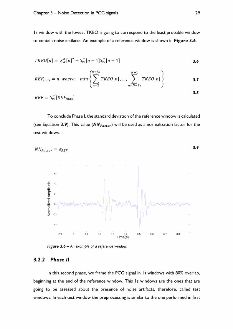
1s window with the lowest TKEO is going to correspond to the least probable window
to contain noise artifacts. An example of a reference window is shown in Figure 3.6.
𝑇𝐾𝐸𝑂[𝑛] = 𝑆𝑊𝑑 [𝑛]2 + 𝑆𝑊
𝑑 [𝑛 − 1]𝑆𝑊𝑑 [𝑛 + 1] 3.6
𝑅𝐸𝐹𝑖𝑛𝑑𝑠 = 𝑛 𝑤ℎ𝑒𝑟𝑒: 𝑚𝑖𝑛 { ∑ 𝑇𝐾𝐸𝑂[𝑛]
𝑛+𝑓𝑠
𝑛=2
, … , ∑ 𝑇𝐾𝐸𝑂[𝑛]
𝑁−1
𝑛=𝑁−𝑓𝑠
} 3.7
𝑅𝐸𝐹 = 𝑆𝑊𝑑 [𝑅𝐸𝐹𝑖𝑛𝑑𝑠]
3.8
To conclude Phase I, the standard deviation of the reference window is calculated
(see Equation 3.9). This value (𝑵𝑵𝑭𝒂𝒄𝒕𝒐𝒓) will be used as a normalization factor for the
test windows.
Figure 3.6 – An example of a reference window.
3.2.2 Phase II
In this second phase, we frame the PCG signal in 1s windows with 80% overlap,
beginning at the end of the reference window. This 1s windows are the ones that are
going to be assessed about the presence of noise artifacts, therefore, called test
windows. In each test window the preprocessing is similar to the one performed in first
2.9 3 3.1 3.2 3.3 3.4 3.5 3.6 3.7 3.8
-4
-2
0
2
4
6
Norm
aliz
ed A
mplit
ude
Time(s)
𝑁𝑁𝐹𝑎𝑐𝑡𝑜𝑟 = 𝜎𝑅𝐸𝐹 3.9

Chapter 3 – Noise Detection in PCG signals
30
phase, namely a summation of the two channels and the respective detrend (see Equation
3.1 and 3.2). After that, the test window and the reference window are normalized with
the 𝑵𝑵𝑭𝒂𝒄𝒕𝒐𝒓 obtained in the first phase. This 𝑵𝑵𝑭𝒂𝒄𝒕𝒐𝒓 is updated if the standard
deviation of the current test window is greater than the previous value.
In Equation 3.10, 𝑹𝑬𝑭𝒏𝒐𝒓𝒎 represents the reference window, 𝑹𝑬𝑭, normalized
by the 𝑵𝑵𝑭𝒂𝒄𝒕𝒐𝒓. In Equation 3.11, the test window, 𝑻𝑬𝑺𝑻 is computed by summing the
respective test windows in each channel, 𝒔𝒕𝒆𝒔𝒕𝒄𝒉𝒂𝒏𝒏𝒆𝒍𝟏 and 𝒔𝒕𝒆𝒔𝒕
𝒄𝒉𝒂𝒏𝒏𝒆𝒍𝟐, and removing the
respective mean. Finally, in Equation 3.12, 𝑻𝑬𝑺𝑻𝒏𝒐𝒓𝒎, results from the normalization of
the test window.
Finally, to ascertain about the presence of noise artifacts, two features are
computed, using the reference and test windows: the spectral similarity, 𝑹, and the High
Frequencies Power Spectral Density (HFPSD) ratio (𝑯𝑭𝒓𝒂𝒕𝒊𝒐).
In Equation 3.13, 𝑫𝑻𝑺𝑻𝑭𝑻𝑹𝑬𝑭𝒏𝒐𝒓𝒎 and 𝑺𝑫𝒓𝒆𝒇 correspond to the DTSTFT of the
reference window and its spectral distribution, respectively. While in Equation 3.14,
𝑅𝐸𝐹𝑛𝑜𝑟𝑚 =𝑅𝐸𝐹
𝑁𝑁𝐹𝑎𝑐𝑡𝑜𝑟 3.10
𝑇𝐸𝑆𝑇 = (𝑠𝑡𝑒𝑠𝑡𝑐ℎ𝑎𝑛𝑛𝑒𝑙1 + 𝑠𝑡𝑒𝑠𝑡
𝑐ℎ𝑎𝑛𝑛𝑒𝑙2) − 𝑚𝑒𝑎𝑛(𝑠𝑡𝑒𝑠𝑡𝑐ℎ𝑎𝑛𝑛𝑒𝑙1 + 𝑠𝑡𝑒𝑠𝑡
𝑐ℎ𝑎𝑛𝑛𝑒𝑙2) 3.11
𝑇𝐸𝑆𝑇𝑛𝑜𝑟𝑚 =𝑇𝐸𝑆𝑇
𝑁𝑁𝐹𝑎𝑐𝑡𝑜𝑟 3.12
𝑆𝐷𝑟𝑒𝑓[𝑘] = √1
𝑀∑ (20𝑙𝑜𝑔10(|𝐷𝑇𝑆𝑇𝐹𝑇𝑅𝐸𝐹𝑛𝑜𝑟𝑚[𝑚, 𝑘] |))2
𝑀
𝑚=1
3.13
𝑆𝐷𝑡𝑒𝑠𝑡[𝑘] = √1
𝑀∑ (20𝑙𝑜𝑔10(|𝐷𝑇𝑆𝑇𝐹𝑇𝑇𝐸𝑆𝑇𝑛𝑜𝑟𝑚[𝑚, 𝑘] |))2
𝑀
𝑚=1
3.14
𝑅 = 𝐶𝑜𝑟𝑟𝑆𝐷𝑡𝑒𝑠𝑡𝑆𝐷𝑟𝑒𝑓 3.15

Chapter 3 – Noise Detection in PCG signals
31
𝑫𝑻𝑺𝑻𝑭𝑻𝑻𝑬𝑺𝑻𝒏𝒐𝒓𝒎 and 𝑺𝑫𝒕𝒆𝒔𝒕 correspond to the DTSTFT of the test window and its
spectral distribution, respectively. The 𝑹 variable corresponds to the correlation
between the spectral distributions of the reference and test window, and is one of the
features to classify noise contaminated periods.
To calculate the second feature, the DFT (see Equation 3.16) is used to compute
the Power Spectral Density (PSD) of a given window (see Equation 3.17).
In Equation 3.16, 𝒘 corresponds to a Hamming window of the same size of the
signal window, with 𝑵 samples, and 𝒀𝒘 to the DFT of that signal segment. In Equation
3.17, 𝑷𝑺𝑫𝒘 is the PSD of a given window, with 𝒇𝒔 representing the sampling frequency.
To calculate the second feature we perform a summation along the 𝑷𝑺𝑫𝒘 at frequencies
higher than 𝑭𝒄 Hz, in order to obtain the total amount of high frequency components
of the reference and test windows (see Equation 3.18).
Now with the total amounts of high frequency components in the reference and
test windows (𝑯𝑭𝑷𝑺𝑫𝒘𝒓𝒆𝒇
and 𝑯𝑭𝑷𝑺𝑫𝒘𝒕𝒆𝒔𝒕, respectively) we calculate the ration
between them, 𝑯𝑭𝒓𝒂𝒕𝒊𝒐 in Equation 3.19. Having the two features computed we apply
a threshold technique to evaluate about the presence of noise contamination (see
Condition 3.20).
𝑌𝑤[𝑘] = ∑ 𝑥[𝑛]𝑤[𝑛]𝑒−2𝜋𝑖𝑘𝑛
𝑁−1
𝑛=1
3.16
𝑃𝑆𝐷𝑤[𝑘] =1
𝑓𝑠 ∙ 𝑁|𝑌𝑤[𝑘]|2 3.17
𝐻𝐹𝑃𝑆𝐷𝑤 = ∑ 𝑃𝑆𝐷𝑤[𝑘]
𝑁
𝑘=𝐹𝑐∙𝑁/(𝑓𝑠2
)
3.18
𝐻𝐹𝑟𝑎𝑡𝑖𝑜 =𝐻𝐹𝑃𝑆𝐷𝑤
𝑡𝑒𝑠𝑡
𝐻𝐹𝑃𝑆𝐷𝑤𝑟𝑒𝑓
3.19

Chapter 3 – Noise Detection in PCG signals
32
𝐼𝐹 𝑅 < 𝑅𝑡ℎ 𝑂𝑅 𝐻𝐹𝑟𝑎𝑡𝑖𝑜 > 𝐻𝐹𝑡ℎ → 𝑁𝑜𝑖𝑠𝑒 𝐶𝑜𝑛𝑡𝑎𝑚𝑖𝑛𝑎𝑡𝑖𝑜𝑛 3.20
In Condition 3.20, 𝑹𝒕𝒉 corresponds to threshold of the spectral similarity 𝑹, and
𝑯𝑭𝒕𝒉 to the threshold of 𝑯𝑭𝒓𝒂𝒕𝒊𝒐 feature.
Figure 3.7 – Algorithm’s noise detection result, and the respective reference and features
result. The set of parameters 𝑹𝒕𝒉, 𝑯𝑭𝒕𝒉 and 𝑭𝒄 were set to 0.92, 6.5 and 170, respectively.
3.3 Results
3.3.1 Tuning phase
To train the algorithm we used signals from six different subjects from the healthy
dataset, which has a total of 35 signals, sampled at 4000Hz. The best parameter
combination, namely 𝑹𝒕𝒉, 𝑯𝑭𝒕𝒉 and 𝑭𝒄, was found recurring to a Receiver Operating
Characteristic (ROC) analysis. The optimal combination was given by the highest module
of mean sensitivity and specificity on the training dataset. The best parameter
combination correspond to a mean sensitivity and specificity of 95.31% and 93.76% (see
Figure 3.8). The results for each subject and noise type are presented in Table 3.1.
0 20 40 60 80 100 120-5
0
5x 10
4
Sig
na
l
signal
detected
Reference
2.6 2.8 3 3.2 3.4 3.6 3.8-5000
0
5000
Re
fere
nce
0 20 40 60 80 100 1200.8
0.9
1
R
0 20 40 60 80 100 1200
10
20
30
HF
ratio
Time (s)

Chapter 3 – Noise Detection in PCG signals
33
Figure 3.8 – ROC curves for the different parameter combinations in the training dataset.
Table 3.1 – Noise sensitivity (SS) and specificity (SP) for all the signals in training dataset.
Noise Type
ID Age BMI
(Kg/m2) Run
Ambient Physiological Vocal
SS (%) SP (%) SS (%) SP (%) SS (%) SP (%)
1 35 28,01 1 99,13 91,11 100,00 86,75 98,57 93,79
2 97,82 96,17 87,92 89,85 99,94 91,79
2 28 22,47 1 97,86 99,12 90,90 89,44 99,93 97,54
2 93,16 100,00 89,56 90,65 99,74 98,35
3 33 25,11 1 100,00 91,39 97,35 93,04 - -
2 100,00 89,12 43,66 97,38 93,89 91,26
4 30 16,65 1 99,16 96,77 88,30 98,06 100,00 95,08
2 99,00 98,84 90,05 100,00 100,00 99,76
5 24 21,51 1 99,45 96,48 98,22 71,40 99,68 95,73
2 99,62 94,94 89,61 96,98 100,00 75,58
6 28 22,91 1 100,00 95,44 89,99 94,32 100,00 95,51
2 100,00 97,40 93,74 96,05 99,63 96,50
Average per Noise Type 98,77 95,57 88,27 91,99 99,22 93,72

Chapter 3 – Noise Detection in PCG signals
34
It is important to refer that the framing methodology that was used, in the
frontiers of noisy periods, is going to result in windows classified as noise where there
are both noise and clean samples. The algorithm was trained to not count as false
positives the clean samples present in a given window where both classes (clean and
noisy) of HSs are present. This was made in order to explore the full capabilities of the
algorithm on the noise detection. If we chose not to do this procedure, the lower
specificity due to the false positives present in a window with contaminated samples,
would result in an increase of the thresholds to compensate the low specificity and thus,
affecting our noise sensitivity. To conclude, we are imposing to the training methodology
that it is fine to classify a window as noise contaminated when this window has noise
periods. The results presented in Table 3.1 and Figure 3.8 are computed by having
this in account.
Although the algorithm has been trained to not count false positives in windows
where both classes (noisy and clean) are present, in a real situation these false positives
must be counted, as it discards clean periods, which might contain valuable information.
If we count the false positives at the margins of the noise periods, we get a mean
specificity of 85.88%, a drop of 7.88%. Although the decrease in specificity is not critical,
we have to take into account the entire length of the signal being analyzed. In the case
of the training dataset, the signals have a considerable high duration, comparing to the
assessment window duration, which results in a small drop of the specificity. However,
if we had signals with half the duration, this effect would be much more prominent, as
the false positives within a detected window would represent a higher percentage of the
signal - which is the case of the testing healthy dataset, where the different tasks have
only 10 seconds instead of 20 seconds of the training data. This problematic is shown
Figure 3.9.

Chapter 3 – Noise Detection in PCG signals
35
Figure 3.9 – Noise detection on a contaminated period (door closing).
This problem consists in a resolution problem of the framing methodology. We
could reduce the length of the analyzing 1s window, however it would result in a loss of
robustness, as it would most probably result in a reference window without at least one
HS cycle, and cause comparison problems between the reference and clean test
windows.
To overcome this resolution problem, maintaining the 1s window, the following
methodology is used. In each 1s window only the central 20% of the actual window
(which is renewed in each frame with 80% of overlap) is going to be classified as a noisy
or clean. A scheme that better describes this resolution narrowing is depicted in
Appendix A.
Recurring to the example of Figure 3.9 the result of the narrowing
methodology, or high resolution approach, is depicted in the following figure.
21 22 23 24 25 26 27
Time (s)
Signal
Detected Noise
Noise Contaminated Signal

Chapter 3 – Noise Detection in PCG signals
36
Figure 3.10 – Differences between the different detection techniques.
The results on the training dataset for the high resolution approach were 83.08%
and 95.72% of mean sensitivity and specificity, respectively. Although it resulted in a
trade-off of sensitivity for specificity, it provides us a higher independency regarding to
the signal duration. The decrease in sensitivity may be explained by the fact that some
large blocks of noise were annotated as one entire noise period, which increases the
count of false negatives due to the presence of small clean segments between the noisy
periods, as confirmed visually.
3.3.2 Testing phase
3.3.2.1 Healthy dataset
The healthy testing dataset comprises of 17 subjects, accounting for a total of 51
PCGs (six per subject) and has a total of 280 minutes of signal. The multi-channel
approach was tested using the set of parameters found in the training phase. The noise
sensitivity and specificity results for the testing dataset are presented in Table 3.2.
21 22 23 24 25 26 27
Time (s)
Signal
Detected Noise
Previous Detected Noise
Noise Contaminated Signal

Chapter 3 – Noise Detection in PCG signals
37
Table 3.2 – Noise sensitivity (SS) and specificity (SP) for all the signals in the healthy testing
dataset. Each value of sensitivity and specificity, corresponds to mean value of the two runs for each
subject and noisy type.
ID Age BMI
(Kg/m2) Sex
Ambient Physiological Vocal
SS (%) SP (%) SS (%) SP (%) SS (%) SP (%)
7 24 18,59 F 96,97 91,79 76,43 98,06 95,52 93,89
8 24 25,01 M 97,52 94,77 77,42 93,11 98,58 94,46
9 23 18,72 M 92,87 97,10 92,99 98,23 97,03 84,55
10 24 19,59 M 94,33 95,73 97,63 93,06 98,43 90,57
11 24 21,88 M 96,25 86,11 77,12 62,73 91,82 80,22
12 24 21,88 M 94,07 95,24 54,68 98,90 89,12 81,25
13 22 25,31 M 95,97 92,32 85,88 95,91 95,90 85,57
14 25 21,89 M 93,17 92,54 93,98 88,55 95,58 88,27
15 24 22,99 M 99,66 85,85 83,29 85,31 99,36 82,63
16 19 21,47 M 91,98 96,35 83,29 97,82 95,05 91,90
17 24 24,62 M 98,45 92,89 96,12 93,55 87,88 85,20
18 24 21,55 M 94,11 90,24 94,81 92,48 89,37 95,96
19 21 20,98 M 93,97 90,81 70,59 97,56 88,85 76,84
20 22 23,30 M 97,90 92,32 92,85 93,86 97,68 88,10
21 22 25,14 M 98,91 91,91 90,52 94,27 98,41 85,53
22 24 22,79 M 98,05 94,81 85,38 90,06 95,88 85,31
23 24 23,90 M 81,36 96,61 87,11 98,57 83,40 95,28
Average per Noise type 95,03 92,79 84,71 92,47 93,99 87,38
The multi-channel approach returns 91.24% and 90.88% of mean sensitivity and
specificity, respectively. We also tested this dataset for the signals downsampled to 2000
Hz, the results of the algorithm were 88.48% and 91.02% for mean sensitivity and
specificity, respectively.
The single channel approach (SCA) was also compared with other single-channel
methods, namely the Periodicity-based (PB) algorithm [3] and the Modulation Filtering
(MF) algorithm [2]. We have chosen these algorithms for comparison based on its
documented high precision and code availability. The results are presented in Table 3.3
and Table 3.4.

Chapter 3 – Noise Detection in PCG signals
38
Table 3.3 – Results corresponding to the signals acquired in the Mitral auscultation site for the
different single-channel algorithms, for each noise type. The Time row corresponds to the processing
time in seconds, each algorithm takes to analyze one minute of PCG signal with a sampling frequency
of 4000Hz. These results were computed using MATLAB version R2013b and a 4.00GHz Intel Core i7-
4790k processor.
Mitral SCA MF PB
SS (%) SP (%) SS (%) SP (%) SS (%) SP (%)
Ambient 93,64 94,00 84,92 52,46 97,10 89,13
Physiological 79,69 91,81 75,32 56,74 75,45 83,74
Vocal 86,22 92,56 96,26 47,28 86,54 75,09
Average 86,51 92,79 85,50 52,16 86,36 82,65
Time (s) 0,17 0,82 0,32
Table 3.4 – Results corresponding to the signals acquired in the Pulmonary auscultation site
for the different single-channel algorithms, for each noise type.
Pulmonary SCA MF PB
SS (%) SP (%) SS (%) SP (%) SS (%) SP (%)
Ambient 95,19 91,23 86,46 39,12 94,67 81,70
Physiological 81,10 90,04 73,49 41,48 79,55 77,25
Vocal 94,03 87,04 97,35 35,30 93,10 69,46
Average 90,11 89,43 85,77 38,63 89,11 76,14
3.3.2.2 Pathological dataset
We used the entire pathological dataset for test. The Multi-Channel Approach
results are presented in the following table.

Chapter 3 – Noise Detection in PCG signals
39
Table 3.5 – Results of sensitivity and specificity for each subject on the pathological dataset
using the multi-channel approach algorithm.
ID Age Sex BMI SS (%) SP (%) Condition
1 82 M 23,8 97,09 70,67 Cardiac Insufficiency Class 3; Ischemic
Cardiopathy
2 78 M 28,4 70,39 93,88 Cardiac Insufficiency Class 1; Valvular
disease; Coronary Disease
3 69 M 28,7 70,86 95,31 Cardiac Insufficiency Class 3; Mitral
Insufficiency
4 81 F 18,7 100,00 94,65 Cardiac Insufficiency
5 71 M 30,9 50,00 96,08 Cardiac Insufficiency Class 3; Coronary
Disease;
6 84 M 23,7 53,96 97,78 Cardiac Insufficiency; Ventricular
Dysrhythmia
7 82 M 23,7 76,09 97,59 Submitted to Aortic Arch Surgery
8 81 F 22,2 97,70 87,44 Cardiac Insufficiency Class 2;
Average 77,01 91,68
Comparison of the SCA algorithm with the other single-channel algorithms is
presented in Table 3.6.
Table 3.6 – Results for each auscultation site, for the different single-channel algorithms in the
pathological dataset.
Pulmonary Tricuspid
SS (%) SP (%) SS (%) SP (%)
SCA 88,20 87,20 84,30 90,86
PB 72,40 84,29 61,53 82,27
MF 79,68 55,80 81,51 48,29
3.4 Discussion
Looking at the results in Table 3.3, Table 3.4 and Table 3.6, it can be seen
that the SCA presents the highest mean sensitivity and specificity between all the
analyzed algorithms, as also the least computational time. The reason lies in its simplicity,
which provides the algorithm with robustness, generalization capabilities and low

Chapter 3 – Noise Detection in PCG signals
40
processing times. The physiological noise was the most difficult to detect among all the
tested algorithms, which can be due to the lower amplitudes and frequency components
this noise type presents.
A reason to justify the low specificity of the MF algorithm in the healthy and
pathological testing dataset, is the use of a 3s window to assess the noise periods, causing
a resolution problem. In the pathological dataset in addition to the resolution problem,
the MF algorithm may also have false detections due to the pathological HS, as referred
by the authors [2].
The PB algorithm presents a high sensitivity, however a lower specificity in
general, mainly due to resolution problems. The lower specificity in vocal noise,
comparing to the specificity in the signals with ambient and physiological noise, is due to
the differences in amplitude between the reference and the test windows, as some tasks,
e.g. coughing, laughing, may increase the heart rate, and result in the increase of energy
in the HS. As one of the features for noise classification in the PB algorithm is the energy
ratio between reference and test windows, this increase in heart rate, and consequently
its energy, may result in false detections.
The different methodologies were tested in pathological signals in order to infer
if the algorithms were sensitive to murmurs or other abnormal HSs. The high specificity
of the MCA and SCA indicates that the two approaches are able to differentiate between
pathological events from noisy periods.
The lower sensitivities in the pathological dataset compared to the ones in the
healthy dataset is due to the lower number of noisy periods along the signals, and thus,
not having a sufficient noise duration in each signal to infer with certainty about each
algorithm’s ability to detect noise. Other factor that influences the lower sensitivity is
that the acquisitions were made in a controlled and silent ambient, causing the
involuntary noise periods to have a low amplitude.
The results for the MCA and SCA prove the utility and efficacy of the developed
methodology. However, in a multi-channel situation, one may ask why not apply the
single-channel approach in each channel and join the final results, for a multi-channel

Chapter 3 – Noise Detection in PCG signals
41
resolution. In fact, the sum of the different channels is expected to result in an
amplification on the noise artifacts, as the noise sources will affect both channels. This
can be seen by the slightest better results of the MCA (see Table 3.2) comparing the
results of the SCA (see Table 3.3 and Table 3.4). Additionally, the computational time,
is reduced to half by using the MCA, an important asset to implement in tele-monitoring
systems.
The pathological dataset was acquired using two stethoscopes, each handled by
an individual subject, and the major noise source of this acquisitions was the abrasion
between the skin and stethoscopes, resulting on the independency of noise presence
between channels. Therefore, the usage of the SCA is a more suitable approach for this
situation, as we can compare by the results of the MCA and SCA, in Table 3.5 and
Table 3.6, respectively.
3.5 Concluding remarks
A fast and reliable algorithm has been developed, being suitable for integration in
real-time in a multi or single-channel acquisition system. Future work may include:
Increasing the number of subjects of the healthy and pathological testing
datasets in order to see the performance that the algorithm achieves in
a dataset that better depicts the overall population, and the diversity of
cardiovascular diseases;
Testing the methodology on signals that weren’t conditioned by any
acquisition protocol or a controlled environment, to inspect about its
performance in a real-life situation;
Assessment of the improvement in the detection of cardiac pathologies,
after the noisy periods detected by the MCA have been discarded from
further analysis.

Chapter 3 – Noise Detection in PCG signals
42

Chapter 4 – Noise Detection in ECG signals
43
Chapter 4 – Noise Detection in ECG signals
In this chapter we will describe an algorithm developed to detect noise periods
on single-lead ECG signals for quality evaluation. This algorithm had the finality to be
integrated in the WELCOME (http://www.welcome-project.eu) vest, a tele-monitoring
system, from the project of the same name. It was optimized to match the characteristics
of the referred system, namely, ECG signals at a sampling frequency of 250Hz, and 5
minutes of duration.
4.1 Data
We used the ECG signals available from Physionet (MIT-BIH Arrhythmia
Database - http://physionet.org/physiobank/database/mitdb), and noise records from the
MIT-BIH Noise Stress Database also from Physionet
(http://physionet.org/physiobank/database/nstdb/), all with a sampling frequency of
360Hz. The noise records were acquired in a way that the subject’s ECG signals were
not visible. Three types of noise were derived from these records, the baseline
wondering (BW), the electromyogram (EMG) artifact (MA), and the electrode motion
artifact (EM) (see Figure 4.1).
Figure 4.1 – Segments of the noise records from Physionet used to add noise to the signals
at different SNR’s. EM corresponding to the electrode motion noise in the ‘em’ record of Physionet. MA
corresponding to the muscle noise in the ‘ma’ record. And BW corresponding to the baseline
wandering noise in the ‘bw’ record.
0 2 4 6 8 10 12 14 16 18 20-500
0
500
EM
0 2 4 6 8 10 12 14 16 18 20-200
0
200
MA
0 2 4 6 8 10 12 14 16 18 20-400
-200
0
200
Time (s)
BW

Chapter 4 – Noise Detection in ECG signals
44
To add the noise to the ECG signals at different SNR’s, we used the ‘nst’ function
from the WFDB Software Package also provided by Physionet
(http://physionet.org/physiotools/wfdb.shtml), based on a peak to peak amplitude to
compute the gains to apply to the noise records.
The MIT-BIH Arrhythmia Database possess a total of 46 signals of lead MLII, 40
of V1, 4 of V2, 1 of V4, and 5 of V5, most of them with a high degree of arrhythmias
prevalence. We only used the signals with a high quality, i.e., the signals with few natural
noise periods. This selection was made to prevent the adverse effect of having noise
periods left to annotate, and thus, affecting the algorithm’s specificity, and also with the
objective of having a better insight about the algorithm capabilities on detecting different
noise types at different SNR’s, which we computationally added. So, we ended up with
a total of 25 signals of lead MLII (625 minutes), 21 of lead V1 (525 minutes), 4 of lead V2
(100 minutes), and 5 of lead V5 (125 minutes).
With the chosen dataset, we divided it in two subsets, one for training, and
another for test of the developed algorithm. We trained our algorithm on 6 different
signals of lead MLII, namely the records 201, 205, 213, 217, 223 and 231, comprising in
a total of 150 minutes. We have chosen these records due to its high quality signal and
the presence of various types of arrhythmias, in order to determine the parameters that
best discriminate the noise periods, keeping a low sensitivity to arrhythmia patterns.
The three noise types were added to the dataset at 6 different SNR levels, namely
-6, 0, 6, 12, 18 and 24 dB, like depicted in Figure 4.2.
To match the sampling frequency used in the WELCOME vest, all the signal were
down sampled to 250 Hz recurring to the Piecewise Cubic Hermite Interpolating
Polynomial (PCHIP).

Chapter 4 – Noise Detection in ECG signals
45
Figure 4.2 – The effect that each noise type produces in a clean ECG segment at different
SNRs.
24181260-6
SNR
(dB
)
Cle
an
EM
MA
BW
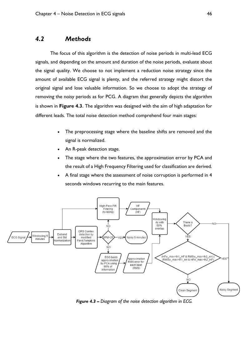
Chapter 4 – Noise Detection in ECG signals
46
4.2 Methods
The focus of this algorithm is the detection of noise periods in multi-lead ECG
signals, and depending on the amount and duration of the noise periods, evaluate about
the signal quality. We choose to not implement a reduction noise strategy since the
amount of available ECG signal is plenty, and the referred strategy might distort the
original signal and lose valuable information. So we choose to adopt the strategy of
removing the noisy periods as for PCG. A diagram that generally depicts the algorithm
is shown in Figure 4.3. The algorithm was designed with the aim of high adaptation for
different leads. The total noise detection method comprehend four main stages:
The preprocessing stage where the baseline shifts are removed and the
signal is normalized.
An R-peak detection stage.
The stage where the two features, the approximation error by PCA and
the result of a High Frequency Filtering used for classification are derived.
A final stage where the assessment of noise corruption is performed in 4
seconds windows recurring to the main features.
Figure 4.3 – Diagram of the noise detection algorithm in ECG.
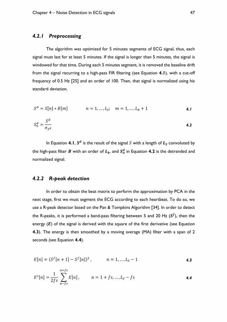
Chapter 4 – Noise Detection in ECG signals
47
4.2.1 Preprocessing
The algorithm was optimized for 5 minutes segments of ECG signal, thus, each
signal must last for at least 5 minutes. If the signal is longer than 5 minutes, the signal is
windowed for that time. During each 5 minutes segment, it is removed the baseline drift
from the signal recurring to a high-pass FIR filtering (see Equation 4.1), with a cut-off
frequency of 0.5 Hz [25] and an order of 100. Then, that signal is normalized using his
standard deviation.
𝑆𝑑 = 𝑆[𝑛] ∗ 𝐵[𝑚] 𝑛 = 1, … , 𝐿𝑆; 𝑚 = 1, … , 𝐿𝑏 + 1 4.1
𝑆𝑛𝑑 =
𝑆𝑑
𝜎𝑆𝑑 4.2
In Equation 4.1, 𝑺𝒅 is the result of the signal 𝑆 with a length of 𝑳𝑺 convoluted by
the high-pass filter 𝑩 with an order of 𝑳𝒃, and 𝑺𝒏𝒅 in Equation 4.2 is the detrended and
normalized signal.
4.2.2 R-peak detection
In order to obtain the beat matrix to perform the approximation by PCA in the
next stage, first we must segment the ECG according to each heartbeat. To do so, we
use a R-peak detector based on the Pan & Tompkins Algorithm [34]. In order to detect
the R-peaks, it is performed a band-pass filtering between 5 and 20 Hz (𝑺𝒇), then the
energy (𝑬) of the signal is derived with the square of the first derivative (see Equation
4.3). The energy is then smoothed by a moving average (MA) filter with a span of 2
seconds (see Equation 4.4).
𝐸[𝑛] = (𝑆𝑓[𝑛 + 1] − 𝑆𝑓[𝑛])2 , 𝑛 = 1, … , 𝐿𝑆 − 1 4.3
𝐸𝑠[𝑛] =1
2𝑓𝑠 ∑ 𝐸[𝑛]
𝑛+𝑓𝑠
𝑛−𝑓𝑠
, 𝑛 = 1 + 𝑓𝑠, … , 𝐿𝑆 − 𝑓𝑠 4.4

Chapter 4 – Noise Detection in ECG signals
48
Figure 4.4 – Envelope computation of the ECG beats.
The modification performed in this algorithm is in the threshold to assess the
peaks locations, which is adaptive. The threshold is derived by the result of a moving
average filter with a span of 2 seconds on the resulted energy vector. This modification
is made to take in account the individuality of each subject and lead, and on the different
possible beat amplitudes in the same signal, like depicted in Figure 4.5.
Figure 4.5 – Different amplitude beats, and the threshold variation.
The peaks location on each energy peak envelope are going to be the first sample
higher than the threshold. As the process of filtering causes a phase shift compared to
the initial signal, the real peak locations are assessed by finding the absolute maximum
14 16 18 20 22 24 26 28 30-5
0
5
10
Sn
d
14 16 18 20 22 24 26 28 30-5
0
5
Sf
14 16 18 20 22 24 26 28 300
0.2
0.4
Es
Time(s)
1680 1685 1690 1695 1700 1705 1710-4
-2
0
2
4
6
8
Sn
d
Signal
Detected Peaks
Normal Beat
PVC
1680 1685 1690 1695 1700 1705 17100
0.1
0.2
0.3
0.4
0.5
Es
Time(s)
Energy
Threshold
Peak Location
Minimum Threshold
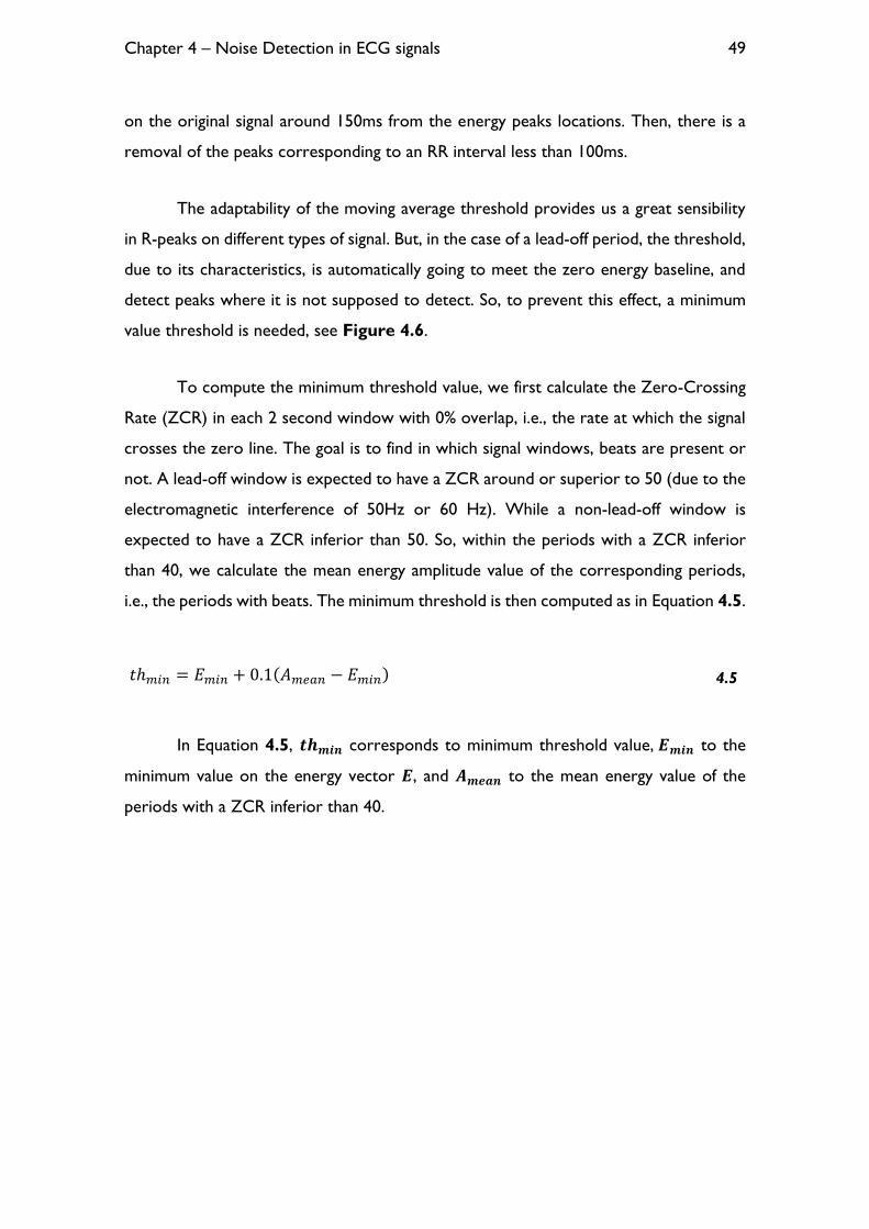
Chapter 4 – Noise Detection in ECG signals
49
on the original signal around 150ms from the energy peaks locations. Then, there is a
removal of the peaks corresponding to an RR interval less than 100ms.
The adaptability of the moving average threshold provides us a great sensibility
in R-peaks on different types of signal. But, in the case of a lead-off period, the threshold,
due to its characteristics, is automatically going to meet the zero energy baseline, and
detect peaks where it is not supposed to detect. So, to prevent this effect, a minimum
value threshold is needed, see Figure 4.6.
To compute the minimum threshold value, we first calculate the Zero-Crossing
Rate (ZCR) in each 2 second window with 0% overlap, i.e., the rate at which the signal
crosses the zero line. The goal is to find in which signal windows, beats are present or
not. A lead-off window is expected to have a ZCR around or superior to 50 (due to the
electromagnetic interference of 50Hz or 60 Hz). While a non-lead-off window is
expected to have a ZCR inferior than 50. So, within the periods with a ZCR inferior
than 40, we calculate the mean energy amplitude value of the corresponding periods,
i.e., the periods with beats. The minimum threshold is then computed as in Equation 4.5.
𝑡ℎ𝑚𝑖𝑛 = 𝐸𝑚𝑖𝑛 + 0.1(𝐴𝑚𝑒𝑎𝑛 − 𝐸𝑚𝑖𝑛) 4.5
In Equation 4.5, 𝒕𝒉𝒎𝒊𝒏 corresponds to minimum threshold value, 𝑬𝒎𝒊𝒏 to the
minimum value on the energy vector 𝑬, and 𝑨𝒎𝒆𝒂𝒏 to the mean energy value of the
periods with a ZCR inferior than 40.

Chapter 4 – Noise Detection in ECG signals
50
Figure 4.6 – Plot of a lead-off period (1355s - 1361s).
If the rate of beats per minute is less than 25, the whole 5 min are considered as
non-quality signal. This because the physiological impossibility of this heart rate, indicates
a disconnection of the electrodes from the skin.
4.2.3 Root mean square error of the approximation by PCA
The PCA will be performed on the beat matrix (𝑴), which consist in one beat
per line. Each beat 𝑩𝒊 in 𝑴 is obtained from the adjacent R-peaks locations of the current
R-peak location, 𝑹𝒊 (see Equation 4.6 and 4.7). As the lengths of each beat are different
we must perform a resampling to equalize all the beat lengths in order to perform the
PCA. The chosen length is 125 samples. All the beats in 𝑴 suffer a min-max
normalization (see Figure 4.7).
𝐵𝑖𝑟𝑒𝑎𝑐ℎ = 𝑚𝑖𝑛 {
𝑅𝑖 − 𝑅𝑖−1
2,𝑅𝑖+1 − 𝑅𝑖
2} 4.6
𝐵𝑖 = 𝑆𝑛𝑑[𝑘], 𝑘 = 𝑅𝑖 − 𝐵𝑖
𝑟𝑒𝑎𝑐ℎ, … , 𝑅𝑖 + 𝐵𝑖𝑟𝑒𝑎𝑐ℎ 4.7
1354 1356 1358 1360 1362 1364 1366 1368-4
-2
0
2
4
6
Sn
d
Signal
Detected Peaks
1354 1356 1358 1360 1362 1364 1366 13680
0.02
0.04
0.06
E
Time(s)
Energy
Threshold
Peak Location
Minimum Threshold

Chapter 4 – Noise Detection in ECG signals
51
Figure 4.7 – Illustration of how the beat matrix 𝑀 is computed.
Then we derive the eigenvalues and the eigenvectors of the covariance matrix of
𝑴, and make the reconstruction of the beats matrix based only on the eigenvectors that
provide at least 98% of the initial total variance. This value was found as the best to
discriminate between noise and clean periods according to a ROC analysis.
𝐴𝑝𝑝𝑟𝑜𝑥𝑀 = 𝑀𝑉𝑉𝑇 4.8
In Equation 4.8, the matrix 𝑨𝒑𝒑𝒓𝒐𝒙𝑴 is the result of the reconstruction of 𝑴
based only on the most significant eigenvectors, 𝑽. 𝑨𝒑𝒑𝒓𝒐𝒙𝑴 has the same size of 𝑴,
with 𝑵 lines and 125 columns, corresponding to the number of beats and the beat
lengths, respectively (see Figure 4.8).
......
Interpolation and Min-Max Normalization
Beat Matrix (M)

Chapter 4 – Noise Detection in ECG signals
52
𝑅𝑀𝑆𝑒𝑟𝑟[𝑖] = √∑ (𝐴𝑝𝑝𝑟𝑜𝑥𝑀[𝑖, 𝑗] − 𝑀[𝑖, 𝑗])2
𝑓𝑠/2
𝑗=1
, 𝑖 = 1, … , 𝑁; 𝑗 = 1, … , 𝑓𝑠/2 4.9
In Equation 4.9, the vector 𝑹𝑴𝑺𝒆𝒓𝒓 is the root mean square error between the
original beats and the approximation beats. This vector is one of the features used to
assess the presence of noise in ECG segments, [27]. Finally, is smoothed with a MA filter.
Figure 4.8 – Comparison between the approximation by PCA of a clean heartbeat and a
noise corrupted one.
4.2.4 High-pass FIR filtering
The second feature to assess the presence of noise artifacts is the result of a
high-pass FIR filter with a cut-off frequency (fc) of 90 Hz and an order of 100 (see
Equation 4.1). The fc of 90 Hz was found as the best to discriminate between noise and
clean periods according to a ROC analysis. Finally, this feature is smoothed with a MA
filter.
4.2.5 Noise assessment in 4s segments and thresholding
The assessment of corrupted periods is done by windowing the whole length of
the signal in 4 seconds chunks with 50% of overlap, and examine the two features in that
periods. Before the windowing, the thresholds must be determined to evaluate what is,
and what is not noise. These thresholds are not fixed to specific values, they change in
0 20 40 60 80 100 120 140-0.2
0
0.2
0.4
0.6
0.8
1
1.2
Sample
Clean Beat
Original Beat
Approximation Beat
0 20 40 60 80 100 120 140-0.8
-0.6
-0.4
-0.2
0
0.2
0.4
0.6
0.8
1
1.2
Sample
Noise Corrupted Beat
Original Beat
Approximation Beat

Chapter 4 – Noise Detection in ECG signals
53
each analyzed signal. To set them, we must first look for noise free periods. The clean
periods correspond to the 3 segments, each with 10 beats, with minimum 𝑹𝑴𝑺𝒆𝒓𝒓 and
no overlap. The average 𝑹𝑴𝑺𝒆𝒓𝒓 of these segments is taken as our reference error for
clean periods, 𝑹𝑬𝑭𝒆𝒓𝒓. The thresholds for the first feature are derived from this value
as shown in Equation 4.10 and 4.11.
𝑡ℎ1𝑒𝑟𝑟 = 𝑓1𝑒𝑟𝑟 ∙ 𝑅𝐸𝐹𝑒𝑟𝑟 4.10
𝑡ℎ2𝑒𝑟𝑟 = 𝑅𝐸𝐹𝑒𝑟𝑟 + 𝑓2𝑒𝑟𝑟 ∙ (𝑡ℎ1𝑒𝑟𝑟 − 𝑅𝐸𝐹𝑒𝑟𝑟) 4.11
In Equation 4.10 and 4.11, 𝒕𝒉𝟏𝒆𝒓𝒓 and 𝒕𝒉𝟐𝒆𝒓𝒓 correspond to the adaptive
thresholds for the first feature, 𝑹𝑴𝑺𝒆𝒓𝒓. The 𝒇𝟏𝒆𝒓𝒓 and 𝒇𝟐𝒆𝒓𝒓 are constant values found
in the training stage by ROC analysis and correspond to 2 and 0.5, respectively. To find
the thresholds for the second feature, 𝑯𝑭𝑿, a similar methodology is taken. The same
periods of time used to assess 𝑹𝑬𝑭𝒆𝒓𝒓 are used to calculate 𝑹𝑬𝑭𝑯𝑭, which is the mean
value of 𝑯𝑭𝑿 on those periods. The thresholds for the second feature are derived from
this value as shown in Equation 4.12 and 4.13.
𝑡ℎ1𝐻𝐹 = 𝑓1𝐻𝐹 ∙ 𝑅𝐸𝐹𝐻𝐹 4.12
𝑡ℎ2𝐻𝐹 = 𝑅𝐸𝐹𝐻𝐹 + 𝑓2𝐻𝐹 ∙ (𝑡ℎ1𝐻𝐹 − 𝑅𝐸𝐹𝐻𝐹) 4.13
The 𝒕𝒉𝟏𝑯𝑭 and 𝒕𝒉𝟐𝑯𝑭 correspond to the adaptive thresholds for the second
feature, 𝑯𝑭𝑿. The 𝒇𝟏𝑯𝑭 and 𝒇𝟐𝑯𝑭 are constant values found in the training stage by
ROC analysis and correspond to 1.115 and 0.6, respectively.
The reason to choose the 𝑹𝑴𝑺𝒆𝒓𝒓 feature to look for clean periods lies in his
highly sensitivity to noise. One might ask, why just not use this feature for classification
if it is so noise sensitive. The reason is that it is also sensitive for uncommon heart beat
types, which normally corresponds to abnormal heart beats and rhythms that we want
to diagnose. On the other hand, the 𝑯𝑭𝑿 feature don´t discriminate between different
heart beats or rhythm types, even if it hasn’t the noise sensitivity of the first. The
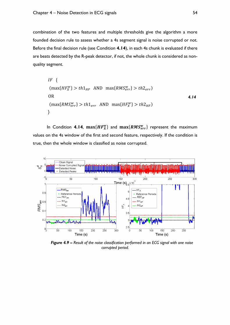
Chapter 4 – Noise Detection in ECG signals
54
combination of the two features and multiple thresholds give the algorithm a more
founded decision rule to assess whether a 4s segment signal is noise corrupted or not.
Before the final decision rule (see Condition 4.14), in each 4s chunk is evaluated if there
are beats detected by the R-peak detector, if not, the whole chunk is considered as non-
quality segment.
𝐼𝐹 {
(max{𝐻𝐹𝑋𝑤} > 𝑡ℎ1𝐻𝐹 AND max{𝑅𝑀𝑆𝑒𝑟𝑟
𝑤 } > 𝑡ℎ2𝑒𝑟𝑟)
OR
(max{𝑅𝑀𝑆𝑒𝑟𝑟𝑤 } > 𝑡ℎ1𝑒𝑟𝑟 AND max{𝐻𝐹𝑋
𝑤} > 𝑡ℎ2𝐻𝐹)
}
4.14
In Condition 4.14, 𝐦𝐚𝐱{𝑯𝑭𝑿𝒘} and 𝐦𝐚𝐱{𝑹𝑴𝑺𝒆𝒓𝒓
𝒘 } represent the maximum
values on the 4s window of the first and second feature, respectively. If the condition is
true, then the whole window is classified as noise corrupted.
Figure 4.9 – Result of the noise classification performed in an ECG signal with one noise
corrupted period.

Chapter 4 – Noise Detection in ECG signals
55
4.3 Results
All the results were computed using MATLAB version R2013b and a 4.00GHz
Intel Core i7-4790k processor. To see the influence that different noise types have on a
detection algorithm, we tested our R-peak detection algorithm on the contaminated
signals, see Table 4.1.
Table 4.1 – Results on the influence that different noise types have on the R-peak detector at
different SNR levels. These results were computed on the MLII test data. The results on the clean signals
were 99.39% and 99.64% of sensitivity (SS) and specificity (SP), respectively. The average computational
time is 0.01s per minute of ECG signal.
SNR
(dB)
EM MA BW
SS (%) SP (%) SS (%) SP (%) SS (%) SP (%)
-6 36,17 27,41 36,82 34,20 88,86 51,19
0 63,47 43,42 47,48 47,03 95,57 79,24
6 91,28 67,26 63,40 60,70 98,31 92,38
12 98,55 92,30 86,29 73,38 99,26 97,76
18 99,31 98,98 96,90 84,33 99,38 99,34
24 99,37 99,44 99,30 97,36 99,38 99,54
To see the noise influence on an algorithm independent to the our noise
detection algorithm, we tested the noise corrupted signals in another, more complex,
R-peak detection algorithm, based on morphological transform to segment the different
waves [35]. The result to sensitivity and specificity on the different noise contaminated
signals are presented in Table 4.2.
Table 4.2 – Results on the influence that different noise types have on the Morphological
Transform R-peak detector at different SNR levels. These results were computed on the MLII test data.
The results on the clean signals were 99.19% and 99.99% of sensitivity and specificity, respectively. The
average computational time is 1.1s per minute of ECG signal.
SNR
(dB)
EM MA BW
SS (%) SP (%) SS (%) SP (%) SS (%) SP (%)
-6 39,31 28,56 37,85 42,31 96,27 89,89
0 65,85 45,17 74,07 64,01 98,51 97,51
6 89,65 67,79 94,60 79,67 99,11 99,47
12 98,83 89,19 99,03 93,40 99,20 99,98
18 99,22 99,17 99,17 99,71 99,19 99,99
24 99,18 99,97 99,21 99,98 99,19 99,99

Chapter 4 – Noise Detection in ECG signals
56
In the following table (Table 4.3), are presented the algorithm’s results of
sensitivity and specificity on the testing data.
Table 4.3 – Results of mean sensitivity and specificity on the testing data at different leads
and SNR levels.
Lead SNR
(dB)
EM MA BW
SS (%) SP (%) SS (%) SP (%) SS (%) SP (%)
MLII
-6 99,06 88,32 99,54 89,25 99,84 88,59
0 99,27 89,04 99,60 89,26 99,61 88,59
6 99,47 89,92 99,58 89,19 96,07 88,98
12 98,92 90,37 98,44 90,37 75,85 91,39
18 89,47 91,96 94,79 91,60 48,13 94,46
24 63,05 92,73 82,17 92,14 26,17 95,38
V1
-6 99,42 87,73 99,73 87,71 99,50 88,25
0 99,51 88,88 99,74 88,25 99,61 88,91
6 99,19 89,04 99,58 88,25 96,62 88,17
12 94,95 89,33 98,49 89,89 89,82 89,38
18 77,53 89,79 94,24 89,93 55,28 92,74
24 38,69 91,63 76,49 91,15 34,92 95,40
V2
-6 97,40 88,77 97,83 88,49 97,54 86,43
0 97,75 89,47 98,12 88,54 97,73 87,64
6 97,85 89,92 98,00 87,82 98,03 89,73
12 96,81 90,33 98,07 88,48 92,22 89,80
18 89,48 92,27 95,08 90,39 56,41 95,27
24 55,04 94,61 82,18 93,68 33,45 95,61
V5
-6 96,55 90,42 100,00 88,47 99,74 89,58
0 98,61 90,33 100,00 88,47 98,86 89,88
6 97,78 90,76 99,01 88,70 91,71 92,29
12 89,96 92,59 96,34 90,38 67,26 94,34
18 70,91 93,90 88,39 93,51 34,51 96,09
24 33,09 95,25 60,19 95,75 10,14 96,10
Total Average 86,66 90,72 93,98 89,99 74,96 91,38
One big problem in trying to assess noise contaminated periods in an ECG signal
is that the algorithm may also detect abnormal heartbeats or rhythms as noise, and
misclassify certain periods that are of great value for diagnose. Thus so, is essential to
do a false positive analysis on the algorithm, and assess if the false positives are correlated
with abnormal heartbeats or rhythms. As the algorithm is dependent of the whole signal
being analyzed (due mainly to the 𝑹𝑴𝑺𝒆𝒓𝒓 feature which takes 98% of information of

Chapter 4 – Noise Detection in ECG signals
57
each signal) - and thus so, the algorithm’s response in the clean periods for the same
ECG may vary on the different noise types and SNR levels imposed – this false detection
rate is the mean value for all the signals at different SNR levels and noise types. As the
abnormal heartbeats have different manifestations on different leads, we did a false
positive analysis on each lead as shown in the tables in Appendix B.
The only alarming result in the false positive analysis is the 78.87% detection rate
on the supraventricular tachyarrhythmia rhythm in lead MLII. On the other hand, in the
whole test dataset we only possess 14 seconds of this rhythm type in the clean periods,
thus so, not having a sufficient statistical size to infer with certainty about the algorithm’s
sensitivity on this rhythm type.
4.4 Discussion
As we can see by the results of the two R-peak detector algorithms, the precision
of both are very similar on the clean signals, however, the Morphological Transform
(MT) based R-peak detector shows a slight higher robustness to noise compared to
ours. These noise robustness comes with a cost, as we can see by the computational
times. The computational cost of the MT algorithm is 2 orders of magnitude higher than
our R-peak detector. However, is important to refer that the MT algorithm is capable
of processing in real-time and besides the R-peaks detection, it also segments the P and
T waves, and the QRS complex.
One may think that using an R-peak detector that fails at high degrees of noise
on the segmentation of heartbeats is going to result in an adverse effect in the noise
sensitivity of the 𝑹𝑴𝑺𝒆𝒓𝒓 feature. However, it has the opposite effect on the noise
detection context, as a wrong segmentation is going to produce a segment that
completely differs from a typical heartbeat segment. As the PCA takes what is more
common, when taking 98% of the information, these segments that resulted from the
wrong segmentation, are going to have high approximation error, due to the nonsense
of the segmentation.

Chapter 4 – Noise Detection in ECG signals
58
This analysis on the R-peak detectors was with the intention to see the noise
influence at different SNR levels on a determined ECG detection algorithm. Based on
the results of Table 4.1 and Table 4.2, we consider that the noise influence is only
critical at [-6, 18] dB of SNR to the EM noise, [-6, 24] dB of to the MA noise, and [-6,
12] dB to the BW noise. The BW noise is less critical at higher SNR levels because this
noise influence is easily overcame with the detrend of the ECG signal, a feature that the
majority of ECG processing algorithms possess, and thus, being less troublesome [25].
The overall results to all leads were 94.08% and 89.88% of sensitivity and specificity,
respectively, in the range of the SNR levels we assumed critical, as presented in the
following table.
Table 4.4 – Results for each lead and noise type at critical SNR levels.
EM MA BW Average per
Lead [-6, 18] dB [-6, 24] dB [-6, 12] dB
SS (%) SP (%) SS (%) SP (%) SS (%) SP (%) SS (%) SP (%)
MLII 97,24 89,92 95,69 90,30 92,84 89,39 95,26 89,87
V1 94,12 88,95 94,71 89,20 96,39 88,68 95,07 88,94
V2 95,86 90,15 94,88 89,57 96,38 88,40 95,71 89,37
V5 90,76 91,60 90,66 90,88 89,39 91,52 90,27 91,33
Average per
Noise Type 94,49 90,16 93,98 89,99 93,75 89,50
94,08 89,88
TOTAL
The results in the table above show us a high sensitivity and specificity on noise
detection, and also that the precision of the algorithm does not vary much in different
leads, suggesting a good adaptability for the different leads, which we intended from the
beginning.
The highest precision documented in the literature is 96.63% and 94.74% of
sensitivity and specificity, respectively, on the ECG noise detection context [4].
However, the authors only consider noise corruption in the periods where the R-peaks
are not clearly recognizable, indicating that the documented precision is only
correspondent for noise corrupted signals at very low SNR levels. The computational
time of the referred algorithm is documented to be 0.2s per 5s of ECG signal at sampling
frequency of 180Hz using MATLAB 2010a on 2.66GHz Intel Core2 processor. The
computational time of our algorithm is 0.14s per 5 minute ECG signal with a sampling

Chapter 4 – Noise Detection in ECG signals
59
frequency of 250 Hz, this using MATLAB version R2013b and a 4.00GHz Intel Core i7-
4790k processor.
4.5 Concluding remarks
The noise detection algorithm in ECG demonstrates a high precision and a fast
performance, as well as a good adaptability for different leads and high specificity even
in pathological signals. The results indicate that it is a suitable algorithm to integrate in a
Tele-monitoring system.
It was already integrated in the WELCOME vest to discard 5 minutes signals
based on the amount of noise presence in the V2 lead, and also in the feature extraction
server (processing cloud) to detect noise periods in all the 12 leads before the detection
of Atrial Fibrillation is performed. We are waiting to see its performance in a real-life
situation and its behavior in the leads that weren’t analyzed, after the testing of the vest.

Chapter 4 – Noise Detection in ECG signals
60

Chapter 5 – Conclusion
61
Chapter 5 – Conclusion
Our main objective was the noise detection in bio-signals, namely on PCG and
ECG, recurring to fast and reliable noise detection algorithms.
In the PCG context we developed a high precision multi-channel (MCA)
algorithm capable of real-time processing, as a single-channel approach (SCA) of the
same. In comparison with the methodologies with the highest precision rates
documented in literature, our algorithm achieved the best results in the same testing
dataset, as also the best computational times. The MCA is suitable for integration when
the noise sources influence is simultaneously present in both channels. When the noise
influence is independent in each channel, the best integration would be the SCA,
although the MCA also achieves a good sensitivity, as we can see in the pathological
signals results in Table 3.5 and Table 3.6.
In the ECG context, the developed algorithm also presented high precision and
computational performance. In the ECG noise detection context, this analysis on various
leads, noise types, SNR levels, and false positive correlation with pathology, was the
most diverse analysis comparing to the ones found in literature. However, the ECG
algorithm is conditioned and optimized for the WELCOME project characteristics. It
would be interesting to develop a more general alternative algorithm without these
restraints, and hopefully capable to process in a real-time situation, which also explores
a multi-channel methodology. As soon as the WELCOME vest becomes available, we
could explore these new methodologies based on the 12-lead ECGs, as also assess the
performance of the developed single-channel algorithm in leads that weren’t tested.
Considering the final result, we think that we met the proposed goals. In a next
stage of the work, more bio-signals could be explored in the noise detection context, as
the Respiratory Lung Sounds or the Electrical Impedance Tomography, which are also
prone to noise contamination.

Chapter 5 – Conclusion
62

63
References
[1] J. R. Beard, A. Officer, I. A. de Carvalho, R. Sadana, A. M. Pot, J.-P. Michel, P.
Lloyd-Sherlock, J. E. Epping-Jordan, G. M. E. E. (Geeske) Peeters, W. R.
Mahanani, J. A. Thiyagarajan, and S. Chatterji, “The World report on ageing and
health: a policy framework for healthy ageing,” Lancet, Feb. 2016.
[2] J. P. Ramos, P. Carvalho, R. P. Paiva, and J. Henriques, “Modulation filtering for
noise detection in heart sound signals,” Proc. Annu. Int. Conf. IEEE Eng. Med. Biol.
Soc. EMBS, pp. 6013–6016, 2011.
[3] D. Kumar, P. Carvalho, M. Antunes, R. P. Paiva, and J. Henriques, “Noise
detection during heart sound recording using periodicity signatures.,” Physiol.
Meas., vol. 32, no. 5, pp. 599–618, 2011.
[4] J. Lee, D. D. McManus, S. Merchant, and K. H. Chon, “Automatic motion and
noise artifact detection in holter ECG data using empirical mode decomposition
and statistical approaches,” IEEE Trans. Biomed. Eng., vol. 59, no. 6, pp. 1499–
1506, 2012.
[5] M. Nichols, N. Townsend, P. Scarborough, and M. Rayner, “Cardiovascular
disease in Europe 2014: epidemiological update,” Eur. Heart J., vol. 35, no. 42, pp.
2950–2959, 2014.
[6] Nichols Melanie, T. Nick, S. Peter, and R. Mike, European Cardiovascular Disease
Statistics, no. September Issue. 2012.
[7] A. C. Norris, “Scope, Benefits and Limitations of Telemedicine,” in Essentials of
Telemedicine and Telecare, John Wiley & Sons, Ltd, 2001, pp. 19–38.
[8] C. U. Lehmann, E. Ammenwerth, and C. Nohr, Studies in Health Technology and
Informatics. 2013.
[9] J. G. F. Cleland, A. A. Louis, A. S. Rigby, U. Janssens, and A. H. M. M. Balk,
“Noninvasive Home Telemonitoring for Patients With Heart Failure at High
Risk of Recurrent Admission and Death,” J. Am. Coll. Cardiol., vol. 45, no. 10, pp.
1654–1664, 2005.
[10] C. M. Lewandowski, N. Co-investigator, and C. M. Lewandowski, “Inquiry into
Life,” Eff. Br. mindfulness Interv. acute pain Exp. An Exam. Individ. Differ., vol. 1, pp.
1689–1699, 2015.
[11] A. K. Abbas and R. Bassam, Phonocardiography Signal Processing, vol. 4. 2009.

64
[12] R. L. Watrous, “Computer-aided auscultation of the heart: From anatomy and
physiology to diagnostic decision support,” Annu. Int. Conf. IEEE Eng. Med. Biol. -
Proc., pp. 140–143, 2006.
[13] P. P-E, Textbook in medical physiology and pathophysiology - essentials and clinical
problems. 2000.
[14] S. Rajan, R. Doraiswami, R. Stevenson, and R. Watrous, “Wavelet based bank of
correlators approach for phonocardiogram signal classification,” Proc. IEEE-SP Int.
Symp. Time-Frequency Time-Scale Anal. (Cat. No.98TH8380), pp. 77–80, 1998.
[15] P. Carvalho, P. Gilt, J. Henriques, L. Eugenio, and M. Antunes, “Low complexity
algorithm for heart sound segmentation using the variance fractal dimension,”
IEEE Int. Work. Intell. Signal Process. 2005., pp. 194–199, 2005.
[16] D. Barschdorff, U. Femmer, and E. Trowitzsch, “Automatic phonocardiogram signal analysis in infants based on wavelet transforms and artificial neural
networks,” Comput. Cardiol. 1995, pp. 753–756, 1995.
[17] A. S. Paul, E. a Wan, and A. T. Nelson, “Noise reduction for heart sounds using
a modified minimum-mean squared error estimator with ECG gating.,” Conf.
Proc. IEEE Eng. Med. Biol. Soc., vol. 1, pp. 3385–3390, 2006.
[18] Y. W. Bai and C. L. Lu, “The embedded digital stethoscope uses the adaptive
noise cancellation filter and the type I Chebyshev IIR bandpass filter to reduce
the noise of the heart sound,” Proc. 7th Int. Work. Enterp. Netw. Comput. Healthc.
Ind. Heal. 2005, pp. 278–281, 2005.
[19] M. Brusco and H. Nazeran, “Development of an Intelligent PDA-based
Wearable Digital Phonocardiograph.,” Conf. Proc. IEEE Eng. Med. Biol. Soc., vol. 4,
pp. 3506–3509, 2005.
[20] D. B. Foster, Twelve-Lead Electrocardiography, Second Edi. .
[21] R. J. Thozhal, “Automated ECG Analysis for Characteristics of Ischemia from
Limb Lead MLIII Using the Discrete Hermite Transform,” no. c, 2015.
[22] F. H. Netter, Atlas of Human Anatomy. Elsevier Health Sciences, 2010.
[23] G. Moody, W. Muldrow, and R. Mark, “A noise stress test for arrhythmia
detectors,” in Computers in Cardiology, vol. 11, 1984, pp. 381–384.
[24] R. Sivakumar, R. Tamilselvi, and S. Abinaya, “Noise Analysis & QRS Detection in
ECG Signals,” 2012 Int. Conf. Comput. Technol. Sci. (ICCTS 2012), vol. 47, no. Iccts,
pp. 141–146, 2012.
[25] A. B. M. A. Hossain, and M. A. Haque, “Analysis of Noise Sensitivity of Different
ECG Detection Algorithms,” vol. 3, no. 3, 2013.

65
[26] I. Jekova, V. Krasteva, I. Christov, and R. Abächerli, “Threshold-based system for
noise detection in multilead ECG recordings,” Physiol. Meas., vol. 33, no. 9, pp.
1463–1477, 2012.
[27] R. Kher, D. Vala, and T. Pawar, “Detection of Low-pass Noise in ECG Signals,”
no. May, pp. 3–6, 2011.
[28] Y. Kishimoto, Y. Kutsuna, and K. Oguri, “Detecting motion artifact ECG noise
during sleeping by means of a tri-axis accelerometer,” Annu. Int. Conf. IEEE Eng.
Med. Biol. - Proc., pp. 2669–2672, 2007.
[29] A. Mincholé, L. Sörnmo, and P. Laguna, “ECG-based detection of body position
changes using a Laplacian noise model,” Proc. Annu. Int. Conf. IEEE Eng. Med. Biol.
Soc. EMBS, vol. 14, pp. 6931–6934, 2011.
[30] P. Raphisak, S. C. Schuckers, and a. D. J. Curry, “An algorithm for EMG noise detection in large ECG data,” Comput. Cardiol. 2004, vol. 1, no. 1, pp. 369–372,
2004.
[31] H. Yoon, H. Kim, S. Kwon, and K. Park, “An Automated Motion Artifact
Removal Algorithm in Electrocardiogram Based on Independent Component
Analysis,” Fifth Int. Conf. eHealth, Telemedicine, Soc. Med., no. c, pp. 15–20, 2013.
[32] M. Rahman, R. Shaik, and D. Reddy, “Noise Cancellation in ECG Signals using
Computationally Simplified Adaptive Filtering Techniques: Application to
Biotelemetry,” Signal Process. An …, vol. 3, no. 5, pp. 120–131, 2009.
[33] C. So-In, C. Phaudphut, and K. Rujirakul, “Real-Time ECG Noise Reduction with
QRS Complex Detection for Mobile Health Services,” Arab. J. Sci. Eng., 2015.
[34] J. Pan and W. J. Tompkins, “A real-time QRS detection algorithm.,” IEEE Trans.
Biomed. Eng., vol. 32, no. 3, pp. 230–236, 1985.
[35] Y. Sun, K. L. Chan, and S. M. Krishnan, “Characteristic wave detection in ECG
signal using morphological transform.,” BMC Cardiovasc. Disord., vol. 5, p. 28,
2005.

66

67
Appendix A
Iteration
1
2
3
4
5
6
7
20
...

68
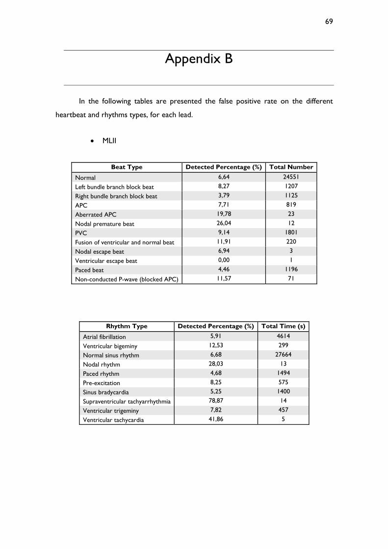
69
Appendix B
In the following tables are presented the false positive rate on the different
heartbeat and rhythms types, for each lead.
MLII
Beat Type Detected Percentage (%) Total Number
Normal 6,64 24551
Left bundle branch block beat 8,27 1207
Right bundle branch block beat 3,79 1125
APC 7,71 819
Aberrated APC 19,78 23
Nodal premature beat 26,04 12
PVC 9,14 1801
Fusion of ventricular and normal beat 11,91 220
Nodal escape beat 6,94 3
Ventricular escape beat 0,00 1
Paced beat 4,46 1196
Non-conducted P-wave (blocked APC) 11,57 71
Rhythm Type Detected Percentage (%) Total Time (s)
Atrial fibrillation 5,91 4614
Ventricular bigeminy 12,53 299
Normal sinus rhythm 6,68 27664
Nodal rhythm 28,03 13
Paced rhythm 4,68 1494
Pre-excitation 8,25 575
Sinus bradycardia 5,25 1400
Supraventricular tachyarrhythmia 78,87 14
Ventricular trigeminy 7,82 457
Ventricular tachycardia 41,86 5

70
V1
Beat Type Detected Percentage (%) Total Number
Normal 7,05 18917
Left bundle branch block beat 5,66 3430
Right bundle branch block beat 7,77 1887
APC 4,50 364
Aberrated APC 8,58 68
Nodal premature beat 0,00 1
PVC 10,16 1936
Fusion of ventricular and normal beat 24,81 249
Atrial escape beat 3,89 10
Nodal escape beat 8,47 99
Ventricular escape beat 0,63 105
Paced beat 7,69 2202
Fusion of paced and normal beat 8,37 150
Ventricular flutter wave 19,03 193
Non-conducted P-wave (blocked APC) 7,57 94
Rhythm Type Detected Percentage (%) Total Time (s)
Atrial bigeminy 1,92 117
Atrial fibrillation 3,43 2816
Atrial flutter 3,70 420
Ventricular bigeminy 11,01 1133
2º heart block 23,94 520
Idioventricular rhythm 1,09 157
Normal sinus rhythm 7,24 22619
Nodal rhythm 7,67 158
Paced rhythm 7,76 2921
Pre-excitation 6,28 604
Supraventricular tachyarrhythmia 1,26 85
Ventricular trigeminy 3,46 408
Ventricular flutter 18,06 93
Ventricular tachycardia 16,36 50

71
V2
Beat Type Detected Percentage (%) Total Number
Normal 4,25 2049
PVC 6,94 4
Paced beat 6,04 1951
Fusion of paced and normal beat 13,75 432
Unclassifiable beat 0,00 3
Rhythm Type Detected Percentage (%) Total Time (s)
Normal sinus rhythm 5,12 2983
Paced rhythm 6,50 2778
V5
Beat Type Detected Percentage (%) Total Number
Normal 3,77 3523
APC 3,47 24
Nodal premature beat 0,00 2
PVC 7,30 35
Fusion of ventricular and normal beat 0,00 2
Paced beat 5,79 1961
Fusion of paced and normal beat 19,22 427
Unclassifiable beat 0,00 3
Rhythm Type Detected Percentage (%) Total Time (s)
Normal sinus rhythm 4,64 4929
Paced rhythm 6,44 2780
Supraventricular tachyarrhythmia 0,00 7