1

Forecasting of Jet Fuel (ATF) consumption in India

2

Abstract

Airline companies, being the single largest user of jet fuel, are exposed to price

risk owing to extreme volatility in prices worldwide. Thus it is inevitable to

forecast the demand of aviation fuel turbine. In this project we did forecasting

of ATF consumption. The factors that affect the ATF consumption is crude oil

price, passengers carried for that particular time frame and ATF price. Many

methods can be used for forecasting ATF consumption but in most of the

literature review the method used was ARIMA method. We used ARIMA

method for forecasting the ATF consumption. More importantly the study

identifies the difference between the past actual ATF consumption and forecast.

We also try to correlate the ATF price and Crude oil price. This correlation

factor helps to find out the hedging ratio to hedge the ATF price with respect to

Crude oil price as jet fuel is no available on the trade exchange. This hedging

ratio helpful for speculation and forward and future contract of ATF.

3

Introduction

Aviation turbine fuel (ATF) or jet fuel is a specialized type of petroleum-based

fuel used to power aircrafts. It is generally of a higher quality than fuels used in

less critical applications such as heating or road transport. Aviation turbine fuel

(ATF) is extracted from the middle of fractional distillation process. Aviation

turbine fuel is a limited natural resource which is non-renewable and several

reports show that the world's crude oil production is close to the maximum level

and then it will start to decrease after reaching this maximum. It is estimated

that same effect on aviation fuel production as a crude oil production

declination. It is predicted by the aviation industry that aviation traffic will keep

on increasing.

Domestic production of jet fuel topped 22 billion gallons in 2012. However, the

consumption of jet fuel can vary, depending on imports and exports of the fuel.

Domestic fuel consumption by U.S. carriers was just over 17 billion gallons in

2012. Jet fuel purchasers include airlines, FBOs, airport owners and operators,

corporations with flight departments, operators of crop dusters and helicopters,

and the military. Traffic is predicted to grow by 5% per year to 2026, fuel

demand by about 3% per year in India. Indigenous production of ATF in India

in 2007 was 7,805,000 tones. India is self-sufficient in production of these

products with exports of 3,662,000 tones.

Airline companies, being the single largest user of jet fuel, are exposed to price

risk owing to extreme volatility in prices worldwide.The pricing of kerosene is

revised by these companies dynamically in tandem with international rates.

Typically, airlines have to either absorb the price volatility or pass the same to

consumers.

Thus it is inevitable to forecast the demand of aviation fuel turbine. The forecast

of demand will be carried out on the basis time series analysis which is based on

the past demand which help to find the future demand.

Factors affecting consumption

ATF prices

Efficiency

ATF consumption

Aviation industry demand – domestic and international (air traffic, etc.)

4

Environment friendly

In this project we are going to forecast the demand of ATF based on past data

analysis. The data we have taken is from ministry of petroleum and natural gas.

Rationale behind the project:

One of the reasons for the airlines industries struggling in India is the high price

of aviation turbine fuel (ATF) which has been eroding their bottom lines. The

prices of the ATF keep fluctuating which causes airlines to operate at a higher

cost and as a result their profit declines.

If reliable forecast of demand for ATF is known for the coming months or

years, then a proper planning can be done in terms of acquiring fuel using

different strategies such as hedging which helps in reducing the risk caused due

to variability of prices and thus helps in achieving sustainable growth.

Based on the issues mentioned below, we planned to carry out demand

forecasting of Aviation fuel in India:

Aviation Turbine Fuel (ATF) prices in India are higher than the international

market. The airline industry’s operational cost component is dominated by the

cost of the (ATF). The ATF price accounts for nearly 45% of the operational

expenses. A 10% increase in fuel price would push up costs by at least 4%, thus

causing a damper on the financial health of an airline business.

The operational cost of an airline significantly depends on the fuel prices.

Rising fuel prices affect the airline profitability and have a cascading effect on

the other supporting services of the aviation industry.

Literature Review:

Majorly all the reports of aviation industries are based on the traffic forecast,

carbon dioxide emission levelforecast, trends in fuel price and efficiency. To

understand aviation industry and jet fuel consumption, we review various

forecasting reports of the aviation industry as well as other petroleum industries.

5

Name of Report Forecasted Factor

Name

Publisher Source

Forecasting

Automobile Petrol

Demand in Australia

Automobile

Petrol

Institute of

Transport and

Logistics

Studies

bic.asn.au/_literat

ure_93796/Foreca

sting_Future_Fuel

_Demand

Aviation Turbine Fuel Crude-ATF

Correlation

MCX, India http://www.mcxin

dia.com/Uploads/

Products/240/Engl

ish_atf.pdf

An Overview of

Aviation -Fuel

Markets

for Biofuels

Stakeholders

Jet Fuel Price and

Jet Fuel

Consumption

National

Renewable

Energy

Laboratory

(NREL)

http://www.nrel.g

ov/docs/fy14osti/6

0254.pdf

Demand Forecast of

Petroleum Product

Consumption in the

Chinese

Transportation

Industry

Petroleum

Product

energies www.mdpi.com/jo

urnal/energies

Carbon Mitigation in

Indian Aviation by

Blending Jet Fuel with

Biofuels

Jet Fuel

Consumption

International

Journal of

Engineering

Research and

Development

www.ijerd.com

Table 1: Various Litterateurs and their sources

Automobile Petrol demand forecasting:

Source: (Li, 2008)

In this report Australia’s automobile petrol demand from 2007 through to 2020

is presented under the “business-as-usual” scenario. Different types of

modelling methods have been used to estimate petrol demand, each having

methodological strengths and weaknesses. This paper consist an ongoing need

to review the effectiveness of empirical fuel demand forecasting models, with a

focus on theoretical as well as practical considerations in the model-building

6

processes of different model forms. It consider a linear trend model, a quadratic

trend model, an exponential trend model, a single exponential smoothing model,

a Holt’s linear model, a Holt-Winters’ model, a partial adjustment model

(PAM) and an autoregressive integrated moving average (ARIMA) model. This

paper concludes that for the seasonal data, the best-forecasting model is the

quadratic trend model and for the non seasonal data, the same model produced

the most accurate short-term forecast.

For Jet Fuel price Forecast:

Source: (Aviation Turbine Fuel, 2008)

Aviation Turbine Fuel report is prepared by MCX, India. This report helpful to

understand the crude price and jet fuel price correlation. Jet fuel price is highly

dependent on the price of crude oil. Jet fuel prices are higher than crude oil

prices and generally correlate with crude oil price trends. Overall, jet fuel price

is determined by spot market prices, the terms of purchase contracts, and the

location of the purchase. Other determining factors include outside influences,

such as refinery shut downs; sudden, localized changes or seasonal shifts in

demand; interruptions in supply (e.g., natural disasters); and market speculation

and environmental regulations. Factors affecting prices are mainly crude oil

prices, aviation industry demand, political risk, forex fluctuation, Globalevnets.

Source: (Carolyn Davidson, 2014)

This report is intended for biofuels stakeholders who are interested in, but

unfamiliar with, theU.S. Aviation industry and, in particular, the aviation fuel

market. It provides an overview of the state of the aviation fuel industry,

targeting background information for evaluating the potential of biofuels in

aviation. This report includes jet fuel prices, consumption of jet fuel data and

forecasting of jet fuel price.

Fuel Efficient Forecast: The need for airlines to be more fuel efficient will be

driven in the coming years both by high fuel prices and environmental taxes or

caps. Past trends in fuel efficiency vary considerably depending on the measure

and the period chosen. However, there are few forecasters predicting future

changes in efficiency of greater than 1-2% a year.

7

Demand Forecast of Petroleum Product Consumption in the Chinese

Transportation Industry:

Source: (Jian Chai, 2012)

In this paper, petroleum product (mainly petrol and diesel) consumption in the

transportation sector of China is analysed. This was based on the Bayesian

linear regression theory and Markov Chain Monte Carlo method (MCMC),

establishing a demand-forecast model of petrol and diesel consumption. They

forecast the future consumer demand for oil products during “The 12th Five

Year Plan” (2011–2015) based on the historical data covering from 1985 to

2009. In the process of empirical analysis in this paper, we introduce five

explanatory variables into the model: urbanization level, per capita GDP,

turnover of passenger in aggregate (TPA), turnover of freight in aggregate

(TFA), and civilian vehicle number (CVN).

By using these forecasting methods they conclude that with some confidence

that the level of urbanization is a comprehensive factor. Comparing household

per capita annual expenditures in transport and communication, urban residents’

consumption level is far higher than that of rural residents.

Consumption of jet fuel:

Source: (Kowtham Kumar K, 2013)

“Carbon Mitigation in Indian Aviation by Blending Jet Fuel with Biofuels”

paper is prepared by Kowtham, B.Kaleeswaran, GeorgeMathew.K. in this paper

they forecasted the carbon mitigation level in the Indian aviation sector. The

International Air Transport Association has declared to cut its carbon emissions

to 50% by 2050. The National Biofuels Policy has also targeted to blend 20%

biofuels to its fossil fuel consumption. This paper aims in forecasting the jet fuel

demand for the Indian Aviation sector and the subsequent carbon mitigation

achieved by blending with biofuels. The utilization of the wastelands for the

biofuel production in various states of India has also been forecasted.To forecast

Consumption of jet fuel causal method can be used. This is the well-known

method available for forecasting and the most widely used. This method can be

used when historical data are available and the relationship between factors to

be forecasted and external factors are available.The linear regression method

was chosen over the causal regression because of the complexity. The linear

regression method involved a dependant variable related to an independent

variable by a linear equation.

8

Identify Gap:

This section will help us to differentiate our project with that available from the

different sources. The project that we found out over the web and what different

we are trying to do is briefed below:

One of the projects available was the forecasting of petroleum products based

on one of the forecasting method. We would be trying to use the same method

for the demand forecasting of ATF.

The other project we saw was showcasing the correlation between the price of

crude oil and ATF. On the same horizon we would like to obtain demand

forecast correlation between crude oil and ATF. This would help in planning

hedging strategies as crude oil traded in futures market while ATF is not traded.

We could use different methods to forecast the ATF demand. One available

paper used linear regression method to forecast the ATF demand, we would like

to use ARIMA technique of forecasting to do the same.

Relevance:

We came across many of the report based on forecasting of petroleum products

and correlation of crude oil price and ATF. We are trying to connect the

forecast of the petroleum products with forecast of ATF consumption based on

the trend analysis and on time series analysis. We hope the factors affecting

ATF consumption will be more or less the same as compared to petroleum

products. Also the methods used in petroleum product forecast will be helpful in

forecasting of ATF consumption.

The second paper we came across was forecast of crude oil prices, this paper is

relevant for knowing the trend analysis of the consumption of fuel and price

fluctuation based on it. This report on crude oil prices will provide the factor to

be considered in estimation of fluctuation of demand in crude which is similar

to estimate demand for ATF.

9

We will try to forecast ATF consumption based on the ARIMA and PAM

method which is used in automobile petroleum prices forecast , the paper which

we studied in literature review.

Contribution in the project

By studying various paper based on forecasting on petroleum products. The

forecast of ATF was not done and as the ATF industry is growing at fair rate

.The forecast for ATF will help for hedging.

We used ARIMA method to carry out forecast as in most of the paper studied

they used ARIMA, PAM, multiple regression method for analysis for trend

analysis. Our contribution to this forecast is different as compared to this paper

as we considered various variables that affected the ATF consumption.

Variables such as crude oil price, ATF price, passengers carried.

Research Design

Scientific problem

Forecasting of Jet fuel (ATF) consumption in India with the help of time series

data and finding the relation between crude oil price and jet fuel consumption

and price.

Research object

Forecast the Jet fuel consumption data for year 2015-2018 and find out

correlation between crude oil price and jet fuel consumption.

Research field

Forecasting techniques, correlation

Scientific hypothesis

If it develops a forecasting the jet fuel consumption based on past year data of

consumption and air traffic data, it helpful in speculating and hedging of jet fuel

consumption.

Independent variable

Jet fuel price, Crude oil price, air traffic data

10

Dependent variable

Jet fuel consumption

Research task

1. Facto-perceptible stage

Determination of historical development of jet fuel and its consumption

Literature survey for the forecasting methods and correlation method

Finding historic data of jet fuel consumption, air traffic and crude oil

price.

2. Data and analysis stage

Prepare data file in spps and other software

Create a forecasting model and analysis of data

Correlation between crude oil and jet fuel consumptio

3. Application stage

• Validation of the results obtained by developed forecasting model in spss

Understanding of outcomes and result .

Methodological Design

Research type and general goal

• The proposed research is applied, descriptive and time series analysis

• The proposed research is developed from quantitative point of view.

Population and sample

• The population of the proposed research is formed by ministry of oil and gas,

India.

• The population represents a sample of yearly jet fuel consumption, air traffic

and crude oil prices in India.

Methods and Techniques

In this research we will use the following methods to accomplish the

11

Proposed tasks:

• The Regression method will be used to relate the jet fuel consumption and air

traffic data.

• The ARIMA method will be used to forecast the jet fuel consumption.

Tools

• Statistical Package for the Social Sciences (SPSS) version 22

Data collection methods

The data collected is secondary data, also the data collected is

quantitative type of data.

Data collected is month wise data for consumption of ATF, ATF price,

crude oil price, passengers carried.

Data collected is from

o www.indexmundi.com

o www.indiastate.com

o www.dgh.com

Data analysis and interpretation

Hedging:

Hedging is a tool to reduce risk in the business by taking opposite position in

the spot and the futures market. Airlines companies face risk of fluctuating jet

fuel prices. ATF fuel is not traded in futures market and in order to reduce this

risk arising from price volatility, Airlines Company goes for hedging of crude

oil as ATF and crude oil prices are correlated. Recently it was in news that AIR

INDIA is conducting large scale hedging of jet fuel for the first time to take the

advantage of falling crude oil prices.

Correlation factor:

CORRELATIONS

/VARIABLES=ATF_PriceCrude_oil_Price

12

/PRINT=TWOTAIL NOSIG

/MISSING=PAIRWISE.

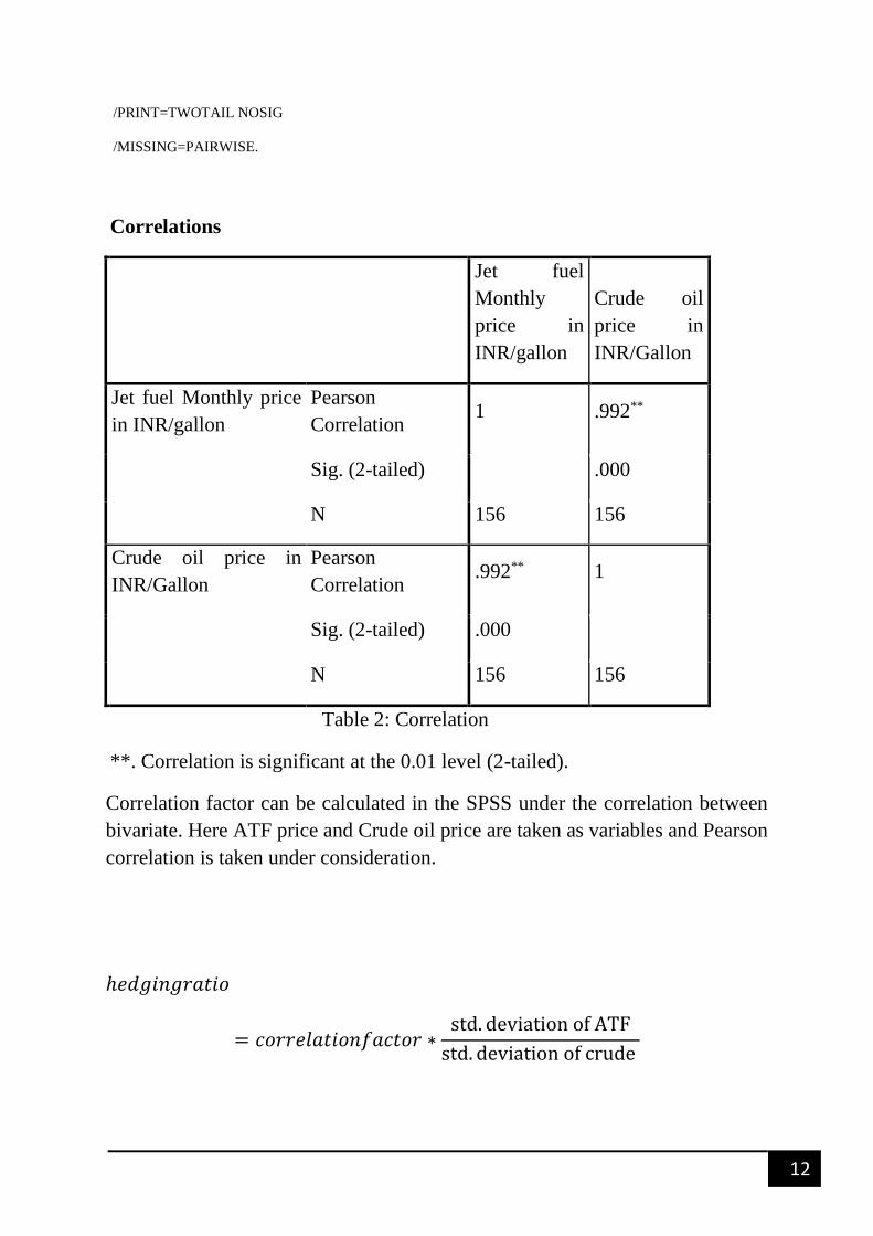
Correlations

Jet fuel

Monthly

price in

INR/gallon

Crude oil

price in

INR/Gallon

Jet fuel Monthly price

in INR/gallon

Pearson

Correlation 1 .992**

Sig. (2-tailed) .000

N 156 156

Crude oil price in

INR/Gallon

Pearson

Correlation .992** 1

Sig. (2-tailed) .000

N 156 156

Table 2: Correlation

**. Correlation is significant at the 0.01 level (2-tailed).

Correlation factor can be calculated in the SPSS under the correlation between

bivariate. Here ATF price and Crude oil price are taken as variables and Pearson

correlation is taken under consideration.

ℎ𝑒𝑑𝑔𝑖𝑛𝑔𝑟𝑎𝑡𝑖𝑜

= 𝑐𝑜𝑟𝑟𝑒𝑙𝑎𝑡𝑖𝑜𝑛𝑓𝑎𝑐𝑡𝑜𝑟 ∗std. deviation of ATF

std. deviation of crude

13

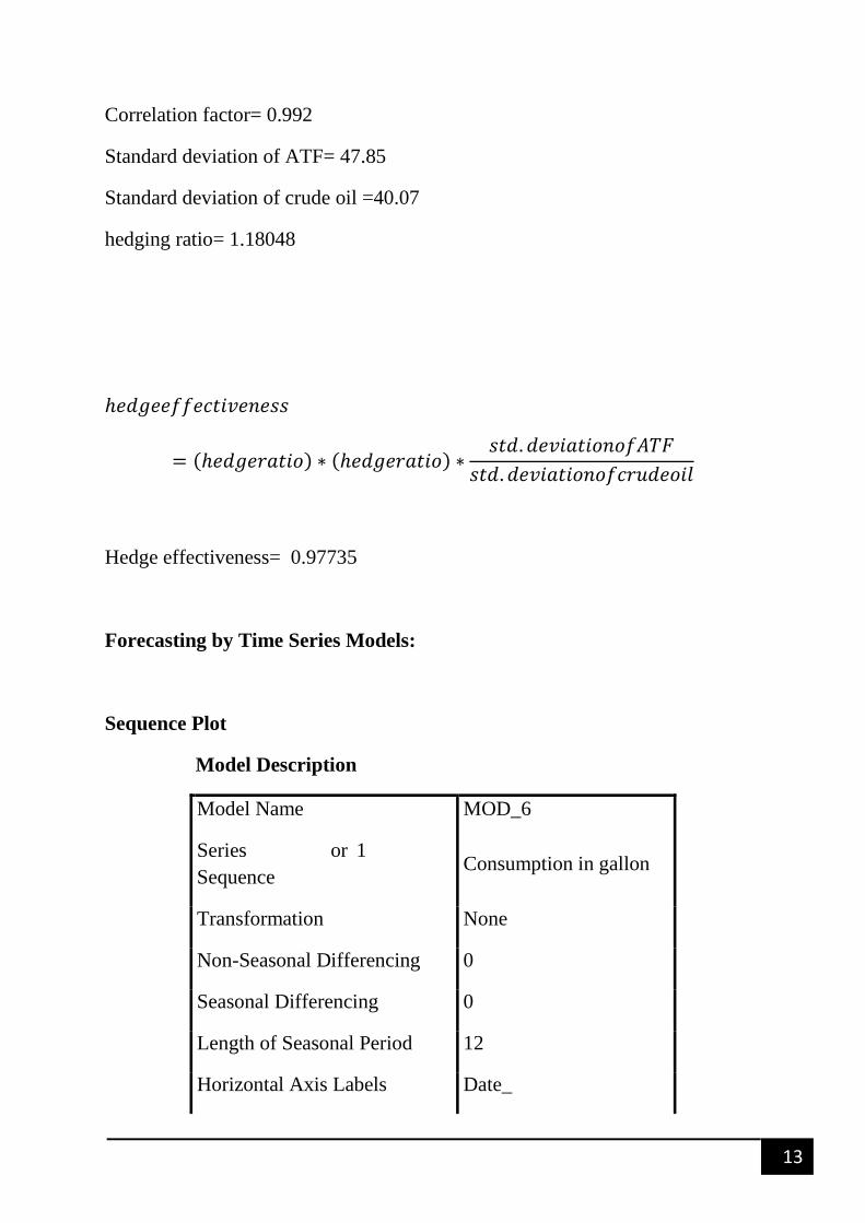
Correlation factor= 0.992

Standard deviation of ATF= 47.85

Standard deviation of crude oil =40.07

hedging ratio= 1.18048

ℎ𝑒𝑑𝑔𝑒𝑒𝑓𝑓𝑒𝑐𝑡𝑖𝑣𝑒𝑛𝑒𝑠𝑠

= (ℎ𝑒𝑑𝑔𝑒𝑟𝑎𝑡𝑖𝑜) ∗ (ℎ𝑒𝑑𝑔𝑒𝑟𝑎𝑡𝑖𝑜) ∗𝑠𝑡𝑑. 𝑑𝑒𝑣𝑖𝑎𝑡𝑖𝑜𝑛𝑜𝑓𝐴𝑇𝐹

𝑠𝑡𝑑. 𝑑𝑒𝑣𝑖𝑎𝑡𝑖𝑜𝑛𝑜𝑓𝑐𝑟𝑢𝑑𝑒𝑜𝑖𝑙

Hedge effectiveness= 0.97735

Forecasting by Time Series Models:

Sequence Plot

Model Description

Model Name MOD_6

Series or

Sequence

1 Consumption in gallon

Transformation None

Non-Seasonal Differencing 0

Seasonal Differencing 0

Length of Seasonal Period 12

Horizontal Axis Labels Date_

14

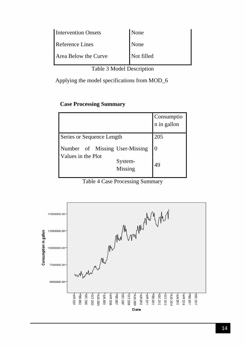
Intervention Onsets None

Reference Lines None

Area Below the Curve Not filled

Table 3 Model Description

Applying the model specifications from MOD_6

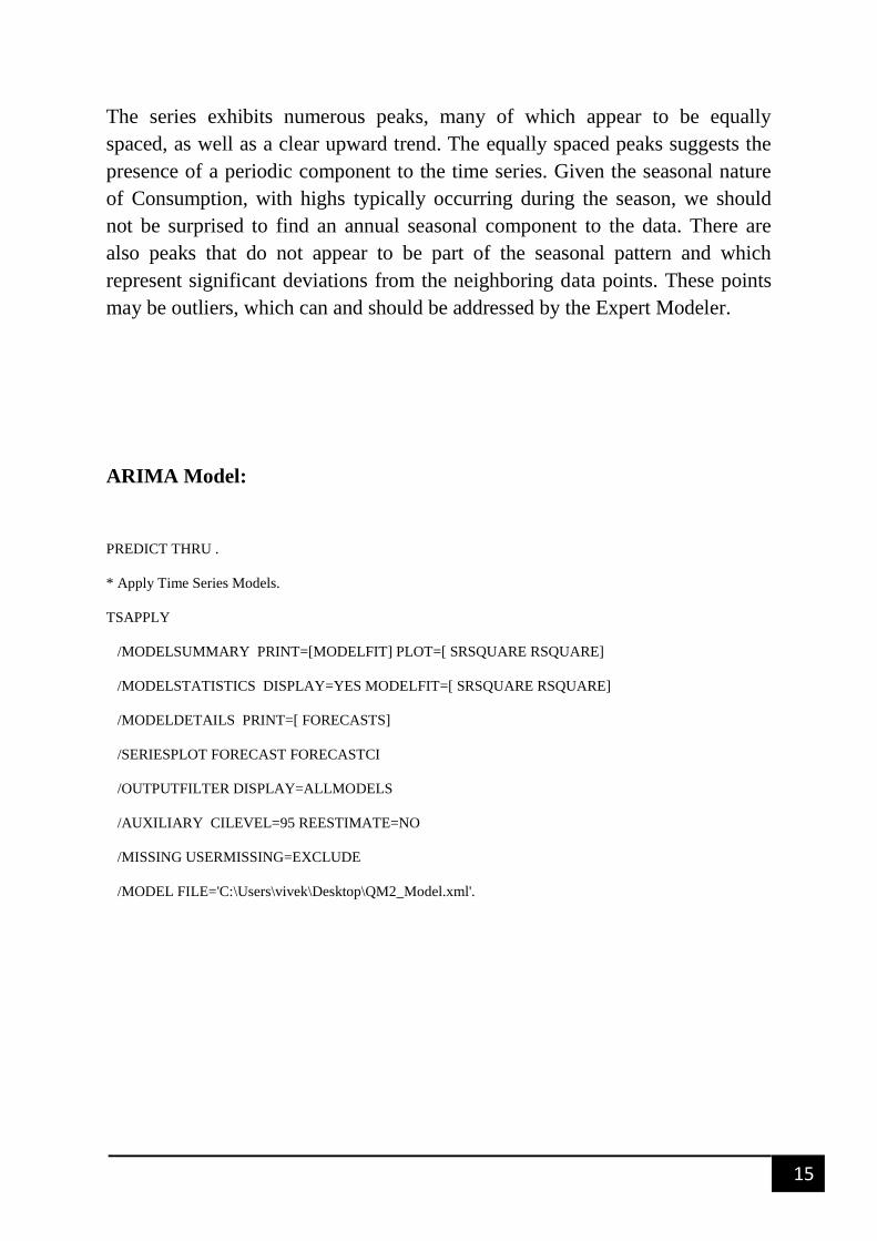
Case Processing Summary

Consumptio

n in gallon

Series or Sequence Length 205

Number of Missing

Values in the Plot

User-Missing 0

System-

Missing 49

Table 4 Case Processing Summary

15

The series exhibits numerous peaks, many of which appear to be equally

spaced, as well as a clear upward trend. The equally spaced peaks suggests the

presence of a periodic component to the time series. Given the seasonal nature

of Consumption, with highs typically occurring during the season, we should

not be surprised to find an annual seasonal component to the data. There are

also peaks that do not appear to be part of the seasonal pattern and which

represent significant deviations from the neighboring data points. These points

may be outliers, which can and should be addressed by the Expert Modeler.

ARIMA Model:

PREDICT THRU .

* Apply Time Series Models.

TSAPPLY

/MODELSUMMARY PRINT=[MODELFIT] PLOT=[ SRSQUARE RSQUARE]

/MODELSTATISTICS DISPLAY=YES MODELFIT=[ SRSQUARE RSQUARE]

/MODELDETAILS PRINT=[ FORECASTS]

/SERIESPLOT FORECAST FORECASTCI

/OUTPUTFILTER DISPLAY=ALLMODELS

/AUXILIARY CILEVEL=95 REESTIMATE=NO

/MISSING USERMISSING=EXCLUDE

/MODEL FILE='C:\Users\vivek\Desktop\QM2_Model.xml'.

16

Apply Time Series Models

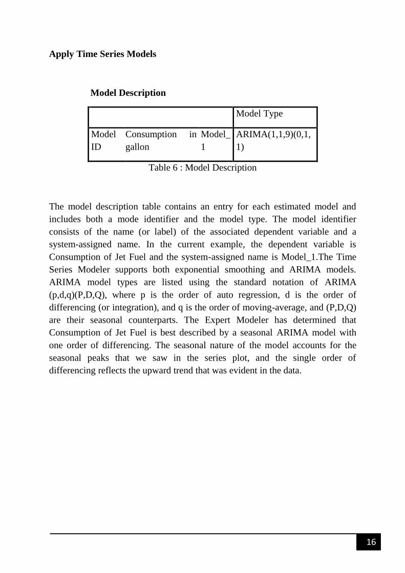
Model Description

Model Type

Model

ID

Consumption in

gallon

Model_

1

ARIMA(1,1,9)(0,1,

1)

Table 6 : Model Description

The model description table contains an entry for each estimated model and

includes both a mode identifier and the model type. The model identifier

consists of the name (or label) of the associated dependent variable and a

system-assigned name. In the current example, the dependent variable is

Consumption of Jet Fuel and the system-assigned name is Model_1.The Time

Series Modeler supports both exponential smoothing and ARIMA models.

ARIMA model types are listed using the standard notation of ARIMA

(p,d,q)(P,D,Q), where p is the order of auto regression, d is the order of

differencing (or integration), and q is the order of moving-average, and (P,D,Q)

are their seasonal counterparts. The Expert Modeler has determined that

Consumption of Jet Fuel is best described by a seasonal ARIMA model with

one order of differencing. The seasonal nature of the model accounts for the

seasonal peaks that we saw in the series plot, and the single order of

differencing reflects the upward trend that was evident in the data.

17

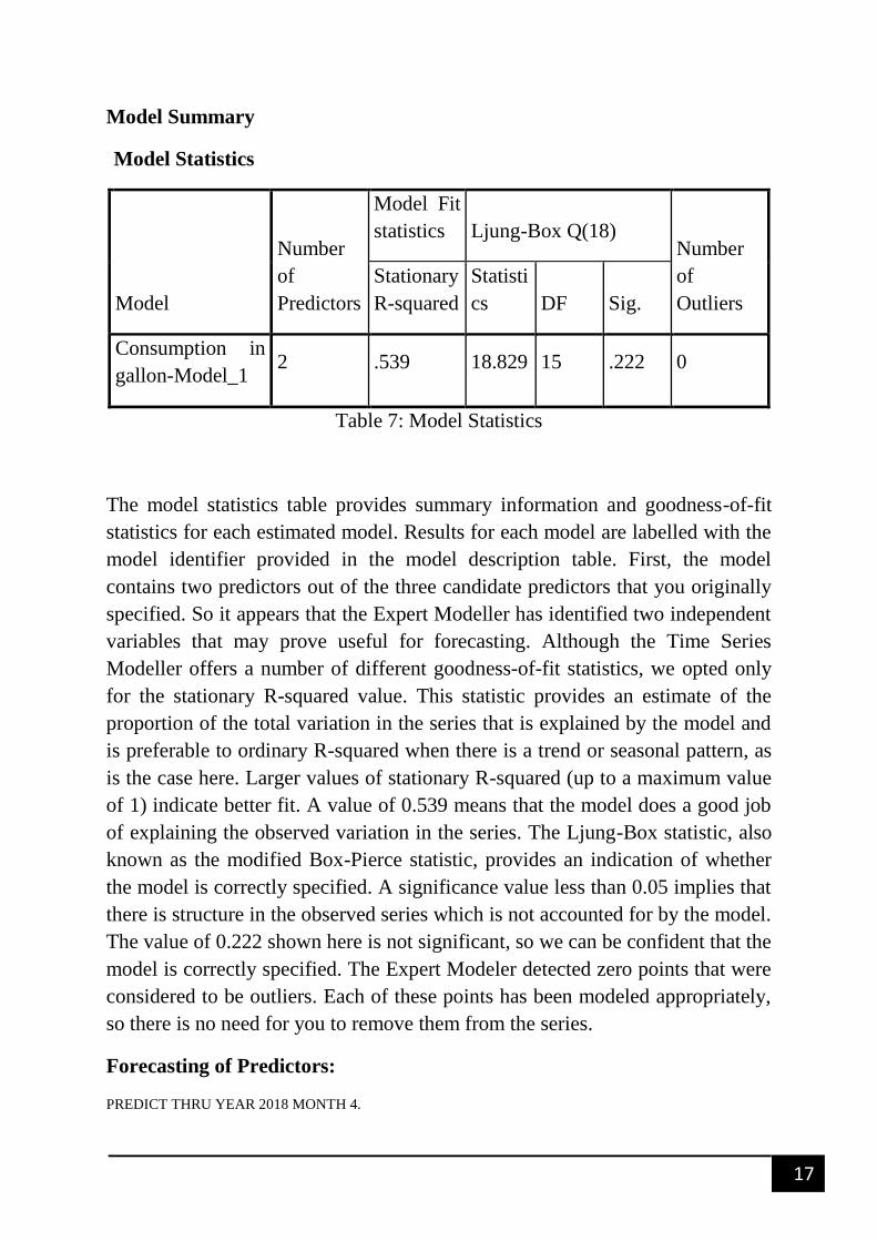
Model Summary

Model Statistics

Model

Number

of

Predictors

Model Fit

statistics Ljung-Box Q(18) Number

of

Outliers

Stationary

R-squared

Statisti

cs DF Sig.

Consumption in

gallon-Model_1 2 .539 18.829 15 .222 0

Table 7: Model Statistics

The model statistics table provides summary information and goodness-of-fit

statistics for each estimated model. Results for each model are labelled with the

model identifier provided in the model description table. First, the model

contains two predictors out of the three candidate predictors that you originally

specified. So it appears that the Expert Modeller has identified two independent

variables that may prove useful for forecasting. Although the Time Series

Modeller offers a number of different goodness-of-fit statistics, we opted only

for the stationary R-squared value. This statistic provides an estimate of the

proportion of the total variation in the series that is explained by the model and

is preferable to ordinary R-squared when there is a trend or seasonal pattern, as

is the case here. Larger values of stationary R-squared (up to a maximum value

of 1) indicate better fit. A value of 0.539 means that the model does a good job

of explaining the observed variation in the series. The Ljung-Box statistic, also

known as the modified Box-Pierce statistic, provides an indication of whether

the model is correctly specified. A significance value less than 0.05 implies that

there is structure in the observed series which is not accounted for by the model.

The value of 0.222 shown here is not significant, so we can be confident that the

model is correctly specified. The Expert Modeler detected zero points that were

considered to be outliers. Each of these points has been modeled appropriately,

so there is no need for you to remove them from the series.

Forecasting of Predictors:

PREDICT THRU YEAR 2018 MONTH 4.

18

* Time Series Modeler.

TSMODEL

/MODELSUMMARY PRINT=[MODELFIT]

/MODELSTATISTICS DISPLAY=YES MODELFIT=[ SRSQUARE]

/MODELDETAILS PRINT=[ FORECASTS]

/SERIESPLOT OBSERVED FORECAST

/OUTPUTFILTER DISPLAY=ALLMODELS

/SAVE PREDICTED(Predicted)

/AUXILIARY CILEVEL=95 MAXACFLAGS=24

/MISSING USERMISSING=EXCLUDE

/MODEL DEPENDENT=Crude_oil_PricePassengers_carriedATF_Price

PREFIX='Model'

/EXPERTMODELER TYPE=[ARIMA EXSMOOTH] TRYSEASONAL=YES

/AUTOOUTLIER DETECT=OFF.

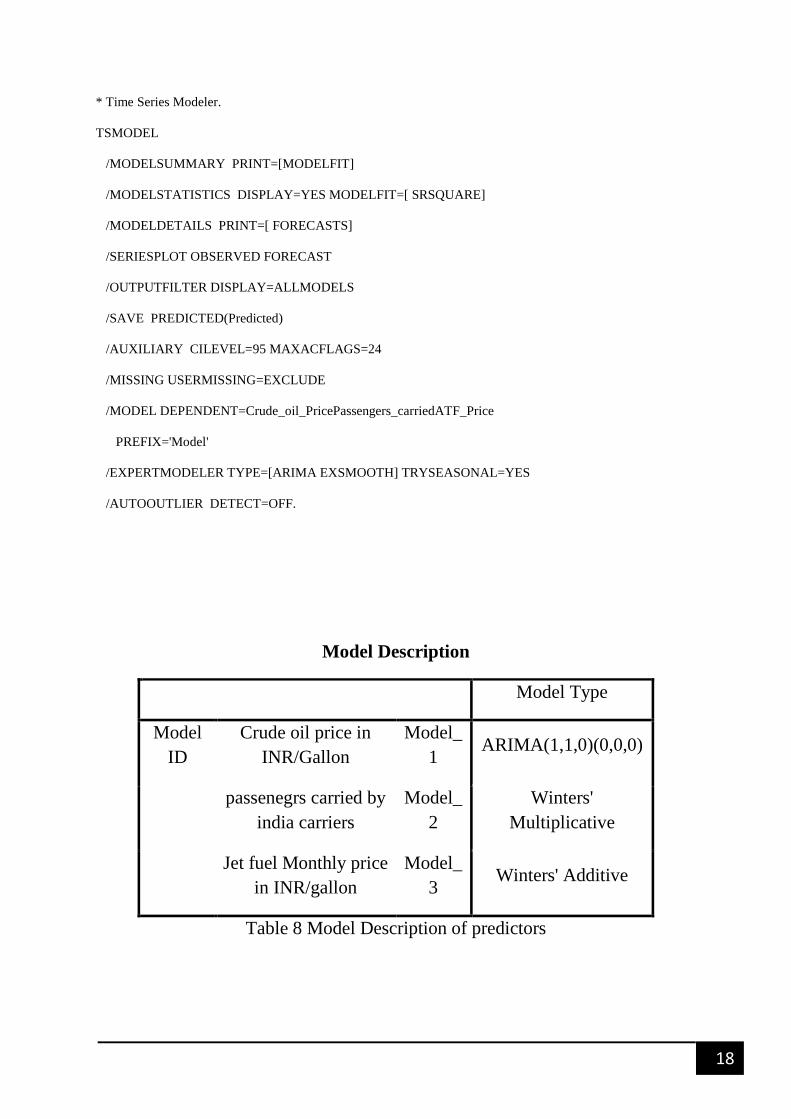
Model Description

Model Type

Model

ID

Crude oil price in

INR/Gallon

Model_

1 ARIMA(1,1,0)(0,0,0)

passenegrs carried by

india carriers

Model_

2

Winters'

Multiplicative

Jet fuel Monthly price

in INR/gallon

Model_

3 Winters' Additive

Table 8 Model Description of predictors

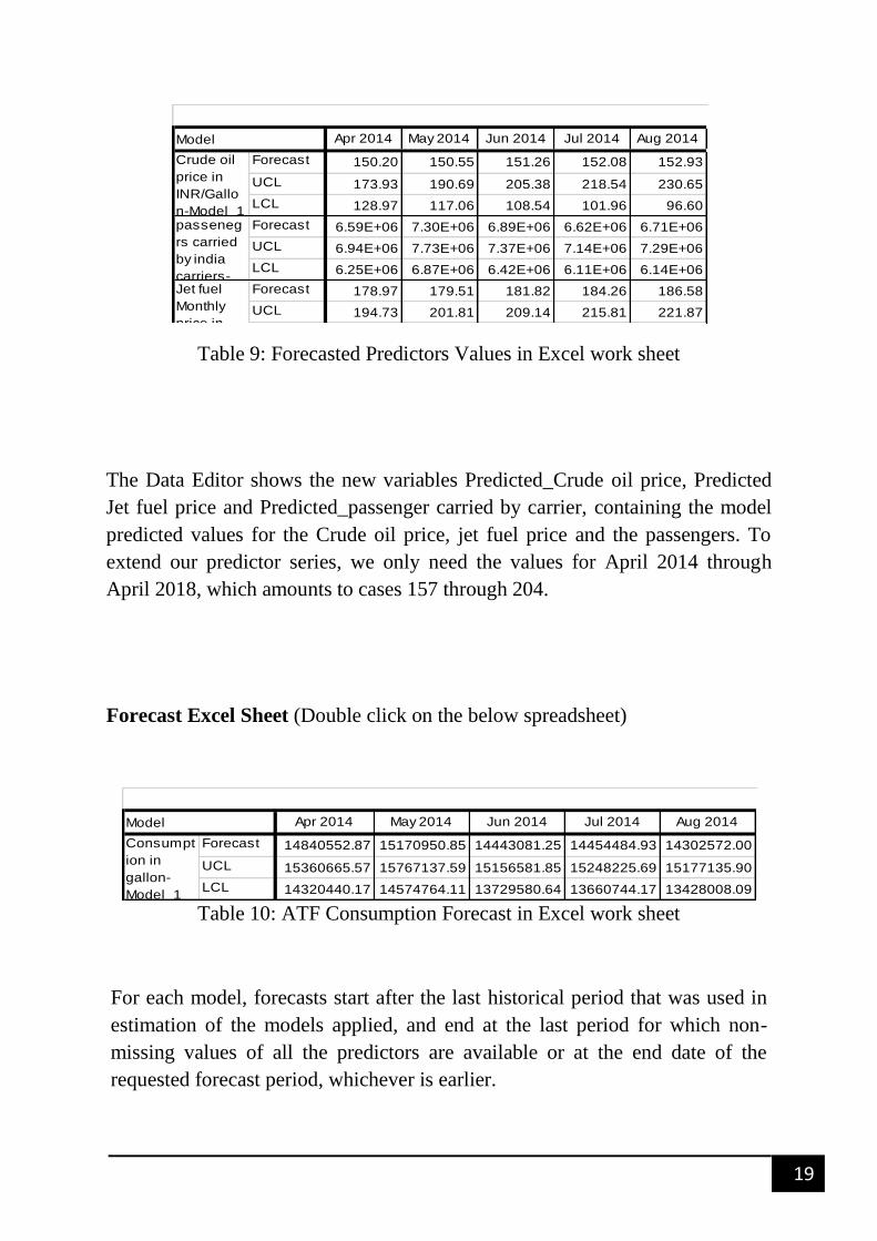
19

Table 9: Forecasted Predictors Values in Excel work sheet

The Data Editor shows the new variables Predicted_Crude oil price, Predicted

Jet fuel price and Predicted_passenger carried by carrier, containing the model

predicted values for the Crude oil price, jet fuel price and the passengers. To

extend our predictor series, we only need the values for April 2014 through

April 2018, which amounts to cases 157 through 204.

Forecast Excel Sheet (Double click on the below spreadsheet)

Apr 2014 May 2014 Jun 2014 Jul 2014 Aug 2014

Forecast 14840552.87 15170950.85 14443081.25 14454484.93 14302572.00

UCL 15360665.57 15767137.59 15156581.85 15248225.69 15177135.90

LCL 14320440.17 14574764.11 13729580.64 13660744.17 13428008.09

Forecast

Model

Consumpt

ion in

gallon-

Model_1

Table 10: ATF Consumption Forecast in Excel work sheet

For each model, forecasts start after the last historical period that was used in

estimation of the models applied, and end at the last period for which non-

missing values of all the predictors are available or at the end date of the

requested forecast period, whichever is earlier.

Apr 2014 May 2014 Jun 2014 Jul 2014 Aug 2014

Forecast 150.20 150.55 151.26 152.08 152.93

UCL 173.93 190.69 205.38 218.54 230.65

LCL 128.97 117.06 108.54 101.96 96.60

Forecast 6.59E+06 7.30E+06 6.89E+06 6.62E+06 6.71E+06

UCL 6.94E+06 7.73E+06 7.37E+06 7.14E+06 7.29E+06

LCL 6.25E+06 6.87E+06 6.42E+06 6.11E+06 6.14E+06

Forecast 178.97 179.51 181.82 184.26 186.58

UCL 194.73 201.81 209.14 215.81 221.87

Forecast

Model

Crude oil

price in

INR/Gallo

n-Model_1passeneg

rs carried

by india

carriers-Jet fuel

Monthly

price in

INR/gallon-

20

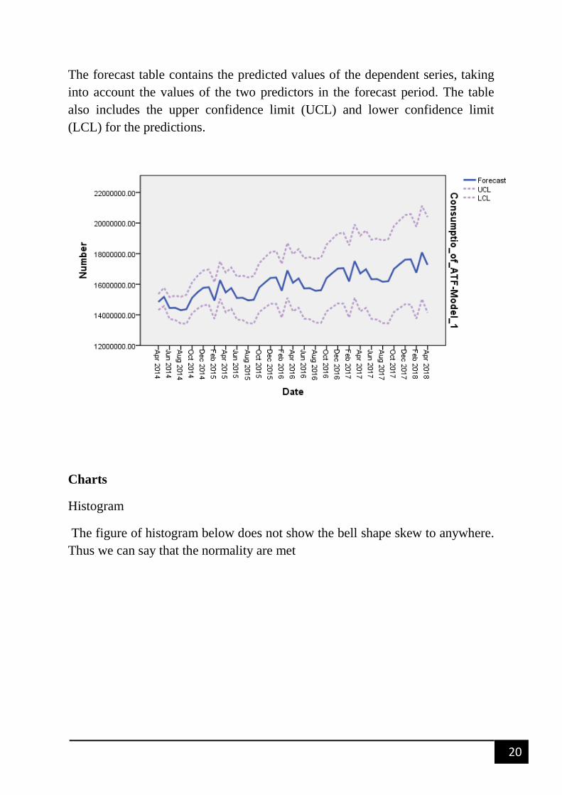
The forecast table contains the predicted values of the dependent series, taking

into account the values of the two predictors in the forecast period. The table

also includes the upper confidence limit (UCL) and lower confidence limit

(LCL) for the predictions.

Charts

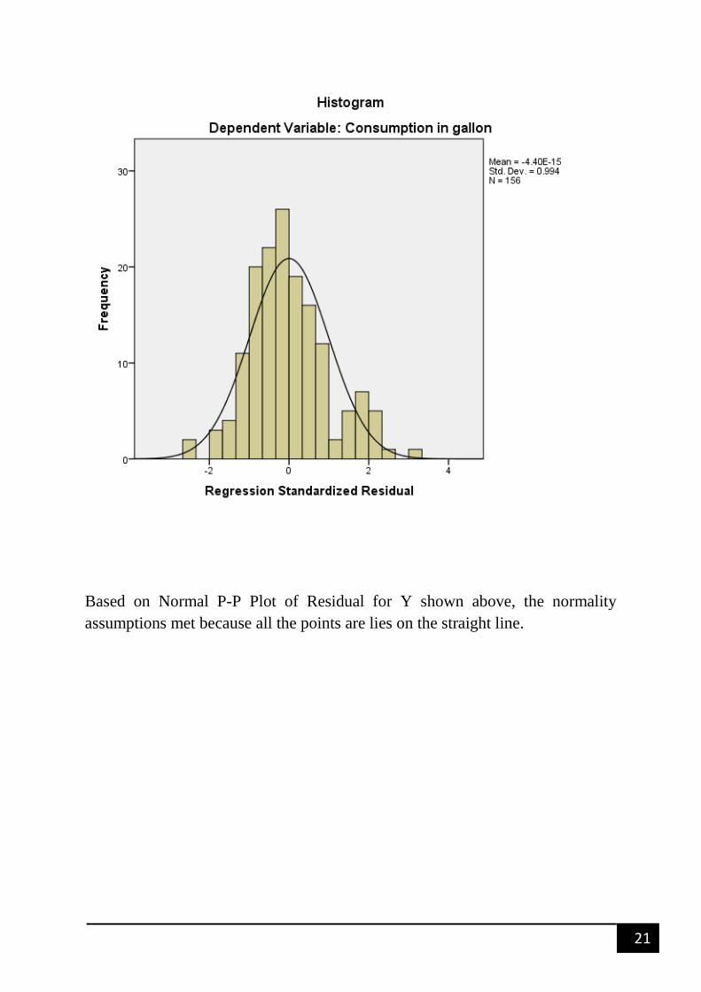
Histogram

The figure of histogram below does not show the bell shape skew to anywhere.

Thus we can say that the normality are met

21

Based on Normal P-P Plot of Residual for Y shown above, the normality

assumptions met because all the points are lies on the straight line.

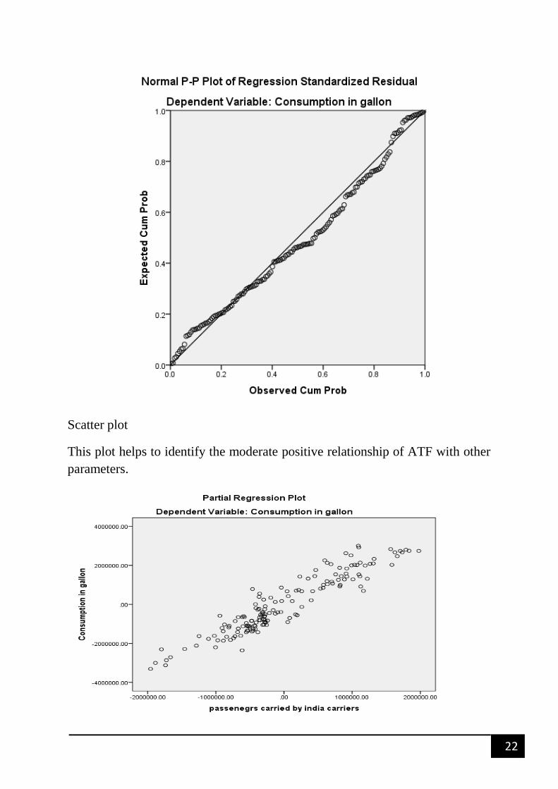
22

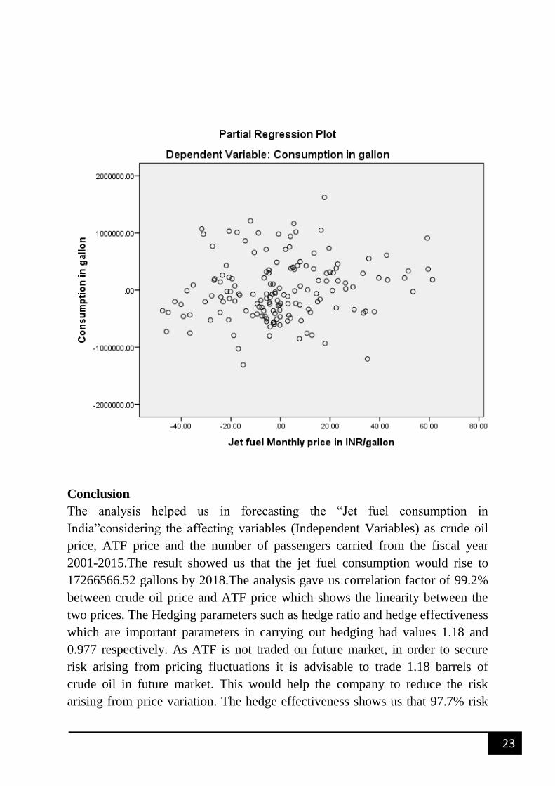
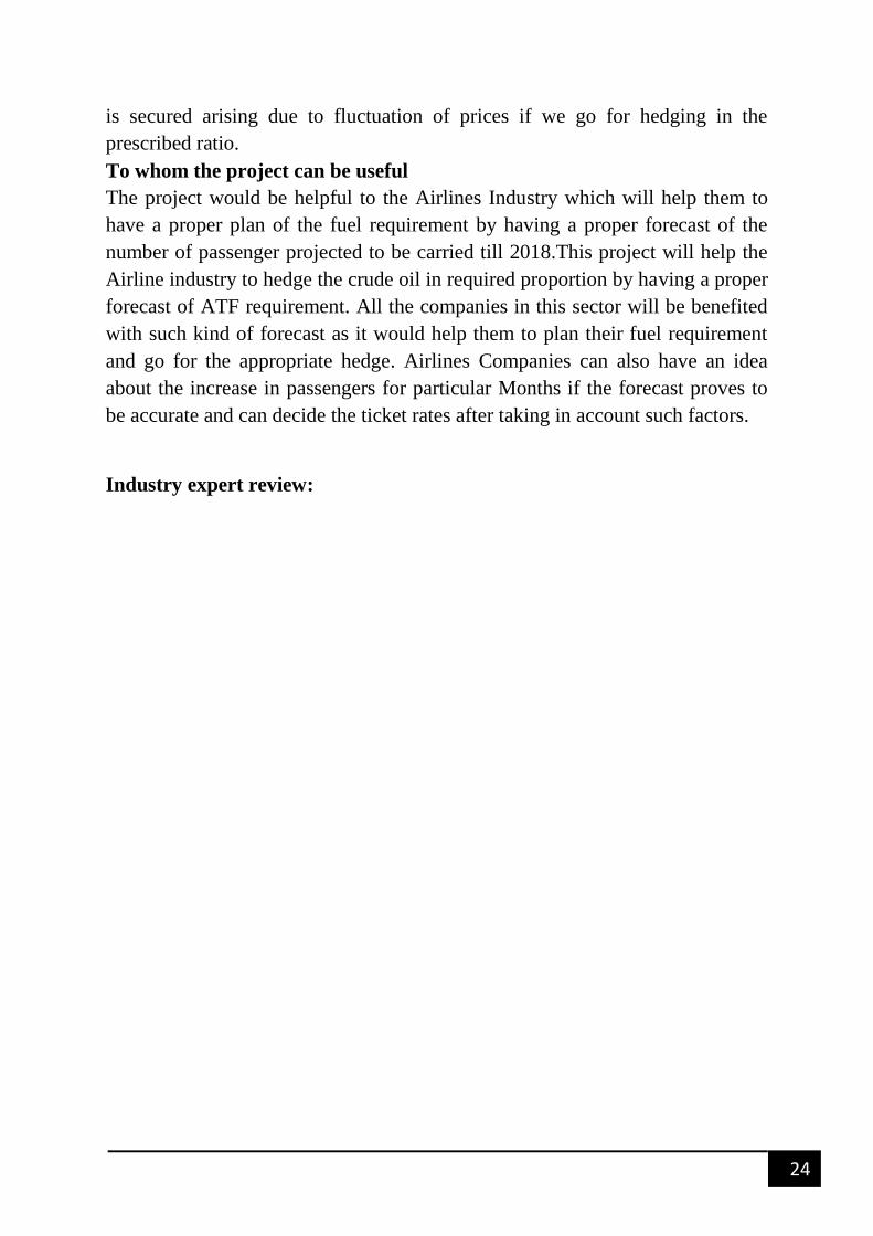
Scatter plot

This plot helps to identify the moderate positive relationship of ATF with other

parameters.

23

Conclusion

The analysis helped us in forecasting the “Jet fuel consumption in

India”considering the affecting variables (Independent Variables) as crude oil

price, ATF price and the number of passengers carried from the fiscal year

2001-2015.The result showed us that the jet fuel consumption would rise to

17266566.52 gallons by 2018.The analysis gave us correlation factor of 99.2%

between crude oil price and ATF price which shows the linearity between the

two prices. The Hedging parameters such as hedge ratio and hedge effectiveness

which are important parameters in carrying out hedging had values 1.18 and

0.977 respectively. As ATF is not traded on future market, in order to secure

risk arising from pricing fluctuations it is advisable to trade 1.18 barrels of

crude oil in future market. This would help the company to reduce the risk

arising from price variation. The hedge effectiveness shows us that 97.7% risk

24

is secured arising due to fluctuation of prices if we go for hedging in the

prescribed ratio.

To whom the project can be useful

The project would be helpful to the Airlines Industry which will help them to

have a proper plan of the fuel requirement by having a proper forecast of the

number of passenger projected to be carried till 2018.This project will help the

Airline industry to hedge the crude oil in required proportion by having a proper

forecast of ATF requirement. All the companies in this sector will be benefited

with such kind of forecast as it would help them to plan their fuel requirement

and go for the appropriate hedge. Airlines Companies can also have an idea

about the increase in passengers for particular Months if the forecast proves to

be accurate and can decide the ticket rates after taking in account such factors.

Industry expert review:

25

Bibliography

(2008). Aviation Turbine Fuel. Mumbai: MCX.

Carolyn Davidson, E. N. (2014). An Overview of Aviation Fuel Marketsfor

Biofuels Stakeholders. West parkway: National Renewable Energy Laboratry.

(2014). Global Market Forecast. Airbus.

Jian Chai, S. W. (2012). Demand Forecast of Petroleum Product Consumption

in the . Xi,an: energise.

Kowtham Kumar K, B. M. (2013). Carbon Mitigation in Indian Aviation by

Blending Jet . International Journal of Engineering Research and Development

, 43-46.

Li, Z. (2008). Forecasting Automobile Petrol Demand in Australia . Sydney.

MCX. (2008). Aviation Turbine Fuel. Mumbai: MCX.