Embed Size (px)
Citation preview
QC Reference Manual version 1.4
R. E. Miller and E. B. Tadmorwww.qcmethod.org
October 2011

Contents
1 Introduction 1
2 QC Code structure 32.1 Module mod global . . . . . . . . . . . . . . . . . . . . . . . . . . . . . . . . 52.2 QC Variables . . . . . . . . . . . . . . . . . . . . . . . . . . . . . . . . . . . 62.3 Module mod boundary . . . . . . . . . . . . . . . . . . . . . . . . . . . . . . 102.4 Module mod grain . . . . . . . . . . . . . . . . . . . . . . . . . . . . . . . . 102.5 Module mod mesh . . . . . . . . . . . . . . . . . . . . . . . . . . . . . . . . 122.6 Module mod output . . . . . . . . . . . . . . . . . . . . . . . . . . . . . . . 122.7 Module mod pload . . . . . . . . . . . . . . . . . . . . . . . . . . . . . . . . 152.8 Module mod qclib . . . . . . . . . . . . . . . . . . . . . . . . . . . . . . . . . 152.9 Module mod repatom . . . . . . . . . . . . . . . . . . . . . . . . . . . . . . . 162.10 Module mod stiff . . . . . . . . . . . . . . . . . . . . . . . . . . . . . . . . . 172.11 User-Specified Routines . . . . . . . . . . . . . . . . . . . . . . . . . . . . . . 17
2.11.1 user mesh . . . . . . . . . . . . . . . . . . . . . . . . . . . . . . . . . 182.11.2 user bcon . . . . . . . . . . . . . . . . . . . . . . . . . . . . . . . . . 322.11.3 user pdel . . . . . . . . . . . . . . . . . . . . . . . . . . . . . . . . . . 382.11.4 user potential . . . . . . . . . . . . . . . . . . . . . . . . . . . . . . . 402.11.5 user plot . . . . . . . . . . . . . . . . . . . . . . . . . . . . . . . . . . 44
3 Head Stage Commands 453.1 Macro ’cons’ : read in potential specific constitutive input . . . . . . . . . 453.2 Macro ’end ’ : terminate head stage . . . . . . . . . . . . . . . . . . . . . 473.3 Macro ’fact’ : sets global run factors . . . . . . . . . . . . . . . . . . . . . 473.4 Macro ’flag’ : sets global run flags . . . . . . . . . . . . . . . . . . . . . . 483.5 Macro ’grai’ : read in grain structure information, initialize grains . . . . 503.6 Macro ’mate’ : material data input . . . . . . . . . . . . . . . . . . . . . . 503.7 Macro ’mesh’ : generate mesh (user mesh routine) . . . . . . . . . . . . . . 513.8 Macro ’zone’ : define special-attribute zones . . . . . . . . . . . . . . . . . 51
4 Macros Stage Commands 524.1 Macro ’adap’ : Automatically adapt the mesh, through mesh refining and
coarsening . . . . . . . . . . . . . . . . . . . . . . . . . . . . . . . . . . . . . 524.2 Macro ’bcon’ : apply boundary conditions (user bcon routine) . . . . . . . 534.3 Macro ’chec’ : Numerical derivative check . . . . . . . . . . . . . . . . . . 534.4 Macro ’clea’ : Re-initialize solution variables. . . . . . . . . . . . . . . . . 554.5 Macro ’conv’ : Loop convergence test . . . . . . . . . . . . . . . . . . . . . 554.6 Macro ’dtim’ : set time increment . . . . . . . . . . . . . . . . . . . . . . . 564.7 Macro ’form’ : Form the out-of-balance force vector . . . . . . . . . . . . . 564.8 Macro ’ghos’ : Compute ghost forces correction . . . . . . . . . . . . . . . 574.9 Macro ’loop’ : set loop start indicators . . . . . . . . . . . . . . . . . . . . 584.10 Macro ’mark’ : set or return to a marked state of the simulation . . . . . . 584.11 Macro ’next’ : loop terminator control . . . . . . . . . . . . . . . . . . . . 59

4.12 Macro ’outp’ : output nodal displacements to the log file . . . . . . . . . . 604.13 Macro ’pdel’ : compute current external load and applied displacement . . 604.14 Macro ’plot’ : write out plot file in Tecplot R© format . . . . . . . . . . . . 614.15 Macro ’prop’ : define proportional load table . . . . . . . . . . . . . . . . . 654.16 Macro ’prot’ : protect existing nodes from being deleted by coarsening . . 664.17 Macro ’repo’ : print out current energy and out-of-balance forces . . . . . 674.18 Macro ’rest’ : read/write restart files . . . . . . . . . . . . . . . . . . . . . 674.19 Macro ’setp’ : store current resultant for comparison in conv,pdel . . . . 694.20 Macro ’solv’ : call solver routine . . . . . . . . . . . . . . . . . . . . . . . 694.21 Macro ’stat’ : Recompute local/nonlocal representative atom status . . . 704.22 Macro ’stpr’ : print state variables (stress, strain other elemental quantities) 724.23 Macro ’syst’ : compute system matrix and right-hand side concurrently . 724.24 Macro ’tang’ : form tangent stiffness . . . . . . . . . . . . . . . . . . . . . 734.25 Macro ’time’ : increment time . . . . . . . . . . . . . . . . . . . . . . . . . 734.26 Macro ’tole’ : set solution tolerance . . . . . . . . . . . . . . . . . . . . . 73

1.0 Introduction 1
1 Introduction
The quasicontinuum (QC) method is a multiscale method combining atomistic simulations
with nonlinear continuum finite elements. Theoretical details about the method are given in
a series of papers [1, 2, 3, 4, 5]. This manual describes the details of using the freely-available
QC method code distributed on the QC website www.qcmethod.org. The code is written in
Fortran 90 and is designed to be as portable as possible. It has been successfully tested with
a variety of different Fortran compilers1. Porting to new compilers and architectures should
be straightforward.
The current distribution version of the QC code has certain limitations:
• It is limited to two-dimensional boundary value problems that can be described with
displacement fields of the form
ux(x, y), uy(x, y), uz(x, y).
Despite the two-dimensional constraint, all atomistic calculations are performed in
three dimensions. This corresponds to simulating a slab with periodic boundary con-
ditions applied in the out-of-plane direction that has a thickness equal to the minimum
crystallographic repeat distance in that direction. This can be used, for example, to
correctly simulate a dislocation whose line is perpendicular to the simulation plane,
but not one inclined to it.
• The code is limited to crystalline materials with a simple lattice structure, such as fcc
and bcc metals. It is currently not possible to simulate complex crystal materials such
as hcp metals or unit cells containing multiple species. (It is possible to simulate a
system containing multiple simple crystals in separate grains.)
• The code is a static energy minimization code. It can be used to study equilibrium
structures at zero temperature, but not dynamical processes or finite temperature
1See Section 1.2 of the QC Tutorial Guide for a list of supported compilers.

1.0 Introduction 2
effects.
• The atomic interactions are limited to empirical potentials in which the energy of the
total system can be decomposed as a sum over individual atom energies. The current
implementation includes the embedded-atom method (EAM) potential [6]. It should
be straightforward to implement other potential forms.
These issues do not constitute limitations to the QC methodology itself (see for example [7]
for extension to three dimensions, [8, 9] for extension to complex crystals, [10] for extension
to finite temperature, and [11] for incorporation of quantum mechanical calculations within
QC). These developments are planned for future releases of the distribution code.
Performing a QC simulation requires the preparation of five user routines that are linked in
with the QC code2 and an input file containing a set of intstructions to the QC program
based on the simple command line interface originally provided with the program FEAP
[12]. This manual provides the information necessary to complete these two tasks. Section 2
provides an overview of the QC program structure along with information on how to prepare
the user routines. Sections 3 and 4 provide a listing of all the QC commands that can appear
in the input file, with details of the command syntax, options and function. QC simulations
are comprised of two stages, each with its own set of commands. Therefore, the listing is
split into the head stage commands (Section 3) and the macros stage commands (Section 4).
Within each stage, the commands are listed alphabetically.
For users that are unfamiliar with QC simulations, a good starting point is the QC
Tutorial Guide, which traces through a simple example simulation. This reference manual is
intended to provide complete detail of the user routines and input commands, but assumes
that the user is already familiar with the QC approach.
2For many simulations only one of the five user routines is required and the rest can be left blank.

2.0 QC Code Structure 3
2 QC Code structure
The QC code consists of one main file qcmain.f and a large number of additional files
beginning with the suffix mod each containing one Fortran 90 module dedicated to a specific
task or closely-related set of tasks. Each module contains routines and/or variables related
to its task. The QC modules and the tasks they deal with are:
• mod adaption.f: Automatic mesh refinement and coarsening.
• mod bandwidth.f: Nodal renumbering to minimize the stiffness matrix bandwidth.
• mod boundary.f: Model boundary and special-attribute zones. See a more detaileddescription in Section 2.3.
• mod check.f: Numerical derivative checks for debugging purposes.
• mod cluster.f: Building and manipulation of clusters of atoms.
• mod crystal.f: Generation of crystal lattice structures.
• mod element.f: Finite element routines.
• mod file.f: File opening and handling routines.
• mod ghost.f: Ghost force correction calculations.
• mod global.f: Global variables and initialization. See a more detailed description inSection 2.1.
• mod grain.f: Definition and calculations related to crystallographic grains. See amore detailed description in Section 2.4.
• mod head.f: Processing of head stage commands.
• mod macros.f: Processing of macro stage commands.
• mod material.f: Definition of model materials.
• mod mesh.f: Mesh generation (Delaunay triangulation). See a more detailed descrip-tion in Section 2.5.
• mod nonstandard.f: Non-standard Fortran routines.
• mod output.f: QC output interface. See a more detailed description in Section 2.6.
• mod pload.f: System time and load variables. See a more detailed description inSection 2.7.
• mod plotting.f: Plot generation in Tecplot R© format.
• mod poten eam.f: Atomic-interaction potential (embedded-atom method).
• mod qclib.f: Library of miscellaneous routines. See a more detailed description inSection 2.8.

2.0 QC Code Structure 4
• mod repatom.f: Definition and calculations related to representative atoms. See amore detailed description in Section 2.9.
• mod restart.f: Simulation restart file manipulation.
• mod savemesh.f: Auxiliary module to the adaption module used for storage of meshesand transferring of field data.
• mod solve.f: : Conjugate gradient and Newton-Raphson solvers.
• mod stiff.f: : Stiffness matrix storage and handling. See a more detailed descriptionin Section 2.10.
• mod types.f: : Fortran type declarations.
Unless the user is interested in modifying the QC code itself, it is not necessary to understand
most of these routines to use the code. The important modules that a user must be familiar
with are detailed below.
In addition to the modules that come with the code, the user must supply a file user APP.f
for every application (where APP is the application name) containing the following five rou-
tines:
• user mesh: This routine produces the mesh. It is called by the command mesh and is
discussed in Section 2.11.1 and in Section 3.7 of the QC Tutorial Guide.
• user bcon: This routine applies special boundary conditions. It is called by the com-
mand bcon and discussed in Section 2.11.2 and in Section 4.7 of the QC Tutorial
Guide.
• user pdel: This routine defines a scalar measure of the applied force for a given
boundary condition. This is discussed in Section 2.11.3 and in Section 4.9 of the QC
Tutorial Guide.
• user potential: This routines computes the energy (and corresponding force and
stiffness) associated with an external potential. These contributions are added to the
total energy of the system and its derivatives. This is an alternative approach to
applying boundary conditions. It is discussed in Section 2.11.4.

2.1 Module mod global 5
• user plot: This routine gives the user the opportunity to create specialized plots for
the defined application. This is discussed in Section 2.11.5.
Below we elaborate on the important variables and routines in modules that the user may
need to use when constructing the user-specified routines. Following that details of the user
routines themselves are given.
2.1 Module mod global
mod global provides access to globally-defined variables that do not neatly fit into other
more specific modules. The most relevant of these for user routines are the following:
• cmdunit (Integer): File handle for the parsed command file. See Section 2.11.1.
• dp (Integer): Standard double precision kind value.3
• hmin, (Real, default=0.0): Minimum allowed element side size. Enforced by the adap-
tion routine if different from zero.
• iregion(1:numnp) (Integer, default=1): The meshing region to which each node is
assigned. See Section 2.11.1.
• maxel (Integer): Maximum number of elements in the mesh.
• maxneq (Integer): Maximum number of equations in the system, (maxnp*ndf).
• maxnp (Integer): Maximum number of nodes in the mesh.
• ndf (Integer, default=3): Number of degrees of freedom per node.
3This variable defines a standard double precision kind value to be used by QC. Instead of using theFortran statement double precision to define real double precision variables, the statement real(kind=dp)is used. Double precision constants are written with dp rather than the d exponent (e.g. 1.0 dp instead of1.d0). Conversion of integers to double precision is done with real(n,dp) instead of dble(n), where n isan integer. These changes have been introduced to make the QC code portable, since the Fortran standarddoes not contain a definition for the double precision statement. The current version of the code usesdp=selected real kind(p=15,r=307) for 15 digit precision and a decimal exponent range of 307. This iswhat corresponds to double precision on most platforms.

2.2 QC Variables 6
• ndm (Integer, default=2): Number of spatial dimensions.
• nen (Integer, default=3): Number of nodes per element.
• nregion (Integer, default=1): The number of unconnected separately meshed regions
in the model. See Section 2.11.1.
• numel (Integer): Current number of elements in the mesh.
• numnp (Integer): Current number of nodes in the mesh.
• nxdm (Integer, default=3): Number of nodal coordinate dimensions.
• neq (Integer): Number of equations (ndf*numnp).
• nq (Integer, default=14): Dimension of element internal variable array, q().
• nstr (Integer, default=6): Dimension of stress str and strain eps arrays.
• SymmetricMesh (Logical, default=.False.): Flag indicating whether the meshing rou-
tine delaunay should attempt to create a symmetric mesh. See Section 2.11.1.
• SymmetryDof (Integer): For a SymmetricMesh sets the symmetry plane (1: symmetric
relative to x = SymmetryValue, 2: symmetric relative to y = SymmetryValue).
• SymmetryValue (Real): Symmetry value for a SymmetricMesh. See above.
For more detail on these and other variables, see the file mod global.f.
2.2 QC Variables
In addition to variables stored in mod global, QC passes many of its variables as subroutine
arguments. A list of the most important ones is given below. The dimensions that appear
in array variables are defined in Section 2.1.

2.2 QC Variables 7
• b(ndf,numnp): (double precision) Nodal displacement array. b(i,j) stores the ith
component of the displacement of the jth node. If desired, it can be initialized to
some value during mesh generation. It is typically modified in the user bcon routine
as a means of applying an initial guess to the solution of the nonlinear problem at
hand. See Section 4.2 for details. Note that b is initialized to zero at the start of the
simulation.
• db(ndf,numnp): (double precision) Nodal displacement increment. db(i,j) stores the
most recent change in the ith component of the displacement of the jth node. This is
typically the change due to an iterative step in the Newton-Raphson solver.
• dr(ndf,numnp): (double precision) Out-of-balance force vector. dr(i,j) stores the
ith component of the current out-of-balance force on the jth node. In equilibrium
configurations this vector will be close to zero. The norm of this vector is often used
as a convergence criterion during a Newton-Raphson solution phase. Note that dr is
initialized to zero at the start of the simulation. See Section 2.11.4 for an example of
how this variable is used.
• eps(nstr,numel): (double precision) Elemental strain array. eps(i,j) stores the
ith component of the Lagrangian finite strain in the jth element. Order of storage
is Exx, Eyy, Ezz, Exy, Exz, Eyz . eps is an output variable and will be computed
from the current displacement values every time the energy or out-of-balance forces
are computed.
• f(ndf,numnp): (double precision) The boundary condition array. f(i,j) stores the
ith component of a normalized force on node j (if id(i,j)=0) or of a normalized
displacement (if id(i,j)=1) that is used to apply the boundary conditions. See Sec-
tion 2.11.2 for a discussion on the application of boundary conditions in QC. For degrees
of freedom that are unconstrained and have no applied force, the corresponding f(i,j)
entry must be set to zero.
2.2 QC Variables 8
1 2
3
1
1ξ
η N1 = 1 - ξ - ηN2 = ξN3 = η
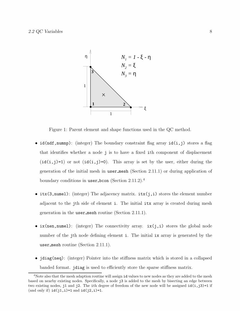
Figure 1: Parent element and shape functions used in the QC method.
• id(ndf,numnp): (integer) The boundary constraint flag array id(i,j) stores a flag
that identifies whether a node j is to have a fixed ith component of displacement
(id(i,j)=1) or not (id(i,j)=0). This array is set by the user, either during the
generation of the initial mesh in user mesh (Section 2.11.1) or during application of
boundary conditions in user bcon (Section 2.11.2).4
• itx(3,numel): (integer) The adjacency matrix. itx(j,i) stores the element number
adjacent to the jth side of element i. The initial itx array is created during mesh
generation in the user mesh routine (Section 2.11.1).
• ix(nen,numel): (integer) The connectivity array. ix(j,i) stores the global node
number of the jth node defining element i. The initial ix array is generated by the
user mesh routine (Section 2.11.1).
• jdiag(neq): (integer) Pointer into the stiffness matrix which is stored in a collapsed
banded format. jdiag is used to efficiently store the sparse stiffness matrix.
4Note also that the mesh adaption routine will assign id values to new nodes as they are added to the meshbased on nearby existing nodes. Specifically, a node j3 is added to the mesh by bisecting an edge betweentwo existing nodes, j1 and j2. The ith degree of freedom of the new node will be assigned id(i,j3)=1 if(and only if) id(j1,i)=1 and id(j2,i)=1.

2.2 QC Variables 9
• shp(nshp,numel): (double precision) Shape functions. The QC method uses three-
node linear elements, thus there is only one Gauss point at the centroid of each element.
The isoparametric formulation is used, with the parent element, local node numbering
and shape functions as shown in Fig. 1. More information on the finite element formu-
lation can be found in, for example, [12]. For each element i, the following is stored
in shp:
– shp(1,i): Derivative ∂N1/∂x.
– shp(2,i): Derivative ∂N1/∂y.
– shp(3,i): Value of N1 at the Gauss point (0.333 dp).
– shp(4,i): Derivative ∂N2/∂x.
– shp(5,i): Derivative ∂N2/∂y.
– shp(6,i): Value of N2 at the Gauss point (0.333 dp).
– shp(7,i): Derivative ∂N3/∂x.
– shp(8,i): Derivative ∂N3/∂y.
– shp(9,i): Value of N3 at the Gauss point (0.333 dp).
Here Ni(x, y) is the shape function associated with node i.
• str(nstr,numel): (double precision) Elemental stress array. str(i,j) stores the ith
component of the Kirchhoff stress5 in the jth element. Order of storage is τxx, τyy,
τzz, τxy, τxz, τyz . str is an output variable and will be updated each time the energy
or out-of-balance forces are computed for a given set of nodal displacements. The
elemental stresses are only computed in elements which touch local nodes.
• q(nq,numel): (double precision) Elemental internal variable array. q stores several
elemental quantities. For element iel:
5Note that the Kirchhoff stress τ is related to the Cauchy stress (or true stress) σ that is more commonlyused through the relation τ = Jσ, where J is the determinant of the deformation gradient F , which is storedin the internal variable array q.

2.3 Module mod boundary 10
– q(1,iel): Strain energy density.
– q(2:10,iel): Deformation gradient components in Fortran column order (F11,
F21, F31, F12, F22, F32, F13, F23, F33).
– q(11:13,iel): Eigenvalues of the right Cauchy-Green deformation tensor, C =
FTF .
– q(14,iel): Grain number containing the centroid of the element.
• x(nxdm,numnp): (double precision) The reference coordinate array. x(1..nxdm,i)
stores the reference coordinates of the ith repatom (node). Note that even though the
fields in the current QC implementation are limited to two dimensions, the x array has
three components (nxdm=3) in order to store the correct atomic crystal structure. The
initial x array is generated by the user mesh routine (Section 2.11.1).
• xsj(numel): (double precision) Elemental areas. xsj(i) stores the area (in the unde-
formed configuration) of element i.
2.3 Module mod boundary
Module mod boundary contains information and routines related to the boundaries of the
QC model. Particularly relevant for the user are the variables ncb, nce, NCEMAX and elist()
used to define outer and inner boundaries of the model that must be respected by the mesh
generation routine. The variable active() is used to define boundary segments that trigger
nonlocality. These variables are described in detail in Section 2.11.1.
2.4 Module mod grain
Module mod grain contains data and routines related to the definition and processing of
the crystallographic grains making up the system. The data in this module is not directly
accessible to the user (to prevent inadvertent errors being introduced). However, a series
of routines have been defined to allow a user to query the values of variables stored there.
2.4 Module mod grain 11
Some of these variables can be very useful for generating the initial arrangement of nodes
in user mesh. This is discussed further in Section 2.11.1. See also Section 3.5 of the QC
Tutorial Guide where the grain definition and associated variables are defined. The data
query routines in mod grain are:
• NumGrains: number of grains
• GetGrainCellSize: repeating cell dimensions for a given grain
• GetGrainNumCell: number of atoms in the repeating cell for a given grain
• GetGrainCellAtom: coordinates of a given atom in the repeating cell for a given grain
• GetGrainBvec: Bravais vector matrix for a given grain
• GetGrainBinv: inverse Bravais vector matrix for a given grain
• GetGrainRefStiff: reference stiffness matrix for a given grain
• GetGrainRefatom: reference atom for a given grain
• GetGrainSpecies: atomic species for a given grain
• GetGrainNumVrts: number of vertices for polygon of a given grain
• GetGrainVertex : given vertex of the polygon of a given grain
• GetGrainXlatvect: crystallographic axes for a given grain
Another useful routine in mod grain is NearestBSite that returns the nearest Bravais site
to a given point. This routine is used to ensure the requirement normally imposed in QC
that nodes must occupy lattice sites in the reference configuration. The use of this routine
and its calling format are discussed in Section 2.11.1.

2.5 Module mod mesh 12
2.5 Module mod mesh
Module mod mesh contains routines related to the generation of two-dimensional triangular
meshes. This module is built around contri, a constrained Delaunay triangulation program
developed by Sloan [13, 14]. Two routines in mod mesh are accessed by users:
• delaunay: the main triangulation routine that calls contri. This routine is discussed
in Section 2.11.1.
• PerturbMesh: a routine for slightly perturbing (or unperturbing) the nodes in a mesh
prior to (or after) triangulation to obtain uniform or symmetric meshes. This is dis-
cussed in Section 2.11.1.
2.6 Module mod output
Module mod output provides a standardized interface for generating output in QC. Rather
than printing directly to the output stream, a set of routines and associated variables are
provided that allow the user to generate output in the user routines consistent with the
QC format. This includes an indentation hierarchy that positions the output in way that
makes reading output files much easier. The output interface has three main components
for generating (1) standard output, (2) error messages, and (3) log file entries.
1. To generate standard output, the desired output is stored in the character(len=160)
variable string and then a call output statement is issued. For example,
string = ’Message from the user!’call output
will print the text “Message from the user!” in the appropriate place in the QC output
file. Variable data can be printed in the following manner:
write(string,’(a,i5)’)’**numnp = ’,numnpcall output

2.6 Module mod output 13
The write statement places the formatted output in string, which is then sent to the
output file by call output.
2. To generate an error message, the nerror lines of the message are stored in the
character(len=160) array error(nerrmax). Note that nerror must be less than
the maximum allowed value nerrmax (currently set to 25). The output is generated
by issuing a call erroroutput statement. Typically this statement is followed by a
stop statement to terminate program execution. For example,
if (kount > maxnp) thennerror = 2error(1) =
& ’Number of nodes exceeds maxnp in subroutine user_mesh’write(error(2),’(a,i5)’)’**maxnp = ’,maxnpcall erroroutputstop
endif
This code segment from a user mesh routine checks whether the number of nodes
generated by the meshing routine (given by kount) exceeds the maximum allowed value
of maxnp. If it does, an appropriate error message is issued and execution terminates.
The call erroroutput statement will send the error message to the output file and
will also generate a log entry in the log file. As for standard output, variable data can
be stored in error() lines using write statements.
3. The log file qc.log is used to output large amounts of data that would clutter up
the standard output file. To generate a log file entry, the desired output is stored in
the character(len=160) variable string and then a call logoutput statement is
issued. For example,
! Check for repeating nodesdo i = 1, numnp
do j = i+1, numnpif ( abs(x(1,i)-x(1,j)) < tol .and.
& abs(x(2,i)-x(2,j)) < tol ) thennerror = 2write(error(1),’(a,i5,a,i5)’)’Node’,j,’ coincides with’,i
2.6 Module mod output 14
error(2) =& ’Node list sent to log file (subroutine user_mesh)’
call erroroutput! list nodes to log filestring = ’Node List:’; call logoutputstring = ’ node x y ’call logoutputdo k=1,numnp
write(string,’(i5,2x,f12.5,2x,f12.5)’)k,x(1:2,k)call logoutput
enddostop
endifenddo
enddo
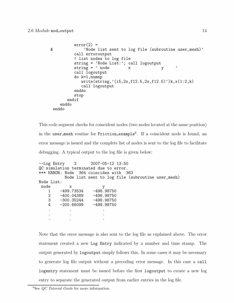
This code segment checks for coincident nodes (two nodes located at the same position)
in the user mesh routine for Friction example6. If a coincident node is found, an
error message is issued and the complete list of nodes is sent to the log file to facilitate
debugging. A typical output to the log file is given below:
--Log Entry 2 2007-05-12 13:50QC simulation terminated due to error.*** ERROR: Node 364 coincides with 363
Node list sent to log file (subroutine user_mesh)Node List:node x y
1 -499.73534 -498.987502 -400.04389 -498.987503 -300.35244 -498.987504 -200.66099 -498.98750. . .. . .. . .
Note that the error message is also sent to the log file as explained above. The error
statement created a new Log Entry indicated by a number and time stamp. The
output generated by logoutput simply follows this. In some cases it may be necessary
to generate log file output without a preceding error message. In this case a call
logentry statement must be issued before the first logoutput to create a new log
entry to separate the generated output from earlier entries in the log file.
6See QC Tutorial Guide for more information.

2.7 Module mod pload 15
2.7 Module mod pload
Module mod pload provides access to variables and routines related to the proportional
loading table and time7 management. The data in this module is not directly accessible to
the user (to prevent inadvertent errors being introduced). However, a series of routines have
been defined to allow a user to query the values of variables stored there. Some of these
variables can be necessary to the user when applying boundary conditions. See Section 2.11.2
for a discussion of how boundary conditions are applied in QC. The data query routines in
mod pload are:
• GetLoadTime: current loading time (time)
• GetLoadTimeStep: current loading timestep (dt)
• GetLoadPropFact: current loading proportional factor (prop)
• GetLoadOldPropFact: previous loading proportional factor (propol)
• TimeStepMax: compute the maximum possible time step that after the application of
boundary conditions will just result in a node being pushed onto the opposite element
side, i.e. that will cause element warping.
• PropToTime: given a current time and a desired property value, returns the required
future time.
See module mod pload for details on the calling format for these routines. Some examples
of their use are given below in Section 2.11.2.
2.8 Module mod qclib
Module mod qclib is a library of general-purpose routines used by other modules in QC.
There are a variety of vector and matrix manipulation routines, geometric routines, character
7This version of QC is a static zero temperature implementation. “time” refers to an arbitrary load stepcounter and not an actual measure of time.

2.9 Module mod repatom 16
string manipulation routines, and miscellaneous routines (such as a pseudo random number
generator). Details of these routines are given in mod qclib and will not be reproduced here,
except for three routines that are particularly important for the user programs. The first
two are routines used to parse input lines from the input file:
• next: integer function to find the next delimiter (comma or space) in a string.
• freein: subroutine to parse free-form input lines.
These two commands work in tandem to extract variables from the comma delimited vari-
ables on QC input lines. Examples of how these routines are used are given in Sections 2.11.1
and 2.11.2.
The third useful routine in mod qclib is qsortr. This routine sorts the first column
of a list containing two columns and n rows according to a key variable xkey. The sort-
ing direction is determined by the variable sign (= 1.0 for ascending sort, = −1.0 for
descending sort). For an ascending sort, upon return from qsortr all elements satisfy:
xkey(list(1,i)) ≤ xkey(list(1,i+1)). The calling format is:
call qsortr(n,list,xkey,sign,listdim,keydim)
Here listdim is the allocated dimension of list (n ≤ listdim) and keydim is the allocated
dimension of xkey (keydim ≥ max{list(1,1:n)}). This routine is used in user mesh to sort
the nodes defining outer and inner boundaries (i.e holes) in the model in counter-clockwise
and clockwise directions, respectively. See Section 2.11.1 for more information on this.
2.9 Module mod repatom
Module mod repatom is one of the main modules in the QC code dealing with many aspects
of the definition and processing of representative atoms. Users should not need to directly
access variables in this module. The exception is the logical array protected() that allows
a user to mark certain representative atoms as permanent, i.e. ones that cannot be deleted

2.10 Module mod stiff 17
by the adaption routine during its coarsening phase. For example, to protect node i from
deletion set
protected(i) = .true.
in user mesh. Normally the reason for doing this is to maintain a “skeleton” of the model
even if the coarsening algorithm determines that most nodes are not necessary. It is also
possible to set protected from the input file. This is discussed in Section 4.16.
2.10 Module mod stiff
Module mod stiff is used to store the tangential stiffness matrix tang. To minimize storage
requirements the symmetric banded nature of the stiffness matrix is exploited. Only the main
diagonal of the stiffness matrix and columns of numbers above the diagonal that terminate
in a non-zero element are stored. This list of numbers is stored in concatenated form in tang
with the associated vector jdiag(i) pointing to the position of the (i,i)-th element of the
stiffness matrix. A function istiff that is also located in mod stiff returns the index into
tang for a specific element. See Section 2.11.4 for an example how these variables are used.
2.11 User-Specified Routines
As noted above the user must supply QC with a user APP.f containing five routines. At
the top of this file is a module mod uservars that can be used by the user to pass variables
between the different user routines. For reasons of downward compatibility the module
always contains the following two arrays:8
• user iparam(10) (Integer): Array of integers available for storage of user-specific
parameters to pass information between the user routines. See Section 2.11.1.
• user rparam(10) (Real): Same as above for real (double precision) variables.
8In earlier versions of QC these variables were stored in module mod global.

2.11.1 user mesh 18
See Section 2.11.4 for an example how module uservars is used. The required user routines
are described in the following sections.
Note: In order to facilitate the porting of user mesh, user bcon and user pdel routines
from earlier versions of QC (where they were stored in separate files), a user template.f
file is supplied with the distribution code in the QC directory. This file is complete except for
blank places left for these routines along with helpful instructions on the changes that must
be introduced to port over old files.
2.11.1 user mesh
Other than the mesh generators provided with specific examples in the QC package, there
are no mesh-generating capabilities in QC. Instead, the user is required to write a mesh
generating routine user mesh and compile and link it with the main QC routines. QC does
include a number of tools, most notably a constrained Delaunay triangulation routine [13],
that facilitate mesh generation. These tools are described below.
The user mesh routine is initiated by a mesh statement in the head stage of the input
file (see Section 3.7). The calling format for this macro is
mesh[,key][,data]
where key and data are problem-specific data that are passed to user mesh as explained
below. In addition, the lines immediately following the mesh command in the input file can
be read by this routine to provide additional input to the mesh generator. See below under
the heading “Direct input to the user mesh routine” for more information on this.
The header of a typical user mesh subroutine is as follows:
subroutine user_mesh(id,x,ix,f,b,itx,key,input)use mod_uservarsuse mod_global, only : dp,maxel,maxnp,ndf,ndm,nen,numel,numnp,
& nxdmuse mod_output, only : erroroutput,nerror,output,string,erroruse mod_boundary, only : ncb,nce,NCEMAX,elistuse mod_repatom, only : protecteduse mod_qclib, only : next,freein,qsortr

2.11.1 user mesh 19
use mod_mesh, only : delaunay,PerturbMeshuse mod_grain, only : NumGrains,GetGrainNumVrts,GetGrainVertex,
& NearestBSiteimplicit none
!-- Transferred variablesinteger, intent(inout) :: id(ndf,maxnp),
& ix(nen,maxel),& itx(3,maxel)real(kind=dp), intent(inout) :: x(nxdm,maxnp),
& f(ndf,maxnp),& b(ndf,maxnp)character(len=4), intent(in) :: keycharacter(len=80), intent(in) :: input
The header begins with a list of modules used by user mesh. Note the use of the only clause
for all modules indicating the specific variables and routines accessed from the module. This
is good programming practice, both from a readability standpoint and as an aid to the
compiler to detect errors. The important variables and routines in these module are described
in Section 2.1, and Sections 2.3 to 2.9. More details are also available in the comments at
the top of the module files.
Variables pass to user mesh. The variables passed to user mesh (except for key and
input are described in Section 2.2. Here a brief definition is given with additional comments
specific to the user mesh routine.
• id(ndf,numnp): (integer) The boundary constraint flag array. This array can be
initialized either here in user mesh or in user bcon.
• x(nxdm,numnp): (double precision) The reference coordinate array. The initial x array
must be generated here by the user mesh routine. Details and useful tools are discussed
below.
• ix(nen,numel): (integer) The connectivity array. The initial ix array must be gener-
ated here by the user mesh routine. Details and useful tools are discussed below.
• f(ndf,numnp): (double precision) The boundary condition array. This array can be
initialized either here in user mesh or in user bcon.

2.11.1 user mesh 20
• b(ndf,numnp): (double precision) Nodal Displacement Array. This array can be ini-
tialized here in user mesh or in user bcon if desired. (By default it is initialized to
zero at the start of the simulation.)
• itx(3,numel): (integer) The adjacency matrix. The initial itx array must be gener-
ated here by the user mesh routine. Details and useful tools are discussed below.
• key: (character(len=4)) Key passed from the input file command line. Can be used to
implement various options in the mesh generator. By convention, key=’dire’ indicates
that additional input to user mesh follows the mesh command line. See below under the
heading “Direct input to the user mesh routine”. Note that this variable should
not be modified by the user mesh routine.
• input: (character(len=80)) Input data passed from the input file command line. input
can be used to pass character, double precision, integer or logical data directly from
the command line to the user mesh routine. It is left to the user to parse this data.
Routines in mod qclib (see Section 2.8) facilitate this as shown below. Note that
this variable should not be modified by the user mesh routine.
As an example of how the input variable can be parsed, consider the user mesh routine for
GB example9. This routine defines the following calling format for the input file:
mesh,,nx,ny
where nx and ny are the number of divisions along the x and y axes. Everything beyond
the second comma will be passed to the user mesh subroutine in the variable input. For
example, if the input file contains
mesh,,8,8
the variable input passed to user mesh contains ‘8,8’. The following code segment in
user mesh parses this input into the variables nx and ny:
9See QC Tutorial Guide for more information.

2.11.1 user mesh 21
integer lower,upper,nx,nyreal(kind=dp) dum...! Parse inputlower = 0upper = next(lower,input)call freein(input,lower,upper,nx,dum,1)lower = upperupper = next(lower,input)call freein(input,lower,upper,ny,dum,1)
The function next simply starts from the integer position lower in the string input, and
returns the position of the next ‘,’ or end-of-line character in the string. The routine
freein parses a string between positions lower+1 and upper-1 as either an integer if the
last variable in the list is ‘1’ or a double precision real is the last variable in the list is
‘2’. If the return value is to be an integer, it is returned in the fourth variable on the
list (‘nx’ or ‘ny’ in this case), while a double precision return value is returned in the
fifth variable. Another example of a code segment parsing input that also reads in double
precision variables is given in Section 2.11.2.
Note that the text-parser routine freein expects the characters between each pair of
commas (i.e. from lower+1 to upper-1) to be consistent with integer or double precision
formatting. For example, no letters (a-z) should appear in an integer field.
Expected output from the user mesh routine. The user-routine for mesh generation
must define the following variables:
• numnp: (integer). The number of repatoms in the mesh. This is a global variable in
mod global.
• numel: (integer). The number of elements in the mesh. This is a global variable in
mod global.
• ix: (integer). The connectivity matrix, as described above. Note that the constrained
Delaunay triangulator that is provided with QC is a great help in generating this

2.11.1 user mesh 22
matrix. How to use this triangulator is described under the heading “Constrained
Delaunay triangulation” below.
• itx: (integer). The adjacency matrix, as described above. Note that the constrained
Delaunay triangulator that is provided with QC is a great help in generating this
matrix. How to use this triangulator is described under the heading “Constrained
Delaunay triangulation” below.
• nregion: (integer). It is possible to define a model with several separately meshed
regions. For example, in a nano-indentation simulation, one may wish to mesh the
indenter separately from the indented substrate. The global variable nregion is found
in the mod global module, and must be defined to be the number of regions. The
default value is set to nregion=1, so for a simple mesh with one region, nothing needs
to be done in the user mesh routine.
Note that modeling contact problems between two regions requires some care. QC will
only reliably detect contact between two nonlocal regions, so the surfaces expected to
come into contact must be made nonlocal.
• iregion(numnp): (integer). Related to the nregion variable described above, this
array assigns each repatom in the problem to one of the regions to be meshed. Thus
iregion(i) is the region to which repatom i belongs. The default value is set to
iregion(i)=1 for all i, so for a simple mesh with one region, nothing needs to be
done in the user mesh routine. Once nregion and iregion is set in user mesh, it will
be kept up to date by the code automatically during subsequent mesh adaption.
• x: (double precision). The reference coordinates of all repatoms, as discussed in the
list of input variables above. Note that the QC normally requires repatoms to lie on
Bravais lattice sites. The requirement is only relaxed for a fully local QC simulation,
in which case the user can set choose to set NodesOnBSites=.false. (see the flag
command). Two items available to the user mesh routine simplify the generation of

2.11.1 user mesh 23
conforming points. First, there is a subroutine NearestBsite which, given a point in
the simulation plane, returns the nearest Bravais site. (See Section 2.4). Its header is
as follows:
subroutine NearestBSite(u,CheckModel,xa,igrain,iel,x,b,ix,itx)use mod_global, only : dp,maxel,maxnp,ndf,ndm,nen,nxdm,NodesOnBsitesimplicit none
!-- Transferred variablesreal(kind=dp) u(ndm), xa(3),x(nxdm,maxnp),b(ndf,maxnp)integer igrain,iel,ix(nen,maxel),itx(3,maxel)Logical CheckModel
The variables x, b, ix, itx are as previously defined and are not modified by the
routine. The others are:
– u(ndm): (double precision, in). Coordinates of the point. In the 2D QC imple-
mentation, ndm=2.
– CheckModel: (logical, in). If CheckModel=.true., the routine will return the
closest point that is inside the current model boundaries, otherwise it will not
check whether the new point lies in the model. In the user mesh routine, the
model is in the process of being defined and therefore this flag is typically .false..
Note that if CheckModel=.false. then the variables iel,x,b,ix,itx are not
used by the NearestBSite routine. Thus, dummy arguments can be passed to
the subroutine in this case, which is important when NearestBSite is being used
during initial mesh generation.
– xa(nxdm): (double precision, out), Returned coordinates of the Bravais site.
– igrain: (integer, out), Returned grain number in which the site resides.
– iel: (integer, in/out) : If checkmodel is .true., iel returns the element in
which the returned point sits. Also, iel is used as the element from which to
start searching (breadth-first search) to determine if the point is in the model. It
can be initialized to 0 if an intelligent guess for a starting point is not known.

2.11.1 user mesh 24
The second item that is useful for generating a set of nodes x that are on lattice sites
is the periodic cell for each grain, as discussed in Section 3.5 of the QC Tutorial
Guide. This cell is useful because it can be used to “tile” the model with all the possible
lattice sites in space for the given orientation of the grains. This tiling can serve as a
template for choosing a sensible location for each repatom in the mesh. The following
code segments use the routines described in Section 2.4 to extract the cell variables for
grain igrain:
– The number of atom sites in the cell ncell:
integer ncellcall GetGrainNumCell(igrain,ncell)
– The coordinates of the atoms in the cell. cellatom(1:3) contains the coordinates
of the jth atom (j ≤ ncell):
real(kind=dp) cellatom(3)call GetGrainCellAtom(igrain,j,cellatom)
– The periodic lengths of the cell dcell(3) in the three coordinate directions:
real(kind=dp) dcell(3)call GetGrainCellSize(igrain,dcell)
Constrained Delaunay triangulation. Relatively speaking, the selection of a set of
repatoms is a simple task while correctly generating a mesh of these points (i.e. generating
connectivity and adjacency matrices) can be difficult. Therefore, QC includes a constrained
Delaunay triangulator called contri [13, 14]. To use contri, the user needs only to define the
coordinates of all the repatoms in the problem. If the mesh is relatively simple (specifically if
it is a simply-connected convex hull) no more information is needed. For multiply-connected
regions (i.e. with holes) or non-convex outer boundaries, the user must also generate a set
of constrained edges and boundaries for the mesh.
A boundary is made up of a series of edges, each of which is defined by the repatoms at
the start and end of the edge. The edges that define the boundaries may be listed in any

2.11.1 user mesh 25
order, but the repatoms defining external boundary edges must be listed counter-clockwise
around the boundary, while edges for internal boundaries (holes) must be listed clockwise. In
addition to boundaries, internal edges can also be specified to insure that these edges appear
in the final mesh. For example, it may be desirable that the path of a grain boundary is
closely followed by the edges of the elements in a bi-crystal simulation.
Constrained boundary and edge information is stored in mod boundary. (See Section 2.3.)
The information that the user must generate before calling the triangulator is as follows:10
• nce: (integer). The number of constrained edges. For convex hull triangulation, nce=0
• ncb: (integer). The number of constrained boundary edges. For convex hull triangu-
lation, ncb=0. Note that nce must be greater than or equal to ncb.
• elist(2,nce): (integer). The repatom numbers defining each edge. Constrained
boundary edges must appear in the list before any internal constrained edges. Each
edge i goes from repatom elist(1,i) to elist(2,i). As mentioned earlier, boundary
edges can appear in any order but must be listed in their counter-clockwise sense if
they are external boundaries and in their clockwise sense if they are internal boundaries
(holes). There are different ways for ensuring this. One approach that uses the routine
qsortr described in Section 2.8 is to identify all of the nodes on a boundary, sort
them in counter-clockwise fashion (for an outer boundary) and then defined the edges
by connecting the nodes in series. A code segment that does this, taken from the
GB example11, is given below:
real(kind=dp), allocatable :: vtmp(:)real(kind=dp) xmin,xmax,ymin,ymax,xx,yy,xc,ycinteger i...! Identify nodes lying on the boundaries and sort! in counterclockwise fashion for constrained Delaunay algorithm
10See also the discussion under the heading “The model boundary” below.11See QC Tutorial Guide for more information.

2.11.1 user mesh 26
1 xmax=xmax-0.2_dp*dx2 xmin=xmin+0.2_dp*dx3 ymax=ymax-0.2_dp*dy4 ymin=ymin+0.2_dp*dy5 nce = 06 allocate(vtmp(numnp))7 do i=1,numnp8 xx=x(1,i)9 yy=x(2,i)10 if (xx.lt.xmin .or. xx.gt.xmax .or.
& yy.lt.ymin .or. yy.gt.ymax) then11 nce=nce+112 if (nce.gt.NCEMAX) then13 nerror = 114 error(1) = ’nce exceeds NCEMAX in subroutine user_mesh’15 call erroroutput16 stop17 endif18 elist(1,nce)=i19 vtmp(i)=datan2(yy-yc,xx-xc)20 endif21 enddo22 call qsortr(nce,elist,vtmp,1.0_dp,NCEMAX,numnp)23 deallocate(vtmp)
! Finish defining boundary24 elist(2,nce)=elist(1,1)25 ncb = nce26 do i=1,nce-127 elist(2,i)=elist(1,i+1)28 enddo
The domain to be meshed in this case is a simple rectangle with minimum and maxi-
mum dimensions in the x and y directions, xmin, xmax, ymin, and ymax. The spacing
between nodes is dx and dy, so lines 1–4 ensure that the test in line 10 is true for any
nodes lying on the outer boundary (the perimeter of the rectangle). The nodes on the
boundary are added to elist in line 18. For each node i on the boundary, vtmp(i)
computed in line 19, contains the angle to this point from the center of the rectangle
(xc,yc). The boundary nodes are sorted in counter-clockwise order in line 22 using
the routine qsortr. The boundary list is completed in lines 24–27. Note that since
a rectangle is a convex region, the entire procedure of identifying the nodes on the
boundary and sorting them is unnecessary. The default behavior of contri with no
boundary defined would have given the same result. This is only done in this routine

2.11.1 user mesh 27
as an example.
Once these data are generated (normally within the user mesh) routine, the triangulator
is executed. In QC, this is done by calling the subroutine delaunay with the following
header:
subroutine delaunay(x,ix,b,f,id,itx)use mod_global, only : dp,iregion,maxel,maxnp,ndf,nen,neq,
& nregion,numel,numelast,numnp,nxdm,NeedItxuse mod_output, only : erroroutput,nerror,output,string,erroruse mod_boundary, only : IncreaseElist,nce,ncb,elist,active,NCEMAXimplicit none
!-- Transferred variablesinteger, intent(inout) :: ix(nen,maxel)integer, intent(inout) :: id(ndf,maxnp)real(kind=dp), intent(inout) :: x(nxdm,maxnp),b(ndf,maxnp),
& f(ndf,maxnp)integer, intent(out) :: itx(3,maxel)
where x, ix, b and itx are as previously defined. If the global logical variable DefMesh
is .false. (the default), the mesh is generated using the reference configuration of points
(x), otherwise the deformed configuration is used (x+b). Upon successful completion of this
routine, the matrices ix and itx will be defined.
Symmetric and regular mesh generation. It is often desirable that the orientation of
the triangular elements in a finite element mesh be as regular12 or symmetric as possible.
The QC program includes a utility routine that can be used by the user mesh routine to
generate regular or symmetric meshes.
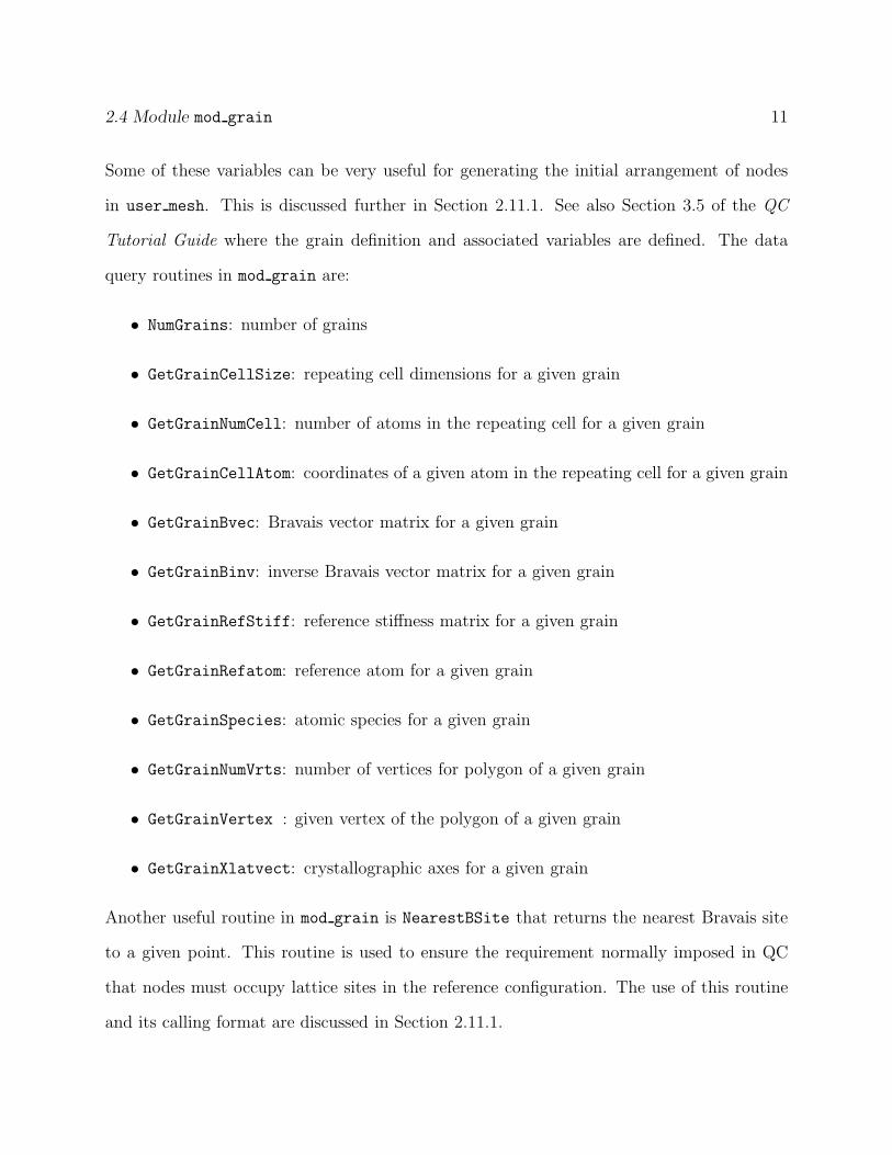
The Delaunay triangulation algorithm can be coaxed into producing a regular or sym-
metric mesh by introducing a bias in the nodal locations prior to calling the meshing routine.
For example, a regular square array of nodal points will be meshed with randomly oriented
triangles depending on the numerical precision to which the nodal coordinates are speci-
fied (see Fig. 2(a)). On the other hand, if the square array is slightly sheared so that the
squares become parallelograms, the mesh will become perfectly regular (see Fig. 2(b)). If
12Here regular means that all elements are oriented in the same direction.

2.11.1 user mesh 28
-500 0 500-1000
-800
-600
-400
-200
0
-500 0 500-1000
-800
-600
-400
-200
0
-500 0 500-1000
-800
-600
-400
-200
0
(a) (b) (c)
Figure 2: Three uniform meshes obtained from delaunay depending on whetherPerturbMesh was called and the setting of SymmetricMesh. (a) Random mesh(PerturbMesh not called, SymmetricMesh=.false.), (b) Regular mesh (PerturbMeshcalled, SymmetricMesh=.false.), (c) Symmetric mesh (PerturbMesh called,SymmetricMesh=.true. with SymmetryDof = 1 and SymmetryValue = 0.0 dp).
the perturbation is selected in a symmetric manner, a symmetric mesh can be obtained (see
Fig. 2(c)).
The QC program provides a utility routine PerturbMesh and several global variables
(SymmetricMesh, SymmetryDof, SymmetryValue) that control the mesh morphology. The
Perturbmesh subroutine header is as follows:
subroutine PerturbMesh(x,perturb)use mod_global, only : dp,nxdm,maxnp,numnp,
& SymmetricMesh,SymmetryDof,SymmetryValueimplicit none
!--Transferred variableslogical, intent(in) :: perturbreal(kind=dp), intent(inout) :: x(nxdm,maxnp)
where x is as previously defined and perturb is a logical flag. When perturb=.true.,
the nodal coordinates are modified to produce a bias for the Delaunay algorithm. When
perturb=.false., the opposite bias is applied, canceling the effect of the previous pertur-
bation.
Code segments that produce random, regular and symmetric meshes are shown below.
A random mesh (Fig. 2(a)) is the default behavior obtained from simply calling delaunay:
call delaunay(x,ix,b,f,id,itx)
A regular mesh (Fig. 2(b)) is obtained by applying PerturbMesh with symmetry off:

2.11.1 user mesh 29
SymmetricMesh=.false.call PerturbMesh(x,.true.)call delaunay(x,ix,b,f,id,itx)call PerturbMesh(x,.false.)
A symmetric mesh (Fig. 2(c)) is obtained by applying PerturbMesh with symmetry on:
SymmetricMesh=.true.SymmetryDof=1SymmetryValue=0.0_dpcall PerturbMesh(x,.true.)call delaunay(x,ix,b,f,id,itx)call PerturbMesh(x,.false.)
Here, the first three lines are global variables (found in the module mod global) provided to
the PerturbMesh routine. SymmetricMesh is a logical flag set to true if the symmetric mesh
option is desired. SymmetryDof is an integer that defines the coordinate (1=x or 2=y) used
to define the plane of symmetry and SymmetryValue is a double-precision value defining the
coordinate of the plane of symmetry. The call to PerturbMesh modifies the x values prior
to the call to delaunay, which produces the mesh. Finally, the second call to PerturbMesh
restores the correct values in x. In this example, the nodal points are temporarily sheared
in such a way as to make the elements appear symmetrical about the plane x=0.0 dp.
It is important to note that regular (or symmetric) meshes can only be obtained if the
nodes themselves are regular (or symmetric). Due to the constraint that nodes must lie on
lattice sites, sometimes even arrangements of nodes that appear regular (or symmetric) are
not exactly so as a result of small adjustments to the positions of nodes. To prevent this
problem, nodes for regular (or symmetric) meshes, should be generated to be consistent with
the underlying lattice structure from the start by using the grain repeating cell information
as explained above.
The model boundary. The definition of the mesh, and more specifically the assignment
of the variables ncb, nce, and elist described above also defines the spatial extent of the
model. Prior to the assignment of these variables by the user mesh routine, there is only the
definition of the regions containing each grain as defined by the grain command. The QC

2.11.1 user mesh 30
program does not require that the grain shapes match the mesh shape, but every element
must lie inside one or more grains. Thus, it is often convenient to define grains that are much
larger than the intended region to be modeled, allowing the user mesh routine to effectively
“cut out” a region of this space to define the actual model.
Once the mesh is defined, the list of boundary edges contained in elist defines the true
boundary of the model. This has ramifications for mesh adaption, as any repatoms added
during adaption will lie inside this model boundary.
The model boundary is also used by the QC to determine the location of free surfaces.
Specifically, each boundary segment j stored in the array elist is also associated with a
logical variable active(j) found in the module mod boundary. It is left to the user, during
the execution of the user mesh routine, to define the active variable for each boundary
segment. If a segment of the boundary is “active” (i.e. active(j)=.true.), this free
surface will trigger a region of nonlocality within a distance PROXFACT*rcut. Thus, the
model will automatically refine the mesh in this region down to the atomic scale and make
every repatom in the region nonlocal. Also see Sections 3.3 and 3.4 for discussions of the
model parameters PROXFACT and SurfOn.
Regions of the model where boundaries are set to be inactive (active(j)=.false.) will
not correctly include surface energetics, but can significantly reduce the computational effort
where these energetics are not expected to have an important effect on the phenomena of
interest. For example, in studying crack tip phenomena, it is sensible to include the surface
effects only for a short distance along the crack faces near the tip, turning the surfaces off
for the majority of the traction free crack faces.
If the user’s mesh is a simply-connected convex region, the constrained Delaunay routine
does not need any defined boundaries to produce the correct mesh of the points. In this
case, the variables nce, ncb and elist are assigned automatically by the program during
the Delaunay triangulation so that the correct model boundary is stored. In this case,
all model boundaries are set to be inactive (active(j)=.false.) unless the user specifies

2.11.1 user mesh 31
otherwise following the call to the Delaunay triangulator.
Optional output from the user mesh routine. The user may choose to define the
variables f and id either during mesh generation, or during the application of the boundary
conditions in the user bcon routine. See Section 2.11.2 for an explanation how boundary
conditions are applied in QC.
It is sometimes convenient to pass mesh-specific information to the boundary condition
routine (user bcon, see Section 2.11.2) that can only be determined at the time of mesh
generation. To facilitate this passage of information, module uservars is included in the
user APP.f file. As noted earlier, to be compatible with earlier versions of QC it contains
by default the following two variables:13
• user iparam(10): (integer). Storage for up to 10 integer parameters.
• user iparam(10): (double precision). Storage for up to 10 double precision parame-
ters.
Since both the user mesh and user bcon routines use the mod uservars module, param-
eters stored in these variables during the execution of user mesh will be accessible to the
user bcon routine later in the simulation.
Direct input to the user mesh routine. Additional input for the meshing routine can be
listed in the lines immediately following the mesh command in the input file. By convention,
if this is the case, no input should be given on the command line itself and key should be set
to ’dire’. The additional input is read in from the input stream in the user mesh routine
using Fortran read statements:
read(cmdunit,format-spec) list
where cmdunit is the file handle for the input stream (a global QC variable defined in
mod global), format-spec is the format specifier (use * for unformatted input), and list is the
13Of course the user may opt to add on any additional variables.

2.11.2 user bcon 32
list of data variables to be read in. For example to read in two integers nx and ny, indicating
perhaps the number of divisions along the x and y directions, the following statement could
be used:
read(cmdunit,*) nx,ny
Each read statement corresponds to one line following the mesh command and as many read
statements as wanted can be used.
2.11.2 user bcon
The user bcon routine is called by macro bcon (see Section 4.2) to apply special bound-
ary conditions to the simulation. Before this routine can be discussed it is necessary to
explain how boundary conditions are applied in QC. Two variables in QC are related to the
application of boundary conditions:
• time: (double precision) A scalar measure of the load step. Despite its name, this is
a dimensionless variable that merely serves as a load step counter. It is increment by
macro time that is discussed in Section 4.25.
• prop: (double precision) The value corresponding to time in the proportional load
table (see Section 4.15). This table is a graph relating time to a physical property
prop that is used to defined the boundary conditions. For example, prop could be
the vertical displacement of an indenter in a nanoindentation simulation, the stress
intensity factor in a fracture simulation, the shear strain in a shearing test, etc.
QC automatically uses prop to apply boundary conditions at each load step. Just prior to
invoking the solver, the QC program executes two code segments to assign displacements to
constrained degrees of freedom and external forces to free degrees of freedom:
! Set displacements of constrained nodesdo i=1,numnp
do j=1,ndfif (id(j,i)==1) b(j,i) = prop*f(j,i)
enddo
2.11.2 user bcon 33
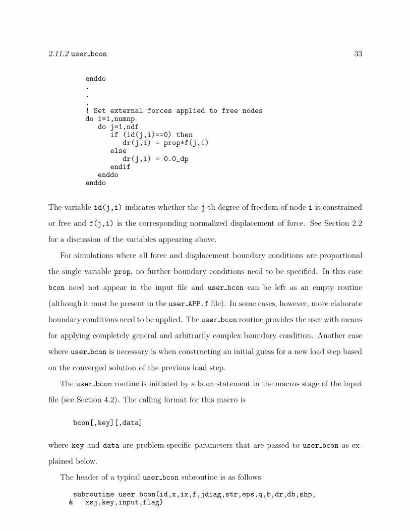
enddo...! Set external forces applied to free nodesdo i=1,numnp
do j=1,ndfif (id(j,i)==0) then
dr(j,i) = prop*f(j,i)else
dr(j,i) = 0.0_dpendif
enddoenddo
The variable id(j,i) indicates whether the j-th degree of freedom of node i is constrained
or free and f(j,i) is the corresponding normalized displacement of force. See Section 2.2
for a discussion of the variables appearing above.
For simulations where all force and displacement boundary conditions are proportional
the single variable prop, no further boundary conditions need to be specified. In this case
bcon need not appear in the input file and user bcon can be left as an empty routine
(although it must be present in the user APP.f file). In some cases, however, more elaborate
boundary conditions need to be applied. The user bcon routine provides the user with means
for applying completely general and arbitrarily complex boundary condition. Another case
where user bcon is necessary is when constructing an initial guess for a new load step based
on the converged solution of the previous load step.
The user bcon routine is initiated by a bcon statement in the macros stage of the input
file (see Section 4.2). The calling format for this macro is
bcon[,key][,data]
where key and data are problem-specific parameters that are passed to user bcon as ex-
plained below.
The header of a typical user bcon subroutine is as follows:
subroutine user_bcon(id,x,ix,f,jdiag,str,eps,q,b,dr,db,shp,& xsj,key,input,flag)

2.11.2 user bcon 34
use mod_uservarsuse mod_global, only : dp,maxel,maxneq,maxnp,ndf,ndm,nen,nq,nstr,
& numnp,nxdmuse mod_output, only : output,stringuse mod_pload, only : GetLoadPropFact,GetLoadOldPropFact,
& GetLoadTime,GetLoadTimeStepimplicit none
!-- Transferred variablesreal(kind=dp), intent(inout) :: b(ndf,maxnp),str(nstr,maxel),
& eps(nstr,maxel),q(nq,maxel),& x(nxdm,maxnp),f(ndf,maxnp),& dr(ndf,maxnp),db(maxneq),& shp(3,nen,maxel),xsj(maxel)integer, intent(inout) :: jdiag(maxneq),ix(nen,maxel),
& id(ndf,maxnp)character(len=80), intent(in) :: inputcharacter(len=4), intent(in) :: keylogical, intent(inout) :: flag
The header begins with a list of modules used by user bcon. The use of the only clause
is encouraged as a good programming practice (see Section 2.11.1 for more on this). The
important variables and routines in these module are described in Section 2.1, 2.6 and 2.7.
More details are also available in the comments at the top of the module files.
The variables passed to user bcon (except for key, input and flag) are described in Sec-
tion 2.2. Here a brief definition is given with additional comments specific to the user bcon
routine including details on how user bcon normally operates on these variables.
• id(ndf,numnp): (integer) The boundary constraint flag array. This array is set by the
user, either during the generation of the initial mesh in user mesh (Section 2.11.1) or
here in the user bcon routine.
• x(nxdm,numnp): (double precision) The reference coordinate array. Note that the x
array should not be modified by the user bcon routine.
• ix(nen,numel): (integer) The connectivity array. Note that the ix array should
not be modified by the user bcon routine.
• f(ndf,numnp): (double precision) The boundary condition array. This array is set by
the user, either during the generation of the initial mesh in user mesh (Section 2.11.1)

2.11.2 user bcon 35
or here in the user bcon routine.
• jdiag(neq): (integer) Pointer into the stiffness matrix which is stored in a col-
lapsed banded format. Note that this variable should not be modified by
the user bcon routine.
• str(nstr,numel): (double precision) Elemental Stress array. This variable may be
useful for an application where the applied boundary conditions vary in response to
the stress in the material. Note that this variable should not be modified by
the user bcon routine.
• eps(nstr,numel): (double precision) Elemental strain array. This variable may be
useful for an application where the applied boundary conditions vary in response to
the strain in the material. Note that this variable should not be modified by
the user bcon routine.
• q(nq,numel): (double precision) Elemental internal variable array. Note that this
variable should not be modified by the user bcon routine.
• b(ndf,numnp): (double precision) Nodal Displacement Array. This variable is typically
modified in the user bcon routine as a means of applying an initial guess to the solution
of the nonlinear problem at hand. Judicious initial guesses to the equilibrium solution
can significantly enhance convergence rates and prevent nonphysical energy minima
from being reached by the nonlinear solver.
Depending on the problem, the initial guess may simply be the solution field from the
previous load step, or that same previous solution incremented in some sensible way.
For example, consider a fracture analysis in which each load step i is characterized
by an applied far-field stress σi. In solving for the displacement field ui+1 due to
stress σi+1, it may be sensible to start from an initial guess of the displacement field
solution ui due to σi plus a linear elastic displacement field associated with the change
2.11.2 user bcon 36
in the applied stress, ∆u due to ∆σ = σi+1 − σi. The natural place to make this
modification to the displacement field before starting the solution algorithm is in the
routine user bcon.
Generally, the displacement array can be modified in either a total or incremental man-
ner depending on the simulation details. Total re-assignment of the b array is typically
done by making use of the current proportional load prop, whereas incremental mod-
ifications start from the current displacements stored in b (which, for example, may
be the equilibrium solution from the previous load step) and then add a displacement
increment based on the difference between the current and previous proportional loads,
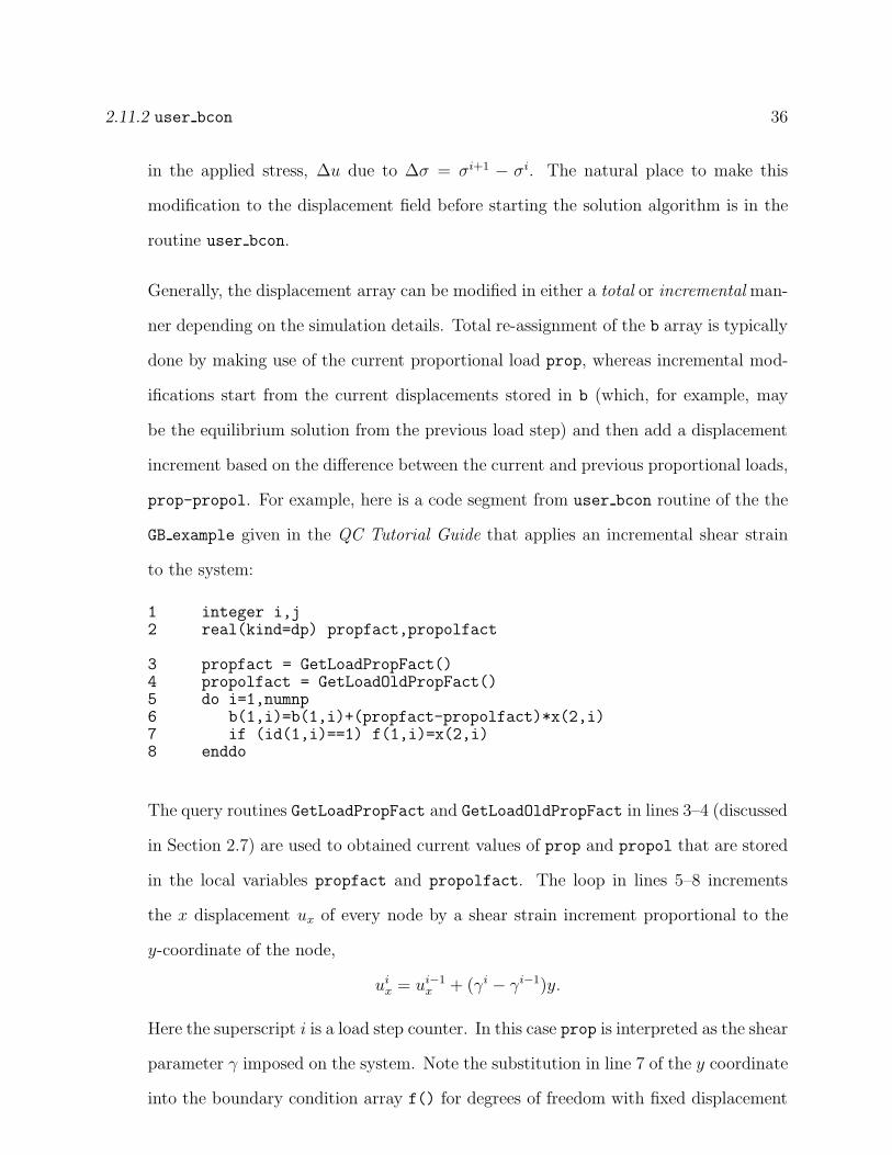
prop-propol. For example, here is a code segment from user bcon routine of the the
GB example given in the QC Tutorial Guide that applies an incremental shear strain
to the system:
1 integer i,j2 real(kind=dp) propfact,propolfact
3 propfact = GetLoadPropFact()4 propolfact = GetLoadOldPropFact()5 do i=1,numnp6 b(1,i)=b(1,i)+(propfact-propolfact)*x(2,i)7 if (id(1,i)==1) f(1,i)=x(2,i)8 enddo
The query routines GetLoadPropFact and GetLoadOldPropFact in lines 3–4 (discussed
in Section 2.7) are used to obtained current values of prop and propol that are stored
in the local variables propfact and propolfact. The loop in lines 5–8 increments
the x displacement ux of every node by a shear strain increment proportional to the
y-coordinate of the node,
uix = ui−1
x + (γi − γi−1)y.
Here the superscript i is a load step counter. In this case prop is interpreted as the shear
parameter γ imposed on the system. Note the substitution in line 7 of the y coordinate
into the boundary condition array f() for degrees of freedom with fixed displacement

2.11.2 user bcon 37
boundary conditions. This is necessary since any modification to displacement degrees
of freedom for which id(i,j)=1 will be overwritten by the next call to compute the
total energy or solve the system (see the discussion of the application of boundary
conditions above).
• dr(ndf,numnp): (double precision) Out-of-balance force vector. Note that this vari-
able should not be modified by the user bcon routine.
• db(ndf,numnp): (double precision) Nodal displacement increment. Note that this
variable should not be modified by the user bcon routine.
• shp(nshp,numel): (double precision) Shape functions. Note that this variable
should not be modified by the user bcon routine.
• xsj(numel): (double precision) Element areas. Note that this variable should
not be modified by the user bcon routine.
• key: (character(len=4)) Key passed from the input file command line. Can be used to
implement various options in user bcon. Note that this variable should not be
modified by the user bcon routine.
• input: (character(len=80)) Input data passed from the input file command line. input
can be used to pass character, double precision, integer or logical data directly from
the command line to the user bcon routine. It is left to the user to parse this data,
however the following is a useful example of how this can be efficiently achieved.
Suppose that the user has written a bcon routine that, in addition to the key option,
requires 3 data entries: a character filename, an integer index and a double precision
scale. The bcon command appears in the input file as:
bcon,key,filename,0,1.0
Everything beyond the second comma will be passed to the user bcon subroutine as
the input variable. Thus, in this example,

2.11.3 user pdel 38
input=‘filename,0,1.0’
The following code segment will effectively parse this input string:
integer lower,upper,next,index,idumreal(kind=dp) scale,dumcharacter(len=80) input,filename...lower = 0upper = next(lower,input)filename = input(lower+1:upper-1)lower = upperupper = next(lower,input)call freein(input,lower,upper,index,dum,1)lower = upperupper = next(lower,input)call freein(input,lower,upper,idum,scale,2)
See Section 2.11.1 for an explanation of the integer function next and subroutine
freein used here.
• flag: (logical) user bcon flag. flag is a global (static) logical variable reserved for the
user bcon subroutine. It can be set as the user likes, for example as an indication of
whether the bcon routine is being called for the first time. It is initialized to .false.
once at the start of the simulation.
2.11.3 user pdel
The routine user pdel is associated with macro pdel (see Section 4.13) that outputs the
current value of prop (see Section 2.7) and a scalar, user-defined, force measure of the
current applied loading. The calling format for pdel is:
pdel,[key],fileprefix[,data]
Macro pdel calls user pdel to computes force. user pdel has the following header:
subroutine user_pdel(id,x,ix,f,jdiag,str,eps,q,b,dr,db,shp,& xsj,key,input,force)use mod_uservarsuse mod_global, only : dp,maxel,maxneq,maxnp,ndf,ndm,nen,nq,nstr,

2.11.3 user pdel 39
& numnp,nxdmimplicit none
!-- Transferred Variablesreal(kind=dp), intent(inout) :: b(ndf,maxnp),str(nstr,maxel),
& eps(nstr,maxel),q(nq,maxel),& x(nxdm,maxnp),f(ndf,maxnp),& dr(ndf,maxnp),db(maxneq),& shp(3,nen,maxel),xsj(maxel)integer, intent(inout) :: jdiag(maxneq),ix(nen,maxel),
& id(ndf,maxnp)character(len=80), intent(in) :: inputcharacter(len=4), intent(in) :: keyreal(kind=dp), intent(out) :: force
The routine uses mod global, which contains dimensioning variables for the transferred
arguments, and dp, the double precision kind variables. These variables are described in
Section 2.1. Note the use of the only clause in the use statement. This is encouraged as a
good programming practice (see Section 2.11.1 for more on this). The variables passed to
user pdel as arguments are defined in Section 2.2, except for the last three that are:
• key: (character(len=4)) The key from the pdel command line.
• input: (character(len=80)) The input string from the pdel command line, including
the fileprefix and [data] exactly as it appears.
• force: (double precision) The scalar measure of the applied force. This is the only
expected output from the routine and is the only external variable that should be
modified by user pdel.
Typically, the force measure can be extracted directly from the values of prop*f(j,i)
for the degrees of freedom to which forces are applied externally, or from dr(j,i) for degrees
of freedom that are constrained to fixed displacements. The units of force in QC are derived
from the energy and length units of the underlying atomistic potentials, typically they are
eV/A.
As an example, here is a code segment from the user pdel routine of the the GB example
given in the QC Tutorial Guide:

2.11.4 user potential 40
integer i
force = 0.0_dpdo i = 1,numnp
if (id(1,i)==1 .and. x(2,i)>0.0_dp) force=force-dr(1,i)enddo
This routine computes the total force in the x direction for nodes with fixed displacements
that have y > 0. In this problem the model is a rectangular region with the bottom at y = 0
held fixed at zero displacement and the top at y = h pulled to the right and held fixed. (See
Section 4.2 and Section 4.2 of the QC Tutorial Guide.) The only nodes with id(1,i)==1
and y > 0 are then the nodes at the top of the model. Therefore the force computed is
the total force that must be applied to the top of the model to hold it at the current shear
strain defined by prop.14 One thing to note is that force is computed as the negative of
dr(). This is due to the sign convention adopted for dr.
2.11.4 user potential
The routine user potential allows the user to define an additional external potential energy,
called user energy that is added to the total energy of the system. This can be used to
include additional boundary conditions that cannot be included using user bcon.
WARNING: If a user energy is defined in user potential, the user must also add the
gradient of this energy to the out-of-balance force vector dr and the second gradient to
the stiffness matrix tang. Otherwise gradient-based solvers (such as conjugate gradients)
or second-gradient based solvers (such as Newton-Raphson) will fail. It is recommended
to perform a numerical derivative checks using the chec macro (see Section 4.3) to verify
that the forces (chec,forc) and stiffness matrix (chec,stif) are computed correctly when
user potential is used.
As an example, consider the repulsive force-field approach used to model cylindrical and
spherical indenters proposed by [15]. The idea is to add to the total energy a potential of
14Without the condition x(2,i)>0.0 dp the force computed would be zero, since the load applied to thetop of the model is balanced by the reaction forces at the support.

2.11.4 user potential 41
the form,
P =N
∑
i=1
ri<R
1
2K(R − ri)2,
where N is the number of nodes in the mesh, R is the radius of the indenter, K is a stiffness
associated with the repulsive field, and ri is the distance between the current position of
node i (xi) and the current position of the center of the indenter (c),
ri = |xi − c|.
The first and second gradients of P follow as
∂P
∂xim
= K(R
ri− 1)(cm − xi
m) (1)
∂2P
∂xim∂xj
n
= δijK
[
R
(ri)3(cm − xi
m)(cn − xin) − δmn
(
R
ri− 1
)]
(2)
In the QC implementation, the variables defining the indenter are stored in module uservars
(see Section 2.11):
module mod_uservarsuse mod_global, only : dp
savepublic
integer user_iparam(10)real(kind=dp) user_rparam(10)
real(kind=dp) indent_radius,indent_radius2,indent_stiffness,& indent_orig(2),indent_force(2)=0.0_dp
end module mod_uservars
Here indent radius=R, indent stiffness=K, and indent orig(2)=c0, where c0 is the
original position of the indenter center at the start of the loading. The other variables
are indent radius2=R2 (stored for computational efficiency) and indent force(2), which
is the force the indenter is applying to the surface (this is returned by user pdel). The
user potential code implementing the repulsive potential is given below:

2.11.4 user potential 42
1 subroutine user_potential(id,x,ix,f,jdiag,str,eps,q,b,dr,shp,xsj,2 & fls,flt,flw)3 use mod_uservars4 use mod_global, only : dp,maxneq,maxnp,maxel,ndf,nen,nq,nstr,5 & numnp,nxdm,user_energy6 use mod_pload, only : GetLoadPropFact,GetLoadOldPropFact,7 & GetLoadTime,GetLoadTimeStep8 use mod_stiff, only : tang,istiff9 implicit none
!-- Transferred Variables10 real(kind=dp), intent(inout) :: b(ndf,maxnp),str(nstr,maxel),11 & eps(nstr,maxel),q(nq,maxel),12 & x(nxdm,maxnp),f(ndf,maxnp),13 & dr(ndf,maxnp),shp(3,nen,maxel),14 & xsj(maxel)15 integer, intent(inout) :: jdiag(maxneq),ix(nen,maxel),16 & id(ndf,maxnp)17 logical, intent(in) :: fls,flt,flw
!-- Local Variables18 integer i,idf,m,n,is19 real(kind=dp) r,r2,del(2),grad_node(2),indent_loc(2),R_over_r,20 & stif_node
21 ! update indenter position22 indent_loc(1) = indent_orig(1)23 indent_loc(2) = indent_orig(2) - GetLoadPropFact()
24 ! compute external potential and forces25 if (flw) user_energy = 0.0_dp26 indent_force = 0.0_dp27 do i=1,numnp28 del(1:2) = x(1:2,i) + b(1:2,i) - indent_loc(1:2)29 r2 = del(1)*del(1) + del(2)*del(2)30 if (r2<=indent_radius2) then31 r = sqrt(r2)32 R_over_r = indent_radius/r33 if (flw) user_energy = user_energy +34 & 0.5_dp*indent_stiffness*(indent_radius-r)**235 grad_node(1:2)= -indent_stiffness*(R_over_r - 1.0_dp)*del(1:2)36 indent_force = indent_force + grad_node37 if (fls) dr(1:2,i) = dr(1:2,i) - grad_node(1:2)38 if (flt) then39 idf = (i-1)*ndf40 do m=1,241 do n=m,242 stif_node = R_over_r/r2*del(m)*del(n)43 if (m == n) stif_node = stif_node - (R_over_r - 1.0_dp)44 is=istiff(idf+m,idf+n,jdiag)45 tang(is) = tang(is) + indent_stiffness*stif_node46 enddo47 enddo58 endif
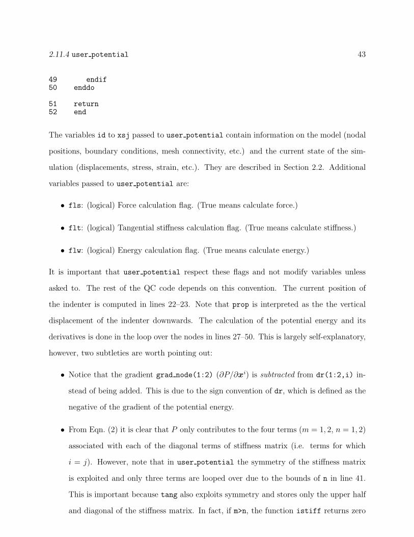
2.11.4 user potential 43
49 endif50 enddo
51 return52 end
The variables id to xsj passed to user potential contain information on the model (nodal
positions, boundary conditions, mesh connectivity, etc.) and the current state of the sim-
ulation (displacements, stress, strain, etc.). They are described in Section 2.2. Additional
variables passed to user potential are:
• fls: (logical) Force calculation flag. (True means calculate force.)
• flt: (logical) Tangential stiffness calculation flag. (True means calculate stiffness.)
• flw: (logical) Energy calculation flag. (True means calculate energy.)
It is important that user potential respect these flags and not modify variables unless
asked to. The rest of the QC code depends on this convention. The current position of
the indenter is computed in lines 22–23. Note that prop is interpreted as the the vertical
displacement of the indenter downwards. The calculation of the potential energy and its
derivatives is done in the loop over the nodes in lines 27–50. This is largely self-explanatory,
however, two subtleties are worth pointing out:
• Notice that the gradient grad node(1:2) (∂P/∂xi) is subtracted from dr(1:2,i) in-
stead of being added. This is due to the sign convention of dr, which is defined as the
negative of the gradient of the potential energy.
• From Eqn. (2) it is clear that P only contributes to the four terms (m = 1, 2, n = 1, 2)
associated with each of the diagonal terms of stiffness matrix (i.e. terms for which
i = j). However, note that in user potential the symmetry of the stiffness matrix
is exploited and only three terms are looped over due to the bounds of n in line 41.
This is important because tang also exploits symmetry and stores only the upper half
and diagonal of the stiffness matrix. In fact, if m>n, the function istiff returns zero

2.11.5 user plot 44
indicating that no such term is stored in tang. For more details on tang and istiff
see Section 2.10.
2.11.5 user plot
The routine user plot provides the user with the opportunity to generate an application-
specific plot. user plot is called whenever a plot,user statement appears in the input file.
The calling format for this statement is
plot,key,filepref,[index],[umag],[scale],[append][,data]
where key=user in this case. The variables filepref and append have their usual meanings
for a plot statement (see Section 4.14 for more information). The file filepref Uxxx.plt
is opened and the file handle pointing to it is passed to user plot. The variables index,
scale and append are also passed to user plot (see below). In addition, variables specific
to user plot may follow the append variable at the end of the input list.
The header of the user plot routine is
subroutine user_plot(id,x,ix,itx,f,jdiag,str,eps,q,b,dr,db,shp,& xsj,index,umag,scale,logic,input,upper)use mod_uservarsuse mod_global, only : dp,maxnp,maxel,maxneq,ndf,nen,nq,nstr,nxdmimplicit none
!-- Transferred Variablesreal(kind=dp), intent(in) :: b(ndf,maxnp),str(nstr,maxel),
& eps(nstr,maxel),q(nq,maxel),& x(nxdm,maxnp),f(ndf,maxnp),& dr(ndf,maxnp),db(maxneq),& shp(3,nen,maxel),xsj(maxel),& umag,scaleinteger, intent(in) :: jdiag(maxneq),ix(nen,maxel),
& id(ndf,maxnp),itx(3,maxel),& index,logicinteger, intent(inout) :: uppercharacter(len=80), intent(in) :: input
The variables id to xsj contain information on the model (nodal positions, boundary condi-
tions, mesh connectivity, etc.) and the current state of the simulation (displacements, stress,
strain, etc.). They are described in Section 2.2. These variables are passed to user plot in
3.0 Head Stage Commands 45
case they are needed for the calculations performed there. They should not be modified.
The variables index, umag and scale are defined in Section 4.14. Note that it is up to the
user to use these variables in user plot in a manner consistent with their definition. (See
subroutine dumpit in module mod plotting for an example how these variables are used.)
Additional plot-specific variables passed to user plot are:
• logic: (integer) File handle to an open plot file. Data is sent to this file using standard
Fortran output statements:
write(logic,format-spec) list
where format-spec is the format specifier (use * for unformatted output), and list is
the list of data variables to be written.
• input: (character(len=80)) The input line containing all of the variables and delimiters
after the key parameter (i.e. input = ‘filepref,index,umag,scale,append,data’).
The user may parse this string to obtain additional variables in data specific to
user plot. See the discussion for the upper variable appearing next.
• upper: (integer) A pointer to the last comma or end-of-line symbol that was processed
in the input line. (This is the comma between append and data.) The user may
continue parsing the string from this point as shown in Sections 2.11.1 and 2.11.2.
3 Head Stage Commands
The following is an alphabetical listing of the commands that are available during the head
stage of the QC simulation. For additional detail, please see the QC Tutorial Guide.
3.1 Macro ’cons’ : read in potential specific constitutive input
The default module for the cons routine is a module that reads a general EAM [6] potential
from a file in either setfl or funcfl format. These formats are standard with the MD

3.1 Macro ’cons’ : read in potential specific constitutive input 46
code DYNAMO [16]. Potentials from other sources can be converted to the setfl format
using the utility program dynpots.f provided with the QC code. The dynpots.f file can
be found in the QC subdirectory Potentials/FortranSource. The QC method expects all
interatomic potential files to have the .fcn extension.
Funcfl files contain only the potential information for a single atom type, while all
pair-potential interactions between dissimilar nuclei are modeled as the geometric mean of
the homonuclear pair interactions. Setfl files contain all the potential information for a
complete alloy set, including the pair-potential interactions between the dissimilar nuclei.
They can also be used for potentials defining a single atomic species.
calling format: cons,key,nfiles,fprefix 1,...,fprefix nfiles
• key:
– ’setf’ : File containing constitutive information is in setfl format.
– ’func’ : Files containing constitutive information are in funcfl format.
• nfiles : (integer) The number of files required to read all the necessary constitutive
information. Note that if the key is ’setf’, this value must be 1.
• fprefix i : (character(len=80)) The file prefix for the name of a file, fprefix i.fcn,
containing the constitutive information. The number of file prefixes must equal nfiles.
After all the constitutive information has been read in, the cons command computes
several values for each of the previously defined grains in the model. Specifically, it computes
the cohesive energy per unit volume, the initial stresses and the initial elastic moduli for the
infinite, undistorted lattice. The stresses and moduli are given in relation to the global x-
y-z coordinate system, and the moduli are presented in the compact Voigt notation using
a 6 × 6 matrix. These values are often known from atomistic simulations of the same
material and serve as a useful check that the grains and constitutive information have been
read in correctly. The user can access the elastic constants (perhaps in order to apply

3.2 Macro ’end ’ : terminate head stage 47
boundary conditions in user bcon) using the routine GetGrainRefStiff in mod grain (see
Section 2.4). The initial stresses in the perfect lattice should be zero. Often, very small
differences between the lattice constant used to define the grains and the optimal lattice
constant can lead to nonzero residual stresses in the lattice.
3.2 Macro ’end ’ : terminate head stage
calling format: end
This command is required to signal the end of the head stage.
3.3 Macro ’fact’ : sets global run factors
There are a number of factors that need to be set by the user at the start of a QC simulation.
This is achieved using the fact command. In a typical input file, a list of these commands
will appear near the start of the file. Factors can be set in any order. Even if the default value
is to be used, it is often useful (for clarity) to include these commands in the simulation.
calling format: fact,key,value
• key :
– ’prox’ : Proximal nonlocality factor (PROXFACT). See Section 4.21 for more de-
tails.
– ’adap’ : Adaption nonlocal padding factor (ADAPFACT). See Section 4.1 for more
details.
– ’cutf’ : Effective cutoff factor (CUTFACT). See Section 4.21 for more details
– ’epsc’ : Nonlocality criterion strain tolerance (epscr). See Section 4.21 and
Section 3.2 of the QC Tutorial Guide for more details.
• value : (double precision) The factor will be set to this value.
Note: For more information on the run factors, see the file mod global.f.

3.4 Macro ’flag’ : sets global run flags 48
3.4 Macro ’flag’ : sets global run flags
The flag command is exactly like the fact command, except that it is reserved for simulation
parameters that are of logical type. These are typically switches that determine whether or
not a particular feature of the QC will be activated for the current simulation.
In a typical input file, a list of flag commands will appear near the start of the file.
Flags can be set in any order. Even if the default value is to be used, it is often useful for
clarity to include these commands in the simulation.
calling format: flag,key,value
• key :
– ’nloc’ : Nonlocal effects flag. (Default, NlocOn=T)
– ’surf’ : Surface effects flag. See Section 2.11.1 for more details. (Default,
SurfOn=T)
– ’grai’ : Grain boundary effects flag. See Section 3.5 for more details. (Default,
GrainOn=T)
– ’ghos’ : Ghost force correction flag. (Default, GhostOn=T)
– ’node’ : Nodes on Bravais sites flag. Note that this flag must be set to T if
nonlocal effects on being included in the simulation. (Default, NodesOnBsites=T)
– ’prev’ : Element warping prevention flag. (Default, PreventWarping=F) Ele-
ment warping occurs when the deformation is so severe that the volume of an
element becomes zero or negative (the element is turned “inside-out”). This is
not permitted in continuum finite elements and in QC elements touching local
repatoms. However, elements between nonlocal repatoms contain no atoms and
can warp without any non-physical consequences. Typically then, PreventWarping
is set to false. In a fully local simulation, setting this flag to true can be a useful
check for errors in the model.

3.4 Macro ’flag’ : sets global run flags 49
– ’defm’ : Perform mesh adaptions in the deformed configuration. (Default,
DefMesh=F)
– ’dumm’ : Flag indicating that “dummy atoms” are permitted. Dummy atoms are
atoms stored inside local elements near that local/nonlocal interface. They are
required to ensure the nonlocal repatoms see all their neighbors unless the local
elements are fully refined in this region. Usually, allowing dummy atoms permits
more rapid coarsening of the local elements but they will lead to larger ghost
forces at the interface. If this flag is set to false, it forces the adaption routine to
fully refine the local region immediately surrounding any nonlocal region, out to
one cutoff radius of the potentials.
NOTE: If this flag is set to false it may result in premature termination of conju-
gate gradient minimization. The reason for this is that during conjugate gradient
minimization dummy atoms may move into the cutoff radius of nonlocal atoms.
This is detected by periodic neighbor list updates that are carried out. If this
occurs the conjugate gradient routine will exit with a warning. To ensure that
minimization is completed with the DummysAllowed flag set to false, the conju-
gate gradient solver call needs to be placed inside a loop:
loop,,5solve,cg,1.0,10000,1status,updateconvergence,force
next
No change is required for Newton-Raphson minimizations.(Default, DummysAllowed=T).
• value : logical, true sets the flag to true, turning on the effect it controls. False turns
the effect off.
Note: For more information on the run flags, see the file mod global.f.

3.5 Macro ’grai’ : read in grain structure information, initialize grains 50
3.5 Macro ’grai’ : read in grain structure information, initializegrains
calling format: grai,key[,fileprefix]
• key:
– ’file’ : Read the grain structure data from a file called fileprefix.geo.
– ’dire’ : Read the grain structure data from the input stream in the lines following
the grai command.
• fileprefix: (character(len=80)) Name of the file to be read if key=’file’. Note
that the program appends the extension .geo to form the filename.
Note: For information on grain structure data format, see Section 3.5 of the QC Tutorial
Guide and subroutine ReadGrainData in the file QC/Code/mod grain.f.
3.6 Macro ’mate’ : material data input
calling format: mate,key[,nfiles,fprefix1,fprefix2,...]
• key :
– ’file’ : Read the material data from a files whose names appear in the command
line, (fprefix1,fprefix2,...).
– ’dire’ : Read the material data from the input stream in the lines following the
mate command.
• nfiles : (integer) The number of files to be read to obtain all the material definitions
if key=’file’.
• fprefix : (character(len=80)) The prefix of the name of the file to be read if key=’file’.
There must be nfiles names in the list. Note that the program automatically appends
the extension .mat to create the filename.
3.7 Macro ’mesh’ : generate mesh 51
Note: For more detail, see the discussion of this command in Section 3.3 of the QC
Tutorial Guide.
3.7 Macro ’mesh’ : generate mesh (user mesh routine)
calling format: mesh[,key][,data]
This routine calls a user-supplied routine user mesh to generate the initial mesh. See Sec-
tion 2.11.1 for a detailed description of this routine. The optional parameters key and data
are passed to user mesh. By convention key=’dire’ implies that any data to user mesh is
given in the lines following the mesh statement, otherwise the data is expected to be in the
remainder of the statement that is stored in data. It is up to user mesh to conform to these
conventions. Upon return from this routine an initial mesh will have been defined including
the coordinates of all nodes and the mesh connectivity.
WARNING: QC does not perform any validation checks on the results of the user mesh
routine. If this routine is faulty it could results in erratic behavior of the code.
3.8 Macro ’zone’ : define special-attribute zones
calling format: zone,key,[fprefix][,index]
Special-attribute zones are regions in the model where a user can introduce special constraints
on the nodes. Currently, two possibilities exist. No-adaption zones are regions where no
adaption is allowed and all nodes are required to be local. These zones are typically placed
to cap nonlocal regions that would otherwise continue to extend throughout the model further
than desirable. An example of this is shown in Section 3.4 of the QC Tutorial Guide for
a grain boundary. Nonlocal zones are regions where all atoms must be nonlocal. This is a
convenient way for introducing a nonlocal region where it otherwise would not be triggered.
• key :
– ’file’ : Read special-attribute zone data from a file named fprefix.zon.

4.0 Macros Stage Commands 52
– ’dire’ : Read special-attribute zone data from the input stream in the lines
following the zone command.
• fprefix : (character(len=80)) Prefix of the file to be read if key=’file’. Note that
the program automatically appends the extension .zon to create the filename.
• index:
– 0,1 : No-adaption zone. All nodes in this region must be local. No adaption is
allowed in this region.
– 2 : Nonlocal zone. All nodes in this region must be nonlocal. If there is at least
one node in the zone, it will result in the entire region being refined down to the
atomic scale and made nonlocal.
Note: For information on the special-attribute zone data format, see Section 3.4 of the QC
Tutorial Guide and subroutine ReadZone in file Code/mod boundary.f.
4 Macros Stage Commands
The following is an alphabetical listing of the commands that are available during the macros
stage of the QC simulation. For additional detail, please see the QC Tutorial Guide.
4.1 Macro ’adap’ : Automatically adapt the mesh, through meshrefining and coarsening
The adap command is the starting point for all mesh adaption, including both mesh refine-
ment and mesh coarsening. Related commands include prot and the mesh command in the
head stage of the simulation. The adaption uses an estimator for the error in the deformation
gradients, based on the error estimator of Zienkiewicz and Zhu [17] and described in more
detail in [3].
Note that the last action of the adap command is a forced call to the status command
to re-compute the repatom statuses. If necessary, this will trigger iterative adaption to make

4.2 Macro ’bcon’ : apply boundary conditions 53
sure all nonlocal repatoms represent only themselves. See Section 4.21 for more details.
calling format: adap,,vartol,icoarse
• vartol : (double precision, default=0.075) Adaption criterion trigger value. Any
element with a refinement criterion value greater than vartol will be refined. If coars-
ening is active, then any element that can be removed without creating new elements
which would satisfy the refinement criterion is removed.
• icoarse : (integer, default=0) Specifies whether coarsening is active.
– icoarse=0: indicates coarsening is off.
– icoarse=1: indicates coarsening is on.
4.2 Macro ’bcon’ : apply boundary conditions (user bcon routine)
calling format: bcon[,key][,data]
The bcon command calls a user-supplied subroutine called user bcon, and permits the user
to define key options and input data as required. As a result, the input for the command
will depend on the user routine. The details of the functions performed by the bcon routine
are also largely dependent on the user’s requirements. For a detailed description of this
routine see Section 2.11.2.
4.3 Macro ’chec’ : Numerical derivative check
chec computes the first and second derivatives of the total energy numerically and compares
them to the analytically computed values. It is for debugging purposes only, and is helpful
when implementing new potentials or other changes to the code.
Note that some small discrepancies in the stiffness elements will often occur with inter-
atomic potentials in the tabulated form provided with the QC package. This is due to the
interpolation of higher order derivatives of the tabulated potentials. These discrepancies
have not been found to interfere substantially with solution convergence.
calling format: chec[,key][,code]

4.3 Macro ’chec’ : Numerical derivative check 54
• key:
– ’ ’ or ’forc’ : Numerical derivative check of out-of-balance forces. Compares
analytical derivative with numerical derivative. Results are sent to the log file and
the Tecplot R© file forcecheck.plt.
Note: macro form must be called before this to set up the out-of-balance
force vector.
– ’stif’ : Numerical derivative check of stiffness matrix. Results are sent to the
log file. Any stiffness matrix components which fail the test are flagged with a
<---*** marker. Parameter code sets the number of repatoms tested:
∗ code=0 : Check is carried out for two arbitrary rep atoms, one local and
one nonlocal, i.e. all stiffness matrix items associated with these atoms are
tested. This option should be selected for large meshes where testing the
entire stiffness matrix would be computationally prohibitive. This is the
default.
∗ code=1 : One local atom and all nonlocal atoms are tested. Use this for
medium sized models.
∗ code=2 : All atoms are tested. Use this for small models.
Note: macro tang must be called before this to set up the stiffness matrix.
– ’loca’ : Numerical derivative check of the stresses and moduli computed in the
potential routine for the local limit. Parameter code sets the deformation gradient
for which the test will be done:
∗ code = 0 : The check is done using a randomly selected deformation gradient
hard-wired into the routine. This is the default.
∗ code = iel : The check is done using the deformation gradient of element
iel.

4.4 Macro ’clea’ : Re-initialize solution variables. 55
Note: regardless of the deformation gradient selected by code the test will be
carried out for all grains in model. This means that if code=iel is selected and
there are more than one grains in the model, the deformation of element iel will
also be used to test grains with which that element is not associated.
• code: (integer) See the key-dependent descriptions above.
4.4 Macro ’clea’ : Re-initialize solution variables.
calling format: clea
clea sets the nodal displacement vector b and the last increment in the nodal displacements
db to zero.
4.5 Macro ’conv’ : Loop convergence test
The conv command is used within a loop . . . next construct to test for convergence. If
convergence has been achieved, the loop is terminated and the simulation proceeds from the
first command following the next command of the terminated loop.
The conv command can also be used to force a load step to exit. At the start of each
call to the conv routine, the program looks for a file abort.dat in the working directory of
the simulation. If the first line of this file contains a single T (for .true.) a “converged”
signal is returned from the conv command regardless of the current convergence measure.
In this way, the user can stop a simulation but still produce, for example, output of the last
incomplete load step.
A related command is tole, which sets the value of globaltol used by the conv routine.
calling format: conv,[key]
• key :
– ’ ’ or ’forc’ : converge when out-of-balance force norm is reduced below
globaltol*rnmax where rnmax is the largest force norm encountered in the cur-
rent loop.

4.6 Macro ’dtim’ : set time increment 56
– ’disp’ : converge when the norm of the last displacement increment taken in the
solver is less than globaltol.
– ’cdis’ : converge when the norm of the last displacement increment taken in the
solver is less than a fraction (globaltol) of the maximum displacement increment
norm encountered in the loop.
– ’ener’ : converge when the change in energy in the last Newton-Raphson step
is less than globaltol.
– ’elem’ : converge when the current number of elements is the same as or less
than the number of elements the mesh had the last time conv was called. Used
as a check to see when mesh refinement is no longer occurring.
– ’adel’ : same as ’elem’, but current number of elements is compared to the
number of elements that existed prior to the last mesh adaption.
– ’pdel’ : converge when the difference between the current external load (com-
puted by macro ’pdel’) and the external load when conv was last called, is less
than globaltol.
– ’nnln’ : converge when the number of nonlocal nodes (i.e. repatoms) is the same
or less than it was the last time this convergence test was called. The value of
globaltol should be set to a number less than 1.0.
4.6 Macro ’dtim’ : set time increment
calling format: dtim,,dt
Note that there is no key required for this command, and so the double-comma is required
to denote an empty key field.
• dt: (double precision). Time increment to be used by the time command .
4.7 Macro ’form’ : Form the out-of-balance force vector
calling format: form

4.8 Macro ’ghos’ : Compute ghost forces correction 57
The form command computes the out-of-balance forces and total energy for the current
nodal displacements.
4.8 Macro ’ghos’ : Compute ghost forces correction
calling format: ghos
The ghos command computes the ghost force corrections associated with the current mesh,
repatoms statuses and displacements. In all subsequent computations of the out-of-balance
forces, the ghost force corrections will be added as dead loads to minimize the spurious
forces at interfaces between local and nonlocal regions. If the status or adap command
is called after the ghos command, it will generally change the values of the ghost forces.
For this reason, the execution of the status or adapt commands will automatically force a
re-computation of the ghost force correction loads.
The ghost force correction is described in detail in [3]. Note that the magnitudes and
directions of the spurious forces will change as the repatom displacements change, and thus
the ghost forces should in principal be updated occasionally during the simulation. It is left
to the user to determine when these ghost forces need to be updated.
Since the ghost force correction is an approximate fix, there is necessarily some level of
error associated with a QC simulation, even with ghost forces corrected using this command.
The main source of this error lies in the fact that the ghost force correction is only periodically
updated (at all status calls and explicit calls to this ghost command) and added as dead
loads. In fact, every change to the displacement fields during the solution algorithm will
change the ghost forces slightly, but the lack of a well-defined energy functional incorporating
the ghost forces makes their complete elimination impractical.
In order for the ghos command to have an effect, the GhostOn flag must be set to .true.
during the head stage of the simulation.

4.9 Macro ’loop’ : set loop start indicators 58
4.9 Macro ’loop’ : set loop start indicators
The loop command indicates the start of a loop in the command structure. The current QC
implementation permits full loop nesting to any depth.
calling format: loop,[label],nloop
• label : (character) label name for the loop (only used as a guide to the eye - program
does not verify loop-next labels match).
• nloop: (integer) number of times the loop is to be executed unless prematurely termi-
nated due to a “converged” signal from the conv command.
4.10 Macro ’mark’ : set or return to a marked state of the sim-ulation
The mark command is used to mark a stage in the simulation (essentially a displacement
field and mesh) or to return to a previously marked state.
calling format: mark[,key]
Where there are two options for key:
• key=’set’ : set the mark and store the current mesh configuration and displacements.
• key=’go’ : restore the displacements to those at the previous mark. If adaption
has taken place since the mark was set, new nodes are given their displacements by
interpolation.
An example of using mark is in the simulation of dislocation nucleation. It is desirable is
such simulations to iteratively adapt the pre-nucleated state so that the dislocation will not
be artificially influenced by the mesh. As such, mark can be used in conjunction with the
conv,nnln convergence option to restart from the displacement field prior to the nucleation
event. The following input file segment illustrates the idea (relevant commands highlighted
by the comments):

4.11 Macro ’next’ : loop terminator control 59
loop,load,40
bcon
mark,set % here is where the mark is set
loop,,10
mark,go % here is the return to a previous mark
solve,cg,1.0,500000,1
status
conv,nnln % if the number of nonlocal nodes
% changes, this forces a return to the
% previous mark
next
solve,cg,1.0,500000,1
plot,disp,gbshear,0,1.,1.
report
pdel,,p-delta
restart,write,shear
time
next,load
4.11 Macro ’next’ : loop terminator control
The next command indicates the end of a loop (started by a loop command) in the command
structure.
calling format: next[,label]
Description of input variables:
• label : (character(len=4)) label name for the loop (only used as a guide to the eye -
program does not verify that loop-next labels match).

4.12 Macro ’outp’ : output nodal displacements to the log file 60
4.12 Macro ’outp’ : output nodal displacements to the log file
calling format: outp
The command outp writes the nodal displacements to the log file.
4.13 Macro ’pdel’ : compute current external load and applieddisplacement
calling format: pdel,[key],fileprefix[,data]
The pdel command is used to produce output of a scalar measure of the applied force
for a given configuration.15 It opens a file fileprefix.pde at its first call and at this
and subsequent calls writes a line of output to the file. The output line consists of two
real numbers: the current value of prop (the proportional load level) and a user-defined
measure of the applied force. The force is computed by the routine user pdel, which must
be supplied by the user and is documented in Section 2.11.3. More information on prop is
given in Section 4.15. The arguments to the pdel command are:
• key : (character(len=4)) Optional parameter passed to the user routine user pdel.
This could be used, for example, to select a particular force when the routine has
multiple options.
• fileprefix : (character(len=80), default = ’pdelta’) Prefix of file to which the output
should be written. The program will automatically append the extension .pde to
create the filename fileprefix.pde.
• data : Optional data passed to the user routine user pdel. This can include a list of
variables separated by commas that will be parsed by user pdel. See Section 2.11.3
for more information.
15The name “pdel” comes from the original use of this feature for plotting the load (P ) versus depth (δ)in nanoindentation simulations.

4.14 Macro ’plot’ : write out plot file in Tecplot R© format 61
4.14 Macro ’plot’ : write out plot file in Tecplot R© format
calling format: plot,key,filepref,[index],[umag | polyfile],[scale],[append]
• key :
– ’ ’ or ’disp’ : Displacement field plot. The nodal x, y and z displacements
are stored on a finite element mesh plot. For this key, index has no effect.
– ’bcon’ : Boundary conditions plot. Finite element mesh plot with the following
nodal values:
∗ index = 0,1 : applied loads.
∗ index = 2 : out-of-balance forces.
∗ index = 3 : boundary condition indicator (0 free, 1 constrained).
– ’stre’ : Kirchhoff stress field plot. Finite element mesh plot with the following
nodal values:
∗ index = 0 : Von Mises effective stress.
∗ index = 1 : Kirchhoff stress components: σxx, σyy, σzz, σxy, σxz, σyz .
Notes:
1. Stresses are element quantities that are computed at the element integration
points. The nodal values stored in the plot file are extrapolated and thus
include an additional extrapolation error.
2. Stresses are only computed in elements adjacent to local nodes. No stress
information is available in nonlocal regions.
3. The output stresses are components of the Kirchhoff stress tensor τ not the
more commonly used Cauchy stress tensor σ. See variable str in Section 2.2
for the relation between these stress measures.
– ’stra’ : Lagrangian strain field plot. Finite element mesh plot with the following
nodal values:

4.14 Macro ’plot’ : write out plot file in Tecplot R© format 62
∗ index = 0 : Von Mises effective strain.
∗ index = 1 : Lagrangian Strain components: ǫxx, ǫyy, ǫzz, ǫxy, ǫxz, ǫyz.
Notes 1 and 2 for key=’stre’ apply here as well.
– ’ener’: Strain energy density field plot. Nodal values of the strain energy density
are extrapolated from the element integration points. For this key, index has no
effect. Notes for key=’stre’ apply here as well. To plot the energies of individual
nonlocal atoms, the ’repa’ key described below should be used.
– ’ghos’: Ghost force correction plot. The nodal ghost force correction dead loads
are plotted on a finite element mesh. index has no effect.
– ’patc’: Patch plot of the internal element variables. This option allows the
user to view the element variables without the extrapolation errors discussed in
key=’stre’. The generated mesh is patched with each element displaying a
constant value. The displayed information is set by index:
∗ index = 0 : Mixed plot with generally useful values:
· Strain energy density.
· Eigenvalues of the right Cauchy-Green deformation tensor C = FTF
(where F is the deformation gradient): λ1 , λ2, λ3.
· σxy (XY -component of the Kirchhoff stress tensor).
∗ index = 1 : Strain Energy Density plot.
∗ index = 2 : Eigenvalues of the deformation tensor FTF , (where F is the
deformation gradient). These values are used in the nonlocality criterion and
indicate the degree of deformation in an element.
∗ index = 3 : Kirchhoff stress plot. Plotted values are: σxx, σyy , σzz, σxy, σxz,
σyz.
∗ index = 4 : Lagrangian strain plot. Plotted values are: ǫxx, ǫyy, ǫzz, ǫxy, ǫxz,
ǫyz.

4.14 Macro ’plot’ : write out plot file in Tecplot R© format 63
– ’repa’: Representative atom plot. Output the nonlocal representative atoms fol-
lowed by the local representative atoms. For each atom its energy and the number
of atoms it represents is included. Following the representative atom information,
the tessellation for the current representation and the model boundaries are added.
For this key, index has no effect.
– ’atom’: Atomic positions plot. Generates a plot of all atoms in a given polygon.
The polygon vertex coordinates are read from file ’polyfile’. The positions of
unrepresented atoms are obtained through finite element mesh interpolation. The
type of plot generated is determined by index:
∗ index = 1 : normal plot
∗ index = 2 : ”Vitek” plot - In addition to the atomic position, adds infor-
mation on the relative slip between the atoms. This is inspired by Prof. V.
Vitek’s visualizations of screw dislocation cores (See, for example, [18]).
– ’type’: Atomic types plot. Plots the atomic number for each repatom, useful
for models where there are more than one species of atom present. For this key,
index has no effect.
– ’user’: User-specified output generated by the routine user plot. The param-
eters index, umag and scale are read in and passed to user plot. The append
setting is respected. Additional user-specified input can be read in after append
if desired. More information on user plot is available in Section 2.11.5.
• filepref : (character(len=80), default = ’qcplot’) The prefix which will be used to
produce the name of the output file. The plot command builds a unique filename for
each plot produced using four components: the user-defined filepref, a letter code
identifying the file type, a unique, automatically incremented 3-digit number and the
.plt file extension. The key-specific letter codes are:
– ’ D’: Displacement (disp) plot.
4.14 Macro ’plot’ : write out plot file in Tecplot R© format 64
– ’ B’: Boundary Condition (bcon) plot.
– ’ e’: Strain (stra) plot.
– ’ s’: Stress (stre) plot.
– ’ E’: Energy (ener) plot.
– ’ G’: Ghost Force (ghos) plot.
– ’ P’: Patched (patc) plot.
– ’ R’: Repatom (repa) plot.
– ’ A’: Atoms (atom) plot.
– ’ t’: Atom Types (type) plot.
– ’ U’: User-specified (user) plot.
For example, if filepref=qcplot, and the key=disp, the filenames generated would
be qcplot D001.plt, qcplot D002.plt, qcplot D003.plt etc. each time a disp plot
is generated.
• index : (integer, default=0) A switch modifying the behavior of each of the key
options. The effects of index for each key are detailed above.
• umag : (double precision, default=0.0) used with key=’disp’, ’bcon’, ’stre’, ’stra’,
’ener’, ’ghos’, ’patc’ and ’user’. Sets the magnification factor for the displace-
ments added to the nodal reference positions. If umag=0.0, plot will be in the reference
configuration. If umag=1.0, plot will be in the deformed configuration. Other values
of umag will appropriately exaggerate or reduce the current displacement field.
• polyfile : (character(len=80), default=’poly.dat’) Only used by key=’atom’. File-
name of the file with the coordinates of the polygon vertices defining the region where
atoms should be plotted.

4.15 Macro ’prop’ : define proportional load table 65
• scale : (double precision, default=1.0) Used with key=’disp’, ’bcon’, ’stre’,
’stra’, ’ener’, ’ghos’ and ’user’. Sets the magnification factor for the output
variable.
• append : (integer, default=0) If append is set to 1, the code will attempt to append
the output as a new Tecplot R© “zone” in an existing file of the same name, rather
than writing each output to a new file. In append mode, the code searches the home
directory for the most recently written file with the same filepref and 2-character
letter code as discussed above, and appends to that file. If no comparable file has been
previously written, a new file is created.
The append option is available for all plot types. Note that in order for it to be
correctly read, all previous data for the command must be present, even if the default
values are to be used or the data is not relevant to that plot type. Said another way,
the code expects append to be the fifth datum after the key on the command line.
So, for example, setting append mode for a repatom plot type requires the command
plot,repa,filepref, , , ,1
to be used.
Because append is the last datum and it is defaulted to 0, it can be omitted if the
append option is not desired.
4.15 Macro ’prop’ : define proportional load table
Loading is incremented in the QC method by variable referred to as the time, despite the
static nature of QC simulations. This time variable is further used to compute a proportional
load variable prop. The prop command is used to define the dependence of the prop variable
on the time variable. This dependence is read in as a set of ordered pairs, between which
QC will linearly interpolate to obtain a piecewise linear function of prop vs time. The prop
versus time curve may contain step functions (i.e. two prop values that have the same time
value). See Section 2.11.2 for an explanation how prop is used in the application of boundary

4.16 Macro ’prot’ : protect existing nodes from being deleted by coarsening 66
conditions.
calling format: prop,,npld,[fileprefix],[time(1),pload(1),time(2),pload(2),. . .]
Description of input variables:
• npld : (integer) Number of points in proportionality graph.
• fileprefix : (character(len=80)) Prefix of file containing graph data. The program
will try to open a file called fileprefix.prp from which to read the data. If the
fileprefix is absent, graph data is read from argument list.
• time(i) : (double precision) time coordinates of a set of points on a piecewise linear
time-proportionality graph.
• pload(i) : (double precision) prop coordinates of a set of points on a piecewise linear
time-proportionality graph.
Note that there is no key required for this command, and so the double-comma is required
to denote an empty key field. Note also that if the values are to be read from the argument
list rather than from a file, a second double-comma must explicitly appear to ensure that
fileprefix is interpreted as an empty string.
4.16 Macro ’prot’ : protect existing nodes from being deleted
by coarsening
If the user plans to take advantage of the mesh coarsening features in the adaptive meshing
algorithm, it is usually necessary to define a set of “protected” nodes that will not be removed
by coarsening and hence prevent the essential features of the mesh geometry from being lost.
The prot command provides a simple means to this end by allowing the user to protect
either all existing nodes or all existing boundary nodes in the current mesh.
calling format: prot[,key]
• key :

4.17 Macro ’repo’ : print out current energy and out-of-balance forces 67
– ’ ’ : protect all nodes in the model.
– ’boun’ : protect all nodes on the model boundaries.
4.17 Macro ’repo’ : print out current energy and out-of-balance
forces
calling format: repo
This command prints a brief report to the output stream including the current value of the
energy and out-of-balance force norm. The latter quantity is of particular interest since it
should be zero (to within some tolerance) for a converged solution.
4.18 Macro ’rest’ : read/write restart files
calling format: rest,key,fileprefix
• key :
– ’read’ : read stored simulation from a previously written binary restart file.
– ’writ’ or ’ ’ : write simulation data to binary restart file.
– ’txrd’ : read stored simulation from a previously written ASCII text restart file.
– ’txwt’ or ’ ’ : write simulation data to ASCII text restart file.
• fileprefix : (character(len=80), default=’qc’) Prefix of the restart file name. The
program will automatically append the .res extension to create the filename for binary
restart files or the .trs extension for ASCII text restart files.
Restart files can be used to prevent loss of simulation results in the event that a QC
simulation is terminated unexpectedly, for example due to a power failure. Restart files can
also be used to re-start a run with different simulation parameters. ASCII text and binary
restart files perform the identical function, but text restarts are typically about 3 times as
large as their binary equivalent. The text version should only be used if portability of the
restart file across different platforms is not possible with the binary format.

4.18 Macro ’rest’ : read/write restart files 68
Each time a restart command is used to write a restart file, the code checks for the
existence of a file fileprefix.res (or fileprefix.trs, as appropriate) in the working
directory. If such a file exists, it is moved to a file fileprefix LAST.res before the new
file is written. In this way, there are up to two restart files saved at a time. Upon a third
attempt to write a restart file with the same name, the same procedure is followed and the
old copy of fileprefix LAST.res is lost.
The only important data not stored in the restart file is the stiffness matrix in order to
avoid unnecessarily large files. The stiffness matrix can easily be recomputed after reading
a restart file using the tang command.
A restart file can be read at any point in the macros stage of the simulation, but are
typically read in as the first macros command. Re-starting from a previously written restart
file is best done by using a new input file with a very similar list of commands in the head
stage. Some changes to the commands in the head are possible, others must be used with
caution, and others will not lead to a successful restart.
Some examples of changes to the head stage that are permissible:
1. Changes to some of the fact settings or flag settings.
2. Changes to the constitutive information (using a different interatomic potential), pro-
vided that the lattice parameter of the new potential is identical to that of the original
one.
3. Changes or additions to the no-adaption zones.
4. Increasing the allocated storage for repatoms (maxnp) or elements (maxel), see Section 3
of the QC Tutorial Guide for more details.
Some examples of changes that must be used with caution:
1. Any changes to the mesh generator will be completely ineffectual, as the rest command
will read in the entire mesh from the restart file and overwrite the generated mesh.

4.19 Macro ’setp’ : store current resultant for comparison in conv,pdel 69
2. Changes to the active/inactive status of any grain boundary segments must be accom-
panied by the appropriate adaptive remeshing after the restart file is read in, since the
newly activated grain boundary may be in a region of coarse mesh and cause nonlocal
atoms to represent large volumes of the material. This will lead to an energy functional
that is a very poor approximation to the correct one.
Some examples of changes that will not lead to a successful restart:
1. Changes to the grain definitions. Modifying the orientation or shape of the grains
will generally not lead to a successful restart. Repatoms in the restart file data will no
longer fall on Bravais lattice sites, as required by the simulation, or elements may fall
entirely outside of the newly shaped grains.
2. Changes to the material definitions. Modifying the Bravais lattice will have a similar
effect to that of modifying the grain orientations.
4.19 Macro ’setp’ : store current resultant for comparison inconv,pdel
calling format: setp
The command setp computes and stores the current value of the user-defined applied force
(using the same user pdel routine described in Section 2.11.3. Each subsequent call to
conv,pdel will compare the current value of the force to that stored at the last call to setp
to decide if convergence has been achieved.
4.20 Macro ’solv’ : call solver routine
The two solvers available in the QC method are a Newton-Raphson (NR) method and
the Conjugate Gradient (CG) method. Both are called from the same command by using
different key options.
calling format: solv,key,dsmax,maxfn,iprint
Description of input variables:

4.21 Macro ’stat’ : Recompute local/nonlocal representative atom status 70
• key :
– ’nr ’ : Newton-Raphson solver
– ’cg ’ : Conjugate Gradient solver
• dsmax : (double precision, default=1.5) Maximum allowed change in a dof in a single
step, units of length.
• maxfn : (integer, default=10000), limit on simulation.
– maxfn>0 : maximum allowed evaluations of the energy and out-of-balance forces
is maxfn.
– maxfn<0 : maximum number of CG iterations is |maxfn|.
• iprint : (integer, default = 0) The number of interactions between CG outputs. E.g.,
if iprint=3 output is written every third CG iteration. If iprint=0, no output is
generated.
Note that parameters maxfn and iprint are only used in the CG routine, but they must
be specified for both solver options. This is because the NR routine includes a error trap
that will attempt to use the CG solver in the event of a NR failure.
4.21 Macro ’stat’ : Recompute local/nonlocal representative
atom status
The stat command should be called whenever there is need to check that current repatom
nonlocal/local status is consistent with the nonlocality criterion. However, it can be a slow
process and must be used judiciously to avoid excessive computational time.
A repatom can be given nonlocal status for one of two reasons. First, if it is within
PROXFACT*rcut of any active surface or grain boundary, it will be made nonlocal. Secondly,
it will be made nonlocal if it is in a region of the crystal that is experiencing significant

4.21 Macro ’stat’ : Recompute local/nonlocal representative atom status 71
variation in the deformation gradient on the atomic scale. Details of this criterion can be
found in [3, 19], and is discussed in more detail in Section 3.2 of the QC Tutorial Guide.
The status command also serves to check that the neighbor lists for the current set of
nonlocal repatoms is up-to-date. This is invoked using stat,update as described below. In
this case, the status is only re-calculated if it is deemed that the deformation since the last
neighbor-list computation is such that neighbor lists may have changed.
calling format: stat[,key]
• key :
– ’ ’ : compute status of all representative atoms in the model and set up
auxiliary arrays, such as neighbor lists, to speed execution.
– ’upda’ : check whether stored auxiliary arrays are up-to-date, and whether the
displacements since the last status calculation are too large, making it necessary
to recompute the lists. Note that this key option does not technically check
whether the status, per se, needs to be updated. Rather, this option ensures
that repatoms which currently have nonlocal status also have up-to-date neighbor
lists. The criterion for neighbor list updates is not the same as the criterion for
local/nonlocal status.
Interatomic potentials typically have a distance rcut beyond which it is assumed
that atoms do not interact. The QC code computes and stores a list of all neigh-
bors within CUTFACT*rcut of each atom for the current nodal displacements, and
thus there is a cushion of rpad=(CUTFACT-1)*rcut in the neighbor list. As long
as no other atom moves more than rpad closer to the atom of interest, the neigh-
bor list will include at least all of the neighbors required for a correct energy
calculation.
The ’upda’ option checks the displacement of all atoms since the last neighbor
list update, and triggers a new list computation if the sum of the two largest
4.22 Macro ’stpr’ : print state variables (str,eps,q) 72
displacements (of all the atoms) exceeds rpad. This is a conservative criterion,
ensuring that necessary neighbors are never missing from the lists, but signifi-
cantly reducing the computational time spend on neighbor searches.
Additional discussion of the functions of the status command can be found in Section 4.3
of the QC Tutorial Guide.
4.22 Macro ’stpr’ : print state variables (stress, strain otherelemental quantities)
Writes elemental data to the log file qc.log.
calling format: stpr,[key],[n1],[n2]
Description of input variables:
• key:
– ’ ’ or ’ stre’ : print stresses.
– ’stra’ : print strains.
– ’inte’ : print internal element variables. See the comments in Code/mod global.f
for a detailed list of these variables (IEPT, IFPT, ILPT, IGPT).
• n1 : (integer, default=1) Lower limit of element range to be printed.
• n2 : (integer, default = number of elements) Upper limit of element range to be printed.
4.23 Macro ’syst’ : compute system matrix and right-hand sideconcurrently
calling format: syst
The syst command updates the out-of-balance force vector and the stiffness matrix for the
current repatoms, statuses and displacements.

4.24 Macro ’tang’ : form tangent stiffness 73
4.24 Macro ’tang’ : form tangent stiffness
calling format: tang
The tang command is like the syst command, except that it only updates the stiffness
matrix and not the out-of-balance forces.
4.25 Macro ’time’ : increment time
calling format: time,[key],[dtstep | varstp],[tmax]
• key:
– ’ ’ : normal time increment. If dtstep is defined this will be the timestep,
otherwise, time will be incremented by dt, set by macro ’dtim’.
– ’vari’ : timestep will equal the fraction (varstp) of the maximum possible
timestep that would cause the first element in the mesh to become inverted.
• dtstep : (double precision) Constant timestep (for key=’ ’ )
• varstp : (double precision) Variable timestep factor (for key=’vari’)
• tmax : (double precision) Maximum time, simulation will be terminated when this
time is reached.
4.26 Macro ’tole’ : set solution tolerance
calling format: tole,,globaltol
Note that there is no key required for this command, and so the double-comma is required
to denote an empty key field.
Description of input variables:
• globaltol: (double precision, default=1.e-9 dp) Tolerance used for solver and conver-
gence checks.

4.26 Macro ’tole’ : set solution tolerance 74
References
[1] E. B. Tadmor. The Quasicontinuum Method. PhD thesis, Brown University, 1996.
[2] E. B. Tadmor, M. Ortiz, and R. Phillips. Quasicontinuum analysis of defects in solids.
Phil. Mag. A, 73(6):1529–1563, 1996.
[3] V. B. Shenoy, R. Miller, E.B. Tadmor, D. Rodney, R. Phillips, and M. Ortiz. An
adaptive methodology for atomic scale mechanics: The quasicontinuum method. J.
Mech. Phys. Sol., 47:611–642, 1998.
[4] Ronald E. Miller and E.B. Tadmor. The quasicontinuum method: Overview, applica-
tions and current directions. Journal of Computer-Aided Materials Design, 9:203–239,
2002.
[5] E.B. Tadmor and R.E. Miller. The theory and implementation of the quasicontinuum
method. In Handbook of Materials Modeling, Volume I (Methods and Models), chapter
2.13. Springer Science and Business Media, New York, 2006.
[6] M.S. Daw and M.I. Baskes. Embedded-atom method: Derivation and application to
impurities, surfaces, and other defects in metals. Phys. Rev. B, 29:6443–6453, 1984.
[7] D. Rodney and R. Phillips. Structure and strength of dislocation junctions: An atomic
level analysis. Phys. Rev. Lett., 82(8):1704–1707, 1999.
[8] E.B. Tadmor, G.S. Smith, N. Bernstein, and E. Kaxiras. Mixed finite element and
atomistic formulation for complex crystals. Phys. Rev. B, 59(1):235–245, 1999.
[9] M. Dobson, R. S. Elliott, M. Luskin, and E. B. Tadmor. A multilattice quasicontin-
uum for phase transforming materials: Cascading cauchy born kinematics. Journal of
Computer-Aided Materials Design, 2007. in press.

4.26 Macro ’tole’ : set solution tolerance 75
[10] L.M. Dupuy, E.B. Tadmor, R.E. Miller, and R. Phillips. Finite temperature quasi-
continuum: Molecular dynamics without all the atoms. Phys. Rev. Lett., 95:060202,
2005.
[11] G. Lu, E. B. Tadmor, and E. Kaxiras. From electrons to finite elements: A concurrent
multiscale approach for metals. Phys. Rev. B, 73(2):024108, January 2006.
[12] O. C. Zienkiewicz. The Finite Element Method, volume 1-2. McGraw-Hill, London, 4th
edition, 1991.
[13] S. W. Sloan. A fast algorithm for generating constrained delaunay triangulations. Com-
puters and Structures, 47(3):441–450, 1992.
[14] S.W. Sloan. Contri. FORTRAN subroutine, 1991.
[15] Cynthia L. Kelchner, S.J. Plimpton, and J.C. Hamilton. Dislocation nucleation and
defect structure during surface indentation. Phys. Rev. B, 58(17):11085–11088, 1998.
[16] M. S. Daw and S. M. Foiles. Dynamo version 8.7. FORTRAN code, 1994.
[17] O. C. Zienkiewicz and J. Z. Zhu. A simple error estimator and adaptive procedure for
practical engineering analysis. Int. J. Num. Meth. Engng., 24:337–357, 1987.
[18] V. Vitek. Theory of the core structures of dislocations in body-centred-cubic metals.
Crystal Lattice Defects, 5:1–34, 1974.
[19] R. E. Miller. On the Generalization of Continuum Models to Include Atomistic Features.
PhD thesis, Brown University, 1997.