eXtended Variational Quasicontinuum Methodology for Lattice

Networks with Damage and Crack PropagationI

O. Rokosa,∗, R.H.J. Peerlingsb, J. Zemana,c

aDepartment of Mechanics, Faculty of Civil Engineering, Czech Technical University in Prague,Thakurova 7, 166 29 Prague 6, Czech Republic.

bDepartment of Mechanical Engineering, Eindhoven University of Technology, P.O. Box 513, 5600 MBEindhoven, The Netherlands.

cDepartment of Decision-Making Theory, Institute of Information Theory and Automation, Czech Academyof Sciences, Pod Vodarenskou vezı 4, 182 08 Prague 8, Czech Republic

Abstract

Lattice networks with dissipative interactions are often employed to analyze materials withdiscrete micro- or meso-structures, or for a description of heterogeneous materials which canbe modelled discretely. They are, however, computationally prohibitive for engineering-scaleapplications. The (variational) QuasiContinuum (QC) method is a concurrent multiscaleapproach that reduces their computational cost by fully resolving the (dissipative) latticenetwork in small regions of interest while coarsening elsewhere. When applied to damageablelattices, moving crack tips can be captured by adaptive mesh refinement schemes, whereasfully-resolved trails in crack wakes can be removed by mesh coarsening. In order to addresscrack propagation efficiently and accurately, we develop in this contribution the necessarygeneralizations of the variational QC methodology. First, a suitable definition of crackpaths in discrete systems is introduced, which allows for their geometrical representationin terms of the signed distance function. Second, special function enrichments based onthe partition of unity concept are adopted, in order to capture kinematics in the wakesof crack tips. Third, a summation rule that reflects the adopted enrichment functions withsufficient degree of accuracy is developed. Finally, as our standpoint is variational, we discussimplications of the mesh refinement and coarsening from an energy-consistency point of view.All theoretical considerations are demonstrated using two numerical examples for which theresulting reaction forces, energy evolutions, and crack paths are compared to those of thedirect numerical simulations.

Keywords: lattice networks, quasicontinuum method, damage, extended finite element

IThis is the accepted version of the following article: O. Rokos, R.H.J. Peerlings, and J. Zeman, eXtendedvariational quasicontinuum methodology for lattice networks with damage and crack propagation, Comput.Methods in Appl. Mech. Engrg. 320 (2017) 769–792, DOI: 10.1016/j.cma.2017.03.042. This manuscriptversion is made available under the CC-BY-NC-ND 4.0 license.∗Corresponding author, presently at Department of Mechanical Engineering, Eindhoven University of

Technology, P.O. Box 513, 5600 MB Eindhoven, The Netherlands.Email address: o.rokos@tue.nl (O. Rokos)

Computer Methods in Applied Mechanics and Engineering November 5, 2018

arX

iv:1

612.

0387

6v2

[co

nd-m

at.m

trl-

sci]

24

Apr

201

7

method, adaptivity, multiscale modelling, variational formulation

1. Introduction

The mechanical response of materials with discrete micro- or meso-structures such as 3D-printed structures, woven textiles, paper, or foams can be modelled with dissipative latticenetworks, cf. e.g. Ridruejo et al. (2010); Liu et al. (2010); Kulachenko and Uesaka (2012);Beex et al. (2013); Bosco et al. (2015a,b). The main advantage of these models consists intheir conceptual simplicity, because lattice springs or beams can be identified as individualfibres or yarns of the underlying structure. Therefore, material parameters such as Young’sor hardening moduli, and constitutive damage or plasticity laws can be determined in arelatively straightforward manner. Furthermore, lattice networks incorporate large deforma-tions and yarn reorientations rather easily compared to phenomenological continuum models,see e.g. Peng and Cao (2005). For heterogeneous cohesive-frictional materials such as con-crete, lattice networks are capable of capturing distributed microcracking, the heterogeneityat the microscale, and size effects; applications and further discussions can be found, e.g.,in Schlangen and van Mier (1992); Cusatis et al. (2006); Grassl and Jirasek (2010); Eliaset al. (2015).

The main drawback of lattice structures is their considerable computational cost—whichmay well be prohibitive for engineering applications, in which the lattice spacing is generallyseveral orders of magnitude smaller than the problem size. Ergo, multiscale, or reduced-ordermodelling methods are required to tackle realistic applications.

A reduced-order modelling method with a concurrent multiscale character is the Qua-siContinuum (QC) method. It was originally designed for conservative atomistic systemsat the nano-scale level, see Tadmor et al. (1996) for its initial formulation and Curtin andMiller (2003); Miller and Tadmor (2002, 2009); Iyer and Gavini (2011); Luskin and Ortner(2013) for various extensions. This approach was further generalized to tackle materials atthe meso-scale level by introducing dissipation along with internal variables in a virtual-power-based format by Beex et al. (2014c,d) and in a variational format by Rokos et al.(2016, 2017). In its essence, the QC methodology resolves the underlying lattice only insmall regions of interest, whereas it coarsens it elsewhere. This results in a considerablereduction of the number of Degrees Of Freedom (DOFs), internal variables, and effort toconstruct the governing equations.

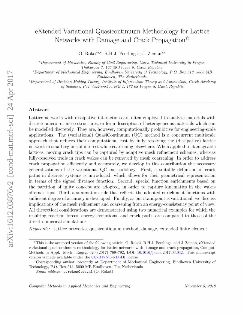
The problem of interest in this contribution is the combination of the QC method andcrack propagation in damageable lattice structures, as depicted in Fig. 1. Because most ofthe dissipation and fibre reorientation occurs near the crack tip, this region must be fullyresolved. To this end, a mesh indicator that follows the evolution of the crack tip needs to beprovided. Such an approach typically leaves a trail of the fully resolved region in the wakeof the crack, cf. Rokos et al. (2017). It may be clear that, apart from allowing the crack toopen up, these fully resolved regions do not contribute to the overall physics and accuracy.It is therefore desirable to coarsen them. However, this coarsening should take into accountthe effect which the crack has on the local, coarse-scale kinematics of the problem—i.e. itshould allow an arbitrary amount of crack opening without any mechanical resistance.

2

Fully resolvedcrack wake

Damaged bonds

Interpolationelement

Fully resolvedprocess zone

Underlyinglattice model

Figure 1: Sketch of a crack propagating in a damageable lattice using an adaptive QC method that onlyincludes mesh refinement. The lattice at the crack tip is fully resolved because large fibre deformationsand dissipation occur there. Elsewhere, the displacements are locally homogeneous and no damage occurs,allowing for efficient coarsening and large elements.

The aim of this contribution is to develop an extended version of the variational QCmethodology, building thereby an efficient approach to model ”strong discontinuities” indiscrete systems with fully-nonlocal representations. This is possible because the damagein the crack wake is highly localized, and can be treated as a ”discontinuity”, although thesystem itself is fully discrete. One can introduce, therefore, techniques known from the Ex-tended Finite Element Method (XFEM), (Belytschko and Black, 1999; Moes et al., 1999), orGeneralized Finite Element Method (GFEM), (Strouboulis et al., 2000a,b), that rely on thePartition of Unity (PU) concept (Melenk and Babuska, 1996; Babuska and Melenk, 1997). Inparticular, the space of interpolation functions is enriched to include jumps in the kinematicsas well as in the internal variables. Such an enrichment requires the development of severaltheoretical concepts and generalizations to our previous adaptive version of the variationalQC methodology Rokos et al. (2017), which was designed for materials with a higher de-gree of distributed cracking where effective coarsening is not possible. First, an appropriategeometric definition of crack path, identified through the state variable of a lattice system,is required. Second, cracks are geometrically described in terms of the level set function,which in turn provides the means to build special enrichments capturing the kinematics inthe wakes of cracks. In order to sample the incremental energy of the system accurately, asuitable summation rule needs to be provided. Finally, to obtain energy-consistent solutions,certain energy quantities must be treated in a special way due to the coarsening. As willbe explained below, and demonstrated in the examples section, the developed methodologyoffers an accurate yet efficient framework to model cracks in damageable lattices. In whatfollows, this approach will be referred to as the eXtended QC (in analogy to continuumsystems), or X-QC for short.

Several previous works have focused on generalizations of the QC methodology incorpo-rating XFEM-type of enrichments as well, cf. Gracie and Belytschko (2009); Aubertin et al.(2009, 2010); Talebi et al. (2013). Nevertheless, these works mainly dealt with conservativeatomistic lattice models within the scope of molecular dynamics and the bridging domainmethod (concurrent coupling between the atomistic and continuum regions). In contrast tothese previous works, this contribution focuses on dissipative QC methodologies, specifically

3

designed for dissipative structural lattice networks at the meso-scale level. Moreover, ourapproach relies on the fully non-local formulation, meaning that no continuum is used andthat the developed framework is fully discrete.

The paper is organized as follows. In Section 2, we briefly recall the theory of rate-independent systems on which the variational QC is built. For simplicity, only time-discreteversions of all equations are provided. Having specified the theoretical background, wecan introduce the model at hand, its geometry, state variables, and energies driving theevolution. For simplicity, our considerations are confined to 2D, although entire frameworkextends to 3D as well. The main developments of this contribution, i.e. the interpolation andsummation QC steps revisited from the point of view of lattice structures with propagatingcracks, are discussed in Section 3. In particular, the enrichment functions together with therequired changes in the summation rule are introduced in detail. The numerical solution ofthe resulting governing equations is not discussed as it can be found elsewhere, cf. Rokoset al. (2017), Section 4. Instead, we directly proceed to examples in Section 4, where theadditional efficiency of the proposed methodology is demonstrated. The results show thatthe X-QC approach allows one to reduce the number of DOFs to approximately 25 – 75 % ofthat of an adaptive QC, with no significant increase in error. The number of DOFs reduces to1 – 15 % of that of the Direct Numerical Simulations (DNS). The corresponding computingtimes are reduced by a factor of 4 – 20, depending on the particular example. The papercloses with a summary and conclusions in Section 5.

2. Variational Formulation of Lattice Networks with Localized Damage

In this section, the basic principles of the variational formulation of rate-independent sys-tems in the context of lattice networks are recalled. For the sake of brevity, we limit ourselvesto the time-discrete setting; the general theory is discussed in Mielke and Roubıcek (2015),whereas applications to continuous systems can be found, e.g., in Muhlhaus and Aifantis(1991); Han and Reddy (1995); Bourdin et al. (2000); Mielke et al. (2002); Mielke (2003);Bourdin (2007); Bourdin et al. (2008); Burke et al. (2010); Pham et al. (2011); Hofacker andMiehe (2012); Jirasek and Zeman (2015); Mesgarnejad et al. (2015). Applications to latticenetworks and QC are presented in Rokos et al. (2016, 2017) for isotropic hardening plasticityand localized damage, respectively.

2.1. General Considerations

An admissible configuration of a rate-independent system of interest is specified by astate variable q = (r, z), where r stores the kinematic variables and z the internal variables.All admissible configurations are specified by the state space Q = R ×Z , r ∈ R, z ∈ Z ,which incorporates, e.g., prescribed displacements or constraints on damage variables.

The energetic solution q is determined using the following incremental minimizationproblem at time tk

q(tk) ∈ arg minq∈Q

Πk(q; q(tk−1)), k = 1, . . . , nT , (IP)

4

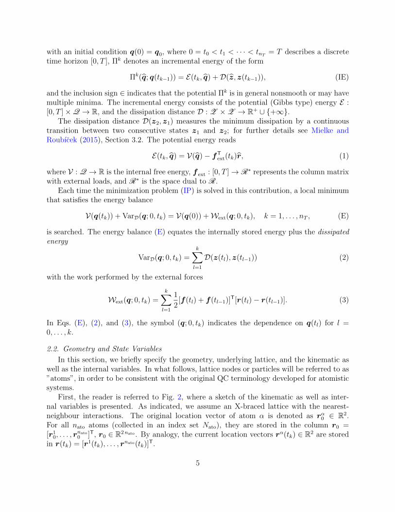
with an initial condition q(0) = q0, where 0 = t0 < t1 < · · · < tnT = T describes a discretetime horizon [0, T ], Πk denotes an incremental energy of the form

Πk(q; q(tk−1)) = E(tk, q) +D(z, z(tk−1)), (IE)

and the inclusion sign ∈ indicates that the potential Πk is in general nonsmooth or may havemultiple minima. The incremental energy consists of the potential (Gibbs type) energy E :[0, T ]×Q → R, and the dissipation distance D : Z ×Z → R+ ∪ +∞.

The dissipation distance D(z2, z1) measures the minimum dissipation by a continuoustransition between two consecutive states z1 and z2; for further details see Mielke andRoubıcek (2015), Section 3.2. The potential energy reads

E(tk, q) = V(q)− fText(tk)r, (1)

where V : Q → R is the internal free energy, f ext : [0, T ]→ R∗ represents the column matrixwith external loads, and R∗ is the space dual to R.

Each time the minimization problem (IP) is solved in this contribution, a local minimumthat satisfies the energy balance

V(q(tk)) + VarD(q; 0, tk) = V(q(0)) +Wext(q; 0, tk), k = 1, . . . , nT , (E)

is searched. The energy balance (E) equates the internally stored energy plus the dissipatedenergy

VarD(q; 0, tk) =k∑l=1

D(z(tl), z(tl−1)) (2)

with the work performed by the external forces

Wext(q; 0, tk) =k∑l=1

1

2[f(tl) + f(tl−1)]

T[r(tl)− r(tl−1)]. (3)

In Eqs. (E), (2), and (3), the symbol (q; 0, tk) indicates the dependence on q(tl) for l =0, . . . , k.

2.2. Geometry and State Variables

In this section, we briefly specify the geometry, underlying lattice, and the kinematic aswell as the internal variables. In what follows, lattice nodes or particles will be referred to as”atoms”, in order to be consistent with the original QC terminology developed for atomisticsystems.

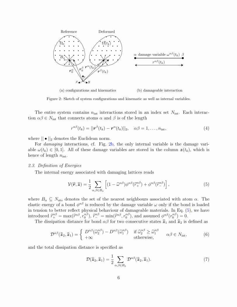
First, the reader is referred to Fig. 2, where a sketch of the kinematic as well as inter-nal variables is presented. As indicated, we assume an X-braced lattice with the nearest-neighbour interactions. The original location vector of atom α is denoted as rα0 ∈ R2.For all nato atoms (collected in an index set Nato), they are stored in the column r0 =[r1

0, . . . , rnato0 ]T, r0 ∈ R2nato . By analogy, the current location vectors rα(tk) ∈ R2 are stored

in r(tk) = [r1(tk), . . . , rnato(tk)]

T.

5

rβ(tk)rα(tk)rβ0rα0

zyx

Ω(tk)

Bα

Ω0

DeformedReference

(a) configurations and kinematics

damage variable ωαβ(tk)

rαβ(tk)

βα

(b) damageable interaction

Figure 2: Sketch of system configurations and kinematic as well as internal variables.

The entire system contains nint interactions stored in an index set Nint. Each interac-tion αβ ∈ Nint that connects atoms α and β is of the length

rαβ(tk) = ||rβ(tk)− rα(tk)||2, αβ = 1, . . . , nint, (4)

where || • ||2 denotes the Euclidean norm.For damaging interactions, cf. Fig. 2b, the only internal variable is the damage vari-

able ω(tk) ∈ [0, 1]. All of these damage variables are stored in the column z(tk), which ishence of length nint.

2.3. Definition of Energies

The internal energy associated with damaging lattices reads

V(r, z) =1

2

∑α,β∈Bα

[(1− ωαβ)φαβ(rαβ+ ) + φαβ(rαβ− )

], (5)

where Bα ⊆ Nato denotes the set of the nearest neighbours associated with atom α. Theelastic energy of a bond φαβ is reduced by the damage variable ω only if the bond is loadedin tension to better reflect physical behaviour of damageable materials. In Eq. (5), we haveintroduced rαβ+ = max(rαβ, rαβ0 ), rαβ− = min(rαβ, rαβ0 ), and assumed φαβ(rαβ0 ) = 0.

The dissipation distance for bond αβ for two consecutive states z1 and z2 is defined as

Dαβ(z2, z1) =

Dαβ(ωαβ2 )−Dαβ(ωαβ1 ) if ωαβ2 ≥ ωαβ1+∞ otherwise,

αβ ∈ Nint, (6)

and the total dissipation distance is specified as

D(z2, z1) =1

2

∑α,β∈Bα

Dαβ(z2, z1). (7)

6

In definition (6), Dαβ(ωαβ) is the energy dissipation of a single bond during a unidirectionaldamage process up to a damage level ωαβ. This function therefore increases from Dαβ(0) = 0to Dαβ(1) = gf,∞, where gf,∞ is the energy dissipated at complete failure.

The incremental interaction energy, πkαβ, and incremental site energy, πkα, then read:

πkαβ(q; q(tk−1)) = (1− ωαβ)φαβ(rαβ+ ) + φαβ(rαβ− ) +Dαβ(ωαβ, ωαβ(tk−1)), αβ = 1, . . . , nint,

(8a)

πkα(q; q(tk−1)) =1

2

∑β∈Bα

πkαβ(q, q(tk−1)), α = 1, . . . , nato. (8b)

3. Variational Quasicontinuum Methodology with Refinement and Coarsening

In this section we specify the two steps of the standard QC methodology, interpolationand summation, as well as additional procedures that must be adopted to extend it to anefficient description for localized damage. We start with a geometric crack description forlattice systems in Section 3.1, proceeding to the interpolation step in Section 3.2, where thestandard framework as well as the mesh refinement and the mesh coarsening are treated. Thefirst part closes with the description of the enrichment functions. The second part is devotedto summation, starting with the standard framework in Section 3.3, which is later extendedto incorporate also the enrichment functions. Finally, the complete X-QC procedure issummarized in Section 3.4 in terms of a general algorithm, and energy implications arediscussed in Section 3.5 in order to allow for proper verification of the energy equality (E).

3.1. Description of a Crack

In what follows, a crack is defined as an ordered set of points collected in a set C, cf.also Fries and Baydoun (2012):

If ωαβ ≥ η then1

2(rα0 + rβ0 ) ∈ C, and α, β ∈ Ncw. (9)

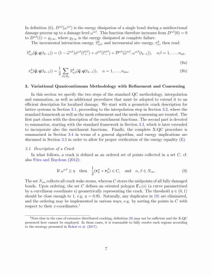
The setNcw collects all crack wake atoms, whereas C stores the midpoints of all fully damagedbonds. Upon ordering, the set C defines an oriented polygon ΓC(s) (a curve parametrizedby a curvilinear coordinate s) geometrically representing the crack. The threshold η ∈ (0, 1)should be close enough to 1, e.g. η = 0.95. Naturally, any duplicates in (9) are eliminated,and the ordering may be implemented in various ways, e.g. by sorting the points in C withrespect to their x-coordinates.1

1Note that in the case of extensive distributed cracking, definition (9) may not be sufficient and the X-QCpresented here cannot be employed. In those cases, it is reasonable to fully resolve such regions accordingto the strategy presented in Rokos et al. (2017).

7

z

y

x

rα0 − cα

rα0cα

tcα

ncα

s

ΓC(s)

33

3

22

2 11

1

000

-1-1

-1

-2-2

-2

-3-3

-3

Figure 3: Representation of an existing crack in a discrete lattice network. Damaged bonds (for which ωαβ ≥η, cf. definition (9)) are depicted by red lines (other interactions are omitted for clarity) and set C is depictedusing green dots. The signed distance function ψ is represented by contour lines, and the crack polygon ΓCis presented as a green line. Atom sites are shown as black dots.

For future use, it is convenient to introduce the signed distance function ψ, cf. e.g. Friesand Belytschko (2010), Section 3. Its definition reads

cα = arg minc∈ΓC

||rα0 − c||,

ψ(rα0 ) = ||rα0 − cα|| · sign(nTcα(rα0 − cα)),

α ∈ Nato, (10)

where ncα denotes the column storing the unit normal to the crack ΓC at the closest point cα.For instance, ncα can be defined such that tcα × ncα = ez, where tcα is the unit tangentvector to ΓC at cα, and ez is the unit basis vector pointing in the z-direction of the adoptedcoordinate system. If cα is situated at a kink of ΓC , entire cone of normals must be consid-ered; then, the sign of ψ(rα0 ) is positive if the vector rα0 − cα belongs to the cone of normalsand negative otherwise. The function ψ is therefore positive on one side of the crack andnegative on the other. Because the crack tip is always located inside the fully refined region,no second level set function is required to describe the crack tip, cf. Fries and Belytschko(2010), Section 3.2. For a pictorial representation of the introduced quantities see Fig. 3.

Within the X-QC framework, crack path bifurcations are included automatically as aresult of the full refinement in the process zone. Subsequent coarsening in the wakes ofcracks through special function enrichments would require further development. Becausecrack branching designed for continuous systems is rather technical, see e.g. Daux et al.(2000), one can expect a similar degree of technical complexity also for discrete systems.These kinds of generalizations lie outside the scope of the current manuscript and are leftas possible future challenges. Only isolated cracks are treated in the remainder of thismanuscript.

3.2. Interpolation

In the four following subsections, the interpolation step of the QC method and its effecton the incremental energy of the full system (Πk in (IE)) are detailed.

8

3.2.1. General Framework

Interpolation introduces to the minimization problem (IP) the following equality con-straints:

r = Φg, for g ∈ G (tk), (11)

where g denotes a column of generalized DOFs located in a kinematically constrained sub-space G (tk) of the fully dimensional space R(tk).

After substitution of Eq. (11), the incremental energy (IE) becomes a function of g, i.e.

Πk(r, z; r(tk−1), z(tk−1)) = Πk(Φg, z; Φg(tk−1), z(tk−1)), (12)

which can be minimized over the linear subspace G (tk). This reduces the computationaleffort if dim(G (tk)) dim(R(tk)).

In QC approaches, the generalised DOFs g are chosen as the DOFs of a small set ofatoms, the so-called repatoms. Usually, repatoms are chosen as nodes of a mesh T thattriangulates the domain Ω0, and the interpolation is implemented via piecewise affine (P1)FE shape functions constructed between the repatoms. Consequently, Φ contains standardFEM shape function evaluations at all atom positions, cf. e.g. Tadmor and Miller (2011).Note that higher-order polynomial approximations inside elements can be adopted as well,see e.g. Beex et al. (2014a), Yang and To (2015), or Beex et al. (2015b).

In order to distinguish classical QC approach from its extended version presented below,we use the following notation for the classical QC: all nrep repatoms are collected in an indexset Nrep ⊆ Nato, whereas their admissible positions rαrep ∈ R2, α ∈ Nrep, are stored in thecolumn rrep ∈ Rrep(tk) by analogy to r. Associated interpolation matrix is denoted ΦFE.

3.2.2. Mesh Refinement

In this contribution, the mesh refinement indicator of Rokos et al. (2017), is adoptedwith minor changes. It proceeds as follows: a triangle K of the current triangulation Tk isendowed with a set of sampling interactions SKint specified as

SKint stores those interactions αβ ∈ Sint for which1

2(rα + rβ) ∈ K.2 (13)

Then, the following energy condition is introduced

(1− ωαβ)φαβ(rαβ+ ) ≥ θr φαβth , αβ ∈ SKint, θr ∈ (0, 1), (14)

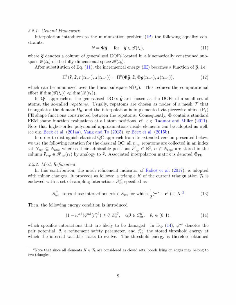
which specifies interactions that are likely to be damaged. In Eq. (14), φαβ denotes thepair potential, θr a refinement safety parameter, and φαβth the stored threshold energy atwhich the internal variable starts to evolve. The threshold energy is therefore obtained

2Note that since all elements K ∈ Tk are considered as closed sets, bonds lying on edges may belong totwo triangles.

9

as φαβth = φαβ(r0(1 + ε0)), where ε0 is the limit elastic strain, one of the input parameters ofthe employed constitutive model, see Tab. 1. The mesh refinement indicator then reads

If condition (14) holds at least for one interaction αβ ∈ SKint=⇒ mark K for refinement, i.e. add K to Ir.

(15)

Having specified a set of triangles marked for refinement, Ir ⊆ Tk, the current trian-gulation Tk must be refined. To this end, the backward-longest-edge-bisection algorithmby Rivara (1997) is used.

3.2.3. Mesh Coarsening

Before coarsening the current triangulation Tk, first an indicator is presented that markswhich triangles need to be coarsened. In analogy to Eq. (14) we introduce the followingenergy condition

(1− ωαβ)φαβ(rαβ+ ) + φαβ(rαβ− ) ≤ θc φαβth , αβ ∈ SKint, θc ∈ (0, 1), θc < θr, (16)

where the compressive part is now included as well. The rationale behind condition (16) isthat in the crack wake the stress is low, and hence also the energy. The mesh coarseningindicator then reads

If condition (16) holds for all interactions αβ ∈ SKint=⇒ mark K for coarsening, i.e. add K to Ic.

(17)

Verifying condition (17) for all elements yields a set of triangles marked for coarsening,Ic ⊆ Tk.

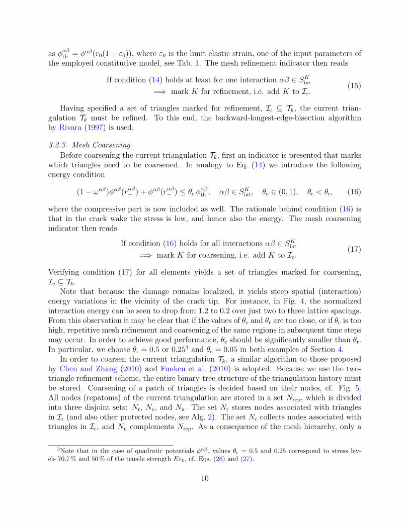
Note that because the damage remains localized, it yields steep spatial (interaction)energy variations in the vicinity of the crack tip. For instance, in Fig. 4, the normalizedinteraction energy can be seen to drop from 1.2 to 0.2 over just two to three lattice spacings.From this observation it may be clear that if the values of θc and θr are too close, or if θc is toohigh, repetitive mesh refinement and coarsening of the same regions in subsequent time stepsmay occur. In order to achieve good performance, θc should be significantly smaller than θr.In particular, we choose θr = 0.5 or 0.253 and θc = 0.05 in both examples of Section 4.

In order to coarsen the current triangulation Tk, a similar algorithm to those proposedby Chen and Zhang (2010) and Funken et al. (2010) is adopted. Because we use the two-triangle refinement scheme, the entire binary-tree structure of the triangulation history mustbe stored. Coarsening of a patch of triangles is decided based on their nodes, cf. Fig. 5.All nodes (repatoms) of the current triangulation are stored in a set Nrep, which is dividedinto three disjoint sets: Nr, Nc, and Nu. The set Nr stores nodes associated with trianglesin Ir (and also other protected nodes, see Alg. 2). The set Nc collects nodes associated withtriangles in Ic, and Nu complements Nrep. As a consequence of the mesh hierarchy, only a

3Note that in the case of quadratic potentials φαβ , values θr = 0.5 and 0.25 correspond to stress lev-els 70.7 % and 50 % of the tensile strength Eε0, cf. Eqs. (26) and (27).

10

0.2

0.4

0.6

0.8

1

1.2

Figure 4: An example of contours of normalized energy φαβ/φαβth around a crack tip (based on linearlyinterpolated data) of a QC system. Regular atom sites are shown as black dots and the existing crack as agreen line.

X: 64Y: 48

000 001 002 003 004 005 006 007008

009

010

011

012

013

014

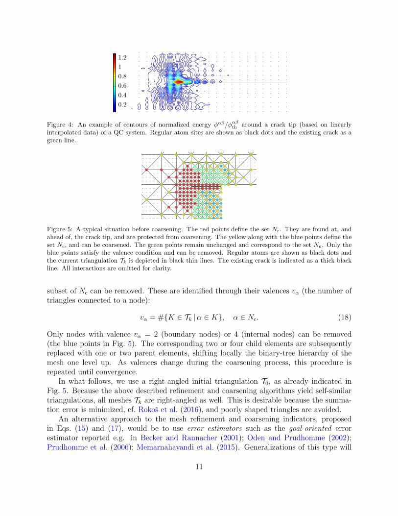
Figure 5: A typical situation before coarsening. The red points define the set Nr. They are found at, andahead of, the crack tip, and are protected from coarsening. The yellow along with the blue points define theset Nc, and can be coarsened. The green points remain unchanged and correspond to the set Nu. Only theblue points satisfy the valence condition and can be removed. Regular atoms are shown as black dots andthe current triangulation Tk is depicted in black thin lines. The existing crack is indicated as a thick blackline. All interactions are omitted for clarity.

subset of Nc can be removed. These are identified through their valences vα (the number oftriangles connected to a node):

vα = #K ∈ Tk |α ∈ K, α ∈ Nc. (18)

Only nodes with valence vα = 2 (boundary nodes) or 4 (internal nodes) can be removed(the blue points in Fig. 5). The corresponding two or four child elements are subsequentlyreplaced with one or two parent elements, shifting locally the binary-tree hierarchy of themesh one level up. As valences change during the coarsening process, this procedure isrepeated until convergence.

In what follows, we use a right-angled initial triangulation T0, as already indicated inFig. 5. Because the above described refinement and coarsening algorithms yield self-similartriangulations, all meshes Tk are right-angled as well. This is desirable because the summa-tion error is minimized, cf. Rokos et al. (2016), and poorly shaped triangles are avoided.

An alternative approach to the mesh refinement and coarsening indicators, proposedin Eqs. (15) and (17), would be to use error estimators such as the goal-oriented errorestimator reported e.g. in Becker and Rannacher (2001); Oden and Prudhomme (2002);Prudhomme et al. (2006); Memarnahavandi et al. (2015). Generalizations of this type will

11

0 10 20 30 40 50 60 700

10

20

30

40

50

60

(a) reproducing and blending ele-ments

12 sign(ψ(r0))

−1/2

+1/2

(b) enrichment function, 12 sign(ψ(r0))

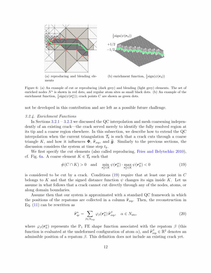
Figure 6: (a) An example of cut or reproducing (dark grey) and blending (light grey) elements. The set ofenriched nodes N? is shown in red dots, and regular atom sites as small black dots. (b) An example of theenrichment function, 1

2 sign(ψ(rα0 )); crack points C are shown as green dots.

not be developed in this contribution and are left as a possible future challenge.

3.2.4. Enrichment Functions

In Sections 3.2.1 – 3.2.3 we discussed the QC interpolation and mesh coarsening indepen-dently of an existing crack—the crack served merely to identify the fully resolved region atits tip and a coarse region elsewhere. In this subsection, we describe how to extend the QCinterpolation when the current triangulation Tk is such that a crack cuts through a coarsetriangle K, and how it influences Φ, rrep, and g. Similarly to the previous sections, thediscussion considers the system at time step tk.

We first specify the cut elements (also called reproducing, Fries and Belytschko 2010),cf. Fig. 6a. A coarse element K ∈ Tk such that

#(C ∩K) > 0 and minrα0∈K

ψ(rα0 ) · maxrα0∈K

ψ(rα0 ) < 0 (19)

is considered to be cut by a crack. Conditions (19) require that at least one point in Cbelongs to K and that the signed distance function ψ changes its sign inside K. Let usassume in what follows that a crack cannot cut directly through any of the nodes, atoms, oralong domain boundaries.

Assume then that our system is approximated with a standard QC framework in whichthe positions of the repatoms are collected in a column rrep. Then, the reconstruction inEq. (11) can be rewritten as

rαqc =∑β∈Nrep

ϕβ(rα0 ) rβrep, α ∈ Nato, (20)

where ϕβ(rα0 ) represents the P1 FE shape function associated with the repatom β (this

function is evaluated at the undeformed configuration of atom α), and rβrep ∈ R2 denotes anadmissible position of a repatom β. This definition does not include an existing crack yet.

12

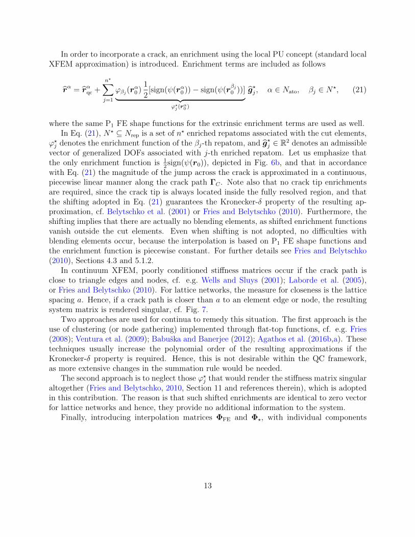
In order to incorporate a crack, an enrichment using the local PU concept (standard localXFEM approximation) is introduced. Enrichment terms are included as follows

rα = rαqc +n?∑j=1

ϕβj(rα0 )

1

2[sign(ψ(rα0 ))− sign(ψ(r

βj0 ))]︸ ︷︷ ︸

ϕ?j (rα0 )

g?j , α ∈ Nato, βj ∈ N?, (21)

where the same P1 FE shape functions for the extrinsic enrichment terms are used as well.In Eq. (21), N? ⊆ Nrep is a set of n? enriched repatoms associated with the cut elements,

ϕ?j denotes the enrichment function of the βj-th repatom, and g?j ∈ R2 denotes an admissiblevector of generalized DOFs associated with j-th enriched repatom. Let us emphasize thatthe only enrichment function is 1

2sign(ψ(r0)), depicted in Fig. 6b, and that in accordance

with Eq. (21) the magnitude of the jump across the crack is approximated in a continuous,piecewise linear manner along the crack path ΓC . Note also that no crack tip enrichmentsare required, since the crack tip is always located inside the fully resolved region, and thatthe shifting adopted in Eq. (21) guarantees the Kronecker-δ property of the resulting ap-proximation, cf. Belytschko et al. (2001) or Fries and Belytschko (2010). Furthermore, theshifting implies that there are actually no blending elements, as shifted enrichment functionsvanish outside the cut elements. Even when shifting is not adopted, no difficulties withblending elements occur, because the interpolation is based on P1 FE shape functions andthe enrichment function is piecewise constant. For further details see Fries and Belytschko(2010), Sections 4.3 and 5.1.2.

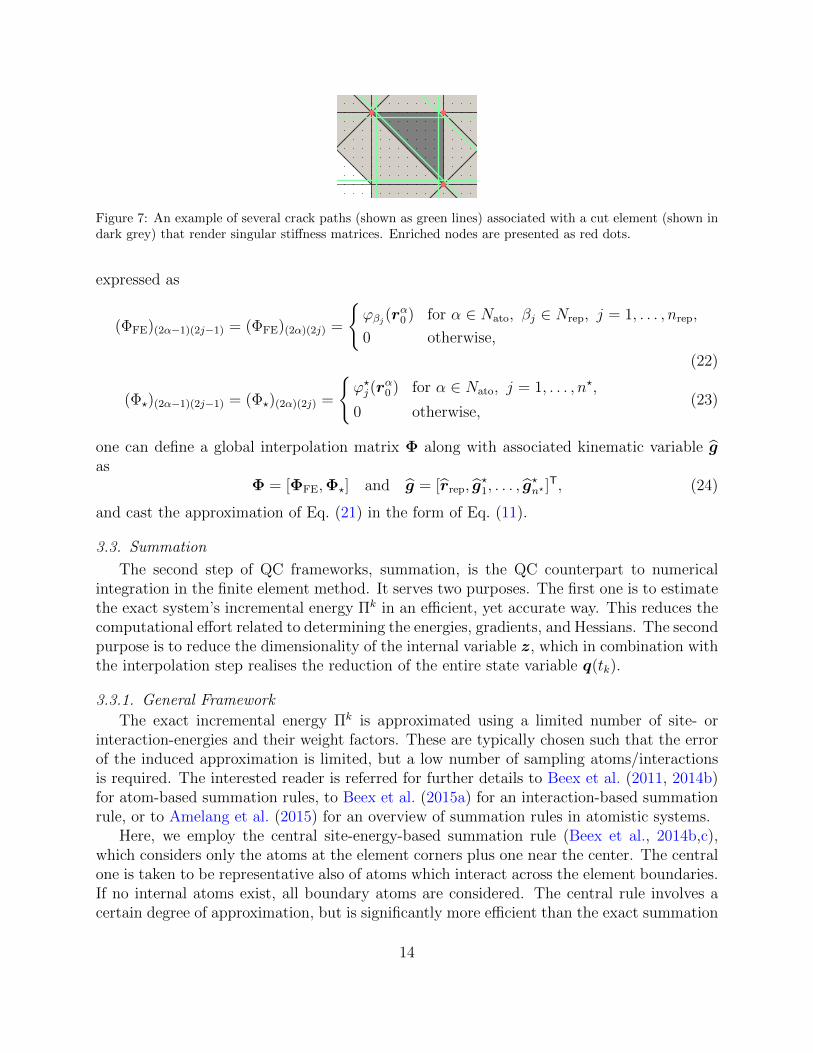
In continuum XFEM, poorly conditioned stiffness matrices occur if the crack path isclose to triangle edges and nodes, cf. e.g. Wells and Sluys (2001); Laborde et al. (2005),or Fries and Belytschko (2010). For lattice networks, the measure for closeness is the latticespacing a. Hence, if a crack path is closer than a to an element edge or node, the resultingsystem matrix is rendered singular, cf. Fig. 7.

Two approaches are used for continua to remedy this situation. The first approach is theuse of clustering (or node gathering) implemented through flat-top functions, cf. e.g. Fries(2008); Ventura et al. (2009); Babuska and Banerjee (2012); Agathos et al. (2016b,a). Thesetechniques usually increase the polynomial order of the resulting approximations if theKronecker-δ property is required. Hence, this is not desirable within the QC framework,as more extensive changes in the summation rule would be needed.

The second approach is to neglect those ϕ?j that would render the stiffness matrix singularaltogether (Fries and Belytschko, 2010, Section 11 and references therein), which is adoptedin this contribution. The reason is that such shifted enrichments are identical to zero vectorfor lattice networks and hence, they provide no additional information to the system.

Finally, introducing interpolation matrices ΦFE and Φ?, with individual components

13

10 15 20 25 3020

25

30

35

40

Figure 7: An example of several crack paths (shown as green lines) associated with a cut element (shown indark grey) that render singular stiffness matrices. Enriched nodes are presented as red dots.

expressed as

(ΦFE)(2α−1)(2j−1) = (ΦFE)(2α)(2j) =

ϕβj(r

α0 ) for α ∈ Nato, βj ∈ Nrep, j = 1, . . . , nrep,

0 otherwise,

(22)

(Φ?)(2α−1)(2j−1) = (Φ?)(2α)(2j) =

ϕ?j(r

α0 ) for α ∈ Nato, j = 1, . . . , n?,

0 otherwise,(23)

one can define a global interpolation matrix Φ along with associated kinematic variable gas

Φ = [ΦFE,Φ?] and g = [rrep, g?1, . . . , g

?n? ]

T, (24)

and cast the approximation of Eq. (21) in the form of Eq. (11).

3.3. Summation

The second step of QC frameworks, summation, is the QC counterpart to numericalintegration in the finite element method. It serves two purposes. The first one is to estimatethe exact system’s incremental energy Πk in an efficient, yet accurate way. This reduces thecomputational effort related to determining the energies, gradients, and Hessians. The secondpurpose is to reduce the dimensionality of the internal variable z, which in combination withthe interpolation step realises the reduction of the entire state variable q(tk).

3.3.1. General Framework

The exact incremental energy Πk is approximated using a limited number of site- orinteraction-energies and their weight factors. These are typically chosen such that the errorof the induced approximation is limited, but a low number of sampling atoms/interactionsis required. The interested reader is referred for further details to Beex et al. (2011, 2014b)for atom-based summation rules, to Beex et al. (2015a) for an interaction-based summationrule, or to Amelang et al. (2015) for an overview of summation rules in atomistic systems.

Here, we employ the central site-energy-based summation rule (Beex et al., 2014b,c),which considers only the atoms at the element corners plus one near the center. The centralone is taken to be representative also of atoms which interact across the element boundaries.If no internal atoms exist, all boundary atoms are considered. The central rule involves acertain degree of approximation, but is significantly more efficient than the exact summation

14

rule not discussed here; for details see (Beex et al., 2011). The summation rule is implementedby introducing a set of nato

sam sampling atoms collected in an index set Sato ⊆ Nato. The nintsam

interactions connected to these sampling atoms are stored in an index set Sint. Then, thesummation step yields the following approximation,

Πk(q; q(tk−1)) ≈ Πk(q; q(tk−1)) =∑α∈Sato

wαπkα(q; q(tk−1))− fT

extr

=∑

αβ∈Sint

wαβπkαβ(q; q(tk−1))− fT

extr,(25)

where wα are the weight factors associated with atom sites, and wαβ are corresponding weightfactors associated with interactions.

Because the approximate incremental energy in Eq. (25) only depends on the internalvariables associated with nint

sam interactions, one can introduce a reduced state variable of theQC system in the form qred(tk) = (g(tk), zsam(tk)) ∈ Qred(tk), where zsam ∈ Rnint

sam = Zsam isa column that stores the internal variables of all sampling interactions. The reduced statespace then reads Qred(tk) = G (tk)×Zsam.

3.3.2. Summation Rule for Enrichment Functions

If the enrichment of Section 3.2.4 is adopted and a coarse triangle is cut by a crack,Eq. (25) still holds, but the selection of the individual sampling atoms Sato and theirweights wα changes.

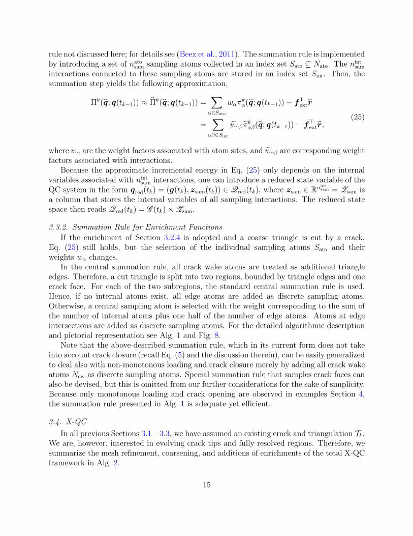
In the central summation rule, all crack wake atoms are treated as additional triangleedges. Therefore, a cut triangle is split into two regions, bounded by triangle edges and onecrack face. For each of the two subregions, the standard central summation rule is used.Hence, if no internal atoms exist, all edge atoms are added as discrete sampling atoms.Otherwise, a central sampling atom is selected with the weight corresponding to the sum ofthe number of internal atoms plus one half of the number of edge atoms. Atoms at edgeintersections are added as discrete sampling atoms. For the detailed algorithmic descriptionand pictorial representation see Alg. 1 and Fig. 8.

Note that the above-described summation rule, which in its current form does not takeinto account crack closure (recall Eq. (5) and the discussion therein), can be easily generalizedto deal also with non-monotonous loading and crack closure merely by adding all crack wakeatoms Ncw as discrete sampling atoms. Special summation rule that samples crack faces canalso be devised, but this is omitted from our further considerations for the sake of simplicity.Because only monotonous loading and crack opening are observed in examples Section 4,the summation rule presented in Alg. 1 is adequate yet efficient.

3.4. X-QC

In all previous Sections 3.1 – 3.3, we have assumed an existing crack and triangulation Tk.We are, however, interested in evolving crack tips and fully resolved regions. Therefore, wesummarize the mesh refinement, coarsening, and additions of enrichments of the total X-QCframework in Alg. 2.

15

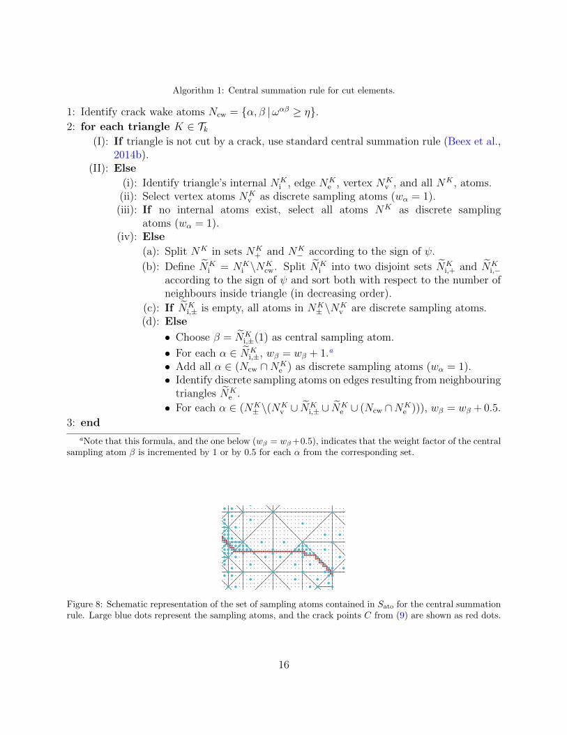
Algorithm 1: Central summation rule for cut elements.

1: Identify crack wake atoms Ncw = α, β |ωαβ ≥ η.2: for each triangle K ∈ Tk

(I): If triangle is not cut by a crack, use standard central summation rule (Beex et al.,2014b).

(II): Else

(i): Identify triangle’s internal NKi , edge NK

e , vertex NKv , and all NK , atoms.

(ii): Select vertex atoms NKv as discrete sampling atoms (wα = 1).

(iii): If no internal atoms exist, select all atoms NK as discrete samplingatoms (wα = 1).

(iv): Else

(a): Split NK in sets NK+ and NK

− according to the sign of ψ.

(b): Define NKi = NK

i \NKcw. Split NK

i into two disjoint sets NKi,+ and NK

i,−according to the sign of ψ and sort both with respect to the number ofneighbours inside triangle (in decreasing order).

(c): If NKi,± is empty, all atoms in NK

± \NKv are discrete sampling atoms.

(d): Else

• Choose β = NKi,±(1) as central sampling atom.

• For each α ∈ NKi,±, wβ = wβ + 1.a

• Add all α ∈ (Ncw ∩NKe ) as discrete sampling atoms (wα = 1).

• Identify discrete sampling atoms on edges resulting from neighbouringtriangles NK

e .

• For each α ∈ (NK± \(NK

v ∪ NKi,± ∪ NK

e ∪ (Ncw ∩NKe ))), wβ = wβ + 0.5.

3: end

aNote that this formula, and the one below (wβ = wβ+0.5), indicates that the weight factor of the centralsampling atom β is incremented by 1 or by 0.5 for each α from the corresponding set.

y

x

0 10 20 30 40 50 60 700

10

20

30

40

50

60

Figure 8: Schematic representation of the set of sampling atoms contained in Sato for the central summationrule. Large blue dots represent the sampling atoms, and the crack points C from (9) are shown as red dots.

16

Algorithm 2: X-QC algorithm.

1: Initialize the system: apply initial condition q0 and construct initial (coarse) mesh T0with required information, e.g. Nrep(t0), Φ(t0), Sato(t0), Sint(t0).

2: for k = 1, . . . , nT(i): Apply the boundary conditions at time tk, Tk = Tk−1, Nrep(tk) = Nrep(tk−1), Φ(tk) =

Φ(tk−1), Sato(tk) = Sato(tk−1), Sint(tk) = Sint(tk−1), etc.(ii): Equilibrate the unbalanced system, i.e. solve for qred(tk) ∈ Qred(tk) us-

ing Πk(qred; qred(tk−1)) of Eq. (25). Update crack description ψ, C, etc.(iii): For each coarse element K ∈ Tk evaluate its refinement indicator in (15) and con-

struct Ir ⊆ Tk. If Ir 6= ∅ refine and update Tk.(iv): Protect newly added repatoms from all previous refinements during the current

time step tk; if necessary, protect also other repatoms, e.g. those near the crack tip.Use (17) to identify Ic ⊆ Tk. If possible, coarsen and update Tk.

(v): If Tk changed in (iii) – (iv), update the system information Nrep(tk), Φ(tk), Sato(tk),Sint(tk), etc., and return to (ii) since the system is unbalanced.Else if the mesh has converged; proceed to (vi).

(vi): Store relevant outputs: qred(tk), Tk, Nrep(tk), Φ(tk), Sato(tk), Sint(tk), C, etc.

3: end

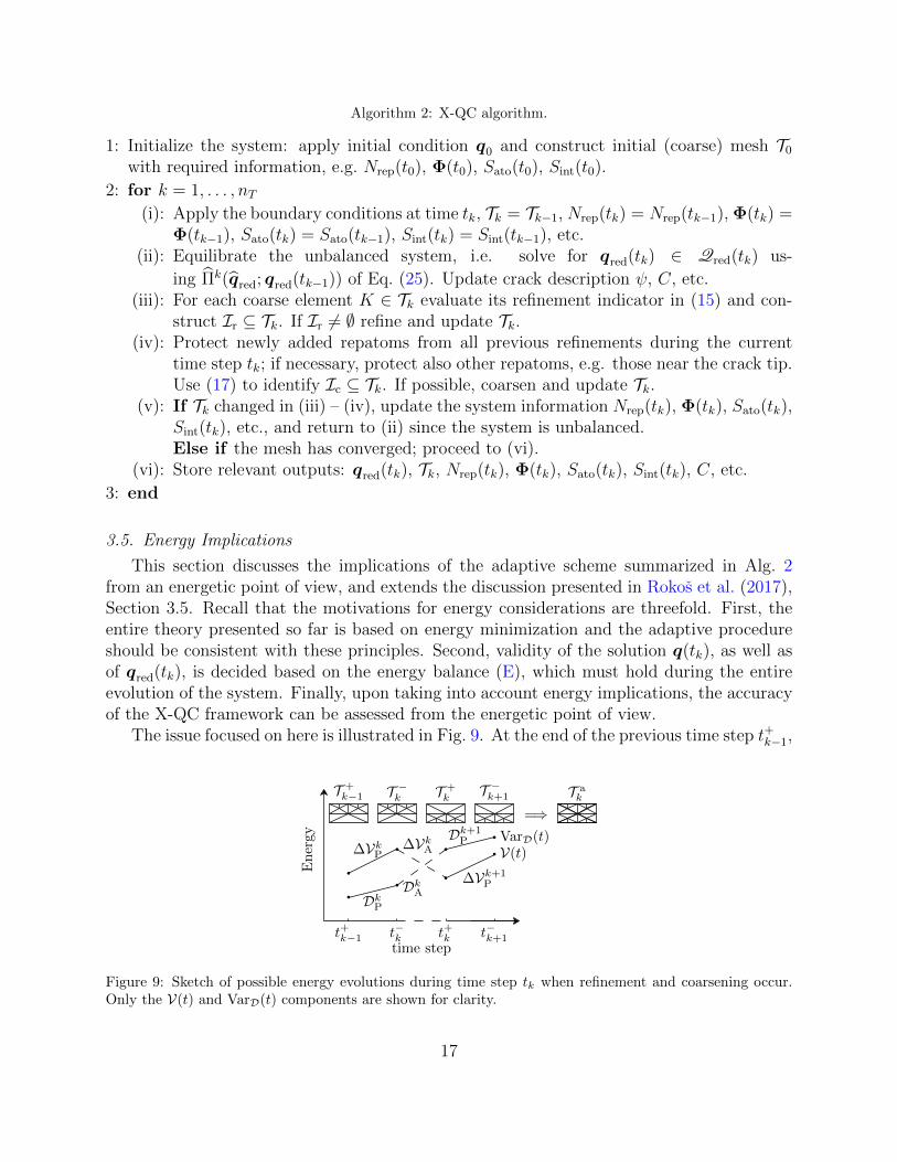
3.5. Energy Implications

This section discusses the implications of the adaptive scheme summarized in Alg. 2from an energetic point of view, and extends the discussion presented in Rokos et al. (2017),Section 3.5. Recall that the motivations for energy considerations are threefold. First, theentire theory presented so far is based on energy minimization and the adaptive procedureshould be consistent with these principles. Second, validity of the solution q(tk), as well asof qred(tk), is decided based on the energy balance (E), which must hold during the entireevolution of the system. Finally, upon taking into account energy implications, the accuracyof the X-QC framework can be assessed from the energetic point of view.

The issue focused on here is illustrated in Fig. 9. At the end of the previous time step t+k−1,

T ak

=⇒T −k+1T +

kT −k

T +k−1

VarD(t)V(t)

∆Vk+1P

Dk+1P

DkA

∆VkA

DkP

∆VkP

Energy

time stept−k+1t+kt−kt+k−1

Figure 9: Sketch of possible energy evolutions during time step tk when refinement and coarsening occur.Only the V(t) and VarD(t) components are shown for clarity.

17

the system is relaxed for some mesh T +k−1. After the next increment is applied for mesh T −k =

T +k−1 and the system is equilibrated (stage (ii) of Alg. 2), refinement and coarsening may be

required ((ii) – (iv)). Upon convergence, this yields a triangulation T +k . In order to accurately

construct the energy increments, one should distinguish physical increments, computed onmesh T +

k−1 and denoted with subscripts ”P”, and changes in energy which are due to the meshadaptation from T −k to T +

k , denoted with subscripts ”A”. The artificial energy incrementsdue to mesh adaptation are computed by projecting converged solutions onto an artificialmesh T a

k , which establishes communication between the two systems (note that these twosystems have different numbers of DOFs and internal variables). The artificial mesh thereforecontains the union of repatoms and sampling interactions present in both systems and hence,it is locally the finest triangulation of the two, cf. Fig. 9. Using the above-described procedureand evaluating energies at time instants t+k provides energy evolution paths that we will callreconstructed. For further details see Rokos et al. (2017), Section 3.5.

Let us note that we omit dissipative coarsening (i.e. the interpolation of the internalvariables when the mesh is coarsened), and assume that the coarsening occurs only in elas-tic regions. This assumption is reasonable because damage is localized. Consequently, alldamaged bonds are captured accurately by the special function enrichments and associatedsummation rule.

4. Numerical Examples

In this section the framework is applied to two examples discussed already in Rokoset al. (2017), where coarsening was not considered. Consequently, we can make a directcomparison in terms of accuracy and efficiency between the adaptive QC frameworks withand without coarsening.

The same material model is used for each lattice spring (the superscripts αβ are droppedfor brevity):

φ(r) =1

2EAr0(ε(r))

2, (26)

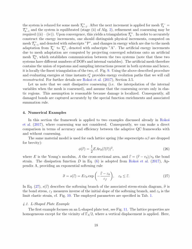
where E is the Young’s modulus, A the cross-sectional area, and ε = (r − r0)/r0 the bondstrain. The dissipation function D in Eq. (6) is adopted from Rokos et al. (2017), Ap-pendix A, providing an exponential softening rule

σ = s(ε) = Eε0 exp

(− ε− ε0

εf

), ε0 ≤ ε. (27)

In Eq. (27), s(ε) describes the softening branch of the associated stress-strain diagram, σ isthe bond stress, εf measures inverse of the initial slope of the softening branch, and ε0 is thelimit elastic strain, cf. Fig. 10. The employed parameters are specified in Tab. 1.

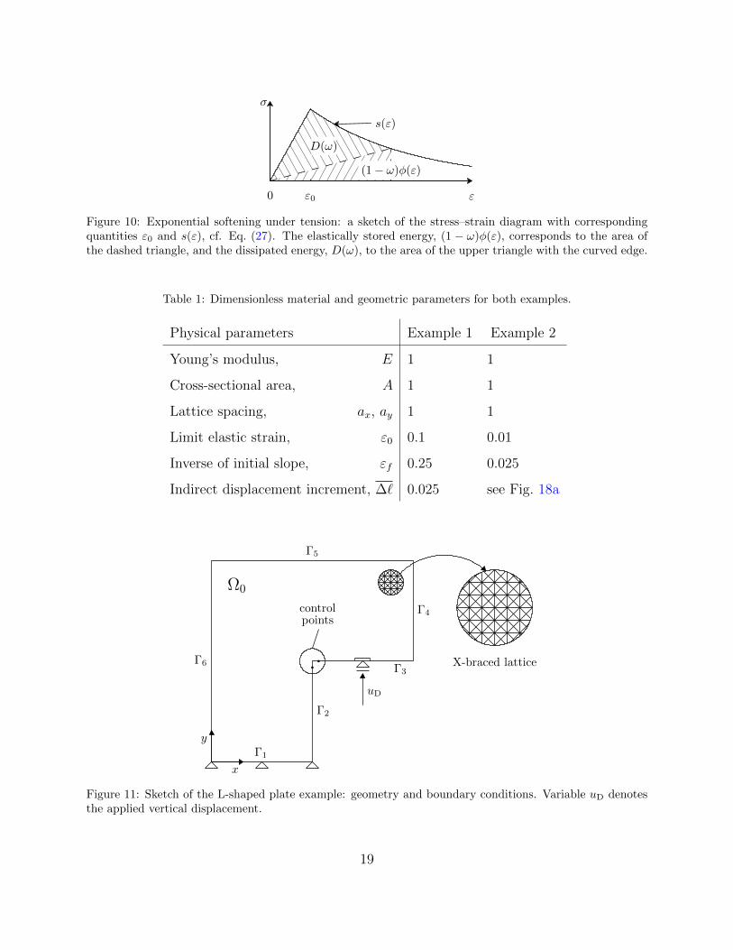
4.1. L-Shaped Plate Example

The first example focuses on an L-shaped plate test, see Fig. 11. The lattice properties arehomogeneous except for the vicinity of Γ3/2, where a vertical displacement is applied. Here,

18

D

ω

ω

ε

s(ε)

σ

ε

(1− ω)φ(ε)

D(ω)

0 1

0 ε0

0 ε0

gf,∞

1Figure 10: Exponential softening under tension: a sketch of the stress–strain diagram with correspondingquantities ε0 and s(ε), cf. Eq. (27). The elastically stored energy, (1 − ω)φ(ε), corresponds to the area ofthe dashed triangle, and the dissipated energy, D(ω), to the area of the upper triangle with the curved edge.

Table 1: Dimensionless material and geometric parameters for both examples.

Physical parameters Example 1 Example 2

Young’s modulus, E 1 1

Cross-sectional area, A 1 1

Lattice spacing, ax, ay 1 1

Limit elastic strain, ε0 0.1 0.01

Inverse of initial slope, εf 0.25 0.025

Indirect displacement increment, ∆` 0.025 see Fig. 18a

X-braced lattice

controlpoints

y

x

uD

Ω0

Γ6

Γ5

Γ4

Γ3

Γ2

Γ1

Figure 11: Sketch of the L-shaped plate example: geometry and boundary conditions. Variable uD denotesthe applied vertical displacement.

19

y

x

0 20 40 600

20

40

60

80

(a) r(tk) for uD = 14

prog. X-QCmod. X-QCDNSprog. ad. QCmod. ad. QC

F

uD

0 5 10 15 200

0.2

0.4

(b) force-displacement diagram

15.5 16 16.5

0.04

0.06

0.08 Zoom in

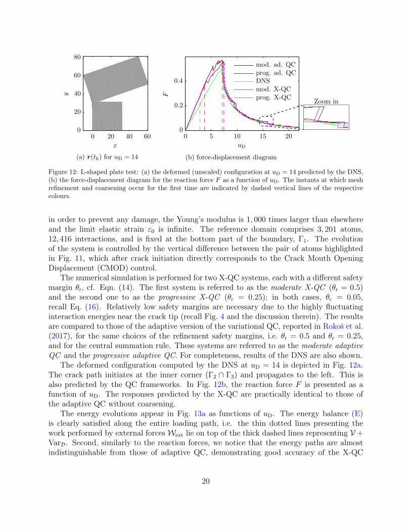
Figure 12: L-shaped plate test: (a) the deformed (unscaled) configuration at uD = 14 predicted by the DNS,(b) the force-displacement diagram for the reaction force F as a function of uD. The instants at which meshrefinement and coarsening occur for the first time are indicated by dashed vertical lines of the respectivecolours.

in order to prevent any damage, the Young’s modulus is 1, 000 times larger than elsewhereand the limit elastic strain ε0 is infinite. The reference domain comprises 3, 201 atoms,12, 416 interactions, and is fixed at the bottom part of the boundary, Γ1. The evolutionof the system is controlled by the vertical difference between the pair of atoms highlightedin Fig. 11, which after crack initiation directly corresponds to the Crack Mouth OpeningDisplacement (CMOD) control.

The numerical simulation is performed for two X-QC systems, each with a different safetymargin θr, cf. Eqn. (14). The first system is referred to as the moderate X-QC (θr = 0.5)and the second one to as the progressive X-QC (θr = 0.25); in both cases, θc = 0.05,recall Eq. (16). Relatively low safety margins are necessary due to the highly fluctuatinginteraction energies near the crack tip (recall Fig. 4 and the discussion therein). The resultsare compared to those of the adaptive version of the variational QC, reported in Rokos et al.(2017), for the same choices of the refinement safety margins, i.e. θr = 0.5 and θr = 0.25,and for the central summation rule. These systems are referred to as the moderate adaptiveQC and the progressive adaptive QC. For completeness, results of the DNS are also shown.

The deformed configuration computed by the DNS at uD = 14 is depicted in Fig. 12a.The crack path initiates at the inner corner (Γ2 ∩ Γ3) and propagates to the left. This isalso predicted by the QC frameworks. In Fig. 12b, the reaction force F is presented as afunction of uD. The responses predicted by the X-QC are practically identical to those ofthe adaptive QC without coarsening.

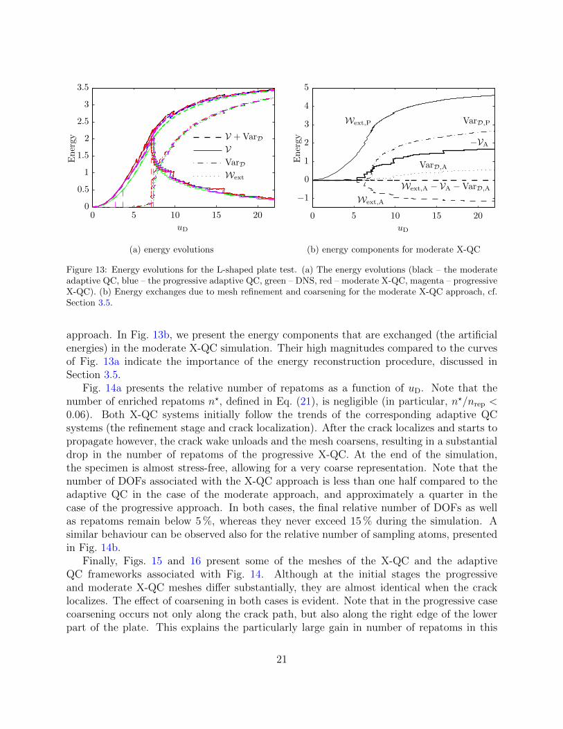
The energy evolutions appear in Fig. 13a as functions of uD. The energy balance (E)is clearly satisfied along the entire loading path, i.e. the thin dotted lines presenting thework performed by external forces Wext lie on top of the thick dashed lines representing V +VarD. Second, similarly to the reaction forces, we notice that the energy paths are almostindistinguishable from those of adaptive QC, demonstrating good accuracy of the X-QC

20

Wext

VarD

VV +VarD

Energy

uD

0 5 10 15 200

0.5

1

1.5

2

2.5

3

3.5

(a) energy evolutions

Wext,P VarD,P

Wext,A − VA −VarD,A

Wext,A

VarD,A

−VA

Energy

uD

0 5 10 15 20

−1

0

1

2

3

4

5

(b) energy components for moderate X-QC

Figure 13: Energy evolutions for the L-shaped plate test. (a) The energy evolutions (black – the moderateadaptive QC, blue – the progressive adaptive QC, green – DNS, red – moderate X-QC, magenta – progressiveX-QC). (b) Energy exchanges due to mesh refinement and coarsening for the moderate X-QC approach, cf.Section 3.5.

approach. In Fig. 13b, we present the energy components that are exchanged (the artificialenergies) in the moderate X-QC simulation. Their high magnitudes compared to the curvesof Fig. 13a indicate the importance of the energy reconstruction procedure, discussed inSection 3.5.

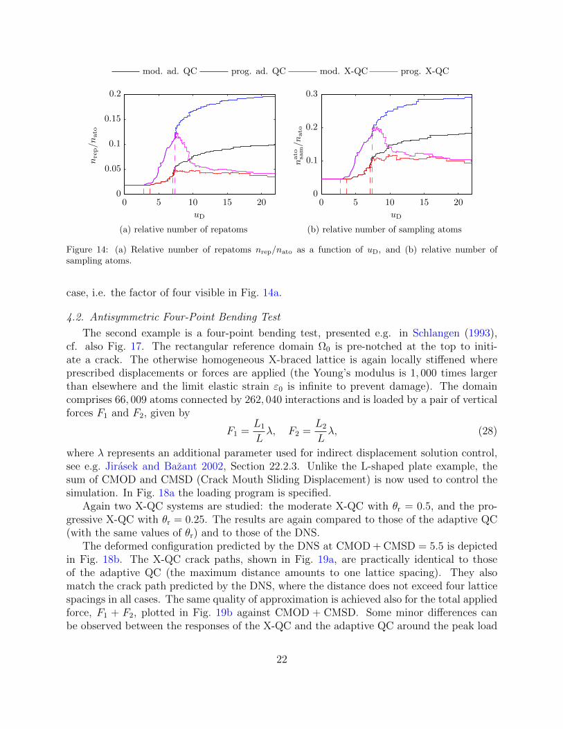
Fig. 14a presents the relative number of repatoms as a function of uD. Note that thenumber of enriched repatoms n?, defined in Eq. (21), is negligible (in particular, n?/nrep <0.06). Both X-QC systems initially follow the trends of the corresponding adaptive QCsystems (the refinement stage and crack localization). After the crack localizes and starts topropagate however, the crack wake unloads and the mesh coarsens, resulting in a substantialdrop in the number of repatoms of the progressive X-QC. At the end of the simulation,the specimen is almost stress-free, allowing for a very coarse representation. Note that thenumber of DOFs associated with the X-QC approach is less than one half compared to theadaptive QC in the case of the moderate approach, and approximately a quarter in thecase of the progressive approach. In both cases, the final relative number of DOFs as wellas repatoms remain below 5 %, whereas they never exceed 15 % during the simulation. Asimilar behaviour can be observed also for the relative number of sampling atoms, presentedin Fig. 14b.

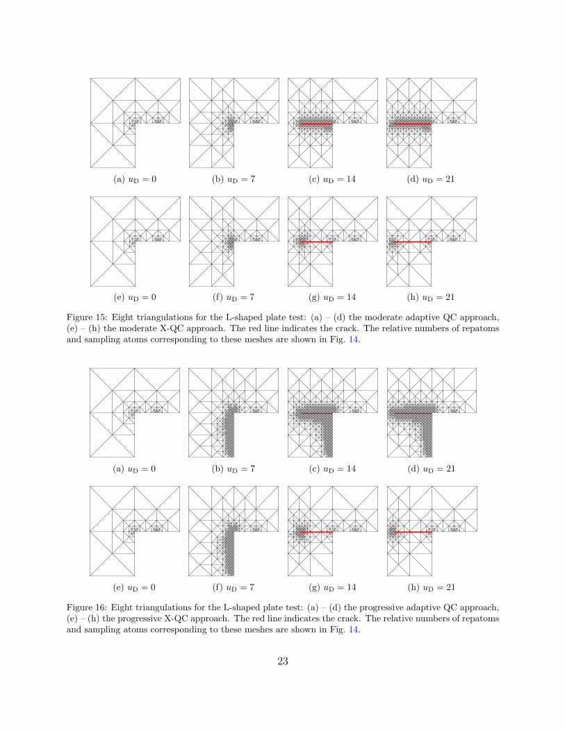
Finally, Figs. 15 and 16 present some of the meshes of the X-QC and the adaptiveQC frameworks associated with Fig. 14. Although at the initial stages the progressiveand moderate X-QC meshes differ substantially, they are almost identical when the cracklocalizes. The effect of coarsening in both cases is evident. Note that in the progressive casecoarsening occurs not only along the crack path, but also along the right edge of the lowerpart of the plate. This explains the particularly large gain in number of repatoms in this

21

prog. X-QCmod. X-QCprog. ad. QCmod. ad. QC

nrep/n

ato

uD

0 5 10 15 200

0.05

0.1

0.15

0.2

prog. X-QC

mod. X-QC

prog. ad. QC

mod. ad. QCnrep/n

ato

uD

0 5 10 15 200

0.05

0.1

0.15

0.2

(a) relative number of repatoms

nato

sam/n

ato

uD

0 5 10 15 200

0.1

0.2

0.3

(b) relative number of sampling atoms

Figure 14: (a) Relative number of repatoms nrep/nato as a function of uD, and (b) relative number ofsampling atoms.

case, i.e. the factor of four visible in Fig. 14a.

4.2. Antisymmetric Four-Point Bending Test

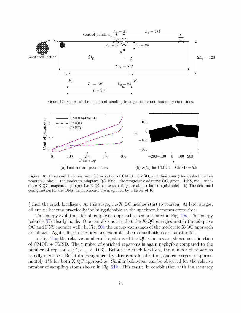
The second example is a four-point bending test, presented e.g. in Schlangen (1993),cf. also Fig. 17. The rectangular reference domain Ω0 is pre-notched at the top to initi-ate a crack. The otherwise homogeneous X-braced lattice is again locally stiffened whereprescribed displacements or forces are applied (the Young’s modulus is 1, 000 times largerthan elsewhere and the limit elastic strain ε0 is infinite to prevent damage). The domaincomprises 66, 009 atoms connected by 262, 040 interactions and is loaded by a pair of verticalforces F1 and F2, given by

F1 =L1

Lλ, F2 =

L2

Lλ, (28)

where λ represents an additional parameter used for indirect displacement solution control,see e.g. Jirasek and Bazant 2002, Section 22.2.3. Unlike the L-shaped plate example, thesum of CMOD and CMSD (Crack Mouth Sliding Displacement) is now used to control thesimulation. In Fig. 18a the loading program is specified.

Again two X-QC systems are studied: the moderate X-QC with θr = 0.5, and the pro-gressive X-QC with θr = 0.25. The results are again compared to those of the adaptive QC(with the same values of θr) and to those of the DNS.

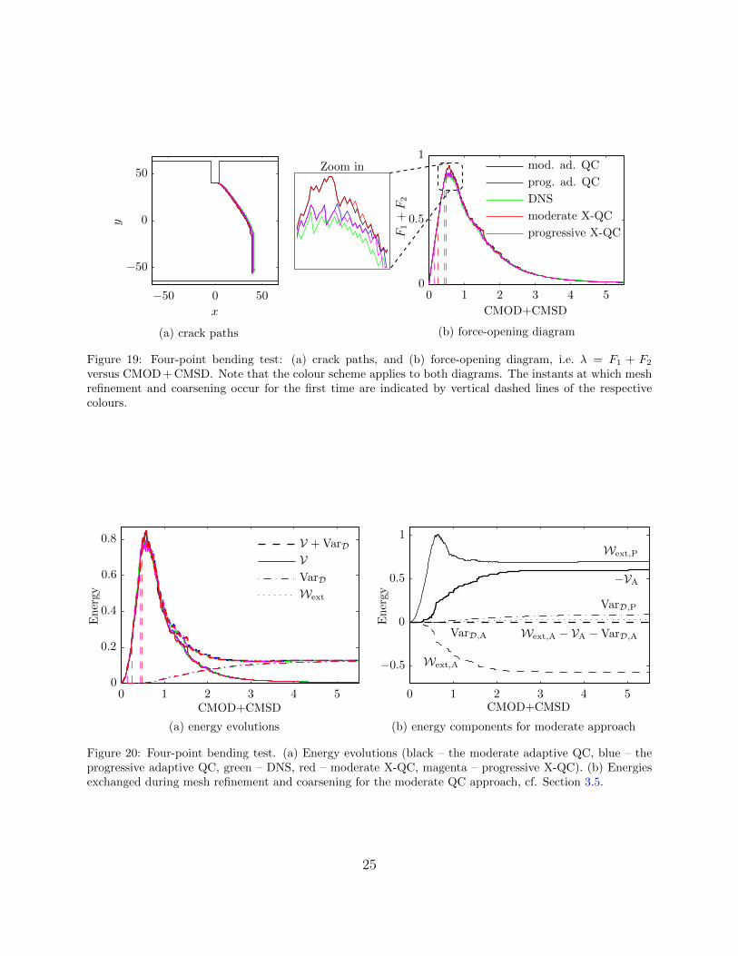
The deformed configuration predicted by the DNS at CMOD + CMSD = 5.5 is depictedin Fig. 18b. The X-QC crack paths, shown in Fig. 19a, are practically identical to thoseof the adaptive QC (the maximum distance amounts to one lattice spacing). They alsomatch the crack path predicted by the DNS, where the distance does not exceed four latticespacings in all cases. The same quality of approximation is achieved also for the total appliedforce, F1 + F2, plotted in Fig. 19b against CMOD + CMSD. Some minor differences canbe observed between the responses of the X-QC and the adaptive QC around the peak load

22

y

x

0 10 20 30 40 50 60 70

0

10

20

30

40

50

60

70

(a) uD = 0

y

x

0 10 20 30 40 50 60 70

0

10

20

30

40

50

60

70

(b) uD = 7

y

x

0 10 20 30 40 50 60 70

0

10

20

30

40

50

60

70

(c) uD = 14

y

x

0 10 20 30 40 50 60 70

0

10

20

30

40

50

60

70

(d) uD = 21

y

x

0 10 20 30 40 50 60 70

0

10

20

30

40

50

60

70

(e) uD = 0

y

x

0 10 20 30 40 50 60 70

0

10

20

30

40

50

60

70

(f) uD = 7

y

x

0 10 20 30 40 50 60 70

0

10

20

30

40

50

60

70

(g) uD = 14

y

x

0 10 20 30 40 50 60 70

0

10

20

30

40

50

60

70

(h) uD = 21

Figure 15: Eight triangulations for the L-shaped plate test: (a) – (d) the moderate adaptive QC approach,(e) – (h) the moderate X-QC approach. The red line indicates the crack. The relative numbers of repatomsand sampling atoms corresponding to these meshes are shown in Fig. 14.

y

x

0 10 20 30 40 50 60 70

0

10

20

30

40

50

60

70

(a) uD = 0

y

x

0 10 20 30 40 50 60 70

0

10

20

30

40

50

60

70

(b) uD = 7

y

x

0 10 20 30 40 50 60 70

0

10

20

30

40

50

60

70

(c) uD = 14

y

x

0 10 20 30 40 50 60 70

0

10

20

30

40

50

60

70

(d) uD = 21

y

x

0 10 20 30 40 50 60 70

0

10

20

30

40

50

60

70

(e) uD = 0

y

x

0 10 20 30 40 50 60 70

0

10

20

30

40

50

60

70

(f) uD = 7

y

x

0 10 20 30 40 50 60 70

0

10

20

30

40

50

60

70

(g) uD = 14

y

x

0 10 20 30 40 50 60 70

0

10

20

30

40

50

60

70

(h) uD = 21

Figure 16: Eight triangulations for the L-shaped plate test: (a) – (d) the progressive adaptive QC approach,(e) – (h) the progressive X-QC approach. The red line indicates the crack. The relative numbers of repatomsand sampling atoms corresponding to these meshes are shown in Fig. 14.

23

X-braced lattice

control points

2Lx = 512

L = 256

L2 = 24L1 = 232

L2 = 24 L1 = 232

ay = 24ax = 8

2Ly = 128

y

x

F1F2

Ω0

Figure 17: Sketch of the four-point bending test: geometry and boundary conditions.

CMSDCMODCMOD+CMSD

Con

trol

param

eter

Time step0 100 200 300 400

0

2

4

(a) load control parameters

y

x

−200−100 0 100 200

−200

−100

0

100

(b) r(tk) for CMOD + CMSD = 5.5

Figure 18: Four-point bending test: (a) evolution of CMOD, CMSD, and their sum (the applied loadingprogram); black – the moderate adaptive QC, blue – the progressive adaptive QC, green – DNS, red – mod-erate X-QC, magenta – progressive X-QC (note that they are almost indistinguishable). (b) The deformedconfiguration for the DNS; displacements are magnified by a factor of 10.

(when the crack localizes). At this stage, the X-QC meshes start to coarsen. At later stages,all curves become practically indistinguishable as the specimen becomes stress-free.

The energy evolutions for all employed approaches are presented in Fig. 20a. The energybalance (E) clearly holds. One can also notice that the X-QC energies match the adaptiveQC and DNS energies well. In Fig. 20b the energy exchanges of the moderate X-QC approachare shown. Again, like in the previous example, their contributions are substantial.

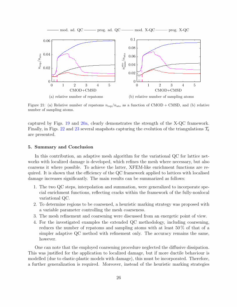
In Fig. 21a, the relative number of repatoms of the QC schemes are shown as a functionof CMOD + CMSD. The number of enriched repatoms is again negligible compared to thenumber of repatoms (n?/nrep < 0.03). Before the crack localizes, the number of repatomsrapidly increases. But it drops significantly after crack localization, and converges to approx-imately 1 % for both X-QC approaches. Similar behaviour can be observed for the relativenumber of sampling atoms shown in Fig. 21b. This result, in combination with the accuracy

24

y

x

−50 0 50

−50

0

50

(a) crack paths

progressive X-QC

moderate X-QC

DNS

prog. ad. QC

mod. ad. QC

F1+F2

CMOD+CMSD

0 1 2 3 4 50

0.5

1

(b) force-opening diagram

0.5 0.6 0.7 0.8 0.9

0.65

0.7

0.75

0.8

0.85

0.9

0.95Zoom in

Figure 19: Four-point bending test: (a) crack paths, and (b) force-opening diagram, i.e. λ = F1 + F2

versus CMOD + CMSD. Note that the colour scheme applies to both diagrams. The instants at which meshrefinement and coarsening occur for the first time are indicated by vertical dashed lines of the respectivecolours.

Wext

VarD

VV +VarD

Energy

CMOD+CMSD0 1 2 3 4 5

0

0.2

0.4

0.6

0.8

(a) energy evolutions

Wext,A

Wext,A − VA −VarD,AVarD,A

VarD,P

−VA

Wext,P

Energy

CMOD+CMSD0 1 2 3 4 5

−0.5

0

0.5

1

(b) energy components for moderate approach

Figure 20: Four-point bending test. (a) Energy evolutions (black – the moderate adaptive QC, blue – theprogressive adaptive QC, green – DNS, red – moderate X-QC, magenta – progressive X-QC). (b) Energiesexchanged during mesh refinement and coarsening for the moderate QC approach, cf. Section 3.5.

25

prog. X-QCmod. X-QCprog. ad. QCmod. ad. QC

nrep/n

ato

uD

0 5 10 15 200

0.05

0.1

0.15

0.2

prog. X-QC

mod. X-QC

prog. ad. QC

mod. ad. QCnrep/n

ato

CMOD+CMSD

0 1 2 3 4 50

0.02

0.04

0.06

(a) relative number of repatoms

nato

sam/n

ato

CMOD+CMSD

0 1 2 3 4 50

0.02

0.04

0.06

0.08

0.1

(b) relative number of sampling atoms

Figure 21: (a) Relative number of repatoms nrep/nato as a function of CMOD + CMSD, and (b) relativenumber of sampling atoms.

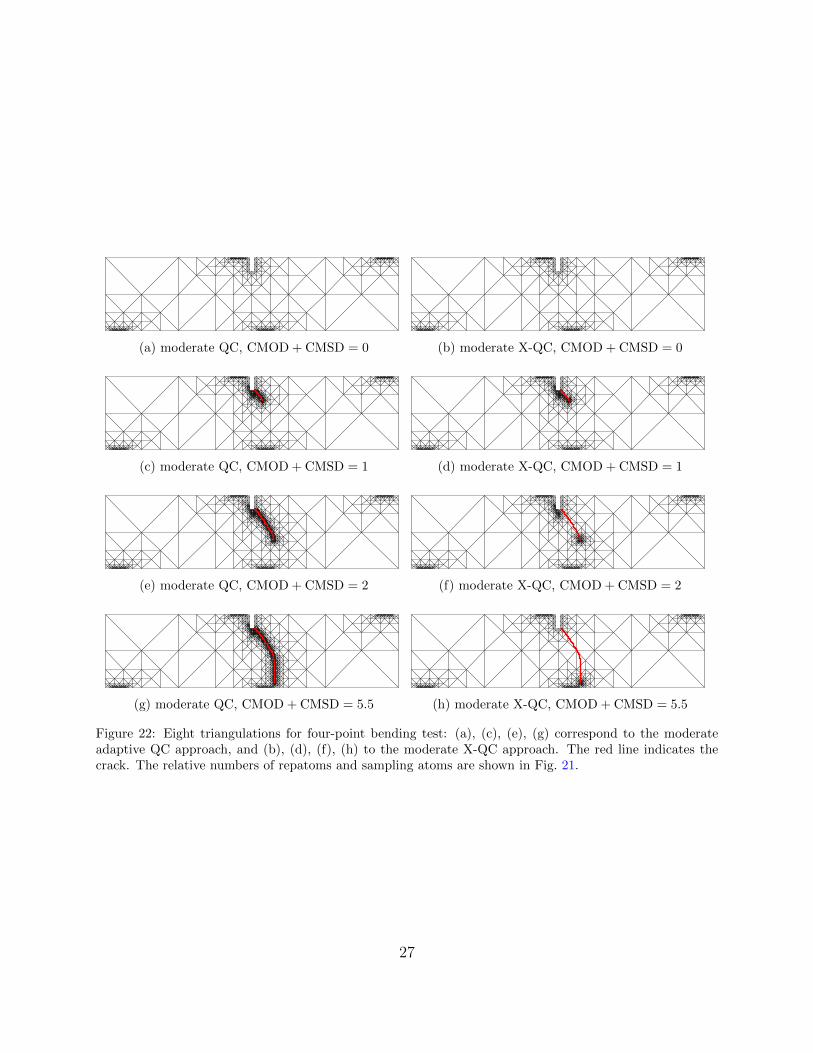
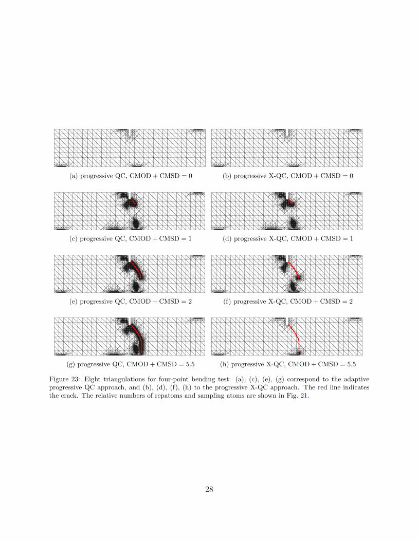
captured by Figs. 19 and 20a, clearly demonstrates the strength of the X-QC framework.Finally, in Figs. 22 and 23 several snapshots capturing the evolution of the triangulations Tkare presented.

5. Summary and Conclusion

In this contribution, an adaptive mesh algorithm for the variational QC for lattice net-works with localized damage is developed, which refines the mesh where necessary, but alsocoarsens it where possible. To achieve the latter, XFEM-like enrichment functions are re-quired. It is shown that the efficiency of the QC framework applied to lattices with localiseddamage increases significantly. The main results can be summarized as follows:

1. The two QC steps, interpolation and summation, were generalized to incorporate spe-cial enrichment functions, reflecting cracks within the framework of the fully-nonlocalvariational QC.

2. To determine regions to be coarsened, a heuristic marking strategy was proposed witha variable parameter controlling the mesh coarseness.

3. The mesh refinement and coarsening were discussed from an energetic point of view.

4. For the investigated examples the extended QC methodology, including coarsening,reduces the number of repatoms and sampling atoms with at least 50 % of that of asimpler adaptive QC method with refinement only. The accuracy remains the same,however.

One can note that the employed coarsening procedure neglected the diffusive dissipation.This was justified for the application to localized damage, but if more ductile behaviour ismodelled (due to elastic-plastic models with damage), this must be incorporated. Therefore,a further generalization is required. Moreover, instead of the heuristic marking strategies

26

y

x

−250 −200 −150 −100 −50 0 50 100 150 200 250

−200

−150

−100

−50

0

50

100

150

200

(a) moderate QC, CMOD + CMSD = 0

y

x

−250 −200 −150 −100 −50 0 50 100 150 200 250

−200

−150

−100

−50

0

50

100

150

200

(b) moderate X-QC, CMOD + CMSD = 0

y

x

−250 −200 −150 −100 −50 0 50 100 150 200 250

−200

−150

−100

−50

0

50

100

150

200

(c) moderate QC, CMOD + CMSD = 1

y

x

−250 −200 −150 −100 −50 0 50 100 150 200 250

−200

−150

−100

−50

0

50

100

150

200

(d) moderate X-QC, CMOD + CMSD = 1

y

x

−250 −200 −150 −100 −50 0 50 100 150 200 250

−200

−150

−100

−50

0

50

100

150

200

(e) moderate QC, CMOD + CMSD = 2

y

x

−250 −200 −150 −100 −50 0 50 100 150 200 250

−200

−150

−100

−50

0

50

100

150

200

(f) moderate X-QC, CMOD + CMSD = 2

y

x

−250 −200 −150 −100 −50 0 50 100 150 200 250

−200

−150

−100

−50

0

50

100

150

200

(g) moderate QC, CMOD + CMSD = 5.5

y

x

−250 −200 −150 −100 −50 0 50 100 150 200 250

−200

−150

−100

−50

0

50

100

150

200

(h) moderate X-QC, CMOD + CMSD = 5.5

Figure 22: Eight triangulations for four-point bending test: (a), (c), (e), (g) correspond to the moderateadaptive QC approach, and (b), (d), (f), (h) to the moderate X-QC approach. The red line indicates thecrack. The relative numbers of repatoms and sampling atoms are shown in Fig. 21.

27

y

x

−250 −200 −150 −100 −50 0 50 100 150 200 250

−200

−150

−100

−50

0

50

100

150

200

(a) progressive QC, CMOD + CMSD = 0

y

x

−250 −200 −150 −100 −50 0 50 100 150 200 250

−200

−150

−100

−50

0

50

100

150

200

(b) progressive X-QC, CMOD + CMSD = 0

y

x

−250 −200 −150 −100 −50 0 50 100 150 200 250

−200

−150

−100

−50

0

50

100

150

200

(c) progressive QC, CMOD + CMSD = 1

y

x

−250 −200 −150 −100 −50 0 50 100 150 200 250

−200

−150

−100

−50

0

50

100

150

200

(d) progressive X-QC, CMOD + CMSD = 1

y

x

−250 −200 −150 −100 −50 0 50 100 150 200 250

−200

−150

−100

−50

0

50

100

150

200

(e) progressive QC, CMOD + CMSD = 2

y

x

−250 −200 −150 −100 −50 0 50 100 150 200 250

−200

−150

−100

−50

0

50

100

150

200

(f) progressive X-QC, CMOD + CMSD = 2

y

x

−250 −200 −150 −100 −50 0 50 100 150 200 250

−200

−150

−100

−50

0

50

100

150

200

(g) progressive QC, CMOD + CMSD = 5.5

y

x

−250 −200 −150 −100 −50 0 50 100 150 200 250

−200

−150

−100

−50

0

50

100

150

200

(h) progressive X-QC, CMOD + CMSD = 5.5

Figure 23: Eight triangulations for four-point bending test: (a), (c), (e), (g) correspond to the adaptiveprogressive QC approach, and (b), (d), (f), (h) to the progressive X-QC approach. The red line indicatesthe crack. The relative numbers of repatoms and sampling atoms are shown in Fig. 21.

28

used here, goal-oriented error estimators may be used to further improve the accuracy andefficiency of the QC methodology. The variational foundation of the method provides anideal platform for this, cf. e.g. Radovitzky and Ortiz (1999). The same X-QC frameworkcan also be employed for the description of heterogeneities in otherwise homogeneous latticenetworks. These aspects are, however, outside the scope of this contribution and will bereported separately.

Acknowledgements

This work was supported by the Czech Science Foundation (GACR), through projectNo. 14-00420S. In addition, JZ acknowledges a partial support by the Czech Science Foun-dation, through project No. 16-34894L.

References

Agathos, K., Chatzi, E., Bordas, S.P., 2016a. Stable 3D extended finite elements with higherorder enrichment for accurate non planar fracture. Computer Methods in Applied Me-chanics and Engineering 306, 19 – 46. URL: http://www.sciencedirect.com/science/article/pii/S0045782516301050, doi: http://dx.doi.org/10.1016/j.cma.2016.03.

023.

Agathos, K., Chatzi, E., Bordas, S.P.A., Talaslidis, D., 2016b. A well-conditioned and opti-mally convergent XFEM for 3D linear elastic fracture. International Journal for NumericalMethods in Engineering 105, 643–677. URL: http://dx.doi.org/10.1002/nme.4982,doi: 10.1002/nme.4982. nme.4982.

Amelang, J.S., Venturini, G.N., Kochmann, D.M., 2015. Summation rules for a fullynonlocal energy-based quasicontinuum method. Journal of the Mechanics and Physicsof Solids 82, 378–413. URL: http://www.sciencedirect.com/science/article/pii/S0022509615000630, doi: http://dx.doi.org/10.1016/j.jmps.2015.03.007.

Aubertin, P., Rethore, J., de Borst, R., 2009. Energy conservation of atomistic/continuumcoupling. International Journal for Numerical Methods in Engineering 78, 1365–1386.URL: http://dx.doi.org/10.1002/nme.2542, doi: 10.1002/nme.2542.

Aubertin, P., Rethore, J., de Borst, R., 2010. A coupled molecular dynamics and extendedfinite element method for dynamic crack propagation. International Journal for NumericalMethods in Engineering 81, 72–88. URL: http://dx.doi.org/10.1002/nme.2675, doi:10.1002/nme.2675.

Babuska, I., Banerjee, U., 2012. Stable generalized finite element method (SGFEM). Com-puter Methods in Applied Mechanics and Engineering 201204, 91 – 111. URL: http:

//www.sciencedirect.com/science/article/pii/S0045782511003082, doi: http://

dx.doi.org/10.1016/j.cma.2011.09.012.

29

Babuska, I., Melenk, J.M., 1997. The partition of unity method. International Jour-nal for Numerical Methods in Engineering 40, 727–758. URL: http://dx.doi.org/10.1002/(SICI)1097-0207(19970228)40:4<727::AID-NME86>3.0.CO;2-N, doi: 10.1002/

(SICI)1097-0207(19970228)40:4<727::AID-NME86>3.0.CO;2-N.

Becker, R., Rannacher, R., 2001. An optimal control approach to a posteriori error estimationin finite element methods. Acta Numerica 10, 1–102. URL: http://journals.cambridge.org/article_S0962492901000010, doi: 10.1017/S0962492901000010.

Beex, L.A.A., Kerfriden, P., Rabczuk, T., Bordas, S.P.A., 2014a. Quasicontinuum-based multiscale approaches for plate-like beam lattices experiencing in-plane andout-of-plane deformation. Computer Methods in Applied Mechanics and Engineer-ing 279, 348–378. URL: http://www.sciencedirect.com/science/article/pii/

S0045782514002047, doi: http://dx.doi.org/10.1016/j.cma.2014.06.018.

Beex, L.A.A., Peerlings, R.H.J., Geers, M.G.D., 2011. A quasicontinuum methodology formultiscale analyses of discrete microstructural models. International Journal for NumericalMethods in Engineering 87, 701–718. URL: http://dx.doi.org/10.1002/nme.3134, doi:10.1002/nme.3134.

Beex, L.A.A., Peerlings, R.H.J., Geers, M.G.D., 2014b. Central summation in the quasicon-tinuum method. Journal of the Mechanics and Physics of Solids 70, 242–261. URL: http://www.sciencedirect.com/science/article/pii/S0022509614001100, doi: http://

dx.doi.org/10.1016/j.jmps.2014.05.019.

Beex, L.A.A., Peerlings, R.H.J., Geers, M.G.D., 2014c. A multiscale quasicontinuum methodfor dissipative lattice models and discrete networks. Journal of the Mechanics and Physicsof Solids 64, 154–169. URL: http://www.sciencedirect.com/science/article/pii/S0022509613002445, doi: http://dx.doi.org/10.1016/j.jmps.2013.11.010.

Beex, L.A.A., Peerlings, R.H.J., Geers, M.G.D., 2014d. A multiscale quasicontinuum methodfor lattice models with bond failure and fiber sliding. Computer Methods in Applied Me-chanics and Engineering 269, 108–122. URL: http://www.sciencedirect.com/science/article/pii/S004578251300279X, doi: http://dx.doi.org/10.1016/j.cma.2013.10.

027.

Beex, L.A.A., Peerlings, R.H.J., van Os, K., Geers, M.G.D., 2015a. The mechanical relia-bility of an electronic textile investigated using the virtual-power-based quasicontinuummethod. Mechanics of Materials 80, Part A, 52–66. URL: http://www.sciencedirect.com/science/article/pii/S0167663614001495, doi: http://dx.doi.org/10.1016/j.

mechmat.2014.08.001.

Beex, L.A.A., Rokos, O., Zeman, J., Bordas, S.P.A., 2015b. Higher-order quasicontinuummethods for elastic and dissipative lattice models: uniaxial deformation and pure bending.GAMM-Mitteilungen 38, 344–368. URL: http://dx.doi.org/10.1002/gamm.201510018,doi: 10.1002/gamm.201510018.

30

Beex, L.A.A., Verberne, C.W., Peerlings, R.H.J., 2013. Experimental identification of a lat-tice model for woven fabrics: Application to electronic textile. Composites Part A: AppliedScience and Manufacturing 48, 82–92. URL: http://www.sciencedirect.com/science/article/pii/S1359835X13000134, doi: http://dx.doi.org/10.1016/j.compositesa.

2012.12.014.

Belytschko, T., Black, T., 1999. Elastic crack growth in finite elements withminimal remeshing. International Journal for Numerical Methods in Engineer-ing 45, 601–620. URL: http://dx.doi.org/10.1002/(SICI)1097-0207(19990620)

45:5<601::AID-NME598>3.0.CO;2-S, doi: 10.1002/(SICI)1097-0207(19990620)45:

5<601::AID-NME598>3.0.CO;2-S.

Belytschko, T., Moes, N., Usui, S., Parimi, C., 2001. Arbitrary discontinuities in finiteelements. International Journal for Numerical Methods in Engineering 50, 993–1013.URL: http://dx.doi.org/10.1002/1097-0207(20010210)50:4<993::AID-NME164>3.

0.CO;2-M, doi: 10.1002/1097-0207(20010210)50:4<993::AID-NME164>3.0.CO;2-M.

Bosco, E., Peerlings, R., Geers, M., 2015a. Explaining irreversible hygroscopic strains in pa-per: a multi-scale modelling study on the role of fibre activation and micro-compressions.Mechanics of Materials 91, Part 1, 76 – 94. URL: http://www.sciencedirect.

com/science/article/pii/S016766361500157X, doi: http://dx.doi.org/10.1016/j.

mechmat.2015.07.009.

Bosco, E., Peerlings, R.H., Geers, M.G., 2015b. Predicting hygro-elastic properties of pa-per sheets based on an idealized model of the underlying fibrous network. InternationalJournal of Solids and Structures 5657, 43 – 52. URL: http://www.sciencedirect.

com/science/article/pii/S0020768314004600, doi: http://dx.doi.org/10.1016/j.

ijsolstr.2014.12.006.

Bourdin, B., 2007. Numerical implementation of the variational formulation for quasi-staticbrittle fracture. Interfaces and Free Boundaries 9, 411–430. doi: 10.4171/IFB/171.

Bourdin, B., Francfort, G.A., Marigo, J.J., 2000. Numerical experiments in revisited brittlefracture. Journal of the Mechanics and Physics of Solids 48, 797–826. URL: http://www.sciencedirect.com/science/article/pii/S0022509699000289, doi: http://dx.doi.

org/10.1016/S0022-5096(99)00028-9.

Bourdin, B., Francfort, G.A., Marigo, J.J., 2008. The Variational Approach to Fracture.Springer Netherlands. URL: http://www.springer.com/gp/book/9781402063947.

Burke, S., Ortner, C., Sli, E., 2010. An Adaptive Finite Element Approximation of a Varia-tional Model of Brittle Fracture. SIAM Journal on Numerical Analysis 48, 980–1012. URL:http://epubs.siam.org/doi/abs/10.1137/080741033, doi: 10.1137/080741033.

Chen, L., Zhang, C.S., 2010. A coarsening algorithm on adaptive grids by newest vertexbisection and its applications. J. Comp. Math. 28, 767–789.

31

Curtin, W.A., Miller, R.E., 2003. Atomistic/continuum coupling in computational materialsscience. Modelling and Simulation in Materials Science and Engineering 11, R33. URL:http://stacks.iop.org/0965-0393/11/i=3/a=201.

Cusatis, G., Bazant, Z.P., Cedolin, L., 2006. Confinement-shear lattice CSL model forfracture propagation in concrete. Computer Methods in Applied Mechanics and Engi-neering 195, 7154–7171. URL: http://www.sciencedirect.com/science/article/pii/S0045782505003956, doi: http://dx.doi.org/10.1016/j.cma.2005.04.019.

Daux, C., Moes, N., Dolbow, J., Sukumar, N., Belytschko, T., 2000. Arbitrary branchedand intersecting cracks with the extended finite element method. International Jour-nal for Numerical Methods in Engineering 48, 1741–1760. URL: http://dx.doi.org/10.1002/1097-0207(20000830)48:12<1741::AID-NME956>3.0.CO;2-L, doi: 10.1002/

1097-0207(20000830)48:12<1741::AID-NME956>3.0.CO;2-L.

Elias, J., Vorechovsky, M., Skocek, J., Bazant, Z.P., 2015. Stochastic discrete meso-scalesimulations of concrete fracture: Comparison to experimental data. Engineering FractureMechanics 135, 1–16. URL: http://www.sciencedirect.com/science/article/pii/

S0013794415000053, doi: http://dx.doi.org/10.1016/j.engfracmech.2015.01.004.

Fries, T.P., 2008. A corrected XFEM approximation without problems in blending elements.International Journal for Numerical Methods in Engineering 75, 503–532. URL: http://dx.doi.org/10.1002/nme.2259, doi: 10.1002/nme.2259.

Fries, T.P., Baydoun, M., 2012. Crack propagation with the extended finite element methodand a hybrid explicit–implicit crack description. International Journal for Numerical Meth-ods in Engineering 89, 1527–1558. URL: http://dx.doi.org/10.1002/nme.3299, doi:10.1002/nme.3299.

Fries, T.P., Belytschko, T., 2010. The extended/generalized finite element method: Anoverview of the method and its applications. International Journal for Numerical Methodsin Engineering 84, 253–304. URL: http://dx.doi.org/10.1002/nme.2914, doi: 10.

1002/nme.2914.

Funken, S., Praetorius, D., Wissgott, P., 2010. Efficient implementation of adaptive P1-FEMin Matlab. Comput. Methods Appl. Math. 11, 460–490. doi: 10.2478/cmam-2011-0026.

Gracie, R., Belytschko, T., 2009. Concurrently coupled atomistic and XFEM models fordislocations and cracks. International Journal for Numerical Methods in Engineering 78,354–378. URL: http://dx.doi.org/10.1002/nme.2488, doi: 10.1002/nme.2488.

Grassl, P., Jirasek, M., 2010. Meso-scale approach to modelling the fracture processzone of concrete subjected to uniaxial tension. International Journal of Solids andStructures 47, 957–968. URL: http://www.sciencedirect.com/science/article/pii/S0020768309004752, doi: http://dx.doi.org/10.1016/j.ijsolstr.2009.12.010.

32

Han, W., Reddy, B.D., 1995. Computational plasticity: The variational basis and numericalanalysis. Computational Mechanics Advances 2, 283–400.

Hofacker, M., Miehe, C., 2012. Continuum phase field modeling of dynamic fracture: vari-ational principles and staggered FE implementation. International Journal of Fracture178, 113–129. URL: http://dx.doi.org/10.1007/s10704-012-9753-8, doi: 10.1007/

s10704-012-9753-8.

Iyer, M., Gavini, V., 2011. A field theoretical approach to the quasi-continuum method.Journal of the Mechanics and Physics of Solids 59, 1506–1535. URL: http://www.

sciencedirect.com/science/article/pii/S0022509610002425, doi: http://dx.doi.

org/10.1016/j.jmps.2010.12.002.

Jirasek, M., Bazant, Z.P., 2002. Inelastic Analysis of Structures. John Wiley & Sons. URL:https://books.google.nl/books?id=8mz-xPdvH00C.

Jirasek, M., Zeman, J., 2015. Localization study of a regularized variational damagemodel. International Journal of Solids and Structures 6970, 131–151. URL: http:

//www.sciencedirect.com/science/article/pii/S0020768315002620, doi: http://

dx.doi.org/10.1016/j.ijsolstr.2015.06.001.

Kulachenko, A., Uesaka, T., 2012. Direct simulations of fiber network deformationand failure. Mechanics of Materials 51, 1–14. URL: http://www.sciencedirect.

com/science/article/pii/S0167663612000683, doi: http://dx.doi.org/10.1016/j.

mechmat.2012.03.010.

Laborde, P., Pommier, J., Renard, Y., Salan, M., 2005. High-order extended finite elementmethod for cracked domains. International Journal for Numerical Methods in Engineering64, 354–381. URL: http://dx.doi.org/10.1002/nme.1370, doi: 10.1002/nme.1370.

Liu, J.X., Chen, Z.T., Li, K.C., 2010. A 2-D lattice model for simulating the fail-ure of paper. Theoretical and Applied Fracture Mechanics 54, 1–10. URL: http:

//www.sciencedirect.com/science/article/pii/S016784421000039X, doi: http://

dx.doi.org/10.1016/j.tafmec.2010.06.009.

Luskin, M., Ortner, C., 2013. Atomistic-to-continuum coupling. Acta Numerica 22, 397–508. URL: http://journals.cambridge.org/article_S0962492913000068, doi: 10.

1017/S0962492913000068.

Melenk, J., Babuska, I., 1996. The partition of unity finite element method: Ba-sic theory and applications. Computer Methods in Applied Mechanics and Engineer-ing 139, 289 – 314. URL: http://www.sciencedirect.com/science/article/pii/

S0045782596010870, doi: http://dx.doi.org/10.1016/S0045-7825(96)01087-0.

Memarnahavandi, A., Larsson, F., Runesson, K., 2015. A goal-oriented adaptive procedurefor the quasi-continuum method with cluster approximation. Computational Mechanics

33

55, 617–642. URL: http://dx.doi.org/10.1007/s00466-015-1127-4, doi: 10.1007/

s00466-015-1127-4.

Mesgarnejad, A., Bourdin, B., Khonsari, M.M., 2015. Validation simulations for thevariational approach to fracture. Computer Methods in Applied Mechanics and Engi-neering 290, 420–437. URL: http://www.sciencedirect.com/science/article/pii/S004578251400423X, doi: http://dx.doi.org/10.1016/j.cma.2014.10.052.

Mielke, A., 2003. Energetic formulation of multiplicative elasto-plasticity using dissipationdistances. Continuum Mechanics and Thermodynamics 15, 351–382. URL: http://dx.doi.org/10.1007/s00161-003-0120-x, doi: 10.1007/s00161-003-0120-x.

Mielke, A., Roubıcek, T., 2015. Rate-Independent Systems: Theory and Application. 1 ed.,Springer-Verlag New York. URL: http://www.springer.com/us/book/9781493927050,doi: 10.1007/978-1-4939-2706-7.

Mielke, A., Theil, F., Levitas, V.I., 2002. A variational formulation of rate-independentphase transformations using an extremum principle. Archive for Rational Mechanics andAnalysis 162, 137–177. URL: http://dx.doi.org/10.1007/s002050200194, doi: 10.

1007/s002050200194.

Miller, R.E., Tadmor, E.B., 2002. The quasicontinuum method: Overview, applicationsand current directions. Journal of Computer-Aided Materials Design 9, 203–239. URL:http://dx.doi.org/10.1023/A%3A1026098010127, doi: 10.1023/A:1026098010127.

Miller, R.E., Tadmor, E.B., 2009. A unified framework and performance benchmark of four-teen multiscale atomistic/continuum coupling methods. Modelling and Simulation in Ma-terials Science and Engineering 17, 053001. URL: http://stacks.iop.org/0965-0393/17/i=5/a=053001.

Moes, N., Dolbow, J., Belytschko, T., 1999. A finite element method for crackgrowth without remeshing. International Journal for Numerical Methods in Engi-neering 46, 131–150. URL: http://dx.doi.org/10.1002/(SICI)1097-0207(19990910)46:1<131::AID-NME726>3.0.CO;2-J, doi: 10.1002/(SICI)1097-0207(19990910)46:

1<131::AID-NME726>3.0.CO;2-J.

Muhlhaus, H.B., Aifantis, E.C., 1991. A variational principle for gradient plastic-ity. International Journal of Solids and Structures 28, 845–857. URL: http://www.

sciencedirect.com/science/article/pii/002076839190004Y, doi: http://dx.doi.

org/10.1016/0020-7683(91)90004-Y.

Oden, J., Prudhomme, S., 2002. Estimation of modeling error in computational mechanics.Journal of Computational Physics 182, 496–515. URL: http://www.sciencedirect.com/science/article/pii/S0021999102971834, doi: http://dx.doi.org/10.1006/jcph.

2002.7183.

34

Peng, X., Cao, J., 2005. A continuum mechanics-based non-orthogonal constitutivemodel for woven composite fabrics. Composites Part A: Applied Science and Manufac-turing 36, 859 – 874. URL: http://www.sciencedirect.com/science/article/pii/

S1359835X04002593, doi: http://dx.doi.org/10.1016/j.compositesa.2004.08.008.

Pham, K., Marigo, J.J., Maurini, C., 2011. The issues of the uniqueness and the stabilityof the homogeneous response in uniaxial tests with gradient damage models. Journal ofthe Mechanics and Physics of Solids 59, 1163–1190. URL: http://www.sciencedirect.com/science/article/pii/S002250961100055X, doi: http://dx.doi.org/10.1016/j.

jmps.2011.03.010.

Prudhomme, S., Bauman, P.T., Oden, J.T., 2006. Error control for molecular statics prob-lems. International Journal for Multiscale Computational Engineering 4, 647–662. doi:10.1615/IntJMultCompEng.v4.i5-6.60.

Radovitzky, R., Ortiz, M., 1999. Error estimation and adaptive meshing in stronglynonlinear dynamic problems. Computer Methods in Applied Mechanics and Engineer-ing 172, 203 – 240. URL: http://www.sciencedirect.com/science/article/pii/

S0045782598002308, doi: http://dx.doi.org/10.1016/S0045-7825(98)00230-8.

Ridruejo, A., Gonzalez, C., LLorca, J., 2010. Damage micromechanisms and notch sensi-tivity of glass-fiber non-woven felts: An experimental and numerical study. Journal ofthe Mechanics and Physics of Solids 58, 1628–1645. URL: http://www.sciencedirect.com/science/article/pii/S0022509610001341, doi: http://dx.doi.org/10.1016/j.

jmps.2010.07.005.

Rivara, M.C., 1997. New longest-edge algorithms for the refinement and/or improvement ofunstructured triangulations. International Journal for Numerical Methods in Engineering40, 3313–3324. doi: 10.1002/(SICI)1097-0207(19970930)40:18<3313::AID-NME214>

3.0.CO;2-\#.

Rokos, O., Beex, L.A.A., Zeman, J., Peerlings, R.H.J., 2016. A variational formula-tion of dissipative quasicontinuum methods. International Journal of Solids and Struc-tures 102103, 214 – 229. URL: //www.sciencedirect.com/science/article/pii/

S0020768316302943, doi: http://dx.doi.org/10.1016/j.ijsolstr.2016.10.003.

Rokos, O., Peerlings, R.H.J., Zeman, J., Beex, L.A.A., 2017. An adaptive variational qua-sicontinuum methodology for lattice networks with localized damage. International Jour-nal for Numerical Methods in Engineering , n/a–n/aURL: http://dx.doi.org/10.1002/nme.5518, doi: 10.1002/nme.5518. nme.5518.

Schlangen, E., 1993. Experimental and Numerical Analysis of Fracture Processes in Concrete.Ph.D. thesis. Technische Universiteit Delft. TU Delft, 2600 AA Delft, The Netherlands.

35

Schlangen, E., van Mier, J.G.M., 1992. Experimental and numerical analysis of mi-cromechanisms of fracture of cement-based composites. Cement and Concrete Com-posites 14, 105–118. URL: http://www.sciencedirect.com/science/article/pii/

095894659290004F, doi: http://dx.doi.org/10.1016/0958-9465(92)90004-F.

Strouboulis, T., Babuska, I., Copps, K., 2000a. The design and analysis of the gen-eralized finite element method. Computer Methods in Applied Mechanics and Engi-neering 181, 43 – 69. URL: http://www.sciencedirect.com/science/article/pii/

S0045782599000729, doi: http://dx.doi.org/10.1016/S0045-7825(99)00072-9.

Strouboulis, T., Copps, K., Babuska, I., 2000b. The generalized finite element method:an example of its implementation and illustration of its performance. InternationalJournal for Numerical Methods in Engineering 47, 1401–1417. URL: http://dx.doi.

org/10.1002/(SICI)1097-0207(20000320)47:8<1401::AID-NME835>3.0.CO;2-8, doi:10.1002/(SICI)1097-0207(20000320)47:8<1401::AID-NME835>3.0.CO;2-8.

Tadmor, E.B., Miller, R.E., 2011. Modeling Materials: Continuum, Atomistic and MultiscaleTechniques. Cambridge University Press. URL: http://books.google.cz/books?id=5PLvc6tdsjcC.

Tadmor, E.B., Ortiz, M., Phillips, R., 1996. Quasicontinuum analysis of de-fects in solids. Philosophical Magazine A 73, 1529–1563. URL: http:

//dx.doi.org/10.1080/01418619608243000, doi: 10.1080/01418619608243000,arXiv:http://dx.doi.org/10.1080/01418619608243000.

Talebi, H., Silani, M., Bordas, S., Kerfriden, P., Rabczuk, T., 2013. Molecular dynam-ics/XFEM coupling by a three-dimensional extended bridging domain with applicationsto dynamic brittle fracture. International Journal for Multiscale Computational Engineer-ing 11, 527–541. doi: 10.1615/IntJMultCompEng.2013005838.

Ventura, G., Gracie, R., Belytschko, T., 2009. Fast integration and weight function blendingin the extended finite element method. International Journal for Numerical Methods inEngineering 77, 1–29. URL: http://dx.doi.org/10.1002/nme.2387, doi: 10.1002/nme.2387.

Wells, G.N., Sluys, L.J., 2001. A new method for modelling cohesive cracks using finiteelements. International Journal for Numerical Methods in Engineering 50, 2667–2682.URL: http://dx.doi.org/10.1002/nme.143, doi: 10.1002/nme.143.

Yang, Q., To, A.C., 2015. Multiresolution molecular mechanics: A unified and consistentframework for general finite element shape functions. Computer Methods in Applied Me-chanics and Engineering 283, 384–418. URL: http://www.sciencedirect.com/science/article/pii/S0045782514003545, doi: http://dx.doi.org/10.1016/j.cma.2014.09.

031.

36